
ALENCAR Orlando R. Baiocchi, Editor Informationhmo/B4.pdf · Information Theory ALENCAR EBOOKS FOR...
178
Marcelo S. Alencar Information Theory COMMUNICATIONS AND SIGNAL PROCESSING COLLECTION Orlando R. Baiocchi, Editor
Transcript of ALENCAR Orlando R. Baiocchi, Editor Informationhmo/B4.pdf · Information Theory ALENCAR EBOOKS FOR...

Inform
ation Theo
ryA
LEN
CA
R
EBOOKS FOR THE ENGINEERING LIBRARYCreate your own Customized Content Bundle—the more books you buy, the greater your discount!
THE CONTENT• Manufacturing
Engineering• Mechanical
& Chemical Engineering
• Materials Science & Engineering
• Civil & Environmental Engineering
• Advanced Energy Technologies
THE TERMS• Perpetual access for
a one time fee• No subscriptions or
access fees• Unlimited
concurrent usage• Downloadable PDFs• Free MARC records
For further information, a free trial, or to order, contact: [email protected]
Information TheoryMarcelo S. AlencarInformation Theory covers the historical evolution of infor-mation theory, along with the basic concepts linked to information. It discusses the information associated to a cer-tain source and the usual types of source codes, information transmission, joint information, conditional entropy, mutual information, and channel capacity.
The hot topic of multiple access systems for cooperative and noncooperative channels is also discussed, along with code division multiple access (CDMA), the basic block of most cellular and personal communication systems, and the capacity of a CDMA system. Also presented is the information theoretical aspects of cryptography, which are important for network security, a topic intrinsically connected to computer networks and the Internet.
To help the reader understand the theory, the text also includes a review of probability theory, solved problems, illustrations, and graphics.
Marcelo Sampaio de Alencar received his bachelor‘s degree in Electrical Engineering from Federal University of Pernambuco (UFPE), Brazil in 1980; his master’s degree from Federal University of Paraiba (UFPB), Brazil in 1988; and his PhD from the University of Waterloo, Canada in 1993. He is currently emeritus member of the Brazilian Tele-communications Society (SBrT), IEEE senior member, chair professor at the Department of Electrical Engineering, Federal University of Campina Grande, Brazil. He is founder and president of the Institute for Advanced Studies in Communications (Iecom), and has been awarded several scholarships and grants including three scholarships and several research grants from the Brazilian National Council for Scientific and Technological Research (CNPq), two grants from the IEEE Foundation, a scholarship from the University of Waterloo, a scholarship from the Federal University of Paraiba, and many others. He has published over 350 engineering and scientific papers and 15 books.
Marcelo S. Alencar
Information Theory
COMMUNICATIONS AND SIGNAL PROCESSING COLLECTIONOrlando R. Baiocchi, Editor
ISBN: 978-1-60650-528-1

INFORMATIONTHEORY

INFORMATIONTHEORY
MARCELO S. ALENCAR
MOMENTUM PRESS, LLC, NEW YORK

Information TheoryCopyright © Momentum Press�, LLC, 201 .
All rights reserved. No part of this publication may be reproduced, storedin a retrieval system, or transmitted in any form or by any means—electronic, mechanical, photocopy, recording, or any other—except forbrief quotations, not to exceed 400 words, without the prior permissionof the publisher.
First published by Momentum Press�, LLC222 East 46th Street, New York, NY 10017www.momentumpress.net
ISBN-13: 978-1-60650-528-1 (print)ISBN-13: 978-1-60650-529-8 (e-book)
Momentum Press Communications and Signal Processing Collection
DOI: 10.5643/9781606505298
Cover and interior design by Exeter Premedia Services Private Ltd.,Chennai, India
10 9 8 7 6 5 4 3 2 1
Printed in the United States of America
5

This book is dedicated to my family.


ABSTRACT
The book presents the historical evolution of Information Theory, alongwith the basic concepts linked to information. It discusses the informa-tion associated to a certain source and the usual types of source codes, theinformation transmission, joint information, conditional entropy, mutualinformation, and channel capacity. The hot topic of multiple access sys-tems, for cooperative and noncooperative channels, is discussed, alongwith code division multiple access (CDMA), the basic block of most cel-lular and personal communication systems, and the capacity of a CDMAsystem. The information theoretical aspects of cryptography, which areimportant for network security, a topic intrinsically connected to computernetworks and the Internet, are also presented. The book includes a reviewof probability theory, solved problems, illustrations, and graphics to helpthe reader understand the theory.
KEY WORDS
Code division multiple access, coding theory, cryptography, informationtheory, multiple access systems, network security
vii

CONTENTS
List of Figures xi
List of Tables xv
Preface xvii
Acknowledgments xix
1. Information Theory 1
1.1 Information Measurement 21.2 Requirements for an Information Metric 4
2. Sources of Information 11
2.1 Source Coding 112.2 Extension of a Memoryless Discrete Source 122.3 Prefix Codes 142.4 The Information Unit 17
3. Source Coding 19
3.1 Types of Source Codes 193.2 Construction of Instantaneous Codes 233.3 Kraft Inequality 243.4 Huffman Code 27
4. Information Transmission 31
4.1 The Concept of Information Theory 324.2 Joint Information Measurement 324.3 Conditional Entropy 344.4 Model for a Communication Channel 344.5 Noiseless Channel 354.6 Channel with Independent Output and Input 364.7 Relations Between the Entropies 374.8 Mutual Information 384.9 Channel Capacity 41
ix

x • CONTENTS
5. Multiple Access Systems 49
5.1 Introduction 495.2 The Gaussian Multiple Access Channel 515.3 The Gaussian Channel with Rayleigh Fading 545.4 The Noncooperative Multiple Access Channel 595.5 Multiple Access in a Dynamic Environment 625.6 Analysis of the capacity for a Markovian Multiple Access
Channel 63
6. Code Division Multiple Access 71
6.1 Introduction 716.2 Fundamentals of Spread Spectrum Signals 746.3 Performance Analysis of CDMA Systems 766.4 Sequence Design 79
7. The Capacity of a CDMA System 87
7.1 Introduction 877.2 Analysis of a CDMA System with a Fixed Number of Users
and Small SNR 877.3 CDMA System with a Fixed Number of Users and High
SNR 977.4 A Tight Bound on the Capacity of a CDMA System 103
8. Theoretical Cryptography 117
8.1 Introduction 1178.2 Cryptographic Aspects of Computer Networks 1188.3 Principles of Cryptography 1198.4 Information Theoretical Aspects of Cryptography 1208.5 Mutual Information for Cryptosystems 123
Appendix A Probability Theory 125
A.1 Set Theory and Measure 125A.2 Basic Probability Theory 131A.3 Random Variables 133
References 139
About the Author 147
Index 149

LIST OF FIGURES
Figure 1.1. Graph of an information function 9
Figure 2.1. Source encoder 12
Figure 2.2. Decision tree for the code in Table 2.5 16
Figure 3.1. Classes of source codes 23
Figure 3.2. Probabilities in descending order for the Huffmancode 28
Figure 3.3. Huffman code. At each phase, the two least probablesymbols are combined 28
Figure 3.4. (a) Example of the Huffman coding algorithm to obtainthe codewords. (b) Resulting code. 29
Figure 4.1. Model for a communication channel 32
Figure 4.2. A probabilistic communication channel 33
Figure 4.3. Venn diagram corresponding to the relation betweenthe entropies 40
Figure 4.4. Memoryless binary symmetric channel 44
Figure 4.5. Graph for the capacity of the memoryless binary sym-metric channel 46
Figure 4.6. Binary erasure channel 46
Figure 4.7. Graph of the capacity for the binary erasure channel 47
Figure 5.1. The multiple access channel 52
Figure 5.2. Capacity region for the Gaussian multiple accesschannel, M = 2 54
Figure 5.3. Average and actual capacity, for γ = 0.5, 1.0, and 2.0 58
Figure 5.4. Capacity region for the noncooperative channel,M = 2 61
Figure 5.5. Markov model for the multiple access channel 64
xi

xii • LIST OF FIGURES
Figure 5.6. Capacity for the channel with Geometric accessibility,as a function of the signal-to-noise ratio, for differentvalues of ρ 66
Figure 5.7. Capacity for the channel with Geometric accessibil-ity, as a function of the utilization factor, for differentvalues of the signal-to-noise ratio 67
Figure 5.8. Capacity for the channel with Poisson accessibility, asa function of the signal-to-noise ratio, for ρ= 0, 1, 2,3, 4, 5, 6, 7, 8, 9 68
Figure 5.9. Capacity for the channel with Poisson accessibility, asa function of the utilization factor, for some values ofthe signal-to-noise ratio 69
Figure 6.1. Data signal and pseudo-noise sequence 72
Figure 6.2. Direct sequence spread spectrum system 73
Figure 6.3. Frequency hopped spread spectrum system 73
Figure 6.4. Spread spectrum using random time windows 73
Figure 6.5. Spectra of transmitted and received signals 75
Figure 6.6. Pseudo-noise sequence generator 82
Figure 6.7. Gold sequence generator 83
Figure 7.1. Capacity approximations for the channel, as a functionof the signal-to-noise ratio, for M = 500 and N = 100 96
Figure 7.2. Bound 1 on the capacity for the channel, as a functionof the signal-to-noise ratio (Eb/N0) 100
Figure 7.3. Bound 2 on the capacity for the channel, as a functionof the signal-to-noise ratio (Eb/N0) 101
Figure 7.4. Bound 3 on the capacity for the channel, as a functionof the signal-to-noise ratio (Eb/N0) 103
Figure 7.5. Capacity for the channel, compared with the lowerbound, as a function of the signal-to-noise ratio(Eb/N0), for M = 20 and sequence length N = 100 106
Figure 7.6. Approximate capacity for the channel, as a function ofthe signal-to-noise ratio (Eb/N0), for M = 20, havingN as a parameter 107
Figure 7.7. Capacity for the channel, using the approximate for-mula, as a function of the sequence length (N ), fordifferent values of M 108
LIST OF FIGURES • xiii
Figure 7.8. Capacity for the channel, as a function of the number ofusers (M ), using the approximation for thecapacity 109
Figure 7.9. Capacity for the channel, as a function of the numberof users (M ), including the case M�N 110
Figure 7.10. Capacity for the channel, as a function of the proba-bility of error (Pe) 111
Figure 7.11. Bound 4 on the capacity for the channel, as a functionof the signal-to-noise ratio (Eb/N0) 112
Figure 7.12. Bounds on the capacity, as a function of the signal-to-noise ratio (Eb/N0) 113
Figure 7.13. Comparison between the new and existing bounds,as a function of the signal-to-noise ratio (Eb/N0), forM = 20 and N = 100 114
Figure 8.1. General model for a cryptosystem 119
Figure A.1. A Venn diagram that represents two intersecting sets 127
Figure A.2. A Venn diagram representing disjoint sets 127
Figure A.3. Increasing sequence of sets 128
Figure A.4. Decreasing sequence of sets 128
Figure A.5. Partition of set B by a family of sets {Ai} 133
Figure A.6. Joint probability density function 137

LIST OF TABLES
Table 1.1. Symbol probabilities of a two-symbol source 4
Table 1.2. Identically distributed symbol probabilities 5
Table 1.3. Unequal symbol probabilities 5
Table 1.4. Symbol probabilities of a certain source 9
Table 2.1. A compact code 13
Table 2.2. A compact code for an extension of a source 14
Table 2.3. A prefix code for a given source 14
Table 2.4. A source code that is not prefix 15
Table 2.5. Example of a prefix code 15
Table 3.1. A binary block code 20
Table 3.2. A ternary block code 20
Table 3.3. A nonsingular block code 20
Table 3.4. A nonsingular block code 21
Table 3.5. The second extension of a block code 21
Table 3.6. Uniquely decodable codes. 22
Table 3.7. Another uniquely decodable code 22
Table 3.8. Selected binary codes 25
Table 3.9. Discrete source with five symbols and their probabilities 28
Table 3.10. Four distinct Huffman codes obtained for the source ofTable 3.9 30
Table 6.1. Number of maximal sequences 81
Table 6.2. Relative peak cross-correlations of m-sequences,Gold sequences and Kasami sequences 83
xv


PREFACE
Information Theory is a classic topic in the educational market that evolvedfrom the amalgamation of different areas of Mathematics and Probability,which includes set theory, developed by Georg Cantor, and measure theory,fostered by Henri Lebesgue, as well as the axiomatic treatment of probabil-ity by Andrei Kolmogorov in 1931, and finally the beautiful developmentof Communication Theory by Claude Shannon in 1948.
InformationTheory is fundamental to several areas of knowledge, includ-ing the Engineering, Computer Science, Mathematics, Physics, Sciences,Economics, Social Sciences, and Social Communication. It is part of thesyllabus for most courses in Computer Science, Mathematics, and Engi-neering.
For Electrical Engineering courses it is a pre-requisite to some disci-plines, including communication systems, transmission techniques, errorcontrol coding, estimation, and digital signal processing. This book is self-contained, it is a reference and an introduction for graduate students whodid not have information theory before. It could also be used as an under-graduate textbook. It is addressed to a large audience in Electrical andComputer Engineering, and Mathematics and Applied Physics. The book’starget audience is graduate students in these areas, who may not have takenbasic courses in specific topics, who can find a quick and concise way toobtain the knowledge they need to succeed in advanced courses.
REASONS FOR WRITING THE BOOK
According to a study by the Institute of Electrical and Electronics Engi-neers (IEEE), the companies, enterprises, and industry are in need of pro-fessionals with a solid background on mathematics and sciences, insteadof the specialized professional of the previous century. The employmentmarket in this area is in demand of information technology professionals
xvii

xviii • PREFACE
and engineers who could afford to change and learn, as the market changes.The market needs professionals who can model and design.
Few books have been published covering the subjects needed to under-stand the very fundamental concepts of Information Theory. Most books,which deal with the subject, are destined to very specific audiences.
The more mathematically oriented books are seldom used by people withengineering, economics, or statistical background, because the authors aremore interested in theorems and related conditions than in fundamentalconcepts and applications. The books written for engineers usually lackthe required rigour, or skip some important points in favor of simplicityand conciseness.
The idea is to present a seamless connection between the more abstractadvanced set theory, the fundamental concepts from measure theory andintegration and probability, filling in the gaps from previous books andleading to an interesting, robust, and, hopefully, self-contained expositionof the Information Theory.
DESCRIPTION OF THE BOOK
The book begins with the historical evolution of Information Theory.Chapter 1 deals with the basic concepts of information theory, and howto measure information. The information associated to a certain source isdiscussed in Chapter 2. The usual types of source codes are presented inChapter 3. Information transmission, joint information, conditional entropy,mutual information, and channel capacity are the subject of Chapter 4. Thehot topic of multiple access systems, for cooperative and noncooperativechannels, is discussed in Chapter 5.
Chapter 6 presents code division multiple access (CDMA), the basicblock of most cellular and personal communication systems in operation.The capacity of a CDMA system is the subject of Chapter 7. The infor-mation theoretical aspects of cryptography are presented in Chapter 8,which are important for network security, a topic intrinsically connectedto computer networks and the Internet. The appendix includes a review ofprobability theory. Solved problems, illustrations, and graphics help thereader understand the theory.
kronstedt
Sticky Note
Marked set by kronstedt
kronstedt
Sticky Note
Marked set by kronstedt
ACKNOWLEDGMENTS
The author is grateful to all the members of the Communications ResearchGroup, certified by the National Council for Scientific and TechnologicalDevelopment (CNPq), at the Federal University of Campina Grande, fortheir collaboration in many ways, helpful discussions and friendship, aswell as our colleagues at the Institute for Advanced Studies in Communi-cations (Iecom).
The author also wishes to acknowledge the contribution of profes-sors Francisco Madeiro, from the State University of Pernambuco, andWaslon T. A. Lopes, from the Federal University of Campina Grande,Brazil, to the chapter on source coding.
The author is also grateful to professor Valdemar Cardoso da Rocha Jr.,from the Federal University of Pernambuco, Brazil, for technical commu-nications, long-term cooperation, and useful discussions related to infor-mation theory.
The author is indebted to his wife Silvana, sons Thiago and Raphael,and daughter Marcella, for their patience and support during the course ofthe preparation of this book.
The author is thankful to professor Orlando Baiocchi, from the Uni-versity of Washington, Tacoma, USA, who strongly supported this projectfrom the beginning and helped with the reviewing process.
Finally, the author registers the support of Shoshanna Goldberg,Destiny Hadley, Charlene Kronstedt, Jyothi, and Millicent Treloar fromMomentum Press, in the book preparation process.
xix


CHAPTER 1
INFORMATION THEORY
Information Theory is a branch of Probability Theory, which has applica-tion and correlation with many areas, including communication systems,communication theory, Physics, language and meaning, cybernetics, psy-chology, art, and complexity theory (Pierce 1980). The basis for the theorywas established by Harry Theodor Nyqvist (1889–1976) (Nyquist 1924),also known as Harry Nyquist, and RalphVinton Lyon Hartley (1888–1970),who invented the Hartley oscillator (1928). They published the first arti-cles on the subject, in which the factors that influenced the transmission ofinformation were discussed.
The seminal article by Claude E. Shannon (1916–2001) extended thetheory to include new factors, such as the noise effect in the channel andthe savings that could be obtained as a function of the statistical struc-ture of the original message and the information receiver characteristics(Shannon 1948). Shannon defined the fundamental communication prob-lem as the possibility of, exactly or approximately, reproducing, at a certainpoint, a message that has been chosen at another one.
The main semantic aspects of the communication, initially establishedby Charles Sanders Peirce (1839–1914), a philosopher and creator of Semi-otic Theory, are not relevant for the development of the Shannon informa-tion theory. What is important is to consider that a particular message isselected from a set of possible messages.
Of course, as mentioned by John Robinson Pierce (1910–2002), quotingthe philosopher Alfred Jules Ayer (1910–1989), it is possible to communi-cate not only information, but knowledge, errors, opinions, ideas, experi-ences, desires, commands, emotions, feelings. Heat and movement can becommunicated, as well as, force, weakness, and disease (Pierce 1980).

2 • INFORMATION THEORY
Hartley has found several reasons why the natural logarithm shouldmeasure the information:
• It is a practical metric in Engineering, considering that variousparameters, such as time and bandwidth, are proportional to thelogarithm of the number of possibilities.
• From a mathematical point of view, it is as adequate measure,because several limit operations are simply stated in terms oflogarithms.
• It has an intuitive appeal, as an adequate metric, because, forinstance, two binary symbols have four possibilities of occurrence.
The choice of the logarithm base defines the information unit. If base 2 isused, the unit is the bit, an acronym suggested by John W. Tukey for binarydigit, which is a play of words that can also mean a piece of information.The information transmission is informally given in bit(s), but a unit hasbeen proposed to pay tribute to the scientist who developed the concept, itis called the shannon, or [Sh] for short. This has a direct correspondencewith the unit for frequency, hertz or [Hz], for cycles per second, which wasadopted by the International System of Units (SI).1
Aleksandr Yakovlevich Khinchin (1894–1959) put the InformationTheory in solid basis, with a more a precise and unified mathematicaldiscussion about the entropy concept, which supported Shannon’s intuitiveand practical view (Khinchin 1957).
The books by Robert B. Ash (1965) and Amiel Feinstein (1958) givethe mathematical reasons for the choice of the logarithm to measure infor-mation, and the book by J. Aczél and Z. Daróczy (1975) presents severalof Shannon’s information measures and their characterization, as well asAlfréd Rényi’s (1921–1970) entropy metric.
A discussion on generalized entropies can be found in the book editedby Luigi M. Ricciardi (1990). Lotfi Asker Zadeh introduced the conceptof fuzzy set, and efficient tool to represent the behavior of systems thatdepend on the perception and judgement of human beings, and applied itto information measurement (Zadeh 1965).
1.1 INFORMATION MEASUREMENT
The objective of this section is to establish a measure for the informationcontent of a discrete system, using Probability Theory. Consider a discreterandom experiment, such as the occurrence of a symbol, and its associatedsample space �, in which X is a real random variable (Reza 1961).

INFORMATION THEORY • 3
The random variable X can assume the following values
X ={x1, x2, . . . , xn},
in whichN⋃
k=1
xk =�, (1.1)
with probabilities in the set P
P={p1, p2, . . . , pn},
in whichN∑
k=1
pk = 1. (1.2)
The information associated to a particular event is given by
I (xi)= log(
1
pi
), (1.3)
because the sure event has probability one and zero information, by aproperty of the logarithm, and the impossible event has zero probabilityand infinite information.
Example: suppose the sample space is partitioned into two equally prob-able spaces. Then
I (x1)= I (x2)=− log 12 = 1bit, (1.4)
that is, the choice between two equally probable events requires one unitof information, when a base 2 logarithm is used.
Considering the occurrence of 2N equiprobable symbols, then the self-information of each event is given by
I (xk )=− log pk =− log 2−N =Nbits. (1.5)
It is possible to define the source entropy, H (X ), as the average infor-mation, obtained by weighing of all the occurrences
H (X )=E[I (xi)]=−N∑
i=1
pi log pi. (1.6)
Observe that Equation 1.6 is the weighing average of the logarithmsof the probabilities, in which the weights are the real values of the prob-abilities of the random variable X , and this indicates that H (X ) can beinterpreted as the expected value of the random variable that assumes thevalue log pi, with probability pi (Ash 1965).

4 • INFORMATION THEORY
Table 1.1. Symbol probabilities of atwo-symbol source
Symbol Probability
x114
x234
Example: consider a source that emits two symbols, with unequal proba-bilities, given in Table 1.1.
The source entropy is calculated as
H (X )=−1
4log
1
4− 3
4log
3
4= 0.81 bits per symbol.
1.2 REQUIREMENTS FOR AN INFORMATIONMETRIC
A few fundamental properties are necessary for the entropy in order toobtain an axiomatic approach to base the information measurement (Reza1961).
• If the event probabilities suffer a small change, the associatedmeasure must change in accordance, in a continuous manner, whichprovides a physical meaning to the metric
H (p1, p2, . . . , pN ) is continuous in pk , k = 1, 2, . . . , N ,
0≤ pk ≤ 1. (1.7)
• The information measure must be symmetric in relation to the prob-ability set P. That is, the entropy is invariant to the order of events.
H (p1, p2, p3, . . . , pN )=H (p1, p3, p2, . . . , pN ). (1.8)
• The maximum of the entropy is obtained when the events are equallyprobable. That is, when nothing is known about the set of events,or about what message has been produced, the assumption of auniform distribution gives the highest information quantity, thatcorresponds to the highest level of uncertainty.
Maximum of H (p1, p2, . . . , pN )=H
(1
N,
1
N, . . . ,
1
N
). (1.9)

INFORMATION THEORY • 5
Table 1.2. Identically distributedsymbol probabilities
Symbol Probability
x114
x214
x314
x414
Table 1.3. Unequal symbol proba-bilities
Symbol Probability
x112
x214
x318
x418
Example: consider two sources that emit four symbols. The firstsource symbols, shown in Table 1.2, have equal probabilities, andthe second source symbols, shown in Table 1.3, are produced withunequal probabilities.The mentioned property indicates that the first source attains thehighest level of uncertainty, regardless of the probability values ofthe second source, as long as they are different.
• Consider that and adequate measure for average uncertainty wasfound H (p1, p2, . . . , pN ) associated to a set of events. Assume thatevent {xN } is divided into M disjoint sets, with probabilities qk ,such that
pN =M∑
k=1
qk , (1.10)
and the probabilities associated to the new events can be normalizedin such a way that
q1
pn+ q2
pn+ · · · + qm
pn= 1. (1.11)

6 • INFORMATION THEORY
Then, the creation of new events from the original set modifies theentropy to
H (p1, p2, . . . , pN−1, q1, q2, . . . , qM )=H (p1, . . . , pN−1, pN )
+ pN H
(q1
pN,
q2
pN, . . . ,
qM
pN
), (1.12)
with
pN =M∑
k=1
qk .
It is possible to show that the function defined by Equation 1.6 satisfiesall requirements. To demonstrate the continuity, it suffices to do (Reza1961)
H (p1, p2, . . . , pN )= − [p1 log p1 + p2 log p2 + · · · + pN log pN ]
= − [p1 log p1 + p2 log p2 + · · · pN−1 log pN−1
+ (1− p1 − p2 − · · · − pN−1)
· log (1− p1 − p2 − · · · − pN−1)] . (1.13)
Notice that, for all independent random variables, the set of probabilitiesp1, p2, . . . , pN−1 and also (1− p1 − p2 − . . .− pN−1) are contiguous in[0, 1], and that the logarithm of a continuous function is also continuous.The entropy is clearly symmetric.
The maximum value property can be demonstrated, if one considersthat all probabilities are equal and that the entropy is maximized by thatcondition
p1= p2= · · ·= pN . (1.14)
Taking into account that according to intuition the uncertainty ismaximum for a system of equiprobable states, it is possible to arbitrar-ily choose a random variable with probability pN depending on pk , andk = 1, 2, . . . , N − 1. Taking the derivative of the entropy in terms of eachprobability
dH
dpk=
N∑i=1
∂H
∂pi
∂pi
∂pk
= − d
dpk(pk log pk )− d
dpN(pN log pN )
∂pN
∂pk. (1.15)
But, probability pN can be written as
pN = 1− (p1 + p2 + · · · + pk + · · · + pN−1). (1.16)

INFORMATION THEORY • 7
Therefore, the derivative of the entropy is
dH
dpk=−( log2 e + log pk )+ ( log2 e + log pn), (1.17)
that, using a property of logarithms, simplifies to,
dH
dpk=− log
pk
pn. (1.18)
But,dH
dpk= 0, which gives pk = pN . (1.19)
As pk was chosen in an arbitrary manner, one concludes that to obtaina maximum for the entropy function, one must have
p1= p2= · · ·= pN = 1
N. (1.20)
The maximum is guaranteed because
H (1, 0, 0, . . . , 0)= 0. (1.21)
On the other hand, for equiprobable events, it is possible to verify thatthe entropy is always positive, for it attains its maximum at (Csiszár andKórner 1981)
H
(1
N,
1
N, . . . ,
1
N
)= log N > 0. (1.22)
To prove additivity, it suffices to use the definition of entropy,computed for a two set partition, with probabilities {p1, p2, . . . , pN−1} and{q1, q2, . . . , qM },
H (p1, p2, . . . , pN−1, q1, q2, . . . , qM )
= −N−1∑k=1
pk log pk −M∑
k=1
qk log qk
= −N∑
k=1
pk log pk + pN log pN −M∑
k=1
qk log qk
= H (p1, p2, . . . , pN )+ pN log pN
−M∑
k=1
qk log qk . (1.23)

8 • INFORMATION THEORY
But, the second part of the last term can be written in a way to displaythe importance of the entropy in the derivation
pN log pN −M∑
k=1
qk log qk = pN
M∑k=1
qk
pNlog pN −
M∑k=1
qk log qk
= − pN
M∑k=1
qk
pNlog
qk
pN
= pN H
(q1
pN,
q2
pN, . . . ,
qM
pN
), (1.24)
and this demonstrates the mentioned property.The entropy is non-negative, which guarantees that the partitioning of
one event into several other events does not reduce the system entropy, asshown in the following
H (p1, . . . , pN−1, q1, q2, . . . , qM )≥H (p1, . . . , pN−1, pN ), (1.25)
that is, if one splits a symbol into two or more, the entropy always increases,and that is the physical origin of the word.
Example: consider a binary source, X , that emits symbols 0 and 1 withprobabilities p and q= 1− p. The average information per symbol is givenby H (X )=−p log p− q log q, that is known as entropy function.
H (p)=−p log p− (1− p) log (1− p). (1.26)
Example: for the binary source, consider that the symbol probabilitiesare p= 1/8 and q= 7/8, and compute the entropy of the source.
The average information per symbol is given by
H (X )=−1/8 log 1/8− 7/8 log 7/8,
which gives H (X )= 0.544.Note that even though 1 bit is produced for each symbol, the actual
average information is 0.544 bits due to the unequal probabilities.The entropy function has a maximum, when all symbols are equiprob-
able, of p= q= 1/2, for which the entropy is 1 bit/symbol. The functionattains a minimum of p= 0 or p= 1.
This function plays an essential role in determining the capacity of abinary symmetric channel. Observe that the entropy function is concave,that is
H (p1)+ H (p2)≤ 2H
(p1 + p2
2
). (1.27)

INFORMATION THEORY • 9
1
1
H(p)
0 p
Figure 1.1. Graph of an information function.
The entropy function is illustrated in Figure 1.1, in which it is possi-ble to notice the symmetry, concavity, and the maximum for equiprobablesymbols. As consequence of the symmetry, the sample spaces with proba-bility distributions obtained from permutations of a common distributionprovide the same information quantity (van der Lubbe 1997).
Example: consider a source that emits symbols from an alphabet X ={x1, x2, x3, x4} with probabilities given in Table 1.4. What is the entropy ofthis source?
The entropy is computed using Formula 1.6, for N = 4 symbols, as
H (X )=−4∑
i=1
pi log pi,
or
H (X )=−1
2log
1
2− 1
4log
1
4− 2
8log
1
8= 1.75 bits per symbol.
Table 1.4. Symbol probabilities ofa certain source
Symbol Probability
x112
x214
x318
x418

10 • INFORMATION THEORY
NOTES
1 The author of this book proposed the adoption of the shannon [Sh]unit during the IEEE International Conference on Communications(ICC 2001), in Helsinki, Finland, shortly after Shannon’s death.

CHAPTER 2
SOURCES OF INFORMATION
2.1 SOURCE CODING
The efficient representation of data produced by a discrete source is calledsource coding. For a source coder to obtain a good performance, it is nec-essary to take the symbol statistics into account. If the symbol probabili-ties are different, it is useful to assign short codewords to probable symbolsand long ones to infrequent symbols. This produces a variable length code,such as the Morse code.
Two usual requirements to build an efficient code are:
1. The codewords generated by the coder are binary.2. The codewords are unequivocally decodable, and the original mes-
sage sequence can be reconstructed from the binary coded sequence.
Consider Figure 2.1, which shows a memoryless discrete source, whoseoutput xk is converted by the source coder into a sequence of 0s and 1s,denoted by bk . Assume that the source alphabet has K different symbols,and that the k-ary symbol, xk , occurs with the probability pk , k = 0, 1,. . . , K − 1.
Let lk be the average length, measured in bits, of the binary wordassigned to symbol xk . The average length of the words produced by thesource coder is defined as (Haykin 1988)
L=K∑
k=1
pk lk . (2.1)
The parameter L represents the average number of bits per symbol fromthat is used in the source coding process. Let Lmin be the smallest possible

12 • INFORMATION THEORY
Discrete memorylesssource Source encoder Binary
sequence
bkxk
Figure 2.1. Source encoder.
value of L. The source coding efficiency is defined as (Haykin 1988)
η= Lmin
L. (2.2)
Because L≥Lmin, η≤ 1. The source coding efficiency increases as η
approaches 1.Shannon’s first theorem, or source coding theorem, provides a means to
determine Lmin (Haykin 1988).Given a memoryless discrete source with entropy H (X ), the average
length of the codewords is limited by
L≥H (X ).
Entropy H (X ), therefore, represents a fundamental limit for the aver-age number of bits per source symbol L, which is needed to represent amemoryless discrete source, and this number can be as small as, but neversmaller than, the source entropy H (X ). Therefore, for Lmin =H (X ), thesource coding efficiency can be written as (Haykin 1988)
η= H (X )
L. (2.3)
The code redundancy is given by (Abramson 1963).
1− η= L− H (X )
L. (2.4)
2.2 EXTENSION OF A MEMORYLESSDISCRETE SOURCE
It is useful to consider the encoding of blocks of N successive symbolsfrom the source, instead of individual symbols. Each block can be seen asa product of an extended source with an alphabet X N that has KN distinctblocks.The symbols are statistically independent, therefore, the probabilityof an extended symbol is the product of the probabilities of the originalsymbols, and it can be shown that
H (X N )=NH (X ). (2.5)

SOURCES OF INFORMATION • 13
Example: consider the discrete memoryless source with alphabet
X ={x1, x2, x3}.The second order extended source has an alphabet
X 2={x1x1, x1x2, x1x3, x2x1, x2x2, x2x3, x3x1, x3x2, x3x3}.For the second order extended source of the example, p(xixj)=
p(xi)p(xj). In particular, if all original source symbols are equiprobable,then H (X )= log2 3 bits. The second order extended source has nine equi-probable symbols, therefore, H (X 2)= log2 9 bits. It can be noticed thatH (X 2)= 2H (X ).
2.2.1 IMPROVING THE CODING EFFICIENCY
The following example illustrates how to improve the coding efficiencyusing extensions of a source (Abramson 1963).
Example: consider a memoryless source, S ={x1, x2}, with p(x1)= 34 and
p(x2)= 14 . The source entropy is given by 1
4 log2 4+ 34 log2
43 = 0.811 bit.
A compact code for the source is presented in Table 2.1.The average codeword length is one bit, and the efficiency is
η1= 0.811.
Example: to improve the efficiency, the second extension of the source isencoded, as shown in Table 2.2.
The average codeword length is 2716 bits. The extended source entropy is
2× 0.811 bits, and the efficiency is
η2= 2× 0.811× 16
27= 0.961.
The efficiency improves for each new extension of the original sourcebut, of course, the codes get longer, which implies that they take more timeto transmit or process.
Table 2.1. A compact code
xi p(xi) Compact code
x134 0
x214 1
14 • INFORMATION THEORY
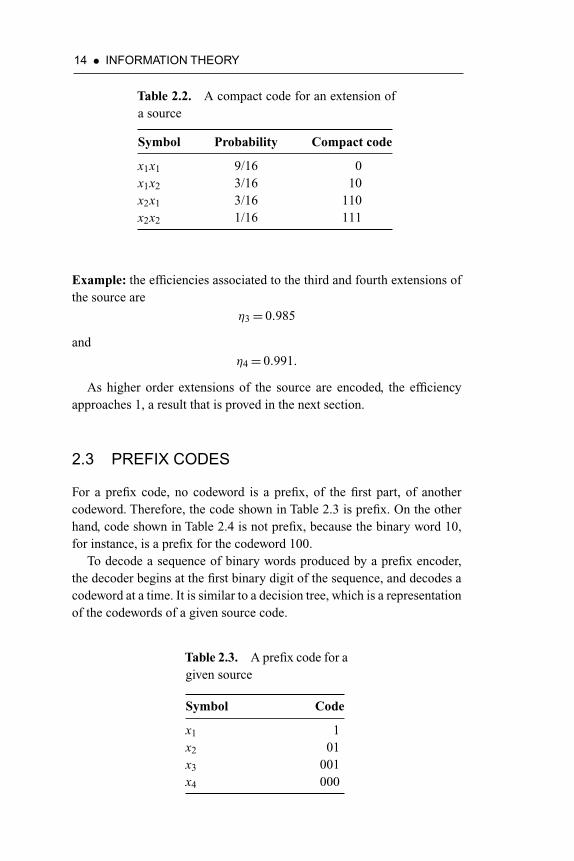
Table 2.2. A compact code for an extension ofa source
Symbol Probability Compact code
x1x1 9/16 0x1x2 3/16 10x2x1 3/16 110x2x2 1/16 111
Example: the efficiencies associated to the third and fourth extensions ofthe source are
η3= 0.985
andη4= 0.991.
As higher order extensions of the source are encoded, the efficiencyapproaches 1, a result that is proved in the next section.
2.3 PREFIX CODES
For a prefix code, no codeword is a prefix, of the first part, of anothercodeword. Therefore, the code shown in Table 2.3 is prefix. On the otherhand, code shown in Table 2.4 is not prefix, because the binary word 10,for instance, is a prefix for the codeword 100.
To decode a sequence of binary words produced by a prefix encoder,the decoder begins at the first binary digit of the sequence, and decodes acodeword at a time. It is similar to a decision tree, which is a representationof the codewords of a given source code.
Table 2.3. A prefix code for agiven source
Symbol Code
x1 1x2 01x3 001x4 000

SOURCES OF INFORMATION • 15
Table 2.4. A source code thatis not prefix
Symbol Code
x1 1x2 10x3 100x4 1000
Figure 2.2 illustrates the decision tree for the prefix code pointed inTable 2.5.
The tree has one initial state and four final states, which correspond tothe symbols x1, x2, and x3. From the initial state, for each received bit, thedecoder searches the tree until a final state is found.
The decoder, then, emits a corresponding decoded symbol and returnsto the initial state. Therefore, from the initial state, after receiving a 1,the source decoder decodes symbol x1 and returns to the initial state. If itreceives a 0, the decoder moves to the lower part of the tree, in the following,after receiving another 0, the decoder moves further to the lower part ofthe tree and, after receiving a 1, the decoder retrieves x2 and returns to theinitial state.
Considering the code from Table 2.5, with the decoding tree fromFigure 2.2, the binary sequence 011100010010100101 is decoded into theoutput sequence x1x0x0x3x0x2x1x2x1.
By construction, a prefix code is always unequivocally decodable, whichis important to avoid any confusion at the receiver.
Consider a code that has been constructed for a discrete source withalphabet {x1, x2, . . . , xK }. Let {p1, p1, . . . , pK } be the source statistics,and lk be the codeword length for symbol xk , k = 1, . . . , K . If the binarycode constructed for the source is a prefix one, then one can use the
Table 2.5. Example of a prefix code
Source symbol Probability of occurrence Code
x0 0.5 1x1 0.25 01x2 0.125 001x3 0.125 000

16 • INFORMATION THEORY
x0
x1
x2
x3
0
0
0
1
1
1
Initialstate
Figure 2.2. Decision tree for the code in Table 2.5.
Kraft-McMillan inequality
K∑k=1
2−lk ≤ 1, (2.6)
in which factor 2 is the radix, or number of symbols, of the binary alphabet.For a memoryless discrete source with entropy H (X ), the codeword
average length of a prefix code is limited to
H (X )≤L < H (X )+ 1. (2.7)
The left hand side equality is obtained on the condition that symbol xk beemitted from the source with probability pk = 2−lk , in which lk is the lengthof the codeword assigned to symbol xk .
Consider the N th order extension of a memoryless discrete source. Forthe N th order extension of a code, the encoder operates on blocks of Nsymbols from the original source, instead of individual ones, and the sourcealphabet X N has an entropy that is N times the entropy of the originalsource.
Let LN be the average length for the extended prefix code. For anunequivocally decodable code, LN is as small as possible, from Equa-tion 2.7 it follows that
H (X N )≤LN < H (X N )+ 1, (2.8)
therefore,
NH (X )≤LN < NH (X )+ 1, (2.9)

SOURCES OF INFORMATION • 17
or, in an equivalent way,
H (X )≤ LN
N< H (X )+ 1
N. (2.10)
In the limit, as N goes to infinity, the inferior and superior limitantsconverge, and therefore,
limN→∞
1
NLN =H (X ). (2.11)
Therefore, for a prefix extended encoder, as the order N increases, thecode represents the source as efficiently as desired, and the average code-word length can be as close to the source entropy as possible, according toShannon’s source coding theorem. On the other hand, there is a compromisebetween the reduction on the average codeword length and the increase incomplexity of the decoding process (Haykin 1988).
2.4 THE INFORMATION UNIT
There is some confusion between the binary digit, abbreviated as bit, andthe information particle, also baptized as bit by John Tukey and ClaudeShannon.
In a meeting of the Institute of Electrical and Electronics Engineers(IEEE) the largest scientific institution in the World, the author of this bookproposed the shannon [Sh] as a unit of information transmission, equivalentto bit per second. It is instructive to say that the bit, as used today, is not aunit of information, because it is not approved by the International Systemof Units (SI).
What is curious about that meeting was the misunderstanding thatsurrounded the units, in particular regarding the difference between theconcepts of information unit and digital logic unit.
To make things clear, the binary digit is associated to a certain state of adigital system, and not to information. A binary digit 1 can refer to 5 volts,in TTL logic, or 12 volts, for CMOS logic.
The information bit exists independent of any association to a particularvoltage level. It can be associated, for example, to a discrete informationor to the quantization of an analog information.
For instance, the information bits recorded on the surface of a com-pact disk are stored as a series of depressions on the plastic material,which are read by an optical beam, generated by a semiconductor laser.But, obviously, the depressions are not the information. They represent a

18 • INFORMATION THEORY
means for the transmission of information, a material substrate that carriesthe data.
In the same way, the information can exist, even if it is not associatedto light or other electromagnetic radiation. It can be transported by severalmeans, including paper, and materializes itself when it is processed by acomputer or by a human being.
CHAPTER 3
SOURCE CODING
3.1 TYPES OF SOURCE CODES
This chapter presents the classification of source codes, block codes, non-singular codes, uniquely decodable codes, and instantaneous codes.
3.1.1 BLOCK CODES
Let S ={x0, x1, . . . , xK−1} be a set of symbols of a given source alphabet.A code is defined as a mapping of all possible symbol sequences from S intosequences of another set X ={x0, x1, . . . , xM−1}, called the code alphabet.
A block code maps each of the symbols from the source set into asequence of the code alphabet. The fixed sequences of symbols xj arecalled codewords Xi. Note that Xi denotes a sequence of xj’s (Abramson1963).
Example: a binary block code is presented in Table 3.1, and a ternary blockcode is shown in Table 3.2.
3.1.2 NONSINGULAR CODES
A block code is said to be nonsingular if all codewords are distinct(Abramson 1963). Table 3.2 shows an example of a nonsingular code.The code shown in Table 3.3 is also nonsingular, but although the code-words are distinct there is a certain ambiguity between some symbolsequences of the code regarding the source symbol sequences.

20 • INFORMATION THEORY
Table 3.1. A binary block code
Source symbols Code
x0 0x1 11x2 00x3 1
Table 3.2. A ternary block code
Source symbols Code
x0 0x1 1x2 2x3 01
Table 3.3. A nonsingular block code
Source symbols Code
x0 0x1 01x2 1x3 11
Example: the sequence 1111 can correspond to x2x2x2x2, or x2x3x2, oreven x3x3. Which indicates that it is necessary to define a more strict con-dition than nonsingularity for a code, to guarantee that it can be used in apractical situation.
3.1.3 UNIQUELY DECODABLE CODES
Let a block code map symbols from a source alphabet S into fixed symbolsequences of a code alphabet X . The source can be an extension of anothersource, which is composed of symbols from the original alphabet. Then-ary extension of a block code that maps symbols xi into codewords Xi isthe block code that maps symbol sequences from the source (xi1xi2 . . . xin)into the codeword sequences (Xi1Xi2 . . . Xin) (Abramson 1963).

SOURCE CODING • 21
Table 3.4. A nonsingular block code
Source symbols Code
x0 1x1 00x2 11x3 10
Table 3.5. The second extension of a block code
Source symbols Code Source symbols Code
x0x0 11 x2x0 111x0x1 100 x2x1 1100x0x2 111 x2x2 1111x0x3 110 x2x3 1110x1x0 001 x3x0 101x1x1 0000 x3x1 1000x1x2 0011 x3x2 1011x1x3 0010 x3x3 1010
From the previous definition, the n-ary extension of a block code is alsoa block code. The second order extension of the block code presented inTable 3.4 is the block code of Table 3.5.
A block code is said to be uniquely decodable if and only if the n-aryextension of the code is nonsingular for all finite n.
3.1.4 INSTANTANEOUS CODES
Table 3.6 presents two examples of uniquely decodable codes. Code Ais a simpler method to construct a uniquely decodable set of sequences,because all codewords have the same length and it is a nonsingularcode.
Code B is also uniquely decodable. It is also called a commacode, because the digit zero is used to separate the codewords (Abram-son 1963).
Consider the code shown in Table 3.7. Code C differs from A and Bfrom Table 3.6 in an important aspect. If a binary sequence composed ofcodewords from code C occurs, it is not possible to decode the sequence.

22 • INFORMATION THEORY
Table 3.6. Uniquely decodable codes
Source symbols Code A Code Bx0 000 0x1 001 10x2 010 110x3 011 1110x4 100 11110x5 101 111110x6 110 1111110x7 111 11111110
Table 3.7. Another uniquely decodable code
Source symbols Code Cx0 1x1 10x2 100x3 1000x4 10000x5 100000x6 1000000x7 10000000
Example: if the bit stream 100000 is received, for example, it is not pos-sible to decide if it corresponds to symbol x5, unless the next symbol isavailable. If the next symbol is 1, then the sequence is 100000, but if it is 0,then it is necessary to inspect one more symbol to know if the sequencecorresponds to x6 (1000000) or x7 (10000000).
A uniquely decodable code is instantaneous if it is possible to decodeeach codeword in a sequence with no reference to subsequent symbols(Abramson 1963). Code A and B are instantaneous, and C is not.
It is possible to devise a test to indicate when a code is instantaneous.Let Xi= xi1xi2 . . . xim be a word from a certain code. The sequence of sym-bols (xi1xi2 . . . xij), with j≤m, is called the prefix of the codeword Xi.
Example: the codeword 10000 has five prefixes: 1, 10, 100, 1000, and10000. A necessary condition for a code to be instantaneous is that nocodeword is a prefix of another codeword.

SOURCE CODING • 23
Codes
Block Nonblock
Nonsingular Singular
Uniquelydecodable
Nonuniquelydecodable
Instantaneous Noninstantaneous
Figure 3.1. Classes of source codes.
The various classes of codes presented in this section are summarizedin Figure 3.1.
3.2 CONSTRUCTION OF INSTANTANEOUSCODES
In order to construct a binary instantaneous code for a source with fivesymbols, one can begin by attributing the digit 0 to symbol s0 (Abramson1963)
x0← 0.
In this case, the remaining source symbols should correspond to thecodewords that begin with the digit 1. Otherwise, it is not a prefix code. Itis not possible to associate x1 to the codeword 1, because no other symbolwould remain to begin the other codewords.
Therefore,x1← 10.
This codeword assignment requires that the remaining codewords beginwith 11. If
x2← 110
then, the only unused prefix with three bits is 111, which implies that
x3← 1110
and
x4← 1111.

24 • INFORMATION THEORY
In the previously constructed code, note that if one begins the codeconstruction by making x0 to correspond to 0, this restricts the availablenumber of codewords, because the remaining codewords had to, necessar-ily, begin with 1.
On the other hand, if a two-digit word had been chosen to represent x0,there would be more freedom to choose the others, and there would be noneed to assign very long codewords to the last ones.
A binary instantaneous code can be constructed to represent the fivesymbols (Abramson 1963). The first assignment is
x0← 00.
Then, one can assign
x1← 01
and two unused prefixes of length two are saved to the following codewordassignment:
x2← 10
x3← 110
x4← 111.
The question of which code is the best is postponed for the next section,because it requires the notion of average length of a code, that depends onthe symbol probability distribution.
3.3 KRAFT INEQUALITY
Consider an instantaneous code with source alphabet given by
S ={x0, x1, . . . , xK−1}and code alphabet
X ={x0, x1, . . . , xM−1}.Let X0, X1, . . . , XK−1 be the codewords, and let li be the length of the
word Xi. The Kraft inequality establishes that a necessary and sufficientcondition for the existence of an instantaneous code of length l0, l1, . . . ,lK−1 is
K−1∑i=0
r−li ≤ 1, (3.1)
in which r is the number of different symbols of the code.

SOURCE CODING • 25
For the binary case,
K−1∑i=0
2−li ≤ 1. (3.2)
The Kraft inequality can be used to determine if a given sequence oflength li is acceptable for a codeword of an instantaneous code.
Consider an information source, with four possible symbols, x0, x1,x2, and x3. Table 3.8 presents five possible codes to represent the originalsymbols, using a binary alphabet.
Example: for code A, one obtains
3∑i=0
2−li = 2−2 + 2−2 + 2−2 + 2−2= 1.
Therefore, the codeword lengths of this code are acceptable for an instan-taneous code. But, the Kraft inequality does not tell if A is an instanta-neous code. It is only a necessary condition that has to be fulfilled by thelengths.
For the example, the inequality states that there is an instantaneouscode with four codewords of length 2. In this case, it is clear that thebinary codewords of code A satisfy the Kraft inequality and also form aninstantaneous code.
For code B,
3∑i=0
2−li = 2−1 + 2−3 + 2−3 + 2−3= 7/8≤ 1.
In this case, the lengths of the codewords are suitable to compose aninstantaneous code. Code B is also a prefix code.
Table 3.8. Selected binary codes
Source symbols Code A Code B Code C Code D Code Ex0 11 1 1 1 1x1 10 011 01 011 01x2 01 001 001 001 001x3 00 000 000 00 00
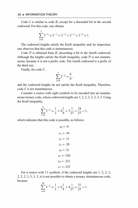
26 • INFORMATION THEORY
Code C is similar to code B, except for a discarded bit in the secondcodeword. For this code, one obtains
3∑i=0
2−li = 2−1 + 2−2 + 2−3 + 2−3= 1.
The codeword lengths satisfy the Kraft inequality and, by inspection,one observes that this code is instantaneous.
Code D is obtained from B, discarding a bit in the fourth codeword.Although the lengths satisfy the Kraft inequality, code D is not instanta-neous, because it is not a prefix code. The fourth codeword is a prefix ofthe third one.
Finally, for code E ,3∑
i=0
2−li = 9
8,
and the codeword lengths do not satisfy the Kraft inequality. Therefore,code E is not instantaneous.
Consider a source with eight symbols to be encoded into an instanta-neous ternary code, whose codeword lengths are 1, 2, 2, 2, 2, 3, 3, 3. Usingthe Kraft inequality,
9∑i=0
3−li = 1
3+ 4
1
9+ 3
1
27= 24
27< 1,
which indicates that this code is possible, as follows:
x0← 0
x1← 10
x2← 11
x3← 20
x4← 21
x5← 220
x6← 221
x7← 222
For a source with 11 symbols, if the codeword lengths are 1, 2, 2, 2,2, 2, 2, 3, 3, 3, 3, it is not possible to obtain a ternary instantaneous code,because
10∑i=0
3−li = 1
3+ 6
1
9+ 4
1
27= 31
27> 1.

SOURCE CODING • 27
3.4 HUFFMAN CODE
This section describes the Huffman coding algorithm, and the procedureto construct the Huffman code when the source statistics are known.
The technique was developed by David Albert Huffman (1925–1999),in a paper for a course on Information Theory taught by Robert Mario Fano(1917–), at the Massachusetts Institute of Technology (MIT). The obtainedsequences are called Huffman codes, and they are prefix codes.
Huffman procedure is based on two assumptions regarding the optimumprefix codes:
1. The most frequent symbols, those with higher probability, are rep-resented by shorter codewords.
2. The least frequent symbols are assigned codewords of same length.
According to the first assumption, as the most probable symbols arealso the most frequent, they must be as short as possible to decrease theaverage length of the code. The second assumption is also true, becausefor a prefix code a shorter codeword could not be a prefix of another one.The least probable symbols must be distinct and have same length (Sayood2006).
Furthermore, the Huffman process is completed by the addition of asimple requisite. The longer codewords that correspond to the least fre-quent symbols differ only on the last digit.
3.4.1 CONSTRUCTING A BINARY HUFFMAN CODE
Given a discrete source, a Huffman code can be constructed along thefollowing steps:
1. The source symbols are arranged in decreasing probability. Theleast probable symbols receive the assignments 0 and 1.
2. Both symbols are combined to create a new source symbol, whoseprobability is the sum of the original ones. The list is reduced byone symbol. The new symbol is positioned in the list according toits probability.
3. This procedure continues until the list has only two symbols, whichreceive the assignments 0 and 1.
4. Finally, the binary codeword for each symbol is obtained by areverse process.

28 • INFORMATION THEORY
Table 3.9. Discrete source with fivesymbols and their probabilities
Symbols Probabilities
x0 0.4x1 0.2x2 0.2x3 0.1x4 0.1
In order to explain the algorithm, consider the source of Table 3.9.The first phase is to arrange the symbols in a decreasing order of prob-
ability. Assign the values 0 and 1 to the symbols with the smallest proba-bilities. They are then combined to create a new symbol. The probabilityassociated to the new symbol is the sum of the previous probabilities. Thenew symbol is repositioned in the list, to maintain the same decreasingorder for the probabilities. The procedure is shown in Figure 3.2.
The procedure is repeated until only two symbols remain, which areassigned to 0 and 1, as shown in Figure 3.3.
The procedure is repeated to obtain all codewords, by reading the digitsin inverse order, from Phase IV to Phase I, as illustrated in Figure 3.4.Following the arrows, for symbol x4 one finds the codeword 011.
0.1
0.40.2
0.20.2
0.20.1
0.40.2
01
Symbol Phase Ix0x1
x3x4
x2
Figure 3.2. Probabilities in descending order for the Huffman code.
0.4
0.1
0.40.2
0.20.2
0.20.1
0.40.2 0.4
0.2
0.4 0.6
01
01
10
01
Symbol Phase I Phase II Phase III Phase IVx0x1x2x3x4
Figure 3.3. Huffman code.At each phase, the two least probable symbolsare combined.

SOURCE CODING • 29
0.4
0.1
0.40.2
0.20.2
0.20.1
0.40.2 0.4
0.2
0.4 0.6
01
01
10
01
Symbol Phase I Phase II Phase III Phase IVx0x1x2x3x4
(a)
x0x1x2x3x4 0110.1
0.40.20.20.1
001011010
Symbol CodewordProbability
(b)
Figure 3.4. (a) Example of the Huffman coding algorithm to obtain thecodewords. (b) Resulting code.
For the example, the average codeword length for the Huffman code isgiven by
L=4∑
i=0
pk lk = 0, 4(2)+ 0, 2(2)+ 0, 2(2)+ 0, 1(3)+ 0, 1(3)= 2.2 bits.
The source entropy is calculated as
H (X )=4∑
i=0
pk log2
(1
pk
)
H (X )= 0, 4 log2
(1
0, 4
)+ 0, 2 log2
(1
0, 2
)+ 0, 2 log2
(1
0, 2
)
+ 0, 1 log2
(1
0, 1
)+ 0, 1 log2
(1
0, 1
),
or,
H (X )= 2.12193 bits.
The code efficiency is
η= H (X )
L= 2.12193
2.2,
which is equal to 96.45 percent.It is important to say that the Huffman procedure is not unique, and
several variations can be obtained for the final set of codewords, depending

30 • INFORMATION THEORY
Table 3.10. Four distinct Huffman codes obtained for thesource of Table 3.9
Symbols Code I Code II Code III Code IV
x0 00 11 1 0x1 10 01 01 10x2 11 00 000 111x3 010 101 0010 1101x4 011 100 0011 1100
on the way the bits are assigned. But, in spite of how the probabilities arepositioned, the average length is always the same, if the rules are followed.
The difference is the variance of the codeword lengths, defined as
V[L]=K−1∑k=0
pk (lk − L)2, (3.3)
in which pk and lk denote the probability of occurrence of the k-th sourcesymbol, and length of the respective codeword.
Usually, the procedure of displacing the probability of the new symbolto the highest position in the list produces smaller values for V[L], ascompared to the displacement of the probability to the lowest position ofthe list.
Table 3.10 presents four Huffman codes obtained for the source ofTable 3.9. Codes I and II were obtained shifting the new symbol to thehighest position in the list of decreasing probabilities.
Codes III and IV were produced by shifting the new symbol to thelowest position in the list. Codes I and III used the systematic assignmentof 0 followed by 1 to the least frequent symbols. Codes II and IV used thesystematic assignment of 1 followed by 0 to the least frequent symbols.For all codes the average codeword length is 2.2 bits. For codes I and II,the variance of the codeword lengths is 0.16. For codes III and IV, thevariance is 1.36.
CHAPTER 4
INFORMATION TRANSMISSION
Claude Elwood Shannon (1916–2001) is considered the father of Informa-tion Theory. In 1948, he published a seminal article on the mathematicalconcept of information, which is one of the most cited for decades. Infor-mation left the Journalism field to occupy a more formal area, as part ofProbability Theory.
The entropy, in the context of information theory, was initially definedby Ralph Vinton Lyon Hartley (1888–1970), in the article “Transmissionof Information”, published by Bell System Technical Journal in July 1928,10 years before the formalization of the concept by Claude Shannon.
Shannon’s development was also based on Harry Nyquist’s work (HarryTheodor Nyqvist, 1889–1976), which determined the sampling rate, as afunction of frequency, necessary to reconstruct an analog signal using a setof discrete samples.
In an independent way, Andrei N. Kolmogorov developed his Complex-ity Theory, during the 1960’s. It was a new information theory, based onthe length of an algorithm developed to describe a certain data sequence.He used Alan Turing’s machine in this new definition. Under certain con-ditions, Kolmogorov’s and Shannon’s definitions are equivalent.
The idea of relating the number of states of a system with a physical mea-sure, although, dates back to the 19th century. Rudolph Clausius proposedthe term entropy for such a measure in 1895.
Entropy comes from the Greek word for transformation and in Physics,it is related to the logarithm of the ratio between the final and initial temper-ature of a system, or to the ratio of the heat variation and the temperatureof the same system.
Shannon defined the entropy of an alphabet at the negative of the meanvalue of the logarithm of the symbols’ probability. This way, when thesymbols are equiprobable, the definition is equivalent to that of Nyquist’s.

32 • INFORMATION THEORY
But, as a more generic definition, Shannon’s entropy can be usedto compute the capacity of communication channels. Most part of theresearchers’ work is devoted to either compute the capacity or to developerror-correcting codes to attain that capacity.
Shannon died on February 24, 2001, as a victim of a disease named afterthe physician Aloysius Alzheimer. According to his wife, he lived a quietlife, but had lost his capacity to retain information.
4.1 THE CONCEPT OF INFORMATION THEORY
The concept of information transmission is associated with the existenceof a communication channel that links the source and destination of themessage. This can imply the occurrence of transmission errors, caused bythe probabilistic nature of the channel. Figure 4.1 illustrates the canonicalmodel for a communication channel, proposed by Shannon in his seminalpaper of 1948. This is a very simplified model of reality, but contains thebasic blocks upon which the mathematical structure is built.
4.2 JOINT INFORMATION MEASUREMENT
Consider two discrete and finite sample spaces, � and �, with the associ-ated random variables X and Y ,
X = x1, x2, . . . , xN ,
Y = y1, y2, . . . , yM . (4.1)
The events from � may jointly occur with events from �. Therefore,the following matrix contains the whole set of events in the product
Transmitter Receiver
Noise
Channel
Figure 4.1. Model for a communication channel.
INFORMATION TRANSMISSION • 33
space ��,
[XY ]=
⎡⎢⎢⎣
x1y1 x1y2 · · · x1yM
x2y1 x2y2 · · · x2yM
· · · · · · · · · · · ·xN y1 xN y2 · · · xN yM
⎤⎥⎥⎦ (4.2)
The joint probability matrix is given in the following in which no restric-tion is assumed regarding the dependence between the random variables.
[P(X , Y )]=
⎡⎢⎢⎣
p1,1 p1,2 · · · p1,M
p2,1 p2,2 · · · p2,M
· · · · · · · · · · · ·pN ,1 pN ,2 · · · pN ,M
⎤⎥⎥⎦ (4.3)
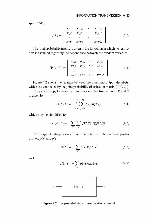
Figure 4.2 shows the relation between the input and output alphabets,which are connected by the joint probability distribution matrix [P(X , Y )].
The joint entropy between the random variables from sources X and Yis given by
H (X , Y )=−N∑
k=1
M∑j=1
pk ,j log pk ,j , (4.4)
which may be simplified to
H (X , Y )=−∑
X
∑Y
p(x, y) log p(x, y). (4.5)
The marginal entropies may be written in terms of the marginal proba-bilities, p(x) and p(y)
H (X )=−∑
X
p(x) log p(x) (4.6)
and
H (Y )=−∑
Y
p(y) log p(y). (4.7)
[ P(X,Y) ] X Y
Figure 4.2. A probabilistic communication channel.
34 • INFORMATION THEORY
4.3 CONDITIONAL ENTROPY
The concept of conditional entropy is essential to model, and understand, theoperation of the communication channel, because it provides informationabout a particular symbol, given that another symbol has occurred. Theentropy of alphabet X conditioned to the occurrence of a particular symboly is given by
H (X |y)= −∑
X
p(x, y)
p(y)log
p(x, y)
p(y)
= −∑
X
p(x|y) log p(x|y). (4.8)
The expected value of the conditional entropy, for all possibles valuesof y, provides the average conditional entropy of the system,
H (X |Y )=E[H (X |y)]=∑
Y
p(y)[H (X |y)]
= −∑
Y
p(y)∑
X
p(x|y) log p(x|y), (4.9)
which can be written as
H (X |Y )=−∑
Y
∑X
p(y)p(x|y) log p(x|y), (4.10)
or
H (X |Y )=−∑
Y
∑X
p(x, y) log p(x|y). (4.11)
In the same way, the mean conditional entropy of source Y , given theinformation about source X , is
H (Y |X )=−∑
X
∑Y
p(x)p(y|x) log p(y|x), (4.12)
or
H (Y |X )=−∑
X
∑Y
p(x, y) log p(y|x). (4.13)
4.4 MODEL FOR A COMMUNICATION CHANNEL
A communication channel can be modeled based on the previous devel-opments. Consider a source that has the given alphabet X . The source

INFORMATION TRANSMISSION • 35
transmits the information to the destiny using a certain channel. The sys-tem maybe described by a joint probability matrix, which gives the jointprobability of occurrence of a transmitted symbol and a received one,
[P(X , Y )]=
⎡⎢⎢⎣
p(x1, y1) p(x1, y2) · · · p(x1, yN )p(x2, y1) p(x2, y2) · · · p(x2, yN )· · · · · · · · · · · ·
p(xM , y1) p(xM , y2) · · · p(xM , yN )
⎤⎥⎥⎦ (4.14)
There are five probability schemes to analyze:
1. [P(X , Y )], joint probability matrix,2. [P(X )], marginal probability matrix of X ,3. [P(Y )], marginal probability matrix of Y ,4. [P(X |Y )], probability matrix conditioned on Y ,5. [P(Y |X )], probability matrix conditioned on X .
Those probability schemes produce five entropy functions, associatedto the communication channel, whose interpretations are given as follows:
1. H (X )—Average information per source symbol, or source entropy,2. H (Y )—Average information per received symbol, or receiver
entropy,3. H (X , Y )—Average information associated to pairs of transmitted
and received symbols, or average uncertainty of the communicationsystem,
4. H (X |Y )—Average information measurement of the receivedsymbol, given that X was transmitted, or conditional entropy,
5. H (Y |X )—Average information measurement of the source, giventhat Y was received, or equivocation.
4.5 NOISELESS CHANNEL
For the noiseless discrete channel, each symbol from the input alphabet hasa one-to-one correspondence with the output. The joint probability matrix,as well as, the transition probability matrix, has the same diagonal format,
[P(X , Y )]=
⎡⎢⎢⎣
p(x1, y1) 0 · · · 00 p(x2, y2) · · · 0· · · · · · · · · · · ·0 0 · · · p(xN , yN )
⎤⎥⎥⎦ (4.15)

36 • INFORMATION THEORY
[P(X |Y )]= [P(Y |X )]=
⎡⎢⎢⎣
1 0 · · · 00 1 · · · 0· · · · · · · · · · · ·0 0 · · · 1
⎤⎥⎥⎦ (4.16)
The joint entropy equals the marginal entropies
H (X , Y )=H (X )=H (Y )=−N∑
i=1
p(xi, yi) log p(xi, yi), (4.17)
and the conditional entropies are null
H (Y |X )=H (X |Y )= 0. (4.18)
As a consequence, the receiver uncertainty is equal to the sourceentropy, and there is no ambiguity at the reception, which indicates thatthe conditional entropies are all zero.
4.6 CHANNEL WITH INDEPENDENT OUTPUTAND INPUT
For the channel with independent input and output, there is no relationbetween the transmitted and received symbols, that is, given that a givensymbol has been transmitted, any symbol can be received, with no con-nection whatsoever with it. The joint probability matrix has N identicalcolumns
[P(X , Y )]=
⎡⎢⎢⎣
p p1 · · · p1
p2 p2 · · · p2
· · · · · · · · · · · ·pM pM · · · pM
⎤⎥⎥⎦ ,
M∑i
pi= 1
N. (4.19)
The input and output symbol probabilities are statistically independent,that is,
p(x, y)= p(x)p(y). (4.20)
Computing the entropy gives
H (X , Y )=−N
(M∑
i=1
pi log pi
), (4.21)
H (X )=−M∑
i=1
Npi log Npi=−N
(M∑
i=1
pi log pi
)− log N , (4.22)

INFORMATION TRANSMISSION • 37
H (Y )= − N
(1
Nlog
1
N
)= log N , (4.23)
H (X |Y )= −M∑
i=1
Npi log Npi=H (X ), (4.24)
H (Y |X )= −M∑
i=1
Npi log1
N= log N =H (Y ). (4.25)
As a consequence, the channel with independent input and output doesnot provide information, that is, has the highest possible loss, contrastingwith the noiseless channel.
4.7 RELATIONS BETWEEN THE ENTROPIES
It is possible to show, using Bayes rule for the conditional probability, thatthe joint entropy can be written in terms of the conditional entropy, in thefollowing way
H (X , Y )=H (X |Y )+ H (Y ), (4.26)
H (X , Y )=H (Y |X )+ H (X ). (4.27)
Shannon has shown the fundamental inequality
H (X )≥H (X |Y ), (4.28)
whose demonstration is given in the following.The logarithm concavity property can be used to demonstrate the inequal-
ity, lnx≤ x − 1, as follows,
H (X |Y )− H (X )=∑
Y
∑X
p(x, y) logp(x)
p(x|y)
≤∑
Y
∑X
p(x, y)(
p(x)
p(x|y)− 1)
log e. (4.29)
But, the right hand side of the inequality is zero, as shown in thefollowing
∑Y
∑X
(p(x) · p(y)− p(x, y)) log e=∑
Y
(p(y)− p(y)) log e
= 0. (4.30)

38 • INFORMATION THEORY
Therefore,
H (X )≥H (X |Y ). (4.31)
In a similar manner, it can be shown that
H (Y )≥H (Y |X ). (4.32)
The equality is attained if and only if X and Y are statistically independent.
4.8 MUTUAL INFORMATION
A measure of mutual information provided by two symbols (xi, yi) can bewritten as
I (xi; yj)= log2 p(xi|yj)− log2 p(xi)
= log2p(xi|yj)
p(xi)= log
p(xi, yj)
p(xi)p(yj). (4.33)
It can be noticed that the a priori information of symbol xi is containedin the marginal probability p(xi). The a posteriori probability that sym-bol xi has been transmitted, given that yi was received is p(xi|yi). There-fore, in an informal way, the information gain for the observed symbolequals the difference between the initial information, or uncertainty, andthe final one.
The mutual information is continuous in p(xi|yi), and also symmet-ric, or
I (xi; yj)= I (yj; xi), (4.34)
which indicates that the information provided by xi about yi is the sameprovided by yi about xi.
The function I (xi; xi) can be called the auto-information of xi, or
I (xi)= I (xi; xi)= log1
p(xi), (4.35)
because, for an observer of the source alphabet, the a priori knowledge ofthe situation is that xi will be transmitted with probability p(xi), and the aposteriori knowledge is the certainty that xi transmitted.
In conclusion,
I (xi; yj)≤ I (xi; xi)= I (xi), (4.36)
I (xi; yj)≤ I (yj; yj)= I (yj). (4.37)

INFORMATION TRANSMISSION • 39
The statistical mean of the mutual information per pairs of symbolsprovides an interesting interpretation of the mutual information concept,
I (X ; Y )=E[I (xi; yj)]=∑
i
∑j
p(xi, yj)I (xi; yj), (4.38)
which can be written as
I (X ; Y )=∑
i
∑j
p(xi, yj) logp(xi|yj)
p(xi). (4.39)
The average mutual information can be interpreted as a reduction onthe uncertainty about the input X , when the output Y is observed (MacKay2003). This definition provides an adequate metric for the average mutualinformation of all pairs of symbols, and can be put in terms of the entropy,such as
I (X ; Y )=H (X )+ H (Y )− H (X , Y ), (4.40)
I (X ; Y )=H (X )− H (X |Y ), (4.41)
I (X ; Y )=H (Y )− H (Y |X ). (4.42)
Put that way, the average mutual information gives a measure of theinformation that is transmitted by the channel. Because of this, it is calledtransinformation, or information transferred by the channel. It is alwaysnon-negative, even if the individual information quantities are negative forcertain pairs of symbols.
For a noiseless channel, the average mutual information equals the jointentropy.
I (X ; Y )=H (X )=H (Y ), (4.43)
I (X ; Y )=H (X , Y ). (4.44)
On the other hand, for a channel in which the output is independent of theinput, the average mutual information is null, implying that no informationis transmitted by the channel.
I (X ; Y )=H (X )− H (X |Y ),
=H (X )− H (X )= 0. (4.45)
It is possible to use the set theory, presented in the Appendix, to obtaina pictorial interpretation of the fundamental inequalities discovered byShannon. Consider, the set of events A and B, associated to the set ofsymbols X and Y , and a Lebesgue measure m. It is possible to associate,

40 • INFORMATION THEORY
unambiguously, the measures of A and B with the entropies of X and Y(Reza 1961),
m(A)←→H (X ), (4.46)
m(B)←→H (Y ). (4.47)
In the same way, one can associate the joint and conditional entropiesthe union and intersection of sets, respectively,
m(A ∪ B)←→H (X , Y ), (4.48)
m(AB)←→H (X |Y ), (4.49)
m(BA)←→H (Y |X ). (4.50)
The average mutual information is, therefore, associated to the measureof the intersection of the sets,
m(A ∩ B)←→ I (X ; Y ). (4.51)
Those relations can be seen in Figure 4.3, which also serve as a meansto memorize the entropy and mutual information properties.
Therefore, the fundamental inequalities can be written as a result of setoperations (Reza 1961),
m(A ∪ B)≤m(A)+ m(B)←→H (X , Y )≤H (X )+ H (Y ), (4.52)
m(AB) ≤ m(A)←→H (X |Y )≤H (X ), (4.53)
m(BA) ≤ m(B)←→H (Y |X )≤H (Y ), (4.54)
and, finally,
m(A ∪ B)=m(AB)+ m(BA)+ m(A ∩ B), (4.55)
which is equivalent to
H (X , Y )=H (X |Y )+ H (Y |X )+ I (X ; Y ). (4.56)
BA A∩B
Ω
Figure 4.3. Venn diagram corresponding to the relation between theentropies.
INFORMATION TRANSMISSION • 41
For a noiseless channel, the two sets coincide, and the relations can bewritten as:
m(A)=m(B)←→H (X )=H (Y ), (4.57)
m(A ∪ B)=m(A)=m(B)←→H (X , Y )=H (X )=H (Y ), (4.58)
m(AB)= 0←→H (X |Y )= 0, (4.59)
m(BA)= 0←→H (Y |X )= 0, (4.60)
and, finally,
m(A ∩ B)=m(A)=m(B)=m(A ∪ B)
←→ I (X ; Y )=H (X )=H (Y )=H (X , Y ). (4.61)
For a channel with output symbols independent from the input symbols,the sets A and B are considered mutually exclusive, therefore:
m(A ∪ B)=m(A)+ m(B)←→H (X , Y )=H (X )+ H (Y ) (4.62)
m(AB)=m(A)←→H (X |Y )=H (X ) (4.63)
m(A ∩ B)= 0←→ I (X ; Y )= 0. (4.64)
The same procedure can be applied to a multiple port channel. For athree port channel, one can obtain the following relations for the entropies:
H (X , Y , Z)≤H (X )+ H (Y )+ H (Z), (4.65)
H (Z |X , Y )≤H (Z |Y ). (4.66)
In the same reasoning, it is possible to obtain the following relations forthe average mutual information for a three-port channel:
I (X ; Y , Z)= I (X ; Y )+ I (X ; Z |Y ), (4.67)
I (Y , Z ; X )= I (Y ; X )+ I (Z ; X |Y ). (4.68)
4.9 CHANNEL CAPACITY
Shannon defined the discrete channel capacity as the maximum of theaverage mutual information, computed for all possible probability sets that

42 • INFORMATION THEORY
can be associated to the input symbol alphabet, that is, for all memorylesssources,
C=max I (X ; Y )=max [H (X )− H (X |Y )]. (4.69)
4.9.1 CAPACITY OF THE MEMORYLESS DISCRETECHANNEL
Consider X as the alphabet of a source with N symbols. Because the tran-sition probability matrix is diagonal, one obtains
C=max I (X ; Y )=max [H (X )]=max
[−
N∑i=1
p(xi) log p(xi)
]. (4.70)
Example: the entropy attains a maximum when all symbols are equiprob-able. Therefore, for the memoryless discrete channel, the capacity is
C=max
[−
N∑i=1
1
Nlog
1
N
],
which gives
C= log N bits per symbol. (4.71)
The channel capacity can also be expressed in bits per second, or shannon(Sh), and corresponds to the information transmission rate of the channel,for symbols with duration T seconds,
CT = C
Tbits per second, or Sh. (4.72)
Therefore, for the noiseless channel,
CT = C
T= 1
Tlog N bits per second, or Sh. (4.73)
4.9.2 RELATIVE REDUNDANCY AND EFFICIENCY
The absolute redundancy is the difference between the actual informationtransmission rate and I (X ; Y ) and the maximum possible value,

INFORMATION TRANSMISSION • 43
Absolute redundancy for a noisy channel=C − I (X ; Y )
= log N − H (X ). (4.74)
The ratio between the absolute redundancy and the channel capacity isdefined as the system relative redundancy,
Relative redundancy for a noiseless channel, D= log N − H (X )
log N
= 1− H (X )
log N. (4.75)
The system efficiency is defined as the complement of the relativeredundancy,
Efficiency of the noiseless channel, E= I (X ; Y )
log N= H (X )
log N= 1− D. (4.76)
When the transmitted symbols do not occupy the same time interval, itis still possible to define the average information transmission rate for thenoiseless channel, as
RT = −∑N
i=1 p(xi) log p(xi)∑Ni=1 p(xi)Ti
, (4.77)
in which Ti represent the symbol intervals.For a discrete noisy channel the capacity is the maximum of the average
mutual information, when the noise characteristic p(yi|xi) is specified.
C=max
⎛⎝ N∑
i=1
M∑j=1
p(xi)p(yj|xi) logp(yj|xi)
p(yj)
⎞⎠ , (4.78)
in which the maximum is over p(xi). It must be noticed that the maxi-mization in relation to the input probabilities do not always leads to anadmissible set of source probabilities.
Bayes’ rule defines the relation between the marginal probabilities p(yj)and the a priori probabilities p(xi),
p(yj)=N∑
i=1
p1(xi)p(yj|xi), (4.79)

44 • INFORMATION THEORY
in which the variable are restricted to the following conditions:
p(xi)≥ 0 i= 1, 2, . . . , N , (4.80)N∑
i=1
p1(xi)= 1.
Example: determine the capacity of the memoryless Binary SymmetricChannel (BSC) (Blake 1987).
The channel is illustrated in Figure 4.4, in which the error probability,or the probability of transmitting a symbol and receiving another one, isindicated as p.
The channel capacity is given by Formula 4.69,
C=max I (X ; Y ),
in which the average mutual information can be written as
I (X ; Y )=1∑
i=0
1∑j=0
pij logpij
piqj. (4.81)
Assume that the symbol a priori probabilities are p0= r and p1= v,with r + v= 1. Probabilities r and v are chosen in such a manner that, foreach channel use, the maximum quantity of information is transferred.
The joint probabilities are
p00= r(1− p), p01= rp, p10= (1− r)p, p11= (1− r)(1− p).
0
1
0
1
1 − p
p
p
1 − p
X Y
Figure 4.4. Memoryless binary symmetric channel.
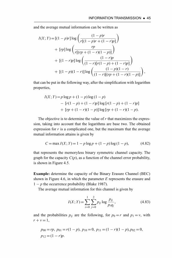
INFORMATION TRANSMISSION • 45
and the average mutual information can be written as
I (X ; Y )= [(1− p)r] log(
(1− p)r
r[(1− p)r + (1− r)p]
)
+ [rp] log(
rp
r[(rp+ (1− r)(1− p)]
)
+ [(1− r)p] log(
(1− r)p
(1− r)[r(1− p)+ (1− r)p]
)
+ [(1− p)(1− r)] log(
(1− p)(1− r)
(1− r)[(rp+ (1− r)(1− p)]
),
that can be put in the following way, after the simplification with logarithmproperties,
I (X ; Y )= p log p+ (1− p) log (1− p)
− [r(1− p)+ (1− r)p] log [r(1− p)+ (1− r)p]
+ [rp+ (1− r)(1− p)] log [rp+ (1− r)(1− p).
The objective is to determine the value of r that maximizes the expres-sion, taking into account that the logarithms are base two. The obtainedexpression for r is a complicated one, but the maximum that the averagemutual information attains is given by
C=max I (X ; Y )= 1− p log p+ (1− p) log (1− p), (4.82)
that represents the memoryless binary symmetric channel capacity. Thegraph for the capacity C(p), as a function of the channel error probability,is shown in Figure 4.5.
Example: determine the capacity of the Binary Erasure Channel (BEC)shown in Figure 4.6, in which the parameter E represents the erasure and1− p the occurrence probability (Blake 1987).
The average mutual information for this channel is given by
I (X ; Y )=1∑
i=0
2∑j=0
pij logpij
piqj, (4.83)
and the probabilities pij are the following, for p0= r and p1= v, withr + v= 1,
p00= rp, p01= r(1− p), p10= 0, p11= (1− r)(1− p), p02= 0,
p12= (1− r)p.
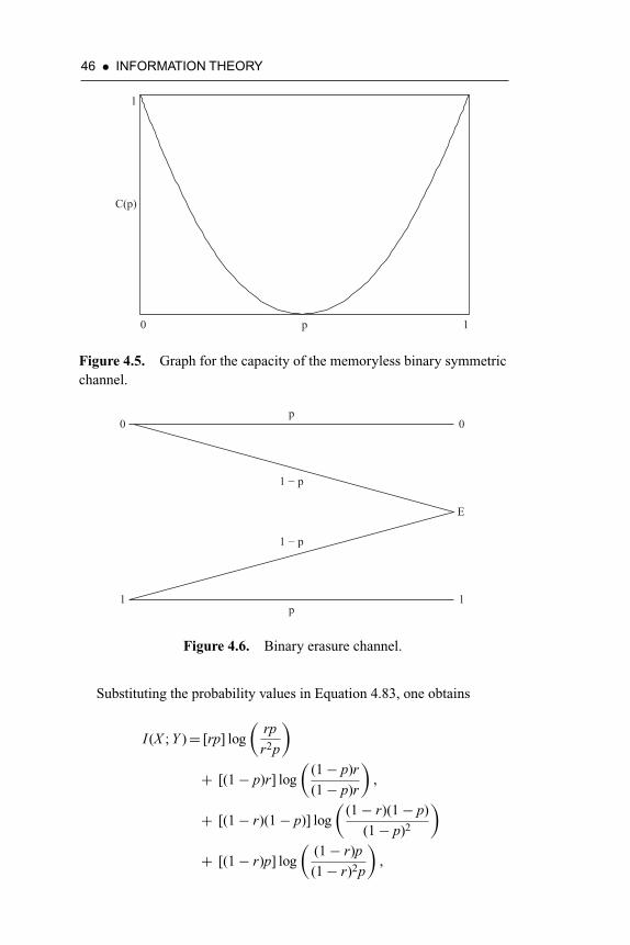
46 • INFORMATION THEORY
10
1
C(p)
p
Figure 4.5. Graph for the capacity of the memoryless binary symmetricchannel.
0
1
0
1
p
p
1 − p
1 − p
E
Figure 4.6. Binary erasure channel.
Substituting the probability values in Equation 4.83, one obtains
I (X ; Y )= [rp] log(
rp
r2p
)
+ [(1− p)r] log(
(1− p)r
(1− p)r
),
+ [(1− r)(1− p)] log(
(1− r)(1− p)
(1− p)2
)
+ [(1− r)p] log(
(1− r)p
(1− r)2p
),

INFORMATION TRANSMISSION • 47
10
1
C(p)
p
Figure 4.7. Graph of the capacity for the binary erasure channel.
Simplifying the terms in the expression, gives
I (X ; Y )= p[r log r − (1− r) log (1− r)]= pH (r), (4.84)
in which H (r) is the entropy function.Because p is determined, I (X ; Y ) is maximized by the choice of a
value for r that produces the highest H (r), that is, r= 1/2, for whichH (r)= 1. Therefore, the capacity of the binary erasure channel is sim-ply p. Figure 4.7 shows the graph for the capacity as a function of theprobability p.

CHAPTER 5
MULTIPLE ACCESS SYSTEMS
5.1 INTRODUCTION
The multiple access channel can be analyzed through the use of an infor-mation theoretic approach. In this type of communications system, severalusers transmit simultaneously to a common receiver. The main multiplex-ing strategies that fall in that category include frequency division multipleaccess (FDMA), time division multiple access (TDMA), and code divisionmultiple access (CDMA).
The main objective of the information theoretic approach of the multi-ple access channel is to find its capacity region, that is, the set of informationrates at which the simultaneous reliable communication of the messagesof each user is possible (Verdú 1989b).
The problem of finding the capacity region of a multiple access chan-nel can be traced to a pioneering work on two-way communication chan-nels by Shannon, in 1961 (Shannon 1961). A similar approach led tothe multi-way solution for the discrete memoryless channel (Ahlswede1971). The related problem of simultaneous communication from onesource to several receivers was proposed in 1971, and solutions weregiven to the cases of orthogonal, Gaussian, and compound channels (Cover1972).
The usual assumption for the Shannon channel was a strategic coopera-tion between the senders and the receiver. This approach changed in 1981,when the lack of synchronization was proven not to reduce the capacityregion for the multiple access channel (Cover, McEliece, and Posner 1981).Later it was shown, for the two-user case, that the only effect of frame asyn-chronism on the discrete memoryless channel is the removal of the convexhull operation from the expression of the capacity region.

50 • INFORMATION THEORY
The same result could be extended to the multiuser case and implies thatthe maximum achievable rate sum, or total capacity, of the memoryless mul-tiple access channel is never decreased by the lack of frame synchronism.This is a direct implication of the convexity property, because the rate sumof any convex combination of rate pairs is equal to the convex combinationof the respective rate sums (Hui and Humblet 1985).
Further study on the asynchronous Gaussian multiple access channelestablished the nonoptimality of the conventional receiver (independentdetection of the signals), which is a result of the additive component ofmultiple access interference (MAI). Fortunately for CDMA systems, inwhich the designer is allowed to choose a signal constellation with largebandwidth, the cross-correlations between the signals can be kept low forall relative delays and an acceptable performance can be achieved (Verdú1986).
A paper published in 1975 showed, by means of an example, that theuse of feedback could increase the capacity region of the multiple accessmemoryless channel. But the problem of determining the actual capac-ity region, when feedback is available, remained unsolved (Gaarder andWolf 1975). A point to be stressed here is that, despite the efforts of manyresearchers in the field, the capacity region of the multiterminal commu-nication channel remains, in general, unknown. A general formula for thecapacity of such channels is expressed by (Mandell and McEliece 1991).
The role of the memory in the multiple access environment was stressedin the article (Verdú 1989a). In fact, the study of asynchronous multipleaccess channels can be enriched with the theory of multiple access channelswith memory, in which the effect on the current symbol depends on theprevious state of the channel. The usual approach to the design of codesfor channels with memory has been the assumption of interleaving, whichprovides an interesting trade-off between decoding complexity and storagecapacity.
In one of the first works to suggest this technique, interleaving appearedas a type of time division multiplexing (Elliott 1965). The issue there wasthat interleaving could enhance the error-control effectiveness of error-correcting codes, when the separation between bits of a code word is onthe order of several hundred bits. The purpose of interleaving is to providerandomization, in order to mitigate potential burst errors.
There are many different types of channels that can be characterized bythe nature of errors that are generated between transmitter and receiver.On a bursty channel, given a burst of symbols, an interleaving schemecan be used to spread the errors to many codewords. A suitable error-correcting code could then be utilized to correct the remaining errors in

MULTIPLE ACCESS SYSTEMS • 51
each codeword. An optimum interleaver is then one which utilizes the leastamount of memory and has the smallest average delay between the inputand output of a symbol from the interleaver, besides providing the neces-sary randomization of the data.
The symbol-asynchronous Gaussian multiple access channel encom-passes many interesting models. The direct sequence spread spectrum mul-tiple access channel represents a possible application for some of thosemodels. The capacity region of the symbol-asynchronous Gaussian mul-tiple access channel was obtained recently (Verdú 1989b). However, fur-ther study is necessary to obtain the capacity region for the asynchronousGaussian multiple access channel with memory. This could be helpful inmodeling the wireless digital communications channel as introduced in thelast chapter.
Moreover, for channels with memory, frame asynchronism may drasti-cally reduce the capacity region and, in particular, the maximum achiev-able rate sum. A useful model for a channel with memory will beintroduced in the last section of this chapter and analyzed in some detail.
5.2 THE GAUSSIAN MULTIPLE ACCESSCHANNEL
The multiple access channel can be defined as a system in which Mtransmitters, Xi ∈Xi, simultaneously communicate to a common recei-ver, Y ∈Y . It is characterized by the transition probability matrixP(y|x1, · · · , xM ), which represents the probabilities associated with out-put y when the M inputs are x1, · · · , xM . The channel is assumed memo-ryless, and the alphabets are considered continuous sets. When the noiseaffecting the transmitted signals is considered Gaussian, the systems iscalled the Gaussian multiple access channel, which was studied in detailby (Wyner 1974).
The choice of Gaussian signals to convey information in the additiveGaussian channel is not a matter of chance. The use of a set of Gaussianwaveforms maximizes the mutual information for this kind of channel(Sommer 1966). The multiple access channel is shown in Figure 5.1.
In the following, a general idea on the computation of the capacity regionis presented. Consider that the output is Y =∑i Xi + Z , in which the Xi
are inputs and Z is a Gaussian noise random variable independent of theinputs, with variance σ 2
Z . The encoding constraint is that the messages,which are n-vectors, satisfy E[(1/n)||Xi||2]≤ σ 2
i .The Euclidean norm || · ||is used for the vectors in the preceding formula. Besides, one imposes the

52 • INFORMATION THEORY
YCHANNEL
XM
X2
X1
Figure 5.1. The multiple access channel.
additional condition that E[X 2i ]≤ σ 2
i , i= 1, . . . , M (Wyner 1974). In thefollowing, all logarithms are to the base two, which implies that informationrates, and capacities, are measured in bits.
The mutual information can be defined for the set of inputs and out-put as the difference between the output entropy H (Y ) and the noiseentropy H (Z)
I (X1, · · · , XM ; Y )
=H (Y )− H (Y |X1, · · · , XM ) (5.1)
=H (Y )− H (Z). (5.2)
Considering the independence between the inputs and the Gaussiannoise, the variance of the output can be written
V [Y ]=M∑
i=1
V [Xi]+ V [Z] (5.3)
≤M∑
i=1
σ 2i + σ 2
Z . (5.4)
Therefore, the mutual information is bounded by
I (X1, · · · , XM ; Y )≤ 1
2log 2πe
(M∑
i=1
σ 2i + σ 2
Z
)
− 1
2log 2πeσ 2
Z
= 1
2log
(∑Mi=1 σ 2
i + σ 2Z
σ 2Z
)(5.5)
= 1
2log (1+ S2)
�=C. (5.6)

MULTIPLE ACCESS SYSTEMS • 53
in which the total signal-to-noise ratio (SNR) is defined as
S2=∑M
i=1 σ 2i
σ 2Z
. (5.7)
Furthermore,
I (Xi; Y |X1, · · · , Xi−1, Xi+1, · · · , XM )
=H (Y |Xi)− H (Y |X1, · · · , XM ) (5.8)
for i= 1, · · · , M (5.9)
which is bounded as
I (Xi; Y |X1, · · · , Xi−1, Xi+1, · · · , XM )
≤ 1
2log
(σ 2
i + σ 2Z
σ 2Z
)
= 1
2log (1+ s2
i )�=Ci (5.10)
for i= 1, · · · , M
in which s2i is
s2i =
σ 2i
σ 2Z
. (5.11)
A multiuser discrete multiple access channel satisfies
Ri ≤ I (Xi; Y |X1, · · · , Xi−1, Xi+1, · · · , XM ),
for i= 1, · · · , M
R1 + · · · + RM ≤ I (X1, · · · , XM ; Y ) (5.12)
in which the set of Ri represents the transmission rates for M independentinput signals Xi. The output signal is Y . The boundary of this region iscalled the convex hull.
Example: the set of all achievable rates must lie inside the region defined bythe inequalities R1 + · · · + RM ≤C and Ri ≤Ci, as depicted in Figure 5.2,for the case of two users.
For the case of three users, the set of equations above define an upperbound on the capacity, because other constraints can be imposed on thepartial sums of transmission rates.
The channel capacity, or the maximum possible transmission rate, canonly be attained on the convex hull, or contour surface. Thus time-sharingcould be necessary to achieve some of the points in the capacity region, for

54 • INFORMATION THEORY
0
R1 + R2 = C
R2C2
C1
R1
Figure 5.2. Capacity region for the Gaussian multiple access channel,M = 2.
instance if Ci=C (Bierbaum and Wallmeier 1979). This model assumescooperative users, which can be translated into a time-sharing environ-ment.The transmission of information without any prearrangement betweenthe users results in a degradation of the capacity region (Sommer 1966),which can be minimized with the use of multiplexing techniques suchas CDMA.
5.3 THE GAUSSIAN CHANNEL WITHRAYLEIGH FADING
Consider that the output is Y =∑i riXi + Z , in which the Xi are the trans-mitted signal, Z is a Gaussian noise random variable independent of theinputs, with variance σ 2
Z , and ri are the attenuation coefficients associatedwith the fading channel. The channel is assumed memoryless, and thealphabets are considered continuous sets.
The choice of Gaussian signals to convey information in the additiveGaussian channel does not optimize the transmission rate any more. Theaccuracy of a simple approximation to the capacity of a fading, additiveGaussian noise channel is discussed for the single user case. The specialcase of Rayleigh fading is considered in greater detail and the signal dis-tribution that yields capacity for this case is found.
The random variables ri are the attenuation parameters defined inChapter 2, which are assumed to follow a Rayleigh distribution given by
pR(r)= r
γ 2 e− r2
2γ 2 u(r). (5.13)

MULTIPLE ACCESS SYSTEMS • 55
The output is not guaranteed to be Gaussian, for a Gaussian input, inthe fading channel. This is the reason for not assuming an input Gaussiandistribution in the first hand. The product of the signal versions and theattenuation factors yield a distribution that is not Gaussian, in the generalcase, for the received signal.
This poses a problem for computing the capacity region: The capacityis obtained by maximizing the mutual information over all the input distri-butions and this is achieved, for the Gaussian channel, only by producing aGaussian output (Shannon 1948). Thus, in order to attain the capacity onehas to “Gaussianize” the output by choosing a suitable distribution for theset of input signals.
A fading additive Gaussian noise channel is assumed to have an output ofthe form Y =RX + Z in which: N is a Gaussian random variable with meanzero and variance σ 2
Z , that is, N ∼N (0, σ 2Z ); X is a signal random variable
with density function pX (x) and variance σ 2X ; R is a positive valued random
variable with density function pR(r) and E[R2]= 2γ 2; Y is the receivedrandom variable. It is assumed that X and therefore Y has mean zero. Thecapacity of this channel has been determined (Ericson 1970) as:
C(s2)=ER
[1
2log (1+ R2s2)
], s2= σ 2
X /σ 2Z
=∫ ∞
0pR(r)
1
2log (1+ r2s2)dr, (5.14)
in which the units will be bits per channel use and the parameter s2 willbe referred to as SNR. The equation results from the consideration of theparametric equations defining the reliability function for random codingfor this channel and is valid for any positive valued random variable.
It is of interest here to know how this expression is related to the equation
C(s2)= 1
2log (1+ γ 2s2), (5.15)
which might be easier to use in many situations.From the convexity of the logarithm function and Jensen’s inequality
(Blahut 1987) it is clear that for all SNRs, s2, C(s2)≤C(s2). The magnitudeof the difference C(s2)− C(s2) will be shown, graphically, to be smallfor the case of a Rayleigh fading distribution. Implicit in the form of thecapacity expression is the fact that Y should be a Gaussian random variableto achieve capacity. Consequently U =RX should be a Gaussian randomvariable.
The question of determining the distribution of X , for a given distribu-tion of R to yield U a Gaussian distribution is considered. It is noted that
56 • INFORMATION THEORY
since U and R are correlated with unknown joint distribution, this prob-lem is quite different from the usual transformation problem for randomvariables. It is solved for the case of R Rayleigh distributed. The generalproblem seems difficult.
From the form of the equation for the capacity of the channel, it isargued that to achieve capacity, Y must be a zero mean Gaussian randomvariable. For a given fading random variable R, the signal random variable Xshould be chosen so that U =RX is Gaussian. Since U and R are correlatedit does not seem a simple matter to compute the distribution of X =U/R,using the standard techniques.
Likewise, it does not seem a simple matter to compute I (X , Y ) andthe maximizing distribution to achieve capacity, making the technique of(Ericson 1970) the more interesting.
Example: for the case of R a Rayleigh distributed random variable withdensity the distribution of X can be achieved in the following manner.
Since R and X are, by assumption, independent and Y − N =U =RX ∼N (0, σ 2
U ) , as discussed, then X has a zero mean and a symmetric distri-bution. Odd moments of U and X are zero and E[X 2k ]=E[U 2k ]/E[R2k ].The required moments are readily computed as
E[R2k ]= k!γ 2k E[U 2k ]= (2k)!2k k! σ
2kU , (5.16)
and so
E[X 2k ]= E[U 2k ]
E[R2k ]=(
2k
k
)(σ√2γ
)2k
, k = 1, 2, 3, · · · . (5.17)
Let a= σ/(√
2γ ). Let pX (x) be the density of X and φX (v) the characteristicfunction. The series expansion of φX (v) is
φX (v)=∞∑
k=0
(− 1)k E[X 2k ]
(2k)!
=∞∑
k=0
(− 1)k
(2kk
)(2k)!
=∞∑
k=0
(− 1)k (av)2k
(k!)2
(5.18)
This series is identified as (Abramowitz and Stegun 1965, p. 360) J0(av)in which J0( · ) is a Bessel function of the first kind and zeroth order. The

MULTIPLE ACCESS SYSTEMS • 57
corresponding density function is then given as (Oberhettinger 1990)
pX (x) = 1
2π
∫ ∞−∞
J0(av)e−jvxdv
= 1
π ((2a)2 − x2)1/2 , |x|< 2a(5.19)
Thus for the random variable X with this density, R with the Rayleighdensity, U =RX has the required Gaussian density N (0, σ 2
U ). While theabove technique is of interest, since success depends on the identificationof an infinite series, it does not lend itself to generalization.
The effect of fading has been removed from the final expression for thecapacity at a certain cost. In order to counterbalance the stochastic atten-uation, it is necessary to design a circuit that provides the transformationof random variables necessary at the transmission end. It is not certain, atthis point, that this can be achieved in general for any type of fading.
In physical terms, the introduction of fading in the channel decreasesthe noise margin of the system. Thus, the detection threshold remains con-strained to a smaller region near the origin, for the case of binary commu-nications. If the input distribution cannot be altered, it is possible to defineanother transmission rate, which will fall short of being the optimum in thiscase. The trade-off assumed for attaining the full capacity of the systemresides in the design of a circuit to transform the input signal and shape itsprobability density function (pdf) accordingly.
The capacity evaluated by Ericson (1970) can be interpreted as anaverage channel capacity, as defined by Lee (1990), or as analyzed byDobrushin (1961). The concept of average or mean capacity can be provenuseful, anyway, and has been successfully applied to the case of dynamicallocation of users (Alencar and Blake 1993a).
In order to complete the investigation, in light of the results of Eric-son, one presents the derivation of the formula for the average capac-ity for the single user case, beginning with the general expression below(Ericson 1970)
C=ER
[1
2log (1+ R2s2)
](5.20)
in which s2= σ 2X /σ 2
Z is the SNR and E[ · ] represents the expected valuefunctional.
Example: introducing the Rayleigh pdf, from Equation 5.13, into the pre-vious formula gives
C= 1
2
∫ ∞−∞
log (1+ r2s2)r
γ 2 e− r2
2γ 2 u(r)dr. (5.21)

58 • INFORMATION THEORY
The last equation can be simplified by the application of a known theo-rem of probability (Blake 1987), leading to
C= log e
4γ 2
∫ ∞0
log (1+ ξs2)e− ξ
2γ 2 dξ , (5.22)
which can be solved by standards methods, yielding
C=− log e
2Ei(− 1
2γ 2s2
)e
12γ 2s2 (5.23)
in which the Exponential Integral function is defined by
Ei(x)=∫ x
−∞et
tdt, x < 0. (5.24)
Concluding this section, Figure 5.3 illustrates a comparison betweenFormulas 5.15 and 5.23, in the single user case, for three values of thefading parameter γ . The dotted curves represent the average capacity, foreach value of the parameter.
C0.5
1.0
2.0
SNR3020100-10
0
6
5
4
3
2
1
Capacity, nats per channel use
Figure 5.3. Average and actual capacity, for γ = 0.5, 1.0, and 2.0.

MULTIPLE ACCESS SYSTEMS • 59
5.4 THE NONCOOPERATIVE MULTIPLEACCESS CHANNEL
The noncooperative channel has asynchronous multiplexing, which im-plies that the M information sources transmit through a common mediumwithout any prearrangement among themselves (Sommer 1966). There-fore, all components of the received signal are statistically independent,and so perform as interference with respect to any other given signal.
For the conditions mentioned, a slight generalization of a former workcan be attempted (Sommer 1966). Based on the results stated in Shannon(1948), the mutual information between the set of inputs and the output,for the noncooperative additive Gaussian noise channel, can be written as
I (X1, · · · , XM ; Y )=H (Y )− H (Y − G) (5.25)
in which
G=M∑
i=1
Xi. (5.26)
This leads to the already evaluated expression
I (X1, · · · , XM ; Y )=H (Y )− H (Z) (5.27)
bounded as
I (X1, · · · , XM ; Y )≤ 1
2log 2πe
(M∑
i=1
σ 2i + σ 2
Z
)
− 1
2log 2πeσ 2
Z
= 1
2log
(∑Mi=1 σ 2
i + σ 2Z
σ 2Z
)(5.28)
= 1
2log (1+ S2)
�=C. (5.29)
By the same token, one can compute the individual mutual information
I (Xi; Y )=H (Y )− H (Y − Xi) (5.30)
≤ 1
2log 2πe
(σ 2
Z S2 + σ 2Z
)− 1
2log 2πe
(σ 2
Z S2i + σ 2
Z
)(5.31)
in which the interference to noise ratio (INR) is defined as
S2i =
∑Mj=1 j �=i σ
2j
σ 2Z
. (5.32)

60 • INFORMATION THEORY
Rearranging the terms in 5.31 gives
I (Xi; Y )≤ 1
2log(
S2 + 1
S2i + 1
)�=Ci. (5.33)
The capacity region forms a square in two dimensions, a parallelepipedfor three sources, and a hyper-parallelepiped for more than three sources.It can be seen that the hyperplane defined by expression 5.29 never touchesthe contour surface, which means that the capacity of the noncooperativechannel is given by the sum of the individual rates,
C=M∑
i=1
Ci (5.34)
or
C= 1
2
M∑i=1
log(
S2 + 1
S2i + 1
)(5.35)
which can be put in the form
C= 1
2log
(M∏
i=1
S2 + 1
S2i + 1
). (5.36)
Example: the last expression is maximized when all the transmitters carrythe same power, that is, σ 2
i = σ 2. This assumption simplifies the expressionof the INR to
S2i =
M − 1
MS2 (5.37)
and also simplifies the formula for the channel capacity
C= 1
2log
(S2 + 1
M−1M S2 + 1
)M
(5.38)
or
C= 1
2log(
M (S2 + 1)
M (S2 + 1)− S2
)M
. (5.39)
Example: an interesting result can be obtained by taking the limit of thecapacity when the number of sources goes to infinity. First, the formula isrearranged to
C= 1
2log(
1− S2
M (S2 + 1)
)−M
(5.40)

MULTIPLE ACCESS SYSTEMS • 61
or, by noticing that S2=Ms2
C= 1
2log(
1− s2
M (s2 + 1/M )
)−M
. (5.41)
Now, using the known property of limits
limM→∞
(1+ 1
M
)M
= e (5.42)
one obtains finally
C∞= log e
2. (5.43)
Thus, for a large number of transmitters the capacity assumes the valuelog e/2, which is bounded and low if compared to the capacity that can beachieved with the cooperative approach between the users. This must alsobe compared to the single user capacity, obtained by allowing M = 1 inexpression 5.41
C= 1
2log (1+ s2) (5.44)
which is unbounded with respect to the SNR. The capacity region forthe noncooperative channel can be seen in Figure 5.4, for two users, as arectangle inside the diamond shaped capacity region for the cooperativechannel, evaluated by Wyner (1974). The points C1, C ′1, C2, and C ′2 aredefined below
C1= 1
2log
(1+ σ 2
1
σ 22 + σ 2
Z
)C ′1=
1
2log
(1+ σ 2
1
σ 2Z
)(5.45)
0
R1 + R2 = C
R2C'2C2
C'1
C1
R1
Figure 5.4. Capacity region for the noncooperative channel, M = 2.

62 • INFORMATION THEORY
and
C2= 1
2log
(1+ σ 2
2
σ 21 + σ 2
Z
)C ′2=
1
2log
(1+ σ 2
2
σ 2Z
). (5.46)
As the number of users increases towards infinity the capacity regionshrinks, and the channel capacity converges to a given value. There is noway to increase the capacity of the noncooperative channel by increasingthe power of the transmitted signals. The limiting capacity C∞ becomesindependent of the SNR, as the number of senders goes to infinity. A possi-bility left to boost the capacity is by an increase in the available bandwidth.Spread spectrum techniques could prove useful in this case.
5.5 MULTIPLE ACCESS IN A DYNAMICENVIRONMENT
The selection of the more appropriate multiple access technique, for agiven communications problem, depends on the channel characteristics.This section describes and analyzes a model for the Gaussian multipleaccess channel, in which the addition of new users is governed by a renewalprocess. An information theoretic approach is attempted, in order to findthe set of transmission rates at which the reliable communication of themessages of each user is possible.
The problem of finding the capacity region of a multiple access chan-nel can be linked to a seminal work by Shannon on two-way commu-nication channels in 1961 (Shannon 1961). A usual assumption for theShannon model is a strategic cooperation between the senders and thereceiver.
The next section presents a different approach for the analysis ofthe multiple access channel. Instead of relying on static models forthe channel, a dynamic structure is proposed and analyzed. The non-cooperative model in which the users compete for the channel resourcesis assumed. The access, or addition of new users to the channel, is gov-erned by a Markovian process and the multiple access interference(MAI) is assumed proportional to the number of active users (Kleinrock1975). This model assumes a variable assignment for the allocation ofusers in the channel, which is a reasonable assumption for CDMAsystems.

MULTIPLE ACCESS SYSTEMS • 63
5.6 ANALYSIS OF THE CAPACITY FOR AMARKOVIAN MULTIPLE ACCESS CHANNEL
Most models proposed for the multiple access channel assume that thenumber of users in the channel is fixed—but, in most cases, it is actually arandom variable, governed by a distribution of probabilities. The channelcapacity, for many channels, varies with the real time allocation of users.For instance, the capacity for the noncooperative model of accessibility isa function of the number of users which contribute to the multiple accessinterference (MAI). In the memoryless noncooperative channel the capac-ity decreases as more users are introduced, reaching a fixed value as thisnumber increases to infinity (Alencar 1992b; Sousa 1989).
In order to account for the effect of a changing environment, with theusers dropping in and out of the channel, a new model is proposed. Considera Gaussian channel with k users. The variance of the MAI in the channel isassumed to be kσ 2
X plus some background Gaussian noise of σ 2Z . Thus, the
total noise variance depends on how many users are on the channel. It ismeant to reflect a multiuser channel with other user interference modeledby Gaussian noise. Now suppose the channel is in state k if there are kusers are on the channel, and a Markovian transition regime is imposed.
One model that might be interesting is a birth–death model, in whichtransitions occur only between adjacent states—so from state k you can goto either k + 1 or k − 1, with certain probabilities. Thus, for example, in asynchronous system this might reflect the model in which the probabilityof more than one user entering or leaving the system in a given data bit isnegligible. The steady state probabilities are not difficult to compute and aformula for the average channel capacity for the model can be found.
The channel with extrinsic memory can be thought of as a dynamicsystem, governed by a birth–death process, with a variable number of activeusers and implying a dynamic capacity—contrary to the classical staticcapacity that assumes a fixed number of users. It can be seen as an infinitestate channel (ISC), as opposed to the finite state models for channels foundin the literature (Gilbert 1960; Fritchman 1967). In this new approach, thechannel capacity changes as the number of users changes in a dynamicfashion. This last quantity is considered a stochastic process, and has anunderlying Markov chain of states (Kleinrock 1975).
A transition probability matrix P={pij} governs the behavior of thechannel accessibility. The transition probabilities are obtained from theMarkov model depicted in Figure 5.5, in which αk and βk are the birth anddeath parameters, respectively. The channel will be called the Alpha-Beta
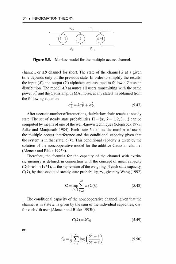
64 • INFORMATION THEORY
k +1kk – 1
αk–1 αk
βk+1βk
Figure 5.5. Markov model for the multiple access channel.
channel, or AB channel for short. The state of the channel k at a giventime depends only on the previous state. In order to simplify the results,the input (X ) and output (Y ) alphabets are assumed to follow a Gaussiandistribution. The model AB assumes all users transmitting with the samepower σ 2
X and the Gaussian plus MAI noise, at any state k , is obtained fromthe following equation
σ 2k = kσ 2
X + σ 2N . (5.47)
After a certain number of interactions, the Markov chain reaches a steadystate. The set of steady state probabilities �={πk |k = 1, 2, 3 . . .} can becomputed by means of one of the well-known techniques (Kleinrock 1975;Adke and Manjunath 1984). Each state k defines the number of users,the multiple access interference and the conditional capacity given thatthe system is in that state, C(k). This conditional capacity is given by thesolution of the noncooperative model for the additive Gaussian channel(Alencar and Blake 1993b).
Therefore, the formula for the capacity of the channel with extrin-sic memory is defined, in connection with the concept of mean capacity(Dobrushin 1961), as the supremum of the weighing of each state capacity,C(k), by the associated steady state probability, πk , given by Wang (1992)
C= sup{πk }
M∑k=1
πk C(k). (5.48)
The conditional capacity of the noncooperative channel, given that thechannel is in state k , is given by the sum of the individual capacities, Cik ,for each i-th user (Alencar and Blake 1993b),
C(k)= kCik (5.49)
or
Ck = 1
2
k∑i=1
log(
S2 + 1
S2i + 1
)(5.50)

MULTIPLE ACCESS SYSTEMS • 65
in which S2 represents the total SNR. The expression can be put in the form
Ck = 1
2log
(k∏
i=1
S2 + 1
S2i + 1
). (5.51)
The last expression reaches a maximum when all the transmitters carrythe same power, that is, σ 2
i = σ 2X . This assumption simplifies the formula
of the interference to noise ratio (INR) to
S2i =
k − 1
kS2 (5.52)
and also simplifies the formula for the channel conditional capacity, giving
Ck = 1
2log
(S2 + 1
k−1k S2 + 1
)k
(5.53)
or
Ck = 1
2log(
k(S2 + 1)
k(S2 + 1)− S2
)k
, (5.54)
which can be further simplified by noticing that the total SNR is S2= ks2,in which s2= σ 2
X /σ 2Z .
Two special cases for the AB model are treated here. First, the casein which the birth and death parameters are considered constant for anystate, and the access is unrestricted. Second, the case in which the usersare discouraged by the amount of noise in the system. This occurs becauseevery new user can be thought to degrade the system to a certain extent,by decreasing the SNR. For the first case, αk = λ and βk =μ. For thesecond case, αk = λ/(k + 1) and βk =μ, in which λ and β are fixedprobabilities.
Example: the first case produces a Geometric distribution for the proba-bilities.
This distribution shows the likelihood of being in a certain state in thelong run, after the transient dies out and is given by the equation
pk = (1− ρ)ρk , k = 0, 1, 2, . . . , for ρ < 1 (5.55)
in which ρ= λ/μ is usually called the utilization factor of the system.For the Geometric distribution considered, the statistical mean is given
by ρ/(1− ρ) and the variance by ρ/(1− ρ)2. The probability of finding
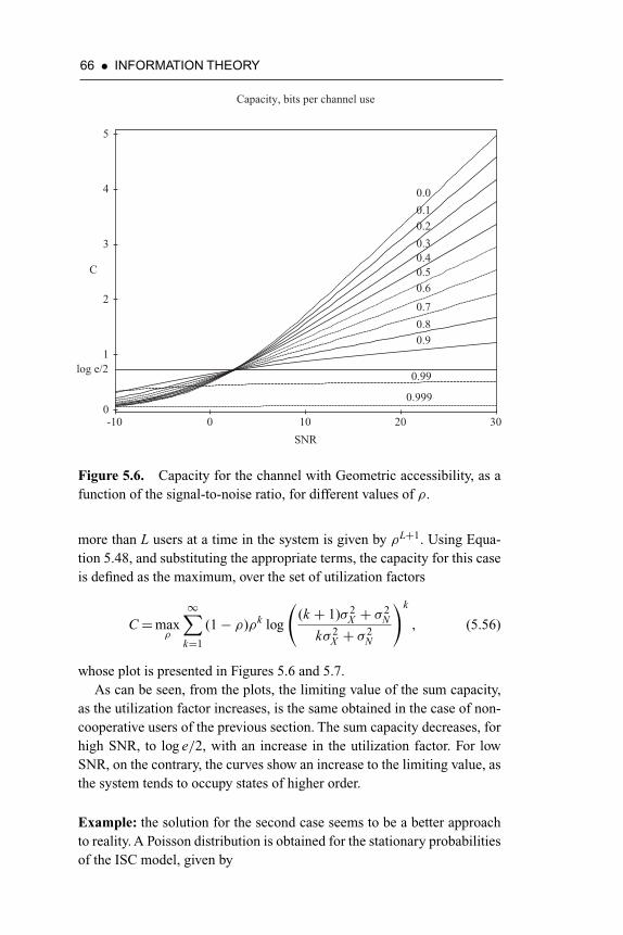
66 • INFORMATION THEORY
C
log e/2
0.00.10.20.30.40.50.60.70.80.9
0.99
0.999
SNR3020100-10
0
5
4
3
2
1
Capacity, bits per channel use
Figure 5.6. Capacity for the channel with Geometric accessibility, as afunction of the signal-to-noise ratio, for different values of ρ.
more than L users at a time in the system is given by ρL+1. Using Equa-tion 5.48, and substituting the appropriate terms, the capacity for this caseis defined as the maximum, over the set of utilization factors
C=maxρ
∞∑k=1
(1− ρ)ρk log
((k + 1)σ 2
X + σ 2N
kσ 2X + σ 2
N
)k
, (5.56)
whose plot is presented in Figures 5.6 and 5.7.As can be seen, from the plots, the limiting value of the sum capacity,
as the utilization factor increases, is the same obtained in the case of non-cooperative users of the previous section. The sum capacity decreases, forhigh SNR, to log e/2, with an increase in the utilization factor. For lowSNR, on the contrary, the curves show an increase to the limiting value, asthe system tends to occupy states of higher order.
Example: the solution for the second case seems to be a better approachto reality. A Poisson distribution is obtained for the stationary probabilitiesof the ISC model, given by

MULTIPLE ACCESS SYSTEMS • 67
C
log e/2
SNR=30dB
SNR=20dB
SNR=10dB
SNR=0dBSNR=-10dB
Utilization factor10.80.60.40.2
0
5
4
3
2
1
Capacity, bits per channel use
Figure 5.7. Capacity for the channel with Geometric accessibility, as afunction of the utilization factor, for different values of the signal-to-noiseratio.
pk = ρk
k! e−ρ , k = 0, 1, 2, . . . (5.57)
with mean and variance equal to ρ.The capacity, therefore, is given by the maximum, over the range of
utilization factors, of the following formula
C=maxρ
∞∑k=1
ρk
k! e−ρ log
((k + 1)σ 2
X + σ 2N
kσ 2X + σ 2
N
)k
. (5.58)
The results are shown in Figures 5.8 and 5.9 as a function of the SNRand utilization factor, respectively. Figure 5.9, in particular, gives a goodexample of the system behavior as the utilization factor increases. It canbe seen that, as the distribution becomes more uniform, the sum capacitytends to the already computed limit log e/2. As the factor increases thereis a more pronounced tendency for the occupation of higher states in theMarkov chain.
Several models were described in this chapter. The first modeled thecase when the users acknowledge a certain protocol for transmission andcooperate to achieve the maximum transmission rates. In the second model,the users do not cooperate, in the sense that they transmit their signals
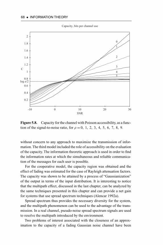
68 • INFORMATION THEORY
C
SNR
01
2
3
45
log e/2
0 302010-10
2
1.8
1.6
1.4
1.2
1
0.8
0.6
0.4
0.2
Capacity, bits per channel use
Figure 5.8. Capacity for the channel with Poisson accessibility, as a func-tion of the signal-to-noise ratio, for ρ= 0, 1, 2, 3, 4, 5, 6, 7, 8, 9.
without concern to any approach to maximize the transmission of infor-mation. The third model included the role of accessibility on the evaluationof the capacity. The information theoretic approach is used in order to findthe information rates at which the simultaneous and reliable communica-tion of the messages for each user is possible.
For the cooperative model, the capacity region was obtained and theeffect of fading was estimated for the case of Rayleigh attenuation factors.The capacity was shown to be attained by a process of “Gaussianization”of the output in terms of the input distribution. It is interesting to noticethat the multipath effect, discussed in the last chapter, can be analyzed bythe same techniques presented in this chapter and can provide a net gainfor systems that use spread spectrum techniques (Alencar 1992a).
Spread spectrum thus provides the necessary diversity for the system,and the multipath phenomenon can be used to the advantage of the trans-mission. In a real channel, pseudo-noise spread spectrum signals are usedto resolve the multipath introduced by the environment.
Two problems of interest associated with the closeness of an approx-imation to the capacity of a fading Gaussian noise channel have been
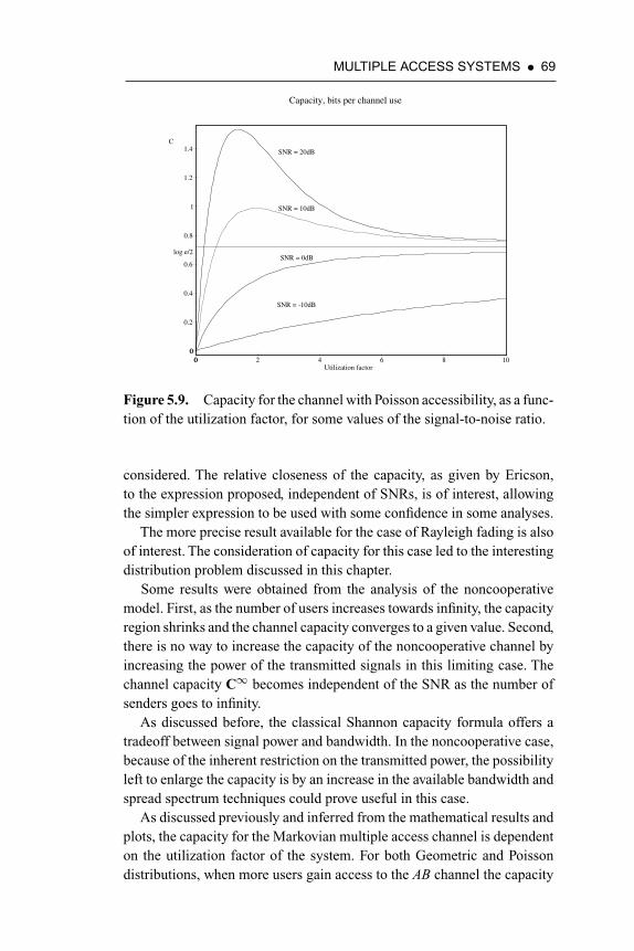
MULTIPLE ACCESS SYSTEMS • 69
C
SNR = 20dB
SNR = 10dB
SNR = 0dB
SNR = -10dB
log e/2
Utilization factor0 1086420
0
1.4
1.2
1
0.8
0.6
0.4
0.2
0
Capacity, bits per channel use
Figure 5.9. Capacity for the channel with Poisson accessibility, as a func-tion of the utilization factor, for some values of the signal-to-noise ratio.
considered. The relative closeness of the capacity, as given by Ericson,to the expression proposed, independent of SNRs, is of interest, allowingthe simpler expression to be used with some confidence in some analyses.
The more precise result available for the case of Rayleigh fading is alsoof interest. The consideration of capacity for this case led to the interestingdistribution problem discussed in this chapter.
Some results were obtained from the analysis of the noncooperativemodel. First, as the number of users increases towards infinity, the capacityregion shrinks and the channel capacity converges to a given value. Second,there is no way to increase the capacity of the noncooperative channel byincreasing the power of the transmitted signals in this limiting case. Thechannel capacity C∞ becomes independent of the SNR as the number ofsenders goes to infinity.
As discussed before, the classical Shannon capacity formula offers atradeoff between signal power and bandwidth. In the noncooperative case,because of the inherent restriction on the transmitted power, the possibilityleft to enlarge the capacity is by an increase in the available bandwidth andspread spectrum techniques could prove useful in this case.
As discussed previously and inferred from the mathematical results andplots, the capacity for the Markovian multiple access channel is dependenton the utilization factor of the system. For both Geometric and Poissondistributions, when more users gain access to the AB channel the capacity

70 • INFORMATION THEORY
increases up to a point in which it reaches a maximum. From this point on,if the number of users entering the channel is proportionately larger thanthe number of drop outs, the capacity begins to decrease. The capacity willeventually reach zero as the utilization factor increases to the limit. In thecase of a Geometrically distributed accessibility, the maximum capacity isachieved for a ρ= 0.97. The maximum value of ρ is one.
For the Poisson model the maximum is reached for ρ= 1.3, approx-imately. There is no limit for ρ if this distribution is used. The Poissondistribution models the case in which the incoming users are discouragedby the amount of noise in the system. As the SNR decreases, more usersabandon the channel. Both the Geometric and Poisson models result incapacities that are upper bounded by the capacity of the noncooperativechannel, with fixed assignment, as the number of users go to infinity (Alen-car and Blake 1993b).
This model is suitable for describing the properties of systems thatpresent a variable assignment for user allocation, as is the case with CDMAtechniques.

CHAPTER 6
CODE DIVISION MULTIPLE
ACCESS
6.1 INTRODUCTION
This chapter presents some of the main characteristics of spread spectrumsystems, including the indication of possible types of interference, anti-jamming advantages of the technique in terms of signal-to-noise (SNR)ratio and possible applications of the techniques. The usefulness of spreadspectrum to overcome interference is stressed. Among others, the mainsources of interference are multipath, multiple media, multiple user, andmultiple cell (Viterbi 1991).
The first developments using concepts related with the current tech-niques of spread spectrum occurred in the mid-forties, and the applicationsinvolved military problems (Scholtz 1982). The techniques acquired greatpopularity in the communications community, for the last 20 years, sincethe papers on the subject began to appear after two decades of secrecy dueto military interests.
The main feature of spread spectrum signals is related to their band-widths, which are much larger than those assigned to baseband or mod-ulated signals. The way in which the spectrum is spread is essential, andis often realized by a code that is independent of the transmitted data.The receiver needs a replica of the code, synchronized in time, in order torecover the data.
The spreading process introduces a great deal of redundancy in thetransmitted signal. This allows the receiver to suppress part of the interfer-ence embedded in the signal, which is the chief advantage of the process.
It is possible to devise other advantages of the spread spectrum systemsin relation to personal communications (Pickholtz, Schilling, and Milstein1982; Scholtz 1982).
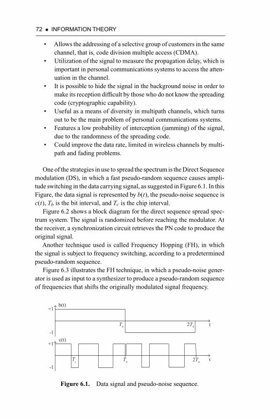
72 • INFORMATION THEORY
• Allows the addressing of a selective group of customers in the samechannel, that is, code division multiple access (CDMA).
• Utilization of the signal to measure the propagation delay, which isimportant in personal communications systems to access the atten-uation in the channel.
• It is possible to hide the signal in the background noise in order tomake its reception difficult by those who do not know the spreadingcode (cryptographic capability).
• Useful as a means of diversity in multipath channels, which turnsout to be the main problem of personal communications systems.
• Features a low probability of interception (jamming) of the signal,due to the randomness of the spreading code.
• Could improve the data rate, limited in wireless channels by multi-path and fading problems.
One of the strategies in use to spread the spectrum is the Direct Sequencemodulation (DS), in which a fast pseudo-random sequence causes ampli-tude switching in the data carrying signal, as suggested in Figure 6.1. In thisFigure, the data signal is represented by b(t), the pseudo-noise sequence isc(t), Tb is the bit interval, and Tc is the chip interval.
Figure 6.2 shows a block diagram for the direct sequence spread spec-trum system. The signal is randomized before reaching the modulator. Atthe receiver, a synchronization circuit retrieves the PN code to produce theoriginal signal.
Another technique used is called Frequency Hopping (FH), in whichthe signal is subject to frequency switching, according to a predeterminedpseudo-random sequence.
Figure 6.3 illustrates the FH technique, in which a pseudo-noise gener-ator is used as input to a synthesizer to produce a pseudo-random sequenceof frequencies that shifts the originally modulated signal frequency.
b(t)+1
-1Tb 2Tb t
c(t)+1
-1Tb 2Tb
Tc t
Figure 6.1. Data signal and pseudo-noise sequence.

CODE DIVISION MULTIPLE ACCESS • 73
Mixer Modulator Channel Demodulator Mixer
PN Generator Sync circuit PN Generator
Figure 6.2. Direct sequence spread spectrum system.
Modulator Mixer Channel Mixer Demodulator
PN Generator Synthesizer Synthesizer PN Generator
Figure 6.3. Frequency hopped spread spectrum system.
Buffer/Gate Modulator Channel Gate/Buffer Demodulator
PN Generator PN Generator Sync circuit
Figure 6.4. Spread spectrum using random time windows.
It is also possible to produce spread spectrum by transmitting bursts ofthe signal in random instants of time. This technique is known as TimeHopping (TH) and is illustrated in Figure 6.4.
Practical systems can combine the presented techniques, as is usuallythe case, to obtain certain properties. In a sense, the spread spectrum systemis an antithesis of the usual communication system. Because, in contrastto the usual system premises, it requires a very large bandwidth and a verylow power spectrum density for the transmitted signal.
Despite such advantages, the spread spectrum approach had some cri-tiques as quoted below:
The mystique of spread spectrum communications is such thatcommercial enterprises, as well as academics, are often attractedby the novelty and cleverness of the technique.Also, in small artifi-cially aided markets, there may be temporary economic advantages.

74 • INFORMATION THEORY
In the long run, though, it’s the author’s opinion that we must standback and question the wisdom of squandering a precious resourcesuch as bandwidth for reasons of expediency (Viterbi 1985).
6.2 FUNDAMENTALS OF SPREADSPECTRUM SIGNALS
It was mentioned in the last section that the spread spectrum techniquescan be used to protect the signal against jammers. The following discussesthe most common types of jammers, and how is it possible to attain thisobjective.
An attempt to classify the jammers is sketched below (Pickholtz, Schilling,and Milstein 1982; Cook and Marsh 1983):
• Partial band jammer. The interference is concentrated in a portionof the signal bandwidth.
• Partial time jammer, in which the intentional interference occurs inonly part of the transmission time. This can be accomplished by thetransmission of narrow pulses or impulses.
• Tone jammer, which concentrates its power in a single frequency.• Broad-band noise jamming. In this case the jammer tries to attack
the whole signal bandwidth. One possible approach is the genera-tion of a pseudo-noise sequence (PN) by the jammer.
• Repeater jamming. The jammer uses the very transmitted signal tocause the interference. This type of interference can produce a dele-terious influence on the signal spectrum that mimics the multipatheffect.
The vectorial, or signal space, approach is introduced here to explainhow spread spectrum can be used in parallel with other existing sys-tems and still protect the signals against interference to or from thosesystems (Wozencraft and Reiffen 1961). A data signal, with restricteddimensionality, is spatially expanded in such a way that prevents the degra-dation of the communication process by a limited power interferingsignal.
The classical digital transmission problem is the one in which bothtransmitter and receiver know the complete set of M waveforms xi(t), eachone with duration Tb seconds. The transmitter selects one of the M sig-nals at each Tb seconds, which yields a data rate of log2 (M )/Tb bits/s.If, for example, signal xj(t) is transmitted, the received signal over the
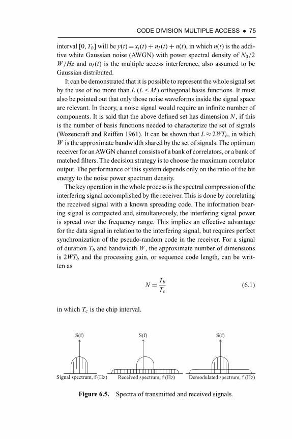
CODE DIVISION MULTIPLE ACCESS • 75
interval [0, Tb] will be y(t)= xj(t)+ nI (t)+ n(t), in which n(t) is the addi-tive white Gaussian noise (AWGN) with power spectral density of N0/2W /Hz and nI (t) is the multiple access interference, also assumed to beGaussian distributed.
It can be demonstrated that it is possible to represent the whole signal setby the use of no more than L (L≤M ) orthogonal basis functions. It mustalso be pointed out that only those noise waveforms inside the signal spaceare relevant. In theory, a noise signal would require an infinite number ofcomponents. It is said that the above defined set has dimension N , if thisis the number of basis functions needed to characterize the set of signals(Wozencraft and Reiffen 1961). It can be shown that L≈ 2WTb, in whichW is the approximate bandwidth shared by the set of signals. The optimumreceiver for anAWGN channel consists of a bank of correlators, or a bank ofmatched filters. The decision strategy is to choose the maximum correlatoroutput. The performance of this system depends only on the ratio of the bitenergy to the noise power spectrum density.
The key operation in the whole process is the spectral compression of theinterfering signal accomplished by the receiver. This is done by correlatingthe received signal with a known spreading code. The information bear-ing signal is compacted and, simultaneously, the interfering signal poweris spread over the frequency range. This implies an effective advantagefor the data signal in relation to the interfering signal, but requires perfectsynchronization of the pseudo-random code in the receiver. For a signalof duration Tb and bandwidth W , the approximate number of dimensionsis 2WTb and the processing gain, or sequence code length, can be writ-ten as
N = Tb
Tc(6.1)
in which Tc is the chip interval.
S(f)
Demodulated spectrum, f (Hz)
S(f)
Signal spectrum, f (Hz)
S(f)
Received spectrum, f (Hz)
Figure 6.5. Spectra of transmitted and received signals.
76 • INFORMATION THEORY
6.3 PERFORMANCE ANALYSIS OFCDMA SYSTEMS
The main areas of concern on multiple access systems are multiaccessinformation theory, collision resolution, and spread spectrum (Gallager1985). The approach followed by researchers on information theoreticmultiaccess takes into consideration the effects of noise and interference,neglecting the random arrivals of messages. On the other hand, research oncollision resolution focused primarily on the bursty arrivals of messagesand the interference between transmitters ignoring the noise component(Hui 1984a; Hui 1984b).
For multiaccess communication using spread spectrum several sourcescan transmit at the same time, using different modulating sequences, andeach will look like broadband noise to the others. Spread spectrum couldalso provide a solution to the problem of channel allocation.
One of the main problems in communications is the simultaneousallocation of multiple users to a channel. This must be accomplishedwithout severe degradation in the performance of the system. Three tech-niques have been proposed to attack the problem, as mentioned in theintroduction: FDMA, TDMA, and CDMA. The aim of the first two tech-niques is to separate the signals in frequency and time, respectively. Thethird one uses the properties of spread spectrum to separate the signals incode, that is, to modulate each message signal with a sequence selectedfrom a set of orthogonal sequences. Each user has its own address embed-ded in one of the code sequences (Cook et al. 1983). CDMA relies onthe ability of a spread spectrum system to reject independent interfer-ence by a factor approximately equal to its processing gain (Simon et al.1985).
An ideal system should combine the features of all the mentioned multi-ple access techniques, for example, the orthogonality of the TDMA systemleads to simultaneous achievability of single-user capacities by all users.In the case of FDMA or CDMA, this goal could be attained by a sufficientseparation of the frequencies in the former, and by the use of very largespreading factors in the latter (Cheng and Verdú 1991).
Multiple access techniques such as FDMA and TDMA are suscepti-ble to various types of interference, including jamming and multipath.FDMA also presents the intermodulation problem. On the other hand,TDMA must have all the users in perfect synchronism. Both FDMA andTDMA have their capacities limited by the available bandwidth. CDMAalso has its drawbacks. Interference caused by transmitters that are close tothe receiver cause the near-far problem. In a mobile environment, the near-far effect can be combated by the selection of sequences with very good
CODE DIVISION MULTIPLE ACCESS • 77
cross-correlation properties, as discussed in the next section, or by the useof adaptive power control (Schilling et al. 1991).
The second problem is the possibility of interference with existing sys-tems (Kavehrad and Ramamurthi 1987). Unlike the former techniques,CDMA has its capacity solely limited by the amount of interference intothe system, which allows any reduction in interference to be converteddirectly and linearly into and increase in capacity (Gilhousen et al. 1991).
As pointed out before, the use of spread spectrum allows new users toshare the spectrum with existing ones. CDMA is also interference limited,that is, the number of users that share the same spectrum and still maintainan acceptable performance is determined by the interference generatedby the set of remaining users. In CDMA systems, each user is given adistinct pseudo-random code. Hence, users in adjacent cells use the samebandwidth and therefore interfere, making a received signal appear noisieras the traffic increases in the system. The effect of the interfering energydepends on the processing gain of the spread spectrum technique.
Taking into account the adjacent cells interference, the total number ofusers M that can simultaneously access a given cell can be estimated fromthe following equation M = 3GP/8, in which GP is the processing gain.Thecomputation of M above assumes all users simultaneously transmitting.For a speech activity factor p and an interference increase factor λ theheuristic formula above can be adjusted to give the net number of users Uthat can access a given cell in a given time period (Schilling et al. 1991)
U = M
V (1+ λ). (6.2)
A more formal approach can be followed with the use of algebraic codingtheory and the definition of balanced codes. An (n, w, λ) binary balancedcode is a set of binary n-tuples, each of weight w, such that any two wordsagree in at most λ positions. If the maximum number of words in a balancedcode is U , it follows that (Blake and Mullin 1976; Chung and Kumar 1990)
U ≤
(n
λ+ 1
)(
wλ+ 1
) . (6.3)
In the last expression it is evident that the maximum of the autocor-relation function is given by w, and a good set of codes requires that theminimum distance, d = 2(w − λ), be kept at a maximum.
As implied above, spread spectrum systems are less subject to multipathsignal variations than conventional systems. In a direct sequence receiver,

78 • INFORMATION THEORY
if the reflected signal is delayed, compared to the direct signal, by more thanone code chip, the reflected signal is treated as any other uncorrelated inputsignal. The higher the code chip rate, for a particular system, the smallerits multipath problem. In the mobile environment, the result of multipathreception is that a moving receiver is subject to rapid fading and peaking ofits input signal as the the direct and reflected signals cancel and reinforceeach other. Stationary receivers are also subject to multipath due to thereflecting and refracting surfaces (Dixon 1984).
A few topics have interested researchers, industries, and users of CDMAsystems. The first one is the design of pseudo-noise sequences with goodautocorrelation and cross-correlation properties. The second concerns theevaluation of the system capacity, or how many users a CDMA system cansupport under given circumstances. The number of allocated users dictatesthe type of distribution to characterize the Multiple Access Interference(MAI). A large number of subscribers favor the Gaussian approximation.For a small number of subscribers, considering that the MAI is additivelycomposed of cross-correlations limited to a few chips of coincidence, themaximum interference is too small to apply the central limit theorem (Brady1991).
The evaluation of system performance can be done in two ways: usingthe average probability of error or computing the outage of the system. Theprobability of error is averaged over the ensemble of channels obtainedfrom the assumed model. The outage measures the probability of trans-mitting through a channel when the probability of error is greater then apredefined threshold. In the case of time-varying channel and stationaryterminal, outage indicates the fraction of time the terminal operates withan error probability above the limit. For the time-invariant channel andmobile terminal, outage indicates the fraction of building area in which theterminal can operate (Kavehrad and McLane 1987).
One interesting peculiarity of Direct Sequence Spread Spectrum (DSSS)is that error detection and correction may not be advisable in some applica-tions. This is due to the effect of the coding overhead, which increases thesignal apparent data transmission rate and reduces the available processinggain (Dixon 1984). On the other hand, a substantial improvement in thecapture performance of coded DSSS can be achieved, in comparison to anuncoded system. Capture phenomena characterize the ability of a receiverto successfully receive a packet, even though part or all of the packet arriv-ing at the receiver overlaps with the other packets. The basic mechanismfor capture is the ability of the receiver to synchronize with and lock onto one packet and subsequently reject other overlapping packets as noise(Soroushnejad and Geraniotis 1991).

CODE DIVISION MULTIPLE ACCESS • 79
In particular, time-frequency hopping modulation has a potential forapplication in those systems in which a large number of users, with widelyvariable distances or transmitted power, are to operate simultaneously in asingle link. Such systems tend to employ a simple code sequence, primarilyas an addressing medium, rather than to spread the spectrum specifically.This type of modulation is suitable for IWDC systems, in which randomaccess and discrete addressing are the main concerns. It also offers one ofthe few viable solutions to the near-far problem. By the use of synchro-nization the users can be programmed to transmit on different frequenciesas well as different times (Dixon 1984).
6.4 SEQUENCE DESIGN
Modeling a spread spectrum system implies the generation of randomsequences. Those sequences must exhibit the following properties: i) eachsignal in the set is easy to distinguish form a time-shifted version of itself;ii) each signal in the set is easy to distinguish from a time-shifted versionof every other signal in the set (Sarwate and Pursley 1980).
In real life, practical constraints dictate the use of pseudo-random, orpseudo-noise sequences (PN), whose properties are well known. The auto-correlation and the cross-correlation of the sequences play an importantrole in designing the system, and are responsible for the spectral charac-teristics of the spread spectrum signal (Sarwate and Pursley 1980). Thedefinition of a pseudo-random sequence is done in terms of the periodicauto and cross-correlation functions. For a sequence xk , k = 0, . . . , N − 1,the periodic autocorrelation is
rX (i)=N−1∑k=0
x(k)x(k + i) (6.4)
in which the addition is taken modulo N . Given two sequences x and y oflength N , the periodic cross-correlation function is
rXY (i)=N−1∑k=0
x(k)y(k + i). (6.5)
A pseudo-random sequence is usually defined as a binary sequencesuch that for i �= 0, |rX (i)| is small compared to rX (0). On the other hand, apseudo-random ensemble of sequences of length N has the cross-correlationbetween any two distinct sequences small compared to N , or to the peakautocorrelation function.
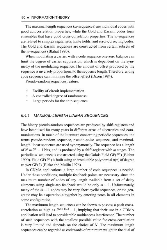
80 • INFORMATION THEORY
The maximal length sequences (m-sequences) are individual codes withgood autocorrelation properties, while the Gold and Kasami codes formensembles that have good cross-correlation properties. The m-sequencesare related to simplex signal sets, finite fields, and error-correcting codes.The Gold and Kasami sequences are constructed from certain subsets ofthe m-sequences (Blahut 1990).
When modulating a carrier with a code sequence one-zero balance canlimit the degree of carrier suppression, which is dependent on the sym-metry of the modulating sequence. The amount of offset produced by thesequence is inversely proportional to the sequence length.Therefore, a longcode sequence can minimize the offset effect (Dixon 1984).
Pseudo-random sequences feature:
• Facility of circuit implementation.• A controlled degree of randomness.• Large periods for the chip sequence.
6.4.1 MAXIMAL-LENGTH LINEAR SEQUENCES
The binary pseudo-random sequences are produced by shift-registers andhave been used for many years in different areas of electronics and com-munications. In much of the literature concerning periodic sequences, theterms pseudo-random sequence, pseudo-noise sequence, and maximal-length linear sequence are used synonymously. The sequence has a lengthof N = 2m − 1 bits, and is produced by a shift-register with m stages. Theperiodic m-sequence is constructed using the Galois Field GF(2m) (Blahut1990). Field GF(2m) is built using an irreducible polynomial p(x) of degreem over GF(2) (Blake and Mullin 1976).
In CDMA applications, a large number of code sequences is needed.Under these conditions, multiple feedback points are necessary since themaximum number of codes of any length available from a set of delayelements using single-tap feedback would be only m− 1. Unfortunately,many of the m− 1 codes may be very short cyclic sequences, or the gen-erator may halt operation altogether by entering zeros in all elements insome configuration.
The maximum length sequences can be shown to possess a peak cross-correlation as high as 2(m+1)/2 − 1, implying that their use in a CDMAapplication will lead to considerable multiaccess interference. The numberof such sequences with the smallest possible value for cross-correlationis very limited and depends on the choice of N . The maximum lengthsequences can be regarded as codewords of minimum weight in the dual of

CODE DIVISION MULTIPLE ACCESS • 81
a Hamming code, generated by a primitive polynomial. The dual containsonly one codeword and all its cyclic shifts.
Using all the possible linear combinations of feedback taps for an m-stage register, there are [φ(2m − 1)]/m maximal sequences that can begenerated. The last expression represents an Euler totient function, that is,the number of positive integers that are relatively prime to and less than2m − 1.
Table 6.1 lists the number of maximal sequences available for registerlengths 3 through 20. Among the listed sequences are also some Mersenneprime codes that are defined as those codes for which the code lengthN = 2m − 1 is a prime number (Dixon 1984). What is interesting aboutthe data presented in the table is the number of codes available, that isnot a monotonic function of the register length. For instance, it is alwayspreferable to use the least prime number for m as one progresses in thetable because it gives the maximum number of sequences.
When several users share the same channel without phase coherence,as in the case of a totally asynchronous system, it is desirable that thecross-correlation functions be small in absolute value. In addition, the
Table 6.1. Number of maximal sequences
m Number of codes Prime factors of 2m − 1
3 2 74 4 3 and 55 6 316 4 3, 3, and 77 18 1278 16 3, 5, and 179 48 7 and 7310 60 3, 11, and 3111 176 23 and 8912 96 3, 3, 5, 7, and 1313 630 8,19114 756 3, 43, and 12715 1,800 7, 31, and 15116 2,048 3, 5, 17, and 25717 7,710 131,07118 1,728 3, 3, 3, 7, 19, and 7319 27,594 524,28720 19,200 7, 7, 127, and 137

82 • INFORMATION THEORY
1 2 ... m-1 m
+
Figure 6.6. Pseudo-noise sequence generator
autocorrelation function must attain the maximum possible value. In matchedfilter detection, the output of the detector is the correlation of the input anda replica of the desired signal.
The investigation of lower bounds for the cross-correlation betweenpseudo-sequences is still a matter of research. One of the important resultsfor the multichannel case is due to Welch, and states that the lower boundon the peak magnitude of the cross-correlation rMAX is (Welch 1974)
rMAX ≥N
√M − 1
MN − 1(6.6)
in which the set is composed of M sequences of length N .
Example: for large values of N and M the bound is well approximatedas√
N .
6.4.2 GOLD SEQUENCES
A method for choosing the linear maximal codes, to be used as compo-nents of Gold sequences, was introduced in 1967 (Gold 1967). The Goldsequences are generated by modulo-2 addition of a pair of maximal-lengthsequences, as shown in Figure 6.7. The code sequences are added on achip basis, by synchronous clocking. The main feature of this type ofsequence generator is the large number of codes it supplies, although itrequires only one pair of feedback tap sets (Dixon 1984).
The Gold sequences are constructed from m-sequences. For a given mand a pair {a, b} of distinct m-sequences, the Gold code is the set
C={a, b, a+ T ib : i= 0, . . . , 2m − 2}. (6.7)
The Gold code contains 2m + 1 sequences of block-length 2m − 1. Theelements of the code are called Gold sequences. Sequences a and bare selected so their cross-correlation function has a maximum value

CODE DIVISION MULTIPLE ACCESS • 83
1 2 ... m-1 m
+
1 2 ... m-1 m
+
+ +
Figure 6.7. Gold sequence generator.
2�(m+2)/2� + 1. Such a pair of sequences will always exist. The cross-correlation functions and, except of the main peak, the autocorrelationfunctions of a Gold code can only take values in the set {−1,−2�(m+2)/2� −1, 2�(m+2)/2� − 1}.
Hence the largest magnitude of any cross-correlation of pairs of sequencesfrom C is 2�(m+2)/2� + 1 (Blahut 1990).Table 6.2 compares the relative peakcross-correlations for the m-sequences and Gold sequences (Proakis 1989).It can be seen that the periodic cross-correlation function between the pairsof m-sequences has large peaks when compared to the Gold sequences ofthe same period.
Table 6.2. Relative peak cross-correlations of m-sequences, Goldsequences and Kasami sequences
m m-sequences Gold sequences Kasami sequences
3 0.71 0.71 –4 0.60 0.60 0.335 0.35 0.29 –6 0.36 0.27 0.147 0.32 0.13 –8 0.37 0.13 0.079 0.22 0.06 –
10 0.37 0.06 0.0311 0.14 0.03 –12 0.34 0.03 0.03
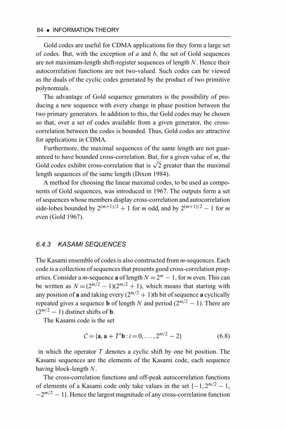
84 • INFORMATION THEORY
Gold codes are useful for CDMA applications for they form a large setof codes. But, with the exception of a and b, the set of Gold sequencesare not maximum-length shift-register sequences of length N . Hence theirautocorrelation functions are not two-valued. Such codes can be viewedas the duals of the cyclic codes generated by the product of two primitivepolynomials.
The advantage of Gold sequence generators is the possibility of pro-ducing a new sequence with every change in phase position between thetwo primary generators. In addition to this, the Gold codes may be chosenso that, over a set of codes available from a given generator, the cross-correlation between the codes is bounded. Thus, Gold codes are attractivefor applications in CDMA.
Furthermore, the maximal sequences of the same length are not guar-anteed to have bounded cross-correlation. But, for a given value of m, theGold codes exhibit cross-correlation that is
√2 greater than the maximal
length sequences of the same length (Dixon 1984).A method for choosing the linear maximal codes, to be used as compo-
nents of Gold sequences, was introduced in 1967. The outputs form a setof sequences whose members display cross-correlation and autocorrelationside-lobes bounded by 2(m+1)/2 + 1 for m odd, and by 2(m+1)/2 − 1 for meven (Gold 1967).
6.4.3 KASAMI SEQUENCES
The Kasami ensemble of codes is also constructed from m-sequences. Eachcode is a collection of sequences that presents good cross-correlation prop-erties. Consider a m-sequence a of length N = 2m − 1, for m even. This canbe written as N = (2m/2 − 1)(2m/2 + 1), which means that starting withany position of a and taking every (2m/2 + 1)th bit of sequence a cyclicallyrepeated gives a sequence b of length N and period (2m/2 − 1). There are(2m/2 − 1) distinct shifts of b.
The Kasami code is the set
C={a, a+ T ib : i= 0, . . . , 2m/2 − 2} (6.8)
in which the operator T denotes a cyclic shift by one bit position. TheKasami sequences are the elements of the Kasami code, each sequencehaving block-length N .
The cross-correlation functions and off-peak autocorrelation functionsof elements of a Kasami code only take values in the set {−1, 2m/2 − 1,−2m/2 − 1}. Hence the largest magnitude of any cross-correlation function

CODE DIVISION MULTIPLE ACCESS • 85
pairs of sequences from the code is 2m/2 + 1 (Blahut 1990). The Kasamisequences also satisfy the Welch bound, and are in this sense optimal(Proakis 1989).
It might be noted that if the sequences are allowed to be defined over thecomplex mth roots of unity, for some positive integer m, then the auto andcross-correlation properties of the sequences could be improved greatly,and still maintain the balanced and run properties of the m-sequences, thatis, there is approximately an even distribution of each of the 2m elementsof the Galois Field, and short runs of identical symbols are more likely toappear than longer runs (Komo and Liu 1990). An extensive work on thesubject of sequence design is found in (Sarwate and Pursley 1980).
Some attributes of spread spectrum, employed by CDMA systems, areimportant for personal communications systems, including the utilizationof the voice activity factor, no need for equalization, use of one radioper site, soft handoff, no need for guard time, sectorization for capacity,less fading for the wide-band signal, easy transition from current systems,capacity advantage, no frequency management or assignment needed, softcapacity, coexistence with other systems and suitability for microcell andin-building systems (Lee 1991).
Modeling a spread spectrum system implies the generation of randomsequences. Those sequences must exhibit the same properties, in order tobe eligible for CDMA use. In real life, practical constraints dictate the useof pseudo-random, or pseudo-noise sequences (PN), whose properties arewell-known.

CHAPTER 7
THE CAPACITY OF A CDMASYSTEM
7.1 INTRODUCTION
The area of Personal Communications Network (PCN) is a huge success inthe communications field. The main technology used in mobile communi-cations is code division multiple access (CDMA) that has some advantagesover the previous techniques. This chapter describes and analyzes a modelfor the discrete-input continuous-output, Direct-Sequence Spread Spec-trum (DSSS), Gaussian multiple access channel.
In this chapter, the modulation scheme is specialized, with the choiceof DPSK modulation. This modulation scheme deserves some comments.DPSK is regarded by many authors as a natural choice for CDMA, espe-cially if one considers a fading multipath environment, in which syn-chronous carrier recovery is a difficult task (Misser, Wijffels, and Prasad1991; Turin 1984b).
As a differentially coherent modulation technique, DPSK also compareswell to similar systems using coherent PSK modulation and is less trouble-some to demodulate in a complex environment such as an indoor wirelesschannel (Kavehrad and McLane 1985; Kavehrad and Ramamurthi 1987).The capacity of the PSK scheme, for the coding channel resulting fromhard decision detection, was computed in Sousa (1992). In this chapter,upper and lower bounds on the sum capacity are obtained and compared.
7.2 ANALYSIS OF A CDMA SYSTEM WITH A FIXEDNUMBER OF USERS AND SMALL SNR
One of the problems related to CDMA is the possibility of interferencewith existing systems (Kavehrad and McLane 1985). Unlike the former

88 • INFORMATION THEORY
techniques, CDMA has its capacity solely limited by the amount of inter-ference into the system, which allows any reduction in interference to beconverted directly and linearly into an increase in capacity (Gilhousen et al.1991).
The use of spread spectrum allows new users to share the spectrumwith existing ones. Because CDMA is interference limited, the numberof users that share the same spectrum, and still maintain an acceptableperformance, is determined by the interference generated by the set ofusers.
In CDMA systems, each user is given a distinct pseudo-random code,which either identifies the user to the central station in a star network, oraddresses another user in a more fully connected network (Turin 1984b).Hence, the users utilize the same bandwidth and therefore interfere, mak-ing a received signal appear noisier as the traffic increases in the system.The effect of the interfering energy depends on the processing gain of thespread spectrum technique.
As implied, spread spectrum systems are less subject to multipath signalvariations than conventional systems. In a direct sequence receiver, if thereflected signal is delayed compared to the direct signal by more than onecode chip, the reflected signal is treated as uncorrelated to the direct signal.
The higher the code chip rate, for a particular system, the smaller its mul-tipath problem. In the mobile environment, the result of multipath receptionis that a moving receiver is subject to rapid fading and peaking of its inputsignal as the direct and reflected signals cancel and reinforce each other.Stationary receivers are also subject to multipath, due to the reflecting andrefracting surfaces (Dixon 1984).
Researchers, industries, and prospective users of CDMA systems havebeen concerned with three major issues regarding the design of those sys-tems. The first one is the design of pseudo-noise sequences with goodautocorrelation and cross-correlation properties.
The second issue, is the evaluation of system performance, that can bedone in two ways: using the average probability of error or computing theoutage of the system.The probability of error is averaged over the ensembleof channels obtained from the assumed model.
In the case of time-varying channel and stationary terminal, outage indi-cates the fraction of time the terminal operates with an error probabilityabove the limit. For the time-invariant channel and mobile terminal, out-age indicates the fraction of building area where the terminal can operate(Kavehrad and Ramamurthi 1987).
The evaluation of the system capacity, or which transmission rate the sys-tem can support under given circumstances, is the third issue. The number

THE CAPACITY OF A CDMA SYSTEM • 89
of allocated users dictates the type of distribution to characterize the mul-tiple access interference.
A large number of subscribers favor the Gaussian approximation (Turin1984b) and, for many applications, this approximation is satisfactory evenfor a processing gain as low as N = 10 and moderate values of the signal tointerference ratio (Sousa 1990). On the other hand, the Gaussian approxi-mation is typically more accurate for smaller values of the SNR, or largemultiuser interference (Geraniotis and Ghaffari 1991).
For a small number of subscribers, considering that the MAI is additivelycomposed of cross-correlations limited to a few chips of coincidence, themaximum interference is too small to apply the central limit theorem (Brady1991), or the conditions for utilization of the theorem do not apply if certainparameters are held constant (Sadowsky and Bahr 1991).
But, even for a small number of users, accurate methods have beendevised to calculate multiple access error probabilities using the Gaussianapproximation (Holtzman 1992).This section is dedicated to the evaluationof the capacity of a CDMA system, when the number of users is heldconstant.
CDMA is a type of noncooperative channel, which has asynchronousmultiplexing, implying that the M information sources transmit througha common medium without any prearrangement among themselves. Thiskind of channel has been investigated for some time, in a general sense,and some interesting results were found (Sommer 1966; Verdú 1989b).
In this type of communications system, several users transmit simulta-neously and concurrently to a common receiver. Therefore, all componentsof the received signal are statistically independent and so, perform as inter-ference in respect to any other given signal.The CDMA channel is analyzedthrough the use of an information theoretic approach in this section.
The concept of capacity is used regarding the limitation in the transmis-sion rate due to bandwidth, or related aspects, while the idea of throughputis used when scheduling is the main concern in the performance evalua-tion of the system. In the case of CDMA, both factors are involved whichgives rise to the concept of sum capacity, or limiting throughput per unitbandwidth (Sousa 1989).
Because of the reasoning and considerations developed in the follow-ing, the term capacity, used heretofore, is equivalent to the concept of sumcapacity, derived in the cited article. The capacity is assumed for the caseof noncooperation among the users and each user contributes a small frac-tion of the traffic to the channel (Sousa 1989).
The CDMA noncooperative multiple access channel discussed in thissection has M binary inputs, Xi ∈Xi, and a single Gaussian output, Y ∈Y .

90 • INFORMATION THEORY
The output is the combination of the M inputs plus noise and can be assumedGaussian, using the central limit theorem for a large number of users(Sousa 1989).The channel is assumed memoryless and, for the assumptionsmade, the optimum receiver for a particular signal will be the maximumlikelihood receiver.
In the following, one considers the performance analysis of an asyn-chronous CDMA system using direct-sequence codes. Let bij =±1, i=0, 1, . . . , M , j=−∞, . . . ,∞ be a binary bit string that modulates theith transmitter and let the codes ci(t), i= 1, . . . , M , 0≤ t≤Tb form a setof quasi-orthogonal sequences, with cross-correlation given by
rij(τ )=∫ Tb
0ci(t)cj(t − τ ) dt, |τ | ≤Tb, i �= j (7.1)
which is uniformly small compared to their individual energy (Turin 1984b)
Ec=∫ Tb
0c2
i (t) dt, i= 1, . . . , M . (7.2)
At the reception side, the desired signal is represented by
xi(t)=∞∑
j=−∞bi�j/N�ci(t − jTb)φj(t) (7.3)
in which {φj(t)} is a set of orthonormal functions and [j/N ] represents thegreatest integer less than or equal to j/N . If modulation is used, along withrectangular chip pulses, the functions are given by
φj(t)= cos [ωc(t − jTb)]. (7.4)
Therefore, the signal whose reception is sought can be expressed as
xi(t)=∞∑
j=−∞bi�j/N�ci(t − jTb) cos [ωc(t − jTb)]. (7.5)
However, the M transmitted signals combine additively, giving for anyreceiver a total signal y(t), such that
y(t)=M∑
i=1
xi(t)+ n(t) (7.6)
in which n(t) is a zero mean Gaussian noise of double-sided power densityN0/2. Consequently, part of the total signal is viewed as noise for each
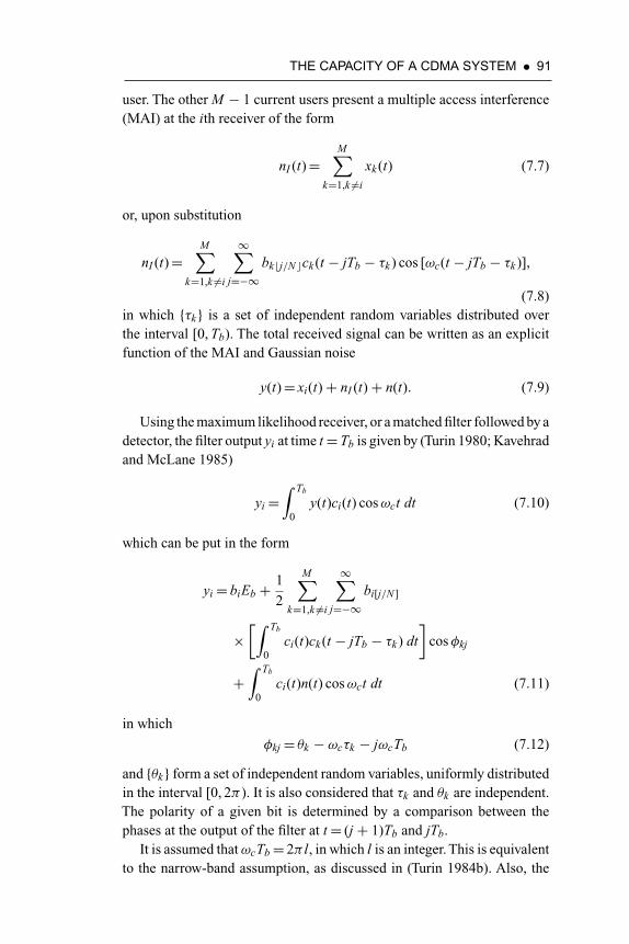
THE CAPACITY OF A CDMA SYSTEM • 91
user. The other M − 1 current users present a multiple access interference(MAI) at the ith receiver of the form
nI (t)=M∑
k=1,k �=i
xk (t) (7.7)
or, upon substitution
nI (t)=M∑
k=1,k �=i
∞∑j=−∞
bk�j/N�ck (t − jTb − τk ) cos [ωc(t − jTb − τk )],
(7.8)in which {τk} is a set of independent random variables distributed overthe interval [0, Tb). The total received signal can be written as an explicitfunction of the MAI and Gaussian noise
y(t)= xi(t)+ nI (t)+ n(t). (7.9)
Using the maximum likelihood receiver, or a matched filter followed by adetector, the filter output yi at time t=Tb is given by (Turin 1980; Kavehradand McLane 1985)
yi=∫ Tb
0y(t)ci(t) cos ωct dt (7.10)
which can be put in the form
yi= biEb + 1
2
M∑k=1,k �=i
∞∑j=−∞
bi[j/N ]
×[∫ Tb
0ci(t)ck (t − jTb − τk ) dt
]cos φkj
+∫ Tb
0ci(t)n(t) cos ωct dt (7.11)
in which
φkj = θk − ωcτk − jωcTb (7.12)
and {θk} form a set of independent random variables, uniformly distributedin the interval [0, 2π ). It is also considered that τk and θk are independent.The polarity of a given bit is determined by a comparison between thephases at the output of the filter at t= (j + 1)Tb and jTb.
It is assumed that ωcTb= 2π l, in which l is an integer. This is equivalentto the narrow-band assumption, as discussed in (Turin 1984b). Also, the
92 • INFORMATION THEORY
mean and variance of the third term are 0 and N0Eb/2, respectively, in which
Eb=∫ Tb
0c2
i (t) cos2 ωct dt, i= 1, . . . , M . (7.13)
The second term deserves some attention. It can be written as (Turin1984a)
Ni= 1
2
M∑k=1,k �=i
nk cos φkj (7.14)
in which
nk =∞∑
j=−∞bi[j/N ]
∫ Tb
0ci(t)ck (t − jTb − τk ) dt. (7.15)
But, the variance of the term nk , defined as σ 2k , inside the summation
can be expressed as
σ 2k = 2
∫ Tb/N
0
(1− Nτ
Tb
)2
(Tb − τ )dτ = 2
[T 2
b
3N− T 2
b
12N 2
]. (7.16)
Therefore, the variance of Ni, defined as σ 2i , is
σ 2i =
M − 1
8σ 2
k =(M − 1)T 2
b
12N− (M − 1)T 2
b
48N 2 . (7.17)
Because the MAI term is assumed Gaussian, and Eb=Tb/2, the fil-ter output is a Gaussian variable, with mean μI = biEb. Therefore, themultiple access variance σ 2
I is given by (Borth and Pursley 1979; Turin1984b; Pickholtz, Schilling, and Milstein 1982)
σ 2I =
(M − 1)E2b
3N− (M − 1)E2
b
12N 2 + N0Eb
2. (7.18)
Based on the results stated by Shannon (1948), the mutual informationbetween the ith individual input and the output, for the noncooperativeadditive channel, can be written as
I (Xi; Y )=H (Y )− H (Y − Xi)
=q−1∑j=0
∫ ∞−∞
p(y|xj)P(xj) logp(y|xj)
p(y)dy (7.19)
in which
p(y)=q−1∑j=0
p(y|xj)P(xj), (7.20)
the logarithms are to the base 2, unless otherwise stated, implying thatinformation rates are given in bits and q represents the number of signallevels.

THE CAPACITY OF A CDMA SYSTEM • 93
The maximization of Equation 7.19, over the set of input probabilities,gives the expressions for the individual capacities
Ci=maxP(xj)
q−1∑j=0
∫ ∞−∞
p(y|xj)P(xj) logp(y|xj)
p(y)dy. (7.21)
The expression is set as the maximum of the average mutual informationbetween the input X ={x1, . . . , xq−1} and the output Y = (−∞,∞).
For possible inputs xk =+1 and xk =−1, the average mutual informa-tion is maximized when the input probabilities are P(xk =+1)=P(xk =−1)= 1/2. Hence, the expression can be put in the form (Alencar andBlake 1993c)
Ci= 1
2
∫ ∞−∞
p(y| + Eb) logp(y| + Eb)
p(y)dy
+ 1
2
∫ ∞−∞
p(y| − Eb) logp(y| − Eb)
p(y)dy (7.22)
in which, assuming that nI (t) is Gaussian,
p(y| ± Eb)= 1
σI√
2πe− (y∓Eb)2
2σ2I . (7.23)
The noise variance σ 2I was obtained assuming that the interuser inter-
ference amounts to a Gaussian distribution, for a CDMA system usingdirect-sequence codes (Turin 1984b). It can be simplified by noting that forcik (t)=±1, k = 1, . . . , N , the code energy is Ec=Tb= 2Eb, and for usualvalues of the processing gain (Pursley 1977; Geraniotis and Pursley 1985)
σ 2I =
(M − 1)E2b
3N+ N0Eb
2(7.24)
in which M is the number of users in the channel, N is the processing gain,N0/2 is the Gaussian noise power spectrum density, and Tb is the bit time.
It can reasonably be argued, for the present model, that the sum capacityis a one-feature function containing most of the needed information aboutthe behavior of the system. This is fair to say for spread spectrum tech-niques, which define a noncooperative type of channel whose capacity isgiven by the sum of the individual capacities,
C=M∑
i=1
Ci. (7.25)

94 • INFORMATION THEORY
The individual rates, upon substitution of the appropriate terms, areequal to
Ci = 1
2σI
√2π
∫ ∞−∞
e− (y−Eb )2
2σ2I log
⎡⎣ 2 exp (− (y−Eb)2
2σ 2I
)
exp (− (y−Eb)2
2σ 2I
)+ exp (− (y+Eb)2
2σ 2I
)
⎤⎦ dy
+ 1
2σI
√2π
∫ ∞−∞
e− (y+Eb )2
2σ2I log
⎡⎣ 2 exp (− (y+Eb)2
2σ 2I
)
exp (− (y−Eb)2
2σ 2I
)+ exp (− (y+Eb)2
2σ 2I
)
⎤⎦ dy
which can be simplified to
Ci= 1
σI√
2π
∫ ∞−∞
e− (y−Eb)2
2σ2I log
⎡⎣ 2
1+ exp (− 2yEb
σ 2I
)
⎤⎦ dy. (7.26)
The remaining part of this section is concerned with establishing asuitable approximation for the sum capacity in Equation 7.26, in termsof upper and lower bounds, for small values of the signal to total noiseratio. Expanding the logarithm term in a power series in Eb, for low valuesof the signal-to-noise ratio (SNR), one obtains (Gallager 1968; Gradshteynand Ryzhik 1990)
log
⎡⎣ 2
1+ exp (− 2yEb
σ 2I
)
⎤⎦= log e
[yEb
σ 2I
− y2E2b
2σ 4I
+ y4E4b
12σ 8I
+ O(E6b )
].
(7.27)
The expansion is valid for the case in which the number of users in thesystem is much larger than the code length, or when the thermal noise ispreponderant in the system, according to Equation 7.13.
Substituting into Equation 7.26 and integrating, gives
Ci= log e
[E2
b
2σ 2I
− E4b
4σ 4I
+ E6b
2σ 6I
+ E8b
12σ 8I
+ O
(E10
b
σ 10I
)](7.28)
in which the remaining terms become insignificant as the SNR goes tozero. It is appropriate to say that spread spectrum systems operate, insome cases, under conditions of very low SNR. Therefore, neglectingall but the first term, one obtains an upper bound on the individualcapacity
Ci ≤ log e
[E2
b
σ 2I
](7.29)
THE CAPACITY OF A CDMA SYSTEM • 95
Because the series in 7.27 is an alternating one, a lower bound can befound easily considering also the second term
Ci ≥ log e
[E2
b
2σ 2I
− E4b
2σ 4I
]. (7.30)
Using the first term in Equation 7.27 as an approximation for the indi-vidual capacity and substituting the formula for the MAI variance one findsa formula for the capacity, under the assumption of very low SNR
Ci≈ log e
⎡⎢⎣ E2
b
2(
(M−1)E2b
3N + N0Eb2
)⎤⎥⎦ . (7.31)
Using now Equation 5.34, maximized for the case in which all the trans-mitters carry the same power, one obtains
C=MCi≈ 3 log eMN
2(M − 1)+ 3N N0Eb
. (7.32)
Example: interesting results are obtained when one varies the SNR Eb/N0
or number of users in the system. One gets, as the SNR goes to zero
limEbN0→0
C= 0 (7.33)
If the SNR is small, as compared to the ratio of processing gain to num-ber of users, Eb/N0� 3N/2(M − 1), then the capacity can be approxi-mated by
C≈ log eMEb
N0(7.34)
and the capacity is proportional to the SNR, as well as to the number ofchannel users.
Example: another interesting result can be obtained by taking the limit ofthe capacity when the number of sources goes to infinity, for a rectangularchip pulse,
limM→∞C≈ 3 log eN
2(7.35)

96 • INFORMATION THEORY
It is easy to conclude that, as the number of users increases towardsinfinity, the capacity region shrinks, and the channel capacity converges toa value that is proportional to the processing gain. In this case, by using aset of orthogonal spreading codes, the capacity becomes independent of theSNR and it is not possible to increase the capacity of the noncooperativechannel by increasing the power of the transmitted signals.
Because the limiting capacity C becomes dependent on the processinggain, as the number of senders goes to infinity, the only possibility left toboost the capacity is by an increase in the available bandwidth.This is one ofthe reasons why spread spectrum techniques are useful for noncooperativetype of systems. Figure 7.1 shows the relation between the exact (middlecurve) and the approximate capacity (upper and lower bounds) in termsof the SNR, for a given code length (N = 100) and a number of users(M = 500).
The exact formula is obtained from 7.26, after substitution into 5.34.The approximate value 7.32 is used as the upper bound. It is possible tonote that the upper and lower approximations are fairly close to the exactresult, if the SNR is below −5 dB.
C
Eb/No, dB
0-5-10-15-20
160
140
120
100
80
60
40
20
Capacity, bits per channel use
Upper boundLower bound
Figure 7.1. Capacity approximations for the channel, as a function of theSNR, for M = 500 and N = 100.
THE CAPACITY OF A CDMA SYSTEM • 97
7.3 CDMA SYSTEM WITH A FIXED NUMBER OFUSERS AND HIGH SNR
In the previous section, an approximation for the capacity of a CDMAsystem was obtained considering a small SNR. In that case, either thenumber of users was very large, as compared to the processing gain, or thesignal power was completely embedded in the Gaussian noise. This sectionpresents a set of approximations for the channel capacity, considering nowa large SNR, or a large ratio of processing gain to number of users.
In order to analyze the sum capacity in detail, it is important to findboth approximations and bounds for the function. The equation for theindividual capacity 7.26 can be simplified by the application of logarithmproperties to
Ci= 1
σI√
2π
∫ ∞−∞
e− (y−Eb)2
2σ2I
[1− log
(1+ exp (− 2yEb
σ 2I
)
)]dy (7.36)
which, upon integration of the first term, gives
Ci= 1− 1
σI√
2π
∫ ∞−∞
e− (y−Eb)2
2σ2I log
(1+ e
− 2yEbσ2
I
)dy. (7.37)
Expanding the exponent leads finally to
Ci= 1− log ee− E2
b2σ2
I1
σI√
2π
∫ ∞−∞
e− y2
2σ2I e− yEb
σ2I ln
(1+ e
− 2yEbσ2
I
)dy.
(7.38)
As seen from the analysis undergone in the last section, the integrand inthe above equation is suitable for a series expansion, as long asEb/N0� 1. In order to adjust the integrand, so that the expansion can holdfor Eb/N0� 1 as well, one can resort to the Fourier transform properties.The functions inside the integral
g(y)= 1
σI√
2πe− y2
2σ2I (7.39)
and
f (y)= e− yEb
σ2I ln
(1+ e
− 2yEbσ2
I
)(7.40)
can be Fourier transformed to (Gradshteyn and Ryzhik 1990),
G(ω)=F[g(y)]= e−σ2
N ω2
2 (7.41)
98 • INFORMATION THEORY
and
F(ω)=F[f (y)]=π csc
(π2 + jπσ 2
I ω
2Eb
)Eb
σ 2I+ jω
. (7.42)
Therefore, applying the Fourier transform property of the integral of theproduct of two functions,∫ ∞
−∞f (y)G(y)dy=
∫ ∞−∞
F(ω)g(ω) dω (7.43)
one obtains
Ci= 1− log e e− E2
b2σ2
I
∫ ∞−∞
e−σ2
I ω2
2
π csc(
π2 + jπσ 2
I ω
2Eb
)Eb
σ 2I+ jω
dω. (7.44)
This last integral can be simplified, using the following property ofhyperbolic functions
csc
(π
2+ jπσ 2
I ω
2Eb
)= sec
(jπσ 2
I ω
2Eb
)(7.45)
then
Ci= 1− log e e− E2
b2σ2
I
∫ ∞−∞
e−σ2
I ω2
2
π sec(
jπσ 2I ω
2Eb
)Eb
σ 2I+ jω
dω. (7.46)
The application of yet another simple property gives
Ci= 1− π log e e− E2
b2σ2
I
∫ ∞−∞
e−σ2
I ω2
2
cosh(
πσ 2I ω
2Eb
) (Eb
σ 2I+ jω
) dω. (7.47)
Multiplying and dividing the integrand by the conjugate of the complexterm in the denominator leads to
Ci= 1− π log e e− E2
b2σ2
I
∫ ∞−∞
e−σ2
I ω2
2
(Eb
σ 2I− jω
)cosh
(πσ 2
I ω
2Eb
) (E2
b
σ 4I+ ω2
) dω. (7.48)
The integral can now be split into two terms
Ci= 1− π log e e− E2
b2σ2
I
⎡⎢⎣∫ ∞−∞
e−σ2
I ω2
2
(Eb
σ 2I
)cosh
(πσ 2
I ω
2Eb
) (E2
b
σ 4I+ ω2
) dω
−∫ ∞−∞
jωe−σ2
I ω2
2
cosh(
πσ 2I ω
2Eb
) (E2
b
σ 4I+ ω2
) dω
⎤⎥⎦ . (7.49)

THE CAPACITY OF A CDMA SYSTEM • 99
But the second integrand is an odd function of ω and therefore integratesto zero. The first integrand is even, which yields finally
Ci= 1− 2π log e e− E2
b2σ2
IEb
σ 2I
∫ ∞0
e−σ2
I ω2
2
cosh(
πσ 2I ω
2Eb
) (E2
b
σ 4I+ ω2
) dω. (7.50)
The capacity can be lower and upper bounded by recognizing thatthe Cauchy function is upper bounded by 1 and lower bounded byexp (− σ 4
I ω2/E2b ), respectively. The lower bound is
Ci ≥ 1− 2π log e e− E2
b2σ2
Iσ 2
I
Eb
∫ ∞0
e−σ2
I ω2
2
cosh(
πσ 2I ω
2Eb
) dω (7.51)
and the upper bound
Ci ≤ 1− 2π log e e− E2
b2σ2
Iσ 2
I
Eb
∫ ∞0
e−σ2
I ω2
2
cosh(
πσ 2I ω
2Eb
)e− σ4
I ω2
E2b dω. (7.52)
Both expressions are good approximations for the actual value of thecapacity if Eb/σ
2I � 1, which implies N�M . For very long code sequences,
the hyperbolic cosine can also be simplified to
cosh
(πσ 2
I ω
2Eb
)= 1+ 1
2
(πσ 2
I ω
2Eb
)2
+ · · ·≈ 1 (7.53)
Using this simplification in Equation 7.51, one obtains the lower boundand approximation
Ci ≥ 1− 2π log e e− E2
b2σ2
Iσ 2
I
Eb
∫ ∞0
e−σ2
I ω2
2 dω. (7.54)
and finally
Ci ≥ 1− π3/2 log eσI
Ebe− E2
b2σ2
I . (7.55)
This exponential approximation, referred to as Bound 1, is plotted alongwith the exact capacity in Figure 7.2, for M = 20 and N = 100, after thesubstitution into the formula for the sum capacity.
On the other hand, another approximation can be attempted using Equa-tion 7.52, which can be put in the following form
Ci ≤ 1− 2π log e e− E2
b2σ2
Iσ 2
I
Eb
∫ ∞0
e−(
σ2I2 +
σ4I
E2b
)ω2
cosh(
πσ 2I ω
2Eb
) dω. (7.56)
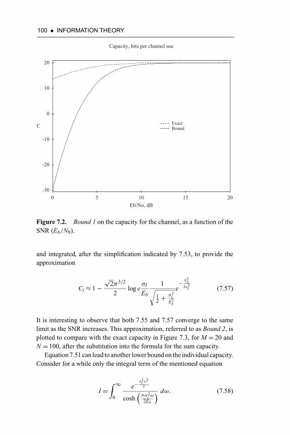
100 • INFORMATION THEORY
C
Eb/No, dB20151050
20
10
0
-10
-20
-30
Capacity, bits per channel use
ExactBound
Figure 7.2. Bound 1 on the capacity for the channel, as a function of theSNR (Eb/N0).
and integrated, after the simplification indicated by 7.53, to provide theapproximation
Ci≈ 1−√
2π3/2
2log e
σI
Eb
1√12 + σ 2
I
E2b
e− E2
b2σ2
I (7.57)
It is interesting to observe that both 7.55 and 7.57 converge to the samelimit as the SNR increases. This approximation, referred to as Bound 2, isplotted to compare with the exact capacity in Figure 7.3, for M = 20 andN = 100, after the substitution into the formula for the sum capacity.
Equation 7.51 can lead to another lower bound on the individual capacity.Consider for a while only the integral term of the mentioned equation
I =∫ ∞
0
e−σ2
I ω2
2
cosh(
πσ 2I ω
2Eb
) dω. (7.58)

THE CAPACITY OF A CDMA SYSTEM • 101
C
Eb/No, dB20151050
20
10
0
-10
-20
Capacity, bits per channel use
ExactBound
Figure 7.3. Bound 2 on the capacity for the channel, as a function of theSNR (Eb/N0).
It is not difficult to obtain a simpler expression, making use of the propertyof integration by parts,
I = 2Ebe−σ2
I ω2
2
πσ 2I
arctan
[sinh
(πσ 2
I ω
2Eb
)]∣∣∣∣∣∣∞
0
+∫ ∞
0
2Eb
πωe−
σ2I ω2
2 arctan
[sinh
(πσ 2
I ω
2Eb
)]dω. (7.59)
The first term on the right side of the expression vanishes, when the limitsare applied, yielding
I =∫ ∞
0
2Eb
πωe−
σ2I ω2
2 arctan
[sinh
(πσ 2
I ω
2Eb
)]dω. (7.60)
Using the usual assumption Eb/σ2I � 1, and the inequality arctan (x)≤ x
it is possible to upper bound the integrand, obtaining
I ≤ 2Eb
π
∫ ∞0
ωe−σ2
I ω2
2 sinh
(πσ 2
I ω
2Eb
)dω. (7.61)

102 • INFORMATION THEORY
which integrates to (Gradshteyn and Ryzhik 1990)
I ≤√
2π
2σ 2I
eπ2σ2
I8E2
b . (7.62)
Substituting the above equation into Equation 7.51 gives
Ci ≥ 1−√2π3/2 log eσI
Ebe− E2
b2σ2
I+ π2σ2
I8E2
b . (7.63)
The final version of the bound is found introducing the expression forthe multiple access interference plus noise
σ 2I =
(M − 1)E2b
3N+ N0Eb
2(7.64)
into Equation 7.63. This yields
Ci ≥ 1−√2π3/2 log e
√M − 1
3N+ N0
2Eb
× exp
[− 3N
2(M − 1)+ 3N N0Eb
+ π2
8
(M − 1
3N+ N0
2Eb
)](7.65)
and the total capacity, or sum capacity, is lower bounded by
C≥M −√2π3/2 log eM
√M − 1
3N+ N0
2Eb
× exp
[− 3N
2(M − 1)+ 3N N0Eb
+ π2
8
(M − 1
3N+ N0
2Eb
)](7.66)
which is depicted, as a function of the SNR, in Figure 7.4 and referred toas Bound 3, for M = 20 and N = 100.
Example: two cases of interest are obtained by making Eb/N0→∞
C≥M −√2π3/2 log eM
√M − 1
3Nexp[− 3N
2(M − 1)+ π2
24
M − 1
N
](7.67)
and N→∞
C≥M −√2π3/2 log eM
√N0
2Ebexp[−Eb
N0+ π2
16
N0
Eb
](7.68)

THE CAPACITY OF A CDMA SYSTEM • 103
C
Eb/No, dB20151050
20
0
-20
-40
-60
-80
-100
-120
Capacity, bits per channel use
ExactBound
Figure 7.4. Bound 3 on the capacity for the channel, as a function of theSNR (Eb/N0).
The bound for the sum capacity can be expressed in terms of the prob-ability of error, using Equation 7.82
C≥M − 2π3/2 log ePeM
√1
ln (1/2Pe)exp(
π2
8
1
2 ln (1/Pe)
)(7.69)
7.4 A TIGHT BOUND ON THE CAPACITY OF ACDMA SYSTEM
In this section a lower bound on the sum capacity, for a CDMA system,is obtained. The bound is shown to be very tight, although not an expo-nential one, and therefore amenable for computation in place of the actualformula for the system capacity, which involves a time consuming numer-ical integration. Some results are reported in this section, in terms of theprocessing gain, number of users and SNR. An interesting threshold is dis-covered, relating the sequence length, or processing gain, and the numberof users in the channel. Conditions for attaining the capacity are establishedand the capacity is plotted as a function of the probability of error.
104 • INFORMATION THEORY
The following derivation presents a lower bound for the channel capac-ity, considering a large SNR, or a large ratio of processing gain to numberof users. This is likely to be the case in real systems, because both assump-tions decrease the probability of error. In order to set the stage for theevaluation of the lower bound, it is interesting to present a slightly differentformulation from that one presented in the past section. One begins withEquation 7.47, repeated here for reference
Ci= 1− π log e e− E2
b2σ2
I
∫ ∞−∞
e−σ2
I ω2
2
cosh(
πσ 2I ω
2Eb
) (Eb
σ 2I+ jω
) dω. (7.70)
The integral inside Equation 7.50, in last section, is not amenable foran analytic solution. One form of attacking the problem is to find a boundfor the capacity, by a convenient substitution implied by the inequalitycosh (x)≥ 1+ x2
2 . Then,
Ci ≥ 1− 2π log e e− E2
b2σ2
IEb
σ 2I
∫ ∞0
e−σ2
I ω2
2[1+ 1
2
(πσ 2
I ω
2Eb
)2] (
E2b
σ 4I+ ω2
) dω.
(7.71)
Rearranging the equation, in order to come out with a standard definiteintegral, one obtains
Ci ≥ 1− 2π log e e− E2
b2σ2
I8E3
b
π2σ 6I
∫ ∞0
e−σ2
I ω2
2(8E2
b
π2σ 4I ω+ ω2
) (E2
b
σ 4I+ ω2
) dω
(7.72)which can be separated by a partial fraction expansion to
Ci ≥ 1− 2π log e e− E2
b2σ2
I8Eb
(π2 − 8)σ 2I
×⎡⎢⎣∫ ∞
0
e−σ2
I ω2
2(8E2
b
π2σ 4I ω+ ω2
)dω −∫ ∞
0
e−σ2
I ω2
2(E2
b
σ 4I+ ω2
) dω
⎤⎥⎦ .
The above integrals can then be evaluated by noting that (Gradshteynand Ryzhik 1990)∫ ∞
0
e−μ2x2
x2 + β2 dx= [1− erfc(βμ)]π
2βeβ2μ2
(7.73)
for Reβ > 0 and |argμ|< π/4.
THE CAPACITY OF A CDMA SYSTEM • 105
Therefore,
Ci ≥ 1− log e e− E2
b2σ2
I2π
π2 − 8
[[1− erf
(2Eb
πσI
)]
× π√2
e4E2
bπ2σ2
I −[
1− erf(
Eb√2σI
)]2e
E2b
2σ2I
⎤⎦ (7.74)
in which erf (x) is defined as
erf (x)= 2√π
∫ x
0e−t2
dt. (7.75)
This equation can be further simplified to
Ci ≥ 1− log e2π
π2 − 8
⎡⎣ π√
2
[1− erf
(2Eb
πσI
)]e
8−π2
2π2E2
bσ2
I
− 2[
1− erf(
Eb√2σI
)]]. (7.76)
Substituting now the expression for the total noise variance into Equa-tion 7.76 leads to the final expression for the lower bound on the sumcapacity
C≥M − log e2πM
π2 − 8(7.77)
×[
π√2
[1− erf
(2
π
√6NEb/N0
2(M − 1)Eb/N0 + 3N
)]
× e8−π2
2π26NEb/N0
2(M−1)Eb/N0+3N
− 2
[1− erf
(1√2
√6NEb/N0
2(M − 1)Eb/N0 + 3N
)]].
Equation 7.77 is plotted in Figure 7.5, along with the exact solution(upper curve), as a function of the SNR (SNR=Eb/N0, dB) for M = 20and sequence length N = 100. It is remarkable to notice that the differencedoes not exceed 5 percent from −10 dB to 20 dB and actually convergesto zero as the SNR increases. The lower bound will thus be used as anapproximation for the actual capacity in the following, for values of SNRof −10 dB or more.
One of the reasons for having a bound on the capacity, of the formexpressed by Equation 7.77, is the possibility of interpreting correctly therole of the many parameters on the performance of the system, because

106 • INFORMATION THEORY
C
Eb/No, dB02151050-5-10
20
18
16
14
12
10
8
6
4
2
Capacity, bits per channel use
ExactBound
Figure 7.5. Capacity for the channel, compared with the lower bound,as a function of the SNR (Eb/N0), for M = 20 and sequence lengthN = 100.
those parameters, and their relationship, appear explicitly in the formulafor the bound. As will be seen in what follows, some parameters have theproperty of influencing and even disrupting the system.
The second reason involves the possibility of combining different for-mulas, to attain a certain objective, as in the case of expressing the capacityas a direct function of the probability of error and vice-versa.
The third reason is related to computational resources. Evaluation ofthe exact solution is time and memory consuming and is justified onlywhen no feasible approximation is available. It is instructive to recall thateven in the case when the exact solution is being computed, the computersystem will always resort to some form of approximation or truncation ofthe formulas.
Equation 7.77 is also plotted in Figure 7.6, as a function of the SNR,for M = 20, having the sequence length as a parameter. It is interesting tonotice that for a high processing gain there is no further significant gain incapacity if N ≥ 10 M .
In Figure 7.7, the capacity is displayed as a function of the sequencelength, for a SNR of 10 dB, parametrized by the number of users. It must

THE CAPACITY OF A CDMA SYSTEM • 107
C
N=200
N=100
N=80
N=60
N=40
N=20
Eb/No, dB02151050-5-10
20
18
16
14
12
10
8
6
4
2
Capacity, bits per channel use
Figure 7.6. Approximate capacity for the channel, as a function of thesignal-to-noise ratio (Eb/N0), for M = 20, having N as a parameter.
be noticed that the capacity of the system is achieved for a sequence lengthof N = 100 and N = 200, for M = 10 and M = 20, respectively.
In Figure 7.8, the capacity is shown in terms of the number of users,for a given SNR (10 dB), and two values of the processing gain N = 100and N = 200 (upper curve). This result shows that the capacity for thebinary case, in bits per channel use, is numerically equal to the numberof users, as long as this number is small compared to the processing gain.Any increase in the number of users above M = 0.2N produces a transmis-sion rate that falls short of the system capacity. This is in agreement withprevious results (Turin 1984b; Pickholtz, Schilling, and Milstein 1982),contradicting (Hui 1984b), which suggested that using long PN sequenceswould decrease the sum capacity. Figure 7.9 illustrates the previous point,by showing a decrease in the capacity with an increase in the number ofusers, for a fixed value of N . It is important to mention that if both M andN increase to infinity, the limiting capacity will be given by log e/2, aspredicted in Chapter 2 (Sousa 1989).
The importance of finding a lower bound on the capacity is due to thenature of the noncooperativeness of CDMA. In this case, the lower bound

108 • INFORMATION THEORY
C
M=100
M=80
M=60
M=40
M=20
M=10
N
20018016014012010080604020
0
80
60
40
20
Capacity, bits per channel use
Figure 7.7. Capacity for the channel, using the approximate formula, asa function of the sequence length (N ), for different values of M .
represents the worst possible scenario for the system, which is incidentallyclose to reality.
Example: from Equation 7.77 it is also possible to draw some limitingresults, which are supposed to hold for the exact formula for the capacity.If the processing gain increases to infinity
limN→∞C=M . (7.78)
In case the SNR goes to infinity
limEbN0→∞
C=M . (7.79)
Finally, if the number of users increases without bound the sum capacitydisplays a peculiar behavior. If M ≥ 36N
limM→∞C= 0 (7.80)
otherwiselim
M→∞C=∞. (7.81)

THE CAPACITY OF A CDMA SYSTEM • 109
M
C
200180160140120100806040200
160
140
120
100
80
60
40
20
0
Capacity, bits per channel use
N=200N=100
Figure 7.8. Capacity for the channel, as a function of the number of users(M ), using the approximation for the capacity.
The relation between the number of users and the sequence length,χ =M/N , has been explored in a recent paper (Sousa 1989). It is remark-able that χ = 36 sets a threshold for the capacity, as the number of usersincreases to infinity. This channel behavior demands further study. It israther interesting to observe that the capacity can be achieved, for M→∞,as long as the sequence length increases accordingly.
It is useful to express the sum capacity in terms of the error probabil-ity. A complete analysis of a DSSS with DPSK modulation, in terms ofprobability of error, can be found in Kavehrad and Ramamurthi (1987) orin Geraniotis and Pursley (1986). In the following, a simplified analysis ispursued. This can be done, by rewriting the formula for the probability oferror for the DPSK system, considering now the effect of multiple accessinterference (Turin 1984b).
Pe= 1
2exp
[−1
2
(M − 1
3N+ N0
2Eb
)−1]
(7.82)
solving the expression for Eb/N0
ln 2Pe=−1
2
(M − 1
3N+ N0
2Eb
)−1
(7.83)
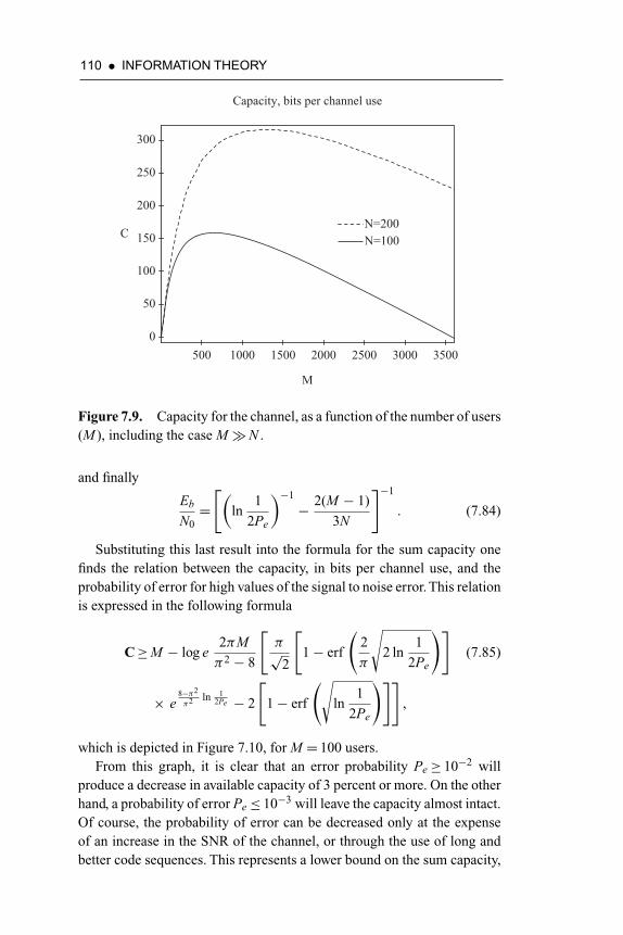
110 • INFORMATION THEORY
M
350030002500200015001000500
C
300
250
200
150
100
50
0
Capacity, bits per channel use
N=100N=200
Figure 7.9. Capacity for the channel, as a function of the number of users(M ), including the case M�N .
and finally
Eb
N0=[(
ln1
2Pe
)−1
− 2(M − 1)
3N
]−1
. (7.84)
Substituting this last result into the formula for the sum capacity onefinds the relation between the capacity, in bits per channel use, and theprobability of error for high values of the signal to noise error. This relationis expressed in the following formula
C≥M − log e2πM
π2 − 8
[π√
2
[1− erf
(2
π
√2 ln
1
2Pe
)](7.85)
× e8−π2
π2 ln 12Pe − 2
[1− erf
(√ln
1
2Pe
)]],
which is depicted in Figure 7.10, for M = 100 users.From this graph, it is clear that an error probability Pe ≥ 10−2 will
produce a decrease in available capacity of 3 percent or more. On the otherhand, a probability of error Pe ≤ 10−3 will leave the capacity almost intact.Of course, the probability of error can be decreased only at the expenseof an increase in the SNR of the channel, or through the use of long andbetter code sequences. This represents a lower bound on the sum capacity,

THE CAPACITY OF A CDMA SYSTEM • 111
Pe
C
0.010.0080.0060.0040.002
100
99.5
99
98.5
98
97.5
Capacity, bits per channel use
Figure 7.10. Capacity for the channel, as a function of the probability oferror (Pe).
for a given probability of error, which also implies the worst case for thesystem operation.
In order to conclude this section, it is useful to express Equation 7.77 in amore simplified form, as an exponential bound, to sum up the results fromthe previous section. It is not difficult to recognize in Equation 7.77 thecomplementary error function, erfc(x)= 1− erf (x), which can be approx-imated by (Schwartz 1970)
erfc(x)≈ e−x2
x√
π, x� 1. (7.86)
Therefore, after the appropriate substitution, one finds the exponentialapproximation below
Ci≈ 1−√
2π
2log e
σI
Ebe− E2
b2σ2
I . (7.87)
This formula will be referred to as Bound 4 in the following. It is plottedin Figure 7.11 for M = 20 users and gain N = 100.
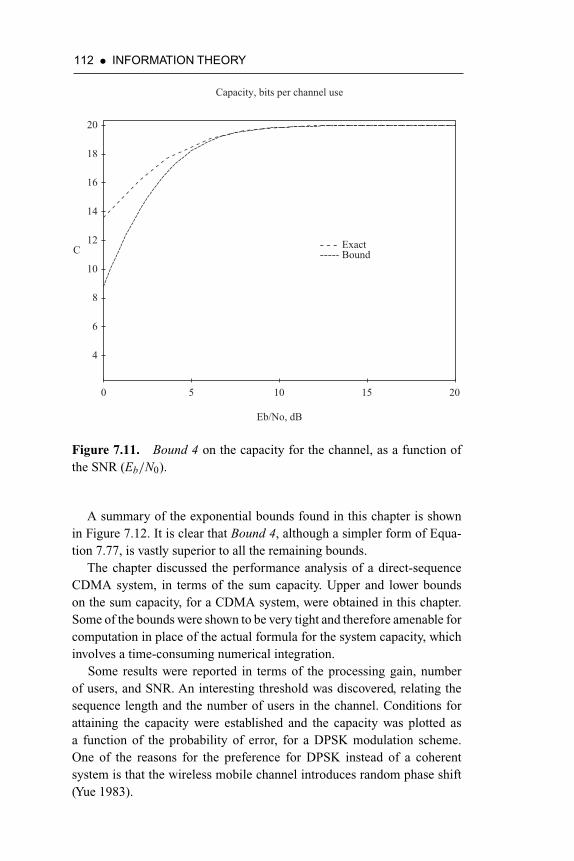
112 • INFORMATION THEORY
C
Eb/No, dB
20151050
20
18
16
14
12
10
8
6
4
Capacity, bits per channel use
ExactBound
Figure 7.11. Bound 4 on the capacity for the channel, as a function ofthe SNR (Eb/N0).
A summary of the exponential bounds found in this chapter is shownin Figure 7.12. It is clear that Bound 4, although a simpler form of Equa-tion 7.77, is vastly superior to all the remaining bounds.
The chapter discussed the performance analysis of a direct-sequenceCDMA system, in terms of the sum capacity. Upper and lower boundson the sum capacity, for a CDMA system, were obtained in this chapter.Some of the bounds were shown to be very tight and therefore amenable forcomputation in place of the actual formula for the system capacity, whichinvolves a time-consuming numerical integration.
Some results were reported in terms of the processing gain, numberof users, and SNR. An interesting threshold was discovered, relating thesequence length and the number of users in the channel. Conditions forattaining the capacity were established and the capacity was plotted asa function of the probability of error, for a DPSK modulation scheme.One of the reasons for the preference for DPSK instead of a coherentsystem is that the wireless mobile channel introduces random phase shift(Yue 1983).

THE CAPACITY OF A CDMA SYSTEM • 113
C
a
bc
de
a: Exactb: Bound 4c: Bound 2d: Bound 1e: Bound 3
Eb/No, dB0 2015105
20
0
-20
-40
-60
-80
-100
-120
Capacity, bits per channel use
Figure 7.12. Bounds on the capacity, as a function of the SNR (Eb/N0).
It is instructive to compare the new bound in Equation 7.77 with existingbounds and approximations on the sum capacity and with the exact solution.This is done in Figure 7.13, in which the upper curve (solid line) is the exactsolution and the previous bounds are given below, for M = 20 users andN = 100
C≈−M log(
1
2+ 1
2e−Eb/σI
), (7.88)
C≥ M
2log(
1+ Eb
σI
)− M
2log(
1+ Eb
5σI
)− M
2log(
5πe
24
)(7.89)
and
C≥M −Me−3Eb/4σI
(3πEb
4σI
)−1/2
−Mh
(e−3Eb/4σI
(3πEb
4σI
)−1/2)
, (7.90)

114 • INFORMATION THEORY
C
Eb/No, dB302520151050
1
.8
.6
.4
.2
Capacity, bits per channel use
Numerical SolutionEquation 11Equation 12Equation 13Equation 14
Figure 7.13. Comparison between the new and existing bounds, as afunction of the SNR (Eb/N0), for M = 20 and N = 100.
in which σI is given by Equation 7.24. Equation 7.13 is the correctedversion of the bound given by Shamai, Ozarow, and Wyner (1991) andh(x)=−x log x − (1− x) log (1− x) is the binary entropy function (Ozarowand Wyner 1990).
Substitution of the appropriate parameters and simplification of theresulting expressions yields
C≈−M log(
1
2+ 1
2e−√
6NEb/N02(M−1)Eb/N0+3N
), (7.91)
C≥ M
2log
[1+
√6NEb/N0
2(M − 1)Eb/N0 + 3N
]
− M
2log
[1+ 1
5
√6NEb/N0
2(M − 1)Eb/N0 + 3N
]
− M
2log(
5πe
24
)(7.92)
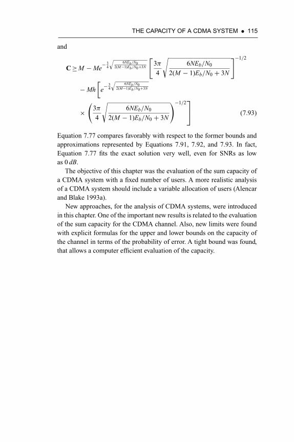
THE CAPACITY OF A CDMA SYSTEM • 115
and
C≥M −Me− 3
4
√6NEb/N0
2(M−1)Eb/N0+3N
[3π
4
√6NEb/N0
2(M − 1)Eb/N0 + 3N
]−1/2
−Mh
[e− 3
4
√6NEb/N0
2(M−1)Eb/N0+3N
×(
3π
4
√6NEb/N0
2(M − 1)Eb/N0 + 3N
)−1/2⎤⎦ (7.93)
Equation 7.77 compares favorably with respect to the former bounds andapproximations represented by Equations 7.91, 7.92, and 7.93. In fact,Equation 7.77 fits the exact solution very well, even for SNRs as lowas 0 dB.
The objective of this chapter was the evaluation of the sum capacity ofa CDMA system with a fixed number of users. A more realistic analysisof a CDMA system should include a variable allocation of users (Alencarand Blake 1993a).
New approaches, for the analysis of CDMA systems, were introducedin this chapter. One of the important new results is related to the evaluationof the sum capacity for the CDMA channel. Also, new limits were foundwith explicit formulas for the upper and lower bounds on the capacity ofthe channel in terms of the probability of error. A tight bound was found,that allows a computer efficient evaluation of the capacity.


CHAPTER 8
THEORETICAL CRYPTOGRAPHY
8.1 INTRODUCTION
Cryptography is the basis for network security. It comes from the Greekword kryptos, for tomb, hidden, or secret, combined with graphein, orwriting. A free translation is hidden writing, which defines the proposal ofcyphering a message. Cryptology, combines the same previous prefix withlogia, meaning study, to give the translation of study of secret coding.
Cryptography is the practice and study of techniques for secure commu-nication in the presence of third parties. It is also a collection of techniquesfor construction and analysis of protocols to overcome the influence of jam-mers and which are related to various aspects of information security, suchas data confidentiality, data integrity, authentication, and nonrepudiation.
Along the centuries, governments used cryptography to cypher mes-sages, supposed to remain in secrecy, while the spies tried to decipher them.During the wars, cryptography becomes more important, considering thenature of the operations.
Bletchley Park was the secret information and counter-information cen-ter in Great Britain during the Second World War. It was so secret that itremained as a legend after the end of the war, while England continuedto break the codes of other countries, either enemies or friends (Haykin1999).
The first computer, the Collossus, was built in Bletchley Park, devel-oped by Alan Mathison Turing (1912–1954), one of the greatest computergeniuses of the World. Destroyed after the end of the war, the Collosus wasrebuilt from the original drawings.
The German Enigma code was broken there with the help of Turing,who benefited from the information passed by a Hungarian mathematician

118 • INFORMATION THEORY
and a German officer, who provided information to French spies in ex-change for money. The French did not know how to decipher the code, andpassed on the information to the British.
8.2 CRYPTOGRAPHIC ASPECTS OF COMPUTERNETWORKS
The Internet has revolutionized the ways in which companies do business,since the Internet Protocol (IP) is undeniably efficient, inexpensive, andflexible. This section presents the main cryptographic aspects of modernTCP and IP computer networks, which include digital signature technol-ogy based on asymmetrical cryptographic algorithms, data confidentialityby applying symmetrical cryptographic systems, and system Public KeyInfrastructure (PKI) (Tanenbaum 2003).
The possible vulnerabilities of TCP and IP computer networks, andpossible techniques to eliminate them, are considered. It seem that only ageneral and multilayered security infrastructure could cope with possibleattacks to the computer network systems.
8.2.1 POTENTIAL VULNERABILITIES OF COMPUTERNETWORKS
The IP is efficient, inexpensive, and flexible. However, the existing meth-ods used to route IP packets leave them vulnerable to security risks, suchas spoofing, sniffing, and session hijacking, and provide no form of nonre-pudiation for contractual or monetary transactions.
Organizations need to secure communications between remote offices,business partners, customers, and travelling and telecommuting employees,besides securing the internal environment. The transmission of messagesover the Internet or intranet poses a risk, given the lack of protection at theexisting Internet backbone.
Control and management of security and access between the entitiesin a company’s business environment is important. Without security, bothpublic and private networks are susceptible to unauthorized monitoring andaccess. Internal attacks might be a result of minimal or nonexistent intranetsecurity.
Risks from outside the private network originate from connections tothe Internet and extranets. Password-based user access controls alone donot protect data transmitted across a network. Without security measuresand controls in place, the data might be subjected to attack. Some attacks

THEORETICAL CRYPTOGRAPHY • 119
Messagesource
Key generation
Encryption Decryption
Cryptanalysis
DestinationY
K
X X
Figure 8.1. General model for a cryptosystem.
are passive, and the information is only monitored. Other attacks are active,and the information is altered to corrupt or destroy the data or the networkitself.
8.3 PRINCIPLES OF CRYPTOGRAPHY
The general model for an encryption system is shown in Figure 8.1. Theoriginal message, also called plaintext and denoted by the letter X , is con-verted to an apparently random sequence called ciphertext and denoted bythe letter Y . The encryption process consists of an encipherment algorithmthat uses a key K , which is independent of the plaintext. The algorithmproduces a different output depending on the key used (Stallings 1999).
It is important to consider that a cryptanalyst, or hacker, could observethe encrypted message and try to decode it. The algorithm must, therefore,be powerful enough to resist the attack.
Encryption can be seen as a transformation, parametrized by K ,
Y =E(X , K), (8.1)
which converts the original text X to the ciphertext Y , to be transmitted.At the reception side, the inverse transformation is performed on the
ciphertext to produce the plaintext
X =D(Y , K). (8.2)
Of course, the destination must possess the key to be able to invert thetransformation. Therefore, the transmission of the key is an important partof the cryptobusiness.

120 • INFORMATION THEORY
The security of a cryptosystem depends on certain assumptions:
• The encryption algorithm must be robust enough that is difficult todecipher a message based only on the ciphertext.
• The key must be kept secret, and a secure channel should be pro-vided for transmission.
• There is no need to keep the algorithm secret.
The application of cryptographic techniques depends on the knowledgeof the security of the employed system. A cryptographic system can beclassified as:
1. How to transform the plaintext to the ciphertext, as the encryptionalgorithms are based on two principles (Stallings 1999):
a. Substitution, in which the individual symbols of the originaltext (bit, byte, letter, words) are mapped into other elements.
b. Transposition, in which the elements of the original text arerearranged.
2. How the original text is processed, which involves a block cipher,that processes a block of plaintext at a time, or a convolutionalcipher, also called stream cipher that processes the input symbolsas they arrive at the encryption subsystem.
3. How the key is generated, which can lead to the production ofa single, or symmetric, key to be used by both the transmitter andreceiver, or use different keys for the sender and receiver, also calledasymmetric or public key encryption.
8.4 INFORMATION THEORETICAL ASPECTS OFCRYPTOGRAPHY
It is possible to use the terminology of information theory to describe asecure encryption system. The measure of information, or entropy, of aplaintext, considered as a subset of symbols selected from the set of allpossible messages, is given by (van der Lubbe 1997)
H (X )=−L∑
l=1
p(xl) log p(xl), (8.3)
in which p(xl), l= 1, 2, . . . L represent the uncertainty of occurrence of thepossible plaintexts, considering that the texts are mutually independent.

THEORETICAL CRYPTOGRAPHY • 121
The entropy of the set of keys is given by
H (K)=−M∑
m=1
p(km) log p(km), (8.4)
in which km, m= 1, 2, . . . M are the possible keys.By the same token, it is possible to introduce a measure of information
for the ciphertext
H (Y )=−N∑
n=1
p(yn) log p(yn), (8.5)
in which p(yn), n= 1, 2, . . . N represent the uncertainty of occurrence of thepossible ciphertexts, considering that the texts are mutually independent.Usually, regarding the bijection from the plaintext into the ciphertext set,one considers N =L.
The conditional entropy, or key equivocation, is a measure of the uncer-tainty or information with respect to the key, when the ciphertext is availableis defined as
H (K |Y )=M∑
m=1
N∑n=1
p(km, yn) log p(km|ym). (8.6)
The uncertainty with respect to the plaintext, or conditional entropywhen the ciphertext is available, also known as message equivocation, isdefined as
H (X |Y )=L∑
l=1
N∑n=1
p(xl , yn) log p(xl |ym). (8.7)
The conditional entropy, or uncertainty with respect to the key, for agiven plaintext and corresponding ciphertext, is defined as
H (K |X , Y )=M∑
m=1
L∑l=1
N∑n=1
p(km, xl , yn) log p(km|xl , ym), (8.8)
which is also known as key appearance equivocation.Finally, the conditional entropy, or uncertainty with respect to the plain-
text, when the key and the ciphertext are known, is defined as
H (X |Y , K)=L∑
l=1
N∑n=1
M∑m=1
p(xm, yl , kn) log p(xm|yl , km). (8.9)
122 • INFORMATION THEORY
Since there is a bijection between the plaintext and ciphertext sets, it isalways true that
H (X |Y , K)= 0. (8.10)
As expected, when the ciphertext and the key are available it is possibleto retrieve the plaintext correctly, because the uncertainty with respect toX is null. There is no loss of information whatsoever at the receiver, andthe full original message is recovered.
8.4.1 RELATIONS BETWEEN THE ENTROPIES
A cipher system user requires that the key appearance equivocation, orH (K |X , Y ), be as high as possible, because if a cryptanalyst managesto obtain both the plaintext and the ciphertext, then the uncertainty withrespect to the key must be as large as possible.
This can be seen by the following argument. From the previous resultsin information theory, the joint measure of information in the plaintext,ciphertext, and key is
H (X , Y , K)=H (X |Y , K)+ H (Y , K)=H (K |X , Y )+ H (X , Y ). (8.11)
Also, consider the following relations
H (Y , K)=H (K |Y )+ H (Y ), (8.12)
and
H (X , Y )=H (X |Y )+ H (Y ). (8.13)
Combining the equations, one obtains
H (X |Y , K)+ H (K |Y )=H (K |X , Y )+ H (X |Y ). (8.14)
But, as discussed, H (X |Y , K)= 0, which results in
H (K |Y )=H (K |X , Y )+ H (X |Y ), (8.15)
which leads to
H (K |X , Y )=H (K |Y )− H (X |Y ). (8.16)
THEORETICAL CRYPTOGRAPHY • 123
Therefore, to obtain a large key appearance equivocation the messageequivocation H (X |Y ) must be small. However, a small message equivo-cation implies that the uncertainty with respect to the plaintext, when theciphertext is known, is small. But this is what must be avoided by thecryptosystem.
The uncertainty with respect to the key must be large to decrease theuncertainty with respect to the plaintext, and an increase in the uncertaintywith respect to the plaintext decreases the uncertainty with respect to thekey (van der Lubbe 1997).
8.5 MUTUAL INFORMATION FORCRYPTOSYSTEMS
The information theoretical approach provides additional results. Themutual information of the plaintext and the ciphertext is defined as
I (X ; Y )=H (X )− H (X |Y )=H (Y )− H (Y |X ). (8.17)
As expected, the objective of the cryptodesigner is to minimize themutual information I (X ; Y ). If the ciphertext provides no information aboutthe original message, then
H (X |Y )=H (X ),
and the mutual information between the plaintext and the encoded mes-sage is zero, or I (X ; Y )= 0. This is referred to as the absolutely securecryptosystem.
It is possible to obtain a lower limit for the mutual information betweenthe plaintext and the ciphertext. First, consider Equation 8.16, and sinceH (K |X , Y )≥ 0, it follows that
H (K |Y )≥H (X |Y ). (8.18)
The use of one of the properties of entropy gives
H (K)≥H (K |Y ), (8.19)
and therefore,H (K)≥H (X |Y ). (8.20)
Substituting this last inequality into Equation 8.17 gives
I (X ; Y )≥H (X )− H (K). (8.21)

124 • INFORMATION THEORY
Inequality 8.21 implies that a decrease in the uncertainty of a set ofkeys improves, on average, the independence between the plaintext and theciphertext.
It is implicit in the derivation that absolute security of a cryptosystemcan only be achieved for
H (K)≥H (X ). (8.22)
For uniformly distributed keys
H (K)=−M∑
m=1
p(km) log p(km)= log (M ), (8.23)
and for uniformly distributed plaintexts
H (X )=−L∑
l=1
p(yl) log p(yl)= log (L). (8.24)
Therefore,
H (K)= log (M )≥H (X )= log (L), or M ≥L, (8.25)
because of the monotonicity of the logarithm function.The last condition implies that the key must be at least the same length
as the message to be transmitted. However, the inequality can be avoidedwith the introduction of security events. When a security event happens thesystem can be considered absolutely secure. If the event does not occur thecryptosystem may not be fully secure (Maurer 1989; Massey 1990).
Even when there is a small chance of a security breach, an absolutelysecure cipher is still feasible, for which H (K) < H (X ). A security eventcould be the transmission of a certain key K , followed by the plaintext,provided that the hacker does not type the secret key at the beginning.Without typing K , the sequence is obscure to the intruder, and the systemis secure. If the hacker happens to type K , the ciphertext can be deciphered,and the system has become unreliable.
Therefore, the introduction of the concept of security event gives a newway of regarding the system security based on information theorems. Infor-mation security can be assured, even if the length of the key is smaller thanthe original sequence, given that a security event is defined for the system,and provided that the event actually occurs (van der Lubbe 1997).

APPENDIX A
PROBABILITY THEORY
A.1 SET THEORY AND MEASURE
Georg Cantor (1845–1918) developed the modern theory of sets at the endof the 19th century, and established the mathematical and logical basis forthe theory and demonstrated several important results. The concept of setcardinality, defined by Cantor, was fundamental to the theory. Cantor wasborn in Saint Petersburg, but lived most of his academic life in the city ofHalle, Germany (Boyer 1974). The basic ideas of universal set, empty set,set partition, discrete systems, continuous systems, and infinity are as oldas humanity itself.
Over the years, philosophers and mathematicians had tried to charac-terize the infinite, with no sucess. In 1872, J. W. R. Dedekind (1831–1916)indicated the universal property of infinite sets. He stated that a set is calledinfinite when it is similar to a part of itself, on the contrary the set is finite(Boyer 1974).
Cantor also investigated the properties of infinite sets but, different fromDedekind, he noticed that the infinite sets are not the same. This led to theconcept of cardinal numbers, to establish a hierarchy of infinite sets inaccordance with their respective powers. Cantor ideas established the settheory as a complete subject. As a consequence of his published results ontransfinite arithmetic, considered advanced for his time, Cantor sufferedattacks from mathematicians like Leopold Kronecker (1823–1891), whobarred him for a position at the University of Berlin.
Cantor found a position at the ancient and small University of Halle,in the medieval city of Halle in Germany famous for its mines of rocksalt, and died there in an institution for mental health treatment, followinghis attempts to apply his theory to justify religious paradigms in scientificevents.
125

126 • INFORMATION THEORY
A.1.1 BASIC SET THEORY
The notion of a set, as simple as it can be, is axiomatic, in a sense thatas it does not admit a definition that does not resort to the original notionof a set. The mathematical concept of a set is fundamental for all knownmathematics, and is used to build important concepts, such as relation,cartesian product and function. It is also the basis for the modern measuretheory, developed by Henry Lebesgue (1875–1941).
The set theory is based on a set of fundamental axioms: Axiom ofExtension, Axiom of Specification, Peano’s Axioms, Axiom of Choice,besides Zorn’s Lemma, and Schröder-Bernstein’s Theorem (Halmos,1960).
The objective of this section is to present the theory of sets in an informalmanner, just quoting those fundamental axioms, since this theory is usedas a basis to establish a probability measure. Some examples of commonsets are given in the following.
The binary set: B={0, 1};The set of natural numbers, including zero: N={0, 1, 2, 3, . . . };The set of odd numbers: O={1, 3, 5, 7, 9, . . . };The set of integer numbers: Z={. . . ,−3,−2,−1,−2, 0, 1,2, 3, . . . };The set of real numbers: R= (−∞,∞).
There are two really important relations in set theory: the belongingrelation, denoted as a∈A, in which a is an element of the set A, and theinclusion relation, A⊂B, which is read “A is a subset of the set B”, or Bis a super set of the set A. Sets may also be specified by propositions. Forexample, the empty set can be written as ∅= {a | a �= a}, that is, the set inwhich the elements are different from themselves.
A universal set contains all other sets of interest. An example of a uni-versal set is provided by the sample space in probability theory, usuallydenoted as S or �. The empty set is that set which contains no element,usually denoted as ∅ or { }. It is implicit that the empty set is contained inany set, that is, ∅⊂A, for any given set A. However, the empty set is not ingeneral an element of any other set.
A usual way to represent sets is by means of the Venn diagram, asillustrated in Figure A.1.
Sets are said to be disjoint if they have no element in common, asillustrated in FigureA.2. Thus, for example, the set of even natural numbersand the set of odd natural numbers are disjoint.
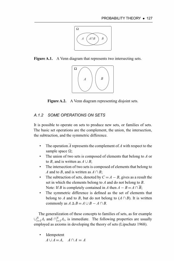
PROBABILITY THEORY • 127
BA A∩B
Ω
Figure A.1. A Venn diagram that represents two intersecting sets.
Ω
A B
Figure A.2. A Venn diagram representing disjoint sets.
A.1.2 SOME OPERATIONS ON SETS
It is possible to operate on sets to produce new sets, or families of sets.The basic set operations are the complement, the union, the intersection,the subtraction, and the symmetric difference.
• The operation A represents the complement of A with respect to thesample space �;
• The union of two sets is composed of elements that belong to A orto B, and is written as A ∪ B;
• The intersection of two sets is composed of elements that belong toA and to B, and is written as A ∩ B;
• The subtraction of sets, denoted by C=A− B, gives as a result theset in which the elements belong to A and do not belong to B.Note: If B is completely contained in A then A− B=A ∩ B;
• The symmetric difference is defined as the set of elements thatbelong to A and to B, but do not belong to (A ∩ B). It is writtencommonly as A � B=A ∪ B− A ∩ B.
The generalization of these concepts to families of sets, as for example∪N
i=1Ai and ∩Ni=1Ai, is immediate. The following properties are usually
employed as axioms in developing the theory of sets (Lipschutz 1968).
• IdempotentA ∪ A=A, A ∩ A = A

128 • INFORMATION THEORY
Ω
AAi
Figure A.3. Increasing sequence of sets.
Ω
A Ai
Figure A.4. Decreasing sequence of sets.
• Associative(A ∪ B) ∪ C=A ∪ (B ∪ C), (A ∩ B) ∩ C=A ∩ (B ∩ C)
• CommutativeA ∪ B=B ∪ A, A ∩ B=B ∩ A
• DistributiveA ∪ (B ∩ C)= (A ∪ B) ∩ (A ∪ C),A ∩ (B ∪ C)= (A ∩ B) ∪ (A ∩ C)
• IdentityA ∪ ∅=A, A ∩ U =AA ∪ U =U , A ∩ ∅=∅
• Complementary
A ∪ A=U , A ∩ A=∅ (A)=AU =∅, ∅=U
• de Morgan lawsA ∪ B=A ∩ B, A ∩ B=A ∪ B
A.1.3 FAMILIES OF SETS
The concept of family is important to characterize finite or infinite combi-nations of sets.The increasing sequence of sets, such that limi→∞∪Ai=A,is one of the most useful families of sets. This sequence is used in proofsof limits over sets.
The decreasing sequence of sets is defined in a similar manner, aslimi→∞∩ Ai=A, and is also used in proofs of limits over sets.

PROBABILITY THEORY • 129
A.1.4 INDEXING OF SETS
The Cartesian product is useful to express the idea of indexing of sets.Indexing expands the possibilities for the use of sets, and permits to gen-erate new entities, such as vectors and signals.
Example: consider Ai={0, 1}. Starting from this set it is possible to con-struct an indexed sequence of sets by defining its indexing: {AiεI }, I ={0, . . . , 7}. This family of indexed sets Ai constitutes a finite discretesequence, that is, a vector.
Example: again, let Ai={0, 1}, but now use I =Z, the set of positiveand negative integers plus zero. It follows that {AiεZ }, which represents aninfinite series of 0s and 1s, that is, it represents a binary digital signal. Forexample, · · · 0011111000 · · · .Example: using the same set Ai={0, 1}, but now indexing over the set ofreal numbers, {AiεI }, in which I =R, it is possible to form a signal whichis discrete in amplitude but continuous in time.
Example: considering A=R and I =R, the resulting set represents ananalog signal—a signal that is continuous in time and in amplitude.
A.1.5 AN ALGEBRA OF SETS
For the construction of an algebra of sets or, equivalently, for the con-struction of a field over which operations involving sets make sense, a fewproperties have to be obeyed.
1. If A∈F then A∈F . A is the set containing desired results, or overwhich one wants to operate;
2. If A∈F and B∈F then A ∪ B∈F .
The properties guarantee the closure of the algebra with respect to finiteoperations over sets. It is noticed that the universal set � always belongs tothe algebra, that is, �∈F , because �=A ∪ A. The empty set also belongsto the algebra, that is, ∅∈F , since ∅=�, follows by property 1.
Example: the family {∅, �} complies with the above properties and there-fore represents an algebra. In this case, ∅= {} and ∅=�. The union is alsorepresented, as can be easily checked.
Example: given the sets {CH } and {CT }, representing the faces of a coin,respectively, if {CH } ∈F then {CH }= {CT } ∈F . It follows that {CH , CT } ∈F⇒�∈F⇒∅∈F .
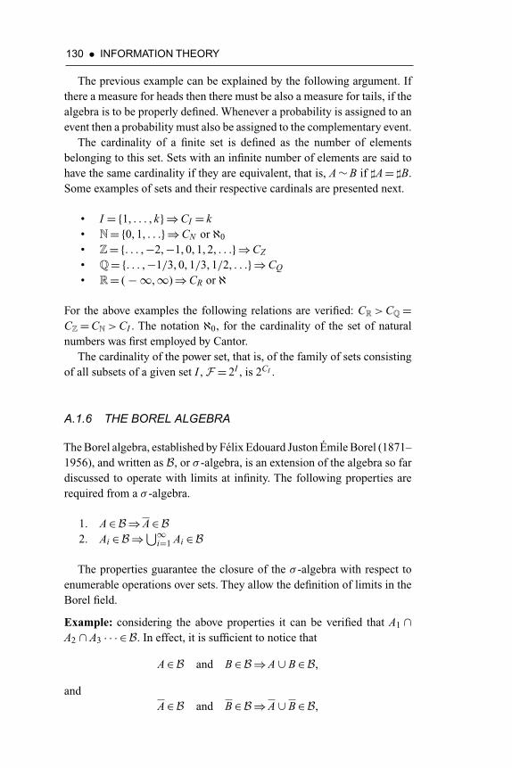
130 • INFORMATION THEORY
The previous example can be explained by the following argument. Ifthere a measure for heads then there must be also a measure for tails, if thealgebra is to be properly defined. Whenever a probability is assigned to anevent then a probability must also be assigned to the complementary event.
The cardinality of a finite set is defined as the number of elementsbelonging to this set. Sets with an infinite number of elements are said tohave the same cardinality if they are equivalent, that is, A∼B if �A= �B.Some examples of sets and their respective cardinals are presented next.
• I ={1, . . . , k}⇒CI = k• N={0, 1, . . .}⇒CN or ℵ0
• Z={. . . ,−2,−1, 0, 1, 2, . . .}⇒CZ
• Q={. . . ,−1/3, 0, 1/3, 1/2, . . .}⇒CQ
• R= (−∞,∞)⇒CR or ℵ
For the above examples the following relations are verified: CR > CQ=CZ=CN > CI . The notation ℵ0, for the cardinality of the set of naturalnumbers was first employed by Cantor.
The cardinality of the power set, that is, of the family of sets consistingof all subsets of a given set I , F = 2I , is 2CI .
A.1.6 THE BOREL ALGEBRA
The Borel algebra, established by Félix Edouard Juston Émile Borel (1871–1956), and written as B, or σ -algebra, is an extension of the algebra so fardiscussed to operate with limits at infinity. The following properties arerequired from a σ -algebra.
1. A∈B⇒A∈B2. Ai ∈B⇒⋃∞i=1 Ai ∈B
The properties guarantee the closure of the σ -algebra with respect toenumerable operations over sets. They allow the definition of limits in theBorel field.
Example: considering the above properties it can be verified that A1 ∩A2 ∩ A3 · · · ∈B. In effect, it is sufficient to notice that
A∈B and B∈B⇒A ∪ B∈B,
andA∈B and B∈B⇒A ∪ B∈B,
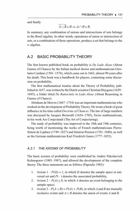
PROBABILITY THEORY • 131
and finally
A ∪ B∈B⇒A ∩ B ∈B.
In summary, any combination of unions and intersections of sets belongsto the Borel algebra. In other words, operations of union or intersection ofsets, or a combination of these operations, produce a set that belongs to theσ -algebra.
A.2 BASIC PROBABILITY THEORY
The first known published book on probability is De Ludo Aleae (AboutGames of Chance) by the Italian medical doctor and mathematician Giro-lamo Cardano (1501–1576), which came out in 1663, almost 90 years afterhis death. This book was a handbook for players, containing some discus-sion on probability.
The first mathematical treatise about the Theory of Probability, pub-lished in 1657, was written by the Dutch scientist Christian Huygens (1629–1695), a folder titled De Ratiociniis in Ludo Aleae (About Reasoning inGames of Chance).
Abraham de Moivre (1667–1754) was an important mathematician whoworked on the development of ProbabilityTheory. He wrote a book of greatinfluence in his time called Doctrine of Chances. The law of large numberswas discussed by Jacques Bernoulli (1654–1705), Swiss mathematician,in his work Ars Conjectandi (The Art of Conjecturing).
The study of probability was improved in the 18th and 19th centuries,being worth of mentioning the works of French mathematicians Pierre-Simon de Laplace (1749–1827) and Siméon Poisson (1781–1840), as wellas the German mathematician Karl Friedrich Gauss (1777–1855).
A.2.1 THE AXIOMS OF PROBABILITY
The basic axioms of probability were established by Andrei NikolaevichKolmogorov (1903–1987), and allowed the development of the completetheory. The three statements are as follows (Papoulis 1983):
1. Axiom 1 – P(�)= 1, in which � denotes the sample space or uni-versal set and P( · ) denotes the associated probability;
2. Axiom 2 – P(A)≥ 0, in which A denotes an event belonging to thesample space;
3. Axiom 3 – P(A ∪ B)=P(A)+ P(B), in which A and B are mutuallyexclusive events and A ∪ B denotes the union of events A and B.

132 • INFORMATION THEORY
Kolmogorov established a firm mathematical basis on which other the-ories rely, including the Theory of Stochastic Processes, the Communica-tions Theory, and the Information Theory, that use his axiomatic approachto Probability Theory.
Kolmogorov’s fundamental work was published in 1933 in Russian,and soon afterwards was translated to German with the title Grundbegriffeder Wahrscheinlichkeits Rechnung (Fundamentals of Probability Theory)(James 1981). In this work, Kolmogorov managed to combine AdvancedSet Theory, developed by Cantor, with Measure Theory, established byLebesgue, to produce what to this date is the modern approach to Proba-bility Theory.
The application of the axioms makes it possible to deduce all resultsrelative to Probability Theory. For example, the probability of the emptyset, ∅= {}, is easily calculated as follows. First it is noticed that
∅ ∪�=�,
since the sets ∅ and � are disjoint. Thus, it follows that
P(∅ ∪�)=P(�)=P(∅)+ P(�)= 1⇒P(∅)= 0.
In the case of sets A and B which are not disjoint, it follows that
P(A ∪ B)=P(A)+ P(B)− P(A ∩ B).
A.2.2 BAYES’ RULE
Bayes’ rule, which is essential for the development of Information Theory,concerns the computation of conditional probabilities and can be expressedby the following definition,
P(A|B)= P(A ∩ B)
P(B),
assuming P(B) �= 0.An equivalent manner of expressing the same result is the following,
P(A ∩ B)=P(A|B) · P(B), P(B) �= 0.
Some important properties of sets are presented next, in which A and Bdenote events from a given sample space.
• If A is independent of B, then P(A|B)=P(A). It then follows thatP(B|A)=P(B) and that B is independent of A.
• If B⊂A, then P(A|B)= 1.
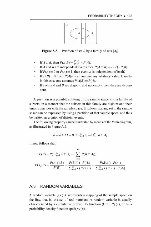
PROBABILITY THEORY • 133
Ω
AiB
Figure A.5. Partition of set B by a family of sets {Ai}.
• If A⊂B, then P(A|B)= P(A)P(B) ≥P(A).
• If A and B are independent events then P(A ∩ B)=P(A) · P(B).• If P(A)= 0 or P(A)= 1, then event A is independent of itself.• If P(B)= 0, then P(A|B) can assume any arbitrary value. Usually
in this case one assumes P(A|B)=P(A).• If events A and B are disjoint, and nonempty, then they are depen-
dent.
A partition is a possible splitting of the sample space into a family ofsubsets, in a manner that the subsets in this family are disjoint and theirunion coincides with the sample space. It follows that any set in the samplespace can be expressed by using a partition of that sample space, and thusbe written as a union of disjoint events.
The following property can be illustrated by means of the Venn diagram,as illustrated in Figure A.5.
B=B ∩�=B ∩ ∪Mi=1Ai=∪N
i=1B ∩ Ai.
It now follows that
P(B)=P( ∪Ni=1 B ∩ Ai)=
N∑i=1
P(B ∩ Ai),
P(Ai|B)= P(Ai ∩ B)
P(B)= P(B|Ai) · P(Ai)∑N
i=1 P(B ∩ Ai)= P(B|Ai) · P(Ai)∑N
i=1 P(B|Ai) · P(Ai).
A.3 RANDOM VARIABLES
A random variable (r.v.) X represents a mapping of the sample space onthe line, that is, the set of real numbers. A random variable is usuallycharacterized by a cumulative probability function (CPF) PX (x), or by aprobability density function (pdf) pX (x).
134 • INFORMATION THEORY
Example: a random variable with a uniform pdf, in the interval[0, 1], is described by the formula pX (x)= u(x)− u(x − 1). It follows, byAxiom 1, that ∫ +∞
−∞pX (x)dx= 1. (A.1)
In general, for a given probability distribution, the probability that Xbelongs to the interval (a, b] is given by
P(a < x≤ b)=∫ b
apX (x)dx. (A.2)
The cumulative probability function PX (x), of a random variable X , isdefined as the integral of pX (x),
PX (x)=∫ x
−∞pX (t)dt. (A.3)
A.3.1 EXPECTED VALUE OF A RANDOM VARIABLE
Let f (X ) denote a function of a random variable X . The average value, orexpected value, of the function f (X ) with respect to X is defined as
E[f (X )]=∫ +∞−∞
f (x)pX (x)dx. (A.4)
The following properties of the expected value follow from (A.4).
E[αX ]=αE[X ], (A.5)
E[X + Y ]=E[X ]+ E[Y ] (A.6)
and if X and Y are independent random variables then
E[XY ]=E[X ] · E[Y ]. (A.7)
A.3.2 MOMENTS OF A RANDOM VARIABLE
The kth moment of a random variable X is defined as
mk =E[X k ]=∫ +∞−∞
xk pX (x)dx. (A.8)

PROBABILITY THEORY • 135
Various moments of X have special importance and physical interpre-tation, as defined in the following:
• E[X ], arithmetic mean, average value, average voltage, statisticalmean;
• E[X 2], quadratic mean, total power;• E[X 3], measure of asymmetry of the pdf;• E[X 4], measure of flatness of the pdf.
A.3.3 VARIANCE OF A RANDOM VARIABLE
The variance of a random variable X is an important quantity in commu-nication theory, usually meaning AC power, and defined as follows,
V [X ]= σ 2X =E[(X − E[X ])2]. (A.9)
The standard deviation σX is defined as the square root of the variance of X .
A.3.4 CHARACTERISTIC FUNCTION
The characteristic function PX (w), also called moment generating func-tion, of a random variable X is usually defined based on the Fourier trans-form of the pdf of X , which is equivalent to substitute f (x)= e−jωx in (A.4),that is,
PX (w)=E[e−jωx]=∫ +∞−∞
e−jωxpX (x)dx, in which j=√−1. (A.10)
The statistical moments of a random variable X can also be obtaineddirectly from then characteristic function, as follows,
mi= 1
(− j)i
∂ iPX (w)
∂wi
∣∣∣w=0
. (A.11)
Given that X is a random variable, it follows that Y = f (X ) is also arandom variable, obtained by the application of the transformation f ( · ).The pdf of Y is related to that of X by the formula (Blake 1987)
pY (y)= pX (x)
|dy/dx|∣∣∣x=f −1(y)
, (A.12)
in which f −1( · ) denotes the inverse function of f ( · ).This formula assumesthe existence of the inverse function of f ( · ) as well as its derivative in allpoints.
136 • INFORMATION THEORY
A.3.4.1 Two Important Distributions
1. Gaussian random variableThe random variable X with pdf
pX (x)= 1
σX√
2πe− (x−mX )2
2σ2X (A.13)
is called a Gaussian (or Normal) random variable. The Gaussianrandom variable plays an extremely important role in engineering,considering that many well-known processes can be described orapproximated by this pdf. The noise present in either analog or dig-ital communications systems usually can be considered Gaussianas a consequence of the influence of many factors (Leon-Garcia1989). In Formula (A.13), mX represents the average value and σ 2
Xrepresents the variance of X .
2. Sinusoidal random variable
A sinusoidal tone X (t)=V cos (ω0t + φ), in which V represents aconstant amplitude, ω0 is a constant frequency, and φ is a uniformlydistributed random variable, has the following pdf
pX (x)= 1
π√
V 2 − x2, |x|< V . (A.14)
A.3.5 JOINT RANDOM VARIABLES
Consider that X and Y represent a pair of real random variables, with jointpdf pXY (x, y), as illustrated in Figure A.6. The probability of x and y beingsimultaneously in the region defined by the polygon [abcd] is given by theexpression (Alencar 2014).
Prob(a < x < b, c < y < d)=∫ b
a
∫ d
cpXY (x, y)dxdy. (A.15)
The individual pdf’s of X and Y , also called marginal distributions,result from the integration of the joint pdf as follows,
pX (x)=∫ +∞−∞
pXY (x, y)dy, (A.16)
and
pY (y)=∫ +∞−∞
pXY (x, y)dx. (A.17)

PROBABILITY THEORY • 137
0
pXY(x,y)
X
y
Figure A.6. Joint probability density function.
The joint average E[f (X , Y )] is calculated as
E[f (X , Y )]=∫ +∞−∞
∫ +∞−∞
f (x, y)pXY (x, y)dxdy, (A.18)
for an arbitrary function f (X , Y ) of X and Y .The joint moments mik , of order ik , are calculated as
mik =E[X i, Y k ]=∫ +∞−∞
∫ +∞−∞
xiyk pXY (xy)dxdy. (A.19)
The two-dimensional characteristic function is defined as the two-dimensional Fourier transform of the joint probability density pXY (x, y)
PXY (ω, ν)=E[e−jωX−jνY ]. (A.20)
When the sum Z =X + Y of two statistically independent r.v.’s is con-sidered, it is noticed that the characteristic function of Z turns out to be
PZ (ω)=E[e−jωZ ]=E[e−jω(X+Y )]=PX (ω) · PY (ω). (A.21)
As far as the pdf of Z is concerned, it can be said that
pZ (z)=∫ ∞−∞
pX (ρ)pY (z − ρ)dρ, (A.22)
or
pZ (z)=∫ ∞−∞
pX (z − ρ)pY (ρ)dρ. (A.23)

138 • INFORMATION THEORY
Equivalently, the sum of two statistically independent r.v.’s has a pdfgiven by the convolution of the respective pdf’s of the r.v.’s involved inthe sum.
The random variables X and Y are called uncorrelated if E[XY ]=E[X ] ·E[Y ]. The criterion of statistical independence of random variables, whichis stronger than correlation, is satisfied if pXY (x, y)= pX (x) · pY (y).
REFERENCES
Abramowitz, M., and I.A. Stegun, eds. 1965. Handbook of MathematicalFunctions. New York: Dover Publications Inc.
Abramson, N. 1963. Information Theory and Coding. New York:McGraw-Hill.
Aczél, J., and Z. Daróczy. 1975. On Measures of Information and TheirCaracterizations. New York: Academic Press.
Adke, S.R., and S.M. Manjunath. 1984. An Introduction to Finite MarkovProcesses. New Delhi: John Wiley and Sons.
Ahlswede, R. 1971. “Multi-way Communication Channels.” In Proceed-ings of the 2nd International Symposium on Information Theory,pp. 103–35. Tsahkad-sor, USSR: Akadémiai Kiadó..
Alencar, M.S. 1992a. “The Capacity Region for the Gaussian Channel withRandom Multipath.” In Proceedings of the Third IEEE InternationalSymposium on Personal, Indoor and Mobile Radio Communications –PIMRC’92, pp. 483–87. Boston, MA.
Alencar, M.S. 1992b. “The Capacity Region of the Non-Cooperative Multi-pleAccess Channel with Rayleigh Fading.” In Proceedings of theAnnualConference of the Canadian Institute forTelecommunications Research,pp. 45–46. Sainte Adèle, Canada.
Alencar, M.S. 2014. Teoria de Conjuntos, Medida e Probabilidade. SãoPaulo, Brasil: Edi-toraÉrica Ltda. ISBN 978-85-365-0715-6.
Alencar, M.S., and I.F. Blake. 1993a. “Analysis of the Capacity for aMarkovian Multiple Access Channel.” In IEEE Pacific Rim Confer-ence on Communications, Computers and Signal Processing, pp. 81–84.Victoria, Canada.
Alencar, M.S., and I.F. Blake. 1993b. “Analysis of the Capacity Regionfor the Non-Cooperative Multiaccess Channel with Rician Fading.” InIEEE International Conference on Communications – ICC’93, pp. 282–86. Geneva, Switzerland.
139

140 • REFERENCES
Alencar, M.S., and I.F. Blake. 1993c. “The Capacity of a Code DivisionMultiple Access Channel.” In 1993 International Symposium on 139Communications – ISCOM’93, Vol.1, pp. 1.1–1.9. Hsinchu,Taiwan.
Ash, R.B. 1965. Information Theory. New York: Dover Publications Inc.Bierbaum, M., and H.-M.Wallmeier. 1979. “A Note on the Capacity Region
of the Multiple Access Channel.” IEEE Transactions on InformationTheory 25, no. 4, p. 484. doi: http://dx.doi.org/10.1109/tit.1979.1056064
Blahut, R.E. 1987. Principles and Practice of InformationTheory. Reading,MA: Addison-Wesley Publishing Co.
Blahut, R.E. 1990. Digital Transmission of Information. Reading, MA:Addison-Wesley Publishing Co.
Blake, I.F. 1987. An Introduction to Applied Probability. Malabar, FL:Robert E. Krieger Publishing Co.
Blake, I.F., and R.C. Mullin. 1976. An Introduction to Algebraic and Com-binatorial Coding Theory. New York: Academic Press Inc.
Borth, D.E., and M.B. Pursley. 1979. “Analysis of Direct-Sequence Spread-Spectrum Multiple-Access Communications OverRician Fading Chan-nels.” IEEE Transactions on Communications 27, no. 10, pp. 1566–77.doi: http://dx.doi.org/10.1109/tcom.1979.1094291
Boyer, C. 1974. História da Matemática. São Paulo, Brasil: Editora EdgardBlucher Ltda.
Brady, D.P. 1991. “A Semiclassical Analysis of Optical Code DivisionMultiple Access.” IEEE Transactions on Communications 39, no. 1,pp. 85–93. doi: http://dx.doi.org/10.1109/26.68279
Cheng, R.S., and S. Verdú. 1991. “The Effect of Asynchronism on theTotal Capacity of Gaussian Multiple-access Channels.” In Proceedingsof the IEEE International Symposium on Information Theory, p. 211.Budapest, Hungary.
Chung, H., and P.V. Kumar. 1990. “Optical Orthogonal Codes – NewBounds and an Optimal Construction.” IEEE Transactions on Infor-mation Theory 36, no. 4, pp. 866–73. doi: http://dx.doi.org/10.1109/18.53748
Cook, C.E., F.W. Ellersick, L.B. Milstein, and D.L. Schilling. 1983. Spread-Spectrum Communications. New York: IEEE Press.
Cook, C.E., and H.S. Marsh. 1983. “An Introduction to Spread Spec-trum.” IEEE Communications Magazine 21, no. 2, pp. 8–16. doi: http://dx.doi.org/10.1109/mcom.1983.1091346
Cover, T.M. 1972. “Broadcast Channels.” IEEE Transactions on Infor-mation Theory 18, no. 1, pp. 2–14. doi: http://dx.doi.org/10.1109/tit.1972.1054727

REFERENCES • 141
Cover, T.M., R.J. McEliece, and E.C. Posner. 1981. “AsynchronousMultiple-Access Channel Capacity.” IEEETransactions on InformationTheory 27, no. 4, pp. 409–13. doi: http://dx.doi.org/10.1109/tit.1981.1056382
Csiszár, I., and J. Kórner. 1981. Information Theory: Coding Theorems forDiscrete Memoryless Systems. New York: Academic Press.
Dixon, R.C. 1984. Spread Spectrum Systems. New York: John Wiley &Sons.
Dobrushin, R.L. 1961. “Mathematical Problems in the Shannon Theory ofOptimal Coding of Information.” In Proceedings of the 4th BerkeleySymposium on Mathematics, Statistics and Probability, Vol. 1, pp. 211–52. Berkeley, CA.
Elliott, E.O. 1965. “A Model of the SwitchedTelephone Network for DataCommunications.” The Bell System Technical Journal 44, no. 1, pp. 88–109. doi: http://dx.doi.org/10.1002/j.1538-7305.1965.tb04139.x
Ericson, T. 1970. “A Gaussian Channel with Slow Fading.” IEEE Trans-actions on Information Theory 16, no. 3, pp. 353–55. doi: http://dx.doi.org/10.1109/tit.1970.1054448
Feinstein, A. 1958. Foundations of Information Theory. New York:McGraw-Hill Book Company Inc.
Fritchman, B.D. 1967. “A Binary Channel Characterization Using Parti-tioned Markov Chains.” IEEE Transactions on Information Theory 13,no. 2, pp. 221–27. doi: http://dx.doi.org/10.1109/tit.1967.1053975
Gaarder, N.T., and J.K. Wolf. 1975. “The Capacity of a Multiple-AccessDiscrete Memoryless Channel Can Increase with Feedback.” IEEETrans-actions on Information Theory 21, no. 1, pp. 100–02. doi: http://dx.doi.org/10.1109/tit.1975.1055312
Gallager, R.G. 1968. Information Theory and Reliable Communication.New York: John Wiley and Sons Inc.
Gallager, R.G. 1985. “A Perspective on Multiaccess Channels.”IEEETrans-actions on Information Theory 31, no. 2, pp. 124–42. doi: http://dx.doi.org/10.1109/tit.1985.1057022
Geraniotis, E.A., and B. Ghaffari. 1991. “Performance of Binary and Qua-ternary Direct-Sequence Spread Spectrum Multiple-Access Systemswith Random Signature Sequences.” IEEE Transactions on Communi-cations 39, no. 5, pp. 713–24. doi: http://dx.doi.org/10.1109/26.87162
Geraniotis, E.A., and M.B. Pursley. 1985. “Performance of CoherentDirect-Sequence Spread Spectrum Communications Over SpecularMultipath Fading Channels.” IEEE Transactions on Communications33, no. 6, pp. 502–08. doi: http://dx.doi.org/10.1109/tcom.1985.1096335
142 • REFERENCES
Geraniotis, E.A., and M.B. Pursley. 1986. “Performance of Noncoher-ent Direct-Sequence Spread Spectrum Communications over SpecularMultipath Fading Channels.” IEEE Transactions on Communications34, no. 6, pp. 219–26. doi: http://dx.doi.org/10.1109/tcom.1986.1096528
Gilbert, E.N. 1960. “Capacity of a Burst-Noise Channel.” The Bell SystemTechnical Journal 39, no. 5, pp. 1253–65. doi: http://dx.doi.org/10.1002/j.1538-7305.1960.tb03959.x
Gilhousen, K.S., I.M. Jacobs, R. Padovani, A.J. Viterbi, L.A. Weaver, andC.E. Wheatley. 1991. “On the Capacity of a Cellular CDMA System.”IEEE Transactions on Vehicular Technology 40, no. 2, pp. 303–12. doi:http://dx.doi.org/10.1109/25.289411
Gold, R. 1967. “Optimal Binary Sequences for Spread Spectrum Multi-plexing.” IEEE Transactions on Information Theory 13, no. 4, pp. 619–21. doi: http://dx.doi.org/10.1109/tit.1967.1054048
Gradshteyn, I.S., and I.M. Ryzhik. 1990. Table of Integrals, Series, andProducts. San Diego, CA: Academic Press Inc.
Halmos, P.R. 1960. Naive Set Theory. Princeton, NJ: D. Van NostrandCompany Inc.
Hartley, R.V.L. 1928. “Transmission of Information.” Bell SystemsTech-nical Journal p. 535. doi: http://dx.doi.org/10.1002/j.1538-7305.1928.tb01236.x
Haykin, S. 1988. Digital Communications. NewYork: JohnWiley and Sons.Haykin, S. 1999. The Code Book – The Science of Secrecy from Ancient
Egypt to Quantum Cryptography. New York: Doubleday.Holtzman, J.M. 1992. “A Simple, Accurate Method to Calculate Spread-
Spectrum Multiple-Access Error Probabilities.” IEEE Transactions onCommunications 40, no. 3, pp. 461–64. doi: http://dx.doi.org/10.1109/26.135712
Hui, J.Y.N. 1984a. “Multiple Accessing for the Collision ChannelWithout Feedback.” IEEE Journal on Selected Areas in Communica-tions 2, no. 4, pp. 575–82. doi: http://dx.doi.org/10.1109/jsac.1984.1146089
Hui, J.Y.N. 1984b. “Throughput Analysis for Code Division MultipleAccessing of the Spread Spectrum Channel.” IEEE Journal on SelectedAreas in Communications 2, no. 4, pp. 482–86. doi: http://dx.doi.org/10.1109/jsac.1984.1146083
Hui, J.Y.N., and P.A. Humblet. 1985. “The Capacity Region of the TotallyAsynchronous Multiple-Access Channel.” IEEE Transactions on Infor-mation Theory 31, no. 2, pp. 207–16.
James, B.R. 1981. Probabilidade: Um CursoEmNívelIntermediário. CNPq,Rio de Janeiro, Brasil: Instituto de MatemáticaPura e Aplicada.

REFERENCES • 143
Kavehrad, M., and P.J. McLane. 1985. “Performance of Low-ComplexityChannel Coding and Diversity for Spread Spectrum in Indoor, WirelessCommunication.” AT&T Technical Journal 64, no. 8, pp. 1927–64.
Kavehrad, M., and P.J. McLane. 1987. “Spread Spectrum for Indoor DigitalRadio.” IEEE Communications Magazine 25, no. 6, pp. 32–40.
Kavehrad, M., and B. Ramamurthi. 1987. “Direct Sequence SpreadSpectrum with DPSK Modulation and Diversity for Indoor WirelessCommunications.” IEEE Transactions on Communications 35, no. 2,pp. 224–36.
Khinchin, A.I. 1957. Mathematical Foundations of Information Theory.New York: Dover Publications, Inc.
Kleinrock, L. 1975. Queueing Systems. New York: John Wiley & Sons.Komo, J.J., and S.C. Liu. 1990. “Maximal Length Sequences for Frequency
Hopping.” IEEE Journal on Selected Areas in Communications 8, no. 5,pp. 819–22.
Lee, W.C.Y. 1990. “Estimate of Channel Capacity in Rayleigh FadingEnvironment.” IEEE Transactions on Vehicular Technology 39, no. 3,pp. 187–89.
Lee, W.C.Y. 1991. “Overview of Cellular CDMA.” IEEE Transactions onVehicular Technology 40, no. 2, pp. 291–302.
Leon-Garcia, A. 1989. Probability and Random Processes for ElectricalEngineering. Reading, Massachusetts: Addison-Wesley Publishing Co.
Lipschutz, S. 1968. Teoria de Conjuntos. Rio de Janeiro, Brasil: Ao LivroTécnico S.A.
MacKay, D.J.C. 2003. Information Theory, Inference, and Learning Algo-rithms. Cambridge, UK: Cambridge University Press.
Mandell, M., and R. McEliece. 1991. Some Properties of Memory-lessMultiterminal Interference Channels. Proceedings of the IEEE Inter-national Symposium Information Theory, p. 212. Budapest, Hungary:IEEE.
Massey, J.L. 1990. The Relevance of Information Theory to ModernCryptography. Proceedings of the Bilkent International Conference onNew Trends in Communications, Control and Signal Processing(NILCON’90), pp. 176–82. Ankara, Turkey: Elsevier Science Publisher.
Maurer, U.M. 1989.A Provably-Secure Strongly-Randomized Cipher. Pro-ceedings of the Monte Verita Seminar on Future Directions in Cryptog-raphy. Ascona, Switzerland.
Misser, H.S., C.A.F.J. Wijffels, and R. Prasad. 1991. “Throughput Analysisof CDMA with DPSK Modulation and Diversity in Indoor Rician FadingRadio Channels.” Electronics Letters 27, no. 7, pp. 601–603.
Nyquist, H. 1924. “Certain Factors Affecting Telegraph Speed.” Bell Sys-tems Technical Journal, 3, p. 324.

144 • REFERENCES
Oberhettinger, F. 1990. Tables of Fourier Transforms and Fourier Trans-forms of Distributions. Berlin, Germany: Springer-Verlag.
Ozarow, L.H., and A.D. Wyner. 1990. “On the Capacity of the GaussianChannel with a Finite Number of Input Levels.” IEEE Transactions onInformation Theory 36, no. 6, pp. 1426–28.
Papoulis, A. 1983. “Random Modulation: A Review.” IEEE Transactionson Acoustics, Speech and Signal Processing 31, no. 1, pp. 96–105.
Pickholtz, R.L., D.L. Schilling, and L.B. Milstein. 1982. “Theory ofSpread–Spectrum Communications—A Tutorial.” IEEE Transactionson Communications, COM 30, no. 5, pp. 855–84.
Pierce, J.R. 1980.An Introduction to InformationTheory—Symbols, Signals& Noise. 2nd ed. New York: Dover Publications Inc.
Proakis, J.G. 1989. Digital Communications. McGraw-Hill.Pursley, M.B. 1977. “Performance Evaluation for Phase-Coded Spread
Spectrum Multiple-Access Communications—Part I: System Analy-sis.” IEEE Transactions on Communications 25, no. 8, pp. 795–99.
Reza, F.M. 1961. An Introduction to Information Theory. New York:McGraw-Hill Book Co.
Ricciardi, L.M. 1990. Lectures in Applied Mathematics and Informatics.Manchester, UK: Manchester University Press.
Sadowsky, J.S., and R.K. Bahr. 1991. “Direct-Sequence Spread-SpectrumMultiple-Access Communications with Random Signature Sequences:A Large Deviations Analysis.” IEEE Transactions on Information The-ory 37, no. 3, pp. 514–27.
Sarwate, D.V. and M.B. Pursley. 1980. “Crosscorrelation Properties ofPseudorandom and Related Sequences.” Proceedings of the IEEE 68,no. 5, pp. 593–619.
Sayood, K. 2006. Introduction to Data Compression. San Francisco, CA:Morgan Kaufmann.
Schilling, D.L., L.B. Milstein, R.L. Pickholtz, M. Kullback, and F. Miller.1991. “Spread Spectrum for Commercial Communications.” IEEE Com-munications Magazine 29, no. 4, pp. 66–79.
Scholtz, R.A. 1982. “The Origins of Spread-Spectrum Communications.”IEEE Transactions on Communications, COM 30, no. 5, pp. 822–54.
Schwartz, M. 1970. Information Transmission, Modulation, and Noise.New York: McGraw-Hill.
Shannon, C.E. 1948. “A Mathematical Theory of Communication.” TheBell System Technical Journal 27, pp. 379–423.
Shannon, C.E. 1961. “Two-way Communications Channels.” Proceed-ings of the 4th Berkeley Symposium on Mathematics, Statistics andProbability, Vol. 1, pp. 611–44. Berkeley, CA: University of CaliforniaPress.

REFERENCES • 145
Shamai, S., L.H. Ozarow, and A.D. Wyner. 1991. “Information Rates fora Discrete-Time Gaussian Channel with Intersymbol Interference andStationary Inputs.” IEEE Transactions on Information Theory 37, no. 6,pp. 1527–39.
Simon, M.K., J.K. Omura, R.A. Scholtz, and B.K. Levitt. 1985. Vol. 1.Spread Spectrum Communications. Rockville, MD: Computer SciencePress.
Sommer, R.C. 1966. “Asynchronously Multiplexed Channel Capacity.”Proceeding of the IEEE 54, no. 1, pp. 79–80.
Soroushnejad, M., and E. Geraniotis. 1991. “Probability of Capture andRejection of Primary Multiple-Access Interference in Spread-Spectrum Networks.” IEEE Transactions on Communications 39, no. 6,pp. 986–94.
Sousa, E.S. 1989. “Throughput of Spread-Spectrum Systems with a LargeNumber of Users.” IEE Proceedings 136, no. 3, pp. 220–26.
Sousa, E.S. 1990. “Interference Modeling in a Direct-Sequence Spread-Spectrum Packet Radio Network.” IEEE Transactions on Communica-tions 38, no. 9, pp. 1475–82.
Sousa, E.S. 1992. “Performance of a Spread Spectrum Packet RadioNetwork Link in a Poisson Field of Interferers.” IEEE Transactionson Information Theory 38, no. 6, pp. 1743–54.
Stallings, W. 1999. Cryptography and Network Security—Principles andPractice. Upper Saddle River, NJ: Prentice Hall.
Tanenbaum, A.S. 2003. Computer Networks. Englewood Cliffs, NJ:Prentice-Hall, PTR.
Turin, G.L. 1980. “Introduction to Spread-Spectrum Antimultipath Tech-niques and Their Application to Urban Digital Radio.” Proceedings ofthe IEEE 68, no. 3, pp. 328–53.
Turin, G.L. 1984a. “Commutation Signaling—An Antimultipath Tech-nique.” IEEE Journal on Selected Areas in Communications 2, no. 4,pp. 548–62.
Turin, G.L. 1984b. “The Effects of Multipath and Fading on the Perfor-mance of Direct-Sequence CDMA Systems.” IEEE Journal on SelectedAreas in Communications 2, no. 4, pp. 597–603.
Van der Lubbe, J.C.A. 1997. Information Theory. Cambridge, UK: Cam-bridge University Press.
Verdú, S. 1986. “Minimum Probability of Error for AsynchronousGaussian Multiple-Access Channels.” IEEE Transactions on Informa-tion Theory 32, no. 1, pp. 85–96.
Verdú, S. 1989a. “Multiple-Access Channels with Memory with and with-out Frame Synchronism.” IEEETransactions on InformationTheory 35,no. 3, pp. 605–19.

146 • REFERENCES
Verdú, S. 1989b. “The Capacity Region of the SymbolAsynchronous Gaus-sian Multiple-Access Channel.” IEEETransactions on InformationThe-ory 35, no. 4, pp. 733–51.
Viterbi, A.J. 1985. “When Not to Spread Spectrum—A Sequel.” IEEECommunications Magazine 23, no. 4, pp. 12–17.
Viterbi, A.J. 1991. “Wireless Digital Communication: A View Based onThree Lessons Learned.” IEEE Communications Magazine 29, no. 9,pp. 33–36.
Wang, H.S. Finite-State Modeling, Capacity, and Joint Source/ChannelCoding for Time-Varying Channels. [PhD Thesis]. New Brunswick, NJ:Graduate School – New Brunswick Rutgers, The State University ofNew Jersey; 1992
Welch, L.R. 1974. “Lower Bounds on the Maximum Cross Correlation ofSignals”. IEEE Transactions on Information Theory, 20, no. 3,pp. 397–99.
Wozencraft, J.M., and B. Reiffen. 1961. Sequential Decoding. Cambridge,US: MIT Press.
Wyner, A.D. 1974. “Recent Results in the Shannon Theory”. IEEETransactions on Information Theory, 20, no. 1, pp. 2–9.
Yue, O.-C. 1983. “Spread Spectrum Mobile Radio, 1977–1982”. IEEETransactions on Vehicular Technology, 32, no. 1, pp. 98–105.
Zadeh, L.A. 1965. “Fuzzy Sets”. Information and Control, 8, no. 3,pp. 338–53.

ABOUT THE AUTHOR
Marcelo Sampaio de Alencar was born in Serrita, Brazil in 1957. Hereceived his bachelor s degree in Electrical Engineering from Federal Uni-versity of Pernambuco (UFPE), Brazil in 1980; his master degree fromFederal Universty of Paraiba (UFPB), Brazil 1988; and his PhD from Uni-versity of Waterloo, Canada in 1993. He is currently an emeritus memberof the Brazilian Telecommunications Society (SBrT), IEEE senior mem-ber, chair professor at the Department of Electrical Engineering, FederalUniversity of Campina Grande, Brazil. He also worked for the State Uni-versity of Santa Catarina (UDESC), Embratel, and University of Toronto,as isiting rofessor.
He is founder and president of the Institute for Advanced Studies inCommunications (Iecom). He has been awarded several scholarships andgrants, including three scholarships and several research grants from theBrazilian National Council for Scientific and Technological Research(CNPq), two grants from the IEEE Foundation, a scholarship from the Uni-versity of Waterloo, a scholarship from the Federal University of Paraiba,an achievement award for contributions to the Brazilian Telecommunica-tions Society (SBrT), an award from the Medicine College of the FederalUniversity of Campina Grande (UFCG), an achievement award from theCollege of Engineering of the Federal University of Pernambuco, and theMedal Professor Attilio Jose Giarola from the Brazilian Microwave andOptoelectronics Society (SBMO). He has published over 350 engineeringand scientific papers and 15 books. He is a columnist of the traditionalBrazilian newspaper Jornal do Commercio, and vice president for externalrelations, SBr .
147
’’s
pv
T


INDEX
AAbsolutely secure event, 124Algebra, 127, 129
Borel, 130closure, 129
Algebraic coding theory, 77Alzheimer, Aloysius, 32Appearance
equivocation, 121Asymmetric key, 120Axiom
choice, 126Peano, 126specification, 126
Axioms, 126Ayer, Alfred Jules,
BBelonging, 126Binary
Huffman, 27Bit, 17Bletchley Park, 117Borel
algebra, 130Borel, Félix Edouard Juston
Émile, 13BSC, 4
CCantor, Georg, 125Capacity
bound, 107channel, 41sum, 94
Cardinalnumber, 130numbers, 125
Cardinality, 130Carrier suppression, 80CDMA, 72, 76, 87
non-cooperative, 89performance analysis, 76,
90Channel
binary symmetric, 44communication, 34discrete, 43independent output, 36noiseless, 35noisy, 43non-cooperative, 89
Ciphertextentropy, 121
Clausius, Rudolph, 31Closure, 129CMOS, 17Code
chip rate, 88classification, 19comma, 21decision tree, 14
149
1
04

150 • INDEX
decoding tree, 15Huffman, 27instantaneous, 21, 23prefix, 14, 16
extended, 17uniquely decodable, 20
Codercodewords, 1source, 13
Codesblock, 19non-singular, 19
Codewords, 11Coding
efficiency, 12source, 11
Communicationspersonal, 71
Computer network, 118Cryptography, 72, 118
history, 117information theory, 121model, 119principles, 120uncertainty, 121
Cryptosystemabsolute security, 124information theory, 123
DDedekind, J. W. R., 125Direct sequence, 72Disjoint, 126DPSK, 87DS, 72DSSS, 78, 87
EEfficiency, 43Empty, 126Enigma, 117Entropy,
conditional, 34cryptography, 120cryptosystem, 122extended source, 12inequality, 37joint, 33, 39properties, 6relations, 37
Error probability, 109Extension
source, 12
FFading, 72Families, 128Fano, Robert, 27FDMA, 76FH, 72Fractals, 125Frequency hopping, 72Fuzzy set, 2
GGold sequence, 82
HHartley, Ralph Vinton Lyon, 1,
31Hilbert, David, 125Huffman
non-unicity, 29procedure, 28
Huffman, David, 27
IInclusion, 126Indexing, 129Inequality
Kraft, 24Kraft-McMillan, 16
Informationaverage mutual, 39
1
3
INDEX • 151
channel, 34entropy, 2, 3joint, 32measure of, 2mutual,semantics, 1theory, 1
Internetbackbone, 118protocol, 1
JJammer, 74
broad band noise, 74partial band, 74partial time, 74repeater, 74tone, 74
Jamming, 72Joint entropy
cryptosystem, 122Joint random Variables, 136
KKasami
sequence, 84Key
entropy, 120equivocation, 121
Khinchin, AleksandrYakovlevich, 2
Kolmogorov, AndreiNikolaevich, 31, 131
Kraftinequality, 24
Kraft-McMillaninequality, 16
Kronecker, Leopold, 125
LLaser, 18Lebesgue, Henri Léon, 40
MMAI, 78Matched filter, 91Maximal length
linear sequence, 80sequence, 79
Maximum likelihood receiver,91
Measure, 126Lebesgue, 40probability, 126
Messageequivocation, 121uncertainty, 121
Moments, 134Multipath, 72, 88Multiple access, 71
DSSS, 78interference, 78
NNon-cooperative channel, 89Non-repudiation, 118Nyquist, Harry, 1, 31
PPassword, 118PCN, 87Peano
axiom, 126Peirce, Charles Sanders, 1Personal communications, 71Photon, 17Pierce, John Robinson, 1Plaintext
entropy, 120Prefix
code, 14, 16Probability, 126
joint random variables, 136moments, 134random variables, 13
38
18
3

152 • INDEX
Probability theory, 133Pseudo-random, 80Public key infrastructure,
118
RRényi, Alfréd, 2Radiation
electromagnetic, 18Random variables, 13Rate
transmission, 43Redundancy, 12
absolute, 42relative, 43
SSchröder-Bernstein
theorem, 126Sequence
Gold, 82Kasami, 84maximal length, 81maximal-length, 79, 80Mersenne, 81Welsh bound, 82
Sequence design, 79Session
hijacking, 118Set, 125
algebra, 127disjoint, 126families, 128fuzzy, 2infinite, 125operations, 127universal, 126universal set, 125
Set theory, 125, 126Sets
algebra, 129indexing, 129
ShannonClaude Elwood, 39, 41first theorem, 12
Shannon, Claude Elwood,
Signalspace, 74
Sniffing, 118Source
efficiency, 12extended, 12
Source codingtheorem, 12
Spectralcompression, 75
Spoofing, 118Spread spectrum, 71
m-sequence, 79carrier suppression, 8direct sequence, 72DSSS, 87frequency hopping, 72interference, 77performance Analysis, 76pseudo-random, 80sequence design, 79time hopping, 73time-frequency hopping,
Substitution, 120Sum capacity, 94Symmetric key, 120
TTCP/IP, 118TDMA, 76TH, 73Theorem
Schröder-Bernstein, 126Time hopping, 73Transfinite arithmetic, 12
3
1, 31
0
78
5

INDEX • 153
Transformationcryptography, 119
Transposition, 120TTL, 17Turing, Alan Mathison, 117
UUniversal, 126University of Halle, 125
VVectorial
space, 74
Venndiagram, 126
Venn diagram, 126
WWelsh bound, 82
ZZadeh, Lotfi Asker, 2Zenon, 125Zorn
lemma, 126Zorn’s lemma, 126


FORTHCOMING TITLES IN OUR COMMUNICATIONS AND SIGNAL PROCESSING COLLECTION
Orlando Baiocchi, University of Washington Tacoma, Editor
Signal Integrity: The Art of Interconnect Design For High Speed and High Reliability Circuits by Joel Jorgenson
Cryptography Explained by Raj Katti
Momentum Press publishes several other collections, including: Industrial, Systems, and Innovation Engineering; Manufacturing and Processes; Engineering Management; Electrical
Power; Fluid Mechanics; Acoustical Engineering; Aerospace Engineering; Biomedical Engineering; and Healthcare Administration
Momentum Press is actively seeking collection editors as well as authors. For more information about becoming an MP author or collection editor, please visit
http://www.momentumpress.net/contact
Announcing Digital Content Crafted by Librarians
Momentum Press offers digital content as authoritative treatments of advanced engineering top-ics by leaders in their field. Hosted on ebrary, MP provides practitioners, researchers, faculty, and students in engineering, science, and industry with innovative electronic content in sensors and controls engineering, advanced energy engineering, manufacturing, and materials science.
Momentum Press offers library-friendly terms:
• perpetualaccessforaone-timefee• nosubscriptionsoraccessfeesrequired• unlimitedconcurrentusagepermitted• downloadablePDFsprovided• freeMARCrecordsincluded• freetrials
The Momentum Press digital library is very affordable, with no obligation to buy in future years.
Formoreinformation,pleasevisitwww.momentumpress.net/library or to set up a trial in the US, please contact [email protected].

Inform
ation Theo
ryA
LEN
CA
R
EBOOKS FOR THE ENGINEERING LIBRARYCreate your own Customized Content Bundle—the more books you buy, the greater your discount!
THE CONTENT• Manufacturing
Engineering• Mechanical
& Chemical Engineering
• Materials Science & Engineering
• Civil & Environmental Engineering
• Advanced Energy Technologies
THE TERMS• Perpetual access for
a one time fee• No subscriptions or
access fees• Unlimited
concurrent usage• Downloadable PDFs• Free MARC records
For further information, a free trial, or to order, contact: [email protected]
Information TheoryMarcelo S. AlencarInformation Theory covers the historical evolution of infor-mation theory, along with the basic concepts linked to information. It discusses the information associated to a cer-tain source and the usual types of source codes, information transmission, joint information, conditional entropy, mutual information, and channel capacity.
The hot topic of multiple access systems for cooperative and noncooperative channels is also discussed, along with code division multiple access (CDMA), the basic block of most cellular and personal communication systems, and the capacity of a CDMA system. Also presented is the information theoretical aspects of cryptography, which are important for network security, a topic intrinsically connected to computer networks and the Internet.
To help the reader understand the theory, the text also includes a review of probability theory, solved problems, illustrations, and graphics.
Marcelo Sampaio de Alencar received his bachelor‘s degree in Electrical Engineering from Federal University of Pernambuco (UFPE), Brazil in 1980; his master’s degree from Federal University of Paraiba (UFPB), Brazil in 1988; and his PhD from the University of Waterloo, Canada in 1993. He is currently emeritus member of the Brazilian Tele-communications Society (SBrT), IEEE senior member, chair professor at the Department of Electrical Engineering, Federal University of Campina Grande, Brazil. He is founder and president of the Institute for Advanced Studies in Communications (Iecom), and has been awarded several scholarships and grants including three scholarships and several research grants from the Brazilian National Council for Scientific and Technological Research (CNPq), two grants from the IEEE Foundation, a scholarship from the University of Waterloo, a scholarship from the Federal University of Paraiba, and many others. He has published over 350 engineering and scientific papers and 15 books.
Marcelo S. Alencar
Information Theory
COMMUNICATIONS AND SIGNAL PROCESSING COLLECTIONOrlando R. Baiocchi, Editor
ISBN: 978-1-60650-528-1