ALE Starter Guide - TI

Application ReportSLEA014 – MAY 2003

ALE STARTER GUIDEJim Coates (TI Dallas) Digital Audio Solutions

ABSTRACT

The automatic loudspeaker equalization (ALE) program supports the following Texas Instrumentsdigital audio processors

• TAS3001• TAS3002• TAS3004• TAS3103

This application note addresses the use of ALE in developing application-specific coefficients for theTAS3103 digital audio processor.

The TAS3103 digital audio processor is a three-channel audio processor. Many audio processingfeatures are provided in the TAS3103, including

• Up to sixteen biquad filters per channel for speaker equalization• Loudness compensation unique to each channel• Dynamic range compression / expansion

The automatic loudspeaker equalization (ALE) program provides a user-friendly environment in which tofully use the capability of the TAS3103 in a given application. Specifically, the ALE provides the ability to

• Develop equalization filters byo Specifying filter type(s) and parameterso Specifying a desired speaker response given a measured speaker response

• Tailor loudness compensation to achieve a specified audio presentation• Set dynamic range parameters

This application note consists of three major sections, with each section addressing one of the threepreviously listed capabilities.

Application ReportSLEA014 – MAY 2003t

Contents

Initial Setup Steps ..............................................................................................................................................4Filter Coefficient Generation ..............................................................................................................................5

Manual Filter Generation...........................................................................................................................5Graphic Filter Generation ..........................................................................................................................6Equalization Filter Generation.................................................................................................................11

Dynamic Range Compressor (DRC) Coefficient Generation ..........................................................................17DRC Overview.........................................................................................................................................17DRC Parameter Specification / Computation..........................................................................................18

DRC Threshold Settings.................................................................................................................18DRC Compression / Expansion Settings........................................................................................19DRC Offset Settings .......................................................................................................................19

DRC Transfer Function Plot ....................................................................................................................20DRC Transfer Function File.....................................................................................................................20

Loudness Compensation Filter Design............................................................................................................23Loudness Compensation Transfer Function vs Loudness Biquad Filter Transfer

Function......................................................................................................................................23Using ALE To Specify / Design a Loudness Compensation Transfer Function......................................25

Specifying H(z) Using Predetermined Biquad Coefficients ............................................................26Specifying H(z) Using EQ (Bell-Shaped) Filters.............................................................................29Specifying H(z) Using Bass Shelf Filters........................................................................................30Specifying H(z) Using Treble Shelf Filters......................................................................................31Specifying H'(z) (The Loudness Biquad Filter) Using Predetermined Biquad

Coefficients ........................................................................................................................33Loudness Compensation vs Volume Command ............................................................................34

SLEA014 – MAY 2003Application Report

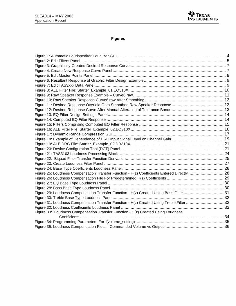
Figures

Figure 1: Automatic Loudspeaker Equalizer GUI .......................................................................................... 4Figure 2: Edit Filters Panel ........................................................................................................................ 5Figure 3: Graphically-Created Desired Response Curve ............................................................................... 7Figure 4: Create New Response Curve Panel .............................................................................................. 7Figure 5: Edit Master Points Panel.............................................................................................................. 8Figure 6: Resultant Response of Graphic Filter Design Example.................................................................... 9Figure 7: Edit TAS3xxx Data Panel............................................................................................................. 9Figure 8: ALE Filter File: Starter_Example_01.EQ310X............................................................................... 10Figure 9: Raw Speaker Response Example – Curve6.raw........................................................................... 11Figure 10: Raw Speaker Response Curve6.raw After Smoothing ................................................................. 12Figure 11: Desired Response Overlaid Onto Smoothed Raw Speaker Response........................................... 12Figure 12: Desired Response Curve After Manual Alteration of Tolerance Bands........................................... 13Figure 13: EQ Filter Design Settings Panel................................................................................................ 14Figure 14: Computed EQ Filter Response ................................................................................................. 14Figure 15: Filters Comprising Computed EQ Filter Response ...................................................................... 15Figure 16: ALE Filter File: Starter_Example_02.EQ310X............................................................................. 16Figure 17: Dynamic Range Compression GUI............................................................................................ 17Figure 18: Example of Dependence of DRC Input Signal Level on Channel Gain ........................................... 19Figure 19: ALE DRC File: Starter_Example_02.DR310X............................................................................. 21Figure 20: Device Configuration Tool (DCT) Panel ..................................................................................... 21Figure 21: TAS3103 Loudness Processing Block ....................................................................................... 24Figure 22: Biquad Filter Transfer Function Derivation................................................................................. 25Figure 23: Create Loudness Filter Panel ................................................................................................... 27Figure 24: Base Type Coefficients Loudness Panel .................................................................................... 28Figure 25: Loudness Compensation Transfer Function - H(z) Coefficients Entered Directly ............................. 28Figure 26: Loudness Compensation File For Predetermined H(z) Coefficients ............................................... 29Figure 27: EQ Base Type Loudness Panel ................................................................................................ 30Figure 28: Bass Base Type Loudness Panel.............................................................................................. 30Figure 29: Loudness Compensation Transfer Function - H(z) Created Using Bass Filter ................................. 31Figure 30: Treble Base Type Loudness Panel............................................................................................ 32Figure 31: Loudness Compensation Transfer Function - H(z) Created Using Treble Filter ............................... 32Figure 32: Loudness Coefficients Loudness Panel ..................................................................................... 33Figure 33: Loudness Compensation Transfer Function - H(z) Created Using Loudness

Coefficients ....................................................................................................................... 34Figure 34: Programming Parameters For f(volume_setting) ......................................................................... 35Figure 35: Loudness Compensation Plots – Commanded Volume vs Output ................................................. 36


Initial Setup Steps

The ALE software package is provided with every TAS3103EVM, and is also available to userswho do not wish to purchase a TAS3103EVM. Requests for the ALE package alone can also be sent [email protected], along with descriptions of the intended end use.

The first step to using the ALE software package is to unzip and install it. Upon opening theinstalled ALE package, the GUI shown in Figure 1 appears. This GUI only applies when using the ALE tocreate equalization (EQ) filter coefficients and is the default GUI. Two other GUIs can be accessed – a GUIfor generating dynamic range compression coefficients and a GUI for generating loudness compensationfilter coefficients.

Figure 1: Automatic Loudspeaker Equalizer GUI

The first step that needs to be taken in using the ALE is to click on the Device button and selectTAS3100. Next, the sample rate of the application being address by ALE needs to be set. This is done byclicking on the View button and selecting Settings. The Frequency Limits tab should come up, but if it doesnot, select it. In the Frequency Limits panel that comes up, the default setting for Fs Sampling FrequencyHz is seen to be 44100 (44.1 KHz). If this is not correct, enter the correct value and click on the OK button.Now the sample rate is properly set.

Create NewDesired ResponseCurve

Replace Section ofCurve Graphically

Copy Master Pointsfrom Curves to EditGrid

Generate Curves fromMaster Points in EditGrid

Draw Filters Stop CalculationLog SampleRaw Curve

Smooth Raw Curve


Filter Coefficient Generation

Manual Filter Generation

To generate a filter, click on the Edit button and select Edit Filter Parameters. The panel shown inFigure 2 results.

Figure 2: Edit Filter Parameters Panel

Butterworth-1HP and Butterworth-1LP are single-pole Butterworth high-pass and low-pass filters.Butterworth-2HP and Butterworth-2LP are two-pole (2nd order) Butterworth high-pass and low-pass filters.High Pass-LR and Low Pass-LR are Linkwitz-Riley high-pass and low-pass filters commonly used in buildingaudio cross-over filters. The programmed cut frequency for these filters is the 6 dB cut frequency ratherthan the standard 3 dB cut frequency. The low plateau filter has 0 dB gain at frequencies above the upperband edge, peaks at the selected gain between the upper and lower band edges, and exhibits a single-poleroll off below the lower band edge. The high plateau filter has 0 dB gain at frequencies below the lowerband edge, peaks at the selected gain between the upper and lower band edges, and exhibits a single-poleroll off above the upper band edge. The low VARi Q and high Vari Q filters are 2nd order low-pass and high-pass filters with selectable peaking at the selected 3-dB frequency. The allpass filter is a second-orderunity-gain filter with a monotonically decreasing phase of 2∏ over the frequency band specified. The EQfilter is a bell-shaped filter with 0 db gain outside the programmed bandwidth, and a peak gain as specifiedwithin the specified bandwidth. The notch filter is a 2nd order notch filter. The treble shelf and bass shelf arestandard 2nd order shelf filters. The cut frequency for treble shelf filters is the 3 dB cut frequency withrespect to the response at frequencies above the cut frequency. The cut frequency for bass shelf filters isthe 3 dB cut frequency with respect to the response at frequencies below the cut frequency. TheChebyshev-1HP and Chebyshev-1LP filters are 2nd order Type-I Chebyshev high-pass and low-pass filters(the 1 in this case references the type Chebyshev filter rather than the order of the filter).

Once a filter type is selected and specified (by clicking on the appropriate tab and entering therequired parameters), clicking on the Draw Filters button generates the filter’s response. If the responsemeets requirements, go to the Edit button and select Generate TAS3xxx Data to generate the biquadcoefficients required to implement the specified response. Going to the Edit button and selecting


Edit TAS3xxx Data displays the values of the generated biquad coefficients, and provides a means ofmanually editing the coefficient file if needed.

Additional filters can be specified and cascaded with filters previously selected and specified byreturning to the Edit Filters panel, selecting another filter type, and entering its parameters. Clicking on theDraw Filters button places the specified filter in cascade with the filters defining the response currentlydisplayed, and generate a new composite response. To save the composite response, go to the Edit buttonand select Generate TAS3xxx Data. To add more filters, repeat the Edit Filters and Draw Filters sequenceuntil the response required is obtained. If a given filter addition does not produce the response desired, itcan be eliminated by going to the Edit Filters panel, highlighting the filter to be eliminated, clicking the rightbutton on the mouse, and clicking on OK in the Confirm Filter Deletion panel that appears. To see theresults, having eliminated the filter, click again on the Draw Filters button.

If the displayed response is the response desired, the TAS3103 coefficients implementing thisresponse need to be generated and then saved. Clicking on the Edit button and selecting GenerateTAS3xxx Data generates the coefficients. The generated data can then be saved to a file by clicking on theFile button and selecting Save As TAS3xxx Program Data. The file name and directory can be selected, butthe file extension must remain EQ310X. Retaining this extension makes the file compatible with theTAS3103 DAS-DCT 2.0 GUI, and from this GUI, the filter can be downloaded into the TAS3103 chip.

There can be confusion over the differences in the roles of Save As TAS3xxx Program Data”andGenerate TAS3xxx Data. When the ALE is first opened and a filter suite is created, clicking on Save AsTAS3xxx Program Data both generates and saves the filter coefficient set. Ever after, however, theGenerate TAS3xxx Data must be selected before the Save As TAS3xxx Program Data is selected in orderto save the latest changes to a previously generated filter suite or to save a newly generated filter set.

Graphic Filter Generation

ALE also provides the ability to draw a required response, and then derive the filter coefficientsrequired to attain the drawn response. (EQ or bell-shaped filters are used exclusively when deriving filters toimplement drawn responses). To use this feature, it is first necessary to go to the File button and selectOpen Raw Response File. Files with both .txt extensions and .raw extensions can be used to specify theraw response, as long as they have the structure shown below. The Data column is the magnituderesponse in dB at the frequency specified.

Hz Data12.20703, -39.4324424.41406, -39.7469136.62109, -40.1941648.82813, -40.7099461.03516, -41.2616

One use for these files is to input speaker response curves. A previously recorded speakerresponse is input into ALE using Open Raw Response File and selecting the desired raw response. A userthen draws a desired speaker. Having drawn the desired speaker response, the ALE can then becommanded to generate a filter that implements the drawn filter response with respect to the raw responsereference. (The desired response can also be input as a file. This option is discussed in the next section).

To begin the construction of a graphically-specified filter response, a raw response must first beinput. When filters are created to implement the specified drawn response, they are created to provide thespecified response given the selected raw response as the starting point. To illustrate this process, anexample is presented. To start, go to the File button, select Open Raw Response File, and then selectzerodb.txt. This selection results in a 0 db reference response (shown as a straight blue line). Next it isnecessary to draw the filter response desired. To draw a filter response, click on the Create New DesiredResponse Curve button. Place the mouse at the desired start point and draw straight-line segments tocreate the filter response desired. When done, click on the Create New Desired Response Curve button


again. This causes a set of magenta boundary lines to be drawn. These lines define the excursionsallowable in generating the filter response from the desired response drawn. An example of a responsegraphically created is shown in Figure 3, and includes the blue 0 dB raw response curve.

Figure 3: Graphically-Created Desired Response Curve

If a mistake is made in drawing the desired response, clicking on the Create New DesiredResponse Curve button a third time will bring up the window shown in Figure 4. Selecting Yes deletes thedrawn desired response curve.

Figure 4: Create New Response Curve Panel

The graphically created response can also be saved as a desired response file by clicking on theFile button and selecting Save as Desired Response. The file name and directory in which to store the filecan be specified, but it is important to maintain the extension .crv. The use of .crv files is illustrated in thenext section.

Once drawn, transferring the points describing the desired response into the computation gridenables manual refinements to be made to the drawn desired response. This transfer is accomplished byclicking on the Copy Master Points From Curves To Edit Grid button. The panel shown in Figure 5 comesup.


Figure 5: Edit Master Points Panel

This panel shows the frequency and amplitude of the Master or inflection points of the drawnresponse curve. These Master points can be edited manually. For example, the amplitude of point 3 can bechanged from 4.928685 to 9.0. Master points can also be deleted or added. To delete a Master point,simply right-mouse click on the Master point to be deleted and then click on the OK button in the ConfirmMaster Point Deletion panel. Master points can be added by going to the empty row in the Edit MasterPoints panel (the row with the * in the Point column) and typing in the frequency and amplitude of the pointto be added.

Any time a change is manually made to the Master points, the Offset Upper Pts button and theOffset Lower Pts button must be clicked to apply the upper and lower tolerances to the revised set of Masterpoints. The Edit Master Points panel can also be used to manually change the upper and lower range of thetolerance curves. Changing tolerance range values manually is accomplished by entering the revisedtolerance range value and clicking on the appropriate Upper Tolerance Pts and Lower Tolerance Ptsbuttons. The Upper Tolerance Pts and The Lower Tolerance Pts tabs in the Edit Master Points panel, onthe other hand, are used when it is desired to change the tolerance level setting at a given individual Masterpoint.

To observe the effect of any manual adjustments on the drawn response, the Generate Curvesfrom Master Points in Edit Grid button must be activated. To save the adjustments made on the drawnresponse, click on the File button and select Save as Desired Response.

The drawn desired response curve and tolerance curves can also be graphically edited. Tographically edit a drawn response curve or tolerance curve, click on the Replace Section Of CurveGraphically button. Then place the cursor on the section of the curve to be modified and drag the mouse todraw the modified shape. Note that this time the shape drawn follows the path of the mouse, and is notrestricted to straight-line segments. Terminate the curve modification by releasing the mouse at a point onthe response or tolerance curve. The start and stop points of the graphic modification must always be onthe original curve.

Once the response curve and the tolerance curves are as required, clicking on the Calculate buttonand selecting Modified Response generates the filters. (Several EQ filters may be required to attain thedesired response. The Modified Response and Pause selection stops the process after each filter is added,requiring the user to click on the OK button on the Continue Calculation panel that comes up between filtercalculations, to continue the process). While the filters are being derived, the Stop Calculation button – thethird button from the right – becomes red. This is an important feature as the computation process can


require minutes to complete, and the red light is the only indication that the program is computationallyactive. As the filters are being calculated the current modified response curve appears in red and the priormodified response curve appears in yellow. Clicking on the Stop Calculation stops the calculation butretains those filters completed up to the point the program was stopped.

The resultant graphic filter design for the drawn filter response example depicted previously isshown in Figure 6.

Figure 6: Resultant Response of Graphic Filter Design Example

Once a filter is calculated, to derive the biquad coefficients for the resultant response it isnecessary to first click on the Edit button and select Copy Generated Filters to Edit Grid. This results in theautomatically generated filters appearing in the Edit Filters panel, shown in Figure 2. The biquadcoefficients for these filters cannot be generated until the filters reside in the Edit Filters panel. Once in theEdit Filters panel, if no manual modifications are to be made, clicking on the Edit button and selectingGenerate TAS3xxx Data generates the biquad coefficients. The Edit TAS3xxx Data panel shown in Figure 7appears. Application specific data, such as Speaker Model #, Speaker Serial #, etc. can be entered in thispanel, and the biquad coefficients generated can be manually modified by typing in changes.

Figure 7: Edit TAS3xxx Data Panel

Clicking on the File button and selecting Save as TAS3xxx Program Data creates a file containingthe filter coefficients, along with the application specific data. The directory to store the file and


the file name can be selected, but the file extension must remain .EQ310X. The content of the .EQ301X filefor the example illustrated is presented in Figure 8. As seen, this example results in the generation of threebiquad filters, and each filter is labeled by an Q## heading (Q1, Q2, and Q3). When the TAS3103 DCT GUIretrieves this file it discards the top information, replaces the Q## number by a sub-address (x##), anddownloads the coefficients into the specified TAS3103 filter bank.

! NAME: A:\Starter_Example_01.EQ310X! Date : 12/27/02! Speaker Model # : Starter_Guide_Speaker! Speaker Serial # : Starter_Guide_Serial #! Speaker Manufacturer: Starter_Guide_Manufacturer! Sample Rate : 44 K Hz! EQ Description : Starter_Guide_EQr!!!# Filter Parameters!# EQ-1, 5.149749, 2006.389480, 309.887964, No, Yes, 1!# EQ-2, -5.204320, 14088.737454, 13022.071425, No, Yes, 2!# EQ-3, -4.825576, 1575.456844, 22050.000000, No, Yes, 3! Channel Number 1Q100 DF 93 45FF A0 34 E700 8D 07 E6FF 20 6C BB00 52 C3 33

Q2FF ED 5F F900 3D A6 6F00 55 42 5F00 12 A0 07FF ED 17 31

Q3FF 2A 08 13FF AA 08 1300 77 0A BF00 D5 F7 ED00 5E ED 2D

Figure 8: ALE Filter File: Starter_Example_01.EQ310X


Equalization Filter Generation

This section addresses using ALE to create equalization filters. In doing so, many other features ofALE will be described – including logarithmic sampling, sample smoothing, frequency boundarymanipulation, tolerance boundary manipulation,

In the previous example, the Raw Response file zerodb.txt was a 0 db reference response shownas a straight blue line. This choice allowed the drawn response to be the response of the filter generated.Another use of the Raw Response file is to provide a means of generating equalization filters directly fromthe raw response curves of the speakers. To do this, the Raw Response file is the raw response curves ofthe speakers, and the drawn response is the desired speaker response. In this case, ALE creates a suite offilters to transform the speaker response from the raw, unprocessed response to the drawn, or desired,response. And, in addition to being able to specify the desired speaker response by drawing the desiredresponse, the desired speaker response can also be specified by inputting a Desired Response file - a .crvfile.

To illustrate the process, the raw speaker response curve6.raw is imported into ALE by going to theFile button, selecting Open Raw Response File, and clicking on curve6.raw. This curve represents theresponse of the speaker to be equalized, and is shown in Figure 9.

Figure 9: Raw Speaker Response Example – Curve6.raw

The points that comprise curve6.raw are linearly placed in frequency. The first task is to convertthe point placement to a logarithmic grid to improve the efficiency of the ALE computation process. (In manyapplications the improvement in processing time can be significant, and is attained with no compromise inthe quality of the equalization process). To convert the raw response curve to a logarithmic grid, click on theLog Sample Raw Curve button, enter the desired number of logarithmically sampled points (300 is typicallyused), and then click OK.

If ALE has to contend with sharp discontinuities in the Raw Response curve while generating thefilter suite required to deliver the desired response, excessive computation time and an excessive number ofgenerated filters results. To combat this problem, a smoothing function is provided to smooth the shape ofthe raw response curve prior to initiating the computation process. Eliminating the sharp discontinuities inthe raw response curve notably improves calculation time and filter count, but has little effect on the overalleffectiveness of the resulting suite of equalization filters. The smoothing process is applied by simplyclicking on the Smooth Raw Curve button. Figure 10 shows the raw response curve that results after


clicking on the Smooth Raw Curve button four times. Note that the sharp discontinuities have beeneliminated.

Figure 10: Raw Speaker Response Curve6.raw After Smoothing

. Next the desired filter response is imported by going to the File button, selecting Open DesiredResponse File, and, for this example, selecting desired_app_note.crv. [.crv files must be generated withinthe ALE program by drawing and editing (if required) a desired response, and then saving the desiredresponse by going to the File button and selecting Save as Desired Response, being sure to maintain the.crv extension.]

The resulting graphic is shown in Figure 11. The blue graph is the raw response, the black graphthe desired response, and the magenta graphs the tolerance bounds about the desired response.

Figure 11: Desired Response Overlaid Onto Smoothed Raw Speaker Response

As seen, for this example the tolerance bound is ± 3 dB. The computational stress points incalculating filters to bring the raw response to the desired response within a tolerance specified by thetolerance band occur on the steep slopes of the desired response curve. If the tolerance bands can berelieved in these sections of the desired response, both calculation time and generated filter count arereduced. To modify the tolerance bands manually, first click on the Replace Section of Curve Graphicallybutton. Then click on one of the ends of the section of the upper or lower tolerance band to be manuallymodified, and drag the mouse to shape the curve as desired, being sure to complete the dragging of themouse on the tolerance band at the other end of the section being modified. Figure 12 shows the results of


manually modifying the tolerance bands bounding the steep slopes of the desired response curve – whichare the frequency sections 30 to 130 Hz and 18 to 22 KHz.

Figure 12: Desired Response Curve After Manual Alteration of Tolerance Bands

One more modification is made before generating the equalization filters. The equalization processneed not extend down to the default lower frequency bound of 2 Hz, nor up to the upper frequency bound ofFs / 2 (Nyquist frequency). Adjusting the frequency bounds to more reasonable settings further reducescomputation time and filter count. To adjust the frequency bounds, click on the View button and selectSettings. This brings up the panel shown in Figure 13. As seen, the lower frequency bound has been set to50 Hz, and the upper bound has been set to 20 KHz. (Also note that the sampling frequency has been setto 44.1 KHz.). When the desired frequency bounds have been set, the Apply button must be clicked.


Figure 13: EQ Filter Design Settings Panel

Now the filters are ready to be calculated. Click on the Calculate button and select ModifiedResponse. The computed filter response that results is shown in red in the plot of Figure 14. (The yellowplot is the modified response prior to the calculation of the final filter).

Figure 14: Computed EQ Filter Response


This particular example required 11 bell-shaped equalization filters, and these 11 filters are shownin Figure 15.

Figure 15: Filters Comprising Computed EQ Filter Response

A file containing these 11 sets of filter coefficients can be created by:

1. Clicking on the Edit button and selecting Copy Generated Filters to Edit Grid to transfer thegenerated filters to the Edit Grid domain.

2. Clicking on the Edit button and selecting Generate TAS3xxx Data generates the biquad coefficients

3. Clicking on the File button and selecting Save as TAS3xxx Program Data creates a .EQ310X filecontaining the filter coefficients, along with the added application specific data.

The content of the file is shown in Figure 16.


Figure 16: ALE Filter File Starter_Example_02.EQ310X

! NAME: C:\Program Files\Texas Instruments Inc\DAP Config Tool2.0\Starter_Example_02.EQ310X! Date : 2/21/03! Speaker Model # :! Speaker Serial # :! Speaker Manufacturer:! Sample Rate : 44 K Hz! EQ Description :!!!# Filter Parameters!# EQ-1, 9.997519, 5265.459281, 13930.606494, No, Yes, 1!# EQ-2, 11.797349, 344.547785, 2194.327307, No, Yes, 2!# EQ-3, -6.285571, 745.270301, 1432.655445, No, Yes, 3!# EQ-4, 11.882147, 13.814435, 97.755808, No, Yes, 4!# EQ-5, 6.096446, 124.661630, 307.354841, No, Yes, 5!# EQ-6, -7.208300, 608.987920, 5701.820308, No, Yes, 6!# EQ-7, 5.372781, 380.760577, 2985.929232, No, Yes, 7!# EQ-8, -4.855725, 568.281489, 4456.470584, No, Yes, 8!# EQ-9, 5.259423, 79.508570, 818.863435, No, Yes, 9!# EQ-10, 3.996107, 13.110451, 165.030929, No, Yes, 10!# EQ-11, -3.798699, 36.377875, 217.753747, No, Yes, 11! Channel Number 1Q1FF B6 1D 52FF C8 52 6800 CE 28 4700 49 E2 AEFF E9 85 52

Q200 ED C0 F0FF 86 22 5900 88 DC 91FF 12 3F 1000 71 01 16

Q300 E1 ED E1FF 99 47 F400 79 7D 66FF 1E 12 1F00 6D 3A A6

Q400 FF B9 37FF 80 40 6F00 80 5E 4FFF 00 46 C900 7F 61 42

Q500 FD 80 D5FF 82 40 E500 81 25 81FF 02 7F 2B00 7C 99 99

Q600 A0 21 A9FF 97 2D 0500 79 77 2EFF 5F DE 5700 6F 5B CD

Q700 E3 05 99FF 86 C3 1C00 82 E5 23FF 1C FA 6700 76 57 C1

Q800 C0 78 E1FF 90 EF A200 7C 5F A7FF 3F 87 1F00 72 B0 B6

Q900 FC D3 E2FF 81 71 1D00 80 99 95FF 03 2C 1E00 7D F5 4D

QA00 FF B0 C0FF 80 3D 2700 80 11 DCFF 00 4F 4000 7F B0 FC

QB00 FE DA A2FF 81 05 F500 7F D1 99FF 01 25 5E00 7F 28 71


Dynamic Range Compressor (DRC) Coefficient Generation

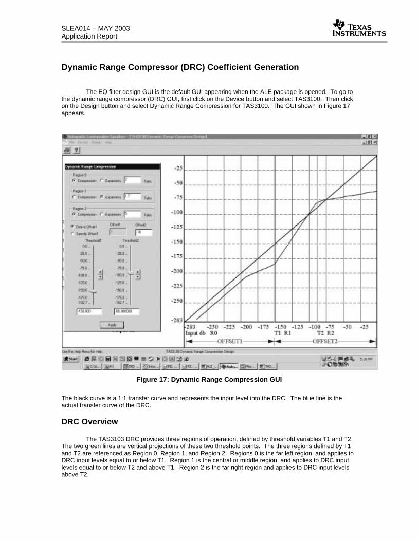
The EQ filter design GUI is the default GUI appearing when the ALE package is opened. To go tothe dynamic range compressor (DRC) GUI, first click on the Device button and select TAS3100. Then clickon the Design button and select Dynamic Range Compression for TAS3100. The GUI shown in Figure 17appears.

Figure 17: Dynamic Range Compression GUI

The black curve is a 1:1 transfer curve and represents the input level into the DRC. The blue line is theactual transfer curve of the DRC.

DRC Overview

The TAS3103 DRC provides three regions of operation, defined by threshold variables T1 and T2.The two green lines are vertical projections of these two threshold points. The three regions defined by T1and T2 are referenced as Region 0, Region 1, and Region 2. Regions 0 is the far left region, and applies toDRC input levels equal to or below T1. Region 1 is the central or middle region, and applies to DRC inputlevels equal to or below T2 and above T1. Region 2 is the far right region and applies to DRC input levelsabove T2.


Within each region, compression (output increases 1 dB for every n dB increase in input) orexpansion (output increases n dB for every 1 dB increase in input) can be specified, and the ratio n isprogrammable. In addition, the offset of the DRC curve from the input curve can be specified at the twothreshold points T1 and T2. The offset of the DRC curve from the input curve at threshold T2 is referred toas Offset2, and the offset of the DRC curve from the input curve at threshold T1 is referred to as Offset1.

DRC Parameter Specification / Computation

There are seven variables that define the operation of the DRC:

• Thresholdso T1o T2

• Compression / Expansion Gainso Region 0o Region 1o Region 2

• Offsetso Offset1o Offset2

The thresholds T1 and T2 define the three regions of DRC operation. Within each region,compression or expansion can be selected, and the degree of compression or expansion within each regioncan be set by inputting the appropriate compression / expansion ratio. Offset1 and Offset2 set the boost orcut of the DRC transfer function at the two threshold points T1 and T2, and serve to place or anchor the gainof the transfer function shape set by T1, T2, and the compression / expansion ratios.

DRC Threshold Settings

The threshold settings can be set either by using the slider associated with each threshold point, orby entering values into the two windows set under the two sliders.

However, the threshold points cannot be set independent of the processing gains programmed intothe TAS3103. The thresholds T1 and T2 are not referenced to the signal level into the TAS3103, but ratherthe signal level into the DRC. To set a threshold point at the DRC input relative to the signal levels into theTAS3103, it is necessary to take the processing gain (or loss) between the TAS3103 input port and theDRC. Assume, as an example, the processing gain structure shown in Figure 18. When the audio signal isinput into the TAS3103, an 8-bit headroom is established above the MSB of the incoming audio data. Inaddition, 8 bits of processing resolution are added below the 32 bits reserved for data input word sizes up to32 bits. The result is a 48-bit word, and this is the word size used in the digital audio processor within theTAS3103. But when the audio data is routed to the DRC, only the upper 32 bits of this 48-bit word are used.This results in a 48 dB attenuation of the signal level into the DRC (8 bits x 6 dB / bit = 48 dB). Channelprocessing gain and use of the dedicated mixer into the DRC can change this apparent 48 dB attenuation insignal level into the DRC. For example, in the figure on the following page, the 24 mixer gain into the DRC,coupled with a net channel gain of 0 dB, changes the net 48 dB attenuation of the signal level into the DRCto a net attenuation of 24 dB. In summary, the ALE set the threshold points for the audio signal levels intothe DRC. Signal levels into the TAS3103, the channel gain with the TAS3103, and the dedicated mixer thatroutes the channel output audio to the DRC must all be comprehended in selecting these threshold settings.


Figure 18: Example of Dependence of DRC Input Signal Level on Channel Gain

DRC Compression / Expansion Settings

Selecting, for each region, either the Compression button or the Expansion button in the DynamicRange Compression panel, makes the choice of compression or expansion for each of the three regions ofthe DRC. The value of the ratio must be equal to or greater than 1.0, with a value of 1.0 giving the DRCtransfer function a slope equal to the slope of the input curve.

For compression, a ratio of n means that the output level changes 1 dB for every n db of change onthe input. For expansion, a ratio of n means that the output level changes by n dB for every 1 dB the inputchanges.

DRC Offset Settings

Entering the value desired (in dB) in the Offset 2 window provided in the Dynamic RangeCompression panel sets Offset2. Offset1 can be entered the same way, using the Offset 1 window, or bycommanding the tool to automatically compute Offset1. Selecting the Derive Offset 1 button or the SpecifyOffset 1 button in the Dynamic Range Compression panel makes this choice.

Threshold T2 serves as the fulcrum or pivot point in the DRC transfer function. There can be nodiscontinuity in the DRC transfer function at T2. This means that the compression and/or expansion plots inregions 1 and 2 must join at threshold T2, and the point of intersection must be offset from the input curve bythe value Offset2. If Offset2 is positive, it is a cut, and the point of intersection is below the input curve bythe value Offset2. If Offset2 is negative, it is a boost, and the point of intersection is above the input curveby the value Offset2.

At input level T1, the compression and/or expansion plots in regions 0 and 1 are not required tointersect. There is a discontinuity in the DRC transfer function at threshold T1 if the transfer curve in region1, which starts at T2 with a value Offset2 relative to the input curve, is not offset from the input curve by avalue Offset1 when the plot intersects the vertical green line projection of T1. To avoid such a discontinuityat T1, Offset1 must be computed knowing the values of T1, T2, Offset2, and the compression / expansioncoefficient k1. To relieve users from having to perform this computation, the ALE GUI provides the option ofnot specifying Offset1 and having the program automatically compute the Offset1 value such that there is no

SAPInputPort

47

4039

87

0

48-BitDAPWord

32

Bit

24

Bit

20

Bit

18Bit

16Bit

Headroom

Resolution

Channel 1Processing

Channel 2Processing

474443

87

0

48-BitDAPWord

24

24

16

DRC

0 dB Gain

0 dB Gain

32

Bit

24

Bit

20

Bit

18Bit

16Bit

Headroom

Resolution


discontinuity at threshold T1. This option is selected by clicking on the Derive Offset1 button on theDynamic Range Compression panel.

Once all the parameters have been entered, clicking on the Apply button enters the data, and theresultant DRC transfer curve is plotted.

DRC Transfer Function Plot

The DRC transfer function for the DRC parameter settings selected can be viewed by clicking onthe Apply button once all parameters have been set. For the ALE GUI window example previously shown,the settings are as follows:

• Thresholdso T1 = -88 dBo T2 = -150.8 dB

• Compression / Expansion Gainso Region 0 = 2:1 Compressiono Region 1 = 1.7:1 Expansiono Region 2 = 5:1 Compression

• Offsetso Offset1 = – 10 dBo Offset2 = Automatically Computed

Unlike the 48-bit word size used in the rest of the digital audio processor, the DRC only uses 32-bitprecision. The LSB then is at –192 dB (32 bits x -6 dB / bit = -192 dB). This means that for levels below -192 dB, the DRC sees a constant input level of 0, and thus the computed DRC gain coefficient remains fixedat the value computed when the input was at -192 dB. This effect is seen in the example DRC plot.

DRC Transfer Function File

Once the desired DRC transfer function is obtained, the result can be saved to a file by clicking onthe File button and selecting Save As DRC2 File. The directory to store the file, and the file name can beselected, but the file extension must remain .DR310X. The content of the .DR301X file for the exampleillustrated is shown in Figure 19. The two threshold values and the two offset values are 48-bit numbers(25.23 format - see Section 3.1.2 in the TAS3103 data manual). The compression / expansion ratios k are28-bit numbers (5.23 format - see Section 3.1.1 in the TAS3103 data manual).


T00 00 00 000C 86 0F 2A00 00 00 0007 4E E8 EF

O00 00 00 0004 D2 00 4A00 00 00 0001 2B 65 80

k0F C0 00 0000 59 99 990F 99 99 9A

Figure 19: ALE DRC File Starter_Example_02.DR310X

The .DR310X extension enables the TAS3103 Device Configuration Tool (DCT) - DAS DCT 2.0GUI – to identify the file as a DRC file. The DCT DRC panel is shown in Figure 20.

Figure 20: Device Configuration Tool (DCT) Panel

As seen, the DRC file created in the ALE tool can be selected in the DCT tool and downloaded to thespecified TAS3103 channel.

{T1}

{T2}

{O1}

{O2}

{k0}{k1}{k2}


In addition to the DRC transfer function, complete specification of the DRC also requires specifyingthe time constants for the energy estimator and the attack and decay filters. The energy estimator derivesan estimate of the rms value of the audio data stream into the DRC. Two programmable parameters, aeand (1 – ae), set the effective time window over which the rms estimate is made in accordance with theequation

( )eAlphaFt

Swindow _1ln

1

−=

The equation only uses (1 Alpha_e) but the GUI requires that both Alpha_e and (1 – Alpaha_e) be entered.

The output of the DRC is a gain coefficient that is used to adjust the level of the audio stream. TheAttack & Decay parameters control the transition time of changes in the computed gain coefficient. Fourparameters define the operation of the Attack & Decay element. Parameters Alpha_d and (1 – Alpha_d) setthe decay or release time constant, and is used when the coefficient change is boosting the volume level.Parameters Alpha_a and (1 – Alpha_a) set the attack time constant, and is used when the coefficientchange is cutting the volume level. The time constants are determined by the equations below, where ta isthe attack time constant and td is the decay time constant.

( )aaFt

Sa −

=1ln

1

( )adFt

Sd −

=1ln

1


Loudness Compensation Filter Design

A listener’s perception of the loudness of a given tone relative to other tones at differentfrequencies is not constant over a range of volume settings. Lower frequency tones are perceived asdropping faster in volume level relative to higher frequency tones as the volume is decreased. This samephenomenon also occurs, to a lesser degree, for higher frequency tones relative to mid-range tones.Typically, loudness compensation involves boosting the bass content, and sometimes the treble content, ofthe audio as the volume is decreased. The TAS3103 provides both a biquad loudness filter to define theportion of the frequency spectrum (bass or treble) to be adjusted in loudness, and four variables thatimplement the function f(volume) that controls the volume adjustment. The ALE TAS3100 loudness filterdesign GUI provides a graphic facility in which to define the parameters of the loudness filter and the fourvariables that define f(volume).

An excellent paper on loudness compensation is Loudness Compensation: Use and Abuse byTomlinson Holman and Frank Kampmann. This article appeared in the Journal of the Audio EngineeringSociety, July / August 1978, Volume 26, Number 7 / 8

Loudness Compensation Transfer Function vs Loudness Biquad FilterTransfer Function

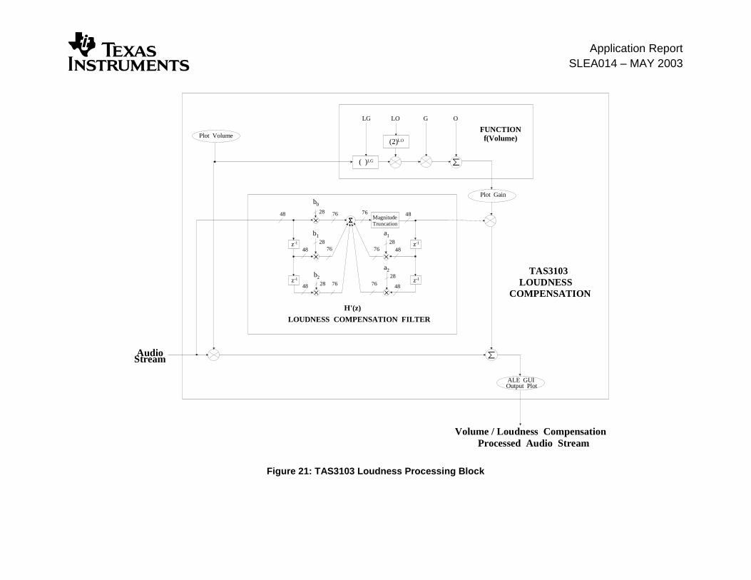
A block diagram of the TAS3100 loudness compensation process is shown in Figure 21. It is notedthat because of the parallel paths that make up the loudness compensation block, the frequency response ofthe loudness biquad filter is not the overall frequency response of the loudness compensation block.Typically, a user wants to specify the frequency response of the loudness compensation block itself, and notworry about the topology of the loudness compensation block. The ALE provides this capability. The ALEalso provides an option for programming the loudness biquad filter directly.

In Figure 21 the composite loudness compensation transfer function can be seen to be

where H’(z) is the transfer function of the biquad loudness filter defining the portion of the spectrum to be

adjusted in volume, is the commanded volume setting, and

is the loudness adjustment coefficient as defined by f(volume). is the same as

f( )).

Plot Volume Plot GainH'(z)Loudness Compensation

Composite Transfer FunctionH(z)

Plot Volume

Plot Volume

Plot Gain

Plot Gain


Figure 21: TAS3103 Loudness Processing Block

AudioStream

( )LG

(2)LO

LG LO G O

z-1

z-1

z-1

z-1

b0

b1

b2

a1

a2

28

28

2828

28

48 76

48

48

48

48

MagnitudeTruncation

48

76

76

76

76

76

H'(z)

LOUDNESS COMPENSATION FILTER

Volume / Loudness CompensationProcessed Audio Stream

Plot Gain

ALE GUIOutput Plot

FUNCTIONf(Volume)Plot Volume

TAS3103LOUDNESS

COMPENSATION


The transfer function of the biquad filter can be derived as shown in Figure 22.

Figure 22: Biquad Filter Transfer Function Derivation

The transfer function H’(z) for the biquad filter can be derived from the biquad equivalent transferfunction of H(z) as follows, assuming

= 1.0 and = 1.0

( ) ( )( ) ( )

( ) ( )( )

( ) ( )( )

( ) ( ) ( )2

21

1

222

1110

1

1'

1'

1'

1'

−−

−−

−−++++−

=

−=−=

−=∴+=

zaza

zabzabbzH

zA

zAzB

zA

zBzH

zHzH

zHzH

To obtain the biquad coefficients for H’(z), the denominator coefficients of the overall loudnessbiquad transfer function H(z) are subtracted from the numerator coefficients of the overall loudness biquadtransfer function H(z) to form the numerator coefficients for the loudness biquad transfer function H’(z). Thedenominator coefficients are the same for both transfer functions.

Using ALE To Specify / Design a Loudness Compensation TransferFunction

The EQ filter design GUI is the default GUI appearing when the ALE package is opened. To go tothe TAS3100 loudness compensation filter design GUI, first click on the Device button and select TAS3100.Then click on the Design button and select Design Loudness Filters For TAS3100. (Note that if the DynamicRange Compressor GUI is present, the Design EQ Filters GUI must first be selected and then the DesignLoudness Filters For TAS3100 GUI selected).

The Loudness Compensation GUI that comes up includes the Create Loudness Filter panel shownin Figure 23. Four options are provided for specifying the Loudness Compensation Transfer Function H(z).

Plot Volume Plot Gain

z-1

z-1

z-1

z-1

b0

b1

b2

a1

a2

Vin(z) Vout(z) = Vin(z) [ b0 + b1z-1 + b2z-2] +

Vout(z) [a1z-1 + a2z

-2]

Vout(z)[1 - a1z-1 - a2z

-2] = Vin(z) [b0 + b1z-1 + b2z

-2]

Vout(z) [b0 + b1z-1 + b2z

-2]= = H'(z)

Vin(z) [1 - a1z-1 - a2z

-2]

BiQuad Filter


1. Enter user-specific biquad coefficients that directly implement H(z)2. Create H(z) using a EQ (bell-shaped) transfer characteristic3. Create H(z) using a bass shelf transfer characteristic4. Create H(z) using a treble shelf transfer characteristic (used if compensation addresses treble)

A fifth option of entering the biquad coefficients for the Loudness Biquad filter H’(z) in the LoudnessCompensation Block is also provided.

Specifying H(z) Using Predetermined Biquad Coefficients

The tab Base Type Coefficients on the Create Loudness Filter panel is used when the equivalentbiquad coefficients for the composite loudness transfer function H(z) have been determined by independentmeans.

To illustrate the use of the Base Type Coefficients tab, click on the Base Type Coefficients tab tobring up the panel shown in Figure 24. For this example, the equivalent biquad coefficients for thecomposite loudness compensation transfer function H(z) are assumed to have been independentlycalculated, assuming a 44.1-kHz sampling frequency, to be:

a1 = 00 FE 2C 33 => 1.985723853a2 = FF 81 CF 93 => -0.9858528375b0 = 00 80 5F 9E => 1.0029180049b1 = FF 01 D3 CD => -1.985723853b2 = 00 7D D0 CF => 0.9829348325

These coefficients have been entered, in decimal, in the coefficient windows provided in the panel. Figure24 indicates which window references which coefficient. Note that it is a requirement that the negativevalues of coefficients a1 and a2 be entered.

Caution: The panel in Figure 24 also implies that the coefficients can be entered as hexadecimalnumbers. This option is not functional, and all work must remain in the decimal domain.However, the ALE correctly outputs the final coefficient values in the hexadecimal formatwhen creating the output file xx.LD310X.

When the coefficients have been entered, clicking on the OK button in the Create Loudness Filterpanel results in a plot of the overall loudness compensation transfer function. This plot is shown in Figure25, and as can be seen, it is nothing more than a bell-shaped EQ filter with the following parameters:

Gain = 3 dBBandwidth = 100 HzCenter Frequency = 80 Hz

Should the full lower frequency range not appear on the plot of Figure 25, it is necessary to go backto the Design EQ Filters GUI by clicking on Design and selecting Design EQ Filters. Then click on File,select Open Raw Response File and open zerodb.txt. This step activates the Automatic LoudspeakerEqualizer GUI. Then click on View, select Settings, click on the Frequency Limits tab, and enter the lowerfrequency limit desired in the LF Lower Frequency Limits Hz window. Then clicking on Design and selectingLoudness Filters for TAS3100l brings back the Loudness filter Design GUI, with the plot now extended downto the lower frequency limit selected. Also, while still in the Automatic Loudspeaker Equalizer GUI, thesampling rate can also be changed by clicking on View, selecting Settings, clicking on the Frequency Limitstab, and entering the desired sampling frequency in Hz in the Fs Sampling Frequency Hz window.


Figure 23: Create Loudness Filter Panel

Create H(z) Directly By Entering TheEquivalent BiQuad Filter Coefficients

Create H(z) Indirectly By Entering The BiQuadCoefficients Of The Loudness BiQuad Filter H'(z)

Use Treble Shelf Filter To Define H(z) Transfer Function

Use EQ (Bell-Shaped) Filter ToDefine H(z) Transfer Function

Use Bass Shelf Filter To DefineH(z) Transfer Function


Figure 24: Base Type Coefficients Loudness Panel

Figure 25: Loudness Compensation Transfer Function - H(z) Coefficients Entered Directly


If it is desired to edit the coefficients for H(z), click on Edit and select Select Filters To EditGraphically. Then click on the generated curve of the transfer function. The Create Loudness Filter panelreappears. Then click on the Base Type Coefficients tab. The entered coefficients reappear and can bealtered as required. Clicking on the OK button results in a second curve being generated. If this secondcurve is the desired response, clicking on Edit, selecting Delete Filters Graphically, and then clicking on thefirst curve generated eliminates the first curve, leaving only the desired response graphed.

When the response desired has been successfully plotted, TAS3103 biquad filter coefficients mustnext be generated. Clicking on Edit, selecting Select Filter to Add to TAS3XXX Data File Graphically, andclicking on the desired response curve accomplishes this. The filter coefficients are now generated.Clicking on File and selecting Save as LD31 Data K… brings up a Save As panel. The file name and foldercan be selected, but the extension LD310X must be retained. This extension allows the TAS3103 GUI torecognize the file as a loudness compensation file. The content of the file generated is shown in Figure 26,with the coefficient identifiers off to the side added for clarity.

Figure 26: Loudness Compensation File For Predetermined H(z) Coefficients

It is noted that the coefficients in Figure 26 are not the same biquad coefficients that were entered for H(z).In fact, the coefficients are the biquad coefficients for H’(z); ALE automatically computes these biquadcoefficients so that they can be directly downloaded into the TAS3103 without requiring any further mappingof coefficients.

Specifying H(z) Using EQ (Bell-Shaped) Filters

H(z) can also be specified by selecting the type filter desired for the composite loudnesscompensation function. Using EQ or bell-shaped filters is one of the options. To use EQ filters to specifyH(z), select the EQ Base Type tab in the Create Loudness Filter panel shown in Figure 23. The panelshown in Figure 27 appears.

To illustrate the use of the panel, enter the filter parameters implemented by the H(z) biquadcoefficients used in the previous example, which are:

Gain in dB = 3 dBBandwidth = 100 HzCenter Frequency = 80 Hz

These parameters are entered by using the appropriate windows of the panel associated with the EQ BaseType selection. Having entered the parameters, clicking on OK plots the H(z) transfer function resultingfrom these gain, bandwidth, and center frequency selections. The plot obtained using the previousparameters is identical to the plot shown in Figure 25.

If the response desired is the response plotted, TAS3103 biquad filter coefficients can begenerated by clicking on Edit, selecting Select Filter to Add to TAS3XXX Data File Graphically, and clickingon the desired response curve. Clicking on File and selecting Save as LD31 Data K… saves the data, oncea file name and directory are entered.

L00 FE 2C 32 => a1 = 1.985723733FF 81 CF 94 => a2 = -0.985852718300 00 5F 9D => b0 = 0.002917885700 00 00 00 => b1 = 0.0FF FF A0 62 => b2 = -0.0029178857


Figure 27: EQ Base Type Loudness Panel

Specifying H(z) Using Bass Shelf Filters

To use Bass Shelf filters to specify H(z), select the Bass Base Type tab in the Create LoudnessFilter panel shown in Figure 23. The panel shown in Figure 28 appears.

Figure 28: Bass Base Type Loudness Panel


The response to the parameters entered in Figure 28 – Bass Gain = 6 dB and Bass Cut (or Boostin this example) Frequency = 150 Hz – is shown in Figure 29.

Figure 29: Loudness Compensation Transfer Function - H(z) Created Using Bass Filter

Clicking on Edit, selecting Select Filter to Add to TAS3XXX Data File Graphically, and clicking onthe desired response curve generates TAS3103 biquad filter coefficients for the Bass Filter response.Clicking on File and selecting Save as LD31 Data K… saves the data, once a file name and directory areentered.

Specifying H(z) Using Treble Shelf Filters

To use Treble Shelf filters to specify H(z), select the Treble Base Type tab in the Create LoudnessFilter panel shown in Figure 23. The panel shown in Figure 30 appears. The response to the parametersentered in Figure 30 – Treble Gain = -4 dB and Bass Cut Frequency = 2000 Hz – is shown in Figure 31.

Clicking on Edit, selecting Select Filter to Add to TAS3XXX Data File Graphically, and clicking onthe desired response curve generates TAS3103 biquad filter coefficients for the Treble Filter response.Clicking on File and selecting Save as LD31 Data K… saves the data, once a file name and directory areentered.


Figure 30: Treble Base Type Loudness Panel

Figure 31: Loudness Compensation Transfer Function - H(z) Created Using Treble Filter


Specifying H’(z) (The Loudness Biquad Filter) Using Predetermined Biquad Coefficients

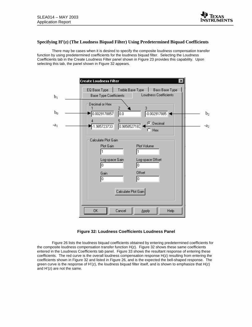
There may be cases when it is desired to specify the composite loudness compensation transferfunction by using predetermined coefficients for the loudness biquad filter. Selecting the LoudnessCoefficients tab in the Create Loudness Filter panel shown in Figure 23 provides this capability. Uponselecting this tab, the panel shown in Figure 32 appears.

Figure 32: Loudness Coefficients Loudness Panel

Figure 26 lists the loudness biquad coefficients obtained by entering predetermined coefficients forthe composite loudness compensation transfer function H(z). Figure 32 shows these same coefficientsentered in the Loudness Coefficients tab panel. Figure 33 shows the resultant response of entering thesecoefficients. The red curve is the overall loudness compensation response H(z) resulting from entering thecoefficients shown in Figure 32 and listed in Figure 26, and is the expected the bell-shaped response. Thegreen curve is the response of H’(z), the loudness biquad filter itself, and is shown to emphasize that H(z)and H’(z) are not the same.

b1

b0 b2

-a1 -a2


Figure 33: Loudness Compensation Transfer Function - H(z) Created Using LoudnessCoefficients

Loudness Compensation vs Volume Command

In addition to specifying the composite loudness transfer function H(z), the programmable loudnessfunction block f(volume_setting) must also be specified to complete a loudness compensation design. Thefiles generated by ALE do not include any of the parameters that govern f(volume_setting), but ALE doesprovide the ability to specify these parameters for display purposes. With this ability, a family of curves forthe filter design chosen can be plotted as a function of volume setting, allowing a user to directly visualizethe loudness compensation achieved for a given loudness filter design.

The output of the function block f(volume_setting) can be expressed in terms of the four I2Cprogrammable loudness compensation coefficients as:

( )[ ] OGsettingvolumesettingvolumef LOLG += *2*_)_(

where:

LG = logarithmic gainLO = logarithmic offsetG = gainO = offset

If LG = 0.5, LO = 0.0, G = 1.0, and O = 0.0, for example, f(volume setting) becomes

Green plot = H’(z)Red plot = H(z)

settingvolumesettingvolumef _)_( =


As noted in Figure 21, the output of f(volume_setting), labeledPlot Gain

in Figure 21, feeds again-control mixer. The output of the loudness biquad filter H’(z) also feeds the same gain-control mixer.The output of this gain-control mixer is then summed with the volume-adjusted audio data stream. The netresult is loudness-adjusted audio. Loudness compensation then allows a given spectral segment of theaudio data stream (as determined by the loudness biquad filter H’(z)) to be given a delta adjustment involume as determined by the programmable function f(volume_setting).

The output of the soft volume / loudness compensation block for the previous example of LG = 0.5,LO = 0.0, G = 1.0, and O = 0.0 is

AudioOut = AudioIn * [volume_setting + H’(z) * settingvolume _ ]

Figure 34 shows the windows for entering LG, LO, G, an O in a given Create Loudness Filter panel.

Figure 34: Programming Parameters For f(volume_setting)

The Plot Volume window is used to enter the commanded volume setting. The Plot Gain window isthe output of the function f(volume_setting). Performance plots are created by entering the commandedvolume setting in the Plot Volume window and clicking on the Apply button. The computed value off(volume_setting) can be seen in the Plot Gain window by clicking on the Calculate Plot Gain window.

Some loudness compensation schemes apply a fixed loudness adjustment coefficient to a range ofvolume settings. In this application, when the volume setting crosses a volume range boundary, a controllerissues a new fixed loudness adjustment coefficient. The TAS3103 and the ALE both support thisimplementation of loudness compensation. In the TAS3103, the computation of f(volume_setting) can beturned off by entering a value of 0 for G. The loudness adjustment coefficient, for this case, is implementedby writing the value the coefficient to the I2C-parameter O (refer to Figure 21). In the ALE, computation off(volume_setting) can be turned off in the very same way by entering a value of 0 for G. Then entering thedesired fixed loudness adjustment coefficient in O, the desired volume command in Plot Volume, clicking onthe Calculate Plot Gain button, and then clicking on the Apply button yields a resultant plot for the volumecommand and loudness adjustment coefficient entered.

LG

G

LO

O

volume settingf(volume_setting)


Figure 35 shows a suite of plots of volume_setting versus the f(volume_setting) function

settingvolume _ for LG = 0.5, LO = 0.0, G = 1.0, and O = 0.0. It is noted that as the commanded

volume setting decreases in value, the amount of bass boost relative to the rest of the audio spectrumincreases. This phenomenon is the purpose of loudness compensation.

Figure 35: Loudness Compensation Plots – Commanded Volume vs Output

Volume Setting Plot Color4.0 Green2.0 Blue1.0 Red0.5 Orange0.25 Yellow

Volume Setting Plot Color0.125 Neon Pink0.0625 Dark Green0.03125 Light Blue0.015625 Blue Green0.0078125 Violet

IMPORTANT NOTICE

Texas Instruments Incorporated and its subsidiaries (TI) reserve the right to make corrections, modifications,enhancements, improvements, and other changes to its products and services at any time and to discontinueany product or service without notice. Customers should obtain the latest relevant information before placingorders and should verify that such information is current and complete. All products are sold subject to TI’s termsand conditions of sale supplied at the time of order acknowledgment.

TI warrants performance of its hardware products to the specifications applicable at the time of sale inaccordance with TI’s standard warranty. Testing and other quality control techniques are used to the extent TIdeems necessary to support this warranty. Except where mandated by government requirements, testing of allparameters of each product is not necessarily performed.

TI assumes no liability for applications assistance or customer product design. Customers are responsible fortheir products and applications using TI components. To minimize the risks associated with customer productsand applications, customers should provide adequate design and operating safeguards.

TI does not warrant or represent that any license, either express or implied, is granted under any TI patent right,copyright, mask work right, or other TI intellectual property right relating to any combination, machine, or processin which TI products or services are used. Information published by TI regarding third–party products or servicesdoes not constitute a license from TI to use such products or services or a warranty or endorsement thereof.Use of such information may require a license from a third party under the patents or other intellectual propertyof the third party, or a license from TI under the patents or other intellectual property of TI.

Reproduction of information in TI data books or data sheets is permissible only if reproduction is withoutalteration and is accompanied by all associated warranties, conditions, limitations, and notices. Reproductionof this information with alteration is an unfair and deceptive business practice. TI is not responsible or liable forsuch altered documentation.

Resale of TI products or services with statements different from or beyond the parameters stated by TI for thatproduct or service voids all express and any implied warranties for the associated TI product or service andis an unfair and deceptive business practice. TI is not responsible or liable for any such statements.

Mailing Address:

Texas InstrumentsPost Office Box 655303Dallas, Texas 75265

Copyright 2003, Texas Instruments Incorporated

ALE Starter Guide - TI

Documents

Transcript of ALE Starter Guide - TI