Ralf Borndorfer k Martin Grotschel & Andreas Lobel

Alcuin's Transportation Problems and Integer Programming

Abstract The need to solve transportation problems was and still is one of the driving forces behind the development of the mathematical disciplines of graph theory, optimization, and operations research. Transportation problems seem to occur for the first time in the literature in the form of the four "River Crossing Problems" in the book Propositiones ad acuen­dos iuvenes. The Propositiones — the oldest collection of mathematical problems written in Latin — date back to the'8th century A.D. and are attributed to Alcuin of York, one of the leading scholars of his time, a royal advisor to Charlemagne at his Prankish court.

Alcuin's river crossing problems had no impact on the development of mathematics. However, they already display all the characteristics of today's large-scale real transportation problems. Prom our point of view, they could have been the starting point of combinatorics, optimization, and operations research. We show the potential of Alcuin's problems in this respect by investigating his problem 18 about a wolf, a goat and a bunch of cabbages with current mathematical methods. This way, we also provide the reader with a leisurely introduction into the modern theory of integer programming.

AMS Subject Classification (1991): 90CIO, 90-01, 90B06, 01A35 Key Words and Phrases: Transportation Problems, Integer Pro­gramming, Alcuin of York

1 Introduction The book Propositiones ad acuendos iuvenes seems to be the oldest collection of mathematical problems written in Latin. It aims at teaching students some basic skills in logic thinking and problem solving. The collection was probably written at the end of the 8th century A.D. and is attributed to Alcuin, see [13], an Anglo-Saxon monk, born in York in 735, one of the leading scholars of his time, head of the Prankish court school at Aachen and a royal advisor of Charlemagne, see [12]. [18] contains an English translation of Alcuin's pro­blems, [13] the Latin "original" together with a German translation. Both

papers also discuss the history of the problems tracing most of them back to ancient Chinese, Egyptian, Greek etc. sources. There is one notable exception. The four "River Crossing Problems" (No. 17-20) seem to appear for the first time in Alcuin's book. We quote here the Singmaster and Hadley translation:

17. Propositio de tribus fratribus singulas habentzbus sorores — About three friends and their sisters. Three friends each with a sister needed to cross a river. Each one of them coveted the sister of another. At the river they found only a small boat, in which only two of them could cross at a time. How did they cross the river without any of the women being defiled by the men?

18. Propositio de lupo et capra etfasciculo cauli — About a wolf, a goat and a bunch of cabbages. A man had to take a wolf, a goat and a bunch of cabbages across the river. The only boat he could find could only take two of them at a time. But he had been ordered to transfer all of these to the other side in good condition. How could this be done?

19. Propositio de viro et muliere ponderantibus plaustrum — About a very heavy man and woman. A man and woman, each the weight of a cartload, with two children who together weigh as much as a cartload, have to cross a river. They find a boat which can only take one cartload. Make the transfer if you can, without sinking the boat.

20. Propositio de ericiis — About Hedgehogs. The Latin text seems to be defective. It seems to say: "About a male and female hedgehog with two young, having weight, wanting to cross a river."

One can obviously view these problems as transportation problems subject to side constraints. Such problems have — in the centuries to come — played prominent roles in shaping the mathematical disciplines of Discrete Mathe­matics (Combinatorics and Graph Theory), Optimization (Linear and Integer Programming), and Operations Research.

The river crossing problems do not seem to have had any impact on the de­velopment of mathematics. They were merely conceived as recreational math­ematics. Prom today's point of view they could have been the starting point of combinatorics and optimization — as we will point out in this paper. But history took a different line.

The roots of combinatorics seem to lie in counting objects and arranging num­bers such as the construction of magic squares. Counting formulas and magic squares can be found in Hindu and Chinese culture more than two thousand

W

years ago. Surprisingly, almost no literature on combinatorics can be found in classical Western civilization. Substantial progress, in particular in the study of magic squares, was made by Chinese and Islamic scholars in the period from 900 to 1300 A.D. Although there was some transmission of this knowledge to the West it was not until the 17th and 18th century that European mathemati­cians took up the subject seriously. Pascal's work on "his" triangle, otivated by his and Fermat's famous correspondence on games of chance around 1654, Leibniz's Dissertatio de Arte Combinatoria in 1666 and Jakob Iernoulli's pa­per Ars Conjectandi, published posthumous in 1713, mark the beginnings of modern combinatorics; Euler's paper on the bridges of Konigsberg 1736 gave birth to the area of graph theory. Note again that Euler's work was inspired by a (recreational) transportation problem. A detailed account of the history of combinatorics can be found in [3].

Also around the end of the 17th century the foundations of optimization were laid through the calculus of variations. A prominent example of this type is the discovery of the brachystochrone by Jakob I Bernoulli and Euler in 16971. However, modern optimization only took off in the 20th century. Its rapid development was and still is closely connected to the progress in computing technology. The origins of linear programming, probably the most intensively used optimization technique and the most cost-saving mathematical tool, can again be traced back to transportation problems. Independent developments in the Soviet Union by [21] (mathematical methods for the organization and plan­ning of production), for which he received the 1975 Nobel Prize in Economics, and in the United States (logistics for the war in the Pacific in the early 1940s) resulted in a general mathematical theory and powerful algorithmic tools that are able to solve linear programs of extremely large scale (see [10] and [24] for the history).

Transportation problems often have integrality constraints because of the indivisibility of commodities or transportation units and, therefore, they also give rise to the study of combinatorial or integer programs. Problems of this type are the famous travelling salesman problem (see [20] for its history), the assignment and transportation problem (discussed in [19] and [22]), network and multicommodity flow and vehicle routing problems (see, for surveys, [1], [11]). An important early example is the case of the Berlin air lift in 1948/1949, which is extensively discussed in [26].

What has all this to do with Alcuin? The point is that Alcuin's river crossing problems could have been the beginning of all these developments. The aim of our paper is to show the potential of his problems in this respect and — in

UMMM

•mm

1 The brachystochrone problem, was also solved by Jakob's younger brother Johann I, who posed the problem to the "deeper thinking mathematicians" of his time in 1696, Euler, de l'Hopital, and Leibniz, but Jakob Bernoulli's and Euler's methods led to the invention of the calculus of variations.

this way — to provide the reader with a leisurely introduction into the modern theory of integer programming and its algorithmic techniques.

2 Alcuin's Solution of his Transportation Prob­lems

Alcuin did not develop general solution procedures for his problems. He simply stated his solution. For problem 18,it reads-.

"I would take the goat and leave the wolf and the cabbage. Then I would return and take the wolf across. Having put the wolf on the other side I would take the goat back over. Having left that behind, I would take the cabbage across. I would then row across again, and having picked up the goat take it over once more. By this procedure there would be some healthy rowing, but no lacerating catastrophe."

Figures 1 and 2a give a pictorial description of the solution.

Figure 1: "I would take the goat and leave the wolf and the cabbage." |

We can only guess how Alcuin arrived at his solutions. But it is very likely that a combination of trial and error, enumeration, and the use of logic impli­cations was used —just as schoolchildren confronted with such problems today would do it.

From our modern point of view, no mathematical theory was developed. Problems were solved by ad-hoc methods. This approach was still in use just one hundred years ago, as is pointed out in [28], where a detailed history of problem 17 is given with its generalization to more than three couples and the additional use of an island in the river. Authors describing such variations and generalizations of Alcuin's transportation problems during the last 1200 years often reported wrong solutions. The errors were (and still are, if ad-hoc enumerative reasoning is used) due to the fact that, in general, the number of possibilities grows extremely fast when additional parameters are introduced. Nowadays this phenomenon is called combinatorial explosion. There is no way

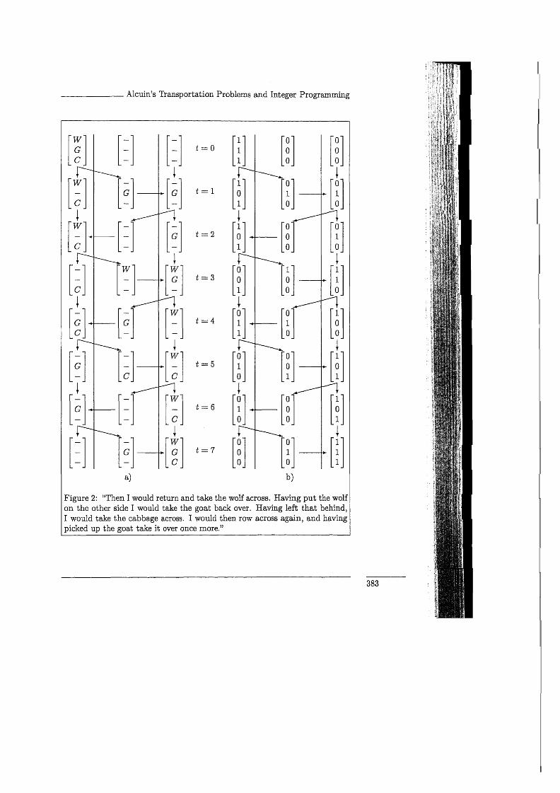
Figure 2: "Then I would return and take the wolf across. Having put the wolf on the other side I would take the goat back over. Having left that behind, I would take the cabbage across. I would then row across again, and having picked up the goat take it over once more."

to avoid it. But today we know reasonable ways to control or structure the "space of solutions'!

3 The Modern Approach Our aim in this paper is to describe a general technique — based on geometry

(polyhedral theory) and linear programming —with which Alcuin's transporta -ton problems and their variants and genera 1'zatons can be matbemafcally modelled and solvecP . In fact, we describe the methodology currently in use

to solve truly large-scale integer programs coming up in practice. We sketch a few of these applications in the final section of this paper .

To show the technique we concentrate on problem 18 about a wolf, a goat, and a bunch of cabbages. It should be clear from our description how the other transportation problems can be handled. We are, of course, aware that problem 18 is quite simple and that we are using a steam hammer to crack a nut. But the technique we describe is very flexible and applies to all kinds of generalizations. The wolf-goat-cabbage problem is not only just a nice ex­ample where the modelling technique can be described easily In fact; quite

surprisingly ,all the mathematical difficulties that arise in integer programming already appear here.

Our starting point is the symbolic description of Alcuin's solution shown in Figures 1 and 2a. We want to transform this description into a representation that admits the use of algebraic and geometric techniques and is suitable for computation.

We indicated the presence of a wolf, goat, or cabbage by writing W, G, or C and the absence by '-'. Instead of W, G, and C, we could also write 1 and instead of '- ' write 0. To remember whether 1 stands for W, G, or C we (arbitrarily) fix an order of the symbols. We agree that symbols always appear

in triples, the first symbol in the triple referring to the wolf, the second to the goat, and the third to the cabbage. For example, with this convention the "old" triple (W, - , C) now reads (1,0,1). Applying this procedure to Figure 2a yields Figure 2b. The advantage of this representation is that we can now "compute with wolves, goats, and cabbages" using standard algebra without introducing special rules for this particular case.

The procedure that we have just applied is a special case of a more general method to bring vector spaces into play. This technique is the following: We assume that we have a (finite) set Nofn elements. We (arbitrarily) number the

2 Our approach is by no means the only modern mathematical method suitable to attack Alcuin's transportation problems. For instance, [4] suggest in exercise 1.8.4 to solve problem 18 as a shortest path problem in a certain state-time graph. This approach is simpler than ours, but it illustrates other techniques than the ones we want to discuss and is not as general.

elements 1, ..., n and define a vector x — Otii • ■ • tXn) where the components are indexed by the elements of N. If M is a subset of N we can represent M by an n-component vector

where

The vector xM is called the characteristic or incidence vector of the subset M of N. In our case of problem 18 the set N consists of the wolf, the goat, and the cabbage. The wolf is the first element and thus represented by the number 1, the goat gets number 2, and the cabbage 3. This way N = {1,2,3} is a representation of the wolf, the goat, and the cabbage and, therefore, every 0/1-vector xM with three components can be viewed as the incidence vector of a "wolf-goat-cabbage configuration" M.

There are several ways (and it is not completely straightforward) how to model the full problem 18 using this technique. We describe one version that is somewhat redundant but conceptionally clear.

Our approach is to view a solution of problem 18 as a sequence of states at different points in time. Let us begin at time t = 0 (again this is just a convention). We introduce three vectors

with the following meaning: x(Q) represents the incidence vector of the wolf-goat-cabbage configuration on one side (we call it the left-hand side) of the river, y(0) the incidence vector of the wolf-goat-cabbage configuration in the boat, and z(0) the incidence vector on the other side (the right-hand side) of the river, all at time t = 0. The initial configuration (the state at time t = 0) in problem 18 is

(1)

(Clearly, our approach could handle any other initial state.) Now we have to make some conventions to record the transformation of states when items are shipped across the river. Let us denote by

as above, the states on the left bank, the boat and the right bank, respectively, at time t = 0,1,2,.... The states x(t) and z(t) correspond to the wolf-goat-cabbage configuration after the i-th shipment has been completed, while y(t) records the boat configuration for the i-fch sh'ipment. Th'is convert "ion'implies that

(2)

(3)

These equations are algebraic representations of the state transitions. Equa­tion (2) describes the transition when an item is shipped from the right-hand side to the left-hand side, i.e., when t is even, while equation (3) models ship­ments from the left to the right. For instance, consider the transition from the initial state state at (even) time t — 0 with wolf-goat-cabbage configuration x(0),z(0) to the next state with wolf-goat-cabbage configuration x(l),z(l) by using the first shipment y(l) (shipping the goat from the left bank to the right bank). Equation (2) yields:

The relations (2) and (3) are not sufficient because we have to guarantee fea­sibility of the states according to Alcuin's stipulations. Since the man rowing the boat can take only one item at a time, we have to introduce additional inequalities

(4)

We interpret Alcuin's phrase "... transfer . . . in good condition" that certain wolf-goat-cabbage configurations are not allowed. 'Wolf and goat' or 'goat and cabbage' are not permitted on the same side without the man. We can take this into account by adding so-called set constraints to the model. The constraint

which is equivalent to stipulating

(5)

requires that whenever the man is not on the left bank, i.e., t is odd, a confi­guration consisting of all three items, the wolf and the goat, or the goat and the cabbage is not permitted.

The modelling of the constraint for the right bank follows the same principle, but needs one more thought. Our aim is to ship all items from the left to the right, i.e., to reach a configuration z(t) = (1,1,1). Clearly, when z(t) = (1,1,1) is reached for the first time, say at time t0, t0 must be odd because a last item has to be moved by the man from the left to the right. When this happens we consider our problem solved and don't want further shipments to occur, i.e., we wish the states to be x{t) = (0,0,0), y(t) = (0,0,0), and z{t) = (1,1,1) for all t > £Q. Thus, we do not exclude the state z(t) = (1,1,1) from our state space for t even. Therefore, our set constraint for the right bank reads

At this point we have arrived at a proper mathematical model of Alcuin's prob­lem 18 in the following sense. For every set of 0/1-vectors x(t): y(t), z(t) G {0, l } 3 , t = 0,1, 2 , . . . , satisfying the constraints (l)-(6) and z(tQ) = (1,1,1) for some tQ > 0, there is a feasible shipment of the wolf, the goat, and the bunch of cabbages such that all three items arrive on the right bank of the river at time to. Conversely, every solution of Alcuin's problem 18 can be encoded into a set of 0/1-vectors as above.

The formulation above is not finite, just as problem 18 is not, since we could always add a few irrelevant additional shipments producing arbitrarily long sequences. As one can see from his solution, Alcuin was clearly interested in a minimum number of shipments. This brings up the optimization aspect and ways to make the problem finite.

One possibility to introduce a finite time horizon is to count the number L of possible states x(t), t odd, on the left bank and observe that, whenever a certain state x(i), t odd, appears for a second time, say x(s) = x(t), where s < t and s and t are odd, then all shipments in the time interval between s and t were unnecessary. The set constraints (5) imply that there are at most L := 5 different feasible wolf-goat-cabbage configurations for t odd on the left bank, and thus, if a feasible solution exists, there must be one with at most T = 2L - 1 = 2 - 5 - 1 = 9 shipments.

Using this or similar observations we can introduce a finite time horizon T, and therefore Alcuin's problem 18 can be viewed as a finite combinatorial problem. More precisely, by adding the "final state constraint"

z(T) = (1,1,1) (7)

we can conclude that the wolf, the goat, and the cabbage can be shipped from

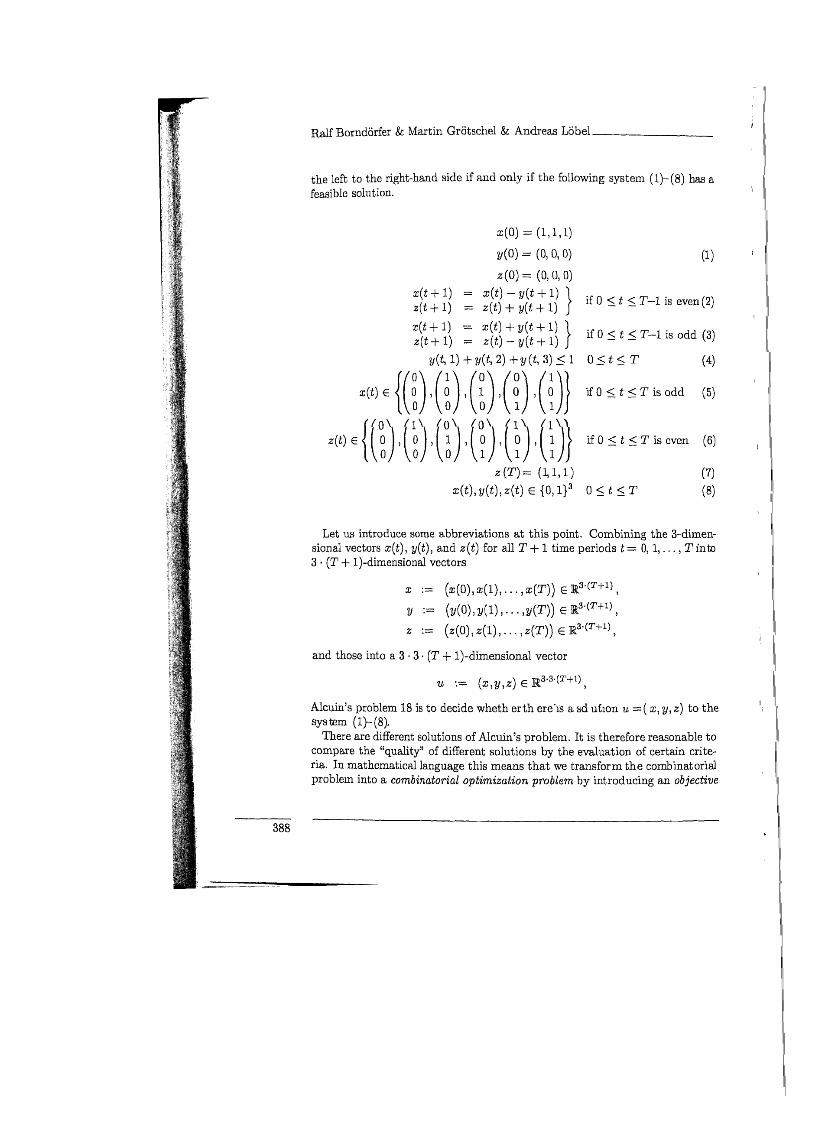
the left to the right-hand side if and only if the following system (l)-(8) has a feasible solution.

(1)

even (2)

odd (3)

(4)

odd (5)

even (6)

(7) (8)

Let us introduce some abbreviations at this point. Combining the 3-dimen-sional vectors x(t), y(t), and z{t) for all T + 1 time periods t = 0, 1 , . . . , T into 3 • (T + l)-dimensional vectors

and those into a 3 • 3 • (T + l)-dimensional vector

Alcuin's problem 18 is to decide wheth erth ere'is a sd ution u=(x,y,z) to the system (l)-(8).

There are different solutions of Alcuin's problem. It is therefore reasonable to compare the "quality" of different solutions by the evaluation of certain crite­ria. In mathematical language this means that we transform the combinatorial problem into a combinatorial optimization problem by introducing an objective

function that evaluates the quality of solutions. There are, as usual, many options.

The most natural option is to minimize the number of trips the man has to do. This is probably what Alcuin had in mind. One is therefore tempted to minimize the function

(9)

which, unfortunately, does not do the job. Namely, this function just counts the loaded trips since, whenever the man crosses the river with one item (the boat carries at most one) at time t, exactly one of the three variables y(t, 1), y[t,2) and y(i,3) is equal to one while the others are zero. But this function does not count the unloaded trips. Thus, unloaded trips can be "added" to any optimum solution without affecting optimality.

A typical "trick" in optimization, with which such situations can be handled, is scaling. We replace the objective function 9, which has only 0/1-coefRcients, by

(10)

For any feasible solution (x,y,z) of (l)-(8), set

i.e., t n i a x is the time of the last nonempty shipment. Now suppose that (x,y, z) and {x',y',z') are two feasible solutions of (l)-(8) with tQ = tmax(x,y,z) < t'Q = tmax(x',y',z'). Then the choice of the scaling factors implies that

Hence if (x,y,z) is a feasible solution of (l)-(8) achieving a minimum value with respect to the objective function (10) then t^^x^y^z) is the minimum number of trips necessary to take the wolf, the goat, and the bunch of cabbages across.

There are other "tricks" to count the number of trips. We could introduce auxiliary "counting variables" that are one as long as the river is crossed. In our case we would define 0/1-variables w{t) for t = 1 , . . . , T satisfying

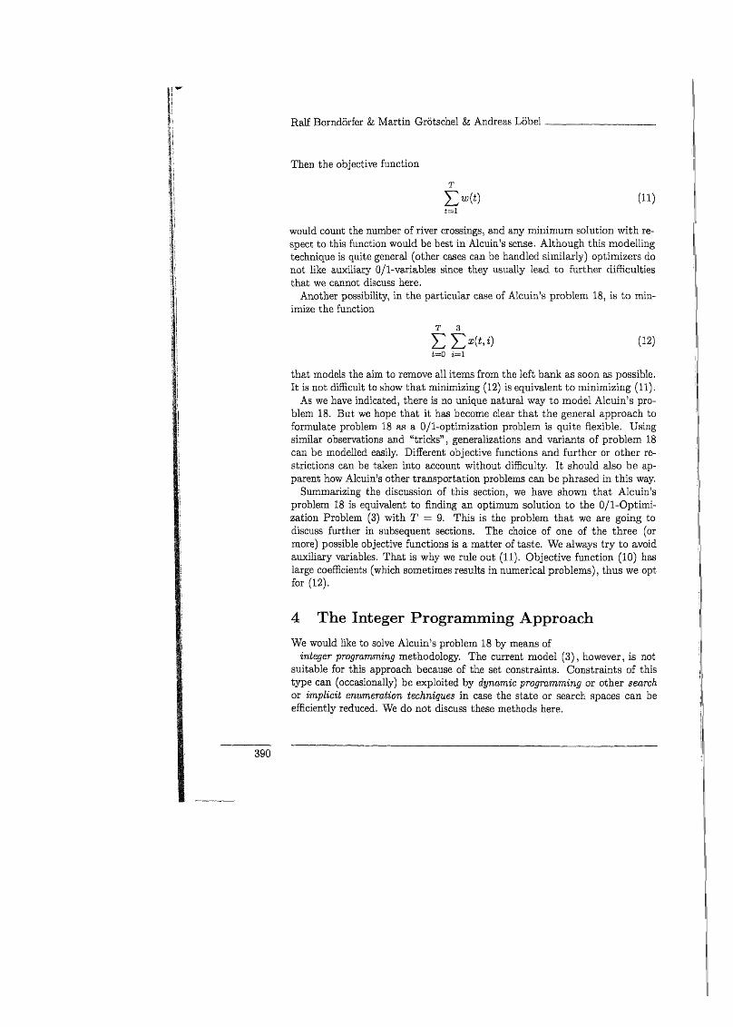
Then the objective function

(11)

would count the number of river crossings, and any minimum solution with re­spect to this function would be best in Alcuin's sense. Although this modelling technique is quite general (other cases can be handled similarly) optimizers do not like auxiliary 0/1-variables since they usually lead to further difficulties that we cannot discuss here.

Another possibility, in the particular case of Alcuin's problem 18, is to min­imize the function

(12)

that models the aim to remove all items from the left bank as soon as possible. It is not difficult to show that minimizing (12) is equivalent to minimizing (11).

As we have indicated, there is no unique natural way to model Alcuin's pro­blem 18. But we hope that it has become clear that the general approach to formulate problem 18 as a 0/1-optimization problem is quite flexible. Using similar observations and "tricks", generalizations and variants of problem 18 can be modelled easily. Different objective functions and further or other re­strictions can be taken into account without difficulty. It should also be ap­parent how Alcuin's other transportation problems can be phrased in this way.

Summarizing the discussion of this section, we have shown that Alcuin's problem 18 is equivalent to finding an optimum solution to the 0/1-Optimi-zation Problem (3) with T = 9. This is the problem that we are going to discuss further in subsequent sections. The choice of one of the three (or more) possible objective functions is a matter of taste. We always try to avoid auxiliary variables. That is why we rule out (11). Objective function (10) has large coefficients (which sometimes results in numerical problems), thus we opt for (12).

4 The Integer Programming Approach We would like to solve Alcuin's problem 18 by means of

integer programming methodology. The current model (3), however, is not suitable for this approach because of the set constraints. Constraints of this type can (occasionally) be exploited by dynamic programming or other search or implicit enumeration techniques in case the state or search spaces can be efficiently reduced. We do not discuss these methods here.

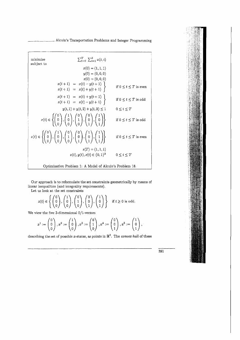
minimize subject to

Optimization Problem 1: A Model of Alcuin's Problem 18.

Our approach is to reformulate the set constraints geometrically by means of linear inequalities (and integrality requirements).

Let us look at the set constraints

We view the five 3-dimensional 0/1-vectors

describing the set of possible z-states, as points in M3. The convex hull of these

points

forms a polytope that we call the x-state polytope. By a general theorem due

Figure 3: z-State Polytope.

to Weyl and Minkowski, see [29], there is, for every finite set V of points in Mn, a finite set of inequalities Ax < b whose solution set is equal to the convex hull of V, and vice versa, for every bounded set P that is the solution set of some inequality system Ax < b, there is a finite set V whose convex hull is equal to P.

So we know that there is a system Ax < b of inequalities with

There are general techniques to determine, given a finite set of points in Mn, an inequality system describing the convex hull of these points (such as Fourier-Motzkin elimination or the double description method, see [26] or [30]). These methods are inherently exponential. In other words, there are examples of a few points that need an enormous number of inequalities for the description of the convex hull.

In our case we are lucky and can easily compute

conv

Similarly, we get a z-state polytope by observing that

conv -

Figure 4: a-State Polytope.

We can use this observation to set up the integer programming problem we are aiming at. We simply replace all the set constraints in Optimization Problem 2 by the corresponding inequality systems. This leads to Optimization Problem 2. One may be tempted to believe that the integrality stipulations are not necessary since we found complete linear descriptions for the individual set constraints. But — as we will see in a minute — this is not so! What we have

Optimization Problem 2: A Integer Program of Alcuin's Problem 18 . I

achieved, however, is the following: Optimization Problem 2 is an integer linear programming model of Alcuin's problem 18, i.e., a description by means of linear constraints and integrality stipulations only. Why is Optimization Problem 2 a better model than the old Optimization Problem 1? The point is that if we delete the integrality constraints from Optimization Problem 2 we obtain an optimization problem over a system of linear equations and inequalities, a so-called linear program, with the property that all feasible integral solutions of this linear program are exactly the solutions of Alcuin's problem 18. This linear program, Optimization Problem 3, is called the LP relaxation of the integer program. The reason for making all these efforts is that there is good commercial and public domain software available that solves linear programs, even of very large size, quite easily.

Does that approach — formulating a problem as an integer linear program

minimize subject to

Optimization Problem 3: The LP Relaxation of Problem 2.

and dropping the integrality constraints — solve Alcuin's problem? Unfortu­nately not! Namely, if we solve the LP Optimization Problem 3, we get the solution shown in Figure 5.

We observe that it is not integral, i.e., the integrality stipulations in (4) were in fact necessary!

Although this is "illegal", we interpret the fractional optimum solution. The interpretation is illustrated in Figure 6. The man first ships the goat (y(l, 2) = 1) from left to right, returns, then ships half the wolf and half the cabbage (y(3,1) = y(3,3) = 0.5) from left to right, returns, and ships the re­maining half of the wolf and the cabbage (y(5,1) = y(5,3) = 0.5) to the right. This "solution" does not violate any of the inequalities of the LP relaxation (4) and requires only 5 shipments, but is certainly not what Alcuin had in mind. The point here is simply that the numbers 0 and 1 are indicating the presence or absence of an item. They are indicator variables and not numeric vari­ables from which we can take fractions. Fractional values of indicator variables

minimize subject to

have no meaning in the "real world" — although we could not withstand the temptation to talk about half a wolf. So, was all this effort just funny nonsense?

Of course not, otherwise we would not have written this paper. As often in mathematics, we go through infeasible domains to arrive at our aim. How we do that will be described in the next sections.

5 The Polyhedral Approach and Cutting Planes

The first attempt to solve the integer programming version (Optimization Prob­lem 2) of Alcuin's problem 18 using only linear programming was not successful. But by extending the idea that we described in Section 4 to reformulate the set constraints we get on the right track. Let us look again at Problem 2.The set of integral vectors

is a solution of Problem 2},

i.e., the set of solutions of Alcuin's problem 18, is finite. Thus the convex hull P of V forms a polytope, and just as for the set constraints (5) and (6), the theorem of Weyl and Minkowski implies the existence of a finite system of inequalities Au < b with

It is well known from polyhedral theory that the set of vertices (extreme points) of P is a subset of V. In fact, since V C {0,1}3-3'(T+1) it is easy to see that V is exactly the set of vertices of P. But Optimization Problem 2 asks for

Figure 6: Half the wolf and the cabbage are shipped over the river . . .

an element of V with minimum objective value, i.e., for a vertex of P with minimum objective value.

Now a simple but fundamental observation of linear programming is the fact that, for any linear objective function cTu, the minimum value of the LP

mincTu = minimize cTu ueP subject to Au < b

is attained at a vertex of P. The famous simplex method exploits exactly this observation. It first finds a vertex of P (in simplex terminology: a basic feasible solution) and then iteratively moves from one vertex to a neighboring vertex with smaller objective function value, until an optimum vertex is reached. Since this vertex is a point in V, our integer program is solved.

To put this approach into practice, we need the system AU < b that descibes P. We have already mentioned that, in general, this system can be very difficult to find. Let's take the travelling sales man problem as an example. There are natural ways to formulate the well known travelling salesman problem as an integer program resulting, for n cities, in travelling salesman polytopes in dimension n(n - l)/2 with \{n - 1)! vertices, see [17]. Table 1 shows for 5 < n < 10 the number of vertices and the number of facets (in equalities necessary to describe the polytope) of the travelling salesman polytope. This table, composed from [9] and [26], gives a glimpse of the enormous growth that may occur here.

Table 1: Combinatorial explosion in the TSP-polytope.

In general, it is practically impossible to compute all the necessary inequali­ties. Even if we could do that it is simply out of question to input them into a computer code and solve the resulting LP. Nevertheless, there are ways to use this approach algorithmically as we will illustrate.

Let us first "do the impossible". Alcuin's problem is still in the range of problem sizes where one can compute all the feasible integer solutions and a complete description of their convex hull by linear inequalities. We did that using the program PORTA ([8]).

Setting the time horizon to T := 9 we obtain an integer program in 3 ■ 3 • (T + 1) = 3 ■ 3 ■ 10 = 90 variables where the first 9 variables are fixed to x(0) = (1,1,1), 2/(0) = (0,0,0), z(Q) = (0,0,0) due to Alcuin's initial condition and where we require 2(9) = (1,1,1), as outlined in the description of our model, as the "terminal state" meaning wolf, goat, and cabbage have to be on the right bank in the end.

We determined all vertices (integral and fractional) of the LP relaxation and took all feasible integral solutions to generate the linear inequalities (facets) and linear equations that are necessary to describe the convex hull of the integral points in R90. The result is displayed in Table 2. All the 20 different integral

Table 2: Complete description of the convex hull.

solutions of Alcuin's problem (for T = 9) and the complete list of 16 inequalities

and 79 equations describing their convex hull can be found in the Appendix in Figures 8 and 9.

The number of equations and inequalities is so small that every commercial LP code solves the resulting LP in a matter of milliseconds. Using the objec­tive function (10) or (12) we obtain exactly the 0/1-representation of Alcuin's solution and have thus succeeded in solving the integer program as a linear program.

In general, however, we don't have the list of all inequalities. In such a case we use what is called the cutting plane approach in combinatorial optimization. This is done as follows.

We first solve the "natural LP relaxation" of the given integer program. In our case, that would be the Optimization Problem 3. If the optimum solution — say u* — is integral we are done (since we are solving an optimization problem over a set larger than the set of integral solutions). If it is not integral (like in our case the solution in Figure 5 happened to be) we search for an inequality or an equality from the complete system describing the convex hull that is violated by the current fractional solution u*. Such an inequality/equation is called a cutting plane, as it cuts off the current solution u*. We modify our present LP by adding the inequality/equation found (of course, in practice we will not only add one cutting plane, but usually as many as we can find - provided that the LP does not get too large) and resolve the LP. We iterate this process until an integral solution is found.

We have done that with Alcuin's problem. The first LP-solution listed in Figure 5 was fractional. This solution does not satisfy the equation (53)

of the complete description listed in Figure 9. In fact, in the LP solution we have

Thus we can use this equation as a cutting plane and add it to the LP. The optimum solution of the new LP was again fractional. We found the new cutting plane

which is inequality (10) from the complete description. We also added this inequality to the LP. The optimum solution of the third LP was integral and again Alcuin's solution.

So with just two additional cutting planes we were able to produce a provably optimum integral solution (by solving three linear programs). This rather sur­prising result is not just a strike of luck. There is a general theory often termed the "polynomial time equivalence of optimization and separation" worked out

in detail in [16] which explains this favorable behavior. Even a short outline of this theory is beyond the scope of this paper.

We did not explain how we determine cutting planes. In Alcuin's case this is easy. Since we have an explicit list of all necessary inequalities and equations, we can simply substitute the fractional solution into the inequalities/equations. As the list is complete and the fractional solution is not in the convex hull of the integral points there must be at least one inequality/equation that is violated and we can use this as a cutting plane. In general, however, this approach requires too much computational effort, even if someone gave us the complete description for free, since the complete systems describing polyhedra associated with combinatorial optimization problems tend to have exponentially many inequalities (see the TSP case already mentioned). That difficulty can be dealt with by means of so-called separation algorithms. The associated theory can be found in [16].

Making this theory practical, i.e., coming up with algorithms that solve prob­lems of the real world efficiently, requires a lot of additional, often problem specific work. We refer the interested reader to [27] for a discussion of the TSP case in this respect.

The same approach also applies when we do not know complete inequality systems describing the convex hull, which, in fact, is the usual case. The cutting plane method is again based on separation algorithms, but these implicitly or explicitly search only parts of the (existing but unknown) complete system. In such a case we may be lucky and find an optimum integral solution (in our case, the initial LP plus only two more inequalities described above would result in such a case), but in general we are not guaranteed to terminate with an integral optimum solution. If that happens, and in practical applications this is usually so, we still have a way out. This is described in the next section.

6 Branch and Bound We have arrived at a state where our LP solver has determined an optimum non-integral solution of our current LP relaxation of the integer program and where our separation algorithms were unable to find a further cutting plane. In Alcuin's problem 18 that could have been after the solution of the initial LP relaxation if we had not been able to compute the inequality system in Figure 9.

At such a point, practice has shown that it is not a bad idea to do something (theoretically) trivial. We resort to (partial) enumeration and combine this with some heuristics.

So let us summarize the current situation. We have a fractional solution of the last LP relaxation at hand. Its objective function value provides by construction a lower bound CL for the (unknown) optimum value copt of the

integer program, i.e.,

Now, in practical applications one usually implements several heuristics that try to find "good" feasible solutions using various problem specific search and improvement techniques. The best such feasible solution provides an upper bound cy for copt .

lower bound copt

optimal solution (unknown)

< cv upper bound

= best known solution

Let us look at the relative error e = Cu~^u (assuming CL > 0). If e = 0 (i.e. cv = CL = copt) we are done. In many applications the data are somewhat "soft" or "fuzzy" and practitioners are perfectly happy with a situation where e = 0.1. That means that we have a feasible solution with value cu that is guaranteed to differ from the optimum value copt by at most 10%.

In Alcuin's case we could use his solution with value cu = Ylx(t,i) = 12 whereas our LP-solution gives a lower bound CL = 9. We are not satisfied with the resulting gap of 331%. That is why we turn to partial enumeration. Using

Figure 7: Branch & Bound searchtree.

some rule (to be determined by problem specific investigation) we choose one of the variables having a fractional value. In our case we choose x(3,l) , i.e., the wolf variable on the left bank in time period three, whose value is 0.5 in our LP solution. In an optimum solution this value must be either 0 or 1. So we create two new subproblems consisting of the old LP plus one of the additional

requirements ar(3,1) = 0 or #(3,1) = 1. This creation of two new subproblems splits the set of feasible integral solutions into two distinct subsets and is called a branching step.

Now we solve each of the resulting new LPs with our LP solver (possibly using the generation of new cutting planes, in which case we call the procedure branch and cut). In each subproblem we get new lower bounds and possibly, running further heuristics, also new upper bounds. If the lower bound at a subproblem is larger than or equal to the best current upper bound we can stop investigating this subproblem since it provably does not contain an integral solution that is better than the current best. This is the bounding or fathoming step with which we can trim the search tree that is generated by iteratively applying the fixing of variables as described above.

The search tree that is obtained in Alcuin's case is shown in Figure 7. We already described how we created two new subproblems from the initial LP relaxation. Solving the LP at subproblem 2 — arising from fixing the wolf variable a;(3,1) to 0 — yields Alcuin's integral solution with objective value 12. We already knew this solution, so our upper bound of 12 is not improved, but since we solved subproblem 2 to (integral) optimality, we can stop processing it. A better solution could, however, still be found in subproblem 3 that we got from the LP relaxation by fixing x(3,1) to 1. Solving this LP yields a fractional solution with value 12. This value is a lower bound on the objective value of all fractional and integral solutions in subproblem 3. But since this objective value equals the value of the best known solution, there cannot be any better integer solution in subproblem 3 and we have fathomed it. So by just examining three subproblems in the searchtree we once more arrived at Alcuin's solution and proved it to be optimal (with respect to objective (12) and thus also with respect to (10)) again.

The search tree could, in principle, consist of 290 nodes turning this approach into (hopelessly ineffective) complete enumeration. In case both the LPs solved on the run and the heuristics provide good bounds on the optimum value the search tree often is of manageable size, as in our case.

This enumerative technique called branch and bound, or implicit enumera­tion, or branch and cut or the like guarantees the finiteness of the procedure that we described - at least theoretically. In Alcuin's case we could easily prove that his solution is optimal.

7 Transportation Problems Alcuin's problems 17,... ,20 are certainly not transportation problems that ap­pear in practical applications. We have chosen problem 18 to show how — in our times — transportation problems are modelled and solved. Surpris­ingly, problem 18 displays all the difficulties in mathematical modelling and

in algorithmically solving real transportation problems of today. In fact, the mathematical techniques and the algorithmic ideas that we sketched in the pre­vious sections are exactly the methods with which large-scale transportation and other combinatorial optimization problems are attacked at present.

It is simply impossible to survey here all the variants of transportation prob­lems that are used in practice and dealt within the mathematics and opera­tions research literature. The Handbook "Network Models" by [Ball, Magnati, Monma and Nemhauser '(1995)] contains several chapters that discuss various types of transportation problems (travelling salesman; watchman routes; as­signment, minimum cost and multicommodity flow problems; path planning), the survey articles [11] and [1] contain broad overviews of the subject and classifications of the problem types. A survey of the field of combinatorial optimization can be found in [15]. The polyhedral methods of integer pro­gramming emphasized in this paper are described in more detail in the articles [17] and [27].

We are currently working on two special and really large-scale logistics prob­lems: Bus scheduling in Hamburg and Berlin and the transportation of disabled persons in Berlin.

The bus scheduling problem is the following. The transportation company of a city has decided (taking many additional requirements and side constraints into account) on a network of lines where buses regularly run. Moreover, the timetable for the bus trips has been determined. The company has several bus depots and types of vehicles. For each trip it is known which vehicle type from which depot can serve it. The task is to assign the vehicles to the trips such that each trip is served by a "legal vehicle" and such that the fleet size is minimized and the cost of the "unloaded trips" (move of a bus without passengers between two trips, or from or to the depot) is as small as possible. This problem can be modelled as a special integral multicommodity flow problem. In case of the city of Berlin, the mathematical model has about 70 million integral variables. We can solve the problem to optimality on fast SUN workstations in about two days of CPU time, see [25].

The city of Berlin operates a fleet of about 100 special buses that can carry 2 to 4 wheel chairs simultaneously. Every disabled person in Berlin is entitled to order rides (under certain side constraints) that will be provided by this system. About 23,000 people currently subscribe to the system and order between 1,000 and 1,500 rides a day on the average. The problem is to schedule the individual rides into buses so that timely service is provided and the overall cost is as small as possible. We have modelled this task, to be solved day by day, as a so-called set partitioning problem, requiring the solution of an integer program

minimize cTx subject to

where A is a 0/1-matrbc with 1,000 to 1,500 rows and 100,000 to 1 million columns and 1 a vector all of whose components are 1. We are unable, at present, to solve this problem to optimality, but we can generate, in a few hours of CPU time, feasible solutions with costs provably at most 10% to 20% above the (unknown) minimum value. A first version of this system started operation in Berlin in June 1995 and resulted in considerable savings (about 25%) compared to the previously used "scheduling by hand", see [5] and [6].

Appendix

Figure 8: List of all integer solutions of Alcuin's problem 18 for T = 9.

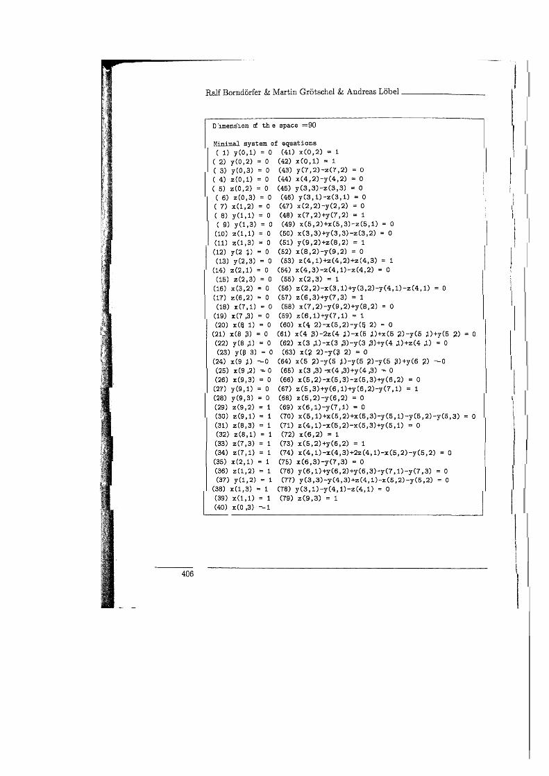
D "intension d th e space =90

Minimal system of equations

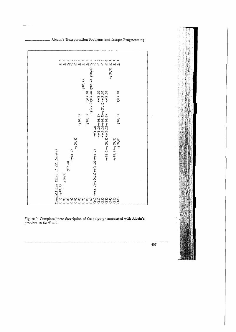
Figure 9: Complete linear description of the polytope associated with Alcuin's problem 18 for T = 9.

References [1] Assad, A., Ball, M., Bodin, L., and Golden, B. (1983). Routing and scheduling

of vehicles and crews. Computers & Operations Research, 10(2):63-211.

[2] Ball, M. 0. , Magnanti, T. L., Monma, C L., and Nemhauser, G. L. (1995). Network Models, Handbooks in Operations Research and Management Science,

volume 7. Elsevier Science B.V., Amsterdam.

[3] Biggs, N. L., Lloyd, E. K., and Wilson, R. J. (1995). The history of combina­torics. In [Graham, Groetschel, Lovasz (1995)], chapter 44.

[4] Bondy, J. A. and Murty, U. S. R. (1976). Graph Theory with Applications. Amer­ican Elsevier, New York, and Macmillan, London.

[5] Borndorfer (1997). Aspects of Set Packing, Partioning, and Covering. Ph D . Thesis. Tech. Univ. Berlin, to appear in 1998.

[6] Borndorfer, Grotschel, Klostermeier, and Kiittner (1997). Berliner Telebus bietet Mobilitat fur Behinderte. Der Nahverkehr 1-2/97, pp. 20-22. 1997.

[7] Butzer ,P .L .and Lohrmann ,D .,editors (1993) .Science in Western and Eastern Civilization in Carolingian Times. Birkhauser Verlag, Basel.

[8] Christof, T. (1994). PORTA - A Polyhedron Representation Transformation Algorithm, version 1.2.1. Written by T. Christof (Univ. Heidelberg), revised by A. Lobel and M. Stoer, available from the ZIB electronic library ELIB via e l ibQzib-ber l in .de , or by anonymous ftp from e l i b . z i b - b e r l i n . d e , in the directory /pub/mathprog/polyth.

[9] Christof, T. and Reinelt, G. (1995). Parallel cutting plane generation for the TSP. In Pritzson, P. and Finmo, L., editors, Parallel Programming and Applica­tions, pages 163-169. IOS Press.

[10] Dantzig, G. B. (1963). Linear Programming and Extensions. Princeton Univer­sity Press, Princeton.

[11] Desrochers, M., Desrosiers, J., and Soumis, F. (1984). Routing with time win­dows by column generation. Networks, 14:545-565.

[12] Fleckenstein, J. (1993). Alcuin im Kreis der Hofgelehrten Karls des Grossen. In [7]-

[13] Folkerts, M. and Gericke, H. (1993). Die Alkuin zugeschriebenen propositiones ad acuendos iuvenes (Aufgaben zur Scharfung des Geistes der Jugend). In [7].

[14] Graham, R., Grotschel, M., and Lovasz, L., editors (1995). Handbook of Combi­natorics, volume 2. Elsevier Science B.V., Amsterdam.

[15] Grotschel, M. and Lovasz, L. (1995). Combinatorial optimization. In [14], chap­ter 28.

[16] Grotschel, M., Lovasz, L., and Schrijver, A. (1988). Geometric algorithms and combinatorial optimization. Springer Verlag, Berlin.

[17] Grotschel, M. and Padberg, M. (1985). Polyhedral theory. In [23], chapter 8.

Hadley, J. and Singmaster, D. (1992). Problems to sharpen the young. The Mathematical Gazette, 76(475): 102-126.

Hitchcock, F. L. (1941). The distribution of a product from several sources to numerous localities. J. Math. Phys., 20:224-230.

Hoffman, A. J. and Wolfe, P. (1985). History. In [23], chapter 1.

Kantorovich, L. (1939). Mathematical Methods in the Organization and Planning of Production. Publication House of the Leningrad State University. Translated in Management Science, Vol. 6, 1960, pp. 366-422.

Koopmans, T. C. (1947). Optimum utilization of the transportation system. In Proceedings of the International Statistical Conferences, Washington D.C. (Vol. 5 reprinted as Supplement to Econometrica, Vol. 17, 1949).

Lawler, E. L., Lenstra, J. K., Rinnooy Kan, A. H. G., and Shmoys, D. B., editors (1985). The Traveling Salesman Problem. John Wiley &c Sons Ltd., Chichester.

Lenstra, J. K., Rinnooy Kan, A. H. G., and Schrijver, A., editors (1991). History of Mathematical Programming. Elsevier Science B.V., Amsterdam.

Lobel (1997). Optimal Vehicle Scheduling in Public Transit. Ph.D. Thesis. Tech. Univ. Berlin, 1997.

Padberg, M. (1995). Linear Optimization and Extensions. Springer Verlag, Berlin.

Padberg, M. and Grotschel, M. (1985). Polyhedral computations. In [23], chap­ter 9.

Pressman, I. and Singmaster, D. (1989). The jealous husbands and The mission­aries and cannibals. The Mathematical Gazette, 73(464) :73-81.

Schrijver, A. (1989). Theory of Linear and Integer Programming. John Wiley &c Sons Ltd., Chichester.

Tschernikow, S. (1971). Lineare Ungleichungen. VEB Deutscher Verlag der Wis-senschaften, Berlin.