aksoy visual grammar - cs.bilkent.edu.tr

October 11, 2002 11:3 Trim Size: 9.75in x 6.5in for Review Volume aksoy˙visual˙grammar

CHAPTER 1

SCENE MODELING AND IMAGE MINING WITH A

VISUAL GRAMMAR

Selim Aksoy, Carsten Tusk, Krzysztof Koperski, Giovanni Marchisio

Insightful Corporation

1700 Westlake Ave. N., Suite 500, Seattle, WA 98109, USA

E-mail: saksoy,ctusk,krisk,[email protected]

Automatic content extraction, classification and content-based retrieval are highlydesired goals in intelligent remote sensing databases. Pixel level processing hasbeen the common choice for both academic and commercial systems. We extendthe modeling of remotely sensed imagery to three levels: Pixel level, region leveland scene level. Pixel level features are generated using unsupervised clustering ofspectral values, texture features and ancillary data like digital elevation models.Region level features include shape information and statistics of pixel level featurevalues. Scene level features include statistics and spatial relationships of regions.This chapter describes our work on developing a probabilistic visual grammarto reduce the gap between low-level features and high-level user semantics, andto support complex query scenarios that consist of many regions with differentfeature characteristics. The visual grammar includes automatic identification ofregion prototypes and modeling of their spatial relationships. The system learnsthe prototype regions in an image collection using unsupervised clustering. Spa-tial relationships are represented by fuzzy membership functions. The systemautomatically selects significant relationships from training data and builds vi-sual grammar models which can also be updated using user relevance feedback. ABayesian framework is used to automatically classify scenes based on these mod-els. We demonstrate our system with query scenarios that cannot be expressedby traditional region or scene level approaches but where the visual grammarprovides accurate classifications and effective retrieval.

1. Introduction

Remotely sensed imagery has become an invaluable tool for scientists, governments,

military, and the general public to understand the world and its surrounding en-

vironment. Automatic content extraction, classification and content-based retrieval

are highly desired goals in intelligent remote sensing databases. Most of the cur-

rent systems use spectral information or texture features as the input for statistical

classifiers that are built using unsupervised or supervised algorithms. The most

commonly used classifiers are the minimum distance classifier and the maximum

likelihood classifier with a Gaussian density assumption. Spectral signatures and

1


2 S. Aksoy et al.

texture features do not always map conceptually similar patterns to nearby lo-

cations in the feature space and limit the success of minimum distance classifiers.

Furthermore, these features do not always have Gaussian distributions so maximum

likelihood classifiers with this assumption fail to model the data. Image retrieval sys-

tems also use spectral or texture features2 to index images and then apply distance

measures3 in these feature spaces to find similarities. However, there is a large se-

mantic gap between the low-level features and the high-level user expectations and

search scenarios.

Pixel level processing has been the common choice for both academic and com-

mercial land cover analysis systems where classifiers have been applied to pixel

level measurements. Even though most of the proposed algorithms use pixel level

information, remote sensing experts use spatial information to interpret the land

cover. Hence, existing systems can only be partial tools for sophisticated analy-

sis of remotely sensed data where a significant amount of expert involvement be-

comes inevitable. This motivated the research on developing algorithms for region-

based analysis with examples including conceptual clustering,38 region growing9

and Markov random field models34 for segmentation of natural scenes; hierar-

chical segmentation for image mining;41 rule-based region classification for flood

monitoring;20 region growing for object level change detection;13 boundary delin-

eation of agricultural fields;32 and task-specific region merging for road extraction

and vegetation area identification.42

Traditional region or scene level image analysis algorithms assume that the re-

gions or scenes consist of uniform pixel feature distributions. However, complex

query scenarios and image scenes of interest usually contain many pixels and regions

that have different feature characteristics. Furthermore, two scenes with similar re-

gions can have very different interpretations if the regions have different spatial

arrangements. Even when pixels and regions can be identified correctly, manual

interpretation is necessary for studies like landing zone and troop movement plan-

ning in military applications and public health and ecological studies in civil ap-

plications. Example scenarios include studies on the effects of climate change and

human intrusion into previously uninhabited tropical areas, and relationships be-

tween vegetation coverage, wetlands and habitats of animals carrying viruses that

cause infectious diseases like malaria, West Nile fever, Ebola hemorrhagic fever and

tuberculosis.12,30 Remote sensing imagery with land cover maps and spatial analysis

is used for identification of risk factors for locations to which infections are likely

to spread. To assist developments in new remote sensing applications, we need a

higher level visual grammar to automatically describe and process these scenarios.

Insightful Corporation’s VisiMine system17,18 supports interactive classifica-

tion and retrieval of remotely sensed images by modeling them on pixel, region and

scene levels. Pixel level characterization provides classification details for each pixel

with regard to its spectral, textural and ancillary (e.g. DEM or other GIS layers)

attributes. Following a segmentation process that computes an approximate poly-


Scene Modeling and Image Mining with a Visual Grammar 3

gon decomposition of each scene, region level features describe properties shared

by groups of pixels. Scene level features describe statistical summaries of pixel and

region level features, and the spatial relationships of the regions composing a scene.

This hierarchical scene modeling bridges the gap between feature extraction and se-

mantic interpretation. VisiMine also provides an interactive environment for train-

ing customized semantic labels from a fusion of visual attributes.

Overviews of different algorithms in VisiMine were presented in our recent

papers.26,25,23,24,19,17,16,18 This chapter describes our work on developing a proba-

bilistic visual grammar4 for scene level image mining. Our approach includes learn-

ing prototypes of primitive regions and their spatial relationships for higher-level

content extraction, and automatic and supervised algorithms for using the visual

grammar for content-based retrieval and classification.

Early work on spatial relationships of regions in image retrieval literature in-

cluded the VisualSEEk project37 where Smith and Chang used representative col-

ors, centroid locations and minimum bounding rectangles to index regions, and

computed similarities between region groups by matching them according to their

colors, absolute and relative locations. Berretti et al.5 used four quadrants of the

Cartesian coordinate system to compute the directional relationship between a pixel

and a region in terms of the number of pixels in the region that were located in

each of the four quadrants around that particular pixel. Then, they extended this

representation to compute the relationship between two regions using a measure of

the number of pairs of pixels in these regions whose displacements fell within each

of the four directional relationships. Centroids and minimum bounding rectangles

are useful when regions have circular or rectangular shapes but regions in natural

scenes often do not follow these assumptions.

Previous work on modeling of spatial relationships in remote sensing applications

utilized the concept of spatial association rules. Spatial association rules15,24 repre-

sent topological relationships between spatial objects, spatial orientation and order-

ing, and distance information. A spatial association rule is of the form X → Y (c%),

where X and Y are sets of spatial or non-spatial predicates and c% is the confidence

of the rule. An example spatial association rule is prevalent endmember(x,concrete)

∧ texture class(x,c1) → close to(x,coastline) (60%). This rule states that 60% of re-

gions where concrete is the prevalent endmember and that texture features belong

to class c1 are close to a coastline. Examples of spatial predicates include topological

relations such as intersect, overlap, disjoint, spatial orientations such as left of and

west of, and distance information such as close to or far away.

Similar work has also been done in the medical imaging area but it usually re-

quires manual delineation of regions by experts. Shyu et al.36 developed a content-

based image retrieval system that used features locally computed from manually

delineated regions. Neal et al.28 developed topology, part-of and spatial associa-

tion networks to symbolically model partitive and spatial adjacency relationships

of anatomical entities. Tang et al.39,40 divided images into small sub-windows, and


4 S. Aksoy et al.

trained neural network classifiers using color and Gabor texture features computed

from these sub-windows and the labels assigned to them by experts. These classi-

fiers were then used to assign labels to sub-windows in unknown images, and the

labels were verified using a knowledge base of label spatial relationships that was

created by experts. Petrakis and Faloutsos29 used attributed relational graphs to

represent features of objects and their relationships in magnetic resonance images.

They assumed that the graphs were already known for each image in the database

and concentrated on developing fast search algorithms. Chu et al.7 described a

knowledge-based semantic image model to represent image objects’ characteristics.

Graph models are powerful representations but are not usable due to the infeasibil-

ity of manual annotation in large databases. Different structures in remote sensing

images have different sizes so fixed sized grids cannot capture all structures either.

Our work differs from other approaches in that recognition of regions and de-

composition of scenes are done automatically, and training of classifiers requires

only a small amount of supervision in terms of example images for classes of in-

terest. The rest of the chapter is organized as follows. An overview of hierarchical

scene modeling is given in Sec. 2. The concept of prototype regions is defined in

Sec. 3. Spatial relationships of these prototype regions are described in Sec. 4. Al-

gorithms for image retrieval and classification using the spatial relationship models

are discussed in Secs. 5 and 6, respectively. Conclusions are given in Sec. 7.

2. Hierarchical Scene Modeling

In VisiMine, we extend the modeling of remotely sensed imagery to three levels:

Pixel level, region level and scene level. Pixel level representations include land cover

labels for individual pixels (e.g. water, soil, concrete, wetland, conifer, hardwood).

Region level representations include shape information and labels for groups of

pixels (e.g. city, residential area, forest, lake, tidal flat, field, desert). Scene level

representations include interactions of different regions (e.g. forest near a water

source, city surrounded by mountains, residential area close to a swamp). This

hierarchical scene representation aims to bridge the gap between data and high-

level semantic interpretation.

The analysis starts from raw data. Then, features are computed to build classi-

fication models for information fusion in terms of structural relationships. Finally,

spatial relationships of these basic structures are computed for higher level model-

ing. Levels of the representation hierarchy are described below.

2.1. Raw Data

The lowest level in the hierarchy is the raw data. This includes multispectral data

and ancillary data like Digital Elevation Models (DEM) or GIS layers. Examples

are given in Figs. 1(a)–1(b).



2.2. Features

Feature extraction is used to achieve a higher level of information abstraction and

summarization above raw data. To enable processing in pixel, region and scene

levels, we use the following state-of-the-art feature extraction methods:

• Pixel level features:

(1) Statistics of multispectral values,

(2) Spectral unmixing for surface reflectance (spectral mixture analysis),25

(3) Gabor wavelet features for microtexture analysis,22

(4) Gray level co-occurrence matrix features for microtexture analysis,10

(5) Laws features for microtexture analysis,21

(6) Elevation, slope and aspect computed from DEM data,

(7) Unsupervised clustering of spectral or texture values.

• Region level features:

(1) Segmentation to find region boundaries (a Bayesian segmentation al-

gorithm under development at Insightful, a hierarchical segmentation

algorithm,41 and a piecewise-polynomial multiscale energy-based re-

gion growing segmentation algorithm14),

(2) Shape information as area, perimeter, centroid, minimum bounding

rectangle, orientation of the principal axis, moments, and roughness

of boundaries,

(3) Statistical summaries (relative percentages) of pixel level features for

each region.

• Scene level features:

(1) Statistical summaries of pixel and region level features for each scene,

(2) Spatial relationships of regions in each scene.

VisiMine provides a flexible tool where new feature extraction algorithms can

be added when new data sources of interest are available. Examples for pixel level

features are given in Figs. 1(c)–1(h). Example region segmentation results are given

in Figs. 2(a) and 2(c).

2.3. Structural Relationships

We use a Bayesian label training algorithm with naive Bayes models35 to perform

fusion of multispectral data, DEM data and the extracted features. The Bayesian

framework provides a probabilistic link between low-level image feature attributes

and high-level user defined semantic structure labels. The naive Bayes model uses

the conditional independence assumption and allows the training of class-conditional

probabilities for each attribute. Training for a particular semantic label is done using

user labeling of pixels or regions as positive or negative examples for that particular

label under training. Then, the probability of a pixel or region belonging to that


6 S. Aksoy et al.

(a) LANDSAT

data

(b) DEM data (c) 15 clusters for

spectral values

(d) 15 clusters for

Gabor features

(e) 15 clusters for

co-occurrence fea-

tures

(f) Spectral mix-

ture analysis

(g) Aspect from

DEM

(h) Slope from

DEM

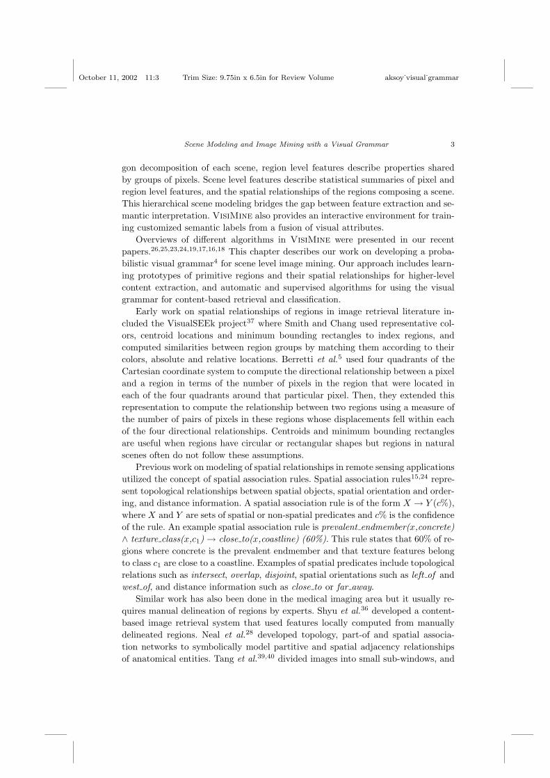
Fig. 1. Raw data and pixel level feature examples for Vancouver, British Columbia. Images in1(c)-1(f) show the cluster labels for each pixel after unsupervised clustering. Images in 1(g)-1(h)

show features computed from DEM data using 3× 3 windows around each pixel. These pixel levelfeatures are used to compute structural relationships for image classification and retrieval.

semantic class is computed as a combination of its attributes using the Bayes rule

(e.g. probability of a region being a residential area given its spectral data, texture

features and DEM data). Figures 2(b) and 2(d) show examples for labels assigned

to regions using the maximum a posteriori probability rule.

2.4. Spatial Relationships

The last level in the hierarchy is scene modeling in terms of the spatial relationships

of regions. Two scenes with similar regions can have very different interpretations if

the regions have different spatial arrangements. Our visual grammar uses region la-

bels identified using supervised and unsupervised classification, and fuzzy modeling

of pairwise spatial relationships to describe high-level user concepts (e.g. border-

ing, invading, surrounding, near, far, right, left, above, below). Fuzzy membership

functions for each relationship are constructed based on measurements like region

perimeters, shape moments and orientations. When the area of interest consists of

multiple regions, the region group is decomposed into region pairs and fuzzy logic



(a)

Bayesian segmen-

tation for Seattle

(b) Region labels

for Seattle

(c)

Bayesian segmen-

tation for Vancou-

ver

(d) Region labels

for Vancouver

Fig. 2. Region level representation examples for Seattle, Washington and Vancouver, British

Columbia. Segmentation boundaries are marked as white. Region labels are city (gray), field (yel-low), green park (lime), residential area (red) and water (blue).

is used to combine the measurements on individual pairs.

Combinations of pairwise relationships enable creation of higher level structures

that cannot be modeled by individual pixels or regions. For example, an airport

consists of buildings, runways and fields around them. An example airport scene

and the automatically recognized region labels are shown in Fig. 3. As discussed

in Sec. 1, other examples include a landing zone scene which may be modeled in

terms of the interactions between flat regions and surrounding hills, public health

studies to find residential areas close to swamp areas, and environmental studies to

find forests near water sources. The rest of the chapter describes the details of the

visual grammar.

(a) LANDSAT

image

(b) Airport

zoomed

(c) Region labels

Fig. 3. Modeling of an airport scene in terms of the interactions of its regions. Region labelsare dry grass (maroon), buildings and runways (gray), field (yellow), residential area (red), water

(blue).


8 S. Aksoy et al.

3. Prototype Regions

The first step to construct a visual grammar is to find meaningful and representa-

tive regions in an image. Automatic extraction of regions is required to handle large

amounts of data. To mimic the identification of regions by experts, we define the

concept of prototype regions. A prototype region is a region that has a relatively

uniform low-level pixel feature distribution and describes a simple scene or part of

a scene. Spectral values or any pixel-level feature listed in Sec. 2.2 can be used for

region segmentation. Ideally, a prototype is frequently found in a specific class of

scenes and differentiates this class of scenes from others. In addition, using proto-

types reduces the possible number of associations between regions and makes the

combinatorial problem of region matching more tractable. (This will be discussed

in detail in Secs. 5 and 6.)

VisiMine uses unsupervised k-means and model-based clustering to automate

the process of finding prototypes. Before unsupervised clustering, image segmen-

tation is used to find regions in images. Interesting prototypes in remote sensing

images can be cities, rivers, lakes, residential areas, tidal flats, forests, fields, snow,

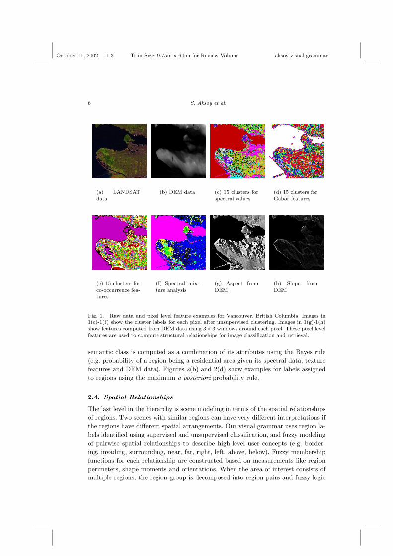
clouds, etc. Figure 4 shows example prototype regions for different LANDSAT im-

ages. The following sections describe the algorithms to find prototype regions in an

image collection.

3.1. K-means Clustering

K-means clustering8 is an unsupervised algorithm that partitions the input sample

into k clusters by iteratively minimizing a squared-error criterion function. Clusters

are represented by the means of the feature vectors associated with each cluster.

In k-means clustering the input parameter k has to be supplied by the user.

Once the training data is partitioned into k groups, the prototypes are represented

by the cluster means. Then, Euclidean distance in the feature space is used to match

regions to prototypes. The degree of match, τij , between region i and prototype j

is computed as

τij =

1 if j = argmint=1,...,k ‖xi − µt‖2

0 otherwise(1)

where xi is the feature vector for region i and µt is the mean vector for cluster t.

3.2. Model-based Clustering

Model-based clustering8 is also an unsupervised algorithm to partition the input

sample. In this case, clusters are represented by parametric density models. Para-

metric density estimation methods assume a specific form for the density function

and the problem reduces to finding the estimates of the parameters of this specific

form. However, the assumed form can be quite different from the true density. On



(a) City (b) Residential

area

(c) Park (d) Lake

(e) Fields (f) Tidal flat (g) Clouds and

shadows

(h) Glacier

Fig. 4. Example prototype regions for different LANDSAT images. Segmentation boundaries are

marked as green and prototype regions are marked as red.

the other hand, non-parametric approaches usually require a large amount of train-

ing data and computations can be quite demanding when the data size increases.

Mixture models can be used to combine the advantages of both parametric and

non-parametric approaches. In a mixture model with k components, the probability

of a feature vector x is defined as

p(x) =

k∑

j=1

αjp(x|j) (2)

where αj is the mixture weight and p(x|j) is the density model for the j’th com-

ponent. Mixture models can be considered as semi-parametric models that are not

necessarily restricted to a particular density form but also have a fixed number of

parameters independent of the size of the data set.

The most commonly used mixture model is the Gaussian mixture with the com-

ponent densities defined as

p(x|j) =1

(2π)q/2|Σj |1/2e−(x−µj)

TΣ−1j

(x−µj)/2 (3)

where µj is the mean vector and Σj is the covariance matrix for the j’th com-


10 S. Aksoy et al.

ponent respectively, and q is the dimension of the feature space, x ∈ Rq. The

Expectation-Maximization (EM) algorithm27 can be used to estimate the param-

eters of a mixture. The EM algorithm first finds the expected value of the data

log-likelihood using the current parameter estimates (expectation step). Then, the

algorithm maximizes this expectation (maximization step). These two steps are re-

peated iteratively. Each iteration is guaranteed to increase the log-likelihood and the

algorithm is guaranteed to converge to a local maximum of the likelihood function.27

The iterations for the EM algorithm proceed by using the current estimates

as the initial estimates for the next iteration. The k-means algorithm can be used

to determine the initial configuration. The mixture weights are computed from

the proportion of examples belonging to each cluster. The means are the cluster

means. The covariance matrices are calculated as the sample covariance of the points

associated with each cluster. Closed form solutions of the EM algorithm for different

covariance structures6,1 are given in Table 1. As a stopping criterion for the EM

algorithm, we can use a threshold for the number of iterations or we can stop if the

change in log-likelihood between two iterations is less than a threshold.

Table 1. Solutions of the Expectation-Maximization algorithm for amixture of k Gaussians. x1, . . . ,xn are training feature vectors inde-

pendent and identically distributed with p(x) as defined in Eq. (2).Covariance structures used are: Σj = σ2

I, all components having the

same spherical covariance matrix; Σj = σ2j I, each component having

an individual spherical covariance matrix; Σj = diag(σ2jt

qt=1), each

component having an individual diagonal covariance matrix; Σj = Σ,each component having the same full covariance matrix; Σj , each

component having an individual full covariance matrix.

Variable Estimate

p(j|xi)αjp(xi|j)

∑

kt=1 αtp(xi|t)

αj

∑ni=1 p(j|xi)

n

µj

∑ni=1 p(j|xi)xi

∑

ni=1 p(j|xi)

Σj = σ2I σ2 =

∑kj=1

∑ni=1 p(j|xi)(xi−µj)T (xi−µj)

nq

Σj = σ2j I σ2

j =∑ni=1 p(j|xi)(xi−µj)T (xi−µj)

q∑

ni=1 p(j|xi)

Σj = diag(σ2jt

qt=1) σ2

jt =

∑ni=1 p(j|xi)(xit−µjt

)2∑

ni=1 p(j|xi)

Σj = Σ Σ =

∑kj=1

∑ni=1 p(j|xi)(xi−µj)(xi−µj)T

n

Σj , full Σj =∑ni=1 p(j|xi)(xi−µj)(xi−µj)T

∑

ni=1 p(j|xi)

The number of components in the mixture can be either supplied by the

user or chosen using optimization criteria like the Minimum Description Length

Principle.31,1 Once the mixture parameters are computed, each component corre-

sponds to a prototype. The degree of match, τij , between region i and prototype j

becomes the posterior probability τij = p(j|xi). The maximum a posteriori proba-



bility (MAP) rule is used to match regions to prototypes where region i is assigned

to prototype j∗ as

j∗ = arg maxj=1,...,k

p(j|xi)

= arg maxj=1,...,k

αjp(xi|j)

= arg maxj=1,...,k

log(αjp(xi|j))

= arg maxj=1,...,k

logαj −1

2log |Σj | −

1

2(xi − µj)

TΣ−1j (xi − µj)

.

(4)

4. Region Relationships

After the regions in the database are clustered into groups of prototype regions,

the next step in the construction of the visual grammar is modeling of their spatial

relationships. The following sections describe how relationships of region pairs and

their combinations can be computed to describe high-level user concepts.

4.1. Second-order Region Relationships

Second-order region relationships consist of the relationships between region pairs.

These pairs can occur in the image in many possible ways. However, the regions of

interest are usually the ones that are close to each other. Representations of spatial

relationships depend on the representations of regions. VisiMine models regions by

their boundary pixels and moments. Other possible representations include mini-

mum bounding rectangles,37 Fourier descriptors33 and graph-based approaches.29

The spatial relationships between all region pairs in an image can be represented

by a region relationship matrix. To find the relationship between a pair of regions

represented by their boundary pixels and moments, we first compute

• perimeter of the first region, πi• perimeter of the second region, πj• common perimeter between two regions, πij• ratio of the common perimeter to the perimeter of the first region, rij =

πijπi

• closest distance between the boundary pixels of the first region and the bound-

ary pixels of the second region, dij• centroid of the first region, νi• centroid of the second region, νj• angle between the horizontal (column) axis and the line joining the centroids,

θij

where i, j ∈ 1, . . . , n and n is the number of regions in the image.

The distance dij is computed using the distance transform.11 Given a particular

region A, to each pixel that is not in A, the distance transform assigns a number

that is the spatial distance between that pixel and A. Then, the distance between


12 S. Aksoy et al.

region A and another region B is the smallest distance transform value for the

boundary pixels of B. The angle θij is computed as

θij =

arccos(

νic−νjcdij

)

if νir ≥ νjr

− arccos(

νic−νjcdij

)

otherwise(5)

where νir and νic are the row and column coordinates of the centroid of region i,

respectively (see Fig. 5 for illustrations). Then, the n×n region relationship matrix

is defined as

R = rij , dij , θij | i, j = 1, . . . , n, ∀i 6= j . (6)

ν1

ν4

θ24

θ31

ν3

θ43

ν2

θ12

c

r

Fig. 5. Orientation of two regions is computed using the angle between the horizontal (column)axis and the line joining their centroids. In the examples above, θij is the angle between the c-axis

and the line directed from the second centroid νj to the first centroid νi. It is used to computethe orientation of region i with respect to region j. θij increases in the clockwise direction, in this

case θ24 < 0 < θ43 < θ31 < θ12.

One way to define the spatial relationships between regions i and j is to use crisp

(Boolean) decisions about rij , dij and θij . Another way is to define them as relation-

ship classes.33 Each region pair can be assigned a degree of their spatial relationship

using fuzzy class membership functions. Denote the class membership functions by

Ωc with c ∈ DIS,BOR, INV,SUR, NEAR,FAR, RIGHT, LEFT,ABOVE,BELOW cor-

responding to disjoined, bordering, invaded by, surrounded by, near, far, right, left,

above and below, respectively. Then, the value Ωc(rij , dij , θij) represents the degree

of membership of regions i and j to class c.

Among the above, disjoined, bordering, invaded by and surrounded by are

perimeter-class relationships, near and far are distance-class relationships, and

right, left, above and below are orientation-class relationships. These relationships

are divided into sub-groups because multiple relationships can be used to describe

a region pair, e.g. invaded by from left, bordering from above, and near and right,

etc. Illustrations are given in Fig. 6.

For the perimeter-class relationships, we use the perimeter ratios rij with the

following trapezoid membership functions:



(a) Perimeter-class relationships: disjoined, bordering, invaded by and surrounded by

(b) Distance-class relationships: near and

far

(c) Orientation-class relationships: right, left, above and below

Fig. 6. Spatial relationships of region pairs.

• disjoined :

ΩDIS(rij) ,

1 if rij = 0

0 otherwise.(7)


14 S. Aksoy et al.

• bordering :

ΩBOR(rij) ,

1 if 0 < rij ≤ 0.40

− 2013rij +

2113 if 0.40 < rij ≤ 1

0 otherwise.

(8)

• invaded by :

ΩINV(rij) ,

10rij − 4 if 0.40 ≤ rij < 0.50

1 if 0.50 ≤ rij ≤ 0.80

− 103 rij +

113 if 0.80 < rij ≤ 1

0 otherwise.

(9)

• surrounded by :

ΩSUR(rij) ,

203 rij −

163 if 0.80 ≤ rij < 0.95

1 if 0.95 ≤ rij ≤ 1

0 otherwise.

(10)

These functions are shown in Fig. 7(a). The motivation for the choice of these

functions is as follows. Two regions are disjoined when they are not touching each

other. They are bordering each other when they have a common perimeter. When

the common perimeter between two regions gets closer to 50%, the larger region

starts invading the smaller one. When the common perimeter goes above 80%, the

relationship is considered an almost complete invasion, i.e. surrounding.

For the distance-class relationships, we use the perimeter ratios rij , distances be-

tween region boundaries dij and sigmoid membership functions with the constraint

ΩNEAR(rij , dij) + ΩFAR(rij , dij) = 1. The membership functions are defined as:

• near :

ΩNEAR(rij , dij) ,

1 if rij > 0e−α(dij−β)

1+e−α(dij−β) otherwise.(11)

• far :

ΩFAR(rij , dij) ,

0 if rij > 01

1+e−α(dij−β) otherwise.(12)

These functions are shown in Fig. 7(b). β is the parameter that determines the

cut-off value when a region becomes more far than near, and α is the parameter

that determines the crispness of the function. We first choose β to be a quarter of

the image width, i.e. β = 0.25w where w is the image width, and then choose α to

give a far fuzzy membership value less than 0.01 at distance 0, i.e. 11+eαβ

< 0.01 ⇒

α > log(99)/β.



Perimeter ratio

Fuz

zy m

embe

rshi

p va

lue

0.0 0.2 0.4 0.6 0.8 1.0

0.0

0.2

0.4

0.6

0.8

1.0

DISJOINEDBORDERINGINVADED_BYSURROUNDED_BY

(a) Perimeter-class spatial relationships

Distance

Fuz

zy m

embe

rshi

p va

lue

0 100 200 300 400 500 600

0.0

0.2

0.4

0.6

0.8

1.0

FARNEAR

(b) Distance-class spatial relationships

Theta

Fuz

zy m

embe

rshi

p va

lue

-4 -3 -2 -1 0 1 2 3 4

0.0

0.2

0.4

0.6

0.8

1.0

RIGHTABOVELEFTBELOW

(c) Orientation-class spatial relationships

Fig. 7. Fuzzy membership functions for pairwise spatial relationships.

For the orientation-class relationships, we use the angles θij and truncated cosine

membership functions with the constraint ΩRIGHT(θij)+ΩLEFT(θij)+ΩABOVE(θij)+

ΩBELOW(θij) = 1. The membership functions are defined as:

• right :

ΩRIGHT(θij) ,

1+cos(2θij)2 if − π/2 < θij < π/2

0 otherwise.(13)

• left :

ΩLEFT(θij) ,

1+cos(2θij)2 if − π < θij < −π/2 or π/2 < θij < π

0 otherwise.(14)


16 S. Aksoy et al.

• above:

ΩABOVE(θij) ,

1−cos(2θij)2 if − π < θij < 0

0 otherwise.(15)

• below :

ΩBELOW(θij) ,

1−cos(2θij)2 if 0 < θij < π

0 otherwise.(16)

These functions are shown in Fig. 7(c).

Note that the pairwise relationships are not always symmetric,

i.e. Ωc(rij , dij , θij) is not necessarily equal to Ωc(rji, dji, θji). Furthermore, some

relationships are stronger than others. For example, surrounded by is stronger than

invaded by, and invaded by is stronger than bordering, e.g. the relationship “small

region invaded by large region” is preferred over the relationship “large region bor-

dering small region”. The class membership functions are chosen so that only one

of them is the largest for a given set of measurements rij , dij , θij . We label a region

pair as having the perimeter-class, distance-class and orientation-class relationships

c1ij = argmaxc∈DIS,BOR,INV,SUR

Ωc(rij , dij , θij)

c2ij = argmaxc∈NEAR,FAR


c3ij = argmaxc∈RIGHT,LEFT,ABOVE,BELOW


(17)

with the corresponding degrees

ρtij = Ωctij(rij , dij , θij), t = 1, 2, 3. (18)

4.2. Higher-order Region Relationships

Higher-order relationships (of region groups) can be decomposed into multiple

second-order relationships (of region pairs). Therefore, the measures defined in the

previous section can be computed for each of the pairwise relationships and can

be combined to measure the combined relationship. The equivalent of the Boolean

“and” operation in fuzzy logic is the “min” operation. For a combination of k re-

gions, there are(

k2

)

= k(k−1)2 pairwise relationships. Therefore, the relationship

between these k regions can be represented as lists of(

k2

)

pairwise relationships

using Eq. (17) as

ct1...k = ctij | i, j = 1, . . . , k, ∀i < j, t = 1, 2, 3 (19)

with the corresponding degrees computed using Eq. (18) as

ρt1...k = mini,j=1,...,k

i<j

ρtij , t = 1, 2, 3. (20)



Example decompositions are given in Fig. 8. These examples show scenarios

that cannot be described by conventional region or scene level image analysis al-

gorithms which assume the regions or scenes consist of pixels with similar feature

characteristics.

5. Image Retrieval

To use the automatically built visual grammar models for image mining, users can

compose queries for complex scene scenarios by giving a set of example regions or

by selecting an area of interest in a scene. VisiMine encodes and searches for a

query scene with multiple regions using the visual grammar as follows:

(1) Let k be the number of regions selected by the user. Find the prototype label

for each of the k regions.

(2) Find the perimeter ratio, distance and orientation for each of the(

k2

)

possible

region pairs.

(3) Find the spatial relationship and its degree for these k regions using Eqs. (19)

and (20). Denote them by ct = ctij | i, j = 1, . . . , k, ∀i < j, t = 1, 2, 3 and

ρt, t = 1, 2, 3, respectively.

(4) For each image in the database,

(a) For each query region, find the list of regions with the same prototype label as

itself. Denote these lists by Ui, i = 1, . . . , k. These regions are the candidate

matches to query regions. Using previously defined prototype labels simplifies

region matching into a table look-up process instead of expensive similarity

computations between region features.

(b) Rank region groups (u1, u2, . . . , uk) ∈ U1 × U2 × · · · × Uk according to the

distance∣

∣

∣

∣

mint=1,2,3

ρt − mint=1,2,3

mini,j=1,...,k

i<j

Ωctij(ruiuj , duiuj , θuiuj )

∣

∣

∣

∣

(21)

or alternatively according to

maxt=1,2,3

maxi,j=1,...,k

i<j

∣

∣

∣ρtij − Ωct

ij(ruiuj , duiuj , θuiuj )

∣

∣

∣. (22)

(c) The equivalent of the Boolean “or” operation in fuzzy logic is the “max”

operation. To rank image tiles, use the distance∣

∣

∣

∣

∣

mint=1,2,3

ρt − max(u1,u2,...,uk)∈U1×U2×···×Uk

mint=1,2,3

mini,j=1,...,k

i<j

Ωctij(ruiuj , duiuj , θuiuj )

∣

∣

∣

∣

∣

(23)

or alternatively the distance

min(u1,u2,...,uk)∈U1×U2×···×Uk

maxt=1,2,3

maxi,j=1,...,k

i<j

∣

∣

∣ρtij − Ωct

ij(ruiuj , duiuj , θuiuj )

∣

∣

∣

. (24)


18 S. Aksoy et al.

Residential area isbordering city

Residential area isbordering water

City is bordering water

Park is surroundedby residential area

LANDSAT image of Seattle

Park is near water

(a) Relationships among residential area, city, park and water in a Seattle scene

LANDSAT image of a forest

Forest is borderingwater of residential area

Forest is to the north Residential area isnear water

(b) Relationships among forest, water and residential area in a forest scene

Buildings and runways arebordering dry grass field bordering dry grass field

Residential area is

LANDSAT image of an airport

Residential area isbordering

buildings and runways

(c) Relationships among buildings, runways, dry grass field and residential area in

an airport scene

Fig. 8. Example decomposition of scenes into relationships of region pairs. Segmentation bound-

aries are marked as white.



In some cases, some of the spatial relationships (e.g. above, right) can be too

restrictive. The visual grammar also includes a DONT CARE relationship class that

allows the user to constrain the searches based on the relationship groups he is

interested in using the VisiMine graphical user interface. Relevance feedback can

also be used to find the most important relationship class (perimeter, distance or

orientation) for a particular query.

Example queries on a LANDSAT database covering Washington State in the

U.S.A. and southern part of British Columbia in Canada are given in Figs. 9–13.

Traditionally, queries that consist of multiple regions are handled by computing a

single set of features using all the pixels in the union of those regions. However,

this averaging causes a significant information loss because features of pixels in

different regions usually correspond to different neighborhoods in the feature space

and averaging distorts the multimodal characteristic of the query. For example,

averaging features computed from the regions in these query scenes ignores the

spatial organization of concrete, soil, grass, trees and water in those scenes. On the

other hand, the visual grammar can capture both feature and spatial characteristics

of region groups.

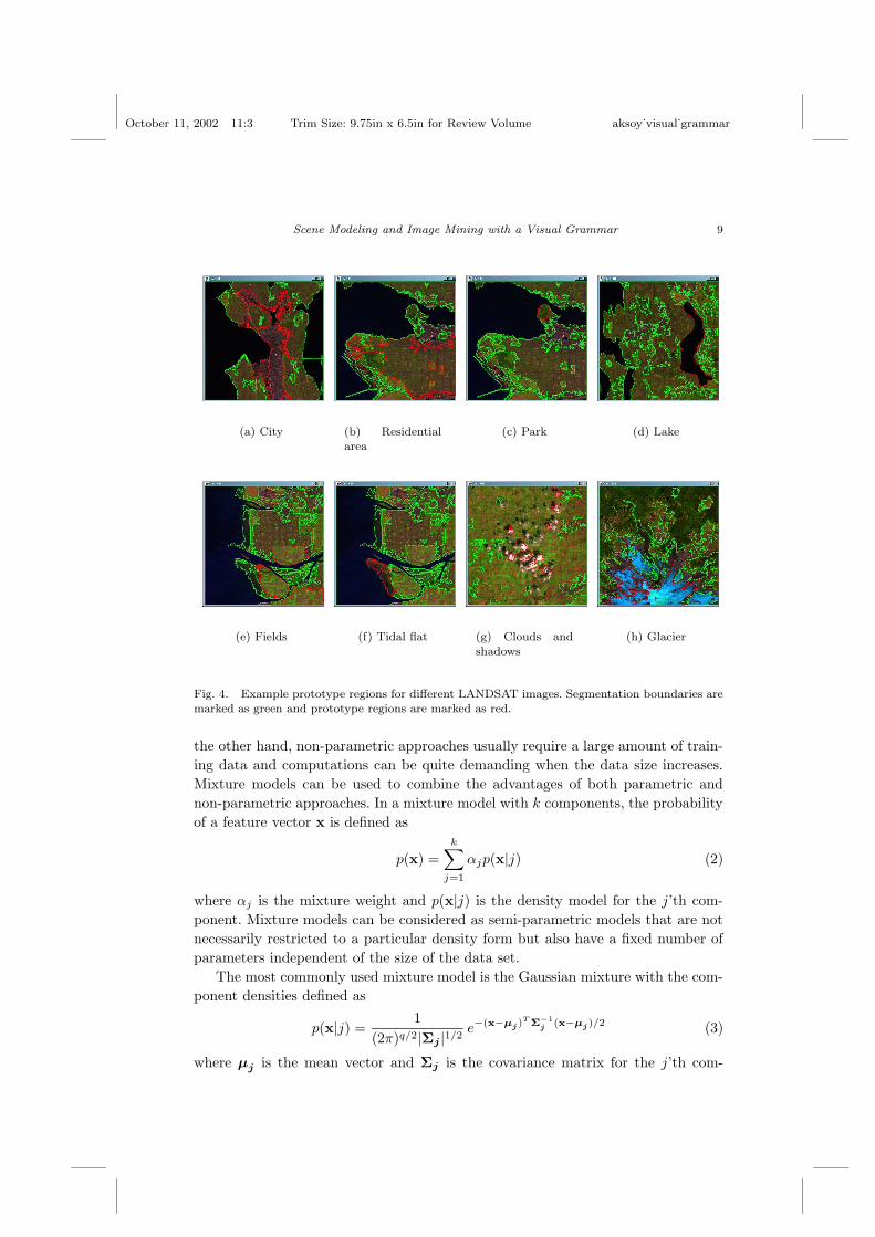
Fig. 9. Search results for a scene where a residential area is bordering a city and both are bordering

water, and a park is surrounded by a residential area and is also near water. Identified regions

are marked by their minimum bounding rectangles. Decomposition of the query scene is given in

Fig. 8(a).

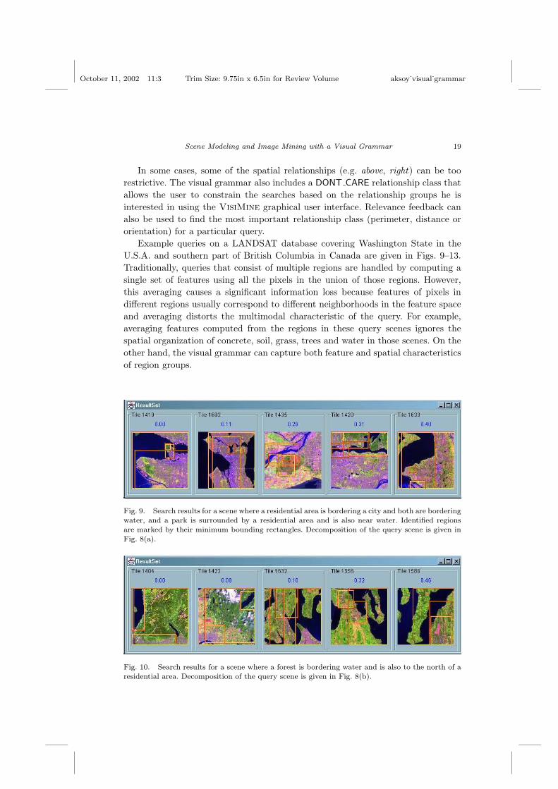
Fig. 10. Search results for a scene where a forest is bordering water and is also to the north of a

residential area. Decomposition of the query scene is given in Fig. 8(b).


20 S. Aksoy et al.

Fig. 11. Search results for a scene where buildings, runways and their neighboring dry grass field

are near a residential area. Decomposition of the query scene is given in Fig. 8(c).

Fig. 12. Search results for a scene where a lake is surrounded by tree covered hills.

Fig. 13. Search results for a scene where a residential area and its neighboring park are both

bordering water.

6. Image Classification

Image classification is defined here as a problem of assigning images to different

classes according to the scenes they contain. Commonly used statistical classifiers

require a lot of training data to effectively compute the spectral and textural signa-

tures for pixels and also cannot do classification based on high-level user concepts

because of the lack of spatial information. Rule-based classifiers also require sig-

nificant amount of user involvement every time a new class is introduced to the



system.

The visual grammar enables creation of higher level classes that cannot be mod-

eled by individual pixels or regions. Furthermore, learning of these classifiers require

only a few training images. We use a Bayesian framework that learns scene classes

based on automatic selection of distinguishing (e.g. frequently occurring, rarely oc-

curring) relations between regions.

The input to the system is a set of training images that contain example scenes

for each class defined by the user. Let s be the number of classes, m be the number

of relationships defined for region pairs, k be the number of regions in a region

group, and t be a threshold for the number of region groups that will be used

in the classifier. Denote the classes by w1, . . . , ws. VisiMine automatically builds

classifiers from the training data as follows:

(1) Count the number of times each possible region group with a particular spa-

tial relationship is found in the set of training images for each class. This is a

combinatorial problem because the total number of region groups (unordered

arrangements without replacement) in an image with n regions is(

nk

)

and the

total number of possible relationships (unordered arrangements with replace-

ment) in a region group is(m+(k2)−1

(k2)

)

. A region group of interest is the one

that is frequently found in a particular class of scenes but rarely exists in other

classes. For each region group, this can be measured using class separability

which can be computed in terms of within-class and between-class variances of

the counts as

ς = log

(

1 +σ2B

σ2W

)

(25)

where σ2W =

∑si=1 vivarzj | j ∈ wi is the within-class variance, vi is the

number of training images for class wi, zj is the number of times this region

group is found in training image j, σ2B = var

∑

j∈wizj | i = 1, . . . , s is the

between-class variance, and var· denotes the variance of a sample.

(2) Select the top t region groups with the largest class separability values. Let

x1, . . . , xt be Bernoulli random variables for these region groups, where xj = T

if the region group xj is found in an image and xj = F otherwise. Let p(xj =

T ) = θj . Then, the number of times xj is found in images from class wi has a

Binomial(vi, θj) =(

vivij

)

θvijj (1 − θj)

vi−vij distribution where vij is the number

of training images for wi that contain xj . The maximum likelihood estimate of

θj becomes

p(xj = T |wi) =vijvi

. (26)

Using a Beta(1, 1) distribution as the conjugate prior, the Bayes estimate for

θj is computed as

p(xj = T |wi) =vij + 1

vi + 2. (27)


22 S. Aksoy et al.

Using a similar procedure with Multinomial and Dirichlet distributions, the

Bayes estimate for an image belonging to class wi (i.e. containing the scene

defined by class wi) is computed as

p(wi) =vi + 1

∑si=1 vi + s

. (28)

In other words, discrete probability tables are constructed using vi and vij ,

i = 1, . . . , s, j = 1, . . . , t, and conjugate priors are used to update them when

new images become available via relevance feedback.

(3) For an unknown image, search for each of the t region groups (determine whether

xj = T or xj = F, ∀j) and compute the probability for each class using the

conditional independence assumption as

p(wi|x1, . . . , xt) =p(wi, x1, . . . , xt)

p(x1, . . . , xt)

=p(wi)p(x1, . . . , xt|wi)

p(x1, . . . , xt)

=p(wi)

∏tj=1 p(xj |wi)

p(x1, . . . , xt).

(29)

Assign that image to the best matching class using the MAP rule as

w∗ = argmaxwi

p(wi|x1, . . . , xt)

= argmaxwi

p(wi)

t∏

j=1

p(xj |wi).(30)

Classification examples are given in Figs. 14–16. We used four training images

for each of the classes defined as “clouds”, “tree covered islands”, “residential areas

with a coastline”, “snow covered mountains”, “fields” and “high-altitude forests”.

These classes provide a challenge where a mixture of spectral, textural, elevation and

spatial information is required for correct identification of the scenes. For example,

pixel level classifiers often misclassify clouds as snow and shadows as water. On the

other hand, the Bayesian classifier described above could successfully eliminate most

of the false alarms by first recognizing regions that belonged to cloud and shadow

prototypes and then verified these region groups according to the fact that clouds

are often accompanied by their shadows in a LANDSAT scene. Other scene classes

like residential areas with a coastline or tree covered islands cannot be identified

by pixel level or scene level algorithms that do not use spatial information. The

visual grammar classifiers automatically learned the distinguishing region groups

that were frequently found in particular classes of scenes but rarely existed in other

classes.



(a) Training images

(b) Images classified as containing clouds

Fig. 14. Classification results for the “clouds” class which is automatically modeled by the dis-tinguishing relationships of white regions (clouds) with their neighboring dark regions (shadows).

7. Conclusions

In this chapter we described a probabilistic visual grammar to automatically an-

alyze complex query scenarios using spatial relationships of regions and described

algorithms to use it for content-based image retrieval and classification. Our hier-

archical scene modeling bridges the gap between feature extraction and semantic

interpretation. The approach includes unsupervised clustering to identify prototype

regions in images (e.g. city, residential, water, field, forest, glacier), fuzzy modeling

of region spatial relationships to describe high-level user concepts (e.g. bordering,

surrounding, near, far, above, below), and Bayesian classifiers to learn image classes


24 S. Aksoy et al.

(a) Training images

(b) Images classified as containing tree covered islands

Fig. 15. Classification results for the “tree covered islands” class which is automatically modeledby the distinguishing relationships of green regions (lands covered with conifer and deciduous

trees) surrounded by blue regions (water).

based on automatic selection of distinguishing (e.g. frequently occurring, rarely oc-

curring) relations between regions.

The visual grammar overcomes the limitations of traditional region or scene

level image analysis algorithms which assume that the regions or scenes consist of

uniform pixel feature distributions. Furthermore, it can distinguish different inter-

pretations of two scenes with similar regions when the regions have different spatial

arrangements. We demonstrated our system with query scenarios that could not be

expressed by traditional pixel, region or scene level approaches but where the visual

grammar provided accurate classification and retrieval.



(a) Training images

(b) Images classified as containing residential areas with a coastline

Fig. 16. Classification results for the “residential areas with a coastline” class which is automati-

cally modeled by the distinguishing relationships of regions containing a mixture of concrete, grass,trees and soil (residential areas) with their neighboring blue regions (water).

Future work includes using supervised methods to learn prototype models in

terms of spectral, textural and ancillary GIS features; new methods for user assis-

tance for updating of visual grammar models; automatic generation of metadata


26 S. Aksoy et al.

for very large databases; and natural language search support (e.g. “Show me an

image that contains a city surrounded by a forest that is close to a water source.”).

Insightful Corporation’s InFact product is a natural language question answering

platform for mining unstructured data. A VisiMine–InFact interface will be an

alternative to the query-by-example paradigm by allowing natural language-based

searches on large remote sensing image archives. This will especially be useful for

users who do not have query examples for particular scenes they are looking for, or

when transfer of large image data is not feasible over slow connections.

Acknowledgments

This work is supported by the NASA contract NAS5-01123 and NIH Phase II grant

2-R44-LM06520-02.

References

1. S. Aksoy. A Probabilistic Similarity Framework for Content-Based Image Retrieval.PhD thesis, University of Washington, Seattle, WA, June 2001.

2. S. Aksoy and R. M. Haralick. Using texture in image similarity and retrieval. InM. Pietikainen, editor, Texture Analysis in Machine Vision, volume 40 of Series inMachine Perception and Artificial Intelligence, pages 129–149. World Scientific, 2000.

3. S. Aksoy and R. M. Haralick. Feature normalization and likelihood-based similaritymeasures for image retrieval. Pattern Recognition Letters, 22(5):563–582, May 2001.

4. S. Aksoy, G. Marchisio, K. Koperski, and C. Tusk. Probabilistic retrieval with a vi-sual grammar. In Proceedings of IEEE International Geoscience and Remote Sensing

Symposium, volume 2, pages 1041–1043, Toronto, Canada, June 2002.5. S. Berretti, A. Del Bimbo, and E. Vicario. Modelling spatial relationships betweencolour clusters. Pattern Analysis & Applications, 4(2/3):83–92, 2001.

6. G. Celeux and G. Govaert. Gaussian parsimonious clustering models. Pattern Recog-

nition, 28:781–793, 1995.7. W. W. Chu, C.-C. Hsu, A. F. Cardenas, and R. K. Taira. Knowledge-based imageretrieval with spatial and temporal constructs. IEEE Transactions on Knowledge and

Data Engineering, 10(6):872–888, November/December 1998.8. R. O. Duda, P. E. Hart, and D. G. Stork. Pattern Classification. John Wiley & Sons,Inc., 2000.

9. C. Evans, R. Jones, I. Svalbe, and M. Berman. Segmenting multispectral LandsatTM images into field units. IEEE Transactions on Geoscience and Remote Sensing,40(5):1054–1064, May 2002.

10. R. M. Haralick, K. Shanmugam, and I. Dinstein. Textural features for image classi-fication. IEEE Transactions on Systems, Man, and Cybernetics, SMC-3(6):610–621,November 1973.

11. R. M. Haralick and L. G. Shapiro. Computer and Robot Vision. Addison-Wesley, 1992.12. S. I. Hay, M. F. Myers, N. Maynard, and D. J. Rogers, editors. Photogrammetric

Engineering & Remote Sensing, volume 68, February 2002.13. G. G. Hazel. Object-level change detection in spectral imagery. IEEE Transactions

on Geoscience and Remote Sensing, 39(3):553–561, March 2001.14. G. Koepfler, C. Lopez, and J. M. Morel. A multiscale algorithm for image segmentation

by variational method. SIAM Journal of Numerical Analysis, 31:282–299, 1994.



15. K. Koperski, J. Han, and G. B. Marchisio. Mining spatial and image data through pro-gressive refinement methods. European Journal of GIS and Spatial Analysis, 9(4):425–440, 1999.

16. K. Koperski, G. Marchisio, S. Aksoy, and C. Tusk. Applications of terrain and sensordata fusion in image mining. In Proceedings of IEEE International Geoscience and

Remote Sensing Symposium, volume 2, pages 1026–1028, Toronto, Canada, June 2002.17. K. Koperski, G. Marchisio, S. Aksoy, and C. Tusk. VisiMine: Interactive mining in im-

age databases. In Proceedings of IEEE International Geoscience and Remote Sensing

Symposium, volume 3, pages 1810–1812, Toronto, Canada, June 2002.18. K. Koperski, G. Marchisio, C. Tusk, and S. Aksoy. Interactive models for semantic

labeling of satellite images. In Proceedings of SPIE Annual Meeting, Seattle, WA, July2002.

19. K. Koperski and G. B. Marchisio. Multi-level indexing and GIS enhanced learning forsatellite images. In Proceedings of ACM International Workshop on Multimedia Data

Mining, pages 8–13, Boston, MA, August 2000.20. S. Kuehn, U. Benz, and J. Hurley. Efficient flood monitoring based on RADARSAT-1

images data and information fusion with object-oriented technology. In Proceedings

of IEEE International Geoscience and Remote Sensing Symposium, volume 5, pages2862–2864, Toronto, Canada, June 2002.

21. K. I. Laws. Rapid texture classification. In SPIE Image Processing for Missile Guid-

ance, volume 238, pages 376–380, 1980.22. B. S. Manjunath and W. Y. Ma. Texture features for browsing and retrieval of image

data. IEEE Transactions on Pattern Analysis and Machine Intelligence, 18(8):837–842, August 1996.

23. G. B. Marchisio and J. Cornelison. Content-based search and clustering of remotesensing imagery. In Proceedings of IEEE International Geoscience and Remote Sensing

Symposium, volume 1, pages 290–292, Hamburg, Germany, June 1999.24. G. B. Marchisio, K. Koperski, and M. Sannella. Querying remote sensing and GIS

repositories with spatial association rules. In Proceedings of IEEE International Geo-

science and Remote Sensing Symposium, volume 7, pages 3054–3056, Honolulu, HI,July 2000.

25. G. B. Marchisio and A. Q. Li. Intelligent system technologies for remote sensingrepositories. In C. H. Chen, editor, Information Processing for Remote Sensing, pages541–562. World Scientific, 1999.

26. G. B. Marchisio, W.-H. Li, M. Sannella, and J. R. Goldschneider. GeoBrowse: Anintegrated environment for satellite image retrieval and mining. In Proceedings of IEEEInternational Geoscience and Remote Sensing Symposium, volume 2, pages 669–673,Seattle, WA, July 1998.

27. G. J. McLachlan and T. Krishnan. The EM Algorithm and Extensions. John Wiley &Sons, Inc., 1997.

28. P. J. Neal, L. G. Shapiro, and C. Rosse. The digital anatomist structural abstraction:A scheme for the spatial description of anatomical entities. In Proceedings of AmericanMedical Informatics Association Annual Symposium, Lake Buena Vista, FL, Novem-ber 1998.

29. E. G. M. Petrakis and C. Faloutsos. Similarity searching in medical image databases.IEEE Transactions on Knowledge and Data Engineering, 9(3):435–447, May/June1997.

30. J. Pickrell. Aerial war against disease. Science News, 161:218–220, April 6 2002.31. J. Rissanen. Modeling by shortest data description. Automatica, 14:465–471, 1978.32. A. Rydberg and G. Borgefors. Integrated method for boundary delineation of agricul-


28 S. Aksoy et al.

tural fields in multispectral satellite images. IEEE Transactions on Geoscience and

Remote Sensing, 39(11):2514–2520, November 2001.33. S. Santini. Exploratory Image Databases: Content-Based Retrieval. Academic Press,

2001.34. A. Sarkar, M. K. Biswas, B. Kartikeyan, V. Kumar, K. L. Majumder, and D. K. Pal. A

MRF model-based segmentation approach to classification for multispectral imagery.IEEE Transactions on Geoscience and Remote Sensing, 40(5):1102–1113, May 2002.

35. M. Schroder, H. Rehrauer, K. Siedel, and M. Datcu. Interactive learning and proba-bilistic retrieval in remote sensing image archives. IEEE Transactions on Geoscience

and Remote Sensing, 38(5):2288–2298, September 2000.36. C.-R. Shyu, C. E. Brodley, A. C. Kak, and A. Kosaka. ASSERT: A physician-in-

the-loop content-based retrieval system for hrct image databases. Computer Vision

and Image Understanding, Special Issue on Content-Based Access of Image and Video

Libraries, 75(1/2):111–132, July/August 1999.37. J. R. Smith and S.-F. Chang. VisualSEEk: A fully automated content-based image

query system. In Proceedings of ACM International Conference on Multimedia, pages87–98, Boston, MA, November 1996.

38. L.-K. Soh and C. Tsatsoulis. Multisource data and knowledge fusion for intelligentSAR sea ice classification. In Proceedings of IEEE International Geoscience and Re-

mote Sensing Symposium, volume 1, pages 68–70, 1999.39. L. H. Tang, R. Hanka, H. H. S. Ip, and R. Lam. Extraction of semantic features

of histological images for content-based retrieval of images. In Proceedings of SPIE

Medical Imaging, volume 3662, pages 360–368, San Diego, CA, February 1999.40. L. H. Tang, R. Hanka, H. H. S. Ip, and R. Lam. Semantic query processing and

annotation generation for content-based retrieval of histological images. In Proceedingsof SPIE Medical Imaging, San Diego, CA, February 2000.

41. J. C. Tilton, G. Marchisio, and M. Datcu. Image information mining utilizing hier-archical segmentation. In Proceedings of IEEE International Geoscience and Remote

Sensing Symposium, volume 2, pages 1029–1031, Toronto, Canada, June 2002.42. J. Xuan and T. Adali. Task-specific segmentation of remote sensing images. In Pro-

ceedings of IEEE International Geoscience and Remote Sensing Symposium, volume 1,pages 700–702, Lincoln, NE, May 1996.

aksoy visual grammar - cs.bilkent.edu.tr

Documents

Transcript of aksoy visual grammar - cs.bilkent.edu.tr