AJIBO CHINENYE AUGUSTINE

DYNAMIC RESOURCE ALLOCATION SCHEME

DEPARTMENT OF ELECTRONIC ENGINEERING

Ebere Omeje

AJIBO CHINENYE AUGUSTINE

PG/M.ENG/13/66696

DYNAMIC RESOURCE ALLOCATION SCHEME FOR ENTERPRISE-WIDE NETWORK

FACULTY OF ENGINEERING


Ebere Omeje Digitally Signed by: Content manager’s

DN : CN = Webmaster’s name

O= University of Nigeria, Nsukka

OU = Innovation Centre


DYNAMIC RESOURCE ALLOCATION SCHEME WIDE NETWORK



: Content manager’s Name

Webmaster’s name

a, Nsukka

DYNAMIC RESOURCE ALLOCATION

SCHEME FOR ENTERPRISE-WIDE

NETWORK

BY


PG/M.ENG/13/66696



UNIVERSITY OF NIGERIA NSUKKA

MAY, 2015.

TITLE PAGE

DYNAMIC RESOURCE ALLOCATION SCHEME FOR

ENTERPRISE-WIDE NETWORK

APPROVAL PAGE

DYNAMIC RESOURCE ALLOCATIONSCHEME FOR ENTERPRISE-WIDE

NETWORK


PG/M.ENG/13/66696

A THESIS SUBMITTED IN PARTIAL FULFILLMENT OF THE REQUIREMENT FOR THE

AWARD OF MASTER OF ELECTRONIC ENGINEERING (TELECOMMUNICATION

OPTION) IN THE DEPARTMENT OF ELECTRONIC ENGINEERING, UNIVERSITY OF

NIGERIA NSUKKA.

AJIBO CHINENYE AUGUSTINE SIGNATURE DATE

(STUDENT)

PROF. COSMAS .I. ANI SIGNATURE DATE

(SUPERVISOR)


(H.O.D)

EXTERNAL EXAMINER SIGNATURE DATE

PROF. E.S OBE SIGNATURE DATE

(CHIARMAN, FACULTY POSTGRADUATE COMMITTEE)

CERTIFICATION

AJIBO CHINENYE AUGUSTINE, a master’s postgraduate student in the Department of

Electronic Engineering with Registration Number PG/M.ENG/13/66696 has satisfactorily

completed the requirement for the Master of Engineering (M.ENG) in Electronic Engineering.


(SUPERVISOR)


(H.O.D)

----------------------------------------------------------------------------------------------------

PROF. E.S OBE

(CHIARMAN, FACULTY POSTGRADUATE COMMITTEE

DECLARATION

I, AjiboChinenye Augustine a postgraduate student of the Department of Electronic Engineering,

University of Nigeria, Nsukka declare that the work embodied in this thesis is original and has

not been submitted by me in part or in full for any other diploma or degree of this or any

university.

AJIBO CHINENYE AUGUSTINE SIGNATURE DATE

PG/M.ENG/13/66696

DEDICATION

This project is dedicated to Almighty God, the source of my Strength, Inspiration and Protector.

Also to my Late Dad, Best friend and Academic Mentor Mr. Festus ChukwumaAjibo,to my

beloved Mother Mrs. Gloria UchennaAjibo for her prayers and support and to my sibling Emeka,

Ifeanyi and Ebere.

ACKNOWLEDGEMENT

I wish to acknowledge God Almighty for his mercies and grace that has seen me through this

programme. My profound gratitude goes to my family members starting with my beloved mum

Mrs. Ajibo Gloria Uchenna for her prayers and encouragement throughout my studies, also to

my Elder brother OzoAjiboChukwuemeka George (Onwa ne Edem) my kid Bro Ajiboifeanyi

David (Anyi Baba) and my only kid Sis AjiboEberechukwu Edith (Eby fashion) you guys are the

best.

My sincere appreciation also goes to my Best friend and sweetest sweet Bake Oreva Patience

(Brain Box) for her encouragement and support during the course of my studies, dearest you are

just too much.

My deepest gratitude also goes to my lecturer and project supervisor Prof. C.I.Ani for his

mentorship and guidance during the course of my studies and research work. Sir, I am ever

grateful.

Also to my beloved lecturers Engr. Ahaneku and Engr. Duru who took their time to teach me all

that I now know, I really appreciate sir.

Finally unreserved gratitude goes to my friend Engr. NnamaniObinna, Engr. AniokeChidera,

Engr. Eze martin, Engr. Chris (officer), Engr. Chidebere, Engr. Ali Rex, Engr. Melitus, Engr.

Paul, Engr. MaryroseOgbuka, and all my well wishers. I really appreciate you guys.


ABSTRACT

Asynchronous Transfer Mode (ATM) has been recommended and has been accepted by industry

as the transfer mode for Broadband network. Currently, large scale effort has been undertaken

both in the industry and academic environment to design and build high speed ATM networks

for corporate bodies. These networks are meant to support both real-time and non-real time

applications with different quality of service (QoS) requirements. The resources to support the

applications QOS requirements are typically limited and therefore the need to dynamically

allocate resource in a fair manner becomes inevitable. In this work, an evaluation is carried out

on the performance of enterprise-wide network that its backbone is based on leased trunk. The

performance of the leased trunk was evaluated when loaded with homogeneous and

heterogeneous traffic. The evaluation was carried out in order to determine the exact effect of

traffic overload on resources-trunk transmission capacity and buffer. The aim is to define the

optimum loading level and the associated QoS parameter values. A typical network was adopted,

modeled and simulated in MATLAB environment using Simulink tool and results obtained were

analyzed using Microsoft Excel.

TABLE OF CONTENTS

Title page- - - - - - - - - - - - - - - - - - - - - - - - - - - - - - - - - - - - - - - ------ - - - - - - - - - - - - i

Approval Page- - - - - - - - - - - - - - - - - - - - - - - - - - - - - - - - - - - - - - - - - - - - - - - - - - - ii

Certification - - - - - - - - - - - - - - - - - - - - - - - - - - - - - - - - - - - - - - - - - - - - - - - - - - - - - - iii

Dedication - - - - - - - - - - - - - - - - - - - - - - - - - - - - - - - - - - - - - - - - - - - - - - - - - - - - - - - -iv

Acknowledgment - - - - - - - - - - - - - - - - - - - - - - - - - - - - - - - - - - - - - - - - - - - - - - - - - - -v

List of Acronyms - - - - - - - - - - - - - - - - - - - - - - - - - - - - - - - - - - - - - - - - - - - - - - - - - - -vi

Table of Contents - - - - - - - - - - - - - - - - - - - - - - - - - - - - - - - - - - - - - - - - - - - - - - - - - -vii

List of figures - - - - - - - - - - - - - - - - - - - - - - - - - - - - - - - - - - - - - - - - - - - - - - - - - - - - viii

List of Tables - - - - - - - - - - - - - - - - - - - - - - - - - - - - - - - - - - - - - - - - - - - - - - - - - - - - - xi

Abstract - - - - - - - - - - - - - - - - - - - - - - - - - - - - - - - - - - - - - - - - - - - - - - - - - - - - - - - - - -x

CHAPTER ONE: INTRODUCTION

1.0 Introduction - - - - - - - - - - - - - - - - - - - - - - - - - - - - - - - - - - - - - - - - - - - - - - - - - - - -1

1.1 Historical Background - - - - - - - - - - - - - - - - - - - - - - - - - - - - - - - - - - - - - - - - - - - - -1

1.2 Problem statement - - - - - - - - - - - - - - - - - - - - - - - - - - - - - - - - - - - - - - - - - - - - - - - - 4

1.3 Aims and objectives of the research - - - - - - - - - - - - - - - - - - - - - - - - - - - - - - - - - - - 4

1.4 Scope of the research- - - - - - - - - - - - - - - - - - - - - - - - - - - - - - - - - - - - - - - - - - - - - - - 5

1.5 Methodology - - - - - - - - - - - - - - - - - - - - - - - - - - - - - - - - - - - - - - - - - - - - - - - - - - - -5

1.6 Thesis Outline - - - - - - - - - - - - - - - - - - - - - - - - - - - - - - - - - - - - - - - - - - - - - - - - - - -5

CHAPTER TWO: LITERATURE REVIEW

2.0 Introduction - - - - - - - - - - - - - - - - - - - - - - - - - - - - - - - - - - - - - - - - - - - - - - - - - - 6

2.1 Local Area Network - - - - - - - - - - - - - - - - - - - - - - - - - - - - - - - - - - - - - - - - - - - - - - - 8

2.1.1 LAN protocol and the OSI model- - - - - - - - - - - - ---------- - - - - - - - - - - - - - - - - - - - -8

2.1.2 LAN media access methods- - - - - - - ------- - - - - - - - - - - - - - - - - - - - - - - - - - - - - 9

2.1.3 LAN Transmission Method - - - ---------- - - - - - - - - - - -- - - - - - - - - - - - - - - - - - - - -10

2.1.4 LAN Topologies - - - - - ------------ - - - - - - - - - - - - - - - - - - - - - - - - - - - - - - - - - -11

2.1.5 Types of LAN - - - - - ---------- - - - - - - - - - - - - - - - - - - - - - - - - - - - - - - - - - - - - - - 13

2.1.5.1 Ethernet - - - - - - - ------------------- - - - - - - - - - - - - - - - - - - - - - - - - - - - - - - - - - -13

2.1.5.2 Fast Ethernet (IEEE 802.3u)- - - - - - -- - - - - - - - - - - - - - - - - - - - - - - - - - - - - - - - 15

2.1.5.3 Gigabit Ethernet (IEEE 802.3z) - - - - - - - - - - - - - - - - - - -- - - - - - - - - - - - - - - - -16

2.1.5.4 Token Ring Network (IEEE 802.5) - - - - - - - - - - - - - - - - - - - - - - - - - - - - - - - - - - -18

2.1.5.5 Token Bus (IEEE 802.4) - - - - - - - - - - - - - - - - - - - - - - - - - - - - - - - - - - - - - - - - - - 20

2.2 Metropolitan Area Network - - - - - - - - - - - - - - - - - - - - - - - - - - - - - - - - - - - - - - - - - 22

2.2.1 Fiber Distributed Digital Interface (IEEE 802.8)- - - - - - - - - - - - - - - - - - - - - - - - - - - 22

2.2.2 Switched multimegabit data service (IEEE 802.6)- - - - - - - - - -- - - - - - - - - - - - - - - -24

2.3 Wide Area Network - - - - - - - - - - - - - - - - - - - - - - - - - - - - - - - - - - - - - - - - - - - - - -31

2.3.1 WAN Connection Technologies - - - - - - - - - - - - - - - - - - - - - - - - - - - - - - - - - - - - - 32

2.3.1 Switched WAN Connection Technologies - - - - - - - - - - - - - - - - - - - - - - - - - - - - - - 35

2.3.1.1.1 Integrated service digital networks - - - - - -- - - - - - -- -- - - - - - - -- - - - - - - - - - - - 35

2.3.1.1.2 X.25 - - - - - - - - - - - - - - - - - - - - - - - - - - - - - - - - - - - - - - - - - - - - - - - - - - - - - 37

2.3.1.1.3 Frame Relay - - - - - - - - - - - - - - - - - - - - - - - - - - - - - - - - - - - - - - - - - - - - - - - 41

2.3.1.1. 4 Asynchronous Transfer Mode- - - - - - - - - - - - - - - - - - - - - - - - - - - - - - - - - - - - - 47

2.4 Public Switched Telephone Networks (PSTNs) - - - - - - - - - - - - - - - - - - - - - - - - - - - - -53

2.4.1 PSTN Technologies - - - - - - - - - - - - - - - - - - - - - - - - - - - - -- - - - -- - - - - - - - - - - - 53

2.4.1 PSTN Systems - - - - - - - - - - - - - - - - - - - - - - - - - - - - - - - - - -- - - - - - - - - - - - - -53

2.4.2 Public Telephone System Interconnection - - - - - - - - - - - - - - - - - - - - - - - - - - - - - - - 54

2.4.1 PSTN Service - - - - - - - - - - - - - - - - - - - - - - - - - - - - - - - - - - - - - - - - - - - - - - - - - 55

2.4 Resource Allocation Schemes in Public Data Network- - - - - - - - - - - - - - - - - - - - - - - - 57

2.5 Review Of Related Work - - - - - - - - - - - - - - - - - - - - - - - - - - - - - - - - - - - - - - - - - - -60

2.6 Conclusion - - - - - - - - - - - - - - - - - - - - - - - - - - - - - - - - - - - - - - - - - - - - - - - - - - 61

CHAPTER THREE: MODELING

3.0 Introduction - - - - - - - - - - - - - - - - - - - - - - - - - - - - - - - - - - - - - - - - - - - - - - - - - -62

3.1 Network Architecture - - - - - - - - - - - - - - - - - - - - - - - - - - - - - - - - - - - - - - - - - - - - - 62

3.2 Physical Model - - - - - - - - - - - - - - - - - - - - - - - - - - - - - - - - - - - - - - - - - - - - - - - - - -63

3.3 Analytical And Computer Simulation Model - - - - - - - - - - - - - - - - - - - - - - - - - - - - - -- 64

3.4 conclusion - - - - - - - - - - - - - - - - - - - - - - - - - - - - - - - - - - - - - - - - - - - - - - - - - -70

CHAPTER FOUR: MODEL SIMULATION AND SIMULATION RESULT ANALYSIS

4.0 Introduction - - - - - - - - - - - - - - - - - - - - - - - - - - - - - - - - - - - - - - - - - - - - - - - - -71

4.Cell loss rate and Delay as a function Traffic Intensity for varying Buffer Capacity for

Homogeneous Traffic Source- - - - - - - - - - - - - - - - - - - - - - - - - - - - - - - - - - - - - - - - - -72

4.2 Cell loss rate and Delay as a function Traffic Intensity for varying Buffer Capacity for

Heterogeneous Source (Data and Voice)- - - - - - - - - - - - - - - - - - - - - - - - - - - - - - - - - 74

4.3Cell loss rate and Delay as a function Traffic Intensity for varying Buffer Capacity for

Heterogeneous Source (Data, Voice and Video)- - - - - - - - - - - - - -- - - - - - - - - - - - - - - - - - 77

4.4 Performance Analysis of the Network with respect to Cell Loss Rate and Traffic Intensity at

Buffer Capacity of 10 - - - - - - - - - - - - - - - - - - - - - - - - - - - - - - - - - - - -- - - - - - - - - - - - - 79

4.5. Cell loss rate as a function of Buffer Capacity at varying Traffic Intensity for the different

Traffic Source- - - - - - - - - - - - - - - - - - - - - - - - - - - - - - - - - - - - -- - - - - - - - - - - - - - - - -79

4.6 Performance Analysis of the Network with respect to Cell Loss Rate and Buffer Capacity at a

Traffic Intensity of 2.80E05 - - - - - - - - - - - - - - - - - - - - - - - - - - - - - - - -- - - - - - - - - - - - - 79

CHAPTER FIVE: CONCLUSION AND RECOMMENDATION

5.0 Conclusion - - - - - - - - - - - - - - - - - - - - - - - - - - - - - - - - - - - - -- - - - - - - - - - - - - - - -97

5.1 Observation - - - - - - - - - - - - - - - - - - - - - - - - - - - - - - - - - - - - -- - - - - -- - - - - - - - - -98

5.2 Recommendations- - - - - - - - - - - - - - - - - - - - - - - - - - - - - - - - -- - - - - - - - - - - - - - 99

Reference

LIST OF FIGURES

Fig. 2.1: LAN Protocol map to the OSI Reference Model - - -- -- -- - - - - - - --- -- - - - - - - - - - -8

Fig. 2.2: LAN Bus topology- - - - - - - - - - - - - - - - - - - - - - - - - - - - - - - - -- - - - - - - - - - - 11

Fig. 2.3: LAN logical Ring topology- - - - - - - - - - - - - - - - - - - - - - - - - - - - - - - -- - - - - - - -12

Fig. 2.4: Logical Tree topology- - - - - - - - - - - - - - - - - - - - - - - - - - - - - - - - -- - - - - - - - - 12

Fig. 2.5: LAN Star topology- - - - - - - - - - - - - - - - - - - - - - - - - - - - - - - - -- - - - - - - - - - - 12

Fig. 2.6: Ethernet frame format- - - - - - - - - - - - - - - - - - - - - - - - - - - - - - - - -- - - - - - - - -15

Fig. 2.7:Token Ring frame format- - - - - - - - - - - - - - - - - - - - - - - - - - - - - - - -- - - - - - - - -18

Fig. 2.8: Data/command frame format- - - - - - - - - - - - - - - - - - - - - - - - - - - - - - - - --- - - - -19

Fig. 2.9: Token Bus - -- - - - - - - - - - - - - - - - - - - - - - - - - - - - - - -- - - - - - - - - - - - - - - - - 20

Fig. 2.10: Frame format for Token Bus- - - - - - - - - - - - - - - - - - - - - - - - - - - - - - -- - - - - - 21

Fig. 2.11: FDDI fault recovery mechanism for double attachment station- - - - - - - - - - - - - -24

Fig. 2.12: FDDI frame format- - - - - - - - - - - - - - - - - - - - - - - - - - - - - - -- - - - - - - - - - - - - 24

Fig. 2.13: SDMs Internetworking Scenario- - - - - - - - - - - - - - - - - - - - - - - - - - - - - - - - -- - 26

Fig. 2.14: Encapsulating of user information by SIP levels- - - - - - - - - - - - - - - - - - - - - - - -28

Fig. 2.15: SIP level 3 PDU- - - - - - - - - - - - - - - - - - - - - - - - - - - - - - -- - - - - - - - - - - - - 29

Fig. 2.16:SIP level 2 PDU- - - - - - - - - - - - - - - - - - - - - - - - - - - - - - -- - - - - - - - - - - - - 31

Fig. 2.17:WAN technologies and OSI- - - - - - - - - - - - - - - - - - - - - - - - -- - - - - - - - - - - - - 32

Fig. 2.18: WAN types based on connection technology- - - - - - - - - -- - - - - - - - - - - - - - - - - 33

Fig. 2.19: A typical point to point link through WAN- - - - - - - - - -- - - - - - - - - - - - - - - - - -33

Fig. 2.20: X.25 LAPB modulo 8 frames - - - - - - - - - - - - - - - - - - - - - - - -- - - - - - - - - - - - - 39

Fig. 2.21: X.25 packet format (layer 3)- - - - - - - - - - - - - - - - - - - - - - - -- - - - - - - - - - - - - 40

Fig. 2.22: Frame format for frame relay- - - - - - - - - - - - - - - - - - - - - - - -- - - - - - -- - - - - - - 44

Fig. 2.23: ATM cell structure- - - - - - - - - - - - - - - - - - - - - - - -- - - - - - - - - - - - - - - - - - - - 48

Fig. 2.24: ATM structure for NNI- - - - - - - - - - - - - - - - - - - - - - - -- - - - - - - - - - - - - - - - - 49

Fig. 2.25: ATM structure for UNI- - - - - - - - - - - - - - - - - - - - - - - -- - - - - - - - - - - - - - - - - 50

Fig. 2.26: BISDN protocol architecture reference model- - - - - - - - - - -- - -- - - - - - - - - - - - - 51

Fig. 2.27: Layer structure for BISDN- - - - - - - - - - - - - - - - - - - - - - - -- - - - - - - - - - - - - 51

Fig. 2.28: ATM traffic class- - - - - - - - - - - - - - - - - - - - - - - -- - - - - - - - - - - - - - - - - - - 52

Fig. 3.1: Network Architecture- - - - - - - - - - - - - - - - - - - -- - - - - - - - - - - - - - - - - - - - - - - - 63

Fig. 3.2: Typical private ATM network architecture- - - - - - - - - - - - - - - - - - - - - - - -- - - - - -64

Fig. 3.3: Simulation model - - - - - - - - - - - - - - - - - - - - - - - -- - - - - - - - - - - - - - - - - - - 66

Fig. 3.4: Traffic time graph- - - - - - - - - - - - - - - - - - - - - - - -- - - - - - - - - - - - - - - - - - - 66

LIST OF TABLES

Table 2.1: Preferential order of Ethernet technologies on twisted pair - - - - - - - - - -- - - - - - - -16

Table 2.2: Gigabit Ethernet cabling- - - - - - - - - - - - - - - - -- - - - - - - - - - - - -- - - - - - - - - - - -17

Table 2.3: Token Bus frame control field- - - - - - - - - - - -- - - - - - - - - - - -- - -- - - - - - - - - -21

Table 2.4: List of various digital leased lines - - - - - - - - - - - -- - - - - - - - - - - - - - - - - - - - - - 34

Table 2.5: ISDN Interface- - - - - - - - - - - - - - - - - - - - - - -- - - - - - - - - - - - - - - - - - - - - - - -37

Table 2.6: X.25 LAPB address field- - - - - - - - - - - - - - - - - - - - - - - - - - - - - - - - - - - - - - - - 39

LIST OF ACRONYMS

ACM Access Control Machine ATM Asynchronous Transfer Mode AVR Available Bit Rate BASIZE Buffer Allocation Size BETAG Beginning-End Tag BISDN Broadband Integrated Digital Service BRA Basic Rate Access CAC Call Admission Control CBR Constant Bit Rate CCITT International Telegraph and Telephone Consultative Committee CLP Cell Loss Priority CMT Connection Management Mechanism CP Complete Partitioning CPE Customer Premises Equipment C-PLAN Control Plane CRC Cyclic Redundancy Check CS Complete Sharing CSMA/CD Carrier Sensing Multiple Access/ Collision Detection DA Destination Address DASS Dual Attachment Stations DCE Digital Circuit Equipment DID Direct Inward Dialing DQDB Distributed Queue Dual Bus DTE Digital Terminal Equipment FCS Frame Check Sequence FDDI Fiber Distributed Digital Interface FDM Frequency Division Multiplexing FTTC Fiber to the Curb FTTH Fiber to the Home FTTN Fiber to the Neighborhood FXO Foreign Exchange Office FXS Foreign Exchange Station GFC Generic Flow Control

GFC Generic Flow Control GM Guaranteed Minimum HDLC High Level Data Link Control HDR Header HE Header Extension HEC Header Error Control HEL Header Extension Length HLPI Higher-Layer Protocol Identifier IDN Integrated Digital Network IFM Interface Machine INFO+PAD Information + Padding ISDN Integrated Digital Service Network ISP Internet Service Provider LAN Local Area Network LAPB Link Access Procedure Balance LLC Logical Layer Control MAC Medium Access Control MAN Metropolitan Area Network NANP North American Numbering Plan PC Personal Computer PDM Physical Medium Dependent Layer PDU Protocol Data Unit PHY Physical Layer Protocol PLCP Physical Layer Convergence Protocol PRA Primary Rate Access PRM Protocol Reference Model PVCS Permanent Virtual Channel QOS Quality of Service RSVD Reserved RxM Receiver Machine SA Source Address SASS Single Attachment Stations SDM Space Division Multiplexing SDU Service Data Unit SIP Switched Multimegabit Data Service Interface Protocol SMDS Switched Multimegabit Data Service SMT Station Management SNI Subscriber Network Interface SVC Switched Virtual Channel TDM Time Division Multiplexing

TDS Time Division Switching TR Trunk Reservation TRLT Trailer TxM Transmitter Machine UBR Unspecified Bit Rate UNI User Network Interface UNT User to Network Interface UP Upper Limit U-PLAN User Plane VBR Variable Bit Rate VC Virtual Cell VLIS Very Large Scale Integrated Circuit VP Virtual Path VPI Virtual Path Identifier VPI Virtual Path Identifier WAN Wide Area Network X+ Carried Across Network Unchanged

CHAPTER ONE

INTRODUCTION

1.0 Introduction

Enterprise wide network also know as cooperate networks are private communication networks

owned and run by enterprises. This kind of network provide communication platform for

geographically separated site (offices) of an organization. The different offices of an enterprise

could be within a locality, a state, a nation or distributed round all over the globe. An enterprise

private network could also be seen as acomputer network built by a business to interconnect its

various company sites (such as production sites, offices and shops) in order to share computer

resources.’ Also and enterprise wide area network (WAN) is a corporate networkthat connects

geographically dispersed users areas that could be anywhere in the world. Enterprise WAN links

LANs in multiple locations. The enterprise in question often owns and manages the networking

equipment within the LANs. However, the LANs are generally connected by a service provider

through leased trunks thus providing connectivity to the geographically dispersed sites [1, 2].

Briefly we present an account of the key features of the current communication environment,

namely the characterization of the communication services to be provided as well as the features

and properties of the underlying communication network that is supposed to support the previous

services.

1.1 Historical Background

The fundamental purpose of a communication system is to exchange information between two or

more devices. Telecommunication has witnessed unprecedented and explosive growth overthe

years in the area of services delivered and technology. The key parameters of telecommunication

service cannot be easily identified, owing to the very different nature of the various services that

can be envisioned. This is basically the reason for the rapidly change in the technological

environment. In fact, a person living in the sixties, who faced the only provision of the basic

telephone service and the first low-speed data services, could rather easily classify the basic

parameters of these two services. The tremendous push in the potential provision of

telecommunication services enabled by the current networking capability makes such

classification harder year after year. In fact, not only are new services being thought and

network-engineered in a span of a few years, but also the tremendous progress in very large scale

integrated circuit (VLSI) technology makes it very difficult to foresee the new network

capabilities that the end-users will be able to exploit even in the very near future [3].

Digital technology is an aspect that has greatly affected the evolution of telecommunication

networks, especially telephone networks. In the past, both transmission and switching equipment

of telephone network were initially analogue. Transmission systems, such as the multiplexers

designed to share the same transmission medium by tens or hundreds of channels, were largely

based on the use of frequency division multiplexing (FDM), in which the different channels

occupy non-overlapping frequencies bands. Switching systems, on which the multiplexers were

terminated, were based on space division switching (SDS), meaning that different voice channels

were physically separated on different wires: their basic technology was initially mechanical and

later electromechanical.

The use of analogue telecommunication equipment started to reducein favor of digital system

with progress in digital technology. Digital transmission systems based on time division

multiplexing (TDM), in which the digital signal belonging to the different channels are time-

interleaved on the same medium, are now widespread and analogue systems are being

completely replaced. After an intermediate step based on semi-electronic components, nowadays

switching systems have become completely electronic and thus capable of operating a time

division switching (TDS) of the received channels, all of them carrying digital information

interleaved on the same physical support in the time domain [3].

Such combined evolution of transmission and switching equipment of a telecommunication

network into a full digital scenario has represented the advent of the integrated digital network

(IDN) in which both time division techniques TDM and TDS are used for the transport of the

user information through the network. The IDN offers the advantage of keeping the (digital) user

signals unchanged while passing through a series of transmission and switching equipment,

whereas previously signals transmitted by FDM systems had to be taken back to their original

baseband range to be switched by SDS equipment [3, 4, 5].

The industrial and scientific community soon realized that service integration in one network is a

target to reach in order to better exploit the communication resources. The IDN then evolved into

the integrated services digital network (ISDN) whose scope was to provide a unique user

network interface (UNI) for the support of the basic set of narrowband (NB) services, that is

voice and low-speed data, thus providing a narrowband integrated access[5].

The narrowband ISDN, although providing some nice features, such as standard access and

network integration, has some inherent limitations: it is built assuming a basic channel rate of

64kbit/s and in any case, it cannot support services requiring large bandwidth (typically the video

services) thus the need for broadband integrated services digital network (B-ISDN). The

approach taken by moving from ISDN to broadband integrated services digital network (B-

ISDN) is to escape as much as possible from the limiting aspects of the narrowband environment

[6].

The evolution of telecommunication networks promising to offer a wide spectrum of services has

resulted in considerable research, development and standardization of B-ISDN. B-ISDN is a

broadband communication network developed by International Telegraph and Telephone

Consultative Committee(CCITT) that enables the transmission of design simulations and other

multimedia transmission that include text, voice, video and graphics in one network. It provides

end users with increased transmission rate, up to 155.54Mbits/s on a switching basis. This is a

great improvement as compared to the earlier rate of 64kbits/s employed in the ISDN which is

not suitable for high definition moving pictures [4, 6].

Also ISDN rigid channel structure based on a few basic channels with a given rate has been

removed in the B-ISDN whose transfer mode has been chosen to be asynchronous transfer mode

(ATM) due to its flexibility and efficiency [7].The ATM-based B-ISDN is a connection-

orientedstructure where data transfer between end-users requires a preliminary set-up of a virtual

connection between them. ATM is a packet-switching technique for the transport of user

information where the packet, called a cell, has a fixed size. An ATM cell includes a payload

field carrying the user data, whose length is 48 bytes, and a header composed of 5 bytes. This

format is independent from any service requirement, meaning that an ATM network is in

principle capable of transporting all the existing telecommunications services, as well as future

services with arbitrary requirements [6, 7, 8].

It is worth noting that choosing the packet-switching technique for the B-ISDN that supports also

broadband services means also assuming the availability of ATM nodes capable of switching

hundreds of millions of packets per second [8].

In the past, ATM was envisioned as the technology for future public network, this is due to the

inherent benefits in it. Some of these benefits are its high performance via hardware switching,

its dynamic bandwidth for busty traffic and its ability to support different class of multimedia

traffic, its scalability in speed and network size, its common LAN/ WAN architecture and its

international standard compliance. Currently ATM switches are used in private networks and as

access node to public networks [7].

1.2 Problem Statement

Enterprises networks are meant to support real-time and non real-time application. The resources

(common resources) available to carry theses different application/traffic generated by

enterprise-wide network are limited owing to the fact that they are expensive to acquire and

maintain. Adequately optimization of these limited resources which could be in the form of trunk

line or switching points while ensuring that services are delivered at their desired QoS is a major

issue faced by corporate networks. There is a challenge of adequately allocating the limited

network resource in a fair manner. This challenge spouses out of the fact that there is no

knowledge on how to exactly tell the optimum loading level of the network resource (trunk

transmission capacity and buffer) and their associated QoS parameter

1.3 Aim and Objectives of the Research

The purpose of carrying out this study is:

• To evaluate the performance of enterprise-wide network that its backbone is based on

leased trunk.

• To determine the exact effect of traffic overload on the resource of the network (trunk

capacity and buffer) with the aim of defining the optimum loading level and the

associated QoS.

1.4 Scope of the Research

There is a wide range application that enterprises-wide network support. This research will

would be limited to basically voice, data and slow video traffic generated by enterprise

network.For this research ATM was adopted as the technology to support the adopted network

architecture this is basically because of the inherent features in ATM as a technology. These

features include: its high performance via hardware switching, its dynamic bandwidth for busty

traffic and its ability to support different class of multimedia traffic, its scalability in speed and

network size, its common LAN/ WAN architecture and its international standard compliance

1.5 Methodology

To carrying out the research, network architecture of fixed LAN, WLAN and PABX was

adopted for the enterprise- wide network, after proper review, ATM was adopted backbone

technology for the network as it supports broadband services. The adopted physical model of the

ATM access node and the allocation scheme was modeled using MATLAB/Simulink. Traffic

types in the network was modeled as Markov-Modulated Poisson arrival process, while the QoS

(cell loss rate) parameter of the network was computed using a computational model.

1.6 Thesis Outline

The remaining part of this thesis report is organized as follows: Chapter Two presents a review

of the technological evolution of cooperate and public networks, the technologies supported by

this networks and their operation. It also focuses on resource allocation schemes used in public

networks as it pertains: bandwidth and buffer allocation. Chapter Three focuses on the

modeling of the adopted network architecture, while in Chapter Four, the results obtained from

the simulation run using the adopted model are presented and analyzed. Finally, in Chapter Five

the work is concluded and recommendations made.

CHAPTERTWO

LITERATURE REVIEW

2.0 Introduction

The world about us brims with information. All the time our ears, eyes, fingers, mouths and

noses sense the environment round us, continually increasing our 'awareness', 'intelligence' and

'instructive knowledge'. Indeed these last two phrases are at the heart of the Oxford Dictionary's

definition of the word information. Communication, on the other hand, is defined as 'the

imparting, conveyance or exchange of ideas, knowledge or information’. It might be done by

word, image, instruction, motion, smell - or maybe just a wink! Telecommunication is

communication by electrical, radio or optical (e.g. laser) means [9].

The fundamental purpose of communication system is exchange of information between two or

more device. In its simplest form, a communication system can be established between two

nodes (or stations) that are directly connected by some form of point-to-point medium. A station

may be a PC, telephone, fax machine, mainframe or any communication device. Connecting

these devices when geographically separated may be impracticable especially when the

communication requires dynamic connection between nodes at various times [4].

A communication network provides connection between devices connected to the network. The

interconnected nodes are capable of transferring data between stations. Communication networks

can be classified based on the following:

� Geographic Spread of Nodes and Hosts: When the physical distance between the hosts

is within a few kilometers, the network is said to be a Local Area Network (LAN). LANs are

typically used to connect a set of hosts within the same building (e.g., an office environment) or

a set of closely-located buildings (e.g., a university campus). For larger distances, the network is

said to be a Metropolitan Area Network (MAN) or a Wide Area Network (WAN). MANs cover

distances of up to a few hundred kilometers and are used for interconnecting hosts spread across

a city. WANs are used to connect hosts spread across a country, a continent, or the globe. LANs,

MANs, and WANs usually coexist: closely-located hosts are connected by LANs which can

access hosts in other remote LANs via MANs and WANs [5,6].

� Communication Model Employed by the Nodes:Depending on the architecture and

techniques used to transfer data, two basic categories of communication networks are broadcast

network and switching/point-to point network.

• In broadcast network, a single node transmits the information to all the other nodes and

hence all stations will receive the data. In the broadcast model, all nodes share the same

communication medium and, as a result, a message transmitted by any node can be received by

all other nodes. A part of the message (an address) indicates which node the message is intended.

All nodes look at this address and ignore the message if it does not match their own address.

Examples of broadcast network are satellite network, radio system and Ethernet-based local area

network.

• While in a switched network, the transmitted data is not passed to the entire medium.

Instead data are transmitted from source to destination through series of intermediate node. Such

nodes are often called switching nodes and are basically concerned with how data are moved

from one node to the other until they reach the final destination node. Message follows a specific

route across the network in order to get from one node to another [5, 6].

� Access Restriction: Most networks are for the private use of the organizations to which

they belong; these are called Private networks. Networks maintained by Corporations such as:

Banks, Insurance companies, Airlines, Hospitals, and most other businesses are basically Private

networks.Private networks are built and designed to serve the needs of particular organizations.

They usually own and maintain the networks themselves. Private networks may be of LAN,

MAN, or WAN type. They could be typically dedicated voice network, data network or a

combination of both. Public networks, on the other hand, are generally accessible to the average

user, but may require registration and payment of connection fees. Internet is the most-widely

known example of a Public network. Public network could either be a LAN, MAN or WAN type

as well depending on the spread of the organization [5, 6].

The remaining part of this chapter therefore focuses on private and public networks, their types,

their technologies, mode of operation and frame/cell format.

2.1Local Area Network (LAN)

The Institute of Electrical and Electronics Engineers (IEEE) defines a LAN as follows:

“A datacom system allowing a number of independent devices to communicate directly with

each other, within a moderately sized geographic area over a physical communications channel

of moderate data rates [8].”

A LAN could also be seen as a high-speed data network that covers a relatively small geographic

area. It typically connects workstations, personal computers, printers, servers, and other devices.

LANs offer computer users manyadvantages, including shared access to devices and

applications, file exchange between connected users,and communication between users via

electronic mail and other applications [8]. LANs provide high-data-rate communications,

because of its high transmission capacity (10 Mbps or higher) only short distances are allowed.

The typical maximum transmission distance is a few hundred meters. LANs are privately owned

to carry internal data traffic within organization.

2.1.1 LAN Protocols and the OSI Reference Model

LAN protocols function at the lowest two layers of the OSI reference model, that is, between the

physical layer and the data link layer as shown in Figure 2.1.

LAN protocols map to the OSI reference model.

OSI Layers LAN specification

Figure 2.1: LAN protocols map to the OSI reference model [8].

2.1.2LAN Media-Access Methods

Media contention occurs when two or more network devices have data to send at the same time.

Becausemultiple devices cannot talk on the network simultaneously, some type of method must

be used to allowone device access to the network media at a time. This is done in two mainways:

� Carrier Sense Multiple Access Collision Detect (CSMA/CD).

� Token Passing.

� CSMA/CD Technology: In networks using CSMA/CD technology such as Ethernet,

network devices contend for the network media. When a device has data to send, it first listens

tosee if any other device is currently using the network. If not, it starts sending its data. After

finishing its transmission, it listens again to see if a collision occurred. A collision occurs when

two devices send data simultaneously. When a collision happens, each device waits a random

length of time before resending its data. In most cases, a collision will not occur again between

the two devices. Because of this type of network contention, the busier a network becomes, the

more collisions occur. This is why performance of Ethernet degrades rapidly as the number of

devices on single network increases [8, 9, 10].

For CSMA/CD networks, switches segment the network into multiple collision domains. This

reduces the number of devices per network segment that must contend for the media. By creating

smaller collision domains, the performance of a network can be increased significantly without

requiring addressing changes Normally CSMA/CD networks are half-duplex, meaning that while

a device sends information, it cannot receive at the time. While that device is talking, it is

incapable of also listening for other traffic. This is much like a walkie-talkie. When one person

wants to talk, he presses the transmit button and begins speaking. While he is talking, no one else

on the same frequency can talk. When the sending person is finished, he releases the transmit

button and the frequency is available to others. When switches are introduced, full-duplex

operation is possible. Full-duplex works much like a telephone you can listen as well as talk at

the same time. When a network device is attached directly to the port of a network switch, the

two devices may be capable of operating in full-duplex mode. In full-duplex mode, performance

can be increased, but not quite as much as some like to claim. A 100-Mbps Ethernet segment is

capable of transmitting 200 Mbps of data, but only 100 Mbps can travel in one direction at a

time. Because most data connections are asymmetric (with more data traveling in one direction

than the other), the gain is not as great as many claim. However, full-duplex operation does

increase the throughput of most applications because the network media is no longer shared.

Two devices on a full-duplex connection can send data as soon as it is ready [10].

� Token-Passing: In token-passing networks such as Token Ring and FDDI, a special

network frame called a token is passed around the network from device to device. When a device

has data to send, it must wait until it has the token and then sends its data. When the data

transmission is complete, the token is released so that other devices may use the network media.

The main advantage of token-passing networks is that they are deterministic. In other words, it is

easy to calculate the maximum time that will pass before a device has the opportunity to send

data. This explains the popularity of token-passing networks in some real-time environments

such as factories, where machinery must be capable of communicating at a determinable interval.

Token-passing networks such as Token Ring can also benefit from network switches. In large

networks, the delay between turns to transmit may be significant because the token is passed

around the network [8, 9, 10].

2.1.3LAN Transmission Methods

LAN data transmissions fall into three classifications:

� Unicast,

� Multicast

� Broadcast.

In each type of transmission, a single packet is sent to one or more nodes.

� Unicast Transmission: In a unicast transmission, a single packet is sent from the source to

a destination on a network. First, the source node addresses the packet by using the address of

the destination node. The package is then sent onto the network, and finally, the network passes

the packet to its destination.

� Multicast Transmission: A multicast transmission consists of a single data packet that is

copied and sent to a specific subset of nodes on the network. First, the source node addresses the

packet by using a multicast address. The packet is then sent into the network, which makes

copies of the packet and sends a copy to each node that is part of the multicast address.

� Broadcast Transmission: A broadcast transmission consists of a single data packet that is

copied and sent to all nodes on the network. In these types of transmissions, the source node

addresses the packet by using the broadcast address. The packet is then sent on to the network,

which makes copies of the packet and sends a copyto every node on the network.

2.1.4 LAN Topologies

LAN topologies define the manner in which network devices are organized. Four common LAN

topologies exist:

� Bus

� Ring

� Star

� Tree

These topologies are logical architectures, but the actual devices need not be physically

organized in these configurations. Logical bus and ring topologies, for example, are commonly

organized physically as a star.

� Bus Topology: A bus topology is a linear LAN architecture in which transmissions from

network stations propagate the length of the medium and are received by all other stations. Of

the three most widely used LAN implementations, Ethernet/IEEE 802.3 networks including

100BaseT implement a bus topology, as illustrated in Figure 2.3.

Figure 2.2: LAN bus topology [8]

� Ring Topology: A ring topology is a LAN architecture that consists of a series of devices

connected to one another by unidirectional transmission links to form a single closed loop. Both

Token Ring/IEEE 802.5 and FDDI networks implement a ring topology. Figure 2.3 depicts a

logical ring topology.

Figure 2.3: LAN logical Ring Topology [8]

� Star Topology: A star topology is a LAN architecture in which the endpoints on a

network are connected to a common central hub, or switch, by dedicated links. Logical bus and

ring topologies are often implemented physically in a star topology.

Figure 2.4: Star Topology [9]

� Tree Topology: A tree topology is a LAN architecture that is identical to the bustopology,

except that branches with multiple nodes are possible in this case. Figure 2.5 illustrates a logical

tree topology.

Figure 2.5: A Logical Tree Topology [8]

2.1.5Types of LAN Network

The quest for high transmission rate LAN resulted in the technological revolution that LAN

network has experienced over time. A brief account is given of the various LAN networks we

have and their features.

2.1.5.1 Ethernet

An Ethernet LAN is logically a bus although its physical structure is often a star where all

stations are connected to wiring center called a hub. Currently there is large installed base of 500

million Ethernet nodes in the world. More than 95% of LAN traffic is Ethernet based.

Ethernet, which has been standardized as ISO 8802-3 or ANSI/IEEE 802-3 was invented by

Metcalfe and Broggs and developed by Digital, Intel, and Xerox. It was called (DIX) Ethernet,

and it became the de facto standard for LANs.There are many other standards for LANs but the

vast majority of LANs in use utilize Ethernet technology because it is simple and inexpensive [8,

9].

CSMA/CD is the protocol used at the MAC layer of the Ethernet. The MAC layer in the Ethernet

is defined in ISO 8802.3/IEEE 802.3 and this access method is called CSMA/CD. This

abbreviation stands for the following:

� Carrier sense (CS) means that a workstation senses the channel and does not transmit if it

is not free.

� Multiple access (MA) means that many workstations share the same channel.

� Collision detection (CD) means that each station is capable of detecting a collision that

occurs if more than one station transmits at the same time. In the case of a collision, the

workstation that detects it immediately stops transmitting and transmits a burst of

random data to ensure that all other stations detect the collision as well.

The original standard defined thick and thin coaxial cable networks operating at 10 Mbps. Many

physical cabling alternatives have been added to the standard and the twisted-pair network

10BaseT has replaced most coaxial networks. In response to the increasing need for higher data

rates in today’s LANs, 100/1,000-Mbps Ethernet networks are released. The Ethernet offers a

seamless path for the development of LANs into higher speeds while the present infrastructure of

the network remains unchanged. To support this smooth development of LANs, the latest high-

rate networks still use the same frame structure and the same managed object specifications for

network management [10, 11].

For collision detection it is essential to define the maximum delay of the network so that a station

can be sure that transmission has been successful or collision has occurred (during transmission).

In the case of a coaxial network, each cable segment is terminated by a 50-Ω resistor at both ends

to avoid reflections. The maximum length of the cable segments and number of workstations (or

transceivers) connected to each segment are specified. Thick coaxial cable (10Base5)

specifications allow for a maximum section length of 500m and the maximum number of

workstations in one segment is 100. A thin coaxial cable (10Base2) network allows a maximum

section length of 185m and the maximum number of workstations in one segment is 30.

Thick coaxial cable was typically used in a backbone network that interconnects thin coaxial

cable segments into which workstations are connected. If the network is longer than one cable

segment, repeaters may be used to regenerate attenuated signals. Repeaters are physical layer

devices that retransmit signals in both directions. Logically the network remains a single physical

network in which all frames are transmitted to every cable segment [11]. Collision detection

requires that the maximum delay not exceed a certain value and this restricts how many cable

segments can be connected with repeaters. The definition states that the maximum number of

repeaters in a 10-Mbps network between workstations is four and two of the segments between

have to be link segments, which have no workstations. If further extension to the network is

needed, bridges or switches can be used. The physical size is then no longer a limitation because

physical networks are now isolated from each other by a MAC layer device. It stores and

forwards frames according their MAC layer addresses and acts as a separate workstation

interface at each segment [10].

The MAC frame structure of IEEE 802.3/ISO 8802-3 is shown in Figure 2.5. Each frame starts

with the preamble of 7 bytes, each containing the bit pattern 10101010. The Manchester

encoding produces a 10-MHz square wave that helps the receivers to synchronize with the

sender. The start-of-frame delimiter contains the bit sequence of 10101011 and indicates the start

of the frame. Both addresses contain 6 bytes, with the first bit indicating if it is the address of an

individual workstation or a group address. Group addresses may be used for multicast where all

stations belonging to the same group receive the frame. The second bit indicates whether the

address if defined locally or if it is a unique global address. Normally global addresses are used

and they are unique for each network card in any computer. The IEEE allocates an address range

for each LAN card manufacturer. When a card is manufactured, the manufacturer and serial

number are programmed into it. This ensures that no two cards will be using the same address in

any network. Note that although these addresses are globally unique, they have only local

importance. They are never transmitted to other networks. If all stations in a LAN should receive

the same message, all destination address bits are set to one. This is called a broadcast address

and used, for example, by the address resolution protocol.The length-of-data field indicates how

many bytes there are in the data field, from 0 to the maximum of 1,500 (Hex 0000–05DC). If this

number is higher than 1,500 in a frame, it cannot be an 802.3 frame. In this case the frame is a

DIX Ethernet frame and a receiver interprets these two bytes as protocol type information that

defines a higher layer protocol [8, 9, 10, 11].

Figure 2.6: Ethernet Frame Format [10]

Preamble: Receiver synchronization (10101011)

Destination address: Identifies intended receiver

Source address: Hardware address of sender

Length/Type: Type of data carried in frame

Data: Frame payload

CRC: 32-bit CRC code

The need for LAN to support high speed application requiring more bandwidth in the Ethernet

gave rise to high speed LANs. Networks in this category include:

� Fast Ethernet (IEEE802.3u)

• Ethernet shared medium Hub

• Switched Ethernet

� Gigabit Ethernet (IEEE802.3z)

2.1.5.2 Fast Ethernet (IEEE802.3u):The fast Ethernet standard is 100BaseT and carries data

frames at 100 Mbps. This results in the reduction by a factor of 10 in the bit time, which is the

amount of time it takes to transmit a bit on the Ethernet channel. Because 100BaseT operates at

10 times the speed of 10-Mbps Ethernet, all timing factors are reduced by the factor of 10. For

example, the slot time is 5.12 μs rather than 51.2 μs. The maximum length of the network is

shorter because of the shorter frame transmission time during which possible collisions must be

detected. The data rate is increased by a factor of 10 but the frame format and media access

control mechanism remain the same as in coaxial Ethernet and 10BaseT. Only a 1-byte start-of-

stream delimiter (SSD) and a 1-byte end-of stream delimiter (ESD) are added in the beginning

and end of the frame. The fast Ethernet standards include both full-duplex and half-duplex

connections and operation over two pairs or four unshielded twisted pairs. Table 2.1 shows

Ethernet technologies and their main characteristics. Media types show the required twisted-pair

quality, where UTP category 3 means ordinary voice grade twisted pair. The highest quality

twisted pair is category 5 and its characteristics are specified up to a 100-MHz frequency [11,

12].

Table 2.1: Preferential order of Ethernet Technologies on Twisted Pair

Technology Mode Through put/

connection

media

1000BaseTX Full duplex 2 x 1Gbps 4p UTP 5

1000BaseTX Half duplex 1Gbps 4p UTP 5

100BaseTX Full duplex 2 x 100 Mbps 2p UTP 5/STP

100BaseT2 Half duplex 100Mbps 2p UTP 3/4/5

100BaseT4 Half duplex 100Mbps 4p UTP 3/4/5

100BaseTX Half duplex 100Mbps 2p UTP 5/STP

10BaseT Full duplex 2 x 10Mbps 2p UTP 3/4/5

10BaseT Half duplex 10Mbps 2p UTP 3/4/5

2.1.5.3 Gigabit Ethernet (IEEE802.3z):The Gigabit Ethernet provides a 1-Gbps bandwidth

with the simplicity of Ethernet at a lower cost than other technologies of comparable speeds. It

will offer a natural upgrade path for current Ethernet installations, leveraging existing

workstations, management tools, and training. Gigabit Ethernet employs the same CSMA/CD

protocol and the same frame format (with carrier extension) as its predecessors. Because

Ethernet is the dominant technology for LANs, the vast majority of users can extend their

network to gigabit speeds at a reasonable initial cost. They need not reeducate their staff and

users and they need not invest in additional protocol stacks. The Gigabit Ethernet is an efficient

technology for backbone networks of Ethernet LANs because of the similarity of the

technologies [12].The Gigabit Ethernet backbone transmits Ethernet frames just as they are but at

higher data rate.The Gigabit Ethernet may operate in full-duplex mode, that is, two nodes

connected via a switch can simultaneously receive and transmit data at 1 Gbps. In half-duplex

mode it uses the same CSMA/CD access method principle as the lower rate networks. The

Gigabit Ethernet CSMA/CD method has been enhanced in order to maintain a 200-m collision

diameter at gigabit speeds. Without this enhancement, minimum-size Ethernet frames could

complete transmission before the transmitting station senses the collision, thereby violating the

CSMA/CD method. Note that the duration of a frame is now only 1% of that at the 10-Mbps data

rate. To resolve this issue, both minimum CDMA/CD carrier time and the Ethernet slot time

have been extended from 64 to 512 bytes. The minimum frame length, 64 bytes, is not affected

but frames shorter than 512 bytes have an extra carrier extension. This so-called packet bursting

affects small-packet performance but it allows servers, switches, and other devices to send bursts

of small packets or frames to fully utilize available bandwidth. Devices that operate in full-

duplex mode are not subject to the carrier extension, slot time extension, or packet bursting

changes because there are no collisions [10, 11, 12].

Table 2.2 Gigabit Ethernet Cabling

Name Cable Max. Segment Advantage

1000Base-SX Fiber optic 550m Multimode fiber(50,62.5 microns)

1000Base-LX Fiber optic 5000m Single (10u) or multimode (50,62.5u)

1000Base-CX 2 pairs of STP 25m Shielded twisted pair

1000BaseT 4 Pairs of UTP 100m Standard category 5 UTP

• 1000BASE-SX: uses short-wavelength

• 1000BASE-LX: uses long-wavelength

• 1000BASE-CX: use two pairs specialize shielded twisted-pair (STP) cable

• 1000BASE-T: use four pair of Category 5 UTP

As already discussed, the medium access mechanism used by Ethernet (CSMA/CD) may result

in collision. Nodes attempt to a number of times before they can actually transmit, and even

when they start transmitting there are chances to encounter collisions and entire transmission

need to be repeated. And all this become worse one the traffic is heavy i.e. all nodes have some

data to transmit. Apart from this there is no way to predict either the occurrence of collision or

delays produced by multiple stations attempting to capture the link at the same time. Due to these

problems with the Ethernet, an alternate LAN technology, Token Ring was developed.

2.1.5.4 Token Ring Network(IEEE 802.5)

Another common LAN is the token ring, developed by IBM, and it is standardized as ISO 8802.5

or IEEE 802.5. The typical data rate of this LAN is 16 Mbps. In a token ring network, only a

computer holding a special short frame called a token is able to transmit to the ring. The

transmitted frame propagates via all computers in the ring and the station with the destination

address reads it. The sending computer takes the frame from the ring and passes the token to the

next station in the ring, which is then able to transmit. Physically the token ring is always built as

a star although logically it still makes up a ring. When the power is switched on, the frames

propagate from a workstation via a wire center to the next workstation in a logical ring. The

token ring has some technical advantages over the Ethernet (no collisions, better bandwidth

utilization, and deterministic operation) but it is much more complicated because of the token

management and thus more expensive [8,9,10,11 ].

� Frame Format:Token Ring support two basic frame types: tokens and data/command

frames. Tokens are 3 bytes in length and consist of a start delimiter, an access control byte, and

an end delimiter. Data/command frames vary in size, depending on the size of the Information

field. Data frames carry information for upper-layer protocols, while command frames contain

control information and have no data for upper-layer protocols.

Token Frame contains three fields, each of which is 1 byte in length as shown in figure 2.6:

• Start delimiter (1 byte): Alerts each station of the arrival of a token (or data/command

frame). This field includes signals that distinguish the byte from the rest of the frame by

violating the encoding scheme used elsewhere in the frame.

• Access-control (1 byte): Contains the Priority field (the most significant 3 bits) and the

Reservation field (the least significant 3 bits), as well as a token bit (used to differentiate a token

from a data/command frame) and a monitor bit (used by the active monitor to determine whether

a frame is circling the ring endlessly).

• End delimiter (1 byte): Signals the end of the token or data/command frame. This field

also contains bits to indicate a damaged frame and identify the frame that is the last in a logical

sequence.

Figure 2.7: Token Ring frame format [11]

� Data/Command Frame Fields: Data/command frames have the same three fields as

Token Frames, plus several others. The Data/command frame fields are described below:

• Frame-control byte (1 byte): Indicates whether the frame contains data or control

information. In control frames, this byte specifies the type of control information.

• Destination and source addresses (2-6 bytes)—Consists of two 6-byte address fields

that identify the destination and source station addresses.

• Data (up to 4500 bytes): Indicates that the length of field is limited by the ring

tokenholding time, which defines the maximum time a station can hold the token.

• Frame-check sequence (FCS- 4 byte): Is filed by the source station with a calculated

value dependent on the frame contents. The destination station recalculates the value to

determine whether the frame was damaged in transit. If so, the frame is discarded.

• Frame Status (1 byte): This is the terminating field of a command/data frame. The

Frame Status field includes the address-recognized indicator and frame-copied indicator.

Figure 2.8: Data/Command Frame Fields [11]

Although Ethernet was widely used in the offices, but people interested in factory automation did

not like it because of the probabilistic MAC layer protocol. They wanted a protocol which can

support priorities and has predictable delay. These people liked the conceptual idea of Token

Ring network but did not like its physical implementation as a break in the ring cable could bring

the whole network down and ring is a poor fit to their linear assembly lines. Thus a new

standard, known as Token bus, was developed, having the robustness of the Bus topology, but

the known worst-case behavior of a ring [12].

2.1.5.6 Token Bus (IEEE 802.4)

In a token bus network, stations are logically connected as a ring but physically on a Bus. They

follow a collision- free token passing medium access control protocol. The motivation behind the

token access protocol can be summarized as:

� The probabilistic nature of CSMA/ CD leads to uncertainty about the delivery time

which created the need for a different protocol.

� The token ring, on the hand, is very vulnerable to failure.

� Token bus provides deterministic delivery time, which is necessary for real time

traffic.

� Token bus is also less vulnerable compared to token ring.

� Functions of a Token Bus:It is the technique in which the station on bus or tree forms a

logical ring that is the stations are assigned positions in an ordered sequence, with the last

number of the sequence followed by the first one. Each station knows the identity of the station

following it and preceding it.

Figure 2.9: Token Bus [11]

A control packet known as a Token regulates the right to access. When a station receives the

token, it is granted control to the media for a specified time, during which it may transmit one or

more packets and may poll stations and receive responses when the station is done, or if its time

has expired then it passes token to next station in logical sequence. Hence, steady phase consists

of alternate phases of token passing and data transfer [10, 12].

The MAC sub-layer consists of four major functions: the interface machine (IFM), the access

control machine (ACM), the receiver machine (RxM) and the transmit machine (TxM).

� IFM interfaces with the LLC sub-layer. The LLC sub-layer frames are passed on to the

ACM by the IFM and if the received frame is also an LLC type, it is passed from RxM

component to the LLC sub-layer. IFM also provides quality of service.

� The ACM is the heart of the system. It determines when to place a frame on the bus, and

responsible for the maintenance of the logical ring including the error detection and fault

recovery. It also cooperates with other stations ACM’s to control the access to the shared bus,

controls the admission of new stations and attempts recovery from faults and failures.

� The responsibility of a TxMis to transmit frame to physical layer. It accepts the frame

from the ACM and builds a MAC protocol data unit (PDU) as per the format.

� The RxMaccepts data from the physical layer and identifies a full frame by detecting the

SD and ED (start and end delimiter). It also checks the FCS field to validate an error-free

transmission.

Figure 2.10: Frame Format of Token Bus [9]

The frame format of the Token Bus is shown in Fig.2.9. Most of the fields are same as Token

Ring. So, we shall just look at the Frame Control Field in Table 2.1

Table 2.3: Token Bus Frame Control Field

2.2 Metropolitan Area Network (MAN)

A MAN is a network with a size between a LAN and WAN. It normally covers the area inside a

town or a city. It is designed for customers who need high speed connectivity, normally to the

internet and have endpoints spread over a city or part of a city. MANs are network technologies

similar in nature to local area networks (LANs), but with the capability to extend the reach of the

LAN across whole cities or metropolitan areas, rather than being limited to, say, 100-200 metres

of cabling. MANS have evolved because of the desire of companies to extend LANs throughout

company office buildings spread across a campus or a number of different locations in a

particular city. They provide for high speed data transport (at over 100Mbit/s) and are ideal for

the interconnection of LANs. There was some effort to extend MAN capabilities to include the

carriage of telephone and video signals as an 'integrated' network, but this work has largely been

overtaken by ATM (asynchronous transfer mode), so that the MAN technologies themselves are

already obsolescent. We review here FDDI (fiber distributed data interface), and SMDS

(switched multimegabit digital service) which is based on the DQDB (distributed queue dual

bus) technique [13, 14, 15,].

2.2.1 Fiber Distributed Digital Interface (FDDI IEEE 802.8)

The fiber distributed data interface (FDDI) is a 100 Mbps token ring network. It is defined in

IEEE 802.8 and IS0 8802.8. FDDI can be used to interconnect LANs over an area spanning up to

100 km, allowing high speed data transfer. Originally conceived as a high speed link for the

needs of broadband terminal devices, FDDI is now perceived as the optimum backbone

transmission system for campus-wide wiring schemes, especially where network management

and fault recovery are required. In particular, FDDI became popular in association with the very

first optical fiber building cabling schemes, because it provided one of the first means to connect

LANs on different floors of a building or in different buildings on a campus via optical fiber.

FDDI has been around since the 1980s and for many years it was the only technology that

provided bandwidth higher than 10 or 16 Mbps. It was used as a backbone network to

interconnect Ethernet or token ring LANs. Now that simpler high-speed technologies have

become available the importance of FDDI has decreased [15, 16].

A second generation version of FDDI, FDDI-2, was developed to include a capability similar to

circuit-switching to allow voice and video to be carried reliably in addition to packet data, but

these capabilities were never widely used.

The FDDI standard is defined in four parts

� media access control (MAC), like IEEE 802.3 and 802.5 defines the rules for token

passing and packet framing

� physical layer protocol (PHY) defines the data encoding and decoding

� physical media dependent (PMD) defines drivers for the fibre optic components

� 0 station management (SMT) defines a multi-layered network management scheme

which controls MAC, PHY and PMD

The ring of an FDDI is composed of dual optical fibers interconnecting all stations. The dual ring

allows for fault recovery even if a link is broken by reversion to a single ring, as Figure 2.10

shows. The fault need only be recognized by the CMTs (connection management mechanisms)

of the station immediately on either side of the break. To all other stations the ring will appear

still to be in its normal contra-rotating state. When configured as a ring, each of the stations is

said to be in dual-attached connection. Single-attached stations (SASS) do not share the same

capability for fault recovery as double-attached stations (DASs) on a dual ring.

Like token ring LANs (IEEE 802.5) and Ethernet LANs (IEEE 802.3), FDDI is essentially only a

physical layer (OSI layer 1) and data-link layer (OSI layer 2) standard. At layers 3 and above,

protocols such as X.25, TCP/IP may be used. FDDI-2, the second generation of FDDI has

amaximum ring length of 100 km and a capability to support around 500 stations including

telephone and packet data terminals. Because of this, it intended to support entire company

telecommunications requirements [15, 16, 17].

The FDDI-2 ring is controlled by one of the stations, called the cycle master. The cycle master

maintains a rigid structure of cycles (which are like packets or data slots) on the ring. Within

each cycle a certain bandwidth is reserved for circuit-switched traffic (e.g. voice and data). This

guarantees bandwidth for established connections and ensures adequate delay performance.

Remaining bandwidth within the cycle is available for packet data use.The voice and video

carriage capability of FDDI-2 is possible because of its interworking with the integrated voice

data (IVD) LAN standard defined in IEEE 802.9.

.

Figure 2.11: The fiber distributed data interface (FDDI) fault recovery mechanism for double attached stations. DAS, double attached station [13]

Figure 2.12: FDDI frame formats [13]

2.2.2 Switched Multimegabit Data Service IEEE802.6 (SMDS)

Switched Multimegabit Data Service (SMDS) is a packet-switched datagram service designed

for very high-speed wide-area data communications. SMDS is a connectionless service,

differentiating it from other similar data services like Frame Relay and ATM. SMDS also differs

from these other services in that SMDS is a true service; it is not tied to any particular data

transmission technology. SMDS services can be implemented transparently over any type of

network. SMDS is designed for moderate bandwidth connections, between 1 to 34 Megabits per

second (Mbps), although SMDS has and is being extended to support both lower and higher

bandwidth connections. These moderate bandwidth connections suit the LAN interconnection

requirement well, since these numbers are within the range of most popular LAN technologies.

SMDS is being deployed in public networks by the carriers in response to two trends. The first

trend is the proliferation of distributed processing and other applications that require high-

performance networking. The second trend is the decreasing cost and high-bandwidth potential

of fiber media, making support of such applications over a wide-area network (WAN) viable.

SMDS is described in a series of specifications produced by Bell Communications Research

(Bellcore) and adopted by the telecommunications equipment providers and carriers. One of

these specifications describes the SMDS Interface Protocol (SIP), which is the protocol between

a user device (referred to as customer premises equipment, or CPE), and SMDS network

equipment. The SIP is based on an IEEE standard protocol for metropolitan-area networks

(MANs): that is, the IEEE 802.6 Distributed Queue Dual Bus (DQDB) standard. Using this

protocol, CPE such as routers can be attached to an SMDS network and use SMDS service for

high-speed internetworking [6, 8, 9, 13, 14, 15, 16]

� Technology Basics SMDS: Figure 2.13 shows an internetworking scenario using SMDS.

In this figure, access to SMDS is provided over either a 1.544-Mbps (DS-1, or Digital Signal 1)

or 44.736-Mbps (DS-3, or Digital Signal 3) transmission facility. Although SMDS is usually

described as a fiber-based service, DS-1 access can be provided over either fiber or copper-based

media with sufficiently good error characteristics. The demarcation point between the carrier’s

SMDS network and the customer’s equipment is referred to as the subscriber network interface

(SNI).SMDS data units are capable of containing up to 9,188 octets (bytes) of user information.

SMDS is therefore capable of encapsulating entire IEEE 802.3, IEEE 802.4, IEEE 802.5, and

FDDI frames. The large packet size is consistent with the high-performance objectives of the

service [15, 19, 20].

Figure 2.13: SMDS Internetworking Scenario [19]

� Addressing: Like other datagram protocols, SMDS data units carry both a source and a

destination address. The recipient of a data unit can use the source address to return data to the

sender and for functions such as address resolution (discovering the mapping between higher-

layer addresses and SMDS addresses). SMDS addresses are 10-digit addresses that resemble

conventional telephone numbers. In addition, SMDS supports group addresses that allow a single

data unit to be sent and then delivered by the network to multiple recipients. Group addressing is

analogous to multicasting on local-area networks (LANs) and is a valuable feature in

internetworking applications where it iswidely used for routing, address resolution, and dynamic

discovery of network resources (such as file servers) [8, 14, 20].

SMDS offers several other addressing features. Source addresses are validated by the network to

ensure that the address in question is legitimately assigned to the SNI from which it originated.

Thus, users are protected against address spoofing—that is, a sender pretending to be another

user. Source and destination address screening is also possible. Source address screening acts on

addresses as data units are leaving the network, while destination address screening acts on

addresses as data units are entering the network. If the address is disallowed, the data unit is not

delivered. With address screening, a subscriber can establish a private virtual network that

excludes unwanted traffic. This provides the subscriber with an initial security screen and

promotes efficiency because devices attached to SMDS do not have to waste resources handling

unwanted traffic [9, 20].

� Access Classes:To accommodate a range of traffic requirements and equipment

capabilities, SMDS supports a variety of access classes. Different access classes determine the

various maximum sustained information transfer rates as well as the degree of burstiness allowed

when sending packets into the SMDS network. On DS-3-rate interfaces, access classes are

implemented through credit management algorithms, which track credit balances for each

customer interface. Credit is allocated on a periodic basis, up to some maximum. Then, the credit

balance is decremented as packets are sent to the network. The operation of the credit

management scheme essentially constrains the customer’s equipment to some sustained or

average rate of data transfer. This average rate of transfer is less than the full information

carrying bandwidth of the DS-3 access facility. Five access classes, corresponding to sustained

information rates of 4, 10, 16, 25, and 34 Mbps, are supported for DS-3 access interface. The

credit management scheme is not applied to DS-1-rate access interfaces [19].

� SMDS Interface Protocol (SIP): Access to the SMDS network is accomplished via SIP.

The SIP is based on the DQDB protocol specified by the IEEE 802.6 MAN standard. The DQDB

protocol defines a Media Access Control (MAC) protocol that allows many systems to

interconnect via two unidirectional logical buses. As designed by IEEE 802.6, the DQDB

standard can be used to construct private, fiber-based MANs supporting a variety of applications

including data, voice, and video. This protocol was chosen as the basis for SIP because it was an

open standard, could support all the SMDS service features, was designed for compatibility with

carrier transmission standards, and is aligned with emerging standards for Broadband ISDN

(BISDN). As BISDN technology matures and is deployed, the carriers intend to support not only

SMDS but broadband video and voice services as well. To interface to SMDS networks, only the

connectionless data portion of the IEEE 802.6 protocol is needed. Therefore, SIP does not define

voice or video application support. When used to gain access to an SMDS network, operation of

the DQDB protocol across the SNI results in an access DQDB. The term access DQDB

distinguishes operation of DQDB across the SNI from operation of DQDB in any other

environment (such as inside the SMDS network). A switch in the SMDS network operates as one

station on an access DQDB, while customer equipment operates as one or more stations on the

access DQDB. Because the DQDB protocol was designed to support a variety of data and non-

data applications and because it is a shared medium access control protocol, it is relatively

complex. It has two parts: The protocol syntax, the distributed queuing algorithm that constitutes

the shared medium access control [18, 19, 20].

� SMDS Interface Protocol (SIP):The SIP protocol is designed for the SNI (subscriber

network interface). SIP is based upon the the IEEE 802.6 DQDB, and is defined in three layers.

SIP Level 3 processes data frames from upper layers, which can be up to 9188 bytes in length.

SIP Level 2 splits the Level 3 frames into a series of 53 byte packets. SIP Level 1 is composed of

two sublayers, Physical Layer Convergence Protocol (PLCP) and the Physical Medium

Dependent Protocol. The PLCP defines how cells are mapped onto the physical layer, while the

PMDP defines the actual physical medium [18].

� SIP Level 3: SIP Level 3 accepts variable length data from higher layers, adding the

appropriate header, frame check sequence, and trailer fields. The data field can be up to 9188

bytes in length. A pad field is used to ensure that the data field ends on a four byte (32 bit)

boundary. An optional CRC-32 field can be included to provide error checking. The header field

is 36 bytes long, and includes source and destination addressing, length, carrier selection, and

higher layer protocol information. A more complete description of the header fields can be found

in [19].

Figure2.14: Encapsulation of User Information by SIP Levels [19]

HDR = Header

PDU = Protocol data unit

SDU = Service data unit

TRLR = Trailer

� SIP Level 2: SIP Level 2 segments the Level 3 frame into a series of short, fixed length

segments designed for transmission over the telephone network. SIP Level 2 conforms to IEEE

802.6 DQDB, so hardware designed for DQDB can be used with SMDS [19]. Each of the small

segments is 53 bytes in length, and contains 44 bytes of data. The 44 bytes of data is preceded by

7 byes of header, and followed by a two byte trailer. The header contains fields for access

control, network control (unused in SMDS), segment type (beginning of message, continuation

of message, end of message), a sequence number, and a message identifier. The trailer contains a

payload length field, indicating how much of the data in the segment is meaningful. The

remainder of the segment holds a 10 bit CRC protecting the last 47 bytes of the segment (the first

five bytes contain another CRC). A more complete description of these fields can be found in

[20].

Figure 2.15: SIP Level 3 PDU [18]

BEtag = Beginning-end tag

BAsize = Buffer allocation size

CRC = Cyclic redundancy check

DA = Destination address

HE = Header extension

HEL = Header extension length

HLPI = Higher-layer protocol identifier

Info+Pad = Information + padding (to ensure that this field ends on a 32-bit boundary)

SA = Source address

RSVD = Reserved

X+ = Carried across network unchanged

Fields marked X+ in the figure are not used in the provision of SMDS, but are present in the

protocol to ensure alignment of the SIP format with the DQDB protocol format. Values placed in

these fields by the CPE must be delivered unchanged by the network. The two reserved fields

must be populated with zeros. The two BEtagfields contain an identical value and are used to

form an association between the first and last segments or Level 2 PDUs of a SIP Level 3 PDU.

These fields can be used to detect the condition where the last segment of one Level 3 PDU and

the first segment of the next Level 3 PDU are both lost, resulting in receipt of an invalid Level 3

PDU.The BAsizefield contains the buffer allocation size. The destination and source addresses

consist of two parts: an address type and an address. In both cases, the address type occupies the

four most significant bits of the field. If the address is a destination address, the address type may

be either “1100” or “1110.” The former indicates a 60-bit individual address; the latter indicates

a 60-bit group address. If the address is a source address, the address type field can only indicate

an individual address. Bellcore Technical Advisories specify how addresses consistent in format

with the North American Numbering Plan (NANP) are to be encoded in the source and

destination address fields. In this case, the four most significant bits of each of the source and

destination address subfields contain the value “0001,” which is the internationally defined

country code for North America. The next 40 bits contain the binary coded decimal (BCD)-

encoded values of the 10-digit SMDS, NANP-aligned addresses. The final 16 (least-significant)

bits are populated with ones for padding.The higher-layer protocol identifier field indicates what

type of protocol is encapsulated in the information field. This value is important to systems using

the SMDS network (such as Cisco routers) but is not processed or changed by the SMDS

network. The header extension length (HEL) field indicates the number of 32-bit words in the

header extension field. Currently, the size of this field for SMDS is fixed at 12 bytes. Therefore,

the HEL value is always “0011.” The header extension (HE) field is currently identified as

having two uses. One is to contain an SMDS version number, which is used to determine what

version of the protocol is being used. The other use is to convey a carrier selection value

providing the ability to select a particular interexchange carrier to carry SMDS traffic from one

local carrier network to another. In the future, other information may be defined to be conveyed

in the header extension field, if required. The CRC field contains a cyclic redundancy check

value.

Figure 2.16: SIP Level 2 PDU [18]

� SIP Level 1: SIP Level 1 is responsible for placing the 53 byte segments created by SIP

Level 2 onto the physical medium. A variety of different physical media are supported. In North

America, the most common physical layer would be either DS1 (1.544 Mbps) or DS3 (44.736

Mbps). It is planned that SIP will be extended to support faster links, like OC3 [19], and, using

the DXI Protocol instead of SIP, SMDS has been extended to slower bit rates. SIP Level 1 is

composed of two sub-layers, Physical Layer Convergence Protocol (PLCP) and the Physical

Medium Dependent Protocol. The PLCP defines how cells are mapped onto the physical layer,

while the PMDP defines the actual physical medium [20].

2.3 Wide Area Network (WAN)

Whereas the conventional LAN provides data communication capabilities among a

comparatively small and closed user group covering a very limited geographical area, a WAN

not only has the potential of covering the entire world and outer space, but also has the capability

of reaching an extremely large and diverse user group (e.g., the INTERNET). WANs provide

data connectivity over much greater expanses than their local area network counterparts. Data

rates on WANs are lower. One reason is that in many cases WANs are transported over the

PSTN voice channels, either analog or digital. In either case there is a limited bit rate capacity.

WANs generally help connecting numerous smaller networks, including LANs and MANs.

WAN is expected to be stretched because of the requirement to cover multiple cities, even

countries and continents. Some WANs are immensely widespread across the globe, but the

majority does not supply accurate worldwide exposure in terms of coverage and connection [21,

22, 23, 24, 25, 26, 27].

WAN technologies function at the lower three layers of the OSI reference model:

• The physical layer

• The data link layer,

• The network layer.

Figure 2.2 illustrates the relationship between the common

model.

Figure 2.17: WAN technologies and the OSI model

2.2.1 WAN Connection Technologies

WAN can be basically be classified under

technology:

� Dedicated/point-to point link

� switched link

Figure 2.2 illustrates the relationship between the common WAN technologies and the OSI

: WAN technologies and the OSI model.

1 WAN Connection Technologies

WAN can be basically be classified under the following heading based on

to point link

WAN technologies and the OSI

the following heading based on their connection

Figure 2.18: WAN types based on connection technology [26]

� Dedicated Link:A point-to-point link provides a single, pre-established WAN

communications path from the customer premises through a carrier network, such as a telephone

company, to a remote network. A point-to-point link is also known as a leased line because its

established path is permanent and fixed for each remote network reached through the carrier

facilities. The carrier company reserves point-to-point links for the private use of the customer

[27]. Figure 2.18 shows a typical point-to-point link through a WAN.

Figure 2.19: A typical point-to-point link through a WAN [27]

A leased line could also be seen as a dedicated communication line that an individual or business

can own and does not share with any other users. As a result, leased lines are highly dependable

and offer high quality connections. Leased lines are excellent for providing required quality of

service (QoS) for the transmission of delay and bandwidth-sensitive applications such as

multimedia information (Sharda, 1999) [28]. However, the main disadvantage of leased lines is

the high cost. Leased lines can be analog or digital.

� Analog Leased Lines: This type of access is often used for network usage with full-time

connectivity requirement. An analog leased line does not require any dial-up procedure. In

addition, it provides higher quality connection and higher signal-to noise ratio, leading to higher

data transmission rate as compared to those on dial-up lines [27].

� Digital Leased Lines: The digital leased line access is often used for large networks

serving many users and requiring a high level of reliability. The digital leased lines offer various

bandwidths. Common examples of digital leased lines in the United States, Japan, and Korea are

fractional T1 (FT1), T1, T2, T3, and T4. T1 is a dedicated connection supporting data rates of

1.544 Mbps. A T1 digital line consists of 24 individual channels, each of which supports 64

Kbps. Each 64-Kbps channel, referred to as DS0, can be configured to carry voice or data traffic.

The framing specification used in transmitting digital signals in Europe is called E1, which

operates at 2.108 Mbps and contains 32 DS0 channels. Other levels of digital transmission are

T2, T3, etc., which allow digital transmission at higher line rates. In addition to the above rates,

many telephone companies offer fractions of individual channels available in a standard T1 line,

known as fractional T1 access. Bit rates offered by a fractional leased line can be 64 Kbps (one

channel), 128 Kbps (2 channels), 256 Kbps (4 channels), 384 Kbps (6 channels), 512 Kbps (8

channels), and 768 Kbps (12 channels), with 384 Kbps (1/4 T1), and 768 Kbps (1/2 T1), also

known as Switched 384 service and Switched 768 service, being the most common. Switched

384 serviceis particularly common for supporting high volumes of data and multimedia

applications [21, 27, 28]. Table 2 .4 lists various digital leased lines along with their bandwidth

and common multimedia applications.

Table 2.4: Lists of various digital leased lines

2.3.1.1 Switched WAN connection Technology

Switched WAN connection technology can be categorized following headings:

2.3.1.1.1 Integrated Services Digital Networks (ISDN)

The original concept of ISDN dates back to the early 1970s. The Integrated Services Digital

Network (ISDN) is a set of international standards for access to advanced, all-digital public

telecommunications networks [27]. The key elements of this definition are:

• Integrated Services: ISDN is meant to provide a platform form the integration of the

following service; Voice, Video, Image, Data, and Mixed media at a number of standard

data rates.

• Digital: ISDN is meant to make use of make use of; Digital terminal equipment, Digital

local loops, Digital trunks, Digital switching, Digital signaling

• Network: ISDN is meant to be Worldwide, interoperating communications fabric under

distributed control using common standards.

The current telephone network uses a mixture of analog and digital transmission methods and

diverse access techniques and standards to provide different services. Future telephone networks

will also provide full-motion video, voice/video/graphics conferencing, high-speed facsimile,

and electronic mail [24]. ISDN integrates all these services by providing a small set of standard

interfaces and access protocols that apply to all services. Because ISDN is an international

standard, the same interfaces and access protocols should be available anywhere in the world,

across international boundaries, and among equipment from any set of vendors. ISDN provides

all of its services over an entirely digital transmission system. ISDN employs digital transmission

from the customer-premises equipment (CPE; i.e., telephones, data terminals, fax machines,

etc.), through the local access loop, and across the carrier's trunk network. All central- and end-

office switching is performed by digital switches, and all signalling (call establishment, "dial

tone," ringing, on-hook/off-hook, service requests) occurs through digital protocols [6, 9, 24].

The ISDN services are provided to users as ISDN interfaces, each comprising a number of ISDN

channels. Using 64-Kbps channels, called bearer or B channels, ISDN provides access to the

digital network. ISDN provides lower error rate compared to typical voice band modems and a

relatively high bandwidth data channel. On the other hand, ISDN uses 16-Kbps or 64-Kbps

signaling D channels to access the signaling network, which allows features such as accessing

packet switching network, user-to-user message transfer, and simultaneous signal processing

while having active connections. A very attractive application of signal accessing is to provide

end-users the flexibility to dynamically reconfigure virtual private networks within the public

network and have them interoperate with private facilities without a loss of features. Other ISDN

channels are A and C, providing access to POTS and low speed digital data transmission,

respectively. ISDN channels (A, B, C, D) are combined to provide standard interfaces: basic rate

interface (BRI), primary rate interface (PRI), and hybrid interface [6, 9, 29].

ISDN offers two general types of access:

• Basic Rate Access (BRA)

• Primary Rate Access (PRA)

These differ from one another by the amount of information they can carry. The BRA is based on

new technology conceived especially for ISDN. Designed to provide service to individual users

or small businesses, BRA provides two 64-Kbps B channels and one 16-Kbps D channel

(referred to as 2B+D). In other words, it provides transmission facilities for one voice

conversation (one B channel), one medium-speed data session (the other B channel), and the

signalling exchanges needed to make them work (the D channel). Two B channels at 64 Kbps

plus one D channel at 16 Kbps equals 144K bps. The ISDN Basic Rate transmission protocol

uses an additional 48 Kbps of bandwidth for maintenance and synchronization, so an ISDN BRA

actually uses 192 Kbps [6, 9, 27, 29].

On the other hand, the PRA which is based on pre-ISDN digital carrier technology is designed to

provide high-capacity service to large customers for applications such as PBX-to-PBX trunking.

There are two kinds of PRA: 23B+D and 30B+D. Each depends on the kind of digital carrier

available in a given country.

In North America and Japan, 23B+D PRA operates at 1.544 Mbps and offers 23 B channels plus

1 64-Kbps D channel (usually located in time-slot 23), or 4 H0 channels, or 1 H11 channel. In

most of the rest of the world, 30B+D PRA operates at 2.048 Mbps and offers 30 B channels plus

1 64-Kbps D channel (located in time-slot 16), or 5 H0 channels, or 1 H12 channel.

Table 2.5: ISDN Interface

Interface type Channel Bandwidth Application

Basic rate interface 2B +D 144-192Kbps Digital voice and data

Primary rate interface 23B+D or

30B+D

1.544 or 2.048Mbps Multimedia and LAN

connection

Hybrid interface A+C Analogue voice and i6kbps data Hybrid connection for

transition period

Circuit-switching technology also has major drawbacks, which make it less desirable for certain

applications.A major issue with circuit switching is that all network between terminals before the

communication takes place. Otherwise, the communication request will be blocked. This can

result in potential channel inefficiency. For example, consider a case in which channel capacity

is dedicated for the entire duration of a connection, however, no data is actually being

transferred. For voice communications, since the idle times are minimum, high utilization can be

expected. However, for data communications, since the capacity may be idle during most of the

time of the connection (e.g., when we are only reading a downloaded Web page), circuit

switching can result in relatively low utilization. Another major issue with circuit switching is

that in order to setup circuits between end-stations, circuit switching facilities must be capable of

processing large signaling at high-speed. Hence, existing systems may not be efficient for

burstytraffic with short message durations and sporadic transmissions and so the need for other

technologies [4, 9, 14, 21, 27, 29].

2.3.1.1.2 X.25

X.25 was one of the first data protocols to be well defined and standardized. As such it has

formed the basis on which later data transport protocols have been developed [25]. Most packet-

switched networks use the protocol standards set by ITU-T's recommendation X.25. This sets out

the manner in which data terminal equipment (DTE) should interact with a data circuit

terminating equipment (DCE), forming the interface to a packet-switched network. The X.25

recommendation defines the protocols between DTE (e.g. personal computer or computer

terminal controller (e.g. IBM 3174)) and DCE (i.e. the connection point to a wide area network,

WAN) corresponding to OSI layers 1, 2 and 3. The physical connection may either be X.21

(digital lease line) or X.21 modem in conjunction with an analogue lease line. The X.25

recommendation itself defines the OSI Iayer 2 and Iayer3 protocols. These are called the link

access procedures (LAPB and LAP) and the packet level interface. The link access procedure

assures the correct carriage of data across the link connecting DTE to DCE and for multiplexing

of logical channels; the packet level interface meanwhile guarantees the end-to-end carriage of

information across the network as a whole. The LAPB (link access procedure balanced) protocol

provides for the IS0 balanced class of procedure and also allows for use of multiple physical

circuits making up a single logical link. LAP is an older and simpler procedure only suitable for

single physical circuits without balanced operation. The link access procedures use the principles

and terminology of high-level data link control (HDLC) as defined by ISO. This procedure

ensures the correct and error-free transmission of data information across the link from DTE to

DCE. It does not, however, enable the DCE (in the form of a data switching exchange, DSE) to

determine where the information should be forwarded to within the network or ensure its correct

and error-free arrival at the distant side of the packet network. This is the job of the OSI layer 3

protocol, the X.25 packet level interface [25, 26, 27].

During the set-up of a switched virtual circuit (SVC, also called a virtual call (VC)) it is a level 3

call set up packet which delivers the DSE the data network address of the remote DTE. Level 3

packets confirm the set-up of the connection to the initiating DTE and then pass end to end

through the network, allowing user data to be carried between the DTEs. A packet of data carried

by the X.25 protocol may be anything between three and about 4100octets (bytes: 8 bits). Up to

4096 alphanumeric characters of user information may be carried in a single packet. In slang

usage, many people refer to 'X.25 networks'. In general they mean packet switching networks to

which X.25 compliant DTEs may be connected, for recommendation X.25 describes only the

UNI (user-network interface). The X.25 protocol allows DTEs made by any manufacturer to

communicate across the network.

� X.25 Link Access Procedure (LAP and LAPB):The link access procedure can be

performed either in the basic mode (B = 0, called LAP) or in the more advanced balanced mode

(B = 1, called LAPB). Nowadays the LAPB mode is more common. There are two forms of

LAPB; the basic form is called LAPB modulo 8, the extended form is called LAPB modulo 128.

Only themodulo 8 form is universally available. The difference between the two forms is only

the maximum value of the sequence number given to consecutive packets before resetting to

value '0'. LAPB allows for data frames to be carried across a physical layer connection between a

DTE and a DCE. The frame is structured in the manner shown in Figure 2.19.

The flag is a delimiter between frames. The address is a means of indicating whether the frame is

a command or a response frame, and whether control is with the DTE or DCE.

Figure 2.20: X.25 LAPB modulo 8 frame [26]

Table 2.6: X.25 LAPB address field coding

The control field contains either a command or a response, and sequence numbers where

applicable as a reference when acknowledging receipt of a previous frame. There are three types

of control field format, corresponding to the numbered information transfer of I-frames (I

format), numbered supervisory functions (S format) and unnumbered control functions (U

format).

� The control field is coded as detailed in Table 2.6.

� The frame check sequence (FCS) field is a string of bits which help to determine at the

receiving end whether the data in the frame has in any way been corrupted. It is a 16 bit field,

created using the properties of a cyclic code, hence the term cyclic redundancy check.

X.25 Packet Level Interface (Layer 3 Protocol):The information carried within a LAPB I-

frame will be a packet of user data information structured in the format as defined by the X.25

packet level interface. The general format of a packet is as shown in Figure 2.15.

Figure 2.21: X.25 packet format (layer 3)[27]

The minimum number of octets in a packet is three, the general format identifier, the logical

channel identifier and the packet type identifier. The other packet types are added as required. As

is normal, the least significant bits of each octet (i.e. bit 1) is transmitted first.

The general format identifier field provides information about the nature of the rest of the packet

header (the first three octets of the packet). It is coded according to the values set out in Table

2.8. The logical channel number is a reference number allowing the DTE and DCE to distinguish

to which logical connection (or statistically multiplexed virtual channel) the packet belongs.

Thus, in theory, up to 4096 logical channels may be supported by a single DTE /DCE connection

simultaneously.The packet type identifier is coded, certain packet types are needed for virtual

calls (VCs, also called switched virtual channels, or SVCs), and a lesser number of packet types

are required to support permanent virtual channels (or PVCs). The difference between an SVC

and a PVC is essentially the difference between an ordinary telephone line and a point-to-point

lease line. With an ordinary telephone line and an SVC each connection is set up on demand by

dialling the number of the desired destination. With a telephone lease line or a PVC the

connection is permanently connected between the same two endpoints.

In clear request and clear indication packets, the clearing cause is included at octet 4. In reset

request packets the reset cause appears in octet 4, while in interrupt data packets. Interrupt data,

when sent, also appears in octet 4. This is data which is not subject to normal flow control, in

effect allowing the DTE to override previous commands to the distant DTE (like a 'break' or

'escape' key). Call request, call accepted and call connected packets contain from octet 4 onwards

the address block field, and optional facility length and facility field and the called user data. The

diagnostic code is included in diagnostic type packets and also optionally in clear request and

reset request packets.The address block field is coded. The calling DTE and called DTE address

length fields are coded in binary. The address digits themselves, however, are coded in four digit

blocks, binary coded decimal, according to ITU-T recommendation X.121. If necessary, bits 1-4

of the last octet are filled with 0s to maintain octet alignment. The facility length field merely

indicates as a binary number the length of the facility field which follows. The facilities field

allows the calling DTE to request a number of optional services. The traditional approach to

packet switching (X.25), used in-band signaling, and includes end-to-end and well as per-hop

flow control and error control results in considerable overhead and have historically been too

slow - primarily supporting low-speed terminals at 19.2 kbps and lower [4, 9, 14, 26, 27].

The strength of X.25-based packet networks is their high reliability in transporting data

accurately across even quite poor lines. Their weakness is their relative slowness compared with

more modern techniques (e.g. frame relay) and the relatively high delays which can be incurred

when transporting individual packets of information. This delay can cause particular technical

difficulties or user annoyance for certain types of computer applications. Where the computer

application has been designed without specific thought for X.25 communication, it may run into

technical difficulties.

At higher data volumes and higher speeds, frame relay protocol is becoming the accepted

replacement for X.25. It shares the statistical multiplexing benefits which X.25-based packet

networks offer, but it is prone to lower individual frame (rather than packet) delays. At very high

speeds ATM (asynchronous transfer mode) is the emerging standard [27].

2.3.1.1.3 Frame Relay

Today's communication networks are built using digital trunks that are inherently reliable, while

providing a high throughput and minimal delay. Frame relay is a packet-mode transmission

service that exploits characteristics of modern networks by minimizing the amount of error

detection and recovery performed inside the network. Thus, by streamlining the communications

process, lower delay and higher throughput is achieved. Frame relay offers features that make it

ideal to interconnect LANs using a WAN. Traditionally, this was done using private lines, or

circuit switching over a leased line. However, this method has several drawbacks; mainly that it

becomes prohibitively expensive as the size of the network increases - both in terms of miles and

number of LANs. The reason for the high-cost is that high-speed circuits and ports must be setup

on a point-to-point basis between an increasing numbers of bridges. Also, circuit-mode

connectivity results in a lot of wasted bandwidth for the bursty traffic that is typical of LANs. On

the other hand, traditional X.25 oriented packet switching networks entailed significant protocol

overheads and have historically been too slow - primarily supporting low-speed terminals at 19.2

kbps and lower. Frame relay provides the statistical multiplexing interface of X.25, without its

overhead. Besides, it can handle multiple data sessions on a single access line, which means that

hardware and circuit requirements are reduced. Frame relay is also scalable - implementations

are available from low bandwidths (e.g, 56 kbps), all the way up to T1 (1.544 Mbps) or even T3

(45 Mbps) speeds [23, 27, 28].

Frame relay provides a connection-oriented link-layer service with the following properties:

� Preservation of the order of frame transfer from one edge of the network to the other.

� Non-duplication of frames.

� Small probability of frame loss.

The fact that FRBS need not provide error detection/correction and flow control relies on the

existence of intelligent end user devices, the use of controlling protocol layers, and high-speed

and reliable circuit-terminating equipment (DCE) on the network side and data terminal

equipment (DTE) on the user side. While the Frame Relay standard specifies methods for setting

up and maintaining both switched virtual circuits (SVCs) and permanent virtual circuits (PVCs),

most implementations support only PVCs. ANSI and ITU-T define frame relay on ISDN. The

Frame Relay forum has implementation agreements on various physical layers, including V.35

leased lines (56 kbps), T1, and G.704 (2.048 Mbps).Generally, public carriers offer frame relay

services from speeds of 56 kbps to T1/E1 speeds. Private networks can be implemented at higher

and lower speeds [23, 28, 29, 30].

� Frame Relay Operation:Frame relay may be considered a cost-effective outgrowth of

ISDN, meeting high data rate (e.g., 2 Mbps) and low delay data communications requirements.

Frame relay encapsulates data files. These may be considered “packets,” although they are called

frames. Thus frame relay is compared to CCITT Rec. X.25 packet service. Frame relay was

designed for current transmission capabilities of the network with its relatively wider bandwidth

and excellent error performance (e.g., BER better than 1 × 10−7). The incisive reader will note

the use of the term bandwidth. It is used synonymously with bit rate. If we were to admit at first

approximation 1 bit per hertz of bandwidth, such use is acceptable. We are mapping frame relay

bits into bearer channel bits probably on a one-for-one basis. The bearer channel may be a

DS0/E0 64-kbps channel, a 56-kbps channel of a DS1 configuration, or multiple DS0/E0

channels in increments of 64 kbps up to 1.544/2.048 Mbps. The final bearer channel may require

more or less bandwidth than that indicated by the bit rate. This is particularly true for such bearer

channels riding on radio systems and, to a lesser extent, on a fiber-optic medium or other

transmission media [23, 27, 29, 30].

The ANSI frame relay derives from ISDN LAPD core functions. The core functions of the

LAPD protocol that are used in frame relay (as defined here) are as follows:

� Frame delimiting, alignment, and transparency provided by the use of HDLC flagsand

zero bit insertion/extraction.

� Frame multiplexing/demultiplexing using the address field.

� Inspection of the frame to ensure that it consists of an integer number of octets prior to

zero bit insertion or following zero bit extraction.

� Inspection of the frame to ensure that it is not too long or too short.

� Detection of (but not recovery from) transmission errors.

� Congestion control functions.

In other words, ANSI has selected certain features from the LAPD structure/protocol, rejected

others, and added some new features. For instance, the control field was removed, but certain

control functions have been incorporated as single bits in the address field. These are the C/R bit

(command/response), DE (discard eligibility), FECN bit (forward explicit congestion

notification), and BECN bit (backward explicit congestion notification).

� Frame Structure:User traffic passed to a FRAD (frame relay access device) is

segmented into frames with a maximum length information field or with a default length of 262

octets. The minimum information field length is one octet. LAPD uses HDLC flags (01111110)

as opening and closing flags. A closing flag may also serve as the opening flag of the next frame.

Address field. This consists of two octets, but may be extended to three or four octets. However,

there is no control field as there is in HDLC, LAPB, and ISDN LAPD. In its most reduced

version, there are just 10 bits allocated to the address field in two octets (the remainder of the bits

serve as control functions) supporting up to 1024 logical connections. It should be noted that the

number of addressable logical connections is multiplied because they can be reused at each nodal

(switch) interface. That is, an address in the form of a data-link connection identifier (DLCI) has

meaning only on one trunk between adjacent nodes. The switch (node) that receives a frame is

free to change the DLCI before sending the frame onwards over the next link. Thus, the limit of

1024 DLCIs applies to the link, not the network.

• Information field: This follows the address field and precedes the frame check sequence

(FCS). The maximum size of the information field is an implementation parameter, and the

default maximum is 262 octets. ANSI chose this default maximum to be compatible with LAPD

on the ISDN D-channel, which has a two-octet control field and a 260-octet maximum

information field. All other maximum values are negotiated between users and networks and

between networks. The minimum information field size is one octet.

Figure 2.22: Frame Format for Frame Relay

A field must contain an integer number of octets; partial octets are not allowed. A maximum of

1600 octets is encouraged for applications such as LAN interconnects to minimize the need for

segmentation and reassembly by user equipment.

• Transparency: As with HDLC, X.25 (LAPB), and LAPD, the transmitting data-link layer

must examine the frame content between opening and closing flags and inserts a 0 bit after all

sequences of five contiguous 1s (including the last five bits of the FCS) to ensure a flag or an

abort sequence is not simulated within the frame. At the other side of the link, a receiving data-

link layer must examine the frame contents between the opening and closing flags and must

discard any 0 bit that directly follows five contiguous 1s.

• Frame check sequence (FCS): This is based on the generator polynomial X16 + X12 +X5

+ 1. The CRC processing includes the content of the frame existing between, but not including,

the final bit of the opening flag and the first bit of the FCS, excluding the bits inserted for

transparency. The FCS, of course, is a 16-bit sequence. If there are no transmission errors

(detected), the FCS at the receiver will have the sequence 00011101 00001111.

• Invalid frames: An invalid frame is a frame that:

� Is not properly bounded by two flags (e.g., a frame abort).

� Has fewer than three octets between the address field and the closing flag.

� Does not consist of an integral number of octets prior to zero bit insertion or

following zero bit extraction.

� Contains a frame check sequence error.

� Contains a single octet address field.

� Contains a data-link connection identifier (DLCI) that is not supported by the

receiver.

Invalid frames are discarded without notification to the sender, with no further action.

� Address Field Extension Bit (EA): The address field range is extended by reserving the

first transmitted bit of the address field octets to indicate the final octet of the address field. If

there is a 0 in this bit position, it indicates that another octet of the address field follows this one.

If there is a 1 in the first bit position, it indicates that this octet is the final octet of the address

field. As an example, for a two-octet address field, bit one of the first octet is set to 0 and bit one

of the second octet is set to 1. It should be understood that a two-octet address field is specified

by ANSI. It is a user’s option whether a three- or four-octet field is desired.

� Command/Response Bit (C/R). The C/R bit is not used by the ANSI protocol, and the bit

is conveyed transparently.

� Forward Explicit Congestion Notification (FECN) Bit. This bit may be set by a congested

network to notify the user that congestion avoidance procedures should be initiated, where

applicable, for traffic in the direction of the frame carrying the FECN indication. This bit is set to

1 to indicate to the receiving end-system that the frames it receives have encountered congested

resources. The bit may be used to adjust the rate of destination-controlled transmitters. While

setting this bit by the network or user is optional, no network shall ever clear this bit (i.e., set to

0). Networks that do not provide FECN shall pass this bit unchanged.

� Backward Explicit Congestion Notification (BECN). This bit may be set by a congested

network to notify the user that congestion avoidance procedures should be initiated, where

applicable, for traffic in the opposite direction of the frame carrying the BECN indicator. This bit

is set to 1 to indicate to the receiving end-system that the frames it transmits may encounter

congested resources. The bit may be used to adjust the rate of source-controlled transmitters.

While setting this bit by the network or user isoptional according to the ANSI specification, no

network shall ever clear (i.e., set to 0) this bit. Networks that do not provide BECN shall pass

this bit unchanged.

� Discard Eligibility Indicator (DE) Bit. This bit, if used, is set to 1 to indicate a request

that a frame should be discarded in preference to other frames in a congestion situation. Setting

this bit by the network or user is optional. No network shall ever clear (i.e., set to 0) this bit.

Networks that do not provide DE capability shall pass this bit unchanged. Networks are not

constrained to only discard frames with DE equal to 1 in the presence of congestion.

� Data-Link Connection Identifier (DLCI). This is used to identify the logical connection,

multiplexed within the physical channel, with which a frame is associated. All frames carried

within a particular physical channel and having the same DLCI value are associated with the

same logical connection. The DLCI is an unstructured field. For two-octet addresses, bit 5 of the

second octet is the least significant bit. For three- and four-octet addresses, bit 3 of the last octet

is the least significant bit. In all cases, bit8 of the first octet is the most significant bit. The

structure of the DLCI field may be established by the network at the user–network interface

subject to bilateral agreements.

Frame relay works well in the data rate range from 56 kbps up to 1.544/2.048 Mbps. It is being

considered for the 45-Mbps DS3 rate for still additional speed. ITU-T’s use of the ISDN D-

channel for frame relay favors X.25-like switched virtual circuits (SVCs). However, ANSI

recognized that the principal application of frame relay was interconnection of LANs, and not to

replace X.25 because of the high data rate of LANs (megabit range). Also, ANSI frame relay

does not support voice or video. The need to support broadband services (multimedia) at very

high speeds gave rise to ATM (asynchronous transfer mode) [27].

2.3.1.1.4Asynchronous Transfer Mode (ATM)

Asynchronous Transfer Mode (ATM) is a new network technology designed for “integrated

services” networks capable of carrying multimedia data as well as conventional computer data

traffic. ATM is a connection-oriented service that transfers small, fixed-sized packets called cells

through a switch-based network. Although it makes no promises of reliable delivery, cells that

are actually delivered are guaranteed to be in-order. An ATM cell has 53 bytes: 5 bytes for

header and 48 bytes for the payload or the information field [31, 32, 32,]. ATM has gained wide

acceptance in both industry and academia over the past several years. It is now almost

unanimously agreed that ATM will become an enabling technology for the future integrated

digital networks and thus nearly all large computer and communication companies have invested

in developing ATM products. As today's experimental ATM networks become larger and larger,

and high-performance workstations and multimedia applications generate more and more traffic,

one can no longer solely rely on high transmission bandwidth to provide a satisfactory network

performance [33].

Thus, it is clear that to make ATM a true enabling technology to integrate today's dataand

telecommunication networks, a traffic control scheme which combines the advantages ofboth

preventive and reactive control must be used. Also, the scheme should be simple enoughto be

implemented with today's technology without adding too much cost.

With ATM the following is assured:

• Guaranteed bandwidth transmission: In an ATM network, the bandwidth guarantee is

provided in a form of (N cell; T), which means that one can send at least N cell of ATM cells

over a connection during a time period of lengthT. Guaranteed bandwidth transmission is a

necessity to make an ATM network capable of supporting services provided by today's circuit-

switched telecommunication networks [33, 34, 35].

• Dynamic bandwidth sharing and lossless transmission: This means that a connection can

instantaneously exceed its guaranteed bandwidth when ever resources are available. Specially,

any bandwidth not allocated or bandwidth allocated to one connection but not used should be

made available to all others, and it should also be guaranteed that no buffer overflows will occur

due to this dynamic bandwidth sharing. Achievement of this objective will allow an ATM

network to make efficient use of transmission bandwidth which is essential to support variable

bit-rate traffics of today's data communication networks [34, 35].

• Easy implementation:Adding any traffic control functions will inevitably increase the

implementation complexity. But we hope to develop a traffic control scheme which does not

require some costly circuits like a fast sequencer to sort cells in a particular order as needed by

many proposed traffic control schemes. Low cost is important to make the scheme

implementable in commercial products (not just laboratory ones) [35].

In addition to making ATM a true enabling technology for the future integrated digital networks,

we believe that integration of guaranteed bandwidth transmission and dynamic bandwidth. With

the emerging of ATM, people found it a more attractive technology, because it’s inherent

properties. ATM has a scalable amounts of bandwidth i.e. it can supply a wide range of

bandwidth, from OC-1 of 51.84Mbps up to OC-24 of 1.244Gbps, and OC-48 which has 2.5Gbps

is also being introduced. Also ATM provides traffic integration i.e.it can deliver data, video and

voice simultaneously across the same medium. ATM accomplishes this by ascribing a Quality of

Service marker to each cell transmitted. Video and voice traffic cells are extremely sensitive to

delay, and as such granted priority over data cells, which are more sensitive to bit errors than to

delay. Furthermore, ATM technology is scalable i.e. it can span the entire network from the

desktop, throughout the workgroup and campus, onto the enterprise backbone and across the

carrier or private WAN. It also has the ability to Preserving Infrastructures in the sense that its

LAN Emulation offers a way to bring existing Ethernet LAN users into an ATM environment so

that users can enjoy the benefits of ATM interworking through existing UTP-5 and Ethernet

NICs. Comparison between the various backbone technologies show that ATM has higher

bandwidth, shorter end-to-end delay variation, provides high throughput, can better manage

congestion and provides better service for CBR traffic [35, 36].

Figure 2.22 ATM cell structure[32]

The ATM cell header has six fields: virtual path identifier (VPI), virtual channel identifier (VCI),

payload type (PT), cell loss priority (CLP), header error check (HEC) and generic flow control

GFC).

The first five fields are used for the Network-to- Network Interface as shown in Figure 2.23,

while all six are used for the User-to-Network Interface (UNT) as in Figure 2.24 [33].

The Virtual Path Identifier (VPI) is a routing field for the ATM network, which is used for

routing cells in a virtual path. Each virtual path is composed of 65K virtual channels. The VPI

field in the UNI ATM cell contains eight bits for routing; therefore, allowing 256 virtual paths.

The VPI in the NNI ATM cell consists of the first 12 bits of the cell header, which results in

providing enhanced routing capabilities of 4096 virtual paths. The Virtual Channel Identifier

(VCI) is another routing field in the ATM cells, which is used for routing ATM cells in a virtual

channel. Thus, the routing information of an ATM cell is included in the two routing fields of the

header: VCI and VPI. A VCI consists of 16 bits that allow for 65K virtual channels. The

payload type (PT) identifier is a three-bit field that indicates the type of traffic in the information

field. The cell can contain user, management or control traffic. This field can also be used for

congestion notification operations [32, 33, 34]

Figure 2.23: ATM structure for NNI [34]

Figure 2.24: ATM structure for UNI [34]

The Cell Loss Priority (CLP) field is composed of one bit that is used to indicate the cell loss

priority. If the CLP bit is set to 1, the cell is subject to being discarded by the network.

Otherwise, the CLP is set to O that indicates a higher priority cell in the network.The header

Error Control (HEC) is an error check field, which can correct a one-bit error. This field is

computed based on the five-byte header in an ATM cell only, and not the 48-byte user

information field. The Generic Flow Control (GFC) appears only in the UNI ATM cells as

shown in Figure 2-3. The GFC is a four-bit field that provides a framework for flow control and

fairness to the UNI traffic. The use of this field has not been specified yet and is set to zeros in

the UNI ATM cells.

� B-ISDN Layered Model and ATM:The B-ISDN Protocol Reference Model (PRM) is

based on the OSI model that uses the concept of separate planes to differentiate between user,

control and management functions. Figure 2.11 illustrates the B-ISDN PRM for ATM. This

mode1 consists of three planes: User Plane (U-Plane), Control Plane (C-Plane) and Management

Plane (M-Plane). The U-Plane provides the transport of the user information. The C-Plane is

responsible for setting up and managing network connections. The M-Plane is composed of two

layers: Plane Management and Layer Management. Plane Management coordinates and manages

the different layers. Layer Management performs Operation, Administration and Maintenance

(OAM) functions and services [34].

Figure 2.26: B-ISDN protocol architecture reference model. [34]

Figure 2.27: Layered structure of B-ISDN. [34]

Because ATM is connection-oriented, it requires a signaling protocol to set up the forwarding

tables in the network switches along the path to be taken by data. ATM signaling also needs to

reserve network resources for guaranteed-performance connections. Although ATM networks do

not provide reliable delivery of data, their signaling protocols can be greatly simplified if they

can be assured of reliable transport of signaling messages. With the appropriate scheduling

disciplines in the network switches and support in the signaling software, ATM networks have

the potential to provide real-time performance guarantees, such as bounds on bandwidth and

packet loss. These performance guarantees are likely to be necessary for many network

applications, such as digital audio and video [35, 36, 37].

In order to achieve high link utilization without sacrificing the performance figures, a partition of

the ATM traffic into service classes has been devised at the ATM Forum1, by specifying each

class with its peculiar performance targets. Four service classes have been identified by the ATM

Forum. They are:

• Class A:Constant bit rate (CBR): used to provide circuit-emulation services. The corresponding

bandwidth is allocated on the peak of the traffic sources so that a virtually loss-free

communication service is obtained with prescribed targets of cell transfer delay (CTD) and cell

delay variation (CDV) that is the variance of CTD.

• Class B: Variable bit rate (VBR): used to support sources generating traffic at a variable rate

with specified long-term average rate (sustained cell rate) and maximum burst size at the peak

rate (burst tolerance). Bandwidth for this service is allocated statistically, so as to achieve high

link utilization while guaranteeing a maximum cell loss ratio (CLR), e.g. CLR ≤ 10-7, and a

maximum CTD, e.g. CTD ≤ 10 ms. The CDV target is specified only for real-time VBR sources.

• Class C: Available bit rate (ABR): used to support data traffic sources. In this class a minimum

bandwidth can be required by the source that is guaranteed by the network. The service is

supported without any guarantee of CLR or CTD, even if the network makes any efforts to

minimize these two parameters

• Class D: Unspecified bit rate (UBR): used to support data sources willing to use just the

capacity left available by all the other classes without any objective on CLR and CTD; network

access to traffic in this class is not restricted, since the corresponding cells are the first to be

discarded upon congestion [30,31,36,37].

Figure 2.28: ATM traffic class [35]

� ATM and Multimedia service: In the middle of the 1980, the telecommunications world

started the design of a network technology that could act as a great unifier to support all digital

services, including low-speed telephony and very high–speed data communication. The concept

of a network capable of integrating all ranges of digital service emerged. The name given to this

network was broadbandintegrated services digital network (B-ISDN) [36].

Several groups and telecommunication companies worked in parallel on alternative proposals for

the technical implementation of the network. At the end of a long process, ATM technology was

selected to support the B-ISDN network. ATM as a technology designed to support various

classes of service, is the solution of choice for supporting long-haul digital multimedia

applications [37]. The possibility of setting up the virtual connections at speed of several dozen

megabits per second with a variety of guaranteed levels for the bit rate and the jitter, should

satisfy most applications. The typical transit delay of a couple to a tenth of millisecond

propagation delay excluded is compatible with most of the applications of multimedia. For

applications requiring a constant bit rate, the circuit emulation service can be used.The residual

cell loss rate of 10-8 to 10-10 is suitable for all types of real time transmission of voice and video

streams. The issues regarding the risks of congestion should not in practice affect users in the

long term, because the manufacturers are expected to take the necessary measures to limit the

statistical nature of the multiplexing if the quality of service cannot be satisfactorily guaranteed.

Some early services may, however, suffer from serious teething problem [34, 37].

2.4Public Switched Telephone Networks (PSTNs)

Public switched telephone networks are communication systems that are available to the public

to allow users to interconnect communication devices. Public telephone networks within

countries and regions are standard integrated systems of transmission and switching facilities,

signaling processors, and associated operations support systems that allow communication

devices to communicate with each other when they operate[38, 39].

� Technologies:Some of the key technologies behind the operation of the public telephone

network include interconnection lines, network common control signaling, and intelligent call

processing. Several types of interconnection systems are used to provide access to different

services and systems available through the PSTN. To coordinate the overall operation of the

PSTN, a standard common control signaling (CCS) system is typically used. The use of

intelligent call processing can combines the use of efficient high-speed interconnection lines with

common control signaling to provide for advanced services such as call forwarding, telephone

number portability, and prepaid services.

� Systems:Some of the key systems used in public telephone networks are POTS, ISDN,

DLC, APON, and DSL. POTS systems provide basic telephone service (dial tone). ISDN

provides for multi-channel digital telephone service. DLC is a concentration system that is used

to extend the switching function of theEO to be closer to the end customers. APON is an

efficient high-speed data communication system that provides data transfer through the use of

fiber lines. DSL service provides high-speed data transmission through the use of standard

copper wire pairs[38]

� Public Telephone System Interconnection:There are many types of interconnection

options available to connect public telephone systems to other public telephone networks or

private telephone networks. The type of connection selected depends on the type of private

system, telecommunications regulations, and the needs of the company that uses the private

telephone system (e.g., advanced calling features). In addition to standard telephone system

connection types, there are also private line connections that may be used to link private branch

exchange PBX systems together [38].

� There are two types of connections that are used between switching systems: line side

and trunk side. Line side connections are an interconnection line between the customer’s

equipment and the last switch EO in the telephone network. The line side connection isolates the

customer’s equipment from network signaling requirements. Line side connections are usually

low capacity (one channel) lines.

� Trunk side connections are used to interconnect telephone network switching systems to

each other. Trunk side connections are usually high capacity lines. Primary rate interfaces use

out-of band signaling in a dedicated signaling channel.

� POTS (dial) Line Connections:POTS dial lines are 2-wire, basic line-side connections

from an EO with limited signaling capability. Because dial lines are line-side connections, call

setup time may be longer than those connections that employ trunk-side supervision.

� Direct Inward Dialing (DID) Connections: Direct inward dialing (DID) connections are

trunk-side (network side) EO connections. The network signaling on these 2-wire circuits is

primarily limited to one-way, incoming service. DID connections employ different supervision

and address pulsing signals than dial lines. Typically, DID connections use a form of loop

supervision called reverse battery, which is common for one-way, trunk-side connection. Until

recently, most DID trunks were equipped with either dial pulse (DP) or dual tone multi-

frequency (DTMF) address pulsing. While many wireless carriers would have preferred to use

multi-frequency (MF) address pulsing, a number of LEC’s prohibited the use of MF on DID

trunks [39].

� Foreign Exchange Office (FXO): Foreign exchange office (FXO) is an interface or

channel unit that allows an analog connection (foreign exchange circuit) to be directed at the

PSTN’s central office or to a station interface on a PBX. The FXO sits on the switch end of the

connection. It plugs directly into the line side of the switch so the switch thinks the FXO

interface is a telephone.

� Foreign Exchange Station (FXS): Foreign exchange station is a type of channel unit used

at the subscriber station end of a foreign exchange circuit. A foreign exchange station (FXS)

interface connects directly to a standard telephone, fax machine, or similar device and supplies

ring, voltage, and dial tone.

� Services:The key services provided in public switched telephone networks include voice

(audio bandpass), Centrex, switched data communications service, leased line, and digital

subscriber line.

• Voice: Voice service is the providing of audio communication circuits that can pass

analog frequencies below 3.3 kHz. Voice service is commonly called plain old telephone service

(POTS). The newer EO switches have enhanced voice services to allow residential customers to

have practically all the features normally associated with PBX’s that serve businesses such as:

call waiting, distinctive ringing, voice mail (with signaling or stutter dial tone), feature

telephones, and incoming WATS. Some of the newer features are packaged (bundled) together

so their actual cost is not readily known.

Centrex: Centrex is a service offered by a local telephone service provider (primarily to

businesses) that allows the customer to have features that are typically associated with a PBX.

These features include 3 or 4 digit dialing, intercom features, distinctive line ringing for inside

and outside lines, voice mail, call waiting indication, and others. Centrex services have had many

names over the years, but, whatever the name, the purpose of this offering was always the same:

an alternative to customer premises PBX’s [40].

• Frame Relay Service: Frame relay is a packet-switching technology that provides

dynamic bandwidth assignments. Frame relay systems are a simple bearer (transport only)

technology and do not offer advanced error protection or retransmission. Frame relay were

developed in the 1980s as a result of improved digital network transmission quality that reduced

the need for error protection.

Frame relay systems offer dynamic data transmission rates through the use of varying frame

sizes.

• Leased Lines: Leased lines are telecommunications circuits (either two-wire or four-wire)

rented/leased from a telephone company to connect two or more locations on a permanent basis.

Leased lines are normally associated with data services or voice PBX tie line services. Leased

lines are ordered as either analog or digital circuits. Analog circuits provide a single full duplex

(two-way) path between locations. They terminate in either telephone switches/instruments or in

modems. Digital leased lines, on the other hand, terminate in customer service units (CSU’s)

rather than modems. The cost of leased lines depends on the region of service, specific carrier

pricing plan, and on distance (line length). As a result, leased lines often connect the end user to

another carrier that interconnects another leased line to allow connection to its destination.

• Digital Subscriber Line (DSL): Digital subscriber line (DSL) service is a data service that

offers varying data transmission rates to customer. DSL service usually connects users directly to

an Internet service provider (ISP). DSL service is generally lower in cost than leased line cost.

The difference between DSL service and leased line service is that DSL service does not usually

guarantee a data transmission rate.

• High-Speed Multimedia Services: A high-speed multimedia services is the term used to

describe the delivery of different types of information such as voice, data or video.

Communication systems may separately or simultaneously transfer multimedia information.

High-speed multimedia usually refers to image based media such as pictures, animation, or video

clips. High-speed multimedia usually requires peak data transfer rates of 1 Mbps or more. The

providing (provisioning) of multimedia services requires communication lines that can have

multiple channels and each of these channels may have different quality of service (QoS)

levels.As a result, many emerging multimedia services are likely to use ATM.

• Fiber Distribution Networks:Fiber distribution networks use optical fiber to distribute

communication channels from the PSTN to end customers. There are three key distribution

networks: fiber to the neighborhood (FTTN), fiber to the curb (FTTC), and fiber to the home

(FTTH) [39, 40].

2.4.Resource Allocation in Public Data Network

The Public data network provides a resource that could profoundly impact high-priority activities

to society like defense and disaster recovery operations [41]. Under stress, however, the public

network has historically been a virtually unusable resource [42]. Today’s public network

resource allocation mechanisms do not prioritize the way they allocate resources, instead

working on a first-come-first-served basis. Loads on public networks reach up to five times

normal during an emergency [43], and important traffic receives equally poor access to resources

as low-priority traffic. In a report by the National Research Council [44], this problem was

referred to by emergency management experts as the need to give “emergency lane” access to

resources.

In the most general case of resource allocation, all connections are admitted simply if resources

are available at the time a connection is requested. This is commonly called a complete sharing

(CS) admission policy where the only constraint on the system is the overall system capacity, In

a CS policy, connections that request fewer resource units are more likely to be admitted (e.g., a

voice connection will more likely be admitted compared to a video connection). A CS policy

does not consider the importance of a connection when resources are allocated. Other policies

have been derived to provide a more equitable balance between users or to provide optimized

access to resources. All policies take the state space (allowable combinations of numbers of

connections from each class) from CS and constrain it in some way. Some have derived optimal

policies [41, 42, 43]. To implement optimal policies, however, a detailed accounting may need to

be made of every allowable network state and state transition, which is impractical for networks

of even modest size. Therefore, a set of generally non optimal heuristic policies have been

developed that are simpler to implement and provide a more intuitive understanding of how

resources are managed. In a complete partitioning (CP) policy, every class of traffic is allocated

a set of resources that can only be used by that class. A trunk reservation (TR) policy says that

class may use resources in a network up until the point that only units remain unused [42]. A

guaranteed minimum (GM) policy [44, 45] gives each class their own small partition of

resources. Once used up, classes can then attempt to use resources from a shared pool that all

classes use. And finally,an upper limit (UL) policy [45] places upper limits on the numbers of

connections possible from each class to ensure that no one class can dominate the use of

resources. Several comparisons have been made between heuristic policiesand with the optimal

policy. The upper limit policy was found to be optimal for maximizing revenue over coordinate

convex policies (i.e., policies where the product form of Erlang’s equation is preserved) of two

classes [46] and maximizing revenue over coordinate convex policies of an arbitrary number of

classes for asymptotically large links [42]. The CP, GM, UL, and TR policies were found to

outperform the CS policy (with respect to maximizing revenue when bounds are placed on

blocking for each class) when significant differences between classes existed in requirements for

bandwidth and offered load [47]. UL and GM policies were also shown to

significantlyoutperform TR policies, when controlling blocking performance in the presence of

temporary overloads that occurbefore system control parameters can be adjusted.

The above policies are effective when network traffic behaves consistent with the loading

assumptions made to implement the policies. Recent work, however, has sought to develop

policies that are robust when class loading increases beyond engineered loading. Virtual

partitioning (VP) [47] uses a variant of trunk reservation, where classes are assigned one trunk

reservation level normally but have a different, more stringent one imposed on them when they

exceed the nominal capacity allocated to them. These reservation parameters are assigned based

on optimizing revenue as a combination of rewards and penalties. The objective is to prevent

heavily loaded classes from degrading the performance of those that have loads within their

prescribed bounds. In essence, to the benefit of under-loaded classes overloaded classes that

already experience high blocking from being overloaded are penalized further by having more

restrictive trunk reservation imposed. In addition to VP, other work has sought to provide

robustness to load variations by explicitly and dynamically controlling buffer occupancy

thresholds [43, 44, 46].

In recent years, there have been tremendous growths in the development and deployment of

ATM networks. The area of traffic management is of significant importance in ATM networks.

Congestion control is one of the primary mechanisms for traffic management. The primary role

of a network congestion control procedure is to protect the network and the user in order to

achieve network performance objectives and optimize the usage of network resources. In ATM-

based B-ISDN, congestion control should support a set of ATM quality of service (QoS) classes

sufficient for all foreseeable B-ISDN services. Congestion control procedures can be classified

into preventive control and reactive control [47, 48, 49].

In preventive congestion control, one set up schemes that prevent the occurrence of congestion;

in reactive congestion control, one relies on feedback information for controlling the level of

congestion. Both approaches have advantages and disadvantages. In ATM networks, a

combination of these two approaches is currently used in order to provide effective congestion

control [48]. For instance, constant bit rate (CBR) and variable bit rate (VBR) services use

preventive schemes; available bit rate (ABR) serviceis based on a reactive scheme. Preventive

congestion control involves the following two procedures: call admission control (CAC) and

bandwidth enforcement. ATM is a connection-oriented service. Before a user starts transmitting

over an ATM network, a connection has to be established. This is done at call setup. The main

objective of this procedure is to establish a path between the sender and the receiver; this path

may involve one or more ATM switches. On each of these ATM switches, resources have to be

allocated to the new connection. CAC schemes may be classified as non-statistical allocation, or

peak bandwidth allocation, and statistical allocation. The advantage of peak bandwidth allocation

is that it is easy to decide whether to accept a new connection or not. This is because only

knowledge of the peak rate of the new connection is required. The new connection is accepted if

the sum of the peak rates of all the existing connections plus the peak rate of the new connection

is less than the capacity of the output link [49].

In statistical allocation, bandwidth for a new connection is not allocated on the basis of peak rate;

rather, the allocated bandwidth is less than the peak rate of the source. As a result, the sum of all

peak rates may be greater than the capacity of the output link. Statistical allocation makes

economic sense when dealing with bursty sources, but it is difficult to carry out effectively. This

is because of difficulties in characterizing an arrival process and lack of understanding as to how

an arrival process is shaped deep in the ATM network [48].

A variety of connection admission scheme have been proposed in the literature. Some of the

schemes require an explicit traffic model and some only require traffic parameter. The schemes

are as follows: effective bandwidth, heavy traffic approximation, upper bound of cell loss

probability, fast buffer/ bandwidth allocation, time widow and dynamic bandwidth allocation

[49, 50]

2.5. Review of Related Works

It has been established that enterprise-wide network lease trunks from public networks in order

to achieve successful communication between geographical separated sites. It has also been

established that the services supported by this network are broadband and ATM has been

recommend and industrially accepted as the transfer mode for these services. The performance of

enterprise network is affected by network resource (trunk capacity and buffer capacity) which

invariably result in delay and cell loss in the network.

Ness B. in his work “Improved loss calculation at an ATM multiplexer” modeled traffic arrival

process in the ATM network as Markov-Modulated Poisson Process (MMPP) and Markov-

Modulated fluid process (MMF). This is basically to account for the busty nature of voice, data

and video traffic. He also provided a hybrid analytical technique that combines large buffer

theory and quasi-stationary approach to analyze cell loss probability for a finite queue [51].

Similarly Vigil Dobrotal and Daniel Zinca in their work “Traffic model for data, voice and video

source in ATM” pointed out that due to the different type of correlation between successive

frames in the ATM network, video sources are mainly different from voice and data as they

involve continuous/discrete autoregressive Markov and autoregressive moving average process

model [52].

Furthermore, Bijan et al in “An efficient method of computing cell loss probability for

heterogeneous busty traffic”, presented a simple a model for obtaining an upper bound

probability of cell loss for heterogeneous busty traffic without putting into consideration the

effect of buffering the heterogeneous traffic [53].

Also C.I. Ani et al in “Methodology for derivation of network resources to support video related

service in ATM based private WAN” came up with a methodology for the derivation of network

resource that are required in terms of transmission bandwidth and buffer storage to support video

related services based on joint consideration of cell loss and cell jitter. Though the outcome

provided a comprehensive allocation scheme for homogeneous traffic, it did not consider

heterogeneous traffic [54].

Ivy [55] pointed out that for broadband networks that are intended to support multiple traffic

classes, dynamic resource allocation provides an attractive solution to the problem suffered by

the conventional static approach. This they were able to arrive at using mathematical algorithm

and as such the the proposed algorithm suffered from practical validation

Ani [56]demonstrated how to determine the number of trunk lines for a give QoS and traffic

intensity parameter with consideration for trunk failure and restoration rate. He also pointed out

that if these factors are not taking into consideration the prediction made will be wrong [56].

Song [57] presented a novel approach to dynamic transmission bandwidth allocation for

transport of real-time variable bit rate video traffic in ATM network. Sykas [58] also presented

Congestion Control scheme that provides effective bandwidth allocation in ATM Networks with

high network performance. [59]Equivalent Capacity and its Application to Bandwidth Allocation

in High Speed Networks provide a detailed relationship between network capacity and

bandwidth in high speed networks like ATM.

Finally Ani[60] provides a simulation technique for evaluating cell-Loss rate in ATM Networks.

Conclusion

The evolution of telecommunication networks to support wide spectrum of services has resulted

in the development of broadband integrated networks. The asynchronous transfer mode (ATM)

has been chosen as the transfer mode for broadband network primarily because of its flexibility,

and efficiency. ATM can support busty, circuit-oriented and continuous bit-rate traffic and can

provide flexibility in user interface. The bandwidth flexibility, the capacity to handle all services

in a uniform way and the possible use of statistical multiplexing are the advantageous properties

of ATM. Although broadband integrated network provide the in catering for mix traffic, to be

efficient, proper bandwidth and buffer allocation procedure are needed for call admission, flow

and congestion control, as well as routing of traffic at the access and transit nodes.

This research work therefore seeks to evaluate the performance of enterprise-wide network that

its backbone is based on leased trunk using ATM technology at its access and transmit nodes. It

also seeks to determine the exact effect of traffic overload on the resources of the network, that is

trunk transmission capacity and buffer size. The aim is basically to determine the optimum

loading level and the associated QoS parameter value. This we intend achieving by using the

proposed methodology for the derivation of network resource that are required in terms of

transmission bandwidth and buffer storage to support video related services based on joint

consideration of cell loss and cell jitter as seen in the reviewed work. Also consideration is given

to heterogeneous traffic sources as this are also supported by enterprise network support and

have not been put into consideration using the in research using the proposed methodology.

CHAPTER THREE

MODELING

3.0 Introduction

The need for telecommunication networks to support a wide-spectrum of service has lead to

research and developments in broadband integrated service. Broadband services are currently

supported by enterprise –wide networks and ATM is the chosen transfer mode for BISDN. This

is basically because of its ability to support busty circuit-oriented bit rate traffic and its flexibility

in dynamically allocating bandwidth. In order to carry out an evaluation on the performance of

enterprise-wide network that its backbone is based on leased trunk, specific network architecture

was adopted and physical model developed. The quality of service (QoS) for a given enterprise-

wide network may be analyzed using analysis on a real life network or a model. A model may be

referred to as the assembly of equation which describes and interrelate the variables and

parameters of a physical system or process [51]. In the case of enterprise-wide network, carrying

out QoS analysis on a practical network could result in disruption of operation [52]. Therefore

such approach is expensive. Due to this reason, a computer simulation model was developed

using MATLAB simulink object oriented simulation package for modeling the network and

generation of results for analysis.

3.1 Network Architecture

The adopted architecture is that of a typical corporate network connected to another corporate

network geographically separated linked via leases trunk linefrom public network which serves

as its backbone network. At the interface of each a gateway enterprise site, the leased trunk is

employed in carrying traffic from one site to the other. The gateway used for this research is an

ATM multiplexer. The choice of ATM sprouts from the fact that the traffic that would be

generated at any of the corporate sitesis broadband services (i.e.a combination of voice, data and

video) and would be required to be delivered at a desired QoS. ATM which is an outgrowth of

effort to develop broadband integrated service digital network (ISDN) capability provides a

transport mechanism that allows digital data to be effectively transmitted over high speed links.

It is paramount to clearly state the ATM is the chosen transfer mode for BISDN.

At each corporate site, we have a network interconnection of fixed LAN, WLAN and PABX.

This network interconnection generates the heterogeneous and homogeneous t

carried though the leased trunk. It is on the set of traffic that the evaluation was carried out in

order to determine the exact effect of traffic overload on resources

and buffer.The aim is to define the opt

values.

Figure 3.1: Network Architecture [56]

3.2 Physical model

In high speed packet-switched network architectures such as ATM, several classes of traffic

streams with widely varying traffic charact

common switching and transmission resources [53

Figure 3.2. As can be seen in the figure, at the interface to the network ATM multiplexers are

used, firstly, to provide alternative user interfaces, secondly, to provide appropriate adaptation

functions and, thirdly, cell multiplexing and demultiplexing to and from the duplex access circuit

linking it to the site switch. The set of switches are interconnected by fix

which provides backbone cell-switching

network is performed by using virtual path connections (VPCs) between sites. To transport

various types of traffic between sites, virtual channel


This network interconnection generates the heterogeneous and homogeneous traffic that will be


order to determine the exact effect of traffic overload on resources-trunk transmission capacity

and buffer.The aim is to define the optimum loading level and the associated QoS parameter

1: Network Architecture [56]

switched network architectures such as ATM, several classes of traffic

streams with widely varying traffic characteristics are statistically multiplexed and share

ng and transmission resources [53].A typical private ATM network is shown in

. As can be seen in the figure, at the interface to the network ATM multiplexers are

vide alternative user interfaces, secondly, to provide appropriate adaptation


linking it to the site switch. The set of switches are interconnected by fixed-capacity leased trunk

switching for the network. Routing within the ATM backbone


various types of traffic between sites, virtual channel connections (VCCs) are used between


raffic that will be


trunk transmission capacity

imum loading level and the associated QoS parameter

switched network architectures such as ATM, several classes of traffic

eristics are statistically multiplexed and share

].A typical private ATM network is shown in

. As can be seen in the figure, at the interface to the network ATM multiplexers are

vide alternative user interfaces, secondly, to provide appropriate adaptation


capacity leased trunk

. Routing within the ATM backbone


connections (VCCs) are used between

source and destination adaptation interfaces at the end points of the VPCs. This means that a

group of calls (VCCs) sharing a common path (route) through the backbone are multiplexed into

a single VPC and all the related cells are switched using the same virtual path identifier (VPI)

field at the head of each cell. Network management and traffic control actions can then be

applied to VPCs instead of a large number of individual VCCs thus significantly reducing the

control overheads. Also, a central management node can be used to make network-wide

optimum allocations of network resources for each VPC [54].

Figure 3.2: Typical Private ATM network architecture [60]

3.2 Computer Simulation Model

An ATM switching node was modeled in MATLAB/Simulink environment; the switching node

was implemented on the basis of the following assumptions:

� In a private network, traffic congestion - which results in degradation in QoS - occurs at

the virtual path level and, specifically, at the output buffers of the switching nodes

� Traffic processing and switching functions have negligible influence on QoS parameters.

Cell switching ATM backbone

High-bit rate leased circuits

ATM switch

Cell multiplexing/demultiplexing

functions

Adaptationfunctions

VPI routingVCI routing

Source interface module

Routing information

ATM multiplexer

N-M station

Site A Site B

Centralisedrouting and bandwidth

management

= N-M = Network Management= Voice /PBX= Video

Multimedia= Data

The above assumptions provide the basis for a network-level simulation to be represented by a

simple isolated switching node with bursty cell sources. The resulting simulation model of a

switching node is shown in Figure 3.3 and, as can be seen, it is comprised of a traffic source

module, a first-in-first-out (FIFO) transmission buffer queue with fixed capacity, an associated

transmission link server and a cell loss rate predicting module. The cell loss predicting module is

based on a mathematical expression which was developed using the fluid-flow approximation

approach [55, 56].Cell loss evaluation in an ATM network involves a complex system of

differential equations that have not got explicit solutions and therefore must be computed

numerically. In order to simplify the mathematics and the corresponding computations - without

losing the precision required to obtain satisfactory performance results - the fluid flow

approximation method is used. The method assumes a uniform arrival and service process -

continuous information flow - instead of the discrete flow of cells. Fluid flow approximation

compares favorably with other existing and popularly accepted methods [55]. The inclusion of

this module results in the computer simulation run time being reduced to acceptable lengths

while at the same time evaluating cell loss rates down to very low values. The time interval

between cell arrivals and cell departures are monitored during a simulation run at the input and

output of the transmission buffer employing the sliding constant-time interval technique [56].

The average time between cell arrivals, α, and cell departures, β, are measured for a constant

time perioid, Tm (see Figure 3.4). The periods are organized in the way that a constant overlap

interval, Tov (Tov < Tm), between any two successive periods are obtained. The traffic

descriptors can be expressed as a function of α, β, and the queue service rate (and hence link bit

rate), µ, using the following expressions:

Figure 3.3: simulation model.

Cell burst

δ τTsTm

Tm

Tm

Tm

t

Tov

Figure 3.4: Traffic time graph

λα

= 1

mean value of (1) [54]

πα

= Minimum value of

1 (2)[54]

µβ

= Minimum value of

1 (3) [54]

Ts Total number of

= ′∑

′α

α (4) [54]

τ λπ λ

=−

Ts*

(5) [54]

Where λ = mean bit rate, π = peak bit rate, Ts = average silence duration and τ = average burst

duration. ′α is an average cell inter-arrival period that is greater than 1 λ and is established by

simulation. The parameter κ shown in Figure 3.2 is the maximum buffer occupancy and is

expressed in units of 53 bytes (the cell size). The queue is serviced using a FIFO priority strategy

at the rate of µ.

Each traffic source is represented by a Markov two-state system - a sequence of cell bursts and

silence periods [57]. The burst and silence duration are independently random and exponentially

distributed. The traffic source model generates cells at the rate of π cells per unit time during

each burst period. The parameter π is expressed as:

πδ

= 1 whereδ is the cell generation period. (6) [54]

For the period (Ts+τ) unit time (see Figure 3) the mean rate of cell generation, λ, is expressed as:

λτ

= average number of cells in a burst

Ts + (7) [54]

Hence a source model that generates cells at peak rate π and mean rate λ can be represented by

the expression:.

Ts = * (1/ - 1)τ ρ (8) [54]

Where ρ is the ratio of mean to peak rate and is known as the burstiness. This can also be

expressed as a fraction of the on time by the expression:

ρ ττ

=Ts +

(9) [54]

Performance parameters - cell loss rate and jitter - relating to specific traffic loads and

transmission bit rates, are obtained by evaluating the performance of the queuing process at the

node for a given buffer size. The statistics computed include:

. number of cells entered into the buffer queue;

. number of cells rejected entry into the queue;

. maximum, minimum and mean time cells spend in the queue;

. time each cell spends in the queue;

. buffer occupancy;

. interval between cell arrivals;

. interval between cell departures.

The cell loss rate parameter is then determined on the basis of these statistics. A cell is rejected if

the buffer is full.

Cell loss rate is calculated for buffer capacities from zero to the maximum buffer occupancy, κ,

using the expression below:

Cell loss rate =Number of cells rejected

Number of cells through queue+ Number of cells rejected (11) [54]

The above expression abruptly becomes zero if applied to buffer capacities above κ. Hence

above κ, cell loss rate is computed by the cell loss predicting module. As indicated earlier, the

module employs appropriate expressions developed using the fluid flow approximation method

[57]. The expressions have been transformed to reflect the parameter definitions shown in

expressions 1 - 5.

In the case of a single source (N=1) the cell loss probability, Pr, is given by:

(12) [54]

Normally, the factor ψ is approximated to unity and

Pr exp.-( )= ψ ϕ*

ϕ π µ λ κτµ π λ π µ

= −− −

( )

( )( )

For multiple sources, N, each independently emitting information, Pr(N) is evaluated using the

expression (5)

( ) ( )Pr *N * *exp. Z0= Φ Θ ε (13) [54]

where, Φ = Nλµ

N

,

Θ Π = i=1

N-[ / ]-1µ π Z

Z Zi

i − 0

,

and ετπ

= k

.

and are eigenvalues; is the largest and can be expressed explicitly as [14]:

(14) [54]

can be numerically determined by solving the set of roots of a quadratic expression with

constant values and :

(15) [54]

(16) [54]

(17) [54]

Expressions 15 - 17 are substituted into the expression:

(18) [54]

Expressions for are then obtained and the stable set used as negative eigenvalues. The

analytical components for single and multiple sources are modeled by expressions 12 and 13

respectively.

Ζo Ζi Ζo

Ζ Ν ΝΝ

0 = −− −

- ( )

( )( )

µ λ πµ π λ π µ

2

Ζi i( ) ≠ 0

A(i), B(i) C(i)

A(i) N2 i

N 22( ) ( )2 2≅ − − −π µ

π

B(i) 2 2

N2 i N

N 2

2( )( ) ( )( )2 2≅ −− − − −

−π λπ λ π λ

π µπ

π

C(i)

N2 N

2 i( ) {( ) ( ) }2 2 2≅ − − − −ππ λ

A(i)z2 B(i)z C(i) 0, i 1,2,..,N+ + = =

Ζ ( ( )1, 2) i

3.3 Conclusion

The adopted network architecture (fixed LAN, PABX and WLAN) for the proposed study was

modeled physically. A private ATM network architecture was adopted as the physical model

since ATM provides the need technology supported by enterprise-wide networks. The computer

simulation model was separated into the traffic source module; the transmission facility module;

and the cell loss computing module. At the traffic source module, the voice, data and video

traffic were modeled as Markov modulated Poisson process this is basically to account for the

busty nature of the traffic as Bernoulli model is often criticized for its inability to account for

bursty phenomenon which is considered an important property in an enterprise-wide network due

to the kind of traffic it supports [57]. Also, the transmission facility module comprise of a first-

in-first-out (FIFO) transmission buffer queue with fixed capacity, an associated transmission link

single server. The single server was used because ATM multiplexer was used for providing

statistical multiplexing service for the BISDN service supported by the network and carried via a

leased ATM trunk. Finally, the cell loss rate predicting module which is based on a mathematical

expression was developed using the fluid-flow approximation approach. This module performs

the computation of cell loss rate for the different traffic (homogeneous and heterogeneous) in the

network.

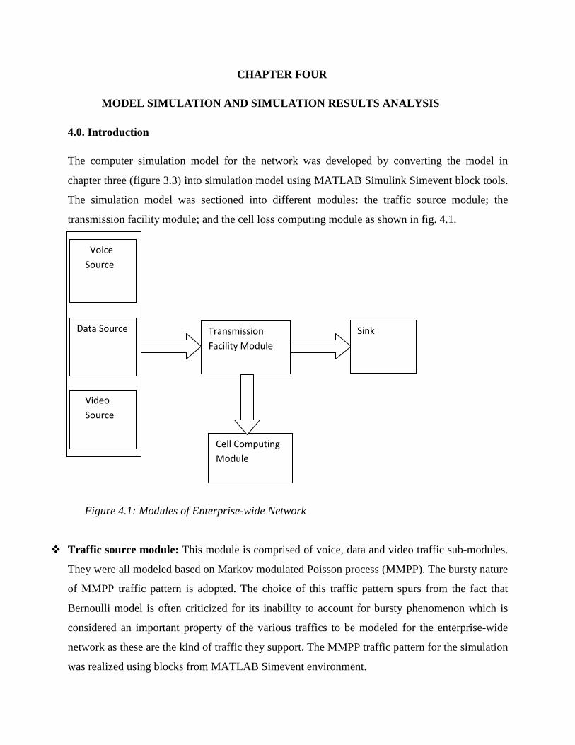
CHAPTER FOUR

MODEL SIMULATION AND SIMULATION RESULTS ANALYSIS

4.0. Introduction

The computer simulation model for the network was developed by converting the model in

chapter three (figure 3.3) into simulation model using MATLAB Simulink Simevent block tools.

The simulation model was sectioned into different modules: the traffic source module; the

transmission facility module; and the cell loss computing module as shown in fig. 4.1.

Figure 4.1: Modules of Enterprise-wide Network

� Traffic source module: This module is comprised of voice, data and video traffic sub-modules.

They were all modeled based on Markov modulated Poisson process (MMPP). The bursty nature

of MMPP traffic pattern is adopted. The choice of this traffic pattern spurs from the fact that

Bernoulli model is often criticized for its inability to account for bursty phenomenon which is

considered an important property of the various traffics to be modeled for the enterprise-wide

network as these are the kind of traffic they support. The MMPP traffic pattern for the simulation

was realized using blocks from MATLAB Simevent environment.

Cell Computing

Module

Voice

Source

Data Source

Video

Source

Transmission

Facility Module

Sink

Figure 4.2: Traffic source module

• Voice Source Sub-Module:This module was realized by modeling voice as MMPP

traffic to cater for the active and silent behavior of voice. This module as shown in fig. 4.3

comprise of Time Based Entity Generator which generates cells using an intergeneration time of

a statistical distribution (Poisson). The generated cell pass through an Enable Gate which is

regulated by a function call subsystem that is been controlled by an Entity Departure Event To

Function Call Block and whose basic function is to allow the carrier signal generated by a Time

Based Entity Generator that serves as an envelope for the cell generated thus providing a silent

and active form of traffic pattern for the voice traffic. The obtained pattern for the voice traffic

is shown in fig 4.4.

PABX

VOICE

Video Conf

VIDEO

IN1

IN2

IN3

OUT

Path Combiner

LAN

DATA

Figure 4.3: Voice Source Sub-Module

Figure 4.4: Traffic pattern from voice source

AverageIntergeneration

Time = 2

Average Time between On-Off

Points = 5

MARKOV-MODULATED POISSON ATM TRAFFIC SOURCE(PABX Trunk; Rate of Transmission = 2.048Mbps == Varying Packet Size *Recip(2,048E6) [transmission time]

1

Bursty-Source

OUT

Time-BasedEntity Generator

A2

IN

OUT

Set Attribute

round

RoundingFunction3

RandomSource

OUT

Generator 1

IN

Entity Sink

IN

OUT

f1

Entity Departure Event toFunction-Call Event

IN

en

OUT

Enabled Gate

Divide

f unction()

Out1

Create GeneratorSelection Variable

2.048E6

Constant

• Data Source Sub-Module: This module was realized by modeling data as MMPP traffic

to cater for the ON-OFF behavior of data traffic. This module as shown in fig. 4.5 comprise of

Time Based Entity Generator which generates cells (containing the data to be transmitted) using

an intergeneration time of a statistical distribution (Poisson with an exponential mean varying in

this case). The generated cell pass through an Enable Gate which is regulated by a function call

subsystem that is been controlled by an Entity Departure Event To Function Call Block and

whose basic function is to allow the carrier signal generated by a Time Based Entity Generator

that serves as an envelope for the cell generated thus providing a silent and active form of traffic

Pattern for the data traffic. The obtained pattern for the data traffic is shown in fig. 4.6.

Figure 4.5: Data Source Sub-Module


Time = 2


Points = 5

MARKOV-MODULATED POISSON ATM TRAFFIC SOURCE(Ethernet LAN; Rate of Transmission = 10Mbps == Varying Packet S ize *Recip(1E7) [transmission time]

1

Bursty-Source

OUT


A2

IN

OUT

Set Attribute

round

RoundingFunction2

RandomSource

OUT

Generator 1

IN

Entity Sink

IN

OUT

f1

Entity Departure Event toFunction-Call Event

IN

en

OUT

Enabled Gate

Divide

f unction()

Out1


1E7

Constant

Figure 4.6: Traffic pattern from data source

• Video Source Sub-Module: This module was realized by modeling data as MMPP

traffic to cater for the ON-OFF behavior of video traffic. This module as shown in fig. 4.7

comprise of Time Based Entity Generator which generates cells (containing the data to be

transmitted) using an intergeneration time of a statistical distribution (Poisson with an

exponential mean varying in this case). The generated cell pass through an Enable Gate which is

regulated by a function call subsystem that is been controlled by an Entity Departure Event To

Function Call Block and whose basic function is to allow the carrier signal generated by a Time

Based Entity Generator that serves as an envelope for the cells generated thus providing a silent

and active form of traffic pattern for the video traffic. The obtained pattern for the video traffic is

shown in fig 4.8.

Figure 4.7: Video Source Sub-Module

\ vf

fi

Figure 4.8: Traffic pattern from video source

MARKOV-MODULATED POISSON ATM TRAFFIC SOURCE(Video Conference JPEG - 1.554Mbps ==Varying Packet Size *Recip(1.554E6) [transmission time]


Points = 5


Time = 1

1

Bursty-Source

OUT


A2

IN

OUT

Set Attribute

round

RoundingFunction3

RandomSource

OUT

Generator 1

IN

Entity Sink

INOUT

f1

Enti ty Departure Event toFunction-Call Event

IN

en

OUT

Enabled Gate

Divide

f unction()Out1


1.554E6

Constant

� Transmission Facility Module: This module comprise of a first-in-first-out (FIFO)

transmission buffer queue with fixed capacity (ATM FIFO), an associated transmission link

single server(ATM SERVER) as shown in fig. 4.9. The single server was used because ATM

multiplexer was used for providing statistical multiplexing service for the BISDN service

supported by the network and carried via a leased ATM trunk.

Figure 4.9: Transmission facility module

� Cell computing module: The cell loss rate predicting module carries out computation

based on mathematical expression developed in chapter three. This expression where developed

based on fluid-flow approximation approach. The method assumes a uniform arrival and service

process – continuous information flowinstead of the discrete flow of cells. Fluid flow

approximation compares favorably with other existing and popularly accepted methods. This

module performs the computation of cell loss rate for the different traffic (homogeneous and

w

wait

RepeatingSequence

Stair

IN

tr

OUT

#d

Entity DepartureCounter

Display

IN

OUT

w

ATM FIFO

IN OUT

ATM SERVER

heterogeneous) supported by the network as shown in fig. 4.10. The module reads out minimum,

mean and maximum cell arrival rate during the course of simulation every one second and reads

in these values into the cell computing module where the cell loss is computed every second

during the course of running the simulation. The average of the cell loss is at the end of the

simulation obtained from this module.

Figure 4.10: Cell Computing Module

4.1 Simulation Model Validation

The model validation was carried out by comparing the result obtained from the proposed model

for investigating the behavior of enterprise-wide network that is based on leased trunk, and that

proposed in [54] for deriving network resources to support video related services in ATM. This

investigation was done in terms of cell loss rate and buffer capacity for different trunk capacity

of 30Mbps. The obtained result for the two models is shown in fig.4.11.

The set of curves obtained shows a similar behavior for the proposed model for computing cell

loss rate for video related traffic and that for traffic supported by enterprise-wide network. The

observed disparity is attributable to the fact that enterprise-wide network support both video

related traffic and other kind of traffic like voice and data.

AnalyticalResult1

prob

mu

lamda

pi1

tau

Out1

Probability for single source

Mean

mean1

From2max1

From1min1

From0.5

Constant3

Figure 4.11: Blocking probability against traffic intensity for video-related model and enterprise-wide

network traffic model for a trunk capacity of 30Mbps

4.2 Model Simulation

The key QoS parameters taken into consideration for the simulation include:

• Throughput: This is the intensity of traffic allowed into the network at a given time (i.e.

the amount of traffic the network can successfully handle at a given time)

• Buffer capacity: is the capacity of the buffer at the ATM access node

• Cell delay variation: is simply the variation in the time spent waiting in the queue.

• Cell loss rate: This is the ratio of number of cells rejected to the sum of the number of

cells in the queue and the number of cells rejected.

In order to carry out the performance evaluation on enterprise-wide network that is based on

leased trunk, with the aim of determining the effect of traffic overload on the network resource

(transmission capacity and buffer), the above QoS parameters were taken into consideration and

relationship established between them in the following order:

� Cell loss rate against traffic intensity for varying buffer size at varying trunk capacities.

� Cell delay variation against traffic intensity for varying buffer size at varying trunk

capacities.

cell

lo

ss r

ate

Traffic intensity(cells/second)

PB(video related sources)

PB(Enterprise source:D,V&VI)

� Cell loss rate and delay as a function of traffic intensity for varying buffer capacity.

� Cell loss rate and traffic intensity at a buffer capacity of 10(530Bytes).

� Cell loss as a function of buffer capacity for varying intensity.

� Cell loss rate and buffer capacity at a traffic intensity of 2.80E05cell/second.

The simulation was carried out with the range of values in mind for trunk capacity: 15M bps,

20Mbps, 30M bps and 40Mbps while for that of buffer capacity was varied in the range of: 5, 10,

15, 20 and 25. For the purpose of result generation, the simulation was run for 100seconds.

Readings were not taken for the first 5 seconds as the system gained stability at this point.

4.3 Simulation Results

The set of results obtained after running simulations of the model in order to carry out

performance evaluation on enterprise-wide network that is based on leased trunk, the effect of

traffic overload on the network resource (transmission capacity and buffer) are presented as thus:

4.3.1. Cell loss rate and Delay as a function Traffic Intensity for varying Buffer Capacity

for Homogeneous Traffic Source

In this case, the network was loaded with the individual type of traffic under consideration (i.e.

voice, data or video) and the behavior of the network was observed in order to understudy its

response in terms of the probability of the traffic been dropped and the delay variation

experienced by the traffic when the buffer capacity of the ATM access node is varied and when

the capacity of the leased trunk is varied. The set of results obtained are shown in Fig. 4.12 and

4.13, respectively. Figure 4.12 illustrates the obtained relationship between probability of cell

loss and average traffic intensity for varying buffer capacity at the ATM access node, while fig

4.13 shows the obtained relationship between cell delay and traffic intensity for varying trunk

capacity for the homogeneous traffic source.

Figure 4.12:Probability of cell loss against Traffic intensity for Varying Buffer Size(BC) at different trunk capacity

for homogenious traffic source (i.e. either Data or voice or Video).

Blo

ckin

g P

rob

ab

ilit

y

Traffic Intensity(cells/second)

Prob(BC=5)

Prob(BC=10)

Prob(BC=15)

Prob(BC=20)

Figure 4.13: Cell Delay against Traffic intensity for Varying for varying trunk capacity for Homogeneous

trafficsource (i.e. either Data or voice or Video).

The obtained curves as shown in fig. 4.12, shows a rising mean/average cell loss rate with

respect to traffic intensity for different buffer capacity. It is seen from the pattern of curves

obtained that as the traffic intensity increase, the probability of traffic drop in the network (cell

loss rate) also increases. Also it is seem from the set of curves obtained that as the capacity of the

buffer at the ATM access node increases, the probability of traffic being dropped decreases.

From the curve, it is seen that at traffic intensity between 5E5 and 1E6 that the probability of

traffic been dropped for the different buffer capacity of 5, 10, 15 and 20 is given as 0.86, 0.72,

0.62 and 0.53 respectively. These set of results shows an increased probability of traffic being

dropped as the capacity of the buffer becomes smaller. The observed behavior is attributable to

the fact that as the buffer capacity of the ATM access node is increased, the network is able to

accommodate more of the busty homogeneous traffic being transmitted in the network.

De

lay

(se

con

ds)


Delay( BW=15Mbps)

Delay (BW=20Mbps)

Delay(BW=30Mbps)

Delay(BW=40Mbps)

Similarly, fig. 4.13 shows a set of curve obtained from the investigation of cell delay against

traffic intensity for different trunk capacity ranging from 15Mbps, 20Mbps, 30Mbps, and

40Mbps respectively. From the curves obtained, it is seen that the average delay experienced by

the homogeneous traffic in the network lies within a constant value when the network is loaded

with traffic of different intensity from the homogeneous traffic source at varying trunk capacity.

From the family of curves obtained, it is seen that at a trunk capacity of 15Mbps, the average

delay experienced by traffic in the network is 1.4 E-11 while for a trunk capacity of 20Mbps, the

mean delay experienced by the traffic in the network is 7.6E-12.Also it is seen from the set of

curves obtained that at a trunk capacity of 30Mbps, the average delay experienced by the traffic

in the network is 2.49E-12 and finally, when the trunk capacity of the network was increased to

40Mbps, it is observed that the average delay experienced by traffic in the network is 1.08E-

12.These set of results shows that the delay experienced by traffic in the network decreases as

the capacity of the leased trunk acquired by the network is increased. This observed behavior is

attributable to the fact that as the bandwidth of the trunk increases, traffic experiences less delay

as there is little or no contention for available network resource during transmission.


for Heterogeneous Source (Data and Voice)

In this case, the network was loaded separately with the different combination of traffic under

consideration (i.e. voice and data) and the behavior of the network was observed in order to

understudy its response in terms of the probability of traffic been dropped and the delay variation

experienced by these traffic when the buffer capacity of the ATM access node is varied and

when the capacity of the leased trunk is varied. The set of results obtained as shown in fig 4.14

illustrate the relationship between probability of traffic drop in the network (cell loss rate) and

average traffic intensity at varying buffer capacity for the heterogeneous source. Similarly, fig.

4.15 shows the set of curves obtained when the network was observed for traffic delay at varying

traffic intensity at different trunk capacity under consideration.

Figure 4.14:Blocking Probaility against Traffic intensity for Varying Buffer Capacity(BC) for varying trunk

Bandwidth for Heterogenious Traffic Source(voice & Data)

The obtained curve as shown in fig. 4.14 shows a rising mean/average cell loss rate with respect

to traffic intensity for different buffer capacity. It is seen from the pattern of curves obtained that

as the traffic intensity increase, the cell loss rate also increases. Also it is seem from the set of

curves obtained that as the capacity of the buffer at the ATM access node increases, the

probability of traffic being dropped decreases. From the curve, it is seen that at a traffic intensity

of 3.0E05 that the probability of traffic being dropped for the different buffer capacity of 5, 10,

15 and 20 is given as 0.84, 0.73, 0.60 and 0.53 respectively. These set of results shows an

increased probability of traffic being dropped as the capacity of the buffer becomes smaller. The

observed fact is attributable to the fact that as the buffer capacity of the ATM access node is

increased, the network is able to accommodate more of the traffic being transmitted in the

network.

Blo

ckin

g P

rob

ab

ilit

y


Prob(BC=5)

Prob(BC=10)

Prob(BC=15)

Prob(BC=20)

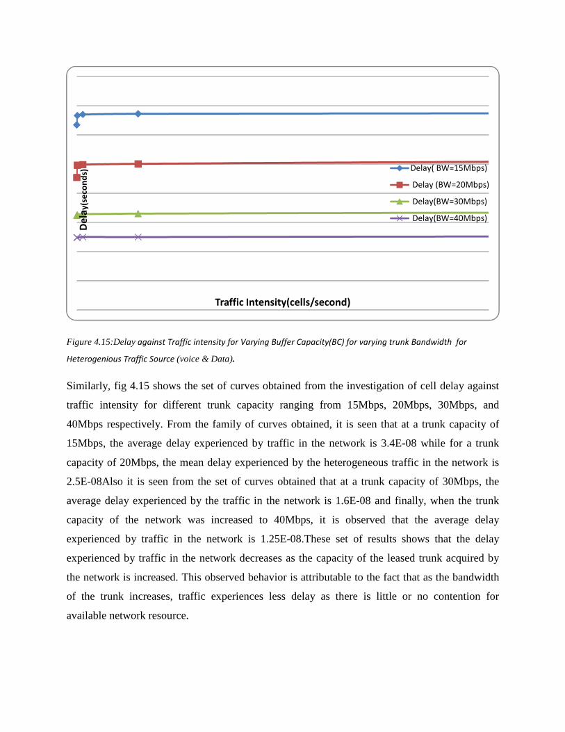
Figure 4.15:Delay against Traffic intensity for Varying Buffer Capacity(BC) for varying trunk Bandwidth for

Heterogenious Traffic Source (voice & Data).

Similarly, fig 4.15 shows the set of curves obtained from the investigation of cell delay against


40Mbps respectively. From the family of curves obtained, it is seen that at a trunk capacity of

15Mbps, the average delay experienced by traffic in the network is 3.4E-08 while for a trunk

capacity of 20Mbps, the mean delay experienced by the heterogeneous traffic in the network is

2.5E-08Also it is seen from the set of curves obtained that at a trunk capacity of 30Mbps, the

average delay experienced by the traffic in the network is 1.6E-08 and finally, when the trunk

capacity of the network was increased to 40Mbps, it is observed that the average delay

experienced by traffic in the network is 1.25E-08.These set of results shows that the delay

experienced by traffic in the network decreases as the capacity of the leased trunk acquired by

the network is increased. This observed behavior is attributable to the fact that as the bandwidth

of the trunk increases, traffic experiences less delay as there is little or no contention for

available network resource.

De

lay

(se

con

ds)


Delay( BW=15Mbps)

Delay (BW=20Mbps)

Delay(BW=30Mbps)

Delay(BW=40Mbps)


for Heterogeneous Source (Data, Voice and Video)

In this case, the network was loaded separately with the different combination of traffic under

consideration (i.e. voice, data and video) and the behavior of the network was observed in order

to ascertain the networks response in terms of the probability of traffic been dropped and the

delay variation experienced by these traffic when the buffer capacity of the ATM access node is

varied and when the capacity of the leased trunk is varied. The set of results obtained as shown

in fig 4.16 illustrate the relationship between probability of traffic drop in the network (cell loss

rate) and average traffic intensity at varying buffer capacity for the heterogeneous source.

Similarly, fig. 4.17 shows the set of curves obtained when the network was observed for traffic

delay at varying traffic intensity at different trunk capacity under consideration.

Figure 4.16:Blocking Probaility against Traffic intensity for Varying Buffer Capacity(BC) for varying trunk

Bandwidth for Heterogenious Traffic Source(Voice, Data& Video)

Blo

ckin

g P

rob

ab

ilit

y

Traffic Intensity

Prob(BC=5)

Prob(BC=10)

Prob(BC=15)

Prob(BC=20)

Figure 4.17:Delay against Traffic intensity for Varying Buffer Capacity(BC) for varying trunk Bandwidth for

Heterogenious Traffic Source (voice, Data& Video ).

The obtained curve as shown in fig. 4.16 shows a rising mean/average cell loss rate with respect

to traffic intensity for different buffer capacity. It is seen from the pattern of curves obtained that

as the traffic intensity increase, the cell loss rate also increases. Also it is seen from the set of

curves obtained that as the capacity of the buffer at the ATM access node increases, the

probability of traffic being dropped decreases. From the curve, it is seen that at a traffic intensity

between 2.0E6 and 2.5E6 that the probability of traffic being dropped for the different buffer

capacity of 5, 10, 15 and 20 is given as 0.84, 0.73, 0.61 and 0.53 respectively. This set of result

shows an increased probability of traffic being dropped as the capacity of the buffer becomes

smaller. The observed fact is attributable to the fact that as the buffer capacity of the ATM access

node is increased, the network is able to accommodate more of the busty traffic being transmitted

in the network.

De

lay

(se

con

ds)

Traffic Intensity(calls/second)

Delay( BW=15Mbps)

Delay (BW=20Mbps)

Delay(BW=30Mbps)

Delay(BW=40Mbps)

Similarly, fig. 4.17 shows a set of curve obtained from the investigation of cell delay against


40Mbps respectively. From the family of curves obtained, it is seen that at a trunk capacity of

15Mbps, the average delay experienced by traffic in the network is 6.7E-08 while for a trunk

capacity of 20Mbps; the mean delay experienced by the heterogeneous traffic in the network is

5.0E-08.Also it is seen from the set of curves obtained that at a trunk capacity of 30Mbps; the

average delay experienced by the traffic in the network is 3.2E-08 and finally, when the trunk

capacity of the network was increased to 40Mbps, it is observed that the average delay

experienced by traffic in the network is 2.5E-08. These set of results shows that the delay

experienced by traffic in the network decreases as the capacity of the leased trunk acquired by

the network is increased. This observed behavior is attributable to the fact that as the bandwidth

of the trunk increases, traffic experiences less delay as there is little or no contention for

available network resource.

4.3.4. Performance Analysis of the Network with respect to Cell Loss Rate and Traffic

Intensity at A Buffer Capacity of 10 (530Byte).

In this case, a comparison is done to ascertain the performance (utilization) of the network in

term of traffic drop when the network was loaded with the different traffic under consideration

and the capacity of the buffer at the ATM access node kept constant at 10(530Byte). Figure 4.18

shows the set of curve obtained. From the set of curves obtained, it is seem that there is a direct

relationship between cell loss rate and traffic intensity for the different traffic sources under

consideration as all curves follow almost the same pattern. Also from the set of curves as shown

in fig.4.16, it is also observed that at points where the traffic intensity lies between 3.0E05 and

7.0E05 that the homogeneous source experiences more traffic loss in the network as compared to

the other traffic types under consideration. This behavior is attributable to the fact that at this

points (i.e. between 3.0E05 and 7.0E05), the homogeneous source produces more busty traffic

which couldn’t be accommodated by the buffer at the access node therefore resulting in more

traffic drop as shown in the curves obtained.

Figure 4.18: Blocking Probability against Traffic Intensity at a Buffer Capacity of 10(530Byte) for homogeneous

and heterogeneous traffic sources.

4.3.5. Cell loss rate as a function of Buffer Capacity at varying Traffic Intensity for the

different Traffic Source.

In this case, a comparison is done to ascertain the behavior of the network in terms of cell loss

rate and buffer capacity when the network is loaded separately with the different combination of

traffic sources under consideration (i.e. homogeneous & heterogeneous sources) for a given

traffic intensity. The comparison was done by loading the network with the different traffic types

at given traffic intensity and observing its effect on the probability of traffic drop in the network

(cell loss rate or blocking probability) as the capacity of the buffer at the ATM access node is

varied in the range of 5, 10, 15 and 20. The set of curves obtained at this different traffic

Blo

ckin

g P

rob

ab

ilit

y


PB(Homo)

PB(Hetro:D&V)

PB(Hetro:D,V&VI)

intensities are shown in figures 4.19, 4.20 and 4.21 respectively for the different traffic sources

under consideration.

Figure 4.19: Blocking Probability against Buffer Capacity for homogeneous source at varying traffic intensity

The family of curves shown in fig. 4.19 represents the observed behavior of the network in terms

of cell loss rate and buffer capacity when the network was loaded with traffic from the

homogeneous source at varying intensity in the range of 5.00E04, 1.10E05, 2.20E05, 2.80E05

and 4.00E5cells/second respectively.

The set of curves obtained as shown in figure 4.19, shows that there is an inverse relationship

between cell loss rate and buffer capacity for a given traffic intensity i.e. as the buffer capacity

becomes smaller the network blocking probability of cells increases. This is attributable to the

fact that as the buffer capacity at the ATM access node reduces, it becomes unable to

accommodate more of the busty traffic generated by the homogeneous source at a given traffic

intensity, and as such drops some of this traffic in the network.

Blo

ckin

g P

rob

ab

ilit

y

Buffer Capacity

PB(TI=4E5)

PB(TI=2.8E5)

PB(TI=2.2E5)

PB(TI=1.1E5)

PB(TI=5E4)

The set of curves obtained, it can be easily decided what buffer capacity will support a particular

traffic intensity at a given QoS value (i.e. cell loss rate values). If we consider a buffer capacity

of 10, one can easily determine from the set of plots the individual QoS value for each traffic

intensity under consideration. It is seen from the plots that at a traffic intensity of 5.00E04, and at

an access node buffer capacity of 10, the QoS value the network will provide at this point is 0.20.

While at a traffic intensity of 1.10E05, and at an access node buffer capacity of 10, the QoS

value the network will provide will be 0.45. Similarly, at a traffic intensity of 2.20E05, and at an

access node buffer capacity of 10, the QoS value the network will provide will be 0.65.

Furthermore, at a traffic intensity of 2.80E05, and at an access node buffer capacity of 10, the

QoS value the network will provide will be 0.70. Finally, at a traffic intensity of 4.0E5, and at an

access node buffer capacity of 10, the QoS value the network will provide will be 0.78.

Figure 4.20: Blocking Probability against Buffer Capacity for heterogeneous source (Voice & Data) at varying

traffic intensity.

The family of curves as shown in fig. 4.20 represents the observed behavior of the network in

terms of cell loss rate and buffer capacity when the network was loaded with traffic from the

Blo

ckin

g P

rob

ab

ilit

y

Buffer Capacity

PB(TI=4E5)

PB(TI=2.8E5)

PB(TI=2.2E5)

PB(TI=1.1E5)

PB(TI=5E4)

heterogeneous source (i.e. data and voice) at varying intensity in the range of: 5.0E04, 1.1E05,

2.2E05, 2.8E05 and 4.0E5cells/second respectively.

The set of curves obtained as shown in fig. 4.20, it is seen that there is an inverse relationship

between cell loss rate and buffer capacity for a given traffic intensity i.e. as the buffer capacity

becomes smaller the probability of traffic drop in the network (blocking probability/cell loss

rate) increase. This observed behavior is attributable to the fact that as the buffer capacity at the

ATM access node becomes small, it becomes unable to accommodate more of the busty traffic

generated by the heterogeneous source (i.e. data and voice source) at specific traffic intensity,

and as such drops some of these traffic in the network.

From the set of curves obtained, one can be easily decided what buffer capacity will support a

particular traffic intensity at a given QoS value (i.e. cell loss rate) in the network. For example if

we consider a buffer capacity of 10, one can easily say from the set of plots the individual QoS

value for each traffic intensity under consideration. It is seen from the plots that at a traffic

intensity of 5.00E04, and at an access node buffer capacity of 10, the QoS value the network will

provide at this point is 0.26. While at a traffic intensity of 1.10E05, and at an access node buffer

capacity of 10, the QoS value the network will provide will be 0.44. Similarly, at a traffic


provide will be 0.65. Furthermore, at a traffic intensity of 2.80E05, and at an access node buffer

capacity of 10, the QoS value the network will provide will be 0.70. Finally, at a traffic intensity

of 4.00E5, and at an access node buffer capacity of 10, the QoS value the network will provide

will be 0.74.

Figure 4.21: Blocking Probability against Buffer Capacity for heterogeneous source (Voice, Data & Video) at

varying traffic intensity.

The family of curves as shown in fig. 4.21 represents the observed behavior of the network in

terms of cell loss rate and buffer capacity when the network was loaded with traffic from the

heterogeneous source (i.e. data, voice and video) at varying intensity in the range of: 5.0E04,

1.1E05, 2.2E05, 2.8E05 and 4.0E5cells/second respectively.

From the set of curves obtained as shown in fig. 4.21, it is seen that there is an inverse

relationship between cell loss rate and buffer capacity for a given traffic intensity i.e. as the

buffer capacity becomes smaller network blocking probability of cells increases. This observed

behavior is attributable to the fact that as the buffer capacity at the ATM access node reduces, it

becomes unable to accommodate more of the busty traffic generated by the heterogeneous source

(i.e. data, voice and video source) at specific traffic intensity, and as such drops some of these

traffic in the network.

Blo

ckin

g P

rob

ab

ilit

y

Buffer Capacity

PB(TI=4E5)

PB(TI=2.8E5)

PB(TI=2.2E5)

PB(TI=1.1E5)

PB(TI=5E4)

The set of curves obtained, one can be easily decided what buffer capacity will support a

particular traffic intensity at a given QoS value (i.e. cell loss rate) in the network. For example if

we consider a buffer capacity of 10, one can easily say from the set of plots the individual QoS

value for each traffic intensity under consideration. It is seen from the plots that at a traffic


provide at this point is 0.24. While at a traffic intensity of 1.10E05, and at an access node buffer

capacity of 10, the QoS value the network will provide will be 0.44. Similarly, at a traffic


provide will be 0.68. Furthermore, at a traffic intensity of 2.80E05, and at an access node buffer

capacity of 10, the QoS value the network will provide will be 0.70. Finally, at a traffic intensity

of 4.00E5, and at an access node buffer capacity of 10, the QoS value the network will provide

will be 0.76.

4.3.6 Performance Analysis of the Network with respect to Cell Loss Rate and Buffer

Capacity at a Traffic Intensity of 2.80E05.

The set of curves obtained as shown in fig. 4.22 shows an inverse relationship between cell loss

rate and buffer capacity for the traffic generated at an intensity of 2.80E05 by the different traffic

source under consideration. Form the set of curves obtained it is seen that the homogeneous

source experiences a constant cell loss rate of 0.60 for a buffer capacity between 15 and 20 while

the heterogeneous sources experience lesser cell loss at this points. This observed behavior is

attributable to the fact that the heterogeneous sources better utilizes the network resources as

they make more use of the buffer at the access node thereby reducing the traffic drop

experienced by the heterogeneous sources.

Figure 4.2: Blocking Probability against Buffer Capacity for homogeneous and heterogeneous traffic sources at a

traffic intensity of 2.80E05cells/second.

Blo

ckin

g P

rob

ab

ilit

y

Buffer Capacity

PB(Homo)

PB(Hetr:D&V)

PB(Hetr:V,D&V)

CHAPTER FIVE

CONCLUSION AND RECOMMENDATION

5.0 Conclusion

This thesis introduces communication system, with a quick review of the explosive growth that

telecommunication has witnessed over the years in the area of services they support and

technology. This is basically attributable to the break though in digital electronics and very large

scale integrated circuit (VLSIC). It further classified communication networks based on: there

geographical spread of the nodes and host. In this case, networks such as LAN, MAN, WAN

were reviewed and their state of art technology, operating protocol and frame formats. Also

communication networks were classified based on the model employed by the nodes. In this

case, broadcast and switched networks were reviewed. Furthermore, networks were classified

based on their access restriction and in this case networks were grouped into private and public

networks and a review of theirsupporting technologies, protocol of operation and frame/cell

format was also carried out.

This thesis was further narrowed down to Enterprise-wide network which is a private network. A

review of the services supported by this network, and the supporting state of the art technology

was also carried out. From the review it was found out that currently enterprise-wide network

support broadband service and ATM has been chosen as the supporting technology BISDN. This

further narrowed the review to ATM technology, its protocol of operation and cell format.

Due to the fact that enterprise-wide networks are geographically separated from each other, there

is need for continuous communication from the different sites of the network owned by corporate

entities. Therefore the need to connect them together via leased trunks (backbone) from public

network as most enterprise cannot afford the cost of running and maintain a direct backbone

trunk to all their sites geographically separated.

In order to carry out the specific objectives of this research, network architecture of fixed LAN,

WLAN and PABX was adopted and a physical model was developed having bearing in mind the

supporting services and technology. After this, a model developed in order to carry out an

analysis of the specific objective of this thesis. The adopted model was further simulated using

MATLAB Simulink environment and the results of the QoS parameters under investigation were

obtain from the cell loss predicting module in the computer simulation model. The obtained

results were analyzed using Microsoft Excel.

5.1 Observation

From the analysis of the set of results obtained, it was seen that there is a relationship between

the transmission capacity (i.e. trunk capacity/bandwidth) and the delay experienced by traffic in

the network. From the result obtained and analyzed in the previous chapter, it was also observed

that the delay experienced by traffic is usually constant for a particular trunk capacity.

Furthermore, it was also observed that the delay experienced by traffic in the network decreases

as the capacity of the trunk increase.

Similarly, it was also observed from the set of results obtained that there is a direct relationship

with traffic intensity and the blocking probability (i.e. the probability of traffic being dropped in

the network). From the set of result obtained, it was observed that there is also an inverse

relationship between cell loss rate and buffer capacity of the buffer at the ATM access node at

given traffic intensity for the different traffic considered in the network. From the observed

behaviors, it was seen that as the capacity of the buffer at the access node was increased, the

probability of traffic drop in the network decreases for the different traffic type under

consideration in the network.

From this observed behaviors, and the set of curves obtained one designing a network to support

any of the traffic type under consideration in this thesis can determine the optimum resources

that will be required to support a particular QoS value.

Finally the set of result obtained on comparing the different sources with respect to average

utilization of the network resources shows that the heterogeneous source (i.e. data, voice and

video) better utilizes the network resource more than the heterogeneous source (i.e. data and

voice) at any given traffic intensity while homogeneous traffic source, least utilizes the network

resources.

5.2. Recommendation

We have seen from the results obtained in this thesis that, one can easily determine the optimum

network resource that would be needed to support traffic at a given QoS (i.e. cell loss rate) value

for a network that support the different traffic under consideration in this thesis.

We therefore recommend that QoS (i.e. jitter) be also considered for investigation for the same

set of traffic types considered in this thesis.

Finally, we also recommend that other traffic types be considered for the same analysis in terms

of cell loss rate and jitter.

REFERENCES

[1] Michael Duck and Richard Read, “Data Communications and Computer Networks for

Computer Scientists and Engineers,” Pearson, Prentice Hall 2nd Edition 2003.

[2] http://en.wikipedia.org/wiki/Enterprise_private_network.

[3] AchillePattavina, “Switching Theory Architectures and Performance in Broadband ATM

Networks”, John Wiley & Sons Ltd (1998).

[4] Dr. Sanjay Sharma, “Communication Systems (Analogue and Digital)”, S.K. Kataria& Sons,

New Delhi 6th Edition 2013.

[5] J. Dunlop and D.G Smith, “Telecommunication Engineering”, Thomson Press (India), New

Delhi Chapman &Hall 3rd Edition 1994

[6] Roger L. Freeman, “Telecommunication System Engineering”, John Wiley & Sons, Inc.,

Hoboken, New Jersey, 4th Edition 2004.

[7] R. Handel, M. N. Huber, and S. Schroder, ATM Networks: Concepts, Protocols,

Applications, Addison-Wesley, 1994.

[8] P.Gnanasivam, “Telecommunication Switching and Networks”, New Age International

Publisher, New Delhi India 2nd Edition 2004.

[8] P.Gnanasivam, “Telecommunication Switching and Networks”, New Age International

Publisher, New Delhi India 2nd Edition 2004.

[9] Leon, Gracia and Widjaja, “Communication Networks, Fundamental Concepts and Key

Architectures” Thomson Press (India), New Delhi Chapman &Hall 3rd Edition 1994

[10] David D. C, Kenneth T. P, and David P. W, “An Introduction to Local Area Networks”,

IEEE, Vol. 66, no. 11, November 1978.

[11] DrZhili S, “Components of Data and Internet Networking, LANs, High Speed LANs and

LAN Interconnections” University of Surrey Guildford Surrey, 2010.

[11] DrZhili S, “Components of Data and Internet Networking, LANs, High Speed LANs and

LAN Interconnections” University of Surrey Guildford Surrey, 2010.

[12]Mitchell B, “Computer and Wireless Networking Basics”. March 1, 2010,

http://compnetworking.about.com/od/basicneworkingconcepts/u/computer_networking_basi

cs.htm

[13] M. Conti, E. Gregori and L. Luciano, “Metropolitan Area Networks”, London: Springer-

Verlag, 1997.

[14] A. S. Tanenbaum, Computer Networks, 4th Edition, New Jersey: Prentice Hall, 2003.

[15] M. N. O. Sadiku, “Metropolitan Area Networks”, Boca Raton: CWC Press, 1994.

[16] R. Horak, “Telecommunications and Data Communications Handbook”, New Jersey: John

Wiley & Sons, Inc., 2007.

[17] M. N. Sadiku and M. M. Sarhan, “Performance Analysis of Computer Networks”, Cham:

Springer, 2013.

[18] BICSI, “Network Design Reference Manual”, 2009.

[19] M. P. Clark, “Networks and Telecommunications: Designs and Operation”, Second Edition,

West Sussex: JOHN WILEY & SONS, 1997.

[20] C. J. Wells, "Telecommunications-Computer Networks - Wide Area Networks," [Online].

Available:

http://www.technologyuk.net/telecommunications/networks/wide_area_networks.shtml.

[Accessed 28 April 2015].

[21] W. Richard Stevens, “TCP/IP Illustrated, Volume1, The Protocols”, Addison Wesley 2015

[22]Robert J. Roden and Deborah Taylor, "Frame Relay Networks", Digital Technical Journal,

vol. 5 No 1, Winter 1993.

[23]Uyless Black, “Frame Relay Networks : specifications and implementations”, McGraw-Hill,

1994,

[24] William Stallings, “ISDN and Broadband ISDN with Frame Relay and ATM”, Prentice-

Hall, 3rd Edition 1995.

[25] Nathan J. Muller and Robert Davidson, “The Guide to Frame Relay and Packet

Networking”, Prentice-Hall 1994.

[26] McDysan, David and Spohn, Darren, “ATM Theory and Applications, Signature

Edition”: McGraw Hill (1999)

[27] Buchanan, W., “Advanced Data Communications and Networks”: Chapman & Hall

(1997)

[28] ITU-T Recommendation Q.2931, “Broadband Integrated Services Digital Network

(B-ISDN) – Digital Subscriber Signalling No. 2 (DSS 2) – User-Network Interface (UNI)

Layer 3 Specification for Basic Call/Connection Control” (Feb 1995)

[29] ATM Forum Technical Committee, ATM Forum AF-CS-0135.000, “PHY/MAC

[30] ATM Forum Technical Committee, ATM Forum AF-SAA-0049.001, “Audiovisual

Media Services: Video On Demand Specification 1.1” (Mar 1997)

[31] ATM Forum, “ATM User-Network Interface Specification Version 3.1”, PTR Prentice Hall,

1995.

[32] G. Guerin, H. Ahmadi and M. Naghshineh, “Equivalent Capacity and its Application to

Bandwidth Allocation in High-speed Networks,” IEEE J. Select. Areas in Communications,

Vo1.9, No.7, pp.968-981, Sept. 1991

[33] Keshav, S, “An Engineering approach to Computer Networking : ATM networks, the

Internet, and the Telephone network” Addison-Wesley 1997.

[34]Luhar D. R, “Introduction to Public Switched Telephone Networks (PSTNs): POTS, ISDN,

DLC, DSL, and PON Technologies, Systems and Services”, Sigma Publishing India, 2006.

[41] Aranuwa, F.O,” Traffic Control and Bandwidth Allocation in ATM Networks”, Conference

Paper at AdekunleAjasin University, Akungba – Akoko, 2010.

[42] C. Beard and V. Frost, “Dynamic agent-based prioritized connection admission for stressed

networks,” in 1999 IEEE Int. Conf. Communications, Vancouver, B.C., Canada, June 1999.

[43] International Telecommunication Union, Telecommunication Standardization Sector,

“International Emergency Preparedness Scheme,” ITU Recommendation, E.106, Mar. 2000.

[44] Computer Science and Telecommunications Board (CSTB), National Research Council,

Computing and Communications in the Extreme: “Research for Crisis Management and Other

Applications”, Washington, DC: National Academy Press, 1996.

[45] C. Beard, “Dynamic agent based prioritized resource allocation for stressed networks,”

Ph.D. dissertation, Univ. of Kansas, Lawrence, 1999.

[46] R. Rajanet al., “A policy framework for integrated and differentiated services in the

Internet,” IEEE Network Mag., pp. 36–41, Sept./Oct.1999.

[47] S. Jordan and P. Varaiya, “Control of multiple service, multiple resource communication

networks,” IEEE Trans. Commun., vol. 42, pp. 2979–2988, Nov. 1994.

[48] K. W. Ross, “Multiservice Loss Models for Broadband Telecommunication Networks”,

London, U.K.: Springer-Verlag, 1995.

[49] B. Kraimeche and M. Schwartz, “Circuit access control strategies in integrated digital

networks,” in IEEE INFOCOM, San Francisco, CA, Apr.1984, pp. 230–235.

[50] P. B. Key, “Optimal control and trunk reservation in loss networks,” Probabil. Eng. Inform.

Sci., vol. 4, pp. 203–242, 1990.

[51] Ness B. Shroff, and MischaSchwartz , “Improved Loss Calculations at an ATM

Multiplexer” IEEE/ACM transactions on Networking, vol. 6, no. 4, August 1998

[52] Vigil Dobrotal and Daniel Zinca, “Traffic model for data, voice and video source in ATM”

IEEE Proc-Commun., Vol 142, No. 4 August 1997.

[53] Bijan J. and Ferit Y., “An Efficient Method For Computing Cell Loss Probability for

Heterogeneous Bursty Traffic in ATM Network”, Electrical and Computer Engineering

Department, George Manson University,John Wiley & Son Ltd.,1992.

[54] C.I. Ani, Fred H. and Riaz A, “Methodology for Derivation of Network Resources to

Support Video Related Service in ATM Based Private WAN” IEEE Proc-Commun., Vol 142,

No. 4 August 1994..

[55] Ivy and Jean, “Dynamic Bandwidth Allocation in ATM switches”, Journal of Applied

probability,1995.

[56] Ani C.I., “Determination of optimum number of trunk line for corporate network backbone

in Nigeria”, Nigerian Journal of Technology, Vol. 23, No. 1, March 2004.

[57] Song C, San-qi Li and Joydeep G, “dynamic bandwidth allocation for effective transport of

real time vbr video over ATM”, University of Texas at Austin IEEE 1994

[58] Sykas D, et. al., "Congestion Control – Effective Bandwidth Allocation in ATM Networks",

High Performance Networking.IV (C-14), IFIP, Belgium, 1993, pp.65-80.

[59] Roch Guerin, Hamid Ahmadi and Mahmoud Naghshineh, "Equivalent Capacity and its

Application to Bandwidth Allocation in High Speed Networks" IEEE Journal on Selected Areas

in Communications.Vol. 9 .No. 7, September 1991 pp.968-981.

[60] C. l. Ani& Fred Halsali, "Simulation Technique for evaluating Cell-Loss Rate In ATM

Networks"; The Society for Computer simulation. SIMULATION Journal California; Vol. 64,

No.5: May 1995; pp. 320-329.

AJIBO CHINENYE AUGUSTINE

Documents

Transcript of AJIBO CHINENYE AUGUSTINE