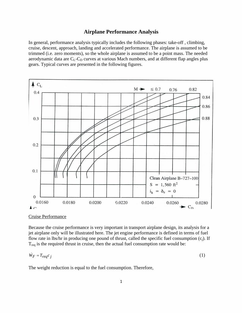
1

Airplane Performance Analysis

In general, performance analysis typically includes the following phases: take-off , climbing, cruise, descent, approach, landing and accelerated performance. The airplane is assumed to be trimmed (i.e. zero moments), so the whole airplane is assumed to be a point mass. The needed aerodynamic data are CL-CD curves at various Mach numbers, and at different flap angles plus gears. Typical curves are presented in the following figures.

Cruise Performance Because the cruise performance is very important in transport airplane design, its analysis for a jet airplane only will be illustrated here. The jet engine performance is defined in terms of fuel flow rate in lbs/hr in producing one pound of thrust, called the specific fuel consumption (cj). If Treq is the required thrust in cruise, then the actual fuel consumption rate would be:

jreqF cTW = (1) The weight reduction is equal to the fuel consumption. Therefore,

2

dtcTdtWdW jreqF −=−= (2) The specific endurance, or endurance factor, is defined as the time in hrs flown per pound of fuel and is given by:

lbshrscTdw

dtjreq

/,1−= (3)

The specific range, or range factor, is defined as the distance travelled per pound of fuel and is given by: (using the relation: V=ds/dt)

lbsnmcT

VdWds

jreq/,−= (4)

Since

WCCW

LDDT

LD

req ===

it follows that

jDL

WcCCV

dWds )/(

−= (5)

But the flight speed can be written as:

LSCWV

ρ2

= (6)

Therefore,

WdW

CC

ScdWds

DL

j

−=

ρ2

689.11 , in nm/lbs (7)

Eq. (7) shows that for a given weight and altitude, the range is maximum if DL CC / is maximized. Assuming constant air density, cj and DL CC / , Eq. (7) can be integrated exactly to give:

( )endbeginDL

jWW

CC

ScR −=

ρ675.1 , in nm (8)

For the endurance, Eq. (3) is written as

jDL

WcCC

dWdt /

−=

Therefore, the endurance is given by:

3

=

end

begin

DL

j WW

nCC

cE

1 , in hrs. (9)

Eqs. (8) and (9) are called Breguet equations for range and endurance of jet airplanes.

On the other hand, a jet airplane may cruise at a constant true speed or Mach number. In this case, Eq. (5) is directly integrated to give, with constant cj and CL/CD,

end

begin

jDL

WW

nc

CVCR /

= (10)

Since V=MVa, where Va is the speed of sound, Eq. (10) can also be written as:

end

begin

jDLa

WW

nc

CMCVR

=

/ (11)

Eq. (10) is frequently used to determine the combat radius of a fighter at a specified speed. Eq. (11) is further used to determine the best cruise Mach number as shown in the figure below.

The constant speed endurance is still given by Eq. (9).

As shown in Eq. (8), to maximize the range, the ratio, DL CC / must be maximized. In cruise, a parabolic drag equation is a valid assumption. Therefore, the following ratio is to be maximized:

20 LD

LkCC

Cf

+=

4

where k = 1/πAe. By setting df/dCL to 0, it can be shown that

20 3 LD kCC = (12)

On the other hand, if CL/CD is to be maximized, then

20 LD kCC = (13)

Eq. (12) is used to determine CL for the maximum range and hence the speed through Eq. (6). Based on Eq. (12), CL obtained tends to be small, and hence the flight speed is high. If the corresponding Mach number exceeds the drag divergent Mach number, the flight speed must be reduced to one corresponding to a Mach number slightly below Mdiv.

5

6

Stall Speeds and Minimum Speeds

The 1-g stall speed is defined by

trimLs SC

WVmax,

2ρ

= (14)

However, if the airplane is not controllable at αstall, CLmax in Eq. (14) must be replaced with CLmax, controllable. Because Vs affects greatly the performance of the airplane in take-off, landing, approach and climb, it is required to determine it through flight test with the requirements that the speed reduction to the minimum speed does not exceed one knot per second; the C.G. at the most critical location (usually means the most forward); and at zero thrust. Of course, it is also evaluated at various flap angles.

Level Flight Maximum Speeds and Ceilings

Maximum thrust is a function of altitude and Mach number: Tmax(δ,M), where δ=p/p0. With a parabolic drag equation, Tmax(δ,M) can be written as:

AeSqW

WSqMC

WMT D

πδ

δδδ /

/)(

/),( 0max += 23.1481 Mq δ= (15)

Eq. (15) can be used to graphically determine the maximum level flight Mach numbers and absolute ceilings at a given weight and altitude.

Flight Envelope

A typical V-n diagram is presented in the following.

7

Note that the stall speed in the V-n diagram may be computed from

SCWV

ND

smax

2ρ

= , 22maxmax )( DLN CCC += , CD at CLmax (16)

VA is the design maneuvering speed and is estimated as

limnVV sA =

where nlim = Llim/W (the load factor) and is specified as 2.5 for a jet transport.

VC is the design cruising speed and is defined by the designer.

VD is the design diving speed and must satisfy:

VD ≥ 1.25VC

Maneuvering in a vertical plane

In an instantaneous pull-up maneuver, the lift is equal to nW. Therefore, from an aerodynamic point of view,

8

LL

sLs

LC

C

VV

SCV

SCVW

Ln max2

2

max2

max2

maxmax

5.0

5.0====

ρ

ρ (17)

It is seen from Eq. (17) that when n is plotted versus speed, the curve is parabolic (i.e. varies with V2). However, in a sustained pull-up maneuver, there must be enough thrust to overcome the drag. In this case, “n” is solved from;

SqAe

nCCDT LD ))((

20 π+== (18)

At a high speed, a jet airplane is mostly limited by the available thrust in maneuvering.

Maneuvering in a horizontal plane

In a steady level and coordinated turn, the following equations are satisfied:

WL =φcos (19)

9

..sin2

FCR

Vg

WLt==φ (20)

Note that “coordinated turn” means there is no side force. From Eq. (19), the load factor in a level and coordinated turn is therefore

φcos1

==WLn (21)

The radius of turn is obtained from Eq. (20):

1tan 2

22

−==

ng

Vg

VRt φ (22)

The turn rate is given by

tRV

=ψ (23)

Note that in any maneuver, the stall speed becomes a function of the load factor. Eq. (17) is still valid:

nVV gsturns )1()( −= (24)

Example 3 An airplane is flying straight and level at sea-level and at a speed of 300 ft/sec. The pilot puts the airplane in a level, coordinated turn with a radius of 2,850 ft, while maintaining the same angle of attack as the one the airplane had in the straight and level flight condition. The pilot adjusts the engine thrust as required to maintain the speed at 300 ft/sec (i.e. sustained turn). Determine the required thrust.

10