Airplane Dynamics, Modeling, and Controlpmarzocc/AE430/Reports/Lecture.pdf · Airplane Dynamics,...
27
Airplane Dynamics, Modeling, and Control Dr. Eugene A. Morelli NASA Langley Research Center May 14, 1997
Transcript of Airplane Dynamics, Modeling, and Controlpmarzocc/AE430/Reports/Lecture.pdf · Airplane Dynamics,...

Airplane Dynamics, Modeling, and Control
Dr. Eugene A. Morelli
NASA Langley Research Center
May 14, 1997

Overview
● General Airplane Dynamics
● Modeling for Control Design
● Control Design for Airplanes
● Demonstrations

Airplane Dynamics
● The Airplane is a Nonlinear Dynamical System
● Newton’s 2nd Law for a Rigid Body
r ˙ p =
r F ∑• Translational Motion :
r ˙ h =
r M ∑• Rotational Motion :

Assumptions
● Earth is an inertial reference, no curvature
● Airplane is a rigid body with lateral symmetry
● Thrust acts along fuselage through the c.g.
● Still atmosphere (no winds, no gusts)
● Constant mass, no internal mass movements

Axis Systems
● Equations written in body axes
– Fixed to the airplane, constant inertia
– Rotating axes nonlinear inertial terms
xeye ze
xb
zbyb
Earth

Nonlinear Equations of Motion
Translational motion of the c.g.
Rotational motion about the c.g.
mr ˙ V +
r ω × m
r V =
r F aero +
r F prop +
r F gravity
Ir ˙ ω +
r ω × I
r ω =
r M aero
Rotational kinematics
r ˙ Θ = L
r ω

States and Controls
q
r
p
v
w
u
V
−δe
−δa
−δ r
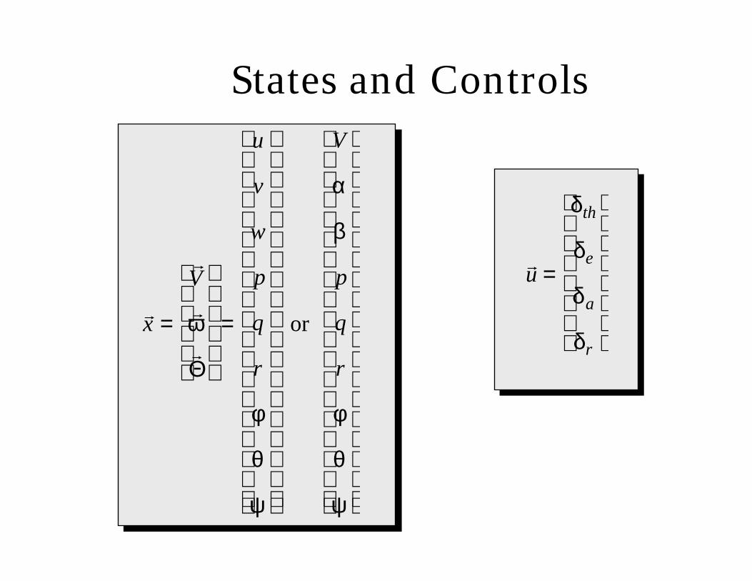
States and Controls
r x =
r V r ω r Θ
=
u
v
w
p
q
r
φ
θ
ψ
or
V
α
β
p
q
r
φ
θ
ψ
r u =
δth
δe
δa
δr

Steady Flight
● Nonlinear Equations of Motion :
● Define steady state (trim) :
r ˙ x =
r f
r x ,
r u ( )
r 0 =
r f
r x o ,
r u o( )
L
D
L t
W
M o
αV
α
Μ
unstable
stable
TRIM
T
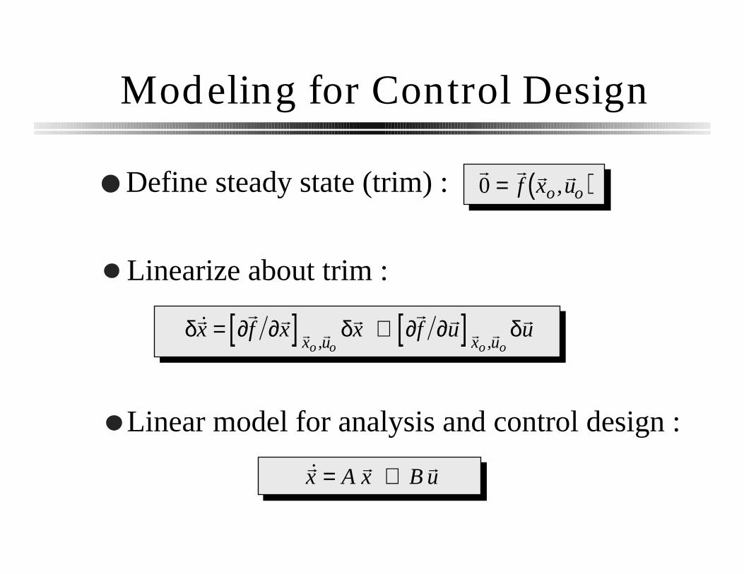
Modeling for Control Design
● Define steady state (trim) :
Linear model for analysis and control design :
Linearize about trim :
r 0 =
r f
r x o ,
r u o( )
δr ˙ x = ∂
r f ∂r
x [ ] r x o ,
r u o
δr x + ∂
r f ∂ r
u [ ] r x o ,
r u o
δ r u
r ˙ x = A
r x + B
r u
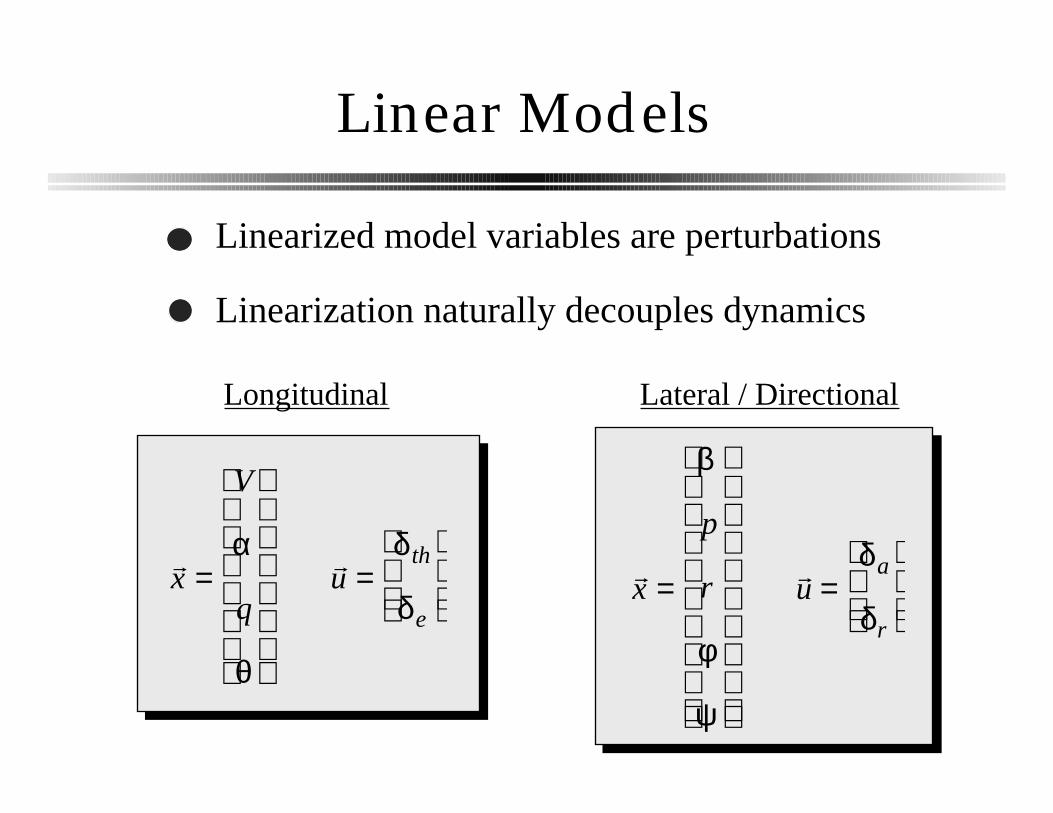
Linear Models
Longitudinal Lateral / Directional
Linearized model variables are perturbations
r x =
V
α
q
θ
r u =
δ th
δe
r x =
β
p
r
φ
ψ
r u =
δa
δr
Linearization naturally decouples dynamics

Longitudinal Linear Equations
˙ α = ZV V + Zα α + q + Zδeδe
˙ V = XV + TV( )V + Xα α − gθ + Tδthδ th + Xδe
δe
˙ q = MV V + Mα α + Mq q + Mδeδe
˙ θ = q

Laplace Transform
s ˜ α = ZV˜ V + Zα ˜ α + ˜ q + Zδe
˜ δ e
s ˜ V = XV + TV( ) ˜ V + Xα ˜ α − g ˜ θ + Tδth˜ δ th + Xδe
˜ δ e
s ˜ q = MV˜ V + Mα ˜ α + Mq ˜ q + Mδe
˜ δ e
s ˜ θ = ˜ q

Computing Transfer Functions
s − XV + TV( ) −Xα 0 g
−ZV s − Zα −1 0
−MV −Mα s − Mq 0
0 0 −1 s
˜ V
˜ α
˜ q
˜ θ
=
TδthXδ e
0 Zδ e
0 Mδe
0 0
˜ δ th˜ δ e

Computing Transfer Functions
˜ α ˜ δ e
=
s − XV + TV( ) Xδ e0 g
−ZV Zδ e−1 0
−MV Mδes − Mq 0
0 0 −1 ss − XV + TV( ) −Xα 0 g
−ZV s − Zα −1 0
−MV −Mα s − Mq 0
0 0 −1 s

Modeling Example
Airplane : F-16
Flight Condition : 5º AOA 10,000 ft 350 kts
c.g. position : 0.2 (fwd)c
Full Linear Model
Short Period Approx.
˜ α ˜ δ e
=−0.19 s + 0.008[ ]2 + 0.08 2( )
s + 0.008[ ]2 + 0.07 2( ) s +1.3[ ] 2 + 2.9 2( )
˜ α ˜ δ e
= −0.19
s +1.3[ ]2 + 2.9 2( )

Why Feedback Control?
● Modify plant dynamics
● Accurate regulation or tracking
● Overcome plant uncertainty
+
–
r e u y
b
n
Controller Plant
K SAS
–
+
Sensors

Airplane Control Tasks
● Stability Augmentation System (SAS)
● Control Augmentation System (CAS)
» pitch rate command system
» g-load command system
● Autopilots (pilot relief)» airspeed hold
» altitude hold
» heading hold
» turn coordination

Choosing Feedback Quantity
Stability Augmentation
˙ q = Mα α + Mq q + MδeδeSAS
+ δePILOT( )
δeSAS= K α
˙ q = Mα + K Mδe( )effective Mα
1 2 4 4 3 4 4 α + Mq q + Mδ e
δePILOT

Stability Augmentation System (SAS)
K
–
+
δeSAS
αδe
δePILOT α

SAS Design Demonstration
Airplane : F-16
Flight Condition : 5º AOA 10,000 ft 350 kts
c.g. position : 0.2 (fwd)c
Short Period Approx.
˜ α ˜ δ e
= −0.19
s +1.3[ ]2 + 2.9 2( )
Full Linear Model
˜ α ˜ δ e
=−0.18 s + 0.007[ ] 2 + 0.08 2( )
s + 0.08[ ]2 + 0.13 2( ) s +1.8( ) s − 0.1( )
c.g. position : 0.35 (nom)c

Choosing Feedback Quantity
Regulation or Tracking
+
–
e VController
Sensor
δth Vδth
r = VDESIRED
Airplane
= 0 to hold trim airspeed

Airspeed Hold Demonstration
Airplane : F-16
Flight Condition : 5º AOA 10,000 ft 350 kts
c.g. position : 0.2 (fwd)c
Full Linear Model
˜ V ˜ δ th
=0.17 s +1.3[ ] 2 + 6.12( ) s + 0.8( )
s + 0.008[ ]2 + 0.07 2( ) s +1.3[ ] 2 + 2.9 2( )

Control System Design
● Close feedback control loops
» one at a time (classical control)
» many at once (modern control)
● Use several linear models design points
● Link individual designs (gain scheduling)

Practical Considerations
● Control Effectiveness» Deflection limits
» High AOA» Nonlinearity
» Actuator Dynamics
● Time delay» Control surface rate limits
» Transport delay
● Unmodeled effects● Pilot variability

Control Design
Nonlinear AirplaneDynamic Model
LinearDesignModels
ControlDesign
NonlinearBatch
Simulation
PilotedNonlinearSimulation
Flight Test

Summary
● General Airplane Dynamics
● Modeling for Control Design
● Control Design for Airplanes
● Demonstrations
● References for Further Study