AIRCRAFT FLIGHT DYNAMICS AND CONTROL - Ira A....
219
AIRCRAFT FLIGHT DYNAMICS AND CONTROL August 30, 2008 Dennis S. Bernstein Department of Aerospace Engineering The University of Michigan Ann Arbor, MI 48109-2140 [email protected] Copyright 2008
Transcript of AIRCRAFT FLIGHT DYNAMICS AND CONTROL - Ira A....

AIRCRAFT FLIGHT DYNAMICSAND CONTROL
August 30, 2008
Dennis S. BernsteinDepartment of Aerospace EngineeringThe University of MichiganAnn Arbor, MI [email protected]
C o p y r i g h t 2 0 0 8


Contents
Chapter 1. Review of Kinematics 3
1.1 Points, Particles, and Bodies 3
1.2 Physical and Mathematical Vectors 3
1.3 Dot Product 5
1.4 Angle Vector and Cross Product 6
1.5 Frames 8
1.6 Signed Angles 11
1.7 Particle-Fixed Frames 11
1.8 Physical Matrices 12
1.9 Physical Cross Product 15
1.10 Rotation and Orientation Matrices 18
1.11 Euler’s Theorem 24
1.12 Quaternions 29
1.13 Euler Angles 29
1.14 Frame Derivatives 33
1.15 Momentum 34
1.16 Angular Momentum 35
1.17 Angular Velocity Vector 35
1.18 Euler Angle Derivatives 40
1.19 Transport Theorem 41
1.20 Double Transport Theorem 43
1.21 Summation of Angular Velocities 44
1.22 Solid and Open Frame Dots 45
1.23 Problems 45
Chapter 2. Aircraft Kinematics 49
2.1 Frames Used in Aircraft Dynamics 49
2.2 Velocity Vector 52
2.3 Rotational Kinematics 57
2.4 Vector Derivatives in Rotating Frames 59
2.5 Cross Product 60
2.6 Problems 61
Chapter 3. Review of Dynamics 65

iv CONTENTS
3.1 Newton’s First Law for Particles 65
3.2 Newton’s Second Law for Particles 66
3.3 Forces and Moments 66
3.4 Change in Angular Momentum 68
3.5 Momentum and Angular Momentum Relative to Centerof Mass 74
3.6 Continuum Bodies 77
3.7 Properties of the Inertia Matrix 78
3.8 Problems 79
Chapter 4. Aircraft Dynamics 81
4.1 Flight Dynamics and Control 81
4.2 History of Aircraft Stability and Control 81
4.3 Aerodynamic Forces 81
4.4 Translational Momentum Equations 83
4.5 Rotational Momentum Equations 87
4.6 Aircraft Equations of Motion Resolved in FAC 89
4.7 Problems 90
Chapter 5. Linearization 93
5.1 Taylor series 93
5.2 Alternative Linearization Procedure 94
5.3 Trigonometric Functions 94
5.4 Steady Flight 95
5.5 Linearization of the Aircraft Kinematics 96
5.6 Linearization of the Aircraft Dynamics in FAC 97
5.7 Linearization of the Aircraft Dynamics in FSf98
5.8 Problems 101
Chapter 6. Static Stability and Stability Derivatives 105
6.1 Control Surface Deflections 105
6.2 Aerodynamic Force Coefficients 105
6.3 Linearization of Forces in FSf108
6.4 Aerodynamic Moment Coefficients 115
6.5 Linearization of Moments in FSf124
6.6 Effect of Adverse Control Derivatives 126
6.7 Problems 127
Chapter 7. Linearized Equations of Motion 129
7.1 Longitudinal Equations of Motion 129
7.2 Linearized Longitudinal Equations and Transfer Functions 131
7.3 Lateral Equations of Motion 133
7.4 Linearized Lateral Equations and Transfer Functions 135
7.5 Problems 139

CONTENTS v
Chapter 8. Analysis of Flight Modes 141
8.1 Eigenflight 141
8.2 Phugoid Mode 142
8.3 Short Period Mode 145
8.4 Phugoid Approximation 145
8.5 Short Period Approximation 147
8.6 Problems 148
Chapter 9. Control Concepts 151
9.1 Problems 151
Chapter 10. Control of Aircraft 155
10.1 Problems 155
Appendix A. Mathematical Background 157
A.1 Vectors and Matrices 157
A.2 Complex Numbers, Vectors and Matrices 159
A.3 Eigenvalues and Eigenvectors 162
A.4 Single-Degree-of-Freedom Systems 165
A.5 Matrix Differential Equations 167
A.6 Eigensolutions 169
A.7 State Space Form 170
A.8 Linear Systems with Forcing 171
A.9 Standard Input Signals 171
A.10 Laplace Transforms 174
A.11 Solution of ODE’s 176
A.12 Initial Value and Slope Theorems 178
A.13 Final Value Theorem 178
A.14 Laplace Transforms of State Space Models 179
A.15 Pole Locations and Response 181
A.16 Stability 184
A.17 Routh Stability Criterion 186
A.18 Problems 187
Appendix B. Frequency Response 195
B.1 Sinusoidal Gain and Phase Shift 195
B.2 Phase Angle as a Delay or Advance 195
B.3 Frequency Response Law for Linear Systems 198
B.4 Frequency Response Plots for Linear Systems Analysis 199
B.5 Circuits and Filters 201
B.6 Bode Plot 201
B.7 Magnitude Crossover Frequency 202
B.8 Phase of G(ω) 202
B.9 Poles at s = p 203

vi CONTENTS
B.10 Phase Angle 204
B.11 Damped Oscillator 204
B.12 Problems 205
Appendix C. MATLAB Operations 209
C.1 atan2 209
C.2 expm 209
C.3 rlocus 209
C.4 bode 210
Appendix D. Dimensions and Units 211
D.1 Mass and Force 211
D.2 Force, Impulse, and Momentum 211
Bibliography 213

Acknowledgments
I wish to thank all of those who contributed to this effort. Mark Ardema,Robert Fuentes, Anouck Girard, Don Greenwood, Harris McClamroch, andMalcolm Shuster read and commented on portions of the manuscript. SuhailAkhtar, Julie Bellerose, Haoyun Fu, Ashwani Padthe, and Jin Yan con-tributed to the transformation of lecture material to LATEX and assistedin checking and deriving many of the results.
I wish to thank the Aerospace Engineering Department of the Univer-sity of Michigan for helping to support this project.
Dennis Bernstein


Chapter One
Review of Kinematics
1.1 Points, Particles, and Bodies
A point has zero size and zero mass. A particle has zero size andpositive mass. Points and particles have location (position or displacement)relative to other points and particles.
A reference point is a point with respect to which the locations of otherpoints are determined.
Points and particles can have translational motion relative to otherpoints and particles. Translational motion includes velocity and accelera-tion. Points and particles cannot rotate.
For example, the point or particle x has a location relative to the pointor particle y. Likewise, the point or particle x has a velocity and accelerationrelative to the point or particle y.
A body is a finite collection of rigidly interconnected particles. A bodythus has positive size and positive mass. A body can translate and rotate.A body has position relative to points and particles as well as rotation(orientation) relative to other bodies. A body has rotational motion relativeto other bodies. Rotational motion includes angular velocity and angularacceleration.
1.2 Physical and Mathematical Vectors
A physical vector (as distinct from a mathematical vector, which is acolumn of numbers) is an abstract quantity having a tip and a tail and thusmagnitude and direction. A physical vector is not a physical object, andthus it is not located anywhere, although we can envision its tail located atan arbitrary location for convenience. A physical vector is denoted with aharpoon or hat over the symbol denoting the physical quantity. For example,

4 CHAPTER 1
f is a physical vector representing a force applied to a particle in a body,
whiler x/y is the physical vector representing the position of the point x
relative to the point y. We can envision the tip ofr x/y at x and its tail
at y. However,r x/y has no fixed location. A physical vector may have
dimensions or it may be dimensionless. The magnitude ofx is denoted by
|x |. There are 11 distinct types of physical vectors that arise in dynamics,namely:
i) Dimensionless. A dimensionless vector has no physical units associatedwith it. A unit dimensionless vector is written as ı. Three mutuallyorthogonal unit dimensionless vectors comprise a frame.
ii) Angle. The angle from the nonzero physical vectorx to the nonzero
physical vectory is represented by the physical vector
θy /
x, which
is perpendicular to the plane containingx and
y . The direction of
θy /
x
is determined by the right hand rule with fingers curled from
x to
y . The magnitude of
θy /
x
is the number of radians betweenx
andy .
iii) Position. The position of the point y relative to the point x is written
asr y/x.
iv) Velocity. The velocity of the point y relative to the point x with respect
to the frame FA is written asv y/x/A.
v) Acceleration. The acceleration of the point y relative to the point x
with respect to the frame FA is written asa y/x/A.
vi) Momentum. The momentum of the particle y relative to the point x
with respect to the frame FA is written asp y/x/A. The momentum
of the body B relative to the point x with respect to the frame FA is
written aspB/x/A.
vii) Force. A force applied to the particle x is written asf x. The net force
applied to the body B is written asf B.
viii) Angular velocity. The angular velocity of the frame FB relative to the
frame FA is written asωB/A.
ix) Angular acceleration. The angular acceleration of the frame FB rela-
tive to the frame FA with respect to the frame FC is written asαB/A/C.

REVIEW OF KINEMATICS 5
x) Angular momentum. The angular momentum of the particle x relative
to the point w with respect to the frame FA is written asHx/w/A. The
angular momentum of the body B relative to the point w with respect
to the frame FA is written asHB/w/A.
xi) Moment. A moment applied to a particle x relative to the point y is
written asMx/y. The net moment applied to the body B relative to
the point y is written asMB/y.
If x, y, and z are points, thenr z/x =
r z/y +
r y/x. (1.2.1)
Likewise,v z/x/A =
v z/y/A +
v y/x/A (1.2.2)
anda z/x/A =
a z/y/A +
a y/x/A. (1.2.3)
Note thatr x/y = −
r y/x, (1.2.4)
v x/y/A = −
v y/x/A, (1.2.5)
andax/y/A = −
a y/x/A. (1.2.6)
A physical vector can be multiplied by a real scalar, as in 3f x or
−6f x. A physical vector
r x/y(t) can be a function of time.
1.3 Dot Product
Let θ ∈ [0, π] denote the angle between two nonzero physical vectorsx and
y . The dot product
x ·y between
x and
y is defined by
x ·y = |x ||y | cos θ. (1.3.1)
Therefore,
θ = arccos
x ·y|x ||y |
∈ [0, π]. (1.3.2)

6 CHAPTER 1
Translation Rotation
Kinematics Point Frame
Dynamics Particle Body
Figure 1.2.1Conceptual roadmap for kinematics and dynamics. When mass is irrelevant, a particle iseffectively a point. Furthermore, when mass distribution is irrelevant, a body is viewed
as a body-fixed frame.
The physical vectorsx and
y are mutually orthogonal if
x ·y = 0, that is,
if θ = π/2.
1.4 Angle Vector and Cross Product
Letx and
y be physical vectors, and let θ
y /x
∈ [0, π] be the angle
betweenx and
y . The unit angle vector θ
y /x
fromx to
y is the dimension-
less unit vector orthogonal to bothx and
y whose direction is determined
by the right hand rule with the fingers curved fromx to
y and the thumb
pointing in the direction of θy /
x. The angle vector
θy /
x
is defined by
θy /
x
= θy /
xθy /
x. (1.4.1)
See Figure 1.4.2. Note that
θy /
x
= |θy /
x|. (1.4.2)
Ifx and
y are position vectors, then the angle vector
θy /
x
has the dimen-
sions of radians since
length0 = length/length. (1.4.3)

REVIEW OF KINEMATICS 7
-x
*
y
θθy /
x
Y
Figure 1.4.2
Angle vector
θ y /
x
of magnitude θy /
x
fromx to
y . Note that
θ y /
x
as shown points
out of the page.
The cross product of the physical vectorsx and
y is defined as
x ×
y
= |x ||y |(sin θy /
x)θy /
x. (1.4.4)
Therefore,
|x ×y | = |x ||y | sin θ
y /x, (1.4.5)
θy /
x
=1
|x ×y |
x ×
y , (1.4.6)
y ×
x = −(x ×
y ) = (−x) ×
y =x × (−
y ), (1.4.7)
and
θy /
x
= −θx/
y. (1.4.8)
Fact 1.4.1 Letx and
y be non-parallel physical vectors, and let θ ∈
(0, π) be the angle betweenx and
y . Then
θy /
x
=θy /
x
|x ×y |
x ×
y . (1.4.9)

8 CHAPTER 1
Fact 1.4.2 Letx ,
y , and
z be nonzero physical vectors lying in a
single plane. Then,θz /
x
=θz /
y
+θy /
x. (1.4.10)
1.5 Frames
A frame consists of three unit, dimensionless physical vectors (framevectors) that are mutually orthogonal. Since each frame vector is a physicalvector, the notion of “location” of the frame is meaningless. In addition,since a frame has no location, it cannot translate and thus has no velocity oracceleration. However, it is often useful to associate a reference point with a
6k
9ı
j
Figure 1.5.3A right-handed frame.
frame. When we do this, we call the reference point the origin of the frame,and we draw the frame as if it were located at the reference point, whichmay have nonzero velocity or acceleration.
Letting FA be a frame, we denote its unit vectors by ıA, A, kA. Theframe FA is right handed if the labeling of the frame vectors conforms to
ıA × A = kA.

REVIEW OF KINEMATICS 9
Henceforth, all frames are right handed. Consequently,
A × kA = ıA
andkA × ıA = A.
See Figure 1.5.3.
Any physical vector can be resolved in any frame. Letx be a physical
vector and let FA be a frame. Thenx∣∣∣A
is the physical vectorx resolved
in FA. In fact,x∣∣∣A
is the mathematical vector defined by
x∣∣∣A
=
ıA ·xA ·xkA ·x
=
x1
x2
x3
, (1.5.1)
where x1, x2, and x3 are the components of the physical vectorx resolved
in FA. Every physical vector is uniquely specified by resolving it in a frame
sincex can be reconstructed from
x∣∣∣A
by means of
x =
[
ıA A kA
] x∣∣∣A
= x1ıA + x2A + x3kA. (1.5.2)
The quantity[
ıA A kA
]is a vectrix since its entries are physical vectors.
Fact 1.5.1 Let FA be a frame and letx and
y be physical vectors.
Thenx =
y (1.5.3)
if and only if
x∣∣∣A
=y∣∣∣A. (1.5.4)
Let FA be a frame and letx and
y be physical vectors, where
x∣∣∣A
=
x1
x2
x3
,y∣∣∣A
=
y1
y2
y3
. (1.5.5)
Then
x ·y =
x∣∣∣
T
A
y∣∣∣A
= x1y1 + x2y2 + x3y3. (1.5.6)

10 CHAPTER 1
6k
6θy /
x
Y
9ı x
y
-θ
j
Figure 1.5.4
The angle vector
θ y /
x
fromx to
y in the ı- plane points in the k direction. Thus, an
angle vector in the k direction corresponds to a counterclockwise rotation in the ı- plane.
Furthermore, the cross product ofx and
y can be represented as
x ×
y = det
ıA A kA
x1 x2 x3
y1 y2 y3
= (x2y3 − x3y2)ıA − (x1y3 − x3y1)A + (x1y2 − x2y1)kA. (1.5.7)
Hence
(x ×
y )∣∣∣A
=x∣∣∣A× y∣∣∣A
=
x2y3 − x3y2
x3y1 − x1y3
x1y2 − x2y1
=
0 −x3 x2
x3 0 −x1
−x2 x1 0
y1
y2
y3
. (1.5.8)
Fact 1.5.2 Letx ,
y ,
z be physical vectors. Then
x × (
y ×
z ) = (x ·z )
y − (
x ·y )
z (1.5.9)

REVIEW OF KINEMATICS 11
and
(x ×
y ) ×z = (
x ·z )
y − (
y ·z )
x. (1.5.10)
Furthermore,
(x ×
y ) ·z =x · (y ×
z ). (1.5.11)
Finally, let FA be a frame. Then
(x ×
y ) ·z = det[
x∣∣∣A
y∣∣∣A
z∣∣∣A
]
. (1.5.12)
If a frame rotates according to the rotation of a body, then the frameis a body-fixed frame. A body-fixed frame can be painted on a body. Theorigin of a body-fixed frame is usually taken to be a point in the body. Viceversa, the orientation of a body is usually defined by the orientation of abody-fixed frame.
1.6 Signed Angles
A signed angle θ ∈ [−π, π] is used to determine whether an angle vectorcorresponds to a clockwise or counterclockwise rotation about a frame axis.A positive rotation about a frame axis is determined by the right hand rule.See Figure 1.5.4.
1.7 Particle-Fixed Frames
If the origin of a frame coincides with the location of a point or particleand if the orientation of frame depends on the position of the point orparticle, then the frame is a particle-fixed frame. The following particle-fixed frames are used in practice:
i) Cylindrical frame. The frame vectors are radial, transverse, and
vertical, denoted by (er, eθ, k).
ii) Spherical frame. The frame vectors are radial, polar, and azimuthal,denoted by (er, eθ, eφ).
iii) Normal-tangential-binormal frame. The frame vectors are tangen-tial, normal, and binormal, denoted by (et, en, eb).
iv) Local vertical/local horizontal (LVLH) frame. The frame vectorsare denoted by (eLV, eLH, eLN). eLV points toward the center of the

12 CHAPTER 1
Earth,
eLN
=eLV ×
v x/OE/E
|eLV ×v x/OE/E|
, (1.7.1)
wherev x/OE/E is the velocity of the particle relative to the center
of the Earth with respect to the Earth frame, and
eLH= eLN × eLV. (1.7.2)
1.8 Physical Matrices
Letx1, . . . ,
xn and
y 1, . . . ,
y n be physical vectors. Then
M
=
n∑
i=1
x iy i (1.8.1)
is a physical matrix. Physical matrices are also called dyadics or second-ordertensors.
Physical matrices transform physical vectors. Letx ,
y , and
z be
physical vectors, and defineM =
xy . (1.8.2)
ThenM
z = (
xy )
z =
xy ·z = (
y ·z )
x (1.8.3)
and
z
M =
z (
xy ) = (
z ·x)
y . (1.8.4)
Furthermore, letw and
v be physical vectors and define
N
=wv . (1.8.5)
ThenM
N =
M
wv =
(M
w
)
v =
x(
y ·w)
v = (
y ·w)
xv (1.8.6)
andM
Nz = (
xy )(
wv )
z =
x(
y ·w)(
v ·z ) = (
y ·w)(
v ·z )
x. (1.8.7)
Note that (xy )
z and
x(
yz ) are generally different.

REVIEW OF KINEMATICS 13
Let FA be a frame. Then the physical identity matrix
U is defined by
U = ıAıA + AA + kAkA. (1.8.8)
Fact 1.8.1 For all physical vectorsx ,
Ux =
x. (1.8.9)
Furthermore,
U is independent of the choice of frame in (1.8.8).
Letx and
y be physical vectors, and define
M
=xy . (1.8.10)
ThenM
T
= (xy )T
=yx. (1.8.11)
Furthermore, let
N and
L be physical matrices. Then(N +
L
)T
=
N
T
+
L
T
(1.8.12)
and(N
L
)T
=
L
TN
T
. (1.8.13)
Fact 1.8.2 Letx and
y be physical vectors, and defineM
=xy −
yx. (1.8.14)
ThenM
T
= −M. (1.8.15)
Let FA and FB be frames. Then the physical rotation matrix
RB/A
from FA to FB is defined byRB/A
= ıB ıA + BA + kBkA. (1.8.16)

14 CHAPTER 1
Fact 1.8.3 Let FA and FB be frames. ThenRB/AıA = ıB, (1.8.17)
RB/AA = B, (1.8.18)
RB/AkA = kB. (1.8.19)
Furthermore,
RB/A =
R
T
A/B (1.8.20)
andRB/A
RA/B =
U. (1.8.21)
Fact 1.8.4 Let FA, FB, and FC be frames. ThenRC/A =
RC/B
RB/A. (1.8.22)
Proof The result is immediate.
Fact 1.8.5 Letx and
y be physical vectors, let FA be a frame, and
define
M
=xy . Then
M
∣∣∣∣∣A
= (xy )∣∣∣A
=x∣∣∣A
y∣∣∣
T
A. (1.8.23)
Note that
M
∣∣∣∣∣A
is a 3 × 3 matrix.
The following result is analogous to Fact 1.5.1.
Fact 1.8.6 Let
M and
N be physical matrices. Then
M =
N (1.8.24)
if and only ifM
∣∣∣∣∣A
=
N
∣∣∣∣∣A
. (1.8.25)

REVIEW OF KINEMATICS 15
Fact 1.8.7 Let FA be a frame, let
M and
N be physical matrices, and
letx and
y be physical vectors. Then
M
T∣∣∣∣∣∣A
=
M
∣∣∣∣∣
T
A
, (1.8.26)
(
M +
N)
∣∣∣∣∣A
=
M
∣∣∣∣∣A
+
N
∣∣∣∣∣A
, (1.8.27)
(
M
x)
∣∣∣∣∣A
=
M
∣∣∣∣∣A
x∣∣∣A, (1.8.28)
(x
M)
∣∣∣∣∣A
=
M
∣∣∣∣∣
T
A
xA, (1.8.29)
(
M
N)
∣∣∣∣∣A
=
M
∣∣∣∣∣A
N
∣∣∣∣∣A
, (1.8.30)
[x(
M
y )]
∣∣∣∣∣A
=x∣∣∣A
y∣∣∣
T
A
M
∣∣∣∣∣
T
A
, (1.8.31)
[(x
M)
y ]
∣∣∣∣∣A
=
M
∣∣∣∣∣
T
A
x∣∣∣A
y∣∣∣
T
A, (1.8.32)
x · (
M
y ) = (
x
M) ·y =
x∣∣∣
T
A
M
∣∣∣∣∣A
y∣∣∣A. (1.8.33)
1.9 Physical Cross Product
Letx be a physical vector. Then, for all physical vectors
y , the
physical cross product matrix
M =
x×
is defined byM
y =
x×y
=x ×
y . (1.9.1)

16 CHAPTER 1
Fact 1.9.1 Letx be a physical vector, let FA be a frame, and define
M
=x×
. ThenM = (ıA ·x)(kAA − AkA) + (A ·x)(ıAkA − kAıA)
+ (kA ·x)(A ıA − ıAA). (1.9.2)
Furthermore,
x×∣∣∣A
=x∣∣∣
×
A. (1.9.3)
Proof Lety be a physical vector and let
x∣∣∣A
=
x1
x2
x3
,y∣∣∣A
=
y1
y2
y3
.
ThenM
∣∣∣∣∣A
y∣∣∣A
= (
M
y )
∣∣∣∣∣A
= (x ×
y )∣∣∣A
=x∣∣∣A× y∣∣∣A
=
0 −x3 x2
x3 0 −x1
−x2 x1 0
y1
y2
y3
.
Therefore,
M
∣∣∣∣∣A
is given by
M
∣∣∣∣∣A
=
0 −kA ·x A ·xkA ·x 0 −ıA ·x−A ·x ıA ·x 0
.
It now follows from Fact 1.8.7 that
M is given by (1.9.2).
The following result shows that the representation forx×
given by(1.8.3) is independent of the choice of frame.
Fact 1.9.2 Let FA and FB be frames, letx be a physical vector, define

REVIEW OF KINEMATICS 17
M by (1.9.2), and define
N by
N = (ıB ·x)(kBB − BkB) + (B ·x)(ıBkB − kBıB)
+ (kB ·x)(B ıB − ıBB). (1.9.4)
ThenM =
N. (1.9.5)
Proof Lety be a physical vector. Then
(M
y
)∣∣∣∣∣A
=
M
∣∣∣∣∣A
y∣∣∣A
=x∣∣∣
×
A
y∣∣∣A
=(x ×
y)∣∣∣A.
HenceM
y =
x ×
y .
Likewise,Ny =
x ×
y .
Therefore, for all physical vectory ,
M
y =
Ny .
Therefore,M =
N.
Fact 1.9.3 Letx be a physical vector. Then
(x×)T
= −x×
(1.9.6)
and
(x×)2
=xx − |x |2
U. (1.9.7)
Proof The result follows from (1.9.2) and Fact 1.8.2.

18 CHAPTER 1
Fact 1.9.4 Letx and
y be physical vectors. Then
(x ×
y )× =yx −
xy . (1.9.8)
Proof Letz be a physical vector. Using Fact 1.5.2 we have
(x ×
y )×z = (
x ×
y )×z
= −z × (
x ×
y )
= (x ·z )
y − (
y ·z )
x
= (yx)
z − (
xy )
z
= (yx −
xy )
z .
Fact 1.9.5 Letx be a physical vector, and let
R be a physical rotation
matrix. Then
(
Rx)× =
Rx×
R
T
. (1.9.9)
Proof To be added.
1.10 Rotation and Orientation Matrices
Fact 1.10.1 Let FA and FB be frames, and define
RB/A
=
RB/A
∣∣∣∣∣B
. (1.10.1)
Then
RB/A = OA/B, (1.10.2)
where
OA/B
=
ıA · ıB ıA · B ıA · kB
A · ıB A · B A · kB
kA · ıB kA · B kA · kB
. (1.10.3)
Furthermore,RB/A
∣∣∣∣∣A
= RB/A. (1.10.4)
Finally,
RA/B = R−1B/A (1.10.5)

REVIEW OF KINEMATICS 19
and
OA/B = O−1B/A. (1.10.6)
Proof Let ei denote the ith column of the 3× 3 identity matrix. Notethat
RB/A
∣∣∣∣∣B
= e1 ıA|TB + e2 A|TB + e3 kA
∣∣∣
T
B
=
ıA|TBA|TBkA|TB
=
ıA|TB e1 ıA|TB e2 ıA|TB e3A|TB e1 A|TB e2 A|TB e3
kA
∣∣∣
T
Be1 kA
∣∣∣
T
Be2 kA
∣∣∣
T
Be3
=
ıA · ıB ıA · B ıA · kB
A · ıB A · B A · kB
kA · ıB kA · B kA · kB
= OA/B.
Finally, (1.10.5) follows from (1.8.21).
We can write OA/B in terms of row and column vectrices as
OA/B =
ıAAkA
·[
ıB B kB
]. (1.10.7)
The 3 × 3 matrix RA/B is the rotation from FA to FB. The 3 × 3 matrixOA/B is the orientation of FA relative to FB.
The following result shows that the entries of OA/B are the cosines ofthe angles between pairs of vectors in frames FA and FB. Consequently,OA/B is also called a direction cosine matrix.
Fact 1.10.2 Let FA and FB be frames. Then
OA/B =
cos θıA/ıB cos θıA/B cos θıA/kB
cos θA/ıB cos θA/B cos θA/kB
cos θkA/ıBcos θkA/B
cos θkA/kB
. (1.10.8)
The following result shows that OA/B is an orthogonal matrix.

20 CHAPTER 1
Fact 1.10.3 Let FA and FB be frames. Then
RB/A
∣∣∣∣∣A
=
R
T
A/B
∣∣∣∣∣∣B
=
(RA/B
∣∣∣∣∣B
)T
= OTB/A = OA/B = O
−1B/A. (1.10.9)
The following result relates vectrices corresponding to different frames.
Fact 1.10.4 let FA and FB be frames. Then
ıBBkB
= OB/A
ıAAkA
, (1.10.10)
where
OB/A =
ıB · ıA ıB · A ıB · kA
B · ıA B · A B · kA
kB · ıA kB · A kB · kA
. (1.10.11)
The following identities are extremely useful.
Fact 1.10.5 Let FA and FB be frames. Then
U =
[
ıB B kB
]OB/A
ıAAkA
(1.10.12)
and
RB/A =
[
ıB B kB
]
ıAAkA
=[
ıB B kB
]OA/B
ıBBkB
. (1.10.13)
Proof Using (1.10.10) it follows that
[
ıB B kB
]OB/A
ıAAkA
=[
ıB B kB
]
ıBBkB
= ıB ıB + BB + kBkB
=
U.
Fact 1.10.6 Let FA and FB be frames, and letx be a physical vector.

REVIEW OF KINEMATICS 21
Thenx∣∣∣B
= OB/Ax∣∣∣A
(1.10.14)
andx∣∣∣B
= RA/Bx∣∣∣A. (1.10.15)
Fact 1.10.7 Let FA and FB be frames, letx be a physical vector, and
lety =
RB/A
x. Then
y∣∣∣A
= RB/Ax∣∣∣A
= R2B/A
x∣∣∣B
(1.10.16)
andy∣∣∣B
= RB/Ax∣∣∣B
=x∣∣∣A. (1.10.17)
The following result shows that OA/B is a proper, orthogonal matrix,that is, a rotation matrix.
Fact 1.10.8 Let FA and FB be frames. Then
det OB/A = 1. (1.10.18)

22 CHAPTER 1
Proof Note that
det OB/A = det[
ıA|B A|B kA|B]
= det[ıA|B A|B ıA|B × A|B
]
= det
x1 y1 x2y3 − x3y2
x2 y2 x3y1 − x1y3
x3 y3 x1y2 − x2y1
= x1(x1y22 − x2y1y2 − x3y1y3 + x1y
23)
− y1(x1x2y2 − x22y1 − x2
3y1 + x1x3y3)
+ (x2y3 − x3y2)2
= x21y
22 − x1x2y1y2 − x1x3y1y3 + x2
1y23
− x1x2y1y2 + x22y
21 + x2
3y21 − x1x3y1y3
+ x22y
23 − 2x2x3y2y3 + x2
3y22
= x21(y
22 + y2
3) + x22(y
21 + y2
3) + x23(y
21 + y2
2)
− 2x1y1(x2y2 + x3y3) − 2x2x3y2y3
= (x21 + x2
2 + x23)(y
21 + y2
2 + y23)
− x21y
21 − x2
2y22 − x2
3y23
− 2x1y1(x2y2 + x3y3) − 2x2x3y2y3
= |ıA|2|A|2 − (x1y1 + x2y2 + x3y3)2
= |ıA|2|A|2 − ıA|TB A|TB= 1.
The following result is a consequence of Fact 1.9.5.
Fact 1.10.9 Let R be a rotation matrix and let x ∈ R3. Then,
(Rx)× = Rx×RT. (1.10.19)
Example 1.10.1 Let FA and FB be frames such that
ıB = −kA, B = A, kB = ıA. (1.10.20)

REVIEW OF KINEMATICS 23
Therefore,
RB/A rotates FA clockwise by π/2 radians about A. Furthermore,
OB/A =
0 0 −10 1 01 0 0
. (1.10.21)
Finally,
[
ıB B kB
]OB/A
ıAAkA
= −ıBkA + kBıA + BA
= ıA ıA + AA + kAkA
=
U,
which confirms (1.10.12).
Fact 1.10.10 Let
M be a physical matrix. ThenM
∣∣∣∣∣B
= OB/A
M
∣∣∣∣∣A
OA/B. (1.10.22)
Proof WriteM =
n∑
i=1
x iy i.
We thus haveM
∣∣∣∣∣B
=
n∑
i=1
x i
∣∣∣B
y i
∣∣∣
T
B
=n∑
i=1
OB/Ax i
∣∣∣A
(
OB/Ay i
∣∣∣A
)T
= OB/A
n∑
i=1
x i
∣∣∣A
y i
∣∣∣
T
AO
TB/A
= OB/A
M
∣∣∣∣∣A
OA/B.
Fact 1.10.11 Let FA, FB, and FC be frames. Then
OC/A = OC/BOB/A. (1.10.23)

24 CHAPTER 1
Proof Using (1.8.22), (1.10.2), and (1.10.22), we have
OC/A =
RA/C
∣∣∣∣∣C
=
(RA/B
RB/C
)∣∣∣∣∣C
=
RA/B
∣∣∣∣∣C
RB/C
∣∣∣∣∣C
= OC/B
RA/B
∣∣∣∣∣B
OB/COC/B
= OC/BOB/A.
Fact 1.10.12 Let FA and FB be frames, letx be a physical vector,
and define
M and
N by (1.9.2) and (1.9.4), respectively. Then
OA/B
N
∣∣∣∣∣B
=
M
∣∣∣∣∣A
OA/B. (1.10.24)
Note that (1.10.24) is the identity
ıA · ıB ıA · B ıA · kB
A · ıB A · B A · kB
kA · ıB kA · B kA · kB
0 −kB ·x B ·xkB ·x 0 −ıB ·x−B ·x ıB ·x 0
=
0 −kA ·x A ·xkA ·x 0 −ıA ·x−A ·x ıA ·x 0
ıA · ıB ıA · B ıA · kB
A · ıB A · B A · kB
kA · ıB kA · B kA · kB
.
(1.10.25)
1.11 Euler’s Theorem
Fact 1.11.1 Let n be a dimensionless unit-length physical vector, letθ ∈ [0, 2π), and define
Rn(θ)
= (cos θ)
U + (1 − cos θ)nn+ (sin θ)n×. (1.11.1)
Then
Rn(θ) is a physical rotation matrix. Furthermore, for all physical vec-
torsx , the physical vector
y =
Rn(θ)
x is obtained by rotating
x according
REVIEW OF KINEMATICS 25
to the right hand rule by the angle θ about n. In particular,Rn(θ)n = n. (1.11.2)
Finally,
Rn(−θ) =
R−n(θ) =
R
T
n (θ), (1.11.3)
and thusR−n(−θ) =
Rn(θ). (1.11.4)
Proof Using (1.9.7) we have
Rn(θ)
R
T
n (θ) = (cos θ)2U + 2(cos θ)(1 − cos θ)nn− (cos θ)(sin θ)n×
+ (cos θ)(sin θ)n× + (1 − cos θ)2nn− (sin θ)2(n×)2
= (cos θ)2U + (1 − cos2 θ)nn− (sin θ)2
(
nn−U
)
= (cos2 θ + sin2 θ)
U + (1 − cos2 θ − sin2 θ)nn
=
U.
Next, letx be a physical vector, and write
x = xparn + xperpp, where p is
a unit-length physical vector that is orthogonal to n. We then haveRn(θ)
x = (cos θ)
x + xpar(1 − cos θ)n+ xperp(sin θ)n× p
= xpar(cos θ)n+ xperp(cos θ)p+ xpar(1 − cos θ)n+ xperp(sin θ)n× p
= xparn+ xperp[(cos θ)p+ (sin θ)n× p].
Fact 1.11.2 Define n, θ, and
Rn(θ) as in Fact 1.11.1, and let
S be a
physical rotation matrix. Then,
R
Sn
(θ) =
S
Rn(θ)
S
T
. (1.11.5)
Fact 1.11.3 Letx and
y be nonzero, non-parallel physical vectors
such that |x | = |y |, and let θ ∈ (0, π) denote the angle betweenx and
y .
Then
y =
Rθ
y /x
(θ)x. (1.11.6)

26 CHAPTER 1
Furthermore,y = (cos θ)
x + (sin θ)θ
y /x×x. (1.11.7)
Proof Note that
Rθ
y /x
(θ)x = [(cos θ)
U + (1 − cos θ)θ
y /xθy /
x
+ (sin θ)θ×y /
x]x
= (cos θ)x + (1 − cos θ)θ
y /xθy /
x·x + (sin θ)θ
y /x×x
= (cos θ)x + (sin θ)θ
y /x×x
= (cos θ)x +
sin θ
|x ×y |
(x ×
y ) ×x
= (cos θ)x +
sin θ
|x ×y |
[(x ·x)
y − (
x ·y )
x ]
= (cos θ)x +
sin θ
|x ||y | sin θ[|x |2y − |x ||y |(cos θ)x ]
= (cos θ)x +
1
|x ||y |[|x |2y − |x ||y |(cos θ)x ]
=y .
Note that (1.11.7) can be written as
y =
[
(cos θ)
U + (sin θ)θ×
y /x
]
x. (1.11.8)
However, the physical matrix coefficient ofx in (1.11.8) is not a physical
rotation matrix.
Fact 1.4.2 shows that angle vectors are additive when both angles liein the same plane. The following result considers the general case.
Fact 1.11.4 Letx ,
y , and
z be physical vectors such that |x | = |y | =
|z |, assume thatx and
y are not parallel and that
y and
z are not parallel,
let θ ∈ (0, π) denote the angle betweenx and
y , let φ ∈ (0, π) denote the
angle betweeny and
z , and let ψ ∈ (0, π) denote the angle between
x and
z . Then
Rθ
z /x
(ψ) =
Rθ
z /y
(φ)
Rθ
y /x
(θ). (1.11.9)
REVIEW OF KINEMATICS 27
The following result is Euler’s theorem.
Fact 1.11.5 Let FA and FB be frames. Then there exist a unit-lengthphysical vector nB/A and θB/A ∈ [0, 2π) such that
RB/A =
RnB/A
(θB/A). (1.11.10)
In particular, nB/A is given by
n×B/A =
RB/A −
RA/B (1.11.11)
and
RB/A = (cos θB/A)I + (1 − cos θB/A)nB/AnTB/A + (sin θB/A)n×B/A, (1.11.12)
where
nB/A= nB/A
∣∣B. (1.11.13)
Finally,
cos θB/A = 12 (tr RB/A − 1) (1.11.14)
and
cos 12θB/A = 1
2
√
1 + tr RB/A. (1.11.15)
Proof To be added.
The following result considers the resolved form of a physical rotationmatrix that rotates physical vectors about a frame axis. Let FA be a frameand let θ ∈ [0, 2π), and define
R1(θ)
=
RıA(θ)
∣∣∣∣∣A
, (1.11.16)
R2(θ)
=
RA(θ)
∣∣∣∣∣A
, (1.11.17)
R3(θ)
=
RkA
(θ)
∣∣∣∣∣A
. (1.11.18)

28 CHAPTER 1
Fact 1.11.6 Let FA be a frame, and let θ ∈ [0, 2π). Then
R3(θ) =
1 0 00 cos θ sin θ0 − sin θ cos θ
, (1.11.19)
R2(θ) =
cos θ 0 − sin θ0 1 0
sin θ 0 cos θ
, (1.11.20)
R3(θ) =
cos θ sin θ 0− sin θ cos θ 0
0 0 1
. (1.11.21)
An alternative way to express a rotation is in terms of the exponential
of a physical matrix. For a physical matrix
M define
exp(
M ) =
U +
M + 1
2
M + 1
3!
M + · · · . (1.11.22)
Fact 1.11.7 Letx and
y be non-parallel physical vectors such that
|x | = |y |, and let θ ∈ (0, π) denote the angle betweenx and
y . Then
y = exp
(
θ
|x ×y |
(x ×
y )×
)
x, (1.11.23)
that is,
y = exp
(θ×
y /
x
)x. (1.11.24)
Furthermore,
exp
(θ×
y /
x
)
=
Rθ
y /x
(θ). (1.11.25)
Fact 1.11.8 Letx ,
y , and
z be physical vectors such that |x | = |y | =
|z |, assume thatx and
y are not parallel and that
y and
z are not parallel,
let θ ∈ (0, π) denote the angle betweenx and
y , let φ ∈ (0, π) denote the
angle betweeny and
z , and let ψ ∈ (0, π) denote the angle between
x and
z . Then
exp
(θ×
z /
x
)
= exp
(θ×
z /
y
)
exp
(θ×
y /
x
)
. (1.11.26)

REVIEW OF KINEMATICS 29
1.12 Quaternions
Definition 1.12.1 Let FA and FB be frames, and define nB/A and θB/Aas in Fact 1.11.5. Then the quaternion qB/A that transforms FA to FB isdefined by
qB/A=
[ηB/A
εB/A
]
=
[
sin 12θB/A
(cos 12θB/A)nB/A
]
. (1.12.1)
Fact 1.12.1 Let FA and FB be frames. Then,
RB/A = (2η2B/A − 1)I + 2εB/Aε
TB/A + 2ηB/Aε
×
B/A. (1.12.2)
Proof It follows from (1.11.12) that...
Fact 1.12.2 Let FA, FB, and FC be frames. Then,
qC/A =
[ηC/A
εC/A
]
=
[
ηC/BηB/A − εTC/BεB/A
ηB/AεC/B + ηC/BεB/A − εC/B × εB/A
]
. (1.12.3)
Proof See [2, p. 17].
1.13 Euler Angles
A transformation from one reference frame to another can be achievedthrough a sequence of three rotations. Each rotation yields a new referenceframe. The three angles that define the transformations are referred to asEuler angles. The rotation process involves four frames, namely, the initialand final frames as well as two intermediate frames.
There are twelve different Euler-angle sequences depending on the axeschosen. The 3-2-1 and 3-1-3 sequences are the most frequently used, where1, 2, and 3 refer to rotations about ı, , and k axes, respectively, of theoriginal and intermediate frames.
For a 3-2-1 rotation sequence, the Euler angles are denoted by Ψ, Θ,and Φ, and are called yaw, pitch, and roll, respectively. The 3-2-1 sequenceis typically used for aircraft. The 3-2-1 rotation sequence is represented by
FAΨ−→3
FBΘ−→2
FCΦ−→1
FD, (1.13.1)
where the symbol above the arrow represents the rotation angle, and thenumber below the arrow represents the axis about which the rotation is

30 CHAPTER 1
carried out. The matrix
OB/A = RA/B = R3(AΨ→ B) =
cos Ψ sin Ψ 0− sinΨ cos Ψ 0
0 0 1
(1.13.2)
gives the orientation of FB with respect to FA as a function of the rotationangle Ψ, where
R3(AΨ→ B)
=
RkA
(Ψ)
∣∣∣∣∣A
. (1.13.3)
The subscript 3 represents the axis of rotation, while AΨ→ B indicates that
the angle Ψ is measured from ıA to ıB or from A to B as shown in Figure1.13.5. Similarly, the orientation matrices
OC/B = RB/C = R2(BΘ→ C) =
cos Θ 0 − sinΘ0 1 0
sin Θ 0 cos Θ
(1.13.4)
and
OD/C = RC/D = R1(CΦ→ D) =
1 0 00 cos Φ sin Φ0 − sinΦ cos Φ
(1.13.5)
represent the result of rotations from FB to FC and from FC to FD, respec-tively, also specifying the corresponding rotation angles and axes of rotation.
Specifically, R2(BΘ→ C) is the orientation of FC with respect to FB given
by a rotation of FB about B by the angle Θ. In particular,
R2(BΘ→ C) =
RjA(Θ)
∣∣∣∣∣A
(1.13.6)
and
R1(CΦ→ D) =
RiA(Φ)
∣∣∣∣∣A
. (1.13.7)
The three rotations in the 3-2-1 rotation sequence are depicted infigures 1.13.5, 1.13.6, and 1.13.7. Note that
OA/B = RB/A = R3(B−Ψ→ A) = R
T3 (A
Ψ→ B) = RTA/B = O
TB/A. (1.13.8)
Also note that the sign pattern in (1.13.4) is different from the sign patternsin (1.13.2) and (1.13.5).

REVIEW OF KINEMATICS 31
?ıA ıB
-A
:B
W
kA = kB O Ψ
:Ψ
Figure 1.13.5Rotation from FA to FB.
Using Fact 1.10.11 to combine the 3-2-1 rotation sequence yields
OD/A = OD/COC/BOB/A
= R1(CΦ→ D)R2(B
Θ→ C)R3(AΨ→ B)
= R3,2,1(AΨ,Θ,Φ−→ D)
= RA/D. (1.13.9)
For a 3-1-3 rotation sequence, the Euler angles are denoted by Φ, Θ,and Ψ, which represent precession, nutation, and spin, respectively. Theseangles are used for spacecraft dynamics and spinning tops as well as fororbits. For orbits, the 3-1-3 Euler angles are denoted by Ω, i, and ω, andare called right ascension of the ascending node, inclination, and argumentof periapsis, respectively. The 3-1-3 rotation sequence is represented by
FAΦ−→3
FBΘ−→1
FCΨ−→3
FD. (1.13.10)

32 CHAPTER 1
6
kC
-ıB
zıC
B = C
kB
?Θ
-Θ
Figure 1.13.6Rotation from FB to FC.
?C D
-kC
:kD
W
ıC = ıD O Φ
:Φ
Figure 1.13.7Rotation from FC to FD.

REVIEW OF KINEMATICS 33
The orientation matrices for the 3-1-3 sequence are given by
OB/A = RA/B = R3(AΦ→ B) =
cos Φ sin Φ 0− sinΦ cos Φ 0
0 0 1
,
OC/B = RB/C = R1(BΘ→ C) =
1 0 00 cos Θ sinΘ0 − sin Θ cos Θ
,
OD/C = RC/D = R3(CΨ→ D) =
cos Ψ sin Ψ 0− sinΨ cos Ψ 0
0 0 1
.
Combining the 3-1-3 sequence yields
OD/A = OD/COC/BOB/A
= R3(CΨ→ D)R1(B
Θ→ C)R3(AΦ→ B)
= R3,1,3(AΦ,Θ,Ψ−→ D)
= RA/D. (1.13.11)
1.14 Frame Derivatives
Let FA be a frame and letr be a vector expressed as
r = r1ıA + r2A + r3kA. (1.14.1)
We can thus write
r∣∣∣A
=
r1r2r3
. (1.14.2)
The derivative ofr with respect to the frame FA is given by
A•
r = r1ıA + r1
A•
ı A + r2A + r2A•
A + r3kA + r3
A•
k A
= r1ıA + r2A + r3kA. (1.14.3)
We thus have
A•
r
∣∣∣∣∣A
=
r1r2r3
, (1.14.4)
that is,
A•
r
∣∣∣∣∣A
=˙(
r∣∣∣A
)
. (1.14.5)

34 CHAPTER 1
Fact 1.14.1 Let FA be a frame, and let x, y, and z be points. Thenv z/x/A =
v z/y/A +
v y/x/A (1.14.6)
anda z/x/A =
a z/y/A +
a y/x/A, (1.14.7)
where
v y/x/A
=A•
r y/x (1.14.8)
and
a y/x/A
=A•
v y/x/A =
A••
r y/x . (1.14.9)
Definition 1.14.1 Let FA be a frame, letx and
y be physical vectors,
and define
M =
xy . Then
A•
M =
A•
x
y +
x
A•
y . (1.14.10)
Fact 1.14.2 Let FA and FB be frames. Then
A•
U= 0 (1.14.11)
and
A•
ıB ıB +A•
B B +A•
kB kB = −(ıBA•
ıB + BA•
B + kB
A•
kB). (1.14.12)
Fact 1.14.3 Let FA and FB be frames. Then
B•
RA/B = −
RA/B
B•
RB/A
RA/B (1.14.13)
andA•
RA/B = −
RA/B
A•
RB/A
RA/B. (1.14.14)
Proof The result follows from (1.8.21).
1.15 Momentum
Let FA be a frame, let x be a particle with mass m, and let y be apoint. Then the momentum px/y/A of x relative to y with respect to FA is

REVIEW OF KINEMATICS 35
defined by
px/y/A
= mv x/y/A = m
A•
r x/y . (1.15.1)
Furthermore, let B be a body with mass mB, and let c denote the center ofmass of B. Then the momentum pB/y/A of B relative to y with respect toFA is defined by
pB/y/A= mB
v c/y/A = mB
A•
r c/y . (1.15.2)
1.16 Angular Momentum
Let FA be a frame, let x be a particle with mass m, and let w be apoint. Then the angular momentum of x relative to w with respect to FA isdefined by
Hx/w/A
=r x/w ×m
v x/w/A. (1.16.1)
Let FA be a frame, let B be a body composed of l rigidly interconnectedparticles y1, . . . ,ml of mass m1, . . . ,ml, respectively, and let w be a point.Then the angular momentum of B relative to w with respect to FA is definedby
HB/w/A
=
l∑
i=1
Hmi/w/A, (1.16.2)
whereHmi/w/A =
rmi/w ×mi
vmi/w/A. (1.16.3)
1.17 Angular Velocity Vector
Given frames FA and FB, the angular velocity vectorωB/A describes
the time-dependent rotation of FB relative to FA. In particular, the physical
vectorωB/A can be viewed as the instantaneous axis of rotation, where the
rate of rotation is given by |ωB/A| and the direction of rotation is given bythe curled fingers of the right hand with the thumb pointing in the direction
ofωB/A.
Definition 1.17.1 Let FA and FB be frames. Then
ΩB/A
=
RA/B
B•
RB/A . (1.17.1)

36 CHAPTER 1
Fact 1.17.1 Let FA and FB be frames. Then
B•
RB/A =
RB/A
ΩB/A (1.17.2)
andB•
RA/B = −
ΩB/A
RA/B. (1.17.3)
Proof Result (1.17.2) follows from (1.17.1). Result (1.17.3) followsfrom (1.14.13).
Fact 1.17.2 Let FA and FB be frames. Then
ıA·A•
ı B =B•
ı A · ıB, ıA·A•
B =B•
ı A · B, ıA·A•
k B =B•
ı A · kB, (1.17.4)
A·A•
ı B =B•
A · ıB, A·A•
B =B•
A · B, A·A•
k B =B•
A · kB, (1.17.5)
kA·A•
ı B =B•
k A · ıB, kA·A•
B =B•
k A · B, kA·A•
k B =B•
k A · kB. (1.17.6)
Proof Note that
ıB/A =
ıB · ıAıB · AıB · kA
, ıA/B =
ıA · ıBıA · BıA · kB
. (1.17.7)
Therefore
ıA·A•
ı B = ıA|TA ·A•
ı B
∣∣∣∣A
= eT1
·
︷ ︸︸ ︷
(ıB|A)
=
·
︷ ︸︸ ︷
ıB · ıA
= eT1
·
︷ ︸︸ ︷
( ıA|B)
= ıB|TB ·B•
ı A
∣∣∣∣B
= ıA·B•
ı A .

REVIEW OF KINEMATICS 37
Fact 1.17.3 Let FA and FB be frames. Then
A•
ı B =
ΩB/A ıB, (1.17.8)
A•
B =
ΩB/AB, (1.17.9)
A•
k B =
ΩB/AkB. (1.17.10)
Proof Using Fact 1.17.2 we haveΩB/AıB =
(
ıAB•
ı A + AB•
A + kA
B•
k A
)
ıB
=
(B•
ı A ·ıB)
ıA +
(B•
A ·ıB)
A +
(B•
k A ·ıB)
kA
=
(
ıA·A•
ı B
)
ıA +
(
A·A•
ı B
)
A +
(
kA·A•
ı B
)
kA
=A•
ı B .
Fact 1.17.4 Let FA and FB be frames. ThenΩA/B = ıB
A•
ı B + BA•
B + kB
A•
k B, (1.17.11)
ΩA/B = −
(A•
ı B ıB +A•
B B +A•
k B kB
)
, (1.17.12)
ΩB/A = ıA
B•
ı A + AB•
A + kA
B•
k A, (1.17.13)ΩB/A = −
(B•
ı A ıA +B•
A A +B•
k A kA
)
. (1.17.14)
Furthermore, letx be a physical vector. Then
ΩA/B
x +
x
ΩA/B = 0. (1.17.15)

38 CHAPTER 1
Proof Note that
ΩB/A =
RA/B
B•
RB/A
= (ıAıB + AB + kAkB)(ıBB•
ı A + BB•
A + kB
B•
k A)
= ıAB•
ı A + AB•
A + kA
B•
k A,
which proves (1.17.13). Next, using (1.14.12) yields (1.17.14). Finally,(1.17.15) follows from (1.17.11) and (1.17.12).
Fact 1.17.5 Let FA and FB be frames. Then
Ω
T
B/A = −ΩB/A (1.17.16)
andΩA/B = −
ΩB/A. (1.17.17)
Hence,
ΩA/B =
Ω
T
B/A. (1.17.18)
Proof Using (1.17.13) and (1.17.14) it follows that
Ω
T
B/A = (ıAB•
ı A + AB•
A + kA
B•
kA)T
=B•
ı A ıA +B•
A A +B•
k A kA
= −ΩB/A.
Furthermore, using (1.14.12) and Fact 1.17.4 we have
ΩA/B = ıB
A•
ı B + BA•
B + kB
A•
k B
= −(
A•
ı B ıB +A•
B B +A•
k B kB
)
= −[(
ΩB/AıB
)
ıB +
(ΩB/AB
)
B +
(ΩB/AkB
)
kB
]
= −ΩB/A
U
= −ΩB/A.

REVIEW OF KINEMATICS 39
Fact 1.17.6 Let FA and FB be frames. Then there exists a physical
vectorωB/A such that
ΩB/A =
ω×
B/A. (1.17.19)
Furthermore,ωB/A = −
ωA/B, (1.17.20)
ΩB/A = −ΩA/B = ΩTA/B = −ΩT
B/A = ω×
B/A, (1.17.21)
and
ωB/A = −RA/BωA/B = −OB/AωA/B, (1.17.22)
where
ΩB/A
=
ΩB/A
∣∣∣∣∣B
, (1.17.23)
ωB/A
=ωB/A
∣∣∣B
=
ω1
ω2
ω3
, (1.17.24)
and
ω1
ω2
ω3
×
=
0 −ω3 ω2
ω3 0 −ω1
−ω2 ω1 0
. (1.17.25)
Furthermore,
ωB/A
∣∣∣A
= OA/BωB/A (1.17.26)
andΩB/A
∣∣∣∣∣A
= OA/BΩB/AOB/A. (1.17.27)
The following result gives Poisson’s equation.
Fact 1.17.7 Let FA and FB be frames. Then
RB/A = RB/Aω×
B/A. (1.17.28)
Furthermore,
OA/B = OA/Bω×
B/A, (1.17.29)

40 CHAPTER 1
and thus
OB/A = −ω×
B/AOB/A. (1.17.30)
Proof Resolving (1.17.2) in FB yields (1.17.28).
The following result relates the derivative of the quaternion to theangular velocity vector.
Fact 1.17.8 Let FA and FB be frames. Then
ηB/A = −12ω
TB/AεB/A, (1.17.31)
εB/A = 12 (ηB/AωB/A − ωB/A × εB/A). (1.17.32)
Furthermore,
ωB/A = 2[
ηB/AI + ε×B/A −εB/A]
qB/A. (1.17.33)
Equations (1.17.31) and (1.17.32) can be written as
qB/A = Q(ωB/A)qB/A, (1.17.34)
where
Q(ωB/A)
= 12
0 −ωTB/A
ωB/A −ω×
B/A
.
Furthermore,
eQ(ωB/A)t = cos(12 |ωB/A|t)I +
2 sin(12 |ωB/A|t)
|ωB/A|Q(ωB/A). (1.17.35)
1.18 Euler Angle Derivatives
The angular velocity vector can be related to the derivatives of theEuler angles. For 3-1-3 Euler angles (see (1.13.10)) we have
ωD/A =
ωD/C +
ωC/B +
ωB/A (1.18.1)
= ΨkC + ΘıB + ΦkA. (1.18.2)

REVIEW OF KINEMATICS 41
Since kA = kB, ıB = ıC, and kC = kD, resolvingωD/A in FD yields
ωD/A = ΨkD + ΘıC + ΦkB
= ΨkD + Θ[(cos Ψ)ıD − (sin Ψ)D] + Φ[(cos Θ)kC + (sin Θ)C]
= ΨkD + Θ(cos Ψ)ıD − Θ(sin Ψ)D + Φ(cos Θ)kD
+ Φ(sin Θ)[(cos Ψ)D + (sin Ψ)ıD]
= [Θ(cos Ψ) + Φ(sin Θ) sin Ψ]ıD + [Φ(sin Θ) cos Ψ − Θ(sin Ψ)]D
+ [Ψ + Φ(cos Θ)]kD.
Hence
ωD/A
∣∣∣D
=
(sin Θ) sin Ψ cos Ψ 0(sin Θ) cos Ψ − sinΨ 0
cos Θ 0 1
Φ
Θ
Ψ
. (1.18.3)
Note that the matrix in (1.18.3) is independent of Φ.
For 3-2-1 (yaw-pitch-roll) Euler angles (see (1.13.1)) we have
ωD/A =
ωD/C +
ωC/B +
ωB/A (1.18.4)
= ΦıC + ΘB + ΨkA. (1.18.5)
Since ıD = ıC, C = B, and kB = kA, resolvingωD/A in FD yields
ωD/A = ΦıD + ΘC + ΨkB
= ΦıD + Θ[(cos Φ)D − (sin Φ)kD] + Ψ[(cos Θ)kC − (sin Θ)ıC]
= ΦıD + Θ(cos Φ)D − Θ(sin Φ)kD + Ψ(cos Θ)[(cos Φ)kD + (sin Φ)D]
− Ψ(sin Θ)ıD
= [−Ψ(sin Θ) + Φ]ıD + [Ψ(cos Θ) sin Φ + Θ cos Φ]D
+ [Ψ(cos Θ) cos Φ − Θ(sin Φ)]kD.
Hence
ωD/A
∣∣∣D
=
− sin Θ 0 1(cos Θ) sin Φ cos Φ 0(cos Θ) cos Φ − sinΦ 0
Ψ
Θ
Φ
. (1.18.6)
Note that the matrix in (1.18.6) is independent of Ψ.
1.19 Transport Theorem
The following important result is the transport theorem.
Fact 1.19.1 Letx(t) be a physical vector, and consider frames FA

42 CHAPTER 1
and FB. Then,
A•
x (t) =
B•
x (t) +
ωB/A ×
x(t). (1.19.1)
Proof Note that(
B•
x (t) +
ωB/A ×
x(t)
)∣∣∣∣∣A
=B•
x (t)
∣∣∣∣∣A
+ωB/A
∣∣∣A×x(t)|A
= OA/B
B•
x (t)
∣∣∣∣∣B
+ωB/A ×
x(t)|A
= OA/B
(˙
x(t)∣∣∣B
)
+ ΩB/Ax(t)|A
= OA/B
(˙
OB/Ax(t)
∣∣∣A
)
+ ΩB/Ax(t)|A
= OA/BOB/A
(˙
x(t)∣∣∣A
)
+ OA/BOB/Ax(t)
∣∣∣A
+ OA/BOB/Ax(t)
∣∣∣A
=
(˙
x(t)∣∣∣A
)
+(
OA/BOB/A + OA/BOB/A
)x(t)
∣∣∣A
=A•
x (t)
∣∣∣∣∣A
.
The following result is an immediate consequence of the transporttheorem.
Fact 1.19.2 Letω(t) be a physical vector, and consider frames FA
and FB. Then,
A•
ω B/A =
B•
ω B/A . (1.19.2)
We define
αB/A
=A•
ω B/A (1.19.3)
and
αB/A/C
=C•
ω B/A . (1.19.4)
The following result is based on Figure 1.19.8.

REVIEW OF KINEMATICS 43
Fact 1.19.3 Let FA and FB be frames with origins OA and OB, re-spectively, and let x be a point. Then,
v x/OA/A =
v x/OB/B +
ωB/A ×
r x/OB+vOB/OA/A. (1.19.5)
O
B
A
B
A B
A
x
x/Or
O
x/Or
r /O
O
Figure 1.19.8Geometry for relative motion.
1.20 Double Transport Theorem
Applying the transport theorem twice yields the double transport the-orem.
Fact 1.20.1 Letx(t) be a physical vector, and consider frames FA
and FB. Then,
A••
x (t) =
B••
x (t) + 2
ωB/A ×
B•
x(t)
︸ ︷︷ ︸
Coriolis acceleration
+B•
ω B/A ×
x(t)︸ ︷︷ ︸
angular-accelerationacceleration
+ωB/A × (
ωB/A ×
x(t))︸ ︷︷ ︸
centripetal acceleration
. (1.20.1)
The following specialization of Fact 1.20.1 is based on Figure 1.19.8.
Fact 1.20.2 Let FA and FB be frames with origins OA and OB, re-spectively, and let x be a point. Then,ax/OA/A =
ax/OB/B +
ωB/A ×
v x/OB/B +αB/A ×
r x/OB(1.20.2)
+ωB/A ×
v x/OB/A +ωB/A × (
ωB/A ×
r x/OB) +
aOB/OA/A
=ax/OB/B + 2
ωB/A ×
v x/OB/B +αB/A ×
r x/OB(1.20.3)
+ωB/A × (
ωB/A ×
r x/OB) +
aOB/OA/A.

44 CHAPTER 1
1.21 Summation of Angular Velocities
Fact 1.21.1 Let FA, FB, and FC be frames. Then,ΩC/A =
ΩC/B +
ΩB/A (1.21.1)
andωC/A =
ωC/B +
ωB/A. (1.21.2)
Furthermore,
ΩC/A = ΩC/B + OC/BΩB/AOB/C (1.21.3)
and
ωC/A = ωC/B + OC/BωB/A. (1.21.4)
Proof Using the transport theorem, (1.17.15), and (1.17.17), we have
ΩC/A = ıA
C•
ı A + AC•
A + kA
C•
k A
= ıA
(B•
ı A +
ΩB/C ıA
)
+ A
(B•
A +
ΩB/CA
)
+ kA
(B•
k A +
ΩB/CkA
)
= ıA
(ΩB/CıA
)
+ A
(ΩB/CA
)
+ kA
(ΩB/CkA
)
+ ıAB•
ı A + AB•
A + kA
B•
k A
= ıA
(
ıA
ΩC/B
)
+ A
(
A
ΩC/B
)
+ kA
(
kA
ΩC/B
)
+
ΩB/A
=
ΩC/B +
ΩB/A,
where we used the identity[
ıA
(
ıA
ΩC/B
)]∣∣∣∣∣A
= ıA|A ıA|TAΩC/B
∣∣∣∣∣
T
A
,

REVIEW OF KINEMATICS 45
and the fact that
ıA|A ıA|TA + A|A A|TA + kA
∣∣∣AkA
∣∣∣
T
A= I3.
Next, to prove (1.21.3), note that
ΩC/A =
ΩC/A
∣∣∣∣∣C
= ΩC/B +
ΩB/A
∣∣∣∣∣C
= ΩC/B + OC/B
ΩB/A
∣∣∣∣∣B
OB/C
= ΩC/B + OC/BΩB/AOB/C.
1.22 Solid and Open Frame Dots
If we are considering only two frames, one of which is a body frame,then we can use slightly simpler notation.
Consider a position vectorr (t), consider a frame FA, let FB be a
body-fixed frame, and denoteA•
r(t) and
B•
r(t) by
•
r(t) and
r(t), respectively.
Furthermore, we letω/• denote
ωB/A. Then,
••
r(t) =
r(t) + 2
ω/• ×
r(t)
︸ ︷︷ ︸
Coriolis acceleration
+
ω/• ×
r (t)
︸ ︷︷ ︸
angular-accelerationacceleration
+ω/• × (
ω/• ×
r (t))
︸ ︷︷ ︸
centripetal acceleration
.
(1.22.1)
Hence,
r(t) =
••
r(t) − 2
ω/• ×
r(t)
︸ ︷︷ ︸
Coriolis acceleration
−
ω/• ×
r (t)
︸ ︷︷ ︸
angular-accelerationacceleration
− ω/• × (
ω/• ×
r (t))
︸ ︷︷ ︸
centripetal acceleration
.
(1.22.2)
1.23 Problems
Problem 1.23.1 Definex
= 3ıA − 4A,y
= −1ıA + 5A − 2kA,
M
=
xy , and
N
=yx . Then do the following:
46 CHAPTER 1
i) Resolve
M ,
N ,
M
N ,
M
x ,
M
y ,
Nx , and
Ny in FA.
ii) Check that (
M
x)|A =
M |A
x |A.
REVIEW OF KINEMATICS 47
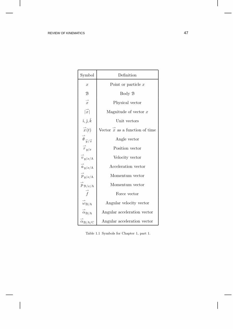
Symbol Definition
x Point or particle x
B Body B
x Physical vector
|x | Magnitude of vector x
ı, , k Unit vectors
x(t) Vector
x as a function of time
θy /
x
Angle vector
r y/x Position vector
v y/x/A Velocity vector
a y/x/A Acceleration vector
p y/x/A Momentum vector
pB/x/A Momentum vector
f Force vector
ωB/A Angular velocity vector
αB/A Angular acceleration vector
αB/A/C Angular acceleration vector
Table 1.1 Symbols for Chapter 1, part 1.

48 CHAPTER 1
Symbol Definition
ı, , k Cartesian frame
FA Frame A
er, eθ, k Cylindrical frame
er, eθ, eφ Spherical frame
et, en, eb Normal-tangential-binormal frame
eLV, eLH, eLN Local vertical/local horizontal frame
RA/B Rotation from FB to FA
RTA/B Rotation transpose, RB/A
OA/B Orientation of FA with respect to FB
OTA/B Orientation transpose, OB/A
R2(BΘ→ C) Orientation of FC with respect to FB given
by a rotation of FB about B by the angle Θ
3-2-1 rotation: Ψ,Θ,Φ Yaw, pitch, and roll angles
3-1-3 rotation: Φ,Θ,Ψ Precession, nutation, and spin angles
3-1-3 rotation: Ω, i, ω Orbital Euler angles
Table 1.2 Symbols for Chapter 1, part 2.

Chapter Two
Aircraft Kinematics
2.1 Frames Used in Aircraft Dynamics
To describe aircraft flight dynamics we consider four frames, namely,the Earth frame, aircraft frame, stability frame, and wind frame. The air-craft has six degrees of freedom, specifically, three translational degrees offreedom and three rotational degrees of freedom.
Translational Rotational
x: Surge Ψ: Yawy: Sway Θ: Pitchz: Plunge Φ: Roll
Longitudinal Lateral
x: Surge Ψ: YawΘ: Pitch y: Swayz: Plunge Φ: Roll
Table 2.1 Aircraft degrees of freedom using 3-2-1 Euler angles
Since a single degree of freedom is modeled by a second-order differ-ential equation, the dynamics of a six-degree-of-freedom rigid body suchas an aircraft are described by 6 second-order differential equations or 12first-order differential equations. For simplicity, we assume throughout thatthe velocity of the air with respect to the Earth is zero, that is, there is noambient wind.
2.1.1 Earth Frame FE
The Earth frame is assumed to be an inertial frame as explained inChapter 3. The origin OE of the Earth frame is any convenient point onthe Earth. The axes ıE and E are horizontal, while the axis kE pointsdownward.
The acceleration due to gravity is the physical acceleration vectorg = gkE, (2.1.1)

50 CHAPTER 2
?kE
9ıE
jE
OE
Figure 2.1.1The Earth frame FE.
where g = 9.8 m/s2. For a falling particle x,g is given by
g =
ax/OE/E. (2.1.2)
2.1.2 Aircraft Frame FAC
The aircraft frame is fixed to (painted on) the body of the aircraft andhas the origin OAC placed at the center of mass of the aircraft. The frameorigin OAC, along with the frame vectors ıAC and kAC, are chosen to lie inthe aircraft plane of symmetry.
Vectors in the aircraft frame are resolved as
r =r∣∣∣AC
.
We letr AC
=rOAC/OE
(2.1.3)
denote the location of the aircraft with respect to the origin of the Earthframe.
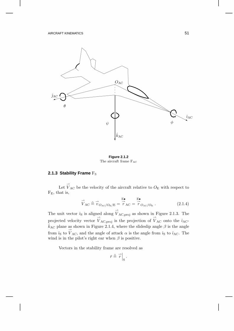
AIRCRAFT KINEMATICS 51
?kAC
ψ
*
9AC
θ
?
jıAC
φ
OAC
Figure 2.1.2The aircraft frame FAC
2.1.3 Stability Frame FS
LetV AC be the velocity of the aircraft relative to OE with respect to
FE, that is,
V AC
=vOAC/OE/E =
E•
r AC =
E•
r OAC/OE
. (2.1.4)
The unit vector ıS is aligned alongV AC,proj as shown in Figure 2.1.3. The
projected velocity vectorV AC,proj is the projection of
V AC onto the ıAC-
kAC plane as shown in Figure 2.1.4, where the slideslip angle β is the angle
from ıS toV AC, and the angle of attack α is the angle from ıS to ıAC. The
wind is in the pilot’s right ear when β is positive.
Vectors in the stability frame are resolved as
r =r∣∣∣S.

52 CHAPTER 2
?kAC
-ıAC
zıSz
V AC,proj
S = AC
kS
6α
-
α
Figure 2.1.3Rotation from the stability frame FS to the aircraft frame FAC.
Note that
OTS/AC = R
T2 (AC
−α→ S) = R2(Sα→ AC) = OAC/S.
2.1.4 Wind Frame FW
In the wind frame, the unit vector ıW points along the velocity vectorV AC as shown in Figure 2.1.4. The stability frame is transformed to the windframe by means of a rotation through β about the kW axis. Consequently,
FEΨ−→3
FE′Θ−→2
FE′′Φ−→1
FAC−α−→2
FSβ−→3
FW. (2.1.5)
Hence,
OTS/W = R
T3 (W
−β→ S) = R3(Sβ→ W) = OW/S.
2.2 Velocity Vector
The velocity of the aircraft with respect to the Earth is represented
byV AC. Letting U , V , and W be the components of
V AC in the aircraft

AIRCRAFT KINEMATICS 53
?S
-ıS - V AC,proj
zV AC
zıW
W
kS = kW
?β
β
Figure 2.1.4
Rotation from the wind frame FW to the stability frame FS and the projection of
V AC
onto ıS.
frame, we haveV AC = UıAC + V AC +WkAC,
and thusV AC resolved in the aircraft frame is
V AC
∣∣∣∣AC
=
UVW
. (2.2.1)
Letting US, VS, and WS be the components ofV AC in the stability frame,
we haveV AC = USıS + VSS +WSkS,
and thus
V AC
∣∣∣∣S
=
US
VS
WS
. (2.2.2)
The airspeed VAC is given by
VAC= |
V AC| =
√
U2 + V 2 +W 2 =√
U2S + V 2
S +W 2S .

54 CHAPTER 2
It can be seen from Figure 2.1.3 that
ıAC = (cosα)ıS − (sinα)kS,
AC = S,
kAC = (sinα)ıS + (cosα)kS,
which can be written as
ıAC
AC
kAC
=
cosα 0 − sinα0 1 0
sinα 0 cosα
︸ ︷︷ ︸
OAC/S=R2(Sα→AC)
ıSSkS
. (2.2.3)
Hence,
UVW
= R2(Sα→ AC)
US
VS
WS
. (2.2.4)
Since ıS is aligned alongV AC,proj, it follows that WS = 0. Then,
UVW
=
cosα 0 − sinα0 1 0
sinα 0 cosα
US
VS
0
, (2.2.5)
which yields
U = US cosα, (2.2.6)
V = VS, (2.2.7)
W = US sinα. (2.2.8)
Hence
tanα =W
U(2.2.9)
and
US =√
U2 +W 2. (2.2.10)
Furthermore,
sinα =W√
U2 +W 2(2.2.11)
and
cosα =U√
U2 +W 2. (2.2.12)

AIRCRAFT KINEMATICS 55
WkS
UkAC
*ıAC
::
ıS
V AC
6γOα
:
α
O
Θ horizontalS = AC
Figure 2.2.5Flight path angle γ and pitch angle Θ. In this figure, the angle of attack α is positive.
Note that Θ = α + γ.
The reverse of (2.2.4) is
US
VS
WS
= OS/AC
UVW
= R2(AC−α→ S)
UVW
=
cosα 0 sinα0 1 0
− sinα 0 cosα
UVW
. (2.2.13)
We define the flight path angle γ as the angle from the horizontal to ıSas shown in the Figure 2.2.5 and Figure 2.2.6. When the roll angle Φ = 0,the pitch angle of the aircraft is given by
Θ = α+ γ, (2.2.14)
which is the angle from the horizontal to ıAC.
Now, consider the wind frame FW, and recall that the aircraft velocity

56 CHAPTER 2
WkAC
UkS
: ıAC
*
*
ıS
V AC
6γO−α
:
−α
O
Θ horizontalS = AC
Figure 2.2.6Flight path angle γ and pitch angle Θ. In this figure, the angle of attack α is negative.
Note that Θ = α + γ.
V AC is aligned along ıW. From (2.1.5) we know that
V AC
∣∣∣∣W
= OW/S
V AC
∣∣∣∣S
= R3(Sβ→ W)
V AC
∣∣∣∣S
,
which can be written asV AC
∣∣∣∣S
= OS/W
V AC
∣∣∣∣W
= R3(W−β→ S)
V AC
∣∣∣∣W
.
Hence,
US
VS
0
=
cos β − sinβ 0sin β cos β 0
0 0 1
︸ ︷︷ ︸
OS/W=R3(W−β→S)
VAC
00
. (2.2.15)
Therefore,
US = VAC cos β (2.2.16)
and
VS = V = VAC sin β. (2.2.17)

AIRCRAFT KINEMATICS 57
Combining (2.2.5) and (2.2.15) we obtain
UVW
=
cosα 0 − sinα0 1 0
sinα 0 cosα
cos β − sin β 0sin β cos β 0
0 0 1
VAC
00
=
(cosα) cos β −(cosα) sin β − sinαsin β cos β 0
(sinα) cos β −(sinα) sin β cosα
VAC
00
=
(cosα) cos βsin β
(sinα) cos β
VAC. (2.2.18)
2.3 Rotational Kinematics
We now form a transformation matrix from FE to FAC using the yaw,pitch, and roll angles Ψ, Θ, and Φ as the 3-2-1 Euler angles. Note that yawis a rotation about the kE-axis, pitch is a rotation about the ′E-axis, androll is a rotation about the ı′′E-axis. Transformation from FE to FAC involvestwo intermediate frames, namely, FE′ and FE′′
The orientation matrices corresponding to the three rotations are givenby
OE′/E = R3(EΨ→ E′) =
cos Ψ sin Ψ 0− sin Ψ cos Ψ 0
0 0 1
, (2.3.1)
OE′′/E′ = R2(E′ Θ→ E′′) =
cos Θ 0 − sinΘ0 1 0
sinΘ 0 cos Θ
, (2.3.2)
and
OAC/E′′ = R1(E′′ Φ→ AC) =
1 0 00 cos Φ sin Φ0 − sinΦ cos Φ
.
The overall transformation can be represented as
FEΨ−→3
FE′Θ−→2
FE′′Φ−→1
FAC. (2.3.3)
58 CHAPTER 2
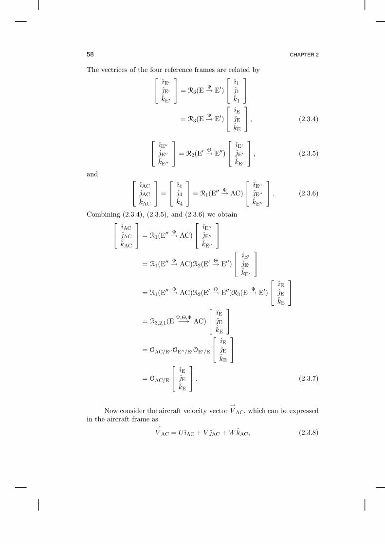
The vectrices of the four reference frames are related by
ıE′
E′
kE′
= R3(EΨ→ E′)
ı11k1
= R3(EΨ→ E′)
ıEEkE
, (2.3.4)
ıE′′
E′′
kE′′
= R2(E′ Θ→ E′′)
ıE′
E′
kE′
, (2.3.5)
and
ıAC
AC
kAC
=
ı44k4
= R1(E′′ Φ→ AC)
ıE′′
E′′
kE′′
. (2.3.6)
Combining (2.3.4), (2.3.5), and (2.3.6) we obtain
ıAC
AC
kAC
= R1(E′′ Φ→ AC)
ıE′′
E′′
kE′′
= R1(E′′ Φ→ AC)R2(E
′ Θ→ E′′)
ıE′
E′
kE′
= R1(E′′ Φ→ AC)R2(E
′ Θ→ E′′)R3(EΨ→ E′)
ıEEkE
= R3,2,1(EΨ,Θ,Φ−→ AC)
ıEEkE
= OAC/E′′OE′′/E′OE′/E
ıEEkE
= OAC/E
ıEEkE
. (2.3.7)
Now consider the aircraft velocity vectorV AC, which can be expressed
in the aircraft frame asV AC = UıAC + V AC +WkAC, (2.3.8)

AIRCRAFT KINEMATICS 59
and in the Earth frame asV AC = UEıE + VEE +WEkE. (2.3.9)
Using (1.13.1) on resolving vectors through a change of frame, we have
V AC
∣∣∣∣AC
= O3,2,1(EΨ,Θ,Φ−→ AC)
V AC
∣∣∣∣E
. (2.3.10)
For angular velocities, using the rotation sequence 3-1-3 (precession-nutation-spin) Euler angles (see 1.18.3), the angular velocity of the aircraftrelative to the Earth frame is defined by
ωAC
=ωAC/E. (2.3.11)
We use the notation
ωAC
∣∣∣AC
=
PQR
. (2.3.12)
Therefore,
ωAC
∣∣∣AC
=ωAC/E′′ +
ωE′′/E′ +
ωE′/E
= ΨkAC + ΘıE′′ + ΦkE′
=
(sin Θ) sin Ψ cos Ψ 0(sin Θ) cos Ψ − sinΨ 0
cos Θ 0 1
Φ
Θ
Ψ
. (2.3.13)
For the sequence 3-2-1 (yaw-pitch-roll) Euler angles, (see 1.18.6), we write
ωAC
∣∣∣AC
= ΦıAC + ΘE′′ + ΨkE′
=
− sin Θ 0 1(cos Θ) sin Φ cos Φ 0(cos Θ) cos Φ − sinΦ 0
Ψ
Θ
Φ
. (2.3.14)
2.4 Vector Derivatives in Rotating Frames
Letr be a position vector. Then the transport theorem given by Fact
1.19.1 implies that
E•
r =
AC•
r +
ωAC ×
r .

60 CHAPTER 2
Note thatE•
ωAC =
AC•
ω AC +
ωAC ×
ωAC =AC•
ω AC,
that is, the angular acceleration of the aircraft relative to the Earth frameis the same as the angular acceleration of the aircraft relative to the aircraftframe. Now consider the linear acceleration
E••
r =
E•
︷︸︸︷
AC•
r +
E•
︷ ︸︸ ︷ωAC ×
r
=AC••
r +
αAC/E/E
=AC••
r +
ωAC ×
AC•
r +
E•
ωAC ×
r +ωAC ×
(AC•
r +
ωAC ×
r
)
=AC••
r + 2
ωAC ×
AC•
r
︸ ︷︷ ︸
aCor
+E•
ωAC ×
r︸ ︷︷ ︸
aang
+ωAC ×
(ωAC ×
r)
︸ ︷︷ ︸
acent
, (2.4.1)
where, as in (1.22.1), aCor, aang, and acent are the Coriolis acceleration,angular-acceleration acceleration, and centripetal acceleration, respectively.
2.5 Cross Product
The cross product, introduced in Section 1.3, of
ωAC
∣∣∣AC
=
PQR
(2.5.1)
and
r |AC =
r1r2r3
(2.5.2)
can be represented as
ωAC
∣∣∣AC
×r |AC = det
ıAC AC kAC
P Q Rr1 r2 r3
(2.5.3)
= (Qr3 −Rr2)ıAC − (Pr3 −Rr1)AC + (Pr2 −Qr1)kAC.

AIRCRAFT KINEMATICS 61
Defining
ωAC
∣∣∣
×
AC=
0 −R QR 0 −P−Q P 0
,
we have
(ωAC ×
r )∣∣∣AC
=ωAC
∣∣∣AC
× r∣∣∣AC
=ωAC
∣∣∣
×
AC
r∣∣∣AC
=
0 −R QR 0 −P−Q P 0
r1r2r3
. (2.5.4)
2.6 Problems
Problem 2.6.1 Resolve the velocity vectorV AC =
V AC/E = 72 m/s ıAC − 6.3 m/s AC − 43 m/s kAC
in the stability and wind frames.
Problem 2.6.2 An aircraft is flying with an angle of attack of 14 and
no sideslip. The airspeed |V AC| is 94 m/s. Resolve
V AC in the aircraft frame
and in the stability frame.
Problem 2.6.3 An aircraft is flying with an angle of attack of 10 and
a sideslip angle of −19. The airspeed |V AC| is 80 m/s. Resolve
V AC in the
aircraft, stability, and wind frames.
Problem 2.6.4 Resolve the gravity vectorg symbolically in the air-
craft and stability frames. Then, set Ψ = 22, Θ = 5, Φ = −24, and
α = −17, and compute the components ofg in the aircraft and stability
frames.
Problem 2.6.5 Consider the position vectorr = 6.2 m ıE − 14.1 m E + 65.2 m kE
(m = meter) and assume that the orientation of the aircraft frame withrespect to the Earth frame is given by the yaw, pitch, roll Euler angles
Ψ = 62, Θ = 7, Φ = −12. Then resolver in the aircraft frame. Check
your answer by comparing the magnitude ofr computed from
r resolved
in both frames.

62 CHAPTER 2
Problem 2.6.6 An aircraft is flying with velocityV AC, which is con-
stant with respect to the Earth frame. Its angle of attack is −13, sideslip
angle is 24, and airspeed |V AC| is 85 m/s. The aircraft then rolls about ıAC
by +23 while the velocity vector remains fixed with respect to the Earth
frame. Resolve the velocity vectorV AC in the aircraft frame after the roll
is complete, and determine the new angle of attack and sideslip.
Problem 2.6.7 Write a Matlab program (and include your code) thatimplements the transformation from Euler angle rates to angular velocitycomponents given in class. Next, derive and confirm the reverse transfor-mation
Ψ = (Q sin Φ +R cos Φ) sec Θ,
Θ = Q cos Φ −R sin Φ,
Φ = P +Q(sin Φ) tan Θ +R(cos Φ) tan Θ,
and write a Matlab program that implements it. Finally, let
(Ψ,Θ,Φ) = (14,−29,−52),
(Ψ, Θ, Φ) = (19 deg/sec,−7 deg/sec, 16 deg/sec),
and compute (P,Q,R). Then use the computed values of (P,Q,R) in thereverse transformation and compute (Ψ, Θ, Φ). Verify that you recover theoriginal values of (Ψ, Θ, Φ).

AIRCRAFT KINEMATICS 63
Symbol Definition
FE Earth Frame
ıE, E, kE Earth frame axes
FAC Aircraft frame
ıAC, AC, kAC Aircraft frame axes
V AC Velocity of the aircraft relative to FE,
vOAC/OE/E
β Sideslip angle from ıS to ıW
FS Stability frame
ıS, S, kS Stability frame axes
r Component of a physical vector resolved in FS
FW Wind frame
ıW, W, kW Wind frame axes
U, V,W Components ofV AC resolved in FAC
US, VS,WS Components ofV AC resolved in FS
α Angle of attack angle from ıS to ıAC
γ Flight path angle from the horizontal to ıS
Θ Pitch angle from the horizontal to ıAC
ωAC Angular velocity of aircraft relative to FE,
ωAC/E
P,Q,R Components ofωAC resolved in FAC
aCor Coriolis acceleration
aang Angular-acceleration acceleration
acent Centripetal acceleration
Table 2.2 Symbols for Chapter 2.


Chapter Three
Review of Dynamics
Forces and moments can be applied to particles and bodies. Newton’s lawsrelate forces and moments to changes in momentum and angular momen-tum, respectively. These laws are axioms rather than provable mathematicalresults.
3.1 Newton’s First Law for Particles
We do not define the notion of a force, but rather we accept force asan intuitive notion and use it to define the concept of an inertial frame.
An unforced particle is a particle that has no forces acting on it.
The following result is Newton’s first law.
Fact 3.1.1 There exists a frame FA, called an inertial frame, suchthat, for all unforced particles x and y,
A••
r y/x = 0. (3.1.1)
Note that (3.1.1) can be written asa y/x/A. The origin OA of the
inertial frame FA is often taken to be the location of an unforced particle x.Note, however, that OA plays no role in this definition.
Fact 3.1.2 Let FA be an inertial frame, and let FB be a frame. Then
FB is an inertial frame if and only ifωB/A = 0.
Proof Use the double transport theorem Fact 1.20.1. Sufficiency isimmediate. Necessity is a little harder. Prove this result.
Fact 3.1.3 Let FA and FB be inertial frames. Then, for every physical

66 CHAPTER 3
vectorx(t),
A•
x (t) =
B•
x (t). (3.1.2)
3.2 Newton’s Second Law for Particles
Fact 3.2.1 Let FA be an inertial frame, let y be a particle with mass
m, letf y be a force acting on y, and let x be an unforced particle. Then,
mA••
r y/x =
f y. (3.2.1)
Fact 3.2.2 Let FA and FB be inertial frames, let y be a particle, letf y be a force acting on y, and let x be an unforced particle. Then,
A••
r y/x =
B••
r y/x. (3.2.2)
Proof Use (3.2.1) or double transport with Fact 3.1.2.
3.3 Forces and Moments
Let y be a particle in a body B, let w be a point, and letf y be a force
applied to y. Then the momentMy/w applied to y relative to w is defined
byMy/w
=r y/w ×
f y. (3.3.1)
Note that the point w may or may not be in the body B. See Fig. 3.3.1.
Let B be a body composed of particles m1, . . . ,ml, and letfmi
be a
force applied to mi. Then the net forcefB applied to B is defined by
f B
=
l∑
i=1
fmi
. (3.3.2)
Let B be a body composed of l rigidly interconnected particles m1, . . . ,
ml, let w be a point, and letfmi
be a force applied to mi. Then the net

REVIEW OF DYNAMICS 67
B
y
r
f
w
y/w
y
Figure 3.3.1
Representation of the moment
My/w =r y/w ×
f y relative to the point w due to the
force
f y applied to the particle y in the body B.
momentMB/w applied to B relative to w is defined by
MB/w
=
l∑
i=1
Mmi/w =
l∑
i=1
rmi/w ×
fmi
. (3.3.3)
Then net momentMB/w is a torque if the net force
fB is zero.
Fact 3.3.1 Let B be a body, letf x and
f y be forces applied to particles
x and y in B, respectively, assume thatf y = −
f x, and let w be a point.
Then the net moment applied to B relative to w isMB/w =
r x/y ×
f x. (3.3.4)

68 CHAPTER 3
Proof Note thatMB/w =
r x/w ×
f x +
r y/w × (−
f x)
=r x/w ×
f x +
r w/y ×
f x
=(r x/w +
r w/y
)
×f x
=r x/y ×
f x.
Note that the net force in Fact 3.3.1 is zero, and thus (3.3.4) is a
torque. Furthermore, the net momentMB/w in (3.3.4) is independent of w,
and is equivalent to the moment applied to x relative to y due to the forcef x applied to x. For the case of l particles, we have the following extension.
Fact 3.3.2 Let B be a body, and assume that the net force appliedto the body is zero. Then, the net moment applied to the body due to theforces is independent of the point relative to which the moment is taken.
3.4 Change in Angular Momentum
Let FA be an inertial frame, let B be a body composed of l intercon-nected particles m1, . . . ,ml, and let w be an unforced particle, as shown inFig. 3.4.2. We let mi denote both the name and the mass of the ith particle.Define the angular momentum of mi relative to w with respect to FA as
Hmi/w/A
=rmi/w ×mi
vmi/w/A, (3.4.1)
and, as in (1.16.3), define the angular momentum of B as
HB/w/A
=l∑
i=1
Hmi/w/A. (3.4.2)
Fact 3.4.1 Let FA be an inertial frame, let w be an unforced particle,let B be a body composed of l interconnected particles whose masses are
m1, . . . ,ml, respectively, and letfmi
be an external force applied to mi.Then
A•
HB/w/A =
MB/w, (3.4.3)
where
MB/w
=
l∑
i=1
rmi/w ×
fmi
. (3.4.4)

REVIEW OF DYNAMICS 69
f
y
i
j
ij
ji
iy /w
m
f
m
f
r
wi
Figure 3.4.2Body B composed of rigidly interconnected particles.
Proof Since mi and mj are rigidly connected, letf ij denote the con-
straint force on mi due to the connection to mj. Note thatf ij = −
f ji and
f ii = 0.
The moment applied to mi relative to w is given by
Mmi/w
=rmi/w ×
fmi
+l∑
j=1
f ij
.

70 CHAPTER 3
The change in angular momentum with respect to FA is thus given by
A•
Hmi/w/A =
A•
r mi/w ×mi
vmi/w/A +
rmi/w ×mi
A•
v mi/w/A
=vmi/w/A ×mi
vmi/w/A +
rmi/w ×mi
A•
v mi/w/A
=rmi/w ×mi
A•
v mi/w/A
=rmi/w ×mi
A••
r mi/w
=rmi/w ×
fmi
+
l∑
j=1
f ij
.
Hence,
A•
Hmi/w/A =
Mmi/w.
Summing over the particles m1, . . . ,ml yields
A•
HB/w/A =
l∑
i=1
A•
Hmi/w/A
=
l∑
i=1
Mmi/w
=
l∑
i=1
rmi/w ×
fmi
+
l∑
i,j=1,...,l
i6=j
rmi/w ×
f ij
=MB/w +
l∑
i,j=1,...,l
i<j
(rmi/w −
rmj/w
)
×f ij
=MB/w +
l∑
i,j=1,...,l
i<j
rmi/mj
×f ij
=MB/w,
where we used the fact thatf ij = −
f ji, as well as the fact that
rmi/mj
is
parallel tof ij.
The following result introduces the physical inertia matrix
I B/w of B
relative to w.

REVIEW OF DYNAMICS 71
Fact 3.4.2 Let B be a body with body-fixed frame FB, let FA be aframe, and let w be a point that is fixed in B. Then
HB/w/A =
I B/w
ωB/A, (3.4.5)
whereI B/w
=
l∑
i=1
mi
(∣∣∣rmi/w
∣∣∣
2U −
rmi/wrmi/w
)
. (3.4.6)
Furthermore,
I B/w
∣∣∣∣∣B
=
Ixx −Ixy −Ixz−Ixy Iyy −Iyz−Ixz −Iyz Izz
, (3.4.7)
where
Ixx
=
l∑
i=1
mi(y2i + z2
i ), Ixy
=
l∑
i=1
mixiyi,
Iyy
=
l∑
i=1
mi(x2i + z2
i ), Ixz
=
l∑
i=1
mixizi,
Izz
=
l∑
i=1
mi(x2i + y2
i )
︸ ︷︷ ︸
moments of inertia
, Iyz
=
l∑
i=1
miyizi
︸ ︷︷ ︸
products of inertia
. (3.4.8)
Proof Use (3.4.1) and the transport theorem to obtain
Hmi/w/A =
rmi/w ×mi
(B•
r mi/w +
ωB/A ×
rmi/w
)
,
whereB•
r mi/w is the velocity of the particle mi relative to w with respect to
FB. Since the particle mi is fixed in B relative to w, we haveB•
r mi/w = 0 for
all i = 0, . . . , l, and henceHmi/w/A =
rmi/w ×mi
(ωB/A ×
rmi/w
)
.
Summing over the l particles in the body yields
HB/w/A =
l∑
i=1
Hmi/w/A
=l∑
i=1
rmi/w ×mi
(ωB/A ×
rmi/w
)
.

72 CHAPTER 3
Next using (1.5.9) it follows that
HB/w/A =
l∑
i=1
mirmi/w ×
(ωB/A ×
rmi/w
)
=
l∑
i=1
mi
[(rmi/w ·rmi/w
)ωB/A −
(rmi/w ·ωB/A
)rmi/w
]
=
l∑
i=1
mi
[∣∣∣rmi/w
∣∣∣
2U −
rmi/wrmi/w
]
ωB/A
=
I B/w
ωB/A,
which proves (3.4.5). ResolvingHB/w/A in FB yields
HB/w/A
∣∣∣∣B
=
I B/w
∣∣∣∣∣B
ωB/A
∣∣∣B
=l∑
i=1
mi
(∣∣∣rmi/w
∣∣∣
2I3 −
rmi/w
∣∣∣B
rmi/w
∣∣∣
T
B
)
PQR
=l∑
i=1
mi
x2i + y2
i + z2i 0 0
0 x2i + y2
i + z2i 0
0 0 x2i + y2
i + z2i
−
x2i xiyi xizi
yixi y2i yizi
zixi ziyi z2i
PQR
, (3.4.9)
wherermi/w = xiıB + yiB + zikB
andωB/A = P ıB +QB +RkB.
Hence
I B/w
∣∣∣∣∣B
is given by (3.4.7) and (3.4.8).
Fact 3.4.3 Let FA be an inertial frame, let B be a body, and let FB
be a body-fixed frame. Then,I B/w
B•
ω B/A +
ωB/A ×
I B/w
ωB/A =
MB/w. (3.4.10)

REVIEW OF DYNAMICS 73
Proof Combining (3.4.3) and (3.4.5) yields
A•
HB/w/A =
A•
︷ ︸︸ ︷I B/w
ωB/A =
MB/w, (3.4.11)
where the net momentMB/w on B relative to w is given by (3.4.4). Next,
the transport theorem and (3.4.5) yield
A•
HB/w/A =
B•
HB/w/A +
ωB/A ×
HB/w/A
=
B•
︷ ︸︸ ︷I B/w
ωB/A +
ωB/A ×
I B/w
ωB/A. (3.4.12)
Since the locations of the mass particles of B do not change relative to B,we have
B•
︷ ︸︸ ︷I B/w
ωB/A =
I B/w
B•
ω B/A . (3.4.13)
Combining (3.4.3), (3.4.12), and (3.4.13), yields (3.4.10).
Fact 3.4.4 Let B be a body, let w be a point, let
I B/w be given by
(3.6.1), let
R be a physical rotation matrix, and let
I
′
B/w be the physical
inertia matrix of
RB. Then
I
′
B/w =
R
I B/w
R
T
. (3.4.14)
Fact 3.4.5 Let B be a body with body-fixed frame FB, let w be a
point, let
I B/w be the physical inertia matrix of B, and let FA be a frame.
ThenI B/w
∣∣∣∣∣A
= OA/B
I B/w
∣∣∣∣∣B
OB/A. (3.4.15)
Proof The result follows from Fact 1.10.10.

74 CHAPTER 3
3.5 Momentum and Angular Momentum Relative toCenter of Mass
Note that the center of mass c of a body B composed of rigidly inter-connected particles m1, . . . ,ml whose masses are m1, . . . ,ml, respectively,satisfies
l∑
i=1
mirmi/c = 0. (3.5.1)
Fact 3.5.1 Let B be a body composed of rigidly interconnected parti-cles m1, . . . ,ml whose masses are m1, . . . ,ml, respectively, let c denote the
center of mass of B, letfmi
be an external force applied to the particle mi,assume that B is subject to gravity, let FA be an inertial frame, and let wbe an unforced particle. Then
A•
p B/w/A=
f B, (3.5.2)
where
fB
=l∑
i=1
(fmi
+mig ). (3.5.3)
Proof Note that
A•
p B/w/A =
l∑
i=1
mi
A•
v mi/w/A
=l∑
i=1
(fmi
+mig )
=fB.
The following result shows that gravity does not contribute to the netmoment on a rigid body relative to its center of mass.
Fact 3.5.2 Let B be a body composed of rigidly interconnected parti-cles m1, . . . ,ml whose masses are m1, . . . ,ml, respectively, let c denote thecenter of mass of B, assume that B is subject to gravity, and, for i = 1, . . . , l,
letfmi
be an additional external force applied to the particle mi. Then
MB/c =
l∑
i=1
rmi/c ×
fmi
. (3.5.4)

REVIEW OF DYNAMICS 75
Proof Using (3.5.1) it follows that
MB/c =
l∑
i=1
rmi/c × (
fmi
+mig )
=
l∑
i=1
rmi/c ×
fmi
+
l∑
i=1
rmi/c ×mi
g
=
l∑
i=1
rmi/c ×
fmi
+
(l∑
i=1
mirmi/c
)
×g
=
l∑
i=1
rmi/c ×
fmi
.
Fact 3.5.3 Let B be a body composed of rigidly interconnected parti-cles m1, . . . ,ml whose masses are m1, . . . ,ml, respectively, let c be the centerof mass of B, let mB
=∑l
i=1mi be the mass of B, let FA be an inertialframe, let w be an unforced particle, assume that B is subject to gravity, for
i = 1, . . . , l letfmi
be an additional external force applied to the particlemi, and define
Hc/w/A
=r c/w ×mB
A•
r c/w (3.5.5)
and
HB/c/A
=l∑
i=1
(
rmi/c ×mi
A•
r mi/c
)
. (3.5.6)
ThenHB/w/A =
HB/c/A +
Hc/w/A. (3.5.7)
Furthermore,
A•
HB/c/A =
MB/c (3.5.8)
andA•
H c/w/A =
M c/w, (3.5.9)
whereM c/w
=r c/w ×
fB, (3.5.10)
fB
=l∑
i=1
(fmi
+mig ), (3.5.11)

76 CHAPTER 3
and
MB/c
=
l∑
i=1
rmi/c ×
fmi
. (3.5.12)
Proof Since w is an unforced particle, it follows from (3.4.3) that
HB/w/A =
l∑
i=1
(rmi/c +
r c/w
)
×mi
(A•
r mi/c +
A•
r c/w
)
=r c/w ×mB
A•
r c/w +
r c/w ×
l∑
i=1
mi
A•
r mi/c
+
l∑
i=1
rmi/c ×mi
A•
r c/w +
l∑
i=1
rmi/c ×mi
A•
r mi/c . (3.5.13)
Since c is the center of mass of B, it follows from (3.5.1) that the secondand third terms in (3.5.13) are zero. Therefore,
HB/w/A =
r c/w ×mB
A•
r c/w +
l∑
i=1
rmi/c ×mi
A•
r mi/c,
which is equivalent to (3.5.7).
Note thatHc/w/A is the angular momentum of a particle of mass mB
relative to w with respect to FA, whereHB/c/A is the angular momentum
of B relative to its center of mass c with respect to FA.
Next, differentiating (3.5.7) yields
A•
HB/w/A =
A•
H c/w/A +
A•
HB/c/A, (3.5.14)
whereA•
H c/w/A
=r c/w ×mB
A••
r c/w (3.5.15)
andA•
HB/c/A =
l∑
i=1
rmi/c ×mi
A••
r mi/c . (3.5.16)
Now it follows from Fact 3.5.1 that
fB = mB
A••
r c/w, (3.5.17)

REVIEW OF DYNAMICS 77
wherefB is the net force acting on B. Hence it follows from (3.5.15) and
(3.5.17) that
A•
H c/w/A =
M c/w, (3.5.18)
whereM c/w
=r c/w ×
fB. (3.5.19)
Furthermore, note that
MB/w =
l∑
i=1
rmi/w ×
fmi
=
l∑
i=1
(rmi/c +
r c/w
)
×fmi
=l∑
i=1
rmi/c ×
fmi
+r c/w ×
f B
=l∑
i=1
rmi/c ×
fmi
+M c/w
=MB/c +
M c/w. (3.5.20)
Therefore, it follows from (3.5.20) and (3.5.12) that
MB/c +
M c/w =
MB/w
=
A•
HB/w/A
=
A•
H c/w/A +
A•
HB/c/A
=M c/w +
A•
HB/c/A .
Hence (3.5.8) holds.
3.6 Continuum Bodies
Replacing finite sums with integrals, IB/w is given by the followingresult.

78 CHAPTER 3
Fact 3.6.1 Let B be a body and let w be a point. ThenI B/w =
∫
B
∣∣∣r dm/w
∣∣∣
2U −
r dm/wr dm/w dm. (3.6.1)
Furthermore,
IB/w=
I B/w
∣∣∣∣∣B
=
Ixx −Ixy −Ixz−Iyx Iyy −Iyz−Izx −Izy Izz
, (3.6.2)
where
Ixx=
∫
B
(y2 + z2
)dm, Ixy
=
∫
B
xy dm,
Iyy
=
∫
B
(x2 + z2
)dm, Ixz
=
∫
B
xz dm,
Izz
=
∫
B
(x2 + y2
)dm
︸ ︷︷ ︸
moments of inertia
, Iyz
=
∫
B
yz dm
︸ ︷︷ ︸
products of inertia
.
To be added: Center of mass for a continuum body
3.7 Properties of the Inertia Matrix
Every rigid body B has an inertia dyadic
I B/w, which can be resolved
in a body-fixed frame FB to obtain
IB/w=
I B/w
∣∣∣∣∣B
=
Ixx −Ixy −Ixz−Ixy Iyy −Iyz−Ixz −Iyz Izz
.
The inertia matrix measures the mass distribution with respect to the chosencoordinate frame. The inertia matrix has the following properties:
• IB/w is symmetric and positive definite, which implies that all of theeigenvalues of the inertia matrix are positive.
• The eigenvalues λ1 ≥ λ2 ≥ λ3 of IB/w satisfy
λ1 < λ2 + λ3,
that is, the eigenvalues satisfy the triangle rule.

REVIEW OF DYNAMICS 79
• If IB/w is diagonal, that is,
IB/w =
λ1 0 00 λ2 00 0 λ3
, (3.7.1)
then the coordinate axes of FB are the principal axes, and λ1, λ2, λ3
are the principal moments of inertia.
• If the inertia matrix is not diagonal, then there exists a frame withrespect to which the resolved inertia tensor is diagonal. Equivalently,there exists a proper orthogonal matrix S such that SIST is diagonal.
Example 3.7.1 The inertia matrix for a sphere has the form
IB/c =
λ 0 00 λ 00 0 λ
, (3.7.2)
that is, λ1 = λ2 = λ3.
Example 3.7.2 The inertia matrix for a cube is the same as that of asphere.
Example 3.7.3 The inertia matrix of a rectangular prism is of theform
IB/c =
λ1 0 00 λ2 00 0 λ3
, (3.7.3)
where the axes of FB are chosen to be perpendicular to the sides of the box.
Example 3.7.4 Two of the three moments of inertia are equal for acylinder, in particular, λ1 = λ2 > λ3.
3.8 Problems
Problem 3.8.1 Assuming the symmetry of a typical aircraft, showthat 4 of the entries of the inertia tensor resolved in the aircraft frame arezero. Next, write out the entries of the inertia tensor resolved in the stabilityframe in terms of the entries of the inertia tensor resolved in the aircraftframe.
Problem 3.8.2 Explain why the inertia matrix of a homogeneous cubeis independent of the frame you choose for resolving the inertia tensor.
Problem 3.8.3 Consider a rigid body spinning about a principal axis

80 CHAPTER 3
Symbol Definition
c Center of mass of B
dm Mass element of B
I B/w Physical inertia matrix of body B relative to w
λ Eigenvalue of the inertia matrix
HB/w/A Angular momentum vectorMB/y Net moment vector
Table 3.1 Symbols for Chapter 3.
and unperturbed by any applied moments. Use Euler’s equation to showthat the body will spin indefinitely about the principal axis.

Chapter Four
Aircraft Dynamics
4.1 Flight Dynamics and Control
From a dynamics and control point of view, there are two main re-quirements for an aircraft. An aircraft needs to be 1) stable so that it canmaintain course despite disturbances, and 2) controllable so that it can bemaneuvered. A challenge arises due to the fact that stability and control-lability of an aircraft are conflicting requirements. Forces and moments areneeded for control.
4.2 History of Aircraft Stability and Control
• Cayley - Oar with cruciform tail
• Lanchester - Wing dihedral (gliders).
• Bryon - Analyzed linearized flight.
4.3 Aerodynamic Forces
The net aerodynamic forceFA on the center of mass OAC of the air-
craft is given byFA =
D +
L, (4.3.1)
whereD = −DıW (4.3.2)
andL
= −LkW (4.3.3)

82 CHAPTER 4
are the drag and lift vectors, respectively, andD and L are positive numbers.Hence,
FA = −DıW − LkW. (4.3.4)
Note that the direction of the drag vectorD is opposite to the velocity
vectorV AC, and thus is in the direction of the wind relative to the aircraft.
Furthermore, the lift forceL is normal to
V AC and lies in the plane of
symmetry of the aircraft. We usually ignore the contribution of the controlsurfaces to the net aerodynamic force.
We can writeFA as
FA =
FAx
+FAy
+FAz
,
whereFAx
,FAy
, andFAz
are the frontal, side, and downward forces on the
aircraft in the directions ıS, S, and kS, respectively. Hence,D =
FAx
+FAy
(4.3.5)
andL =
FAz
. (4.3.6)
The frontal forceFAx
is given by
FAx
= FAx
V AC
|V AC|
= FAxıS. (4.3.7)
Hence, FAxis a negative number. Furthermore, the side force
FAy
is givenby
FAy
= FAyAC = FAy
S. (4.3.8)
Note that FAy> 0 denotes a left-to-right force, which corresponds to β < 0.
Finally, since kW = kS, the liftL is given by
L = −LkS = FAz
kS = −LkW = FAzkW. (4.3.9)
Hence, we haveFA = FAx
ıS + FAyS − LkS,

AIRCRAFT DYNAMICS 83
?kS = kW
6
L =
FAz
W
:ıAC
WkAC
FAx
i
D
-ıS
-V AC,proj
K α
qV AC
qıW
β
FAy
Figure 4.3.1
Aerodynamic forces. The vectors ıW and W point obliquely out of the page, while
D
points obliquely into the page.
and thus
FA
∣∣∣∣S
=
FAx
FAy
FAx
=
−D cosβ−D sinβ
−L
= OS/W
FA
∣∣∣∣W
=
cos β − sin β 0sin β cos β 0
0 0 1
−D0−L
.
Note that
D =√
F 2Ax
+ F 2Ay. (4.3.10)
4.4 Translational Momentum Equations
Recall thatr AC
=rOAC/OE
(4.4.1)
denotes the location of the center of mass of the aircraft with respect to theorigin of FE, which is assumed for convenience to be an unforced particle,
and define the velocityV AC of the aircraft relative to the Earth with respect

84 CHAPTER 4
to the Earth frame by
V AC
=vOAC/OE/E =
E•
r AC =
E•
r OAC/OE/E . (4.4.2)
Then,
m
E•
V AC = m
g +
FA +
FT, (4.4.3)
whereFT is the engine thrust force. Using the transport theorem (1.19) to
introduce the derivative with respect to the aircraft frame FAC into (4.4.3)yields
m
AC•
V AC +
ωAC ×
V AC
= mg +
FA +
FT, (4.4.4)
whereωAC =
ωAC/E. Resolving (4.4.4) in the aircraft frame yields
m
AC•
V AC
∣∣∣∣∣∣AC
+ (ωAC ×
V AC)
∣∣∣∣AC
= mg∣∣∣AC
+FA
∣∣∣∣AC
+FT
∣∣∣∣AC
.
(4.4.5)
Note that
ωAC
∣∣∣AC
=
PQR
. (4.4.6)
Resolving the gravity vector in the Earth frame asg = gkE yields
g∣∣∣E
=
00g
.

AIRCRAFT DYNAMICS 85
Transforming to the aircraft frame yields
g∣∣∣AC
= R3,2,1(EΨ,Θ,Φ−→ AC)
00g
= R1(E′′ Φ→ AC)R2(E
′ Θ→ E′′)R3(EΨ→ E′)
00g
=
[1 0 00 cos Φ sinΦ0 − sin Φ cos Φ
] [cos Θ 0 − sin Θ
0 1 0sin Θ 0 cos Θ
] [cos Ψ sinΨ 0− sin Ψ cos Ψ 0
0 0 1
] [00g
]
=
−g sin Θg(sin Φ) cos Θg(cos Φ) cos Θ
. (4.4.7)
Hence, we define
gxgygz
=
−g sin Θg(sin Φ) cos Θg(cos Φ) cos Θ
. (4.4.8)
Notice that the yaw angle Ψ does not appear ing∣∣∣AC
.
Next, consider the aerodynamic forceFA resolved in the stability
frame
FA
∣∣∣∣S
=
FAx
FAy
FAz
=
−D cos β−D sin β
−L
. (4.4.9)
These forces can be expressed in the aircraft frame by noting that
FA
∣∣∣∣AC
= R2(Sα→ AC)
−D cos β−D sin β
−L
=
cosα 0 − sinα0 1 0
sinα 0 cosα
−D cos β−D sin β
−L
=
−D(cos β) cosα+ L sinα−D sinβ
−D(cos β) sinα− L cosα
=
FAx
FAy
FAz
. (4.4.10)

86 CHAPTER 4
FT
*
rT
cg
V AC
KΦT
Figure 4.4.2Thrust force and engine geometry.
For the thrust force we express
FT
∣∣∣∣AC
=
FTx
FTy
FTz
=
cos ΦT 0 sin ΦT
0 1 0− sin ΦT 0 cos ΦT
FT
00
=
FT cos ΦT
0−FT sinΦT
, (4.4.11)
where FT is the engine force and ΦT is the angle from ıAC to the engineforce direction, shown in Fig. 4.4.2. We assume that the engine thrust hasa zero component in the AC direction.
Now, since
AC•
V AC =
AC•
︷ ︸︸ ︷(
UıAC + V AC +WkAC
)
= U ıAC + V AC + W kAC,
we have
AC•
V AC
∣∣∣∣∣∣AC
=
U
V
W
. (4.4.12)

AIRCRAFT DYNAMICS 87
Substituting (4.4.6), (4.4.8), (4.4.10), (4.4.11), and (4.4.12) into (4.4.5) weobtain the surge, sway, and plunge equations
m(
U − V R+WQ)
= mgx + FAx+ FTx
, (4.4.13)
m(
V + UR−WP)
= mgy + FAy, (4.4.14)
m(
W − UQ+ V P)
= mgz + FAz+ FTz
, (4.4.15)
or, equivalently,
m(
U − V R+WQ)
= −mg sin Θ −D(cos β) cosα+ L sinα+ FT cos ΦT,
(4.4.16)
m(
V + UR−WP)
= −D sinβ +mg(sin Φ) cos Θ, (4.4.17)
m(
W − UQ+ V P)
= mg(cos Φ) cos Θ−D(cos β) sinα
− L cosα− FT sin ΦT. (4.4.18)
4.5 Rotational Momentum Equations
LetωAC = P ıAC +QAC +RkAC (4.5.1)
be the angular velocity of the aircraft frame FAC with respect to the Earthframe FE. Let
HAC/E
=HAC/c/E (4.5.2)
denote the angular momentum of the aircraft relative to the center of massc
= OAC of the aircraft with respect to FE. Using (3.4.5) we have
HAC/E
∣∣∣∣AC
=
Hx
Hy
Hz
=
Ixx −Ixy −Ixz−Ixy Ixy −Iyz−Ixz −Iyz Izz
PQR
.
For most aircraft, AC-kAC is a plane of symmetry. Hence
Ixy =
∫
ACxy dm = 0 (4.5.3)
and
Iyz =
∫
ACyz dm = 0. (4.5.4)

88 CHAPTER 4
Consequently,
Hx = IxxP − IxzR, (4.5.5)
Hy = IyyQ, (4.5.6)
Hz = IzzR− IxzP. (4.5.7)
Next, Euler’s equation (3.4.10) for the aircraft is given by
I AC/c
AC•
ω AC +
ωAC ×
I AC/c
ωAC =
MAC/c, (4.5.8)
whereMAC/c
=MA/c +
MT/c (4.5.9)
is the net moment acting on the aircraft relative to c, andMA/c and
MT/c
are the aerodynamic and thrust moments relative to c, respectively. The netaerodynamic moment is produced by the air flow over both the fixed andvariable (control) surfaces of the aircraft.
In the aircraft frame, we have
MAC/c
∣∣∣∣AC
=
LAC
MAC
NAC
=MA/c
∣∣∣∣AC
+MT/c
∣∣∣∣AC
, (4.5.10)
where
MA/c
∣∣∣∣AC
=
LA
MA
NA
and
MT/c
∣∣∣∣AC
=
LT
MT
NT
.
Hence,
LAC
MAC
NAC
=
LA
MA
NA
+
LT
MT
NT
. (4.5.11)
Now resolving Euler’s equation (4.5.8) in the aircraft frame yields(I AC/c
AC•
ω AC
)∣∣∣∣∣AC
+
(
ωAC ×
I AC/c
ωAC
)∣∣∣∣∣AC
=MAC/c
∣∣∣∣AC
, (4.5.12)

AIRCRAFT DYNAMICS 89
which yields
IxxP − IxzR
IyyQ
IzzR− IxzP
+
0 −R QR 0 −P−Q P 0
IxxP − IxzRIyyQ
IzzR− IxzP
=
LAC
MAC
NAC
.
(4.5.13)
Equation (4.5.13) can now be written component-wise as the roll,pitch, and yaw equations
IxxP + (Izz − Iyy)QR− Ixz
(
R+ PQ)
= LAC, (4.5.14)
IyyQ+ (Ixx − Izz)PR+ Ixz(P 2 −R2
)= MAC, (4.5.15)
IzzR+ (Iyy − Ixx)PQ+ Ixz
(
QR− P)
= NAC. (4.5.16)
Equations (4.5.14), (4.5.15), and (4.5.16) are the roll, pitch, and yaw mo-ment equations, respectively. Each moment equation has three terms, eachrepresenting a physical effect. The first term is the angular accelerationterm, the next term is the gyroscopic precession term, and the last term isthe inertia coupling term. For the roll equation,
IxxP︸ ︷︷ ︸
angular acceleration
+ (Izz − Iyy)QR︸ ︷︷ ︸
gyroscopic precession
− Ixz
(
R+ PQ)
︸ ︷︷ ︸
inertial coupling
= LAC.
4.6 Aircraft Equations of Motion Resolved in FAC
Translational kinematics (see (2.2.1))
E•
r
∣∣∣∣∣AC
=VAC
∣∣∣∣AC
=
UVW
.
Rotational kinematics (see (2.3.14) and (2.3.12))
PQR
=
− sinΘ 0 1(cos Θ) sin Φ cos Φ 0(cos Θ) cos Φ − sin Φ 0
Ψ
Θ
Φ
.
Translational momentum (see (4.4.16), (4.4.17), and (4.4.18))
m(
U − V R+WQ)
= −mg sin Θ −D(cos β) cosα+ L sinα+ FT cos ΦT,
(4.6.1)
m(
V + UR−WP)
= −D sin β +mg(sin Φ) cos Θ, (4.6.2)

90 CHAPTER 4
m(
W − UQ+ V P)
= mg(cos Φ) cos Θ−D(cos β) sinα
− L cosα− FT sin ΦT.(4.6.3)
Rotational momentum (see (4.5.14), (4.5.15), and (4.5.16))
IxxP + (Izz − Iyy)QR− Ixz
(
R+ PQ)
= LAC = LA + LT, (4.6.4)
IyyQ+ (Ixx − Izz)PR+ Ixz(P 2 −R2
)= MAC = MA +MT, (4.6.5)
IzzR+ (Iyy − Ixx)PQ+ Ixz
(
QR− P)
= NAC = NA +NT. (4.6.6)
4.7 Problems
Problem 4.7.1 Resolve the aerodynamic force vectorFA symbolically
in the aircraft frame.
Problem 4.7.2 Consider Fig. 4.4.2. Determine
LT
MT
NT
in terms of ΦT and rT.

AIRCRAFT DYNAMICS 91
Symbol Definition
FA Aerodynamic force vector
D Drag force
FAxFrontal force in FS
FAySide force in FS
FAzVertical force in FS
L Lift force
FT Engine thrust force vector
FT Magnitude of the thrust force
ΦT Angle between the thrust force and ıSMAC Total moment vector on the aircraft
LAC Total roll moment on the aircraft
MAC Total pitch moment on the aircraft
NAC Total yaw moment on the aircraft
MA Aerodynamic moment vector
LA Aerodynamic roll moment in FAC
MA Aerodynamic pitch moment in FAC
NA Aerodynamic yaw moment in FAC
MT Thrust moment vector
LT Thrust roll moment in FAC
MT Thrust pitch moment in FAC
NT Thrust yaw moment in FACI AC/c Aircraft inertia tensor
Table 4.1 Symbols for Chapter 4, part 1.

92 CHAPTER 4
Symbol Definition
LAC Total roll moment in FS
MAC Total pitch moment in FS
NAC Total yaw moment in FS
LA Aerodynamic roll moment in FS
MA Aerodynamic pitch moment in FS
NA Aerodynamic yaw moment in FS
LT Thrust roll moment in FS
MT Thrust pitch moment in FS
NT Thrust yaw moment in FS
Table 4.2 Symbols for Chapter 4, part 2.

Chapter Five
Linearization
The goal of linearization is to approximate the nonlinear aircraft equationsof motion with linear equations to facilitate the analysis of flight character-istics in the vicinity of steady flight. The linearized equations are easier toanalyze than the original nonlinear equations and involve stability deriva-tives that can be estimated using computational fluid dynamics (CFD) codesor measured through experiments in a wind tunnel.
5.1 Taylor series
The Taylor series expansion of an infinitely differentiable func-tion f in a neighborhood of a is expressed as
f(x) = f(a) + f ′(a)(x− a) +f ′′(a)
2(x− a)2 +
f (3)(a)
3!(x− a)3 + · · ·
(5.1.1)
In a more compact form, we have
f(x) =
∞∑
i=0
f (i)(a)
i!(x− a)i. (5.1.2)
For a multivariable function, we write
f(x, y) = f(a, b) +∂f
∂x
∣∣∣∣(a,b)
(x− a) +∂f
∂y
∣∣∣∣(a,b)
(y − b)
+1
2
∂2f
∂x2
∣∣∣∣(a,b)
(x− a)2 +∂2f
∂x∂y
∣∣∣∣(a,b)
(x− a)(y − b)
+1
2
∂2f
∂y2
∣∣∣∣(a,b)
(y − b)2 + · · · . (5.1.3)
Truncating the series (5.1.3) to the first power in x and y yields the approx-

94 CHAPTER 5
imation
f(x, y) ≈f(a, b) +∂f
∂x
∣∣∣∣(a,b)
(x− a) +∂f
∂y
∣∣∣∣(a,b)
(y − b). (5.1.4)
Example 5.1.1 Consider the lift model
L(α, α, β, β, δe) = CL(α, α, β, β, δe)pdS,
where δe and pd are the elevator angle and dynamic pressure, respectively.Then
CL(α0 + δα, δα,β0 + δβ, δβ, δe)
≈ CL(α0, 0, 0, 0, 0)
+∂CL∂α
(α0, 0, 0, 0, 0)δα +∂CL∂δα
(α0, 0, 0, 0, 0)δα
+∂CL∂β
(α0, 0, 0, 0, 0)δβ +∂CL
∂β(α0, 0, 0, 0, 0)δβ
+∂CL∂δe
(α0, 0, 0, 0, 0)δe. (5.1.5)
5.2 Alternative Linearization Procedure
The following alternative procedure is sometimes simpler than usingthe Taylor expansion.
• Replace each variable with the sum of its steady-state value and aperturbation. For instance, U = U0 + u.
• Since the product of two small quantities is even smaller, ignore prod-ucts of perturbation variables.
• Subtract the nominal equation to delete all terms involving only thesteady-state values.
5.3 Trigonometric Functions
Using the Taylor expansion, we have
sin(Φ0 + φ) ≈ sinΦ0 + (cos Φ0)φ, (5.3.1)
cos(Φ0 + φ) ≈ cos Φ0 − (sin Φ0)φ. (5.3.2)

LINEARIZATION 95
Hence, for Φ0 = 0, we have the small-angle approximations
sinφ ≈ φ (5.3.3)
and
cosφ ≈ 1. (5.3.4)
Note that (5.3.1) and (5.3.2) can also be obtained from the trigonometricidentities
sin(Φ0 + φ) = (sin Φ0) cos φ+ (cos Φ0) sinφ (5.3.5)
and
cos(Φ0 + φ) = (cos Φ0) cosφ− (sin Φ0) sinφ. (5.3.6)
5.4 Steady Flight
Recall that
V AC =
vOAC/OE/E =
E•
r AC =
E•
r OAC/OE
. (5.4.1)
The conditions for steady flight are
AC•
V AC = 0 (5.4.2)
andAC•
ω AC = 0. (5.4.3)
These conditions mean that the velocity vectorV AC and the angular velocity
vectorωAC are constant with respect to the aircraft frame FAC. Under these
conditions, we denoteV AC and
ωAC by
V AC0
andωAC0
, respectively, where
V AC0
∣∣∣∣AC
=
U0
V0
W0
(5.4.4)
and
ωAC0
∣∣∣AC
=
P0
Q0
R0
. (5.4.5)
The aircraft can fly in several possible steady regimes, including
• Straight-line flight, either climb, level, or descent

96 CHAPTER 5
• Circular flight, which is banked or sideslipping
• Helical flight
Steady flight also includes hover as well as both rotation around andconstant-speed translation along any body axis. For example, rotation
around ıAC along withV AC = VACıAC constitutes steady flight known as a
barrel roll.
5.5 Linearization of the Aircraft Kinematics
We linearize the aircraft equations of motion about straight-line,constant-speed wings-level steady flight. Straight-line constant-speed flightmeans
U0 = constant, β0 = 0, Ψ0 = constant, Θ0 = α0 + γ0, (5.5.1)
while wings-level flight implies
Φ0 = 0, P0 = Q0 = R0 = 0. (5.5.2)
Here α0, β0, and γ0 denote the steady values of the angle of attack, sideslip,and flight path angles, respectively, while Ψ0, Θ0, and Φ0 denote steadyvalues of the 3-2-1 sequence of Euler rotations from FE to FAC. Note thatβ0 = 0 implies V0 = 0.
Next, consider the perturbed angular velocities
ωAC/E
∣∣∣AC
=
PQR
=
P0 + pQ0 + qR0 + r
=
pqr
, (5.5.3)
and the perturbed 3-2-1 Euler angles
ΨΘΦ
=
Ψ0 + ψΘ0 + θΦ0 + φ
=
Ψ0 + ψΘ0 + θφ
. (5.5.4)
It thus follows from (1.18.6) that
pqr
=
− sinΘ0 0 10 1 0
cos Θ0 0 0
ψ
θ
φ
. (5.5.5)

LINEARIZATION 97
?WAC
?kE
O
L
W kS
W
FAz
T
ΦTI*
V AC,proj
ıAC*
K α0:
V AC
: ıSγ0
K
-ıE
*
FAx
Figure 5.5.1Steady flight conditions. All vectors shown lie in the aircraft plane of symmetry.
5.6 Linearization of the Aircraft Dynamics in FAC
Consider the surge equation resolved in FAC given by
m(
U − V R+WQ)
= −mg sinΘ + FAx+ FTx
. (5.6.1)
At nominal flight conditions, (5.6.1) becomes
m(
U0 − V0R0 +W0Q0
)
= −mg sinΘ0 + FAx0+ FTx0
. (5.6.2)
Using (5.5.1), (5.5.2), and (5.6.2) yields
−mg sin Θ0 + FAx0+ FTx0
= 0. (5.6.3)
Now, replace each variable with the sum of its nominal value and a pertur-bation to obtain
m[
U0 + u− (V0 + v)(R0 + r) + (W0 + w)(Q0 + q)]
= −mg sin(Θ0 + θ) + FAx0+ fAx
+ FTx0+ fTx
.
(5.6.4)

98 CHAPTER 5
Substituting the nominal flight conditions (5.5.1) and (5.5.2) into (5.6.4)and using the trigonometric identity (5.3.5) yields
m(U0 + u− V0r −R0v − V0R0 − vr +W0Q0 +W0q +Q0w + wq)
= −mg[(sin Θ0) cos θ + (cos Θ0) sin θ] + FAx0+ fAx
+ FTx0+ fTx
.
(5.6.5)
Neglecting the products of perturbation variables and making small-angleapproximations for θ yields
m(U0 + u− V0r −R0v − V0R0 +W0Q0 +W0q +Q0w)
= −mg(sin Θ0 + θ cos Θ0) + FAx0+ fAx
+ FTx0+ fTx
.
(5.6.6)
Now substracting the nominal equation (5.6.3) from (5.6.6) yields the lin-earized surge equation
mu = −mW0q −mg(cos Θ0)θ + fAx+ fTx
, (5.6.7)
which is linear in terms of the perturbation variables u, q, and θ. Similarly,we have the linearized sway and plunge equations
mv = −mU0r +mW0p+mg(cos Θ0)φ+ fAy(5.6.8)
and
mw = mU0q −mg(sin Θ0)θ + fAz+ fTz
. (5.6.9)
The linearized rotational momentum equations for roll, pitch, and yaware given by
Ixxp− Ixz r = lAC = lA + lT, (5.6.10)
Iyy q = mAC = mA +mT, (5.6.11)
Izz r − Ixz p = nAC = nA + nT. (5.6.12)
5.7 Linearization of the Aircraft Dynamics in FSf
The frozen stability frame FSfis the stability frame (see Section 2.1.3
and figures 2.1.3 and 2.1.4) that corresponds to nominal flight conditions.
When steady flight is perturbed, the stability frame FS changes asV AC
changes. However, the frozen stability frame FSfremains fixed to the aircraft
as a body-fixed frame according to the orientation of the steady velocity

LINEARIZATION 99
vectorV AC0
. Note that
OSf/AC =
cosα0 0 sinα0
0 1 0− sinα0 0 cosα0
, (5.7.1)
V AC0
∣∣∣∣Sf
=
USf0
VSf0
WSf0
=
USf0
VSf0
0
= OSf/AC
U0
V0
W0
, (5.7.2)
and
ωAC0
∣∣∣Sf
=
PSf0
QSf0
RSf0
. (5.7.3)
Note that WSf0= 0 by definition of FSf
. Furthermore, we have
USf0
VSf0
WSf0
=
USf0
VSf0
0
=
cosα0 0 sinα0
0 1 0− sinα0 0 cosα0
U0
V0
W0
. (5.7.4)
For the frozen stability frame it follows from (5.5.5) that
pqr
=
cosα0 0 sinα0
0 1 0− sinα0 0 cosα0
pqr
=
cosα0 0 sinα0
0 1 0− sinα0 0 cosα0
− sin Θ0 0 10 1 0
cos Θ0 0 0
ψ
θ
φ
=
sin γ0 0 cosα0
0 1 0cos γ0 0 − sinα0
ψ
θ
φ
. (5.7.5)
We now linearize about straight-line, constant-speed, wings-levelsteady flight in the frozen stability frame. Straight-line constant-speed flightimplies
USf0= constant, β0 = 0, Ψ0 = constant, Θ0 = α0 + γ0, (5.7.6)
while wings-level flight implies
Φ0 = 0, PSf0= QSf0
= RSf0= 0. (5.7.7)
Note that β0 = 0 implies that VSf0= 0. Linearizing the aircraft equations of
motion resolved in the frozen stability frame with
FAx= FAx0
+ fAx, (5.7.8)

100 CHAPTER 5
FAy= FAy0
+ fAy, (5.7.9)
FAz= FAz0
+ fAz, (5.7.10)
LAC = LAC0+ lAC, (5.7.11)
MAC = MAC0+ mAC, (5.7.12)
NAC = NAC0+ nAC, (5.7.13)
LA = LA0+ lA, (5.7.14)
MA = MA0+ mA, (5.7.15)
NA = NA0+ nA, (5.7.16)
FTx= FTx0
+ fTx, (5.7.17)
FTy= FTy0
+ fTy, (5.7.18)
and
FTz= FTz0
+ fTz(5.7.19)
yields
m ˙u = −mg(cos γ0)θ + fAx+ fTx
, (5.7.20)
m ˙v = −mUSf0r +mg(cos Θ0)φ+ fAy
, (5.7.21)
m ˙w = mUSf0q −mg(sin γ0)θ + fAz
+ fTz. (5.7.22)
Note that (5.7.20)-(5.7.22) have the same form as (5.6.7)-(5.6.9) except thatWSf0
= 0 in (5.6.4)-(5.6.5). The linearized rotational equations of motionare given by
Ixx ˙p− Ixz ˙r = lAC = lA + lT, (5.7.23)
Iyy ˙q = mAC = mA + mT, (5.7.24)
Izz ˙r − Ixz ˙p = nAC = nA + nT. (5.7.25)

LINEARIZATION 101
Also note that
˙u˙v˙w
= OSf0/AC
uvw
= R2(AC−α0→ Sf0)
uvw
=
cosα0 0 sinα0
0 1 0− sinα0 0 cosα0
uvw
. (5.7.26)
Furthermore, the aerodynamic forces are expressed as (4.4.8), while thethrust forces are
FTx
0FTz
=
cosα0 0 sinα0
0 1 0− sinα0 0 cosα0
FT cos ΦT
0−FT sin ΦT
. (5.7.27)
5.8 Problems
Problem 5.8.1 A stunt plane is flying in steady circular flight, wherethe circular flight path is contained in a vertical plane. Sideslip and angle ofattack are zero. At the lowest point on the circle the pilot’s head is closer tothe ground than her feet are. The plane completes one revolution in 83 sec
and the radius of the circle is 4,100 ft. ResolveV AC and
ωAC in the aircraft
frame. Draw a diagram that illustrates your answer.
Problem 5.8.2 Using the translational and rotational dynamics, ex-plain why the Moon is in steady flight around the Earth. Let FM and FE
denote body-fixed Moon and Earth frames, respectively. In other words,
show that
M•
V M/E = 0 and
M•
ω M/E =
E•
ωM/E = 0, where
V M/E
=vOM/OE/E
and
M•
V M/E =
M•
v OM/OE/E . Draw relevant diagrams, and determine the ve-
locity vectorV M/E and the angular velocity vector
ωM/E in the Moon frame.
Finally, compute the magnitude of the centripetal acceleration of the Moonusing Newton’s law of universal gravitation (you will need µE = GmE) andcompare your result to the magnitude of the centripetal acceleration vector.
(Hint: Note thatV M/E =
ωM/E×
rM/E and that the Earth’s accelerationg
due to Earth’s gravity at the Moon’s location is the centripetal accelerationαcent =
ωM/E ×
V M/E of the Moon.)

102 CHAPTER 5
Problem 5.8.3 Consider the rotational kinematics equation
Φ = P +Q(sin Φ)(tan Θ) +R(cos Φ)(tan Θ).
Linearize this equation near the steady (not necessarily zero) values (P0, Q0,R0,Θ0,Φ0). (Hint: It will be helpful to note that (d/dΘ) tan Θ = sec2 Θ.)
Problem 5.8.4 Derive the linearized sway and plunge equations(5.6.8) and (5.6.9).
Problem 5.8.5 Derive the linearized roll, pitch, and yaw equations(5.6.10)-(5.6.12).
Problem 5.8.6 Multiply (5.6.7)-(5.6.9) by OSf/AC to obtain (5.7.20)-(5.7.22).

LINEARIZATION 103
Symbol Definition
fAxAerodynamic force perturbation in FAC along ıAC
fAyAerodynamic force perturbation in FAC along AC
fAzAerodynamic force perturbation in FAC along kAC
fTxThrust force perturbation in FAC along ıAC
fTzThrust force perturbation in FAC along kAC
lAC Total roll moment perturbation on the aircraft
mAC Total pitch moment perturbation on the aircraft
nAC Total yaw moment perturbation on the aircraft
lA Aerodynamic roll moment perturbation in FAC
mA Aerodynamic pitch moment perturbation in FAC
nA Aerodynamic yaw moment perturbation in FAC
lT Thrust roll moment perturbation in FAC
mT Thrust pitch moment perturbation in FAC
nT Thrust yaw moment perturbation in FAC
fAxAerodynamic force perturbation in FSf
along ıSf
fAyAerodynamic force perturbation in FSf
along Sf
fAzAerodynamic force perturbation in FSf
along kSf
fTxThrust force perturbation in FSf
along ıSf
fTzThrust force perturbation in FSf
along kSf
lAC Total moment perturbation in FSf
mAC Total pitch moment perturbation in FSf
nAC Total yaw moment perturbation in FSf
lA Aerodynamic roll moment perturbation in FSf
mA Aerodynamic pitch moment perturbation in FSf
nA Aerodynamic yaw moment perturbation in FSf
lT Thrust roll moment perturbation in FSf
mT Thrust pitch moment perturbation in FSf
nT Thrust yaw moment perturbation in FSf
Table 5.1 Symbols for Chapter 5.


Chapter Six
Static Stability and Stability Derivatives
6.1 Control Surface Deflections
Rudder δr > 0 means trailing edge left. Causes negative yaw.
Elevator δe > 0 means trailing edge down. Causes negative pitch.
Aileron δa > 0 means right aileron up. Causes positive roll. The aileronsalways move in opposite directions.
Static stability means that the initial motion of the aircraft after aperturbation is such that the magnitude of the perturbation decreases.
6.2 Aerodynamic Force Coefficients
Let
S
= wing area,
b
= wing tip-to-tip distance,
c
= wing mean chord,
ρ = air density,
pd
= dynamic pressure =1
2ρV 2
AC.
We define the aerodynamic coefficients
Cx
= CFAx
=FAx
pdS, (6.2.1)
Cy
= CFAy
=FAy
pdS, (6.2.2)

106 CHAPTER 6
and
CL
= −Cz
= −CFAz
= − FAz
pdS=
L
pdS. (6.2.3)
6.2.1 Lift
From (6.2.3) we have
L(α, α, β, β, δe) = CL(α, α, β, β, δe)pdS.
Using a Taylor expansion about the nominal conditions we have
CL(α0 + δα, δα, β0 + δβ, δβ, δe)
≈ CL(α0, 0, 0, 0, 0) + CLα(α0, 0, 0, 0, 0)δα
+c
2USf0
CLα(α0, 0, 0, 0, 0)δα + CLβ
(α0, 0, 0, 0, 0)δβ
+b
2USf0
CLβ(α0, 0, 0, 0, 0)δβ + CLδe
(α0, 0, 0, 0, 0)δe
= CL0+ CLα0
δα+c
2USf0
CLα0δα + CLβ0
δβ +b
2USf0
CLβ0δβ + CLδe0
δe,
(6.2.4)
where α0 is the nominal angle of attack. It is usually the case that CLα0> 0
and CLδe0> 0. Note that CLα0
and CLβ0are nondimensional due to the
notational convention
CLα0=
∂CL
∂(
cδα2USf0
)
∣∣∣∣∣∣∣0
(6.2.5)
and
CLβ0=
∂CL
∂(
bδβ2USf0
)
∣∣∣∣∣∣∣0
. (6.2.6)
6.2.2 Drag Polar
From (6.2.1) we have
D(α, α, β, β, δe) = CD(α, α, β, β, δe)pdS.

STATIC STABILITY AND STABILITY DERIVATIVES 107
Ignoring the dependence on the elevator δe, we write the drag polar as theparabolic function
CD(α, α, β, β, δe) = CDpar+C2L(α, α, β, β, δe)
πeAR
= CDpar+KC2
L(α, α, β, β, δe), (6.2.7)
where AR = b2
S is the aspect ratio, e is the Oswald efficiency factor, and
K = 1πeAR . Typically, e ≈ 0.8, while e always satisfies e < 1, which accounts
for nonelliptical lift distribution. CDparis the parasitic drag coefficient. For
α = α0, we obtain
CD0
= CD(α0, 0, 0, 0, 0) = CDpar+KC2
L0≥ CDpar
, (6.2.8)
where CL0
= CL(α0, 0, 0, 0) is the lift coefficient at α = α0 and CL0> 0 by
assumption.
Now, consider the effect of the elevator on the drag. The drag coeffi-cient is written as
CD(α, α, β, β, δe) = CDpar+KC2
L(α, α, β, β, δe) + g(δe), (6.2.9)
where g(δe) is the elevator effect. From the Taylor expansion for CD(α0 +δα, δα, β0 + δβ, δβ, δe), we express
CD(α0 + δα, δα, β0 + δβ, δβ, δe)
≈ CD(α0, 0, 0, 0, 0) + CDα(α0, 0, 0, 0, 0)δα
+c
2USf0
CDα(α0, 0, 0, 0, 0)δα + CDβ
(α0, 0, 0, 0, 0)δβ
+b
2USf0
CDβ(α0, 0, 0, 0, 0)δβ + CDδe
(α0, 0, 0)δe
= CD0+ CDα0
δα +c
2USf0
CDα0δα + CDβ0
δβ +b
2USf0
CDβ0δβ + CDδe0
δe.
(6.2.10)
On the other hand, differentiating (6.2.9) with respect to α yields
CDα0= CDα
(α0, 0, 0, 0, 0)
=∂
∂α
[
CDpar+KC2
L(α, α, β, β, δe) + g(δe)]∣∣∣∣α=α0, α=0, β0=0, β0=0, δe=0
= 2KCL(α0, 0, 0, 0, 0)CLα(α0, 0, 0, 0, 0)
= 2KCL0CLα0
. (6.2.11)
Now by differentiating with respect to α, we obtain
CDα0= 2KCL0
CLα0. (6.2.12)

108 CHAPTER 6
Similarly, for β and β we obtain
CDβ0= 2KCL0
CLβ0(6.2.13)
and
CDβ0= 2KCL0
CLβ0. (6.2.14)
Finally,
CDδe0= 2KCL0
CLδe0+ gδe0 . (6.2.15)
Hence, substituting (6.2.11), (6.2.12), (6.2.13), (6.2.14), and (6.2.15) into(6.2.9) yields
CD(α0 + δα, δα,β0 + δβ, δβ, δe)
≈ CD0+ 2KCL0
CLα0δα+ 2KCL0
CLα0δα
+ 2KCL0CLβ0
δβ + 2KCL0CLβ0
δβ
+(2KCL0
CLδe0+ gδe0
)δe. (6.2.16)
6.3 Linearization of Forces in FSf
In Section 5, we obtained the linearized aircraft equations in the frozenstability frame FSf
given by (5.7.20), (5.7.21), and (5.7.22). As in Section5.7, we now look at the perturbed steady flight forces in FSf
. We wantto express the perturbed aerodynamic forces and moments in terms of thestability derivatives.
ForV AC0
we have
V AC0
∣∣∣∣Sf
=
USf0
00
. (6.3.1)
Then perturbingV AC yields
V AC
∣∣∣∣Sf
=
USf0
00
+
uvw
=
USf0+ uvw
, (6.3.2)
which is represented in Fig. 6.3.1. Hence, we express
δα ≈ w
USf0+ u
≈ w
USf0
. (6.3.3)

STATIC STABILITY AND STABILITY DERIVATIVES 109
-V AC0
Iα0
Iδα
I
α
u--
ıSf
*
V AC0
+ ∆V AC
6
∆V AC
: ıAC
?kSf
6
w
Figure 6.3.1Perturbation of VAC0 .
For the perturbed angular velocityωAC
∣∣∣Sf
, we have
ωAC
∣∣∣Sf
=
pQSf0
+ qr
. (6.3.4)
Recall from (4.4.10) that the aerodynamic forces resolved in the sta-bility frame are
FA
∣∣∣∣Sf
=
−D(cosβ) cosα+ L sinα−D sin β
−D(cosβ) sinα− L cosα
=
FAx
FAy
FAz
=
FAx0+ fAx
FAy0+ fAy
FAz0+ fAz
,
(6.3.5)
where fAx, fAy
, and fAzare perturbations to the components of the aerody-
namic force resolved in the frozen stability frame. We can express fAxand
fAzas functions of u, δα, δα, q, and δe, and fAy
as a function of δβ, δβ, p,r, δa, and δr. Using Taylor expansions, we write
fAx(u, δα, δα, q, δe) ≈ ∂fAx
∂u
∣∣∣∣0
u +∂fAx
∂δα
∣∣∣∣0
δα+∂fAx
∂δα
∣∣∣∣0
δα
+∂fAx
∂q
∣∣∣∣0
q +∂fAx
∂δe
∣∣∣∣0
δe, (6.3.6)
fAy(δβ, δβ, p, r, δa, δr) ≈ ∂fAy
∂δβ
∣∣∣∣0
δβ +∂fA
∂δβ
∣∣∣∣0
δβ +∂fAy
∂p
∣∣∣∣0
p
+∂fAy
∂r
∣∣∣∣0
r +∂fAy
∂δa
∣∣∣∣0
δa+∂fAy
∂δr
∣∣∣∣0
δr, (6.3.7)

110 CHAPTER 6
and
fAz(u, δα, δα, q, δe) ≈ ∂fAz
∂u
∣∣∣∣0
u +∂fAz
∂δα
∣∣∣∣0
δα+∂fAz
∂δα
∣∣∣∣0
δα
+∂fAz
∂q
∣∣∣∣0
q +∂fAz
∂δe
∣∣∣∣0
δe. (6.3.8)
In order to nondimensionalize the longitudinal and lateral force partial
derivatives, we use uUSf0
,(
c2USf0
)
δα,(
b2USf0
)
δβ,(
b2USf0
)
p,(
c2USf0
)
q, and(
b2USf0
)
r. Hence (6.3.6) becomes
fAx(u, δα, δα, q, δe) =
∂fAx
∂(
uUSf0
)
∣∣∣∣∣∣∣0
u
USf0
+∂fAx
∂δα
∣∣∣∣0
δα +∂fAx
∂(
cδα2USf0
)
∣∣∣∣∣∣∣0
δαc
2USf0
+∂fAx
∂(
cq2USf0
)
∣∣∣∣∣∣∣0
qc
2USf0
+∂fAx
∂δe
∣∣∣∣0
δe. (6.3.9)
Next, we express the force and moment partials in terms of CD andCL. First note from (4.3.10) that
CD =√
C2x + C2
y . (6.3.10)
Then, we can write
FAx= CxpdS = FAx0
+ fAx, (6.3.11)
where
Cx = CFAx=FAx
pdS= CFAx0
+fAx
pdS= Cx0
+fAx
pdS(6.3.12)
and
pd =1
2ρV 2
AC =1
2ρ[(USf0
+ u)2 + v2 + w2]. (6.3.13)
Using (6.3.12) the first partial in (6.3.9) is given by
∂fAx
∂(
uUSf0
)
∣∣∣∣∣∣∣0
=∂(CxpdS)
∂(
uUSf0
)
∣∣∣∣∣∣∣0
=∂Cx
∂(
uUSf0
)
∣∣∣∣∣∣∣0
pdS + Cx0S
∂pd
∂(
uUSf0
)
∣∣∣∣∣∣∣0
. (6.3.14)

STATIC STABILITY AND STABILITY DERIVATIVES 111
Now, we define
Cxu0
=∂Cx
∂(
uUSf0
)
∣∣∣∣∣∣∣0
(6.3.15)
and
pdu0
=∂pd
∂(
uUSf0
)
∣∣∣∣∣∣∣0
(6.3.16)
so that
∂fAx
∂(
uUSf0
)
∣∣∣∣∣∣∣0
= Cxu0pdS + Cx0
Spdu0. (6.3.17)
To determine Cxu0, we use (6.3.10) to compute
CDu0
=∂CD
∂(
uUSf0
)
∣∣∣∣∣∣∣0
=∂√
C2x + C2
y
∂(
uUSf0
)
∣∣∣∣∣∣∣0
=1
2(C2
x0+ C2
y0)−1/2
2Cx0
∂Cx
∂(
uUSf0
)
∣∣∣∣∣∣∣0
+ 2Cy0∂Cy
∂(
uUSf0
)
∣∣∣∣∣∣∣0
=1
CD0
Cx0
∂Cx
∂(
uUSf0
)
∣∣∣∣∣∣∣0
+ Cy0∂Cy
∂(
uUSf0
)
∣∣∣∣∣∣∣0
=1
CD0
(Cx0
Cxu0+ Cy0Cyu0
), (6.3.18)
where CDu0is the dimensionless speed damping derivative. From (6.3.18),
we obtain
Cxu0=CD0
CDu0− Cy0Cyu0
Cx0
. (6.3.19)
Next, to determine pdu0, first note that
∂pd
∂u
∣∣∣∣0
= ρ(USf0+ u) ≈ ρUSf0
, (6.3.20)

112 CHAPTER 6
and thus, from (6.3.16),
pdu0= ρU2
Sf0= 2pd0
. (6.3.21)
Since, at steady state, Cx0=√
C2D0
− C2y0 , it follows from (6.3.14) and
(6.3.19) that
∂fAx
∂(
uUSf0
)
∣∣∣∣∣∣∣0
=
(CD0
CDu0− Cy0Cyu0
Cx0
+ 2√
C2D0
− C2y0
)
pd0S. (6.3.22)
Now, for the second partial in (6.3.9), we have
∂fAx
∂δα
∣∣∣∣0
=
(CD0
CDα0− Cy0Cyα0
Cx0
+ CL0
)
pd0S. (6.3.23)
For the δα derivative in (6.3.9), we obtain
∂fAx
∂(
cδα2USf0
)
∣∣∣∣∣∣∣0
=
(CD0
CDα0− Cy0Cyα0
Cx0
)
pd0S. (6.3.24)
Finally, for the pitch-rate derivative in (6.3.9), we obtain
∂fAx
∂(
cq2USf0
)
∣∣∣∣∣∣∣0
=
(CD0
CDq0− Cy0Cyq0
Cx0
)
pd0S. (6.3.25)
Substituting (6.3.22), (6.3.23), (6.3.24), and (6.3.25) into (6.3.9) yields
fAx(u, δα, δα, q, δe) ≈
(CD0
CDu0− Cy0Cyu0
Cx0
+ 2√
C2D0
− C2y0
)pd0
S
USf0
u
+
(CD0
CDα0− Cy0Cyα0
Cx0
+ CL0
)
pd0Sδα
+
(CD0
CDα0− Cy0Cyα0
Cx0
)
pd0S
c
2USf0
δα
+
(CD0
CDq0− Cy0Cyq0
Cx0
)
pd0S
c
2USf0
q
+
(CD0
CDδe0− Cy0Cyδe0
Cx0
)
pd0Sδe. (6.3.26)

STATIC STABILITY AND STABILITY DERIVATIVES 113
Finally, if Cy0 ≈ 0, then (6.3.26) becomes
fAx(u, δα, δα, q, δe) ≈
(CDu0
+ 2CD0
) pd0S
USf0
u
+(CDα0
+ CL0
)pd0
Sδα
+CDα0pd0
Sc
2USf0
δα
+CDq0pd0
Sc
2USf0
q
+CDδe0pd0
Sδe. (6.3.27)
Next, from (6.2.2) we have
FAy= CypdS.
The side force is largely due to the vertical tail. Using the Taylor expansion,we have
Cy(δβ, δβ, δa, δr) ≈ Cy0 + Cyβ0δβ +
b
2USf0
Cyβ0δβ + Cyδa0
δa+ Cyδr0δr,
(6.3.28)
where
Cyβ
=∂Cy∂β
(6.3.29)
is the side force coefficient due to the sideslip derivative. Cyβ0< 0 implies
static stability since sideslip to the right induces a force to the left. On theother hand, if δr > 0, the left rudder causes a right force and thus Cyδr0
> 0.For a symmetric aircraft, Cy0 = 0. In nondimensional form, we express
∂fAy
∂δβ
∣∣∣∣0
= Cyβ0pd0
S, (6.3.30)
∂fAy
∂(
δβb2USf0
)
∣∣∣∣∣∣∣0
= Cyβ0pd0
Sbδβ
2USf0
, (6.3.31)
∂fAy
∂(
bp2USf0
)
∣∣∣∣∣∣∣0
= Cyp0pd0
Sbp
2USf0
, (6.3.32)
∂fAy
∂(
br2USf0
)
∣∣∣∣∣∣∣0
= Cyr0pd0
Sbr
2USf0
, (6.3.33)
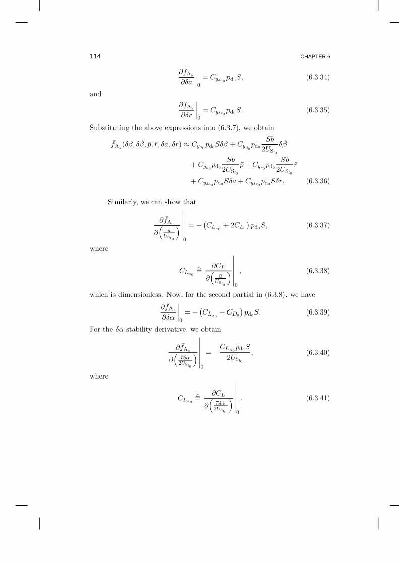
114 CHAPTER 6
∂fAy
∂δa
∣∣∣∣0
= Cyδa0pd0
S, (6.3.34)
and
∂fAy
∂δr
∣∣∣∣0
= Cyδr0pd0
S. (6.3.35)
Substituting the above expressions into (6.3.7), we obtain
fAy(δβ, δβ, p, r, δa, δr) ≈ Cyβ0
pd0Sδβ + Cyβ0
pd0
Sb
2USf0
δβ
+ Cyp0pd0
Sb
2USf0
p+ Cyr0pd0
Sb
2USf0
r
+ Cyδa0pd0
Sδa+ Cyδr0pd0
Sδr. (6.3.36)
Similarly, we can show that
∂fAz
∂(
uUSf0
)
∣∣∣∣∣∣∣0
= −(CLu0
+ 2CL0
)pd0
S, (6.3.37)
where
CLu0
=∂CL
∂(
uUSf0
)
∣∣∣∣∣∣∣0
, (6.3.38)
which is dimensionless. Now, for the second partial in (6.3.8), we have
∂fAz
∂δα
∣∣∣∣0
= −(CLα0
+ CD0
)pd0
S. (6.3.39)
For the δα stability derivative, we obtain
∂fAz
∂(
cδα2USf0
)
∣∣∣∣∣∣∣0
= −CLα0
pd0S
2USf0
, (6.3.40)
where
CLα0
=∂CL
∂(
cδα2USf0
)
∣∣∣∣∣∣∣0
. (6.3.41)

STATIC STABILITY AND STABILITY DERIVATIVES 115
For the pitch-rate stability derivative, we obtain
∂fAz
∂(
cq2USf0
)
∣∣∣∣∣∣∣0
= −CLq0
pd0S
2USf0
. (6.3.42)
Note that CLq0> 0 due to the angle of attack of the tail. Substituting into
(6.3.8), we have
fAz(u, δα, δα, q, δe) ≈
(CLu0
+ 2CL0
)pd0
Su
USf0
+(CLα0
+CD0
)pd0
Sδα + CLα0pd0
Sδα
(c
2USf0
)
+ CLq0pd0
Sq
(c
2USf0
)
+ CLδe0pd0
Sδe. (6.3.43)
6.4 Aerodynamic Moment Coefficients
For moment coefficients, we have Taylor expansions for the roll coeffi-cient
LA
pdSb= Cl(δβ, δβ, δa, δr)
≈ Cl0 +Clβ0δβ +
b
2USf0
Clβ0δβ +Clδa0
δa+ Clδr0δr, (6.4.1)
the pitch coefficient
MA
pdSc= Cm(α0 + δα, u, δe) ≈ Cm0
+ Cmα0δα+
1
USf0
Cmu0u+ Cmδe0
δe,
(6.4.2)
and the yaw coefficient
NA
pdSb= Cn(δβ, δβ, δr, δa)
≈ Cn0+ Cnβ0
δβ +b
2USf0
Cnβ0δβ + Cnδr0
δr + Cnδa0δa. (6.4.3)
Here, Clβ0, Cmα0
, and Cnβ0are stability derivatives, Clδa0
, Cmδr0, and
Cnδr0are control derivatives, and Clδr0
and Cnδa0are cross control deriva-
tives. Note that
Clβ=∂Cl∂β
, (6.4.4)

116 CHAPTER 6
K ΓUΓ
Figure 6.4.2Dihedral wings with angle Γ . The aircraft is pointing out of the page.
Cmα
=∂Cm∂α
, (6.4.5)
and
Cnβ
=∂Cn∂β
. (6.4.6)
6.4.1 Clβ0
Suppose the aircraft velocityV AC is perturbed by ∆
V AC with δβ > 0.
We need LA < 0 and hence Clβ0< 0 in order to roll away from the sideslip
perturbation and thus reduce the sideslip perturbation in accordance withstatic stability. Note that δα increases as δβ decreases.
Clβ0is the stability derivative corresponding to the roll moment LA
caused by sideslip. It is affected by the fuselage, the wing dihedral, the wingposition on the fuselage, and its sweep angle.
6.4.1.1 Effect of Wing Dihedral on Clβ0
We first consider the wing dihedral with the aircraft sideslipping tothe right, as shown in Fig. 6.4.2.
Note that, if Γ > 0, the wing is dihedral, otherwise it is anhedral. InFig. 6.4.3, Vn1
is the normal component of Vair due to V , and Vn2is the
normal component of Vair due to W . The normal velocityV n of
V air on the
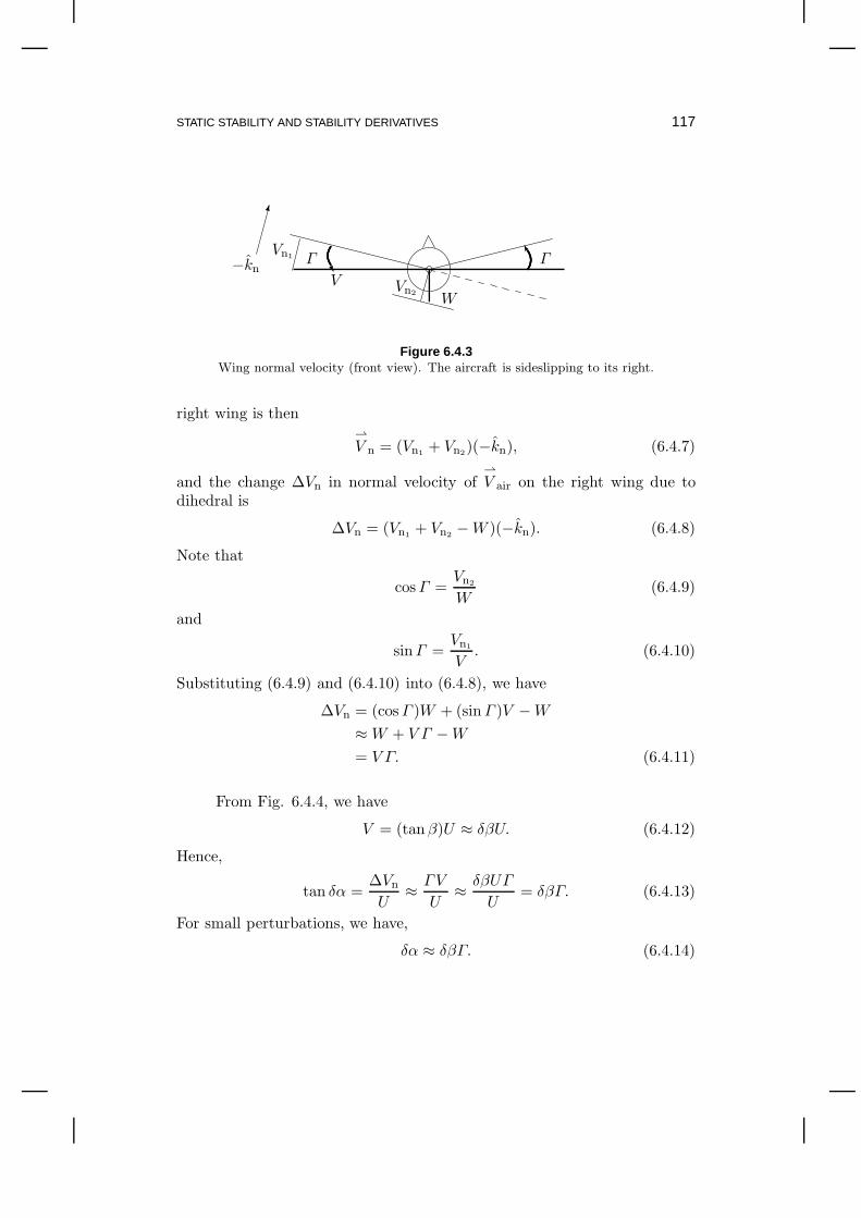
STATIC STABILITY AND STABILITY DERIVATIVES 117
VUΓ
Vn1
−knK Γ
WVn2
Figure 6.4.3Wing normal velocity (front view). The aircraft is sideslipping to its right.
right wing is thenV n = (Vn1
+ Vn2)(−kn), (6.4.7)
and the change ∆Vn in normal velocity ofV air on the right wing due to
dihedral is
∆Vn = (Vn1+ Vn2
−W )(−kn). (6.4.8)
Note that
cosΓ =Vn2
W(6.4.9)
and
sinΓ =Vn1
V. (6.4.10)
Substituting (6.4.9) and (6.4.10) into (6.4.8), we have
∆Vn = (cosΓ )W + (sinΓ )V −W
≈W + V Γ −W
= V Γ. (6.4.11)
From Fig. 6.4.4, we have
V = (tanβ)U ≈ δβU. (6.4.12)
Hence,
tan δα =∆Vn
U≈ ΓV
U≈ δβUΓ
U= δβΓ. (6.4.13)
For small perturbations, we have,
δα ≈ δβΓ. (6.4.14)

118 CHAPTER 6
wing cross section
*V AC,proj + ∆
V n
6
∆V nK δα
: V AC,proj
α0
K
Figure 6.4.4Perturbed angle of attack.
Thus, α0 is perturbed by δα, which effectively increases the angle of attackof the right wing due to sideslipping to the right, as shown in Fig. 6.4.5. Asimilar analysis shows that, on the left wing, the angle of attack is decreasedby δα. This effect results in a negative roll moment. Hence Clβ0
< 0, whichimplies static stability.
6.4.1.2 Effect of Wing Position on Clβ0
Consider first a high wing as in Fig. 6.4.6. The cross flow field velocitydue to sideslip to the right is equal to δβU . This sideslip causes the aircraftto roll to the left, with a roll moment LA < 0. Hence, since positive sideslipinduces a negative roll moment, it follows that Clβ0
< 0. Hence high winghas the same effect as wing dihedral.
Consider now a low wing as in Fig. 6.4.7, and a positive sideslippingto the right, with, again, a flow field velocity δβU . In this case, Clβ0
> 0,and a positive sideslip induces a positive roll moment, while a negativesideslip causes a negative roll moment. Wing dihedral is sometimes used tocounteract this effect.
6.4.1.3 Effect of Wing sweep on Clβ0
As shown in Fig. 6.4.8, the sweep angle of the wings affects the aircraftresponse to sideslip. A sideslip to the right causes increased lift by the rightwing, and thus, causes a negative roll moment.

STATIC STABILITY AND STABILITY DERIVATIVES 119
V
U
V AC
V air
δβ
Figure 6.4.5Effect of sideslip and dihedral.
?
δα < 06
δα > 0
Figure 6.4.6High wing (front view). The aircraft is sideslipping to its right. The flow around the
fuselage perpendicular to the wing produces a negative roll moment.
6
δα > 0
?
δα < 0
Figure 6.4.7Low wing (front view). The aircraft is sideslipping to its right. The flow around the
fuselage perpendicular to the wing produces a positive roll moment.

120 CHAPTER 6
>
>
>
>
>
Vair
Figure 6.4.8Clβ0
is negative due to wing sweep since for δβ > 0 the lift of the right wing is greaterthan the lift of the left wing.
Finally, note that Clβ0is also affected by the horizontal and vertical
tails.
6.4.2 Cmα0
For pitch static stability, we perturb α0 to α0 + δα, and obtain
Cm(α0 + δα) ≈ Cm0+ Cmα0
δα, (6.4.15)
where Cm0
= Cm(α0) and the pitch moment is
MA = MA0+ mA, (6.4.16)
with
MA0= Cm0
pdSc. (6.4.17)
The perturbed moment is
MA = Cm(α0 + δα)pdSc
= Cm0pdSc+ ∆CmpdSc, (6.4.18)
where
∆Cm= Cm(α0 + δα) − Cm(α0)
≈ Cmα0δα. (6.4.19)

STATIC STABILITY AND STABILITY DERIVATIVES 121
?WAC
•c
?kE
O
L
WkS
U kAC
cp •
• ac
xcp
xac
xc
0
ıAC*
K α0:
V AC
: ıS-ıE
9
D
Figure 6.4.9Pitching moment analysis assuming zero sideslip.
Hence, the change in moment is
mA = ∆CmpdSc ≈ Cmα0pdScδα. (6.4.20)
If δα > 0, that is, the nose goes up, then the change in moment is negative.Thus,
∆Cm < 0, (6.4.21)
and hence
Cmα0≈ ∆Cm
δα< 0. (6.4.22)
We link Cmαto the center of mass c. First, referring to Fig. 6.4.9, we
note the following properties:
• ac is the aerodynamic center, which is usually fixed, with xac = c/4.
• The momentMac = MacS (6.4.23)
about ac is independent of α and is generally nonzero.
• cp is the center of pressure, where xcp moves as α changes.

122 CHAPTER 6
• The moment about cp is zero for all α.
We compute the momentM c about the center of mass,
M c = (xc − xcp)
︸ ︷︷ ︸
<0
ıAC ×L
= (xc − xac)ıAC ×L
︸ ︷︷ ︸
aerodynamic moment
+ (xac − xcp)ıAC ×L
︸ ︷︷ ︸
aerodynamic moment
= (xc − xac)L(cosα)S +Mac
= [(xc − xac)L+Mac](cosα)S∼= [(xc − xac)︸ ︷︷ ︸
<0
L+Mac︸︷︷︸
<0
]S. (6.4.24)
WritingM c = McS, (6.4.25)
we have
Mc
pdSc= [(xc − xac)L+Mac]
1
pdSc
or
Mc
pdSc=xc − xac
c
L
pdS+Mac
pdSc. (6.4.26)
Therefore, defining
Cmc
=Mc
pdSc, (6.4.27)
we have
Cmc=xc − xac
cCL + Cmac
, (6.4.28)
where the pitch moment coefficient Cmacis independent of α. Since Cmα
=Cmc
, we have
Cmα=xc − xac
cCLα
+ 0. (6.4.29)
At the nominal flight conditions, (6.4.29) becomes
Cmα0=xc − xac
cCLα0
. (6.4.30)
Since xc − xac < 0 we have Cmα0< 0 with static stability as shown. On
the other hand, if xc − xac > 0, then Cmα0> 0 and the aircraft is statically
unstable.

STATIC STABILITY AND STABILITY DERIVATIVES 123Cm
α
C ′
mα
•α′
0
new trimdue to increasedmass at nose
Cmα
•
original trim
α0
Figure 6.4.10Change in pitching moment coefficient due to a change in trim.
Now suppose that additional mass is added at the nose. Then, fromFig. 6.4.10, we can see that C ′
mα< Cmα
< 0. Hence, Cmαbecomes more
negative as xc decreases.
6.4.3 Cnβ0
Now suppose that yaw is perturbed so that the sideslip angle isnonzero. For the yawing moment we have
NA = CnpdSb,
where Cn is the yawing moment coefficient. Using the Taylor expansion, weexpress
Cn(β0 + δβ, δβ, δa, δr)
≈ Cn0+ Cnβ0
δβ +b
2USf0
Cnβ0δβ + Cnδa0
δa+ Cnδr0δr, (6.4.31)
where Cnβ0is the static directional stability derivative, or weather vane sta-
bility derivative defined by
Cnβ
=∂Cn∂β
, (6.4.32)

124 CHAPTER 6
Cnδa0is the adverse aileron-yaw effect, usually negative, and Cnδr0
is therudder control derivative. For a symmetric airfoil, Cn0
= 0.
Cnβ0> 0 implies static stability since sideslip to the right causes a yaw
moment to the right.
Suppose δβ > 0. In terms of static stability, rolling away from sideslipso that δβ decreases is statically stable. Furthermore, yawing into sideslipso that δβ decreases is statically stable.
Consider a perturbation δα of α0 yielding the angle of attack α0 + δα.Then, |δα| decreases to zero if Cmα0
< 0.
Now let β0 = 0. For a small perturbation δβ, the aircraft rolls awayfrom δβ due to Clβ0
< 0.
Hence, due to Cmα0, the aircraft returns to its original pitch angle, but
Clβ0causes the aircraft to roll and ultimately attain a new heading. Hence,
the aircraft is asymptotically stable in pitch and semistable in heading.
6.5 Linearization of Moments in FSf
We now look at the perturbed aerodynamic moments in the frozenstability frame FSf
. We can express the pitch-moment perturbation mAC asa function of u, δα, δα, q, and δe. Using a Taylor expansion, we write
mA(u, δα, δα, q, δe) ≈ ∂mA
∂u
∣∣∣∣0
u+∂mA
∂δα
∣∣∣∣0
δα +∂mA
∂δα
∣∣∣∣0
δα
+∂mA
∂q
∣∣∣∣0
q +∂mA
∂δe
∣∣∣∣0
δe. (6.5.1)
Likewise, the lateral moments lA and nA can be expressed as functions ofδβ, δβ, p, r, δa, and δr.
In order to nondimensionalize the longitudinal and lateral moment
partial derivatives, we use uUSf0
,(
c2USf0
)
δα,(
b2USf0
)
δβ,(
b2USf0
)
p,(
c2USf0
)
q,
and(
b2USf0
)
r.
At steady state, we can show that
∂mA
∂(
uUSf0
)
∣∣∣∣∣∣∣0
=(Cmu0
+ 2Cm0
)pd0
Sc, (6.5.2)
STATIC STABILITY AND STABILITY DERIVATIVES 125
where
Cmu
=∂Cm
∂(
uUSf0
) . (6.5.3)
Note that Cmu0, which is the Mach tuck derivative, changes with
V AC. Cm0
is the aerodynamic trim moment to counter the thrust moment. Note thatwhen u increases, xac shifts toward the back of the plane. From (6.4.29),Cmα
< 0, which means that the nose goes down. Hence, the pitch momentmust be negative, which results in Cm < 0 at USf0
+ u, and thus Cmu0< 0.
Now, differentiating with respect to δα, we have
∂mA
∂δα
∣∣∣∣0
= Cmα0pd0
Sc, (6.5.4)
where
Cmα0
=∂Cm∂δα
∣∣∣∣0
. (6.5.5)
For the δα derivative, we obtain
∂mA
∂(
cδα2USf0
)
∣∣∣∣∣∣∣0
=Cmα0
pd0Sc
2USf0
, (6.5.6)
where
Cmα0
=∂Cm
∂(
cδα2USf0
)
∣∣∣∣∣∣∣0
. (6.5.7)
For the pitch-rate derivative, we obtain
∂mA
∂(
qc2USf0
)
∣∣∣∣∣∣∣0
=Cmq0
pd0Sc
2USf0
, (6.5.8)
where the pitch damping derivative is defined by
Cmq0
=∂Cm
∂(
cq2USf0
)
∣∣∣∣∣∣∣0
(6.5.9)
and where Cmq0< 0. Finally, for the δe derivative, we obtain
∂mA
∂δe
∣∣∣∣0
= Cmδe0pd0
Sc. (6.5.10)

126 CHAPTER 6
Finally, using (6.5.2), (6.5.4), (6.5.6), (6.5.8), and (6.5.10), (6.5.1) becomes
mA(u, δα, δα, q, δe) ≈(Cmu0
+ 2Cm0
)pd0
Sc
USf0
u+ Cmα0pd0
Scδα
+ Cmα0pd0
Sc2
2USf0
δα +Cmq0pd0
Sc2
2USf0
q
+ Cmδe0pd0
Scδe. (6.5.11)
6.6 Effect of Adverse Control Derivatives
6.6.1 Adverse Aileron-Yaw
As shown in Fig. 6.6.11, since the left wing has increased lift due toaileron down, it also has increased drag. Hence, the aircraft turns right butsideslips to the left, which explains the “adverse” terminology. To cancelthis moment, we can use the rudder δr. From the yaw moment equation(6.4.31), we have
Cnδr0δr + Cnδa0
δa = 0, (6.6.1)
or,
δr =−Cnδa0
Cnδr0
δa. (6.6.2)
Note that Cnδa0and Cnδr0
do not change sign, whereas δa and δrchange sign as these control surfaces move. The adverse aileron-yaw momentis due to Cnδa0
< 0.
6.6.2 Adverse Rudder-Roll
To cancel the adverse rudder-roll moment, we use the aileron as shownin Fig. 6.6.12. From (6.4.1), we write
Clδr0δr + Clδa0
δa = 0. (6.6.3)
Solving for the aileron δa, we obtain
δa =−Clδr0
Clδa0
δr. (6.6.4)
Note that Cnδa0and Cnδr0
do not change sign, whereas δa and δrchange sign as these control surfaces move. However, the sign of Clδr0
de-pends on the angle of attack. To see this, it is helpful to view the rudder as

STATIC STABILITY AND STABILITY DERIVATIVES 127
down
roll r i g h t
less lift, less drag
upδa > 0
yaw left
more lift, more drag
Figure 6.6.11Adverse aileron-yaw.
u α α q δeSurge CD ±Pitch Cm
Plunge CL
Table 6.1 Longitudinal stability derivatives and control.
producing a forcef δr on the vertical tail along the AC axis in the direction
opposite to the rudder deflection. Now, consider the use of left rudder sothat δr > 0 and the yaw moment is negative. For high α, that is, for largepositive α, the roll moment is negative. Hence the roll due to rudder isconsistent with the yaw motion, and thus is proverse. In this case, Clδr0
isnegative. On the other hand, for low α, that is, large negative α, the rollmoment is positive. Hence the roll due to rudder opposes the yaw motion,and thus is adverse. In this case, Clδr0
is positive.
6.7 Problems
Problem 6.7.1 Consider the expression (6.6.2), which shows how toset the rudder to cancel adverse aileron-yaw. Then draw two diagrams (onefor right rudder and one for left rudder) and check the signs of all terms in

128 CHAPTER 6
AC
α
αlowV
AC
high
VAC
i
δr > 0
fδr
Figure 6.6.12Adverse and proverse rudder-roll.
δβ δβ p r δa δeRoll Cl < 0Sway Cy < 0Yaw Cn
Table 6.2 Lateral stability derivatives and control.
the equation to confirm that they are all correct.
Problem 6.7.2 Consider the expression (6.6.4), which shows how toset the ailerons to cancel adverse rudder-roll. Then draw two diagrams (onefor rudder right and one for rudder left) and check the signs of all terms inthe equation to confirm that they are all correct.
Problem 6.7.3 Determine the linearized expression for the frozen sta-bility frame roll-moment perturbation lA.

Chapter Seven
Linearized Equations of Motion
7.1 Longitudinal Equations of Motion
We now incorporate the stability derivatives within the linearizedequations of motion (5.7.20)-(5.7.25). Note that we divide by the mass mand inertia Iyy to solve for linear and angular acceleration. For the linearizedlongitudinal equations, we obtain
˙u =pd0
S
mUSf0
(CD0
CDu0− Cy0Cyu0
Cx0
+ 2√
C2D0
− C2y0
)
︸ ︷︷ ︸
Xu0
u
+pd0
S
mUSf0
(CFTxu0
+ 2CFTx0
)
︸ ︷︷ ︸
XFTu0
u+pd0
S
m
(CD0
CDα0−Cy0Cyα0
Cx0
+CL0
)
︸ ︷︷ ︸
Xα0
δα
+pd0
Sc
2mUSf0
(CD0
CDα0− Cy0Cyα0
Cx0
)
︸ ︷︷ ︸
Xα0
δα +pd0
Sc
2mUSf0
(CD0
CDq0− Cy0Cyq0
Cx0
)
︸ ︷︷ ︸
Xq0
q
− g(cos γ0)θ +pd0
S
m
(CD0
CDδe0− Cy0Cyδe0
Cx0
)
︸ ︷︷ ︸
Xδe0
δe, (7.1.1)

130 CHAPTER 7
˙w =pd0
S
mUSf0
(CLu0+ 2CL0
)
︸ ︷︷ ︸
Zu0
u+pd0
S
mUSf0
(CFTzu0
+ 2CFTz0
)
︸ ︷︷ ︸
ZFTw0
u
+pd0
S
m(CLα0
+ CD0)
︸ ︷︷ ︸
Zα0
δα +pd0
Sc
2mUSf0
CLα0
︸ ︷︷ ︸
Zα0
δα
+ USf0q +
pd0Sc
2mUSf0
CLq0
︸ ︷︷ ︸
Zq0
q − g(sin γ0)θ +pd0
S
mCLδe0
︸ ︷︷ ︸
Zδe0
δe, (7.1.2)
and
˙q =pd0
Sc
IyyUSf0
(Cmu0+ 2Cm0
)
︸ ︷︷ ︸
Mu0
u+pd0
Sc
IyyUSf0
(CmFTu0
+ 2CmFT0
)
︸ ︷︷ ︸
MFTu0
u
+pd0
Sc
IyyCmα0
︸ ︷︷ ︸
Mα0
δα +pd0
Sc
IyyCmFTα0
︸ ︷︷ ︸
MFTα0
δα+pd0
Sc2
2IyyUSf0
Cmα0
︸ ︷︷ ︸
Mα0
δα
+pd0
Sc2
2IyyUSf0
Cmq0
︸ ︷︷ ︸
Mq0
q +pd0
Sc
IyyCmδe0
︸ ︷︷ ︸
Mδe0
δe. (7.1.3)
Hence, we have the linearized surge, plunge, and pitch-rate equations
˙u =(
Xu0+XFTu0
)
u+Xα0δα +Xα0
δα+Xq0 q − g(cos γ0)θ +Xδe0δe,
(7.1.4)
˙w = (Zu0+ ZFTw0
)u+ Zα0δα+ Zα0
δα +(USf0
+ Zq0)q
− g(sin γ0)θ + Zδe0δe, (7.1.5)
and
˙q =(
Mu0+MFTu0
)
u+(
Mα0+MFTα0
)
δα+Mα0δα +Mq0 q +Mδe0δe.
(7.1.6)
Note that
w ≈ USf0δα
and
˙w ≈ USf0δα.

LINEARIZED EQUATIONS OF MOTION 131
Hence, in terms of δα, (7.1.5) can be written as
δα =Zu0
+ ZFTw0
USf0
u+Zα0
USf0
δα +Zα0
USf0
δα+
(USf0
+ Zq0USf0
)
q
− g(sin γ0)
USf0
θ +Zδe0USf0
δe. (7.1.7)
7.2 Linearized Longitudinal Equations and TransferFunctions
We can write the linearized longitudinal equations (7.1.4), (7.1.6), and(7.1.7) in state space form as
˙uδα˙q
θ
=
Xu0+XFTu0
Xα00 −g cos γ0
Zu0+ZFTw0
USf0−Zα0
Zα0
USf0−Zα0
USf0+Zq0
USf0−Zα0
−g sinγ0USf0
−Zα0
Mu0+MFTu0
Mα0+MFTα0
Mq0 0
0 0 1 0
uδαqθ
+
Xδe0
Zδe0
USf0−Zα0
Mδe0
0
δe. (7.2.1)
Taking the Laplace transform of the longitudinal equations, we obtain
sˆu = (Xu0+XFTu0
)ˆu+Xα0δ ˆα− g(cos γ0)θ +Xδe0δe, (7.2.2)
s(USf0− Zα0
)δα = (Zu0+ ZFTw0
)ˆu+ Zα0δα+ [(USf0
+ Zq0)s− g sin γ0]θ
+ Zδe0δe, (7.2.3)
and
s2θ = (Mu0+MFTu0
)ˆu+ (Mα0+MFTα0
)δα +Mq0sθ +Mδe0δe. (7.2.4)

132 CHAPTER 7
Stability
ParameterDefinition Units
Xu0
pd0S
mUSf0
(CD0
CDu0−Cy0
Cyu0
Cx0
+ 2√
C2D0
− C2y0
)
1/sec
XFTu0
pd0S
mUSf0
(CFTxu0
+ 2CFTx0
) 1/sec
Xα0
pd0S
m
(CD0
CDα0−Cy0
Cyα0
Cx0
+ CL0
)
ft/sec2-rad
Xα0
pd0Sc
mUSf0
(CD0
CDα0−Cy0
Cyα0
Cx0
)
ft − sec/rad
Xq0pd0
ScmUSf0
(CD0
CDq0−Cy0
Cyq0
Cx0
)
1/sec
Xδe0pd0
Sm
(CD0
CDδe0−Cy0
Cyδe0
Cx0
)
ft/sec2-rad
Zu0
pd0S
mUSf0
(CLu0+ 2CL0
) 1/sec
Zα0
pd0S
m (CLα0+ 2CD0
) ft/sec2-rad
Zα0
pd0Sc
2mUSf0
CLα0ft/sec-rad
Zq0pd0
Sc2mUSf0
CLq0ft/sec-rad
Zδe0pd0
Sm CLδe0
ft/sec2-rad
ZFTw0
pd0S
mUSf0
(CFTzu0
+ 2CFTz0
) 1/sec
Mu0
pd0Sc
IyyUSf0
(Cmu0+ 2Cm0
) rad/ft-sec
MFTu0
pd0Sc
IyyUSf0
(CmFTu0
+ 2CmFT0
) 1/ft-sec
Mα0
pd0Sc
IyyCmα0
1/sec2
MFTα0
pd0Sc
IyyCmFTα0
1/sec2
Mα0
pd0Sc2
2IyyUSf0
Cmα01/sec
Mq0pd0
Sc2
2IyyUSf0
Cmq01/sec
Mδe0pd0
Sc
IyyCmδe0
1/sec2
Table 7.1 Longitudinal stability parameters.

LINEARIZED EQUATIONS OF MOTION 133
Thus,
s −
(
Xu0+ XFTu0
)
−Xα0g cos γ0
−(Zu0+ ZFTw0
)(
USf0− Zα0
)
s − Zα0−
(
USf0+ Zq0
)
s + g sin γ0
−
(
Mu0+ MFTu0
)
−
(
Mα0+ MFTα0
)
s2− Mq0s
[ˆu
δα
θ
]
=
Xδe0
(USf0− Zα0
)Zδe0Mδe0
δe. (7.2.5)
Inverting the 3 × 3 matrix coefficient in (7.2.5) yields
Gu/δe(s) =ˆu(s)
δe(s)=
Aus3 +Bus
2 + Cus+Du
s4 + Es3 + Fs2 +Gs+H, (7.2.6)
Gδα/δe(s) =δα(s)
δe(s)=Aαs
3 +Bαs2 + Cαs+Dα
s4 + Es3 + Fs2 +Gs+H, (7.2.7)
and
Gθ/δe(s) =θ(s)
δe(s)=
Bθs2 + Cθs+Dθ
s4 + Es3 + Fs2 +Gs+H. (7.2.8)
Note that the numerator in (7.2.8) is second order, see Problem 7.5.1.
The denominator p(s) = s4 +Es3 + Fs2 +Gs+H can be factored as
p(s) = (s2 + 2ζspωn,sps+ ω2n,sp)(s
2 + 2ζphωn,phs+ ω2n,ph). (7.2.9)
Although p(s) cannot be factored symbolically, it can always be factorednumerically. It has four roots given by two complex conjugate pairs thatdepend on the flight condition, the mass distribution, and the airplane ge-ometry.
7.3 Lateral Equations of Motion
Similarly, we obtain the lateral equations of motion
˙v =pd0
S
mCyβ0
︸ ︷︷ ︸
Yβ0
δβ +pd0
Sb
2mUSf0
Cyβ0
︸ ︷︷ ︸
Yβ0
δβ +pd0
Sb
2mUSf0
Cyp0
︸ ︷︷ ︸
Yp0
p
+pd0
Sb
2mUSf0
Cyr0
︸ ︷︷ ︸
Yr0
r − USf0r + g(cos Θ0)φ+
pd0S
mCyδa0
︸ ︷︷ ︸
Yδa0
δa+pd0
S
mCyδr0
︸ ︷︷ ︸
Yδr0
δr,
(7.3.1)

134 CHAPTER 7
˙p =IxzIzz
˙r +
pd0Sb
IxxClβ0
︸ ︷︷ ︸
Lβ0
+pd0
S
IzzClFTβ0
︸ ︷︷ ︸
LFTβ0
δβ +pd0
Sb2
2IxxUSf0
Clp0
︸ ︷︷ ︸
Lp0
p
+pd0
Sb2
2IxxUSf0
Clr0
︸ ︷︷ ︸
Lr0
r +pd0
Sb
IxxClδa0
︸ ︷︷ ︸
Lδa0
δa +pd0
Sb
IxxClδr0
︸ ︷︷ ︸
Lδr0
δr, (7.3.2)
and
˙r =IxzIzz
˙p+
pd0Sb
IzzCnβ0
︸ ︷︷ ︸
Nβ0
+pd0
Sb
IzzCnFTβ0
︸ ︷︷ ︸
NFTβ0
δβ +pd0
Sb2
2IzzUSf0
Cnp0
︸ ︷︷ ︸
Np0
p
+pd0
Sb2
2IzzUSf0
Cnr0
︸ ︷︷ ︸
Nr0
r +pd0
Sb
IzzCnδa0
︸ ︷︷ ︸
Nδa0
δa+pd0
Sb
IzzCnδr0
︸ ︷︷ ︸
Nδr0
δr. (7.3.3)
Using stability parameter notation, we can write (7.3.1)-(7.3.3) as
˙v = Yβ0δβ + Yβ0
δβ + Yp0p− USf0r + Yr0 r + g(cos Θ0)φ+ Yδa0
δa+ Yδr0δr,
(7.3.4)
˙p =IxzIzz
˙r + (Lβ0+ LFTβ0
)δβ + +Lp0 p+ Lr0 r + Lδa0δa+ Lδr0δr, (7.3.5)
and
˙r =IxzIzz
˙p+Nβ0δβ +NFTβ0
δβ +Np0 p+Nr0 r +Nδa0δa+Nδr0δr. (7.3.6)
Using
δβ ≈ v
USf0
, (7.3.7)
thus,
v ≈ δβUSf0(7.3.8)
and
v ≈ δβUSf0. (7.3.9)

LINEARIZED EQUATIONS OF MOTION 135
Then we can rewrite (7.3.4) as
δβ =Yβ0
USf0
δβ +Yβ0
USf0
δβ +Yp0USf0
p− r +Yr0USf0
r +g(cos Θ0)
USf0
φ
+Yδa0
USf0
δa+Yδr0USf0
δr. (7.3.10)
7.4 Linearized Lateral Equations and TransferFunctions
The lateral linearized equations were given by (7.3.4), (7.3.5), and(7.3.6). The linearized perturbation states are the sideslip, roll rate, yawrate, roll angle, yaw angle and sway. There are two control inputs, δa andδr. For the linearized lateral equations, we obtain
δβ˙p˙r˙φ
= R
Yβ0
USf0−Yβ0
Yp0
USf0−Yβ0
Yr0−USf0
USf0−Yβ0
g cos Θ0
USf0−Yβ0
Lβ0+ LFTβ0
Lp0 Lr0 0
Nβ0+NFTβ0
Np0 Nr0 0
0 0 1 0
δβprφ
+R
Yδa0Yδr0
Lδa0Lδr0
Nδa0Nδr0
0 0
[δaδr
]
. (7.4.1)
where
R
=
1 0 0 0
0 1 − Ixz
Izz0
0 − Ixz
Izz1 0
0 0 0 1
−1
=
1 0 0 0
0 I2zz
I2zz−I2xz
Ixz Izz
I2zz−I2xz
0
0 Ixz Izz
I2zz−I2xz
I2zz
I2zz−I2xz
0
0 0 0 1
. (7.4.2)
We now use the small angle approximation for the derivatives of the

136 CHAPTER 7
Stability parameter Definition Units
Yβ0
pd0S
m Cyβ0ft/sec2-rad
Yβ0
pd0Sb
2mUSf0
Cyβ0ft/sec-rad
Yp0pd0
Sb2mUSf0
Cyp0ft/sec-rad
Yr0pd0
Sb2mUSf0
Cyr0ft/sec-rad
Yδa0
pd0S
m CDδa0ft/sec2-rad
Yδr0pd0
Sm CDδr0
ft/sec2-rad
Lβ0
pd0Sb
IxxClβ0
1/sec2
Lp0pd0
Sb2
2IxxUSf0
Clp01/sec
Lr0pd0
Sb2
2IzzUSf0
Cnp01/sec
Lδa0
pd0Sb
IxxClδa0
1/sec2
Lδr0pd0
Sb
IxxClδr0
1/sec2
LFTβ0
pd0S
IzzClFTβ0
1/sec2
Nβ0
pd0Sb
IzzCnβ0
1/sec2
NFTβ0
pd0Sb
IzzCnFTβ0
1/sec2
Np0pd0
Sb2
2IzzUSf0
Cnp01/sec
Nr0pd0
Sb2
2IzzUSf0
Cnr01/sec
Nδa0
pd0Sb
IzzCnδa0
1/sec2
Nδr0pd0
Sb
IzzCnδr0
1/sec2
Table 7.2 Lateral stability parameters.

LINEARIZED EQUATIONS OF MOTION 137
3-2-1 Euler-angle perturbations given by (5.7.5) to obtain
ψ
θ
φ
=
sin γ0 0 cosα0
0 1 0cos γ0 0 − sinα0
−1
pqr
=1
cos Θ0
sinα0 0 cosα0
0 cos Θ0 0cos γ0 0 − sin γ0
pqr
=
(sinα0)p+(cosα0)rcos Θ0
q
(cos γ0)p−(sin γ0)rcos Θ0
. (7.4.3)
Hence, the derivatives of the Euler-angle perturbations are given in termsof the angular velocity vector perturbations in the frozen stability frame by
ψ =(sinα0)p+ (cosα0)r
cos Θ0, (7.4.4)
θ = q, (7.4.5)
φ =(cos γ0)p− (sin γ0)r
cos Θ0. (7.4.6)
Taking Laplace transforms of the linearized lateral equations yields
(USf0− Yβ0
)sδβ = Yβ0δβ + Yp0s
ˆφ+ (Yr0 − USf0)s ˆψ + g(cos Θ0)
ˆφ
− (USf0− Yβ0
)Yδa0δa+ (USf0
− Yβ0)Yδr0δr, (7.4.7)
s2 ˆφ =IxzIzz
s2 ˆψ + (Lβ0+ LFTβ0
)δβ + Lp0sˆφ+ Lr0s
ˆψ + Lδa0δa+ Lδr0δr,
(7.4.8)
s2 ˆψ =IxzIzz
s2 ˆφ+ (Nβ0+NFTβ0
)δβ +Np0sˆφ+Nr0s
ˆψ +Nδa0δa+Nδr0δr.
(7.4.9)
Then, using these approximations and taking the Laplace transform,

138 CHAPTER 7
the linearized equations become
s(USf0− Yβ0
) − Yβ0−(sYp0 + g cos Θ0) s(USf0
− Yr0)
−Lβ0− LFTβ0
s2 − sLp0 −(s2 Ixz
Ixx+ sLr0)
−Nβ0−NFTβ0
−(s2 Ixz
Izz+ sNp0) s2 − sNr0
β(s)
φ(s)
ψ(s)
=
(USf0− Yβ0
)Yδa0(USf0
− Yβ0)Yδr0
Lδa0Lδr0
Nδa0Nδr0
[δa(s)δr(s)
]
. (7.4.10)
Inverting (7.4.10) yields
Gβ/δa(s) =β(s)
δa(s)=Aβ,δas
3 +Bβ,δas2 + Cβ,δas+Dβ,δa
s4 + E′s3 + F ′s2 +G′s+H ′, (7.4.11)
Gφ/δa(s) =φ(s)
δa(s)=
Bφ,δas2 + Cφ,δas+Dφ,δa
s4 + E′s3 + F ′s2 +G′s+H ′, (7.4.12)
and
Gψ/δa(s) =ψ(s)
δa(s)=
Bψ,δas2 + Cψ,δas+Dψ,δa
s4 + E′s3 + F ′s2 +G′s+H ′. (7.4.13)
For the rudder perturbation, (7.4.10) yields
Gβ/δr(s) =β(s)
δr(s)=Aβ,δrs
3 +Bβ,δrs2 + Cβ,δrs+Dβ,δr
s4 + E′s3 + F ′s2 +G′s+H ′, (7.4.14)
Gφ/δr(s) =φ(s)
δr(s)=
Bφ,δrs2 + Cφ,δrs+Dφ,δr
s4 +E′s3 + F ′s2 +G′s+H ′, (7.4.15)
and
Gψ/δr(s) =ψ(s)
δr(s)=Aψ,δrs
3 +Bψ,δrs2 + Cψ,δrs+Dψ,δr
s(s4 + E′s3 + F ′s2 +G′s+H ′). (7.4.16)
The characteristic equation is written as
p(s) = (s2 + 2ζDrωn,Dr + ω2n,Dr)
(
s+1
τr
)(
s+1
τs
)
= 0. (7.4.17)
From solving (7.4.17), we find the Dutch roll mode, which involves sideslip,roll, yaw oscillations, the roll mode, and the spiral mode. Note that thespiral mode is a slow roll and a slow yaw, and it is stable for Clβ0
<< 0.The roll mode is unstable for large α and τr and has little response to δa.

LINEARIZED EQUATIONS OF MOTION 139
7.4.1 Yaw Stability
Consider the heading perturbation ψ. Since the transfer function(7.4.16) has a pole at 0, it is not asymptotically stable, but rather is semistable.The integrator component of (7.4.16) due to the pole at 0 shows that an im-pulsive change in δr produces a steady-state effect on the heading. Thistype of stability is consistent with the fact that the aircraft has no naturalmechanism to return its heading to the original value after a sideslip or rollperturbation, thus leading to a new steady-state heading angle.
7.5 Problems
Problem 7.5.1 Show that the numerator of the transfer function in(7.2.8) from δe to θ is second order. Hint: Show CB = 0 and Section A.14.
Problem 7.5.2 Determine Au, Aα, and Bθ in terms of the stabilityparameters. Hint: See Section A.14.
Problem 7.5.3 Use (7.4.16) to determine the steady-state heading-angle perturbation from an impulse rudder deflection.


Chapter Eight
Analysis of Flight Modes
8.1 Eigenflight
Eigenflight is the motion of an aircraft near nominal flight as given byan eigensolution of the linearized dynamics. For details see Section A.3.
Consider the linear time invariant system
x(t) = Ax(t) (8.1.1)
with initial condition
x(0) = x0.
Let the solution be of the form
x(t) = Re eλtv, (8.1.2)
which satisfies (8.1.1) with the initial condition
x(0) = Re v = x0. (8.1.3)
Substituting (8.1.2) into (8.1.1) we obtain the eigenvalue-eigenvector equa-tion
Av = λv. (8.1.4)
Note that λ may be complex, in which case the associated eigenvector v mayalso be complex. Now write
λ = −ζωn ± ωn
√
1 − ζ2 = σ + ωd (8.1.5)
and
v = vR + vI, (8.1.6)
and substitute λ and v into (8.1.2). We obtain
x(t) = Re e(σ+ωd)t(vR + vI)
= Re eσt[cos(ωdt) + sin(ωdt)](vR + vI)
= eσt[vR cos(ωdt) − vI sin(ωdt)]. (8.1.7)

142 CHAPTER 8
Alternatively, we can represent each component of v in polar form
v =
r1eφ1
r2eφ2
r3eφ3
r4eφ4
. (8.1.8)
The component-wise magnitude and angle of v are given by
|v| =
r1r2r3r4
, ∡v =
φ1
φ2
φ3
φ4
. (8.1.9)
Substituting v into (8.1.2) yields
x(t) = Re e(σ+ωd)t
r1eφ1
r2eφ2
r3eφ3
r4eφ4
= Re
r1eσte(ωdt+φ1)
r2eσte(ωdt+φ2)
r3eσte(ωdt+φ3)
r4eσte(ωdt+φ4)
, (8.1.10)
where ri cosφi is the initial value of the ith component, eσt is the decayenvelope, and φi is the phase shift of the ith component.
8.2 Phugoid Mode
Solving for the complex roots λph and its conjugate λph in (7.2.9),the root with the lower frequency ωn,ph is the phugoid mode. The phugoidmode is associated with low damping, that is, ζph << 1, and a long periodTph = 2π
ωn,phof oscillation, typically 30 to 120 seconds.
We now show that the phugoid mode is a roller coaster oscillation,which trades kinetic and potential energy. In (7.2.6) and (7.2.8), θ and uare oscillatory and δα ≈ 0, which implies that α is approximately constant.
Consider a 747-100 aircraft flying at 40,000 ft at Mach 0.8. The aircraftstate is x = Ax, where
x =
uδαqθ
,

ANALYSIS OF FLIGHT MODES 143
0.5 1−0.5−1
0.5
1
−0.5
−1
phugoid
shortperiod
Figure 8.2.1Phugoid and short period eigenvalues.
and
A =
−2.02e(−2) 7.88 −6.5e(−1) −3.22e(+1)−2.54e(−4) −1.02 9.05e(−1) 07.95e(−11) −2.5 −1.39 0
0 0 1 0
.
Solving for the eigenvalues of A we can express
λsp, λsp = −ζspωn,sp ± ωn,sp
√
1 − ζ2sp
and
λph, λph = −ζphωn,ph ± ωn,ph
√
1 − ζ2ph.
We find λph = −0.0087 ± 0.074 for the mode phugoid and λsp = −1.204 ±1.49 for the short period, which are represented in Fig. 8.2.1. Therefore,ωd,ph = 0.074 rad/sec, ωn,ph = 0.0745 rad/sec, ζph = 0.117, ωd,sp = 1.49rad/sec, ωn,sp = 1.92 rad/sec, and ζsp = 0.628. These results are summa-rized in Table 8.1
By scaling the pitch perturbation, the phugoid eigenvector is given by
vph =
−1 m/sec−9.6e(−5) ± 5.0e(−7) rad
1.7e(−4) ± 8.4e(−6) rad/sec−3.8e(−4) ± 2.3e(−3) rad
. (8.2.1)

144 CHAPTER 8
Mode T T1/2 ωn ζ %
phugoid 84.34 sec 79.67 sec 0.0745 rad/sec 0.117 5%
short period 3.27 sec 0.57 sec 1.92 rad/sec 0.628 38%
Table 8.1 Eigenflight mode characteristics.
The component-wise magnitude of vph is
|vph| =
1 m/sec9.6e(−5) rad
1.7e(−4) rad/sec2.33e(−3) rad
(8.2.2)
with phase
∠vph =
0
0.30
2.83
80.62
. (8.2.3)
Using (8.1.10) the eigensolution is written as
x(t) = eσtRe eωd,pht
r1eφ1
r2eφ2
r3eφ3
r4eφ4
= eσt
r1 cos(ωd,pht+ φ1)r2 cos(ωd,pht+ φ2)r3 cos(ωd,pht+ φ3)r4 cos(ωd,pht+ φ4)
. (8.2.4)
It follows from (8.2.2) and (8.2.3) that
θ(t) = 2.33e(−3) cos(ωd,pht+ 1.407)eσt rad. (8.2.5)
Then, we have
u(t) = USf0cos(ωd,pht+ 0)e0.0087t m/sec, (8.2.6)
δα(t) = 9.6e(−5) cos(ωdpht+ 0.005)e0.0087t rad ≈ constant, (8.2.7)
and
θ(t) = 2.33e(−3)ωd,ph sin(ωd,pht+ 1.407)e0.0087t rad/sec. (8.2.8)

ANALYSIS OF FLIGHT MODES 145
The pitch angle is
Θ = α+ γ (8.2.9)
with nominal values
Θ0 = α0 + γ0. (8.2.10)
Then,
θ = δα + δγ, (8.2.11)
where 8.2.7 shows that δα is small compared to θ. Note that α is relativelyconstant although α0 can be very different from zero.
8.3 Short Period Mode
The short period mode is associated with the higher frequency eigen-values in (7.2.9), λsp, and its conjugate λsp. The short period mode isunderdamped with high ζsp but always less than 1, high frequency ωn,sp,and short period period Tsp = 2π
ωn,sp, with Tsp typically about 2 sec.
Solving for λsp and λsp, we obtain
λsp, λsp = −ζspωn,sp ± ωn,sp
√
1 − ζ2sp. (8.3.1)
From numerics, the eigensolution characteristics are that u is constant whileθ and δα oscillate.
8.4 Phugoid Approximation
To approximate the phugoid mode, set δα = 0, γ0 = 0, Zα0= 0,
Zα0= 0, and ZFTw0
= 0. Then (7.2.5) becomes
[
s−(
Xu0+XFTu0
)
−g−Zu0
USf0s
][ˆuδα
]
=
[0
USf0Zδe0
]
δe. (8.4.1)
The characteristic equation then becomes
p(s) = s2 −(
Xu0+XFTu0
)
s− Zu0g
USf0
= 0 (8.4.2)

146 CHAPTER 8
and hence,
ωn,ph ≈√
−Zu0g
USf0
=
[( −gUSf0
) −pd0S(CLu0
+ 2CL0)
mUSf0
]1/2
≈√
gpd0S(CLu0
+ 2CL0)
mU2Sf0
. (8.4.3)
Since CLu0<< CL0
and CL0= mg
pd0S , we obtain
ωn,ph ≈√
gpd0S
mU2Sf0
(2mg
pd0S
)
≈√
2g2
U2Sf0
≈√
2g
USf0
. (8.4.4)
8.4.1 Phugoid Damping
For the phugoid damping we write
ζph ≈−Xu0
+XFTu0
2ωn,ph. (8.4.5)
Table 7.1 implies
Xu0=
−(CDu0+ 2CD0
)pd0S
mUSf0
(8.4.6)
and
XFTu0
=(CFTxu0
+ 2CFTx0
)pd0S
mUSf0
. (8.4.7)
Let set CFTxu0
= 0 and CFTx0
= 0. Then,
ζph =(CDu0
+ 2CD0)pd0
S
2mUSf0ωn,ph
=(CDu0
+ 2CD0)pd0
S
2√
2mg
=(CDu0
+ 2CD0)
2√
2
1
CL0
. (8.4.8)
At low speed, CDu0= 0, and (8.4.8) becomes
CD0√2CL0
, (8.4.9)
which is proportional to 1L/D . At high L/D, ζph is low.

ANALYSIS OF FLIGHT MODES 147
8.5 Short Period Approximation
To approximate the short period mode, set u = 0 in (7.2.5), whichyields
[ (USf0
− Zα0
)s− Zα0
−(USf0
+ Zq0)s+ g sin γ0
−(
Mα0+MFTα0
)
s2 −Mq0s
][δα
θ
]
=
[Zδe0Mδe0
]
δe. (8.5.1)
We now assume that γ0 = 0, Zα0= 0, Zq0 = 0, and MFTα0
= 0. Then,
(8.5.1) becomes[USf0
s− Zα0−USf0
s−Mα0
s2 −Mq0s
] [δα
θ
]
=
[Zδe0Mδe0
]
δe. (8.5.2)
Then, the characteristic equation is obtained from
(s2 −Mq0s)(USf0
s− Zα0
)− USf0
sMα0= 0, (8.5.3)
or,
USf0s3 +
(−Mq0USf0
− Zα0
)s2 +
(Mq0Zα0
−Mα0USf0
)s = 0. (8.5.4)
Dividing by s and USf0, we obtain the quadratic equation
p(s) = s2 −(
Mq0 +Zα0
USf0
)
s+
(Mq0Zα0
USf0
−Mα0
)
= 0. (8.5.5)
Hence, the transfer functions (7.2.7) and (7.2.8) can be written as
δα(s)
δe(s)=Zδe0s+Mδe0USf0
−Mq0Zδe0USf0
p(s)(8.5.6)
and
θ(s)
δe(s)=USf0
Mδe0s+Mα0Zδe0 − Zα0
Mδe0
USf0sp(s)
. (8.5.7)
From (8.5.5), we express
ωn,sp ≈√
Mq0Zα0
USf0
−Mα0(8.5.8)
and
ζsp = −Mq0 +
Zα0
USf0
2ωn,sp. (8.5.9)

148 CHAPTER 8
Note that we need Mα0< 0 for static stability. For dynamic stability we
need
Mα0<Mq0Zα0
USf0
(8.5.10)
and
Mq0 +Zα0
USf0
< 0. (8.5.11)
Now, if the cg of the aircraft is forward enough, ωn,sp becomes
ωn,sp ≈√
−Mα0≈√
−Cmα0pd0
Sc
Iyy. (8.5.12)
Note that ωn,sp increases with −Cmα0and pd0
, and decreases with Iyy. Wealso note that the main component of ζsp isMq0 which is the damping deriva-
tive,Zα0
Mα0
is determined by other aspects and Mα0is due to the horizontal
tail size with Mα0≈ 1
3Mq0 .
8.6 Problems
Problem 8.6.1 The longitudinal dynamics of a business jet have thecharacteristic polynomial
p(s) = s4 + 2.01s3 + 8.05s2 + 0.085s + 0.068.
Check stability using Routh, identify the short period and phugoid roots,determine the damping ratio and natural frequencies of the roots, and com-pute the time for each response to decay by 50%.
Problem 8.6.2 The longitudinal dynamics of an F-104 fighter flyingstraight and level are modeled by the 4th-order system x = Ax, where
x =[
u δα θ θ]T
and the dynamics matrix is given by
A =
−2.02e(−2) 7.88 −3.22e(+1) −6.5e(−1)−2.54e(−4) −1.02 0 9.05e(−1)
0 0 0 17.95e(−11) −2.5 0 −1.39
.
Here, “e” is the matlab notation for powers of 10. Note the order of states,which is slightly different from the order used in class. Then do the following:
i) Compute the phugoid and short period eigenvalues. Plot thesepoles as four ×’s in the s-plane.

ANALYSIS OF FLIGHT MODES 149
ii) Compute the damping ratio, undamped natural frequency, dampednatural frequency, undamped period, and time to 50% decay foreach mode.
Problem 8.6.3 For the F-104:
i) Compute the eigenvector for the phugoid mode, and normalize theθ component to 1.
ii) Convert the phugoid eigenvector into its magnitude and angle com-ponents.
Problem 8.6.4 Simulate the phugoid eigenflight mode of the F-104using the eigensolution x(t) = Re eAtvph, where vph is the phugoid eigenvec-tor. Assume that the initial condition for θ is given by θ(0) = 7.9 degrees.Then use Matlab to plot all four states for 3 full “periods” of the dampedmotion.

Chapter Nine
Control Concepts
9.1 Problems
Problem 9.1.1 Consider the asymptotically stable loop transfer func-tion
L(s) =−1
s2 + 2s+ 3.
Show that the closed-loop transfer function S(s) = 1/(1 + L(s)) is asymp-totically stable, and use Matlab to plot the magnitude and phase Bode plotsfor S. Then, write a Matlab program to show numerically that
∫∞
0ln |S(ω)| dω = 0.
Explain this result in terms of the “balance” between attenuation and am-plification.
Problem 9.1.2 Consider the unstable loop transfer function
L(s) =4
(s− 1)(s + 2).
Show that the closed-loop transfer function S(s) is asymptotically stable,and use Matlab to plot the Bode plots for S. Then, write a Matlab programto show numerically that
∫∞
0ln |S(ω)| dω = π.
Discuss the “balance” between attenuation and amplification.
Problem 9.1.3 Consider the second-order transfer function
G(s) =1
s2 + 3s− 2
controlled by the PI controller
K(s) = KP +KI
s

152 CHAPTER 9
in a servo loop. Determine the values of KP and KI that render the closed-loop system stable by sketching the region in the KP ,KI plane of stabilizinggains.
Problem 9.1.4 Consider the type II control system with plant
G(s) =1
s(s+ 1)
and PI controller
K(s) = KP +KI
s
in a servo loop. Choose values of KP and KI to obtain zero steady stateerror for a ramp command. Use Simulink to simulate the system and chooseKP and KI for good rise time and reasonable overshoot for a step command.Plot the error response for a ramp command, and verify numerically andanalytically that the ramp command error converges to zero.
Problem 9.1.5 Sketch the root loci for the following loop transferfunctions by using the root locus rules given in class and then check yoursketches using Matlab’s root locus function:
i) L(s) = (s+1)(s+2)(s−1)(s−2)(s−3) .
ii) L(s) = (s+2)2
(s+1)(s2+1) .
Problem 9.1.6 Consider the loop transfer function
L(s) =2.5(s + 100)
(s+ 1)2.
Sketch the gain and phase Bode plots of L(s). Use your plot to indicate themagnitude crossover frequency ωmco, the phase crossover frequency ωpco, thegain margin, and the phase margin.
Problem 9.1.7 Consider the damped rigid body plant
G(s) =1
s(s+ 1).
i) Assume unity feedback so that L(s) = G(s). Sketch the Nyquistplot and determine the gain and phase margins.
ii) Instead of unity feedback, consider the lead controller Gc(s) =k(s + 2)/(s + 20) so that L(s) = Gc(s)G(s). For k = 1, use Mat-lab to determine whether the lead provided by this lead controllerincreases the phase margin.

CONTROL CONCEPTS 153
iii) Draw the root locus in terms of k.
iv) Choose k so that the complex conjugate poles have damping ratioζ =
√2/2.
v) For the value of k that you chose, determine the steady state errorfor the unit ramp input 1/s2.
(Hint: You can solve the problem directly by equating the product of (s −a)(s2 + 2ζωns + ω2
n) with the cubic obtained from the closed loop transferfunction with k as the unknown parameter. Then you can get a cubicequation in a or ωn.)


Chapter Ten
Control of Aircraft
10.1 Problems
Problem 10.1.1 At Mach .6, an experimental aircraft has slightlyunstable short period eigenvalues 0.04±0.12 and stable phugoid eigenvalues−4.3 ± 5.7. Wind tunnel testing reveals that the elevator-to-pitch transferfunction has one zero located at −0.2. For proportional control, sketch theroot locus, determine the center and asymptotes, and discuss the stabilityof the closed-loop longitudinal dynamics for high values of k.
Problem 10.1.2 An experimental aircraft has unstable phugoid eigen-values 0.04 ± 0.12 and stable short period eigenvalues −4.3 ± 5.7. Windtunnel testing reveals that, at Mach .6, the elevator-to-pitch transfer func-tion has three real zeros located at −0.3,−1.7,−8.4. Sketch the root locusand discuss the stability of the closed-loop longitudinal dynamics using aconstant feedback controller. Indicate the point on the root locus at whichall poles have at least
√2/2 damping and explain why this minimum value
of damping is desirable.
Problem 10.1.3 The lateral dynamics of an experimental aircraft aremodeled by the transfer function 1/(τs+1), where τ > 0 is a time constant.For this transfer function a basic servo loop is closed with the integral con-troller KI = s.
i) Determine the values of KI for which the closed-loop system isasymptotically stable.
ii) For which values of KI is the steady-state error to a unit-sloperamp command less than 0.025?
iii) For a value of KI such that the closed-loop system is asymptoti-cally stable, determine the amplitude of the harmonic steady-stateresponse to the command r(t) = r0 cos(ωt).
Problem 10.1.4 At a given Mach number, the open-loop longitudinal

156 CHAPTER 10
dynamics of an experimental aircraft are given by L(s) = 1/s(s+ 1)2.
i) Sketch the Bode plot of L (magnitude and phase plots).
ii) Determine the phase crossover frequency !pco and the gain marginin dB of the closed-loop system and illustrate them on the Bodeplot. (Hint: log10 2 = 0.3)
iii) Sketch the Nyquist plot of L.
iv) Indicate the phase crossover frequency !pco and the gain marginon the Nyquist plot. Be sure that what you show on the Nyquistplot is consistent with the Bode plot.
Problem 10.1.5 At a given Mach number, the open-loop longitudinaldynamics of an unstable experimental aircraft are given by
L(s) =4(s + 10)
(s− 1)(s − 2).
i) Sketch the Bode plot of L (magnitude and phase plots).
ii) Sketch the Nyquist plot of L.
iii) Apply the Nyquist test to this system and use it to assess closed-loop stability.

Appendix A
Mathematical Background
A.1 Vectors and Matrices
A mathematical vector is a column of scalars
x =
x1
x2...xn
∈ R
n.
The transpose of x is the row vector
xT =[x1 x2 · · · xn
].
The dot product of two vectors x, y ∈ Rn is given by
xTy = x1y1 + x2y2 + · · · + xnyn ∈ R,
where
y =
y1
y2...yn
∈ R
n.
A matrix has the form
A =
a11 a12 · · · a1m
a21 a22 · · · a2m...
. . ....
an1 an2 · · · anm
∈ R
n×m.
Letting
y =
y1...yn
= Ax,

158 APPENDIX A
then, for i = 1, ..., n,
yi = rowi(A)x =[ai1 ai2 · · · aim
]x.
Letting
B =
b11 b12 · · · b1lb21 b22 · · · b2l...
. . ....
bm1 bm2 · · · bml
∈ R
m×l,
the product of A and B is given by
AB = A[
col1(B) · · · coll(B)]
=[Acol1(B) · · · Acoll(B)
]∈ R
n×l.
A square matrix has the form A ∈ Rn×n. The identity matrix is given by
I =
1 0 · · · 00 1 · · · 0...
. . ....
0 0 · · · 1
∈ R
n×n.
Suppose A, B ∈ Rn×n and AB = I. Then B = A−1, that is, B is the inverse
of A. A has an inverse if and only if det A 6= 0.
The determinant is given by
det
[a bc d
]
= ad− bc
and
det
a b cd e fg h i
= adet
[e fh i
]
− bdet
[d fg i
]
+ cdet
[d eg h
]
.
Inverses are given by[a bc d
]−1
=1
det
[a bc d
]
[d −b−c a
]

MATHEMATICAL BACKGROUND 159
and
a b cd e fg h i
−1
=1
det
[a b c
d e f
g h i
]
det
[e f
h i
]
− det
[d f
g i
]
det
[d e
g h
]
− det
[b c
h i
]
det
[a c
g i
]
− det
[a b
g h
]
det
[b c
e f
]
−det
[a c
d f
]
det
[a b
d e
]
T
A.1 Existence and Uniqueness of Solutions
Let A ∈ Rn×n and y ∈ R
n and consider
Ax = b. (A.1)
We wish to determine whether x ∈ Rn satisfying (A.1) exists, and, if so,
whether the solution x is unique. It is helpful to consider the special case
Ax = 0. (A.2)
Fact A.1.1 x = 0 is a solution of (A.2).
Fact A.1.2 x = 0 is the unique solution of (A.2) if and only if det A 6=0.
Fact A.1.3 If det A = 0 then (A.2) has at least one solution, namely,x = 0.
Note A(αx) = 0 for all α. Hence, (A.2) has either one solution oran infinite number of solutions. (A.2) may also have linearly independentsolutions.
A.2 Special matrices
For A ∈ Rn×n, Table A.1 presents several types of special matrices.
A.2 Complex Numbers, Vectors and Matrices
A complex number z ∈ C is written as
z = x+ y,

160 APPENDIX A
Name Property Example
Symmetric AT = A
a b
b c
Skew Symmetric AT = −A
0 b
−b 0
Orthogonal A−1 = AT
1 0
0 1
Nilpotent A2 = 0
1 1
−1 −1
Idempotent A2 = A 12
1 1
1 1
Nonsingular det A 6= 0
1 2
3 4
Table A.1 Special matrices.

MATHEMATICAL BACKGROUND 161
where =√−1 and x and y are real numbers.
Let z1 = x1 + y1 ∈ C and z2 = x2 + y2 ∈ C, where x1, x2, y1, y2
∈ R.
Definition A.2.1 Complex addition is defined by
z1 + z2 = x1 + x2 + (y1 + y2).
Definition A.2.2 Complex multiplication
z1z2 = (x1 + y1)(x2 + y2)
= x1x2 − y1y2 + (x1y2 + x2y1).
Definition A.2.3 Complex conjugation is
z1 = x1 − y1.
Definition A.2.4 Complex division is defined as
z1z2
=z1z2z2z2
=x1x2 + y1y2 + (x2y1 − x1y2)
x22 + y2
2.
Definition A.2.5 The magnitude |z| of the complex number z is definedas
|z1| =√z1z1 =
√
x12 + y1
2.
The complex number z = x+ y is written in polar form as
z = |z|eθ = |z|(cos θ + sin θ),
where θ = atan2(y, x) (see Appendix (C.1)). Therefore, for all z 6= 0 and allα ∈ R,
zα = |z|α [(cosαθ) + (sinαθ)] .
A complex vector is a vector of complex numbers. We write
z =
x1 + y1
x2 + y2...
xn + yn
∈ C
n.
Similarly, a complex matrix is a matrix of complex numbers. We write
A =
x11 + y11 · · · x1m + y1m...
...xn1 + yn1 · · · xnm + ynm
∈ C
n×m.

162 APPENDIX A
Define
z =
x1 − y1
x2 − y2...
xn − yn
∈ C
n
and
A =
x11 − y11 · · · x1m − y1m...
...xn1 − yn1 · · · xnm − ynm
∈ C
n×m.
Vector and matrix addition are given by entry-wise addition. Define theconjugate transpose of a vector z ∈ C
n by
z∗ = zT,
and a matrix A ∈ Cn×m by
A∗ = AT = AT,
as well as the magnitude of a complex vector z ∈ Cn by
|z| =√zTz =
√z∗z.
Then the dot product of complex vectors z1, z2 ∈ Cn is given by
z1∗z2 = z1
Tz2 ∈ C.
A.3 Eigenvalues and Eigenvectors
Let A ∈ Rn×n, x ∈ C
n, λ ∈ C, and
Ax = λx, (A.1)
where x is nonzero. Then λ is an eigenvalue of A and x is a correspondingeigenvector. Eigenvalues are related to modal frequencies, while eigenvectorsare related to mode shapes.
Fact A.3.1 (A.1) holds if and only if (λI −A)x = 0.
Fact A.3.2 (A.1) has a nonzero solution x if and only if det(λI−A) = 0.
Example A.3.1 Let
A =
[1 00 2
]
Then
(λI −A)x = 0

MATHEMATICAL BACKGROUND 163
implies that[λ− 1 0
0 λ− 2
] [x1
x2
]
=
[00
]
.
Therefore,
(λ− 1)x1 = 0 and (λ− 2)x2 = 0. (A.2)
Since x 6= 0, we must have either x1 6= 0 or x2 6= 0, and, correspond-ingly, either λ = 1 or λ = 2. If λ1 = 1, then
x =
[x1
0
]
, where x1 6= 0, (A.3)
while, if λ2 = 2, then
x =
[0x2
]
, where x2 6= 0. (A.4)
Example A.3.2 Let
A =
[0 −11 0
]
.
Then
(λI −A)x = 0
implies that[
λ 1−1 λ
] [x1
x2
]
=
[00
]
.
Therefore,
λx1 + x2 = 0,
−x1 + λx2 = 0,
which implies that λ = or λ = −. If λ = , then
x =
[1−
]
,
(A.5)
while, if λ = −, then
x =
[1
]
.
Definition A.3.1 The characteristic polynomial of A is
p(s)
= det(sI −A). (A.6)

164 APPENDIX A
Definition A.3.2 The characteristic equation of A is
p(λ) = 0. (A.7)
Note that s represents an arbitrary complex number in (A.6), whereass = λ in (A.7) denotes a root of p.
Fact A.3.3 A has n eigenvalues, which are not necessarily distinct.
Fact A.3.4 If A is diagonal, then the diagonal entries of A are theeigenvalues of A.
Fact A.3.5
detA =n∏
i=1
λi.
Fact A.3.6
trA =
n∑
i=1
Aii.
Fact A.3.7 If λ is an eigenvalue of A then λ2 is an eigenvalue of A2.
Proof . Note that
Av = λv.
Therefore,
A2v = λAv = λ2v.
Fact A.3.8 If A is nonsingular and λ is an eigenvalue of A, then 1/λis an eigenvalue of A−1.
Proof . Note that
λv = Av.
Therefore,
λA−1v = A−1Av,
and thus,
A−1v =1
λv.
Fact A.3.9 If A is symmetric then every eigenvalue of A is real.

MATHEMATICAL BACKGROUND 165
Fact A.3.10 If A is skew symmetric then every eigenvalue of A isimaginary.
Definition A.3.3 xTAx is a quadratic form.
Definition A.3.4 Let A ∈ Rn×n. Then, A is positive semidefinite
(PSD) if xTAx ≥ 0 for all x ∈ Rn. Furthermore, A is positive definite (PD)
if xTAx > 0 for all nonzero x ∈ Rn.
Fact A.3.11 Let A ∈ Rn×n. Then, A is PSD if and only if every
eigenvalue of A is nonnegative.
Fact A.3.12 A is PD if and only if every eigenvalue of A is positive.
A.4 Single-Degree-of-Freedom Systems
m
-q
-f
c
k
Figure A.1The damped oscillator
We study the dynamics of the spring-mass-damper system shown inFigure A.1, where q(t) is the displacement of the mass m. Note that q(t) > 0if and only if the spring extends from its relaxed configuration, whereasq(t) < 0 if and only if the spring compresses from its relaxed configuration.Likewise, q(t) > 0 if and only if the dashpot pulls to the left with force−cq(t), whereas q(t) < 0 if and only if the dashpot pulls to the right withforce −cq(t).
Applying Newton’s second law (see Chapter 3) to the mass we have
mq(t) = ftotal(t) = f(t) − kq(t) − cq(t).
Dividing through by m yields
q(t) +c
mq(t) +
k
mq(t) =
1
mf(t).

166 APPENDIX A
Next define the natural frequency
ωn
=
√
k
m
and the damping ratio
ζ
=c
2√mk
.
Then
q(t) + 2ζωnq(t) + ω2nq(t) =
1
mf(t).
Undamped Rigid Body (URB) (k = 0, c = 0)
m
-q
-f
Figure A.2Undamped rigid body
q(t) =1
mf(t) (A.1)
Damped Rigid Body (DRB) (k = 0)
m
-q
-f
c
Figure A.3Damped rigid body
MATHEMATICAL BACKGROUND 167
q(t) +c
mq(t) =
1
mf(t) (A.2)
Undamped Oscillator (UO) (c = 0)
m
-q
-f
k
Figure A.4Undamped oscillator
q(t) +k
mq(t) =
1
mf(t). (A.3)
m
-q
-f
c
k
Figure A.5Damped oscillator
Damped Oscillator (DO)
q(t) +c
mq(t) +
k
mq(t) =
f(t)
m. (A.4)
A.5 Matrix Differential Equations
Consider the scalar differential equation
x(t) = ax(t), x(0) = x0. (A.1)

168 APPENDIX A
Then
x(t) = eatx0
is a solution of (A.1), as can easily be verified by substitution. Since (A.1)is a linear ODE, it has a unique solution.
Now consider the matrix differential equation
x(t) = Ax(t), x(0) = x0, (A.2)
where x ∈ ℜn and A ∈ ℜn×n. Then
x(t) = eAtx0 (A.3)
is the unique solution. To verify that (A.3) is a solution of (A.2) considerthe Taylor series expansion of eAt given by
eAt = I + tA+1
2t2A2 +
1
3!t3A3 + · · · .
Then
d(eAt)
dt= 0 +A+ tA2 +
1
2t2A3 + · · ·
= A
(
I + tA+1
2t2A2 + · · ·
)
= AeAt.
Example A.5.1 Let
A =
[1 00 2
]
.
From Example A.3.1 we know that the eigenvalues are λ1 = 1 and λ2 = 2.The matrix exponential is given by
eAt = I + t
[1 00 2
]
+1
2t2[
1 00 4
]
+ · · ·
=
[
1 + t+ 12t
2 + · · · 0
0 1 + 2t+ 12 t
2(4) + · · ·
]
=
[
et 0
0 e2t
]
. (A.4)
Notice that eAt involves eλt.
Example A.5.2 Let
A =
[0 ω−ω 0
]
.

MATHEMATICAL BACKGROUND 169
From Example A.3.1 we know that λ1 = ω or λ2 = −ω. The matrixexponential is given by
eAt = I + ωt
[0 1−1 0
]
+1
2ω2t2
[−1 00 −1
]
+1
3!ω3t3
[0 −11 0
]
+ · · ·
=
[1 − 1
2ω2t2 + · · · ωt− 1
6ω3t3 + · · ·
−ωt+ 16ω
3t3 − · · · 1 − 12ω
2t2 + · · ·
]
=
[cosωt sinωt− sinωt cosωt
]
. (A.5)
A.6 Eigensolutions
Fact A.6.1 Let λ be an eigenvalue of A ∈ Rn×n and let v be an
eigenvector associated with λ. Furthermore, let
x(t) = Ax(t), x(0) = v. (A.1)
Then
x(t) = Re[eλtv] (A.2)
is a solution of (A.1).
Proof . Let v = y + z, where y, z ∈ Rn. Then,
x(t) =Re[eλtv]
=Re[e(σ+ω)t(y + z)]
=Re[eσt(cosωt+ sinωt)(y + z)]
= eσt(y cosωt− z sinωt).
Hence,
x(t) = eσt[(σ cosωt− ω sinωt)y − (σ sinωt+ ω cosωt)z].
Also
Ax(t) =ARe[eλtv]
= Re[eλtAv]
= Re[eλtλv]
= Re[eσt(cosωt+ sinωt)(σ + ω)(y + z)]
= eσt[(σ cosωt− ω sinωt)y − (σ sinωt+ ω cosωt)z].
Therefore,
x(t) = Ax(t), x(0) = Re v,
which shows that x(t) = Re[eλtv] is a solution of x(t) = Ax(t).

170 APPENDIX A
As an alternative proof, we do not decompose the complex variablesλ and v into their real and complex parts. Then,
x(t) =d
dtRe[eλtv] = Re
[d
dt(eλtv)
]
= Re[eλtλv]
= Re[eλtAv] = ARe[eλtv] = Ax(t), (A.3)
which, along with x(0) = Re[eλv] = Re v, shows that (A.3) satisfies thedifferential equation.
Definition A.6.1 The solution (A.2) of (A.1) is an eigensolution.
A.7 State Space Form
Consider the nth-order differential equation
dnq(t)
dtn+ an−1
dn−1q(t)
dtn−1+ · · · + a1
dq(t)
dt+ a0q(t) = b0u(t) (A.1)
and define the state vector
x
=
x1
x2...
xn−1
xn
=
qdqdt...
dn−2qdtn−2
dn−1qdtn−1
. (A.2)
In state space form the differential equation (A.1) can be written as
x1
x2...
xn−1
xn
=
0 1 0 · · · 00 0 1 · · · 0...
. . .
0 0 · · · 0 1−a0 −a1 · · · −an−1 −an
x1
x2...
xn−1
xn
+
00...0b0
u(t).
(A.3)
Equation (A.3) is the state equation
x(t) = Ax(t) +Bu(t),
while the output equation is of the form
y(t) = Cx(t) +Du(t).
Example A.7.1 Consider the differential equation for the damped os-cillator
q(t) = − c
mq(t) − k
mq(t) +
f(t)
m.

MATHEMATICAL BACKGROUND 171
Define the state variables x1(t)
= q(t) and x2(t)
= q(t) and assume that q(t)is the output. Then
[x1(t)x2(t)
]
=
[0 1
− km − c
m
] [x1(t)x2(t)
]
+
[01m
]
f(t),
y(t) =[
1 0][x1(t)x2(t)
]
. (A.4)
A.8 Linear Systems with Forcing
Consider the linear state space system
x(t) = Ax(t) +Bu(t), x(0) = x0, (A.1)
y(t) = Cx(t) +Du(t). (A.2)
Then, the solution x(t) of (A.1) is given by
x(t) = eAtx0 +
∫ t
0eA(t−τ)Bu(τ) dτ (A.3)
and thus
y(t) = CeAtx0︸ ︷︷ ︸
free response
+
∫ t
0CeA(t−τ)Bu(τ) dτ +Du(t)
︸ ︷︷ ︸
forced response
.
Define the impulse response function
H(t)
= CeAtBx0 + δ(t)D.
Then
y(t) = CeAtx0 +
∫ t
0H(t− τ)u(τ) dτ
︸ ︷︷ ︸
convolution
.
A.9 Standard Input Signals
Definition A.9.1 δ(t) is an impulse function with the property
δ(t)
=
0, t 6= 0,∞, t = 0,
and∫ b
aδ(t) dt = 1, a ≤ 0 < b. (A.1)
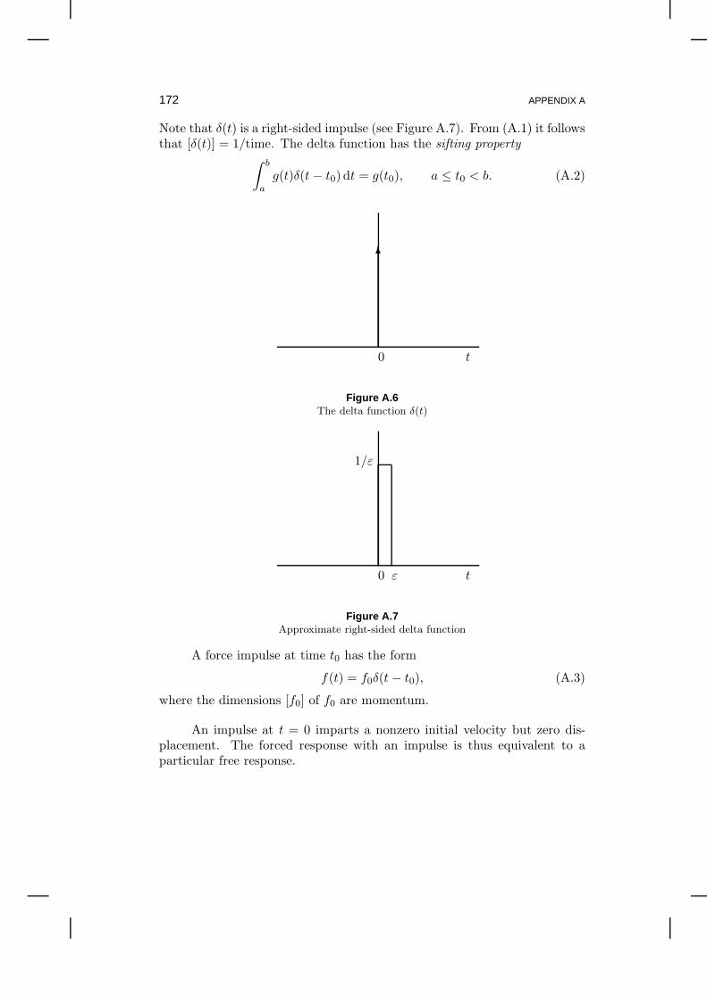
172 APPENDIX A
Note that δ(t) is a right-sided impulse (see Figure A.7). From (A.1) it followsthat [δ(t)] = 1/time. The delta function has the sifting property
∫ b
ag(t)δ(t − t0) dt = g(t0), a ≤ t0 < b. (A.2)
6
0 t
Figure A.6The delta function δ(t)
0 ε
1/ε
t
Figure A.7Approximate right-sided delta function
A force impulse at time t0 has the form
f(t) = f0δ(t− t0), (A.3)
where the dimensions [f0] of f0 are momentum.
An impulse at t = 0 imparts a nonzero initial velocity but zero dis-placement. The forced response with an impulse is thus equivalent to aparticular free response.

MATHEMATICAL BACKGROUND 173
6
0 t0 t
Figure A.8The delta function δ(t − t0)
Definition A.9.2 The function 1(t) is a unit step function, where
1(t)
=
0, t < 0,1, t ≥ 0.
0
1
t
Figure A.9The unit step function 1(t)
Definition A.9.3 The function
f(t) = f0t1(t) (A.4)
is a ramp.
Definition A.9.4 The function
f(t) = f0 sin (ωt+ φ) (A.5)
is a sinusoid.

174 APPENDIX A
0 t0 t
Figure A.10The unit step function 1(t − t0)
0 t
Figure A.11The ramp function
A.10 Laplace Transforms
q(s)
= Lq(t)
=
∫∞
0e−stq(t) dt. (A.1)
Note that [q(s)] = time× [q(t)] and [s] = 1/time. From (A.1) it follows that
Lq(t) =
∫∞
0e−stq(t) dt
= e−stq(t)∣∣∞
t=0+ s
∫∞
0e−stq(t) dt
= sq(s) − q(0).
Similarly,
Lq(t) = s2q(s) − sq(0) − q(0).

MATHEMATICAL BACKGROUND 175
Note that
Lδ(t) =
∫∞
0e−stδ(t) dt = e0 = 1.
L1(t) =
∫∞
0e−st1(t) dt =
∫∞
0e−st dt = −1
se−st
∣∣∣∣
∞
0
=1
s.
L
∫ t
0q(τ) dτ
=1
sLq(t).
Leat
=1
s+ a.
L sin(ωt) = L
1
2
[eωt − e−ωt
]
=1
2
[1
s− ω− 1
s+ ω
]
=1
2
2ω
s2 + ω2
=ω
s2 + ω2. (A.2)
L cos(ωt) = L
1
ω
d
dtcos(ωt)
=1
ωs
ω
s2 + ω2
=s
s2 + ω2. (A.3)
Note that
L cos(0t) =s
s2 + 02=
1
s= L 1(t) .
J.1 Time delay
The Laplace transform of a time delay is given by
Ly(t− τ) = e−τsy(s). (A.4)
176 APPENDIX A
J.2 s-shift
An s-shift in the Laplace transform is represented in the time domainas
Le−aty(t) = y(s+ a). (A.5)
Hence
L−1y(s+ a) = e−aty(t) (A.6)
and
L−1y(s− a) = eaty(t). (A.7)
Example A.10.1
Le−at sin(ωt) =ω
(s+ a)2 + ω2.
J.3 Time multiplication
Lty(t) = −y′(s). (A.8)
Hence,
L−1y′(s) = −ty(t),
which is the dual of
Ly(t) = sy(s) − y(0). (A.9)
A.11 Solution of ODE’s
Taking the Laplace transform of
q(t) + q(t) = 0
yields
Lq(t) + Lq(t) = 0.
Therefore,
s2q(s) − sq(0) + q(0) + q(s) = 0
and
q(s) =sq(0)
s2 + 1+
q(0)
s2 + 1.

MATHEMATICAL BACKGROUND 177
Hence,
q(t) = q(0) cos(t) + q(0) sin(t).
Example A.11.1 Consider the differential equation
q(t) = − c
mq(t) − k
mq(t) +
f(t)
m.
Taking the Laplace transform yields
q(s) =mq(0)s + cq(0) +mq(0)
ms2 + cs+ k︸ ︷︷ ︸
free response
+1
ms2 + cs+ k︸ ︷︷ ︸
forced response
f(s).
Definition A.11.1 A zero of a rational function is a root of the numer-ator of the rational function. A pole of a rational function is a root of thedenominator of the rational function.
Example A.11.2 Consider the forced response of the damped rigidbody
q(t) + 2q(t) = u(t).
If u(t) = δ(t), then the displacement is given by
q(s) =1
s2 + 2s.
Define the velocity v(t) = q(t). Then
v(t) + 2v(t) = u(t).
Now, if u(t) = 1(t), then the velocity is given by
v(s) =1
s(s+ 2).
Therefore, the displacement impulse response is identical to the velocityresponse.
K.1 Partial Fractions
Example A.11.3 Consider
y(s) =(s+ 2)(s + 4)
s(s+ 1)(s + 3).
Use partial fractions to show
y(t) =8
31(t) − 3
2e−t − 1
6e−3t.
178 APPENDIX A
A.12 Initial Value and Slope Theorems
The following result is the initial value theorem.
Fact A.12.1
y(0+) = lims→∞
sy(s)
The following result is the initial slope theorem.
Corollary A.12.1
y(0+) = lims→∞
s[sy(s) − y(0)]
Example A.12.1 If y(t) = 1(t), then
y(0+) = lims→∞
s1
s= 1.
If y(t) = cos(ωt), then
y(0+) = lims→∞
ss
s2 + ω2= 1.
Example A.12.2 Consider the unit-slope ramp
y(t) = t.
Then
y(0+) = lims→∞
s[sy(s) − y(0)]
= lims→∞
s(s1
s2− 0)
= 1.
A.13 Final Value Theorem
We say that limt→∞ y(t) exists if it is a number. Note that ∞ is nota number.
Case I y(t) remains bounded but limt→∞ y(t) does not exist. For example,y(t) = sin(ωt).
Case II y(t) is not bounded and thus limt→∞ y(t) does not exist. For ex-ample, y(t) = et sin t.
Case III y(t) is not bounded and limt→∞ y(t) does not exist but is infinite.For example, y(t) = et. In this case, limt→∞ y(t) = ∞.

MATHEMATICAL BACKGROUND 179
Case IV limt→∞ y(t) exists.
The following result is the final value theorem.
Theorem A.1. Every pole of y(s) is either in the open left half planeor is zero if and only if
limt→∞
y(t) = lims→0+
sy(s). (A.1)
In addition, limt→∞ y(t) exists if and only if s = 0 is not a repeated pole ofy(s).
The cases in Theorem A.1. are legal. For all other cases the final valuetheorem gives the wrong answer.
Example A.13.1 If y(t) = 1(t), then
limt→∞
y(t) = lims→0+
s1
s= 1.
If y(t) = −t1(t), then
limt→∞
y(t) = lims→0+
s1
s2= −∞.
If y(t) = e−t, then
limt→∞
y(t) = lims→0+
s1
s+ 1= 0.
If y(t) = et, then
limt→∞
y(t) = lims→0+
s1
s− 1= −1,
which is incorrect. Note that s → 0+ is needed in the second example toobtain the correct sign of ∞ when there is an odd number of repeated polesat s = 0.
A.14 Laplace Transforms of State Space Models
Consider
x(t) = Ax(t) +Bu(t),
y(t) = Cx(t) +Du(t).
Then
sx(s) − x(0) = Ax(s) +Bx(s),
y(s) = Cx(s) +Du(s).

180 APPENDIX A
Hence,
y(s) = C(sI −A)−1x(0)︸ ︷︷ ︸
free response
+
G(s)︷ ︸︸ ︷[C(sI −A)−1B +D
]u(s)
︸ ︷︷ ︸
forced response
.
G(s) thus has the realization
G(s) ∼[A BC D
]
.
We write
G(s) = C(sI −A)−1B +D
=1
sC
(
I − 1
sA
)−1
B +D
=1
sC
[
I +1
sA+
1
s2A2 + · · ·
]
B +D
= D +1
sCB +
1
s2CAB + · · ·
= H0 +1
sH1 +
1
s2H2 + · · · , (A.1)
where H0, H1, and H2 are Markov parameters. Note that the expansion(A.1) of G(s) converges if |s| >> 1.
G(s) is a ratio of polynomials in s, for example,
G(s) =as3 + · · ·s3 + · · · . (A.2)
Taking the limit of G(s) we obtain
a = lims→∞
G(s) = D. (A.3)
In the case D = 0, G(s) is of the form
G(s) =as2 + · · ·s3 + · · · , (A.4)
and thus
a = lims→∞
sG(s) = CB. (A.5)
Furthermore, if D = 0 and CB = 0, then G(s) is of the form
G(s) =as+ · · ·s3 + · · · , (A.6)

MATHEMATICAL BACKGROUND 181
and thus
a = lims→∞
s2G(s) = CAB. (A.7)
Example A.14.1 Consider the differential equation for the dampedoscillator
q(t) = − c
mq(t) − k
mq(t) +
f(t)
m.
Define the state variables x1(t)
= q(t) and x2(t)
= q(t) and assume that thevelocity q(t) is the output. Then
[x1(t)x2(t)
]
=
[0 1
− km − c
m
] [x1(t)x2(t)
]
+
[01m
]
f(t),
y(t) =[
0 1][x1(t)x2(t)
]
,
and
G(s) =[
0 1]([
s 00 s
]
−[
0 1
− km − c
m
])−1 [
01m
]
=s
ms2 + cs+ k.
Every pole of G(s) is an eigenvalue of A. In addition, in most casesevery eigenvalue of A is a pole of G(s). As an exception, consider theDRB with velocity output y(t) = v(t) = q(t). Then the eigenvalues of
A =
[0 10 − c
m
]
are λ1 = 0 and λ2 = − cm . Also,
y(s) = v(s) =s
s2 + cms
=1
s+ cm
. (A.8)
The pole at 0 is canceled by the zero at 0 since the position state is unob-servable by the velocity measurement.
A.15 Pole Locations and Response

182A
PP
EN
DIX
A
Open Left Half Plane (OLHP) Imaginary Axis (IA) Open Right Half Plane (ORHP)
not repeated ce−at sin(ωt)
repeated cte−at sin(ωt)
not repeated sin(ωt)
repeated t sin(ωt)
not repeated ceat sin(ωt)
repeated cteat sin(ωt)
not repeated ce−at
repeated cte−at
not repeated c
repeated ct
not repeated ceat
repeated cteat
not repeated ce−at sin(ωt)
repeated cte−at sin(ωt)
not repeated sin(ωt)
repeated t sin(ωt)
not repeated ceat sin(ωt)
repeated cteat sin(ωt)

MATHEMATICAL BACKGROUND 183
Consider the transfer function
G(s) =1
s2 + 2ζωns+ ω2n
. (A.1)
If ζ ≥ 1, then the roots of the characteristic equation are
λ1, λ2 = −ζωn ± ωn
√
ζ2 − 1.
If ζ > 1, then the roots are real and distinct, which is the overdamped case.If ζ is large, then λ1 ≈ −ωn/2ζ and λ2 ≈ −2ζωn. Thus λ2 is the faster poleand λ1 is the slower pole. For ζ = 1 the roots are repeated and given byλ = −ζωn, which is the critically damped case. For 0 < ζ < 1 the roots arecomplex, that is,
λ1, λ2 = −ζωn ± ωn
√
1 − ζ2,
which is the underdamped case. Defining the damped natural frequency
ωd = ωn
√
1 − ζ2, (A.2)
we have
λ1, λ2 = −ζωn ± ωd. (A.3)
Finally, if ζ = 0, then the roots are imaginary, which is the undamped case.
I
×
−ζωn
ωn
√
1 − ζ2
θ
ωn
Figure A.12Relationship between pole location, damping, and natural frequency
Notice that in the undamped, underdamped, and critically dampedcases we have
|λ| = ωn
and
ζ = sin θ.
Therefore, the distance from the pole to the origin determines the naturalfrequency, while the angle it subtends at the origin from the imaginary axis

184 APPENDIX A
Property Name Free Response
ζ = 0 undamped sinusoid
0 < ζ < 1 underdamped decaying sinusoid
ζ = 1 critically damped decaying exponentials
ζ > 1 overdamped decaying exponentials
Table A.2 Damping and free response.
determines the damping. Furthermore, the impulse response of the system(A.1) is given by
y(t) = e−ζωnt cos(ωn
√
1 − ζ2t+ φ).
Therefore the real part of the root determines the rate of decay, and theimaginary part determines the frequency of oscillation.
We summarize the various free responses in Table A.2.
A.16 Stability
Stability concerns the free response only. However, stability can alsobe determined from G(s).
Unstable
• x(t) → ∞ as t→ ∞ for at least one x(0).
• At least one entry of eAt is unbounded.
• Not Lyapunov stable.
• At least one pole of G(s) is in the ORHP or is repeated on theimaginary axis.
• Example: Undamped rigid body (URB).
Lyapunov Stability (LS)
• For all x(0), x(t) is bounded.
• Every entry of eAt is bounded.
• Each eigenvalue of A is in the OLHP or is not repeated on theimaginary axis.

MATHEMATICAL BACKGROUND 185
• Each pole of G(s) is in the OLHP or is not repeated on theimaginary axis.
• Example: UO.
Semistability (SS)
• For all x(0), limt→∞ x(t) exists.
• Each eigenvalue of A is in the OLHP or is not repeated at theorigin.
• limt→∞ eAt exists.
• Each pole of G(s) is in the OLHP or is not repeated at the origin.
• Example: DRB.
Asymptotic Stability (AS)
• For all x(0), x(t) → 0 as t→ ∞.
• Each eigenvalue of A is in the OLHP.
• limt→∞ eAt = 0.
• Each pole of G(s) is in the OLHP.
• Example: DO.
Fact A.16.1 AS =⇒ SS =⇒ LS
AS
SSLSUS
Figure A.13Stability Venn Diagram
Definition A.16.1 The transfer function G(s) is bounded-input,bounded-output (BIBO) stable if, for every bounded input signal u(t), theoutput y(t) of G(s) is bounded.

186 APPENDIX A
Example A.16.1 Consider the undamped rigid body
v(s) =1
msf(s)
with velocity output and force step input f(t) = f01(t). Then v(t) is un-bounded. Mathematically, v(t) is the integral of a step function. Physically,the velocity under nonzero constant forcing increases without bound. Hence
G(s) =1
ms
is not BIBO stable.
Example A.16.2 Consider the undamped oscillator with position out-put and sinusoidal force input f(t) = sinωnt. The output y(t) has repeatedpoles on the imaginary axis. The corresponding time-domain response,which is an oscillation with a linear envelope, is known as resonance. Hence
G(s) =1
s2 + ω2n
(A.1)
is not BIBO stable.
Fact A.16.2 G(s) is BIBO stable if and only if G(s) is asymptoticallystable.
A.17 Routh Stability Criterion
Fact A.17.1 Suppose that all of the roots of the polynomial
p(s) = sn + an−1sn−1 + · · · + a1s+ a0
are in the open left half plane. Then a0, . . . , an−1 are positive.
Fact A.17.2 Suppose that n = 2. Then both roots of
p(s) = s2 + a1s+ a0
are in the open left half plane if and only if a0 and a1 are positive.
Fact A.17.3 Suppose n = 3. Then all three roots of
p(s) = s3 + a2s2 + a1s+ a0
are in the open left half plane if and only if a0, a1, a2 are positive and
a0 < a1a2. (A.1)
Fact A.17.4 Suppose n = 4. Then all four roots of
p(s) = s4 + a3s3 + a2s
2 + a1s+ a0

MATHEMATICAL BACKGROUND 187
are in the open left half plane if and only if a0, a1, a2, a3 are positive and
a0a23 + a2
1 < a1a2a3. (A.2)
A.18 Problems
Problem A.18.1 Consider the 3 × 3 matrix
A =
3 0 24 3 57 2 6
.
Manually compute the determinant and inverse of A. Then compute thesequantities using Matlab to check your answer.
Problem A.18.2 Use Matlab to compute the eigenvalues of the matrixA in Problem A.18.1. Then use Matlab to show that the determinant is theproduct of the eigenvalues, and show that the trace (the sum of the diagonalentries) is the sum of the eigenvalues. Furthermore, use Matlab to computethe eigenvalues of A2 and A−1, and discuss how they are related to theeigenvalues of A.
Problem A.18.3 Using the “rand” command in Matlab, form a ran-dom 4 × 2 matrix A. Then compute the 4 × 4 matrix AAT. Using Matlabto compute the eigenvalues of AAT, check whether this matrix is positivesemidefinite. Then, show mathematically (by hand, not using Matlab) thatxTAATx ≥ 0 for all vectors x. (Hint: Define z = ATx.)
Problem A.18.4 Let A be an n×n matrix and let p(s) = det(sI −A)be the characteristic polynomial of A. The Cayley-Hamilton theorem statesthat p(A) = 0. Check this fact by obtaining the characteristic polynomialp(s) for the matrix
A =
[0 1
−a0 −a1
]
,
and then showing that p(A) = 0. Repeat these steps for
A =
0 1 00 0 1
−a0 −a1 −a2
.
Do all of these symbolic calculations by hand.
Problem A.18.5 The eigenvalues of a matrix are the roots of its char-acteristic polynomial. Consider the 3 × 3 matrix in Problem A.18.4 witha0 = −2, a1 = 5, and a2 = 3, and use Matlab to show numerically that theroots of p(s) are indeed the eigenvalues of A. Use roots(p) and eig(A) for

188 APPENDIX A
your computations.
Problem A.18.6 Show that the matrix
A =
[cos θ sin θ− sin θ cos θ
]
is orthogonal. Also, check whether the matrix
B =
[cos θ sin θsin θ − cos θ
]
is orthogonal. Determine by hand (not by Matlab) the determinants andeigenvalues of these matrices. Finally, choose several values of θ and applythese matrices to the vector [1 1]T. Discuss how the resulting vectorscompare to the original vector in terms of their length and direction. Youcan use a calculator but do not use Matlab.
Problem A.18.7 Use the dot product to compute the angle betweenthe vectors [3 2]T and [−2 4]T.
Problem A.18.8 Solve the differential equation
x(t) = ax(t) + b
analytically by evaluating the convolution integral expression given by (A.3)in Section A.8. Under what conditions does limt→∞ x(t) exist? When thelimit exists, determine the limiting value. How could you guess the limitingvalue without solving the equation?
Problem A.18.9 Using the solution to Problem A.18.8, write downthe solution to the scalar ordinary differential equation
x(t) = −2x(t) + 8.
This equation represents the step response of a linear system, where theconstant 8 is the value of the step input. Plot the solutions for the ini-tial conditions x(0) = 5 and x(0) = −4 in the same figure. Be sure tolabel all axes of your figure and give it an appropriate caption. Determinelimt→∞ x(t) from the plot and compare that numerical value with the ana-lytical limit. Explain how the limiting value of x(t) depends on the constantsin the problem, namely, the coefficient of x(t), the step value, and the initialcondition.
Problem A.18.10 Consider x = Ax, and let λ = σ+ ω be a complexvalue of A with associated complex eigenvector
v =
[31
]
+
[14
]
.
Let ω = 1 and σ = −1, 0, 1 (three different values), and plot the eigensolution

MATHEMATICAL BACKGROUND 189
x(t) = [x1(t) x2(t)]T = Re(eλtv) in the x1, x2 plane for each value of σ.
Explain how the properties of the eigensolution depend on σ.
Problem A.18.11 Let λ, λ = −ζωn ± ωn
√
1 − ζ2 denote a complexconjugate pair of underdamped eigenvalues. Show that
ωn = |λ|, (A.1)
ζ = −λ+ λ
ωn, (A.2)
and
ωd =λ− λ
2. (A.3)
Problem A.18.12 Let λ1, λ2 = −ζωn ± ωn
√
ζ2 − 1 denote a pair ofoverdamped eigenvalues. Show that
ωn =√
λ1λ2 (A.4)
and
ζ = − 1
ωn. (A.5)
Problem A.18.13 Consider the damped oscillator (DO) with acceler-ation output. Write this system in A,B,C,D form.
Problem A.18.14 Use the initial value theorem to determine the initialvalue of each of the following functions: y(t) = t, y(t) = t+ 1, y(t) = sin 2t,and y(t) = cos 2t.
Problem A.18.15 Use the initial value theorem to determine the initialslopes of the functions in the previous problem.
Problem A.18.16 Use Laplace transforms to analytically determinethe total response of v + 2v = sin 5t for an arbitrary initial conditionv(0). Then show that you can choose a special initial condition v(0) sothat the total response is exactly sinusoidal, that is, there is no transient(non-sinusoidal) component of the solution. Finally, confirm your answer byusing ODE45 to simulate the system with this special initial condition aswell as another initial condition.
Problem A.18.17 A motor with constant applied torque is modeledas the damped rigid body Jθ + cθ = τ01(t), where J is the load inertia, cis the viscous damping coefficient, and τ0 is the moment. The initial angleθ(0) and initial angular rate θ(0) are zero. Use Laplace transforms and thefinal value theorem to determine the terminal angular rate limt→∞ θ(t). Also

190 APPENDIX A
compute the same limit by using the time-domain solution obtained fromLaplace transforms.
Problem A.18.18 For
y(s) =1
s(s2 + s+ 1),
use partial fractions to show that
y(t) = 1(t) − e−1
2t cos
(√3
2t
)
− 1√3e−
1
2t sin
(√3
2t
)
.
Problem A.18.19 Consider an object falling under the force of gravity.Ignore drag and model the motion as an undamped rigid body. Use Laplacetransforms to express the displacement q(t) as a function of t, q(0), q(0),and g.
Problem A.18.20 A body with mass M is falling under the force ofgravity. Atmospheric drag is modeled by a dashpot coefficient D, so thatthe system is modeled as a damped rigid body. Assuming initial velocityv0, use Laplace transforms to find the velocity v(t) for t > 0. Then use thefinal value theorem to compute the terminal velocity limt→∞ v(t).
Problem A.18.21 Consider the damped rigid body with position out-put, and write it in state space form x = Ax. Then determine eAt by us-ing the fact that the Laplace transform of the matrix exponential eAt is(sI − A)−1. Next, determine limt→∞ eAt by using the expression for eAt aswell as by applying the final value theorem to each entry of (sI −A)−1. Usethis result to determine the free response of the damped rigid body withinitial displacement q(0), initial velocity q(0), and output y(t) given by themass position. What kind of matrix is limt→∞ eAt?
Problem A.18.22 For each of the transfer functions G(s) below withinput u and output y, determine whether the use of the final value theoremis legal, and, if so, use it to determine the limit of the output y(t) as t→ ∞.Explain why or why not the use of the final value theorem is legal in eachcase.
5a) G(s) =−5
s(s+ 7)2, u(t) = 3e−2t.
5b) G(s) =5
s− 3, u(t) = 71(t) − 3δ(t − 4.2).
5c) G(s) =−4
s2 + 2.4s + .3, u(t) = 6t2.

MATHEMATICAL BACKGROUND 191
Problem A.18.23 Consider the damped rigid body with ramp forceinput u(t) = t and velocity output. Use Laplace transforms and partialfractions to determine the forced response for t ≥ 0.
Problem A.18.24 An engineer has shown that the output response ofa new airframe developed for a UAV application is given by
y(t) = 2e−6t.
Use the initial value to determine y(t). (Note the two dots.) Check youranswer by computing y(t) directly. Note: You must use the initial valuetheorem. (Hint: I showed in class that
Ly(t) = s2y(s) − sy(0) − y(0).)
Problem A.18.25 For both systems described below (described by atransfer function and input) and without using a calculator or computer,determine whether the use of the final value theorem is legal, and, if so, usethe final value theorem to determine the limit of the output y(t) as t→ ∞.Explain why or why not the use of the final value theorem is legal in eachcase. If the limit exists, use Matlab to plot the response and confirm youranswer. (Hint: For plotting consider the Matlab functions IMPULSE andLSIM.)
a) G(s) =s2 − 1
s(3s3 + 2s2 + 4s + 5), u(t) = 2δ(t).
b) G(s) =1
s(s2 + 3s + 1), u(t) = −2e−t sin 2t.
Problem A.18.26 For the systems described below and without usinga calculator or computer, determine whether the use of the final value the-orem is legal, and, if so, use the final value theorem to determine the limitof the output y(t) as t → ∞. Explain why or why not the use of the finalvalue theorem is legal in each case. If the limit exists, use Matlab to plot

192 APPENDIX A
the response in order to confirm your answer.
a) The free response of the damped rigid body with initial displace-ment q(0), initial velocity q(0), and output y(t) given by the massposition. Obtain the limit symbolically. Then use Matlab to sim-ulate the system with the numerical values m = 3 kg, c = 4 kg/s,q(0) = 1 m, and q(0) = −2 m/s.
b) The forced response of a system whose transfer function is
G(s) =4s2 − 12s− 16
2s5 + 2s4 + 4s3 + 2s2 + s
with the impulsive input u(t) = 3δ(t− 1).
Problem A.18.27 Flight testing of a new aircraft reveals that it hasa pair of underdamped complex conjugate poles. Testing reveals that thetime to 50% decay is T seconds, while analytical modeling shows that theimaginary parts of the poles are ±ωd, where ωd > 0. Derive an expressionfor the damping ratio ζ in terms of T and ωd. Show that your expression forζ satisfies 0 < ζ < 1.
Problem A.18.28 Flight testing of a new aircraft reveals that it be-haves like an overdamped oscillator. Analytical models are used to deter-mine the value of ωn. Measurements show that the time to 50% decay is Tseconds. Derive an expression for the damping ratio ζ in terms of T and ωn.Finally, show that your expression for ζ satisfies ζ > 1.
Problem A.18.29 Without taking inverse Laplace transforms, sketchthe step response of the transfer function
G(s) =4s− 3
s2 + .8s + 4.
Be sure to qualitatively capture the direction of the step response for smallpositive time t as well as the settling behavior for large time t. What featuresdoes your sketch illustrate? Then use Matlab to plot the step response.
Problem A.18.30 Consider the eigenvalues of the matrix
A =
[0 1
−k/m −c/m
]
for the undamped (c = 0) and damped (c > 0) oscillators. Let k = 2.5 kg/s2
and m = 7 m. Plot the locations of the eigenvalues as ×’s in the complexplane for a range of values of c. Choose a range that includes undamped,

MATHEMATICAL BACKGROUND 193
underdamped, critically damped, and overdamped cases. For each value ofc, plot a “×” in the complex plane.
Problem A.18.31 Show analytically that the poles of the undamped,underdamped, and critically damped oscillators satisfy |λ1| = |λ2| = ωn.Furthermore, show that the poles of the overdamped oscillator satisfy λ1λ2 =ω2
n. Explain the meaning of these results in terms of the plot you made inthe previous problem.
Problem A.18.32 Consider the second-order state space (A,B,C,D)system with
A =
[0 1−2 −3
]
, B =
[01
]
, C =[
1 1], D = 0.
Determine the transfer function G(s) for this system. Show that G(s) isactually a first-order transfer function due to pole-zero cancelation. Finally,determine a first-order state space (A, B, C, D) system whose transfer func-tion is the same G. (Remark: Given a transfer function G we are usuallyinterested in a realization (A,B,C,D) of G of the lowest possible order, thatis, where the size of A is as small as possible.)


Appendix B
Frequency Response
B.1 Sinusoidal Gain and Phase Shift
Assume all sinusoids below have the same frequency. The sinusoids inFig. B.1 have different amplitudes but the same phase. In Fig. B.2, thesinusoids have the same amplitude but different phases.
B.2 Phase Angle as a Delay or Advance
Consider
f(t) = sin(ωt)
and
g(t) = sin(ωt+ φ),
where φ ∈ [−π, π] is the phase shift. To solve for the time shift, we solvefor ∆t from g(t) = 0. We obtain (see Fig. B.3)
sin(ω∆t+ φ) = 0
or,
∆t = −φω.
We thus have
g(t) = sin(ωt − ω∆t)
= sin(ω(t− ∆t)).
If φ > 0, then ∆t < 0, and thus g(t) is advanced relative to f(t). On theother hand, if φ < 0, then ∆t > 0, and thus g(t) is delayed relative to f(t).
Now consider
f(t) = α sin(ωt+ φ) (B.1)

196 APPENDIX B
0 5 10 15 20−2
−1.5
−1
−0.5
0
0.5
1
1.5
2
x
y
Figure B.1Sinusoids with same frequency but different amplitudes.
0 5 10 15 20−1
−0.8
−0.6
−0.4
−0.2
0
0.2
0.4
0.6
0.8
1
x
y
Figure B.2Sinusoids with same amplitude but different phases.

FREQUENCY RESPONSE 197
−4 −2 0 2 4 6 8−1
−0.8
−0.6
−0.4
−0.2
0
0.2
0.4
0.6
0.8
1
t
g
sin φ
∆ =− φ/ωt
Figure B.3Phase shift as a time delay.
and
g(t) = α sin(ωt + φ)
as shown in Fig. B.4. Now suppose that 0 < φ− φ ≤ 180. In this case, wesay that g(t) leads f(t) or f(t) lags g(t). Note that leading by more than180 is equivalent to lagging by less than 180.
0 5 10 15 20−1.5
−1
−0.5
0
0.5
1
1.5
x
y
g(t) f(t)
Figure B.4Sinusoids g(t) and f(t), where g(t) leads f(t).
We can express f(t) as the phasor
f(t) = Im αe(ωt+φ), (B.2)
which is shown in Fig. B.5. Leading and lagging are represented in Fig.B.6.

198 APPENDIX B
(ω + φ)
f(t)
Re
Im
ω + φ
eα
t
j t
Figure B.5Phasor representation.
B.3 Frequency Response Law for Linear Systems
Suppose that a sinusoidal input (such as a forcing) is applied to anasymptotically stable linear system. Then the output (response) of the sys-tem approaches sinusoidal motion whose frequency is the same as the inputfrequency. The limiting sinusoidal motion is called the harmonic steady stateresponse. Note, however, that the response does not have a “limit” in theusual mathematical sense since it does not approach a constant value.
The transient behavior of the system before its response reaches har-monic steady state depends on the poles and zeros of the system as well asthe initial conditions of the internal states.
The ratio of the amplitude of the harmonic steady state response to theamplitude of the sinusoidal input is equal to the magnitude of the transferfunction evaluated at the input frequency ω, that is, |G(ω)|, while the phaseshift of the harmonic steady-state response relative to the phase of the inputis given by the phase angle of the transfer function at the input frequency,that is, atan2(Im G(ω),Re G(ω)). Note that the harmonic steady-stateresponse leads the input if 0 < ∠G(ω) < 180, whereas the harmonic steady-state response lags the output if −180 < ∠G(ω) < 0
We thus have
u(t) = u0 sin(ωt + φ) (B.1)

FREQUENCY RESPONSE 199
lags
Re
Im
φ
φ^
leads
Figure B.6Phasor representation of leading and lagging sinusoids.
and
yhss(t) = |g(ω)|u0 sin(ωt+ φ+ ∠G(ω)).
B.4 Frequency Response Plots for Linear SystemsAnalysis
Assume that G(s) is asymptotically stable. As seen previously, if theinput u(t) is sinusoidal, that is,
u(t) = U cos(ωt), (B.1)
where U is the amplitude and ω is the frequency of the sinusoidal input,then the harmonic steady-state output is
yhss(t) = M(ω)U(ω) cos(ωt + φ(ω)), (B.2)
where M(ω) is the gain and φ is a phase angle, which satisfy
M(ω)eφ(ω) = G(ω). (B.3)
That is,
M(ω) = |G(ω)| (B.4)
and
φ(ω) = ∠G(ω). (B.5)
Plots of the gain M versus input frequency ω and of the phase angle

200 APPENDIX B
φ versus input frequency ω are the Bode frequency response plots. Theplot of gain versus frequency is the magnitude plot, while the plot of phaseangle versus frequency is the phase angle plot. It is convenient to expressthese plots using base 10 logarithmic scales for the gain and frequency. Inparticular, the gain is often scaled 20log10M , referred to as decibels (dB).
The Matlab command for plotting the Bode frequency response isBode(A,B,C,D), where A, B, C, D define the state equations for the lin-ear system with the desired input variable and the desired output variable.This function can also be used in the form Bode(n,d), where the vectors nand d represent the numerator and denominator polynomials of the transferfunction for the linear system with specified input and output variables.
The Bode frequency response plot can be constructed for all trans-fer functions G(s) whether or not G(s) is asymptotically stable, semistable,Lyapunov stable, or unstable. However, the gain and phase shift character-istics of G(s) have a harmonic steady-state interpretation only in the casethat G(s) is asymptotically stable.
Properties of the Bode frequency response plots include:
• The gain |G(ω)| is finite if and only if ω is not a pole of G.
• The DC gain is the gain at zero frequency; the DC phase angle iseither zero degrees or −180 degrees. In the Bode plot the DC gain isevident from the low frequency part of the magnitude plot.
• For a linear system with more poles than zeros, that is, n > m, thegain goes to zero as the frequency tends to infinity; in the Bode plot,the magnitude plot tend to negative infinity dB as the frequency tendsto infinity.
• Each local maximum corresponds to a pair of complex eigenvalues withdamping ratio less than
√2/2.
• The total change in the phase angle from low frequency to high fre-quency is given by (n−m)90, where n−m is the excess of poles overzeros.
• The frequency ωmco at which the gain is unity (or, equivalently, zerodB) is the magnitude crossover frequency. The phase margin is definedas
PM = 180 −G(ωmco). (B.6)
• The frequency ωpco at which the phase angle is 180 degrees is the phasecrossover frequency. The gain margin is defined as
GM = −20 log |G(ωpco)|. (B.7)

FREQUENCY RESPONSE 201
B.5 Circuits and Filters
A lowpass filter reduces noise at high frequency. From the impedancelaw, we have
V = IZ = ZI
or
I =V
Z.
Here Z = Z(s) is a transfer function.
Example B.5.1 Consider
Vin − Vout = RI
and
Vout =I
Cs=Vin − Vout
RCs. (B.1)
Solving for Vout in (B.1, we obtain(
1 +1
RCs
)
Vout =1
RCsVin
or
Vout =1
RCs+ 1Vin =
1RC
s+ 1RC
Vin.
Now, the current I is
I =Cs
RCs+ 1Vin.
Hence, at high frequency,
I =Cω
RCω + 1Vin(ω) ≈ 1
RVin(ω).
B.6 Bode Plot
Consider
G(s) =1
ms.
With s = ω, G(s) becomes
G(ω) =1
mω=
−mω
.

202 APPENDIX B
Hence
|G(ω)| =1
mω.
We plot 20log |G(ω)| versus log ω. We write
y = 20log |G(ω)|
= 20log
∣∣∣∣
1
mω
∣∣∣∣
= −20log |mω|= −20log |m| − 20log |ω|= −20x+ b, (B.1)
where x = log |m| and b = −20log |ω|.
B.7 Magnitude Crossover Frequency
Suppose |G(ωmco)| = 1 sec/kg. We use ωmco for magnitude crossover.Then
1
mωmco= 1
sec
kg−rad, (B.1)
ωmco =1
m
rad
sec. (B.2)
B.8 Phase of G(ω)
Consider
G(ω) =1
mω=
−mω
= − 1
mω. (B.1)
The magnitude of G(ω) is
|G(ω)| =1
mω(B.2)
with phase angle
∠G(ω) = −90. (B.3)
Figure B.7 represents the phase of G(ω) on the unit circle while Fig. B.8represented G(ω) on the Bode phase angle plot.

FREQUENCY RESPONSE 203
o
Im G(j )
Re G(j )ω
ω
270
mω1( )G(j ) = −j ω
−90
o
Figure B.7Phase angle representation on the unit circle.
−90
ω
ωG(j )
log
o
Figure B.8Phase angle representation on the Bode phase plot.
B.9 Poles at s = p
Consider
G(s) =α
s− p. (B.1)
Substituting s = ω, we obtain
G(ω) =α
ω − p. (B.2)
Note that if p < 0, then G is asymptotically stable, whereas, if p > 0, thenG is unstable. The magnitude of G(ω) is
|G(ω)| =|α|
√
ω2 + p2. (B.3)

204 APPENDIX B
For ω << p,
|G(ω)| =|α||p| (B.4)
while, for ω >> p,
|G(ω)| =|α||ω| . (B.5)
Now, for ω = |p|, the magnitude of G(ω) becomes
|G(|p|)| =|α|√
2p2=
√2
2
|α||p| . (B.6)
Hence, ∆dB is found from
∆dB = 20 log |G(|p|)| − 20 log |G(0)|
= 20 log
(√2
2
|α||p|
)
− 20 log
( |α||p|
)
= 20 log
(√2
2
)
= 20 log 2−1/2 = −10 log 2 = −3 dB. (B.7)
B.10 Phase Angle
Consider
z = a+ b (B.1)
as represented on Fig. B.9. To find the phase angle θ, we can write
tan θ =Im z
Re z. (B.2)
Consequently,
∠G(ω) = atan2(Im G(ω),Re G(ω)). (B.3)
The function atan2(a,b) is discussed in Appendix C.
B.11 Damped Oscillator
Consider
q(s) = G(s)f (s), (B.1)

FREQUENCY RESPONSE 205
z = a + jb
Im
Re
z = θ
Figure B.9Phase angle representation in the complex plane.
where
G(s) =1
ms2 + cs+ k
=1/m
s2 + 2ζωns+ ω2n
. (B.2)
Substituting s = ω, yields
G(ω) =1/m
−ω2 + 2ζωn(ω) + ω2n
=1/m
ω2n − ω2 + (2ζωnω)
=1/m[ω2
n − ω2 − (2ζωnω)]
(ω2n − ω2)2 + (2ζωnω)2
. (B.3)
B.12 Problems
Problem B.12.1 Consider the transfer function
G(s) =1
s2 + 2ζωns+ ω2n
with ωn = 1 rad/sec. Use Matlab to plot the magnitude and phase Bodeplots of this function for ω from .01 to 100 for ζ = .1, .3, .5, .7, .9. Put allplots in the same figure.
Problem B.12.2 Consider the transfer function
G(s) =1
s2 + 2ζωns+ ω2n
.

206 APPENDIX B
Assume that the system is underdamped, that is, 0 < ζ < 1. Use calculusto determine the resonance frequency ωr at which the magnitude |G(ω)|is maximized. Check whether your answer agrees with the figure from theprevious problem (B.12.1). In addition, determine the range of values of ζfor which the magnitude of the transfer function is never greater than itsDC, that is, ω = 0, value.
Problem B.12.3 Sketch Bode magnitude and phase plots AND theNyquist plot by hand for each of the following transfer functions. You canuse Matlab to print an “empty” log-log grid for your sketch. Be sure that therange of ω is large enough to include all important features of your plots.Explain how each plot was constructed. Check your sketches by plottingwith the Matlab Bode and Nyquist functions. Question: What is strangeabout the Nyquist plots that Matlab draws?
i) G(s) = s+2s+10 (lead).
ii) G(s) = s+10s+2 (lag).
iii) G(s) = s−2s+10 .
iv) G(s) = s−2s+2 (allpass).
v) G(s) = ss+2 (washout).
Problem B.12.4 For each of the following transfer functions, sketchthe Bode magnitude and phase plots by hand. You can use Matlab to printan “empty” log-log grid for your sketch. Be sure that the range of ω is largeenough to include all important features of your plots. Explain how eachplot was constructed. Check your sketches by plotting with Matlab.
i) G(s) = s2
(s+1)2(s+10)2 (rooftop).
ii) G(s) = (s+1)(s+100)s(s+5)(s+10) .
Problem B.12.5 Suppose that a sensor with first-order dynamics hasa time constant of .031 sec and a DC (that is, zero-frequency) magnitudeof 9.2. (Hint: G(s) = α
Ts+1 .) Now suppose that the input to the sensor is4.6 volts corrupted by (which means “added to”) 60 Hz electrical noise withamplitude 3.3 mV. Describe the sensor output after a large amount of timepasses by giving the amplitude and phase of all of its harmonic components.
Problem B.12.6 Suppose that a voltage amplifier with first-order dy-namics G(s) = α
Ts+1 has a time constant of T = 0.037 sec and DC gainα = 43.1. A sinusoidal input signal with amplitude of 2.8 volts yields, after

FREQUENCY RESPONSE 207
an initial transient, a sinusoidal response with amplitude 76.2 volts. Whatwere the frequencies of the input sinusoid and the output sinusoid?
Problem B.12.7 A lag filter has a pole at -2, a zero at -6, and a DCgain of 10. At the frequency 4 rad/sec, what is the magnitude of the filter indB and what is the phase angle of the filter in degrees? (Use just a calculatorfor this problem.)


Appendix C
MATLAB Operations
C.1 atan2
The MATLAB command atan2(y, x) computes the angle θ ∈ [−π, π]of the complex number x+ y.
Example C.1.1 For x = 1 and y = 1,
θ = atan2(y, x) = atan2(1, 1) =π
4.
For x = −1 and y = −1,
θ = atan2(−1,−1) =5π
4
. However, note that, in both cases, tan θ = 1.
C.2 expm
The MATLAB command expm(A) computes the exponential eA of thematrix A.
C.3 rlocus
The MATLAB command rlocus(n′, d′) if used for plotting the rootlocus of a transfer function where n′ and d′ are vectors that represent thepolynomials that define the numerator and the denominator of a character-istic polynomial. Specifically,
n′(s) = (s− z′1) · · · (s− z′m) (C.1)
is a polynomial of degree m and
d′(s) = (s − p′1) · · · (s− p′n) (C.2)
is a polynomial of degree n, with m ≤ n.

210 APPENDIX C
C.4 bode
The Matlab command for plotting the Bode frequency response isbode(A,B,C,D), where A, B, C, D define the state equations for the linearsystem with the desired input variable and the desired output variable. Thefunction can also be used in the form bode(n′, d′) where n′ and d′ are definedas in Section C.3.

Appendix D
Dimensions and Units
D.1 Mass and Force
For pound force,
1 lb = 1 slug-ft/sec2 = 4.4 N, (D.1)
where N denotes Newton. On the surface of the Earth, 1 kg weighs 9.8 N,while 1 slug weighs 32.2 lb. Conversion between slugs and kilograms is
1 slug = 14.59 kg. (D.2)
D.2 Force, Impulse, and Momentum
The impulse δ(t) has units
[δ(t)] = 1/sec. (D.1)
For the force impulse f(t) = f0δt, the coefficient f0 has the units
[f0] = [f(t)]/[δ(t)] = kg-m/sec (D.2)
which are the units of momentum. Specific impulse is given by f0/m whichhas the units
[f0/m] = m/sec, (D.3)
that is velocity.


Bibliography
[1] D. T. Greenwood, Advanced Dynamics, Cambridge University Press,Cambridge, 2003.
[2] P. C. Hughes, Spacecraft Attitude Dynamics, Wiley, New York, 1986.
[3] T. R. Yechout, Introduction to Aircraft Flight Mechanics, AIAA Edu-cation Series, VA, 2003.
[4] J. Roskam, Airplane Flight Dynamics and Automatic Flight Controls,DARCorporation, Lawrence, Kansas, 2001.
[5] R. C. Nelson, Flight Stability and Automatic Control, McGraw-Hill, 2ndEdition, 1997.
[6] R. F. Stengel, Flight Dynamics, Princeton University Press, 2004
[7] B. L. Stevens and F. L. Lewis, Aircraft Control and Simulations, Wiley-Interscience, 2nd Ed, 2003.
[8] D. G. Hull, Fundamentals of Airplane Flight Mechanics, Springer, 2007.