HAL Id: hal-01639731https://hal.inria.fr/hal-01639731

Submitted on 20 Nov 2017

HAL is a multi-disciplinary open accessarchive for the deposit and dissemination of sci-entific research documents, whether they are pub-lished or not. The documents may come fromteaching and research institutions in France orabroad, or from public or private research centers.

L’archive ouverte pluridisciplinaire HAL, estdestinée au dépôt et à la diffusion de documentsscientifiques de niveau recherche, publiés ou non,émanant des établissements d’enseignement et derecherche français ou étrangers, des laboratoirespublics ou privés.

Aircraft Dynamics Identification for Optimal ControlCédric Rommel, Joseph Frédéric Bonnans, Baptiste Gregorutti, Pierre

Martinon

To cite this version:Cédric Rommel, Joseph Frédéric Bonnans, Baptiste Gregorutti, Pierre Martinon. Aircraft DynamicsIdentification for Optimal Control. 7th European Conference on Aeronautics and Space Sciences(EUCASS 2017), Jul 2017, Milan, Italy. �10.13009/EUCASS2017-179�. �hal-01639731�

Aircraft Dynamics Identification for Optimal

Control

J. F. Bonnans1,2, B. Gregorutti3, P. Martinon1,2 and C. Rommel1,2,3

INRIA1, CMAP2, Safety Line3

cedric.rommel@safety-line.fr · frederic.bonnans@inria.frbaptiste.gregorutti@safety-line.fr · pierre.martinon@inria.fr

Abstract

Four new Maximum Likelihood based approaches for aircraft dynamicsidentification are presented and compared. The motivation is the need ofaccurate dynamic models for minimizing aircraft fuel consumption usingoptimal control techniques. A robust method for building aerodynamicmodels is also suggested. All these approaches were validated using realflight data from 25 different aircraft.

1 Introduction

Aircraft dynamics identification has been a longstanding problem in aircraftengineering, and is essential today for the optimization of flight trajectories inaircraft operations. This motivates the search for accurate dynamical systemsidentification techniques, the main topic of this paper. The application we aremost interested in here is aircraft fuel consumption reduction. It is known thatthis is as a major goal for airlines nowadays, mainly for economic reasons, butalso because it implies less CO2 emissions. We limit our study to civil flights,and more specifically to the climb phase, where we expect to have more room forimprovement. The techniques presented hereafter are suited for data extractedfrom the Quick Access Recorder (QAR). They contain multiple variables suchas the pressure altitude and the true airspeed, with a sample rate of one second.According to the literature [8, 11], two widely used approaches for aircraftdynamics estimation are the Output-Error Method and Filter-Error Method,based on the main ideas of measurement error minimization and state dynam-ics re-estimation. Recent advances include using neural networks for the stateestimation part [14]. On the other hand, renewed interest for the older Equation-Error Method has also been observed [12]. We propose in this paper variationsof the latter. Adopting a statistical point of view, we state several regressionformulations of our problem and solve them using Maximum Likelihood basedtechniques. We illustrate our methods with numerical results based on real datafrom 10 471 flights.

Organization of the paper: In section 2 we give a more detailed descriptionof the dynamics identification problem. The parametric models used in our

1

analysis are presented in section 3 and the estimation approaches tested aredescribed in section 4. Finally, section 5 contains the numerical results obtained.

2 Problem description

We consider an aircraft in climb phase, modeled as a dynamical system of statevariables x = (h, V, γ,m) ∈ X and control variables u = (α,N1) ∈ U (see table1 for the notations), where U = L∞(0, tf ;R2) and X = W 1,∞(0, tf ;R4) (i.e. theset of primitives of functions in L∞(0, tf ;R4)). In such a context, the problemof optimizing the trajectory during a certain horizon tf > 0 may be seen as anonlinear constrained optimal control problem of the following form:

min(x, u)∈X×U

∫ tf

0

`(t,u,x)dt+ ϕ(x(0),x(tf )),

s.t.

x = g(t,u,x), for a.e. t ∈ [0, tf ];u(t) ∈ Uad, for a.e. t ∈ [0, tf ],Φ(x(0),x(tf )) ∈ KΦ,cj(t,x(t)) ≤ 0, j = 1, . . . , nc, for all t ∈ [0, tf ].

(1)

All the mappings from (1), i.e. the running cost `, the final cost ϕ, the stateequation function g, the initial-final state constraint function Φ and state pathconstraints cj for j = 1, . . . , nc, are C∞. The set Uad is assumed to be a closedsubset of R2, KΦ is assumed to be a nonempty closed convex set of RnΦ andnΦ, nc ∈ N.

Table 1: Variables nomenclature

Notation Meaningh Aircraft altitudeV Aircraft true airspeed (TAS)γ Path anglem Aircraft massα Angle of attack (AOA)N1 Engines turbofan speedρ Air densityM Aircraft Mach numberSAT Static air temperatureθ Pitch angleC Total fuel flowT Total thrust forceD,L Drag and lift forcesCsp Specific consumptionψ Heading angleµ Bank angle (around TAS)W, ξ Wind speed norm and heading angle

Wx,Wy,Wz Horizontal and vertical wind speed components

2

The function g from (1) reflects the fact that we want the optimized trajec-tory to respect some model of the aircraft dynamics. A model of flight mechanicswhich can be used for this purpose is:

h = V sin γ +Wz,

V =T cosα−D −mg sin γ −mWxv

m,

γ =(T sinα+ L) cosµ−mg cos γ −mWzv

mV,

m = −CspT,

(2)

(3)

(4)

(5)

where Wxv = Wx cosψ cos γ + Wy sinψ cos γ + Wz sin γ,

Wyv = −Wx sinψ + Wy cosψ,

Wzv = −Wx cosψ sin γ − Wy sinψ sin γ + Wz cos γ.

(6)

In the previous system, Wx,Wy,Wz denote the horizontal and vertical windspeeds in the ground frame of reference and µ, ψ the bank and heading angles(see notations in table 1). Such dynamics account for variable wind duringthe flight as well as turning maneuvers. Several possibilities can emerge fromequations (2)-(5), by setting µ, ψ and/or Wx,Wy,Wz to zero. In this article weshall compare two of them: one obtained when µ = Wz = Wy = Wx = ψ = 0,called hereafter no-wind-dynamics, and the other one when just µ = Wz = 0,called wind-dynamics. Note that the models presented in section 3 stay the samefor both dynamics, as well as all identification processes described in section 4.In system (2)-(5), the elements T , D, L and Csp (see table 1 for notations) areunknown and assumed to be functions of the state and control variables. Itis quite common in flight mechanics to assume the following dependencies forthem, based on physical considerations:

T function of M,ρ,N1,

D function of M,ρ, α, V,

L function of M,ρ, α, V,

Csp function of M,h, SAT.

(7)

More details on these dependencies and their origins are discussed in section3.1. Now, given an aircraft for which a sufficient amount of flight data is avail-able, we aim to identify with the highest precision possible some model of itsdynamics, which is equivalent to estimate the four functions from (7). We insistthat our intention is to get customized dynamics for each individual aircraft,as opposed to one general model for a whole class of airplanes. Among manydifferent variables recorded in the QAR, nine of them seem sufficient for whatwe intend to do: h,M,C,N1, SAT, θ, ψ,W and ξ (see table 1 for notations).All other variables needed are derived from these ones using physical models ofcommon use in flight mechanics and presented in appendix A and B.

3

3 Parametric models

3.1 Models structure

As stated in paragraph 2, the thrust T , the specific consumption Csp, the dragD and the lift L are assumed to be functions of some physical variables listed in(7). In order to apply parametric identification methods to infer such functions,we need to assume that they belong to some parametrized function space. Thisis equivalent to choosing the form of the models. For the sake of simplicity,we choose to use linear identification models. In the case of the thrust and thespecific consumption, our models were inspired by [15, Chapter 2.2.1]:

T (M,ρ,N1) = N1ρ0.6(θT1 M

3 + θT2 ), (8)

Csp(M,h, SAT ) = θcsp1 h+ SAT12 (θcsp2 + θcsp3 h+ θcsp4 M + θcsp5 hM), (9)

where θT1 ,θT2 , . . .θ

csp5 are parameters to be estimated. Models (8)-(9) may be

rewritten so to make linearity explicit:

T = XT · θT , with

{XT = N1ρ

0.6[M3, 1]>,

θT = [θT1 ,θT2 ]>,

(10)

Csp = Xcsp·θcsp, with

{Xcsp = [h, SAT

12 , SAT

12h, SAT

12M,SAT

12hM ]>,

θcsp = [θcsp1 , . . . ,θcsp5 ]>.(11)

Concerning the aerodynamic forces, we use the common modelL(M,ρ, V, α) = 12ρV

2SCz(α,M),

D(M,ρ, V, α) = 12ρV

2SCx(α,M),(12)

where S is the wing planform area, Cx is the drag coefficient and Cz is the liftcoefficient. Ignoring the value of S, we model the products SCx and SCz asaffine functions of a family of monomials derived from the couple of variables(α,M). The technique used to select these monomials is described in the nextparagraph.

3.2 Aerodynamic features selection

Let d ∈ N such that d > 1. We consider a family of monomials of degree atmost d of the couple of variables (α,M):

X = (X1, . . . , Xr) =(αkM j−k : j = 0, . . . , d ; k = 0, . . . , j

)= (1,M, α,Mα, . . . ),

(13)

where r =

(d+ 2

2

). We assume hereafter that SCx and SCz are linear on

X: {Yx = SCx(α,M) = X · θD + εx,

Yz = SCz(α,M) = X · θL + εz,(14)

4

where · denotes the standard dot product in Euclidean spaces, θD,θL denotethe vectors of parameters and εx, εz are error terms. Let us assume now thatX,Yx, Yz, εx and εz are random variables. We have access to some observationsof X: {x1, . . . , xN}. Assuming Csp to be a known function of M,h, SAT (seesection 4.1), we are able to reconstruct observations of Yx and Yz from themeasured data, denoted respectively {yxi }Ni=1 and {yzi }Ni=1.

Performing the estimation of the parameters using all monomials throughlinear least-squares could lead to overfitting (see e.g. [7, Chap. 7.2]). There-fore, we search for a sparse structure of the parameter vectors θD,θL, which iscommonly known in statistics and machine learning as feature selection.

Given the linearity of model (14), a very popular feature selection methodis the Lasso [18]. It consists in using all possible variables to fit the availabledata through least-squares penalized by the L1-norm of the parameters vector:

minθ

N∑i=1

‖yi − xi · θ‖22 + λ‖θ‖1, (15)

where θ denotes either θD or θL and yi denotes either yxi or yzi for all i =1, . . . , N . This approach is known to be inconsistent when some of the variablesare highly correlated. Indeed, in this case, the variable selection is very sensitiveto the training data used. As some of the monomials in X are likely to becorrelated, we decided to use an adaptation of the Lasso which is supposed tobe consistent under such conditions: the Bolasso [2].

The idea of such feature selection technique is to perform the Lasso repeat-edly over several bootstrap replications of the initial data set, i.e. samples of sizeN drawn with replacement using a uniform distribution. The selected variablesare then given by the intersection of the variables selected over all Lasso execu-tions. This method has been proved to select the right variables with very highprobability under the following assumptions (believed to be verified here):

1. the cumulant generating functions E[exp(s‖X‖22)

]and E

[exp(sY 2)

]are

finite for some s > 0 (where Y denotes either Yx or Yz),

2. the joint matrix of second order moments E[XX>

]is invertible,

3. E [Y |X] = X · θ and V [Y |X] = σ2 a.s. for some θ ∈ Rr and σ ∈ R∗+.

The reader is referred to [2, section 3] for further details.Once the feature selection has been performed for both SCx and SCz, we

consider vectors containing the selected monomials only, denoted respectivelyXscx and Xscz, of length pD, pL ≤ r ∈ N∗. These new variables vectors will beused to determine the values of the parameters θD ∈ RpD and θL ∈ RpL , asexplained in section 4.

4 Estimation approaches

This section presents four possible identification methods of increasing complex-ity, all somehow derived from the wide Maximum Likelihood estimator. Theywill be compared to each other in section 5. For simplicity, all calculations inthis section will be based on the no-wind-dynamics, but the same approach canbe applied to the wind-dynamics.

5

4.1 Single-task Ordinary Least-Squares

The approach presented in this section is the most straightforward one. It willbe used as reference for comparison with all other approaches in the followingsections. Our first objective is to derive a set of regression problems from system(2)-(5) (where µ, ψ,Wx,Wy,Wz have all been set to 0 for simplicity).

We see that equation (2) does not contain any unknown element to be esti-mated, which means it is not useful here. While function T appears in (3)-(5),note that D, L and Csp take part in a single equation each. Equation (5) isclearly the problematic one, because of the presence of a product between theunknowns Csp and T . This means that we do not have linearity on the pa-rameters of the r.h.s. of this equations, but also that it cannot be used aloneto determine both elements separately: only the product of them is identifiablehere, in the sense of definition 4.1 (see e.g. [19, Chap 2.6.1]).

Definition 4.1 Identifiable modelLet M : Θ → Y be a model defined on some parameters space Θ into some

output space Y. M is said to be identifiable if for any θ1,θ2 ∈ Θ,

M(θ1) =M(θ2)⇒ θ1 = θ2. (16)

The simplest way of overcoming such difficulties is to choose not to inferCsp and use a general model of it instead. Even though this idea does notsolve the real problem, its simplicity led us to test it. For this, we chose thespecific consumption model from [15, Chapter 2.1.2], that we shall denote CERsphereafter. Thus, in this approach, only T,D and L are to be estimated basedon equations (3)-(5).

By isolating only a single unknown term in the right-hand side of each equa-tion, the system may be rewritten as follows:

−mV −mg sin γ +C

CERspcosα = D,

mV γ +mg cos γ − C

CERspsinα = L,

C

CERsp= T.

(17)

In system (17) we make two assumptions: (i) the mass rate m has been replacedby the negative total fuel flow −C and (ii) that T is assumed to be strictly equalto C/CERsp . Substituting the expressions of T , D and L in (10), (12) and (14),we build the following set of regression problems:

YD = XD · θD + θD0 + εD,

YL = XL · θL + θL0 + εL,

YT = XT · θT + θT0 + εT ,

(18)

with

6

YD = −mV −mg sin γ +C

CERspcosα,

YL = mV γ +mg cos γ − C

CERspsinα,

YT =C

CERsp, XD =

1

2ρV 2Xscx, and XL =

1

2ρV 2Xscz.

(19)

The intercepts θD0,θL0 and θT0, which are also estimated, should account forpossible offsets in the dynamics formulation, and εD, εL, εT are random variablesrepresenting the noise of in the models.

Remark Had we different assumptions for the dynamics of our aircraft, asdescribed in section 2, this would simply add some wind terms in (17) and (19),but would not change the structure of the problem.

We consider now only one of this regression problems taken separately, in-dexed by ` ∈ {D,L, T}. Given a sample

{(x`,1, y`,1), . . . , (x`,N , y`,N )

}drawn

independently, with N ∈ N, we rewrite the regression problem in its matrixform:

Y ` = X`θ` + ε`, (20)

with Y ` = [y`,1, . . . , y`,N ]>, ε` = [ε`,1, . . . , ε`,N ]> and X` = [x`,1, . . . , x`,N ].Note that each x`,i is a column vector of size p`. Also note that the interceptshave been included in the parameters vectors, by adding a column of ones to thematrices X`. We can then solve each of these regression problems separatelythrough Ordinary Least-Squares estimators:

θ` = (X>` X`)−1X>` Y `. (21)

Such estimator is quickly computed even in the case of large samples and,according to the Gauss-Markov Theorem (see e.g. [3, p.215]), it is the BestLinear Unbiased Estimator1 under the following assumptions:

• the covariates observations {x`,i, i = 1, . . . , N} are known (not drawn froma random variable);

• the noises have zero mean: E [ε`,i] = 0, for i = 1, . . . , N ;

• they are homoscedastic: V [ε`,i] = σ2 <∞, for i = 1, . . . , N ;

• and are mutually uncorrelated : Cov [ε`,i, ε`,j ] = 0, for any i 6= j.

Such assumptions are not all verified in practice. We know for example thatthere is some uncertainty in our covariates observations and that the autocor-relation between data points is quite significant. Considering this, extendedversions of this estimator may be better choices in our case, such as the Gen-eralized Least-Squares [1] or the Total Least-Squares (see e.g. [8, Chap 6.5]).These options, however, would still not allow us to infer Csp, which means wewould not be solving the initial problem. Problem (21) is solved using the func-tion linalg.lstsq from Python’s scipy.linalg library, which is based on theSVD decomposition of X` (see section 5.2).

1”Best” means of minimum variance here.

7

4.2 Multi-task nonlinear least-squares

As stated in section 4.1, two of the main difficulties of the identification problemtreated here are:

1. the non-identifiability (see definition 4.1) of the product of T and Csp inequation (5) and

2. the fact that T is present in (3)-(5), which means that we have no chanceof obtaining the same results three times if we used theses equations sep-arately to identify it.

These obstacles led us to use the three equations together, in a multi-task regres-sion framework [5]. The main idea here is that multi-task learning allows us toenforce all equations to share the same thrust function T , which solves difficulty2. By doing so, we expect information concerning T gathered while identifyingequations (3) and (4) will be somehow transferred to equation (5) during theestimation process, which should help to reduce the non-identifiability issue 1.

Unlike what was done in (17) for the Single-task Ordinary Least-Squares,here we will leave T in the r.h.s. of equations (3)-(5), since we want to use allof them to estimate it:

mV +mg sin γ = T cosα−D,

mV γ +mg cos γ = T sinα+ L,

C = CspT.

(22)

As before, by injecting T , D, L and Csp as defined in (10)-(12) and (14), webuild the set of regression problems:

Y1 = X1 · θ1 + ε1,

Y2 = X2 · θ2 + ε2,

Y3 = (XT · θT )(Xcsp · θcsp) + ε3,

(23)

where

Y1 = mV +mg sin γ,

Y2 = mV γ +mg cos γ,

Y3 = C,

(24)

and

X1 =

[XT cosα−XD

], X2 =

[XT sinαXL

], θ1 =

[θTθD

], θ2 =

[θTθL

].

(25)

Remark In the third equation of (23), we can still add an intercept as in section4.1, but it cannot be view as an augmented vector X. In this case, we adaptthe strategy by fitting the centered targets {Yi = Yi− Yi}3i=1 without interceptsand setting them a posteriori to be equal to the targets means {θi0 = Yi}3i=1.

8

As previously explained, we will consider the three regression problems from(23) as a single one, called multi-task regression problem

Y = f(X,θ) + ε, (26)

where

Y = [Y1, Y2, Y3]>, ε = [ε1, ε2, ε3]> ∈ R3, (27)

X = [XT , Xcsp, XL, XD]> ∈ Rm, θ = [θT ,θcsp,θL,θD]> ∈ Rp. (28)

Note that, for any x ∈ Rm, function f(x, ·) : θ 7→ f(X,θ) is nonlinear. We willcall hereafter a task each regression problem from system (23). The number oftasks solved by a multi-task regression is hence given by the dimension of theoutputs vector Y .

Now let us consider a certain training set {(xi, yi)}Ni=1 drawn from the jointdistribution of the random variables X,Y defined in (28) and (27). In order tosolve problem (26) we choose here to use the least-squares estimator once again:

θ ∈ arg minθ∈Rp

N∑i=1

‖yi − f(xi,θ)‖22. (29)

Problem (29) is an unconstrained non-convex optimization problem. It wassolved using the Levenberg-Marquardt algorithm implemented in the leastsqfunction from Python’s scipy.optimize library (see section 5.2).

4.3 Multi-task maximum likelihood

In this section we will present a different approach than the least-squares forsolving the multi-task regression problem (26). It differs from the previous oneby trying to leverage the correlation between the noises of the different tasks.Let us assume here for more generality that we are dealing with K ∈ N∗ tasks,i.e. Y, ε ∈ RK . Considering a training set {(xi, yi)}Ni=1, we are assuming throughour regression model that there is some θ ∈ Rp such that, for any i = 1, . . . , N

yi = f(xi,θ) + εi. (30)

We assume here that the εi are drawn independently from the same distributionN (0,Σ) for every i = 1, . . . , N . Then, for a given θ ∈ Rp, the samples likelihoodwrites

LML(θ,Σ) =

N∏i=1

[(2π)K det Σ]−12 exp

(−1

2ei(θ)>Σ−1ei(θ)

), (31)

where ei(θ) = yi − f(θ, xi) ∈ RK denotes the residue’s ith component. TheLog-Likelihood criterion is in this case

logLML(θ,Σ) = −NK2

log(2π)− N

2log det Σ− 1

2

N∑i=1

ei(θ)>Σ−1ei(θ). (32)

If we knew the covariance matrix Σ, the Maximum Likelihood estimatorunder such assumptions would be obtained by maximizing criterion (32) with

9

relation to θ, which is equivalent to solving the following weighted least-squaresproblem:

minθ

N∑i=1

ei(θ)>Σ−1ei(θ). (33)

Remark It becomes clear through expression (33) that, under the assumptionthat the K tasks have mutually independent noises of same variance σ (i.e.Σ = σIK , with IK the K×K Identity matrix), our new estimator is equivalentto the multi-task nonlinear least-squares estimator from section 4.2.

As we do not know Σ in our case, we will try to add it as a variable in ouroptimization problem, which becomes (after eliminating the constant term):

minθ,Σ

J(θ,Σ) =N

2log det Σ +

1

2

N∑i=1

e>i Σ−1ei. (34)

First order optimality condition with relation to Σ gives ∂

∂ΣJ(θ,Σ) = 0K where0K is the K ×K zero matrix and

∂

∂ΣJ(θ,Σ) =

N

2

∂

∂Σ(log det Σ) +

1

2

N∑i=1

∂

∂Σ

(e>i Σ−1ei

)(35)

=N

2Σ−1 − 1

2

N∑i=1

Σ−1eie>i Σ−1 =

1

2Σ−1

(NIK −

[N∑i=1

eie>i

]Σ−1

).

(36)

See e.g. [6, p.263] for further details. This leads to the classic covarianceestimator

Σ =1

N

N∑i=1

eie>i =

1

N

N∑i=1

(yi − f(θ, xi)

)(yi − f(θ, xi)

)>. (37)

Using such estimator, we may note that

N∑i=1

e>i Σ−1ei = Tr

{(N∑i=1

eie>i

)Σ−1

}(38)

= N Tr(IK) = NK, (39)

which allows us to simplify our log likelihood criterion (34) into

minθJ(θ) = log det Σ(θ). (40)

Problem (40) is unconstrained and non-convex, as (29), but is also highlynonlinear and harder to solve. We solved it using Python’s function fmin slsqpfrom scipy.optimize library, where Σ has been constrained to be positive-definite. The following section presents an attempt to facilitate such an opti-mization task.

10

4.4 Cholesky maximum likelihood

We chose here to modify criterion J(θ) by computing the modified Cholesky

decomposition of Σ(θ) = LDL>, where L is a unit lower triangular matrix and

D is a positive diagonal matrix. We assume here that Σ is positive definite.This ensures that det Σ(θ) is the product of the diagonal terms of D, which arenon-negative:

det Σ(θ) =

K∏j=1

Djj . (41)

In practice, we limit the scope of search to a positive definite Σ, which ensuresthat is no Djj equal to zero.

Hence, optimization problem (40) becomes

minθ,L,D

K∑j=1

logDjj

such that

{Djj > 0, ∀j = 1, . . . ,K

Σ(θ) = LDL>,

(42)

where L and D are possible Cholesky decomposition matrices of Σ. Comparedto (40), this new problem is not unconstrained anymore and its unknowns lie in aspace of higher dimension. Hence, at first view, our new problem may seem morecomplex than the former, even though the objective function has been greatlysimplified in the process. However, (40) is a reduction of (42) and we believe,based on empirical experience, that reduced problems are often more difficultto solve. This motivated us to use criterion (42). The algorithm chosen to solveit was, once again, fmin slsqp from scipy.optimize library (see section 5.2).This algorithm, as well as the three previous ones, has a computation time foreach iteration which increases linearly with the size of the training sample.

5 Numerical experiments: application to flightdata

In this section we will compare all methods presented above on real flight data.The quality criteria chosen will be described in the first subsection. Those aredefined for a given data set of q > 0 flights.

5.1 Assessment criteria

Let us consider a certain estimator (e.g. one of those presented in section 4)

allowing to infer the parameters θ = [θT , θcsp, θL, θD]>. A leave-one-out basedmethod is defined here. The models are trained on q − 1 flights (the trainingflights). Then predictions are made on the remaining flight (the test flight),assumed here to have been recorded on the times t0 = 0, . . . , tn = tf . Thisallows to check if our estimator performs well on new data, which prevents usfrom considering overfitting as good performance. More precisely predictionsof T,Csp, L and D are built thanks to (10)-(12) and (14) and the estimated

11

parameters θ. Based on the chosen dynamics system (as for example (2)-(5)),

the states derivatives ˆx = [ˆh, ˆV, ˆγ, ˆm]> can be finally reconstructed. From a

regression point of view, we might assess a given estimator by computing themean squared error of the reconstructed state derivatives (see section 5.2) andestimator prediction for the test flight:

C1 =1

n+ 1

n∑k=0

‖xtk − ˆxtk‖2x. (43)

Here, ‖ � ‖x denotes a scaling norm which brings all the components of x andx to the same order of magnitude before applying the usual Euclidean normin R4. Based on the ideas of M. Stone [16], this criterion can be computedq times, by permuting the selected test flight. Averaging the value of C1 overall permutations leads to a new performance criterion. Such a technique iswell-known in statistics and machine learning as cross-validation.

The issue with the previous criterion is that it is static: the fact that theobservations from the test flight are time series does not reflect in it. However,as stated in section 2, the final objective of our approaches is to estimate anaccurate model of the aircraft dynamics in order to inject it in an optimalcontrol problem (1). For solving such a problem, the identified dynamic systemwill be integrated several times using different controls in order to look for theadmissible control sequence which minimizes the objective function of (1). Agood estimator, when reintegrating the flight dynamics with the controls fromthe recorded flight, should give a trajectory close to the actual one. Noting(xm,um) the measured state and control sequences of a given test flight, and x

the trajectory reintegrated with um, we can rate an estimator θ identified usingthe training flights by looking at the distance between the two state trajectories:

C2 =1

n+ 1

n∑k=0

‖xtk − xtk‖2x. (44)

In practice, we cannot use this approach for the quality assessment. Indeed,the small errors on the estimations of ˆx accumulate over the integration stepsleading systematically to integrated states which move away quite rapidly fromthe measured states. To counter such phenomena, we try to find, for a given testflight, a control sequence not very far from the measured one which can bringthe integrated state sequence as close as possible to the real state sequence.This idea can be written as the following optimization problem:

minu

∫ tf

0

(‖u(t)− um(t)‖2u + ‖x(u, t)− xm(t)‖2x

)dt (45)

The norm ‖ � ‖u is an analog of ‖ � ‖x, but scaling u and um. The mappingx : U×R→ R4 denotes the function used to compute the integrated states withsome control function u ∈ L∞(0, tf ;R2) and the states derivatives obtained

using θ. If we denote u∗ a solution of problem (45), we can compute thefollowing performance index:

C3 =1

n+ 1

n∑k=0

(‖xtk − x

∗tk‖2x + ‖utk − u∗tk‖

2u

), (46)

12

where

u∗tk = u∗(tk), x∗tk = x(u∗, tk), for tk = 0, . . . , tf . (47)

As C1, this last criterion can be cross-validated across all possible permutationsof the test flight.

5.2 Implementation details and data description

We compared the identification approaches described in section 4 using realQAR data. All data sets used contained raw measurements of (h,M,C,N1, SAT, θ, ψ,W, ξ).These have been smoothed using smoothing splines (see Appendix C) and thenused to compute a posteriori all the other variables needed (see AppendicesA and B). In particular, the differentiated variables, such as V and γ, werecomputed analytically using the derivatives of measurements smoothed usingsplines.

The models used for T,Csp, L and D were those presented in section 3.1.Were compared two different dynamics, which are the no-wind-dynamics andthe wind-dynamics, as defined in section 2. The feature selection for the modelsof L and D was carried out previous to the estimation approaches from section4, using a data set containing 10 471 flights of 25 different Boeing 737. Themaximum degree of the monomials selected was d = 3. Only the climb phase ofthe flights were used here, i.e. data corresponding to altitudes between FL100 =10 000 ft and the top of climb (cruise altitude), specific to each flight. Prior tothe application of the Bolasso (described in section 3.2), the data set was splitinto a model selection set - 33% of it - and a training set. The penalization pa-rameter λ in (15) was selected a single time for all the 128 bootstrap replicationsof the Bolasso using the model selection set only. For this, 100 values for λ werecompared using the mean square error in a 50-fold cross-validation scheme (seee.g. [7, Chap. 7.10]). Concerning the estimation part, we wanted to identifya single aircraft (B737). Hence, a subset of q = 424 flights was used for thispurpose, which corresponds to 334 531 observations (after outliers deletion).

In practice, the Lasso estimations needed for the feature selection partwere carried out using the Lasso and LassoCV functions of Python’s scikit-learn.linear model library [13]. The latter are based on a coordinate descentalgorithm to solve the optimization problem (15). Concerning the optimizationpart of the estimation approaches, they are all performed using functions ofPython’s scipy library [9], as listed in table 2. As the Linear Least Squares isthe only method which is not iterative, its solution was used to initialize theNonlinear Least Squares, whose solution was used to initialize the other twoappoaches. The optimization of problem (45) was performed using BOCOP[17, 4].

Table 2: Optimization algorithms used

Estimation approach Function used AlgorithmSingle-task Ordinary Least-Squares linalg.lstsq SVD decompositionMulti-task Nonlinear Least-Squares optimize.leastsq Levenberg-Marquardt

Multi-task Maximum Likelihood optimize.fmin slsqp Dieter Kraft’s SQP algorithm [10]Cholesky Maximum Likelihood optimize.fmin slsqp Dieter Kraft’s SQP algorithm [10]

13

5.3 Results

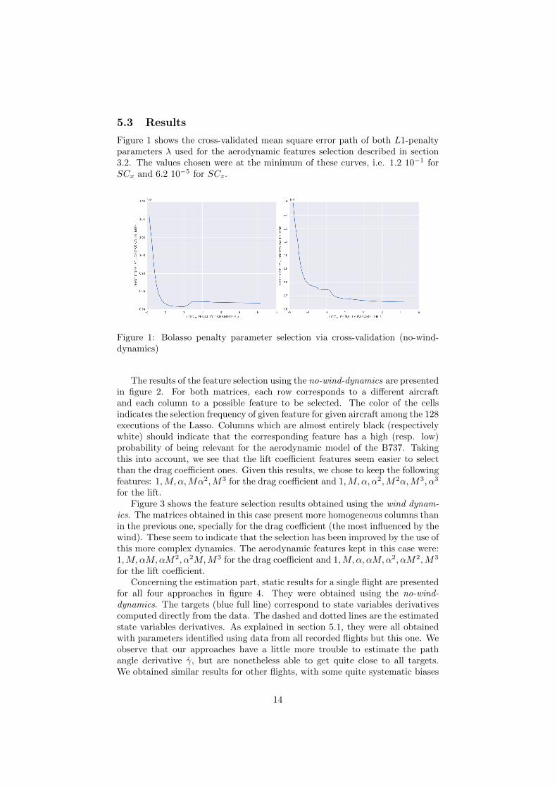
Figure 1 shows the cross-validated mean square error path of both L1-penaltyparameters λ used for the aerodynamic features selection described in section3.2. The values chosen were at the minimum of these curves, i.e. 1.2 10−1 forSCx and 6.2 10−5 for SCz.

Figure 1: Bolasso penalty parameter selection via cross-validation (no-wind-dynamics)

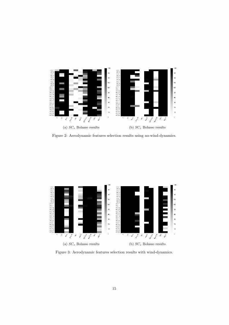
The results of the feature selection using the no-wind-dynamics are presentedin figure 2. For both matrices, each row corresponds to a different aircraftand each column to a possible feature to be selected. The color of the cellsindicates the selection frequency of given feature for given aircraft among the 128executions of the Lasso. Columns which are almost entirely black (respectivelywhite) should indicate that the corresponding feature has a high (resp. low)probability of being relevant for the aerodynamic model of the B737. Takingthis into account, we see that the lift coefficient features seem easier to selectthan the drag coefficient ones. Given this results, we chose to keep the followingfeatures: 1,M, α,Mα2,M3 for the drag coefficient and 1,M, α, α2,M2α,M3, α3

for the lift.Figure 3 shows the feature selection results obtained using the wind dynam-

ics. The matrices obtained in this case present more homogeneous columns thanin the previous one, specially for the drag coefficient (the most influenced by thewind). These seem to indicate that the selection has been improved by the use ofthis more complex dynamics. The aerodynamic features kept in this case were:1,M, αM,αM2, α2M,M3 for the drag coefficient and 1,M, α, αM,α2, αM2,M3

for the lift coefficient.Concerning the estimation part, static results for a single flight are presented

for all four approaches in figure 4. They were obtained using the no-wind-dynamics. The targets (blue full line) correspond to state variables derivativescomputed directly from the data. The dashed and dotted lines are the estimatedstate variables derivatives. As explained in section 5.1, they were all obtainedwith parameters identified using data from all recorded flights but this one. Weobserve that our approaches have a little more trouble to estimate the pathangle derivative γ, but are nonetheless able to get quite close to all targets.We obtained similar results for other flights, with some quite systematic biases

14

(a) SCx Bolasso results (b) SCz Bolasso results

Figure 2: Aerodynamic features selection results using no-wind-dynamics.

(a) SCx Bolasso results (b) SCz Bolasso results

Figure 3: Aerodynamic features selection results with wind-dynamics.

15

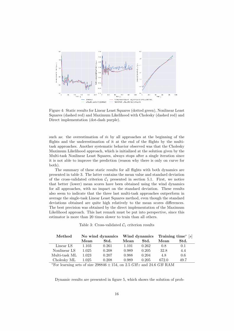
Figure 4: Static results for Linear Least Squares (dotted green), Nonlinear LeastSquares (dashed red) and Maximum Likelihood with Cholesky (dashed red) andDirect implementation (dot-dash purple).

such as: the overestimation of m by all approaches at the beginning of theflights and the underestimation of it at the end of the flights by the multi-task approaches. Another systematic behavior observed was that the CholeskyMaximum Likelihood approach, which is initialized at the solution given by theMulti-task Nonlinear Least Squares, always stops after a single iteration sinceit is not able to improve the prediction (reason why there is only on curve forboth).

The summary of these static results for all flights with both dynamics arepresented in table 3. The latter contains the mean value and standard deviationof the cross-validated criterion C1 presented in section 5.1. First, we noticethat better (lower) mean scores have been obtained using the wind dynamicsfor all approaches, with no impact on the standard deviation. These resultsalso seem to indicate that the three last multi-task approaches outperform inaverage the single-task Linear Least Squares method, even though the standarddeviations obtained are quite high relatively to the mean scores differences.The best precision was obtained by the direct implementation of the MaximumLikelihood approach. This last remark must be put into perspective, since thisestimator is more than 20 times slower to train than all others.

Table 3: Cross-validated C1 criterion results

Method No wind dynamics Wind dynamics Training time∗ [s]Mean Std. Mean Std. Mean Std.

Linear LS 1.103 0.261 1.101 0.262 0.8 0.1Nonlinear LS 1.025 0.208 0.989 0.205 32.8 4.4

Multi-task ML 1.023 0.207 0.988 0.204 4.8 0.6Cholesky ML 1.025 0.208 0.989 0.205 672.0 49.7∗For learning sets of size 298846± 154, on 2.5 GHz and 24.6 GB RAM

Dynamic results are presented in figure 5, which shows the solution of prob-

16

lem (45) for the same flight of figure 4. They were obtained using the no-wind-dynamics and allow to compare the single-task Linear Least Squares tothe multi-task Nonlinear Least Squares. Notice that the curves are plotted asfunctions of the altitude, which is possible since the latter is monotonic overthe climb phase. We see that the predicted dynamics were able to reproducequite accurately the recorded flight in this case with a minor correction on theangle-of-attack α and a 20% maximum correction on the engines speed N1. Sim-ilar results were obtained for other flights, which seems promising for the useof such techniques prior to optimal control problems. In addition, we observeonce again that the multi-task approach returns slightly better results than thesingle-task one. This has been confirmed by the results presented in table 4,which contains the mean value and standard deviation over all flights of thecross-validated criterion C3 from section 5.1.

Figure 5: Solution of problem (45) using dynamics estimated by Linear LeastSquares (dotted green) and Nonlinear Least Squares (dashed red), in comparisonto recorded flight (full blue line).

Table 4: Cross-validated C3 criterion results, with no-wind-dynamics

Method Mean Std.Linear LS 1.266 0.120

Nonlinear LS 1.245 0.168

6 Conclusion

We presented in this article four different versions of Maximum Likelihood es-timators, which can be classified under the broad category of the EquationError Method [12] for aircraft system identification. A discussion led to theconstruction of 2 different criteria to assess and compare the performance ofsuch methods: a static criterion and a dynamic one. The results of the staticcriterion seem to indicate that all the estimators presented here are able to ap-proximate with good precision the dynamics of a given aircraft using its historic

17

QAR data, including in a big data framework. The results from the dynamiccriterion seem to indicate that these methods are suited to be used a priori toinfer the dynamics defining an optimal control problem. The comparison be-tween the four methods showed that the use of a multi-task scheme in three ofthem led to better accuracy and, in addition, allowed to estimate all unknownfunctions of the problem: T, L,D and Csp.

Was also presented in this article the Bolasso as a method to infer from thesame data the features of linear models of aerodynamic coefficients. The resultsconfirm that this approach is quite robust and can be applied in this context.

Finally, two different possibilities for the dynamic system expression weresuggested: one taking into account the wind and aircraft horizontal maneuversand the other one not. A better performance could be obtained for all estimatorsand for the aerodynamic features selection using the more complex dynamics,at no additional computational cost.

18

References

[1] A. C. Aitken. On least squares and linear combination of observations.Proceedings of the Royal Society of Edinburgh, 55:42–48, 1936.

[2] F. Bach. Bolasso: model consistent Lasso estimation through the bootstrap.pages 33–40. ACM, 2008.

[3] F. Bonnans. Optimisation Continue. Dunod,, 2006.

[4] J. F. Bonnans, D. Giorgi, V. Grelard, B. Heymann, S. Maindrault, P. Mar-tinon, O. Tissot, and J. Liu. Bocop – A collection of examples. Technicalreport, INRIA, 2017.

[5] R. Caruana. Multitask learning. Machine Learning, 28(1):41–75, 1997.

[6] G.C. Goodwin and R.L. Payne. Dynamic System Identification: Experi-ment Design and Data Analysis. Developmental Psychology Series. Aca-demic Press, 1977.

[7] T. Hastie, R. Tibshirani, and J. Friedman. The Elements of StatisticalLearning. Springer, 2nd edition, 2009.

[8] R. V. Jategaonkar. Flight Vehicle System Identification: A Time DomainMethdology. AIAA, 2006.

[9] E. Jones, T. Oliphant, P. Peterson, et al. SciPy: Open source scientifictools for Python, 2001–.

[10] D. Kraft. A Software Package for Sequential Quadratic Programming.DFVLR, 1988.

[11] R. E. Maine and K. W. Iliff. Application of Parameter Estimation to Air-craft Stability and Control: The Output-error Approach. NASA, STIB,1986.

[12] E. A. Morelli. Practical aspects of the equation-error method for aircraftparameter estimation. In AIAA Atmospheric Flight Mechanics Conference.AIAA, Aug., 21-24 2006.

[13] F. Pedregosa et al. Scikit-learn: Machine learning in Python. JMLR,12:2825–2830, 2011.

[14] N. K. Peyada and A. K. Ghosh. Aircraft parameter estimation using anew filtering technique based upon a neural network and Gauss-Newtonmethod. The Aeronautical Journal, 113(1142):243–252, 2009.

[15] E. Roux. Pour une approche analytique de la dynamique du vol. PhD thesis,SUPAERO, 2005.

[16] M. Stone. Cross-validatory choice and assessment of statistical predictions.J. of the Royal Stat. Soc.. Series B (Methodological), 36(2):111–147, 1974.

[17] Inria Saclay Team Commands. Bocop: an open source toolbox for optimalcontrol, 2017.

19

[18] R. Tibshirani. Regression shrinkage and selection via the Lasso. J. of theRoyal Stat. Soc., 58:267–288, 1994.

[19] E. Walter and L. Pronzato. Identification of Parametric Models from Ex-perimental Data. Springer, 1997.

20

Appendices

A Atmosphere model

A.1 Air density

The International Standard Atmosphere model gives that ρ = PRsSAT

, where

Rs = 287.053J.kg−1.K−1, P is the atmospheric pressure expressed in Pascalsand SAT is the Saturated Air Temperature in Kelvins.

A.2 TAS, Mach number and sound speed

The Mach number is a function of the SAT and the aircraft relative speed inmeters per second V , also called True Airspeed (TAS):

M =V

Vsound=

V

(λRsSAT )12

, (48)

Vsound being the atmospheric sound speed in meters per second. Consequently,M can either be seen as a measured variable available in QAR data or as afunction of two state variables h and V .

B Flight mechanics model

The path angle γ is the angle between the aircraft speed vector and the horizon-tal direction. The angle of attack α is the angle between the wings’ chord andthe relative wind. Here we assume the wings’ chord is aligned with the thrustvector and with the aircraft longitudinal axis. The pitch θ is the angle betweenthe longitudinal axis and the horizontal axis. Such definitions and assumptionslead to the following equation linking these three variables: θ = α+ γ.

C Splines smoothing

All QAR data used to compute the results from section 5 were smoothed us-ing smoothing splines. Consider that we want to smooth some data points{(ti, yi)}Ni=1. We suppose that the ti’s are known, the yi’s are corrupted bysome random noise ε of unknown distribution and that a deterministic functionf exists such that for all i, yi = f(ti) + εi. The smoothing splines are defined asthe solution of some optimization problem depending on some fixed parameterλ ≥ 0, called regularization or smoothing parameter. It determines the trade-offbetween how much curvature is allowed for the solution and how close to thedata we want it to be.

As for the Bolasso described in section 3.2, a common solution for choosingthe value of λ is to use K-fold cross-validation. It consists in randomly parti-tioning the data set in K subsets of same cardinality. For a given value of λ, ateach iteration k = 1, . . . ,K, the kth subset is considered to be the test set andthe other K − 1 subsets form the training set used to compute the smoothingspline estimator fkλ . The cross-validation criterion for the parameter value λ isobtained by averaging the fitting errors over all the K iterations. Such criterion

21

is then minimized over a restricted finite set of values of λ. An example ofthe selection of the smoothing parameter for the speed data of a given flight isshowed in figure 6.

Figure 6: Speed splines smoothing parameter selection via cross-validation

22