
AIR VEHICLE INTEGRATION AND TECHNOLOGY · PDF fileAIR FORCE RESEARCH LABORATORY ......
69
AFRL-RQ-WP-TR-2013-0221 AIR VEHICLE INTEGRATION AND TECHNOLOGY RESEARCH (AVIATR) Task Order 0003: Condition-Based Maintenance Plus Structural Integrity (CBM+SI) Demonstration (September 2012 to March 2013) Keith Halbert, LeRoy Fitzwater, Tony Torng, Paul Kesler, Scott Greene, and Herb Smith The Boeing Company MARCH 2013 Interim Report Approved for public release; distribution unlimited. See additional restrictions described on inside pages STINFO COPY AIR FORCE RESEARCH LABORATORY AEROSPACE SYSTEMS DIRECTORATE WRIGHT-PATTERSON AIR FORCE BASE, OH 45433-7542 AIR FORCE MATERIEL COMMAND UNITED STATES AIR FORCE
Transcript of AIR VEHICLE INTEGRATION AND TECHNOLOGY · PDF fileAIR FORCE RESEARCH LABORATORY ......

AFRL-RQ-WP-TR-2013-0221
AIR VEHICLE INTEGRATION AND TECHNOLOGY RESEARCH (AVIATR) Task Order 0003: Condition-Based Maintenance Plus Structural Integrity (CBM+SI) Demonstration (September 2012 to March 2013) Keith Halbert, LeRoy Fitzwater, Tony Torng, Paul Kesler, Scott Greene, and Herb Smith The Boeing Company MARCH 2013 Interim Report
Approved for public release; distribution unlimited. See additional restrictions described on inside pages
STINFO COPY
AIR FORCE RESEARCH LABORATORY AEROSPACE SYSTEMS DIRECTORATE
WRIGHT-PATTERSON AIR FORCE BASE, OH 45433-7542 AIR FORCE MATERIEL COMMAND
UNITED STATES AIR FORCE

NOTICE AND SIGNATURE PAGE
Using Government drawings, specifications, or other data included in this document for any purpose other than Government procurement does not in any way obligate the U.S. Government. The fact that the Government formulated or supplied the drawings, specifications, or other data does not license the holder or any other person or corporation; or convey any rights or permission to manufacture, use, or sell any patented invention that may relate to them. This report was cleared for public release by the USAF 88th Air Base Wing (88 ABW) Public Affairs Office (PAO) and is available to the general public, including foreign nationals. Copies may be obtained from the Defense Technical Information Center (DTIC) (http://www.dtic.mil). AFRL-RQ-WP-TR-2013-0221 HAS BEEN REVIEWED AND IS APPROVED FOR PUBLICATION IN ACCORDANCE WITH ASSIGNED DISTRIBUTION STATEMENT. *//Signature// //Signature// ERIC J. TUEGEL MICHAEL J. SHEPARD, Chief Project Engineer Structures Technology Branch Structures Technology Branch Aerospace Vehicles Division Aerospace Vehicles Division //Signature// MICHAEL L. ZEIGLER, Acting Chief Aerospace Vehicles Division Aerospace Systems Directorate This report is published in the interest of scientific and technical information exchange, and its publication does not constitute the Government’s approval or disapproval of its ideas or findings. *Disseminated copies will show “//Signature//” stamped or typed above the signature blocks.

REPORT DOCUMENTATION PAGE Form Approved
OMB No. 0704-0188
The public reporting burden for this collection of information is estimated to average 1 hour per response, including the time for reviewing instructions, searching existing data sources, gathering and maintaining the data needed, and completing and reviewing the collection of information. Send comments regarding this burden estimate or any other aspect of this collection of information, including suggestions for reducing this burden, to Department of Defense, Washington Headquarters Services, Directorate for Information Operations and Reports (0704-0188), 1215 Jefferson Davis Highway, Suite 1204, Arlington, VA 22202-4302. Respondents should be aware that notwithstanding any other provision of law, no person shall be subject to any penalty for failing to comply with a collection of information if it does not display a currently valid OMB control number. PLEASE DO NOT RETURN YOUR FORM TO THE ABOVE ADDRESS.
1. REPORT DATE (DD-MM-YY) 2. REPORT TYPE 3. DATES COVERED (From - To)
March 2013 Interim 01 September 2012 – 31 March 2013 4. TITLE AND SUBTITLE
AIR VEHICLE INTEGRATION AND TECHNOLOGY RESEARCH (AVIATR) Task Order 0003: Condition-Based Maintenance Plus Structural Integrity (CBM+SI) Demonstration (September 2012 to March 2013)
5a. CONTRACT NUMBER
FA8650-08-D-3857-0003 5b. GRANT NUMBER
5c. PROGRAM ELEMENT NUMBER
62201F 6. AUTHOR(S)
Keith Halbert, LeRoy Fitzwater, Tony Torng, Paul Kesler, Scott Greene, and Herb Smith
5d. PROJECT NUMBER
2401
5e. TASK NUMBER
N/A
5f. WORK UNIT NUMBER
Q07G 7. PERFORMING ORGANIZATION NAME(S) AND ADDRESS(ES) 8. PERFORMING ORGANIZATION
REPORT NUMBER The Boeing Company
Engineering, Operations & Technology (EO&T) Boeing Research and Technology 5301 Bolsa Avenue Huntington Beach, CA 92647-2048
9. SPONSORING/MONITORING AGENCY NAME(S) AND ADDRESS(ES) 10. SPONSORING/MONITORING
Air Force Research Laboratory Aerospace Systems Directorate Wright-Patterson Air Force Base, OH 45433-7542 Air Force Materiel Command United States Air Force
AGENCY ACRONYM(S)
AFRL/RQVS 11. SPONSORING/MONITORING AGENCY REPORT NUMBER(S)
AFRL-RQ-WP-TR-2013-0221
12. DISTRIBUTION/AVAILABILITY STATEMENT
Approved for public release; distribution unlimited.
13. SUPPLEMENTARY NOTES
PA Case Number: 88ABW-2013-4210; Clearance Date: 26 Sep 2013. This report contains color.
14. ABSTRACT
This report summarizes progress made on the AVIATR contract, Task Order 0003, Condition-Based Maintenance Plus Structural Integrity – Option Phase during the reporting period September 2012 through March 2013. The updated CBM+SI process flowchart is presented, which represents an overview of the work being performed on this project. The remaining sections discuss topics within the flowchart that have been tasked during the reporting period.
15. SUBJECT TERMS
structural reliability, cost-benefit analysis, maintenance scheduling
16. SECURITY CLASSIFICATION OF: 17. LIMITATION OF ABSTRACT:
SAR
18. NUMBER OF PAGES
74
19a. NAME OF RESPONSIBLE PERSON (Monitor)
a. REPORT Unclassified
b. ABSTRACT Unclassified
c. THIS PAGE Unclassified
Eric J. Tuegel 19b. TELEPHONE NUMBER (Include Area Code)
N/A
Standard Form 298 (Rev. 8-98) Prescribed by ANSI Std. Z39-18

i Approved for public release; distribution unlimited.
Table of Contents Section Page List of Figures ............................................................................................................................. ii List of Tables .............................................................................................................................. iii 1. Platform Level (Option Phase) Introduction ..................................................................... 1 2. Component Risk and Single Flight Probability of Failure ............................................... 3
2.1. Introduction ................................................................................................................... 3 2.2. Baseline Risk Analysis and Input Modifications ............................................................ 4 2.3. Single Flight Probability of Failure Defined ................................................................... 9 2.4. SFPOF in PROF v3 .................................................................................................... 10 2.5. SFPOF Through Monte Carlo Simulation ................................................................... 11 2.6. Improved SFPOF Formulation .................................................................................... 19 2.7. Next Steps .................................................................................................................. 25
3. System Risk Analysis ....................................................................................................... 27 3.1. Introduction ................................................................................................................. 27 3.2. Methodology ............................................................................................................... 27
3.2.1. Subsequent Filtering ...................................................................................... 28 3.2.2. Calculation Methods ...................................................................................... 29
3.3. Cumulative Effects ...................................................................................................... 30 3.4. Filtering Application .................................................................................................... 31 3.5. FORM Approximation ................................................................................................. 31 3.6. Current Progress ........................................................................................................ 33 3.7. Future Efforts .............................................................................................................. 34
3.7.1. FORM Approximation Tool ............................................................................ 34 3.7.2. Correlations from Sampling ........................................................................... 35 3.7.3. System Risk Calculation ................................................................................ 35 3.7.4. F-15 Control Points ........................................................................................ 35
4. Cost Analysis .................................................................................................................... 36 4.1. Update to the models .................................................................................................. 36 4.2. How to use the CBA and FUA results to conduct analysis ......................................... 40 4.3. Next steps ................................................................................................................... 46
5. Maintenance Data Validation of Control Points ............................................................. 48 5.1. Task Definition ............................................................................................................ 48 5.2. Field Data Assessment Results To Date .................................................................... 48 5.3. Field Data Assessment Process Update .................................................................... 50 5.4. Next Steps .................................................................................................................. 50
6. High-Fidelity Loads ........................................................................................................... 51 6.1. Motivation ................................................................................................................... 51 6.2. Preliminary Data Set ................................................................................................... 51 6.3. Downsampling ............................................................................................................ 52 6.4. Damage Tolerance Analysis ....................................................................................... 54 6.5. Risk Analysis .............................................................................................................. 55 6.6. Next Steps .................................................................................................................. 57
7. References ......................................................................................................................... 58 Appendix .................................................................................................................................... 60 Acronyms, Symbols and Abbreviations ................................................................................. 62

ii Approved for public release; distribution unlimited.
List of Figures Figure Page 1. Modified Baseline Results; One Similar Location .................................................................... 5 2. Increased Damage Tolerance Analysis Fidelity for CP 054B .................................................. 6 3. Modified Baseline Results; Improved Crack Growth Analysis ................................................. 7 4. Modified Baseline Results; Less Conservative Kc & EIFS ....................................................... 8 5. Modified Baseline Results; All Changes .................................................................................. 9 6. Flow Chart of a Single Iteration of the Monte Carlo, Without Inspections .............................. 13 7. Flow Chart of a Single Iteration of the Monte Carlo, Single Inspection .................................. 14 8. Example CP7 SFPOF Results; No Inspections ..................................................................... 15 9. Example CP7 MC, First Flight to Fail vs. Initial Crack Length................................................ 16 10. Example CP7 MC, First Flight to Fail vs. Fracture Toughness ............................................ 16 11. Example CP4 SFPOF Results; No Inspections ................................................................... 18 12. Example CP6 SFPOF Results; No Inspections ................................................................... 18 13. Example CP7 MC, Initial Crack Length For Trials Surviving 12,000 Flights ........................ 20 14. Example CP7 MC, Fracture Toughness For Trials Surviving 14,750 Flights ....................... 20 15. Example CP7 MC, EIFS Updated With Bayes Rule, Surviving 12,000 Flights .................... 24 16. Example CP7 MC, Kc Updated With Bayes Rule; Surviving 14,750 Flights ........................ 24 17. Example CP7 Results Using PROF, MC, and Bayes’ Updating .......................................... 25 18. Examples of pair-wise filtering ............................................................................................. 28 19. Example of subsequent filtering ........................................................................................... 29 20.
Φ2 calculation mapping the correlation from limit states to random variables ..................... 30 21. Interface to Filtering Application ........................................................................................... 31 22. Structure of Constrained Optimization Process ................................................................... 33 23. User Interface for FORM Approximation Application ........................................................... 34 24. Previous version of the CBA workbook’s “CP Info” tab ........................................................ 37 25. Revised version of the CBA workbook’s “CP Info” tab ......................................................... 37 26. Zoomed in picture of the revised workbook ......................................................................... 37 27. Structure of the Financial Uncertainty Analysis Model ......................................................... 38 28. Histogram plots of the uncertainty and the CBA nominal value ........................................... 41 29. Comparison of two outputs’ histogram from the model ........................................................ 43 30. View of all the model outputs’ histogram ............................................................................. 45 31. Scatterplots of Top-6 impacts and their impact on the Maintenance Man Hour output ....... 46 32. Structural Field Data Assessment Process (Updated) ......................................................... 50 33. Proposed Approach of Risk Sensitivity Study ...................................................................... 51 34. F/A 18 Flight Load Data ....................................................................................................... 52 35. Examples of High to Lower Fidelity (Down-sampled) Data .................................................. 53 36. Crack Growth Curves for Original and Downsampled Spectra ............................................ 55 37. Probability Density Functions of Individual Peak Stresses .................................................. 56 38. SFPOF for Various Load Capture Frequencies ................................................................... 57 39. Comparison of Peak/Valley Data for 10 Hz and 5 Hz Capture Frequencies ....................... 57

iii Approved for public release; distribution unlimited.
List of Tables Table Page 1. Example CP7; No Inspection, SFPOF Results ...................................................................... 17 2. Example CP7; Single Inspection After Flight 8,000, SFPOF Results .................................... 17 3. Example CP7; Single Inspection After Flight 8,000, PCD Results ......................................... 17 4. Example CP4; No Inspection, SFPOF Results ...................................................................... 19 5. Example CP6; No Inspection, SFPOF Results ...................................................................... 19 6. Control Point data varied in the FUA model ........................................................................... 39 7. Non CP Info information input into the FUA model ................................................................ 40 8. Comparison of Maintenance Man Hours output from CBA and FUA .................................... 41 9. Comparison of two outputs’ results from the model ............................................................... 42 10. Top-6 inputs and their impact on the Maintenance Man Hour output .................................. 46 11. Summary of Results for Record of Faults Found ................................................................. 49 A.1. Example CP4, CP6, and CP7 Input Parameters ................................................................60 A.2. Example CP4, CP6, and CP7 Crack Growth and K/σ Data ...............................................61

1 Approved for public release; distribution unlimited.
1. Platform Level (Option Phase) Introduction This report summarizes recent progress made on the AVIATR contract Task Order 3, Condition Based Maintenacne plus Structural Integrity – Option Phase. In this progress report tasks related to Structural Risk Assessment, component and system levels (Sections 2 & 2, respectively), cost benefit analysis and financial uncertainty (Section 2), maintenance data analysis (Section 2) and higher-fidelity loads analysis (Section 4) are discussed.
Risk Analysis: Section 2, Component Risk Analysis, presents an accounting of the refinements that have been made to the standard deterministic analysis to improve the estimates of Single Flight Probability of Failure (SPFOF) these include, higher fidelity damage tolerance analysis, improved crack growth description, refined definitions of Kc and EIFS. Further, the development of a Monte Carlo routine to calculate SFPOF and comparison with typical PROF results to the standard PROF provided examples is explored. Section 3, System Risk Analysis, The FORM approximation application developed has progressed and is currently in a validation stage. The application is currently set up to handle only one inspection event, but could be extended to allow multiple inspections. The input file contains the same information that would go into PROF or RBDMS codes. Once a particular control point has been analyzed, the application offers an ability to store the result in a file for use in the filtering application. Next steps are to complete the development and demonstrate on the prescribed set of F-15 control points.
Cost Benefit Analysis (CBA): Section 4, Since the last progress report a minor update was made to the CBA workbooks. The initial results of the Financial Uncertainty Analysis (FUA) exposed a need for a few minor changes to be made to the analysis scheme. These changes were implement and discussed in Section 4, as well as a description of the results of the Financial Uncertainty Analysis. An update to the core CBA general workbook, and user manual will be released in April/May 2013.
Field Data Analysis: Section 5, analysis of the field data continues. Access to the government maintenane data bases has been restored previously lost during the current reporting period. It is anticipated that this task will be completed within the next reporting period and a final task reporting included in the August 2013 progress report.
Higher-fidelity Loads, Section 6, the purpose of this task, similar to the work with in-situ sensors is to define the data requirements for loads as was conducted for in-situ sensor systems. The source of the ”improved” load information is agnostic, meaning it may be from a stick2stress modeling approach, installed strain gauges or other in-situ monitoring device, etc. The research team tried to find a long duration, on the order of about a typical flight (1-1.5 hours) unfiltered time history to start the evaluation. Unfortunately, for this work here, we were only able to find a approximately 70sec time history that meat the minimum requirements for this evaluation. We continue to look for a more reasonable length time history. However, we have proceeded with defining the analysis procedure and demonstrating the initial process with this limited time history. The intention in the next reporting period is to build on this intial assessment with a history of a length more reasonablly consistent with a typical F-15 duration flight.
As of the writing of this report we are running approximately $143K under budget against the current budget plan, however no adverse condition to deliverables is expected at this time. Some tasks have been delayed due to access to field management data base and the appropriate data for analysis, as these issues are resolved spending to meet the technical

2 Approved for public release; distribution unlimited.
requirement execution should bring the research team back in line with planned budget profile.

3 Approved for public release; distribution unlimited.
2. Component Risk and Single Flight Probability of Failure
2.1. Introduction Probabilistic Damage Tolerance Analysis (PDTA) is a major component of the CBM+SI project. Such analysis provides estimates of the Single Flight Probability Of Failure (SFPOF) for future flights and the Probability of Crack Detection (PCD) for future scheduled inspections. Each of these quantities are highly influential parameters in the Cost-Benefit Analysis (CBA). The SFPOF estimates are used to predict the frequency and costs due to failures in the fleet, and PCD is similarly used to predict the frequency and costs of future repairs. For the CBA to effectively predict the lifecycle costs and maintenance required for a fleet, accurate estimation of both SFPOF and PCD is necessary.
The F-15 wing was selected for analysis in Phase II. The selection process is detailed in the March 2011 CBM+SI progress report. A number of control points were taken from the inner and outer wing and are analyzed as if they represent a complete system. The risk analysis and CBA are performed for the Baseline case first so that it can subsequently be compared against alternative maintenance plans. ”Baseline” refers to the current fleet maintenance plan, which utilizes the inspection schedule and Non-Destructive Inspection (NDI) method specified in the Force Structural Maintenance Plan obtained from the Boeing F-15 program.
The original risk analyses of the F-15 wing components, as detailed in the March 2012 CBM+SI progress report, resulted in clearly conservative results for the Baseline case. The estimates of failure and repair frequencies (via SFPOF and PCD) are intuitively too high and do not match observations in the fleet (according to discussions with the Boeing F-15 program). The conservatism could result from the input variables, the probabilistic damage tolerance approach, or the software being used to conduct the analysis.
We begin by examining the risk analysis input parameters and adjusting them to more reasonable values where possible. This is detailed in Section 2.2. We elected to liberally reduce the conservatism in the inputs in an effort to bookend the risk reduction available without modifying the PDTA method or software. The modifications of the inputs are detailed in the August 2012 CBM+SI progress report, and are summarized in the next section. This effort made the risks more reasonable for some CPs, but did not result in believable risk estimates for many components.
Because the aggressive modification of the input parameters did not successfully reduce the risk and maintenance predictions to reasonable levels, we began an examination of the risk analysis itself. For example, the approach taken thus far in the CBM+SI project assumes that, at every control point, a crack exists at time zero (the EIFS concept), and that the crack growth process is deterministic. These are the assumptions made by the popular probabilistic damage tolerance software PRobability Of Failure, or PROF. We have utilized the PROF approach in this work through a Boeing tool, RBDMS, which is closely related to PROF but offers several additional features. Abandoning the EIFS concept and utilizing stochastic crack growth are not trivial.
Before starting from scratch, a sensible first task involves verifying if PROF is capable of accurately estimating SFPOF and PCD under the EIFS and deterministic crack growth assumptions. We provide a working definition for SFPOF in Section 2.3 from which we will refer. Section 2.4 describes the methodology of the PROF software. To provide a

4 Approved for public release; distribution unlimited.
benchmark for judging the quality of SFPOF solutions, we outline a simulation approach to the problem in Section 2.5 and show the results for several examples from the PROF documentation. The conclusion is ultimately that PROF’s estimates of SFPOF are not sufficiently accurate. In Section 2.6, we present the work in progress on a potentially useful methodology for efficient and accurate calculation of SFPOF, and we show that the results for a PROF example problem closely match those of the simulation routine from Section 2.5.
2.2. Baseline Risk Analysis and Input Modifications The original analysis of the Baseline case utilized the approach of the PROF software. The following are characteristic of that analysis.
• Multiple similar locations for each control point • Kc derived from Boeing in-house testing
o Mean values were available o A normal distribution with 10% coefficient of variation is assumed
• EIFS for aluminum and titanium obtained from Boeing in-house testing and analysis o Combination of fatigue test data and coupon data
• Max stress per flight distribution derived from an F-15 flight spectrum • Damage tolerance analysis was conducted with LifeWorks, a Boeing tool
o Note, residual stresses due to cold-working or interference fit fasteners were not originally included in the analysis
o LifeWorks runs originally began from crack length 0.003” Relatively large compared to Aluminum EIFS
• 65.2% of the Aluminum EIFS distribution is below 0.003” Use of this requires extrapolation at the low end of the crack growth
curve
As previously stated, the first attempt at reducing the conservatism in the Baseline risk analysis consists of a refinement of the inputs. The goal is to identify the amount of conservatism which could reasonably be removed from the Baseline component risk analysis for each CP through reasonable adjustment of the input parameters. In this way we can determine if refinement of the risk analysis input parameters could lead to acceptable results. If this is not the case, then a reconsideration of the risk analysis methodology is required.
The first such adjustment is in regards to the number of similar locations per control point. Some CPs include a large number of similar locations, e.g., CP 180, a portion of the wing skin, includes 236. This issue was discussed in several previous progress reports. In the PROF method, SFPOF is first calculated for one location, then it is assumed that the failure probability for each location on the CP is independent. Thus if the probability of failure of one location is p, the probability of at least one failure amongst n locations is 1 – (1 – p)n. This is a very conservative approach. In reality there is some dependence between the locations and the probability of failure is somewhere between p and 1 – (1 – p)n. For this analysis we elect to reduce the number of similar locations to one to provide a lower bound estimate of the SFPOF results using this risk analysis methodology. The reduction in SFPOF because of this change is an analytical function of p and n. The SFPOF before and after this change is shown below in Figure 1. Several plots similar to this figure are shown in

5 Approved for public release; distribution unlimited.
this section. In each, the CPs are sorted in decreasing order of the before SFPOF. Please note that the order from figure to figure is not constant.
Figure 1. Modified Baseline Results; One Similar Location
The next adjustment involves a refinement of the deterministic crack growth analyses that underlie the probabilistic damage tolerance analysis estimate of SFPOF. This involves several adjustments, descriptions of which follow.
• For eight of the 44 CPs, the original LifeWorks crack growth analysis did not reflect that residual stresses exist in the part due to cold-working or interference fit fasteners
o The crack growth analysis for these locations was fundamentally altered to include these residual stresses
o See Appendix Section 9.2 of the August 2011 progress report • Fidelity of LifeWorks output improved for all CPs
o Smaller starting crack size o Run to larger Kc (improves PROF style risk analysis, see Section 2.4) o More data points in the output tables (tighter spacing)
An example of the change in the fidelity of the crack growth analysis is shown Figure 2. Note the increased range and fidelity.

6 Approved for public release; distribution unlimited.
Figure 2. Increased Damage Tolerance Analysis Fidelity for CP 054B
These refinements of the underlying crack growth analysis could be performed for any PROF-style probabilistic damage tolerance analysis. In Figure 3 we show the SFPOF before and after this alteration for each CP; note that these results include one similar location for each CP. These are grouped based on whether or not the CP was cold-worked or includes an interference fit fastener (CW/IF). Note the strong reduction in SFPOF for the CW/IF locations. We recommend incorporation of residual stresses in the crack growth analysis when possible. Also note that SFPOF reduced by more than an order of magnitude for several standard locations, indicating that it is good practice to utilize a refined crack growth analysis.

7 Approved for public release; distribution unlimited.
Figure 3. Modified Baseline Results; Improved Crack Growth Analysis
Two other adjustments to the inputs were made as part of this exercise, each of which was discussed in the August 2012 progress report. First the fracture toughness Kc was altered to higher industry values obtained via literature review (the assumption of 10% coefficient of variation is still utilized). Next, the EIFS distribution for the aluminum locations was shifted according to Eric Tuegel’s assessment that the probability of exceeding 0.05” at time zero should be ~1e-7. Note that for these adjustments we have reason to believe that our inputs are conservative, but we lack rigorous justification for the precise value of these input parameters. The modified parameters are reasonable and are less conservative, but we must stress that the results obtained from such an exercise are hypothetical in nature. The SFPOF results before and after these changes are shown in Figure 4. Note that the alterations to the inputs are cumulative to this point. The ”before” case in Figure 4 includes one similar location per CP and the refined crack growth analyses.

8 Approved for public release; distribution unlimited.
Figure 4. Modified Baseline Results; Less Conservative Kc & EIFS
Notice that some locations had a far larger reduction in SFPOF than others. We did perform an analysis to determine if there is a characteristic common to these locations that may explain the sensitivity to changes in Kc or EIFS, but no common characteristic was identified. The three titanium CPs did see less of a reduction in SFPOF overall, however, considering there are only three data points and the fact that SFPOF was not very high for these locations to begin with, the result is not particularly meaningful. There may be other aspects of the deterministic damage tolerance analyses that we have not considered that could better predict a reduction in SFPOF due to the refinements we have made.
Finally, in Figure 5, we show the risk reduction overall from the updates to the inputs: one similar location, refined crack growth analysis, and altered Kc & EIFS distribution parameters.

9 Approved for public release; distribution unlimited.
Figure 5. Modified Baseline Results; All Changes
It is clear from the figure that after reducing the conservatism in the inputs to the risk analysis the SFPOF results remain unrealistically high for many locations as the SFPOF estimates for several locations, each of which is functioning in the fleet, are above 1%. Assuming we have considered all the reasonable adjustments to the risk analysis input parameters, the inputs do not appear to be the sole source of conservatism in the component risk analyses. Either the PROF analysis framework, or the software itself, may be the cause of the poor predictive capability.
In the next section we determine if PROF adequately estimates SFPOF according to its specified framework. If PROF significantly overestimates SFPOF when the assumptions are true, then it may be possible to acquire sufficiently accurate component risk analysis results without relaxing the assumptions of the existance of an initial flaw and deterministic crack growth.
2.3. Single Flight Probability of Failure Defined What exactly is SFPOF? To determine if PROF well estimates SFPOF, it must be defined. SFPOF is used in several reports and many papers, but is not concisely defined in any that we have read. The CBA models each future flight as an event, and the probability of failure of each flight is used to estimate costs due to failure, thus our CBA requires that SFPOF pertain to the risk for an individual flight and is not some cumulative risk measure.
In brief, our interpretation is that SFPOF is the probability that a specified future flight will be the first flight to fail. Our structural system consists of both safety-of-flight and durability critical control points, thus failure in our case may be defined as either loss of aircraft (safety-of-flight), or loss of component (durability critical). All of the control points in our

10 Approved for public release; distribution unlimited.
system are repairable, but there may be cases in which this is not the case. The definition of SFPOF which we utilize in this work is as follows:
For any component or system of components, Single Flight Probability of Failure (SFPOF) is, for a single specified future flight, the probability that at least one structural failure will occur during the specified flight, given that the structure has survived to that flight while allowing for preventative or restorative maintenance prior to that flight.
2.4. SFPOF in PROF v3 The PROF method utilizes several random variables, including the crack size, maximum applied stress per flight, and the fracture toughness. The PROF approach is summarized below.
• Assume existence of a crack at time zero o Length governed by EIFS distribution o Similarly, crack after repair has length determined by Repair EIFS distribution
• Deterministic crack growth • Fracture toughness represented by a normal distribution • Maximum applied stress per flight is independent from flight to flight and governed by
a Gumbel distribution • Stress intensity is a deterministic function of crack length and applied stress • Detection capability is completely summarized by a POD curve • Failure conditions:
1. K > Kc 2. crack length reaches critical crack size ac
In the next section, we estimate SFPOF due to fatigue cracking for two cases, no inspections or repair opportunities, and a single inspection (i.e., (inspection/repair events limited to a single specified time in the service life). For simplicity we consider a single structural feature and have eliminated the possibility of unscheduled repairs. The examples shown are analyzed using both PROF and our own Monte Carlo simulation scheme, which is detailed is the next section.
PROF estimates SFPOF as a hazard rate. The hazard rate (or hazard function) is the failure rate over an instantaneous period of time. Suppose you have a distribution of time until first failure with pdf f(t) and cdf F(t). The equation for failure rate, λ, for a flight beginning at time t with duration Δt, is:
𝜆(𝑡) =𝑅(𝑡) − 𝑅(𝑡 + Δ𝑡)
Δ𝑡 ∙ 𝑅(𝑡),
where R(t) is the reliability function at time t, or the probability of surviving to time, or 1 – F(t). The hazard rate is derived from λ(t) by letting Δt→0, ultimately yielding

11 Approved for public release; distribution unlimited.
𝑓(𝑡) =𝑓(𝑡)𝑅(𝑡)
.
Note, the failure rate and hazard rate are not probabilities. For example, the hazard function can be constant, or monotonically increasing, in either case leading to an integral over the support (i.e., area under the curve) which exceeds 1, violating one of the axioms of probability. It is true that an increased failure rate or hazard rate does indicate increased risk, however, if a probability is to be approximated or otherwise represented by a quantity that is not a probability, then great care must be taken upon interpretation.
In addition it should be noted that the hazard rate is a continuous measure. SFPOF describes the failure of a discrete event, i.e., it is the probability that the first n – 1 flights survive and the nth flight fails. Using a hazard rate to describe this event is necessarily an approximation (at best).
Previous versions of PROF (e.g., v2) were known to yield conservative results. The upgrade to version 3 supposedly removed a source of the conservatism from the SFPOF formulation (as is stated in the PROF v3 documentation). The specific nature of the change in the algorithm is not clear. For interested readers we also show results from PROF v2.01 for an example problem to see if the SFPOF estimate was affected by the update from v2 to v3.
Within PROF v3, there are two complementary failure conditions. Each of these represent the condition that crack growth has become unstable. The first is referred to as the fracture failure mode, where K > Kc. To determine if K > Kc, PROF must utilize the supplied deterministic damage tolerance analysis to find the stress intensity K that corresponds to the crack size. If the crack size of interest exceeds the range of crack sizes in the damage tolerance analysis, then the corresponding K is not known. The second failure condition in PROF, the critical crack failure mode, represents the possibility that the crack has grown to a length that exceeds the range of the supplied stress intensity table. For many problems the critical crack failure mode is undesireable and it is hoped that this failure mode will be secondary; were this failure mode to dominate it would suggest that the supplied deterministic damage tolerance analysis has insufficient range.
2.5. SFPOF Through Monte Carlo Simulation To test PROF's adequacy, we need a method which can be trusted to yield accurate estimates of SFPOF. To directly obtain an estimate for SFPOF for a single structural feature, we perform a Monte Carlo simulation. This simulation approach solves the probabilistic damage tolerance problem under the framework specified by PROF (i.e., initial flaw exists, deterministic crack growth, etc.). For a large number of imaginary planes, we simulate the entire life cycle flight-by-flight until failure is observed for each. Each plane (trial) yields an observation of the first flight to failure. With a large number of trials, the probability that a given future flight will be the first flight to fail is directly estimated. For example, several trials could go as follows:
• Trial 1: flight 1 survives; flight 2 survives; . . . flight 6545 fails • Trial 2: flight 1 survives; flight 2 survives; . . . flight 4841 fails • Trial 3: flight 1 survives; flight 2 survives; . . . flight 9853 fails

12 Approved for public release; distribution unlimited.
• Trial 4: flight 1 survives; flight 2 survives; . . . flight 7215 fails • . . . Continue for n trials
SFPOF is most appropriately represented as the probability that a given future flight is the first flight to fail. This is easily estimated for any selected flight given enough trials of the MC routine. If n trials are run (n imaginary planes), then we can estimate SFPOF for flight number X as follows.
# trials failed during flight 𝑋total # of trials 𝑛
For example, if n = 1 billion, and flight number 2,000 is the first flight to fail in 645 trials, then SFPOF(2000) = 645 / 1e9 = 6.45e-7.
Alternatively, one may argue that a more fair comparison to PROF’s hazard rate estimate would involve calculating SFPOF as a failure rate. The following provides such an estimate from the MC routine.
# trials failed during flight 𝑋(total # of trials 𝑛) − (# trials failed prior to flight 𝑋)
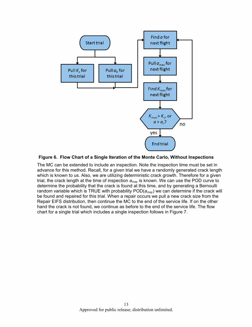
The general method of the MC routine we utilize was suggested by Eric Tuegel. In the absence of inspections, there are three random variables involved: initial crack length a0, fracture toughness Kc, and the maximum applied stress per flight, σmax. a0 and Kc are each constants which are unknown but do not change from flight to flight. σmax is independent from flight to flight and its value changes from flight to flight. Thus in each trial of the MC we need to generate a single value of a0, a single value of Kc, and one value of σmax for each flight in the service life. The routine for a single trial of the MC routine is shown as a flow chart in Figure 6.
13 Approved for public release; distribution unlimited.
Figure 6. Flow Chart of a Single Iteration of the Monte Carlo, Without Inspections
The MC can be extended to include an inspection. Note the inspection time must be set in advance for this method. Recall, for a given trial we have a randomly generated crack length which is known to us. Also, we are utilizing deterministic crack growth. Therefore for a given trial, the crack length at the time of inspection a insp is known. We can use the POD curve to determine the probability that the crack is found at this time, and by generating a Bernoulli random variable which is TRUE with probability POD(a insp) we can determine if the crack will be found and repaired for this trial. When a repair occurs we pull a new crack size from the Repair EIFS distribution, then continue the MC to the end of the service life. If on the other hand the crack is not found, we continue as before to the end of the service life. The flow chart for a single trial which includes a single inspection follows in Figure 7.

14 Approved for public release; distribution unlimited.
Figure 7. Flow Chart of a Single Iteration of the Monte Carlo, Single Inspection
We compare the results of PROF v3.1 and the MC routine through Examples CP4, CP6, and CP7 from the PROF v3 documentation. In addition we run Example CP7 in PROF v2.01. Note that we have adjusted the input parameters from the documentation. Most notably, the crack growth and geometry curves were extrapolated (to a varying degree for each problem) because PROF v3.1 gives a warning when running these problems that the curves should be extended to improve the PROF estimates of SFPOF. The set of inputs to PROF and the MC are shown in full in the Appendix. There were several other minor changes, for example, the number of multiple similar locations per control point was reduced to 1, and the POD parameter Probability Of Inspection (POI) was increased to 1. Important inputs from Example CP7 include: Kc ~ Normal(mean = 83, standard deviation = 4.15), σmax ~ Gumbel(location = 34.229, scale = 0.916), a0 ~ Weibull(shape = 0.575, scale = 0.000219), and ar ~ Weibull(shape = 1.0, scale = 0.0072382).
The MC routine provides a point estimate of SFPOF for any given future flight. Due to the nature of MC simulation this is not a perfect estimate. A confidence interval for the MC estimate can be obtained by performing a bootstrap of the first flight to fail data. This bootstrap confidence interval technique can be applied in either the no inspection or single inspection case. The steps involved are as follows:
• Acquire a sample of size n of the first flight to fail via MC • Create a bootstrap sample of size n by re-sampling the data from Step 1 with
replacement • Calculate SFPOF for the flight of interest using the bootstrap sample obtained in
Step 2 • Repeat Steps 2 and 3 N times, resulting in N bootstrap estimates of SFPOF • The lower and upper bounds of the 95% confidence interval for SFPOF are the 2.5th
and 97.5th quantiles of the N bootstrap estimates of SFPOF, respectively

15 Approved for public release; distribution unlimited.
For Example CP7, we show the results of PROF v2.01, PROF v3.1 and the MC at 1000 flight intervals in Figure 8. The MC was run with sample size n = 10,000,000. Note that for a simple random sampling MC scheme, estimates below 1e-7 are not possible with this sample size (1e-7 corresponds to 1 failure in 10 million trials). The additional point labeled ”MC (IS)” is obtained through an importance sampling procedure discussed below. Also, the MC results utilize the first flight to fail SFPOF equation, not the failure rate version. It does appear that some conservatism was removed from PROF in the update from v2 to v3, but it is clear that, at least for this example from the PROF documentation, roughly two orders of magnitude conservatism remain.
Figure 8. Example CP7 SFPOF Results; No Inspections
The MC results shown in Figure 8 are for the most part above the ASIP recommended threshold of 1e-7, thus is it a legitimate question whether PROF and the MC will yield a similar discrepancy in SFPOF at lower risk levels. As previously stated estimates of SFPOF below 1e-7 are impossible for a simple random sampling scheme including 10 million trials. To obtain accurate estimates for earlier flights, either the number of iterations would need to be increased (which would involve several to many days of run time), or some variance reduction technique could be applied to increase the efficiency of the MC. For the case without inspections, we can run a simple importance sampling scheme in which the EIFS distribution is truncated so that only larger initial cracks will occur (leading to more rapid failure and more data near the SFPOF threshold). One must be careful that the truncation point is selected such that the results at the flight of interest are not biased. This can be accomplished by observing the results of the simple random sampling MC analysis and selecting a crack length below which failure at the early flight of interest is practically impossible.
For Example CP7 PROF hits the 1e-7 threshold at flight number 5,946, thus we wish to select a truncation point below which failure at flight 5,946 would be extremely unlikely. We can plot the first flight to fail against EIFS from the simple random sampling MC routine to help make the decision. This is shown in Figure 9; note the strong dependence of first flight to fail on initial crack length. The truncation point of 0.004" is acceptable because for an EIFS value below this size failure extremely unlikely occur at or before flight 5,946. For the

16 Approved for public release; distribution unlimited.
truncation point of 0.004", the importance sampling scheme is roughly 200x more efficient because the probability of an EIFS value exceeding 0.004" is approximately 0.5% for the EIFS distribution of Example CP7. To account for the truncation of EIFS, the SFPOF estimates obtained from the importance sampling MC run must be multiplied by the probability of observing EIFS larger than the threshold (i.e., the complement of the CDF of EIFS evaluated at the threshold).
Figure 9. Example CP7 MC, First Flight to Fail vs. Initial Crack Length
Bootstrap confidence interval estimates can also obtained when utilizing the importance sampling procedure. As stated, for Example CP7 PROF estimates that the breach of the 1e-7 SFPOF threshold occurs near flight # 5,946. The MC importance sampling estimate for this flight is 9.84e-9 (4.92e-9, 1.57e-8). Also, the MC importance sampling routine suggests that the 1e-7 threshold would be hit around flight 6,750, with 95% CI (8.17e-8, 1.22e-7). If scheduling the first inspection based on the 1e-7 threshold, using PROF would result in an inspection 800 flights early (2.67 years at 300 FH/yr).
A similar plot to Figure 9 for fracture toughness is shown below in Figure 10. The influence of Kc can be seen as a larger value of Kc will likely lead to an increased life, however, EIFS is clearly a more influential variable for this example. We return to the discussion of EIFS and Kc in the next section.
Figure 10. Example CP7 MC, First Flight to Fail vs. Fracture Toughness

17 Approved for public release; distribution unlimited.
The complete results for the no inspection case of Example CP7 are shown in Table 1, in which the results obtained through importance sampling are marked with an asterisk. The SFPOF results for the single inspection results are in Table 2, followed by the PCD results in Table 3.
Table 1. Example CP7; No Inspection, SFPOF Results
Table 2. Example CP7; Single Inspection After Flight 8,000, SFPOF Results
Table 3. Example CP7; Single Inspection After Flight 8,000, PCD Results
The SFPOF results for the no inspection cases of Examples CP4 and CP6 are shown in Figure 11 and Figure 12, respectively. Tabulated results follow in Table 4 and Table 5, respectively. Results for the single inspection cases are omitted as they don’t add to the discussion.
In Example CP4 at the early flights there is an order of magnitude discrepancy between PROF v3.1 and the MC simulation, where the later flights show closer agreement. In Example CP6, there is a consistent discrepancy of between 1 and 2 orders of magnitude. It is interesting to note that there are significant differences between the occurance of two failure modes, K > Kc, and a > ac, in each of the three problems. For CP4, CP6, and CP7, failure due to a > ac occurs in 99.96%, 48%, and ~0%, respectively. Interestingly, CP4 shows best agreement between PROF & MC, CP6 shows roughly one order of magnitude

18 Approved for public release; distribution unlimited.
discrepancy, and CP7 results are two orders of magnitude apart. Thus it appears that PROF v3.1 does a somewhat better job with the undesireable a > ac failure mode, but not with the primary (and preferred) failure mode, K > Kc.
Figure 11. Example CP4 SFPOF Results; No Inspections
Figure 12. Example CP6 SFPOF Results; No Inspections

19 Approved for public release; distribution unlimited.
Table 4. Example CP4; No Inspection, SFPOF Results
Table 5. Example CP6; No Inspection, SFPOF Results
2.6. Improved SFPOF Formulation The PROF formulation of SFPOF has been shown to lead to conservative results. Without considering inspections, one possible reason for PROF’s conservatism is that the PROF SFPOF equation (see PROF documentation) utilizes the crack size distribution f(a) as it would be after having grown EIFS to the time of interest. However, if the initial crack size were large, survival to the flight of interest is relatively less likely. This can be seen by examining a histogram of the EIFS values for the MC trials which survived some number of flights. The histogram of EIFS values for the trials which survived to the 12,000th flight is shown in Figure 13 for Example CP7, along with the original EIFS curve in red. Clearly those trials for which the initial crack size was larger than 0.001” have little to no chance of survival to the 12,000th flight, thus when we are calculating the probability that flight 12,000 is the first flight to fail we should incorporate the very strong evidence that the initial crack size must have been relatively small. The crack size distribution at flight 12,000 is in actuality the result of growing this histogram for 12,000 flights, not the result of growing EIFS for 12,000 flights. If the crack size distribution resulting from growth of the original EIFS distribution is used to estimate SFPOF for the 12,000th flight, the result will be an overestimate.

20 Approved for public release; distribution unlimited.
Figure 13. Example CP7 MC, Initial Crack Length For Trials Surviving 12,000 Flights A similar plot can be generated for Kc. However, because the influence of Kc on survival is not as strong as that of EIFS, to see a difference between the initial distribution of Kc and the distribution of Kc for only those iterations which survived to a later flight, one needs to examine a later flight. The histogram of Kc for trials which survived 14,750 flights is shown in Figure 14, along with the curve of the original PDF of Kc in red. Note that survival indicates that the initial crack size was likely smaller, and that the fracture toughness is likely higher.
Figure 14. Example CP7 MC, Fracture Toughness For Trials Surviving 14,750 Flights The histograms in Figure 13 and Figure 14 are obtained through the MC procedure, thus requiring a significant amount of run time to acquire. SFPOF for any flight can be accurately calculated if one knows the distributions of crack length and fracture toughness at that time. If we can reliably and accurately find these survival-incorporated distributions analytically,

21 Approved for public release; distribution unlimited.
we could obtain accurate estimates of SFPOF without needing to run the expensive MC routine. We show in this section that it is possible to use Bayes’ rule to simultaneously update the distributions for EIFS and Kc given survival to the flight of interest, and that once these distributions are obtained they can be used to accurately calculate SFPOF. First we demonstrate that simultaneous updating of multiple variables can be accomplished with Bayes’ rule through a much simplified example.
Suppose that EIFS is a random variable A with only two possible states: a1 (small) and a2 (large). Similarly, fracture toughness is a random variable K (the subscript c is dropped for this discussion to simplify the notation; please do not confuse K with stress intensity) with two states: k1 (low) and k2 (high). We have in effect discretized the distributions of both A and K to two states each. The third random variable is that of survival, S, with states T (true) and F (false). Our goal is to obtain the joint distribution of A and K given survival (S=T). We utilize the following version of Bayes’ formula.
Pr(𝐴,𝐾|𝑆 = 𝑇) =Pr(𝐴,𝐾, 𝑆 = 𝑇)
Pr(𝑆 = 𝑇)=
Pr(𝑆 = 𝑇|𝐴,𝐾)Pr(𝐴,𝐾)Pr(𝑆 = 𝑇)
Assume for the time being that the probability of survival to the flight of interest can be calculated if the states of A and K are known; this is Pr(𝑆 = 𝑇|𝐴,𝐾). In our actual example we describe how this is found. We arbitrarily specify the relevant distributions as follows. In Bayesian terminology Pr(𝐴) and Pr(𝐾) are the prior distributions for A and K, respectively.
Pr(𝐴) = �Pr(𝑎1)Pr(𝑎2)� = �0.6
0.4�
Pr(𝐾) = �Pr(𝑘1)Pr(𝑘2)� = �0.3
0.7�
Pr(𝑆 = 𝑇|𝐴,𝐾) = �Pr(𝑆 = 𝑇|𝑎1, 𝑘1) Pr(𝑆 = 𝑇|𝑎1, 𝑘2)Pr(𝑆 = 𝑇|𝑎2, 𝑘1) Pr(𝑆 = 𝑇|𝑎2, 𝑘2)� = �0.7 0.9
0.6 0.8�
Note that the distribution of Pr(𝑆 = 𝑇|𝐴,𝐾) has a been defined such that the probability of survival is highest when the initial crack size is small and the fracture toughness is large, and lowest when the reverse is true; this is consistent with the realistic situation. The joint distribution of A and K can be easily determined because these variables are independent. For example, Pr(𝑎1, 𝑘1) = Pr(𝑎1)Pr(𝑘1) = 0.6 ∗ 0.7 = 0.42. The joint distribution can be conveniently obtained through matrix multiplication as follows.
Pr(𝐴,𝐾) = 𝐴𝐾′ = �Pr(𝑎1)Pr(𝑎2)� [Pr(𝑘1) Pr(𝑘2)] = �0.6
0.4�[0.3 0.7] = �0.18 0.42
0.12 0.28�
Lastly, we require the probability of survival, Pr(𝑆 = 𝑇). This is calculated as follows.
Pr(𝑆 = 𝑇) = � � Pr(𝑎𝑖 ,𝑘𝑗)Pr�𝑆 = 𝑇�𝑎𝑖 ,𝑘𝑗�𝑗=1,2𝑖=1,2
= 0.18 ∗ 0.7 + 0.12 ∗ 0.6 + 0.42 ∗ 0.9 + 0.28 ∗ 0.8
= 0.8
22 Approved for public release; distribution unlimited.
Bayes’ rule can now be applied one cell at a time as follows.
Pr(𝑎𝑖 ,𝑘𝑖|𝑆 = 𝑇) =Pr(𝑆 = 𝑇|𝑎𝑖 , 𝑘𝑖)Pr(𝑎𝑖 ,𝑘𝑖)
Pr(𝑆 = 𝑇)
The overall result is as follows. In Bayesian terminology this is referred to as the posterior joint distribution of A and K, where Pr(𝐴,𝐾) is the prior joint distribution.
Pr(𝐴,𝐾|𝑆 = 𝑇) = �0.1575 0.47250.0900 0.2800�
The marginal posterior distributions of A and K are found by summing across the columns and rows of Pr(𝐴,𝐾|𝑆 = 𝑇), respectively. These are: Pr(𝐴|𝑆 = 𝑇) = �0.63
0.37� and Pr(𝐾|𝑆 =
𝑇) = �0.24750.7525�. Survival indicates that relative to the prior distributions of A and K the smaller
initial crack size and the larger fracture toughness are more likely the truth, as expected. It is more correct to calculate SFPOF using the updated distributions of A and K.
In the simple example just shown we discretized the naturally continuous distributions of EIFS and fracture toughness to two possible states for each random variable. Such coarse discretization is clearly not adequate to accurately represent these random variables. We can discretize to a large number of states and perform the identical calculation above to estimate SFPOF for Example CP7 using Bayes’ rule. Note that any continuous distribution can be approximated with a discrete distribution, with perfect representation as the number of states 𝑛 → ∞.
Note that in the simple example we did not show how to calculate the probability of survival of either a flight or an interval of flights as a function of the crack size and the fracture toughness. We need this capability to calculate SFPOF for Example CP7 using Bayes’ rule. Note that from this point forward K denotes stress intensity and Kc denotes fracture toughness. The following assumptions are sufficient for this discussion.
• EIFS, fracture toughness, and maximum applied stress per flight are mutually independent random variables
• Maximum applied stress per flight is Gumbel distributed and independent from flight to flight
• Crack growth is a deterministic function of time elapsed • The normalized stress intensity K/σ is a determinstic function of crack length • The maximum stress intensity encountered during a flight, Kmax, is a function of crack
length and the maximum applied stress for that flight
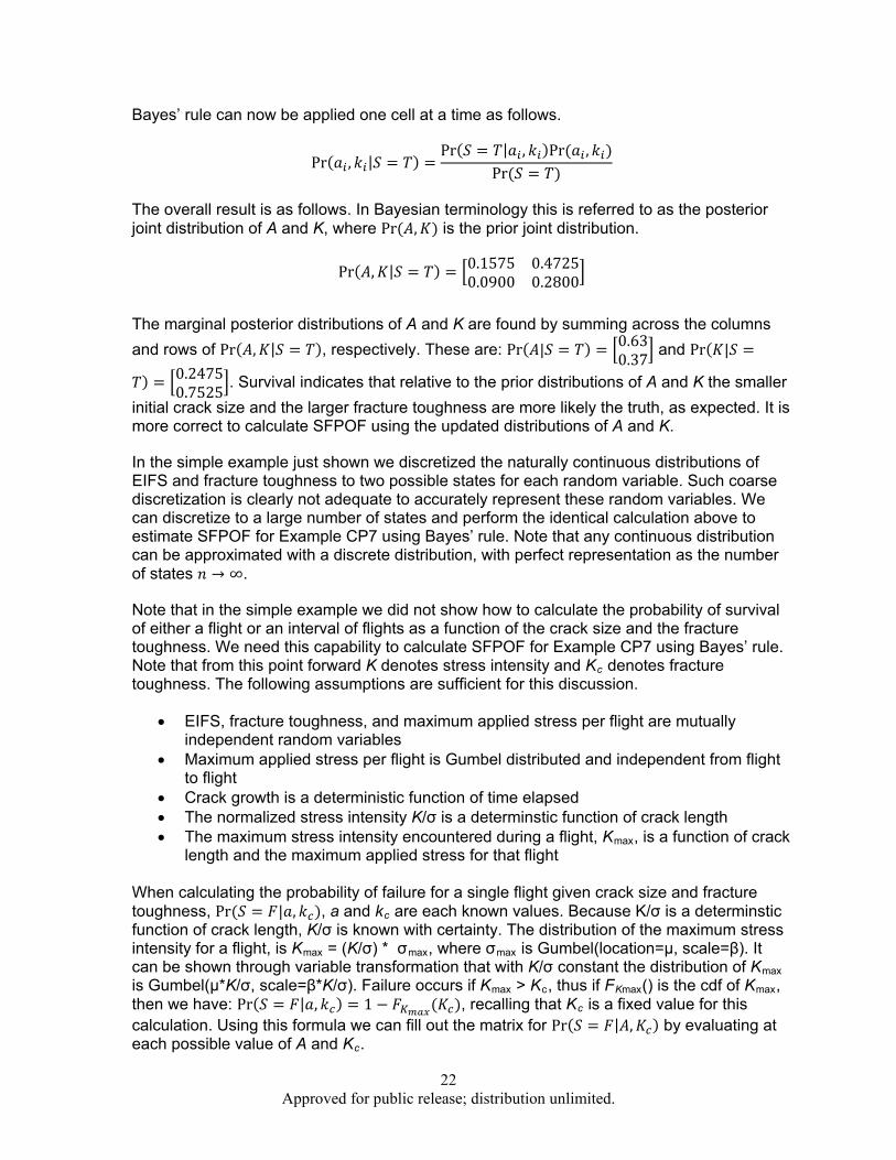
When calculating the probability of failure for a single flight given crack size and fracture toughness, Pr (𝑆 = 𝐹|𝑎, 𝑘𝑐), a and kc are each known values. Because K/σ is a determinstic function of crack length, K/σ is known with certainty. The distribution of the maximum stress intensity for a flight, is Kmax = (K/σ) * σmax, where σmax is Gumbel(location=μ, scale=β). It can be shown through variable transformation that with K/σ constant the distribution of Kmax is Gumbel(μ*K/σ, scale=β*K/σ). Failure occurs if Kmax > Kc, thus if FKmax() is the cdf of Kmax, then we have: Pr(𝑆 = 𝐹|𝑎, 𝑘𝑐) = 1 − 𝐹𝐾𝑚𝑎𝑥(𝐾𝑐), recalling that Kc is a fixed value for this calculation. Using this formula we can fill out the matrix for Pr(𝑆 = 𝐹|𝐴,𝐾𝑐) by evaluating at each possible value of A and Kc.

23 Approved for public release; distribution unlimited.
For example, suppose a = 0.4089” and Kc = 80 ksi*in1/2. Consulting the normalized stress intensity table for Example CP7 in Table A.2, K/σ = 1.4557. For Example CP7, σmax ~ Gumbel(μ = 34.229, β = 0.916). We have Kmax ~ Gumbel(μ*K/σ = 49.827, β*K/σ = 1.333). The complement of the CDF of Kmax evaluated at Kc is the probability of failure for this flight: 1 − 𝐹𝐾𝑚𝑎𝑥
(80) = 1.488𝑒−10. This calculation must be performed for all combinations of a and kc to generate a matrix Pr(𝑆 = 𝐹|𝐴,𝐾).
Note that we have implicitly assumed that the amount of crack growth over the course of a flight is neglible because we have represented the crack length for a flight as a constant. For a 1.3 hour flight, this assumption can be shown to have almost no effect on SFPOF results. If a much longer flight were being considered (such as for a reconnoisance drone) this assumption would require evaluation. Similarly we have represented a range of Kc (generally a short interval) by a single value. The discretization must be sufficiently fine such that the discretization error introduced is acceptably low.
We have obtained a means for calculating the probability of failure for an individual flight. For a sequence of flights, given the independence assumptions above, the probabilities of failure for each flight in a sequence are independent. Also, because crack growth is a deterministic function, the crack size, and consequentially K/σ, are known with certainty for each flight in the sequence. Thus we can find the probability of failure for each flight in a sequence with Pr(𝑆 = 𝐹|𝑎, 𝑘𝑐) = 1 − 𝐹𝐾𝑚𝑎𝑥(𝐾𝑐), where a is the crack size at the start of the sequence. If pi is the probability of failure for the ith flight in the sequence (calculated in the manner described above), and the pis are independent, then the probability of surviving n flights is ∏ (1 − 𝑝𝑖)𝑛
𝑖=1 .
Calculation of SFPOF for Example CP7 using Bayes’ rule can now proceed. The EIFS distribution is discretized to 1000 states using log scaling so that the small crack sizes are well represented (the log spacing is evident in Figure 15 as the bins are more tightly spaced at the lower end of crack sizes). Kc is discretized to 200 states using standard spacing out to 8 standard deviations from the mean. Discretization involves first partitioning the support of the distribution into a number of intervals, then evalutating the CDF of the continuous distribution at the lower and upper bounds of each interval to determine the probability mass located in each bin of the partition. This problem is identical to the simple two state example shown above; the only complication is that there are far more than two states to represent EIFS and Kc.
Consider the plot below in Figure 15, which is related to Figure 13. In the earlier figure a histogram of the EIFS values which survived 12,000 flights in the MC routine was shown in which the histogram was composed of several dozen crack size bins. We show a similar histogram below which bins over the same intervals used to discretize EIFS, and we overlay the prior distribution of EIFS as well as the distribution of Pr(𝐴|𝑆 = 𝑇) obtained by updating EIFS for Example CP7 using Bayes’ rule to reflect survival for 12,000 flights. Bayes’ rule matches the MC result very well, thus we are confident that the application of Bayes’ rule is behaving. A similar plot for Kc is shown in Figure 16, as before extending the interval to 14,750 flights so that the shift in the distribution is visible.

24 Approved for public release; distribution unlimited.
Figure 15. Example CP7 MC, EIFS Updated With Bayes Rule, Surviving 12,000 Flights
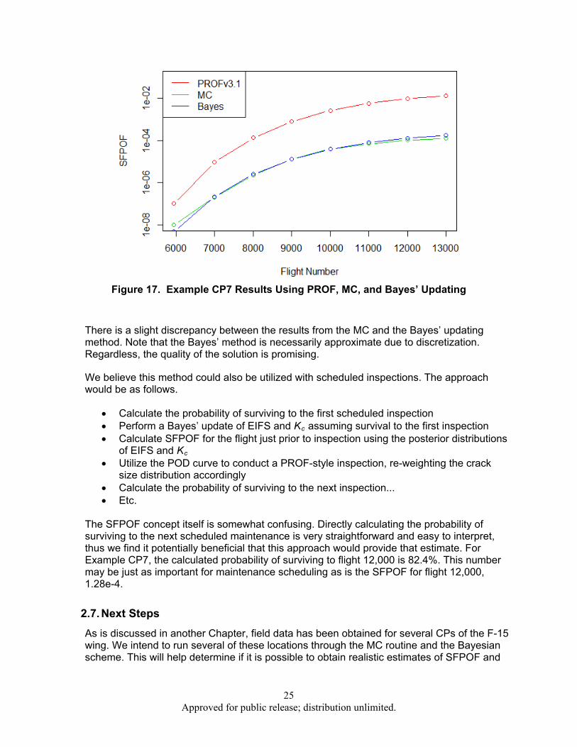
Figure 16. Example CP7 MC, Kc Updated With Bayes Rule; Surviving 14,750 Flights We perform the calculation of SFPOF for Example CP7 for the same flights as Figure 8. Note that after updating for survival, the posterior EIFS distribution needs to be ”grown” for the appropriate number of flight hours to obtain the discretized crack size distribution for the flight of interest. We then use that distribution, along with the posterior distribution of Kc, to calculate SFPOF for a single flight. The results for Example CP7 from PROF v3.1, the MC routine with 10,000,000 iterations (importance sampling used for the first MC flight calculated), and the Bayes’ updating approach are shown in Figure 17. Note the Bayes’ solution is obtained in a matter of moments, where the MC solution required >10 hours of runtime.
25 Approved for public release; distribution unlimited.
Figure 17. Example CP7 Results Using PROF, MC, and Bayes’ Updating
There is a slight discrepancy between the results from the MC and the Bayes’ updating method. Note that the Bayes’ method is necessarily approximate due to discretization. Regardless, the quality of the solution is promising.
We believe this method could also be utilized with scheduled inspections. The approach would be as follows.
• Calculate the probability of surviving to the first scheduled inspection • Perform a Bayes’ update of EIFS and Kc assuming survival to the first inspection • Calculate SFPOF for the flight just prior to inspection using the posterior distributions
of EIFS and Kc • Utilize the POD curve to conduct a PROF-style inspection, re-weighting the crack
size distribution accordingly • Calculate the probability of surviving to the next inspection... • Etc.
The SFPOF concept itself is somewhat confusing. Directly calculating the probability of surviving to the next scheduled maintenance is very straightforward and easy to interpret, thus we find it potentially beneficial that this approach would provide that estimate. For Example CP7, the calculated probability of surviving to flight 12,000 is 82.4%. This number may be just as important for maintenance scheduling as is the SFPOF for flight 12,000, 1.28e-4.
2.7. Next Steps As is discussed in another Chapter, field data has been obtained for several CPs of the F-15 wing. We intend to run several of these locations through the MC routine and the Bayesian scheme. This will help determine if it is possible to obtain realistic estimates of SFPOF and

26 Approved for public release; distribution unlimited.
PCD under the assumptions that a crack exists at time zero and that crack growth is deterministic.
In the event that the estimates obtained do not match our intuition about the actual risk of the structure, which we suspect will be the case, we will proceed to examine the possibility of relaxing the above assumptions. The MC scheme presented in this chapter is immediately applicable for this purpose. When growing the cracks from flight to flight within a trial, stochastic crack growth can be used. Similarly, at the beginning of a trial (or after a repair) an initiation period can occur in which the crack has not yet begun to grow. This can be used to obtain realistic estimates of SFPOF and PCD, or to validate other methods which incorporate stochastic crack growth and crack initiation in the analysis.
In addition, we will continue to develop the MC routine. A Fortran version is currently in work that will, barring unforeseen difficulties, incorporate the use of multiple processors/cores to increase the speed of the computation.

27 Approved for public release; distribution unlimited.
3. System Risk Analysis
3.1. Introduction
It is well known that the failure events for structural locations are highly correlated. This allows one to focus design, analysis and testing on a few critical components. However, as more novel structures are developed, aircraft are produced with limited production runs, and aircraft operate in extreme environments, it is likely that prior knowledge of critical locations based on experience will be lacking, and that traditional deterministic criteria will be insufficient. Hence, there is a need to research and develop more robust probabilistic-based methods that can determine critical locations considering random variable inputs and correlation between failure locations. This section describes the application of an AFRL-funded system reliability methodology [24] to SFPOF calculations. The methodology is called Reliability-based Filtering Method (RFM) in that non-critical locations are filtered based on a reliability-based relative error indicator. The application to Single Flight Probability of Failure calculations is a new application of RFM to aircraft structures. Preliminary results from this application are documented below.
3.2. Methodology
The limit state, g(x) , is defined in terms of the failure model such that g 0 denotes failure and x represents a vector of random variables. g(x) represents any quantify of interest at any location or time step in the analysis, e.g., displacement at a node, applied stress less than residual strength, etc. An ideal system-reliability-based metric would be to determine the relative change in the system reliability should an individual limit state be filtered, e.g.,
ˆ i
P g j (x) 0j1
m
U
P g j (x) 0
j1j i
m
U
P g j (x) 0j1
m
U
(1)
then compare ˆ i against an error tolerance, Tol . If the ˆ i< Tol , the limit state is filtered. However, this approach is not practical since calculating the system reliability of a large number of limit states is unfeasible. As a surrogate, a pair-wise filtering method is proposed. Application to date shows that this method is quite effective in determining the critical limit states. The pair-wise comparison equation is shown in Eq. (2)
i
P[g1 giU ] P[g1]
P[g1] i 2,n (2)
In this case, the relative error incurred by filtering limit state gi relative to another limit state g1 is computed. g1 denotes a comparison limit state, which is the limit state with the highest POF.
P[g1 giU ] is the probability of failure encompassed by both g1 and gi . Once i is computed, the decision to keep or filter a limit state is based upon a comparison of the relative error, i , against an error tolerance, Tol ; the decision process is shown in Eq. (3),
i Tol filter limit state
i Tol keep limit state (3)

28 Approved for public release; distribution unlimited.
where
γTol is the filtering error tolerance that can be set according to the preferences of the user. In other words, if
γ i < γTol , the relative error in the POF incurred by filtering limit state
gi relative to the joint POF considering both
g1 and,
gi is less than
γTol and the corresponding
gi can be filtered. The concept of pair-wise filtering is shown in Figure 18. The base of the graph shows 2 limit states (black and red for Figure 18(a), and black and blue for Figure 18(b). The colored region (red in a, blue in b) shows the region that will be ignored if the red or blue limit state is filtered. The top of the graph shows the joint PDF that will be integrated to compute the probability. It is clear from the graphs that there is a large relative error for
γ i as shown in Figure 18(a) (
γ i=0.3) and a much smaller relative error for Figure 18(b) (
γ i=0.006).
Figure 18. Examples of pair-wise filtering
a) large error if red limit state is filtered, b) small error if blue limit state is filtered
3.2.1. Subsequent Filtering
Once the initial filtering has been carried out, a pool of limit states exist each of which has an error indicator greater than
γTol relative to
g1. However, some of the limit states within the pool may filter out other limit states within the pool. Therefore, the filtering method is repeated recursively using only the limit states remaining within the pool. For example, the limit state within the pool with the largest POF is designated as the new
g1, then the error indicators are computed for all remaining limit states in the pool, then each limit state is filtered or not based on Eq. (3). This is shown graphically in Figure 19. Here, the blue limit state clearly filters the purple limit state and the green limit state filters the red limit state. The end result of this process is another pool for which the filtering is again invoked. This process is repeated recursively until all pools have been processed.

29 Approved for public release; distribution unlimited.
Figure 19. Example of subsequent filtering
3.2.2. Calculation Methods
A critical element of this method is accurate calculation of the joint probability P[g1 giU ]. This
probability must be accurately computed for any correlation coefficient, particularly values near 1, e.g., 0.999. In practice, one finds that the structure causes a high level of correlation between limit states. In addition, the evaluation must be efficient since the method must scale for a large number of limit states. The evaluation of the joint POF can be facilitated through the transformation of the integral to standard normal space. This transformation is a natural approach used in the First Order Reliability Method (FORM).
ui 1[Fxi (xi)] i 1,2,K ,n (4)
Once the integral has been transformed to standard normal space, P[g1 giU ] can be computed
as
P[g1 giU ] 12(1,i,1i) (5)
where 2(1,i,1i) denotes the bivariate standard normal integral, 1 1(P[g1 0])
denotes the safety index for g1, i denotes the safety index for gi , and 1i is the correlation
coefficient between limit states g1 and gi . It should be noted that the integral P[g1 giU ] is n
dimensional, where n denotes the number of random variables, whereas the right hand side is a 2 dimensional integral. Clearly, this is a very large savings in computational complexity. Also, implicit in Eq. (5) is the fact that the correlation coefficient 1i on the left hand side represents the correlation between the limit states whereas 1i on the right hand side represents the correlation between random variables. This concept of the transformation of the meaning of the correlation coefficient is demonstrated in Figure 20 below.

30 Approved for public release; distribution unlimited.
Figure 20.
Φ2 calculation mapping the correlation from limit states to random variables
Evaluation of
Φ2 integral The calculation of the bivariate standard normal integral has been well studied. However, for our implementation, an efficient, highly accurate result is needed, particularly for high correlation. Tong [19] presents a 1 dimensional integral for
Φn (n dimensional standard normal integral) valid for n limit states with constant correlation coefficients and all correlation coefficients
≥ 0 ,
Φn (β;ρ) = φ(t) Φβi − ρt
1− ρ
i=1
n
∏−∞
∞
∫ dt (6)
where
φ and Φ are the one dimensional standard normal PDF and CDF, respectively. For two limit states, Eq. (6) reduces to
Φ2(β;ρ) = φ(t)Φ β1 − ρt1− ρ
Φ
β i − ρt1− ρ
−∞
∞
∫ dt (7)
Solution of this integral using Gauss-Hermite quadrature shows good accuracy with reasonable computational effort. However, the effort increases significantly as
ρ →1. The best method known to integrate
Φ2 is the formulation by Drezner and Wesolowski [20] as modified by Genz [21]. This algorithm has been tested and reproduces the author’s claim that the maximum error is 5E-16 for all correlation coefficients using at most 20 integrand evaluations.
3.3. Cumulative Effects The pair-wise filtering algorithm is effective at examining 2 limit states at a time. Once the filtering is complete, the cumulative effect of all the filtered limit states can be evaluated using 2nd order bounds [22]. If the difference in bounds between two cases a) using only the remaining unfiltered limit states, and b) using all limit states is significant, then
γTol should be lowered to keep more limit states and the process repeated.

31 Approved for public release; distribution unlimited.
3.4. Filtering Application The basic RFM approach has been implemented in a simple application that can be used once either the FORM approximation or the correlations between the limit states has been determined. The application has a simple interface which is illustrated in Figure 21.
Figure 21. Interface to Filtering Application
The application allows for either the FORM approximation alphas or the correlations to be used as input to the process.
3.5. FORM Approximation As indicated in the previous discussion, one of the filtering approaches utilizes the information from a FORM approximation to the various limit states. The FORM approximation involves identifying the Most Probable Point (MPP) in standard normal space. This is the location of the point on the linear approximation to the limit state function that is closest to the origin. The magnitude of the distance to the origin is the value of beta, and the cosines of the angles from the coordinate axes are the values of the alphas that are required for the filtering process. Finding the MPP in the case of no inspections is fairly straight forward, however, the process becomes more challenging when inspections occur and repairs are made. The process of finding the MPP involves transforming the state variables to standard normal space and then using a constrained optimization process to find the MPP. The constraint in this process is simply the limit state function that the variables must satisfy. For the case of no inspections, the

32 Approved for public release; distribution unlimited.
process of transforming the variables to standard normal space is well defined and straight forward. The inverse CDF function for each random variable is required in the transformation process and this is where the inspection process complicates things. At an inspection some cracks will be discovered and repaired so that the CDF of the crack size will become a combination of the distribution of cracks before inspection and the distribution of cracks that were repaired as a result of the inspection. This distribution cannot be expressed in a simple functional form but has to be developed therefore in a digitized, or tabular, fashion. As indicated, the density of crack sizes after inspection will be the sum of the percent of cracks detected (Pdet) times the density of repair crack sizes and the percent of cracks not detected times the density of cracks before inspection
(8) where
(9) Since the inverse CDF is required, the expression for the density must be integrated, thus:
(10) Having this result, an inverse CDF table can be created to provide the needed transformation:
(11) This result can then be used by the FORM approximation process to provide the necessary transformation between real space and standard normal space. The steps in this process are relatively straight forward; however, the challenges lie in the implementation details. This is particularly true for the process of getting the density of cracks just before inspection. This is done using the EIFS distribution of flaws and analytically growing them out to the time that the inspection occurs. Typically the crack growth behavior is given in a tabular manner which must have sufficient resolution, particularly in the small crack range, so that the EIFS distribution can be grown to a meaningful distribution at inspection time. The EIFS distribution is typically much smaller than the crack sizes used to define the crack growth curve, so this presents some significant challenges. Finding a constrained optimization routine that would be useful in computing the MPP was a bit of a challenge. The optimization package ADS (Automated Design Synthesis) that was developed under NASA contract by Garrett Vanderplaats was chosen [23]. This package exists as a large FORTRAN subroutine which was compiled into a static library. An interface layer

33 Approved for public release; distribution unlimited.
between the Java user interface and the static library was developed in C++ and is compiled into a dynamic linked library (dll). This dll is used in building the Java application and allows the Java code to execute a call to the ADS routine and pass the parameters that it requires. The basic structure of the application is quite simple and this is a result of the architecture of the ADS routine and the way it handles the optimization process. The structure is illustrated in Figure 22.
Figure 22. Structure of Constrained Optimization Process
The ADS source code is in the public domain and will be available along with all the other code for these applications. The user interfaces have been kept as simple as possible while still providing the ability for the user to easily input all information required by the code. This was done to avoid an excessive amount of effort on the polish of the interface rather than on developing a solid analytical framework for the methods. User convenience and other features can always be added at a later date if there are some enhancements that are desirable.
3.6. Current Progress The FORM approximation application has been developed and is currently in a validation stage. The basic user interface is shown in Figure 23.

34 Approved for public release; distribution unlimited.
Figure 23. User Interface for FORM Approximation Application
The application is currently set up to handle only one inspection event, but could be extended to allow multiple inspections. The input file contains the same information that would go into PROF or RBDMS codes. This input currently contains the file names of the crack growth curve and the beta curve, both of which can be obtained from an analysis package such as Boeing’s Lifeworks. The statistical distributions available for the various parameters are currently constrained by the same requirements imposed by the PROF code. Once a particular control point has been analyzed, the application offers an ability to store the result in a file for use in the filtering application. The filtering application takes the information from a number of limit states (in this case control points) and determines which are the most significant in terms of the overall reliability of the total system. With that in mind, the analysis of a particular control point can be appended to an existing file so that the user can easily build up an input file for the filtering application without any manual intervention.
3.7. Future Efforts
3.7.1. FORM Approximation Tool
The FORM approximation tool is currently being validated and the issues relating to the tabular form of the crack growth curve mentioned previously are being addressed. To date, the non-inspection results have compared exceedingly well with the results obtained by Dr. Millwater in

35 Approved for public release; distribution unlimited.
his development environment. The results obtained with inspections compares well also when analytical distributions are used and solutions to the tabular lookup process are being considered.
3.7.2. Correlations from Sampling
The filtering process can also be conducted directly with the correlations between the limit states (control points). As an alternative to the FORM approximation, the direct calculation of the correlations using sampling methods is being developed. This will provide an alternate method to provide the filtering application with the information it requires.
3.7.3. System Risk Calculation
A final step in the process will be the calculation of the overall system risk once the reduced set of limit states has been determined. The user will then have a three step process, first determine either the correlations or FORM approximations for all limit states, then perform the filtering, and last calculate the total system reliability.
3.7.4. F-15 Control Points
The F-15 control point data will be used to demonstrate the benefits of the filtering process. This will proceed in a series of steps designed to demonstrate some of the behaviors of the filtering and system risk as the service life of the fleet progresses. First, as a baseline, the filtering process will be run assuming no correlation between the control points and no inspections. Subsequently the filtering application will be run with the correlation, or FORM approximation, information to show the beneficial effects of the filtering in reducing the number of control points that need to be considered. Second, the correlations or FORM approximations will be done after an inspection event along with the subsequent filtering. This will potentially illustrate that the most significant control points are changed after inspections due to some points being identified and repaired. It’s clear that the importance of the various control points will evolve over time as the aircraft ages due to the inspection and repair process as well as to the difference in the crack growth behavior at the different locations.

36 Approved for public release; distribution unlimited.
4. Cost Analysis
4.1. Update to the models
The Cost/Benefit Analysis (CBA) contains a set of three Microsoft Excel workbooks, and each represents the various system configurations under evaluation. There is a workbook for the Baseline configuration, another for the Optimized Non Destructive Evaluation (Opt NDE) configuration, and a final version for the Optimized Structural Health Monitoring (Opt SHM) configuration. All three workbooks are structurally identical, with the exception of a Return on Investment (ROI) calculator included in the Opt SHM version. This extra functionality allows the Opt SHM workbook to calculate the time to recoup an investment in either the Opt NDE or Opt SHM configuration when compared to the Baseline. The ROI calculator performs these calculations by importing the lifecycle cost from the other two workbooks and then uses that data to determine how many years it takes before the incurred expense of an SHM system is more cost effective than that of the other two configurations. It also determines the time to recoup an investment in the NDE configuration versus the Baseline.
Since the last progress report a minor update was made to the workbooks. The
initial results of the Financial Uncertainty Analysis (FUA) exposed a need for a simple formula to be added to the “CP Info” tab of the workbook. This was due to an inability to validate the model’s calculations because we could not take a set of randomly generated inputs from the uncertainty model and manually recreate that model run’s outputs in the workbooks. It was determined that the error was an earlier version of the FUA model independently varied both the Part Replacement Cost (PRC) and the Inflight Failure Cost (IFFC) when in actuality the IFFC is either the total platform cost or the PRC. In other words, the PRC and IFFC should not have both been independently varied. To remove this error, each cell for IFFC on the “CP Info” is now either a simple formula that pulls over the PRC from the column next to it, or it is a user input of the total platform replacement cost. The decision to select PRC or total platform cost is based on previously conducted risk analysis that determines whether damage to a specific CP is repairable or will cause a total loss of the airplane. To reflect this change in the FUA model the IFFC was removed as a varied input since it is now either a static input or a formula.
To illustrate the updates from the above section, Figure 24 shows the high level
picture of the “CP Info” tab’s format from the CBA workbooks previously provided along with the User Manual. In accordance with the manual, yellow cells are those requiring a user input value.

37 Approved for public release; distribution unlimited.
Figure 24. Previous version of the CBA workbook’s “CP Info” tab
Figure 25 shows the new, updated version of the workbook where the IFFC column has both yellow cells indicating a user input or green cells indicating a need for a minor user-designated formula. All of the orange cells are inputs to the FUA.
Figure 25. Revised version of the CBA workbook’s “CP Info” tab
For clarity, Figure 26 is a zoomed in picture of the top four rows of the revised
workbook along with the column headers shown in Figure 25.
Figure 26. Zoomed in picture of the revised workbook

38 Approved for public release; distribution unlimited.
With the repair of the error discussed above, the structure of the Financial Uncertainty Analysis (FUA) model is complete. The model takes approximately 6.5 hours to complete 5000 runs, and we generated a run of 15,000. Figure 27 shows the general structure of the model.
Figure 27. Structure of the Financial Uncertainty Analysis Model
The structure of the model shows how the Baseline configuration is used by both
the Opt NDE and Opt SHM configurations in order to compare the total cost of the systems with respect to the Baseline. The model also automatically pulls the Baseline and Opt NDE information needed for the Opt SHM workbook to perform the Return on Investment calculations. A Monte Carlo probabilistic analysis tool is then used to select a set of randomly generated inputs for each run of the model and consistently applies them to all three workbooks. It then captures the resulting outputs in order for statistical analysis to be conducted on them.
There are 225 inputs to the uncertainty model that vary general cost of
performing maintenance activities but also the cost of purchasing then supporting an SHM system. The selection of the inputs induces variations in all three of the configurations, including the baseline. The workbooks’ “CP Info” data for each of the Control Points makes up the largest portion of the inputs, and each CP’s boundary values are shown below in Table 6. Each of the values has a nominal value determined by a Subject Matter Expert, and then centered on that value the model applies a lognormal distribution with a 10% standard deviation within the specified boundaries. The lognormal distribution and standard deviation was selected in order to reflect that an established maintenance program has well defined timelines to conduct maintenance activities. However, it is necessary to include the human element in the uncertainty calculations, so a lognormal distribution allows us to show that some people might take longer to conduct the task while learning the process but then have a positive learning curve leading to most of their tasks over time being conducted according to the expected hours. The lognormal distribution when applied over the platform’s service life also allows us to reflect the transient, rotational nature of the military workforce. Even in the case of experienced mechanics, when they move from one permanent duty station to another there is a loss of corporate knowledge and a consequent learning curve for their replacement.

39 Approved for public release; distribution unlimited.
Table 6. Control Point data varied in the FUA model
The rest of the inputs to the model are included below in Table 7. These items
are more general to the costs of the performing the airplane’s maintenance as well as the cost to purchase and then maintain the SHM sensor suite. These inputs all have a nominal value used in the CBA to evaluate an actual system of record, and for the uncertainty analysis they are varied uniformly within the specified limits.
CP NDE Time SCRT MCRT LCRT IFFC PRCMed Low Hi Med Low Hi Med Low Hi Med Low Hi Med Low Hi Med Low Hi
054B 3 2.7 6 8 7.2 16 0 - - 80 72 100 5000 4500 10000 5000 4500 10000054C 3 2.7 6 8 7.2 16 0 - - 80 72 100 5000 4500 10000 5000 4500 10000055 2 1.8 4 8 7.2 16 60 54 75 160 144 184 29900000 50000 45000 60000056 3 2.7 6 12 10.8 24 84 75.6 105 160 144 184 29900000 60000 54000 72000
057B 2 1.8 4 8 7.2 16 84 75.6 105 160 144 184 29900000 60000 54000 72000059B 7 6.3 14 12 10.8 24 84 75.6 105 160 144 184 29900000 60000 54000 72000063B 3 2.7 6 12 10.8 24 72 64.8 90 80 72 100 5000 4500 10000 5000 4500 10000097 2 1.8 4 12 10.8 24 0 - - 200 180 230 29900000 100000 90000 120000
112B 3 2.7 6 12 10.8 24 64 57.6 80 120 108 138 25000 22500 32500 25000 22500 325000114 3 2.7 6 32 28.8 48 64 57.6 80 80 72 100 10000 9000 15000 10000 9000 15000115 2 1.8 4 8 7.2 16 32 28.8 48 72 64.8 90 5000 4500 10000 5000 4500 10000116 2.5 2.25 5 8 7.2 16 32 28.8 48 72 64.8 90 5000 4500 10000 5000 4500 10000
124B 3 2.7 6 8 7.2 16 60 54 75 160 144 184 29900000 50000 45000 60000126B 2 1.8 4 8 7.2 16 32 28.8 48 100 90 125 29900000 15000 13500 22500130B 3 2.7 6 32 28.8 48 64 57.6 80 80 72 100 10000 9000 15000 10000 9000 15000131 2.5 2.25 5 12 10.8 24 72 64.8 90 80 72 100 5000 4500 10000 5000 4500 10000
133A 1 0.9 2 6 5.4 12 0 - - 16 14.4 32 500 450 1000 500 450 1000134B 2.5 2.25 5 8 7.2 16 40 36 50 120 108 138 40000 36000 48000 40000 36000 48000135B 2 1.8 4 8 7.2 16 16 14.4 32 80 72 100 25000 22500 32500 25000 22500 32500137B 2 1.8 4 8 7.2 16 16 14.4 32 80 72 100 25000 22500 32500 25000 22500 32500138B 2 1.8 4 8 7.2 16 40 36 50 120 108 138 40000 36000 48000 40000 36000 48000139 2 1.8 4 8 7.2 16 32 28.8 48 72 64.8 90 5000 4500 10000 5000 4500 10000140 2 1.8 4 8 7.2 16 32 28.8 48 72 64.8 90 5000 4500 10000 5000 4500 10000141 2 1.8 4 8 7.2 16 32 28.8 48 72 64.8 90 5000 4500 10000 5000 4500 10000143 2 1.8 4 4 3.6 8 32 28.8 48 160 144 184 20000 18000 26000 20000 18000 26000144 2 1.8 4 24 21.6 36 40 36 50 60 54 75 5000 4500 10000 5000 4500 10000145 3.5 3.15 7 8 7.2 16 24 21.6 36 80 72 100 2500 2250 5000 2500 2250 5000
166B 3 2.7 6 24 21.6 36 60 54 75 240 216 276 29900000 100000 90000 120000179 2.5 2.25 5 8 7.2 16 32 28.8 48 160 144 184 29900000 60000 54000 72000180 2.5 2.25 5 8 7.2 16 32 28.8 48 160 144 184 29900000 60000 54000 72000181 2 1.8 4 8 7.2 16 32 28.8 48 100 90 125 29900000 15000 13500 22500182 2 1.8 4 8 7.2 16 32 28.8 48 100 90 125 29900000 15000 13500 22500183 3 2.7 6 12 10.8 24 0 - - 200 180 230 29900000 100000 90000 120000184 2 1.8 4 8 7.2 16 40 36 50 160 144 184 29900000 40000 36000 48000187 2 1.8 4 10 9 20 60 54 75 160 144 184 29900000 40000 36000 48000188 2 1.8 4 8 7.2 16 60 54 75 200 180 230 29900000 40000 36000 48000191 2.5 2.25 5 12 10.8 24 0 - - 72 64.8 90 7500 6750 11250 7500 6750 11250192 3 2.7 6 8 7.2 16 32 28.8 48 100 90 125 29900000 15000 13500 22500194 3 2.7 6 12 10.8 24 64 57.6 80 120 108 138 29900000 25000 22500 32500195 2 1.8 4 10 9 20 80 72 100 120 108 138 29900000 60000 54000 72000196 2 1.8 4 8 7.2 16 24 21.6 36 48 43.2 60 5000 4500 10000 5000 4500 10000201 3 2.7 6 8 7.2 16 32 28.8 48 100 90 125 29900000 15000 13500 22500202 3 2.7 6 12 10.8 24 84 75.6 105 160 144 184 29900000 60000 54000 72000203 3 2.7 6 12 10.8 24 80 72 100 160 144 184 29900000 50000 45000 60000

40 Approved for public release; distribution unlimited.
Description Nominal Value
Uniform Low
Uniform High
Downtime Multiplier 0.6 0 1 Cost of each Ground Station 5000 3000 10000 Years Ground Stations are Replaced 25 15 30 Proportion of Inaccessibility as MMH 0.92 0.85 0.92 Inaccessibility Downtime Penalty (hrs) 8 8 48 Inaccessibility Labor Penalty (hrs) 500 400 500 Cost for Complete Sensor Set 750 500 1000 Years Sensors are Replaced 12 5 15 SHM Inspection Time (hrs) 0.5 0.0833 0.5 SHM Installation Labor Hours 5 3 7 Similarity Factor 0.5 0.2 0.8
Table 7. Non CP Info information input into the FUA model
The outputs monitored by the model are the various returns on investment calculations, the lifecycle cost of the platform (otherwise known as Net Present Value) with and without the cost savings of the SHM applied to the value, the recurring and non-recurring cost of the SHM system, and the estimated time the fleet’s airplane are expected to be down for maintenance.
4.2. How to use the CBA and FUA results to conduct analysis
With the models now structurally complete they can be used for their intended purpose of providing a framework for showing how to use them for programmatic decision support. The data in the models were generated using the F-15 as the case study, but the concept and process of the analysis can be applied to any program. For the purposes of this example evaluation the term “nominal” is used in reference to the single run of the CBA based on the input of Subject Matter Experts. “FUA results” and “mean values” indicate the uncertainty analysis values based on a series of model generated, random inputs and the calculated mean values of the outputs. To perform the analysis it is also important to remember that all of the information contained in the model is highly dependent on interrelated data across the model. For this reason, the user must evaluate the results in their entirety. An attempt to change a single input in an effort to influence a single output will likely have cascading impacts on the calculations of all the outputs.
An example of how to interpret the results of the CBA and FUA follows: - First, we pull together in Table 8 the results of the nominal values from the
CBA, the FUA calculated mean value, and the means’ standard deviation. - Then we plot on the FUA output’s histogram shown in Figure 28 where the
mean value (yellow line) falls in relation to the nominal value (red line).

41 Approved for public release; distribution unlimited.
- Review the histograms for each output along with the results data table. This will allow the user to better see visually how the numbers relate to each other.
- With the results formatted and easier to interpret, the user can now determine where the nominal values produced by subject matter experts fall in a region of programmatic uncertainty as shown by the area under the output histogram’s curve. In Figure 28, this area of uncertainty is the blue shaded areas. For example, we compare the results of the Maintenance Man Hour output of the model.
Table 8. Comparison of Maintenance Man Hours output from CBA and FUA
Figure 28. Histogram plots of the uncertainty and the CBA nominal value
The model results show that the nominal value shown by the red arrow was in
fact very conservative, as the expert stated when submitting the inputs. When the model ran the financial uncertainty analysis it calculated a mean value for each of the configurations as indicated by the yellow arrows, and it could be surmised that labor hours during execution would potentially be significantly less than planned. The area within the histogram could be considered to be programmatic risk. Everything to the right of the mean could be a higher level of risk and everything to left would be lower. In this example of expected labor hours, the results allow a program office to see that their maintenance program based on conservative estimates has accommodated for the nearly worst case in expected labor hours and they should not be surprised if in reality it takes less time to maintain the airplane. This result could be reported that projected Maintenance Man Hours is a low risk with the current program’s maintenance plan.
Since the results of the projected labor hours are so conservative, it might induce
a program office to begin thinking about possible trade-offs in order to align the airplane’s maintenance program with the center of the Maintenance Man Hours bell
Maintenance Man Hours
Nominal Value FUA Mean FUA Standard Deviation
Baseline CBA 4.3M hours 3.9M hours +/- 182K
Optimized NDE 3.6M hours 3.3M hours +/-160K
Optimized SHM 962K hours 901K hours +/- 32K

42 Approved for public release; distribution unlimited.
curve. This is, however, a poor rush to judgment due to the fact that the same inputs to the model can have very different impacts on the various outputs. To show how the model’s inputs can trigger very opposite results in the outputs the plots of the projected total Fleet Downtime are now compared to the projected Maintenance Man Hours in Table 9 and Figure 29. As seen below, the same set of inputs to the model generated a very conservative, low risk, estimate for labor, but yet a potential high level of risk due to the expected total fleet downtime. Where the nominal values for the model resulted in a projected Maintenance Man Hour estimate near the right edge of the uncertainty curve and outside of the 95% quantile, the exact opposite is projected for the Fleet Downtime. This Subject Matter Expert’s inputs created a program where the labor hours could be much less during execution, but at the same time the fleet’s downtime could be much higher. This example highlights the need for an analyst to evaluate all of the outputs that result from a single set of inputs in order to gain an accurate representation of that input set’s ramifications across the entire program.
Table 9. Comparison of two outputs’ results from the model
Maintenance Man Hours
Nominal Value FUA Mean FUA Standard Deviation
Baseline CBA 4.3M hours 3.9M hours +/- 182K
Optimized NDE 3.6M hours 3.3M hours +/-160K
Optimized SHM 962K hours 901K hours +/- 32K
Fleet Downtime Nominal Value FUA Mean FUA Standard Deviation
Baseline CBA 4.3M hours 3.9M hours +/- 182K
Optimized NDE 3.6M hours 3.3M hours +/-160K
Optimized SHM 962K hours 901K hours +/- 32K

43 Approved for public release; distribution unlimited.
Figure 29. Comparison of two outputs’ histogram from the model
To show how full results of the CBA and FUA can be used to properly evaluate a
maintenance program, below in Figure 30 are the results of all of the outputs and their histograms. For simplicity sake, just the model’s output histograms without the corresponding data tables are provided in order to show the comparison across the entire analysis exercise. The actual values represented not important for this particular discussion, because the focus area here is a demonstration of how to use the model as a comparison tool that shows the impact of a set of inputs on all of the outputs. As shown in the above example, the yellow lines on the histograms indicate the mean value of the outputs calculated by the uncertainty model and the red line is the nominal value of the output based on the Subject Matter Expert inputs.
In reviewing the results in their entirety, an analyst can view the inputs from the
their Subject Matter Experts and more easily see how the current structure of a program’s nominal state compares in in relation to a set of mean values from an associated uncertainty analysis using the same workbooks.

44 Approved for public release; distribution unlimited.

45 Approved for public release; distribution unlimited.
Figure 30. View of all the model outputs’ histogram
Should the evaluator desire a deeper understanding of the relationship of the
inputs and their impact on each output in order to begin a trade study, a regression analysis can be performed. In the case of the FUA model’s output for estimated Maintenance Man Hours, a basic multi regression was performed to obtain simple slopes and a Spearman’s correlation in order to show the influence of all 225 inputs on that single output. Table 10 below shows the top six influential inputs on the Maintenance Man Hour output, their correlation, and their individual regression coefficients. These results show the major impacts on the calculation of the projected labor hours expended maintaining the airplane, and the input of “Inaccessibility Labor Penalty” by far has the most impact on the time needed to maintain the aircraft.
For our case study this is an expected result. When an airplane’s structure
needs maintenance but is not available for structural work due to other non-structural repair impeding those actions, it is logical the delay increases the total time (and thus maintenance labor hours) to complete the repairs. The graphs in Figure 31 show the strong correlation of the Labor Penalty input to the output calculation for Maintenance Man Hours. As the correlation value decreases in the other inputs the evaluator can see in the scatterplots a decrease in the strength of the correlation of all the inputs on this single output. Each of the six Figure 31 scatterplots shows the comparison of the reviewed output on the Y-axis to the input value on the X-axis. The result of each set of randomly generated model inputs and consequent outputs from the uncertainty analysis model is plotted as a single dot. For our case study the model produced 15,000 runs, and each of the 15,000 results of the model is then plotted to create the figures shown below. For the Labor Penalty scatterplot, there is a very definitive correlation that shows when the model increased the input value there was a corresponding increase in the Maintenance Man Hour output. In each of the five successive plots there is an obvious decreasing correlation of those inputs’ impact to the Maintenance Man Hour calculated output. This is indicated by the relative lack of a definitive slope and wider dispersion in the dot plots. As a final comparison, each of the nominal input values from the Subject Matter Expert can also be included on the scatterplot as a single red dot. This provides

46 Approved for public release; distribution unlimited.
another graphical depiction of where the current state of the program falls within the uncertainty.
Top-6 Inputs impacting the
“Maintenance Man Hour” output Correlation Regression Coefficient
Labor Penalty (hrs) 0.906 1012
MMH Proportion (%) 0.298 514
CP 097 Large Crack Replacement Time (hrs) 0.215 599
CP 138B Medium Crack Repair Time (hrs) 0.089 1027
CP 131 MCRT (hrs) 0.078 442
CP 130B NDE Time (hrs) 0.062 8703
Table 10. Top-6 inputs and their impact on the Maintenance Man Hour output
Figure 31. Scatterplots of Top-6 impacts and their impact on the Maintenance Man Hour output
4.3. Next steps
The User Manual for the CBA workbooks will be updated to reflect the change in the CP Info tab.
An option for moving forward with the program is to continue the development of
a framework for a proof of concept of a programmatic decision support tool that was

47 Approved for public release; distribution unlimited.
discussed in the above section. This analysis concept can be applied to any program, but would still keep with the F-15 use case in order to develop the tool. The current state of the models allows us to compare the results of the contract’s Phase I nominal or point value cost/benefit estimates with the uncertainty framework constructed in Phase 2. To further develop the concept of a programmatic decision support tool, a system such as a database could be loaded with the results from the uncertainty analysis as well as the three CBA workbooks. An interface would then be constructed that allows a user to alter various inputs but maintain the history of baseline versions and previous CBA iterations. This facilitates use of the workbooks and uncertainty model as a “what-if” analysis tool. It could take an adjusted series of inputs, update the nominal values of the CBA, and show how the new results compare to not only a stored version but also to the uncertainty mean value.
There are several benefits of a structured system such as this. It highlights via
easy to see graphs how altering a single input or altering several inputs has cascading impacts across all of the outputs, and it reinforces the programmatic understanding that nothing happens in vacuum. The tools would show how so no single input can be altered in an attempt to make an isolated adjustment to single output. Also, as an airplane program office goes through the inevitable series of budget development cycles the tool could be used to show evaluate the impact of possible real world pricing changes. Thus, the program office would be provided decision support that enables them to make more informed, disciplined, risk-based decisions with respect to where possible trade-offs can occur.
Should the development of a framework for a programmatic decision support tool
be desired, it is recommended to study various alternate software options for building the proof of concept. The initial version of the CBA and FUA were built using Microsoft Excel and Phoenix Integration’s ModelCenter, but these tools are nearing their limits to the size and scope of the analysis. Due to these scope challenges it is becoming difficult to interact with the CBA workbooks, and if all three were in a single program it would eliminate the current risk of human error impacting the analysis results. Currently a single input must be input into each of the three Excel files, and then the results of the tab calculating the program’s lifecycle cost for each configuration must be pasted into the “Optimized SHM” workbook so that it can perform the return on investment calculations. If the CBA was all in a single program then the user could potentially only need to input a single set of variables, and the software could then replicate all the values into the workbooks. The risk of manual replication error leading to inaccurate results would be significantly reduced, if not eliminated.
Beyond the user interface challenges, when the contract was initiated the
selection of Excel and ModelCenter for the analysis where logical choices. However, as the complexity of the analysis grew over the course of the contract the complexity of the models has also grown. There are significantly large Excel formulas due to the macros and type of analysis required, and ModelCenter is normally needing more than 6 and a half hours to perform 5000 runs. A shift to a different software package would allow us to simply the formulas performing all of the calculations, and the size of the model would not hinder the evaluation of the structure of the envisioned decision support tool. It is recommended that a proof of concept be conducted that takes the existing models and programs them into a more appropriate software tool. This would allow for the evaluation of requirements for pulling together the framework for a decision support tool discussed above in Section 4.2 above.

48 Approved for public release; distribution unlimited.
5. Maintenance Data Validation of Control Points
5.1. Task Definition The CPs being evaluated in this study were initially identified during large scale fatigue testing of a limited sample size of aircraft structures. As with any testing and test results the question remains: Are the results of this testing representative of actual aircraft usage. This task attempts to validate the CPs by evaluating U.S. Air Force inspection and maintenance records for occurrence of faults at the study CPs.
5.2. Field Data Assessment Results To Date We are in the process of evaluating field data of the 46 CPs selected for this study and created an analysis spread sheet to aid in our analysis process and documented attributes of each CP that will be used in conducting our field data analysis. As documented in our updated assessment process (see paragraph 5.3) we completed a part number search for field inspection criteria for each of the control points. Results were documented and in 18 are tracked using Individual Aircraft Tracking (IAT) per 1F-15A-35. CP’s with IAT have inspection results documented on AFTO form 3’s. These forms are loaded into a Boeing database to support engineering investigations. There is evidence that supports the conclusion that of the 18 CPs tracked by IAT, fielded aircraft have experienced faults at or near the CP. One IAT tracked CP has not had a flaw recorded in inspection records. Of the remaining 28 CPs that are not tracked by Individual Aircraft Tracking 12 have been evaluated within the Air Force REMIS data. The Air Force data does not adequately describe fault locations such that we can definitively say that a recorded fault is located at a control point. What we have noted is that faults and/or repairs have been recorded on the part 7 of the 12 CPs in this group evaluated to date, 5 of these CPs are on parts with no recorded flaws. Table 11 provides a summary of results to date. The first column in Table 11 provides the Control Point identifier; the second column identifies the Individual Aircraft Tracking number assigned to a control point in 1F-15A-35. The presence of a “N/T” entry in the IAT column indicates that the CP is not tracked using individual aircraft tracking. The third column contains a brief description of the control point location. The fourth column labeled 3yr contains the record count of records scored as indicating a fault at or near the CP location. The 3 years used in this records search are CY2010 through CY2012. The fourth column contains the count of records scored as indicating a fault at or near the CP when all F-15 inspection records were searched. This column as of this writing will only contain data for CPs with individual Aircraft Tracking. The final column provides the current status of your verification activity, a check mark “ü” indicates that our preliminary finding is that the control point has most likely experienced a fault in a fielded aircraft. An “X” in this column indicates that we were unable to locate any records of faults that could be attributed to this CP.

49 Approved for public release; distribution unlimited.
CP IAT Description 3 Yr All Verif 53A/B 19 Lower Skin Near Large Pylon Hole 4 12
54B/C N/T Inner Wing Lwr Skin at Aft Pylon Hole
55 /124B 21 Main Spar Lower Flange 11 236
56 62 Main Spar Lower Flange 4 4
57B 2 Outer Wing rear Spar Lower Flange 2 103
63B N/T Outer Wing Lower Skin Trailing Edge 0
97 38 Intermediate Spar Lower Flange at Lug Backup 3 27
112B N/T Outer Wing Upper Skin at Stringer 5 M
114 N/T Outer Wing Aileron Hinge Lower Surface 0
115 N/T Outer Wing Lower Skin Aft M
116 N/T Inner Wing Upper Skin Inboard Trailing Edge
126B 57 Inner Wing Aft Shoulder Rib Web at Main Spar 1 14
130B N/T Outer Wing Inboard Aileron Hinge Fitting Inboard 0 X 131 N/T Outer Wing Lower Skin Inboard Trailing Edge 115
133A N/T Inner Wing – Wing Rib Brackets 31 134B N/T Outer Wing Trail Edge Closure Spar Xducer Hole 0 X 135B N/T Outer Wing Trail edge Closure Uppr Flng Fastener 0 X 137B N/T Outer Wing Trail Edge Closure Spar Aileron Cut 138B N/T Outer Wing Trail Edge Closure Spar Web 139 N/T Inner Wing Lwr Skin Inbd Trail Edge Fast at Pylon
140 / 1 N/T Inner Wing Inboard Lower Skin Trailing Edge 143 N/T Inner Wing - Wing Faring Side Panel Rib Cap 0 X 144 N/T Inner Wing – Inboard Trailing Edge Rib 2 145 N/T Inner Wing – Trailing Edge Faring Support 0 X
166B 36 Inner Wing – Lwr Skin at Shoulder Rib 6 74
179 60 Inner Wing Upper Skin Aft Inboard at Closure Rib 0 0 X 180 56 Upper Wing Skin at Closure Rib and Main Spar 0 3
181 59 Shoulder rib Machining at Intermediate Spar 2 7
182 57 Inner Wing Shoulder Rib at Main Spar 1 13
183 25 Inner Wing Main Spar Lwr Cap at Closure Rib 0 67
184 N/T Outer Wing Lower Skin Forward
187 48 Outer Wing Lower Skin at Front Spar 12 43
188 / 59B 52 Outer Wing Lower Aft Skin at Main Spar 0 2
191 N/T Inner Wing Outboard Hinge Lower Flange 192 N/T Aft Shoulder Rib Web at Rear Spar 194 N/T Outer Wing Lower Forward Skin 195 N/T Outer Wing Rear Spar Tooling Hole 196 N/T Inner Wing Web Splice with Intermediate Spar 201 62 Outer Wing Main Spar Upper Flange 4 4
202 N/T Inner Wing Ctr Shoulder Rib Web at Main Spar 16
203 N/T Outer Wing Front Spar Tooling Hole
Table 11. Summary of Results for Record of Faults Found

50 Approved for public release; distribution unlimited.
5.3. Field Data Assessment Process Update Our Boeing team initially developed a process plan for evaluation of F-15 maintenance data and presented it in the August Status report. Since then we have been evaluating a large quantity of USAF data and have significantly revised our process to both improve its quality and speed. Figure 32 presents our revised process flow. Key to this revision was the determination that query of the Boeing AFTO 3 data was yielding rapid high quality results for the Control Points that are being tracked with Individual Aircraft Tracking (IAT) per TO 1-F15A-35.
Search TO 1-F15A-36 by P/N, Identify Inspection Criteria / Tracking
Query Boeing AFTO 3 Database by IAT number
MSAccessDatastore
Manually inspect and score records
Select /Download Maint Data from AF REMIS
Research Selected Control Point, Define Search Query
Document Results
IAT?Y
ALL
Query Datastorefor Inspections, Faults and Repair Info
Research CP’s,
location, part
numbers etc.
Figure 32. Structural Field Data Assessment Process (Updated)
5.4. Next Steps The Boeing team will continue to evaluate the REMIS for evidence of non-tracked CP maintenance, evaluate our flight hour data at each failure attributed to a CP and prepare and deliver a final report on this task.

51 Approved for public release; distribution unlimited.
6. High-Fidelity Loads
6.1. Motivation Previously, we evaluated the risk sensitivity to amplitude variations in load measurements. The various load fidelity cases were simulated simply by multiplying the FTA6 baseline spectrum by a scaling factor and demonstrated significant changes in risk analysis results. For the latest study, we want to define and use the load examples that could actually represent real cases in load measurements. Sampling rate is one of the key parameters that determines information fidelity and may impact sensor design requirements. Therefore we decided to conduct a study to test how different sampling frequencies for observed loads can affect the risk analysis. We had a problem the FTA6 spectrum file we have used is already highly filtered to peaks and valleys, which means we have lost significant amount load information:
We don’t know how much time passed between data points We don’t know where the true peaks and valleys were We don’t know the behavior between peaks and valleys
Consequently, we had to look for “unfiltered” load spectrum examples for us conduct the risk sensitivity study to various sampling rates. Figure 33 illustrates a proposed approach of conducting a risk sensitivity study to various load fidelities. “Lower” fidelity data would be created by down-sampling the baseline “unfiltered” data and processed through the proposed steps described in Figure 33.
Figure 33. Proposed Approach of Risk Sensitivity Study
6.2. Preliminary Data Set A set of wing root bending data from a Boeing F/A-18 flight test was selected as “unfiltered” data for the preliminary analysis. Figure 34 shows the F/A-18 flight test log with various measured parameters (dotted column indicates the wing rood bending data used for our analysis).
Crack Growth Analysis
Maximum Stress Per Flight Distribution
Risk AnalysisSpectrum (Peak/Valley)
Fs = 1 Hz
0 200 400 600 800 1000 1200 1400 1600-6
-4
-2
0
2
4
6
8x 10
5
0 20 40 60 80 100 120 140 160-6
-4
-2
0
2
4
6
8x 10
5
0 10 20 30 40 50 60 70 80-6
-4
-2
0
2
4
6
8x 10
5
Fs = 2 Hz
Fs = 20 Hz

52 Approved for public release; distribution unlimited.
Figure 34. F/A 18 Flight Load Data
6.3. Downsampling The original data set was captured at a frequency of 20 Hz. For preliminary study we elected to generate additional samples at frequencies of 10 Hz, 5 Hz, 2 Hz, and 1 Hz. This was done by sampling a sequence from the original data set at the proper spacing. Also, we randomly drop one or more values from the start of the original data to so that the starting point is not identical for all samples. The data analysis software R was used to perform the downsampling. For example, to generate a 5 Hz sample, every fourth data point from the 20 Hz data is kept. The starting point is randomly set to either the 1st, 2nd, 3rd, or 4th data point (utilizing a random number generator in the R software). The 20 Hz data set included 1513 points and the downsampled 5 Hz data set included 379 points. Figure 35 shows the examples of high fidelity (original) to lower fidelity (down sampled) data. The red circles indicate extreme peaks/valleys removed during the downsampling process.
Wing Root Bending Data from Strain Gage

53 Approved for public release; distribution unlimited.
Figure 35. Examples of High to Lower Fidelity (Down-sampled) Data Next, the raw data from each of the five data sets is filtered to a set of peaks and valleys. A data set consisting of peak/valley pairs is required to conduct the deterministic damage tolerance analysis, one of the required inputs for the risk analysis. This is done in a straightforward manner as follows:
• Find the first peak in the data o This is the first point xi such that xi+1 < xi o Discard all data points prior to xi
• Find the first valley o For j > i, this is the first point xj such that xj+1 > xj o Discard all data points between xi and xj
• Continue this process, alternating peaks and valleys • Discard the data which occurs after the last valley in the data set
The peak/valley pairs for each case are saved as a spectrum file in a format specific to the Boeing damage tolerance analysis software LifeWorks. Several lines of the 20 Hz spectrum file are below, with line numbers (note the line numbers are not included in the actual file). 1) F-18 data – 20 Hz capture frequency 2) 1.000 = 669640 in-lbs 3) 12Feb2013 4) 393 100 5) 1 -0.710710232363658 6) 0.721686279194791 0.716459590227585 1 7) 0.75159787348426 0.71477211636103 1 . . . 397) 0.940176811421062 0.936010393644346 1 398) 0.952735798339406 0.941326682993847 1 399) 0
0 200 400 600 800 1000 1200 1400 1600-6
-4
-2
0
2
4
6
8x 10
5
0 20 40 60 80 100 120 140 160-6
-4
-2
0
2
4
6
8x 10
5
(a) F/A-18 Wing Bending Spectrum at 20 Hz: Raw Data
(b) F/A-18 Wing Bending Spectrum at 2 Hz
0 10 20 30 40 50 60 70 80-6
-4
-2
0
2
4
6
8x 10
5
(c) F/A-18 Wing Bending Spectrum at 1 Hz
Time
Am
plitu
de

54 Approved for public release; distribution unlimited.
Lines 1 is a title. Line 2 indicates that the bending moments in the file are normalized such that 1.0 in-lbs in the data is equivalent to 669,640 in-lbs. Line 3 is the date of creating of the file. Line 4 indicates there are 393 peak/valley pairs in this file and that the spectrum represents 100 hours of data (note that this value was selected by trial and error to give output from the crack growth analysis with appropriate scaling). Line 5 gives the maximum and minimum values in the data set, respectively. The peak/valley pairs data are in lines 6 – 398. Finally, the trailing zero in line 399 marks the end of the file. Note that the 20 Hz data set included 1513 data points which reduced to 786 data points, or 393 peak/valley pairs.
6.4. Damage Tolerance Analysis The LifeWorks software utilizes the peak/valley pair spectrum file as one of many inputs. For this study we are interested in exploring the sensitivity of the risk analysis to the alteration of the loading, thus we need only be consistent with the other input parameters. We selected DTA 114 at random from the control points of the F-15 wing and modified the parameters to suit this study. A summary of the characteristics of the damage tolerance analysis follows.
• Structural detail is a plate including a fastener hole o Width = 1.1” o Thickness = 0.07” o Hole diameter = 0.19” o Hole edge to center 0.55”
• The flaw is a single corner crack at the hole • Initial crack length is 0.003” • Loaded in tension and bearing
o Reference stresses are 10 ksi for tension and 80 ksi for bearing • Material is 2124 aluminum plate • Stoppage criteria is fracture toughness of 50 ksi*in1/2
The output from the damage tolerance analysis includes crack length and normalized stress intensity as a function of flight hours. The rate of crack growth is strongly influence by the downsampling, as can be seen in Figure 36 below. Note that the output is in the number of cycles. Recall, the data obtained for this study consisted of ~72 seconds. For the spectrum resulting from a 5 Hz capture frequency, LifeWorks calculates that from an initial crack length of 0.003”, failure will occur (i.e., Kc >= 50 ksi*in1/2) after just over 500,000 repeated applications of the loads in the spectrum file. This will likely cause variability in the risk analysis from case to case.

55 Approved for public release; distribution unlimited.
Figure 36. Crack Growth Curves for Original and Downsampled Spectra
6.5. Risk Analysis The methods of performing a probabilistic damage tolerance analysis have been discussed at length in previous CBM+SI progress reports. In this section we limit discussion to the fitting of a maximum stress per flight distribution and the results of the analysis. Recall, our data set includes 72 seconds of data. This is problematic because it is difficult to extrapolate these data to determine the distribution of peak stress over a flight with duration > 1 hour. We elected to calculate SFPOF under the assumption that a flight has a 72 second duration. This way, similar to the use of cycles in the damage tolerance analysis as shown in the previous section, we estimate the probability that the first failure will occur during each cyclic application of the spectrum. We begin by fitting a distribution to the positive peaks from the spectrum files for each of the 5 sampling rate cases. We elect to use the generalized extreme value distribution due to its flexibility and the fact that the fits are reasonable (details omitted). The resulting density functions are shown in Figure 37.

56 Approved for public release; distribution unlimited.
Figure 37. Probability Density Functions of Individual Peak Stresses
In Figure 37 we have the distribution of stress for an individual peak. In any given flight there are several peaks, and the distribution we seek is that of the maximum peak stress per flight. We make the assumption that during each flight the number of peaks which will occur is equal to the number of positive peaks in the spectrum file. Suppose there are n peaks per flight. The cumulative distribution function for the maximum of a sample of size n from a distribution with CDF F(x) is [F(x)]n. Thus to obtain the max stress per flight distribution, we raise the values of the CDFs (evaluated at a common set of quantiles) corresponding to the PDFs in Figure 37 to a power equal to the number of peaks in each spectrum file. Other important inputs to the risk analysis for DTA 114 are the fracture toughness ~ Normal(mean=40, standard deviation=4), and the initial flaw size ~ Weibull(shape=0.777, scale=0.0028). Having obtained the required inputs for the risk analysis, we run the five cases in PROF. The results are shown in Figure 38 below. Note that we report SFPOF as the probability of failure during each 72 second application of the appropriate flight spectrum.

57 Approved for public release; distribution unlimited.
Figure 38. SFPOF for Various Load Capture Frequencies
Clearly the results of the risk analysis are sensitive to the capture frequency of the loads utilized. It is interesting to note the significant drop which occurs between 10 Hz and 5 Hz. Examination of Figure 39, which compares the peak/valley data for these two cases, reveals that several extremes (circled) have been removed from the spectrum when sampling at a lower rate. We speculate that the danger of decreasing the capture frequency lies in failing to capture short term extremes in the data.
Figure 39. Comparison of Peak/Valley Data for 10 Hz and 5 Hz Capture Frequencies
6.6. Next Steps Additional sensitive study is being considered to include V-22 flight test that will be on the order of at least an hour and an initial sampling rate will be 100-200 Hz.
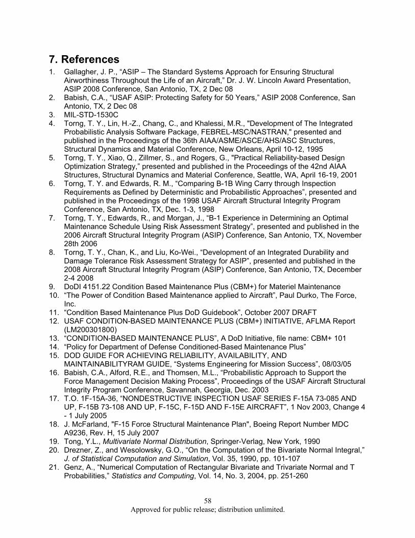
58 Approved for public release; distribution unlimited.
7. References 1. Gallagher, J. P., “ASIP – The Standard Systems Approach for Ensuring Structural
Airworthiness Throughout the Life of an Aircraft,” Dr. J. W. Lincoln Award Presentation, ASIP 2008 Conference, San Antonio, TX, 2 Dec 08
2. Babish, C.A., “USAF ASIP: Protecting Safety for 50 Years,” ASIP 2008 Conference, San Antonio, TX, 2 Dec 08
3. MIL-STD-1530C 4. Torng, T. Y., Lin, H.-Z., Chang, C., and Khalessi, M.R., "Development of The Integrated
Probabilistic Analysis Software Package, FEBREL-MSC/NASTRAN," presented and published in the Proceedings of the 36th AIAA/ASME/ASCE/AHS/ASC Structures, Structural Dynamics and Material Conference, New Orleans, April 10-12, 1995
5. Torng, T. Y., Xiao, Q., Zillmer, S., and Rogers, G., "Practical Reliability-based Design Optimization Strategy,” presented and published in the Proceedings of the 42nd AIAA Structures, Structural Dynamics and Material Conference, Seattle, WA, April 16-19, 2001
6. Torng, T. Y. and Edwards, R. M., “Comparing B-1B Wing Carry through Inspection Requirements as Defined by Deterministic and Probabilistic Approaches”, presented and published in the Proceedings of the 1998 USAF Aircraft Structural Integrity Program Conference, San Antonio, TX, Dec. 1-3, 1998
7. Torng, T. Y., Edwards, R., and Morgan, J., “B-1 Experience in Determining an Optimal Maintenance Schedule Using Risk Assessment Strategy”, presented and published in the 2006 Aircraft Structural Integrity Program (ASIP) Conference, San Antonio, TX, November 28th 2006
8. Torng, T. Y., Chan, K., and Liu, Ko-Wei., “Development of an Integrated Durability and Damage Tolerance Risk Assessment Strategy for ASIP”, presented and published in the 2008 Aircraft Structural Integrity Program (ASIP) Conference, San Antonio, TX, December 2-4 2008
9. DoDI 4151.22 Condition Based Maintenance Plus (CBM+) for Materiel Maintenance 10. “The Power of Condition Based Maintenance applied to Aircraft”, Paul Durko, The Force,
Inc. 11. “Condition Based Maintenance Plus DoD Guidebook”, October 2007 DRAFT 12. USAF CONDITION-BASED MAINTENANCE PLUS (CBM+) INITIATIVE, AFLMA Report
(LM200301800) 13. “CONDITION-BASED MAINTENANCE PLUS”, A DoD Initiative, file name: CBM+ 101 14. “Policy for Department of Defense Conditioned-Based Maintenance Plus” 15. DOD GUIDE FOR ACHIEVING RELIABILITY, AVAILABILITY, AND
MAINTAINABILITYRAM GUIDE, “Systems Engineering for Mission Success”, 08/03/05 16. Babish, C.A., Alford, R.E., and Thomsen, M.L., “Probabilistic Approach to Support the
Force Management Decision Making Process”, Proceedings of the USAF Aircraft Structural Integrity Program Conference, Savannah, Georgia, Dec. 2003
17. T.O. 1F-15A-36, “NONDESTRUCTIVE INSPECTION USAF SERIES F-15A 73-085 AND UP, F-15B 73-108 AND UP, F-15C, F-15D AND F-15E AIRCRAFT”, 1 Nov 2003, Change 4 - 1 July 2005
18. J. McFarland, "F-15 Force Structural Maintenance Plan", Boeing Report Number MDC A9236, Rev. H, 15 July 2007
19. Tong, Y.L., Multivariate Normal Distribution, Springer-Verlag, New York, 1990 20. Drezner, Z., and Wesolowsky, G.O., “On the Computation of the Bivariate Normal Integral,”
J. of Statistical Computation and Simulation, Vol. 35, 1990, pp. 101-107 21. Genz, A., “Numerical Computation of Rectangular Bivariate and Trivariate Normal and T
Probabilities,” Statistics and Computing, Vol. 14, No. 3, 2004, pp. 251-260

59 Approved for public release; distribution unlimited.
22. Domyancic, L.C., and Millwater, H.R., “Advances in Bounding Techniques for Aircraft Structures,” AIAA Journal, Vol. 50, No. 5, 2012, pp. 1307-1313
23. Vanderplaats, G.N., and Sugimoto, H., “A General-Purpose Optimization Program for Engineering Design,” Computers and Structures, Vol. 24, No. 1, 1986, pp. 13-21
24. Domyancic, L.C., Smith, L., and Millwater, H.R., “A Fast First-Order Method for Filtering Limit States,” 50th AIAA/ASME/ASCE/AHS/ASC Structures, Structural Dynamics, and Materials Conf., 2009
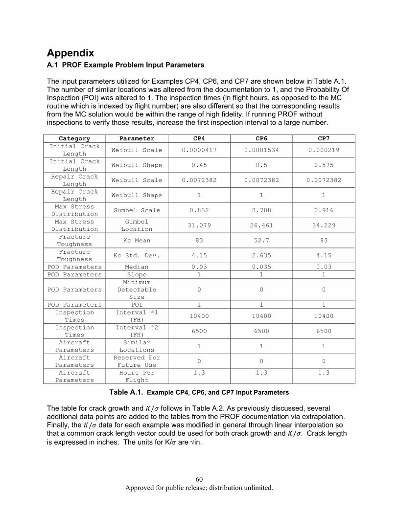
60 Approved for public release; distribution unlimited.
Appendix A.1 PROF Example Problem Input Parameters The input parameters utilized for Examples CP4, CP6, and CP7 are shown below in Table A.1. The number of similar locations was altered from the documentation to 1, and the Probability Of Inspection (POI) was altered to 1. The inspection times (in flight hours, as opposed to the MC routine which is indexed by flight number) are also different so that the corresponding results from the MC solution would be within the range of high fidelity. If running PROF without inspections to verify those results, increase the first inspection interval to a large number.
Category Parameter CP4 CP6 CP7 Initial Crack
Length Weibull Scale 0.0000417 0.0001534 0.000219
Initial Crack Length Weibull Shape 0.45 0.5 0.575
Repair Crack Length Weibull Scale 0.0072382 0.0072382 0.0072382
Repair Crack Length Weibull Shape 1 1 1
Max Stress Distribution Gumbel Scale 0.832 0.708 0.916
Max Stress Distribution
Gumbel Location 31.079 26.461 34.229
Fracture Toughness Kc Mean 83 52.7 83
Fracture Toughness Kc Std. Dev. 4.15 2.635 4.15
POD Parameters Median 0.03 0.035 0.03 POD Parameters Slope 1 1 1
POD Parameters Minimum
Detectable Size
0 0 0
POD Parameters POI 1 1 1 Inspection
Times Interval #1
(FH) 10400 10400 10400
Inspection Times
Interval #2 (FH) 6500 6500 6500
Aircraft Parameters
Similar Locations 1 1 1
Aircraft Parameters
Reserved For Future Use 0 0 0
Aircraft Parameters
Hours Per Flight
1.3
1.3
1.3
Table A.1. Example CP4, CP6, and CP7 Input Parameters
The table for crack growth and 𝐾/𝜎 follows in Table A.2. As previously discussed, several additional data points are added to the tables from the PROF documentation via extrapolation. Finally, the 𝐾/𝜎 data for each example was modified in general through linear interpolation so that a common crack length vector could be used for both crack growth and 𝐾/𝜎. Crack length is expressed in inches. The units for K/σ are √in.

61 Approved for public release; distribution unlimited.
CP4 CP6 CP7 FH Crack K/σ Crack K/σ Crack K/σ 0 1E-20 1E-20 1E-20 1E-20 1E-20 1E-20
500 0.0001 0.00638 0.0001 0.0050375 0.0001 0.00635 1000 0.0001636 0.01043768 0.00015 0.00755625 0.0001587 0.01007745 1500 0.0002093 0.01335334 0.0001838 0.009258925 0.0002 0.0127 2000 0.0002678 0.01708564 0.0002251 0.01133941 0.0002519 0.01599565 2500 0.0003425 0.0218515 0.0002757 0.01388839 0.0003174 0.0201549 3000 0.0004382 0.02795716 0.0003377 0.01701164 0.0003999 0.02539365 3500 0.0005605 0.0357599 0.0004137 0.02084014 0.0005038 0.0319913 4000 0.000717 0.0457446 0.0005067 0.02552501 0.0006347 0.04030345 4500 0.0009171 0.05851098 0.0006207 0.03126776 0.0007997 0.05078095 5000 0.001173 0.0748374 0.0007602 0.03829508 0.001007 0.0639445 5500 0.001501 0.0957638 0.0009312 0.0469092 0.001269 0.0805815 6000 0.00192 0.122496 0.001141 0.05747788 0.001599 0.1015365 6500 0.002456 0.1566928 0.001397 0.07037388 0.002015 0.1279525 7000 0.003141 0.2003958 0.001711 0.08619163 0.002538 0.161163 7500 0.004019 0.2564122 0.002096 0.105586 0.003198 0.203073 8000 0.00514 0.32166 0.002568 0.129363 0.004029 0.2558415 8500 0.006576 0.354992 0.003145 0.1584294 0.005075 0.31945 9000 0.008411 0.402631 0.003852 0.1940445 0.006394 0.351577 9500 0.01076 0.44864 0.004718 0.2376693 0.008056 0.38604 10000 0.01376 0.51282 0.005779 0.2911171 0.01015 0.44248125 10500 0.01761 0.57876 0.007079 0.3566046 0.01279 0.49495125 11000 0.02252 0.6541067 0.008671 0.417762 0.01611 0.55334025 11500 0.02881 0.7344 0.01062 0.46736 0.0203 0.6215325 12000 0.03686 0.7880667 0.01301 0.509185 0.02557 0.67681395 12500 0.04715 0.7961333 0.01594 0.56668 0.03221 0.72817435 13000 0.06031 0.80831 0.01952 0.63536 0.04059 0.79299365 13500 0.07715 0.8261773 0.02391 0.712425 0.05113 0.81335868 14000 0.09868 0.85235 0.02928 0.74128 0.06442 0.82712712 14500 0.1262 0.8879143 0.03587 0.76132 0.08116 0.848305655 15000 0.1615 0.9354722 0.04394 0.78333 0.1023 0.873075323 15500 0.2066 0.9944696 0.05382 0.8095371 0.1288 0.895685806 16000 0.2642 1.064338 0.06592 0.8423 0.1623 0.9361445 16500 0.338 1.248293 0.08074 0.8760889 0.2045 1.032826923 17000 0.4324 1.331211 0.0909 0.8970909 0.2576 1.115005 17500 0.5531 1.45627 0.1211 1.022631 0.3245 1.29965 18000 0.7075 1.64748 0.1484 1.041894 0.4089 1.455712364 18500 0.9051 1.89219 0.1818 1.066789 0.5151 1.664574773 19000 NA NA 0.2226 1.099343 0.640562043 1.920916538 19500 NA NA 0.2727 1.142988 0.795404296 2.237287414 20000 NA NA 0.334 1.202 0.9829513 2.620480043 20500 NA NA 0.4091 1.284922 NA NA 21000 NA NA 0.5011 1.419031 NA NA 21500 NA NA 0.6138 1.651258 NA NA 22000 NA NA 0.6657 1.770237 NA NA
Table A.2. Example CP4, CP6, and CP7 Crack Growth and K/σ Data

62 Approved for public release; distribution unlimited.
Acronyms, Symbols and Abbreviations
CBA Cost Benefit Analysis
CBM+SI Condition-Based Maintenance Plus Structural Integrity
CP Control Point
DC Durability Critical Aircraft part(s)
DIR Directly-Tracked aircraft part
DTA Damage Tolerance Analysis/Assessment
FSMP Force Structural Maintenance Plan
FST Full-Scale Test
FUA Financial Uncertainty Analysis
IATP Individual Aircraft Tracking Program
IFFC Inflight Failure Cost
IND Indirectly-Tracked Aircraft Part
IND(L) Indirectly-Tracked Aircraft Part linked to a directly-tracked part
INS In-Service
LCC Life Cycle Costs
LCRT Large Crack Replacement Time
MCRT Medium Crack Repair Time
MMH Maintenance Man Hours
MOQS Maintenance Operational Query System
NDE Non-Destructive Evaluation
NDI Non-Destructive Inspection
NMC Non-Mission Capable
%NMC % Fleet Non-Mission Capable
NPV NET-Present Value
PRC Part Replacement Cost
PROF Probability of Failure; Air Force code used to determine Risk of a part(s)
POD Probability of Detection
RBDMS Risk-Based Design & Maintenance System; Boeing code used to determine Risk of a part(s)
REMIS Air Force’s Reliability and Maintenance Information System

63 Approved for public release; distribution unlimited.
ROI Return on Investment
SCRT Small Crack Repair Time
SFPOF Single Point Probability of Failure
SHM Structural Health Monitoring
SME Subject Matter Expert
TPM Technical Performance Measurements
WUC Work Unit Code