Air Traffic Control Resource Management Strategies and the ...
246
Air Traffic Control Resource Management Strategies and the Small Aircraft Transportation System: A System Dynamics Perspective by James J. Galvin Jr. Dissertation submitted to the Faculty of the Virginia Polytechnic Institute and State University towards fulfillment of the requirements for the degree of Doctor of Philosophy in Industrial and Systems Engineering C. Patrick Koelling, Chair Kimberly P. Ellis Brian M. Kleiner Steven E. Markham Antonio A. Trani December 2, 2002 Blacksburg, Virginia Keywords: Air Traffic Control, Small Aircraft Transportation System, System Dynamics Copyright 2002, James J. Galvin Jr.
Transcript of Air Traffic Control Resource Management Strategies and the ...
Air Traffic Control Resource Management Strategies and the Small
Aircraft Transportation System: A System Dynamics Perspective
by
James J. Galvin Jr.
Dissertation submitted to the Faculty of the Virginia Polytechnic Institute and State University
towards fulfillment of the requirements for the degree of
Doctor of Philosophy in
Industrial and Systems Engineering
C. Patrick Koelling, Chair Kimberly P. Ellis Brian M. Kleiner
Steven E. Markham Antonio A. Trani
December 2, 2002
Blacksburg, Virginia
Keywords: Air Traffic Control, Small Aircraft Transportation System, System Dynamics
Copyright 2002, James J. Galvin Jr.
Air Traffic Control Resource Management Strategies and the Small
Aircraft Transportation System: A System Dynamics Perspective
James J. Galvin Jr.
(ABSTRACT)
The National Aeronautics and Space Administration (NASA) is leading a research effort
to develop a Small Aircraft Transportation System (SATS) that will expand air transportation
capabilities to hundreds of underutilized airports in the United States. Most of the research effort
addresses the technological development of the small aircraft as well as the systems to manage
airspace usage and surface activities at airports. The Federal Aviation Administration (FAA)
will also play a major role in the successful implementation of SATS, however, the
administration is reluctant to embrace the unproven concept.
The purpose of the research presented in this dissertation is to determine if the FAA can
pursue a resource management strategy that will support the current radar-based Air Traffic
Control (ATC) system as well as a Global Positioning Satellite (GPS)-based ATC system
required by the SATS. The research centered around the use of the System Dynamics modeling
methodology to determine the future behavior of the principle components of the ATC system
over time.
The research included a model of the ATC system consisting of people, facilities,
equipment, airports, aircraft, the FAA budget, and the Airport and Airways Trust Fund. The
model generated system performance behavior used to evaluate three scenarios. The first
scenario depicted the base case behavior of the system if the FAA continued its current resource
management practices. The second scenario depicted the behavior of the system if the FAA
emphasized development of GPS-based ATC systems. The third scenario depicted a combined
resource management strategy that supplemented radar systems with GPS systems.
The findings of the research were that the FAA must pursue a resource management
strategy that primarily funds a radar-based ATC system and directs lesser funding toward a GPS-
based supplemental ATC system. The most significant contribution of this research was the
insight and understanding gained of how several resource management strategies and the
presence of SATS aircraft may impact the future US Air Traffic Control system.

iii
Dedication
I dedicate this work to my wife and daughters, three special people who accompanied me
throughout the dissertation journey. Their love, support and understanding served as an endless
source of energy that inspired me to persevere.
Regina, Shelby and Olivia – you are a blessing. Thank you.

iv
Acknowledgements
Completing a Doctoral Dissertation is a group effort. As my academic advisor and
dissertation committee chairman, Pat Koelling was a prominent member of the wonderful group
of people who helped me to complete my dissertation. I thank Pat for his guidance, support and
enthusiasm. I also thank my committee members, Kimberly Ellis, Brian Kleiner, Steve
Markham, and Toni Trani for their advice and dedication of time and talent to this endeavor. I
also wish to thank Professors Harold Kurstedt and Eileen Van Aken for their tutelage and
friendship. I thank my fellow graduate students Rick Groesbeck, Tom McDonald, and Bret
Swan for their advice and support during my three years on campus. Finally, I thank and
acknowledge the Officers and Soldiers I serve with in the US Army who gave me the
opportunity to continue my education at this point in my military career.
Contents
Chapter 1: Introduction ..................................................................................... 1 1.1 Challenges for Air Traffic Control.................................................................................. 1 1.2 Research Purpose ............................................................................................................ 2 1.3 Research Objective.......................................................................................................... 3 1.4 Research Questions ......................................................................................................... 3 1.5 Hypothesized System Behavior Over Time .................................................................... 4 1.6 Research Contribution..................................................................................................... 5 1.7 Outline of Document....................................................................................................... 6
Chapter 2: Literature Review............................................................................ 7 2.1 The Vision of a Small Aircraft Transportation System................................................... 7 2.2 The FAA Goal of Free Flight........................................................................................ 10 2.3 A Brief History of Air Traffic Control.......................................................................... 14 2.4 Anticipated Air Traffic Control Requirements and Initiatives...................................... 16 2.5 Air Traffic Controller Functions and Tools .................................................................. 18
2.5.1 Preflight................................................................................................................. 19 2.5.2 Takeoff .................................................................................................................. 19 2.5.3 Departure............................................................................................................... 19 2.5.4 Enroute .................................................................................................................. 20 2.5.5 Approach ............................................................................................................... 20 2.5.6 Landing.................................................................................................................. 20
2.6 SATS Modeling at Virginia Tech ................................................................................. 21 2.7 The FAA Strategic Decision Support System Model ................................................... 22 2.8 European Shortages of Air Traffic Controllers ............................................................. 23 2.9 Preview: A System Dynamics Approach to Air Traffic Control Manpower and Infrastructure Modeling............................................................................................................. 24 2.10 Systems Thinking and the Systems Approach .............................................................. 26 2.11 System Dynamics.......................................................................................................... 29 2.12 System Dynamics Terminology and Tools ................................................................... 31
2.12.1 Fundamental Concepts of System Dynamics........................................................ 31 2.12.2 System Dynamics Modeling Tools ....................................................................... 35
2.13 Why Use System Dynamics.......................................................................................... 37 2.14 The System Dynamics Modeling Process..................................................................... 39
2.14.1 Ford’s Eight-step System Dynamics Modeling Process ....................................... 40 2.14.2 Sterman’s Five-step System Dynamics Modeling Process ................................... 44
2.15 Model Validity .............................................................................................................. 46 2.15.1 Maani and Cavana’s Policy, Strategy, and Scenario Approach............................ 51
2.16 System Archetypes........................................................................................................ 56 2.16.1 The Limits to Growth Archetype .......................................................................... 57 2.16.2 The Tragedy of the Commons Archetype ............................................................. 58 2.16.3 The Success to the Successful Archetype ............................................................. 60
2.17 System Dynamics Software .......................................................................................... 61 2.18 Summary ....................................................................................................................... 63

vi
Chapter 3: Research Design ............................................................................ 65 3.1 Research Design Overview ........................................................................................... 65 3.2 The System Dynamics Modeling Process..................................................................... 66
3.2.1 Step 1: Problem Definition.................................................................................... 66 3.2.2 Step 2: System Description ................................................................................... 67 3.2.3 Step 3: Build a Simulation Model ......................................................................... 68 3.2.4 Step 4: Validate the Model.................................................................................... 69
3.3 Computer Simulation Experimentation......................................................................... 71 3.3.1 Step 5: Establish a Base Case................................................................................ 71 3.3.2 Step 6: Conduct Policy Experiments..................................................................... 72 3.3.3 Step 7: Conduct Strategy Experiments.................................................................. 72 3.3.4 Step 8: Conduct Scenario Analysis ....................................................................... 72 3.3.5 Additional Considerations for Policy, Strategy, and Scenario Alternatives ......... 73 3.3.6 Step 9: Implement New Policies and Structure..................................................... 73
3.4 Treatment of the Data.................................................................................................... 73 3.4.1 Data Requirements ................................................................................................ 74 3.4.2 Data Management ................................................................................................. 75 3.4.3 Data Analysis ........................................................................................................ 75
3.5 Expected Results ........................................................................................................... 75
Chapter 4: The ATC Resource Management Model .................................... 77 4.1 System Dynamics Model Development Process........................................................... 77 4.2 Levels of analysis .......................................................................................................... 77
4.2.1 The Level of Theory.............................................................................................. 79 4.2.2 Entities and Variables............................................................................................ 79
4.3 Model Overview............................................................................................................ 80 4.3.1 Model Conceptualization ...................................................................................... 82 4.3.2 Delays and Feedback loops ................................................................................... 83 4.3.3 Modeling Assumptions ......................................................................................... 84 4.3.4 Modeling Objectives ............................................................................................. 85
4.4 Modeling ATC Resource Management Strategies........................................................ 85 4.4.1 Strategy 1: Maintain the Radar-based System ...................................................... 85 4.4.2 Strategy 2: Reduce the Radar-based System......................................................... 86 4.4.3 Strategy 3: Supplement the Radar-based System.................................................. 86 4.4.4 ATC Resource Management Policies ................................................................... 86 4.4.5 Exogenous Input into the System and the Model.................................................. 87
4.5 Model subsystems ......................................................................................................... 88 4.6 The People Subsystem .................................................................................................. 88
4.6.1 FAA Employee Job Descriptions.......................................................................... 90 4.6.2 Modeling the People Subsystem ........................................................................... 91 4.6.3 People Subsystem Stock & Flow Diagrams.......................................................... 94
4.7 The FAA Budget Subsystem......................................................................................... 95 4.7.1 Expenditures: The FAA Budget............................................................................ 96 4.7.2 Improving Airports: The Grants-in-Aid Account ................................................. 97 4.7.3 Supporting People: The Operations Account........................................................ 99 4.7.4 Providing Infrastructure: The Facilities and Equipment Account ...................... 104 4.7.5 ATC Revenue: The Airport and Airway Trust Fund .......................................... 108

vii
4.7.6 Budget Subsystem Stock & Flow Diagram......................................................... 111 4.8 The Facilities and Equipment Subsystem ................................................................... 111
4.8.1 Centers, Approach Controls, and Flight Service Stations................................... 112 4.8.2 Control Towers.................................................................................................... 113 4.8.3 Control Towers Stock and Flow diagrams.......................................................... 121
4.9 The Equipment Subsystem.......................................................................................... 122 4.9.1 ATC Radar Equipment........................................................................................ 122 4.9.2 ATC GPS Equipment .......................................................................................... 125
4.10 The Airports Subsystem.............................................................................................. 125 4.11 The Aircraft Subsystem............................................................................................... 127 4.12 Summary ..................................................................................................................... 131
Chapter 5: Model Verification and Validation............................................ 132 5.1 Verification.................................................................................................................. 132
5.1.1 Use Vensim Verification Tools........................................................................... 132 5.1.2 Run the model on a second computer ................................................................. 133 5.1.3 Trace numerical values through the system ........................................................ 133
5.2 Validation .................................................................................................................... 135 5.2.1 Model simplicity ................................................................................................. 135 5.2.2 Adherence to Physical Laws ............................................................................... 139 5.2.3 Adherence to Decision-making procedures ........................................................ 139 5.2.4 Absence of “fudge factors” ................................................................................. 139 5.2.5 Model Parameter Checks .................................................................................... 140 5.2.6 Face Validity ....................................................................................................... 146 5.2.7 Extreme Values Testing ...................................................................................... 146 5.2.8 Time Step Testing ............................................................................................... 147 5.2.9 Behavior Reproduction Testing .......................................................................... 149 5.2.10 Behavior Anomaly Testing ................................................................................. 153 5.2.11 Sensitivity Analysis............................................................................................. 154
5.3 Summary ..................................................................................................................... 159
Chapter 6: Simulation, Analysis, and Results.............................................. 160 6.1 Three ATC Scenarios .................................................................................................. 161
6.1.1 Scenario 1: Maintain the Radar-Based System................................................... 161 6.1.2 Scenario 2: Maximize funding for the GPS-Based System ................................ 162 6.1.3 Scenario 3: Supplement the Radar-Based System .............................................. 163
6.2 Scenario 1: Simulation and Analysis of the Radar-based System .............................. 164 6.2.1 Simulation of the Radar-based System ............................................................... 164 6.2.2 Analysis of Scenario 1......................................................................................... 175
6.3 Scenario 2: Simulation and Analysis of the GPS-based System................................. 178 6.3.1 Simulation of the GPS-based System.................................................................. 178 6.3.2 Analysis of Scenario 2......................................................................................... 190
6.4 Scenario 3: Simulation and Analysis of the radar-based system supplemented by GPS 192
6.4.1 Simulation of the radar-based system supplemented by GPS............................. 192 6.4.2 Analysis of Scenario 3......................................................................................... 203
6.5 Summary of Simulation, Analysis, and Results.......................................................... 206

viii
6.5.1 Research Question 1: Future levels of support for SATS under radar-based ATC 206 6.5.2 Research Question 2: Future levels of support for SATS under an aggressive transition to GPS-based ATC.............................................................................................. 206 6.5.3 Research Question 3: Future levels of support for SATS under a radar-based ATC system supplemented by GPS ............................................................................................. 207
Chapter 7: Conclusion.................................................................................... 209 7.1 Major Findings ............................................................................................................ 209 7.2 Research Questions ..................................................................................................... 210 7.3 Future FAA Resource Management Strategies........................................................... 210 7.4 Future Considerations for SATS Proponents .............................................................. 212 7.5 Future Research........................................................................................................... 213 7.6 Summary ..................................................................................................................... 213
References ............................................................................................................ 214
Appendix 1: Glossary.......................................................................................... 219
Appendix 2: Control Tower Rankings .............................................................. 220
ix
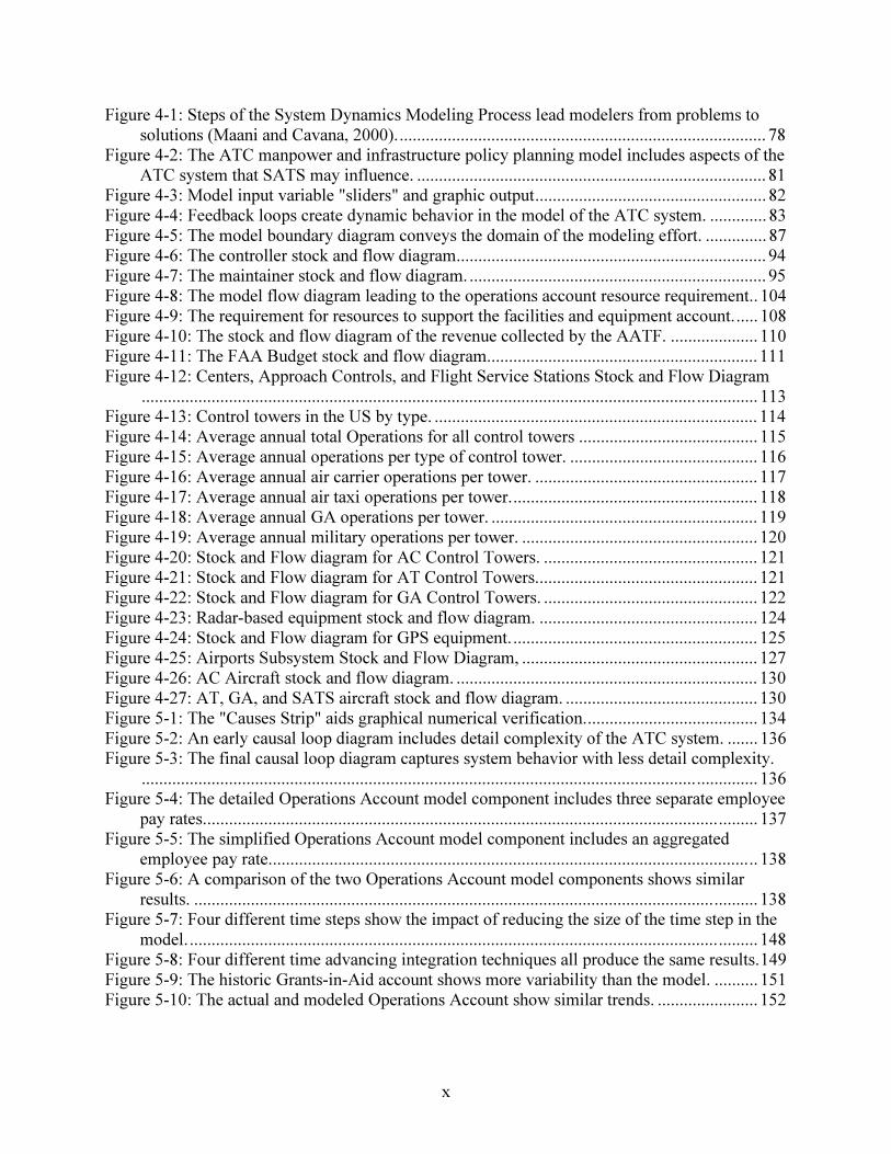
List of Figures Figure 1-1: Alternative policies implemented by resource managers will influence the number of
SATS aircraft the ATC system will support. .......................................................................... 4 Figure 2-1. Approximately 5,400 public use airports can support SATS precision landings
(Adapted from Holmes, 2000a)............................................................................................... 8 Figure 2-2. A constraint to the current airspace system is that there are approximately 700
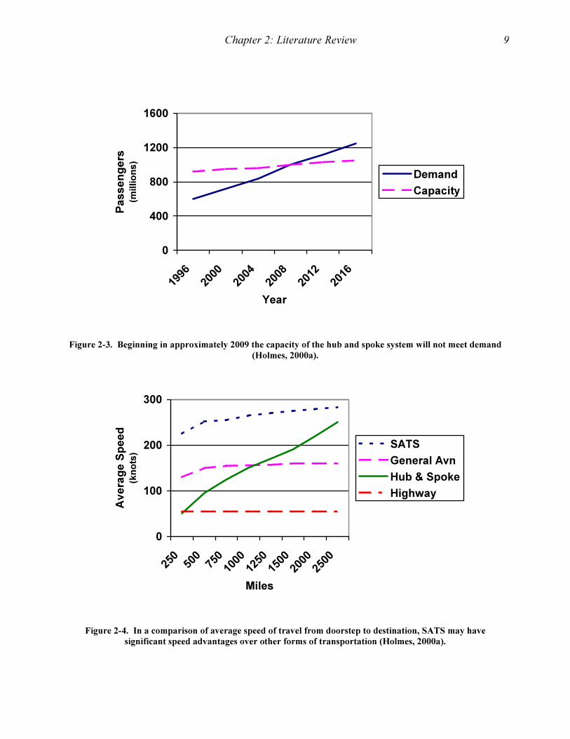
airports suitable for precision instrument landings (Adapted from Holmes, 2000a). ............. 8 Figure 2-3. Beginning in approximately 2009 the capacity of the hub and spoke system will not
meet demand (Holmes, 2000a)................................................................................................ 9 Figure 2-4. In a comparison of average speed of travel from doorstep to destination, SATS may
have significant speed advantages over other forms of transportation (Holmes, 2000a). ...... 9 Figure 2-5. In the current air traffic control system voice commands and transmissions from
ground-based navigation aids provide the primary means of navigation and conflict avoidance in predefined air corridors.................................................................................... 12
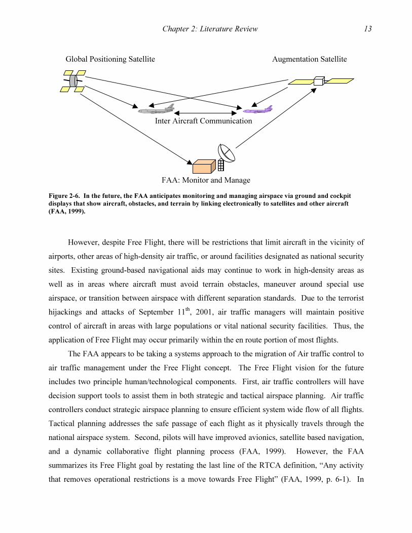
Figure 2-6. In the future, the FAA anticipates monitoring and managing airspace via ground and cockpit displays that show aircraft, obstacles, and terrain by linking electronically to satellites and other aircraft (FAA, 1999)............................................................................... 13
Figure 2-7. A simple model of the flow of air traffic controllers................................................. 25 Figure 2-8. An expanded depiction of Figure 2-7 where the controller stock consists of tower,
TRACON, and center controllers and administrators. .......................................................... 26 Figure 2-9. Four views of equilibrium (Ford, 1999). ................................................................... 38 Figure 2-10. Forrester’s 6-step model of the System Dynamics process shows the role of
feedback and indicates the need for frequent iteration of the process (Forrester, 1994). ..... 40 Figure 2-11. Of the three sources of data for the System Dynamics process, the greatest source
of the most useful information comes from the mental database (Forrester, 1991).............. 42 Figure 2-12. The limits to growth archetype consist of growth through the reinforcing loop on
the left counteracted by the balancing loop on the right, which has a vertical mark indicating a delay. .................................................................................................................................. 57
Figure 2-13. The typical pattern of behavior caused by the limits to growth system archetype includes a period of favorable behavior followed by a plateau or deterioration................... 58
Figure 2-14. The tragedy of the commons archetype consists of growing individual airlines, depicted in the upper and lower reinforcing loops, constrained by the common resource of airspace available in the national system. ............................................................................. 59
Figure 2-15. The typical pattern of behavior caused by the tragedy of the commons system archetype includes a period of favorable behavior followed by a decline as more individual airlines compete for the same limited resource. .................................................................... 59
Figure 2-16. Since the airlines initially dominate, as depicted in the upper reinforcing loop, they continue to grow while the competing SATS declines. ........................................................ 60
Figure 2-17. The typical pattern of behavior caused by the success to the successful system archetype involves a divergence of performance as the airlines’ initial dominance feeds growth.................................................................................................................................... 61
Figure 3-1. The research design is a plan to develop the model, test the model, use the model for policy and strategy experimentation, and conduct scenario analysis.................................... 65
x
Figure 4-1: Steps of the System Dynamics Modeling Process lead modelers from problems to solutions (Maani and Cavana, 2000)..................................................................................... 78
Figure 4-2: The ATC manpower and infrastructure policy planning model includes aspects of the ATC system that SATS may influence. ................................................................................ 81
Figure 4-3: Model input variable "sliders" and graphic output..................................................... 82 Figure 4-4: Feedback loops create dynamic behavior in the model of the ATC system. ............. 83 Figure 4-5: The model boundary diagram conveys the domain of the modeling effort. .............. 87 Figure 4-6: The controller stock and flow diagram....................................................................... 94 Figure 4-7: The maintainer stock and flow diagram. .................................................................... 95 Figure 4-8: The model flow diagram leading to the operations account resource requirement.. 104 Figure 4-9: The requirement for resources to support the facilities and equipment account...... 108 Figure 4-10: The stock and flow diagram of the revenue collected by the AATF. .................... 110 Figure 4-11: The FAA Budget stock and flow diagram.............................................................. 111 Figure 4-12: Centers, Approach Controls, and Flight Service Stations Stock and Flow Diagram
............................................................................................................................................. 113 Figure 4-13: Control towers in the US by type. .......................................................................... 114 Figure 4-14: Average annual total Operations for all control towers ......................................... 115 Figure 4-15: Average annual operations per type of control tower. ........................................... 116 Figure 4-16: Average annual air carrier operations per tower. ................................................... 117 Figure 4-17: Average annual air taxi operations per tower......................................................... 118 Figure 4-18: Average annual GA operations per tower. ............................................................. 119 Figure 4-19: Average annual military operations per tower. ...................................................... 120 Figure 4-20: Stock and Flow diagram for AC Control Towers. ................................................. 121 Figure 4-21: Stock and Flow diagram for AT Control Towers................................................... 121 Figure 4-22: Stock and Flow diagram for GA Control Towers. ................................................. 122 Figure 4-23: Radar-based equipment stock and flow diagram. .................................................. 124 Figure 4-24: Stock and Flow diagram for GPS equipment......................................................... 125 Figure 4-25: Airports Subsystem Stock and Flow Diagram, ...................................................... 127 Figure 4-26: AC Aircraft stock and flow diagram. ..................................................................... 130 Figure 4-27: AT, GA, and SATS aircraft stock and flow diagram. ............................................ 130 Figure 5-1: The "Causes Strip" aids graphical numerical verification........................................ 134 Figure 5-2: An early causal loop diagram includes detail complexity of the ATC system. ....... 136 Figure 5-3: The final causal loop diagram captures system behavior with less detail complexity.
............................................................................................................................................. 136 Figure 5-4: The detailed Operations Account model component includes three separate employee
pay rates............................................................................................................................... 137 Figure 5-5: The simplified Operations Account model component includes an aggregated
employee pay rate................................................................................................................ 138 Figure 5-6: A comparison of the two Operations Account model components shows similar
results. ................................................................................................................................. 138 Figure 5-7: Four different time steps show the impact of reducing the size of the time step in the
model................................................................................................................................... 148 Figure 5-8: Four different time advancing integration techniques all produce the same results.149 Figure 5-9: The historic Grants-in-Aid account shows more variability than the model. .......... 151 Figure 5-10: The actual and modeled Operations Account show similar trends. ....................... 152

xi
Figure 5-11: The historic Facilities and Equipment Account shows more variability than the model................................................................................................................................... 152
Figure 5-12: The actual and modeled FAA Budgets show the same trends. .............................. 153 Figure 5-13: The base year tax revenue per AC aircraft significantly influences the AATF. .... 157 Figure 5-14: The AATF is very sensitive to the salary of FAA employees. .............................. 157 Figure 5-15: The AATF is moderately sensitive to the number of maintainers in the ATC system.
............................................................................................................................................. 158 Figure 5-16: The AATF is barely sensitive to changes in the interest rate gained on uncommitted
revenue. ............................................................................................................................... 158 Figure 5-17: The base year tax revenue per AT, GA, and SATS aircraft has little influence on the
AATF. ................................................................................................................................. 159 Figure 6-1: The first scenario maintains the resource management practices of the current ATC
system.................................................................................................................................. 162 Figure 6-2: The resource management strategy for the second scenario attempts to rapidly
transition to GPS-based ATC.............................................................................................. 163 Figure 6-3: The third scenario attempts to strike a balance between growth of GPS-based ATC
and contiuity of the radar-based system.............................................................................. 163 Figure 6-4: Revenue generated by the Airport & Airways Trust Fund shows a general growth
trend..................................................................................................................................... 165 Figure 6-5: Future FAA budgets will continue to grow.............................................................. 166 Figure 6-6: Congress supplements the FAA budget when there are AATF shortfalls. .............. 166 Figure 6-7: Retirements cause an initial decline in the controller population. ........................... 167 Figure 6-8: The maintainer-training program eventually compensates for retirements.............. 168 Figure 6-9: Flight Service Stations continue a steady climb in number. .................................... 168 Figure 6-10: There are few locations to create more control towers for airliners....................... 169 Figure 6-11: Radar-based ATC will require more control towers at Air Taxi airports. ............. 169 Figure 6-12: General Aviation control towers will continue to grow in numbers. ..................... 170 Figure 6-13: The pool of radar-based equipment remains constant in the first scenario. ........... 170 Figure 6-14: The GPS-based equipment decommission rate eventually overtakes the installation
rate. ...................................................................................................................................... 171 Figure 6-15: Inherent constraints in the ATC system restrict the growth in the number of AC
aircraft. ................................................................................................................................ 172 Figure 6-16: The population of AT aircraft growth significantly in the first scenario. .............. 172 Figure 6-17: The number of GA aircraft grows continuously in a radar-based ATC system..... 173 Figure 6-18: The lack of GPS support precludes the growth of the SATS program. ................. 173 Figure 6-19: Non-SATS airports decline at a rate of approximately two per month.................. 174 Figure 6-20: A modest growth rate creates a handful of SATS airports in the first scenario. .... 174 Figure 6-21: The Control Tower growth rate declines from that of the 1990s. .......................... 176 Figure 6-22: The decline in public use airports attributed to the growth in the aircraft/airports
ratio...................................................................................................................................... 176 Figure 6-23: The GPS-based approach in the second scenario generated less for the AATF
downstream. ........................................................................................................................ 180 Figure 6-24: The Future FAA budgets of the first and second scenario are very similar. .......... 180 Figure 6-25: The additional funding required by the second scenario may jeopardize its
implementation.................................................................................................................... 181

xii
Figure 6-26: The GPS-based approach to ATC requires controllers to enable the Hub and Spoke system.................................................................................................................................. 182
Figure 6-27: The reduction in radar-based equipment reduces the need for maintainers after 2012..................................................................................................................................... 183
Figure 6-28: Flight Service Stations continue to serve a larger audience due to the expansion of SATS. .................................................................................................................................. 183
Figure 6-29: The change in resource management causes a reduction in the population of AC towers. ................................................................................................................................. 184
Figure 6-30: An emphasis on GPS-based ATC will reduce the requirement for control towers at AT airports. ......................................................................................................................... 184
Figure 6-31: General Aviation control towers decline under the second scenario. .................... 185 Figure 6-32: The change in resource management causes a decline in the pool of radar-based
equipment. ........................................................................................................................... 185 Figure 6-33: The GPS-based equipment pool expands under the second scenario. ................... 186 Figure 6-34: Feedback from the GPS-based system further restrains the growth in the number of
AC aircraft........................................................................................................................... 187 Figure 6-35: The population of AT aircraft growth declines with the onset of SATS. .............. 187 Figure 6-36: The system converts many GA aircraft into SATS aircraft. .................................. 188 Figure 6-37: The growth of SATS airports enables the entire SATS program........................... 188 Figure 6-38: Non-SATS airports decline at a rate of approximately two per month.................. 189 Figure 6-39: The growth of SATS airports enables the entire SATS program........................... 189 Figure 6-40: The conversion of non-SATS airports into SATS airports begins in approximately
2012..................................................................................................................................... 191 Figure 6-41: Many AT and some GA aircraft convert into SATS aircraft. ................................ 191 Figure 6-42: The third scenario aligns closely with the first....................................................... 194 Figure 6-43: The Future FAA budgets of the first and third scenario are almost identical. ....... 194 Figure 6-44: The minimal additional funding required by the third scenario makes it feasible. 195 Figure 6-45: Each scenario requires controllers to support the Hub and Spoke system ATC
facilities. .............................................................................................................................. 196 Figure 6-46: The first and third scenarios require the same number of maintainers. ................. 196 Figure 6-47: There is a slight growth in the number of Flight Service Stations in the third
scenario................................................................................................................................ 197 Figure 6-48: The third scenario causes a slight reduction in the population of AC towers. ....... 197 Figure 6-49: The third scenario causes a slight reduction in the population of AT towers. ....... 198 Figure 6-50: General Aviation control towers decline slightly under the third scenario. ........... 198 Figure 6-51: The population of radar-based equipment remains high throughout the third
scenario................................................................................................................................ 199 Figure 6-52: The GPS-based equipment population provides minimal support for SATS. ....... 199 Figure 6-53: The third scenario maintains a steady population of AC aircraft........................... 200 Figure 6-54: The population of AT aircraft declines slightly with the onset of SATS after 2020 in
the third scenario. ................................................................................................................ 201 Figure 6-55: Only a small number of GA aircraft convert into SATS aircraft after 2024 in the
third scenario. ...................................................................................................................... 201 Figure 6-56: The third scenario delays the growth of SATS airports until five years after the
second scenario. .................................................................................................................. 202

xiii
Figure 6-57: The third scenario invokes a slightly accelerated decline of non-SATS airports after 2018..................................................................................................................................... 202
Figure 6-58: The third scenario shifts the growth of SATS airports five years later than the second scenario. .................................................................................................................. 203
Figure 6-59: The ratio of non-SATS aircraft to airports exceeds historical ranges after 2015... 205 Figure 6-60: The ratio of SATS aircraft to airports remains low beyond 2020. ......................... 205 Figure 7-1: The radar-based constraints limit AC revenue, GPS infrastructure, and ultimately,
SATS. .................................................................................................................................. 212
xiv
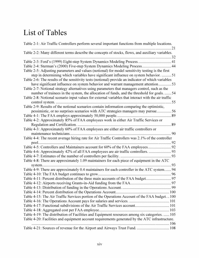
List of Tables
Table 2-1: Air Traffic Controllers perform several important functions from multiple locations.
............................................................................................................................................... 21 Table 2-2: Many different terms describe the concepts of stocks, flows, and auxiliary variables.
............................................................................................................................................... 32 Table 2-3: Ford’s (1999) Eight-step System Dynamics Modeling Process. ................................. 41 Table 2-4: Sterman’s (2000) Five-step System Dynamics Modeling Process.............................. 44 Table 2-5: Adjusting parameters and values (notional) for model sensitivity testing is the first
step in determining which variables have significant influence on system behavior. .......... 51 Table 2-6: The results of the sensitivity tests (notional) provide an indicator of which variables
have significant influence on system behavior and warrant management attention ............. 53 Table 2-7: Notional strategy alternatives using parameters that managers control, such as the
number of trainees in the system, the allocation of funds, and the threshold for goals. ....... 54 Table 2-8: Notional scenario input values for external variables that interact with the air traffic
control system. ...................................................................................................................... 55 Table 2-9: Results of the notional scenarios contain information comparing the optimistic,
pessimistic, or no surprises scenarios with ATC strategies managers may pursue............... 56 Table 4-1: The FAA employs approximately 50,000 people........................................................ 89 Table 4-2: Approximately 85% of FAA employees work in either Air Traffic Services or
Regulation and Certification. ................................................................................................ 89 Table 4-3: Approximately 60% of FAA employees are either air traffic controllers or
maintenance technicians........................................................................................................ 90 Table 4-4: The recent average hiring rate for Air Traffic Controllers was 2.1% of the controller
pool........................................................................................................................................ 92 Table 4-5: Controllers and Maintainers account for 60% of the FAA employees........................ 92 Table 4-6: Approximately 42% of all FAA employees are air traffic controllers. ....................... 93 Table 4-7: Estimates of the number of controllers per facility. .................................................... 93 Table 4-8: There are approximately 1.09 maintainers for each piece of equipment in the ATC
system.................................................................................................................................... 93 Table 4-9: There are approximately 0.4 maintainers for each controller in the ATC system....... 94 Table 4-10: The FAA budget continues to grow........................................................................... 96 Table 4-11: Percent distribution of the three main accounts of the FAA budget.......................... 97 Table 4-12: Airports receiving Grants-in-Aid funding from the FAA.......................................... 97 Table 4-13: Distribution of funding in the Operations Account. .................................................. 99 Table 4-14: Percent distribution of the Operations Account....................................................... 100 Table 4-15: The Air Traffic Services portion of the Operations Account of the FAA budget. .. 100 Table 4-16: The Operations Account pays for salaries and services. ......................................... 101 Table 4-17: Functional subdivisions of the Air Traffic Services account................................... 101 Table 4-18: Aggregated cost per FAA employee........................................................................ 103 Table 4-19: The distribution of Facilities and Equipment resources among six categories. ...... 105 Table 4-20: Facilities and equipment account requirements generated by the ATC infrastructure.
............................................................................................................................................. 106 Table 4-21: Sources of revenue for the Airport and Airways Trust Fund. ................................. 108
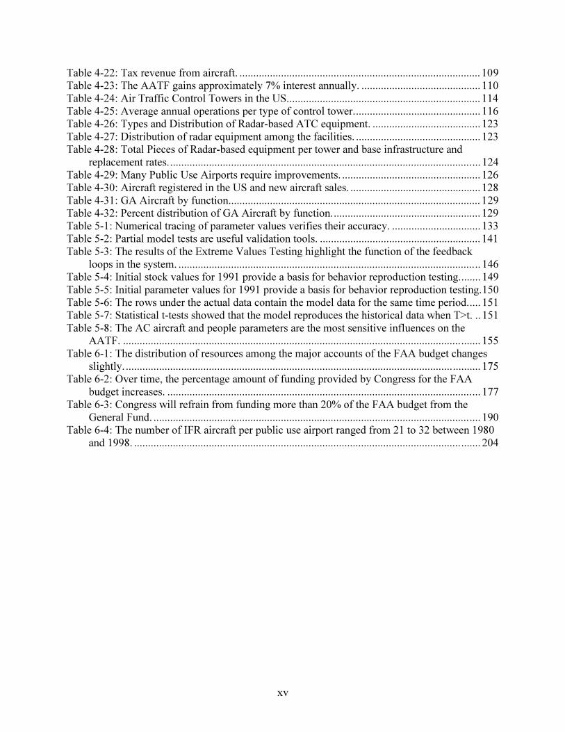
xv
Table 4-22: Tax revenue from aircraft. ....................................................................................... 109 Table 4-23: The AATF gains approximately 7% interest annually. ........................................... 110 Table 4-24: Air Traffic Control Towers in the US...................................................................... 114 Table 4-25: Average annual operations per type of control tower.............................................. 116 Table 4-26: Types and Distribution of Radar-based ATC equipment. ....................................... 123 Table 4-27: Distribution of radar equipment among the facilities. ............................................. 123 Table 4-28: Total Pieces of Radar-based equipment per tower and base infrastructure and
replacement rates................................................................................................................. 124 Table 4-29: Many Public Use Airports require improvements. .................................................. 126 Table 4-30: Aircraft registered in the US and new aircraft sales. ............................................... 128 Table 4-31: GA Aircraft by function........................................................................................... 129 Table 4-32: Percent distribution of GA Aircraft by function...................................................... 129 Table 5-1: Numerical tracing of parameter values verifies their accuracy. ................................ 133 Table 5-2: Partial model tests are useful validation tools. .......................................................... 141 Table 5-3: The results of the Extreme Values Testing highlight the function of the feedback
loops in the system. ............................................................................................................. 146 Table 5-4: Initial stock values for 1991 provide a basis for behavior reproduction testing........ 149 Table 5-5: Initial parameter values for 1991 provide a basis for behavior reproduction testing.150 Table 5-6: The rows under the actual data contain the model data for the same time period..... 151 Table 5-7: Statistical t-tests showed that the model reproduces the historical data when T>t. .. 151 Table 5-8: The AC aircraft and people parameters are the most sensitive influences on the
AATF. ................................................................................................................................. 155 Table 6-1: The distribution of resources among the major accounts of the FAA budget changes
slightly. ................................................................................................................................ 175 Table 6-2: Over time, the percentage amount of funding provided by Congress for the FAA
budget increases. ................................................................................................................. 177 Table 6-3: Congress will refrain from funding more than 20% of the FAA budget from the
General Fund. ...................................................................................................................... 190 Table 6-4: The number of IFR aircraft per public use airport ranged from 21 to 32 between 1980
and 1998. ............................................................................................................................. 204
1
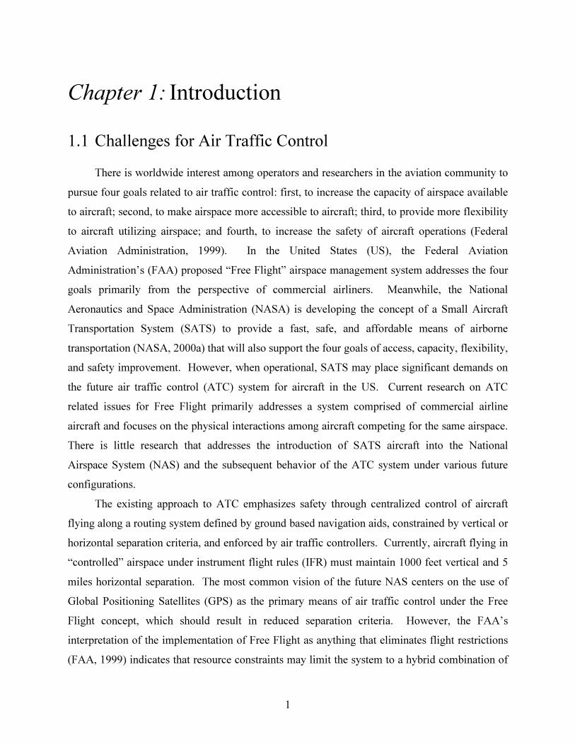
1.1 Challenges for Air Traffic Control
There is worldwide interest among operators and researchers in the aviation community to
pursue four goals related to air traffic control: first, to increase the capacity of airspace available
to aircraft; second, to make airspace more accessible to aircraft; third, to provide more flexibility
to aircraft utilizing airspace; and fourth, to increase the safety of aircraft operations (Federal
Aviation Administration, 1999). In the United States (US), the Federal Aviation
Administration’s (FAA) proposed “Free Flight” airspace management system addresses the four
goals primarily from the perspective of commercial airliners. Meanwhile, the National
Aeronautics and Space Administration (NASA) is developing the concept of a Small Aircraft
Transportation System (SATS) to provide a fast, safe, and affordable means of airborne
transportation (NASA, 2000a) that will also support the four goals of access, capacity, flexibility,
and safety improvement. However, when operational, SATS may place significant demands on
the future air traffic control (ATC) system for aircraft in the US. Current research on ATC
related issues for Free Flight primarily addresses a system comprised of commercial airline
aircraft and focuses on the physical interactions among aircraft competing for the same airspace.
There is little research that addresses the introduction of SATS aircraft into the National
Airspace System (NAS) and the subsequent behavior of the ATC system under various future
configurations.
The existing approach to ATC emphasizes safety through centralized control of aircraft
flying along a routing system defined by ground based navigation aids, constrained by vertical or
horizontal separation criteria, and enforced by air traffic controllers. Currently, aircraft flying in
“controlled” airspace under instrument flight rules (IFR) must maintain 1000 feet vertical and 5
miles horizontal separation. The most common vision of the future NAS centers on the use of
Global Positioning Satellites (GPS) as the primary means of air traffic control under the Free
Flight concept, which should result in reduced separation criteria. However, the FAA’s
interpretation of the implementation of Free Flight as anything that eliminates flight restrictions
(FAA, 1999) indicates that resource constraints may limit the system to a hybrid combination of
Chapter 1: Introduction

Chapter 1: Introduction 2
GPS and radar, as opposed to a complete transition to GPS. Thus, the implementation of some
level of GPS-based air traffic control systems combined with the need to maintain radar-based
ATC processes is likely to be a future challenge for air traffic controllers.
Besides the resource and implementation challenges of replacing radar with GPS, the
FAA may face the problem of integrating two complex systems – the ATC system and SATS.
One particular problem the administration must address is how the introduction of SATS aircraft
into the NAS will impact the FAA’s ability to conduct ATC under various combinations of GPS
and radar-based technology. Additionally, the introduction of SATS aircraft may adversely
influence the revenue collected to fund the ATC system through the Airport and Airways Trust
Fund (AATF). The development of SATS is currently in the concept development stage.
Research related to the integration of SATS and ATC at the macro system level is minimal.
Thus, there are opportunities to investigate potential scenarios to determine ATC system
behavior under various combinations of ATC and aircraft technologies.
1.2 Research Purpose
NASA is spending $69M on research to determine the feasibility of the SATS concept by
2005 (NASA, 2000). The Nimbus Corporation recently placed an order for 1,000 Eclipse 500
aircraft, which have operational characteristics similar to those of the SATS aircraft envisioned
by NASA (Eclipse Aviation, 2001). There is a great deal of industry and government
momentum to advance the use of small aircraft within the national transportation system.
However, there is limited research to determine how the introduction of SATS aircraft may
influence the FAA’s ATC system and how SATS may impact upon the flow of excise taxes
under future radar or GPS-based configurations. NASA proponents of SATS may argue that
SATS aircraft will be able to navigate entirely with their onboard systems and have little
influence on the ATC system. The SATS program objectives highlight capabilities such as self-
separation among aircraft through the use of advanced software and an airborne internet (NASA,
2000). However, it is highly likely that SATS aircraft will transit through airspace along with
less technologically capable aircraft, and, SATS aircraft will need to fly in airspace controlled by
human air traffic controllers.
Given the aforementioned developments and the fact that the FAA’s budget for 2001 was
approximately $12.5B (FAA, 2002a), of which more than $11B emanated from the AATF,
Chapter 1: Introduction 3
during the upcoming years government decision-makers will make important policy decisions
regarding the use of human and financial resources that will have long-term effects on the NAS.
The results of the research proposed in this document may offer new insights into the
development of policies related to the integration of SATS aircraft into the NAS by exposing the
feedback, causation, and implications of various ATC resource management policies.
It is infeasible to use real aircraft and an assortment of radar or GPS-based configurations
of an operating ATC system to conduct research on the macro-level behavior of the system over
time. Therefore, there is a need for an approach that uses a reasonable amount of resources, yet
remains a valid representation of the system under study. Computer simulation modeling of the
dynamic feedback within potential ATC system architectures offers an approach that meets these
criteria. In particular, the System Dynamics approach offers a combination of methodology and
tools to create and build a valid model of the principle components of an ATC system: people,
aircraft, facilities, equipment, airports, and their associated financial resources.
1.3 Research Objective
The objectives of the research outlined in this document are fourfold. The first goal of the
research is to determine how many SATS aircraft will be able to operate within the ATC system
under radar and GPS-based configurations. The second goal of the research is to gain
understanding of the dynamic behavior of the air traffic control system over time. The third goal
of the research is to contribute to a higher-level transportation system model of SATS being
developed at Virginia Tech. The fourth goal of the research is to contribute to the body of
knowledge used by FAA, NASA, and other SATS stakeholders and decision-makers.
The steps to achieve the objective are twofold: first, to create and validate a System
Dynamics computer simulation model of the ATC system; and second, to use the model to
evaluate three future scenarios under which SATS aircraft may operate within the NAS.
1.4 Research Questions
The following questions stem from the fundamental research question: what air traffic
control resource management strategy will support the future needs of the Small Aircraft
Transportation System and create adequate tax revenue to fund the Federal Aviation
Administration?
Chapter 1: Introduction 4
• Given the continuation of the current ground and radar-based ATC system, what level of
SATS flights will the system be able to support?
• Given a future transition period toward a GPS-based ATC system, what level of SATS
flights will the system be able to support?
• Given a future radar-based ATC system supplemented by a transition period to GPS,
what level of SATS flights will the system be able to support?
1.5 Hypothesized System Behavior Over Time
System Dynamics modeling will be useful to help interested parties understand the
behavior of the US ATC system as it evolves over time and attempts to accommodate SATS
aircraft. System Dynamics is an approach that addresses the relationships among the structure
and variables in a system. System Dynamics modeling is a process and a tool that shows how a
system continually adjusts itself over time to accommodate the policy alternatives decision-
makers may wish to implement. Researchers express System Dynamics “hypotheses” in terms
of “behavior over time” diagrams or “reference modes” to determine if a system may support
growth, decay, or some oscillating combination of the two (Ford, 1999; Sterman 2000). The
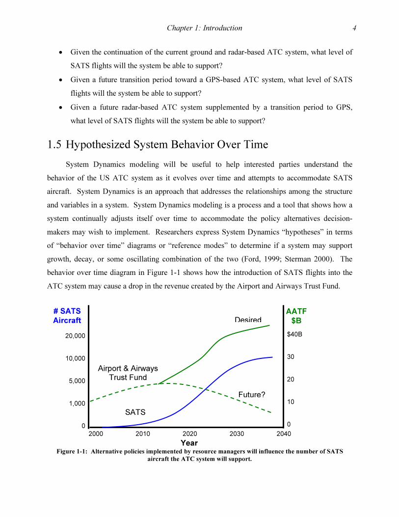
behavior over time diagram in Figure 1-1 shows how the introduction of SATS flights into the
ATC system may cause a drop in the revenue created by the Airport and Airways Trust Fund.
Figure 1-1: Alternative policies implemented by resource managers will influence the number of SATS
aircraft the ATC system will support.
$40B
30
20
10
0
Airport & Airways Trust Fund
SATS
Future?
# SATSAircraft
Year
2000 2010 2020 2030 2040
20,000
10,000
5,000
1,000
0
AATF $B Desired
Chapter 1: Introduction 5
Historically, the aviation industry in the US has shown continuous growth. The aircraft
inventory in the US grew from 76,549 in 1960 to 204,710 in 1998 (Bureau of Transportation
Statistics, 2002). Thus, the notional shape of the curve representing the number of SATS flights
over time in Figure 1-1 shows general patterns of growth. The challenge for ATC managers is to
support the growth of SATS flights, meet the demands of non-SATS aircraft, operate within the
resource constraints of the ATC system, and generate revenue for the AATF. The resource
constraints include the number of controllers, maintainers, facilities, airports, equipment, and
money available in the system. Resource managers of the ATC system should determine what
policies might cause the undesirable system behavior and what policies and strategies they may
use to create the desired system behavior. In this manner the System Dynamics approach serves
as a tool for learning and understanding the general behavior of systems (Ford, 1999).
1.6 Research Contribution
A rigorous investigation of the behavior of the ATC system under several radar and GPS-
based architectures will help to determine the potential level of participation of SATS aircraft in
the system. The research will address questions that remain unanswered in the academic
literature and are solely at the level of speculation and opinion within the practitioner literature.
The research may contribute to policy decision-making, further policy analysis, and continued
debate within the aviation community. The National Airspace System Architecture Version 4.0
(FAA, 1999) offers detailed plans for future air traffic control; however, it does not even address
the SATS. Meanwhile, the SATS Program Plan focuses on the vehicle technologies and does
not fully address the larger ATC infrastructure implications of SATS aircraft operating in the
NAS and potentially influencing the AATF. The research in this dissertation will serve as a
bridge between the FAA and NASA to show how the actions of the two administrations will
dynamically interact within the larger framework of the NAS. The results of the research may
provide findings that help the FAA to manage its resources to create the conditions that provide
an ATC system capable of meeting all of the demands of SATS and non-SATS aircraft.
The research expands the application of System Dynamics to government policy issues.
The System Dynamics approach is a valid methodology to offer insight into the potential impact
of SATS upon the ATC system. The approach will contribute to an ongoing System Dynamics
Chapter 1: Introduction 6
project at Virginia Tech. The application of the System Dynamics approach to issues important
to the aviation resource management community may encourage further use of System Dynamics
to address other pressing concerns in that community. The basic modeling approach will serve
as a framework to generalize the System Dynamics approach to further ATC studies and to the
widespread and diverse domain of government resource allocation problems in general.
1.7 Outline of Document
The remainder of the document consists of the following:
Chapter 2: The literature review includes the plans and objectives of NASA and the FAA,
a national-level overview of the current air traffic control system, a summary of related modeling
efforts, and a discussion of the System Dynamics modeling process: what it is, how to do it, how
to make it valid, how the approach is relevant for the research topic, and specific step-by-step
procedures to conduct the research.
Chapter 3: The research design stems from the System Dynamics model development and
refinement effort discussion presented in chapter 2. The nine-step methodology guides the
research effort through model development, validation, and application for policy analysis.
Chapter 4: The development of the model includes justification for all components of the
model, initial conditions, and the rational used to create various parameters used in model
equations.
Chapter 5: A variety of tests and procedures aid in verification and validation of the
model.
Chapter 6: The evaluation of the three basic scenarios provides results and information
useful to answer the research questions.
Chapter 7: The results and conclusions provide insight into the future of Air Traffic
Control and the Small Aircraft Transportation System as well as opportunities for further
research.
7
2.1 The Vision of a Small Aircraft Transportation System
In 2001 researchers at the National Aeronautics and Space Administration (NASA)
Langley Research Center began formal development of the concept of a Small Aircraft
Transportation System (SATS). They intend to demonstrate by 2005 whether or not the concept
works. They claim that, for distances of 800 miles or less, SATS will provide a faster, safer, and
more affordable means of airborne transportation than the current airline hub and spoke system.
They envision SATS aircraft operating out of the 5,400 public-use airports located throughout
the US as shown in Figure 2-1. The anticipated all-weather landing capabilities of SATS aircraft
represent a marked expansion in the accessibility of air travel throughout the US. Figure 2-2
depicts the approximately 700 airports with precision instrument landing systems that guide
aircraft to safe landings during periods of low ceilings or low visibility. Together the two figures
illustrate aspects of the vision statement articulated by the SATS program director, Dr. Bruce
Holmes, to guide researchers and developers associated with the SATS program: The small
aircraft transportation vision is a safe travel alternative freeing people and products from
transportation system delays, by creating access to more communities in less time (NASA,
2000a).
The SATS vision statement emphasizes safety, speed, and access. Clearly, Figure 2-1 and
Figure 2-2 demonstrate the potential increased geographic access SATS may provide.
Additionally, SATS may fill the gap projected in 2009 between the availability and demand for
hub and spoke flights indicated in Figure 2-3, thereby providing access simply by meeting
passenger demand. A NASA study of transportation system speed concluded that SATS has the
potential to greatly increase the average travel speed from doorstep to destination compared to
other forms of transportation (Holmes, 2000b). Figure 2-4 shows the results of the study and
indicates that SATS may provide far superior travel times. However, the safety of SATS
remains indeterminate until research shows the system’s feasibility as a safe form of air
transportation.
Chapter 2: Literature Review

Chapter 2: Literature Review 8
Figure 2-1. Approximately 5,400 public use airports can support SATS precision landings (Adapted from
Holmes, 2000a).
Figure 2-2. A constraint to the current airspace system is that there are approximately 700 airports suitable
for precision instrument landings (Adapted from Holmes, 2000a).
Chapter 2: Literature Review 9
0
400
800
1200
1600
1996
2000
2004
2008
2012
2016
Year
Passen
gers
(millions)
Demand
Capacity
Figure 2-3. Beginning in approximately 2009 the capacity of the hub and spoke system will not meet demand
(Holmes, 2000a).
0
100
200
300
250
500
750
1000
1250
1500
2000
2500
Miles
Avera
ge S
peed
(knots)
SATS
General Avn
Hub & Spoke
Highway
Figure 2-4. In a comparison of average speed of travel from doorstep to destination, SATS may have
significant speed advantages over other forms of transportation (Holmes, 2000a).
Chapter 2: Literature Review 10
The congressionally mandated research program for SATS includes four key operating
capabilities that NASA and the Federal Aviation Administration (FAA) must address. First, they
must demonstrate the feasibility of multiple aircraft operating in airspace around small airports
without control towers or radar surveillance. Second, they must demonstrate that aircraft can
conduct pinpoint landings in adverse weather without the use of ground based navigation aids.
Third, they must demonstrate that SATS aircraft can integrate with the en route airspace system
and with other aircraft. Fourth, they must demonstrate that single pilots of SATS aircraft can
function safely and competently in complex airspace (NASA, 2000b). However, due to
budgetary constraints, the NASA program managers have insufficient resources to fund research
for the third operating capability - integrating SATS into the en route airspace.
Despite the lack of funding for en route research, there remains a need to identify and
demonstrate the feasibility of ATC techniques using future technological capabilities available to
SATS aircraft and the managers of the NAS. Future technologies may allow a shift in control
from the centralized ATC system currently operated by the FAA to a decentralized system of
interacting aircraft conducting collaborative decision making to dynamically generate safe flight
paths (NASA, 2000a). Conceptually, SATS aircraft will communicate via an “airborne internet”
and will navigate using GPS to gain access to thousands of suburban, rural, and remote airfields.
The NASA proponents envision SATS aircraft using the airborne internet and GPS to operate
within the NAS under a concept called “Free Flight” (Federal Aviation Administration, 1999).
2.2 The FAA Goal of Free Flight
In the late 1990s the FAA, in concert with the aviation community, recognized four goals
related to airspace in order to increase the capacity, accessibility, and flexibility of airspace
available to aircraft while also contributing to the increased safety of aircraft operations (Federal
Aviation Administration, 1999). The proposed method of meeting the goals is through a concept
called “Free Flight.” The FAA accepts the definition of Free Flight advocated by the Radio
Technical Commission for Aeronautics (RTCA), a consortium of government and industry
organizations established in 1935 to build consensus among all members of the aviation
community regarding issues of mutual concern. The RTCA describes Free Flight as, “…a safe
and efficient operating capability under instrument flight rules in which the operators have the
freedom to select their path and speed in real time. Air traffic restrictions are imposed only to
Chapter 2: Literature Review 11
ensure separation, to preclude exceeding airport capability, to prevent unauthorized flight
through special use airspace, and to ensure safety of flight. Restrictions are limited in extent and
duration to correct the identified problem. Any activity which removes restrictions represents a
move toward Free Flight” (Federal Aviation Administration, 1999, p. 2-6). The Free Flight
description depicts the concept as an objective, not a specific system design. Additionally, the
description indicates that an incremental approach to Free Flight implementation is acceptable to
the aviation community. Among the reasons for adopting new approaches to air traffic
management, such as Free Flight, are to increase throughput at airports without building new
runways (Sastry, 1995) and to improve fuel consumption by making aircraft routing more
efficient (Chiang, 1997).
The FAA’s (1999) National Airspace Architecture Version 4.0 outlines the
administration’s approach to Free Flight. The FAA envisions a series of technological
innovations to incrementally modernize the ATC system. The FAA anticipates aircraft
navigation shifting from today’s ground and radar-based system of navigational aids, such as
radio beacons and transmitters, to satellite-based navigation and landing procedures. Aircraft
communications systems should transition from analogue to digital. Automated systems may
provide interactive flight planning to adjust flight routes prior to departure, they may monitor
and advise aircraft in flight, and they may create the conditions for a steady flow of air traffic
throughout the system. The FAA is devoting significant effort to transition to the systems it
envisions for the future. Currently, over 19,000 air traffic controllers use thousands of pieces of
equipment at hundreds of locations to manage the air traffic system. However, the infrastructure
is old, rapidly deteriorating, and in need of modernization (FAA, 1999, p. 2-3). Thus, the FAA’s
move to Free Flight involves a complex transition in personnel, technology, and procedures.
The changes associated with the use of airspace may entail a dramatic shift from a
philosophy of firm control to that of loose management. Figure 2-5 and Figure 2-6 graphically
show the physical and conceptual changes the FAA must undergo to transition from the current
radar-based system of air traffic control to the satellite-based Free Flight system of air traffic
management. Currently, aircraft flying under IFR rely on voice transmissions from ground-
based controllers using radar and radio transmissions from ground-based navigation aids to move
through airspace as depicted in Figure 2-5. Under the FAA’s proposed Free Flight system
portrayed in Figure 2-6, technological innovations such as advanced cockpit displays and

Chapter 2: Literature Review 12
conflict avoidance software may allow aircraft to fly freely using satellite based navigation and
procedures that integrate aircraft flight paths and ATC systems (FAA, 1999). The desired end
result is a system that gives pilots the freedom of flying under visual flight rules (VFR) while
providing the safe separation of aircraft similar to that of aircraft flying IFR.
Figure 2-5. In the current air traffic control system voice commands and transmissions from ground-based
navigation aids provide the primary means of navigation and conflict avoidance in predefined air corridors.
Although the Free Flight concept does not specifically address SATS, the intentions of
Free Flight advocates are similar to those of the SATS proponents. A premise of Free Flight is
that precision approaches based on satellite navigation will open more airports to IFR operations.
The Free Flight concept includes the assumption that pilots will have the technological capability
to assume much more responsibility in adjusting their route, altitude, and airspeed to maintain
separation from other aircraft. The Free Flight concept primarily addresses high altitude airliners
operating above 29,000 feet. However, regional, business, or general aviation aircraft that fly
below 18,000 feet may also be able to operate in a Free Flight mode. The SATS concept takes
the Free Flight goal and stretches it to the point where control towers and radar surveillance
become unnecessary.
Voice from ATC Radio Navaid Radio Navaid
Airspace Corridor
Radar
Chapter 2: Literature Review 13
Figure 2-6. In the future, the FAA anticipates monitoring and managing airspace via ground and cockpit
displays that show aircraft, obstacles, and terrain by linking electronically to satellites and other aircraft
(FAA, 1999).
However, despite Free Flight, there will be restrictions that limit aircraft in the vicinity of
airports, other areas of high-density air traffic, or around facilities designated as national security
sites. Existing ground-based navigational aids may continue to work in high-density areas as
well as in areas where aircraft must avoid terrain obstacles, maneuver around special use
airspace, or transition between airspace with different separation standards. Due to the terrorist
hijackings and attacks of September 11th, 2001, air traffic managers will maintain positive
control of aircraft in areas with large populations or vital national security facilities. Thus, the
application of Free Flight may occur primarily within the en route portion of most flights.
The FAA appears to be taking a systems approach to the migration of Air traffic control to
air traffic management under the Free Flight concept. The Free Flight vision for the future
includes two principle human/technological components. First, air traffic controllers will have
decision support tools to assist them in both strategic and tactical airspace planning. Air traffic
controllers conduct strategic airspace planning to ensure efficient system wide flow of all flights.
Tactical planning addresses the safe passage of each flight as it physically travels through the
national airspace system. Second, pilots will have improved avionics, satellite based navigation,
and a dynamic collaborative flight planning process (FAA, 1999). However, the FAA
summarizes its Free Flight goal by restating the last line of the RTCA definition, “Any activity
that removes operational restrictions is a move towards Free Flight” (FAA, 1999, p. 6-1). In
FAA: Monitor and Manage
Inter Aircraft Communication
Global Positioning Satellite Augmentation Satellite

Chapter 2: Literature Review 14
effect, the administration recognizes that its plans are subject to resource constraints that may
limit a vast modernization effort to a few activities that reduce or remove operational restrictions.
Subsequently, the FAA uses the preponderance of its resources to maintain safe current
operations and relies to a great extent on outside research related to Free Flight.
Most Free Flight research promotes the development of an interactive system of pilots,
airspace managers, and airline operations centers using advanced telecommunications and
intensive computational algorithms to manage air traffic. Examples of such research efforts
include methodologies and algorithms to maintain separation (Hu, Prandini, & Sastry, 2000;
Jardin, 2000; Barrer, 1999; Devasia & Meyer, 1999; Eby & Kelly, 1999; Tomlin, Pappas, &
Sastry, 1998; Ball, 1997; and, Chiang, Klosowski, Lee, & Mitchell, 1997). The principal focus
of these research efforts relates to conflict avoidance among two or more aircraft operating on
the same two-dimensional plane. Significantly more effort will expand the research to three
dimensions and involve higher fidelity models that replicate the real system.
Other Free Flight researchers use more systems oriented approaches to address a variety of
airspace management issues such as pilot behavior (Hoekstra, van Gent, & Ruigrok, 1998),
cockpit functions and air traffic management control functions (Jackson & Green, 1998), hybrid
hierarchical decision-making systems (Pappas, Tomlin, Lygeros, Godbole, & Sastry, 1997), and
information access and sharing (Smith, Billings, Woods, & McCoy, 1998). Most research
addresses specific applications of technology and the general role of people in a Free Flight
environment. However, little research addresses the higher-level issues of how the ATC system
will behave on a national level in light of the transition from radar to GPS and the introduction of
hundreds or thousands of SATS aircraft into the system. A first step in understanding the
potential behavior of the system is to observe how it behaved in the past.
2.3 A Brief History of Air Traffic Control
The history of Air Traffic Control (ATC) consists of proactive and reactive applications
of technology and procedures to address aviation operational initiatives, aircraft performance
improvements, and Congressional reactions to aircraft accidents and incidents. An early
technological and procedural illustration of ATC addressing aviation operational initiatives was
the use of lighted towers to illuminate over 18,000 miles of cross-country airways in the 1920s
and 1930s, which enabled pilots to fly at night. An example of ATC aligning with aircraft
Chapter 2: Literature Review 15
performance improvements was the first landing in a blinding snowstorm of a passenger-carrying
Boeing 247-D airliner traveling from Washington, DC to Pittsburgh in January of 1938, which
was successful because of a ground-based instrument landing system that complemented the
aircraft’s navigation system. Examples of ATC responding to Congressional reaction to
accidents and incidents, such as the first crash of an airliner that killed 27 people in 1946 and the
midair collision of two airliners over New York City that killed 136 people in 1960, include
accelerated installation of new equipment and the initiation of studies to improve the capabilities
of the ATC system (Illman, 1999; Nolan, 1999).
Despite the applications of new technology and procedures, the ATC system also has a
history of poor funding and mediocre management practices creating performance shortfalls in
the application of technology and the use of new procedures. Civil aviation activities began in
the US following World War I when the Post Office Department used a succession of Army
aircraft, Post Office aircraft, and contract aircraft to transport airmail from 1918 until 1933.
Since air traffic was sparse, the attention of air traffic managers was in two areas: first, they
developed control towers at airports in large cities such as New York, Chicago, and San
Francisco; and second, they installed simple radio-based mechanisms to establish airways among
the big cities. Air traffic controllers provided advisories to pilots, however they were not legally
obligated to follow them. Due to the growth of passenger carrying airlines and instrument flight,
Congress established the Bureau of Air Commerce in 1934 to oversee aviation activities. Yet,
the Copeland Commission of the House Commerce Committee issued a negative report on the
Bureau of Air Commerce two years later citing poor management of the airways and problems
with congestion at major airports. The Bureau had little authority. The airlines had been
directing their own flights along airways, and military and private aircraft did not have to comply
with the airlines’ control stations. Subsequently, Congress replaced the Bureau of Air
Commerce with the Civil Aeronautics Authority in 1938 (Illman, 1999; Nolan, 1999).
After some initial growing pains, the unwieldy Civil Aeronautics Authority became the
Civil Aeronautics Administration (CAA) in 1940. The CAA centralized and standardized
aviation procedures. Additionally, the administration implemented air traffic management
practices using up to date instrument flight technology and approach control and interstate
airway communication procedures. Congress provided adequate funding to the CAA in response
to the problems of congestion, near misses, and unsafe mixing of air traffic operating under

Chapter 2: Literature Review 16
instrument and visual flight rules. The federal government also increased CAA’s budget to
support World War II related flight operations during a time when the US aviation industry
became the largest in the world. Unfortunately, by the mid 1950s the CAA’s budget shrank.
Disgruntled air traffic controllers left their underpaid profession. In 1957 two midair collisions
between military jets operating under visual flight rules and civilian airliners operating under
instrument flight rules prompted Congress to establish the Federal Aviation Agency in 1958 and
give the director cabinet rank (Illman, 1999; Nolan, 1999).
The creation of the Federal Aviation Agency clearly indicated the national importance of
the US aviation system, yet it did not address all of the system’s needs. The Agency experienced
a short-lived independence. It became part of the Department of Transportation in 1967 and was
renamed the Federal Aviation Administration (FAA). Like its predecessor organizations, the
FAA experienced funding constraints in the late 1960s that precluded modernization in order to
maintain day-to-day operations. The deregulation of the airline industry in 1978 overwhelmed
the air traffic control system due to the creation of the hub and spoke networks by the airlines.
Three years later frustrated controllers went on strike and President Reagan directed the FAA to
fire over 10,000 controllers who left their jobs. Poor management and changing technology
caused the billion-dollar air traffic control modernization project of the late 1980s to falter
(Illman, 1999; Nolan, 1999). Today the ATC system remains as an interim modernization effort
that faces challenges of congestion, resource constraints, and security issues stemming from the
terrorist attacks of September 11, 2001.
2.4 Anticipated Air Traffic Control Requirements and Initiatives
Despite the historically tenuous health of the ATC system, forecasters anticipate an air
traffic growth rate of 10 percent per year during the first decade of the 21st century. Currently, as
more aircraft attempt to use the air traffic system, system managers must impose restrictions on
flight routes in order to prevent conflicts and to reduce the number of aircraft each controller
monitors. The subsequent rerouting of aircraft increases fuel consumption, flight time, and
delays. Less airspace becomes available for air traffic and more airspace remains empty. It
appears that the primary constraint on the system is the controller’s ability to coordinate
clearances and anticipate conflicts. Therefore, the FAA envisions increasing productivity by
providing controllers with computer systems that monitor air traffic, anticipate conflicts, and

Chapter 2: Literature Review 17
then recommend courses of action to prevent potential problems (Nolan, 1999). An alternative
to increasing each controller’s productivity is to utilize more controllers in order to reduce each
controller’s share of responsibility. However, the marginal increases in the capacity of the
system would likely be offset by higher amounts of coordination among a larger number of
controllers handing off aircraft control responsibilities across airspace boundaries.
The FAA is undertaking two initiatives to address the crowding of the national airspace
system: ATC modernization and the Free Flight concept. Modernization efforts include systems
to monitor and calculate traffic flow throughout the airspace system. Three programs involved
in the traffic flow calculations are departure delay, en route metering, and en route sector
loading. The departure delay program attempts to hold aircraft on the ground prior to departure
if the destination airport forecast shows that the airport will exceed its flight acceptance rate.
Controllers use the en route metering program to delay aircraft in the air when the system
indicates that the destination airport acceptance rate would be too high. Controllers reroute
aircraft or adjust their airspeed in an attempt to prevent holding prior to landing. The en route
sector loading program provides computer predictions of upcoming traffic in an en route sector
in order to allow controllers to manually reroute traffic if a sector overload condition appears
imminent (Nolan, 1999).
The FAA has a goal to have the bulk of air traffic management conducted under the
concept of Free Fight by 2010. The concept of Free Flight is to allow pilots operating under IFR
to choose their route, speed, and altitude as they fly. Controllers will only monitor operations
unless positive aircraft separation may not occur. As each aircraft travels, two zones surrounding
it will move with the aircraft to provide separation from other aircraft. The alert zone is a large
volume of space around each aircraft which, when it overlaps with another aircraft’s alert zone,
alerts the pilots, controllers, and decision support software that the two aircraft may have
conflicting routes. Pilots can fly at their own discretion until their alert zones intersect. Inside
each alert zone is a smaller volume of space called the protected zone. The goal of the Free
Flight system is to never have overlap among protected zones (Nolan, 1999). However, the
attacks of September 11, 2001 may cause modifications to the Free Flight goal, causing a need to
maintain more positive control in sensitive airspace.
The implementation of Free Flight will cause the FAA and the aviation community to
undergo a major philosophical change by transitioning from the practice of air traffic control to

Chapter 2: Literature Review 18
the concept of air traffic management. Pilots and airlines will become the principal decision-
makers in determining air routes, altitudes, and airspeed. Airspace managers will only intervene
to ensure safe operations (Nolan, 1999). The transition from air traffic control to air traffic
management will require many changes. Recently, the FAA began expanding the number of
national route program flights that allow pilots flying at the higher altitudes above 29,000 feet to
choose their own route. The FAA anticipates reducing its reliance on analogue voice radio
communications and migrating to a digital means of communication. Similarly, the FAA plans
on evolving to satellite-based navigation systems for use as both en route and approach
navigation aids. Finally, the FAA intends to make surveillance system improvements that will
help air traffic managers locate and track aircraft while simultaneously reducing separation
standards to increase the volume of flow throughout the system. The FAA is upgrading the
existing radar system, which is the primary means of air traffic surveillance, while also
transitioning to a satellite-based position broadcasting system that may eventually replace radar
(Nolan, 1999). The process of changing the air traffic control system will be complex and multi-
faceted. An important aspect of the change will be to consider how the culture of the
organization will respond to the proposals.
Barrett and Beck (2001) argue that changes in air traffic control systems should be
evolutionary, not revolutionary. Due to the initial selection process and their subsequent training,
air traffic controllers are “conservative people” who are “resistant to what they may see as
unnecessary change” (p. 27). Accordingly, changes made in air traffic control systems should be
done one piece at a time by changing either a process or the technology, but not both
simultaneously. The SATS program appears to be what Barret and Beck (2001) describe as a
“big bang project;” a project that historically does not work well because of conflicts with the
culture of ATC. The ATC culture is one which prefers step-by-step change that is well planned,
tested, and communicated. Communicating with ATC stakeholders may be crucial to the
success of change efforts like SATS. To appreciate the perspective of the controllers, it is useful
to understand their duties and the environment in which they operate.
2.5 Air Traffic Controller Functions and Tools
Air traffic controllers serve in a variety of functions to provide safe passage to aircraft
operating within the NAS. The phases of a commercial airline flight provides a good framework
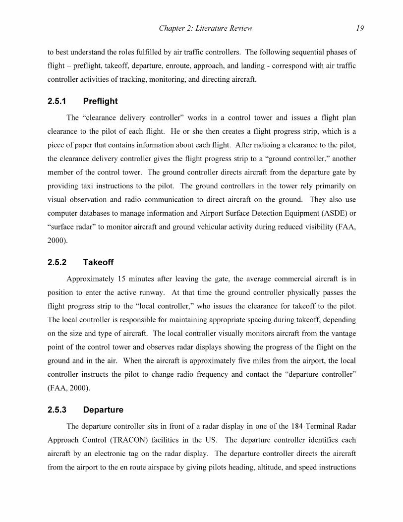
Chapter 2: Literature Review 19
to best understand the roles fulfilled by air traffic controllers. The following sequential phases of
flight – preflight, takeoff, departure, enroute, approach, and landing - correspond with air traffic
controller activities of tracking, monitoring, and directing aircraft.
2.5.1 Preflight
The “clearance delivery controller” works in a control tower and issues a flight plan
clearance to the pilot of each flight. He or she then creates a flight progress strip, which is a
piece of paper that contains information about each flight. After radioing a clearance to the pilot,
the clearance delivery controller gives the flight progress strip to a “ground controller,” another
member of the control tower. The ground controller directs aircraft from the departure gate by
providing taxi instructions to the pilot. The ground controllers in the tower rely primarily on
visual observation and radio communication to direct aircraft on the ground. They also use
computer databases to manage information and Airport Surface Detection Equipment (ASDE) or
“surface radar” to monitor aircraft and ground vehicular activity during reduced visibility (FAA,
2000).
2.5.2 Takeoff
Approximately 15 minutes after leaving the gate, the average commercial aircraft is in
position to enter the active runway. At that time the ground controller physically passes the
flight progress strip to the “local controller,” who issues the clearance for takeoff to the pilot.
The local controller is responsible for maintaining appropriate spacing during takeoff, depending
on the size and type of aircraft. The local controller visually monitors aircraft from the vantage
point of the control tower and observes radar displays showing the progress of the flight on the
ground and in the air. When the aircraft is approximately five miles from the airport, the local
controller instructs the pilot to change radio frequency and contact the “departure controller”
(FAA, 2000).
2.5.3 Departure
The departure controller sits in front of a radar display in one of the 184 Terminal Radar
Approach Control (TRACON) facilities in the US. The departure controller identifies each
aircraft by an electronic tag on the radar display. The departure controller directs the aircraft
from the airport to the en route airspace by giving pilots heading, altitude, and speed instructions

Chapter 2: Literature Review 20
to safely guide each aircraft to its cruise altitude via an air corridor. After directing the aircraft to
a point near the boundary of the TRACON, the departure controller electronically hands-off the
aircraft to a “center controller” at one of the 21 Air Route Traffic Control Centers (ARTCC) in
the US. The departure controller instructs the pilot to change radio frequency and contact the
center controller (FAA, 2000).
2.5.4 Enroute
Center controllers monitor flights on a radar display during the cruise phase by providing
spacing and weather advisories to the pilots. Each center consists of approximately 20 sectors
each monitored by two center controllers. As each flight passes through the center controller’s
sector, he or she hands-off the flights to either another center controller or to a TRACON
“approach controller” if the aircraft needs to descend towards a final destination. Center
controllers use computer based prediction tools, such as the Traffic Management Advisor
(TMA), to determine when congestion may occur at an airport due to too many simultaneous
arrivals. The TMA provides recommended flight adjustments that controllers may issue in order
to adjust aircraft arrivals to remain within the capacity of the airport (FAA, 2000).
2.5.5 Approach
Like the departure controller, the approach controller observes a radar display in the
TRACON. The approach controller simultaneously separates aircraft and sequences them into a
smooth flow of arrivals at the destination airport by instructing pilots to change heading, speed,
and altitude. The approach controller instructs the pilot to change radio frequency to contact the
local controller when the aircraft is approximately 10 miles from the destination airport. In
addition to the radar display, some TRACONs have the Final Approach Spacing Tool (FAST) to
help approach controllers determine how to best sequence arriving aircraft according to their size
and capabilities (FAA, 2000).
2.5.6 Landing
Similar to takeoff, but in the opposite order, the controllers in the tower control the arriving
aircraft from about 10 miles away from the airport until the aircraft parks at a gate. The local
controller issues a landing clearance and directs the aircraft off of the runway onto a taxiway.
The ground controller provides taxi instructions to safely direct the aircraft to an arrival gate.
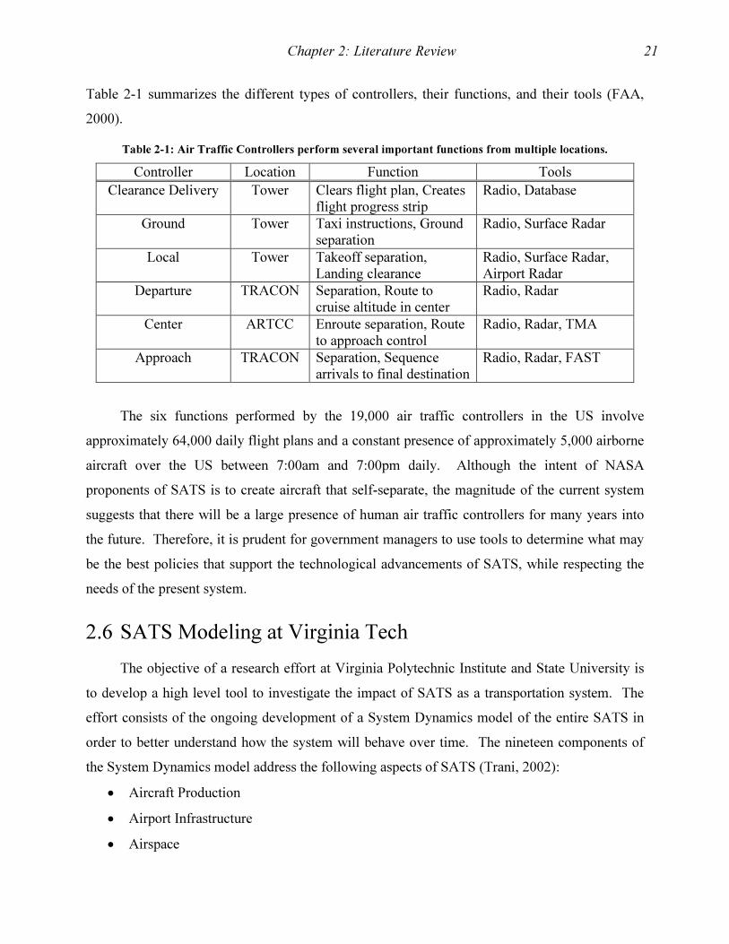
Chapter 2: Literature Review 21
Table 2-1 summarizes the different types of controllers, their functions, and their tools (FAA,
2000).
Table 2-1: Air Traffic Controllers perform several important functions from multiple locations.
Controller Location Function Tools
Clearance Delivery Tower Clears flight plan, Creates flight progress strip
Radio, Database
Ground Tower Taxi instructions, Ground separation
Radio, Surface Radar
Local Tower Takeoff separation, Landing clearance
Radio, Surface Radar, Airport Radar
Departure TRACON Separation, Route to cruise altitude in center
Radio, Radar
Center ARTCC Enroute separation, Route to approach control
Radio, Radar, TMA
Approach TRACON Separation, Sequence arrivals to final destination
Radio, Radar, FAST
The six functions performed by the 19,000 air traffic controllers in the US involve
approximately 64,000 daily flight plans and a constant presence of approximately 5,000 airborne
aircraft over the US between 7:00am and 7:00pm daily. Although the intent of NASA
proponents of SATS is to create aircraft that self-separate, the magnitude of the current system
suggests that there will be a large presence of human air traffic controllers for many years into
the future. Therefore, it is prudent for government managers to use tools to determine what may
be the best policies that support the technological advancements of SATS, while respecting the
needs of the present system.
2.6 SATS Modeling at Virginia Tech
The objective of a research effort at Virginia Polytechnic Institute and State University is
to develop a high level tool to investigate the impact of SATS as a transportation system. The
effort consists of the ongoing development of a System Dynamics model of the entire SATS in
order to better understand how the system will behave over time. The nineteen components of
the System Dynamics model address the following aspects of SATS (Trani, 2002):
• Aircraft Production
• Airport Infrastructure
• Airspace
Chapter 2: Literature Review 22
• Air Traffic Controllers
• Communications
• Economics
• Energy
• Measures of Effectiveness
• Modal Split
• Air Transportation Network Assignment
• Noise
• Pilot Training
• Population
• Safety
• SATS Vehicle Technology
• Service Provider Operations
• Transportation Cost
• Trip Distribution
• Trip Generation
Researchers are making progress in several areas of the above model: trip generation, trip
distribution, noise, and the air transportation network assignment submodels. The other
submodels still require study and refinement. The research effort in this document will relate to
the air traffic controllers submodel.
2.7 The FAA Strategic Decision Support System Model
Also using the System Dynamics approach, developers of a strategic decision support
system for the FAA (Suiter & Peterson, 2001) created a submodel on Air Traffic Control
Capacity that includes three major ATC system constraints: infrastructure, communication
bandwidth, and air traffic control personnel. The developers defined infrastructure as the
combination of radars, computers, buildings, and repair facilities. Their submodel contains
variables to replicate infrastructure details such as budgets, equipment age, and deterioration.
However, the developers considered bandwidth and the number or air traffic controllers as
constants in the system. The rationale for the use of a constant to represent bandwidth is that the

Chapter 2: Literature Review 23
amount available cannot change without the introduction of new technology to use it and
negotiation to obtain it from another user. The rationale for the use of a constant number of air
traffic controllers is that, “Historical trends have shown that the capacity of the system is not
strongly tied to the mere number of air traffic controllers” (Suiter & Peterson, 2001, p. 15). The
developers point out that air traffic controllers were able to surge operations and operate with
greater than normal collaboration during events such as the Gulf War in 1991.
The developers base their claims regarding the capabilities of air traffic control personnel
on interviews made with subject matter experts in the FAA. Many of the interviewees indicated
that controller “ingenuity and ability to adapt as a primary factor in system performance (keeping
out of gridlock)” (Suiter & Peterson, 2001, p. 42). Yet the developers chose to model the
controllers with a constant instead of looking deeper into the role of the controllers to determine
how other variables may account for aspects such as ingenuity and adaptability. Interviewees
also indicated that the National Air Traffic Controllers Association (NATCA) impedes the
introduction of new equipment to aid controllers as a negotiating bargaining chip. Interviewees
pointed out three issues involving controller pay and incentives: first, controller pay is a function
of the volume and complexity of the air traffic they control; second, controller pay lacks
incentives for inter-controller cooperation; and third, current policies dictate individual
punishment for violating rules such as not adhering to minimum aircraft separation standards.
Interviewees claim some controllers act on biases, such as increasing separation distances when
they hear a female pilot’s voice or stubbornly delaying an aircraft to show dominance over a
pilot. Interviewees expressed concern that the high number of controllers taking a summer
vacation caused excessive overtime and understaffing. Although the developers of the ATC
submodel chose not to consider the effects of NATCA, pay, punishment, bias, and vacation
policies, further research into the implications of these issues may improve understanding of the
performance of the air traffic control system.
2.8 European Shortages of Air Traffic Controllers
A study done by Eurocontrol, the European organization for the safety of air navigation,
includes several reasons for a shortage of air traffic controllers in Europe. First, the population
pool from which controllers emanate also provides employees to other competing industries, so
there is a recruiting challenge. Second, the volume of air traffic has increased faster than the

Chapter 2: Literature Review 24
abilities of the controller base. Third, insufficient long-term manpower management has been
weak. It does not adequately take into account changes in the airspace, volume of traffic, new
technology, working conditions, leaves, and administrative job requirements assigned to
controllers. Fourth, planners did not adequately considered early retirement or burnout that
causes controllers to leave the system sooner than they might otherwise. Fifth, although it helps
improve performance and reduce workload, new technology has not yet replaced the need for
human controllers, nor will it do so under current plans for the future. Sixth, there is a 25%
failure rate among new controllers in either initial training or on the job training, and, due to lack
of instructors the controller training capacity operates at 80% of its capability (Skoniezki, 2001).
The US system may face similar problems soon as the majority of controllers currently in the
system began their careers as replacements for the controllers fired in the 1981 strike.
2.9 Preview: A System Dynamics Approach to Air Traffic
Control Manpower and Infrastructure Modeling
The history and anticipated requirements of ATC provide insight into the underlying
causes of the events that influenced the development of ATC capabilities in the past and the
future impacts of demand and modernization upon ATC. Many of the past events and future
conditions that influence ATC are expressible in terms of quantities and equations such as
numbers of aircraft, aircraft performance capabilities, safety records, capital equipment, and
numbers of controllers. The quantities and equations provide the input that is useful for
developing mathematical models of ATC.
A significant portion of the research effort outlined in this document will involve the
search for valid descriptions of the quantities and equations associated with the variables in an
ATC manpower and infrastructure resource management model. Measurements of the activities
in the ATC system in terms of flows of people, aircraft, ATC capital equipment, money, and
information will provide a basis upon which to evaluate how structure, delays, and decision-
making shape system behavior to create stability, growth, or decay (Forrester, 1961). For
example, Figure 2-7 depicts the flow of air traffic controllers through a system involving
training, controlling, and retirement. Expanding the structure of the model may include the
various functions of air traffic control at towers, TRACONS, or centers as well as administrators
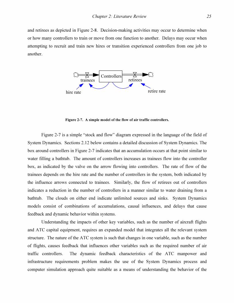
Chapter 2: Literature Review 25
and retirees as depicted in Figure 2-8. Decision-making activities may occur to determine when
or how many controllers to train or move from one function to another. Delays may occur when
attempting to recruit and train new hires or transition experienced controllers from one job to
another.
Controllersretireestrainees
hire rate retire rate
Figure 2-7. A simple model of the flow of air traffic controllers.
Figure 2-7 is a simple “stock and flow” diagram expressed in the language of the field of
System Dynamics. Sections 2.12 below contains a detailed discussion of System Dynamics. The
box around controllers in Figure 2-7 indicates that an accumulation occurs at that point similar to
water filling a bathtub. The amount of controllers increases as trainees flow into the controller
box, as indicated by the valve on the arrow flowing into controllers. The rate of flow of the
trainees depends on the hire rate and the number of controllers in the system, both indicated by
the influence arrows connected to trainees. Similarly, the flow of retirees out of controllers
indicates a reduction in the number of controllers in a manner similar to water draining from a
bathtub. The clouds on either end indicate unlimited sources and sinks. System Dynamics
models consist of combinations of accumulations, causal influences, and delays that cause
feedback and dynamic behavior within systems.
Understanding the impacts of other key variables, such as the number of aircraft flights
and ATC capital equipment, requires an expanded model that integrates all the relevant system
structure. The nature of the ATC system is such that changes in one variable, such as the number
of flights, causes feedback that influences other variables such as the required number of air
traffic controllers. The dynamic feedback characteristics of the ATC manpower and
infrastructure requirements problem makes the use of the System Dynamics process and
computer simulation approach quite suitable as a means of understanding the behavior of the
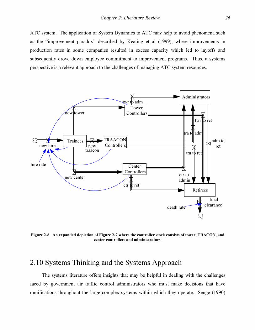
Chapter 2: Literature Review 26
ATC system. The application of System Dynamics to ATC may help to avoid phenomena such
as the “improvement paradox” described by Keating et al (1999), where improvements in
production rates in some companies resulted in excess capacity which led to layoffs and
subsequently drove down employee commitment to improvement programs. Thus, a systems
perspective is a relevant approach to the challenges of managing ATC system resources.
Trainees
Tower
Controllers
TRAACON
Controllers
Center
Controllers
new hires new
traacon
new center
new tower
Administrators
hire rate
Retirees
tra to ret
tra to adm
twr to adm
ctr to ret
ctr to
admin
twr to ret
adm to
ret
final
clearancedeath rate
Figure 2-8. An expanded depiction of Figure 2-7 where the controller stock consists of tower, TRACON, and
center controllers and administrators.
2.10 Systems Thinking and the Systems Approach
The systems literature offers insights that may be helpful in dealing with the challenges
faced by government air traffic control administrators who must make decisions that have
ramifications throughout the large complex systems within which they operate. Senge (1990)
Chapter 2: Literature Review 27
offered systems oriented insights for managers of large complex systems by popularizing the
notion of “systems thinking,” which he defined as “a conceptual framework, a body of
knowledge and the tools that has been developed over the past fifty years…” (p. 7). Senge
intended to shift the mindset that managers controlled isolated organizations to the mindset that
many interrelated forces influenced organizational behavior. He advocated the use of systems
thinking as the foundation upon which managers could create a “learning organization – an
organization that is continually expanding its capacity to create its future” (p. 14), by designing
structure into organizations to shape growth, thinking, and communication. Senge’s approach
sets the stage for the search to identify and understand the concepts, knowledge, and tools of
systems thinking that may help managers of complex organizations improve their decision-
making abilities.
Blanchard and Fabrycky (1998) address the basic concepts of systems thinking by
defining a system as “a set of interrelated components working together toward some common
objective or purpose” (p. 2). They claim that the world is transitioning from thinking dominated
by reductionism and mechanism to a new thinking dominated by expansionism. Reductionism
breaks things down into small pieces; mechanism assigns a specific cause to each event.
Expansionism attributes behavior to the interrelationships of many parts. The significance of the
transition in human thinking from breaking things down to putting things together is twofold.
First, people recognize that they can combine the three concepts of reductionism, mechanism,
and expansionism by focusing on how the interrelationships of many parts influence the behavior
of the whole. Second, people realize that trying to make each part perform optimally often
causes the system to perform less than optimally. Blanchard and Fabrycky describe the new
thinking as the “systems approach” (p. 12).
Churchman (1968), a pioneering systems thinker in the 1960s, described the systems
approach as “simply a way of thinking about these total systems and their components” (1968, p.
11). He claimed “every system is embedded in a larger system” (p. 48) and presented the idea
that the “larger system” may actually be the world in the future - thus connecting the aspect of
time with systems thinking. He alluded to the direct relationship between structure and behavior
by stating; “The management scientist sees the nature of the whole system as a determinant of
individual behavior” (p.200). Although Churchman believed few managers understood how they
determined what important variables to monitor in their systems, he believed it was possible to

Chapter 2: Literature Review 28
provide managers with a systems approach that would help them understand what to attend to
and why.
Churchman advocated a scientifically oriented systems approach centered on the use of
mathematical or behavioral models to describe systems. He defined a model as “a way in which
the human thought process can be amplified” (p. 61). He believed that modelers should consider
five aspects of systems: 1) the objective of the system and system performance metrics; 2) the
environment of the system – those things which effect the system but which the system cannot
influence very much; 3) the resources inside the system that it uses to accomplish the objective;
4) the system’s components, their activities and performance; and 5) the management of the
system. Churchman recognized that one would truly know they were viewing the system as a
whole when they could see the system intentionally sacrifice lesser goals in the pursuit of it’s
true objective. Such an approach was somewhat radical in its time and still may prove
challenging for government managers battling among each other for constrained resources. The
approach would require one agency or department to intentionally shortchange its own efforts in
order to provide another agency or department with the resources that increase the performance
of the larger system.
To operate at such a challenging, benevolent, and sacrificial level of thinking, Richmond
(1993) proposed seven “systems thinking skills” that individuals should develop separately and
use simultaneously in order to be effective systems thinkers. He recommended learning the
following skills separately in order to prevent the “cognitive overload” experienced by people
trying to learn them all at once:
1. Dynamic thinking: the ability to focus on patterns of behavior over time rather than on
specific events.
2. Closed-loop Thinking: observing a system as an interdependent spider web of
components rather than as an organizational chart of singular cause and effect
relationships.
3. Generic thinking: attributing events to the structure of the system, not to specific
individuals.
4. Structural thinking: recognizing and appreciating the dimensions of the stocks and flows
in a system. Note: section 2.12.1 below contains definitions of stocks and flows.
Chapter 2: Literature Review 29
5. Operational thinking: realistically integrating the essential elements required to make a
system operate.
6. Continuum thinking: replacing the polarizing if-then-else approach to decision-making
with acceptance of multiple possibilities along a continuum of alternatives.
7. Scientific thinking: quantifying variables and using them to test hypotheses.
The above skills provide not only a framework for understanding system thinking, but also
recognition of the depth and diversity of thought and talent required to address the dynamic
nature of problems within systems. Clearly, an effective systems approach involves
thoroughness, openness, and the abilities to research and communicate. As O’Connor &
McDermott (1997) see it, “Systems thinking is the way we can discern some rules, some sense of
patterns and events, so we can prepare for the future and gain some influence over it” (p. xiv).
The concepts and frameworks by Senge, Blanchard & Fabrycky, Churchman, Richmond
and O’Connor & McDermontt provide a foundation for the application of systems thinking
toward the challenges of managing manpower and infrastructure in the US ATC system. In
particular, the above perspectives allude to or directly advocate the usage of the tools and
procedures associated with the computer modeling of the System Dynamics process. They
advocate the sort of systems thinking that goes beyond observing, thinking, diagramming and
talking about systems. Forrester cautioned that such superficial systems thinking (Forrester,
1994) lacks the rigor of the “quantitative and dynamic analysis that constitutes real System
Dynamics” (Koegh & Doman, 1992, p. 10), which leads people to an understanding of how
management policies shape decision-making within a system. A further investigation of the
concepts, processes, and tools of System Dynamics will clarify how researchers may apply it to
increase understanding of the dynamic interactions among air traffic controllers, flights, capital
equipment, and other resources in order to determine the potential behavior of the ATC system
under various resource management scenarios and with the introduction of SATS aircraft into the
system.
2.11 System Dynamics
Coyle (1996) defines System Dynamics as a qualitative and quantitative approach to
describe, model, and design structure for managed systems in order to understand how delays,
feedback, and interrelationships among variables influence the behavior of the system over time.

Chapter 2: Literature Review 30
Coyle claims that managers can use System Dynamics to model the effects of manipulating
policies governing the system in order to create more desired system behavior. Sterman (2000,
1994) describes System Dynamics as an aid to learning and understanding complex systems. He
emphasizes how the System Dynamics modeling process consists of tools to elicit mental models
of systems, procedures to create formal models based on the mental models, computer
simulations of the formal models, and applications of the findings of the simulations to improve
understanding of the system. Lyneis (1999) highlights the business application of System
Dynamics as an approach that combines a client’s decision-making processes and computer
simulation models to develop decision-making tools. The definition from the System Dynamics
Society website defines System Dynamics as “a methodology for studying and managing
complex feedback systems” (System Dynamics Society, 2001). Mathematically, System
Dynamics models consist of nonlinear ordinary differential equations (Sterman, 2000). The
fundamental insights from the above definitions of some of the leading researchers and
practitioners in the field of System Dynamics are:
� System Dynamics is qualitative and quantitative.
� System Dynamics is a process involving elicitation, modeling, and simulation
tools.
� System Dynamics is useful as a learning process and a means to create tools to aid
understanding.
� System Dynamics describes systems in terms of interactions with delays and
feedback.
The System Dynamics concepts listed above provide a framework for researchers who seek to
understand complex systems. The System Dynamics approach will be useful to investigate the
impact of SATS upon the complex NAS.
The roots of Coyle and Sterman’s descriptions of System Dynamics lie in Forrester’s
seminal work that originally introduced the concept of System Dynamics, initially with the term
“industrial dynamics.” Forrester (1961) claimed in his preface to Industrial Dynamics that,
“Industrial dynamics is a way of studying the behavior of industrial systems to show how
policies, decisions, structure, and delays are interrelated to influence growth and stability. It
integrates the separate functional areas of management – marketing, investment, research,
personnel, production, and accounting. Each of these functions is reduced to a common basis by
Chapter 2: Literature Review 31
recognizing that any economic or corporate activity consists of flows of money, orders,
materials, personnel, and capital equipment” (p. vii). Since Forrester conducted his initial work,
researchers have applied System Dynamics to a variety of business, medical, environmental,
economic, military, and social issues. The approach appears well suited for the ATC resource
management and SATS/NAS integration issues as the system consists of functional areas and
flows of personnel (air traffic controllers), investment (government appropriations), production
(flights), accounting (performance measures), capital equipment (radar or satellite navigation
systems), and material (aircraft) in the system.
2.12 System Dynamics Terminology and Tools
The System Dynamics literature is replete with descriptions of concepts and tools useful
for modeling. However, the still maturing field does not have a formal standard of definitions.
Subsequently, practitioners and theorists offer their descriptions of terms in their work. There is
much commonality, yet there is also diversity of opinion, in cases such as the use of system
archetypes. The following definitions incorporate the perspectives of several leaders in the field
of System Dynamics, such as Forrester, Sterman, Ford, Coyle, Senge, and others. In general
their views reflect the fundamental concept of System Dynamics that feedback structures of
interconnected stocks and flows govern system behavior (Forrester,1961; Coyle, 1996; Ford,
1999; Sterman, 2000). Thus, the definitions and tools below relate to those aspects of system
behavior.
2.12.1 Fundamental Concepts of System Dynamics
Stock: Stocks are the most important variables in a model. Stocks represent accumulations of
some measurable entity (Ford, 1999). According to Sterman (2000), stocks “characterize the
state of the system and generate the information upon which decisions and actions are based” (p.
192). Stocks may be people, parts, money, or even intangibles such as happiness. In Figure 2-7,
the box around “controllers” identifies it as a stock. Table 2-2 provides a variety of
interpretations of stocks under the heading “accumulation.”
Flow: Flows are the physical or conceptual entities in systems that move over time. Examples of
flows include people, material, or subjective concepts such as satisfaction. Flows into or out of
stocks cause them to change. Sources and sinks are infinite capacities from which flows may

Chapter 2: Literature Review 32
originate or into which flows may depart. In Figure 2-7, the valve symbol above “trainees”
identifies it as a flow. Table 2-2 provides a variety of interpretations of flows under the heading
“action.”
Auxiliaries: Sterman (2000) describes auxiliary variables as “intermediate concepts added to the
model to aid clarity” (p. 205). Similarly, Coyle (1996) describes auxiliaries as “intermediate
stages by which the levels determine the rates” (p. 86). Ford (1999) also claims that they help to
“describe the flow” (p. 19) and serve as a tool to calculate system performance metrics. In
Figure 2-7, “hire rate” is an auxiliary variable. Table 2-2 provides a variety of interpretations of
auxiliary variables under the heading “auxiliary.”
Table 2-2: Many different terms describe the concepts of stocks, flows, and auxiliary variables.
Source Accumulation Action Auxiliary
Forrester Levels Rates Multiplier
Sterman (2000) Stock Flow Auxiliary
Ford (1999) Stock Flow Converter
Mathematics Integration Differentiation Parameter
Grammatical Analogue Noun Verb Adverb
Assembly line Buffer Machine and Conveyor throughput
Machine and conveyor speed
Bank Analogy Bank Account Balance
Interest added Interest rate
Bounded Rationality: The concept that the unaided human mind cannot intuitively solve
dynamically complex problems. From his studies of people working with simulations, Sterman
(2000) believes people “misperceive feedback” because “the mental models people use to guide
their decisions are dynamically deficient” (p. 27). System Dynamics is a tool to overcome the
normal responses to bounded rationality, such as habits or rules of thumb (Sterman, 2000).
Delay: Stocks create delays in a system when the flow into the stock is greater than the flow out
of the stock (Sterman, 2000).
Detail Complexity: Systems or decision-making situations characterized by many components
or alternatives from which to choose have detail complexity due to the large numbers of
combinations they present (Sterman, 2000).
Chapter 2: Literature Review 33
Dynamic Complexity: Dynamic complexity occurs in systems characterized by large numbers
of interactions over time where feedback and delays make it impossible to intuitively determine
the behavior of even simply structured systems (Sterman, 2000).
Endogenous variables: Model variables that lie within the boundary of a model where the
structure and policies within the modeled system influence the variables’ behavior (Sterman,
2000).
Exogenous variables: Variables outside the model boundary that have no causal connection
from the endogenous variables within the model boundary, but have causal connections to the
endogenous variables in the model. Ideally, exogenous variables remain constant throughout the
time horizon of the model (Sterman, 2000; Ford, 1999).
Feedback: Feedback occurs in a system when its own past activity influences its future.
Negative feedback in a system causes the system to seek a goal such as when a thermostat starts
and stops heating and cooling systems. In System Dynamics models, negative feedback loops
are called balancing loops. Positive feedback generates continuous growth or decay, such as
when a bank account accrues compound interest. In System Dynamics models, positive
feedback loops are called reinforcing loops (Forrester, 1971; Sterman, 2000).
Graphical System Behavior: Graphs of the behavior of key variables in a system are an
important product of System Dynamics models. Typical patterns on System Dynamics graphs
show growth, decay, goal setting, and oscillation.
Intended Rationality: The concept that people make decisions according to their mental model
of the outcome of their decisions within their perceived environment. The challenge for System
Dynamics modelers is to represent the decision-making, the mental models, and the environment
in a computer model of a system (Sterman, 2000).
Level of Aggregation: Sterman (2000) claims that most clients desire at least twice as much
detail in a System Dynamics model than is needed to appreciate system behavior, however, client
satisfaction requires the modeler to include enough detail to make the client use the model as a
basis for action. Modelers should keep in mind the purpose of the model and seek to aggregate
those parts of the system that occur close enough in time, accumulate in similar stocks, or reside
in stocks for a similar amount of time.
Mental models: Senge et al (1994) describes mental models as “internal pictures of the world”
(p. 6). Doyle and Ford (1998) found that definitions of “mental models” varied greatly within

Chapter 2: Literature Review 34
System Dynamics and among practitioners in other fields. Therefore, Doyle and Ford proposed
a definition for “mental models of dynamic systems” (p. 17) as a long lasting, easily recallable,
and generally accurate cognitive structure of a system.
Model boundary: The line separating endogenous variables from exogenous variables. All
components within the boundary of the model, such as stocks, flows, and auxiliary variables, are
influenced by the policies and structure governing the system (Sterman, 2000; Ford, 1999).
Policy: The rules that govern organizational strategy, organizational structure, and how and
when decisions should be made in an organization. Modelers use System Dynamics models to
evaluate how changes to policies and interactions among policies affect system behavior over
time (Sterman, 2000). According to Coyle (1996), policies consist of structure, represented by
descriptive equations and causal links, and parameters, represented by adjustable quantities in a
system. Maani and Cavana (2000) describe policies as individual variables or specific structural
relationships among variables.
Social System: According to Forrester (1998), “The idea of a social system implies that the
relationship between its parts strongly influence human behavior” (p.1). Examples of social
systems include organizations, communities, and teams. Social systems influence peoples’
behavior because they respond to the circumstances created by the structure and feedback of the
system.
System: Blanchard and Fabrycky (1998) define a system as “a set of interrelated components
working together toward some common objective or purpose” (p. 2). Similarly, Forrester (1971)
defines a system as “a grouping of parts that operate together for a common purpose” (p.1-1).
Systems thinking: The mindset that many interrelated forces influence organizational behavior
(Senge, 1990) coupled with the abilities to focus on patterns of behavior over time, to see how
system structure influences behavior, to think in terms of stocks and flows, and to accept
multiple possibilities along a continuum of alternatives (Richmond, 1993).
Units: It is important to maintain unit integrity throughout a System Dynamics model. Ford
(1999) points out that the units of a flow variable are the same as the stock it flows into or out of
divided by time.
Chapter 2: Literature Review 35
2.12.2 System Dynamics Modeling Tools
Boundary Chart: A listing of endogenous, exogenous, and excluded variables of a model that
define the domain of the problem to which the model applies (Sterman, 2000). Ford (1999) uses
a “bull’s-eye diagram” to communicate the same concept and information.
Causal Loop Diagram: A picture of the endogenous and exogenous variables in a system
connected by arrows that depict cause and effect relationships among them in order to illuminate
the feedback structure, or feedback loops of the system (Sterman, 2000; Ford, 1999). Causal
loop diagrams are also know as “influence diagrams.”
Dynamic Hypothesis: Sterman defines a dynamic hypothesis as “a working theory of how the
problem arose” (2000, p. 95) in terms of stocks, flows, and feedback. Ford (1999) describes the
initial System Dynamics model as the “dynamic hypothesis for the system behavior” (p. 172).
Thus, the dynamic hypothesis is a modeler’s early conjecture, which usually evolves through the
System Dynamics modeling process, of how a problem arose from the structure and relationships
among the components of a system.
Equilibrium diagrams: Equilibrium occurs in a model when the inflow and outflow from each
stock are equal. Ford (1999) creates an equilibrium diagram by writing the value and units of
each variable on a stock and flow diagram. He uses equilibrium diagrams to highlight potential
inconsistencies in a model, illuminate incorrect use of units, and set the conditions to determine
the relative stability of the system.
Partial Model Test: The action of isolating a portion of a model where decision-making occurs
to ensure that the decision making process reflects the mental model of the decision-maker by
changing exogenous inputs and observing the behavior of the isolated system. The partial model
test allows modelers to ensure the model captures people’s intended rationality (Sterman, 2000).
Policy Structure Diagram: Maps of the information streams that prompt managers to make
decisions to adjust the rates of flow of the endogenous variables they can control (Sterman,
2000).
Proxy variable: A proxy variable is a variable in a model that takes the place of a variable or
condition that is too complex to replicate in a computer model. For example, in a System
Dynamics model of Mono Lake in California, Ford (1999) uses the variable “elevation” of the
surface of a lake as a proxy for the state of the lake’s ecosystem, which is difficult to model, but
corresponds closely with the elevation of the surface of the lake.

Chapter 2: Literature Review 36
Reference modes: Ford (1999) describes reference modes as a modeler’s initial expectation of
how the model will graphically depict the behavior of a selected variable in the system being
modeled. The modeler draws the reference mode based on expected growth, decay, or
oscillation. The horizontal axis represents the time period under consideration and the vertical
axis represents the particular variable being modeled. The shape of the reference mode is
relative to the vertical axis, yet does not have exact values as the structure of the model should
reproduce the shape, while the parameter values move the shape relative to the range of values
on the axes. Sterman (2000) describes reference modes as sets of graphs that show how a
problem evolved in the past and how it may go forward into the future. Modelers also identify
key variables and their time horizons while developing reference modes. Figure 1-1 is an
example of a reference mode. Reference modes often reflect patterns of growth, decay, goal
seeking, or oscillation.
Stock and Flow Diagram: A depiction of the physical configuration of the system and the
relationships among system variables (Sterman, 2000). Figure 2-7 and Figure 2-8 are examples
of stock and flow diagrams.
Subsystem Diagram: A high-level overview or a series of hierarchical views of the system and
problem the modeler will address (Sterman, 2000). Subsystem diagrams depict the general
structure, flows, and interconnections among the major components of a system.
System Archetypes: Senge (1990) describes “system archetypes” as common structures that
create consistent patterns of behavior in a wide range of systems in fields as diverse as biology,
psychology, politics, economics, and management. He claims that archetypes are useful to
identify where to influence systems in order to change behavior.
Time Horizon: Sterman (2000) describes the time horizon as the span of time that includes the
period when a problem emerged and the future impact of alternative policies. The time horizon
is the horizontal axis of a reference mode graph. Sterman cautions modelers to select a
sufficiently long time horizon to capture the effects of delays. He recommends establishing a
time horizon “several times” (p. 94) longer than the biggest delay in the system. If large
oscillations are present, Ford (1999) advocates a time horizon long enough to see “two or three
oscillations” (p. 172) to determine if they dampen.
Time step: Ford (1999) offers a rule of thumb for setting the time delta or time step in a
simulation; set the DT to less than half of the smallest time constant in the model. He also
Chapter 2: Literature Review 37
recommends keeping simulations under 1000 time step iterations when running the model by
using an appropriate DT and a reasonable time horizon. Sterman (2000) makes several
recommendations regarding the time step in a model. First, he recommends setting the time step
“between one-fourth and one-tenth the size of the smallest time constant in your model” (p. 907).
Second, he recommends checking the time step by cutting it in half until the model is no longer
sensitive to the size of the time step. Third, he recommends selecting a base-2 time step, such as
4, 2, 1, 0.5, 0.25, 0.125, to minimize rounding error caused by truncation of numbers in a
computer, which uses the binary system. Fourth, when mixing years and months between the
model and historical data, he recommends expressing 1/12 with as many digits as possible
(0.833333…), or use months as the time step and divide all numbers expressed in years by
twelve.
2.13 Why Use System Dynamics
Sterman (1994) advocates the use of System Dynamics because managers, decision-
makers, and citizens in general do not have sufficient time to learn from feedback in the form of
outcomes within the systems in which they operate over the natural course of time. The delays
between action and feedback are too long to allow for timely learning or the maturation of
decision-rules. Due to “bounded rationality,” Sterman (2000) claims that the unaided human
mind is unable to cognitively map and process the dynamic relationships within systems of
complex causal relationships. The history of air traffic control, characterized by delays in the
implementation of systems and by feedback in the form of accidents or controller strikes,
supports Sterman’s perspective that the natural learning process is too long and too complex for
the human mind to comprehend.
Ford (1999) uses System Dynamics to create clear, simple models of environmental
systems; such as reservoir water levels, deer herds, or global warming because the approach
emphasizes the type of feedback and nonlinear relationships that are prevalent in natural systems.
He sites four views of equilibrium in natural systems, shown in Figure 2-9, and claims that the
“homeostatic plateau” (Odum, 1971) depicted in the lower right shows the concept of a “span of
control” within which a perturbed system will return to equilibrium, up to a point. If pushed too
far beyond the span of control, the forces creating positive feedback in such a system will
become dominant and change the fundamental nature of the system. He advocates the use of

Chapter 2: Literature Review 38
System Dynamics for both analysis of the stability of systems and for training managers to better
understand the potential behavior of systems. Ford’s natural environment perspective for
training and analysis, applied to the air traffic control system, may shed light on the effects of
events such as the terrorist attacks of September 11, 2001, by providing natural analogues to the
extremes of observed and modeled system behavior.
Figure 2-9. Four views of equilibrium (Ford, 1999).
From a practical business perspective, Lyneis (2000) recommends the use of System
Dynamics models to “forecast” the behavior of markets. He claims that the structural orientation
of System Dynamics models provides more accurate depictions of short and mid-term behavior
than statistical models, which often become skewed by “noise” in the system. He claims that the
use of System Dynamics models not only aids decision-making, but also identifies what
variables in a system have the greatest impact on decision-making and deserve the most attention
over time. In the domain of air traffic control, Lyneis’ market perspective of System Dynamics
makes it a useful tool for administrators responsible for making resource allocation decisions
based on their interpretation of the past and present behavior of the system. As an alternative
approach, System Dynamics offers a more comprehensive and rigorous view of a system than
the inadequate mental models usually used by decision-makers. System Dynamics tools can help
government air traffic control resource managers identify key variables to monitor, such as the
number of aircraft registered in the US or the average age of capital equipment, and then forecast
stable unstable
neutral homeostatic
plateau
Chapter 2: Literature Review 39
potential system behavior based on manipulations of the key variables or other variables related
to them.
Over the past forty years, Forrester described a number of reasons to use the System
Dynamics approach. In his seminal work, Forrester (1961) claimed that management was
transitioning from an art to a science, thus allowing the approach to management based on
principle rather than just experience. Forrester advocated the principle of viewing an
organization as an information-feedback system. Accordingly, he developed the concept of
“industrial dynamics,” the precursor to System Dynamics, to create organizational models that
showed how the structure, policies, decisions, and delays in organizational systems influenced
the growth and stability of the organization. In the early 1990s he advocated the use of System
Dynamics as a tool for CEOs to design their organizations (Koegh & Doman, 1992). He claimed
that CEOs should reduce their participation in operations and instead undertake the role of
designer who determines the structure of the organization, the flow of information, and the
policies governing where decision-making occurs and who makes the decisions. He claimed that
there was an abundance of “information pollution” in organizations that diverted limited
managerial time away from the important information that managers needed to make decisions.
In the late 1990s, Forrester reflected on the usefulness of System Dynamics as an alternative to
designing an organization by “committee and intuition” (1998). He emphasized decisions as
present moment actions, policies as guides to decision-making, and System Dynamics as a
means of determining organizational policy to experiment with alternatives in order to elicit the
desired organizational behavior.
2.14 The System Dynamics Modeling Process
Forrester (1994) acknowledged both the growing interest in System Dynamics and the lack
of guidance for developing System Dynamics simulation models. He described a six-step
System Dynamics process depicted in Figure 2-10. Currently available System Dynamics
software, such as Stella or Vensim, makes it possible for modelers to transition smoothly through
the mechanical aspects of diagramming and equation writing in steps one, two, and three. The
software serves as a tool for modelers to 1) visually describe the system through computerized
stock and flow diagrams, 2) embed equations while building the model, and 3) rapidly simulate
system behavior. Nevertheless, the feedback arrows in Figure 2-10 indicate that Forrester’s
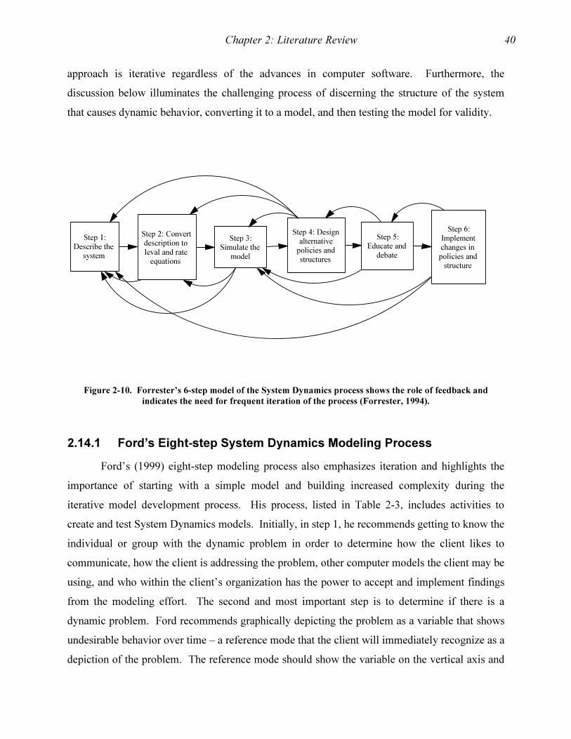
Chapter 2: Literature Review 40
approach is iterative regardless of the advances in computer software. Furthermore, the
discussion below illuminates the challenging process of discerning the structure of the system
that causes dynamic behavior, converting it to a model, and then testing the model for validity.
Figure 2-10. Forrester’s 6-step model of the System Dynamics process shows the role of feedback and
indicates the need for frequent iteration of the process (Forrester, 1994).
2.14.1 Ford’s Eight-step System Dynamics Modeling Process
Ford’s (1999) eight-step modeling process also emphasizes iteration and highlights the
importance of starting with a simple model and building increased complexity during the
iterative model development process. His process, listed in Table 2-3, includes activities to
create and test System Dynamics models. Initially, in step 1, he recommends getting to know the
individual or group with the dynamic problem in order to determine how the client likes to
communicate, how the client is addressing the problem, other computer models the client may be
using, and who within the client’s organization has the power to accept and implement findings
from the modeling effort. The second and most important step is to determine if there is a
dynamic problem. Ford recommends graphically depicting the problem as a variable that shows
undesirable behavior over time – a reference mode that the client will immediately recognize as a
depiction of the problem. The reference mode should show the variable on the vertical axis and
Step 1:
Describe thesystem
Step 2: Convertdescription to
leval and rateequations
Step 3:Simulate the
model
Step 4: Designalternative
policies and
structures
Step 5:Educate and
debate
Step 6:
Implementchanges in
policies andstructure
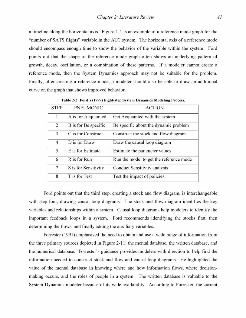
Chapter 2: Literature Review 41
a timeline along the horizontal axis. Figure 1-1 is an example of a reference mode graph for the
“number of SATS flights” variable in the ATC system. The horizontal axis of a reference mode
should encompass enough time to show the behavior of the variable within the system. Ford
points out that the shape of the reference mode graph often shows an underlying pattern of
growth, decay, oscillation, or a combination of these patterns. If a modeler cannot create a
reference mode, then the System Dynamics approach may not be suitable for the problem.
Finally, after creating a reference mode, a modeler should also be able to draw an additional
curve on the graph that shows improved behavior.
Table 2-3: Ford’s (1999) Eight-step System Dynamics Modeling Process.
STEP PNEUMONIC ACTION
1 A is for Acquainted Get Acquainted with the system
2 B is for Be specific Be specific about the dynamic problem
3 C is for Construct Construct the stock and flow diagram
4 D is for Draw Draw the causal loop diagram
5 E is for Estimate Estimate the parameter values
6 R is for Run Run the model to get the reference mode
7 S is for Sensitivity Conduct Sensitivity analysis
8 T is for Test Test the impact of policies
Ford points out that the third step, creating a stock and flow diagram, is interchangeable
with step four, drawing causal loop diagrams. The stock and flow diagram identifies the key
variables and relationships within a system. Causal loop diagrams help modelers to identify the
important feedback loops in a system. Ford recommends identifying the stocks first, then
determining the flows, and finally adding the auxiliary variables.
Forrester (1991) emphasized the need to obtain and use a wide range of information from
the three primary sources depicted in Figure 2-11: the mental database, the written database, and
the numerical database. Forrester’s guidance provides modelers with direction to help find the
information needed to construct stock and flow and causal loop diagrams. He highlighted the
value of the mental database in knowing where and how information flows, where decision-
making occurs, and the roles of people in a system. The written database is valuable to the
System Dynamics modeler because of its wide availability. According to Forrester, the current
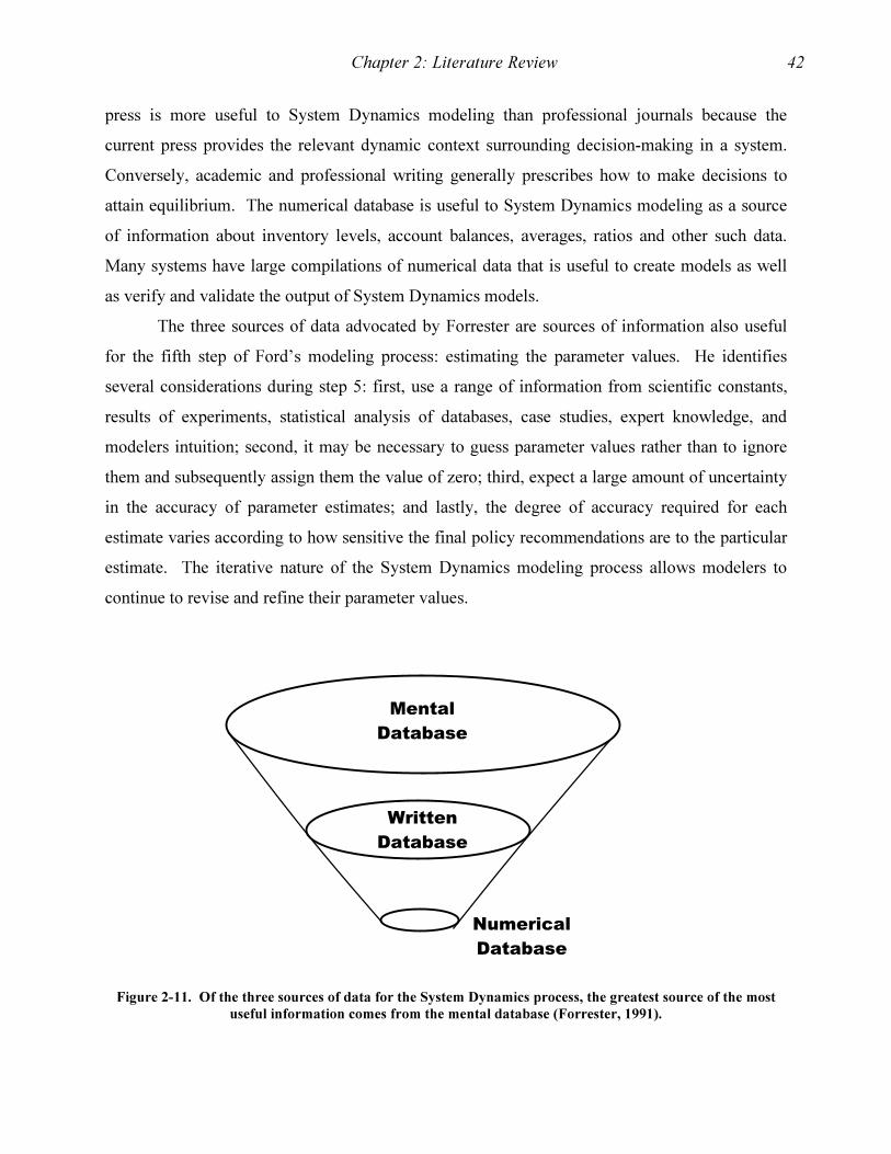
Chapter 2: Literature Review 42
press is more useful to System Dynamics modeling than professional journals because the
current press provides the relevant dynamic context surrounding decision-making in a system.
Conversely, academic and professional writing generally prescribes how to make decisions to
attain equilibrium. The numerical database is useful to System Dynamics modeling as a source
of information about inventory levels, account balances, averages, ratios and other such data.
Many systems have large compilations of numerical data that is useful to create models as well
as verify and validate the output of System Dynamics models.
The three sources of data advocated by Forrester are sources of information also useful
for the fifth step of Ford’s modeling process: estimating the parameter values. He identifies
several considerations during step 5: first, use a range of information from scientific constants,
results of experiments, statistical analysis of databases, case studies, expert knowledge, and
modelers intuition; second, it may be necessary to guess parameter values rather than to ignore
them and subsequently assign them the value of zero; third, expect a large amount of uncertainty
in the accuracy of parameter estimates; and lastly, the degree of accuracy required for each
estimate varies according to how sensitive the final policy recommendations are to the particular
estimate. The iterative nature of the System Dynamics modeling process allows modelers to
continue to revise and refine their parameter values.
Figure 2-11. Of the three sources of data for the System Dynamics process, the greatest source of the most
useful information comes from the mental database (Forrester, 1991).
Mental
Database
Written
Database
Numerical
Database
Chapter 2: Literature Review 43
An important determinant of the need to iterate occurs at Ford’s sixth step: running the
model. If the simulation appears to represent the anticipated pattern recorded in the reference
mode, then the modeler should move on to step 7. Otherwise, the modeler should return to steps
1-3 to gain better understanding of the system, rethink the reference mode diagram, or
reconstruct the stock and flow diagram. Ford’s seventh step, conduct sensitivity analysis,
involves formal or informal tests of the parameters of the model across their full ranges. The
objective of step 7 is to ensure that the underlying feedback structure creates model behavior;
parameter values should not be the driving force behind model behavior. The modeler should
return to step 5 to reconsider parameter estimation if the model behavior pattern changes as
individual parameters vary.
Campbell (2001) described the lessons she learned at Hewlett-Packard while facilitating a
System Dynamics modeling process through the equivalent of Ford’s first six steps. Campbell
recognized the importance of initially accepting detail complexity in her team’s System
Dynamics model in order to develop a sense of ownership and understanding among the model
development team. Contributors to the model initially expected it to reflect their detailed
understanding of system processes. Eventually, during the team and model maturation process,
the detail complexity would give way to a higher-level model with appropriate dynamic
complexity. Campbell described an unexpected, frustrating, but necessary period of confusion
among the model development team as the members transitioned through a period of realigning
their mental models of the system with the behavior depicted by the System Dynamics model of
the system. Campbell played a key role by reassuring her clients that the challenging transition
was a normal part of the process. Finally, she highlighted the value to the client of two other
aspects of the System Dynamics modeling process: first, the development of a common language
of describing systems with influence diagrams and stock and flow diagrams, and second, the
compilation of model data into a single document. Campbell’s insight provides a realistic
perspective on the modeling process that enhances understanding of the process flows advocated
above by Forrester and Ford.
Ford’s final step is to test the various policy options managers may pursue by changing
the values of model variables they can control through policy adjustments. Once a desired policy
emerges, Ford recommends several more actions: first, conduct a sensitivity test of the values of
Chapter 2: Literature Review 44
the parameters managers cannot control while using the values associated with the new policy
variables that the managers can control; second, introduce randomness into the system and
observe the effects; and lastly, consider revising the stock and flow diagram from step 3 to
include more detail in the new policy model.
2.14.2 Sterman’s Five-step System Dynamics Modeling Process
Like Ford, Sterman (2000) offers a detailed description of the System Dynamics
modeling process; he reinforces many of Ford’s perspectives and he offers his own insights.
Sterman points out that modeling is a creative process in which each modeler approaches a
problem differently. However, Sterman claims that there are five essential steps to modeling that
are characteristics of all successful modeling efforts. Table 2-4 lists the five steps and includes
activities and tools used in each step. Supporting Ford’s claim that modeling is an iterative
process, Sterman states that the modeler gets feedback from the real world, adjusts the model,
and then provides additional model feedback to the real world. Sterman also agrees with Ford
that defining the problem is the most important step in the process. Sterman emphasizes the
need to ensure that the purpose of the model is to solve a problem, not simply to model a system.
The model must simplify the system to a point where the model replicates a specific problem.
Sterman advises modelers to be aware of clients who seek validation of their preconceived
notions about system behavior. If the model claims otherwise, then the modeler should
challenge the client’s point of view, stand firmly on the side of truth, and maintain the
responsibility to be ethical and forthright. Otherwise, the modeler should move on to another
problem and another client.
Table 2-4: Sterman’s (2000) Five-step System Dynamics Modeling Process.
STEP ACTION ACTIVITIES
1 Problem Articulation
Define what the problem is and why it is a problem, identify key variables, determine the time horizon, and develop reference modes.
2 Formulation of Dynamic Hypothesis
Develop a dynamic hypothesis that describes the problem as a result of the relationship among the variables and internal structure of the system. Use mapping techniques such as model boundary diagrams, subsystem diagrams, causal loop diagrams, stock and flow diagrams, and policy structure diagrams.
3 Formulation of a Simulation Model
Create a computer model by specifying units, relationships, and equations. Clarify concepts from steps 1 and 2.

Chapter 2: Literature Review 45
4 Testing Check the usefulness of the model by using reference modes, extreme values, sensitivity testing, integration error testing, behavior reproduction testing, behavior anomaly testing, surprise behavior testing, and system improvement testing. Return to previous steps as needed to refine the model.
5 Policy Design and Evaluation
Identify situations and policies to conduct “what if” analysis, then determine the sensitivity and interactions of policies.
Sterman’s second step involves the process of determining what caused the problem by
focusing on structures within the system. The dynamic hypothesis emerges from the process of
selecting primarily endogenous variables, conservatively including few exogenous variables, and
using mapping tools to determine the structure of the relationships among the variables. The
model boundary chart helps modelers to categorize variables as endogenous, exogenous, or
excluded, and, the chart also limits the purpose of the model by defining the boundary of its
domain. Ford (1999) uses a “bull’s-eye diagram” (p. 97) to visually depict the elements of a
boundary diagram. Subsystem diagrams provide an overview of the system architecture within
the domain of the problem under investigation. Causal loop diagrams capture the feedback loops
within the system while stock and flow diagrams provide a description of the structure of the
system. Policy structure diagrams highlight how information prompts decision-making within a
system (Sterman, 2000). Sterman’s emphasis on diagramming tools helps modelers to portray
the problem within a structured system comprised of essential interrelated components, while
capturing the flow of people, material, and information, and at the same time recognizing the
influence of other key elements inside and outside of the system.
In steps three and four of the System Dynamics modeling process, Sterman creates an
operational model that includes “equations, parameters, and initial conditions” (2000, p. 103) and
then tests it. The creation of the first formal computer model requires the modeler to conform to
the unforgiving specificity of the computer. The computer software forces the modeler to clearly
state units, equations, and relationships. In the testing phase, the modeler must ensure that the
model has “dimensional consistency” – the relationships among the units in the stocks, flows,
and auxiliary variables and constants must make sense. The modeler also seeks correlation
between the model and the real world system. Furthermore, modelers should test the model with
extreme values to ensure the behavior of the model conforms to physical laws, such as not
creating a negative population. Several other tests to determine the utility of the model include
Chapter 2: Literature Review 46
sensitivity testing, integration error testing, behavior reproduction testing, behavior anomaly
testing, surprise behavior testing, and system improvement testing.
Sterman (2000) advocates thorough and continuous testing to build confidence in the
model and gain insight into the system. He encourages modelers to ensure that the model
conforms to the original purpose of the modeling effort; in particular the model should adhere to
physical laws of nature and includes all relevant feedbacks. Additionally, the modeler should
keep clients informed and keep all stakeholders involved. Sterman’s realistic approach to the
development and refinement of a model highlights the need for modelers to be both scientific
and artistic in their efforts. Homer (1996) advocates “scientific modeling” (p. 3) that relies on
thorough validation of the model through iterative experimentation by comparing the behavior of
the model with the behavior of the real system. Fundamentally, to create a good model,
researchers must continually seek feedback from stakeholders, the real world, and through
comparisons with the original model development plan.
The final step in Sterman’s System Dynamics modeling process is to use the model to
design policies and evaluate their potential impact. The range of policy design activities extends
from simply changing parameter values to restructuring a system and its processes. Modelers
work with the client to determine what scenarios may develop and what policies managers of the
system would invoke. The modeler’s challenge is to represent the alternatives within the model
in order to determine system behavior under the new conditions. Additionally, the modeler must
evaluate the sensitivity of the system under the new conditions and determine how policy
alternatives may interact positively or negatively. The final step in Sterman’s approach again
emphasizes the need for System Dynamics modelers with the skills to communicate with people,
understand their needs, and conduct the hands-on modeling process. The modeler’s ability to
think as both engineer and artist leads directly to a valid model.
2.15 Model Validity
Forrester (1994) claims that modelers cannot validate System Dynamics models. He
advocates establishing a level of confidence where researchers can accept the model as an
adequate depiction of the system it represents. Forrester’s view is that modelers face resource
constraints that influence the amount of time or money available for model development. He
states that most System Dynamics models only compete with the mental models people use for

Chapter 2: Literature Review 47
decision-making and policy development within a system. Thus, from his experience, clients
readily accept System Dynamics models as “valid” because they offer far greater clarity and
insight than what was previously available.
Sterman (2000) claims that “all models are wrong” (p. 846) and that people conditionally
accept a formal or mental model if it is useful for a specific decision-making purpose and if it
meets each individual’s standards. However, Sterman (2000) also recommends the following
twelve procedures to evaluate the shortcomings and limitations of System Dynamics models in
order to provide a framework by which individuals can evaluate the acceptability of a model:
1. Boundary Adequacy: Use model boundary charts, subsystem diagrams, causal
diagrams, stock and flow diagrams, and study model equations to identify the boundary
and ensure the model captures all the appropriate endogenous variables. Use experts
and personal knowledge of the system to evaluate model behavior after making
boundary adjustments; determine if the model has sufficient structure to include all
appropriate feedbacks in the system. Evaluate the sensitivity of the model to
extensions of the boundary by making exogenous variables and constants into
endogenous parts of the model.
2. Structure Assessment: Use policy structure diagrams, stock and flow diagrams, causal
diagrams, and study the model equations to evaluate the level of analysis of the model.
Break down the model into lower level components that contain more detail than the
higher-level aggregation. Compare the behavior of the separate components of the
model to the higher-level combined model to determine the appropriate level of
“disaggregation” (p. 864); use the simplest model that accurately represents the system.
Ensure the model adheres to physical laws and the decision-making procedures of the
real system.
3. Dimensional Consistency: Inspect equations and use analysis routines built into System
Dynamics software to ensure the units associated with model variables are consistent
within equations and do not rely on “fudge factors.”
4. Parameter Assessment: Use statistical tests, partial model tests, expert opinion, and
disaggregated submodels to ensure that the values of model parameters match the
available numerical data and known information about the system. Each model
parameter should have meaning in the real world, whether derived from historical
Chapter 2: Literature Review 48
numerical data, from interviews and reviews of expert opinion, or from a combination
of numbers and opinion.
5. Extreme Conditions: Use extreme values in each model equation and combinations of
equations to determine if the equations and the model behave reasonably and adhere to
physical laws, such as not creating negative people. An indication that the balancing
and reinforcing loops in the model are working occurs when modeled system behavior
eventually returns to normal conditions (Maani & Cavana, 2000).
6. Integration Error: First, keep cutting the time step in half until the model is no longer
sensitive to the size of the time step. Second, although Euler integration, which
assumes rates remain constant during each time interval dt, is usually suitable for
models of social systems, modelers should test their models with other integration
methods, such as Runge-Kutta, to ensure the Euler method is sufficient.
7. Behavior Reproduction Tests: Plot the output of simulated data along with actual data
and use summary statistics to evaluate how well a model reflects actual system
behavior. Although behavior reproduction tests cannot prove that a model is correct,
statistical analysis of the fit of the model data to the real world data, such as the
correlation coefficient, the mean absolute error, or Theil’s Inequality statistic, help
modelers identify the sources and sizes of error.
8. Behavior Anomaly Tests: Remove a portion of the structure of a model, such as an
entire feedback loop, to determine how important the eliminated structure is to the
behavior of the entire model. If the model’s behavior changes significantly in the
absence of the loop, then that portion of the model is important and must remain in the
model.
9. Family Member Tests: Apply the model to other systems similar to the system being
modeled; the plotted output of the model should have similar characteristics to that of
the output of the original model. For instance, models of government resource
management should generate similar results for different departments.
10. Surprise Behavior Tests: Observe closely the behavior of all variables in a model and
look for unusual output that the real world system also exhibits, but which experts in
the real world system have not yet recognized. Often a model will help identify where
to look for counterintuitive behavior in a system.
Chapter 2: Literature Review 49
11. Sensitivity Analysis: Test the model for numerical, behavior mode, and policy
sensitivity. Testing for numerical sensitivity involves determining how changes in
assumptions causes changes in the numerical output of the model. As a general rule,
test numerical assumptions over a range twice as wide as expert opinion or statistical
analysis anticipate values to vary. Testing for behavior mode sensitivity is done to
determine how changes in assumptions cause changes in the shape of the graphical
output of the model, such as an output change from s-shaped growth to exponential
growth. Testing for policy sensitivity is done to determine if changes in assumptions
cause the proposed policy alternative to backfire. For models of social systems,
behavior mode sensitivity and policy sensitivity matter most. Methods of testing for
sensitivity include comparing the best versus the worst-case scenarios, conducting
Monte Carlo analysis, and Miller’s (1998) Automated Nonlinear Test.
12. System Improvement Tests: Determine if the modeling process resulted in the adoption
of policy alternatives that caused the system being modeled to improve. From the
outset of a modeling effort, modelers should determine how they will evaluate the
results of their efforts and create the conditions, ideally as an experimental design, to
properly assess the impact of the effort.
Sterman’s (2000) above twelve procedures for evaluating the utility of System Dynamics models
outlines many of the responsibilities modelers must attend to throughout the model development
and application process. Additionally, Sterman highlights the importance of thorough
documentation so that another System Dynamics modeler can replicate the model.
Ford (1999) advocates five “concrete tests” to determine the validity of a model and he
echoes Sterman’s concerns about evaluating a model based on the purpose of the model and how
the model compares to the alternative means of achieving the same purpose. First, Ford
recommends having an independent party run the model on a different computer to verify that
the model operates according to the claims made by the model developers. Regardless of
whether or not one agrees with the model output, verification ensures that the model
documentation and programming are sound. Second, Ford recommends using personal judgment
and understanding of the system the model replicates to determine if the model structure and
parameters have face validity. If a model is a complex black box, then Ford recommends not
using the model. Third, like Sterman’s “behavior reproduction test,” Ford also recommends

Chapter 2: Literature Review 50
comparing model output with real world data. He points out that the quality of the comparison
relates directly to the percent of endogenous versus exogenous variables in the model. The more
the model uses internal structure to accurately reproduce historical behavior, the higher is its
validity. Fourth, like Sterman’s “extreme conditions” test, Ford also recommends using extreme
values to check for unacceptable model behavior. He cautions that “cosmetic features” (p. 287)
that make the model more acceptable under normal conditions may cause unreasonable behavior
during unusual conditions. Fifth, if other more detailed models of subsystems are available, Ford
recommends comparing them to the higher-level model of the system. Besides the above five
procedures, Ford claims that the “ultimate test” occurs when an organization uses the model to
create and implement new policies.
Peterson and Eberlein (1994) describe an approach that surpasses the face validity
acceptable to a client. They claim that the key to good System Dynamics modeling is the
development of the questions to ask of a model in order to determine its validity. The validity
questions become a focal point around which to discuss and evaluate the model output. They
recommend several tests that are expressible as validity questions for a model: simulation of
reference modes, behavior under extreme conditions, correlation with real data, sensitivity over
wide ranges, and adherence to “thought experiments.” They believe that “thought experiments,”
where researchers use mental models to determine how the real world system does or would
behave, offer the best basis upon which to validate the behavior of the computer simulation
model. Thus, in the case of SATS and its impact upon air traffic control, validity issues may
involve mental models of surges of flights within the system, correlation of the surges with real
past data, and the sensitivity of the model throughout a variety of scenarios.
Combining the admonitions of Forrester, Sterman, Peterson and Eberlein, and Ford elicits
a variety of validation questions to apply to the output of a System Dynamics simulation of
SATS and its impact on the ATC system. The following are potential model validation
questions:
� If there are zero flights, does the system require zero manpower and zero
infrastructure?
� If the number of flights surges, does the system require a surge in manpower and
infrastructure?
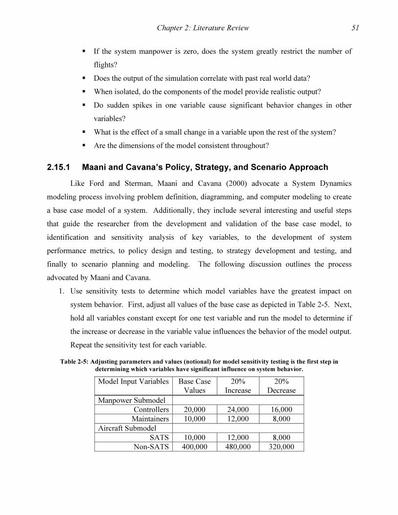
Chapter 2: Literature Review 51
� If the system manpower is zero, does the system greatly restrict the number of
flights?
� Does the output of the simulation correlate with past real world data?
� When isolated, do the components of the model provide realistic output?
� Do sudden spikes in one variable cause significant behavior changes in other
variables?
� What is the effect of a small change in a variable upon the rest of the system?
� Are the dimensions of the model consistent throughout?
2.15.1 Maani and Cavana’s Policy, Strategy, and Scenario Approach
Like Ford and Sterman, Maani and Cavana (2000) advocate a System Dynamics
modeling process involving problem definition, diagramming, and computer modeling to create
a base case model of a system. Additionally, they include several interesting and useful steps
that guide the researcher from the development and validation of the base case model, to
identification and sensitivity analysis of key variables, to the development of system
performance metrics, to policy design and testing, to strategy development and testing, and
finally to scenario planning and modeling. The following discussion outlines the process
advocated by Maani and Cavana.
1. Use sensitivity tests to determine which model variables have the greatest impact on
system behavior. First, adjust all values of the base case as depicted in Table 2-5. Next,
hold all variables constant except for one test variable and run the model to determine if
the increase or decrease in the variable value influences the behavior of the model output.
Repeat the sensitivity test for each variable.
Table 2-5: Adjusting parameters and values (notional) for model sensitivity testing is the first step in
determining which variables have significant influence on system behavior.
Model Input Variables Base Case Values
20% Increase
20% Decrease
Manpower Submodel
Controllers 20,000 24,000 16,000
Maintainers 10,000 12,000 8,000
Aircraft Submodel
SATS 10,000 12,000 8,000
Non-SATS 400,000 480,000 320,000
Chapter 2: Literature Review 52
2. Create system performance metrics based on the original purpose of the model. In the
case of the ATC resource management model, the original purpose was to determine the
behavior of the ATC system under various architectures and the system’s ability to
support SATS flights. Therefore, the following performance metrics may provide a basis
for evaluating the behavior of the modeled system:
a. Aircraft
i. Number of SATS flights
ii. Number of non-SATS flights
b. Manpower
i. Number of controllers
ii. Number of maintenance technicians
c. Equipment
i. Number of radar-based equipment
ii. Number of approved GPS-based equipment
iii. Number of aircraft with GPS capability
d. Facilities
i. Number of SATS airports
ii. Numbers of control towers by type
3. Researchers often use metrics similar to those above to compare the performance of the
system to a benchmark, such as a market. For a monopolistic organization like the air
traffic control system, the benchmark would be a base case of performance at a point in
the system’s history. Therefore, researchers should use the metrics to evaluate the
relative performance of the various model sectors of the system by comparing how new
structure or parameter values shape system behavior relative to the original structure and
parameter values of the base case. Performance metrics frequently include measures
involving ratios of the new case compared to the base case or quantities of components of
the new system.
4. Summarize the results of steps 1 and 2 above by creating a matrix that compares the
performance of each model variable against the base case to highlight the sensitivity of
the model to the particular variable. The comparisons, as depicted in Table 2-6 indicate
the percent change in the system performance metrics in the top row compared to the

Chapter 2: Literature Review 53
model variables in the first column. For example, Table 2-6 shows that within a
submodel of controllers, the number of trainees may have a significant impact on the
behavior of the system, but the number of experienced controllers who switch from the
tower to administrative positions may be irrelevant. Thus, managers would want to focus
on their ability to influence the number of trainees over time. The number of trainees
would be a key variable, but the number of experienced controllers changing from the
control tower to administrative jobs would not.
Table 2-6: The results of the sensitivity tests (notional) provide an indicator of which variables have
significant influence on system behavior and warrant management attention
Model Input Variables Controller Washout # SATS Aircraft SATS Airports
Base Case 5% 5,000 500
20% increase in parameter input values
(%) (% change) (#) (% change) (#) (% change)
Manpower Submodel
Controllers 6% (20%) 5,000 (0%) 500 (0%)
Maintainers 5% (0%) 5,200 (4%) 550 (10%)
Aircraft Submodel
SATS 5% (0%) 23,000 (15%) 1,100 (10%)
Non-SATS 5% (0%) 30,000 (50%) 1,200 (20%)
5. Use the matrix developed in step 4 to identify the endogenous parameters management
should influence and the exogenous parameters management should monitor.
6. Conduct policy experiments. Maani and Cavana refer to policy as “single or localized
changes to the policy parameters in the model or structural changes to the policy
relationships” (p. 236). Accordingly, policy design involves changing parameter values
or the causal structure of the model. If the resultant system behavior is acceptable, then
they describe the policy as “robust.” Because a model with many variables has many
possible policies, Maani and Cavana recommend first, reviewing the purpose for creating
the model to guide the policy analysis process and second, addressing only the policies
that management can influence. Each change in a parameter value or structural
relationship in the model is a policy experiment that creates output for comparison with
the output from the base case model. The collection of robust policies will serve as

Chapter 2: Literature Review 54
possible input for strategy development. The process of conducting policy experiments is
much like conducting additional sensitivity analysis on the most influential variables.
7. Conduct strategy experiments. Maani and Cavana (2000) refer to strategies as “multiple
changes to policy parameters and structures to achieve the strategic objectives set by
management” (p. 236). In the strategy base case, the model incorporates the new or
redesigned system structure, however, the model parameters remain the same as in the
original base case model. Other strategy models also include the new model structure as
well as changes to the parameters that reflect particular strategies, such as shortening
delays or expanding capabilities. Table 2-7 is an example of possible parameters the
managers of the air traffic system may adjust under various strategies. Graphic output
and tabular comparisons of strategy versus system performance metrics helps decision-
makers determine which strategy to employ.
Table 2-7: Notional strategy alternatives using parameters that managers control, such as the number of
trainees in the system, the allocation of funds, and the threshold for goals.
Endogenous Policy Parameters
Strategy 1: Base Case
Strategy 2: Radar Only Control
Strategy 3: GPS only Control
Controller Trainees 5% 2% 12%
Funding for GPS 20% 12% 55%
Max Delay Goal 4% 5% 2%
8. Conduct scenario analysis. Ultimately, Maani and Cavana (2000) advocate the use of
scenario analysis to investigate how “what-if” changes in exogenous variables may affect
the system behavior. Table 2-8 is an example of external values that interact with the air
traffic control system. Scenarios are likely sets of conditions that the system may
encounter in the future. Scenarios capture the decisions and strategies that move a
system toward the future conditions depicted in the scenario. Scenarios are useful to
experiment with policy and strategy alternatives, to create policies and strategies to avoid
undesirable future conditions, and to provide common frameworks for organization-wide
planning. If there are a relatively small number of adjustable external parameters, the
theme of the analysis may be to contrast optimistic scenarios against pessimistic
scenarios. Otherwise, if there are many variables, it may be better to focus on either

Chapter 2: Literature Review 55
optimistic or pessimistic scenarios. As a benchmark against the optimistic or pessimistic
scenarios, researchers should also create a “surprise free” scenario that includes a
description of the future based on assumptions acceptable to all system stakeholders
(Maani & Cavana, 2000).
Table 2-8: Notional scenario input values for external variables that interact with the air traffic control
system.
Exogenous Parameter
Base Case Scenario
Worst Case Scenario
Best Case Scenario
SATS % of IFR Flights
5% 2% 8%
Pool of Controller Candidates
50,000 15,000 300,000
% GPS equipped aircraft
25% 12% 60%
Scenario analysis adds three more steps to the System Dynamics modeling process. First,
researchers should list and categorize the uncertain aspects of the future that may impact upon
the system, such as available population, market prices, demand for services, and working
capital. Candidates for the list will emanate from the exogenous variables in the System
Dynamics model. To focus the list, researchers should chose variables linked to those aspects of
the system that are most likely to occur or those that may have the largest potential impact.
Second, researchers should investigate two to four scenarios consisting of a base case “surprise
free” scenario described above, and at least two extreme cases. The extreme cases may be a
combination of the worst of the worst, the best of the worst, the worst of the best, and the best of
the best. The worst and best policy and strategy experiments provide the input for the worst and
best scenarios. The mental, written, and numerical databases contain information researchers
may use to ensure the parameter values are within reason. Validity tests described above in
section 2.15 are tools to aid researchers in shaping the scenarios. Third, researchers should
compile the results of the scenario analysis in a manner similar to that depicted in Table 2-9 to
summarize and compare the outcomes of the scenarios. Interpretation of the results should
incorporate the original strategic objectives of the managers of the system.

Chapter 2: Literature Review 56
Table 2-9: Results of the notional scenarios contain information comparing the optimistic, pessimistic, or no
surprises scenarios with ATC strategies managers may pursue.
ATC Strategy Base Case Scenario
Worst Case Scenario
Best Case Scenario
Relative Trainee to Controller Ratio
1. Base Case X X+ X-
2. Radar Only Y Y+ Y-
3. 50% GPS Z Z++ Z+
Relative GPS Funding
1. Base Case A A- A+
2. Radar Only B B-- B-
3. 50% GPS C C C++
Relative on-time performance
1. Base Case D D- D
2. Radar Only E E- E
3. 50% GPS F F F+
2.16 System Archetypes
The process of developing a System Dynamics model and using it for experiments and
analysis helps researchers to gain greater understanding of the structure and behavior of systems.
Senge (1990) describes “system archetypes” as common structures that create consistent patterns
of behavior in a wide range of systems in fields as diverse as biology, psychology, politics,
economics, and management. He claims that archetypes are useful to identify where to influence
systems in order to change behavior. Senge (1990) and Senge et al (1994) illustrate a handful of
system archetypes by using simple combinations of balancing loops, reinforcing loops, and
delays to show how simple structure creates universal behavior under certain circumstances.
Sterman (Senge et al, 1994) cautions against relying solely on the archetypes to understand
systems and predict behavior. He sees a danger in fitting archetypes to situations based on
apparent preexisting conditions and then using the archetype as the only tool for diagnosis and
intervention. Forrester (1994) implies that an archetype-only approach is a “superficial” form of
systems thinking that does not lead to true understanding of the dynamic behavior of systems.
Sterman advocates the use of formal models created through a rigorous modeling process for two
reasons. First, people who rely solely on archetypes approach problems as if there is a “multiple-
choice” solution, and second, they would have to intuitively solve high order differential
equations to predict system behavior. Rather, Sterman recommends using causal loop diagrams
and stock and flow diagrams to capture all of the important causality, feedback, and delays in

Chapter 2: Literature Review 57
systems that archetypes may fail to include. Additionally, he describes maps of the system
created by diagrams or archetypes as hypotheses that require testing by means of computer
simulation. Thus, relying exclusively on archetypes can create the conditions that cause people
to “jump to conclusions” (Senge et al, 1994, p. 183). Accordingly, the usefulness of archetypes
appears twofold: first, to initially illustrate the possible causes of system behavior during the
early model application process, and second, to communicate research findings at the end of the
System Dynamics modeling process.
The following section describes some of the archetypes in terms of their structure and the
behavior they produce. Some archetypes involve growth through reinforcing loops; others
address problem solving by orienting on balancing loops. The illustrative examples are issues
relevant to managers of the ATC system and are concerns that those planning to use the NAS
may consider.
2.16.1 The Limits to Growth Archetype
Limits to growth occur when an activity that produces a desired effect becomes offset by
a constrained counterbalancing activity (Senge, 1990; Senge et al, 1994). Figure 2-12 below is
an example of the limits to growth archetype. The reinforcing loop on the left links passenger
flow to revenue then back to passenger flow. Airlines initiatives, such as advertising or
expansion, could attract more passengers and increase revenue. However, limited runway
capacity eventually may cause delays that result in passenger dissatisfaction resulting in fewer
airline passengers because people opt for another mode of transportation or substitute a
teleconference for a business trip.
PassengersAirline RevenueOn-time
Satisfaction
Runway
Capacity
R B
Figure 2-12. The limits to growth archetype consist of growth through the reinforcing loop on the left
counteracted by the balancing loop on the right, which has a vertical mark indicating a delay.

Chapter 2: Literature Review 58
The structure of the system characterized by the limits to growth archetype causes key
variables to initially improve as desired and then plateau or deteriorate. Figure 2-13 is an
example of the typical pattern of behavior.
Figure 2-13. The typical pattern of behavior caused by the limits to growth system archetype includes a
period of favorable behavior followed by a plateau or deterioration.
Senge (1990) and Senge et al (1994) recommend several strategies to overcome the limits
to growth. First, address the limiting condition in the system, such as the runway capacity above,
to change the system behavior. Second, refrain from the natural tendency to push harder on the
reinforcing loop activities, such as increasing advertising or expanding airline operations,
because they will only cause the balancing loop to strengthen as well. Third, after removing a
limit to growth, attempt to determine what other limits to growth may also reside in the system
and address them. Finally, look for other reinforcing loops that may provide new opportunities
for growth.
2.16.2 The Tragedy of the Commons Archetype
The tragedy of the commons occurs when many individuals initially benefit from an
easily accessible common resource until it becomes overused, less beneficial, and eventually
depleted (Senge, 1990; Senge et al, 1994). Figure 2-14 is an example of the tragedy of the
commons archetype. The upper and lower reinforcing loops represent growing airlines that are
adding more flights to their schedule. Eventually, they may use up the limited airspace available
in the NAS.
Revenue
Time
desired
plateau
deterioration

Chapter 2: Literature Review 59
Airline 2 Flights
Airspace 2
Required
Airspace Available
per Airline
National Airspace
System Capacity
R
Total Airspace
Required by Airlines
Airspace 1
Required
Airline 1 FlightsR
B
B
Figure 2-14. The tragedy of the commons archetype consists of growing individual airlines, depicted in the
upper and lower reinforcing loops, constrained by the common resource of airspace available in the national
system.
The structure of the system characterized by the tragedy of the commons archetype
includes a period of favorable behavior followed by a decline as more individuals compete for
the same limited resource. Figure 2-15 is an example of the typical pattern of behavior.
Figure 2-15. The typical pattern of behavior caused by the tragedy of the commons system archetype
includes a period of favorable behavior followed by a decline as more individual airlines compete for the
same limited resource.
Total Airspace
Usage
Time
Each Airline’s
Share of Airspace
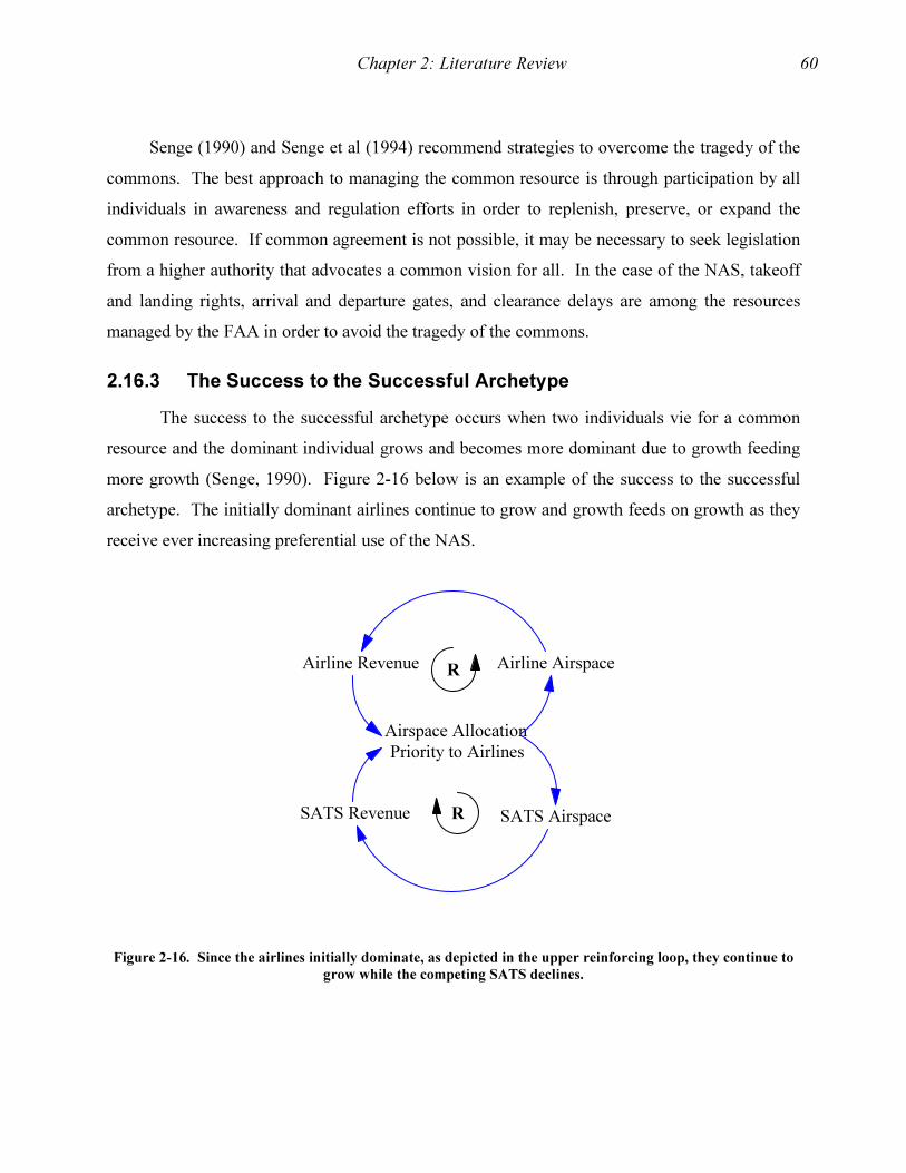
Chapter 2: Literature Review 60
Senge (1990) and Senge et al (1994) recommend strategies to overcome the tragedy of the
commons. The best approach to managing the common resource is through participation by all
individuals in awareness and regulation efforts in order to replenish, preserve, or expand the
common resource. If common agreement is not possible, it may be necessary to seek legislation
from a higher authority that advocates a common vision for all. In the case of the NAS, takeoff
and landing rights, arrival and departure gates, and clearance delays are among the resources
managed by the FAA in order to avoid the tragedy of the commons.
2.16.3 The Success to the Successful Archetype
The success to the successful archetype occurs when two individuals vie for a common
resource and the dominant individual grows and becomes more dominant due to growth feeding
more growth (Senge, 1990). Figure 2-16 below is an example of the success to the successful
archetype. The initially dominant airlines continue to grow and growth feeds on growth as they
receive ever increasing preferential use of the NAS.
SATS AirspaceSATS Revenue R
Airspace Allocation
Priority to Airlines
Airline Revenue Airline AirspaceR
Figure 2-16. Since the airlines initially dominate, as depicted in the upper reinforcing loop, they continue to
grow while the competing SATS declines.

Chapter 2: Literature Review 61
The behavior of the system characterized by the success to the successful archetype
shows increased growth by the initially dominant individual and decline by the other competing
individual. Figure 2-17 is an example of the typical pattern of behavior.
Figure 2-17. The typical pattern of behavior caused by the success to the successful system archetype involves
a divergence of performance as the airlines’ initial dominance feeds growth.
Senge (1990) recommends strategies to overcome the success to the successful challenge.
He recommends seeking a higher goal that the competing individuals may both pursue with
mutual advantage. An agreement to complement each other with connecting flights may be one
such solution. Otherwise, an opposite strategy is to reduce the competition for the common
resource by reorienting one on another resource, such as providing separate airspace or airfields
for SATS and the airlines.
Archetypes may be useful to guide the development of the model as well as interpret the
model output. Archetypes, used in concert with system diagrams, help explain system behavior
during model development and application. Graphically oriented System Dynamics software
packages include symbols for illustrating archetypes as well as causal mapping capabilities to
trace the flows of influence through models. Further exploration of System Dynamics software
will help to determine which software may best suit the overall modeling and system analysis
effort.
2.17 System Dynamics Software
Ford (1999) discusses four commercial software packages designed specifically for System
Dynamics modeling. The software packages Stella, Vensim, and Powersim all use icon-based
Time
Airline Revenue
SATS “Airline”
Revenue
Chapter 2: Literature Review 62
graphical interfaces to make the model building process visual and intuitively simpler than the
equation-based approach of DYNAMO. The DYNAMO software evolved form mainframe
computers as the original System Dynamics modeling language in the 1960s. The Ventanna
consulting firm developed Vensim to support their consulting efforts and to use it as a tool to
communicate with clients. Stella and Vensim are compatible on both MacIntosh and personal
computers, however, Powersim will not run on a MacIntosh computer. Powersim interfaces well
with other windows applications through dynamic data exchange, object linking and embedding,
and application programmer’s interfaces. Ford prefers Stella and he uses it to demonstrate
modeling throughout his text. He appears to favor the ease of creating modeling diagrams and
interfaces with Stella, although he praises the unique capabilities of Vensim and the
interconnectivity of Powersim with other windows programs.
Coyle’s (1996) remarks about System Dynamics software, although dated in terms of
software capabilities, provide worthwhile insight regarding not only the features one should seek,
but also pitfalls to avoid in using the software. He claims that it is more important to use the
software properly than to worry about which package one chooses to use. Accordingly, he
focuses on the factors that relate to sound System Dynamics modeling: proper equations,
appropriate units, thorough documentation, debugging capabilities, and the ability to experiment.
In his view, the software packages break down into two camps, the first being text-based
software such as Dynamo, COSMIC, and DYSMAP2. The second camp consists of the
graphics-based software: Stella, Powersim, and Vensim. Although he highlights the advantages
and clarity of creating graphic displays of models, he strongly cautions modelers not to be too
quick to create a model without thoroughly ensuring that the equations and units accurately
represent the system being modeled. Thus, his concerns lie primarily in the area of model
validation because he fears the graphical approach makes it too easy to build bad models. He
makes two recommendations, first, modelers should consider using more than one software
package, and second, modelers should patiently learn how to use the software before using it in a
“serious model.”
Although Sterman (2000) does not discuss System Dynamics software packages, a
compact disc containing ithink, Powersim, and Vensim accompanies his text. As one of the
leading System Dynamics theorists, his tacit endorsement of the three packages places them high
in the hierarchy of software and adds considerable credibility to the use of the graphically
Chapter 2: Literature Review 63
oriented approach. Sterman’s thorough treatment of model validity and proper model
development addresses Coyle’s admonitions regarding the possibility of building visually
attractive, but flawed models. Thus, the graphic approach is here to stay and it is the model
builder’s responsibility to attend to the nuances of equation writing and unit integrity to create a
good product.
The above discussion combined with prior experience and software availability makes
Vensim the software of choice for the modeling of future ATC system behavior. The Vensim
software offers the ability to create causal loop diagrams, stock and flow diagrams, and
simulation experiments. The software has built in checks to ensure consistency of units, proper
equation structure, and user definable “reality checks” to address model validity. Nevertheless,
despite the functionality of the software, the software is a tool and the essence of the System
Dynamics modeling effort consists of how well the modeler can apply the process of
representing a real world system as a model.
2.18 Summary
The literature review provides the context for the impact of SATS on the air traffic control
system. The FAA and NASA have ambitious plans for the future of aviation. NASA is
advocating revolutionary technological advances, while the FAA seeks a more evolutionary
approach that emphasizes the need for safety in current operations. The history of air traffic
control is one of irregular resource management, reactionary approaches to crises, and initially
marginal success with new technology.
The literature review also addresses the activities involved in air traffic control, modeling
efforts related to this study, and problems experienced by the European ATC system. The
background, issues, and related research leads to the conclusion that the systems approach is a
valid and feasible manner of addressing the issue of how managers can influence future ATC
systems, support the needs of SATS and non-SATS aircraft, and generate revenue to fund the
ATC system.
The systems approach leads to the application of System Dynamics as a model
development process to investigate the future behavior of the ATC system under various
scenarios. As a maturing field, the body of knowledge that guides researchers in the proper
application of the System Dynamics approach is scattered among the works of theorists and

Chapter 2: Literature Review 64
practitioners. An overview of their work sets the stage for sound modeling practices that will
lead to insight for managers to adapt policies that will create desirable results. The next chapter
will provide the blueprint to create a System Dynamics model.

65
3.1 Research Design Overview
The research design is a plan consisting of the step-by-step procedures to apply a
methodology to interpret the meaning of data (Leedy, 2001). The methodology will combine the
System Dynamics modeling process along with computer simulation experiments. The mental,
written, and numerical databases will provide the information needed to build and validate the
model (Forrester, 1991). Users of the model will be able to create data representing the future
behavior of the ATC system under a predominantly radar or GPS-based NAS to determine the
number of SATS aircraft the system may support. The output of the model will be useful to
evaluate various policy and strategy alternatives. The model will also be useful as a management
tool to understand the conditions associated with possible future scenarios. Figure 3-1 provides
an overview of the research design.
Figure 3-1. The research design is a plan to develop the model, test the model, use the model for policy and
strategy experimentation, and conduct scenario analysis.
Chapter 3: Research Design
Structure & Parameters
Method
System Dynamics
Model Development Process
System Dynamics Model
Computer Simulation
Experiments
Mental
Written
Numeric
Data
Model
Experiment
Validity&
Sensitivity
Policy, Strategy, &
Scenario Analysis

Chapter 3: Research Methodology 66
3.2 The System Dynamics Modeling Process
The System Dynamics modeling process described in Chapter 2 and outlined below
includes the steps needed to create and validate a computer simulation model of air traffic
control in a future radar or GPS-based NAS with or without a SATS presence. The mental,
written, and numeric databases associated with air traffic control will serve as a source of
information to develop and validate a System Dynamics model. The mental models of
stakeholders and subject matter experts will help to reveal how the air traffic control system
operates and how they understand decision-making to occur within the system. Accordingly,
interviews using a procedure similar to that advocated by Ford & Sterman (1998) will supply a
portion of the data to construct the model. The written database will also serve as a source of
information to capture important nuances in the design of the system. The numeric database will
contain evidence to support parameter development and serve as a benchmark for evaluating
model output. Fundamentally, the role of the researcher will be to manage the System Dynamics
modeling process in order to develop insights and encourage innovation in the use of policies
related to manning the nation’s air traffic control system (Schrage, 2000).
The following discussion outlines the step-by-step process of developing a good model.
It is important to recognize that the process is iterative. The researcher’s goal is to use the
process to ultimately generate numeric and graphic output showing cause and effect relationships
among key variables in the NAS that influence the behavior of the ATC system. The procedures
stem from the discussion in Chapter 2 above and reflect the concepts espoused by Forrester,
Sterman, Ford, Campbell, Homer, and others.
3.2.1 Step 1: Problem Definition
Like all scientific research endeavors, the System Dynamics modeling process begins with a
definition of the dynamic problem. To be dynamic, the problem must change over time. If the
problem is not dynamic, another approach such as linear programming may be appropriate.
1. Identify the individual or group with the dynamic problem.
a. Determine how the client likes to communicate.
b. Determine how the client is addressing the problem.
c. Identify other computer models the client may be using.
Chapter 3: Research Methodology 67
d. Identify who within the client’s organization has the power to accept and
implement findings from the modeling effort.
2. Define the dynamic problem and why it is a problem.
a. Identify key variables in the system.
b. Determine the time horizon over which the problem influences the system.
3. Develop a dynamic hypothesis that describes the problem as a result of the relationship
among the variables and internal structure of the system.
a. Develop reference modes to graphically depict the undesirable behavior over
time.
b. Draw an additional curve on the reference mode graphs that show improved
behavior.
4. Develop performance measurement metrics that will help to determine the effectiveness
of the System Dynamics approach to the problem.
3.2.2 Step 2: System Description
Researchers use mapping tools to determine the structure of the system and to identify
endogenous, exogenous and excluded variables. Modelers may revise the system description as
they gain more insight from subsequent steps in the modeling process.
1. Interview stakeholders and subject matter experts.
a. Determine where and how information flows through the system.
b. Determine where decision-making occurs.
c. Describe the roles of people in the system.
2. Conduct a literature review.
a. Seek information from the mainstream media as well as academic journals.
b. Incorporate information from relevant case studies.
3. Assemble numerical data.
a. Obtain data that will be useful to estimate parameters, describe stocks, or provide
past averages or ratios of system variables.
b. Include data derived from scientific constants, results of experiments, or statistical
analysis of databases.

Chapter 3: Research Methodology 68
4. Create diagrams of the system using commercially available System Dynamics modeling
software.
a. Develop stock and flow diagrams of the whole system and its subsystems to
describe the key variables, relationships, and structure in the system.
i. Identify the stocks.
ii. Determine the flows.
iii. Add the auxiliary variables.
b. Develop causal loop diagrams of the whole system and its subsystems to highlight
the feedback loops in the system.
c. Use a model boundary chart to categorize variables as endogenous, exogenous, or
excluded.
d. Create policy structure diagrams to determine how information prompts decision-
making within the system.
5. Present the results of the above diagramming efforts to stakeholders and subject matter
experts.
a. Receive feedback on the conceptual descriptions of the system.
b. Make adjustments as necessary.
3.2.3 Step 3: Build a Simulation Model
To build a System Dynamics model, the modeler seeks the appropriate level of dynamic
complexity while trying to avoid getting too wrapped up with detail complexity. Model building
is both an art and a science. The modeler should start with a simple model then add more
complexity until the model replicates the system.
1. Use the stock and flow diagrams developed above and the System Dynamics software as
the basis for the simulation model.
a. Determine mathematical relationships among the variables in the model by
interpreting the results of the inquiries into the mental, written, and numeric
databases. Convert verbal, written, and numeric descriptions of the system to
mathematical relationships.
b. Use statistical tests to determine model parameters when numeric data is
available.
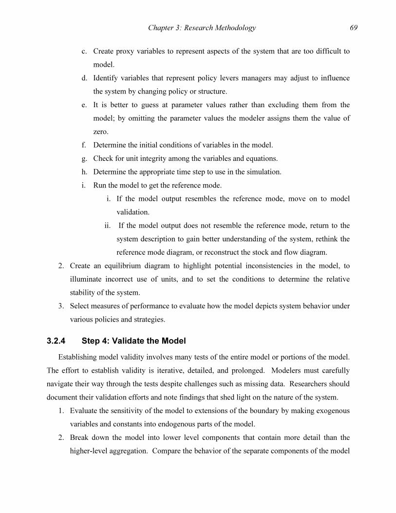
Chapter 3: Research Methodology 69
c. Create proxy variables to represent aspects of the system that are too difficult to
model.
d. Identify variables that represent policy levers managers may adjust to influence
the system by changing policy or structure.
e. It is better to guess at parameter values rather than excluding them from the
model; by omitting the parameter values the modeler assigns them the value of
zero.
f. Determine the initial conditions of variables in the model.
g. Check for unit integrity among the variables and equations.
h. Determine the appropriate time step to use in the simulation.
i. Run the model to get the reference mode.
i. If the model output resembles the reference mode, move on to model
validation.
ii. If the model output does not resemble the reference mode, return to the
system description to gain better understanding of the system, rethink the
reference mode diagram, or reconstruct the stock and flow diagram.
2. Create an equilibrium diagram to highlight potential inconsistencies in the model, to
illuminate incorrect use of units, and to set the conditions to determine the relative
stability of the system.
3. Select measures of performance to evaluate how the model depicts system behavior under
various policies and strategies.
3.2.4 Step 4: Validate the Model
Establishing model validity involves many tests of the entire model or portions of the model.
The effort to establish validity is iterative, detailed, and prolonged. Modelers must carefully
navigate their way through the tests despite challenges such as missing data. Researchers should
document their validation efforts and note findings that shed light on the nature of the system.
1. Evaluate the sensitivity of the model to extensions of the boundary by making exogenous
variables and constants into endogenous parts of the model.
2. Break down the model into lower level components that contain more detail than the
higher-level aggregation. Compare the behavior of the separate components of the model
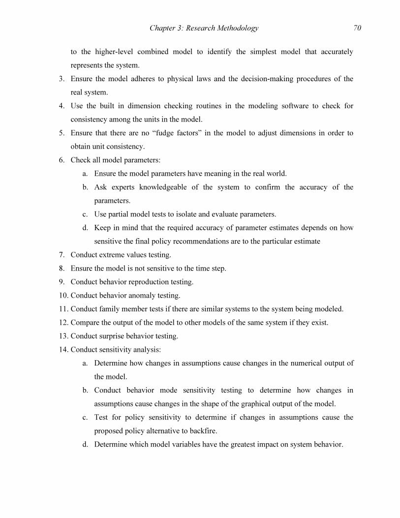
Chapter 3: Research Methodology 70
to the higher-level combined model to identify the simplest model that accurately
represents the system.
3. Ensure the model adheres to physical laws and the decision-making procedures of the
real system.
4. Use the built in dimension checking routines in the modeling software to check for
consistency among the units in the model.
5. Ensure that there are no “fudge factors” in the model to adjust dimensions in order to
obtain unit consistency.
6. Check all model parameters:
a. Ensure the model parameters have meaning in the real world.
b. Ask experts knowledgeable of the system to confirm the accuracy of the
parameters.
c. Use partial model tests to isolate and evaluate parameters.
d. Keep in mind that the required accuracy of parameter estimates depends on how
sensitive the final policy recommendations are to the particular estimate
7. Conduct extreme values testing.
8. Ensure the model is not sensitive to the time step.
9. Conduct behavior reproduction testing.
10. Conduct behavior anomaly testing.
11. Conduct family member tests if there are similar systems to the system being modeled.
12. Compare the output of the model to other models of the same system if they exist.
13. Conduct surprise behavior testing.
14. Conduct sensitivity analysis:
a. Determine how changes in assumptions cause changes in the numerical output of
the model.
b. Conduct behavior mode sensitivity testing to determine how changes in
assumptions cause changes in the shape of the graphical output of the model.
c. Test for policy sensitivity to determine if changes in assumptions cause the
proposed policy alternative to backfire.
d. Determine which model variables have the greatest impact on system behavior.

Chapter 3: Research Methodology 71
15. Ask an independent party to run the model on a different computer to verify that the
model operates as intended.
a. Ask them to check the programming.
b. Ask them to check the documentation.
16. Ask experts to review the model to verify that the model structure, parameters and
behavior replicate the system being modeled.
a. Expect some experts to transition through a period of realigning their mental
models of the system with the behavior depicted by the System Dynamics model
of the system.
b. Reassure those associated with the model that the challenging transition of
realigning mental models is a normal part of the process.
17. Be aware of stakeholders who desire to use the model to validate their preconceived
notions of how they believe the system behaves.
18. Determine if the application of the model resulted in improved system performance
according to the process effectiveness metrics developed above in the problem definition
outlined in section 3.2.1.
3.3 Computer Simulation Experimentation
In this phase of the process the researcher moves beyond just creating and handling data.
The researcher uses insights gained from the modeling effort to begin thinking about new ways
of addressing the problem.
3.3.1 Step 5: Establish a Base Case
The base case is the result of the iterative model development efforts and it is a reproduction
of the reference mode.
1. Define the base case in terms of specific values for all of the key variables in the model.
2. Identify whether variables are endogenous or exogenous. Indicate the degree of
influence management has on each variable.
3. Define the benchmark or base case of performance against which to compare other runs
of the model after making structural or parameter value adjustments to it.
4. Create system performance metrics based on the original purpose of the model.

Chapter 3: Research Methodology 72
3.3.2 Step 6: Conduct Policy Experiments
Policy changes occur when modelers change individual endogenous parameter values or the
structure of a model to create new behavior.
1. Review the purpose for creating the model to guide the policy analysis process.
2. Address only the policies that management can influence.
3. Change parameter values and compare the output with the base case of the model.
4. Change model structure and compare the output with the base case of the model.
5. Conduct visual inspection of output and statistical tests to determine if there is a
significant difference in the behavior of the system under the various policies. Record
the results of the experiments and identify the policies that are robust.
3.3.3 Step 7: Conduct Strategy Experiments
Strategy changes occur when modelers change combinations of endogenous parameter values
or make multiple changes to the structure of a model to create new behavior.
1. Update the model base case to include the structural changes made as a result of policy
experiments.
2. Keep model parameters the same as in the original base case.
3. Make combinations of parameter and structural adjustments to the new base case and
compare them to the base case.
4. Evaluate the strategy against the system performance metrics.
5. Conduct visual inspection of output and statistical tests to determine if there is a
significant difference in the behavior of the system under the various strategies. Record
the results of the experiments and identify the strategies that are most beneficial.
3.3.4 Step 8: Conduct Scenario Analysis
Use scenario analysis to investigate how “what-if” changes in exogenous variables may
affect the system behavior.
1. Identify the exogenous variables in the system.
2. Determine if the theme of the scenario analysis will be optimistic versus pessimistic or
consist of varying degrees of either optimism or pessimism.
3. Create a surprise free scenario.
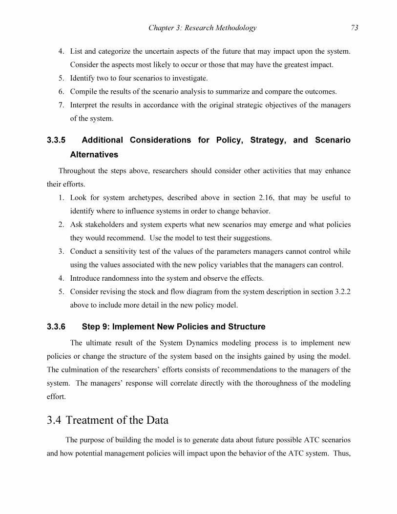
Chapter 3: Research Methodology 73
4. List and categorize the uncertain aspects of the future that may impact upon the system.
Consider the aspects most likely to occur or those that may have the greatest impact.
5. Identify two to four scenarios to investigate.
6. Compile the results of the scenario analysis to summarize and compare the outcomes.
7. Interpret the results in accordance with the original strategic objectives of the managers
of the system.
3.3.5 Additional Considerations for Policy, Strategy, and Scenario
Alternatives
Throughout the steps above, researchers should consider other activities that may enhance
their efforts.
1. Look for system archetypes, described above in section 2.16, that may be useful to
identify where to influence systems in order to change behavior.
2. Ask stakeholders and system experts what new scenarios may emerge and what policies
they would recommend. Use the model to test their suggestions.
3. Conduct a sensitivity test of the values of the parameters managers cannot control while
using the values associated with the new policy variables that the managers can control.
4. Introduce randomness into the system and observe the effects.
5. Consider revising the stock and flow diagram from the system description in section 3.2.2
above to include more detail in the new policy model.
3.3.6 Step 9: Implement New Policies and Structure
The ultimate result of the System Dynamics modeling process is to implement new
policies or change the structure of the system based on the insights gained by using the model.
The culmination of the researchers’ efforts consists of recommendations to the managers of the
system. The managers’ response will correlate directly with the thoroughness of the modeling
effort.
3.4 Treatment of the Data
The purpose of building the model is to generate data about future possible ATC scenarios
and how potential management policies will impact upon the behavior of the ATC system. Thus,

Chapter 3: Research Methodology 74
there is a requirement to use numerical data and relationships among the components of the
system to build and validate the model. Additionally, the model will be a source of data. The
literature review in chapter 2 addressed both the data for building and the data for policy
development. The following discussion contains a summary of the data requirements, data
management procedures, and data analysis procedures in order to determine how much support
future radar or GPS-based ATC systems will provide to SATS aircraft.
3.4.1 Data Requirements
The data requirements emanate from the main components of the air traffic control system
replicated in the System Dynamics model. As model development progresses, data requirements
will evolve. Data requirements will be both relational, such as how many controllers work in a
control tower, and longitudinal, such as the annual number of controllers in the FAA over time.
Anticipated data requirements to support the model development are as follows:
1. Personnel submodel
1) Numbers and types of air traffic controllers and maintenance technicians over
time
2) Controllers and maintainers required for each type of facility or piece of
equipment
3) Controller training data
2. Budget Submodel
1) FAA budgets
2) Airport and Airways Trust Fund
3) Revenue per type of aircraft
4) Controller costs over time
5) ATC equipment costs of time
6) Airport costs over time
3. Aircraft submodel
1) Numbers and types of aircraft over time
2) SATS aircraft fielding projections
4. Equipment submodel
1) Numbers and types of radar-based equipment

Chapter 3: Research Methodology 75
2) Numbers and types of GPS equipment
3) ATC equipment capabilities and fielding schedule
4) Aircraft navigation equipment capabilities
5. Facilities submodel
1) Numbers and types of facilities
2) Controllers required per type of facility
3) Equipment required per type of facility
Section 3.3 above describes the development and treatment of the data for the policy
experiments, strategy experiments, and scenario analysis.
3.4.2 Data Management
The data to build and validate the model comes from the mental, written, and numerical
databases. Ultimately, the compilation of the data resides in the mathematical relationships
embedded in the software of the System Dynamics model. For explanatory purposes, the data
used in the model is in the discussion in Chapter 4 or in a summary appendix to the research
documentation in either spreadsheet format or as mathematical expressions showing
relationships among components of the model. Otherwise, the capabilities of the System
Dynamics software allow modelers to use graphic user interfaces to easily insert and access the
data in the model.
3.4.3 Data Analysis
Data analysis falls into two primary categories: 1) analysis of data to build the model; and
2) analysis of data generated by the model. Since the type and format of the data is similar in
both categories, the analysis procedures will also be similar. The data analysis procedures will
involve analysis of tabular data, visual graphical analysis, statistical techniques such as
regression, and the use of output from other studies and models. Additionally, the System
Dynamics software includes the capability to conduct various forms of output analysis.
3.5 Expected Results
At a minimum, the products of the research effort will include a System Dynamics model of
the components of the air traffic control system that demonstrates how the system may behave

Chapter 3: Research Methodology 76
under various resource management strategies. Additionally, the research will result in a
compilation of the salient mental models, written perspectives, and numerical data that describe
the flow of resources and revenue through the ATC system. Finally, the research will produce
knowledge of the potential ramifications of changes to policies associated with the ATC system
and its ability to support SATS aircraft and generate sufficient revenue for the Airport and
Airways Trust Fund.
The impact of the results will provide new insight for decision-makers at the FAA and
NASA regarding the introduction of the small aircraft transportation system under various ATC
resource management strategies. The insights may serve as a bridge between the aggressive,
revolutionary vision proposed by NASA and the cautious, evolutionary perspective practiced by
the FAA. Although, both government agencies share the goal of improving the use of the NAS,
they choose to pursue the goal in fundamentally different ways. Subsequently, neither agency is
taking a hard look at the relationships among SATS and the behavior of future ATC systems.
The NASA SATS advocates assume that technology will solve any ATC problems and the FAA
administrators see no ATC requirement because SATS is merely conceptual. The research
proposed in this document will objectively highlight the emerging issues and identify potential
problems that may lie ahead. The development of the System Dynamics model in the next
chapter is the first step toward obtaining research results.
77
4.1 System Dynamics Model Development Process
The NASA advocates of SATS proposed the system as an intervention to alleviate the
delays incurred by travelers who use the hub and spoke system. However, from a systems
thinking perspective, one realizes that interventions often have desired effects and undesired side
effects. The undesired side effects usually emanate from “policy resistance, the tendency for
interventions to be defeated by the response of the system to the intervention itself” (Sterman,
2001, p.8). The response of the large and complex air traffic control system to architectural
changes and the influx of SATS aircraft may result in unanticipated side effects due to the
inherent feedback structure of the ATC system and delayed responses caused by changes to the
flow of resources and revenue through the system. Accordingly, the System Dynamics modeling
process offers an approach that can capture the behavior of the ATC system by means of a
computer model that replicates the system structure and the entities that flow through it.
The flowchart in Figure 4-1 depicts nine steps modelers use to define a problem, create a
model, and apply the model to recommend actions that may improve system behavior. The
modeling process involves iteration, particularly among the first three steps, to refine the effort
as feedback from the real world invokes the need to make changes. The art of modeling requires
the modeler to discern the nature of the system through study, discussion, and numerical
analysis. The science of modeling requires the modeler to develop parameters for the model,
validate the model, and apply it to investigate system behavior. An important aspect of the art
and science of the modeling effort is to determine the appropriate level of aggregation and
analysis of the components of the system in order to create a valid and useful replication of the
real world.
4.2 Levels of analysis
The concept of “levels of analysis” is a relevant issue for any modeling effort and is an
important concern in the development of a System Dynamics model. A survey of the simulation
Chapter 4: The ATC Resource Management
Model

Chapter 4: The ATC Manpower & Infrastructure Resource Management Model 78
modeling literature indicated that the inclination of most modelers was to use the broadest scope
and greatest level of detail when creating models (Chwif, Barretto, & Paul, 2000). However,
Law and Kelton (2000) discourage replicating every element of a system in a model prior to
defining the purpose of the study, determining the modeled performance metrics to evaluate, and
fully consulting with managers and subject matter experts associated with the study. Klein,
Dansereau, and Hall (1994) describe how conclusions drawn about a variety of organizational
research issues; in areas such as personnel management, technology, and organizational
performance; resulted in findings that varied according to the level of analysis.
Figure 4-1: Steps of the System Dynamics Modeling Process lead modelers from problems to solutions (Maani
and Cavana, 2000).
The “levels of analysis” framework proposed by Klein, Dansereau, and Hall (1994)
describes the “levels of analysis” concept and highlights why it is important to organizational
research and modeling. They define the “level of theory” as the intended person, team, or
organization that a modeler seeks to replicate and elucidate; the “level of measurement” as the
point at which the data originated; and the “level of statistical analysis” as the point at which the
researcher aggregates data for analysis. The word “point” means the level of aggregation of
people, such as the individual, dyad, team, group, organization, community, or beyond, which
Klein et al. refer to as an “entity.” Thus, an entity is not just an individual person. An entity
may be any collection of people provided it represents a particular level at which a researcher
may apply theory, collect data, or conduct statistical analysis. Dansereau, Alutto, and
Define Problem
Describe System
Build Model
Verify/Validate Model
Policy Experiments
Establish Base Case
Strategy Experiments
Scenario Analysis
Recommend Actions
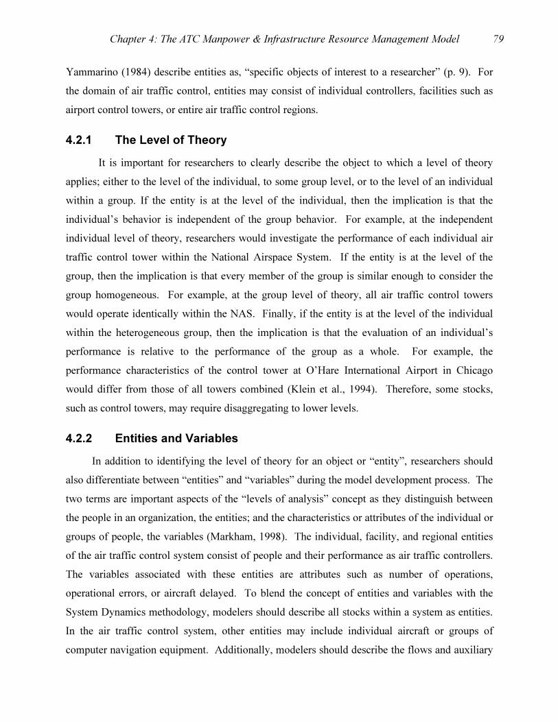
Chapter 4: The ATC Manpower & Infrastructure Resource Management Model 79
Yammarino (1984) describe entities as, “specific objects of interest to a researcher” (p. 9). For
the domain of air traffic control, entities may consist of individual controllers, facilities such as
airport control towers, or entire air traffic control regions.
4.2.1 The Level of Theory
It is important for researchers to clearly describe the object to which a level of theory
applies; either to the level of the individual, to some group level, or to the level of an individual
within a group. If the entity is at the level of the individual, then the implication is that the
individual’s behavior is independent of the group behavior. For example, at the independent
individual level of theory, researchers would investigate the performance of each individual air
traffic control tower within the National Airspace System. If the entity is at the level of the
group, then the implication is that every member of the group is similar enough to consider the
group homogeneous. For example, at the group level of theory, all air traffic control towers
would operate identically within the NAS. Finally, if the entity is at the level of the individual
within the heterogeneous group, then the implication is that the evaluation of an individual’s
performance is relative to the performance of the group as a whole. For example, the
performance characteristics of the control tower at O’Hare International Airport in Chicago
would differ from those of all towers combined (Klein et al., 1994). Therefore, some stocks,
such as control towers, may require disaggregating to lower levels.
4.2.2 Entities and Variables
In addition to identifying the level of theory for an object or “entity”, researchers should
also differentiate between “entities” and “variables” during the model development process. The
two terms are important aspects of the “levels of analysis” concept as they distinguish between
the people in an organization, the entities; and the characteristics or attributes of the individual or
groups of people, the variables (Markham, 1998). The individual, facility, and regional entities
of the air traffic control system consist of people and their performance as air traffic controllers.
The variables associated with these entities are attributes such as number of operations,
operational errors, or aircraft delayed. To blend the concept of entities and variables with the
System Dynamics methodology, modelers should describe all stocks within a system as entities.
In the air traffic control system, other entities may include individual aircraft or groups of
computer navigation equipment. Additionally, modelers should describe the flows and auxiliary

Chapter 4: The ATC Manpower & Infrastructure Resource Management Model 80
variables as the variables that describe the characteristics of the stocks, for example, training
time for new controllers, aircraft navigation equipment capabilities, or time to deploy a new
computer system. The System Dynamics process facilitates the identification of entities and
variables. It is important to discern the difference between entities and variables in order to
apply theory, make measurements, and conduct statistical analysis at the appropriate entity level.
The discussion above identifies several issues to deal with in the model development
effort. First, what level of theory will the model address: individual controller, facility, region,
or the entire system? Second, from what level in the system do the data emanate? Third, at what
level will the modeler aggregate the data to conduct analysis? Fourth, are entities within the
system independent, homogenous, or heterogeneous? And fifth, what are the variables
associated with the entities? Since the System Dynamics model of the air traffic control system
will center on the homogeneity of entities within the system, it is important to determine at what
level the entities are indeed homogeneous. The overview of the system in the next section
provides the bounds within which to identify ATC entities and the levels of analysis best suited
for them.
4.3 Model Overview
The purpose of the model is to determine what air traffic control resource management
strategy will support the future needs of the Small Aircraft Transportation System and create
adequate tax revenue to fund the Federal Aviation Administration. The model should replicate
the behavior of the system to determine how it behaves with or without the presence of SATS
aircraft. Thus, the components of the model must reflect both the current ATC system with non-
SATS aircraft and the likely ATC system of the future with both SATS and non-SATS aircraft.
Additionally, to be useful to those who develop policies for the ATC system, the model should
contain the capability to include exogenous variables, such as the amount of funding for GPS
equipment, in the system that managers can influence to ascertain the response of the system to
manipulations that reflect resource management strategies. The researcher attempted to include
all of these characteristics through a series of iterations and embellishments that resulted in the
system level model depicted in Figure 4-2.
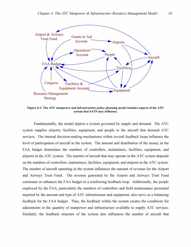
Chapter 4: The ATC Manpower & Infrastructure Resource Management Model 81
Airport & Airways
Trust Fund
Congress
FAA Budget
Airports
Facilities
People
Equipment
Aircraft
Resource Management
Strategy
Grants in Aid
Account
Operations
Account
Facilities &
Equipment Account
Figure 4-2: The ATC manpower and infrastructure policy planning model includes aspects of the ATC
system that SATS may influence.
Fundamentally, the model depicts a system governed by supply and demand. The ATC
system supplies airports, facilities, equipment, and people to the aircraft that demand ATC
services. The internal decision-making mechanisms within several feedback loops influence the
level of participation of aircraft in the system. The amount and distribution of the money in the
FAA budget determines the numbers of controllers, maintainers, facilities, equipment, and
airports in the ATC system. The number of aircraft that may operate in the ATC system depends
on the numbers of controllers, maintainers, facilities, equipment, and airports in the ATC system.
The number of aircraft operating in the system influences the amount of revenue for the Airport
and Airways Trust Fund. The revenue generated by the Airport and Airways Trust Fund
constrains or enhances the FAA budget in a reinforcing feedback loop. Additionally, the people
employed by the FAA, particularly the numbers of controllers and field maintenance personnel
required by the amount and type of ATC infrastructure and equipment, also serve as a balancing
feedback for the FAA budget. Thus, the feedback within the system creates the conditions for
adjustments in the quantity of manpower and infrastructure available to supply ATC services.
Similarly, the feedback structure of the system also influences the number of aircraft that
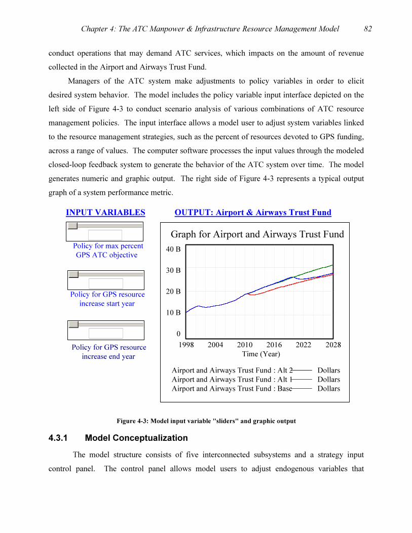
Chapter 4: The ATC Manpower & Infrastructure Resource Management Model 82
conduct operations that may demand ATC services, which impacts on the amount of revenue
collected in the Airport and Airways Trust Fund.
Managers of the ATC system make adjustments to policy variables in order to elicit
desired system behavior. The model includes the policy variable input interface depicted on the
left side of Figure 4-3 to conduct scenario analysis of various combinations of ATC resource
management policies. The input interface allows a model user to adjust system variables linked
to the resource management strategies, such as the percent of resources devoted to GPS funding,
across a range of values. The computer software processes the input values through the modeled
closed-loop feedback system to generate the behavior of the ATC system over time. The model
generates numeric and graphic output. The right side of Figure 4-3 represents a typical output
graph of a system performance metric.
Policy for GPS resource
increase start year
Graph for Airport and Airways Trust Fund
40 B
30 B
20 B
10 B
0
1998 2004 2010 2016 2022 2028
Time (Year)
Airport and Airways Trust Fund : Alt 2 Dollars
Airport and Airways Trust Fund : Alt 1 Dollars
Airport and Airways Trust Fund : Base Dollars
INPUT VARIABLES OUTPUT: Airport & Airways Trust Fund
Policy for max percent
GPS ATC objective
Policy for GPS resource
increase end year
Figure 4-3: Model input variable "sliders" and graphic output
4.3.1 Model Conceptualization
The model structure consists of five interconnected subsystems and a strategy input
control panel. The control panel allows model users to adjust endogenous variables that
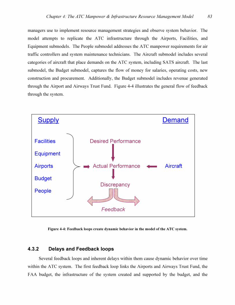
Chapter 4: The ATC Manpower & Infrastructure Resource Management Model 83
managers use to implement resource management strategies and observe system behavior. The
model attempts to replicate the ATC infrastructure through the Airports, Facilities, and
Equipment submodels. The People submodel addresses the ATC manpower requirements for air
traffic controllers and system maintenance technicians. The Aircraft submodel includes several
categories of aircraft that place demands on the ATC system, including SATS aircraft. The last
submodel, the Budget submodel, captures the flow of money for salaries, operating costs, new
construction and procurement. Additionally, the Budget submodel includes revenue generated
through the Airport and Airways Trust Fund. Figure 4-4 illustrates the general flow of feedback
through the system.
Figure 4-4: Feedback loops create dynamic behavior in the model of the ATC system.
4.3.2 Delays and Feedback loops
Several feedback loops and inherent delays within them cause dynamic behavior over time
within the ATC system. The first feedback loop links the Airports and Airways Trust Fund, the
FAA budget, the infrastructure of the system created and supported by the budget, and the
Supply Demand
Facilities Desired Performance Equipment Airports Actual Performance Aircraft Budget Discrepancy People
Feedback

Chapter 4: The ATC Manpower & Infrastructure Resource Management Model 84
aircraft the system can support. Ultimately, the number of aircraft supported generates revenue
that feeds into the trust fund to reinforce the operation of the ATC system. Several feedback
loops connect the submodels and cause internal adjustments among the stocks in the submodels.
Delays occur in some loops, such as the requirement to train controllers and maintainers before
they can become fully qualified. The interaction of the feedback loops and the delays causes
growth, decay, or oscillations in the system performance metrics.
4.3.3 Modeling Assumptions
The following assumptions simplify and shape the model structure, while still capturing the
essential aspects of the real world system.
1. The core of the current national airspace system will evolve with technology, but remain
fundamentally the same. Thus, the air carrier aircraft will continue to function in a
system primarily controlled by human controllers in a system of control towers,
TRACONs, and ARTCCs.
2. The peripheral parts of the national airspace system will be the areas subject to the most
change. The thousands of small airports around the country that do not connect to the
hub and spoke system will provide the most opportunity to support SATS aircraft through
the application of new GPS-based technology.
3. Two Air Route Traffic Control Centers will consolidate into one center in 2010.
ARTCCs will perform monitoring roles under GPS-based ATC architectures in addition
to their radar-based ATC responsibilities.
4. All Flight Service Stations will also perform monitoring roles under GPS-based ATC
architectures.
5. The ATC community will resolve future airspace issues that may interfere with SATS
operations.
6. The FAA will continue to experience budget trends like those of the past. However, the
model will capture dynamic system feedback through the Airport and Airways Trust
Fund.
7. Projections from the FAA regarding aircraft growth rates will serve as a basis for similar
parameters in the model, which are listed in Table 5-2.
Chapter 4: The ATC Manpower & Infrastructure Resource Management Model 85
8. The ATC system will not allow for mixed modes of traffic operating within the same
airspace. Aircraft will fly according to IFR, VFR, or in accordance with “SATS flight
rules.”
9. Military aircraft will adjust their use of Public Use Airports to accommodate the growth
of SATS airports.
4.3.4 Modeling Objectives
The objective of the modeling effort is to present a top-level System Dynamics model of
the ATC system that shows the cause and effect relationships among the “supply” of ATC
services provided by facilities, equipment, manpower, airports and the budget; and the “demand”
for ATC services from aircraft. Additionally, the modeling effort should replicate the current
ATC system and project its behavior into the future based upon various resource management
strategies that may change the system structure. Finally, the model should demonstrate the
potential support the ATC system may provide to the future SATS and subsequent behavior of
the system under the influence of SATS aircraft. Users of the model will see how the various
resource management strategies of the ATC system will dynamically behave over time.
4.4 Modeling ATC Resource Management Strategies
The model is useful to investigate three strategies FAA managers may pursue. The three
strategies involve policies to meet the demand for ATC instrument operations from conventional
aircraft and to expand the growth of systems to support GPS-based ATC. The GPS-based ATC
will be the primary means by which SATS aircraft will navigate and maintain separation from
other aircraft. The model will also provide an indication of the amount of SATS flights the ATC
system will support under the various resource management strategies and the revenue produced
by the system.
4.4.1 Strategy 1: Maintain the Radar-based System
The first strategy is to maintain the current ATC system by investing in people, airports,
facilities, and equipment to meet the demands of aircraft operating under radar-based ATC. The
primary objective of resource managers using the first strategy is to continue to expand and
modernize the radar-based ATC system. Most resources will go to achieving that goal.
Chapter 4: The ATC Manpower & Infrastructure Resource Management Model 86
However, some resources will support a low level of GPS-based ATC growth as part of the
system modernization effort.
4.4.2 Strategy 2: Reduce the Radar-based System
The second strategy is to aggressively reduce the radar-based ATC system by
maintaining a high rate of investment in GPS-based ATC equipment and airports while accepting
shortfalls in the radar-based ATC system during the transition period. Conceptually, the strategy
would induce delays in the radar-based system and cause aircraft owners to invest in on-board
systems to operate in the GPS-based environment.
4.4.3 Strategy 3: Supplement the Radar-based System
The third strategy is to supplement the radar-based ATC system with a GPS-based ATC
system growing at a rate that is constrained somewhat by the requirements of the radar-based
ATC system. Managers would provide resources to meet the demand for radar-based ATC while
using all additional funding to expand the GPS-based system.
4.4.4 ATC Resource Management Policies
Strategies are combinations of policies. The above three strategies consist of
combinations of two FAA resource management policies. The first policy determines the desired
level of support the FAA should attempt to give to aircraft that demand radar-based ATC
services. The amount of money devoted to the accounts that pay for the radar-based ATC
services is a surrogate measure of the level of support. Since resource management is a zero sum
game, managers would direct the money not devoted to radar-based ATC toward GPS-based
ATC requirements. The second policy determines the timeframe over which resource managers
should implement the first policy. The timeframe consists of a period of years bounded by a start
year, a period of adjustment, and a target year in which the first policy would be in full effect.
The combination of policies one and two create three exogenous decision variables for the
system: a target level of radar-based ATC funding, a year to begin transitioning to the desired
new funding level, and an end year to fully meet the funding objective.

Chapter 4: The ATC Manpower & Infrastructure Resource Management Model 87
4.4.5 Exogenous Input into the System and the Model
The model boundary diagram in Figure 4-5 distinguishes between endogenous and
exogenous components of the system and the outside world excluded from the model. The
endogenous components include the stocks and flows within the system that, if unperturbed by
outside forces, create normal system behavior. The exogenous components include the aspects
of the system that generally remain constant over time and influence the endogenous parts of the
system. Resource managers will utilize funding levels for radar-based or GPS-based airports,
equipment, and facilities to influence the behavior of the ATC system. It is desirable to
minimize the impact of other potential exogenous inputs into the model to limit the behavior of
the model to the internal structure of the system and those management controlled external
variables. The excluded aspects of the outside world provide a sense of the domain represented
by the model.
Figure 4-5: The model boundary diagram conveys the domain of the modeling effort.
FAA Budget Accounts
Facilities
Equipment
US Economy
Airports
CongressTechnology
Flights
Resource Management Strategy
Alternate sources of transportation
Fuel Prices
ENDOGENOUS
EXOGENOUS
EXCLUDED
People
Grants in
Aid
Chapter 4: The ATC Manpower & Infrastructure Resource Management Model 88
4.5 Model subsystems
The model consists of six subsystems that work together to replicate the flow of resources
through the ATC system in the US. The People Subsystem includes air traffic controllers and
field maintenance personnel. The Budget Subsystem includes the FAA annual budget as well as
the Airport and Airways Trust Fund. The Facilities Subsystem includes Air Route Traffic
Control Centers, Terminal Area Controls, Air Traffic Control Towers, and Flight Service
Stations. The Equipment Subsystem includes equipment that supports radar-based or GPS-based
ATC. The Airports Subsystem includes non-SATS and SATS airports. The Aircraft Subsystem
includes commercial airliners, air taxi, general aviation, and SATS aircraft. Decision-making
occurs when stocks change. The decisions create dynamic endogenous feedback in the system
that causes further changes in the stocks and flows. The exogenous input in the form of resource
management strategies generates dynamic behavior that provides insight into the potential
system performance generated by the interaction of the subsystems.
The remainder of Chapter 4 provides the details of the subsystems that combine to create
the ATC manpower and infrastructure resource management model. Each subsystem includes a
written description, additional diagrams, equations, tables, and explanations regarding the
development of model parameters.
4.6 The People Subsystem
The people subsystem consists of the 50,000 employees of the FAA. Table 4-1 below
shows the distribution of employees throughout the FAA. Over 85% of the people in the FAA
work in two main areas: Air Traffic Services, and, Regulation and Certification. Within Air
Traffic Services there are approximately 17,500 air traffic controllers, 8,500 field maintenance
personnel, 3,000 Flight Service Station employees, and 6,000 employees involved in
telecommunications, logistics, or system requirements. Within Regulation and Certification
there are approximately 4,000 inspectors, engineers, and pilots; 1,000 technical and field support
personnel and 700 employees involved in certification administration, aviation safety education,
and research (FAA, 2001b). The Civil Aviation Security organization, which consisted of about
1,200 FAA employees, transferred to the newly formed Transportation Security Administration
in the wake of the events of September 11, 2001.

Chapter 4: The ATC Manpower & Infrastructure Resource Management Model 89
The number of people in the ATC system influences the amount of money Congress must
provide for the FAA budget. Historically, the AATF provided from 34% to 100% of the money
needed for employee salaries and benefits. Primarily, the AATF provides money for
improvements to airports and modernization of facilities and equipment. In the FAA budget and
in the model, Congress must make up for shortfalls in the budget not provided for by the AATF.
The challenge in modeling the people subsystem lies in the determination of how future
technology will impact upon the need for people in the system. The people subsystem model
uses aircraft, facilities and equipment, and ATC technology growth rates combined with
manpower requirements from policy decisions to determine how the behavior of the system will
influence the need for FAA employees.
Table 4-1: The FAA employs approximately 50,000 people.
FAA Employees 1996 1997 1998 1999 2000 2001 2002 (est)
Air Traffic Services 34,929 35,019 35,789 35,732 35,425 36,349 36,216Regulation and Certification
5,132 5,766 5,721 6,030 5,864 6,195 6,122
Civil Aviation Security 755 1,015 1,175 1,156 1,153 1,221 0Airports 463 472 483 490 446 472 464Research and Acquisitions
777 770 1,899 1,902 1,898 1,858 1,850
Comm Space Transportation
28 34 28 30 25 44 60
Staff Offices & Other 5,211 5,190 3,704 3,728 3,652 3,762 3,794Total 47,295 48,266 48,799 49,068 48,463 49,901 48,506
Source: FAA, 2002a
Table 4-2 provides a breakdown of the distribution of employees among the Air Traffic
Services and Regulation and Certification components of the FAA, where the majority of FAA
employees work.
Table 4-2: Approximately 85% of FAA employees work in either Air Traffic Services or Regulation and
Certification.
ATS and R&C Employees
1998 1999 2000 2001 2002 (est)
Air Traffic Controllers 17,756 17,639 17,547 17,510 17,464Field Maintenance 8,338 8,070 7,830 8,188 8,493Flight Service Stations 3,100 3,017 2,976 2,934 2,872Other ATS 6,595 7,006 7,072 7,717 7,387Inspectors, Engineers, Pilots (Flt Standards) 4,506 4,357 4,206 4,476 4,407
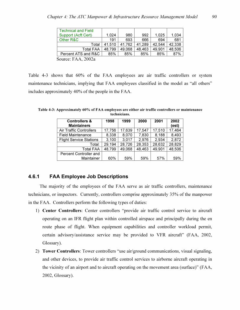
Chapter 4: The ATC Manpower & Infrastructure Resource Management Model 90
Technical and Field Support (Acft Cert) 1,024 980 992 1,025 1,034Other R&C 191 693 666 694 681
Total 41,510 41,762 41,289 42,544 42,338Total FAA 48,799 49,068 48,463 49,901 48,506
Percent ATS and R&C 85% 85% 85% 85% 87%
Source: FAA, 2002a
Table 4-3 shows that 60% of the FAA employees are air traffic controllers or system
maintenance technicians, implying that FAA employees classified in the model as “all others”
includes approximately 40% of the people in the FAA.
Table 4-3: Approximately 60% of FAA employees are either air traffic controllers or maintenance
technicians.
Controllers & Maintainers
1998 1999 2000 2001 2002 (est)
Air Traffic Controllers 17,756 17,639 17,547 17,510 17,464Field Maintenance 8,338 8,070 7,830 8,188 8,493Flight Service Stations 3,100 3,017 2,976 2,934 2,872
Total: 29,194 28,726 28,353 28,632 28,829Total FAA 48,799 49,068 48,463 49,901 48,506
Percent Controller and Maintainer 60% 59% 59% 57% 59%
4.6.1 FAA Employee Job Descriptions
The majority of the employees of the FAA serve as air traffic controllers, maintenance
technicians, or inspectors. Currently, controllers comprise approximately 35% of the manpower
in the FAA. Controllers perform the following types of duties:
1) Center Controllers: Center controllers “provide air traffic control service to aircraft
operating on an IFR flight plan within controlled airspace and principally during the en
route phase of flight. When equipment capabilities and controller workload permit,
certain advisory/assistance service may be provided to VFR aircraft” (FAA, 2002,
Glossary).
2) Tower Controllers: Tower controllers “use air/ground communications, visual signaling,
and other devices, to provide air traffic control services to airborne aircraft operating in
the vicinity of an airport and to aircraft operating on the movement area (surface)” (FAA,
2002, Glossary).
Chapter 4: The ATC Manpower & Infrastructure Resource Management Model 91
3) Approach Controllers: Approach controllers “use radar and air/ground communications
to provide approach control services to aircraft arriving, departing, or transiting the
airspace controlled by the facility” (FAA, 2002, Glossary).
4) Automated Flight Service Stations and Flight Service Station Controllers:
Controllers at FSSs and AFSSs, “provide preflight pilot briefings and en route
communications with VFR flights, assist lost aircraft, assist aircraft having emergencies,
relay air traffic control clearances, originate, classify, and disseminate Notices to Airmen,
broadcast aviation weather and national airspace system information, receive and close
flight plans, monitor radio navigational aids, notify search and rescue units of missing
VFR aircraft and operate the national weather teletypewriter systems. In addition, at
selected locations, FSS controllers take weather observations, issue airport advisories,
administer airmen written examinations, and advise Customs & Immigration of
transborder flights” (FAA, 2002, Glossary).
Many FAA employees serve as maintainers and inspectors:
1) Airway Transportation Systems Specialists and Electronics Technicians: The FAA
employs Airway Transportation Systems Specialists and Electronics Technicians to
design, develop, install, certify, inspect, and repair thousands of pieces of equipment in or
near airports and at remote sites to support the ATC mission. The maintenance
specialists and technicians work with equipment such as radar, computers,
communications, navigational aids, lighting aids, and the mechanical and electrical
components of FAA facilities.
2) Aviation Safety Inspectors: The FAA employs Aviation Safety Inspectors to ensure that
those who produce, maintain, operate, and modify civil aircraft comply with all
applicable standards and regulations.
4.6.2 Modeling the People Subsystem
The model treats FAA employees as entities in the system and places them into three
categories: controllers, maintainers, or all others. Both the controllers and maintainers occupy
two stocks each. The model treats all other employees as a function of the number of controllers
and maintainers. Over time, employees flow into the stocks as new hires and eventually leave
the system as retirees. Several assumptions underlie the people subsystem model:
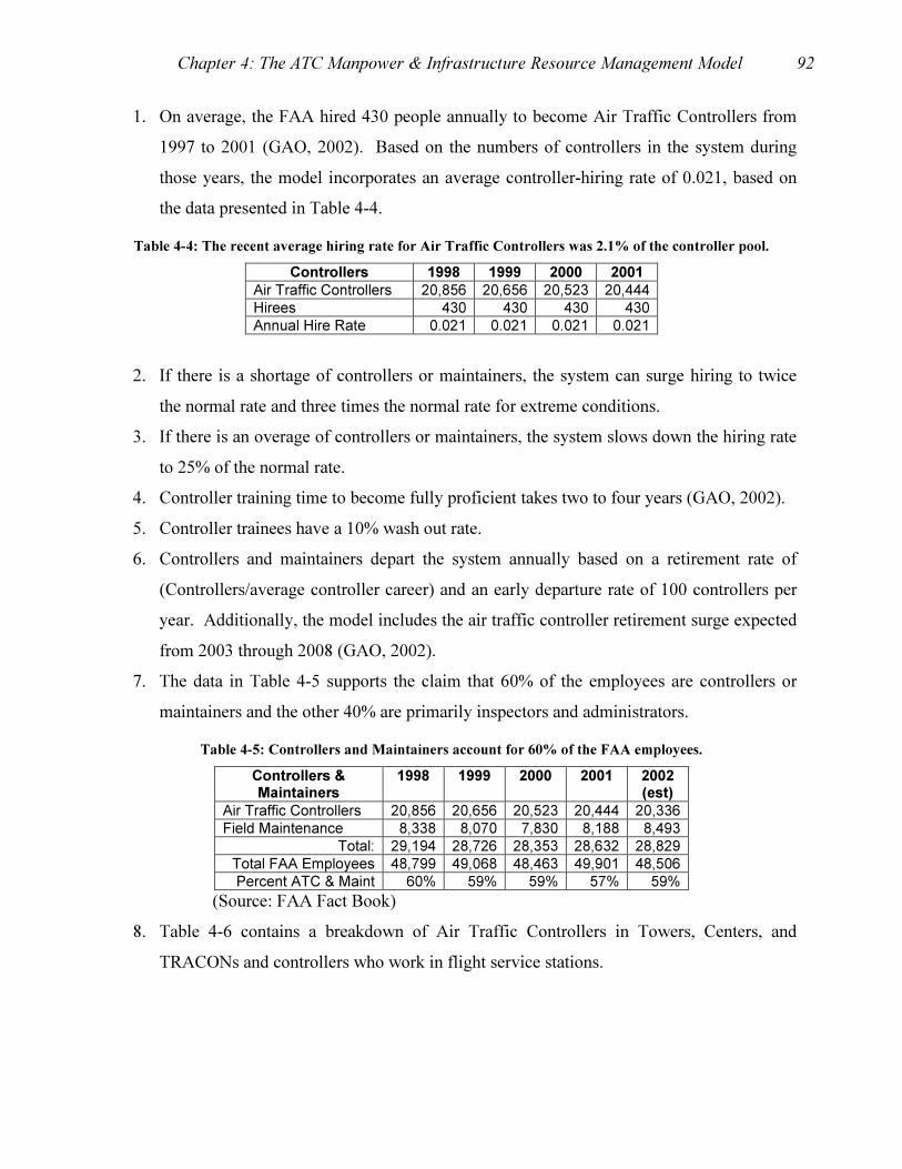
Chapter 4: The ATC Manpower & Infrastructure Resource Management Model 92
1. On average, the FAA hired 430 people annually to become Air Traffic Controllers from
1997 to 2001 (GAO, 2002). Based on the numbers of controllers in the system during
those years, the model incorporates an average controller-hiring rate of 0.021, based on
the data presented in Table 4-4.
Table 4-4: The recent average hiring rate for Air Traffic Controllers was 2.1% of the controller pool.
Controllers 1998 1999 2000 2001 Air Traffic Controllers 20,856 20,656 20,523 20,444 Hirees 430 430 430 430 Annual Hire Rate 0.021 0.021 0.021 0.021
2. If there is a shortage of controllers or maintainers, the system can surge hiring to twice
the normal rate and three times the normal rate for extreme conditions.
3. If there is an overage of controllers or maintainers, the system slows down the hiring rate
to 25% of the normal rate.
4. Controller training time to become fully proficient takes two to four years (GAO, 2002).
5. Controller trainees have a 10% wash out rate.
6. Controllers and maintainers depart the system annually based on a retirement rate of
(Controllers/average controller career) and an early departure rate of 100 controllers per
year. Additionally, the model includes the air traffic controller retirement surge expected
from 2003 through 2008 (GAO, 2002).
7. The data in Table 4-5 supports the claim that 60% of the employees are controllers or
maintainers and the other 40% are primarily inspectors and administrators.
Table 4-5: Controllers and Maintainers account for 60% of the FAA employees.
Controllers & Maintainers
1998 1999 2000 2001 2002 (est)
Air Traffic Controllers 20,856 20,656 20,523 20,444 20,336Field Maintenance 8,338 8,070 7,830 8,188 8,493
Total: 29,194 28,726 28,353 28,632 28,829Total FAA Employees 48,799 49,068 48,463 49,901 48,506Percent ATC & Maint 60% 59% 59% 57% 59%
(Source: FAA Fact Book)
8. Table 4-6 contains a breakdown of Air Traffic Controllers in Towers, Centers, and
TRACONs and controllers who work in flight service stations.

Chapter 4: The ATC Manpower & Infrastructure Resource Management Model 93
Table 4-6: Approximately 42% of all FAA employees are air traffic controllers.
Controllers 1998 1999 2000 2001 2002 (est)
Air Traffic Controllers 17,756 17,639 17,547 17,510 17,464Flight Service Stations 3,100 3,017 2,976 2,934 2,872
Total: 20,856 20,656 20,523 20,444 20,336Total FAA 48,799 49,068 48,463 49,901 48,506
Percent 43% 42% 42% 41% 42%
(Source: FAA Fact Book)
9. The number of facilities in the system determines the total number of controllers, as
depicted in Table 4-7.
Table 4-7: Estimates of the number of controllers per facility.
Type Facility 1998 Avg # Controllers
Total Controllers
Centers 21 375 7,875
Core AC Towers 170 18 3,060
Core AT Towers 135 8 1,080
Core GA Towers 157 5 785
Approach Controls 190 25 4,750
FSS/AFSS 137 22 2,992
Total: 20,542
(Source: FAA Fact Book)
10. The amount of equipment in the system and the number of controllers determines how
many maintainers are in the system. Table 4-8 shows that there are approximately 1.09
maintainers per piece of radar-based equipment in the ATC system. The model includes
assumptions that the same maintainer to equipment ratio will apply to GPS-based ATC
equipment. Table 4-9 contains data to support the assumption that the average ratio of
0.40 field maintenance personnel to air traffic controllers provides an estimation of how
many maintainers work in the ATC system.
Table 4-8: There are approximately 1.09 maintainers for each piece of equipment in the ATC system.
Maintainers 1998 1999 Field Maintenance 8,338 8,070Radar-based Eqpt 7,460 7,685Ratio 1.12 1.05
(Source: FAA Budget in Brief, 2001)

Chapter 4: The ATC Manpower & Infrastructure Resource Management Model 94
Table 4-9: There are approximately 0.4 maintainers for each controller in the ATC system.
Controllers to Maintainers Ratio
1998 1999 2000 2001 2002 (est)
Field Maintenance 8,338 8,070 7,830 8,188 8,493Air Traffic Controllers 20,856 20,656 20,523 20,444 20,336Ratio 0.40 0.39 0.38 0.40 0.42
(Source: FAA Fact Book)
11. Model calculations determine the required number of maintainers by taking the average
of 0.4*(controllers) and 1.09*(radar-based equipment + GPS-based equipment).
12. The number of controllers and maintainers determines the number of “all other”
employees in the system. As suggested in Table 4-5 above, all other employees account
for 40% of the FAA workforce.
4.6.3 People Subsystem Stock & Flow Diagrams
The controller and maintainer stock and flow diagrams in Figure 4-6 and Figure 4-7
include the assumptions and descriptions discussed above.
Controllerscontroller retire
rate
avg controllers per
center
<Centers>
required
controllers
controller
discrepancy
controller hiring
function
effect of controllerdiscrepancy on hiring
rate
normal controller
hiring rate
controller retiring
function
effect of controllerdiscrepancy on retiring
rate
average controller
career
percent
controllers hired
avg controllers per
AC tower
avg controllers per
TRACONavg controllers
per FSS<AC
Towers><TRACONs>
<FSSs>
early depart rate
Controller
Traineesnew controllerscontroller hire rate
trainee training
time
wash out
normal wash
out
controller retirement
surge 2003 to 2008
retirees per surge
year
<AT Towers>
<GA Towers>
avg controllers per
GA tower
avg controllers per
AT tower
min shortfall ctrl
hire rate
<effect of budget
ratio>
delayed
retirements
Figure 4-6: The controller stock and flow diagram.

Chapter 4: The ATC Manpower & Infrastructure Resource Management Model 95
Maintainers
maintainer retire
rate
normal maintainer
hiring rate
average maintainer
career
required
maintainers
<Controllers>
<Radar based
Equipment>
average maintainers
per controlleraverage maintainers
per equipment
<GPS based
Equipment>
maintainer
discrepancy
maintainer hiring
function
effect of maintainerdiscrepancy on hiring
rate
maintainer retiring
function
effect of maintainerdiscrepancy on retiring
rate
Maintainer
Trainees new maintainersmaintainer hire rate
maintainer trainee
training timeaccelerated retirement
due to average age
effect of accelerated
retirement
start of accelerated
retirement
<time period>
<effect of budget
ratio>
Figure 4-7: The maintainer stock and flow diagram.
4.7 The FAA Budget Subsystem
Resources that ATC managers use to purchase new infrastructure and pay employees
reside in the FAA Budget subsystem. The Budget subsystem consists of both income and
expenditures. The FAA generates revenue from excise taxes collected for the Airports and
Airways Trust Fund. The FAA budget consists of four major components: Operations, Facilities
and Equipment, Grants-in-Aid for Airports, and Research and Development. The FAA Budget
submodel includes the Research and Development account as an amount equal to 2% of the FAA
budget.
Within the FAA budget subsystem, management resource allocation decisions direct the
funding for airports, facilities, and navigation equipment. The infrastructure created, maintained,
and modernized through the resource allocation process influences the number of people needed
to provide and maintain ATC services. Subsequently, the cost of employees and the operating
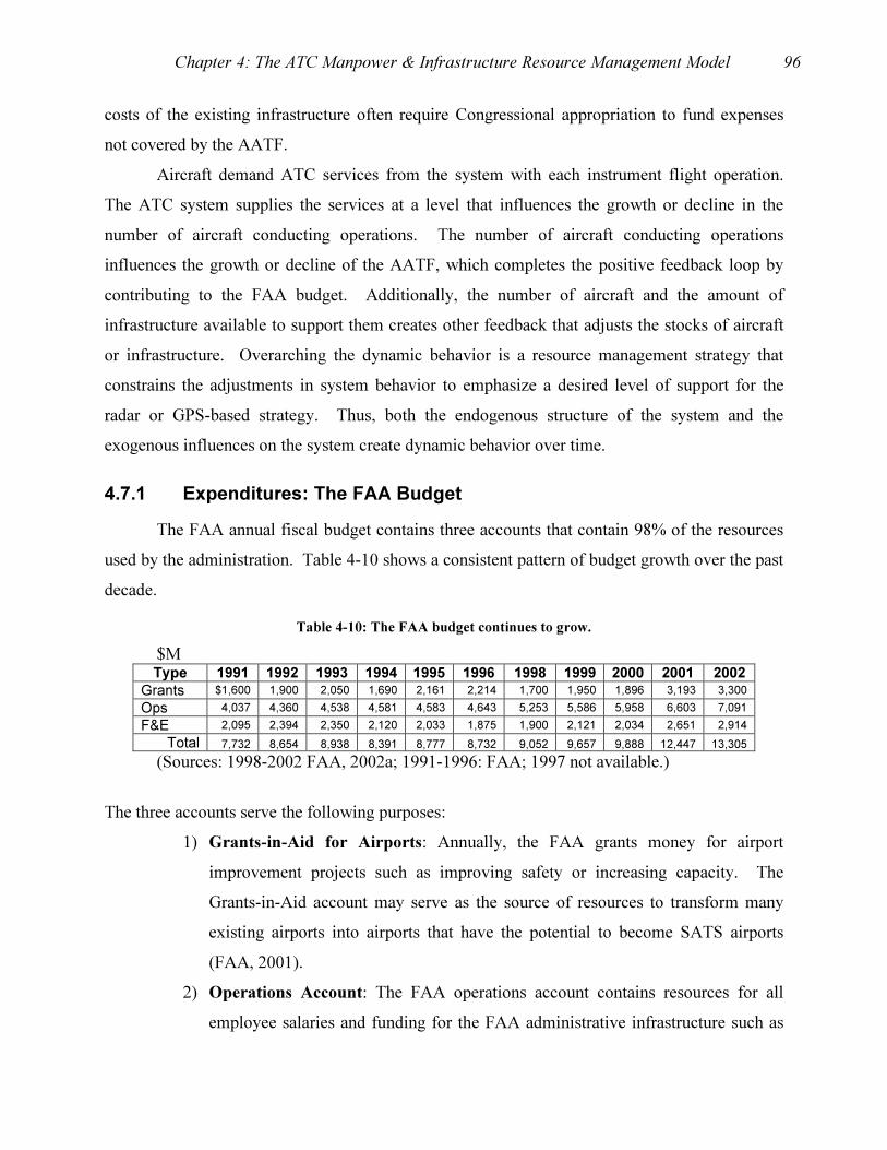
Chapter 4: The ATC Manpower & Infrastructure Resource Management Model 96
costs of the existing infrastructure often require Congressional appropriation to fund expenses
not covered by the AATF.
Aircraft demand ATC services from the system with each instrument flight operation.
The ATC system supplies the services at a level that influences the growth or decline in the
number of aircraft conducting operations. The number of aircraft conducting operations
influences the growth or decline of the AATF, which completes the positive feedback loop by
contributing to the FAA budget. Additionally, the number of aircraft and the amount of
infrastructure available to support them creates other feedback that adjusts the stocks of aircraft
or infrastructure. Overarching the dynamic behavior is a resource management strategy that
constrains the adjustments in system behavior to emphasize a desired level of support for the
radar or GPS-based strategy. Thus, both the endogenous structure of the system and the
exogenous influences on the system create dynamic behavior over time.
4.7.1 Expenditures: The FAA Budget
The FAA annual fiscal budget contains three accounts that contain 98% of the resources
used by the administration. Table 4-10 shows a consistent pattern of budget growth over the past
decade.
Table 4-10: The FAA budget continues to grow.
$M Type 1991 1992 1993 1994 1995 1996 1998 1999 2000 2001 2002
Grants $1,600 1,900 2,050 1,690 2,161 2,214 1,700 1,950 1,896 3,193 3,300
Ops 4,037 4,360 4,538 4,581 4,583 4,643 5,253 5,586 5,958 6,603 7,091
F&E 2,095 2,394 2,350 2,120 2,033 1,875 1,900 2,121 2,034 2,651 2,914
Total 7,732 8,654 8,938 8,391 8,777 8,732 9,052 9,657 9,888 12,447 13,305
(Sources: 1998-2002 FAA, 2002a; 1991-1996: FAA; 1997 not available.)
The three accounts serve the following purposes:
1) Grants-in-Aid for Airports: Annually, the FAA grants money for airport
improvement projects such as improving safety or increasing capacity. The
Grants-in-Aid account may serve as the source of resources to transform many
existing airports into airports that have the potential to become SATS airports
(FAA, 2001).
2) Operations Account: The FAA operations account contains resources for all
employee salaries and funding for the FAA administrative infrastructure such as
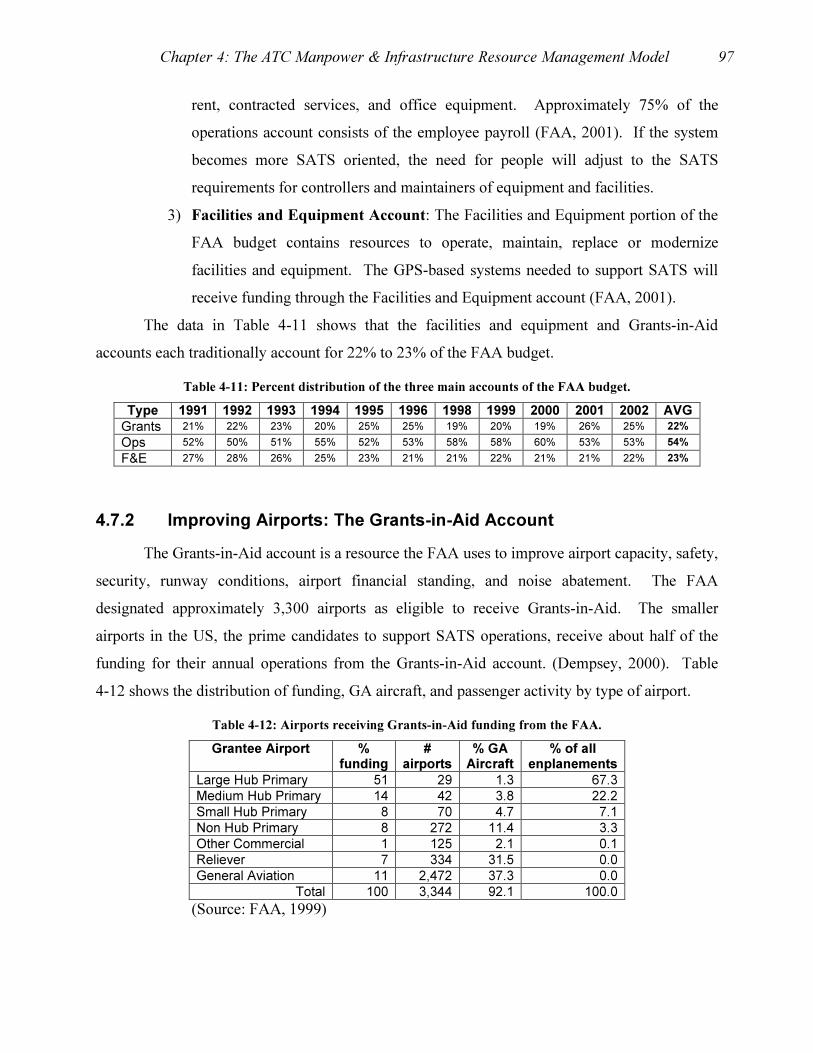
Chapter 4: The ATC Manpower & Infrastructure Resource Management Model 97
rent, contracted services, and office equipment. Approximately 75% of the
operations account consists of the employee payroll (FAA, 2001). If the system
becomes more SATS oriented, the need for people will adjust to the SATS
requirements for controllers and maintainers of equipment and facilities.
3) Facilities and Equipment Account: The Facilities and Equipment portion of the
FAA budget contains resources to operate, maintain, replace or modernize
facilities and equipment. The GPS-based systems needed to support SATS will
receive funding through the Facilities and Equipment account (FAA, 2001).
The data in Table 4-11 shows that the facilities and equipment and Grants-in-Aid
accounts each traditionally account for 22% to 23% of the FAA budget.
Table 4-11: Percent distribution of the three main accounts of the FAA budget.
Type 1991 1992 1993 1994 1995 1996 1998 1999 2000 2001 2002 AVG Grants 21% 22% 23% 20% 25% 25% 19% 20% 19% 26% 25% 22%
Ops 52% 50% 51% 55% 52% 53% 58% 58% 60% 53% 53% 54%
F&E 27% 28% 26% 25% 23% 21% 21% 22% 21% 21% 22% 23%
4.7.2 Improving Airports: The Grants-in-Aid Account
The Grants-in-Aid account is a resource the FAA uses to improve airport capacity, safety,
security, runway conditions, airport financial standing, and noise abatement. The FAA
designated approximately 3,300 airports as eligible to receive Grants-in-Aid. The smaller
airports in the US, the prime candidates to support SATS operations, receive about half of the
funding for their annual operations from the Grants-in-Aid account. (Dempsey, 2000). Table
4-12 shows the distribution of funding, GA aircraft, and passenger activity by type of airport.
Table 4-12: Airports receiving Grants-in-Aid funding from the FAA.
Grantee Airport % funding
# airports
% GA Aircraft
% of all enplanements
Large Hub Primary 51 29 1.3 67.3 Medium Hub Primary 14 42 3.8 22.2 Small Hub Primary 8 70 4.7 7.1 Non Hub Primary 8 272 11.4 3.3 Other Commercial 1 125 2.1 0.1 Reliever 7 334 31.5 0.0 General Aviation 11 2,472 37.3 0.0
Total 100 3,344 92.1 100.0
(Source: FAA, 1999)
Chapter 4: The ATC Manpower & Infrastructure Resource Management Model 98
The 413 public use primary airports, serving as large, medium, small, and non-hub
airports, receive a minimum of $500,000 annually in FAA Grants-in-Aid. The FAA determines
the maximum amount based on number of enplanements. Large hub airports each support at
least 1% of all US enplanements. Medium hubs enplane between 0.25% and 1% of all
enplanements. Small hubs enplane between 0.05% and 0.25%. Non Hub primary airports
enplane less than 0.05% of all enplanements, but exceed 10,000 enplanements annually. All
other commercial service airports have at least 2,500 to 10,000 enplanements annually, but
altogether only account for 0.1% of all US enplanements. Reliever airports provide GA aircraft
with easy and inexpensive access to congested metropolitan areas. Usually, at least one General
Aviation airport exists in each county in rural areas throughout the US.
The FAA uses the National Plan of Integrated Airport Systems (NPIAS) as the document
that captures local, state, and regional airport capital improvement planning. The FAA
distributes money through the Airport Improvement Program to fund one quarter to one third of
all capital improvement projects at US public use airports initially identified in the NPIAS (FAA,
2001b). The NPIAS is a five-year forecast that includes a list of 3,334 US public use airports
that require more than $35B of capital improvement. The capital projects consist primarily to
improve safety, capacity, noise abatement, runway pavement, financial performance, and ground
accessibility to airports. Future security improvement requirements will most likely increase as a
result of the terrorist attacks of 2001. Air traffic control navigation facilities and equipment do
not fall under the Airport Improvement Program, but rather receive funding through the facilities
and equipment account of the FAA budget (DOT, 1999).
Although most SATS airport development efforts will involve navigation and approach
systems, SATS airports may need to compete for AIP funding to make them fully operational.
For example, almost 2,000 of the potential SATS airports have unpaved landing areas. The
source of AIP funding will be the FAA Grants-in Aid account, which the data from Table 4-10
shows to be growing at a rate of $120M annually from 1991 to 2002 or $444M annually from
1998 to 2002. The model uses an annual growth rate of $170M for the Grants-in-Aid account.
Most NPIAS projects take place at airports supporting commercial air carriers. Data in
the “% funding” column of Table 4-12 shows that only 18% of the $35B project plans address
needs at General Aviation and Reliever airports that are the most likely candidates to become
SATS airports. Only 1% of the $35B would go to construction of new airports. The primary

Chapter 4: The ATC Manpower & Infrastructure Resource Management Model 99
purposes of the projects are to add capacity and bring existing airports up to acceptable
standards. There are approximately 2,000 public use airports absent from the NPIAS list because
they have low activity, are within 20 miles of an NPIAS airport, or are unsuitable for further
expansion. Although NASA claims these may be suitable SATS airports, the model only
recognizes the 3,344 NPIAS airports as potential SATS airports.
4.7.3 Supporting People: The Operations Account
The operations account is the largest of the three major accounts in the FAA budget. The
operations account includes more than half of the FAA fiscal resources. Table 4-13 contains a
breakdown of all the categories of expenditures in the operations account. Table 4-13 shows that
the FAA abolished the “Airports” and “Administration” accounts in 2000, transferred some of
the funding to Research and Acquisition and also replaced them with the new accounts
“Regions/Centers Operations, Human Resources,” and “Financial Services” (FAA, 2001).
However, as seen in Table 4-14, the abolished and new accounts only comprise about 6% of the
FAA budget.
Table 4-13: Distribution of funding in the Operations Account.
Operations 1998 $M
1999 2000 2001 2002 2003 (est)
Air Traffic Services $4,080 4,351 4,670 5,446 5,792 6,096 Regulation and Certification
600 619 645 735 810 839
Civil Aviation Security 115 120 136 150 179 9 Research and Acquisitions 93 78 174 193 199 206 Commercial Space Transportation 6 6 6 12 12 12 Regions/Centers Operations NR NR 85 103 92 95 Human Resources NR NR 66 57 72 74 Financial Services NR NR 40 49 51 53 Staff Offices 76 84 76 109 114 113 Emergency Response Fund NR NR 0 1 473 0 Information Services NR NR 0 0 0 5 Airports 48 48 NR NR NR NR Administration 260 264 NR NR NR NR
Total 5,277 5,570 5,898 6,855 7,794 7,502
NR = Not Reported; Source: FAA, 2002a
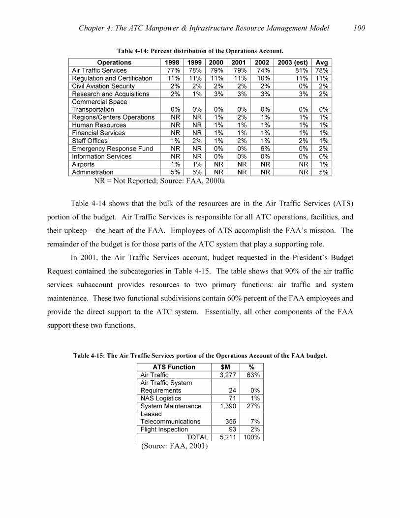
Chapter 4: The ATC Manpower & Infrastructure Resource Management Model 100
Table 4-14: Percent distribution of the Operations Account.
Operations 1998 1999 2000 2001 2002 2003 (est) Avg Air Traffic Services 77% 78% 79% 79% 74% 81% 78% Regulation and Certification 11% 11% 11% 11% 10% 11% 11% Civil Aviation Security 2% 2% 2% 2% 2% 0% 2% Research and Acquisitions 2% 1% 3% 3% 3% 3% 2% Commercial Space Transportation 0% 0% 0% 0% 0% 0% 0% Regions/Centers Operations NR NR 1% 2% 1% 1% 1% Human Resources NR NR 1% 1% 1% 1% 1% Financial Services NR NR 1% 1% 1% 1% 1% Staff Offices 1% 2% 1% 2% 1% 2% 1% Emergency Response Fund NR NR 0% 0% 6% 0% 2% Information Services NR NR 0% 0% 0% 0% 0% Airports 1% 1% NR NR NR NR 1% Administration 5% 5% NR NR NR NR 5%
NR = Not Reported; Source: FAA, 2000a
Table 4-14 shows that the bulk of the resources are in the Air Traffic Services (ATS)
portion of the budget. Air Traffic Services is responsible for all ATC operations, facilities, and
their upkeep – the heart of the FAA. Employees of ATS accomplish the FAA’s mission. The
remainder of the budget is for those parts of the ATC system that play a supporting role.
In 2001, the Air Traffic Services account, budget requested in the President’s Budget
Request contained the subcategories in Table 4-15. The table shows that 90% of the air traffic
services subaccount provides resources to two primary functions: air traffic and system
maintenance. These two functional subdivisions contain 60% percent of the FAA employees and
provide the direct support to the ATC system. Essentially, all other components of the FAA
support these two functions.
Table 4-15: The Air Traffic Services portion of the Operations Account of the FAA budget.
ATS Function $M % Air Traffic 3,277 63% Air Traffic System Requirements 24 0% NAS Logistics 71 1% System Maintenance 1,390 27% Leased Telecommunications 356 7% Flight Inspection 93 2%
TOTAL 5,211 100%
(Source: FAA, 2001)

Chapter 4: The ATC Manpower & Infrastructure Resource Management Model 101
The data in Table 4-16 shows that Payroll accounted for approximately 74% of the
Operations account, which implies that payroll was 40% of the FAA’s entire budget in 2001.
Subsequently, an assumption built into the model is that 26% of the operations account is for
contracts, services, rent, and travel related to the employees. Within the model, the initial
distribution of funds from the operations account pays for employee salaries and the additional
services. After paying for salaries and services, the model uses the remainder of the FAA budget
to build facilities or purchase equipment as directed by the resource management strategy and the
feedback from the system.
Table 4-16: The Operations Account pays for salaries and services.
Operations $M % Payroll 4,861 74% Contracts & Other Services 838 13% Rent & Utilities 506 8% Equipment & Supplies 256 4% Travel & Transportation 131 2%
TOTAL 6,592 101%
Source: FAA, 2001
The 2001 President’s Budget request also subdivided the Air Traffic Services (ATS)
budget according to the six functional suborganizations in Table 4-17. The data in the table
indicates that the preponderance of resources supports air traffic control and maintenance of the
ATC system.
Table 4-17: Functional subdivisions of the Air Traffic Services account.
ATS Suborganizations
$ %
Air Traffic 3,277 63% Air Traffic System Requirements Service 24 0% NAS Logistics 71 1% Systems Maintenance 1,390 27% Leased Telecommunications 356 7% Flight Inspection and Procedures 93 2%
TOTAL 5,211
Source: FAA, 2001
Chapter 4: The ATC Manpower & Infrastructure Resource Management Model 102
1) Air Traffic: The Air Traffic subactivity of the ATS component of the FAA is responsible
for the safe and efficient control of aircraft all day, every day. Air Traffic operates 21 en
route centers, 437 control towers, 190 TRACONs, and 137 Flight Service Stations.
2) Air Traffic System Requirements Service: The requirements subactivity manages the
processes for determining and fulfilling the immediate and future operational needs of
Air Traffic Services.
3) NAS Logistics: The logistics subactivity procures equipment, land, and office space;
provides spare parts; conducts limited maintenance; and manages the Mike Munroney
Aeronautical Center.
4) Systems Maintenance: The maintenance subactivity maintains and repairs all FAA
facilities and equipment such as navigation and landing aids, flight service facilities, and
ATC equipment.
5) Leased Telecommunications: The telecommunications subactivity designs and creates
the communications linkages throughout the FAA.
6) Flight Inspection and Procedures: The flight inspection and procedures subactivity
conducts flight checks of navigation aids, facilities, and instrument flight procedures.
The subactivity also provides transportation for the FAA and other federal agencies.
Within the model, the number of employees in each stock serves as feedback that the
budget system uses to determine how much money to utilize in the FAA operations account to
pay the employees’ salaries, benefits, and expenses. Table 4-18 below contains data to
determine the average annual salary per employee when aggregated at the system-wide level of
analysis. The slope from $59,626 in 1996 to $87,721 in 2002 implies that there is a $4,638
annual average increase in employee compensation. However, the years 1998 to 2002 represent
an unusual increase in the size of FAA operations accounts. In 1991 the average compensation
per FAA employee was $44,852. The slope from $44,852 in 1991 to $87,721 in 2002 is $3,897.
The model therefore uses an annual salary growth rate of $4,000.
According to the Bureau of Labor Statistics (2002), the average salary for FAA Air
Traffic Controllers was $53,313 in 2001, indicating that approximately two thirds of the
compensation per employee consisted of salary and the remainder paid for employee services,

Chapter 4: The ATC Manpower & Infrastructure Resource Management Model 103
benefits, and other overhead expenses. Starting salaries for FAA maintenance employees is
approximately $30,000 annually (FAA, 2002d). Thus, the average annual cost per employee
used in the model is a marginal cost figure that adjusts the resources available to the system as
the number of employees varies dynamically.
Table 4-18: Aggregated cost per FAA employee.
Type 1991 1996 1997 1998 1999 2000 2001 2002 FAA Budget ($M) 7,732 8,732 9,052 9,657 9,888 12,447 13,305Operations Account ($M)
4,037 4,643 4,931
5,253 5,586 5,958 6,603 7,091
Personnel Compensation 2,422
2,820 2,957 3,152 3,353 3,581 3,962 4,255
% of Operations Account for Personnel Compensation
60% 61% 60% 60% 60% 60% 60% 60%
FAA Employees 54,000 47,295 48,266 48,799 49,068 48,463 49,901 48,506Avg Payroll = Personnel
Compensation / FAA Employees($)
$44,852 $59,626 $61,265 $64,591 $68,334 $73,891 $79,397 $87,721
Numbers in blue are estimates.
Figure 4-8 depicts the flow diagram from the model that determines the amount of money
required by the operations account. The “other ops account requirements” parameter is a
multiplier to include the 40% of the Operations Account that is other than Personnel
Compensation. The “ops account requirement” value feeds into the FAA annual required budget
along with the Grants-in-Aid and Facilities and Equipment accounts. The stocks of Controllers
and Maintainers connect to Figure 4-8 from other sections of the model depicted in Figure 4-6
and Figure 4-7.
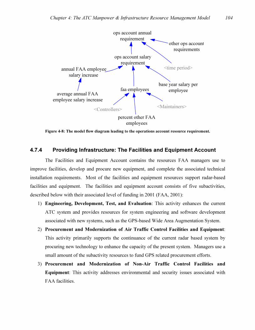
Chapter 4: The ATC Manpower & Infrastructure Resource Management Model 104
faa employees
percent other FAA
employees
annual FAA employee
salary increase
ops account salary
requirement
base year salary per
employeeaverage annual FAA
employee salary increase
<Controllers>
other ops account
requirements
ops account annual
requirement
<Maintainers>
<time period>
Figure 4-8: The model flow diagram leading to the operations account resource requirement.
4.7.4 Providing Infrastructure: The Facilities and Equipment Account
The Facilities and Equipment Account contains the resources FAA managers use to
improve facilities, develop and procure new equipment, and complete the associated technical
installation requirements. Most of the facilities and equipment resources support radar-based
facilities and equipment. The facilities and equipment account consists of five subactivities,
described below with their associated level of funding in 2001 (FAA, 2001):
1) Engineering, Development, Test, and Evaluation: This activity enhances the current
ATC system and provides resources for system engineering and software development
associated with new systems, such as the GPS-based Wide Area Augmentation System.
2) Procurement and Modernization of Air Traffic Control Facilities and Equipment:
This activity primarily supports the continuance of the current radar based system by
procuring new technology to enhance the capacity of the present system. Managers use a
small amount of the subactivity resources to fund GPS related procurement efforts.
3) Procurement and Modernization of Non-Air Traffic Control Facilities and
Equipment: This activity addresses environmental and security issues associated with
FAA facilities.

Chapter 4: The ATC Manpower & Infrastructure Resource Management Model 105
4) Facilities and Equipment Mission Support: This activity consists of systems
engineering, integration, and management of FAA capital improvement programs, such
as automation, communications, and surveillance.
5) Personnel and Related Expenses: This account pays for travel and other expenses
associated with FAA personnel who install equipment and implement procedures
initiated by managers of the facilities and equipment Account.
The model divides the resources in the facilities and equipment account into three
subcategories. The first category includes facilities occupied by people and the equipment used
in those facilities. The second category includes all the remaining equipment in the system that
supports radar-based ATC. The third category includes all equipment that supports GPS-based
ATC. It is not an FAA accounting practice to distribute the facilities and equipment budget
among the three categories. Therefore, Table 4-19 provides a breakdown of the distribution of
resources from the FAA that fit into the three categories. The three categories reside in the
model as an assumption of how the FAA distributes between radar-based or GPS-based ATC.
Table 4-19: The distribution of Facilities and Equipment resources among six categories.
Facilities & Equipment Programs
Category 2000 $M
2001 $M
2002 $M
Avg $M
Avg %
En Route Equipment Equipment 268 320 446 345 Terminal Equipment Equipment 112 117 105 111 Landing & Nav Aids GPS 114 112 66 97
Research, Test & Eval Facility 13 14 16 14 Advanced Technology GPS 43 91 63 66
En Route Facilities E Facility 301 385 478 388 Terminal Facilities T Facility 427 530 587 515
Flight Services Facilities F Facility 24 48 65 46 Landing & Nav Aids Eqpt Equipment 31 177 124 111
Other Facilities Facility 42 70 104 72 Support Eqpt Equipment 90 96 101 96
Support Eqpt for Facilities Facility 91 95 101 96 Training Facilities Facility 0 11 15 9
System Support for Eqpt Equipment 111 131 133 125 System Support for Facilities Facility 112 131 134 126
Personnel for Eqpt Equipment 148 161 183 164 Personnel for Facilities Facility 147 162 184 164
F & E TOTAL: 2,034 2,651 2,914 2,533 En Route FACILITY TOTAL: 301 385 478 388 15% Terminal FACILITY TOTAL: 427 530 587 515 20%
FSS FACILITY TOTAL: 24 45 65 45 2% Other FACILITY TOTAL: 405 481 554 480 19%
Radar EQUIPMENT TOTAL: 761 1,002 1,092 952 37% GPS TOTAL: 157 203 129 163 6%
(Source: FAA Budget in Brief, 2001 & 2002)

Chapter 4: The ATC Manpower & Infrastructure Resource Management Model 106
The model uses the Table 4-19 baseline distribution of resources within the facilities and
equipment account of 15% for en route facilities, 20% for terminal facilities, 2% for Flight
Service Stations, 19% for other facilities, 37% for radar-based equipment, and 6% for GPS-based
equipment. Annually, the Facilities and Equipment budget usually consumes approximately
23% of the entire FAA budget as indicated in Table 4-11. The six categories in Table 4-19
further refine the distribution of the facilities and equipment account. Within the model, each
facility and piece of equipment requires a portion of the facilities and equipment budget in order
to modernize and replace components of the ATC system. The $515M for Terminal facilities
represents 20% of the F&E account and further subdivides into $148M for TRACONs (6% of
F&E) and three types of control towers: $222M for AC towers (9%), $85M for AT towers (3%),
and $63M for GA towers (2%). Accordingly, Table 4-20 provides the assignment of the portion
of the facilities and equipment budget to each item listed in the first column.
Table 4-20: Facilities and equipment account requirements generated by the ATC infrastructure.
Facility or Equipment Number in ATC System in 1998
Total Required F&E Budget in 1998
Annual $M per in 1998
ARTCC 21 1900*0.15 = $285M 285/21 = 13.57 TRACON 170 1900* 0.06 = $114M 114/170 = 0.67
AC Towers 170 1900 * 0.09 = $171M 171/170 = 1.01 AT Towers 135 1900 * 0.03 = $57M 57/135 = 0.42 GA Towers 160 1900 * 0.02 = $38M 38/160 = 0.35
FSSs 137 1900 * 0.02 = $38M 38/137 = 0.28 Radar Equipment 7,468 1900 * 0.37 = $703M 703/7468 = 0.09
GPS Equipment 250 1900* 0.06 = $114M 114/250 = 0.46 Other Facilities 1 1900* 0.19 = $361M 361
Total: $1,900M
The first column of Table 4-20 lists the facilities or equipment that require funding from
the facilities and equipment account for modernization or replacement. The second column lists
the number of each type facility or equipment in the ATC system during the model base year
1998. The number of AC Towers, AT Towers, and GA Towers reflects the data in section 4.8.2.
The number of pieces of radar equipment comes from Table 4-26. The number of pieces of GPS
equipment comes from an estimate of installations discussed in section 4.9.2. The third column
adjusts the facilities and equipment budget numbers from Table 4-19 to revise them down to the
1998 levels by multiplying each entry by the ratio of the total facilities and equipment account in

Chapter 4: The ATC Manpower & Infrastructure Resource Management Model 107
1998 divided by the average total facilities and equipment account value in Table 4-19. The
final column provides the amount used in the model to determine the required facilities and
equipment account based on the numbers of facilities and equipment in the ATC system as it
dynamically changes over time.
Within the model, a combination of the budget distribution ratios above and the feedback
mechanisms caused by interactions of the subsystems influences the distribution of the resources
in the facilities and equipment account among the different areas: facilities, radar-based
equipment, and GPS-based equipment. The FAA policy regarding the distribution of resources
to support the radar-based approach to ATC or the GPS-based approach to ATC will further
refine the funding levels of facilities and equipment throughout the system.
Figure 4-9 shows the decision-making associated with the flow of resources through the
facilities and equipment account. The number of entities within the stocks in the system and the
costs per entity create an overall budget requirement for the Facilities and Equipment Account.
The model also includes a parameter accounting for 19% of the Facilities and Equipment
requirement as a system-wide overhead requirement. Finally, the model includes a parameter to
account for the historic growth rate within the Facilities and Equipment Account. The
“operating cost growth factor” stems from the linear increase of 3% annual growth from the
Facilities and Equipment account of $2,095M in 1991 to $2,914M in 2002.

Chapter 4: The ATC Manpower & Infrastructure Resource Management Model 108
<Centers>
<TRACONs> <AC Towers>
<FSSs>
<Radar based
Equipment>
<GPS based
Equipment>
center avg annual
cost
TRACON avg
annual cost
ac tower avg
annual cost
FSS avg annual
cost
radar eqpt avg
annual cost
GPS eqpt avg
annual cost
facilities and equipt
annual requirement
<AT Towers>
<GA Towers>
at tower avg
annual cost
ga tower avg
annual cost
gps eqpt annual
cost
fss annual cost
radar eqpt annual
cost
centers annual cost
tracon annual cost
ac towers annual
costat towers annual
cost
ga towers annual
cost
operating cost
growth factor
other facilities
costs
<time period>
f and e cost growth
multiplier
ramp increase in
01 and 02
ramp amount for F
and E
percent
growth
Figure 4-9: The requirement for resources to support the facilities and equipment account.
4.7.5 ATC Revenue: The Airport and Airway Trust Fund
Federal law allows tax receipts from sources such as passenger tickets, landing fees, and
aviation fuel sales to accumulate in an account that is the sole source of resources for the FAA’s
capital and operations accounts. Table 4-21 shows the distribution of these fund sources during
the past few years as well as estimates for the next two years. In 2001, the fund collected $10
billion in taxes, gained $0.88 billion in interest, and had an uncommitted balance of $7.5 billion
(FAA, 2001).
Table 4-21: Sources of revenue for the Airport and Airways Trust Fund.
Trust Fund Receipts from Excise Taxes
1998 1999 2000 2001 2002 (est)
2003 (est)
Passenger Ticket Tax $5,445 5,941 5,103 4,805 4,248 4,763 Passenger Flight Segment Tax 547 1,339 1,655 1,556 1,634 1,771 Waybill 313 412 500 493 585 606 Fuel Tax 659 1,009 887 769 849 882 Intl Departure/Arrival Tax 948 1,484 1,349 1,336 1,371 1,401 Rural Airports Tax 48 57 86 82 93 96 Frequent Flyer Tax 141 149 159 150 158 162 Interest on Investments 543 698 805 882 869 623 Offsetting Collections NR 32 144 76 224 136
Total 8,654 11,121 10,688 10,149 10,031 10,440
Source: FAA, 2002a
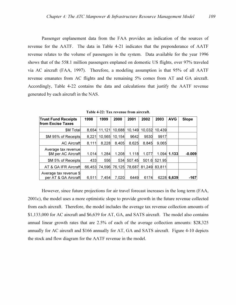
Chapter 4: The ATC Manpower & Infrastructure Resource Management Model 109
Passenger enplanement data from the FAA provides an indication of the sources of
revenue for the AATF. The data in Table 4-21 indicates that the preponderance of AATF
revenue relates to the volume of passengers in the system. Data available for the year 1996
shows that of the 558.1 million passengers enplaned on domestic US flights, over 97% traveled
via AC aircraft (FAA, 1997). Therefore, a modeling assumption is that 95% of all AATF
revenue emanates from AC flights and the remaining 5% comes from AT and GA aircraft.
Accordingly, Table 4-22 contains the data and calculations that justify the AATF revenue
generated by each aircraft in the NAS.
Table 4-22: Tax revenue from aircraft.
Trust Fund Receipts from Excise Taxes
1998 1999 2000 2001 2002 2003 AVG Slope
$M Total 8,654 11,121 10,688 10,149 10,032 10,439
$M 95% of Receipts 8,221 10,565 10,154 9642 9530 9917
AC Aircraft 8,111 8,228 8,405 8,625 8,845 9,065
Average tax revenue $M per AC Aircraft 1.014 1.284 1.208 1.118 1.077 1.094 1.133 -0.009
$M 5% of Receipts 433 556 534 507.45 501.6 521.95
AT & GA IFR Aircraft 66,453 74,596 76,125 78,687 81,249 83,811
Average tax revenue $ per AT & GA Aircraft 6,511 7,454 7,020 6449 6174 6228 6,639 -167
However, since future projections for air travel forecast increases in the long term (FAA,
2001c), the model uses a more optimistic slope to provide growth in the future revenue collected
from each aircraft. Therefore, the model includes the average tax revenue collection amounts of
$1,133,000 for AC aircraft and $6,639 for AT, GA, and SATS aircraft. The model also contains
annual linear growth rates that are 2.5% of each of the average collection amounts: $28,325
annually for AC aircraft and $166 annually for AT, GA and SATS aircraft. Figure 4-10 depicts
the stock and flow diagram for the AATF revenue in the model.

Chapter 4: The ATC Manpower & Infrastructure Resource Management Model 110
<AC Aircraft>
base year tax revenue
per AC aircraft
avg annual increase in
AC tax revenue
tax revenue from ACaircraft based on year
collected
tax revenue from
AC aircraft
avg annual increase in
GAAT tax revenue
tax revenue from GAATaircraft based on year
collected
base year tax revenue
per GAAT aircraft tax revenue from GA
AT and SATS acft
<GA
Aircraft><SATS Aircraft>
<AT Aircraft>
tax revenue adjustment
based on budget function
effect of budget
ratio
<time period>
effect of peopleshortage on tax
revenue
<controller
discrepancy>
<maintainer
discrepancy>
<budget ratio>
<feedback to AC
revenue>
<feedback to GA
AT>
Figure 4-10: The stock and flow diagram of the revenue collected by the AATF.
Table 4-23 below includes another important piece of the Budget Subsystem. The AATF
annually collects interest on invested assets. The average interest rate over the years 1998 to
2003 was 7.2%. The model includes a conservative interest rate of 6.5% of the AATF.
Table 4-23: The AATF gains approximately 7% interest annually.
Trust Fund 1998 1999 2000 2001 2002 (est)
2003 (est)
Total AATF 8,654 11,121 10,688 10,149 10,031 10,440Interest on Investments 543 698 805 882 869 623
Percent of AATF 6.3% 6.3% 7.5% 8.7% 8.7% 6.0%
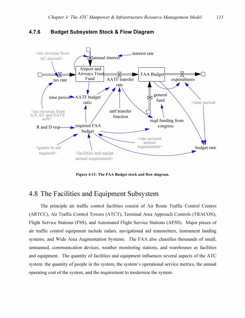
Chapter 4: The ATC Manpower & Infrastructure Resource Management Model 111
4.7.6 Budget Subsystem Stock & Flow Diagram
Airport andAirways Trust
Fund
<ops accountannual
requirement>
time period
<tax revenue from
AC aircraft>
<tax revenue fromGA AT and SATS
acft>
tax rate
<facilities and equipt
annual requirement>
<grants in aid
required>
FAA BudgetAATF transfer
rate
expenditures
general
fund
reqd funding from
congressR and D reqt required FAA
budget
annual interestinterest rate
budget ratio
AATF budget
ratio
aatf transfer
function
<time period>
Figure 4-11: The FAA Budget stock and flow diagram.
4.8 The Facilities and Equipment Subsystem
The principle air traffic control facilities consist of Air Route Traffic Control Centers
(ARTCC), Air Traffic Control Towers (ATCT), Terminal Area Approach Controls (TRACON),
Flight Service Stations (FSS), and Automated Flight Service Stations (AFSS). Major pieces of
air traffic control equipment include radars, navigational aid transmitters, instrument landing
systems, and Wide Area Augmentation Systems. The FAA also classifies thousands of small,
unmanned, communication devices, weather monitoring stations, and warehouses as facilities
and equipment. The quantity of facilities and equipment influences several aspects of the ATC
system: the quantity of people in the system, the system’s operational service metrics, the annual
operating cost of the system, and the requirement to modernize the system.

Chapter 4: The ATC Manpower & Infrastructure Resource Management Model 112
Although ATC facilities are the heart of the current ATC system, theoretically, they will
not be an essential part of SATS. The equipment that supports GPS navigation and aircraft “self-
separation” will provide the greatest support to SATS. Navigation equipment generally supports
either the current radar-based ATC system or the evolving GPS-based ATC system required by
SATS aircraft. The principle facilities in the modern ATC system consist of 21 centers, 470
control towers, 170 TRACONs, and 137 flight service stations.
4.8.1 Centers, Approach Controls, and Flight Service Stations
The FAA has the authority to separate civilian and military air traffic in controlled
airspace in the US. Currently, the FAA subdivides its authority among 21 air route traffic
control centers (ARTCC), down from 24 centers in the 1980s. Normally, the ARTCC separates
en route traffic and delegates the separation of traffic near airports to the FAA or military ATC
facility at the airport (Nolan, 1999). A modeling assumption is that there will be no further
growth in the number of centers. Rather, efficiencies from automation will cause the number of
centers to decline by two centers consolidating every 7 years. The expansion of free flight may
change the nature of the center controllers’ duties from air traffic control to air traffic
management and monitoring.
Approach controllers monitor radar displays to separate aircraft within a distance of
approximately 20 miles from an airport to facilitate the transition of arriving or departing
aircraft. Approach controllers ease the workload on both tower controllers and controllers in the
air traffic control centers (Nolan, 1999). There are currently 170 Terminal Area Approach
Control (TRACON) facilities in the US ATC system. The model includes consolidation events
due to technological efficiencies among TRACONs at the rate of one consolidation every 10
years.
Controllers at Flight Service Stations (FSS) and Automated Flight Service Stations
(AFSS) provide air traffic control services consisting of weather briefings, flight advisories,
radio communications, flight planning, and search and rescue coordination (Lammes, 2002). In
the model, FSSs and AFSSs perform the same functions and reside in the stock labeled FSS.
The model uses a 1998 base year value of 137 FSSs with a growth rate of one new FSS annually.
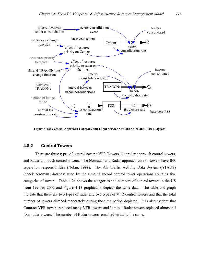
Chapter 4: The ATC Manpower & Infrastructure Resource Management Model 113
Centerscenter
consolidation rate
center consolidation
event
interval between
center consolidationscenters
consolidated
TRACONs
tracon
consolidation rate
tracons
consolidatedtracon
consolidation event
interval between
tracon consolidations
FSSs
fss construction
rate
fss closure rate
fss and TRACON rate
change function
<resource priority
to radar> effect of resource
priority to radar on
facilities
normal fss
construction rate
base year centers
base year
TRACONs
center rate change
functioneffect of resource
priority on Centers
base year FSS
<effect of budget
ratio>
Figure 4-12: Centers, Approach Controls, and Flight Service Stations Stock and Flow Diagram
4.8.2 Control Towers
There are three types of control towers: VFR Towers, Nonradar-approach control towers,
and Radar-approach control towers. The Nonradar and Radar-approach control towers have IFR
separation responsibilities (Nolan, 1999). The Air Traffic Activity Data System (ATADS)
(check acronym) database used by the FAA to record control tower operations contains five
categories of towers. Table 4-24 shows the categories and numbers of control towers in the US
from 1990 to 2002 and Figure 4-13 graphically depicts the same data. The table and graph
indicate that there are two types of radar and two types of VFR control towers and that the total
number of towers climbed moderately during the time period depicted. It is also evident that
Contract VFR towers replaced many VFR towers and Limited Radar towers replaced almost all
Non-radar towers. The number of Radar towers remained virtually the same.
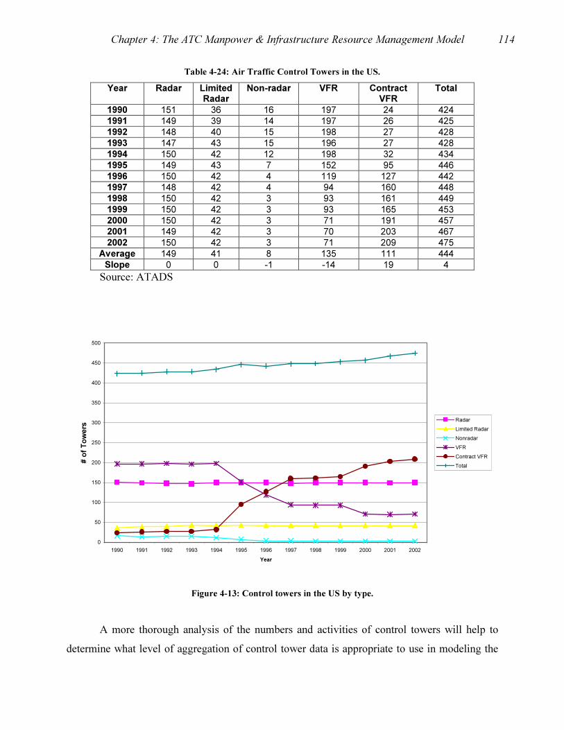
Chapter 4: The ATC Manpower & Infrastructure Resource Management Model 114
Table 4-24: Air Traffic Control Towers in the US.
Year Radar Limited Radar
Non-radar VFR Contract VFR
Total
1990 151 36 16 197 24 424 1991 149 39 14 197 26 425 1992 148 40 15 198 27 428 1993 147 43 15 196 27 428 1994 150 42 12 198 32 434 1995 149 43 7 152 95 446 1996 150 42 4 119 127 442 1997 148 42 4 94 160 448 1998 150 42 3 93 161 449 1999 150 42 3 93 165 453 2000 150 42 3 71 191 457 2001 149 42 3 70 203 467 2002 150 42 3 71 209 475
Average 149 41 8 135 111 444 Slope 0 0 -1 -14 19 4
Source: ATADS
0
50
100
150
200
250
300
350
400
450
500
1990 1991 1992 1993 1994 1995 1996 1997 1998 1999 2000 2001 2002
Year
# o
f T
ow
ers
Radar
Limited Radar
Nonradar
VFR
Contract VFR
Total
Figure 4-13: Control towers in the US by type.
A more thorough analysis of the numbers and activities of control towers will help to
determine what level of aggregation of control tower data is appropriate to use in modeling the

Chapter 4: The ATC Manpower & Infrastructure Resource Management Model 115
facilities in the ATC system. Figure 4-14 depicts the average annual number of total instrument
operations for all control towers in the US. Four towers, Chicago, Dallas-Fort Worth, Atlanta,
and Los Angeles, each had over 700,000 annual operations. The other 470 control towers had
annual operations counts ranging from over 500,000 to almost zero.
Average Annual Total Operations per Tower
0
100000
200000
300000
400000
500000
600000
700000
800000
900000
1000000
0 100 200 300 400 500 600
Towers
Op
era
tio
ns
Figure 4-14: Average annual total Operations for all control towers
Table 4-25 contains the average number of operations for each of the five categories of
control towers. Figure 4-15 depicts the same data. The data indicate that Limited Radar towers
conduct about 45% of all operations. Radar towers continue to operate at a relatively steady rate.
The VFR towers are experiencing the greatest growth in operations. Contract VFR towers are
increasing operations at a modest rate and Nonradar towers are decreasing operations. It appears
that the VFR towers manned by FAA air traffic controllers are the VFR towers with the highest
rate of operations and the VFR towers that become Contract VFR towers are those with the
lower operational rates among all VFR towers. Further analysis of the control tower data at the
group and individual tower level of analysis will determine the homogeneity of the towers.

Chapter 4: The ATC Manpower & Infrastructure Resource Management Model 116
Table 4-25: Average annual operations per type of control tower.
Year Radar Limited Radar
Nonradar VFR Contract VFR
1990 133,387 318,095 60,478 124,809 54,4401991 140,395 322,954 69,011 137,006 60,0171992 140,229 326,081 70,599 134,341 61,7381993 139,900 313,958 70,276 127,314 61,0371994 138,508 339,466 78,905 122,728 58,8871995 138,221 334,970 94,462 146,701 46,8061996 135,363 344,583 58,606 162,946 59,0481997 140,050 347,396 55,724 188,327 65,0831998 141,581 349,204 67,147 181,311 76,2161999 148,828 360,232 43,909 187,584 79,2352000 149,937 362,616 41,455 215,888 81,2202001 144,459 353,125 37,900 200,266 76,137
Average 140,905 339,390 62,373 160,768 64,989Slope 972 4,164 -2,812 8,377 2,303
Average Ops per Type of Control Tower
0
50,000
100,000
150,000
200,000
250,000
300,000
350,000
400,000
1988 1990 1992 1994 1996 1998 2000 2002
Year
Av
era
ge
Op
s
Radar
Limited Radar
Nonradar
VFR
Contract VFR
Figure 4-15: Average annual operations per type of control tower.
The ATADS data displayed in the tables and graphs above reflect the operations of all
domestic air carrier, general aviation, air taxi, and military aircraft. The tables and graphs below
provide group and individual level insight to determine the best method to incorporate control

Chapter 4: The ATC Manpower & Infrastructure Resource Management Model 117
towers into the model. The information presented below leads to the homogeneous grouping of
control towers into thee core groups as the appropriate level of analysis for the modeling effort.
Figure 4-16 contains data for the average AC operations per tower from 1990 to 2001.
The data shows that 99% of the AC activity occurred at the top 170 towers. Therefore, the
model includes all the top 170 towers in the core part of the ATC system that supports AC
operations, regardless of the presence of SATS aircraft. The data indicates that AC operations
occurred at 111 out of 150 Radar towers and 39 of 42 Limited Radar air traffic control towers.
Some limited Radar and Radar towers had minimal AC operations as they primarily serve GA
and Air Taxi operations in the vicinity of major AC airports.
Average AC Ops per Tower 1990-2001
0
100000
200000
300000
400000
500000
600000
700000
800000
0 100 200 300 400 500 600
Towers
Op
era
tio
ns
Avg
Figure 4-16: Average annual air carrier operations per tower.
Figure 4-17 shows the distribution of average Air Taxi (AT) operations per tower from
1990 to 2001. The data shows that the bulk of Air Taxi aircraft operations occurred at the top
300 towers. All of the 170 towers supporting the top AC operations are also in the top 300
towers that support AT operations. All 42 limited-radar towers are within the top 300 towers.
Of the 150 radar towers, 145 are within the top 300 towers. Many of the control towers that
served Air Taxi aircraft changed from VFR towers to Contract VFR towers.

Chapter 4: The ATC Manpower & Infrastructure Resource Management Model 118
Average Air Taxi Ops per Tower
0
50000
100000
150000
200000
250000
0 100 200 300 400 500 600
Tower
Op
era
tio
ns
AVG
Figure 4-17: Average annual air taxi operations per tower.
Figure 4-18 indicates that GA operations occur throughout most airports with control
towers in the NAS. In fact, 460 control towers provide at least 8,000 annual control tower
operations for GA aircraft. Of the 460, approximately 150 provide almost all their services to
GA aircraft, with little to none of the services going to AC or AT aircraft. These 150 towers
serve the core GA-only ATC requirements. There are only about ten towers that provide less
than 8,000 total operations for all types of aircraft combined. These ten represent only 2% of all
control towers, indicating that the system does not contain many underutilized assets.
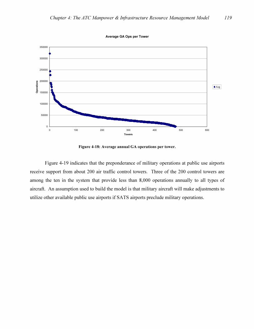
Chapter 4: The ATC Manpower & Infrastructure Resource Management Model 119
Average GA Ops per Tower
0
50000
100000
150000
200000
250000
300000
350000
0 100 200 300 400 500 600
Towers
Op
era
tio
ns
Avg
Figure 4-18: Average annual GA operations per tower.
Figure 4-19 indicates that the preponderance of military operations at public use airports
receive support from about 200 air traffic control towers. Three of the 200 control towers are
among the ten in the system that provide less than 8,000 operations annually to all types of
aircraft. An assumption used to build the model is that military aircraft will make adjustments to
utilize other available public use airports if SATS airports preclude military operations.
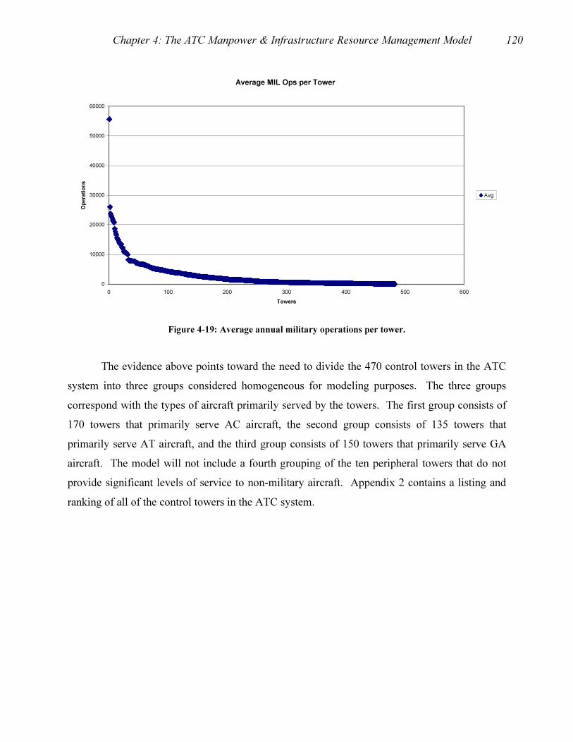
Chapter 4: The ATC Manpower & Infrastructure Resource Management Model 120
Average MIL Ops per Tower
0
10000
20000
30000
40000
50000
60000
0 100 200 300 400 500 600
Towers
Op
era
tio
ns
Avg
Figure 4-19: Average annual military operations per tower.
The evidence above points toward the need to divide the 470 control towers in the ATC
system into three groups considered homogeneous for modeling purposes. The three groups
correspond with the types of aircraft primarily served by the towers. The first group consists of
170 towers that primarily serve AC aircraft, the second group consists of 135 towers that
primarily serve AT aircraft, and the third group consists of 150 towers that primarily serve GA
aircraft. The model will not include a fourth grouping of the ten peripheral towers that do not
provide significant levels of service to non-military aircraft. Appendix 2 contains a listing and
ranking of all of the control towers in the ATC system.
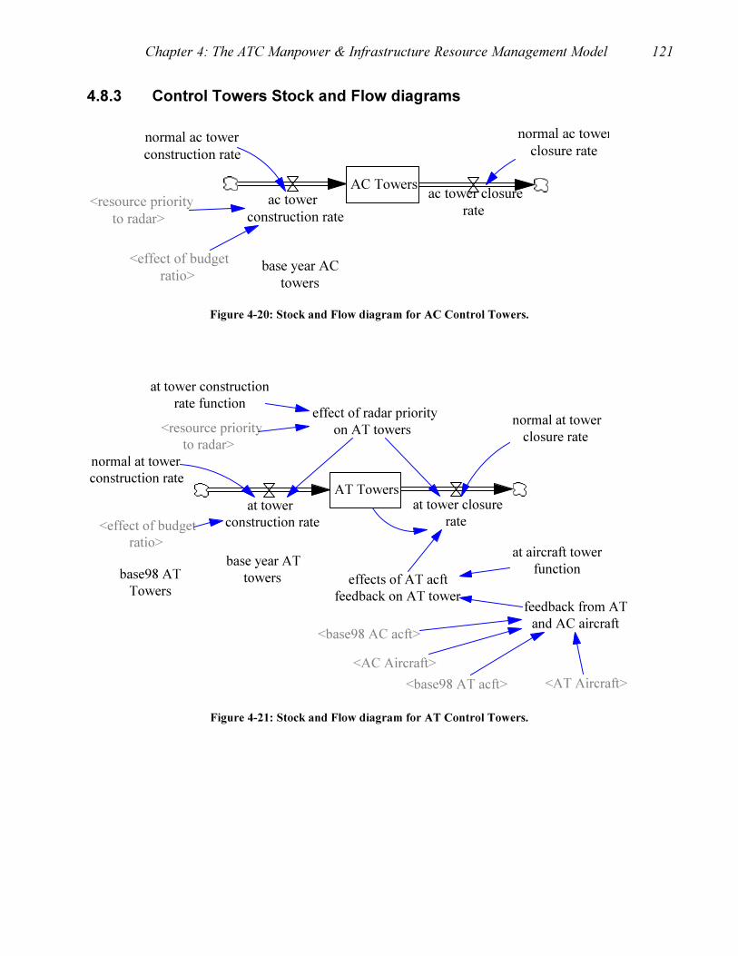
Chapter 4: The ATC Manpower & Infrastructure Resource Management Model 121
4.8.3 Control Towers Stock and Flow diagrams
AC Towersac tower
construction rate
ac tower closure
rate
normal ac tower
construction rate
normal ac tower
closure rate
<resource priority
to radar>
base year AC
towers
<effect of budget
ratio>
Figure 4-20: Stock and Flow diagram for AC Control Towers.
AT Towersat tower
construction rate
at tower closure
rate
normal at tower
construction rate
normal at tower
closure rate
at tower construction
rate function
<resource priority
to radar>
effect of radar priority
on AT towers
base year AT
towers
feedback from AT
and AC aircraft
at aircraft tower
functioneffects of AT acft
feedback on AT tower
<AT Aircraft>
<effect of budget
ratio>
base98 AT
Towers
<base98 AT acft>
<base98 AC acft>
<AC Aircraft>
Figure 4-21: Stock and Flow diagram for AT Control Towers.
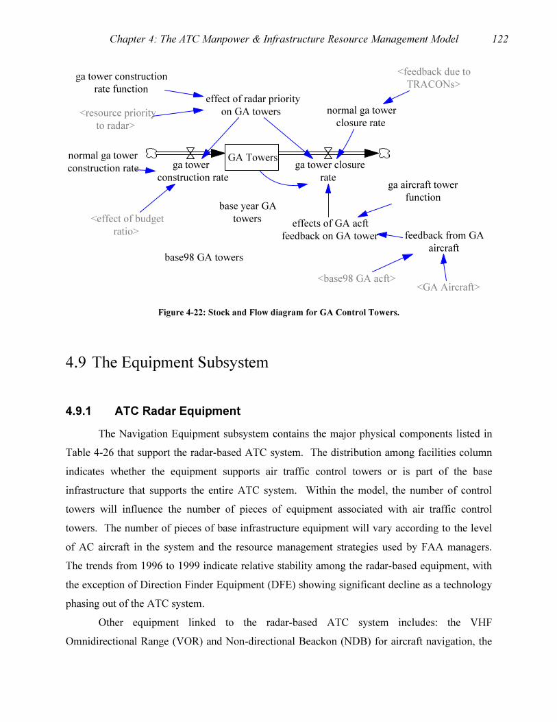
Chapter 4: The ATC Manpower & Infrastructure Resource Management Model 122
GA Towersga tower
construction rate
ga tower closure
rate
normal ga tower
construction rate
normal ga tower
closure rate
ga tower construction
rate function
<resource priority
to radar>
effect of radar priority
on GA towers
base year GA
towers
feedback from GA
aircraft
<GA Aircraft>
ga aircraft tower
function
effects of GA acft
feedback on GA tower
<feedback due to
TRACONs>
<effect of budget
ratio>
base98 GA towers
<base98 GA acft>
Figure 4-22: Stock and Flow diagram for GA Control Towers.
4.9 The Equipment Subsystem
4.9.1 ATC Radar Equipment
The Navigation Equipment subsystem contains the major physical components listed in
Table 4-26 that support the radar-based ATC system. The distribution among facilities column
indicates whether the equipment supports air traffic control towers or is part of the base
infrastructure that supports the entire ATC system. Within the model, the number of control
towers will influence the number of pieces of equipment associated with air traffic control
towers. The number of pieces of base infrastructure equipment will vary according to the level
of AC aircraft in the system and the resource management strategies used by FAA managers.
The trends from 1996 to 1999 indicate relative stability among the radar-based equipment, with
the exception of Direction Finder Equipment (DFE) showing significant decline as a technology
phasing out of the ATC system.
Other equipment linked to the radar-based ATC system includes: the VHF
Omnidirectional Range (VOR) and Non-directional Beackon (NDB) for aircraft navigation, the
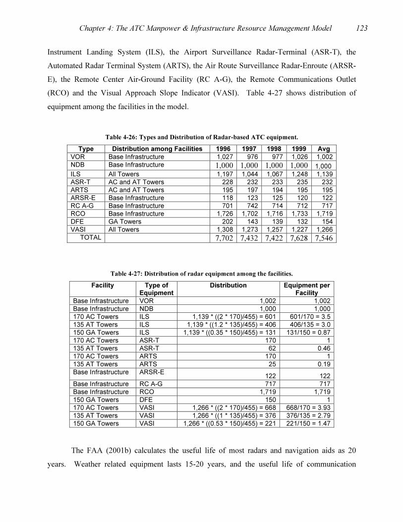
Chapter 4: The ATC Manpower & Infrastructure Resource Management Model 123
Instrument Landing System (ILS), the Airport Surveillance Radar-Terminal (ASR-T), the
Automated Radar Terminal System (ARTS), the Air Route Surveillance Radar-Enroute (ARSR-
E), the Remote Center Air-Ground Facility (RC A-G), the Remote Communications Outlet
(RCO) and the Visual Approach Slope Indicator (VASI). Table 4-27 shows distribution of
equipment among the facilities in the model.
Table 4-26: Types and Distribution of Radar-based ATC equipment.
Type Distribution among Facilities 1996 1997 1998 1999 Avg VOR Base Infrastructure 1,027 976 977 1,026 1,002 NDB Base Infrastructure 1,000 1,000 1,000 1,000 1,000 ILS All Towers 1,197 1,044 1,067 1,248 1,139 ASR-T AC and AT Towers 228 232 233 235 232 ARTS AC and AT Towers 195 197 194 195 195 ARSR-E Base Infrastructure 118 123 125 120 122 RC A-G Base Infrastructure 701 742 714 712 717 RCO Base Infrastructure 1,726 1,702 1,716 1,733 1,719 DFE GA Towers 202 143 139 132 154 VASI All Towers 1,308 1,273 1,257 1,227 1,266
TOTAL 7,702 7,432 7,422 7,628 7,546
Table 4-27: Distribution of radar equipment among the facilities.
Facility Type of Equipment
Distribution Equipment per Facility
Base Infrastructure VOR 1,002 1,002 Base Infrastructure NDB 1,000 1,000 170 AC Towers ILS 1,139 * ((2 * 170)/455) = 601 601/170 = 3.5 135 AT Towers ILS 1,139 * ((1.2 * 135)/455) = 406 406/135 = 3.0 150 GA Towers ILS 1,139 * ((0.35 * 150)/455) = 131 131/150 = 0.87 170 AC Towers ASR-T 170 1 135 AT Towers ASR-T 62 0.46 170 AC Towers ARTS 170 1 135 AT Towers ARTS 25 0.19 Base Infrastructure ARSR-E
122 122 Base Infrastructure RC A-G 717 717 Base Infrastructure RCO 1,719 1,719 150 GA Towers DFE 150 1 170 AC Towers VASI 1,266 * ((2 * 170)/455) = 668 668/170 = 3.93 135 AT Towers VASI 1,266 * ((1 * 135)/455) = 376 376/135 = 2.79 150 GA Towers VASI 1,266 * ((0.53 * 150)/455) = 221 221/150 = 1.47
The FAA (2001b) calculates the useful life of most radars and navigation aids as 20
years. Weather related equipment lasts 15-20 years, and the useful life of communication
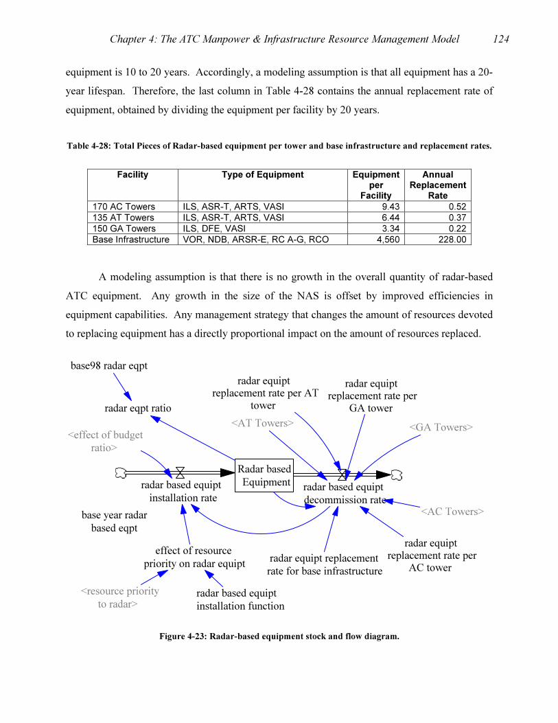
Chapter 4: The ATC Manpower & Infrastructure Resource Management Model 124
equipment is 10 to 20 years. Accordingly, a modeling assumption is that all equipment has a 20-
year lifespan. Therefore, the last column in Table 4-28 contains the annual replacement rate of
equipment, obtained by dividing the equipment per facility by 20 years.
Table 4-28: Total Pieces of Radar-based equipment per tower and base infrastructure and replacement rates.
Facility Type of Equipment Equipment
per Facility
Annual Replacement
Rate 170 AC Towers ILS, ASR-T, ARTS, VASI 9.43 0.52135 AT Towers ILS, ASR-T, ARTS, VASI 6.44 0.37150 GA Towers ILS, DFE, VASI 3.34 0.22Base Infrastructure VOR, NDB, ARSR-E, RC A-G, RCO 4,560 228.00
A modeling assumption is that there is no growth in the overall quantity of radar-based
ATC equipment. Any growth in the size of the NAS is offset by improved efficiencies in
equipment capabilities. Any management strategy that changes the amount of resources devoted
to replacing equipment has a directly proportional impact on the amount of resources replaced.
Radar based
Equipmentradar based equipt
installation rateradar based equipt
decommission rate
radar equiptreplacement rate per
AC tower
<AC Towers>
radar equiptreplacement rate per AT
tower
<AT Towers>
radar equiptreplacement rate per
GA tower
<GA Towers>
radar equipt replacement
rate for base infrastructure
radar based equipt
installation function
effect of resource
priority on radar equipt
<resource priority
to radar>
base year radar
based eqpt
<effect of budget
ratio>
base98 radar eqpt
radar eqpt ratio
Figure 4-23: Radar-based equipment stock and flow diagram.
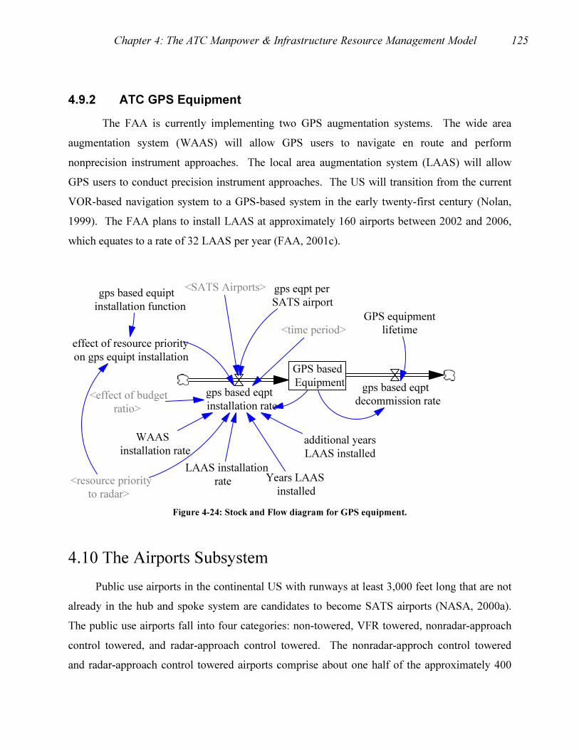
Chapter 4: The ATC Manpower & Infrastructure Resource Management Model 125
4.9.2 ATC GPS Equipment
The FAA is currently implementing two GPS augmentation systems. The wide area
augmentation system (WAAS) will allow GPS users to navigate en route and perform
nonprecision instrument approaches. The local area augmentation system (LAAS) will allow
GPS users to conduct precision instrument approaches. The US will transition from the current
VOR-based navigation system to a GPS-based system in the early twenty-first century (Nolan,
1999). The FAA plans to install LAAS at approximately 160 airports between 2002 and 2006,
which equates to a rate of 32 LAAS per year (FAA, 2001c).
GPS based
Equipmentgps based eqpt
installation rate
gps based eqpt
decommission rate
GPS equipment
lifetime
WAAS
installation rate
LAAS installation
rate Years LAAS
installed
gps based equipt
installation function
<resource priority
to radar>
effect of resource priority
on gps equipt installation
additional years
LAAS installed
gps eqpt per
SATS airport
<SATS Airports>
<time period>
<effect of budget
ratio>
Figure 4-24: Stock and Flow diagram for GPS equipment.
4.10 The Airports Subsystem
Public use airports in the continental US with runways at least 3,000 feet long that are not
already in the hub and spoke system are candidates to become SATS airports (NASA, 2000a).
The public use airports fall into four categories: non-towered, VFR towered, nonradar-approach
control towered, and radar-approach control towered. The nonradar-approch control towered
and radar-approach control towered airports comprise about one half of the approximately 400

Chapter 4: The ATC Manpower & Infrastructure Resource Management Model 126
airports in the hub and spoke system. A modeling assumption is that the towered airports in the
hub and spoke system will continue to remain and operate according to historical growth rates.
The existing non-towered airports, possibly some of the VFR towered airports, and VFR towered
reliever airports are candidates to become SATS airports. These airports reside within two
stocks in the model: the nonSATS airports stock and the SATS airports stock depicted in Figure
4-25 below.
Advocates for SATS claim that all of the approximately 5,400 public use airports in the US
are potential SATS airports. However, the model uses a pool of potential airports that is
significantly smaller than the pool advocated by NASA. Of the 5,400 public use airports, only
3,344 are eligible to receive Grants-in-Aid funding for airport improvement (Department of
Transportation, 1999). Of the 3,344 eligible for funding, 419 are primary airports that support
the commercial airline system and 125 are non-primary commercial that support cargo
operations. Both types of commercial airports would not be available as SATS only airports.
Therefore, the model uses 334 reliever airports and 2,472 GA airports for a total of 2,806
potential SATS airports. In the model, an airport from the pool of 2,806 becomes a SATS airport
when there is sufficient funding available for conversion and the conversion is in keeping with
the resource management priority to expand the GPS-based ATC system.
Many public use airports require significant improvements, such as runway improvements
and lighting, as indicated below in Table 4-29. However, as indicated in the earlier description
of the Budget Subsystem and as depicted in Table 4-12 above, the pool of 2,806 potential SATS
airports usually receive at best 18% of the entire Grants-in-Aid funding. Most of the Grants-in-
Aid funding supports the hub and spoke system.
Table 4-29: Many Public Use Airports require improvements.
Type 1980 1985 1990 1991 1992 1993 1994 1995 1996 1997 1998 1999 Public Use 4,814 5,858 5,589 5,551 5,545 5,538 5,474 5,415 5,389 5,357 5,352 5,354 # Unlighted 1,627 1,869 1,598 1,560 1,536 1,506 1,451 1,392 1,374 1,361 1,349 1,274 # Unpaved 1,333 1,951 1,638 1,582 1,575 1,540 1,483 1,446 1,417 1,393 1,381 1,381
According to the Aircraft Owners and Pilots Assn (AOPA), public use airports close at
the rate of one every two weeks (Aviation Week, 15 April 2002). The model uses only half that
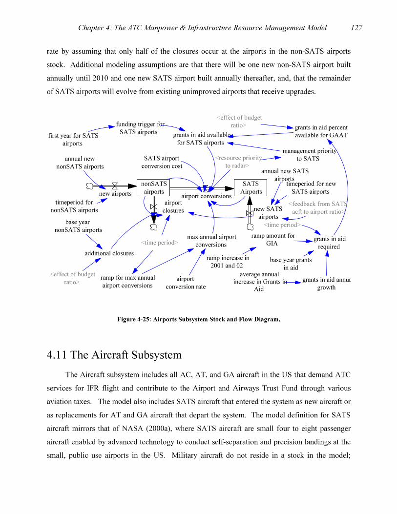
Chapter 4: The ATC Manpower & Infrastructure Resource Management Model 127
rate by assuming that only half of the closures occur at the airports in the non-SATS airports
stock. Additional modeling assumptions are that there will be one new non-SATS airport built
annually until 2010 and one new SATS airport built annually thereafter, and, that the remainder
of SATS airports will evolve from existing unimproved airports that receive upgrades.
SATS airport
conversion cost
SATS
Airports
nonSATS
airportsairport conversionsnew airports
grants in aid
required
base year grants
in aid
grants in aid annua
growth
grants in aid percent
available for GAATgrants in aid available
for SATS airports
management priority
to SATS
<time period>
average annualincrease in Grants in
Aid
first year for SATS
airports
funding trigger for
SATS airports
airport
closures
annual new
nonSATS airports
timeperiod for
nonSATS airports new SATS
airports
annual new SATS
airportstimeperiod for new
SATS airports
<resource priority
to radar>
base year
nonSATS airportsmax annual airport
conversions
ramp for max annual
airport conversionsairport
conversion rate
ramp increase in
2001 and 02
ramp amount for
GIA
additional closures
<time period>
<effect of budget
ratio>
<effect of budget
ratio>
<feedback from SATS
acft to airport ratio>
Figure 4-25: Airports Subsystem Stock and Flow Diagram,
4.11 The Aircraft Subsystem
The Aircraft subsystem includes all AC, AT, and GA aircraft in the US that demand ATC
services for IFR flight and contribute to the Airport and Airways Trust Fund through various
aviation taxes. The model also includes SATS aircraft that entered the system as new aircraft or
as replacements for AT and GA aircraft that depart the system. The model definition for SATS
aircraft mirrors that of NASA (2000a), where SATS aircraft are small four to eight passenger
aircraft enabled by advanced technology to conduct self-separation and precision landings at the
small, public use airports in the US. Military aircraft do not reside in a stock in the model;

Chapter 4: The ATC Manpower & Infrastructure Resource Management Model 128
however, variables representing relative ratios of military aircraft operations influence the
behavior of the modeled system.
Table 4-30 shows the number of AC, AT, and GA aircraft registered in the US from 1960
through the late 1990s. The figure shows that GA aircraft peaked in 1980, declined about 17%
through the mid 1990s and returned to the 1980 level by the end of the 1990s. The historic GA
aircraft growth rate is 2,489 yearly from 1990-2000. Therefore, the model includes a growth rate
of 2489/204710 = 0.01. Although the AT data is limited, the model uses a growth rate of 7%. In
the model, both the GA and AT growth rates adjust downward as SATS aircraft become more
popular. The historic AC aircraft growth rate is 177 yearly from 1960-1998. Therefore, the
model includes the assumption that there are 200 new aircraft registered and 23 aircraft
decommissioned or destroyed annually. The last two columns of the table provide additional
evidence of historic aircraft sales that correspond with growth rates.
Table 4-30: Aircraft registered in the US and new aircraft sales.
Year AC AT IFR GA All GA New AC New GA 1960 2,135 76,549 7,588 245
1965 2,125 95,442 11,852 233 1970 2,679 46,432 131,743 7,283 311 1975 2,495 168,475 14,072 315 1980 3,808 81,102 211,045 11,881 387 1985 4,678 69,590 210,654 2,029 278 1990 6,083 5,800 196,800 1,144 521 1991 6,054 199,600 1,021 589 1992 7,320 187,000 899 567 1993 7,297 180,700 964 408 1994 7,370 3,800 56,694 176,600 928 309 1995 7,411 4,100 56,895 188,100 1,077 256 1996 7,478 3,900 61,896 191,100 1,130 269 1997 7,616 4,948 192,400 1,569 374 1998 8,111 5,190 66,453 204,710 2,213 559 Slope 220 363 2,562 427
Growth 0.03 0.07 0.038 0.002
Source: 1960-1998 BTS
Table 4-31 shows the functional distribution among several categories of use of GA
aircraft over a 30-year time period. The trends in the distribution are consistent throughout all of
the functional subcategories of GA aircraft, with the exception that there has been a decline in

Chapter 4: The ATC Manpower & Infrastructure Resource Management Model 129
the percent of GA business aircraft. The data in Table 4-32 indicates that over 60% of GA
aircraft serve as personal means of transportation. Although some of the personal aircraft may
be SATS aircraft, a modeling assumption is that most SATS aircraft will serve as corporate,
business, or air taxi aircraft. Thus, the data in the two tables indicates that approximately 40% of
all GA aircraft would have a high propensity to become SATS aircraft. However, the model uses
a conservative estimate of conversions to SATS aircraft beginning at 0.5% in 2008 and rising to
5% by 2028.
Table 4-31: GA Aircraft by function.
GA Aircraft 1970 1980 1990 1994 1995 1996 1998 2000 Corporate 6,835 14,869 10,100 9,400 9,800 9,300 11,250 11,000 Business 26,900 49,391 33,100 26,500 26,200 28,200 32,611 25,200 Instructional 10,727 14,862 18,600 15,000 14,800 14,300 11,375 14,900 Personal 65,398 96,222 112,600 102,500 109,300 109,600 124,347 148,200 Air Taxi N
2 N 5,800 3,800 4,100 3,900 5,190 4,000
Government N N N N N 4,200 4,029 4,100 Other
1 19,913 33,721 14,610 13,206 21,905 19,604 13,910 8,100
TOTAL 131,743 211,045 196,800 172,400 188,100 191,100 204,710 217,500 % IFR
3 35% 38% 35% 33% 30% 32% 32% 28%
Source: NTS website and FAA Fact Book, February 2002.
1Other includes aerial application, aerial observation, sight seeing, and external load
2N = Data does not exist
3%IFR includes all categories except Personal and Other.
Table 4-32: Percent distribution of GA Aircraft by function.
GA Aircraft 1970 1980 1990 1994 1995 1996 1998 2000 Corporate 5% 7% 5% 5% 5% 5% 5% 5% Business 20% 23% 17% 15% 14% 15% 16% 12% Instructional 8% 7% 9% 9% 8% 7% 6% 7% Personal 50% 46% 57% 59% 58% 57% 61% 68% Air Taxi 0% 0% 3% 2% 2% 2% 3% 2% Government 0% 0% 0% 0% 0% 2% 2% 2% Other 15% 16% 7% 8% 12% 10% 7% 4%

Chapter 4: The ATC Manpower & Infrastructure Resource Management Model 130
AC Aircraftac aircraft
registration rate
ac aircraft
decommission rate
feedback due to
AC towers
<base year AC
towers>
<AC Towers>
normal AC acft
registration rate
feedback due to
Centers
<Centers><base year
centers>
feedback due to
TRACONs<base year
TRACONs>
<TRACONs>
ac acft
operational life
<time period>
base year AC acft
max ac acft system
capacity
<feedback AC
tower ratio>
<feedback AC
Center ratio>
<feedback AC
TRACON ratio>
<feedback AC AT
Tower ratio>
<feedback due to
radar eqpt>
Idle AC Acft
enter idlerate
depart idle rate
infrastructure
shortfallinfrastructure
shortfall function
effect ofinfrastructure
shortfall
AC aircraft registration
rate adjustment function
effect of idle acft
effect2 of
infrastructure shortfall
infrastructure
shortfall 2 func
Figure 4-26: AC Aircraft stock and flow diagram.
GA Aircraft
ga acft
registration rate
ga acft
decommission rate
SATS
AircraftSATS acft
registration rate
SATS acft
decommission rate
SATS acft
operational life
ga acft
operational life ga to SATS
conversion rate
new SATS acft
normal GA
growth rate
<time period>
AT Aircraftat acft
registration rateat acft
decommission rate
normal AT
growth rateat acft
operational life
at to SATS
conversion rate
feedback due to
AT towers
<AT Towers><feedback due to
Centers>
<feedback due to
TRACONs>
feedback due to
GA towers
<GA Towers>
base year GA
aircraft
base year AT acft
<airport
ratio>
<resource priority
to radar>
<feedback from SATS
acft to airport ratio>
<funding trigger for
SATS airports>
max GA acft
max AT acft
<impact of nonSATS
apts ratio>
<base98 AT
Towers>
<base98
GA towers>
base98 AT acft
base98 GA acft
<impact of nonSATS
apts ratio>
<feedback due to
radar eqpt>
<feedback due to
radar eqpt>
<SATS
experimental fleet>
Figure 4-27: AT, GA, and SATS aircraft stock and flow diagram.

Chapter 4: The ATC Manpower & Infrastructure Resource Management Model 131
Several factors influence the conversion rates to SATS aircraft in Figure 4-27. First, the
stocks of AT or GA aircraft provide the pools of potential SATS aircraft. Second, the SATS to
non-SATS airport ratio adjusts the flow of conversions. Third, the resource management
strategy, represented by the “resource priority to radar” auxiliary variable, changes the amount of
conversions. Finally, the level of funding available for SATS airports further adjusts the
conversion rate. These factors continually interact over time to create the dynamic behavior in
the model.
4.12 Summary
The model developed and presented above depicts the structure and relationships among the
key components of the ATC system that have bearing on the research questions. The modeling
process began with a system framework in the form of an influence diagram. The process then
involved identification of the exogenous and endogenous parts of the system. Finally, the
process led to the development of detailed submodels in the areas of people, budget, facilities
and equipment, airports, and aircraft. The next chapter will continue the System Dynamics
modeling process with the application of several procedures to verify and validate the model
developed above.

132
The utility of the model developed in Chapter 4 depends on its ability to provide accurate
and realistic results. The System Dynamics Modeling process requires verification and
validation of models to ensure they will be useful. The Vensim software includes several
functions that help modelers to verify and validate the results produced by models. The software
includes tools to ensure unit integrity, tools to trace numerical output, tools to observe graphical
output, tools to evaluate time steps, and tools to conduct sensitivity analysis. This chapter uses
many of the built in software tools in concert with several other tests and checks to create a
useful model. The other methods of validation include model simplicity tests, model parameter
checks, behavior reproduction tests, and behavior anomaly tests.
5.1 Verification
Model verification consists of several procedures to ensure that a model operates correctly
and as intended by the model developer. The System Dynamics model of ATC resource
management strategies operates in the Vensim language. Vensim has embedded tools to aid in
model verification. Modelers can also verify the accuracy of their works by running them on
other computers to verify that the software creates the same output. Finally, another useful
verification technique is to trace numerical values through the system.
5.1.1 Use Vensim Verification Tools
The Vensim software includes the capability to automatically verify the mathematical
structure of equations input through the Vensim equation editor. The software checks the syntax
of the equation and identifies errors such as an imbalance of parentheses. The software also
identifies missing or improper variables in the equation. The equation editor is intuitively sound
as a graphic user interface to align the mathematical equations in the model with the graphic
structure of the model’s stock and flow diagrams.
In addition to the syntax checks made in the equation editor, the Vensim software also
conducts user prompted checks of the structure and connectivity of the entire model. The
Chapter 5: Model Verification and Validation
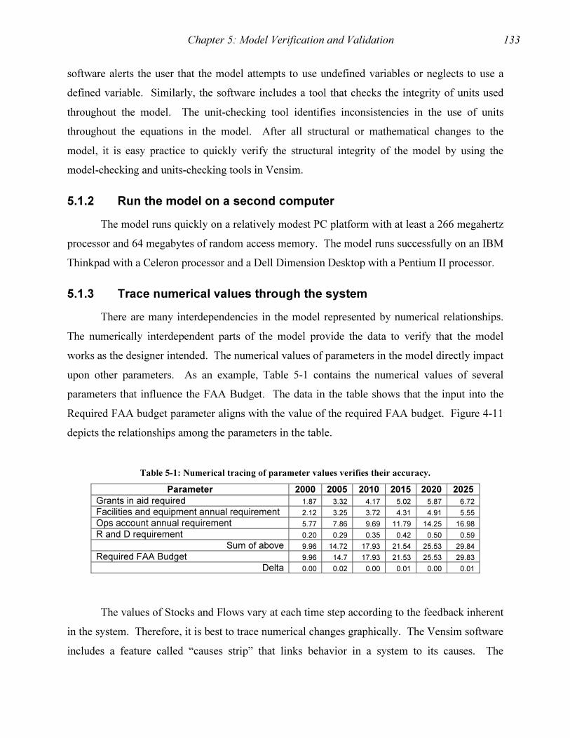
Chapter 5: Model Verification and Validation 133
software alerts the user that the model attempts to use undefined variables or neglects to use a
defined variable. Similarly, the software includes a tool that checks the integrity of units used
throughout the model. The unit-checking tool identifies inconsistencies in the use of units
throughout the equations in the model. After all structural or mathematical changes to the
model, it is easy practice to quickly verify the structural integrity of the model by using the
model-checking and units-checking tools in Vensim.
5.1.2 Run the model on a second computer
The model runs quickly on a relatively modest PC platform with at least a 266 megahertz
processor and 64 megabytes of random access memory. The model runs successfully on an IBM
Thinkpad with a Celeron processor and a Dell Dimension Desktop with a Pentium II processor.
5.1.3 Trace numerical values through the system
There are many interdependencies in the model represented by numerical relationships.
The numerically interdependent parts of the model provide the data to verify that the model
works as the designer intended. The numerical values of parameters in the model directly impact
upon other parameters. As an example, Table 5-1 contains the numerical values of several
parameters that influence the FAA Budget. The data in the table shows that the input into the
Required FAA budget parameter aligns with the value of the required FAA budget. Figure 4-11
depicts the relationships among the parameters in the table.
Table 5-1: Numerical tracing of parameter values verifies their accuracy.
Parameter 2000 2005 2010 2015 2020 2025 Grants in aid required 1.87 3.32 4.17 5.02 5.87 6.72
Facilities and equipment annual requirement 2.12 3.25 3.72 4.31 4.91 5.55
Ops account annual requirement 5.77 7.86 9.69 11.79 14.25 16.98
R and D requirement 0.20 0.29 0.35 0.42 0.50 0.59
Sum of above 9.96 14.72 17.93 21.54 25.53 29.84
Required FAA Budget 9.96 14.7 17.93 21.53 25.53 29.83
Delta 0.00 0.02 0.00 0.01 0.00 0.01
The values of Stocks and Flows vary at each time step according to the feedback inherent
in the system. Therefore, it is best to trace numerical changes graphically. The Vensim software
includes a feature called “causes strip” that links behavior in a system to its causes. The
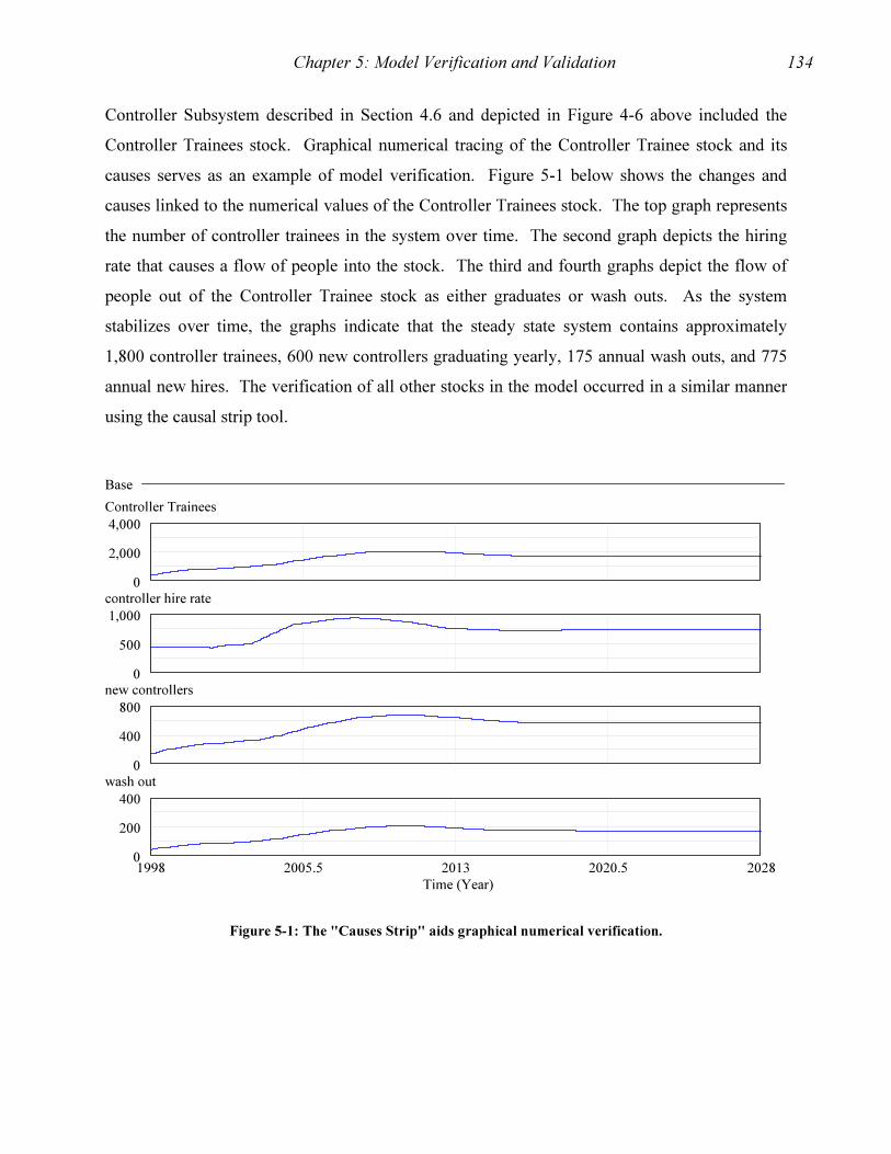
Chapter 5: Model Verification and Validation 134
Controller Subsystem described in Section 4.6 and depicted in Figure 4-6 above included the
Controller Trainees stock. Graphical numerical tracing of the Controller Trainee stock and its
causes serves as an example of model verification. Figure 5-1 below shows the changes and
causes linked to the numerical values of the Controller Trainees stock. The top graph represents
the number of controller trainees in the system over time. The second graph depicts the hiring
rate that causes a flow of people into the stock. The third and fourth graphs depict the flow of
people out of the Controller Trainee stock as either graduates or wash outs. As the system
stabilizes over time, the graphs indicate that the steady state system contains approximately
1,800 controller trainees, 600 new controllers graduating yearly, 175 annual wash outs, and 775
annual new hires. The verification of all other stocks in the model occurred in a similar manner
using the causal strip tool.
Base
Controller Trainees
4,000
2,000
0controller hire rate
1,000
500
0new controllers
800
400
0wash out
400
200
01998 2005.5 2013 2020.5 2028
Time (Year)
Figure 5-1: The "Causes Strip" aids graphical numerical verification.
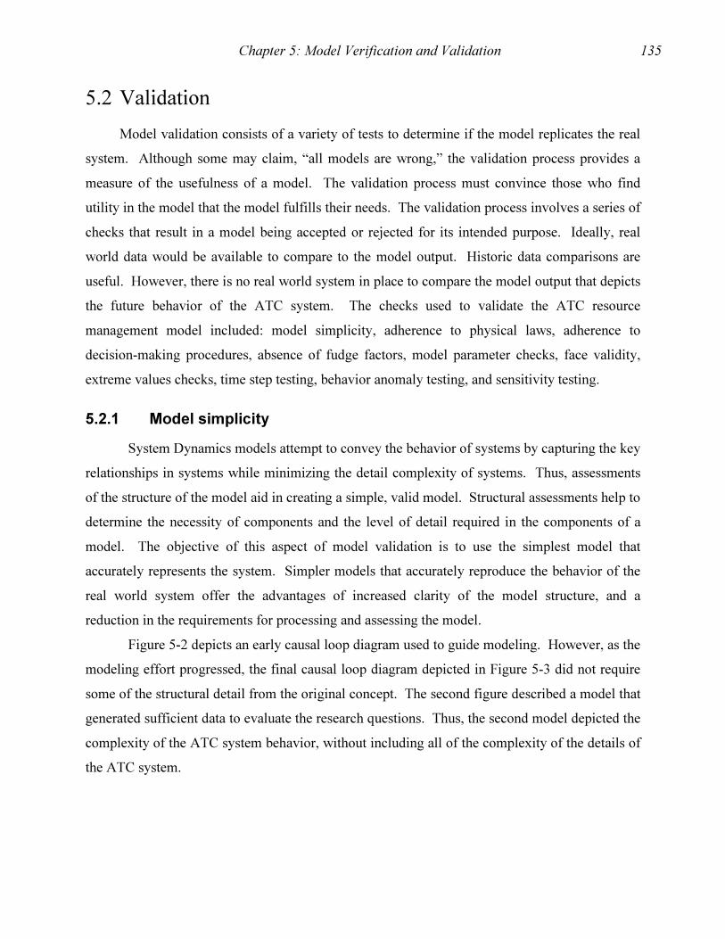
Chapter 5: Model Verification and Validation 135
5.2 Validation
Model validation consists of a variety of tests to determine if the model replicates the real
system. Although some may claim, “all models are wrong,” the validation process provides a
measure of the usefulness of a model. The validation process must convince those who find
utility in the model that the model fulfills their needs. The validation process involves a series of
checks that result in a model being accepted or rejected for its intended purpose. Ideally, real
world data would be available to compare to the model output. Historic data comparisons are
useful. However, there is no real world system in place to compare the model output that depicts
the future behavior of the ATC system. The checks used to validate the ATC resource
management model included: model simplicity, adherence to physical laws, adherence to
decision-making procedures, absence of fudge factors, model parameter checks, face validity,
extreme values checks, time step testing, behavior anomaly testing, and sensitivity testing.
5.2.1 Model simplicity
System Dynamics models attempt to convey the behavior of systems by capturing the key
relationships in systems while minimizing the detail complexity of systems. Thus, assessments
of the structure of the model aid in creating a simple, valid model. Structural assessments help to
determine the necessity of components and the level of detail required in the components of a
model. The objective of this aspect of model validation is to use the simplest model that
accurately represents the system. Simpler models that accurately reproduce the behavior of the
real world system offer the advantages of increased clarity of the model structure, and a
reduction in the requirements for processing and assessing the model.
Figure 5-2 depicts an early causal loop diagram used to guide modeling. However, as the
modeling effort progressed, the final causal loop diagram depicted in Figure 5-3 did not require
some of the structural detail from the original concept. The second figure described a model that
generated sufficient data to evaluate the research questions. Thus, the second model depicted the
complexity of the ATC system behavior, without including all of the complexity of the details of
the ATC system.
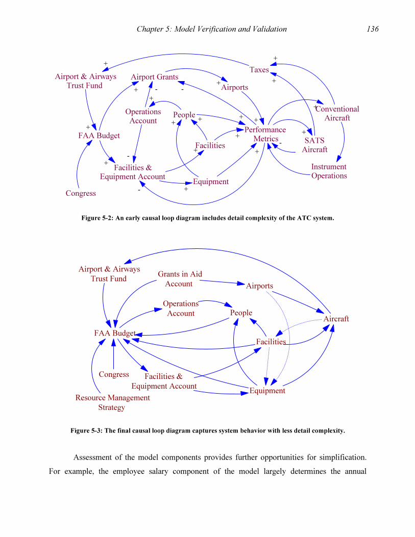
Chapter 5: Model Verification and Validation 136
OperationsAccount
Airport Grants
InstrumentOperations
Facilities &Equipment Account
FAA BudgetPerformance
Metrics
+
+
People
Congress
Airport & AirwaysTrust Fund
+
SATSAircraft
Airports+
+
Equipment
Facilities
+
+
+
+
++
Taxes
ConventionalAircraft
-
+
-
+
+
+
+
+
-
-
-
-
+
Figure 5-2: An early causal loop diagram includes detail complexity of the ATC system.
Airport & Airways
Trust Fund
Congress
FAA Budget
Airports
Facilities
People
Equipment
Aircraft
Resource Management
Strategy
Grants in Aid
Account
Operations
Account
Facilities &
Equipment Account
Figure 5-3: The final causal loop diagram captures system behavior with less detail complexity.
Assessment of the model components provides further opportunities for simplification.
For example, the employee salary component of the model largely determines the annual
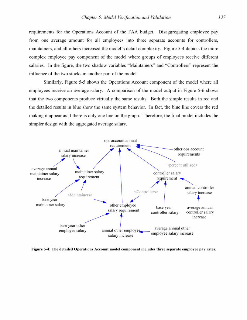
Chapter 5: Model Verification and Validation 137
requirements for the Operations Account of the FAA budget. Disaggregating employee pay
from one average amount for all employees into three separate accounts for controllers,
maintainers, and all others increased the model’s detail complexity. Figure 5-4 depicts the more
complex employee pay component of the model where groups of employees receive different
salaries. In the figure, the two shadow variables “Maintainers” and “Controllers” represent the
influence of the two stocks in another part of the model.
Similarly, Figure 5-5 shows the Operations Account component of the model where all
employees receive an average salary. A comparison of the model output in Figure 5-6 shows
that the two components produce virtually the same results. Both the simple results in red and
the detailed results in blue show the same system behavior. In fact, the blue line covers the red
making it appear as if there is only one line on the graph. Therefore, the final model includes the
simpler design with the aggregated average salary.
annual maintainer
salary increase
maintainer salary
requirement
base year
maintainer salary
average annualmaintainer salary
increase
<Controllers>
other ops account
requirements
ops account annual
requirement
<Maintainers>
<percent utilized>
annual controller
salary increase
controller salary
requirement
base year
controller salary
average annualcontroller salary
increase
annual other employee
salary increase
other employee
salary requirement
base year other
employee salaryaverage annual other
employee salary increase
Figure 5-4: The detailed Operations Account model component includes three separate employee pay rates.
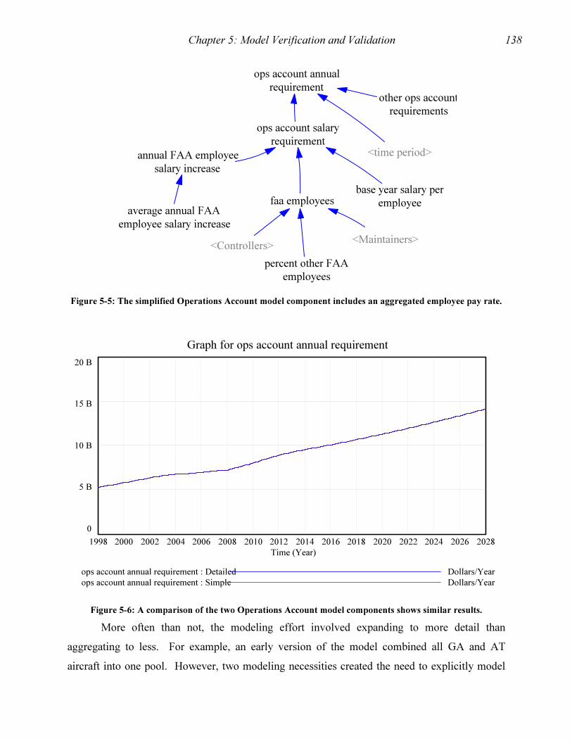
Chapter 5: Model Verification and Validation 138
faa employees
percent other FAA
employees
annual FAA employee
salary increase
ops account salary
requirement
base year salary per
employeeaverage annual FAA
employee salary increase
<Controllers>
other ops account
requirements
ops account annual
requirement
<Maintainers>
<time period>
Figure 5-5: The simplified Operations Account model component includes an aggregated employee pay rate.
Graph for ops account annual requirement
20 B
15 B
10 B
5 B
0
1998 2000 2002 2004 2006 2008 2010 2012 2014 2016 2018 2020 2022 2024 2026 2028
Time (Year)
ops account annual requirement : Detailed Dollars/Year
ops account annual requirement : Simple Dollars/Year
Figure 5-6: A comparison of the two Operations Account model components shows similar results.
More often than not, the modeling effort involved expanding to more detail than
aggregating to less. For example, an early version of the model combined all GA and AT
aircraft into one pool. However, two modeling necessities created the need to explicitly model

Chapter 5: Model Verification and Validation 139
both GA aircraft and AT aircraft as separate entities. First, the analysis of air traffic control
tower operations showed that the towers were non-homogenous. Subsequently, the model
required distinct GA and AT aircraft stocks to measure changes in aircraft populations that
influenced the numbers of control towers required in the system. Second, the conversion rates of
GA and AT aircraft into SATS aircraft differ. Therefore, the model uses two stocks to
distinguish between the flow of converted GA aircraft into SATS aircraft and the flow of
converted AT aircraft into SATS aircraft.
5.2.2 Adherence to Physical Laws
The model adheres to physical laws. All stocks of entities; such as control towers,
aircraft, and people; maintained positive or zero values throughout normal model runs and during
all validation procedures.
5.2.3 Adherence to Decision-making procedures
The model contains a user interface to allow for adjustments in the resource management
guidance input into the ATC system. The guidance imbeds decision-making into the model that
adjusts the flow of resources according to the desired resource management strategy. Within the
model, a variety of feedback occurs that corresponds to decision-making within the system. For
example, the FAA hired 430 people on average annually from FY1997 to FY2001 (Government
Accounting Office, 2002). The system adjusts the controller hiring rate based on the
requirements for controllers demanded by the ATC facilities in the system. As facilities open or
close, the requirement for controllers changes. Additionally, the number of controllers in the
system also changes based on retirements, early departures, and the flow of trainees. The
extreme values testing in section 5.2.7 included checks for adherence to proper decision-making
by all the feedback loops in Figure 5-3.
5.2.4 Absence of “fudge factors”
All parameters in the model correspond to real world values. The units used in the model
correspond with the stocks. All but two of the units in the model consist of the actual entities:
People, Towers, Centers, TRACONS, FSSs, Aircraft, Airports, Equipment, and Dollars. The
other two units include time, expressed as Years, and a non-unit descriptor, expressed as
Dimensionless. Some of the parameters express estimates of the feedback from one component

Chapter 5: Model Verification and Validation 140
of the model to another. For instance, the parameter “effect of people shortage on tax revenue”
causes a reduction of tax revenue when either the controllers or maintainer populations are at less
than 70% of the required manning level. The effect is an example of an estimate that
corresponds to a real world value, but the exact value is not known. The intent of using such
estimates is to capture the general relationships that cause feedback in the ATC system. To
disregard the relationship by not including it in the model would, by default, assign the value of
zero.
5.2.5 Model Parameter Checks
Although model parameters have meaning in the real world, the required accuracy of
parameter estimates depends on how sensitive the final policy recommendations are to the
particular estimate. Parameters embellish the flows into and out of the stocks. The importance
of individual parameters in the model varies according to their effect on the system behavior
relevant to decision-making.
Two techniques are useful for checking model parameters. The first technique is to ask
experts knowledgeable of the system to confirm the accuracy of the parameters. Experts from
the FAA provided several parameters for the People Submodel. The second technique is to use
partial model tests to isolate and evaluate parameters. Table 5-2 provides a list of all model
parameters, their values, units, origins, and the results of partial model tests. The entries in bold
font describe the results of the partial model tests on the submodel groupings in the lines below.
Blue font delineates the submodel groupings. Although experts provided some of the values,
most entries in the table are a result of calculations.
The results in Table 5-2 lead to several conclusions. First, when isolated, the parameters
that are constants cause no dynamic behavior in the system. All stocks remain at their initial
values during partial model tests involving only constants. However, when evaluated as
submodels, the groups of parameters in a submodel cause dynamic behavior in the model. In
particular, the Operations Account submodel has the most influence on the FAA budget due to
the exponential growth it causes. Conversely, the Controller and Maintainer submodels contain
balancing loops that seek stability. The Aircraft submodel grows or declines because of the
availability of resources in the system. Overall, all submodels exhibited valid behavior
throughout the partial model tests, described in black, bold font for each stock in each submodel.

Chapter 5: Model Verification and Validation 141
Table 5-2: Partial model tests are useful validation tools.
Value Units Origin
BUDGET SUBSYSTEM – exponential growth when all other variables held constant.
annual interest (interest on the unused portion of the Airport and Airways Trust Fund)
4% 1/Year Estimate
R and D requirement (2% of the FAA budget funds the Research and Development program.)
2% Dimensionless Calculation
time period (Adjusts units to account for a time period over which change occurs.)
1 1/Year Calculation
Operations Account – exponential growth when all other variables held constant.
base year salary (Base year salary from 1998 = $74,202 average for all FAA employees.)
74,202 Dollars/People Calculation
Average annual FAA employee salary increase ($8,879 annually (slope from 1998-2002 data))
8,879 (Dollars/People)/Year Calculation
percent other FAA employees (40% of FAA employees are inspectors and administrators. Therefore, 100/60 = 1.67, the multiplication factor to obtain the total number of employees.)
1.67 Dimensionless Calculation
other ops account requirements (Factor to multiply ops account salary figure by to obtain entire ops account requirement. 74% of ops account pays for salaries, the remaining 26% pays for rent, contracts, travel, and other services for employees.)
1.35 Dimensionless Calculation
Facilities and Equipment Account – linear growth or decline when all other variables held
constant.
radar eqpt avg annual cost ($90,000 per piece of radar-based ATC equipment is required from the F&E account annually)
90,000 Dollars/Equipment Calculation
GPS eqpt avg annual cost ($460,000 per piece of GPS-based ATC equipment is required from the F&E account annually)
460,000 Dollars/Equipment Calculation
FSS avg annual cost ($280,000 per FSS is required from the F&E account annually)
280,000 Dollars/FSSs Calculation
ga tower avg annual cost ($350,000 per GA tower is required from the F&E account annually)
350,000 Dollars/Towers Calculation
at tower avg annual cost ($420,000 per AT tower is required from the F&E account annually)
420,000 Dollars/Towers Calculation
ac tower avg annual cost ($1,010,000 per AC tower is required from the F&E account annually)
1,010,000 Dollars/Towers Calculation
TRACON avg annual cost ($670,000 per TRACON is required from the F&E account annually)
670,000 Dollars/TRACONs Calculation
center avg annual cost ($13,570,000 per Center is required from the F&E account annually)
13,570,000 Dollars/Centers Calculation
other facilities costs (All other facilities cost $361M in base year 1998 and include 19% of the F&E account)
361,000,000 Dollars Calculation
ramp increase in 01 and 02 ($450M increase to F&E account in 2001 and 2002)

Chapter 5: Model Verification and Validation 142
450,000,000 Dollars/Year Calculation
Operating cost growth factor (2% operating cost growth rate)
2 Year Estimate
Grants-in-Aid Account – linear growth when all other variables held constant.
average annual increase in Grants in Aid (estimate of the average annual increase in the Grants-in-Aid account is $170M annually)
170,000,000 Dollars/Year Calculation
base year grants in aid (The 1998 Grants in Aid account was $1.7B.)
170,000,000,000 Dollars Calculation
ramp increase in 2001 and 02 ($600M increase to Grants in Aid account in 2001 and 2002)
600,000,000 Dollars/Year Calculation
Airport and Airway Trust Fund – linear growth in aircraft when all other variables held
constant.
base year tax revenue per AC aircraft (Assume base year is avg of revenue from 1998-2003 calculated in part 4.7.5 in dissertation is $1,133,000.)
1,133,000 Dollars/Aircraft Calculation
avg annual increase in AC tax revenue (Assume average increase in taxes is $50,000 annually)
50,000 (Dollars/Aircraft)/Year Estimate
base year tax revenue per AT GA or SATS aircraft (Assume base year is $6,639 = avg of revenue from 1998-2003,)
6,639 Dollars/Aircraft Calculation
avg annual increase in AT GA or SATS tax revenue (Assume average increase in taxes is $300 annually)
300 (Dollars/Aircraft)/Year Estimate
AIRPORTS – linear growth or decline when all other variables held constant.
ramp for max annual airport conversions (The maximum number of nonSATS airports that can be converted to SATS airports annually. A RAMP function starting with 5 airports per year in 2010 and increasing by 5 airports annually until 2015.)
5 annually for 5 years Dimensionless Estimate
base year nonSATS airports (There were 2806 public use nonSATS airports in the US in the baseyear 1998 that were also potential candidates to become SATS airports due to their inclusion on the National Plan of Integrated Airport Systems (NPIAS) list.)
2,806 Airports Calculation
timeperiod for nonSATS airports (Assume 1 new airport is built annually from 1998 until 2010.)
1 Dimensionless Estimate
annual new nonSATS airports (Assume 1 new airport is built annually from 1998 until 2010.)
1 Airports/Year Estimate
first year for SATS airports (The first year a SATS airport becomes operational.)
2010 Year Estimate
SATS airport conversion cost (Assume it cost $2M to convert an airport to a SATS airport.)
2,000,000 Dollars/Airports Estimate
PEOPLE
Controllers – balancing behavior, seeks approx 19,300 when all other variables held
constant.
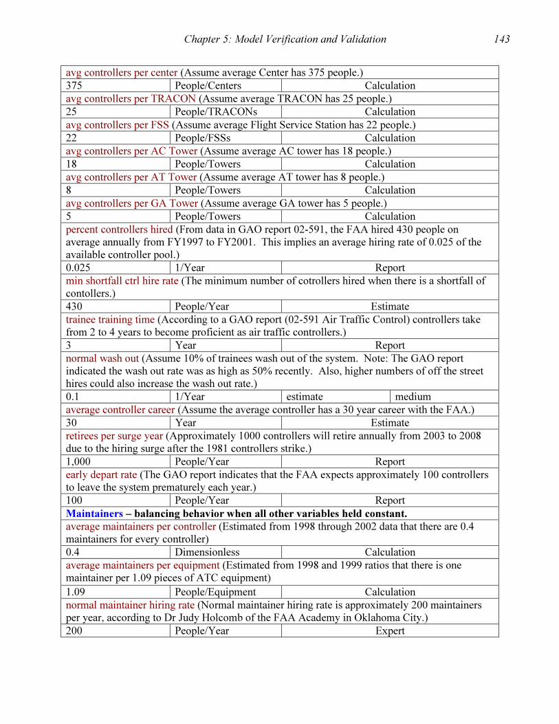
Chapter 5: Model Verification and Validation 143
avg controllers per center (Assume average Center has 375 people.)
375 People/Centers Calculation
avg controllers per TRACON (Assume average TRACON has 25 people.)
25 People/TRACONs Calculation
avg controllers per FSS (Assume average Flight Service Station has 22 people.)
22 People/FSSs Calculation
avg controllers per AC Tower (Assume average AC tower has 18 people.)
18 People/Towers Calculation
avg controllers per AT Tower (Assume average AT tower has 8 people.)
8 People/Towers Calculation
avg controllers per GA Tower (Assume average GA tower has 5 people.)
5 People/Towers Calculation
percent controllers hired (From data in GAO report 02-591, the FAA hired 430 people on average annually from FY1997 to FY2001. This implies an average hiring rate of 0.025 of the available controller pool.)
0.025 1/Year Report
min shortfall ctrl hire rate (The minimum number of cotrollers hired when there is a shortfall of contollers.)
430 People/Year Estimate
trainee training time (According to a GAO report (02-591 Air Traffic Control) controllers take from 2 to 4 years to become proficient as air traffic controllers.)
3 Year Report
normal wash out (Assume 10% of trainees wash out of the system. Note: The GAO report indicated the wash out rate was as high as 50% recently. Also, higher numbers of off the street hires could also increase the wash out rate.)
0.1 1/Year estimate medium
average controller career (Assume the average controller has a 30 year career with the FAA.)
30 Year Estimate
retirees per surge year (Approximately 1000 controllers will retire annually from 2003 to 2008 due to the hiring surge after the 1981 controllers strike.)
1,000 People/Year Report
early depart rate (The GAO report indicates that the FAA expects approximately 100 controllers to leave the system prematurely each year.)
100 People/Year Report
Maintainers – balancing behavior when all other variables held constant.
average maintainers per controller (Estimated from 1998 through 2002 data that there are 0.4 maintainers for every controller)
0.4 Dimensionless Calculation
average maintainers per equipment (Estimated from 1998 and 1999 ratios that there is one maintainer per 1.09 pieces of ATC equipment)
1.09 People/Equipment Calculation
normal maintainer hiring rate (Normal maintainer hiring rate is approximately 200 maintainers per year, according to Dr Judy Holcomb of the FAA Academy in Oklahoma City.)
200 People/Year Expert

Chapter 5: Model Verification and Validation 144
maintainer trainee training time (According to Dr Holcomb at the FAA Academy, it takes about 2 years for a system maintainer to become fully proficient.)
2 Year Expert
average maintainer career (Average maintainer career is 35+ years according to Dr Holcomb, FAA Academy.)
35 Year Expert
accelerated retirement due to average age (Since average maintainer career is 35+ years and the average age of maintainers is 47 in 2002, there will be an accelerated retirement rate until the average age of the workforce delcines. This variable causes a linear decline in the retirment rate for 20 years.)
-0.1 Year Expert
FACILITIES AND EQUIPMENT
Centers, TRACONS, FSSs – linear growth or decline when all other variables held
constant.
interval between center consolidations (Assume two centers consolidate every 7 years.)
7 Year Estimate
interval between tracon consolidations (Assume two TRACONs consolidate every 10 years.)
10 Year Estimate
normal fss construction rate (Assume two new FSSs built per year.)
2 FSSs/Year Estimate
AC Control Towers – linear growth when all other variables held constant.
normal ac tower construction rate (Assume 1 new towers opens every four years.)
0.25 Towers/Year Calculation
normal ac tower closure rate (Assume 1 tower closes every 8 years.)
0.125 Towers/Year Calculation
AT Control Towers – linear growth when all other variables held constant.
normal at tower construction rate (Assume 1 new towers opens every two years.)
0.5 Towers/Year Calculation
normal at tower closure rate (Assume 1 tower closes every 4 years.)
0.25 Towers/Year Calculation
GA Control Towers – linear growth when all other variables held constant.
normal ga tower construction rate (Assume 1.5 new towers open every two years.)
1.5 Towers/Year Calculation
normal ga tower closure rate (Assume 0.5 tower closes every year.)
0.5 Towers/Year Calculation
normal ga tower closure rate (Assume 0.5 tower closes every year.)
0.5 Towers/Year Calculation
Radar-based Equipment – linear growth when all other variables held constant.
radar equipt replacement rate per AC tower (AC Towers annually require 0.52 replacement pieces of radar-based equipment to replace ILS, ASR-T, ARTS, and VASI.)
0.52 Equipt/Towers/Year Calculation
radar equipt replacement rate per AT tower (AT Towers annually require 0.37 replacement pieces of radar-based equipment to replace ILS, ASR-T, ARTS, and VASI.)
0.37 Equipt/Towers/Year Calculation
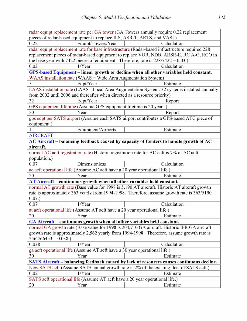
Chapter 5: Model Verification and Validation 145
radar equipt replacement rate per GA tower (GA Towers annually require 0.22 replacement pieces of radar-based equipment to replace ILS, ASR-T, ARTS, and VASI.)
0.22 Equipt/Towers/Year Calculation
radar equipt replacement rate for base infrastructure (Radar-based infrastructure required 228 replacement pieces of radar-based equipment to replace VOR, NDB, ARSR-E, RC A-G, RCO in the base year with 7422 pieces of equipment. Therefore, rate is 228/7422 = 0.03.)
0.03 1/Year Calculation
GPS-based Equipment – linear growth or decline when all other variables held constant.
WAAS installation rate (WAAS = Wide Area Augmentation System)
5 Eqpt/Year Estimate
LAAS installation rate (LAAS - Local Area Augmentation System: 32 systems installed annually from 2002 until 2006 and thereafter when directed as a resource priority)
32 Eqpt/Year Report
GPS equipment lifetime (Assume GPS equipment lifetime is 20 years.)
20 Year Report
gps eqpt per SATS airport (Assume each SATS airport contributes a GPS-based ATC piece of equipment.)
1 Equipment/Airports Estimate
AIRCRAFT
AC Aircraft – balancing feedback caused by capacity of Centers to handle growth of AC
aircraft.
normal AC acft registration rate (Historic registration rate for AC acft is 7% of AC acft population.)
0.07 Dimensionless Calculation
ac acft operational life (Assume AC acft have a 20 year operational life.)
20 Year Estimate
AT Aircraft – continuous growth when all other variables held constant.
normal AT growth rate (Base value for 1998 is 5,190 AT aircraft. Historic AT aircraft growth rate is approximately 363 yearly from 1994-1998. Therefore, assume growth rate is 363/5190 = 0.07.)
0.07 1/Year Calculation
at acft operational life (Assume AT acft have a 20 year operational life.)
20 Year Estimate
GA Aircraft – continuous growth when all other variables held constant.
normal GA growth rate (Base value for 1998 is 204,710 GA aircraft. Historic IFR GA aircraft growth rate is approximately 2,562 yearly from 1994-1998. Therefore, assume growth rate is 2562/66453 = 0.038.)
0.038 1/Year Calculation
ga acft operational life (Assume AT acft have a 30 year operational life.)
30 Year Estimate
SATS Aircraft – balancing feedback caused by lack of resources causes continuous decline.
New SATS acft (Assume SATS annual growth rate is 2% of the existing fleet of SATS acft.)
0.02 1/Year Estimate
SATS acft operational life (Assume AT acft have a 20 year operational life.)
20 Year Estimate
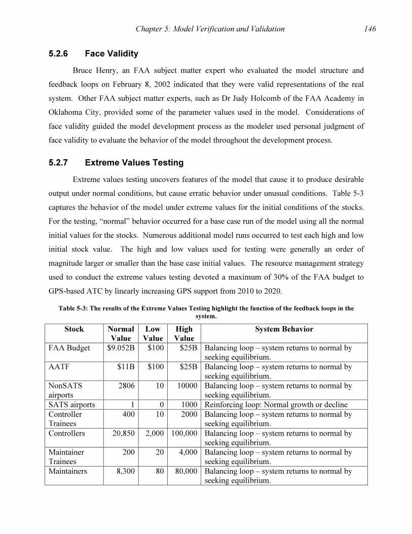
Chapter 5: Model Verification and Validation 146
5.2.6 Face Validity
Bruce Henry, an FAA subject matter expert who evaluated the model structure and
feedback loops on February 8, 2002 indicated that they were valid representations of the real
system. Other FAA subject matter experts, such as Dr Judy Holcomb of the FAA Academy in
Oklahoma City, provided some of the parameter values used in the model. Considerations of
face validity guided the model development process as the modeler used personal judgment of
face validity to evaluate the behavior of the model throughout the development process.
5.2.7 Extreme Values Testing
Extreme values testing uncovers features of the model that cause it to produce desirable
output under normal conditions, but cause erratic behavior under unusual conditions. Table 5-3
captures the behavior of the model under extreme values for the initial conditions of the stocks.
For the testing, “normal” behavior occurred for a base case run of the model using all the normal
initial values for the stocks. Numerous additional model runs occurred to test each high and low
initial stock value. The high and low values used for testing were generally an order of
magnitude larger or smaller than the base case initial values. The resource management strategy
used to conduct the extreme values testing devoted a maximum of 30% of the FAA budget to
GPS-based ATC by linearly increasing GPS support from 2010 to 2020.
Table 5-3: The results of the Extreme Values Testing highlight the function of the feedback loops in the
system.
Stock Normal
Value
Low
Value
High
Value
System Behavior
FAA Budget $9.052B $100 $25B Balancing loop – system returns to normal by seeking equilibrium.
AATF $11B $100 $25B Balancing loop – system returns to normal by seeking equilibrium.
NonSATS airports
2806 10 10000 Balancing loop – system returns to normal by seeking equilibrium.
SATS airports 1 0 1000 Reinforcing loop: Normal growth or decline
Controller Trainees
400 10 2000 Balancing loop – system returns to normal by seeking equilibrium.
Controllers 20,850 2,000 100,000 Balancing loop – system returns to normal by seeking equilibrium.
Maintainer Trainees
200 20 4,000 Balancing loop – system returns to normal by seeking equilibrium.
Maintainers 8,300 80 80,000 Balancing loop – system returns to normal by seeking equilibrium.
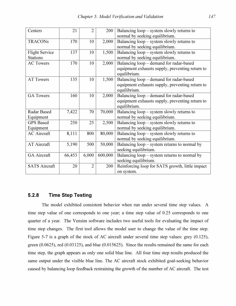
Chapter 5: Model Verification and Validation 147
Centers 21 2 200 Balancing loop – system slowly returns to normal by seeking equilibrium.
TRACONs 170 10 2,000 Balancing loop – system slowly returns to normal by seeking equilibrium.
Flight Service Stations
137 10 1,500 Balancing loop – system slowly returns to normal by seeking equilibrium.
AC Towers 170 10 2,000 Balancing loop – demand for radar-based equipment exhausts supply, preventing return to equilibrium.
AT Towers 135 10 1,500 Balancing loop – demand for radar-based equipment exhausts supply, preventing return to equilibrium.
GA Towers 160 10 2,000 Balancing loop – demand for radar-based equipment exhausts supply, preventing return to equilibrium.
Radar Based Equipment
7,422 70 70,000 Balancing loop – system slowly returns to normal by seeking equilibrium.
GPS Based Equipment
250 25 2,500 Balancing loop – system slowly returns to normal by seeking equilibrium.
AC Aircraft 8,111 800 80,000 Balancing loop – system slowly returns to normal by seeking equilibrium.
AT Aircraft 5,190 500 50,000 Balancing loop – system returns to normal by seeking equilibrium.
GA Aircraft 66,453 6,000 600,000 Balancing loop – system returns to normal by seeking equilibrium.
SATS Aircraft 20 2 200 Reinforcing loop for SATS growth, little impact on system.
5.2.8 Time Step Testing
The model exhibited consistent behavior when run under several time step values. A
time step value of one corresponds to one year; a time step value of 0.25 corresponds to one
quarter of a year. The Vensim software includes two useful tools for evaluating the impact of
time step changes. The first tool allows the model user to change the value of the time step.
Figure 5-7 is a graph of the stock of AC aircraft under several time step values: grey (0.125),
green (0.0625), red (0.03125), and blue (0.015625). Since the results remained the same for each
time step, the graph appears as only one solid blue line. All four time step results produced the
same output under the visible blue line. The AC aircraft stock exhibited goal-seeking behavior
caused by balancing loop feedback restraining the growth of the number of AC aircraft. The test
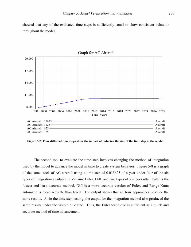
Chapter 5: Model Verification and Validation 148
showed that any of the evaluated time steps is sufficiently small to show consistent behavior
throughout the model.
Graph for AC Aircraft
20,000
17,000
14,000
11,000
8,000
1998 2000 2002 2004 2006 2008 2010 2012 2014 2016 2018 2020 2022 2024 2026 2028
Time (Year)
AC Aircraft : 15625 Aircraft
AC Aircraft : 3125 Aircraft
AC Aircraft : 625 Aircraft
AC Aircraft : 125 Aircraft
Figure 5-7: Four different time steps show the impact of reducing the size of the time step in the model.
The second tool to evaluate the time step involves changing the method of integration
used by the model to advance the model in time to create system behavior. Figure 5-8 is a graph
of the same stock of AC aircraft using a time step of 0.015625 of a year under four of the six
types of integration available in Vensim: Euler, Diff, and two types of Runge-Kutta. Euler is the
fastest and least accurate method, Diff is a more accurate version of Euler, and Runge-Kutta
automatic is more accurate than fixed. The output shows that all four approaches produce the
same results. As in the time step testing, the output for the integration method also produced the
same results under the visible blue line. Thus, the Euler technique is sufficient as a quick and
accurate method of time advancement.

Chapter 5: Model Verification and Validation 149
Graph for AC Aircraft
20,000
17,000
14,000
11,000
8,000
1998 2000 2002 2004 2006 2008 2010 2012 2014 2016 2018 2020 2022 2024 2026 2028
Time (Year)
AC Aircraft : RK4Fixed Aircraft
AC Aircraft : RK4Auto Aircraft
AC Aircraft : Diff Aircraft
AC Aircraft : Euler Aircraft
Figure 5-8: Four different time advancing integration techniques all produce the same results.
5.2.9 Behavior Reproduction Testing
Behavior reproduction testing is an attempt to model past system behavior to reproduce
historical data generated by real-world performance of the system. Table 5-4 below contains
actual and estimated initial values of the stocks in the ATC system in 1991. Table 5-5 below
contains additional initial values for parameters in the model. The 1991 Facilities and
Equipment values in Table 5-5 result from the formula: 1991 values = (1991 FAA Budget/1998
FAA Budget)*(1998 Value). The values in both tables define the initial conditions set in the
model to conduct the behavior reproduction test.
Table 5-4: Initial stock values for 1991 provide a basis for behavior reproduction testing.
Stock Initial Values 1991
Value
1998
Value
FAA Budget $7.732B $9.052B
AATF – estimate $9.0B $11B
NonSATS airports – estimate 2,550 2,806
SATS airports 0 1
Controller Trainees – estimate 500 400
Controllers 24,000 20,850

Chapter 5: Model Verification and Validation 150
Maintainer Trainees – estimate 160 200
Maintainers 6,600 8,300
Centers 24 21
TRACONs - estimate 180 170
Flight Service Stations – estimate 110 137
AC Towers – estimate 160 170
AT Towers – estimate 140 135
GA Towers – estimate 125 160
Radar Based Equipment – estimate 7,500 7,422
GPS Based Equipment – estimate 5 250
AC Aircraft 6,054 8,111
AT Aircraft 5,800 5,190
GA Aircraft – estimate 65,000 66,453
SATS Aircraft 0 20
Table 5-5: Initial parameter values for 1991 provide a basis for behavior reproduction testing.
Parameter Initial Values 1991 Value 1998 Value
base year salary - estimate $44,852 $64,591
Radar eqpt avg annual cost - estimate $76,500 $90,000
GPS eqpt avg annual cost – estimate $391,000 $460,000
FSS avg annual cost – estimate $238,000 $280,000
ga tower avg annual cost – estimate $297,500 $350,000
at tower avg annual cost – estimate $357,000 $420,000
ac tower avg annual cost – estimate $858,500 $1,010,000
TRACON avg annual cost – estimate $569,500 $670,000
center avg annual cost – estimate $11,534,500 $13,570,000
Other facilities costs – estimate $307M $361M
Base year grants in aid $1.6B $1.7B
Table 5-6 below contains the results of the behavior reproduction testing. The left
justified Grants, Ops, F&E, and Total rows show the historical expenditures of the FAA from
1991 to 2002. The right justified “Model” rows show the output of the model for the same time
period. The four figures below the table graphically depict the comparison of the model
behavior to the historic behavior of the system. The graphs indicate that the model provides a
valid representation of the real world system. Table 5-7 shows the results of statistical t-tests to
determine if the model and historical distributions were from the same distribution. In each case,
the hypothesis that the distributions differed was rejected, thus reinforcing the accuracy of the
model’s ability to reproduce past behavior.

Chapter 5: Model Verification and Validation 151
Table 5-6: The rows under the actual data contain the model data for the same time period.
Type 1991 1992 1993 1994 1995 1996 1998 1999 2000 2001 2002 Grants $1,600 1,900 2,050 1,690 2,161 2,214 1,700 1,950 1,896 3,193 3,300
Model 1,600 1,722 1,840 1,960 2,080 2,200 2,440 2,560 2,680 3,400 3,520
Ops 4,037 4,360 4,538 4,581 4,583 4,643 5,253 5,586 5,958 6,603 7,091
Model 3,827 4,066 4,331 4,611 4,897 5,180 5,719 5,976 6,231 6,491 6,763
F&E 2,095 2,394 2,350 2,120 2,033 1,875 1,900 2,121 2,034 2,651 2,914
Model 1,512 1,559 1,605 1,651 1,698 1,744 1,837 1,884 1,930 2,427 2,474
Total 7,732 8,654 8,938 8,391 8,777 8,732 9,052 9,657 9,888 12,447 13,305
Model 7,079 7,491 7,932 8,388 8,849 9,307 10,190 10,620 11,050 12,560 13,010
(Sources: 1998-2002 FAA, 2002a; 1991-1996: FAA; 1997 not available.)
Table 5-7: Statistical t-tests showed that the model reproduces the historical data when T>t.
t(9, 0.025) = 2.26 Grants in Aid Operations Facilities & Eqpt Total
Calculated T statistic 4.50 8.92 2.76 6.67
Same Distribution Yes Yes Yes Yes
$0
$500
$1,000
$1,500
$2,000
$2,500
$3,000
$3,500
$4,000
1991 1992 1993 1994 1995 1996 1998 1999 2000 2001 2002
Year
$M
Actual
M odel
Figure 5-9: The historic Grants-in-Aid account shows more variability than the model.

Chapter 5: Model Verification and Validation 152
0
1,000
2,000
3,000
4,000
5,000
6,000
7,000
8,000
1991 1992 1993 1994 1995 1996 1998 1999 2000 2001 2002
Year
$M
Actual
Model
Figure 5-10: The actual and modeled Operations Account show similar trends.
0
500
1,000
1,500
2,000
2,500
3,000
3,500
1991 1992 1993 1994 1995 1996 1998 1999 2000 2001 2002
Year
$M
Actual
Model
Figure 5-11: The historic Facilities and Equipment Account shows more variability than the model.
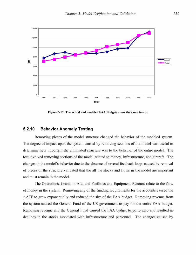
Chapter 5: Model Verification and Validation 153
0
2,000
4,000
6,000
8,000
10,000
12,000
14,000
1991 1992 1993 1994 1995 1996 1998 1999 2000 2001 2002
Year
$M
Actual
Model
Figure 5-12: The actual and modeled FAA Budgets show the same trends.
5.2.10 Behavior Anomaly Testing
Removing pieces of the model structure changed the behavior of the modeled system.
The degree of impact upon the system caused by removing sections of the model was useful to
determine how important the eliminated structure was to the behavior of the entire model. The
test involved removing sections of the model related to money, infrastructure, and aircraft. The
changes in the model’s behavior due to the absence of several feedback loops caused by removal
of pieces of the structure validated that the all the stocks and flows in the model are important
and must remain in the model.
The Operations, Grants-in-Aid, and Facilities and Equipment Account relate to the flow
of money in the system. Removing any of the funding requirements for the accounts caused the
AATF to grow exponentially and reduced the size of the FAA budget. Removing revenue from
the system caused the General Fund of the US government to pay for the entire FAA budget.
Removing revenue and the General Fund caused the FAA budget to go to zero and resulted in
declines in the stocks associated with infrastructure and personnel. The changes caused by

Chapter 5: Model Verification and Validation 154
removing sections of the system associated with the flow of money indicate that the sections all
play important roles in the model.
Removing the parts of the system associated with infrastructure also caused changes to
the system behavior. The removal of airports from the system prevented the expansion of the
pool of SATS aircraft and prevented the construction of SATS airports. Otherwise, the system
behaved normally because the model only includes nontowered public use airports. However,
the airports stocks are important for the growth of the SATS. Removing Centers, TRACONs,
Flight Service Stations, and Control Towers caused continuous reductions in the stocks of
revenue, airports, personnel and all aircraft except SATS aircraft. Removing radar-based or
GPS-based equipment caused an immediate decline in the population of all aircraft stocks.
Subsequently, the revenue and infrastructure stocks declined as well.
5.2.11 Sensitivity Analysis
The sensitivity of the behavior of the modeled ATC system varies with each of the
parameters in the model. If a parameter has a large influence on the range of behavior of the
system, then it is important to establish the accuracy of the parameter to increase the validity of
the model. The Vensim software contains procedures to conduct sensitivity testing using the
Monte Carlo approach. The approach involves inputting randomly generated parameter values
according to a selected probability distribution and a range of values for one or more parameters
in the model. The approach also involves running 200 simulations using the randomly generated
values, and then plotting the output within confidence bounds. The procedure is useful to
determine how changes in estimates or assumptions cause changes in the numerical and
graphical output of the model.
Table 5-8 below summarizes the results of the numerical sensitivity analysis. The results
show that several key parameters can influence the size of the AATF. For all sensitivity runs,
the modeled variables changed according to a random uniform distribution. For the runs below,
the ATC system resource managers maintained the current radar-based system with a small
annual investment in GPS equipment. Therefore, the runs below reflect the impact of the
variable changes on the continuance of the current ATC system into the future with no
significant increase in investment in the GPS-based approach to ATC. The determination of
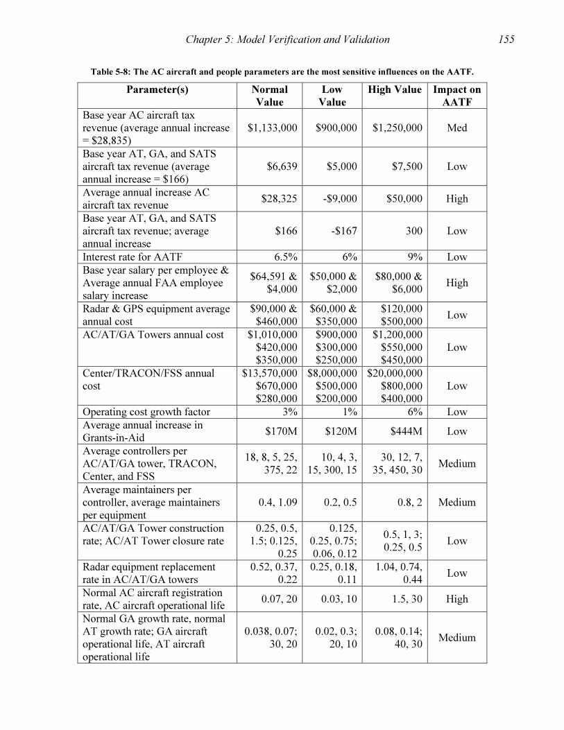
Chapter 5: Model Verification and Validation 155
Table 5-8: The AC aircraft and people parameters are the most sensitive influences on the AATF.
Parameter(s) Normal
Value
Low
Value
High Value Impact on
AATF
Base year AC aircraft tax revenue (average annual increase = $28,835)
$1,133,000 $900,000 $1,250,000 Med
Base year AT, GA, and SATS aircraft tax revenue (average annual increase = $166)
$6,639 $5,000 $7,500 Low
Average annual increase AC aircraft tax revenue
$28,325 -$9,000 $50,000 High
Base year AT, GA, and SATS aircraft tax revenue; average annual increase
$166 -$167 300 Low
Interest rate for AATF 6.5% 6% 9% Low
Base year salary per employee & Average annual FAA employee salary increase
$64,591 & $4,000
$50,000 & $2,000
$80,000 & $6,000
High
Radar & GPS equipment average annual cost
$90,000 & $460,000
$60,000 & $350,000
$120,000 $500,000
Low
AC/AT/GA Towers annual cost $1,010,000 $420,000$350,000
$900,000 $300,000 $250,000
$1,200,000$550,000$450,000
Low
Center/TRACON/FSS annual cost
$13,570,000$670,000$280,000
$8,000,000 $500,000 $200,000
$20,000,000$800,000$400,000
Low
Operating cost growth factor 3% 1% 6% Low
Average annual increase in Grants-in-Aid
$170M $120M $444M Low
Average controllers per AC/AT/GA tower, TRACON, Center, and FSS
18, 8, 5, 25, 375, 22
10, 4, 3, 15, 300, 15
30, 12, 7, 35, 450, 30
Medium
Average maintainers per controller, average maintainers per equipment
0.4, 1.09 0.2, 0.5 0.8, 2 Medium
AC/AT/GA Tower construction rate; AC/AT Tower closure rate
0.25, 0.5, 1.5; 0.125,
0.25
0.125, 0.25, 0.75; 0.06, 0.12
0.5, 1, 3; 0.25, 0.5
Low
Radar equipment replacement rate in AC/AT/GA towers
0.52, 0.37, 0.22
0.25, 0.18, 0.11
1.04, 0.74, 0.44
Low
Normal AC aircraft registration rate, AC aircraft operational life
0.07, 20 0.03, 10 1.5, 30 High
Normal GA growth rate, normal AT growth rate; GA aircraft operational life, AT aircraft operational life
0.038, 0.07; 30, 20
0.02, 0.3; 20, 10
0.08, 0.14; 40, 30
Medium

Chapter 5: Model Verification and Validation 156
high, medium, or low impact resulted from a subjective evaluation of the relative effect of each
parameter.
The sensitivity graphs below are representative of the types of results recorded in Table
5-8 above. The first two figures Figure 5-13 and Figure 5-14 show that the AATF is most
sensitive to the tax revenue generated by AC aircraft and the salaries of FAA employees. Figure
5-13 indicates that there is the potential for a great deal of uncertainty in the AATF caused by
variations in the amount of revenue generated by AC aircraft. The output indicates how much
the AATF may change when the base year tax revenue for AC aircraft randomly varies from
$900,000 to $1,250,000 and the average annual increase in AC tax revenue remains fixed at
$28,325. The unusual shape of the output indicates a relationship with the accelerated
retirements of controllers and maintainers during the first 20 years of the evaluated time period.
Figure 5-14 indicates that FAA salaries may cause the AATF to increase exponentially under
some conditions. The output indicates how much the AATF may change when FAA employee
annual salaries vary from $50,000 to $80,000 and salary increases vary from $2,000 to $6,000.
Employee salaries account for about 40% of the entire FAA budget; accordingly, the AATF is
very sensitive to adjustments in salaries.
The third and fourth figures below indicate that the AATF is moderately sensitive to
potential variations in the number of Maintainers in the ATC system and to variations in the
AATF interest rate. The output in Figure 5-15 indicates how much the AATF may change when
average Maintainers per controller and Maintainers per piece of equipment varies from 0.2 to 0.8
and 0.5 to 2.0. The system is very sensitive initially until narrowing to a tighter band of values at
approximately 2010. Figure 5-16 shows how the AATF is not very sensitive to variations in the
interest rate from 6% to 9%, indicated by the narrow band of potential values.
The fifth and final sensitivity graph shows that the AATF is barely sensitive to potential
variations in the tax revenue collected for AT, GA, and SATS aircraft. The output in Figure 5-17
indicates how much the AATF may change when the base year tax revenue for AT, GA, and
SATS aircraft randomly varies from $5,000 to $7,500 and the average annual increase in AT,
GA, and SATS tax revenue remains fixed at $166. Revenue for the AATF from AT and GA
aircraft only accounts for approximately 5% of the fund, thus, the AATF shows little sensitivity
to variations in the AT, GA, and SATS revenue.
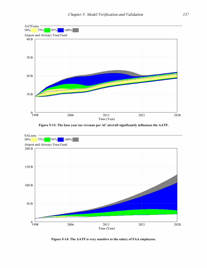
Chapter 5: Model Verification and Validation 157
AATFsens
50% 75% 95% 100%
Airport and Airways Trust Fund
40 B
30 B
20 B
10 B
01998 2006 2013 2021 2028
Time (Year)
Figure 5-13: The base year tax revenue per AC aircraft significantly influences the AATF.
SALsens
50% 75% 95% 100%
Airport and Airways Trust Fund
200 B
150 B
100 B
50 B
01998 2006 2013 2021 2028
Time (Year)
Figure 5-14: The AATF is very sensitive to the salary of FAA employees.
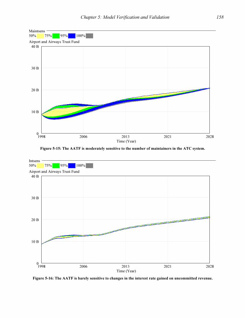
Chapter 5: Model Verification and Validation 158
Maintsens
50% 75% 95% 100%
Airport and Airways Trust Fund
40 B
30 B
20 B
10 B
01998 2006 2013 2021 2028
Time (Year)
Figure 5-15: The AATF is moderately sensitive to the number of maintainers in the ATC system.
Intsens
50% 75% 95% 100%
Airport and Airways Trust Fund
40 B
30 B
20 B
10 B
01998 2006 2013 2021 2028
Time (Year)
Figure 5-16: The AATF is barely sensitive to changes in the interest rate gained on uncommitted revenue.

Chapter 5: Model Verification and Validation 159
ATsens
50% 75% 95% 100%
Airport and Airways Trust Fund
40 B
30 B
20 B
10 B
01998 2006 2013 2021 2028
Time (Year)
Figure 5-17: The base year tax revenue per AT, GA, and SATS aircraft has little influence on the AATF.
5.3 Summary
The verification and validation procedures discussed above provide evidence that the ATC
Resource Management Model provides accurate and realistic results. The units in the model are
consistent and the numerical relationships are sound. The model has adequate detail complexity
and adheres to physical laws. The parameters in the model are reasonable and they create
intuitively correct behavior when replaced with extreme values. The model structure has face
validity; it exhibits normal behavior under various time steps and integration techniques. The
model generated reasonable results when reproducing ATC system behavior in the 1990s.
Finally, sensitivity analysis identified those parts of the model that have the greatest potential to
influence the results. The next chapter will describe the application of the model and the results
derived from it.

160
Chapter six presents a discussion of the results of the simulation and the analysis of the
three scenarios used to address the research questions. The first section presents an overview of
the three scenarios. The second section presents the base case conditions in the first scenario
when the resource management strategies support an ATC system continuing to operate as a
primarily radar-based system. The third section presents the resource management conditions
that cause the system to undergo an intentional transition toward the GPS-based approach to
ATC in the second scenario. The fourth section presents a resource management strategy
designed to create a balanced combination of both radar- and GPS-based ATC in the third
scenario.
The intent of this chapter is to illuminate the evidence and interpret it so as to arrive at the
proper conclusion. Specifically, the simulation and analysis should lead to a determination of
what air traffic control resource management strategy will support the future needs of the SATS
and create adequate tax revenue to fund the FAA. The development of the model in chapter four
and validation of the model in chapter five indicated that the resources generated by the AATF
are necessary to support SATS and provide money to run the FAA.
Essentially, the adequacy of the revenue generated for the AATF determines if the system
will be viable. The amount of money generated under each resource management scenario will
serve as a measure of viability. The strategy is viable if the amount of FAA funding required
from the General Fund does not exceed 20% of the FAA budget. The other two key variables
used to evaluate the merit of each resource management strategy are the numbers of SATS
aircraft and airports. Other metrics useful to understand and interpret the behavior of the system
include: the ratio of aircraft to airports, the control tower growth rate, the distribution of funds
across the major accounts of the FAA budget, the amount of money appropriated by Congress
for the FAA, and the conversion of public use airports into SATS airports.
Chapter 6: Simulation, Analysis, and Results
Chapter 6: Simulation, Analysis, and Results 161
6.1 Three ATC Scenarios
The valid model is useful to investigate the behavior of the ATC system with respect to
two primary influences. The first influence, an endogenous influence, alters system behavior due
to feedback from the values of the stocks within the system. For example, the AATF provides
funds to the FAA budget to pay for air traffic control towers. Changes to the population of air
traffic control towers influences the population of aircraft in the system. Subsequently, changes
in the aircraft population causes changes in the taxes collected for the AATF, which changes the
budget for control towers. Through feedback loops, the system behaves in a manner that seeks
growth and balance. The second influence, an exogenous influence, alters system behavior
because of management intervention to adjust the flow of dollar resources that pay for facilities,
equipment, and airports. For example, the desired level of support for GPS-based ATC causes
changes in the stocks of radar-based ATC facilities and equipment, which ripples through the
system by means of feedback loops.
In the model, managers distribute resources to support the radar-based or GPS-based
approach to ATC. The purpose of modeling the two influences is to determine what air traffic
control resource management strategy will support the future needs of the Small Aircraft
Transportation System and create adequate tax revenue to fund the Federal Aviation
Administration. The exogenous influences of the resource management strategy set the stage for
three scenarios that the model supports. The endogenous influences of the feedback loops
among the stocks in the system generate behavior that provides information to evaluate the best
resource management strategy.
6.1.1 Scenario 1: Maintain the Radar-Based System
The first resource management strategy is to maintain the current ratio of spending for
radar-based ATC and GPS-based ATC airports, equipment, and facilities.
Figure 6-1 depicts the continuation of the current resources management practices in the
first scenario that consist of providing GPS related funding to purchase only GPS-based ATC
equipment. Radar-based equipment receives 93% percent of all money provided for equipment.
Airports and facilities receive funding only for radar-based ATC requirements.
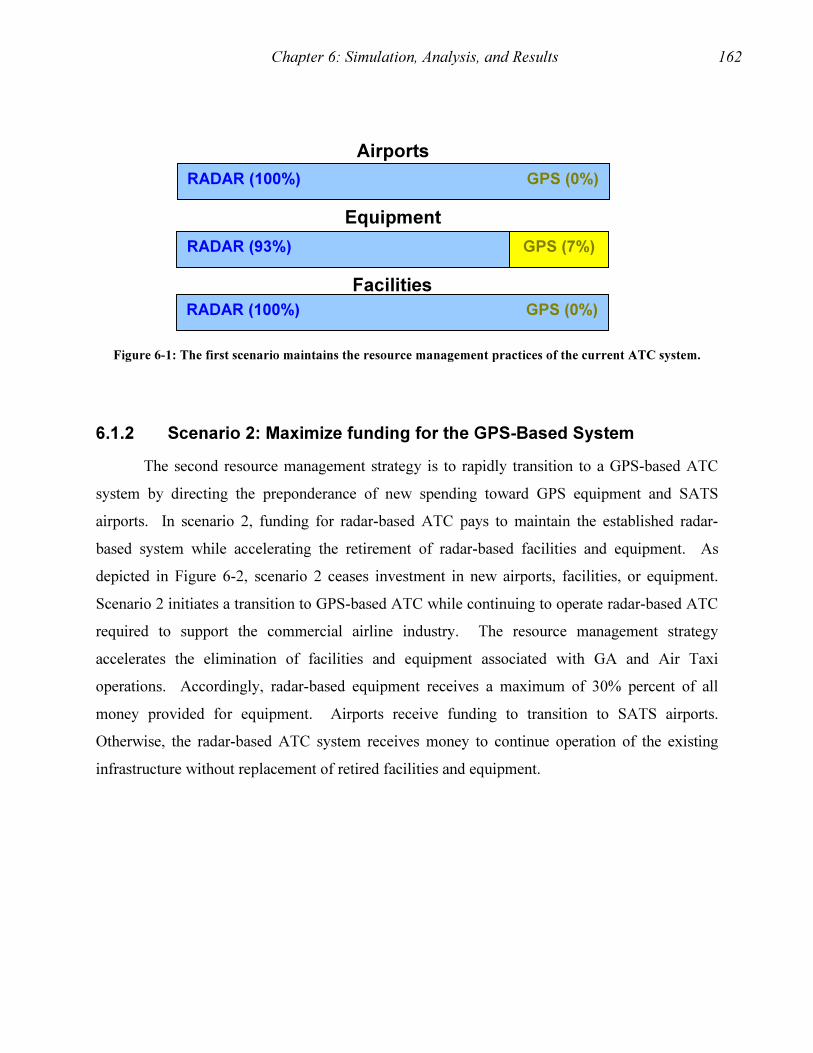
Chapter 6: Simulation, Analysis, and Results 162
Figure 6-1: The first scenario maintains the resource management practices of the current ATC system.
6.1.2 Scenario 2: Maximize funding for the GPS-Based System
The second resource management strategy is to rapidly transition to a GPS-based ATC
system by directing the preponderance of new spending toward GPS equipment and SATS
airports. In scenario 2, funding for radar-based ATC pays to maintain the established radar-
based system while accelerating the retirement of radar-based facilities and equipment. As
depicted in Figure 6-2, scenario 2 ceases investment in new airports, facilities, or equipment.
Scenario 2 initiates a transition to GPS-based ATC while continuing to operate radar-based ATC
required to support the commercial airline industry. The resource management strategy
accelerates the elimination of facilities and equipment associated with GA and Air Taxi
operations. Accordingly, radar-based equipment receives a maximum of 30% percent of all
money provided for equipment. Airports receive funding to transition to SATS airports.
Otherwise, the radar-based ATC system receives money to continue operation of the existing
infrastructure without replacement of retired facilities and equipment.
Airports
RADAR (93%) GPS (7%)
Equipment
RADAR (100%) GPS (0%)
Facilities
RADAR (100%) GPS (0%)

Chapter 6: Simulation, Analysis, and Results 163
Figure 6-2: The resource management strategy for the second scenario attempts to rapidly transition to GPS-
based ATC.
6.1.3 Scenario 3: Supplement the Radar-Based System
The third resource management strategy consists of a moderate transition to a combined
GPS- and radar-based ATC system. Funding for radar-based ATC pays to maintain the
established radar-based system and replace some of the retired radar-based facilities and
equipment. Simultaneously, the GPS-based ATC system expands through increased funding for
GPS-based equipment and acceleration of the transition of airports into SATS airports. Figure
6-3 depicts scenario 3 as a blend of both ATC capabilities.
Figure 6-3: The third scenario attempts to strike a balance between growth of GPS-based ATC and contiuity
of the radar-based system.
Airports
RADAR (30%) GPS (70%)
Equipment
RADAR (min) GPS (max)
Facilities
RADAR (min) GPS (max)
Airports
RADAR (75%) GPS (25%)
Equipment
RADAR (moderate) GPS (moderate)
Facilities
RADAR (moderate) GPS (moderate)

Chapter 6: Simulation, Analysis, and Results 164
6.2 Scenario 1: Simulation and Analysis of the Radar-based
System
The first scenario serves as a baseline for comparison to the other two scenarios. The first
scenario represents continuation of the FAA’s current means of controlling air traffic by using
radar-based facilities, equipment, and procedures. Although the resource management strategy
in Scenario 1 includes a small amount of funding for GPS-based ATC, resource managers
develop the FAA budget to maintain or expand the radar-based approach to ATC in the first
scenario. The simulation represents the 30-year time period from 1998 to 2028. The simulation
occurs over that time period because NASA planners anticipate it will be feasible to develop
SATS aircraft and establish a system of SATS airports and infrastructure by 2025 (NASA,
2000a).
6.2.1 Simulation of the Radar-based System
The simulation of the radar-based system demonstrated that the FAA will have sufficient
resources to support its mission to provide air traffic control, however, the Small Aircraft
Transportation System will not have sufficient resources to grow. Table 5-2 and Table 5-3 above
contain the initial stock and parameter values used in the base case. All the stocks are
endogenous to the system. The only exogenous variable, which is zero for scenario 1, is the
policy for the maximum percent of available funding resource managers should invest in the
GPS-based ATC system. Otherwise, all variables in the model are endogenous and reside in
feedback loops. The only major component of the model that is not endogenous is the Grants-in-
Aid account. The model contains a function to calculate the value of the Grants-in-Aid account
from a base year value and an annual growth rate that aligns with historical trends. Since the
first scenario represents continuity of the past FAA resource management strategy, managers do
not influence any of the variables any differently than they normally would.
The figures below contain output that describes the system’s behavior. The x-axis of
each graph represents the time period 1998 through 2028. The y-axis provides values for the
stocks in the model, parameters, or other metrics. The graphs depict the growth or decline of
system variables over time if the FAA continues to utilize a resource management strategy that
supports the radar-based approach to ATC. Figure 6-4 through Figure 6-6 describe the flow of
money through the major accounts of the budget. Figure 6-7 and Figure 6-8 show the flow of air

Chapter 6: Simulation, Analysis, and Results 165
traffic controllers and system maintainers. Figure 6-9 through Figure 6-14 depict the changes in
the Facilities and Equipment stocks. Figure 6-15 to Figure 6-18 illustrate the growth or decline
of the four aircraft stocks. Figure 6-19 and Figure 6-20 portray the adjustments in the growth or
decline of non-SATS or SATS airports.
Figure 6-4 depicts the general pattern of growth exhibited by the AATF under the first
scenario. Figure 6-5 shows an FAA budget growth pattern that aligns with the AATF growth.
Figure 6-6 shows the amount of funding the FAA requires from the General Fund to account for
the shortfalls in the AATF. Overall, the future flow of revenue and resources represents feasible
and acceptable conditions to enable the future operation of the ATC system.
Graph for Airport and Airways Trust Fund
40 B
30 B
20 B
10 B
0
1998 2000 2002 2004 2006 2008 2010 2012 2014 2016 2018 2020 2022 2024 2026 2028
Time (Year)
Airport and Airways Trust Fund : Base Dollars
Figure 6-4: Revenue generated by the Airport & Airways Trust Fund shows a general growth trend.

Chapter 6: Simulation, Analysis, and Results 166
Graph for FAA Budget
40 B
30 B
20 B
10 B
0
1998 2000 2002 2004 2006 2008 2010 2012 2014 2016 2018 2020 2022 2024 2026 2028
Time (Year)
FAA Budget : Base Dollars
Figure 6-5: Future FAA budgets will continue to grow.
Graph for general fund
6 B
4.5 B
3 B
1.5 B
0
1998 2000 2002 2004 2006 2008 2010 2012 2014 2016 2018 2020 2022 2024 2026 2028
Time (Year)
general fund : Base Dollars/Year
Figure 6-6: Congress supplements the FAA budget when there are AATF shortfalls.

Chapter 6: Simulation, Analysis, and Results 167
The following charts describe the behavior of three other parts of the ATC system: the
people, the facilities, and the equipment. Figure 6-7 depicts the changes in the numbers of Air
Traffic Controllers. There is decline of about 4,000 controllers during the first ten years of the
model, largely attributable to the retirement surge between 2003 and 2008. The system appears
to seek equilibrium of approximately 19,000 controllers. Figure 6-8 illustrates the changes in the
number of maintainers over time. Similar to the controllers, the maintainers undergo a long
steady decline in number due to retirements. Eventually, the training of new hires compensates
for the decline. The trend in facilities growth in Figure 6-9 through Figure 6-12 indicates
continued expansion of both Flight Service Stations and control towers. The FSSs portrayed in
Figure 6-9 primarily serve the non-commercial air traffic and the three types of control towers
depicted in Figure 6-10 to Figure 6-12 all serve a core portion of the aviation system. Under the
conditions of the first scenario, all three types of control towers show steady grow, with GA
towers being the most expansive. The radar-based equipment portrayed in Figure 6-13 neither
grows nor declines due to moderate system expansion offset by technological efficiencies. A
lack of resources constrains the growth of the stock of GPS equipment in Figure 6-14.
Graph for Controllers
40,000
32,500
25,000
17,500
10,000
1998 2000 2002 2004 2006 2008 2010 2012 2014 2016 2018 2020 2022 2024 2026 2028
Time (Year)
Controllers : Base People
Figure 6-7: Retirements cause an initial decline in the controller population.

Chapter 6: Simulation, Analysis, and Results 168
Graph for Maintainers
10,000
9,000
8,000
7,000
6,000
1998 2000 2002 2004 2006 2008 2010 2012 2014 2016 2018 2020 2022 2024 2026 2028
Time (Year)
Maintainers : Base People
Figure 6-8: The maintainer-training program eventually compensates for retirements.
Graph for FSSs
200
175
150
125
100
1998 2000 2002 2004 2006 2008 2010 2012 2014 2016 2018 2020 2022 2024 2026 2028
Time (Year)
FSSs : Base FSSs
Figure 6-9: Flight Service Stations continue a steady climb in number.
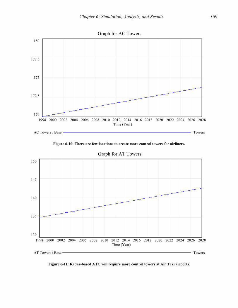
Chapter 6: Simulation, Analysis, and Results 169
Graph for AC Towers
180
177.5
175
172.5
170
1998 2000 2002 2004 2006 2008 2010 2012 2014 2016 2018 2020 2022 2024 2026 2028
Time (Year)
AC Towers : Base Towers
Figure 6-10: There are few locations to create more control towers for airliners.
Graph for AT Towers
150
145
140
135
130
1998 2000 2002 2004 2006 2008 2010 2012 2014 2016 2018 2020 2022 2024 2026 2028
Time (Year)
AT Towers : Base Towers
Figure 6-11: Radar-based ATC will require more control towers at Air Taxi airports.

Chapter 6: Simulation, Analysis, and Results 170
Graph for GA Towers
200
175
150
125
100
1998 2000 2002 2004 2006 2008 2010 2012 2014 2016 2018 2020 2022 2024 2026 2028
Time (Year)
GA Towers : Base Towers
Figure 6-12: General Aviation control towers will continue to grow in numbers.
Graph for Radar based Equipment
8,000
7,500
7,000
6,500
6,000
1998 2000 2002 2004 2006 2008 2010 2012 2014 2016 2018 2020 2022 2024 2026 2028
Time (Year)
Radar based Equipment : Base Eqpt
Figure 6-13: The pool of radar-based equipment remains constant in the first scenario.

Chapter 6: Simulation, Analysis, and Results 171
Graph for GPS based Equipment
400
300
200
100
0
1998 2000 2002 2004 2006 2008 2010 2012 2014 2016 2018 2020 2022 2024 2026 2028
Time (Year)
GPS based Equipment : Base Eqpt
Figure 6-14: The GPS-based equipment decommission rate eventually overtakes the installation rate.
The model addresses two other key parts of the ATC system: aircraft and airports. Figure
6-15 to Figure 6-18 describe the populations of AC, AT, GA, and SATS aircraft. The AC
aircraft in Figure 6-15 plateau in number around 2010 due to inherent limitations in the ATC
system. The timeframe and behavior of the AC population also corresponds with the NASA
study discussed previously in section 2.1 and depicted in Figure 2-3. The AT and GA aircraft
show continued growth in Figure 6-16 and Figure 6-17, unconstrained by the more restrictive
limitations of the ATC system placed on the AC aircraft. The number of SATS aircraft, depicted
in Figure 6-18, does not grow beyond a minor experimental fleet in the first scenario, due to a
lack of supporting GPS infrastructure.
Figure 6-19 and Figure 6-20 capture the changes in the population of SATS and non-
SATS airports. The non-SATS airports in Figure 6-19 continue to decline in number due to the
normal demise of public use airports at the rate of approximately one every two weeks. The
growth in SATS airports in Figure 6-20 during the first scenario results from a modest
conversion rate of one public use airport into a new airport every two years to support the
experimental fleet of SATS aircraft.
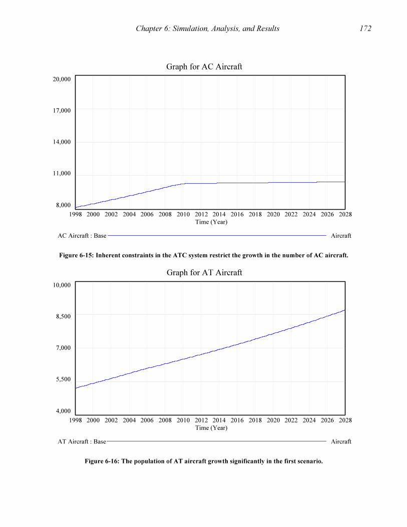
Chapter 6: Simulation, Analysis, and Results 172
Graph for AC Aircraft
20,000
17,000
14,000
11,000
8,000
1998 2000 2002 2004 2006 2008 2010 2012 2014 2016 2018 2020 2022 2024 2026 2028
Time (Year)
AC Aircraft : Base Aircraft
Figure 6-15: Inherent constraints in the ATC system restrict the growth in the number of AC aircraft.
Graph for AT Aircraft
10,000
8,500
7,000
5,500
4,000
1998 2000 2002 2004 2006 2008 2010 2012 2014 2016 2018 2020 2022 2024 2026 2028
Time (Year)
AT Aircraft : Base Aircraft
Figure 6-16: The population of AT aircraft growth significantly in the first scenario.

Chapter 6: Simulation, Analysis, and Results 173
Graph for GA Aircraft
80,000
75,000
70,000
65,000
60,000
1998 2000 2002 2004 2006 2008 2010 2012 2014 2016 2018 2020 2022 2024 2026 2028
Time (Year)
GA Aircraft : Base Aircraft
Figure 6-17: The number of GA aircraft grows continuously in a radar-based ATC system.
Graph for SATS Aircraft
40
30
20
10
0
1998 2000 2002 2004 2006 2008 2010 2012 2014 2016 2018 2020 2022 2024 2026 2028
Time (Year)
SATS Aircraft : Base Aircraft
Figure 6-18: The lack of GPS support precludes the growth of the SATS program.
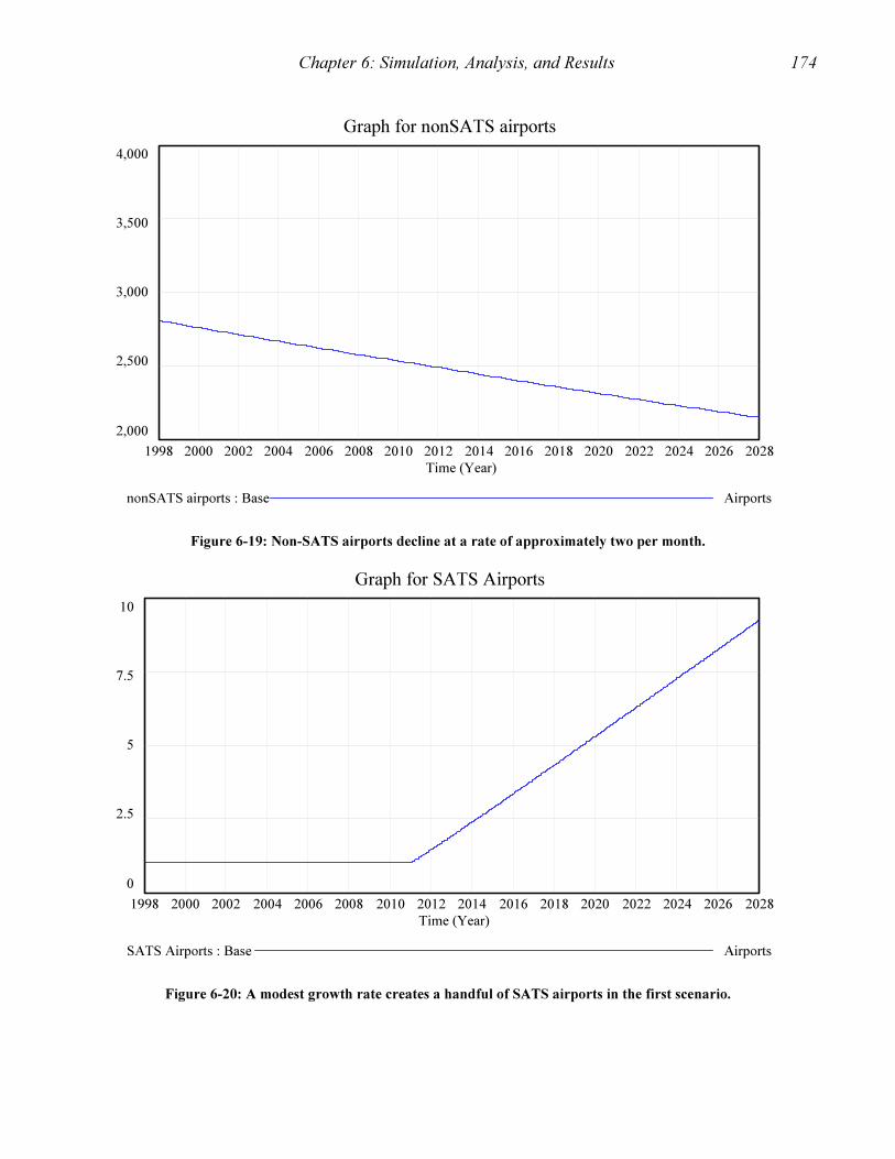
Chapter 6: Simulation, Analysis, and Results 174
Graph for nonSATS airports
4,000
3,500
3,000
2,500
2,000
1998 2000 2002 2004 2006 2008 2010 2012 2014 2016 2018 2020 2022 2024 2026 2028
Time (Year)
nonSATS airports : Base Airports
Figure 6-19: Non-SATS airports decline at a rate of approximately two per month.
Graph for SATS Airports
10
7.5
5
2.5
0
1998 2000 2002 2004 2006 2008 2010 2012 2014 2016 2018 2020 2022 2024 2026 2028
Time (Year)
SATS Airports : Base Airports
Figure 6-20: A modest growth rate creates a handful of SATS airports in the first scenario.

Chapter 6: Simulation, Analysis, and Results 175
6.2.2 Analysis of Scenario 1
The results of the ATC Resource Management Model for the first scenario showed that
the ATC system will continue to function almost as it has for the past decade. Nevertheless,
there are several exceptions to the normal behavior patterns: GPS equipment enters the system
and slowly fades away, AC aircraft growth plateaus, radar-based equipment plateaus, and a
modest amount of SATS aircraft and SATS airports enter the ATC system. However, the SATS
does not establish itself and survive as a transportation system. Despite the exceptions to normal
behavior, the first scenario includes two components that allow it to serve as a good baseline.
First, the scenario includes a viable radar-based ATC system, and second, the scenario will not
support the growth of the SATS.
Several characteristics of the system indicate that it will continue to operate as viably as it
had in the past. First, the flow of dollar resources provides adequate revenue to the AATF,
which in turn supports the requirements emanating from the FAA budget. Table 6-1 shows that
the requirements of the FAA budget continue to generally align with those of the past. Some of
the funding appears to migrate from the Facilities and Equipment account to the Grants-in-Aid
account. Second, Figure 6-21 shows how the growth in facilities, in this case control towers,
also reflects past growth trends. However, the model growth is less aggressive than the actual
growth exhibited in the 1990s. The decline in growth rate makes sense in light of the plateau of
AC aircraft, which may indicate a reduction in overall system growth. Third, the ratio of the
number of AT and GA aircraft per airport (IFR capable aircraft per the pool of 2,400 Public Use
airports), which varied between 20 and 30 IFR aircraft per airport in the 1980s and 1990s, grew
steadily into the upper 30s in the model as illustrated in Figure 6-22. However, the decline in the
number of available airports depicted in Figure 6-19 above explains why the aircraft to airports
ratio grew so much.
Table 6-1: The distribution of resources among the major accounts of the FAA budget changes slightly.
Account 2000 2004 2008 2012 2016 2020 2024 2028 1991 – 2002
Grants 19% 25% 28% 27% 28% 29% 29% 29% 22%
Ops 60% 54% 52% 54% 54% 55% 55% 56% 54%
F&E 20% 21% 21% 19% 18% 17% 16% 15% 23%

Chapter 6: Simulation, Analysis, and Results 176
380
400
420
440
460
480
500
520
1992 1996 2000 2004 2008 2012 2016 2020 2024 2028
Year
# o
f T
ow
ers
Model
Actual
Figure 6-21: The Control Tower growth rate declines from that of the 1990s.
Graph for nonSATS acft per nonSATS airports
40
35
30
25
20
1998 2000 2002 2004 2006 2008 2010 2012 2014 2016 2018 2020 2022 2024 2026 2028
Time (Year)
nonSATS acft per nonSATS airports : Base Aircraft/Airports
Figure 6-22: The decline in public use airports attributed to the growth in the aircraft/airports ratio.

Chapter 6: Simulation, Analysis, and Results 177
The characteristics of the ATC system that differ in the future will not preclude the system
from functioning. Despite the plateau in the number of AC aircraft beginning in 2010, the AATF
and FAA budgets differ by an acceptable amount. The US Congress appropriates funds from the
US General Fund, depicted in Figure 6-6 above, to account for the differences between the
AATF and the FAA budget. The US Congress established the AATF in 1970s to create a source
of funds for the Facilities and Equipment account and the Grants-in-Aid account, as well as at
least 36% of the annual FAA operations account, which means the General Fund contribution
must be 20 % or less. Thus the shortfall covered by the General Fund, recorded in Table 6-2,
complies with the Congressional requirement.
Table 6-2: Over time, the percentage amount of funding provided by Congress for the FAA budget increases.
Account $M 2000 2004 2008 2012 2016 2020 2024 2028
Gen Fund $0 0.623 1,436 1,688 1,966 2,796 3,826 4,982
FAA Budget 9,419 12,320 13,840 16,160 18,410 20,500 22,750 25,150
Gen Fund % 0.00% 0.01% 10% 11% 11% 14% 17% 20%
The plateau in radar-based equipment in Figure 6-13 reflects technological efficiencies
that reduce the number of equipment needed in the system. Additionally, the technological
capabilities of aircraft will allow them to conduct many radar-based navigation tasks by using
GPS receivers that do not require GPS-based ATC equipment on the ground.
Conversely, SATS requires the precision and signal assurance of the ground-based GPS
augmentation systems to enable safe landings, aircraft separation, moving map displays, and
ground operations. Figure 6-14 above shows the decline of GPS-based equipment in the first
scenario. The loss of GPS equipment combined with the small amount of SATS airports
depicted in Figure 6-20, caused a lack of SATS infrastructure. The lack of SATS infrastructure
in the first scenario prohibited the system from advancing beyond a small number of
experimental aircraft and airports. The source of airports and aircraft came from intentional
construction rather than system driven conversion of non-SATS aircraft and airports. From a
performance metrics standpoint, the first scenario stacks up as follows: the AATF is sufficient to
maintain a viable ATC system, but the number of SATS aircraft, SATS airports, and ground-
based GPS equipment precludes the establishment of the Small Aircraft Transportation System.

Chapter 6: Simulation, Analysis, and Results 178
6.3 Scenario 2: Simulation and Analysis of the GPS-based
System The second scenario represents a major change in the philosophy of ATC within the FAA.
In this scenario, resources managers shift resources away from the radar-based approach to the
GPS-based approach for the AT and GA communities. The second scenario maintains the radar-
based system as the primary means of ATC for commercial AC airliners. However, those
airports, facilities, and equipment outside of the hub and spoke system undergo a 5-year
transition to GPS-based ATC from 2005 until 2010. During that time period, resource managers
direct funding away from the radar-based facilities and equipment that support AT and GA
aircraft. The resources support the installation and maintenance of GPS-based equipment and
the conversion of airports into SATS airports. As in the first scenario, the simulation represents
the 30-year time period from 1998 to 2028.
6.3.1 Simulation of the GPS-based System
The simulation of the GPS-based system demonstrated that the FAA will have sufficient
resources to support its mission to provide air traffic control, the Small Aircraft Transportation
System will have sufficient resources to grow, however, there is a disturbing decline in radar-
based equipment that may induce safety or delay problems not captured by the model.
Additionally, feedback from the changes in the system causes the population of AC aircraft to
decline beginning in about 2010. As in the base case, Table 5-2 and Table 5-3 above contain the
initial stock and parameter values used in the second scenario as well. All the stocks are
endogenous to the system. The only exogenous variable, which is 100% for scenario 2, is the
policy for the maximum percent of available funding resource managers should invest in the
GPS-based ATC system. The resource managers linearly increase the transfer of funding from
the radar-based approach to the GPS-based approach over the five-year period. Otherwise, all
variables in the model are endogenous and reside in feedback loops. As explained in scenario 1
above, the only major component of the model that is not endogenous is the Grants-in-Aid
account. The second scenario represents a radical change from past FAA resource management
strategies; managers purposefully underfund the radar-based approach to ATC in order to
advance the GPS-based approach, which is necessary for the success of the SATS.
The figures below contain the same series of output that describes the system’s behavior
under the conditions of both the first scenario in blue, and the second scenario in red. Again, the

Chapter 6: Simulation, Analysis, and Results 179
x-axis of each graph represents the time period 1998 through 2028 and the y-axis provides values
for the stocks, parameters, or other metrics. The lines in blue depict the growth or decline of
system variables over time from the first scenario. The lines in red depict the changes in system
variables if the FAA changes to a resource management strategy that supports the GPS-based
approach to ATC. Figure 6-23 through Figure 6-25 describe the flow of money through the
major accounts of the budget. Figure 6-26 and Figure 6-27 show the flow of air traffic
controllers and system maintainers. Figure 6-28 through Figure 6-33 depict the changes in the
Facilities and Equipment stocks. Figure 6-34 to Figure 6-37 illustrate the growth or decline of
the four aircraft stocks. Figure 6-38 and Figure 6-39 portray the adjustments in the growth or
decline of non-SATS or SATS airports.
Figure 6-23 depicts the general pattern of growth exhibited by the AATF under the first
and second scenarios. Figure 6-24 shows that the FAA budget growth pattern of the second
scenario aligns closely with the budget from the first scenario. The budgets are similar because
the reductions in some parts of the infrastructure, such as control towers, are offset by increases
in other parts of the system, such as Flight Service Stations. Figure 6-25 shows that the amount
of funding the FAA requires from the General Fund under the second scenario increase from the
amount required in the first scenario to account for the shortfalls in the AATF. Congress may
not support the increase in funding from the General Fund required under the second scenario.
Thus, the future flow of revenue and resources may place the feasibility and acceptability of the
second scenario in jeopardy.
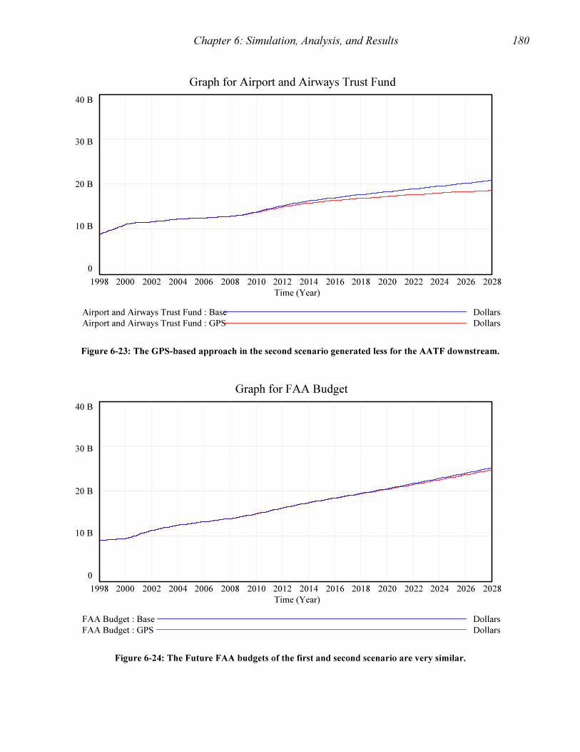
Chapter 6: Simulation, Analysis, and Results 180
Graph for Airport and Airways Trust Fund
40 B
30 B
20 B
10 B
0
1998 2000 2002 2004 2006 2008 2010 2012 2014 2016 2018 2020 2022 2024 2026 2028
Time (Year)
Airport and Airways Trust Fund : Base Dollars
Airport and Airways Trust Fund : GPS Dollars
Figure 6-23: The GPS-based approach in the second scenario generated less for the AATF downstream.
Graph for FAA Budget
40 B
30 B
20 B
10 B
0
1998 2000 2002 2004 2006 2008 2010 2012 2014 2016 2018 2020 2022 2024 2026 2028
Time (Year)
FAA Budget : Base Dollars
FAA Budget : GPS Dollars
Figure 6-24: The Future FAA budgets of the first and second scenario are very similar.

Chapter 6: Simulation, Analysis, and Results 181
Graph for general fund
8 B
6 B
4 B
2 B
0
1998 2000 2002 2004 2006 2008 2010 2012 2014 2016 2018 2020 2022 2024 2026 2028
Time (Year)
general fund : Base Dollars/Year
general fund : GPS Dollars/Year
Figure 6-25: The additional funding required by the second scenario may jeopardize its implementation.
The following charts describe the behavior of three other parts of the ATC system: the
people, the facilities, and the equipment. Figure 6-26 shows that the GPS-based ATC system
will not reduce the need for air traffic controllers for two reasons. First, the demands of the hub
and spoke system require controllers in the facilities remaining in the system. Secondly,
controllers who work in the facilities that do close will migrate to the expanded population of
Flight Service Stations. Figure 6-27 illustrates the changes in the number of maintainers over
time. Two factors account for the behavior of the maintainer stock over time. First, accelerated
retirements due to an aged population causes the downward slope beginning in 2010. Second,
the decline in radar-based ATC equipment, depicted in Figure 6-32, causes a large reduction in
the need for maintainers after 2012 despite the increase in GPS-based equipment in Figure 6-33.
The trend in facilities growth in Figure 6-28 through Figure 6-31 indicates an even
greater expansion of Flight Service Stations in the second scenario, but a reduction in the growth
of control towers. The FSSs portrayed in Figure 6-28 continue to serve the non-commercial air
traffic and the expanding fleet of SATS aircraft. Each of the three types of control towers
depicted in Figure 6-29 to Figure 6-31 face decline in their numbers. The GA Towers face the

Chapter 6: Simulation, Analysis, and Results 182
greatest decline as the SATS aircraft fill in for the loss of the GA portion of the aviation system.
The radar-based ATC equipment depicted in Figure 6-32 undergoes significant reductions due to
the resource management strategy that emphasizes GPS equipment. Conversely, Figure 6-33
shows the increase in ground-based GPS equipment that enables the GPS-based approach to
ATC.
Graph for Controllers
40,000
32,500
25,000
17,500
10,000
1998 2000 2002 2004 2006 2008 2010 2012 2014 2016 2018 2020 2022 2024 2026 2028
Time (Year)
Controllers : Base People
Controllers : GPS People
Figure 6-26: The GPS-based approach to ATC requires controllers to enable the Hub and Spoke system.

Chapter 6: Simulation, Analysis, and Results 183
Graph for Maintainers
10,000
9,000
8,000
7,000
6,000
1998 2000 2002 2004 2006 2008 2010 2012 2014 2016 2018 2020 2022 2024 2026 2028
Time (Year)
Maintainers : Base People
Maintainers : GPS People
Figure 6-27: The reduction in radar-based equipment reduces the need for maintainers after 2012.
Graph for FSSs
400
325
250
175
100
1998 2000 2002 2004 2006 2008 2010 2012 2014 2016 2018 2020 2022 2024 2026 2028
Time (Year)
FSSs : Base FSSs
FSSs : GPS FSSs
Figure 6-28: Flight Service Stations continue to serve a larger audience due to the expansion of SATS.

Chapter 6: Simulation, Analysis, and Results 184
Graph for AC Towers
180
175
170
165
160
1998 2000 2002 2004 2006 2008 2010 2012 2014 2016 2018 2020 2022 2024 2026 2028
Time (Year)
AC Towers : Base Towers
AC Towers : GPS Towers
Figure 6-29: The change in resource management causes a reduction in the population of AC towers.
Graph for AT Towers
200
175
150
125
100
1998 2000 2002 2004 2006 2008 2010 2012 2014 2016 2018 2020 2022 2024 2026 2028
Time (Year)
AT Towers : Base Towers
AT Towers : GPS Towers
Figure 6-30: An emphasis on GPS-based ATC will reduce the requirement for control towers at AT airports.

Chapter 6: Simulation, Analysis, and Results 185
Graph for GA Towers
200
175
150
125
100
1998 2000 2002 2004 2006 2008 2010 2012 2014 2016 2018 2020 2022 2024 2026 2028
Time (Year)
GA Towers : Base Towers
GA Towers : GPS Towers
Figure 6-31: General Aviation control towers decline under the second scenario.
Graph for Radar based Equipment
8,000
6,000
4,000
2,000
0
1998 2000 2002 2004 2006 2008 2010 2012 2014 2016 2018 2020 2022 2024 2026 2028
Time (Year)
Radar based Equipment : Base Eqpt
Radar based Equipment : GPS Eqpt
Figure 6-32: The change in resource management causes a decline in the pool of radar-based equipment.

Chapter 6: Simulation, Analysis, and Results 186
Graph for GPS based Equipment
1,000
750
500
250
0
1998 2000 2002 2004 2006 2008 2010 2012 2014 2016 2018 2020 2022 2024 2026 2028
Time (Year)
GPS based Equipment : Base Eqpt
GPS based Equipment : GPS Eqpt
Figure 6-33: The GPS-based equipment pool expands under the second scenario.
The model addresses two other key parts of the ATC system: aircraft and airports. Figure
6-34 to Figure 6-37 describe the populations of AC, AT, GA, and SATS aircraft. The growth of
AC aircraft in Figure 6-34 peaks around 2010 as a result of the reduction in capabilities of the
radar-based ATC system caused by the resource management strategy used in the second
scenario. The reduction in the AC population after 2010 is a significant negative effect of the
second scenario that may make the resource management approach unacceptable to policy
makers. Large declinations in the population of AT and GA aircraft also begin after
approximately 2010 as depicted in Figure 6-35 and Figure 6-36. The number of SATS aircraft,
depicted in Figure 6-37, grows rapidly due to conversions of AT and GA aircraft into SATS
aircraft, enabled by the growth of supporting GPS infrastructure in the second scenario.
Figure 6-38 and Figure 6-39 capture the changes in the population of SATS and non-
SATS airports. The non-SATS airports in Figure 6-38 continue to decline in number due to the
normal demise of public use airports. However, many of the airports converted from non-SATS
airports into SATS airports. The growth in SATS airports in Figure 6-39 during the second
scenario enabled the establishment of the SATS as a viable transportation system.

Chapter 6: Simulation, Analysis, and Results 187
Graph for AC Aircraft
20,000
17,000
14,000
11,000
8,000
1998 2000 2002 2004 2006 2008 2010 2012 2014 2016 2018 2020 2022 2024 2026 2028
Time (Year)
AC Aircraft : Base Aircraft
AC Aircraft : GPS Aircraft
Figure 6-34: Feedback from the GPS-based system further restrains the growth in the number of AC aircraft.
Graph for AT Aircraft
10,000
7,500
5,000
2,500
0
1998 2000 2002 2004 2006 2008 2010 2012 2014 2016 2018 2020 2022 2024 2026 2028
Time (Year)
AT Aircraft : Base Aircraft
AT Aircraft : GPS Aircraft
Figure 6-35: The population of AT aircraft growth declines with the onset of SATS.
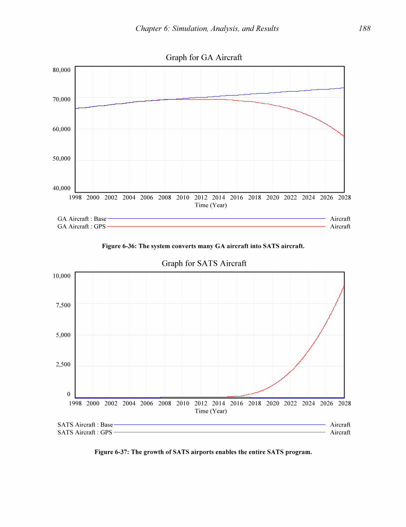
Chapter 6: Simulation, Analysis, and Results 188
Graph for GA Aircraft
80,000
70,000
60,000
50,000
40,000
1998 2000 2002 2004 2006 2008 2010 2012 2014 2016 2018 2020 2022 2024 2026 2028
Time (Year)
GA Aircraft : Base Aircraft
GA Aircraft : GPS Aircraft
Figure 6-36: The system converts many GA aircraft into SATS aircraft.
Graph for SATS Aircraft
10,000
7,500
5,000
2,500
0
1998 2000 2002 2004 2006 2008 2010 2012 2014 2016 2018 2020 2022 2024 2026 2028
Time (Year)
SATS Aircraft : Base Aircraft
SATS Aircraft : GPS Aircraft
Figure 6-37: The growth of SATS airports enables the entire SATS program.

Chapter 6: Simulation, Analysis, and Results 189
Graph for nonSATS airports
4,000
3,250
2,500
1,750
1,000
1998 2000 2002 2004 2006 2008 2010 2012 2014 2016 2018 2020 2022 2024 2026 2028
Time (Year)
nonSATS airports : Base Airports
nonSATS airports : GPS Airports
Figure 6-38: Non-SATS airports decline at a rate of approximately two per month.
Graph for SATS Airports
400
300
200
100
0
1998 2000 2002 2004 2006 2008 2010 2012 2014 2016 2018 2020 2022 2024 2026 2028
Time (Year)
SATS Airports : Base Airports
SATS Airports : GPS Airports
Figure 6-39: The growth of SATS airports enables the entire SATS program.

Chapter 6: Simulation, Analysis, and Results 190
6.3.2 Analysis of Scenario 2
The data generated from the second scenario indicates that the resource management
strategy favoring GPS may be both unacceptable and infeasible. The second scenario is
unacceptable to Congress because it eventually necessitates high expenditures of General Funds
beyond the limits set by Congress. Table 6-3 contains the percentages of General Funds required
by the second scenario. Congress will not accept requirements to transfer more than 20% of the
FAA budget from the General Fund. The second scenario is infeasible because it creates a
reduction in the populations of AC aircraft and radar-based ATC equipment. The reduction of
AC aircraft reduces the capacity of the aviation system to serve the nation. The reduction of the
number of radar-based equipment increases the likelihood that there will be accidents or delays
in the NAS. Therefore, the second scenario represents an infeasible option because of the
potential for delay, AC capacity reduction, and a decline in safety. The lack of radar-based ATC
equipment serves as a surrogate measure of delay and safety.
Table 6-3: Congress will refrain from funding more than 20% of the FAA budget from the General Fund.
Account $M 2000 2004 2008 2012 2016 2020 2024 2028
Gen Fund $0 0.623 1,441 1,985 2,541 3,639 5,030 6,744
FAA Budget 9,419 12,320 13,840 16,160 18,410 20,500 22,750 25,150
Gen Fund % 0.00% 0.01% 10% 12% 14% 18% 22% 27%
Despite the infeasibility and unacceptability of the second scenario, it shows that the
system has the potential to generate revenue and create the conditions for the growth and
maturation of the SATS. Figure 6-40 shows the conversion of public use airports into SATS
airports. Without conversion to SATS, the airports would no longer contribute to the NAS.
Similarly, Figure 6-41 shows the conversion of AT and GA aircraft into SATS aircraft. In both
cases, the SATS consists of a modest proportion of the entire system. Although the ATC
resource management devoting the maximum resources towards the GPS-based approach proved
infeasible and unacceptable in the second scenario, the establishment of SATS in the second
scenario indicates that a compromise solution may support SATS and provide adequate revenue
for the ATC system. The third scenario in the next section represents a less extreme departure
from the normal conservative culture of the FAA, which consists using GPS-based ATC to
supplement the radar-based ATC system.

Chapter 6: Simulation, Analysis, and Results 191
0
500
1000
1500
2000
2500
3000
2000 2004 2008 2012 2016 2020 2024 2028
Year
# o
f A
irp
ort
s
SATS
NonSATS
Figure 6-40: The conversion of non-SATS airports into SATS airports begins in approximately 2012.
0
10000
20000
30000
40000
50000
60000
70000
80000
2000 2004 2008 2012 2016 2020 2024 2028
Year
# o
f A
irp
ort
s
SATS
GA
AT
Figure 6-41: Many AT and some GA aircraft convert into SATS aircraft.

Chapter 6: Simulation, Analysis, and Results 192
6.4 Scenario 3: Simulation and Analysis of the radar-based
system supplemented by GPS
The third scenario represents a moderate change in the philosophy of ATC within the FAA
that is more in keeping with the conservative culture of the organization. In this scenario,
resources managers shift 25% of the resources away from the radar-based approach to the GPS-
based approach to ATC. The resource shift occurs over a ten-year period from 2015 to 2025.
From 2025 and beyond, the FAA continues to support the GPS-based approach to ATC with
25% of the funding that normally would have gone to continuation of the radar-based system.
The resources support the radar-based system and also support installation and maintenance of
GPS-based equipment and the conversion of airports into SATS airports. As in the previous
scenarios, the simulation represents the 30-year time period from 1998 to 2028.
6.4.1 Simulation of the radar-based system supplemented by GPS
The simulation of the radar-based system supplemented by GPS demonstrated that the
FAA will generally have sufficient resources to support its mission to provide air traffic control,
and, the Small Aircraft Transportation System will have sufficient resources to grow at a modest
rate. The third scenario represents a conservative compromise that places slight risk on future
FAA revenue, but gives the SATS a chance to become established as a viable transportation
system. As in the previous cases, Table 5-2 and Table 5-3 above contain the initial stock and
parameter values used in the second scenario as well. All the stocks are endogenous to the
system. The only exogenous variable, which is 25% for scenario 3, is the policy for the
maximum percent of available funding resource managers should invest in the GPS-based ATC
system. The resource managers linearly increase the transfer of funding from the radar-based
approach to the GPS-based approach over the ten-year period from 2015 to 2025. Otherwise, all
variables in the model are endogenous and reside in feedback loops. As explained in the
previous scenarios above, the only major component of the model that is not endogenous is the
Grants-in-Aid account. The third scenario represents a moderate change from past FAA resource
management strategies; managers attempt to balance the radar-based approach to ATC with

Chapter 6: Simulation, Analysis, and Results 193
supplemental support from the GPS-based approach, which is necessary for the success of the
SATS.
The figures below contain the same series of output used in the first two scenarios to
describe the system’s behavior. The first scenario is in blue, the second scenario in red, and the
third scenario in green. In many cases the blue and green lines overlap. Again, the x-axis of
each graph represents the time period 1998 through 2028 and the y-axis provides values for the
stocks, parameters, or other metrics. The colored lines depict the growth or decline of system
variables over time. Figure 6-42 through Figure 6-44 describe the flow of money through the
major accounts of the budget. Figure 6-45 and Figure 6-46 show the flow of air traffic
controllers and system maintainers. Figure 6-47 through Figure 6-52 depict the changes in the
Facilities and Equipment stocks. Figure 6-53 to Figure 6-56 illustrate the growth or decline of
the four aircraft stocks. Figure 6-57 and Figure 6-58 portray the adjustments in the growth or
decline of non-SATS or SATS airports.
Figure 6-42 depicts the general pattern of growth exhibited by the AATF under the three
scenarios. The third scenario aligns closely with the first. Figure 6-43 shows that the FAA
budget growth pattern of the third scenario is almost identical to the budget from the first
scenario. The budgets are similar because the delayed introduction of GPS funding until 2015
and the slow transition to the 25% funding level caused little change in the FAA budget. Figure
6-44 shows that the amount of funding the FAA required from the General Fund under the third
scenario increased just slightly from the amount required in the first scenario to account for the
shortfalls in the AATF. Congress will support the minimal increase in funding from the General
Fund required under the second scenario. Thus, the future flow of revenue and resources makes
the third scenario economically feasible.

Chapter 6: Simulation, Analysis, and Results 194
Graph for Airport and Airways Trust Fund
40 B
30 B
20 B
10 B
0
1998 2000 2002 2004 2006 2008 2010 2012 2014 2016 2018 2020 2022 2024 2026 2028
Time (Year)
Airport and Airways Trust Fund : Base Dollars
Airport and Airways Trust Fund : GPS Dollars
Airport and Airways Trust Fund : Mix Dollars
Figure 6-42: The third scenario aligns closely with the first.
Graph for FAA Budget
40 B
30 B
20 B
10 B
0
1998 2000 2002 2004 2006 2008 2010 2012 2014 2016 2018 2020 2022 2024 2026 2028
Time (Year)
FAA Budget : Base Dollars
FAA Budget : GPS Dollars
FAA Budget : Mix Dollars
Figure 6-43: The Future FAA budgets of the first and third scenario are almost identical.

Chapter 6: Simulation, Analysis, and Results 195
Graph for general fund
8 B
6 B
4 B
2 B
0
1998 2000 2002 2004 2006 2008 2010 2012 2014 2016 2018 2020 2022 2024 2026 2028
Time (Year)
general fund : Base Dollars/Year
general fund : GPS Dollars/Year
general fund : Mix Dollars/Year
Figure 6-44: The minimal additional funding required by the third scenario makes it feasible.
The following charts describe the behavior of three other parts of the ATC system: the
people, the facilities, and the equipment. Figure 6-45 shows that the radar-based and GPS-
supplemented ATC system will not reduce the need for air traffic controllers. Figure 6-46
illustrates the changes in the number of maintainers over time caused primarily by retirements.
The trend in facilities growth in Figure 6-47 through Figure 6-50 indicates an even greater
expansion of Flight Service Stations in the second scenario, but a reduction in the growth of
control towers. The FSSs portrayed in Figure 6-47 continue to serve the non-commercial air
traffic and the expanding fleet of SATS aircraft. Each of the three types of control towers
depicted in Figure 6-48 to Figure 6-50 face decline in their numbers. The GA Towers face the
greatest decline as the SATS aircraft fill in for the loss of the GA portion of the aviation system.
The radar-based ATC equipment depicted in Figure 6-51 undergoes significant reductions due to
the resource management strategy that emphasizes GPS equipment. Conversely, Figure 6-52
shows the increase in ground-based GPS equipment that enables the GPS-based approach to
ATC.
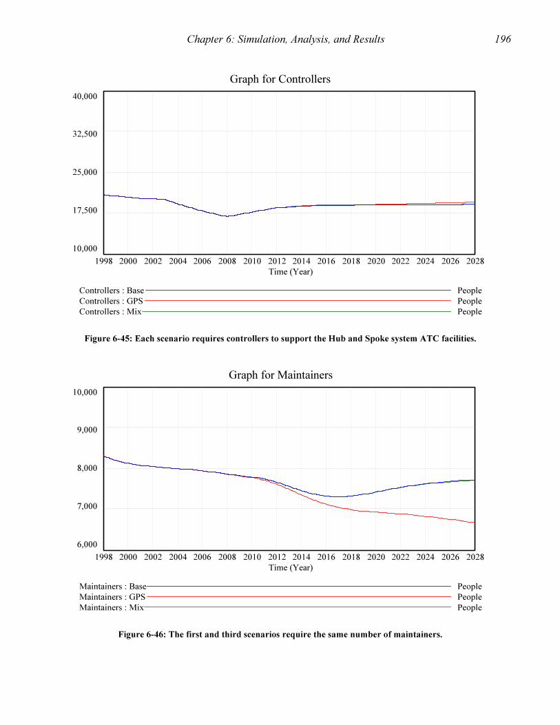
Chapter 6: Simulation, Analysis, and Results 196
Graph for Controllers
40,000
32,500
25,000
17,500
10,000
1998 2000 2002 2004 2006 2008 2010 2012 2014 2016 2018 2020 2022 2024 2026 2028
Time (Year)
Controllers : Base People
Controllers : GPS People
Controllers : Mix People
Figure 6-45: Each scenario requires controllers to support the Hub and Spoke system ATC facilities.
Graph for Maintainers
10,000
9,000
8,000
7,000
6,000
1998 2000 2002 2004 2006 2008 2010 2012 2014 2016 2018 2020 2022 2024 2026 2028
Time (Year)
Maintainers : Base People
Maintainers : GPS People
Maintainers : Mix People
Figure 6-46: The first and third scenarios require the same number of maintainers.

Chapter 6: Simulation, Analysis, and Results 197
Graph for FSSs
400
325
250
175
100
1998 2000 2002 2004 2006 2008 2010 2012 2014 2016 2018 2020 2022 2024 2026 2028
Time (Year)
FSSs : Base FSSs
FSSs : GPS FSSs
FSSs : Mix FSSs
Figure 6-47: There is a slight growth in the number of Flight Service Stations in the third scenario.
Graph for AC Towers
180
175
170
165
160
1998 2000 2002 2004 2006 2008 2010 2012 2014 2016 2018 2020 2022 2024 2026 2028
Time (Year)
AC Towers : Base Towers
AC Towers : GPS Towers
AC Towers : Mix Towers
Figure 6-48: The third scenario causes a slight reduction in the population of AC towers.
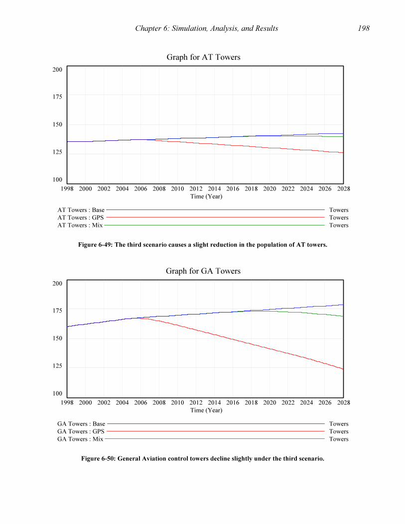
Chapter 6: Simulation, Analysis, and Results 198
Graph for AT Towers
200
175
150
125
100
1998 2000 2002 2004 2006 2008 2010 2012 2014 2016 2018 2020 2022 2024 2026 2028
Time (Year)
AT Towers : Base Towers
AT Towers : GPS Towers
AT Towers : Mix Towers
Figure 6-49: The third scenario causes a slight reduction in the population of AT towers.
Graph for GA Towers
200
175
150
125
100
1998 2000 2002 2004 2006 2008 2010 2012 2014 2016 2018 2020 2022 2024 2026 2028
Time (Year)
GA Towers : Base Towers
GA Towers : GPS Towers
GA Towers : Mix Towers
Figure 6-50: General Aviation control towers decline slightly under the third scenario.
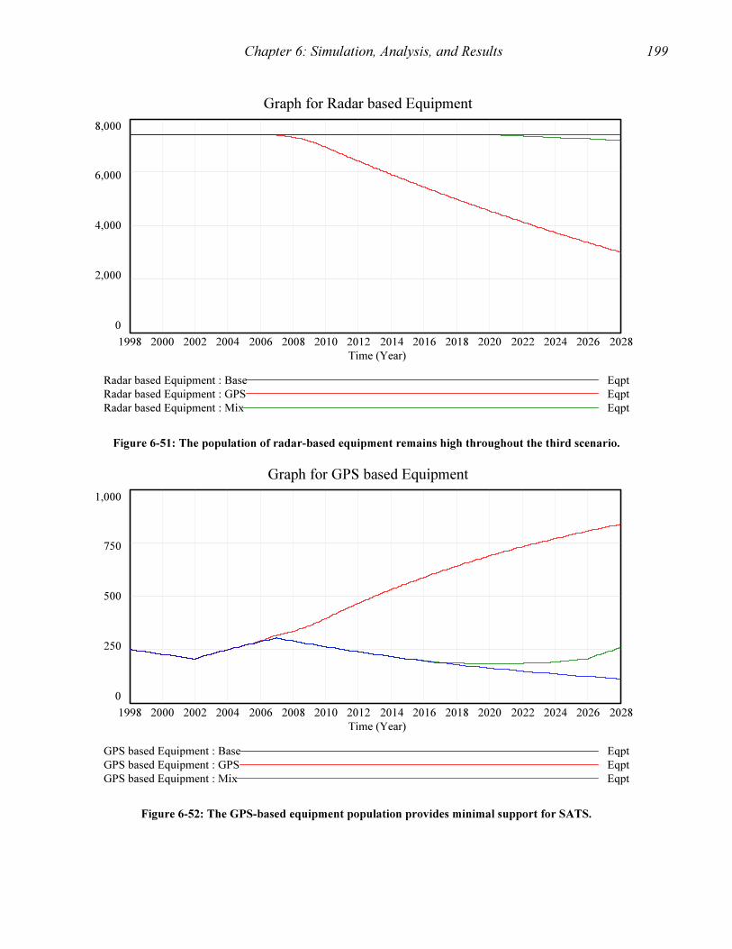
Chapter 6: Simulation, Analysis, and Results 199
Graph for Radar based Equipment
8,000
6,000
4,000
2,000
0
1998 2000 2002 2004 2006 2008 2010 2012 2014 2016 2018 2020 2022 2024 2026 2028
Time (Year)
Radar based Equipment : Base Eqpt
Radar based Equipment : GPS Eqpt
Radar based Equipment : Mix Eqpt
Figure 6-51: The population of radar-based equipment remains high throughout the third scenario.
Graph for GPS based Equipment
1,000
750
500
250
0
1998 2000 2002 2004 2006 2008 2010 2012 2014 2016 2018 2020 2022 2024 2026 2028
Time (Year)
GPS based Equipment : Base Eqpt
GPS based Equipment : GPS Eqpt
GPS based Equipment : Mix Eqpt
Figure 6-52: The GPS-based equipment population provides minimal support for SATS.

Chapter 6: Simulation, Analysis, and Results 200
The model addresses two other key parts of the ATC system: aircraft and airports. Figure
6-53 to Figure 6-56 describe the populations of AC, AT, GA, and SATS aircraft. The growth of
AC aircraft in Figure 6-53 plateaus around 2010 as in the first scenario due to inherent capacity
constraints in the system. There is a slight reduction in the AC population after 2025 that has a
small effect on revenue for the ATC system. Similarly, there are small declinations in the
population of AT and GA aircraft also beginning approximately 2025 as depicted in Figure 6-54
and Figure 6-55. The number of SATS aircraft, depicted in Figure 6-56, grows rapidly due to
conversions of AT and GA aircraft into SATS aircraft, enabled by the mild growth of supporting
GPS infrastructure in the third scenario. However, the third scenario delays the growth of SATS
by about five years, compared to the aggressive second scenario.
Figure 6-57 and Figure 6-58 capture the changes in the population of SATS and non-
SATS airports. The non-SATS airports in Figure 6-57 continue to decline in number due to the
normal demise of public use airports. After 2015, many of the non-SATS airports converted into
SATS airports. The growth in SATS airports in Figure 6-58 during the third scenario enabled
the relatively small-scale establishment of the SATS as a transportation system comprised of
about 200 airports and 500 aircraft by 2025.
Graph for AC Aircraft
20,000
17,000
14,000
11,000
8,000
1998 2000 2002 2004 2006 2008 2010 2012 2014 2016 2018 2020 2022 2024 2026 2028
Time (Year)
AC Aircraft : Base Aircraft
AC Aircraft : GPS Aircraft
AC Aircraft : Mix Aircraft
Figure 6-53: The third scenario maintains a steady population of AC aircraft.
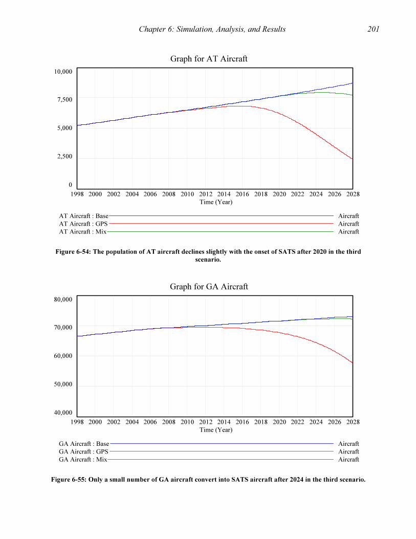
Chapter 6: Simulation, Analysis, and Results 201
Graph for AT Aircraft
10,000
7,500
5,000
2,500
0
1998 2000 2002 2004 2006 2008 2010 2012 2014 2016 2018 2020 2022 2024 2026 2028
Time (Year)
AT Aircraft : Base Aircraft
AT Aircraft : GPS Aircraft
AT Aircraft : Mix Aircraft
Figure 6-54: The population of AT aircraft declines slightly with the onset of SATS after 2020 in the third
scenario.
Graph for GA Aircraft
80,000
70,000
60,000
50,000
40,000
1998 2000 2002 2004 2006 2008 2010 2012 2014 2016 2018 2020 2022 2024 2026 2028
Time (Year)
GA Aircraft : Base Aircraft
GA Aircraft : GPS Aircraft
GA Aircraft : Mix Aircraft
Figure 6-55: Only a small number of GA aircraft convert into SATS aircraft after 2024 in the third scenario.
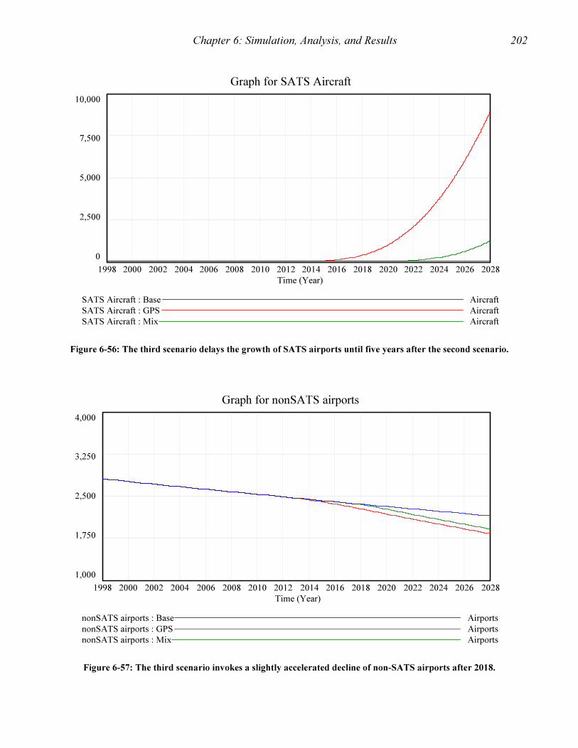
Chapter 6: Simulation, Analysis, and Results 202
Graph for SATS Aircraft
10,000
7,500
5,000
2,500
0
1998 2000 2002 2004 2006 2008 2010 2012 2014 2016 2018 2020 2022 2024 2026 2028
Time (Year)
SATS Aircraft : Base Aircraft
SATS Aircraft : GPS Aircraft
SATS Aircraft : Mix Aircraft
Figure 6-56: The third scenario delays the growth of SATS airports until five years after the second scenario.
Graph for nonSATS airports
4,000
3,250
2,500
1,750
1,000
1998 2000 2002 2004 2006 2008 2010 2012 2014 2016 2018 2020 2022 2024 2026 2028
Time (Year)
nonSATS airports : Base Airports
nonSATS airports : GPS Airports
nonSATS airports : Mix Airports
Figure 6-57: The third scenario invokes a slightly accelerated decline of non-SATS airports after 2018.

Chapter 6: Simulation, Analysis, and Results 203
Graph for SATS Airports
400
300
200
100
0
1998 2000 2002 2004 2006 2008 2010 2012 2014 2016 2018 2020 2022 2024 2026 2028
Time (Year)
SATS Airports : Base Airports
SATS Airports : GPS Airports
SATS Airports : Mix Airports
Figure 6-58: The third scenario shifts the growth of SATS airports five years later than the second scenario.
6.4.2 Analysis of Scenario 3
The results of the ATC Resource Management Model for the third scenario showed that
the ATC system will continue to function almost as it has in the past, with minor exceptions in
the distant future. The minor exceptions to normal behavior patterns appear to foreshadow the
changes indicated in the second scenario. The third scenario is the only scenario of the three
containing high revenue rates and growth in SATS airports and aircraft. Thus, the third scenario
offers the SATS the best opportunity to establish itself and survive as a transportation system.
Additionally, the third scenario includes a viable radar-based ATC system that generates the
revenue needed to supply the AATF with the funds needed to operate the radar-based ATC
system and establish SATS.
The behavior of the SATS and non-SATS airports over time may provide additional
support to the growth of the SATS. Table 6-4 below provides an eighteen-year overview of the
ratio of non-SATS IFR aircraft per public use airport. The data in the bottom row of Table 6-4
shows a range of 21 to 32 non-SATS IFR aircraft for each public use airport. The number of

Chapter 6: Simulation, Analysis, and Results 204
public use airports available for IFR aircraft is approximately 52% of the total number of public
use airports, as discussed previously in Section 4.10. As the number of public use airports
diminishes and the number of non-SATS IFR aircraft increases, the ratio of aircraft to airports
begins to escalate as illustrated in Figure 6-59. In the third scenario, the ratio climbs above 40
non-SATS IFR aircraft per public use airport by the year 2026.
Concurrent to the increase in non-SATS aircraft per public use airport, the number of
SATS aircraft per SATS airport remained relatively low in the third scenario. Figure 6-60
depicts the ratio of SATS aircraft per SATS airport from 1998 to 2028. The graph shows that all
scenarios experience a ratio of up to 40 SATS aircraft per SATS airport when the SATS is in its
infancy between 2008 and 2020. At that time, the SATS aircraft population virtually equals the
SATS aircraft to SATS airport ratio because there is only one SATS airport until 2012 all three
scenarios. The denominator grows slowly under the third scenario until about 2018 when the
rate of new SATS airports begins accelerating as depicted in Figure 6-58 above. After 2020,
when the non-SATS aircraft to airport ratio climbs above 35, the SATS aircraft to SATS airport
ratio is less than 10. The potential “crowding” at non-SATS airports may serve as an incentive
to transition to the SATS aircraft and system.
Table 6-4: The number of IFR aircraft per public use airport ranged from 21 to 32 between 1980 and 1998.
Airports & Aircraft 1980 1985 1994 1995 1996 1998
Public Use Airports 4,814 5,858 5,474 5,415 5,389 5,352
Adjusted Public Use (52%) 2,503 3,046 2,846 2,816 2,802 2,783
GA IFR nonSATS Aircraft 81,102 69,590 56,694 56,895 61,896 66,453
AT IFR nonSATS Aircraft 3,800 4,100 3,900 5,190
Total IFR type Aircraft 81,102 69,590 60,494 60,995 65,796 71,643
IFR Acft per Pub Use Airport 17 12 11 11 12 13
IFR Acft per Adjusted Pub Use Airport 32 23 21 22 23 26
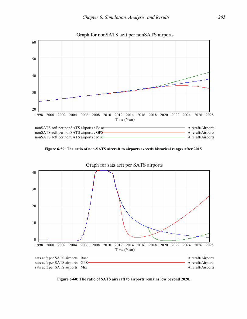
Chapter 6: Simulation, Analysis, and Results 205
Graph for nonSATS acft per nonSATS airports
60
50
40
30
20
1998 2000 2002 2004 2006 2008 2010 2012 2014 2016 2018 2020 2022 2024 2026 2028
Time (Year)
nonSATS acft per nonSATS airports : Base Aircraft/Airports
nonSATS acft per nonSATS airports : GPS Aircraft/Airports
nonSATS acft per nonSATS airports : Mix Aircraft/Airports
Figure 6-59: The ratio of non-SATS aircraft to airports exceeds historical ranges after 2015.
Graph for sats acft per SATS airports
40
30
20
10
0
1998 2000 2002 2004 2006 2008 2010 2012 2014 2016 2018 2020 2022 2024 2026 2028
Time (Year)
sats acft per SATS airports : Base Aircraft/Airports
sats acft per SATS airports : GPS Aircraft/Airports
sats acft per SATS airports : Mix Aircraft/Airports
Figure 6-60: The ratio of SATS aircraft to airports remains low beyond 2020.

Chapter 6: Simulation, Analysis, and Results 206
6.5 Summary of Simulation, Analysis, and Results
The three scenarios provided a glimpse of the future potential for the SATS. Each scenario
created a slightly different view of the future according to the resource management strategy
used to operate the ATC system. The discussion below describes the role of each scenario and
highlights the results of the simulations used to answer the research questions.
6.5.1 Research Question 1: Future levels of support for SATS under
radar-based ATC
The radar-based ATC scenario served as a base case from which to evaluate the current
trends in ATC. The scenario included a handful of SATS aircraft and SATS airports; however,
there was no management emphasis to provide resources to create the infrastructure needed to
support SATS. The purpose of this scenario was to determine system behavior if the managers
at the FAA chose to ignore the potential requirements of the SATS system and continue the
current radar-based method of conducting air traffic control.
The model created dynamic system behavior that captured growth in AATF revenue, FAA
budgets, facilities, and aircraft. The model illustrated the reduction of FAA employees, caused
by controller and maintainer retirements, and the system’s compensation through feedback to the
hiring and training functions. The model also described the decline of SATS aircraft and
systems as well as the continued decline in public use airports. The research showed that the
radar-based ATC system would not support a small fleet of SATS aircraft. Further analysis of
the behavior of the system indicated that the lack of SATS airports and ground-based GPS
equipment prohibited the establishment of the Small Aircraft Transportation System.
6.5.2 Research Question 2: Future levels of support for SATS under an
aggressive transition to GPS-based ATC
The GPS-based ATC scenario provided the opportunity to evaluate a major philosophical
change in the manner of ATC conducted by the FAA. However, a major constraint on the GPS-
based ATC scenario was to provide a moderate level of support to the many AC, AT, and GA
aircraft that continued to utilize the radar-based ATC system. Management emphasis was to
provide resources to create the infrastructure needed to support an aggressive expansion of GPS-

Chapter 6: Simulation, Analysis, and Results 207
based ATC, which supported the introduction and expansion of SATS aircraft. The purpose of
this scenario was to determine system behavior if the managers at the FAA chose to endorse the
SATS program while providing minimal support to the traditional radar-based ATC system.
The model demonstrated dynamic system behavior using the GPS-based approach that
proved to be unacceptable and infeasible. However, the research also showed that the
accelerated development of a GPS-based ATC system would support the establishment and
maturation of a system of SATS aircraft and airports. Further analysis of the behavior of the
ATC system indicated that the decline of AC aircraft caused an unacceptable reduction in system
revenue. Additionally, the large reduction of radar-based equipment in the system created the
potential for increased accidents or delays in the ATC system.
6.5.3 Research Question 3: Future levels of support for SATS under a
radar-based ATC system supplemented by GPS
The final ATC scenario provided the opportunity to evaluate a hybrid ATC system that
supported the radar-based approach while directing moderate amounts of resources towards GPS.
Management emphasis was to provide resources to maintain the infrastructure needed for radar-
based ATC while slightly accelerating the expansion of GPS-based ATC. The purpose of this
scenario was to determine system behavior if the managers at the FAA chose to rely primarily on
radar-based ATC, and, chose to provide a level of support to GPS related investments to give the
SATS program the opportunity to come into being.
The model demonstrated dynamic system behavior that appeared very similar to the first
scenario, yet provided sufficient marginal investments to elicit favorable trends for the SATS.
The research showed that by supplementing radar-based ATC with GPS-based infrastructure, the
system could produce over 250 SATS airports by 2028; beginning with only a dozen SATS
airports in 2018. Additionally, the research showed that the supplemental approach would create
a population of over 1,200 SATS aircraft by 2028; beginning with only 30 aircraft in 2020.
Further analysis of the behavior of the system indicated that the ratio of aircraft to airports would
encourage the transition to SATS aircraft due to the “overcrowding” of non-SATS aircraft.
All three scenarios provided evidence useful for drawing conclusions about the future
behavior of the ATC system. The data shows that SATS will thrive under the second scenario,
grow slowly under the third, and never come to fruition under the first. Additionally, the data

Chapter 6: Simulation, Analysis, and Results 208
shows that the AATF will support the ATC system under the first and third scenarios, but not the
second. Chapter 7 provides further discussion of the outcome of the scenario analysis above.

209
The FAA Operational Evolution Plan (FAA, 2002c) serves as the overarching document
that addresses the desire to expand NAS capacity and improve efficiency in accordance with
changing technology and adjustments in system priorities. However, the plan does not address
SATS, a potentially significant technological change to the NAS that may alter national aviation
priorities. The OEP focuses primarily on the larger airports around the nation that serve the
commercial airlines. The findings of this dissertation show that the transformation of several
hundred small airports in the US public use airport population can facilitate the growth of a
viable Small Aircraft Transportation System that complements the commercial airliner
dominated radar-based ATC system.
7.1 Major Findings
The most significant contribution of this research was the insight and understanding gained
of how several resource management strategies and the presence of SATS aircraft may impact
the future US Air Traffic Control system. In particular, the dissertation answered the
fundamental research question: what air traffic control resource management strategy will
support the future needs of the Small Aircraft Transportation System and create adequate tax
revenue to fund the Federal Aviation Administration? The research showed that a radar-based
ATC system, conservatively supplemented with GPS-based ATC capabilities, provided sustained
revenue for the AATF and the opportunity for the creation of a Small Aircraft Transportation
System.
The System Dynamics modeling and simulation methodology used to obtain the results
contributed to the body of knowledge in two ways. First, the methodology provided a macro
level view of the effects of feedback between the AATF and the ATC system. Second, the
methodology provided insight into the role of SATS aircraft in the dynamic behavior of a future
ATC system. The System Dynamics process guided the modeling effort. The process included
procedures to verify and validate the System Dynamics model. A product of the process was a
software tool that ATC resource managers could use to aid decision-making and understanding.
Chapter 7: Conclusion
Chapter 7: Conclusion 210
The ATC system performance results created by using the System Dynamics model provided the
data needed to answer the research questions.
7.2 Research Questions
The research questions stemming from the fundamental research question above helped
shape the scenarios addressed by the model in chapter 6 and led to understanding of the potential
future behavior of the ATC system. The first insight gained is that the continuation of the
current ground and radar-based ATC system will not create the conditions for the SATS to
succeed. The data generated by the model for the first scenario showed that SATS would be
nothing more than an experiment. The second insight gained is that too much emphasis on GPS-
based ATC will jeopardize the SATS because the lack of radar-based ATC will cause a decline
in AATF revenue. To create a viable SATS and maintain an adequate source of revenue, there
must be a balance between radar-based ATC and GPS-based ATC. Thus, the third insight
gained is that a future radar-based ATC system, supplemented by a ten-year transition period to
GPS, will provide adequate revenue to operate the ATC system and will set the conditions for
the successful establishment of the SATS. The second insight is counterintuitive, but makes
more sense in light of the third insight. The insights lead to actions resource managers at the
FAA should consider undertaking to shape the future ATC system.
7.3 Future FAA Resource Management Strategies
The focus of this effort was on the relationship between the GPS-based ATC system
required to support a network of SATS aircraft and the FAA resource management strategies that
would create the conditions for the existence of such a system. The System Dynamics modeling
process highlighted the challenges faced by managers who would have to reduce their level of
support for the existing radar-based ATC system in order to expand GPS. The results of the
research showed that it is possible to support both systems and meet the requirements of the
Airport and Airways Trust Fund. The results supported a strategy of choosing a conservative
migration of up to 25% of the funding available in the Facilities and Equipment account over a
ten-year period. The recommended strategy caused both Grants-in-Aid investments in SATS
airports and the expansion of the SATS aircraft population, resulting in an operational SATS.
Chapter 7: Conclusion 211
Managers at the FAA should also consider several other proposals regarding future
resource management and the SATS. First, the FAA should integrate SATS into the Operational
Evolution Plan (FAA, 2002c). The US Congress and NASA support SATS. The FAA should
not ignore the possibilities and potential of the SATS. The system may benefit the FAA. For
example, SATS could reduce requirements for Air Traffic Controllers at a time when there may
be controller shortages due to retirements. Second, the FAA should use the ATC resource
management model to observe how the ATC system will behave after they implement policy
decisions related to SATS. Managers can determine which parts of the system they may have
the most leverage in order to restructure it to create more favorable outcomes.
The FAA managers should take action in several areas. First, they should write an
Operational Evolution Plan for the SATS to address specific requirements for SATS aircraft.
Second, they should collect and process data to determine how GPS systems influence ATC. In
particular, they should determine how the reliability of the system may influence the need for Air
Traffic Controllers. Third, they should assess the impact of various tax rates on the AATF to
determine if SATS aircraft should fall into a unique tax category. Fourth, they should analyze
the future required distribution of resources among the major accounts of the FAA budget.
Finally, they should consider the impact of other emerging ATC technologies they may be more
advantageous than GPS.
Historically, restructuring the FAA has been a slow and methodical process due to the
conservative culture of the organization. The understanding created by System Dynamics
modeling may serve as an impetus to accelerate change with confidence. The findings of this
research indicate that the SATS faces a “limits to growth” system archetype depicted below in
Figure 7-1. Risk averse ATC resource managers can apply the archetype and the ATC Resource
Management Model to understand that SATS will grow continuously with increased funding for
GPS-based ATC. However, the constraint caused by the radar-based system upon the revenue
from AC aircraft clearly balances the growth of SATS. Tracing causality through the archetype
makes it easy to understand how SATS can grow or decline.
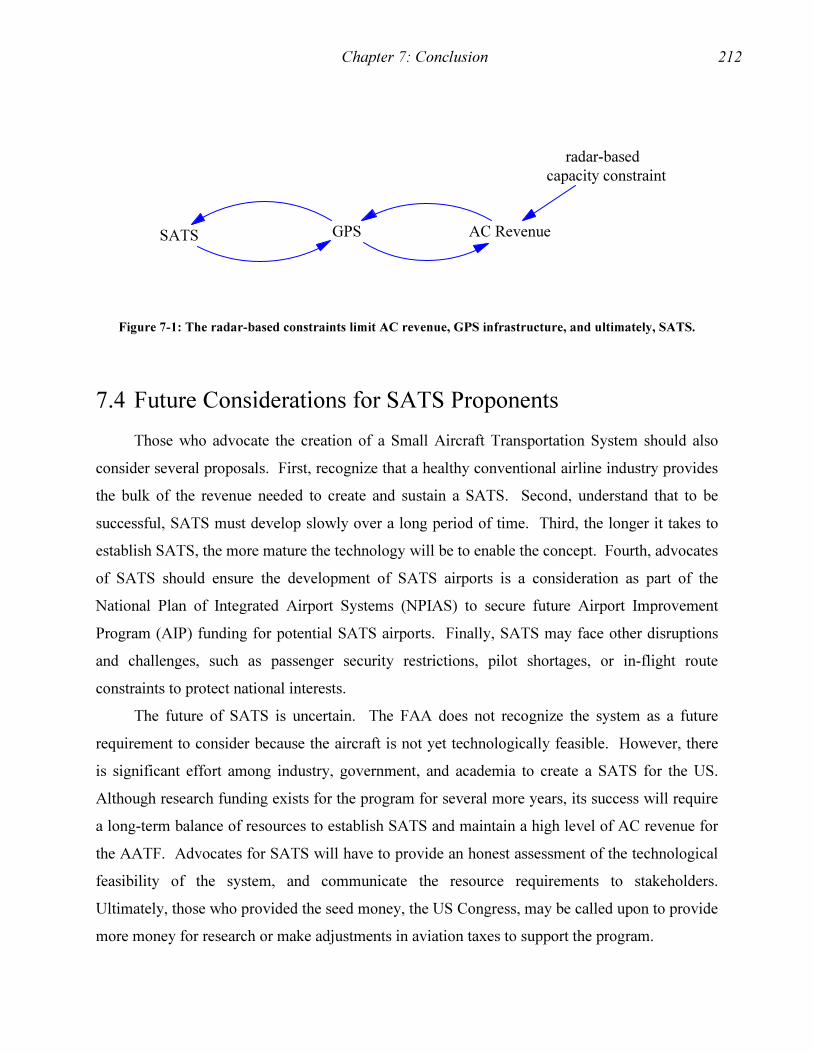
Chapter 7: Conclusion 212
SATS GPS AC Revenue
radar-based
capacity constraint
Figure 7-1: The radar-based constraints limit AC revenue, GPS infrastructure, and ultimately, SATS.
7.4 Future Considerations for SATS Proponents
Those who advocate the creation of a Small Aircraft Transportation System should also
consider several proposals. First, recognize that a healthy conventional airline industry provides
the bulk of the revenue needed to create and sustain a SATS. Second, understand that to be
successful, SATS must develop slowly over a long period of time. Third, the longer it takes to
establish SATS, the more mature the technology will be to enable the concept. Fourth, advocates
of SATS should ensure the development of SATS airports is a consideration as part of the
National Plan of Integrated Airport Systems (NPIAS) to secure future Airport Improvement
Program (AIP) funding for potential SATS airports. Finally, SATS may face other disruptions
and challenges, such as passenger security restrictions, pilot shortages, or in-flight route
constraints to protect national interests.
The future of SATS is uncertain. The FAA does not recognize the system as a future
requirement to consider because the aircraft is not yet technologically feasible. However, there
is significant effort among industry, government, and academia to create a SATS for the US.
Although research funding exists for the program for several more years, its success will require
a long-term balance of resources to establish SATS and maintain a high level of AC revenue for
the AATF. Advocates for SATS will have to provide an honest assessment of the technological
feasibility of the system, and communicate the resource requirements to stakeholders.
Ultimately, those who provided the seed money, the US Congress, may be called upon to provide
more money for research or make adjustments in aviation taxes to support the program.

Chapter 7: Conclusion 213
7.5 Future Research
This research successfully developed a System Dynamics model of the principal
components of the US air traffic control system. Future research may provide useful expansions
and extensions of the System Dynamics modeling approach. By developing stocks and flows
associated with the hub and spoke system, future researchers could expand the model to gain
greater insight on the flow of passengers through the system and how their feedback influences
the system. Additionally, an expanded model could be a useful tool to determine the impact
SATS may have upon the number of small aircraft utilizing the large hub airports. Researchers
could investigate how SATS may increase or reduce problems of congestion, parking shortages,
gate shortages, and wake vortex incidents.
Future research could extend the System Dynamics model of the ATC system by
generalizing it to other similar systems. The Federal Highway Trust Fund creates revenue based
on motor vehicle gasoline taxes. Department of Transportation managers may wish to
implement resource management strategies that impact revenue and non-fossil fuel vehicles.
Extending the ATC Resource Management Model to other domains may help managers
understand systems so they can make appropriate interventions with confidence.
7.6 Summary
The Small Aircraft Transportation System offers exciting opportunities on many fronts.
The technological challenges of developing a low-cost, yet highly capable means of airborne
transportation is being addressed by the aviation industry. Several academicians are addressing
the challenges of airspace management and Air Traffic Control under an approach that leads to
the notion of free flight. Program leadership and management emanates from NASA research
centers. However, the FAA has not taken the initiative to support the SATS concept. The
research in this dissertation attempts to bridge a gap that exists between the FAA and the
communities and groups who support the SATS program. The research shows that an ATC
system that supports SATS is feasible, however, the FAA must join with the stakeholders to
create the conditions to make the ATC piece of the SATS a success.

214
Ball, J. (1997) Free Flight an Air Traffic Management Partnership. Digital Avionics Systems
Conference, 1997. 9.1-9 – 9.1-15. Available: http://ieeexplore.ieee.org/lpdocs/epic03/ Barrer, J. (1999) Using Path Objects for Air Traffic Control. McLean, VA: The Mitre Corporation. Barrett, J. & Beck, K. (2001) People – The Key to Success. Air Traffic Technology
International. London: UK & International Press. Blanchard, B. & Fabrycky, W. (1998) Systems Engineering and Analysis. Upper Saddle River, New Jersey: Prentice Hall. Bureau of Labor Statistics (2002) Air Traffic Controllers. Available: http://www.bls.gov/oco/ocos108.htm Bureau of Transportation Statistics (2002) General Aviation Profile. Available: http://www.bts.gov/btsprod/nts/ Campbell, D (2001) The Long and Winding (and Frequently Bumpy) Road to Successful Client Engagement: One Team’s Journey. System Dynamics Review, 17(3): 195-215. Churchman, C. (1968) The Systems Approach, New York: Dell Publishing Co. Chwif, L., Barretto, M. & Paul, R. (2000) On Simulation Model Complexity. Proceedings of the
2000 Winter Simulation Conference. Orlando, Florida Coyle, R. (1996) System Dynamics Modelling: A Practical Approach. London: Chapman & Hall. Dempsey, P. (2000) Airport Planning and Development Handbook: A Global Survey. New York: McGraw-Hill. Department of Transportation (2000). A Preliminary Design Process for Airspace Systems.
Washington, D.C. Department of Transportation (1999). National Plan of Integrated Airport Systems.
Washington, D.C. Doyle, J. & Ford, D. (1998) Mental Models Concepts for System Dynamics Research. System
Dynamics Review, 14(1): 3-29. Eby, M. and Kelly, W. (1999) Free Flight Separation Assurance Using Distributed Algorithms. Unpublished Paper. Available: http://www.sourcecodesystems.com
References

References 215
Eclipse Aviation (2001) Nimbus Group Awards Eclipse Aviation Order for 1,000 Aircraft. Albuquerque, New Mexico: 17 September 2001 Press Release. Available: http://sats.erau.edu/News/eclipse_091701.htm Farrell, C. (2002) A Modeling and Simulation Approach to the Small Aircraft Transportation
System (SATS): Assessing Midair Conflict Risk Under the Free-Flight Paradigm. Unpublished Master’s Thesis. Virginia Polytechnic Institute and State Univesity. Federal Aviation Administration (2002a). Administrator’s Fact Book. Washington, D.C.: Department of Transportation. Available: http://www.atctraining.faa.gov/site/ Federal Aviation Administration (2002b). Air Traffic Activity Data System (ATADS). Washington, D.C.: DOT. Available:http://www.apo.data.faa.gov/atads/ Federal Aviation Administration (2002c). Operational Evolution Plan 4.0. Washington, D.C.: Department of Transportation. Available:http://www.faa.gov/programs/oep Federal Aviation Administration (2002d). Job Vacancy Announcement. Washington, D.C.: Department of Transportation. Available:http://www.faa.gov/careers/employment Federal Aviation Administration (2000). Gate to Gate Multimedia CD ROM. Washington, D.C.: Department of Transportation Federal Aviation Administration (2000b). Air Traffic Services Plan. Washington, D.C.: Department of Transportation Federal Aviation Administration (2001). Federal Aviation Administration Budget in Brief, Washington, D.C.: Department of Transportation. Available: http://www.faa.gov/aba/html_budget/files_pdf/bib2001.pdf Federal Aviation Administration (2001b). Federal Aviation Administration FY 2001 Financial
Statement, Washington, D.C.: Department of Transportation. Available: http://www.faa.gov/aba/ Federal Aviation Administration (2001c). National Airspace System Capital Investment Plan
Fiscal Years 2002-2006, Washington, D.C.: Department of Transportation. Available: http://www.faa.gov/ Federal Aviation Administration (1999). National Airspace System Architecture Version 4.0, Washington, D.C.: Department of Transportation. Available: http://www.faa.gov/nasarchitecture/version4.htm Federal Aviation Administration (2002). FAA Order 7210.3, Facility Operation and
Administration, Washington, D.C.: Department of Transportation. Available: http://www.faa.gov/atpubs
References 216
Federal Aviation Administration (1997). Statistical Handbook of Aviation. Washington, D.C.: Department of Transportation. Available: http://www.api.faa.gov/handbook96/toc96.htm Ford, A. (1999) Modeling the Environment: An Introduction to System Dynamics Modeling of
Environmental Systems. Washington, D.C.: Island Press. Forrester, J. (1998) Designing the Future. Speech given at the Universidad de Sevilla, December 15, 1998. Forrester, J. (1994) System Dynamics, System Thinking, and Soft OR. System Dynamics
Review, 10(2-3): 245-255. Forrester, J. (1991) System Dynamics and the Lessons of 35 Years. A Chapter for K. De Greene (Ed.), The Systemic Basis of Policy Making in the 1990s. Forrester, J. (1971) Principles of Systems. New York: Wright-Allen Press, Inc. Forrester, J. (1961) Industrial Dynamics. Cambridge, Massachusetts: The MIT Press. Government Accounting Office (2002). GAO Report 02-591 Air Traffic Control, Washington, D.C.: Available: http://www.gao.gov/new.items/d02591.pdf Hoekstra, J., van Gent, R. and Ruigrok, R. (1998) Man-in-the-Loop Part of a Study Looking at a Free Flight Concept. Digital Avionics Systems Conference, 1998. F56-1 – F56-8. Available:http://ieeexplore.ieee.org Holmes, B. (2000a) Friends of Meigs Field Presentation, Chicago, IL: January 28, 2000. Available: http://sats.nasa.gov/Pages/satsarchive.html Holmes, B. (2000b) Testimony before Subcommittee on Aviation, Committee on Transportation
and Infrastructure, House of Representatives, Washington, D.C.: May 16, 2000. Available: http://sats.nasa.gov/Pages/satsarchive.html Homer, J. (1996) Why we Iterate: Scientific Modeling in Theory and Practice. System Dynamics
Review, 12(1): 1-19. Illman, P. (1999) The Pilot’s Air Traffic Control Handbook. New York, New York: McGraw- Hill. Keating, E., Oliva, R., Repenning, N., Rockart, S. & Sterman, J. (1999) Overcoming the Improvement Paradox. European Management Journal, 17(2): 120-134. Keogh, M. and Doman, A. (1992) The CEO as Organization Designer: An Interview with
Professor Jay W. Forrester. The McKinsey Quarterly, (2): 3-30. Available: http://www.mckinseyquarterly.com
References 217
Klein, K., Dansereau, F., & Hall, R. (1994) Levels Issues in Theory Development, Data Collection, and Analysis. Academy of Management Review, 19(2), 195-229. Lammes, M. (2002) Hawthorne Automated Flight Service Station Homepage. Available: http://www.faa.gov/ats/hhrafss/index.htm Law, A., Kelton, W. (2000) Simulation Modeling and Analysis. Boston: McGraw Hill. Leedy, P. & Ormrod, J. (2001) Practical Research: Planning and Design. Upper Saddle River, New Jersey: Prentice-Hall, Inc. Lyneis, J. (2000) System Dynamics for Market Forecasting and Structural Analysis. System
Dynamics Review, 16(1): 3-25. Lyneis, J. (1999) System Dynamics for Business Strategy: A Phased Approach. System
Dynamics Review, 15(1): 37-70. Maani, K. & Cavana, R. (2000) Systems Thinking and Modelling – Understanding Change and
Complexity. New Zealand: Pearson Education. NASA (2000a) Small Aircraft Transportation System (SATS) Program Planning White Paper. Langley, Virginia: General Aviation Program Office. NASA (2000b) Request for Information: Small Aircraft Transportation System (SATS) Program
Partnership. Langley, Virginia: General Aviation Program Office. Nolan, M. (1999) Fundamentals of Air Traffic Control. Pacific Grove, California: Brooks/Cole Publishing Company. O’Connor, J. & McDermott, I. (1997) The Art of Systems Thinking. San Francisco: Thorsons. Odum, E. (1971) Fundamental of Ecology. Philadelphia: Saunders College Publishing. Pappas, G., Tomlin, C., Lygeros, J., Godbole, D., & Sastry, S. (1997) A Next Generation Architecture for Air Traffic Management Systems. Proceedings of the 36
th Conference on
Decision & Control, 2405-2410. Peterson, D. & Eberlein, R. (1994) Reality Check: A Bridge Between Systems Thinking and System Dynamics. System Dynamics Review, 10(2-3): 159-173. Richmond, B. (1993) Systems Thinking: Critical Thinking Skills for the 1990s and Beyond. System Dynamics Review, 9(2): 113-133. Senge, P. (1990) The Fifth Discipline: The Art and Practice of the Learning Organization. New York: Doubleday.

References 218
Senge, P., Kleiner, A., Roberts, C., Ross, R. & Smith, B. (1994) The Fifth Discipline Fieldbook:
Strategies and Tools for Building a Learning Organization. New York: Doubleday. Schrage, Michael. (2000) Serious play: How the world’s best companies simulate to innovate. Boston: Harvard Business School Press. Skoniezki, A. (2001) Controller Shortage Situation in Europe. The Controller. 40(4): 6-9. Small Aircraft Transportation System Program Planning White Paper. National Aeronautics and
Space Administration. Langley Research Center, Langley Air Force Base, VA: September 19, 2000. Available: http://sats.nasa.gov/Pages/satsarchive.html Smith, P., Billings, C., Woods, D. & McCoy, C. (1998) Human Factors Issues in a Future Air Traffic Management System. Proceedings of the 17
th Digital Avionics Systems
Conference, 2, F55-1 – F55-7. Sterman, J. (2001) System Dynamics Modeling: Tools for Learning in a Complex World. California Management Review, 43(4): 8-25. Sterman, J. (2000) Business Dynamics: Systems Thinking and Modeling for a Complex World. Boston: McGraw-Hill Publishing. Sterman, J. (1994) Learning in and About Complex Systems. System Dynamics Review, 10(2-3): 291-330. Suiter, R. & Petersen, D. (2001) Federal Aviation Administration Performance Based Organization Strategic Decision Support System. Suiter and Associates, FAA Contract DTFA 01-00-C-00068. System Dynamics Society (2001) available at http://www.albany.edu/cpr/sds/ Tomlin, C., Pappas, G. & Sastry, S. (1998) Conflict Resolution for Air Traffic Management: A Study in Multiagent Hybrid Systems. IEEE Transactions on Automatic Control, 43(4), 509-521. Trani, A. (2002) VA SATS Transportation Report. Blacksburg, VA: Virginia Polytechnic Institute and State University. Available at http://128.173.204.63/vasats_index.html
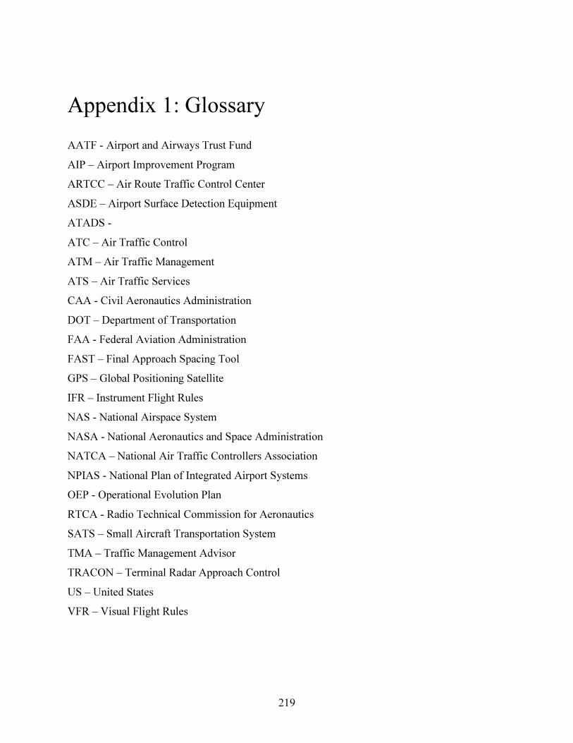
219
AATF - Airport and Airways Trust Fund
AIP – Airport Improvement Program
ARTCC – Air Route Traffic Control Center
ASDE – Airport Surface Detection Equipment
ATADS -
ATC – Air Traffic Control
ATM – Air Traffic Management
ATS – Air Traffic Services
CAA - Civil Aeronautics Administration
DOT – Department of Transportation
FAA - Federal Aviation Administration
FAST – Final Approach Spacing Tool
GPS – Global Positioning Satellite
IFR – Instrument Flight Rules
NAS - National Airspace System
NASA - National Aeronautics and Space Administration
NATCA – National Air Traffic Controllers Association
NPIAS - National Plan of Integrated Airport Systems
OEP - Operational Evolution Plan
RTCA - Radio Technical Commission for Aeronautics
SATS – Small Aircraft Transportation System
TMA – Traffic Management Advisor
TRACON – Terminal Radar Approach Control
US – United States
VFR – Visual Flight Rules
Appendix 1: Glossary

220
The following table provides the average annual number of control tower operations for
the four types of control towers.
LOCID: Control tower location identifiers.
FTYPE: Type of control tower; B – radar, C – limited radar, D – non-rader, E – VFR, F –
Contract VFR
AC Avg: Average annual control tower operations between 1990-2001 for Air Carrier aircraft
AT Avg: Average annual control tower operations between 1990-2001 for Air Taxi aircraft
GA Avg: Average annual control tower operations between 1990-2001 for General Aviation
aircraft
MIL Avg: Average annual control tower operations between 1990-2001 for Military aircraft
Rank: Quantitative order for the LOCID and type aircraft.
LOCID FTYPE AC Avg AC Rank AT Avg AT Rank GA Avg GA Rank MIL Avg MIL Rank
ORD C 697,445 1 142,618 10 33,144 252 2,235 163
DFW C 592,092 2 204,886 2 34,398 238 790
ATL B 573,176 3 170,984 4 21,868 351 2,851 140
LAX C 479,061 4 207,493 1 32,992 256 6,767 53
PHX C 341,817 5 83,538 27 88,060 53 7,541 43
DEN C 334,389 6 139,584 11 25,728 315 1,245
STL C 317,303 7 120,166 15 32,878 257 6,763 54
DTW C 316,170 8 107,729 19 66,435 91 1,494
EWR C 314,068 9 101,631 21 19,742 373 317
SFO C 313,477 10 83,428 28 25,458 317 2,483 152
MIA B 305,824 11 134,656 12 72,108 84 6,399 60
IAH C 278,943 12 79,484 31 31,400 269 887
MSP C 269,328 13 108,681 17 77,014 74 3,057 136
LAS C 262,693 14 66,697 40 90,302 46 17,734 10
CLT B 260,800 15 131,052 14 62,298 99 4,136 101
LGA C 256,314 16 79,812 30 18,056 390 312
PIT B 253,528 17 149,139 9 23,760 333 6,792 50
BOS C 247,846 18 202,506 3 32,674 260 632
Appendix 2: Control Tower Rankings

Appendix 2: Control Tower Rankings 221
PHL B 240,593 19 133,287 13 50,036 148 4,225 99
JFK C 223,698 20 107,859 18 14,729 416 614
SEA C 216,978 21 157,397 8 7,374 450 225
MCO B 210,534 22 88,040 23 29,322 287 5,223 76
CVG B 190,803 23 160,698 6 19,708 374 1,376
MEM B 189,679 24 100,978 22 60,228 107 5,519 72
DCA B 180,299 25 76,089 33 55,452 119 6,370 61
SLC C 174,877 26 85,687 24 79,278 69 4,303 97
BWI B 162,830 27 80,726 29 33,496 245 2,191 165
SAN C 143,128 28 52,552 49 18,912 382 3,793 113
CLE B 142,965 29 105,403 20 31,635 268 3,098 133
OAK C 138,986 30 53,382 47 149,157 12 686
MCI B 132,136 31 49,317 50 14,187 421 990
TPA B 128,766 32 78,289 32 44,685 170 1,929 180
MDW C 125,517 33 60,636 42 76,166 76 1,955 178
HOU C 120,756 34 16,590 140 113,798 24 644
SJC C 117,401 35 25,874 95 96,741 40 574
IND B 115,017 36 72,272 37 50,980 140 2,097 170
BNA B 114,714 37 73,375 36 65,315 95 5,042 80
PDX C 114,274 38 119,459 16 45,326 166 10,509 28
RDU B 113,305 39 75,864 35 69,284 86 6,012 66
IAD B 111,876 40 167,178 5 57,185 116 6,776 52
FLL C 110,668 41 54,774 46 74,153 80 955
MSY B 102,887 42 29,202 84 25,973 310 1,965 176
DAL C 94,232 43 30,944 73 96,379 41 1,282
ONT C 94,135 44 29,308 83 25,416 318 303
SDF B 92,124 45 36,849 61 33,672 244 4,525 93
SAT B 81,352 46 32,974 69 107,240 33 7,202 46
MKE B 81,018 47 67,662 39 43,155 177 5,178 77
ABQ B 77,858 48 35,902 63 63,218 98 23,076 4
SJU C 77,643 49 84,152 25 26,916 302 3,470 121
AUS B 77,538 50 18,449 130 86,366 56 5,556 71
CMH B 75,257 51 67,734 38 52,505 135 1,398
SNA C 73,625 52 22,423 106 243,821 2 444
SMF E 73,148 53 33,958 68 26,225 308 1,388
DAY B 69,191 54 38,613 58 40,958 193 1,909 183
BDL C 67,036 55 53,381 48 41,750 185 7,921 34
RNO B 65,163 56 20,490 118 50,578 145 5,073 79
ELP B 57,418 57 10,359 209 54,188 124 4,801 85
BUR C 56,812 58 38,436 59 87,096 55 602
PBI B 55,674 59 29,530 81 105,847 34 1,389
BUF B 52,454 60 39,796 54 38,290 212 3,345 128
JAX B 51,961 61 33,964 67 28,294 295 8,246 32
TUL B 49,215 62 16,042 147 75,028 77 21,065 7
OKC B 48,367 63 11,697 192 60,757 105 25,972 2
GSO B 46,575 64 25,121 98 52,172 136 850
OMA C 45,334 65 29,015 86 51,314 138 889

Appendix 2: Control Tower Rankings 222
TUS C 43,137 66 11,005 200 93,531 45 23,788 3
ROC B 41,923 67 43,785 51 43,163 176 2,121 167
ORF B 40,750 68 23,617 101 59,263 110 3,972 105
RSW B 39,728 69 14,205 160 10,020 441 1,344
RIC B 39,379 70 29,495 82 50,283 146 10,204 30
GEG B 38,616 71 35,684 64 24,489 329 1,752 186
SYR B 36,928 72 59,655 43 36,129 221 5,570 70
BHM B 36,560 73 26,711 93 74,159 79 10,394 29
PVD B 36,487 74 41,223 52 41,918 181 3,068 134
LIT B 34,904 75 21,295 113 78,109 71 7,212 45
COS B 31,428 76 11,928 190 54,763 122 16,681 12
BOI B 31,280 77 29,671 80 61,448 104 11,946 23
DSM B 30,137 78 27,994 92 55,197 121 4,041 102
ICT B 26,449 79 18,274 131 98,807 39 2,084 171
ALB B 26,220 80 65,277 41 42,852 178 4,632 90
GRR B 23,843 81 34,945 65 52,633 132 1,167
TYS B 22,602 82 26,582 94 53,087 129 12,433 21
CHS B 22,284 83 9,204 227 32,389 262 22,202 6
CAE B 20,600 84 24,077 99 38,387 211 3,967 106
GUM G 20,012 85 4,181 10,026 440 3,155 130
TOL B 19,869 86 20,134 120 32,809 258 3,792 114
MDT B 19,852 87 30,441 75 18,020 392 4,626 91
LBB B 19,759 88 15,415 153 31,816 266 2,414 156
MHT B 19,600 89 29,851 78 34,125 241 577
GSP B 18,394 90 19,827 122 18,587 385 1,454
SRQ C 18,100 91 13,303 177 94,767 44 2,065 172
JAN B 17,688 92 17,428 134 22,817 343 7,889 36
ABE B 16,824 93 20,159 119 50,961 141 2,492 151
MSN B 16,651 94 15,754 149 53,829 125 6,158 64
HSV B 16,601 95 10,346 210 28,396 294 4,786 86
PWM B 16,008 96 31,249 72 35,672 225 1,550 195
SAV B 15,480 97 9,354 223 40,973 192 6,782 51
FWA B 15,358 98 22,703 104 34,692 235 3,824 109
CID B 14,823 99 17,229 136 30,860 275 216
MAF B 14,471 100 9,243 226 21,605 354 6,278 62
PNS C 14,266 101 21,931 109 33,870 243 20,752 8
CRP B 13,803 102 14,355 159 32,306 264 13,377 20
LGB E 13,511 103 4,153 192,219 4 1,320
HRL G 13,456 104 3,874 11,910 434 4,211 100
ISP C 13,270 105 22,099 108 78,776 70 2,444 155
LEX B 13,094 106 22,446 105 47,305 160 1,297
SBN B 12,957 107 21,172 114 26,375 305 169
SHV B 12,711 108 25,666 96 25,872 311 3,818 110
MOB B 12,689 109 7,700 248 23,120 338 22,670 5
BTR B 12,238 110 16,524 141 52,542 133 1,921 181
FSD B 11,634 111 16,288 144 36,443 218 4,350 96
MLI B 11,539 112 16,511 142 27,845 298 1,669 191

Appendix 2: Control Tower Rankings 223
SWF G 11,518 113 13,408 175 49,130 153 6,403 59
ACY B 11,481 114 16,145 145 33,090 253 12,278 22
BIL B 11,373 115 32,159 71 35,644 227 670
AMA B 11,348 116 10,109 216 21,946 349 13,615 18
MYR B 11,301 117 12,945 180 20,116 367 1,615 194
FAT B 11,209 118 56,252 45 77,653 73 9,925 31
GRB B 10,810 119 12,868 182 21,908 350 815
HPN C 10,527 120 39,242 57 110,552 29 287
MWH B 10,499 121 4,769 294 24,558 327 3,136 131
TLH B 10,049 122 33,975 66 43,786 173 4,931 83
MHR G 9,955 123 13,803 168 29,180 288 3,976 104
YIP E 9,753 124 29,686 79 43,372 175 368
CHA B 9,187 125 15,648 151 50,761 144 3,794 112
BTV B 9,040 126 39,542 56 30,921 274 6,756 55
ROA B 8,931 127 28,609 89 29,515 286 949
DAB B 8,801 128 4,511 297 227,264 3 822
CAK B 8,630 129 19,576 124 54,689 123 4,915 84
PIA B 8,572 130 20,922 116 30,216 280 6,725 56
ATW G 8,554 131 12,643 185 22,825 342 32
SGF B 8,465 132 21,684 112 38,811 210 3,987 103
LAN B 8,309 133 29,158 85 41,653 186 1,621 193
PSP B 8,280 134 30,326 77 44,111 171 628
BFI E 8,267 135 36,594 62 191,848 5 2,117 168
MBS B 8,186 136 10,220 215 20,579 360 506
GTF B 8,098 137 13,808 167 16,614 404 5,876 67
BGR B 7,747 138 22,800 103 22,487 345 10,721 26
ASE B 7,650 139 5,554 280 26,311 306 120
RFD B 7,490 140 11,970 189 43,857 172 1,156
RST B 7,417 141 3,231 24,973 321 1,390
STT C 7,342 142 58,716 44 21,634 353 1,919 182
PIE C 7,203 143 5,472 281 78,094 72 8,049 33
MLB G 7,130 144 2,509 88,667 51 613
CWA G 6,937 145 11,083 197 10,515 438 475
SBA B 6,894 146 41,153 53 71,910 85 1,011
LNK B 6,860 147 10,896 202 39,104 208 10,849 25
MFE G 6,758 148 2,660 28,949 290 3,869 108
TRI B 6,644 149 15,676 150 36,099 222 512
FAR B 6,551 150 11,117 196 34,271 240 4,442 95
CRW B 6,496 151 25,291 97 36,228 219 3,949 107
GSN G 6,466 152 23,652 100 8,797 446 450
AZO B 6,390 153 19,378 126 39,598 205 390
EUG B 6,122 154 22,266 107 49,110 154 1,542 196
MGM B 5,994 155 10,533 205 31,899 265 17,086 11
AVL B 5,941 156 13,827 165 34,687 236 1,810 185
AVP B 5,833 157 15,418 152 25,275 319 1,292
AGS B 5,508 158 8,436 236 18,851 383 3,201 129
DET G 5,066 159 7,638 249 65,218 96 406

Appendix 2: Control Tower Rankings 224
MSO G 5,056 160 11,348 194 23,050 341 391
FNT B 5,044 161 17,344 135 31,191 271 353
BZN G 4,876 162 5,136 286 18,026 391 322
DLH B 4,795 163 6,566 264 20,565 361 5,237 75
FAY B 4,658 164 10,364 208 23,222 336 6,916 49
MLU B 4,544 165 9,929 219 29,164 289 2,808 141
ILM B 4,453 166 13,783 170 30,769 276 2,463 154
STX G 4,354 167 28,993 87 6,007 2,016 174
BIS B 4,188 168 11,216 195 24,841 323 2,668 145
HTS B 3,998 169 8,804 229 20,720 358 647
XNA G 3,925 170 19,793 123 5,629 819
GCN E 504 159,590 7 6,325 184
ACK E 67 83,929 26 46,199 162 756
HYA G 4 76,080 34 25,829 313 108
LFT B 1,181 39,707 55 35,578 229 2,102 169
HUM G 0 37,936 60 17,343 397 381
EYW G 806 32,787 70 36,573 216 7,766 39
VGT E 2 30,814 74 61,615 103 147
TEB C 113 30,371 76 185,589 6 368
BFL B 1,306 28,819 88 68,990 87 1,370
EVV B 1,674 28,535 90 32,399 261 767
MRY B 2,663 28,201 91 56,025 118 1,679 190
PSC B 2,605 23,008 102 25,551 316 766
CHO G 592 21,888 110 32,364 263 1,357
MVY G 5 21,732 111 29,909 282 185
SPI B 395 20,970 115 42,524 179 5,266 74
BGM B 2,648 20,764 117 14,244 420 546
GJT G 2,565 19,942 121 38,953 209 2,734 143
BLI G 1,102 19,563 125 35,896 224 801
PHF E 2,364 19,375 127 53,438 127 15,507 13
AGC E 15 19,146 128 73,529 81 604
MFR G 2,496 18,809 129 24,641 324 337
PFN G 2,664 18,079 132 33,166 251 2,357 159
TVC E 2,619 17,736 133 40,083 200 2,642 146
APA E 9 16,990 137 173,820 8 1,443
CMI B 1,206 16,953 138 39,817 202 518
FMN G 48 16,853 139 29,557 285 328
BPT B 25 16,439 143 17,220 399 1,378
ALO B 217 16,044 146 23,063 340 2,757 142
LCH B 17 15,759 148 15,781 410 1,733 188
SBP G 1 15,396 154 40,113 199 705
RDD G 67 15,164 155 35,161 232 777
OXR G 38 14,963 156 40,367 197 1,230
ARA G 129 14,797 157 8,600 447 6,160 63
PIH G 166 14,383 158 17,380 396 223
MFR E 2,496 14,194 161 24,641 325 337
ORL E 0 14,181 162 118,569 21 965
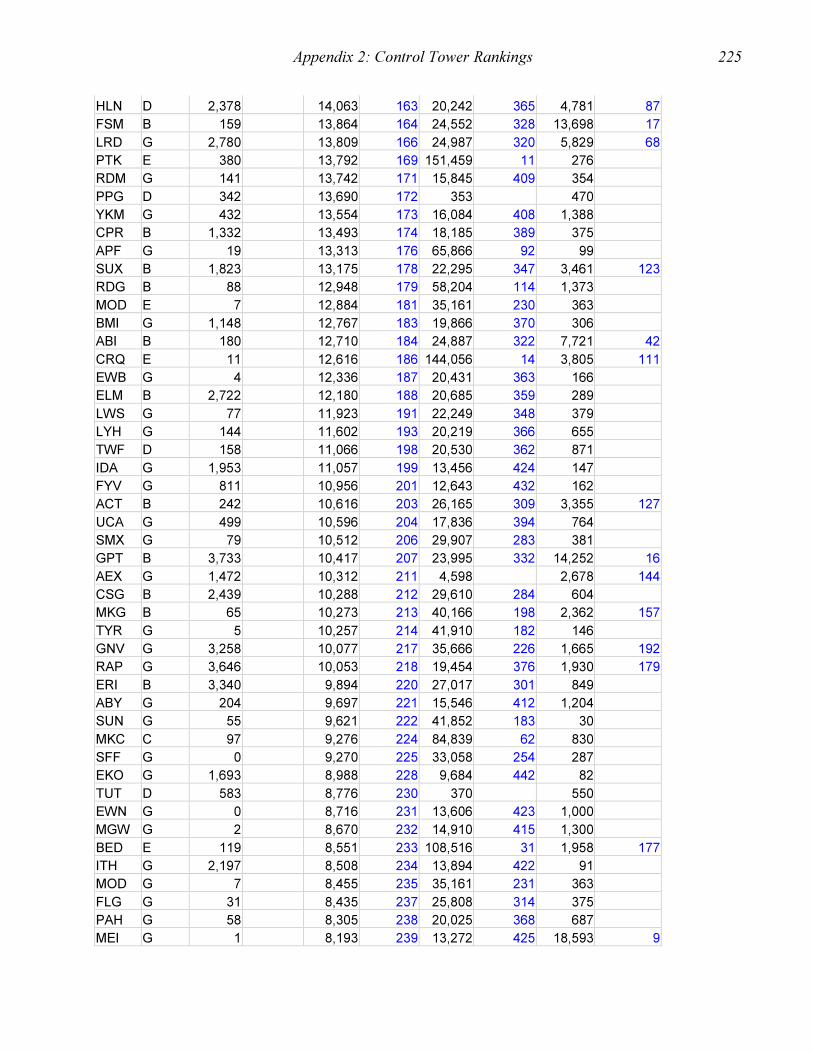
Appendix 2: Control Tower Rankings 225
HLN D 2,378 14,063 163 20,242 365 4,781 87
FSM B 159 13,864 164 24,552 328 13,698 17
LRD G 2,780 13,809 166 24,987 320 5,829 68
PTK E 380 13,792 169 151,459 11 276
RDM G 141 13,742 171 15,845 409 354
PPG D 342 13,690 172 353 470
YKM G 432 13,554 173 16,084 408 1,388
CPR B 1,332 13,493 174 18,185 389 375
APF G 19 13,313 176 65,866 92 99
SUX B 1,823 13,175 178 22,295 347 3,461 123
RDG B 88 12,948 179 58,204 114 1,373
MOD E 7 12,884 181 35,161 230 363
BMI G 1,148 12,767 183 19,866 370 306
ABI B 180 12,710 184 24,887 322 7,721 42
CRQ E 11 12,616 186 144,056 14 3,805 111
EWB G 4 12,336 187 20,431 363 166
ELM B 2,722 12,180 188 20,685 359 289
LWS G 77 11,923 191 22,249 348 379
LYH G 144 11,602 193 20,219 366 655
TWF D 158 11,066 198 20,530 362 871
IDA G 1,953 11,057 199 13,456 424 147
FYV G 811 10,956 201 12,643 432 162
ACT B 242 10,616 203 26,165 309 3,355 127
UCA G 499 10,596 204 17,836 394 764
SMX G 79 10,512 206 29,907 283 381
GPT B 3,733 10,417 207 23,995 332 14,252 16
AEX G 1,472 10,312 211 4,598 2,678 144
CSG B 2,439 10,288 212 29,610 284 604
MKG B 65 10,273 213 40,166 198 2,362 157
TYR G 5 10,257 214 41,910 182 146
GNV G 3,258 10,077 217 35,666 226 1,665 192
RAP G 3,646 10,053 218 19,454 376 1,930 179
ERI B 3,340 9,894 220 27,017 301 849
ABY G 204 9,697 221 15,546 412 1,204
SUN G 55 9,621 222 41,852 183 30
MKC C 97 9,276 224 84,839 62 830
SFF G 0 9,270 225 33,058 254 287
EKO G 1,693 8,988 228 9,684 442 82
TUT D 583 8,776 230 370 550
EWN G 0 8,716 231 13,606 423 1,000
MGW G 2 8,670 232 14,910 415 1,300
BED E 119 8,551 233 108,516 31 1,958 177
ITH G 2,197 8,508 234 13,894 422 91
MOD G 7 8,455 235 35,161 231 363
FLG G 31 8,435 237 25,808 314 375
PAH G 58 8,305 238 20,025 368 687
MEI G 1 8,193 239 13,272 425 18,593 9

Appendix 2: Control Tower Rankings 226
TXK G 64 8,116 240 19,863 371 1,046
FLO B 1 7,967 241 21,748 352 1,725 189
YNG B 1,766 7,866 242 30,961 273 6,609 57
LSE G 2,118 7,840 243 15,758 411 516
JAC G 1,536 7,819 244 16,901 401 204
MYF E 5 7,795 245 130,209 18 267
STS E 66 7,789 246 85,401 61 556
FXE E 0 7,774 247 178,159 7 160
CLL G 70 7,637 250 27,711 299 7,091 47
SIG G 2 7,501 251 48,320 156 2,928 138
HVN G 805 7,483 252 28,489 293 200
OPF G 89 7,354 253 72,715 83 7,904 35
GFK E 3,584 7,124 254 81,439 66 671
CRG G 0 7,113 255 58,662 112 11,004 24
PDT G 12 7,067 256 18,554 386 1,366
GGG B 50 7,018 257 31,001 272 1,741 187
CKB B 15 6,852 258 22,573 344 3,462 122
SJT G 22 6,850 259 18,219 388 4,977 81
PUB B 818 6,786 260 26,726 303 5,325 73
BKL G 58 6,738 261 39,712 203 459
IPT G 13 6,633 262 17,015 400 194
DBQ G 75 6,624 263 17,858 393 76
MYT E 2,361 6,538 265 1,254 178
CYS G 321 6,449 266 11,254 437 3,444 124
CIC G 23 6,339 267 26,256 307 419
STP E 3 6,332 268 86,266 58 6,555 58
LUK G 1 6,329 269 65,581 93 440
JVL G 342 6,190 270 36,220 220 261
TTN G 1,690 6,107 271 68,296 89 3,762 116
ROW B 201 6,092 272 19,098 379 10,600 27
DHN G 552 6,085 273 19,165 378 15,107 14
PKB G 4 6,009 274 16,396 406 3,000 137
PRC E 229 5,965 275 108,867 30 512
GRI G 64 5,723 276 11,884 435 398
LMT G 1 5,696 277 16,850 402 5,608 69
GON G 5 5,634 278 32,729 259 2,279 161
HOB G 0 5,590 279 16,605 405 632
BRO G 1,949 5,438 282 31,222 270 2,499 150
JLN G 19 5,397 283 19,905 369 199
L15 G 0 5,237 284 4,730 13
LAW G 10 5,142 285 5,967 6,982 48
SDL E 4 5,081 287 111,615 26 306
MOT G 2,117 5,019 288 8,394 448 289
COU G 290 4,935 289 18,634 384 635
SAF G 8 4,934 290 28,773 292 1,537 197
ORH G 1,176 4,931 291 21,229 356 359
MMU E 5 4,867 292 140,488 15 717
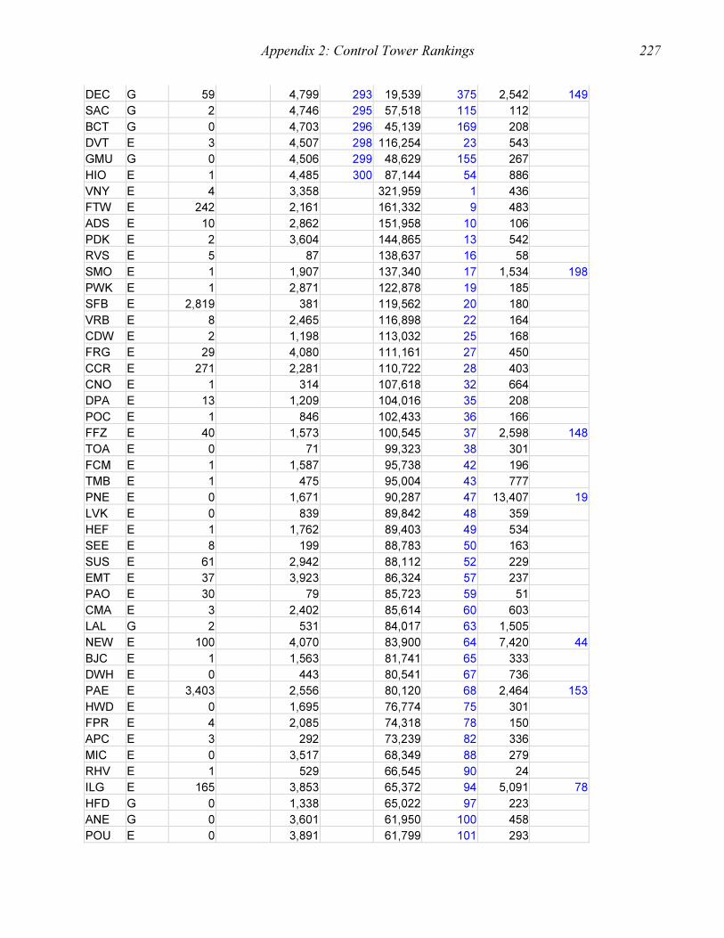
Appendix 2: Control Tower Rankings 227
DEC G 59 4,799 293 19,539 375 2,542 149
SAC G 2 4,746 295 57,518 115 112
BCT G 0 4,703 296 45,139 169 208
DVT E 3 4,507 298 116,254 23 543
GMU G 0 4,506 299 48,629 155 267
HIO E 1 4,485 300 87,144 54 886
VNY E 4 3,358 321,959 1 436
FTW E 242 2,161 161,332 9 483
ADS E 10 2,862 151,958 10 106
PDK E 2 3,604 144,865 13 542
RVS E 5 87 138,637 16 58
SMO E 1 1,907 137,340 17 1,534 198
PWK E 1 2,871 122,878 19 185
SFB E 2,819 381 119,562 20 180
VRB E 8 2,465 116,898 22 164
CDW E 2 1,198 113,032 25 168
FRG E 29 4,080 111,161 27 450
CCR E 271 2,281 110,722 28 403
CNO E 1 314 107,618 32 664
DPA E 13 1,209 104,016 35 208
POC E 1 846 102,433 36 166
FFZ E 40 1,573 100,545 37 2,598 148
TOA E 0 71 99,323 38 301
FCM E 1 1,587 95,738 42 196
TMB E 1 475 95,004 43 777
PNE E 0 1,671 90,287 47 13,407 19
LVK E 0 839 89,842 48 359
HEF E 1 1,762 89,403 49 534
SEE E 8 199 88,783 50 163
SUS E 61 2,942 88,112 52 229
EMT E 37 3,923 86,324 57 237
PAO E 30 79 85,723 59 51
CMA E 3 2,402 85,614 60 603
LAL G 2 531 84,017 63 1,505
NEW E 100 4,070 83,900 64 7,420 44
BJC E 1 1,563 81,741 65 333
DWH E 0 443 80,541 67 736
PAE E 3,403 2,556 80,120 68 2,464 153
HWD E 0 1,695 76,774 75 301
FPR E 4 2,085 74,318 78 150
APC E 3 292 73,239 82 336
MIC E 0 3,517 68,349 88 279
RHV E 1 529 66,545 90 24
ILG E 165 3,853 65,372 94 5,091 78
HFD G 0 1,338 65,022 97 223
ANE G 0 3,601 61,950 100 458
POU E 0 3,891 61,799 101 293
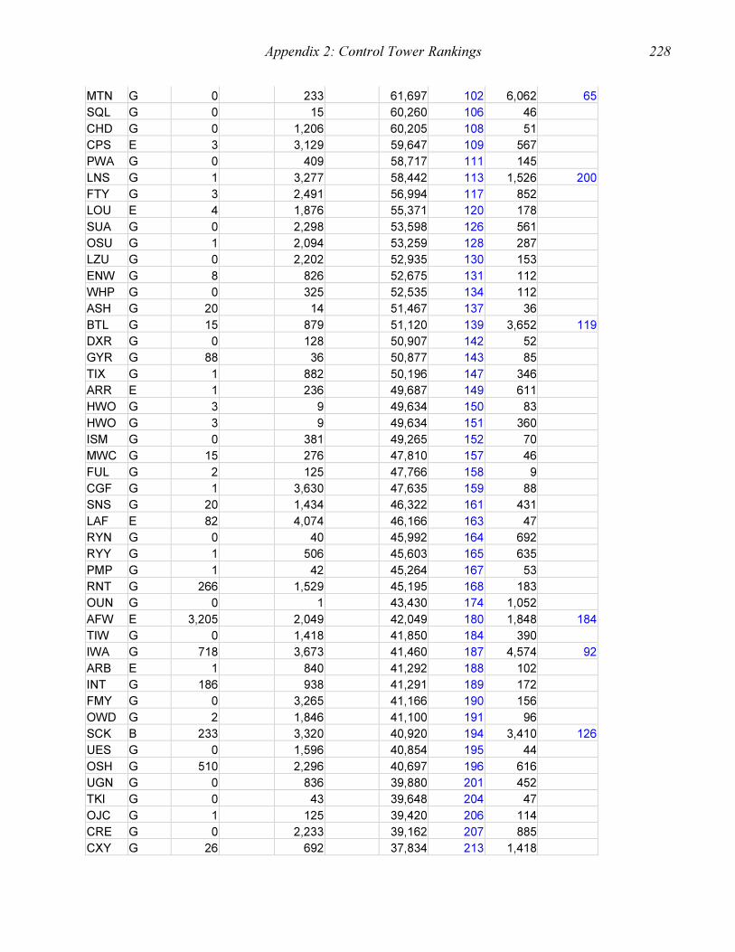
Appendix 2: Control Tower Rankings 228
MTN G 0 233 61,697 102 6,062 65
SQL G 0 15 60,260 106 46
CHD G 0 1,206 60,205 108 51
CPS E 3 3,129 59,647 109 567
PWA G 0 409 58,717 111 145
LNS G 1 3,277 58,442 113 1,526 200
FTY G 3 2,491 56,994 117 852
LOU E 4 1,876 55,371 120 178
SUA G 0 2,298 53,598 126 561
OSU G 1 2,094 53,259 128 287
LZU G 0 2,202 52,935 130 153
ENW G 8 826 52,675 131 112
WHP G 0 325 52,535 134 112
ASH G 20 14 51,467 137 36
BTL G 15 879 51,120 139 3,652 119
DXR G 0 128 50,907 142 52
GYR G 88 36 50,877 143 85
TIX G 1 882 50,196 147 346
ARR E 1 236 49,687 149 611
HWO G 3 9 49,634 150 83
HWO G 3 9 49,634 151 360
ISM G 0 381 49,265 152 70
MWC G 15 276 47,810 157 46
FUL G 2 125 47,766 158 9
CGF G 1 3,630 47,635 159 88
SNS G 20 1,434 46,322 161 431
LAF E 82 4,074 46,166 163 47
RYN G 0 40 45,992 164 692
RYY G 1 506 45,603 165 635
PMP G 1 42 45,264 167 53
RNT G 266 1,529 45,195 168 183
OUN G 0 1 43,430 174 1,052
AFW E 3,205 2,049 42,049 180 1,848 184
TIW G 0 1,418 41,850 184 390
IWA G 718 3,673 41,460 187 4,574 92
ARB E 1 840 41,292 188 102
INT G 186 938 41,291 189 172
FMY G 0 3,265 41,166 190 156
OWD G 2 1,846 41,100 191 96
SCK B 233 3,320 40,920 194 3,410 126
UES G 0 1,596 40,854 195 44
OSH G 510 2,296 40,697 196 616
UGN G 0 836 39,880 201 452
TKI G 0 43 39,648 204 47
OJC G 1 125 39,420 206 114
CRE G 0 2,233 39,162 207 885
CXY G 26 692 37,834 213 1,418
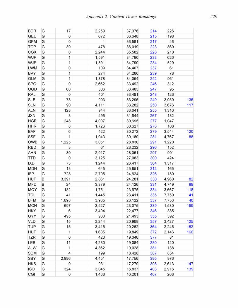
Appendix 2: Control Tower Rankings 229
BDR G 17 2,259 37,376 214 226
GEU G 0 672 36,648 215 198
GPM G 0 1 36,561 217 46
TOP G 39 478 36,019 223 869
CGX G 0 2,244 35,582 228 210
WJF G 1 1,591 34,790 233 626
WJF G 1 1,591 34,790 234 529
LWM G 0 109 34,407 237 61
BVY G 1 274 34,280 239 78
OLM G 1 1,878 34,054 242 961
SPG G 0 2,662 33,492 246 312
OGD G 60 306 33,485 247 95
RAL G 0 401 33,481 248 126
SLE G 73 993 33,296 249 3,059 135
SLN G 90 4,111 33,282 250 3,676 117
ALN G 128 944 33,041 255 1,316
JXN G 3 495 31,644 267 182
HGR G 248 4,007 30,695 277 1,047
HHR G 8 1,726 30,627 278 108
BAF G 6 422 30,272 279 3,544 120
SSF G 1 1,043 30,180 281 4,767 88
OWB G 1,225 3,051 28,830 291 1,220
RBD G 3 61 28,232 296 152
AHN G 30 2,917 28,051 297 901
TTD G 0 3,125 27,083 300 424
IXD G 73 1,244 26,417 304 1,317
MDH G 13 645 25,851 312 165
IFP G 728 2,705 24,624 326 180
HUF B 3,391 2,861 24,281 330 4,960 82
MFD B 24 3,379 24,126 331 4,749 89
MQY G 182 1,751 23,675 334 3,667 118
TCL G 41 1,445 23,411 335 7,750 41
BFM G 1,698 3,935 23,122 337 7,753 40
MCN G 697 3,527 23,075 339 1,530 199
HKY G 6 3,404 22,477 346 385
GYY G 495 930 21,493 355 392
VLD G 15 3,244 20,968 357 3,427 125
TUP G 15 3,415 20,262 364 2,245 162
HUT G 1 1,685 19,849 372 2,146 166
TZR G 0 420 19,346 377 81
LEB G 11 4,280 19,084 380 120
ALW G 1 4,362 19,028 381 138
SDM G 4 199 18,428 387 854
SBY G 2,896 4,451 17,756 395 976
HKS G 0 931 17,279 398 2,613 147
ISO G 324 3,045 16,837 403 2,916 139
CGI G 0 1,488 16,201 407 268
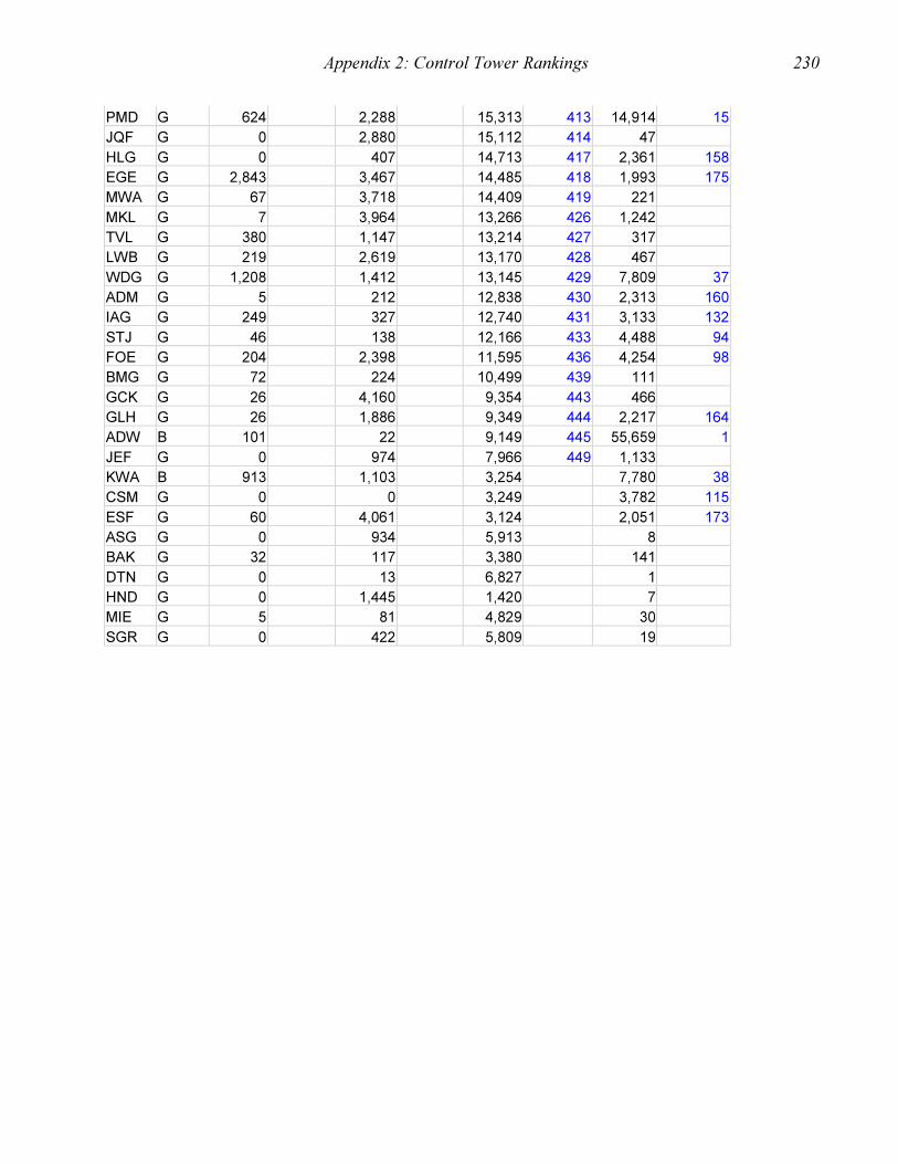
Appendix 2: Control Tower Rankings 230
PMD G 624 2,288 15,313 413 14,914 15
JQF G 0 2,880 15,112 414 47
HLG G 0 407 14,713 417 2,361 158
EGE G 2,843 3,467 14,485 418 1,993 175
MWA G 67 3,718 14,409 419 221
MKL G 7 3,964 13,266 426 1,242
TVL G 380 1,147 13,214 427 317
LWB G 219 2,619 13,170 428 467
WDG G 1,208 1,412 13,145 429 7,809 37
ADM G 5 212 12,838 430 2,313 160
IAG G 249 327 12,740 431 3,133 132
STJ G 46 138 12,166 433 4,488 94
FOE G 204 2,398 11,595 436 4,254 98
BMG G 72 224 10,499 439 111
GCK G 26 4,160 9,354 443 466
GLH G 26 1,886 9,349 444 2,217 164
ADW B 101 22 9,149 445 55,659 1
JEF G 0 974 7,966 449 1,133
KWA B 913 1,103 3,254 7,780 38
CSM G 0 0 3,249 3,782 115
ESF G 60 4,061 3,124 2,051 173
ASG G 0 934 5,913 8
BAK G 32 117 3,380 141
DTN G 0 13 6,827 1
HND G 0 1,445 1,420 7
MIE G 5 81 4,829 30
SGR G 0 422 5,809 19

231
Vita
James J. Galvin Jr. is currently serving as a Lieutenant Colonel in the United States
Army. After receiving the Ph.D. degree in Industrial and Systems Engineering from Virginia
Tech, he will serve as an Operations Research Analyst to assist in the large-scale organizational
transformation of the US Army. Lieutenant Colonel Galvin received a BS degree in Mechanical
Engineering from the United States Military Academy in 1983 and the MS degree in Operations
Research and Systems Analysis from the Naval Postgraduate School in 1991.