Contents lists available at ScienceDirect

Urban Climate

journal homepage: www.elsevier.com/locate/uclim

Air pollution knowledge assessments (APnA) for 20 Indian cities

Sarath K. Guttikundaa,b,⁎, Nishadh K.A.b, Puja Jawaharb

aDivision of Atmospheric Sciences, Desert Research Institute, Reno, USAbUrban Emissions, New Delhi, India

A R T I C L E I N F O

Keywords:PM2.5

Particulate pollutionIndiaEmissions inventoryDispersion modelingWRF-CAMx

Source apportionment

A B S T R A C T

Delhi, with a population of 22 million (1.6% of national total) is one of the most polluted capitalcities in the world. Nearly 50% of the published literature in India focus on air pollution in Delhi.However, air pollution impacts are not limited only to the capital city. Yet, there is little in-formation and attempt to quantify these impacts for Tier 1 and 2 cities, even though they accountfor> 30% of India's population. To remedy this vacuum of information, the Air Pollutionknowledge Assessments (APnA) city program deliberately focuses on 20 Indian cities, other thanDelhi. We established baseline multi-pollutant high-resolution emissions inventory, after col-lating information from multiple resources detailed in this paper, which was used to estimatespatial concentrations of key pollutants across city's urban airshed using WRF-CAMx chemicaltransport modeling system. The inventory includes anthropogenic sources, such as transport(road, rail, ship, and aviation), large scale power generation (from coal, diesel, and gas powerplants), small scale power generation (from diesel generator sets for household use, commercialuse, and agricultural water pumping), small and medium scale industries, dust (road resuspen-sion and construction), domestic (cooking, heating, and lighting), open waste burning, and openfires and non-anthropogenic sources, such as sea salt, dust storms, biogenic, and lightning. Theemissions inventory is currently in use for 3-day advance air quality forecasting for public releaseon an on-going basis. Using meteorological parameters and big data like gridded speed mapsfrom google, the emissions inventory is dynamically updated. The results from this research willbe valuable to local and national policy makers - especially the information on source con-tributions to air pollution.

1. Introduction

That air pollution is a serious environmental health issue in India is not under debate. The global burden of disease assessmentsestimated 0.74 million and 1.1 million premature deaths in 1990 and 2016 due to outdoor PM2.5 and ozone pollution and 0.99million and 0.78 million premature deaths in 1990 and 2016 due to household (indoor) PM2.5 pollution (GBD, 2018). In the mon-itoring database released by the World Health Organization (WHO) in April 2018 covering 100 countries for the period of 2011 and2016, India has 14 of the top 15 cities with the worst PM2.5 pollution. Among megacities of the world, Delhi tops the list for PM10

pollution (WHO, 2018). What is unclear however is the extent of the problem in India. The maps in Fig. 1 compares surface PM2.5

pollution levels for 1998, 2010, and 2016 extracted from Van Donkelaar et al. (2016). These data were produced using a combinationof satellite observations, global chemical transport model using global emission inventories, and available ground-based measure-ments. Of the 640 districts in India (as per 2011 Census), 27% exceed the current annual standard of 40 μg/m3 in 1998, 45% and 63%

https://doi.org/10.1016/j.uclim.2018.11.005Received 3 August 2018; Received in revised form 9 November 2018; Accepted 19 November 2018

⁎ Corresponding author at: Division of Atmospheric Sciences, Desert Research Institute, Reno, USA.E-mail address: sarath-guttikunda@uiowa.edu (S.K. Guttikunda).

Urban Climate 27 (2019) 124–141

2212-0955/ © 2018 Published by Elsevier B.V.

T

Fig.

1.Su

rfacean

nual

averag

ePM

2.5co

ncen

trations

(inμg

/m3)for19

98,2

010,

and20

16,b

ased

onsatellite

observations,g

loba

lche

mical

tran

sportm

odel

simulations

usingglob

alem

ission

inve

ntories,

andav

ailablegrou

nd-based

measuremen

ts(V

anDon

kelaar

etal.,20

16).

S.K. Guttikunda et al. Urban Climate 27 (2019) 124–141

125

exceed the same in 2010 and 2016. 99.5% of them exceed the WHO guideline of 10 μg/m3 in 2016.With urbanization, domestic migration is not only increasing population in the major metropolitan cities, but also in medium and

small cities. These towns are adjusting their infrastructure needs, such as transport and waste management, to accommodate thegrowing population and economy. To take the air pollution policy debate further at the national scale, we need to move beyondanecdotal evidence, quantify and spatially map out pollution, and assess the impact of sources at the local scale (Guttikunda et al.,2014).

Big cities have some published studies that quantified source contributions, which led to some policy discussion (Pant andHarrison, 2012). The Central Pollution Control Board (CPCB, New Delhi, India) conducted a source apportionment study for six cities– Bengaluru, Chennai, Delhi, Kanpur, Mumbai, and Pune in 2006 (CPCB, 2011). It has been at least 12 years since CPCB has con-ducted any other source apportionment studies. There is very little information for other cities on ambient monitoring and sourcecontributions. Of the number of scientific studies conducted to identify the sources of PM2.5 and PM10 pollution via chemical analysisand receptor modeling since 2000, 70% repeatedly covered Delhi, Mumbai, Kolkata, Chennai, Hyderabad, and Agra (Guttikundaet al., 2014). We distilled relevant journal articles by conducting a full search on the SCOPUS database (title, abstract, and keywords)for all articles published between 2000 and 2017 for 50 Indian cities. This was done to get an idea of the state of research on topicsrelated to air pollution - emission inventories, industrial studies, dispersion modeling, source apportionment, emission factors, andambient monitoring. Accordingly, we collected 543 papers that mentioned at least one Indian city. Unsurprisingly, Delhi is the moststudied city in India with 283 hits (> 50% of the total). Mumbai, the commercial capital of India and Kolkata, tied for a distantsecond with 35 hits each (Fig. 2). The trend in the number of publications is also an indication of the importance given to the airpollution problem in Delhi by the researchers, media, and national/international organizations.

Designing an effective air quality management plan for a city requires robust data on the sources of air pollution. The AirPollution knowledge Assessments (APnA) city program is an attempt to fill the vacuum of information and by creating a baseline ofair pollution related information for Indian cities, a necessary starting point for the policy makers, academic researchers, and citizensto chart out strategies for better air quality. We believe that establishing the baseline or quantifying the extent of the problem in citiesother than the metropolitan cities is the starting point for change.

In this paper, we present our work on building these baselines for 20 Indian cities as (a) review of city characteristics such asambient air quality, urban growth, census fields, geography, and meteorology (b) multi-pollutant emission inventory at 1-km re-solution for the city airsheds and (c) WRF-CAMx chemical transport modeling to study trends and estimate source contributions toPM2.5 and PM10 pollution.

2. City airsheds

For 20 Indian cities, we collated city geography and related characteristics as listed in Table 1. The list includes 2 megacities(Bengaluru and Chennai) with population above 10 million; 4 cities with population between 5 and 10 million (Chandigarh, Kanpur,Patna and Pune); 12 cities with population between 2 and 5 million; 2 cities (Dehradun and Ranchi) with population between 1 and 2million. This list covers 13 states and 1 union territory (Chandigarh). These 20 cities host 90 million inhabitants (approximately 7.5%of national total) over an airshed of 44,000 sq.km (approximately 1.3% of national total). Table 2 catalogues a brief description of theselected cities.

The Supplementary resources include the Google KML files of individual city airsheds. For each city, on average 25% of airshedsarea is designated as urban and extends beyond the political boundaries to include sources that may contribute to air pollution in themain city. 7 of 20 cities are on the Indo-Gangetic plain, the most polluted region in India (Fig. 1); 2 coastal cities with big commercialports (Chennai and Kochi); 1 city in the hills (Dehradun); 14 North Indian cities and 6 South Indian cities.

For each airshed, we extracted built up area from Pesaresi et al. (2016) for 1975, 1990, 2000, and 2014 (Table 1). Fig. 3(a) offers acomparison of the built-up areas between 1990 and 2014 for 4 cities – Agra, Bengaluru, Chennai, and Patna. Remaining figures are

Fig. 2. Number of journal articles published between 2000 and 2017 (from SCOPUS search) with some reference to air pollution research in anIndian city.

S.K. Guttikunda et al. Urban Climate 27 (2019) 124–141

126

included in the Supplementary. Built up area on average increased by 200% between 1975 and 2000 and by 40% between 2000 and2014. Chandigarh, one of the original planned cities, showed the least increase in built-up area, while cities with the largest per-centage change are Bhubaneswar, Indore, Jaipur, Kanpur, and Pune.

3. Air quality monitoring

The CPCB and the State Pollution Control Boards (SPCBs) maintain and operate the national ambient monitoring programme(NAMP). This is the only official ambient monitoring database available in India since 1990. The monitoring network is slowlyexpanding. In 2015, there were 206 manual monitoring stations in 46 cities. As of May 2018, there are 700 manual stations and 117continuous stations (33 stations are operating in Delhi). In September 2017, there were 74 continuous stations in operation – a 50%increase over 6months. The continuous ambient monitoring stations report pollution levels for all the criteria pollutants every15min. This data is available in real time on CPCB's website.

The manual stations measure PM2.5, PM10, SO2, and NO2 and the procedure includes manually changing and collecting samples.While PM2.5 as a criteria pollutant was introduced in 2009, it was only added as a pollutant to be measured at the manual stations in2016. The Supplementary includes all available manual monitoring network data for the years between 2011 and 2015. For themanual stations, details on time of sample collection and time of filter change are unknown. Standard protocol suggests that at least100 samples per station are required. In 2016, number of collection days for all stations averaged 94.2 for PM10, 93.9 for SO2, 94.6 forNO2, and 71.3 for PM2.5.

The WHO (2018) report utilized the data from both manual and continuous networks. Table 3 lists a summary of the data used inthe WHO report. Of the 14 Indian cities in the top 15 most polluted cities, except for Delhi, Lucknow, and Agra, the remaining 11cities – Kanpur, Faridabad, Varanasi, Gaya, Patna, Muzaffarpur, Srinagar, Gurgaon, Jaipur, Patiala, and Jodhpur, have one mon-itoring station each. A sample of one is not enough to know the true spatial and temporal trend of air pollution in any city.

Including Delhi, all the cities are operating less than the required number of monitoring stations to truly represent the mix ofsources and activities in the city. Unlike cities in Europe and the United States, where vehicle exhaust is the main source of pollution,the range of sources in Indian cities is wide - from large and small industries to vehicle exhaust to road dust to biomass burning everyday for cooking and heating. Using the CPCB's thumb rule (CPCB, 2003), which considers the total population of an airshed and themix of activities, we estimate a need for 4000 continuous monitoring stations in India – 2800 in the urban areas and 1200 in the ruralareas, to represent a population of 1.3 billion. These details at the state and the district level are presented in the Supplementary. Forexample, Uttar Pradesh with a population of over 200 million requires 558 stations and Delhi with a population of over 20 millionrequires 77.

Table 4 is a summary of the available ambient monitoring data and the number of manual and continuous monitoring stationsoperational in 20 Indian cities from this study. Air monitoring capacity is low in all the cities. As of May 2018, 6 of 20 cities do nothave any continuous monitoring stations; 11 cities have only one continuous monitoring station. Bengaluru added 5 new continuous

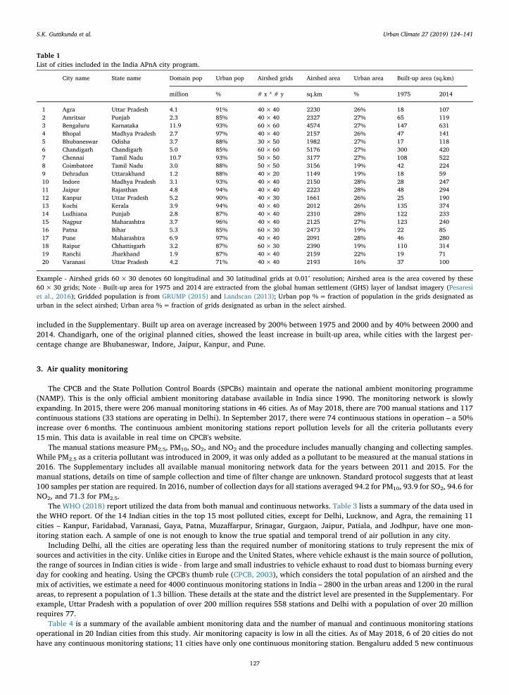
Table 1List of cities included in the India APnA city program.

City name State name Domain pop Urban pop Airshed grids Airshed area Urban area Built-up area (sq.km)

million % # x * # y sq.km % 1975 2014

1 Agra Uttar Pradesh 4.1 91% 40×40 2230 26% 18 1072 Amritsar Punjab 2.3 85% 40×40 2327 27% 65 1193 Bengaluru Karnataka 11.9 93% 60×60 4574 27% 147 6314 Bhopal Madhya Pradesh 2.7 97% 40×40 2157 26% 47 1415 Bhubaneswar Odisha 3.7 88% 30×50 1982 27% 17 1186 Chandigarh Chandigarh 5.0 85% 60×60 5176 27% 300 4207 Chennai Tamil Nadu 10.7 93% 50×50 3177 27% 108 5228 Coimbatore Tamil Nadu 3.0 88% 50×50 3156 19% 42 2249 Dehradun Uttarakhand 1.2 88% 40×20 1149 19% 18 5910 Indore Madhya Pradesh 3.1 93% 40×40 2150 28% 28 24711 Jaipur Rajasthan 4.8 94% 40×40 2223 28% 48 29412 Kanpur Uttar Pradesh 5.2 90% 40×30 1661 26% 25 19013 Kochi Kerala 3.9 94% 40×40 2012 26% 135 37414 Ludhiana Punjab 2.8 87% 40×40 2310 28% 122 23315 Nagpur Maharashtra 3.7 96% 40×40 2125 27% 123 24016 Patna Bihar 5.3 85% 60×30 2473 19% 22 8517 Pune Maharashtra 6.9 97% 40×40 2091 28% 46 28018 Raipur Chhattisgarh 3.2 87% 60×30 2390 19% 110 31419 Ranchi Jharkhand 1.9 87% 40×40 2159 22% 19 7120 Varanasi Uttar Pradesh 4.2 71% 40×40 2193 16% 37 100

Example - Airshed grids 60× 30 denotes 60 longitudinal and 30 latitudinal grids at 0.01° resolution; Airshed area is the area covered by these60× 30 grids; Note - Built-up area for 1975 and 2014 are extracted from the global human settlement (GHS) layer of landsat imagery (Pesaresiet al., 2016); Gridded population is from GRUMP (2015) and Landscan (2013); Urban pop %= fraction of population in the grids designated asurban in the select airshed; Urban area %= fraction of grids designated as urban in the select airshed.

S.K. Guttikunda et al. Urban Climate 27 (2019) 124–141

127

Table 2General description of the cities included in the India APnA city program.

City Description

1 Agra On the banks of river Yamuna, the city is known for the Taj Mahal – a UNESCO World Heritage site, which attracts at least 8 milliontourists every year. Agra's economy is made up of a thriving small-scale industry sector connected to handicrafts, leather goods, and ironfoundries, tourism, and agriculture. The delicate inlay and carving work in white marble of the Taj Mahal started getting affected by therising air pollution levels. In 2000, the Supreme Court mandated a 50-km safe-zone known as the “Taj Trapezium Zone” (TTZ) – whichwill be free of polluting industry and fueled vehicles. This has had scant impact on the pollution levels in the city, as Agra ranked 4th mostpolluted in 2016.

2 Amritsar City is home to the Golden Temple (the spiritual center for the Sikh community) and lies on the Grand Trunk road (GT Road) from Delhi toLahore in Pakistan. The temple visitors frequently take inter-city buses contributing to the day to day commercial and transportationactivities in the city. Within the city, majority of the short trips are covered by rickshaws, auto rickshaws, and taxis. Amritsar's economy ismade up of tourism, carpets and fabrics, farm produce, handicrafts, service trades, and light engineering. Coupled with small and heavyvehicles plying along the GT Road, vehicle exhaust and road resuspended dust has become a major source of air pollution in the city,especially due to 50,000 unregistered autorickshaws and double that of the registered ones. A majority of these use petrol mixed withkerosene.

3 Bengaluru Bengaluru (formerly Bangalore), the capital of Karnataka was a pioneer in that it was one of the first information technology (IT) hubs ofIndia. What was once a laid-back retiree town, is now a bustling metropolis with 10+ million inhabitants. The population grewexponentially from 1980s with several companies, especially IT industry, establishing base in the city, creating higher demand fortransport and construction. The unplanned growth in the city boosted the infrastructure activities that the municipality attempted to easeby constructing a flyover system and by imposing one-way traffic systems, which were unable to adequately address the on-road issuesand associated increase in air pollution. As the demand for housing has grown, the city finds itself spreading beyond its erstwhileboundaries to accommodate it.

4 Bhopal Bhopal, the capital of Madhya Pradesh, has been selected under National Smart Cities program's first round for integrated urbandevelopment. The old city of Bhopal is home for small and medium industries covering electrical goods, medicinal products, cotton,chemicals, jewelry, flour milling, cloth weaving, painting, matches manufacturing, wax manufacturing, and sporting equipment. It alsohouses the Bharath Heavy Electricals Limited (BHEL), which is one of the largest engineering companies in India that manufactures coal-fired power plant boilers (among many other heavy machinery). Mandideep, another industrial suburb to the south of the city, is thelargest industrial area in Madhya Pradesh. Bhopal is also synonymous with the Union Carbide Bhopal Disaster in the early 1980s.

5 Bhubaneswar Cuttack was replaced by Bhubaneswar as the capital of Odisha (formerly Orissa) in 1949 and is one of the first planned cities in India,along with Jamshedpur and Chandigarh. Together they are referred to as the twin cities of Odisha. The city lies on the banks of Mahanadiriver and between the naturally rich plains of Daya river and Kuakhai Rivers. As a tier-2 city, it is emerging as a center for education andIT. With increasing population, construction activity, and transport demand and limited waste management options, air pollution isreaching critical levels, even in the summer months.

6 Chandigarh Chandigarh is a union territory that serves as the capital for the states of Haryana (on the east) and Punjab (on the north, west and south).Chandigarh airshed includes Patiala and Ambala, all within a 30 km radius of each other. Chandigarh, was one of the first planned citiesin India and is known for its urban design, by Swiss architect Lr Corbusier, and sometimes referred to as “Pensioner's Paradise”. There are15 medium to large industries and over 2500 smaller units manufacturing paper, basic metals and alloys, machinery, food products,sanitary ware, auto parts, machine tools, pharmaceuticals, and electrical appliances.

7 Chennai As the capital city of Tamil Nadu, Chennai is one of four metropolitan cities of India with 10+ million inhabitants. With its proximity tothe Bay of Bengal and thus access to markets in East Asia, it is also an important port city. Apart from trade and shipping, the automobileindustry (30% of India's auto industry), chemical and petrochemical industry, software services, medical care, and manufacturing formthe foundation of the economic base for Chennai. The Ennore Port, the first major corporate port with an annual capacity of 30 milliontons of cargo in 2012–2013, handles coal (most of the supply is for the two thermal power plants with dedicated feeder lines running fromthe ports), iron ore, oil, and commercial commodities.

8 Coimbatore After Chennai, Coimbatore is the second largest city in Tamil Nadu, located on Noyyal river bank and surrounded by the Western Ghats,houses > 25,000 small, medium and large industries covering textile and cotton industry, manufacturing, poultry farming, education, IT,and health care.

9 Dehradun Dehradun, is the capital of Uttarakhand, carved out of the state of Uttar Pradesh in 2000. The city capital lies in the Doon Valley, in thefoothills of the Himalayas, between the river Ganges on the east and the river Yamuna on the west. The city was developed as a getawayfrom the hot summers of the plains and hosts several institutions such as the Indian Military Academy (IMA), ITBP Academy, IndiraGandhi National Forest Academy (IGNFA), Zoological Survey of India (ZSI), Forest Research Institute (FRI) among several others.Construction and transport are the fastest growing sectors in the region. The geographical and meteorological conditions do not allow foreasy dispersal of emissions.

10 Indore Indore is 200 km from Bhopal, is the largest city and the commercial center in the state of Madhya Pradesh and part of the 100 smart citiesprogram in India. A network of national and state highways through the city (NH3 to Agra and Bombay; NH59 to Ahmedabad and Betul;SH27 to Burhanpur; and SH34 to Jhansi) made it an important transport and logistics hub in the country. Major industrial areas are inPithampur and Sanwer special economic zones focusing on soybean processing, automobile, IT, and pharmaceuticals.

11 Jaipur As the state capital of Rajasthan, Jaipur is located 260 km from New Delhi and forms a part of a popular tourist circuit with Agra(240 km). Jaipur also serves as a gateway to other tourist destinations in Rajasthan such as Jodhpur, Jaisalmer, Udaipur, and Mount Abu.City is an educational and administrative center and its economy is fueled by tourism, gemstone cutting for jewelry, luxury textiles, andIT. During winter months, flights towards New Delhi airport are often diverted to Jaipur airport under foggy conditions. Another tellingstatistic that illustrates the level of traffic congestion in Jaipur is that 60% of the city roads are used for parking – the highest in any city inIndia (CSE, 2017).

12 Kanpur Kanpur is one of the largest industrial towns in North India, on the Indo-Gangetic plain, and the largest city in the state of Uttar Pradesh.Kanpur supports the largest textile and leather processing sectors in the region. Kanpur briefly attempted to put in place a public-privatepartnership system for solid waste management, which after failing led to one of the major causes of air, water, and waste managementissues in the city. In 2011, CPCB's assessment of air pollution in six cities (Delhi, Mumbai, Kanpur, Pune, Chennai and Bangalore) reportedthat air pollution sources in Kanpur are industries (biggest cause) followed by open waste burning, vehicles, road dust, and domesticcooking (CPCB, 2011).

13 Kochi

(continued on next page)

S.K. Guttikunda et al. Urban Climate 27 (2019) 124–141

128

monitoring stations in 2018, bringing their total to 10, which is 25% of the recommended capacity to represent approximately 11.9million inhabitants.

All cities exceed the annual PM10 standard of 60 μg/m3. Major sources of PM10 include combustion of coal, kerosene, petrol,diesel, biomass, cow dung, and waste as well as dust. Coimbatore reported just above the standard. 6 cities - Agra, Bengaluru, Jaipur,Kanpur, Ludhiana, and Raipur, recorded 4–6 times the annual standard. These are among the fastest growing Indian cities, tradi-tionally known to be dusty due to a lot of construction activities and dust on the roads which is resuspended when vehicles pass.

All cities comply with the annual SO2 standard of 50 μg/m3. Major sources of SO2 include combustion of coal and diesel.Bengaluru, Chennai, and Pune (most populated of the 20) recorded the highest SO2 concentrations, indicating higher consumption ofdiesel in personal vehicles, freight vehicles, and diesel generator sets.

9 of 20 cities exceed the annual NO2 standard of 40 μg/m3. Major sources of NO2 include combustion of petrol, diesel, and gas(i.e., transport related emissions) and large industries. Bengaluru, Chennai, Jaipur, Nagpur, Kanpur, and Pune record the highestconcentrations.

Satellite observations coupled with global model simulations provide a useful baseline to monitor progress and validation (vanDonkelaar et al., 2016). Table 3 lists data extracted for years 1998 and 2016. Refer to the Supplementary for data for all years inbetween and all 640 districts. These methodologies are an integral part of the global burden of disease estimates for outdoor andindoor air pollution (Brauer et al., 2016; GBD, 2018; Shaddick et al., 2018) and the premature death due to outdoor PM2.5 estimatespublished by WHO (WHO, 2016). The model estimates underrepresent the pollution levels due to a mix of unknowns, such as modelgrid resolution, uncertainties in the emission inventories, lack of enough ground-based measurements to corelate with the satelliteobservations. Of the 20, only 5 cities show concentrations under the national ambient standard of 40 μg/m3 – Chennai and Kochi arecoastal cities and Bhubaneswar close to the coast, with the advantage of land-sea breeze that disperses most of the emissions from theindustries, vehicles, and ports; Bengaluru and Coimbatore, also in South India have the advantage of strong winds to disperse most ofthe emissions. North India is landlocked, has a greater population density and a higher concentration of settlements. As a result, alongwith meteorological factors, there is an increase of 50–100% in their ambient PM2.5 pollution levels between 1998 and 2016.

Table 2 (continued)

City Description

Kochi in the state of Kerala is an important port town and houses the Southern Naval Command of the armed forces, the largestinternational container trans-shipment terminal in India (the Cochin shipyard), and the offshore mooring of the Bharath PetroleumCorporation Limited (BPCL). It is also an important chemical industrial and manufacturing hub and an emerging IT center in Kerala.

14 Ludhiana Ludhiana is an agricultural and industrial town in Punjab housing several small scale industrial units producing auto parts, appliances,machine parts, and apparel. The city has been on the most polluted list, drawn by WHO for multiple years. The distributed industries,generator use, agriculture burning, adulterated fuel for three-wheelers and adverse meteorological conditions (in the winter months), andopen field burning (post-harvest season before the winter months) are responsible for its bad air quality.

15 Nagpur Nagpur holds the distinction of being the geographical center of the Indian peninsula. Nagpur lies on the Deccan plateau and is the 3rdlargest city and a major commercial and political center of the state of Maharashtra. Agriculture (in particular oranges and ayurvedicmedicine processing) forms a large share of its economy, along with IT, manufacturing, transport systems, and mining. Due to itsproximity to the coal belt in Central India, power generation from coal is large (47% of state's power is generated around Nagpur). Thegovernment is investing in Nagpur's infrastructure development to make it a freight movement hub.

16 Patna As the state capital of Bihar, Patna with 72 wards is the largest in the state, located on the banks of rich Indo-Gangetic plain, and is amongthe states with the highest population density. The city economics is supported by agricultural activities (> 30% is rice), small scalemanufacturing industries (including brick kilns, pulses, shoes, scooters, masur, chasra, electrical goods, and cotton yarn), and powergeneration (3000MW power plant 100 km west of the city).

17 Pune Once referred to as a city for students and retirees, Pune has now established manufacturing, glass, sugar, and metal forging industries,and more recently IT and auto industry. The Hinjewadi IT Park (located west of the Pimpri Chinchwad satellite city) is a project started byMaharashtra Industrial Development Corporation and Magarpatta city under a special economic zone scheme to the east has over 20,000inhabitants, mostly working on IT. Construction of townships and developments mean that raw material from stone quarries, river sandand bricks are in constant demand. Fugitive dust emissions from the quarrying process, use of diesel for power generation in thecommercial and industrial sectors, vehicle exhaust of heavy duty trucks moving in and out of the quarries, brick kiln clusters, andmanufacturing industries is on the rise.

18 Raipur In Chhattisgarh, Raipur-Durg-Bhilai (RDB) tri-city area hosts the new administrative capital of the state, interconnected by an expresswayforming the industrial corridor, and located on the banks of the Mahanadi River. RDB is the largest steel manufacturing hub in India and ishome to several foundries, metal-alloy plants, steel casting and rolling, sponge iron plants, cement production, and a large chemical(formalin) manufacturing plant. Bhilai Steel plant is the largest integrated steel plant in India. Most of the electricity generation at thepower and the steel plants is coal-based. While Durg-Bhilai are largely industrial, Raipur has emerged as the commercial hub. Naya Raipur(New Raipur) is a satellite city located 17 km away from Raipur covering 8000 ha is expected to house 450,000 inhabitants.

19 Ranchi Ranchi is the state capital of Jharkhand (the state was formed in 2000) and is part of the smart cities program in India. Much of the city'seconomy is driven by processing industry based on resources from the forests of Jharkhand. These include timber, matches, rayon,medicinal plants and seeds. It is a relatively small city, but from the time the state was formed in 2000, the number of vehicles in the cityhas increased 20 times. With an increase in population – this erstwhile hill station is now dealing with haphazard construction andinsufficient systems for solid waste management leading to open burning.

20 Varanasi Formerly Banaras, Varanasi lies on the banks of the Ganges river in Uttar Pradesh and is center for pilgrimage and tourism in India (~3million domestic and 200,000 visitors annually). This puts a significant burden on city's solid waste management infrastructure, withmuch of the waste either burnt or dumped in landfills or in the river). City is famous for several handcrafted goods such as muslin and silkfabrics, perfumes, ivory works, and sculpture, diesel locomotive works, and Bharat Heavy Electricals Ltd.

S.K. Guttikunda et al. Urban Climate 27 (2019) 124–141

129

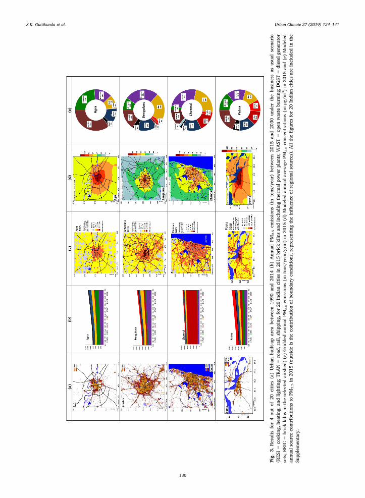
Fig.

3.Results

for4

outof

20cities

(a)Urban

built-up

area

betw

een

1990

and

2014

(b)Ann

ualPM

2.5

emission

s(in

tons/y

ear)

betw

een

2015

and

2030

unde

rthebu

sine

ssas

usua

lscen

ario

(RES

I=co

oking,

heating,

andlig

hting;

TRAN=

road

,rail,shipping

,for

20Indian

cities

in20

15brickkilnsan

dinclud

ingthermal

power

plan

ts;W

AST

=op

enwaste

burning;

DGST

=diesel

gene

rator

sets;B

RIC

=brickkilnsin

theselected

airshe

d)(c)Gridd

edan

nual

PM2.5em

ission

s(intons/y

ear/grid)in

2015

(d)Mod

eled

annu

alav

erag

ePM

2.5co

ncen

trations

(inμg

/m3)in

2015

and(e)Mod

eled

annu

alsource

contribu

tion

sto

PM2.5in

2015

(outside

istheco

ntribu

tion

ofbo

unda

ryco

nditions,rep

resentingtheinflue

nceof

region

alsources).A

llthefigu

resfor20

Indian

cities

areinclud

edin

the

Supp

lemen

tary.

S.K. Guttikunda et al. Urban Climate 27 (2019) 124–141

130

4. Urban emission inventories

4.1. Methods and data

We built an emissions inventory for each of the 20 cities for year 2015 for the following pollutants – particulate matter (PM) infour classes (a) PM10 (b) PM2.5 (c) black carbon (BC) and (d) organic carbon (OC), SO2, nitrogen oxides (NOx), carbon monoxide (CO),non-methane volatile organic compounds (NMVOCs), and carbon dioxide (CO2). We also projected the emission loads to year 2030under a business as usual scenario after accounting for policy interventions already under implementation (e.g. accelerated in-troduction of liquified petroleum gas (LPG) for cooking). The emissions inventory developed under the APnA programme is the firstof its kind for most of them. The main challenge is that useful and formatted data necessary to build an emissions inventory is hard tocome by. We thus accessed data from a wide array of sources for each sector.

We built the emissions inventory at a resolution of 0.01° (approximately 1-km). This includes anthropogenic sources, such astransport (road, rail, ship, and aviation), large scale power generation (from coal, diesel, and gas power plants), small scale powergeneration (from diesel generator sets for household use, commercial use, and agricultural water pumping), small and medium scaleindustries, dust (road resuspension and construction), domestic (cooking, heating, and lighting), open waste burning, and open firesand non-anthropogenic sources, such as (where relevant) sea salt, dust storms, biogenic, and lightning. Using geospatial platforms,the inventory is formatted such that it can be used for urban and regional chemical transport modeling.

We use the SIM-air (Simple Interactive Models for better air quality) family of tools to estimate total emissions. This is a functionof fuel burnt which is then converted to emission loads using relevant emission factors. We used the same methodology for similarprojects for 10 Indian cities – Pune, Chennai, Ahmedabad, Indore, Surat, Rajkot, Hyderabad, Chennai, Vishakhapatnam, and Delhi

Table 3Breakdown of the PM2.5 concentrations data presented in WHO (2018).

Number of cities with measured PM2.5 33

Number of cities with measured + converted PM2.5 135Average PM2.5 for cities with measured concentrations 84.2 ± 46.2 μg/m3

Average PM2.5 for cities with converted concentrations 53.5 ± 30.4 μg/m3

National annual ambient standard for PM2.5 40 μg/m3

World Health Organization annual guideline for PM2.5 10 μg/m3

Number of cities with 1 station only for PM2.5 measurements 23Number of cities with 1,2,3 stations for converted PM2.5 30,28,33Number of cities with 4+ stations for converted PM2.5 7Year of data reported for PM2.5 measurements (number of cities) 2016(33)Year of data reported for converted PM2.5 (number of cities) 2011 (1), 2012 (97), 2013 (1), 2014 (1), 2015 (2)

Table 4Number of operational stations (as of May 2018), number of minimum stations required, annual average PM2.5, PM10, SO2, and NO2 concentrations(in μg/m3), and modeled surface PM2.5 concentrations from Fig. 1, in the 20 cities under the APnA city program.

Monitoring stations 2011–2015 manual 2015–2017 continuous PM2.5 from Fig. 1

City name Man. Cont. Reco. PM10 NO2 SO2 PM2.5 1998 2016

1 Agra 6 1 23 362.2 ± 193.1 43.9 ± 22.1 9.3 ± 5.4 98.6 ± 86.1 77.1 116.92 Amritsar 3 1 18 195.6 ± 44.9 38.9 ± 7.6 13.8 ± 2.6 65.9 ± 64.8 41.5 79.13 Bengaluru 16 10 41 302.5 ± 208.0 69.2 ± 44.0 30.9 ± 23.5 32.3 ± 24.2 19.7 28.94 Bhopal 5 1 18 196.3 ± 117.3 23.2 ± 16.9 2.9 ± 2.5 47.8 ± 35.1 31.7 56.55 Bhubaneswar 5 0 22 128.0 ± 102.7 26.9 ± 17.2 3.0 ± 1.5 17.1 37.96 Chandigarh 5 1 27 226.9 ± 103.6 44.3 ± 32.4 4.0 ± 1.9 59.4 ± 62.7 44.8 78.77 Chennai 11 3 38 199.8 ± 101.5 65.5 ± 37.1 39.7 ± 31.8 47.7 ± 73.7 17.6 32.68 Coimbatore 3 0 19 62.5 ± 39.7 26.9 ± 15.3 4.0 ± 1.7 14.1 26.09 Dehradun 3 0 13 170.3 ± 53.8 26.3 ± 8.0 23.9 ± 7.3 53.5 87.410 Indore 3 1 20 139.2 ± 69.8 18.9 ± 3.9 11.3 ± 3.7 40.4 ± 23.1 27.7 46.111 Jaipur 6 3 26 313.9 ± 141.3 79.8 ± 25.3 14.5 ± 7.5 70.4 ± 76.8 43.1 68.312 Kanpur 8 1 27 421.1 ± 188.5 70.7 ± 32.0 14.0 ± 11.7 111.4 ± 79.7 69.7 106.613 Kochi 7 0 23 221.6 ± 167.0 38.4 ± 30.5 10.7 ± 10.6 13.9 26.114 Ludhiana 4 1 20 335.0 ± 149.6 48.0 ± 14.4 18.7 ± 6.0 74.4 ± 46.1 44.9 83.915 Nagpur 7 1 22 192.1 ± 112.5 64.7 ± 36.0 20.7 ± 18.8 53.9 ± 26.7 28.4 47.316 Patna 2 1 26 162.5 ± 91.7 33.0 ± 24.3 4.6 ± 5.0 121.3 ± 89.5 52.1 90.817 Pune 4 1 30 162.2 ± 104.3 82.5 ± 45.0 40.3 ± 20.9 43.1 ± 25.7 30.9 47.518 Raipur 2 0 19 275.2 ± 81.0 35.3 ± 13.3 12.9 ± 5.0 29.6 54.619 Ranchi 1 0 16 190.1 ± 52.3 35.1 ± 5.4 18.3 ± 2.0 32.5 55.620 Varanasi 2 1 23 139.3 ± 15.9 26.2 ± 6.7 18.4 ± 2.5 106.2 ± 83.4 51.7 94.0

Note: Man. = manually operated stations where filter papers are collected 2 times per week on average; Cont. = continuous ambient monitoringstations reporting data every 15min; Reco. = recommended number of continuous monitoring stations for the city.

S.K. Guttikunda et al. Urban Climate 27 (2019) 124–141

131

(Guttikunda and Jawahar, 2012; Guttikunda and Calori, 2013; Guttikunda and Kopakka, 2014; Guttikunda et al., 2014); nationaltransport sector (Guttikunda and Mohan, 2014); national power plant sector (Guttikunda and Jawahar, 2014); and Delhi transportsector (Goel and Guttikunda, 2015). We used multiple sources to collate a library of emission factors for transport, industrial, anddomestic sectors (CPCB, 2011; Pandey et al., 2014; Sadavarte and Venkataraman, 2014; IIASA, 2015; Goel and Guttikunda, 2015;Sakar et al., 2016). For this purpose, we documented and digitized information available from the annual reports, maps, and da-tabases such as census and ambient measurements. A copy of the India specific emission factors for all the sectors from IIASA (2015),by fuel and by activity, is available online (registration required).

Data to build the emissions inventory includes;

• Static Data - CPCB, state PCBs, Census Bureau, Niti Aayog, National Sample Survey Office (NSSO), Ministry of Road Transport andHighways (MoRTH), Society of Indian Automobiles Manufacturers (SIAM), Directorate general of Civil Aviation (DGCA), Ministryof Petroleum and Natural Gas (MoPNG), Ministry of Statistics and Program Implementation, Annual Survey of Industries (ASI),Central Electrical Authority (CEA), National Power Program (NPP), Cement Manufacturers Association (CMA), andMunicipalities.

• Dynamic inputs - NASA satellite feeds on open fires, dust events, and lightning, 3D meteorological feeds processed throughWeather Research and Forecasting (WRF) model, traffic speed maps (a paid service from google), weekday and weekend profilesfor transport sector (pre-decided based on speed profiles), power demand and consumption rates from the load dispatch centers,and annual/seasonal reports from various sectors listed above.

• Monitoring data: monitoring data from official and unofficial networks to evaluate model performance.

• Google: We used a paid API service from Google to map various establishments in the city – hotels, hospitals, restaurants, busstops, train stops, traffic lights, fuel stations, cinema halls, residential complexes, institutions, banks, bars, cafes, worship places,funeral homes, markets, and parks. We then used the data as layers to spatially allocate estimated total emissions to 1-km x 1-kmgrids.

A detailed list of these resources is available @ India-APnA (2017). Table 5 summarizes resources and methodologies applied bysector. We did not conduct any primary surveys in any of the cities. Table 6 lists the key statistics used to create the emissionsinventory.

4.2. Urban emissions inventory

Table 7 is a summary of the emissions inventory for the 20 urban airsheds in India. Projections to 2030 under the business as usualscenario are influenced by the city's social, economic, landuse, urban, and industrial layout and hence the projected (increasing anddecreasing) rates that we assume in this study are an estimate only. We based the vehicle growth rate on the sales projection numbersfrom SIAM; industrial growth on the gross domestic product of the state; domestic sector, construction activities, brick demand, dieselusage in the generator sets, and open waste burning on population growth rates from Census-India (2012). We used these estimates toevaluate the trend in the total emissions and their likely impact on ambient PM2.5 concentrations through 2030. Fig. 3(b) shows thetotal PM2.5 emissions between 2015 and 2030 under the business as usual scenario for Agra, Bengaluru, Chennai, and Patna. Figuresfor all the 20 cities are presented in the Supplementary and more details are available for each pollutant at India-APnA (2017). Thetotals summarized in Table 7 and Fig. 3(b), do not include natural source emissions like seasalt and dust storms.

The main emission sources for all cities include vehicle exhaust, on-road resuspended dust, construction dust, industrial exhaust,and domestic cooking and heating. While the methodology and the main data resources applied for each of the cities are the same, thefinal inputs for a city's emissions inventory are customized for each city. For example, of the 20 cities; Chennai and Nagpur airshedshost a power generation unit; Raipur's airshed hosts India's largest integrated steel manufacturing unit with co-generation; small andmedium scale industries are major emission sources in Tier 2 cities like Amritsar, Bhopal, Chandigarh, Coimbatore, Kanpur,Ludhiana, and Pune; Chennai and Kochi host India's large commercial ports. Similarly, the meteorology is different for cities in theNorth and cities in the South - thus affecting space and water heating patterns. The spread of brick kilns in and around each city isdifferent - accordingly we have mapped the location of these for individual cities and spatially allocated emissions. Data from googlemaps is valuable in calculating average vehicle speeds for each city (e.g. vehicle speeds in a megacity like Chennai are different fromsmaller cities).

Industries, dust (due to movement of the vehicles on the roads), and vehicle exhaust are the major sources of PM10 and PM2.5,other sources include residential fuel combustion, garbage burning, construction activities, and generator usage at commercial andresidential locations. Industries contribute the largest share of emissions for SO2, NOx and VOCs. For CO, the share of emissions isspread equally between vehicle exhaust, domestic cooking and heating, and industries. The level of uncertainty for the emissionsinventory is about 20–30% (Guttikunda and Jawahar, 2012).

We used multiple layers of spatial proxies to grid the estimated emissions and create a gridded inventory (Fig. 4). The details ofthe methodology are described in Guttikunda and Jawahar (2012). We have created the emissions inventory on a GIS platform of0.01° spatial resolution. This resolution lends itself well to atmospheric chemical transport modeling. Certain sectors such as domesticheating change daily as per meteorological conditions or forest fires that are dynamically updated every day. Fig. 3(c) shows maps of4 cities with gridded total PM2.5 emissions for 2015. PM2.5 gridded emission maps for all the 20 cities are presented in the Sup-plementary. Emission hotspots in each city - highways, high population density areas, brick kiln clusters, airport, and large pointsources - clearly show up.

S.K. Guttikunda et al. Urban Climate 27 (2019) 124–141

132

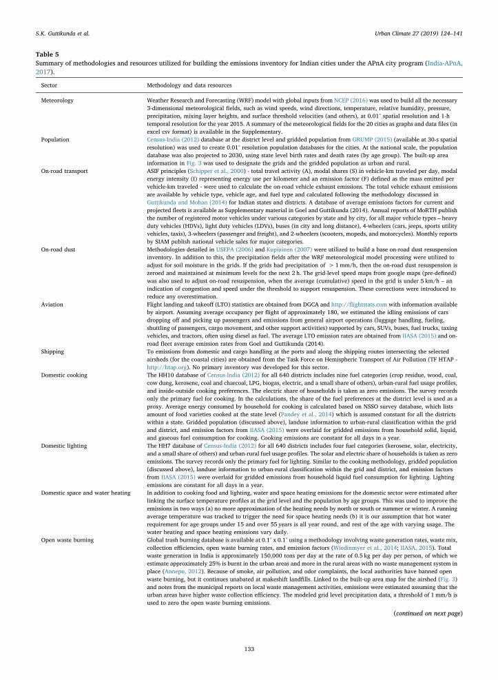
Table 5Summary of methodologies and resources utilized for building the emissions inventory for Indian cities under the APnA city program (India-APnA,2017).

Sector Methodology and data resources

Meteorology Weather Research and Forecasting (WRF) model with global inputs from NCEP (2016) was used to build all the necessary3-dimensional meteorological fields, such as wind speeds, wind directions, temperature, relative humidity, pressure,precipitation, mixing layer heights, and surface threshold velocities (and others), at 0.01° spatial resolution and 1-htemporal resolution for the year 2015. A summary of the meteorological fields for the 20 cities as graphs and data files (inexcel csv format) is available in the Supplementary.

Population Census-India (2012) database at the district level and gridded population from GRUMP (2015) (available at 30-s spatialresolution) was used to create 0.01° resolution population databases for the cities. At the national scale, the populationdatabase was also projected to 2030, using state level birth rates and death rates (by age group). The built-up areainformation in Fig. 3 was used to designate the grids and the gridded population as urban and rural.

On-road transport ASIF principles (Schipper et al., 2000) - total travel activity (A), modal shares (S) in vehicle-km traveled per day, modalenergy intensity (I) representing energy use per kilometer and an emission factor (F) defined as the mass emitted pervehicle-km traveled - were used to calculate the on-road vehicle exhaust emissions. The total vehicle exhaust emissionsare available by vehicle type, vehicle age, and fuel type and calculated following the methodology discussed inGuttikunda and Mohan (2014) for Indian states and districts. A database of average emissions factors for current andprojected fleets is available as Supplementary material in Goel and Guttikunda (2014). Annual reports of MoRTH publishthe number of registered motor vehicles under various categories by state and by city, for all major vehicle types – heavyduty vehicles (HDVs), light duty vehicles (LDVs), buses (in city and long distance), 4-wheelers (cars, jeeps, sports utilityvehicles, taxis), 3-wheelers (passenger and freight), and 2-wheelers (scooters, mopeds, and motorcycles). Monthly reportsby SIAM publish national vehicle sales for major categories.

On-road dust Methodologies detailed in USEPA (2006) and Kupiainen (2007) were utilized to build a base on-road dust resuspensioninventory. In addition to this, the precipitation fields after the WRF meteorological model processing were utilized toadjust for soil moisture in the grids. If the grids had precipitation of > 1mm/h, then the on-road dust resuspension iszeroed and maintained at minimum levels for the next 2 h. The grid-level speed maps from google maps (pre-defined)was also used to adjust on-road resuspension, when the average (cumulative) speed in the grid is under 5 km/h – anindication of congestion and speed under the threshold to support resuspension. These corrections were introduced toreduce any overestimation.

Aviation Flight landing and takeoff (LTO) statistics are obtained from DGCA and http://flightstats.com with information availableby airport. Assuming average occupancy per flight of approximately 180, we estimated the idling emissions of carsdropping off and picking up passengers and emissions from general airport operations (luggage handling, fueling,shuttling of passengers, cargo movement, and other support activities) supported by cars, SUVs, buses, fuel trucks, taxingvehicles, and tractors, often using diesel as fuel. The average LTO emission rates are obtained from IIASA (2015) and on-road fleet average emission rates from Goel and Guttikunda (2014).

Shipping To emissions from domestic and cargo handling at the ports and along the shipping routes intersecting the selectedairsheds (for the coastal cities) are obtained from the Task Force on Hemispheric Transport of Air Pollution (TF HTAP -http://htap.org). No primary inventory was developed for this sector.

Domestic cooking The HH10 database of Census-India (2012) for all 640 districts includes nine fuel categories (crop residue, wood, coal,cow dung, kerosene, coal and charcoal, LPG, biogas, electric, and a small share of others), urban-rural fuel usage profiles,and inside-outside cooking preferences. The electric share of households is taken as zero emissions. The survey recordsonly the primary fuel for cooking. In the calculations, the share of the fuel preferences at the district level is used as aproxy. Average energy consumed by household for cooking is calculated based on NSSO survey database, which listsamount of food varieties cooked at the state level (Pandey et al., 2014) which is assumed constant for all the districtswithin a state. Gridded population (discussed above), landuse information to urban-rural classification within the gridand district, and emission factors from IIASA (2015) were overlaid for gridded emissions from household solid, liquid,and gaseous fuel consumption for cooking. Cooking emissions are constant for all days in a year.

Domestic lighting The HH7 database of Census-India (2012) for all 640 districts includes four fuel categories (kerosene, solar, electricity,and a small share of others) and urban-rural fuel usage profiles. The solar and electric share of households is taken as zeroemissions. The survey records only the primary fuel for lighting. Similar to the cooking methodology, gridded population(discussed above), landuse information to urban-rural classification within the grid and district, and emission factorsfrom IIASA (2015) were overlaid for gridded emissions from household liquid fuel consumption for lighting. Lightingemissions are constant for all days in a year.

Domestic space and water heating In addition to cooking food and lighting, water and space heating emissions for the domestic sector were estimated afterlinking the surface temperature profiles at the grid level and the population by age groups. This was used to improve theemissions in two ways (a) no more approximation of the heating needs by north or south or summer or winter. A runningaverage temperature was tracked to trigger the need for space heating needs (b) it is our assumption that hot waterrequirement for age groups under 15 and over 55 years is all year round, and rest of the age with varying usage. Thewater heating and space heating emissions vary daily.

Open waste burning Global trash burning database is available at 0.1° x 0.1° using a methodology involving waste generation rates, waste mix,collection efficiencies, open waste burning rates, and emission factors (Wiedinmyer et al., 2014; IIASA, 2015). Totalwaste generation in India is approximately 150,000 tons per day at the rate of 0.5 kg per day per person, of which weestimate approximately 25% is burnt in the urban areas and more in the rural areas with no waste management system inplace (Annepu, 2012). Because of smoke, air pollution, and odor complaints, the local authorities have banned openwaste burning, but it continues unabated at makeshift landfills. Linked to the built-up area map for the airshed (Fig. 3)and notes from the municipal reports on local waste management activities, emissions were estimated assuming that theurban areas have higher waste collection efficiency. The modeled grid level precipitation data, a threshold of 1 mm/h isused to zero the open waste burning emissions.

(continued on next page)

S.K. Guttikunda et al. Urban Climate 27 (2019) 124–141

133

5. Modeled particulate sector contributions

5.1. Chemical transport model

We used the Comprehensive Air Quality Model with Extensions (CAMx), to estimate particulate concentrations for each urbanairshed. CAMx is an open-source Eulerian photochemical dispersion model that supports (a) 3-dimensional advection linked to 3-dimensional meteorological data at the grid level, including plume rise calculations for point sources (b) scavenging schematics in theform of dry and wet deposition (c) multiple chemical mechanisms to characterize photochemistry (d) gas to aerosol conversions (fromSO2 to sulfates, NOx to nitrates, and VOCs to secondary organic aerosols) (e) links to online emission calculations for certain sourceslike seasalt and (f) modular processing of area and point sources to estimate contributions by pre-defined region and source. We usethe WRF meteorological model to derive meteorological data (3D wind, temperature, pressure, relative humidity, and precipitationfields) (data files are presented in the Supplementary). The vertical resolution of the model was stretched over 28 layers under 12 km,to improve our simulations of ground level concentrations. The lowest layer is designated at 30m and there are 12 layers within 1 km.

To account for activities outside the designated urban airshed, we use boundary conditions from a model run covering the IndianSubcontinent (details on national emissions inventory and modeling framework are available online @ http://www.indiaairquality.info). We used the MOZART global model to get boundary conditions for the Indian Subcontinent. CAMx modeling system (http://

Table 5 (continued)

Sector Methodology and data resources

Power plants The database of power plants includes geographical location, number of boiler units, coal characteristics, coalconsumption rates, and installed control equipment. These details were documented from their respective environmentalimpact assessment reports and data published by the state electricity boards (public entities) and private operators(Guttikunda and Jawahar, 2014; NPP, 2018). Under NAMP, all the large point sources such as the coal-fired thermalpower plants, are required to conduct continuous emissions monitoring from all the operational stacks, for all the criteriapollutants. However, these emission rates are not public and only reports based on intermittent audits are presented asaverages (MoEFCC, 2010; CEA, 2013; MoEFCC, 2015; CEA, 2017; MoEFCC, 2018). A summary of the emission factorsand an analysis of current and planned power plants is presented in Lu et al. (2013), Guttikunda and Jawahar (2014),Sadavarte and Venkataraman (2014), and IIASA (2015).

Diesel generator sets The spatial allocation of the in-situ emissions from burning of diesel in small and large generator sets was refined usingthe hotspot information available as geospatial layers, including the locations of hotels, hospitals, malls, markets, funeralhomes, religious worship centers, industrial areas, apartment complexes, commercial centers, and telecom towers. Theselayers were extracted from open sources such as Open Street Maps and paid sources such as google API. The shortages inthe power supply at the state and the grid level were sourced from CEA reports, NPP statistics, and load dispatch centerreports. Emission factors by generator set size are summarized in Sahu et al. (2015).

Heavy industries Other than the thermal power plants, details of heavy industries covering fertilizers, cement, refineries, iron and steel,and mineral ore processing were collated using information from respective sector annual reports, http://www.indiastats.com, and emission factors from Sadavarte and Venkataraman (2014) and IIASA (2015). The plant detailsinclude location information and production rates.

Light industries The heavy industries is further substantiated with the industrial fuel consumption data (as solid, liquid, and gaseousfuels) from the Ministry of Statistics, conducted as part of the annual survey of industries (ASI, 2015; MSME, 2017).Broad categories covered under this survey are food processing, textile works, leather works, wood processing, paper andink, coke products, pharmaceuticals, rubber and plastics works, glass works, manufacturing & repairs, power generation,and waste & water treatment. The fuel consumption data by various industrial categories is based on the fuel purchasereceipts at the district level and the emission factors database is from Sadavarte and Venkataraman (2014) and IIASA(2015).

Construction Besides the traditional manufacturing industries, construction is among the fastest growing sectors in India. The demandfor traditional red and fired clay bricks is high, along with cement, and the location of these clusters in and around theurban airsheds were tagged using the open google earth imagery. Most of them are located along the river, with easyaccess to top soil and water for raw material. Traditionally, the rectangle shaped clay bricks are sun dried and readied forfiring in “clamps” - a pile of bricks with intermittent layers of sealing mud and fuel. Technology for firing has changed formass production with the fixed chimney brick kilns having a capacity to produce 10,000 to 20,000 bricks per day (World-Bank, 2010; Mathiel et al., 2012; Guttikunda et al., 2013; Rajarathnam et al., 2014). This fuel would vary fromagricultural waste to biofuels like cow dung and wood to fossil fuels like coal and heavy fuel oil. Emission factors forvarious technologies were summarized from Weyant et al. (2014), IIASA (2015), Akinshipe and Kornelius (2018). Theinventory also includes fugitive dust estimates for construction sites based on empirical functions proposed in USEPA(2006) and operational guidelines from CPCB (2017).

Open fires The location of open fires (from VIIRS and MODIS satellite feeds @ https://worldview.earthdata.nasa.gov), along withpixelated information of landuse fractions (agricultural, forest, urban, water, and arid) were used to estimate the totalemissions. The Fire INventory from NCAR (FINN) model estimates total emissions using these satellite feeds, provideemissions information suitable for chemical transport modeling at a horizontal resolution of 1 sq.km. The global archivesdating back to 2002, along with a database of landuse based emission factors, and data processing procedures to preparemodel ready emission inventory are available @ http://bai.acom.ucar.edu/Data/fire (Akagi et al., 2011; Wiedinmyeret al., 2011).

Dust storms The GOCART dust module from WRF simulates the dust outbreaks and also propagates these emissions in the CAMxdispersion model as a separate source.

Seasalt A CAMx pre-processor calculates seasalt emissions, where applicable, using the 3-dimensional meteorological input forWRF.

S.K. Guttikunda et al. Urban Climate 27 (2019) 124–141

134

www.camx.com) has a pre-processor module to link MOZART model results. The WRF-CAMx modeling system, boundary conditions,and the national emissions inventory for ozone precursor pollutants was evaluated against ground based and satellite observations inSarkar et al., 2016.

The total PM concentrations includes primary aerosols (metals, BC, and OC) and secondary contributions (from chemical con-version of gaseous SO2 to sulfate aerosols and gaseous NOx to nitrate aerosols). In CAMx, the primary PM is modeled in two bins toaccount for differential deposition and advection characteristics – coarse fraction (CPRM) comprises of PM10 to PM2.5 mass and finefraction (FPRM) comprises of everything less than PM2.5 mass. All the secondary aerosols are considered as part of PM2.5 mass. We setup the dispersion model calculations to also estimate sector contributions to ambient PM2.5 concentrations in the urban airshed ofeach city.

Table 6Key household, geography, and transport statistics for 20 Indian cities.

City name A B C D E F G H I J K L

1 Agra 36.2 6.7 37.4 79.7 91.1 33.2 high – 800 – – 0.902 Amritsar 46.9 11.7 58.3 96.0 85.8 26.8 high 120 300 – – 0.933 Bengaluru 44.3 17.5 75.5 98.0 93.3 40.2 low 700 6000 – – 5.564 Bhopal 43.7 12.4 57.8 92.9 74.2 36.2 medium – 400 – – 1.105 Bhubaneswar 33.8 6.8 32.8 71.5 63.8 37.0 medium 160 300 yes – 1.306 Chandigarh 46.7 25.7 71.6 98.4 94.2 40.7 high 160 600 yes – 0.807 Chennai 46.6 13.2 82.4 99.1 94.1 41.0 very low 430 2400 yes yes 4.938 Coimbatore 47.1 9.2 71.5 94.8 81.8 36.2 low 120 6000 yes – 1.909 Dehradun 47.1 14.9 72.4 96.3 90.4 26.5 high 10 750 – – 0.5010 Indore 46.6 10.5 67.8 96.5 78.2 30.2 medium 110 900 yes – 1.7111 Jaipur 45.7 12.5 49.8 86.4 90.2 26.6 high 200 1600 yes – 2.2512 Kanpur 30.3 6.2 51.5 63.0 69.7 35.2 high 125 1200 yes – 1.4613 Kochi 40.7 17.1 63.2 97.4 93.7 6.1 very low 260 400 yes yes 0.6014 Ludhiana 50.4 16.8 68.3 98.3 93.4 29.4 high 190 3000 yes – 1.7715 Nagpur 42.8 7.2 60.2 92.1 69.4 30.0 medium 130 900 yes – 1.3016 Patna 18.4 5.2 33.8 57.1 70.0 30.1 high 310 450 – – 1.0017 Pune 48.8 13.2 67.9 92.7 87.8 46.5 medium 150 3000 yes – 2.3418 Raipur 20.6 3.6 19.4 84.6 47.5 38.7 medium 120 800 yes – 1.8019 Ranchi 25.3 6.1 29.6 63.0 47.7 19.2 high 110 100 – – 0.6020 Varanasi 29.1 4.5 37.4 62.0 77.0 28.5 high 450 200 – – 0.77

Note: A to F statistics are extracted from Census-India (2012). A=% households with at least one motorcycle; B=% households with at least on 4-wheeler (cars and vans); C=% households with primary cooking supported by gas and electricity; D=% households with primary lightingsupported by electricity; E=% households with permanent houses; F=% households with< 2 rooms; G=need for winter heating; H=numberof mapped brick kilns in the city's selected airshed from open google earth imagery; I= number of small scale industries listed under ASI (2015);J= existence of heavy industries (including power plants) in the city's selected airshed; K= coastal or not; L= total number of registered vehiclesin 2015 in millions (MoRTH, 2016).

Table 7Estimated annual emissions totals for the 20 Indian cities in 2015.

Annual emissions (CO2 in million tons/year and rest in tons/year)

City name PM2.5 PM10 BC OC NOx CO NMVOC SO2 CO2

1 Agra 8350 15,600 2100 2950 10,250 79,250 16,400 950 1.552 Amritsar 8600 13,450 2000 2600 12,050 72,100 16,500 2400 2.43 Bengaluru 31,300 67,100 9350 8450 56,900 335,550 83,500 5300 10.424 Bhopal 5900 13,650 1300 1550 8950 54,300 15,100 900 1.655 Bhubaneswar 11,250 22,400 2700 3600 22,250 129,050 27,350 1350 2.286 Chandigarh 18,300 33,600 3450 4850 56,300 160,350 35,850 3200 3.917 Chennai 94,050 132,350 14,500 11,250 207,400 345,550 92,900 26,600 9.768 Coimbatore 14,100 23,900 3500 3050 25,150 113,100 28,200 2650 3.139 Dehradun 4650 7500 1300 1700 7200 39,450 8600 750 1.0410 Indore 11,850 27,600 3250 3150 15,200 83,700 22,250 1400 2.7211 Jaipur 17,200 34,800 4700 5250 20,400 137,600 31,550 2650 3.7912 Kanpur 34,550 43,900 5150 5550 24,750 166,000 34,100 2450 2.3913 Kochi 9150 16,400 2250 2100 63,900 69,550 14,850 20,900 2.414 Ludhiana 14,500 24,200 4550 3850 31,200 128,550 25,900 3750 3.5315 Nagpur 67,100 86,300 6900 7900 128,100 176,850 52,900 9600 6.8916 Patna 18,050 29,500 4800 6150 18,350 171,450 27,650 3850 2.8617 Pune 17,700 36,900 5600 4150 37,000 166,050 41,900 3950 5.8118 Raipur 41,500 59,650 9150 9050 60,700 163,300 118,150 7600 3.1319 Ranchi 13,150 24,300 3350 4550 13,150 128,500 25,300 1950 2.3120 Varanasi 12,100 17,450 3050 4850 14,050 134,400 21,850 2300 1.79

S.K. Guttikunda et al. Urban Climate 27 (2019) 124–141

135

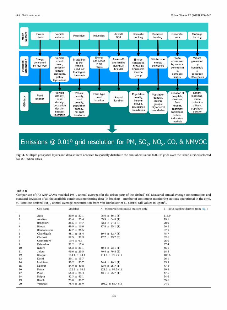
Fig. 4. Multiple geospatial layers and data sources accessed to spatially distribute the annual emissions to 0.01° grids over the urban airshed selectedfor 20 Indian cities.

Table 8Comparison of (A) WRF-CAMx modeled PM2.5 annual average (for the urban parts of the airshed) (B) Measured annual average concentrations andstandard deviation of all the available continuous monitoring data (in brackets – number of continuous monitoring stations operational in the city).(C) satellite-derived PM2.5 annual average concentration from van Donkelaar et al. (2016) (all values in μg/m3).

City name Modeled A - Measured (continuous stations only) B – 2016 satellite-derived from Fig. 1

1 Agra 89.0 ± 27.1 98.6 ± 86.1 (1) 116.92 Amritsar 83.4 ± 25.4 65.9 ± 64.8 (1) 79.13 Bengaluru 36.5 ± 19.7 32.3 ± 24.2 (3) 28.94 Bhopal 49.9 ± 16.0 47.8 ± 35.1 (1) 56.55 Bhubaneswar 47.7 ± 26.5 37.96 Chandigarh 58.1 ± 18.4 59.4 ± 62.7 (1) 78.77 Chennai 57.5 ± 31.3 47.7 ± 73.7 (3) 32.68 Coimbatore 19.4 ± 9.5 26.09 Dehradun 51.2 ± 17.6 87.410 Indore 66.3 ± 31.1 40.4 ± 23.1 (1) 46.111 Jaipur 99.6 ± 29.5 70.4 ± 76.8 (3) 68.312 Kanpur 114.1 ± 44.4 111.4 ± 79.7 (1) 106.613 Kochi 29.1 ± 15.7 26.114 Ludhiana 90.2 ± 33.7 74.4 ± 46.1 (1) 83.915 Nagpur 84.9 ± 40.8 53.9 ± 26.7 (1) 47.316 Patna 122.2 ± 68.2 121.3 ± 89.5 (1) 90.817 Pune 56.3 ± 28.4 43.1 ± 25.7 (1) 47.518 Raipur 82.3 ± 43.1 54.619 Ranchi 73.0 ± 36.7 55.620 Varanasi 78.4 ± 26.9 106.2 ± 83.4 (1) 94.0

S.K. Guttikunda et al. Urban Climate 27 (2019) 124–141

136

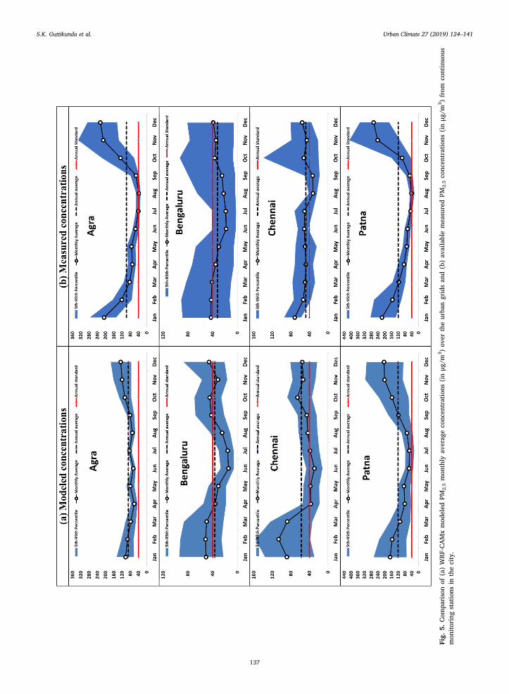
Fig.

5.Com

parisonof

(a)WRF-CAMxmod

eled

PM2.5

mon

thly

averag

eco

ncen

trations

(inμg

/m3)ov

ertheurba

ngridsan

d(b)av

ailablemeasuredPM

2.5

conc

entrations

(inμg

/m3)from

continuo

usmon

itoringstations

inthecity.

S.K. Guttikunda et al. Urban Climate 27 (2019) 124–141

137

5.2. Modeled particulate concentrations

Table 8 summarizes the modeled annual average PM2.5 concentrations. We also present PM concentration maps in Fig. 3(d) forAgra, Bengaluru, Chennai, and Patna. Concentration maps for all the 20 cities are presented in the Supplementary. Except forCoimbatore and Bengaluru (both from Southern India), all the urban airsheds exceed the national annual standard of 40 μg/m3 forPM2.5.

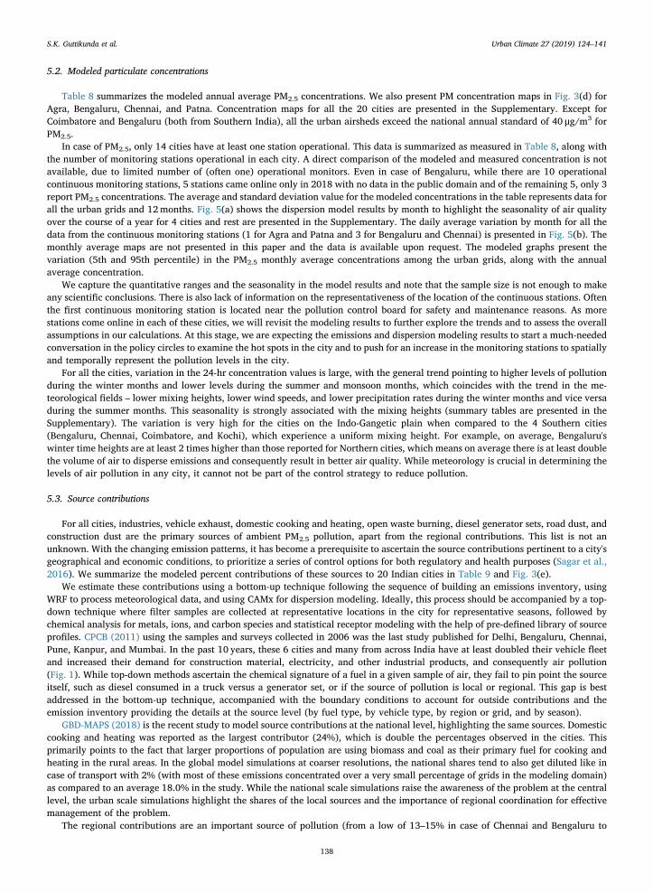
In case of PM2.5, only 14 cities have at least one station operational. This data is summarized as measured in Table 8, along withthe number of monitoring stations operational in each city. A direct comparison of the modeled and measured concentration is notavailable, due to limited number of (often one) operational monitors. Even in case of Bengaluru, while there are 10 operationalcontinuous monitoring stations, 5 stations came online only in 2018 with no data in the public domain and of the remaining 5, only 3report PM2.5 concentrations. The average and standard deviation value for the modeled concentrations in the table represents data forall the urban grids and 12months. Fig. 5(a) shows the dispersion model results by month to highlight the seasonality of air qualityover the course of a year for 4 cities and rest are presented in the Supplementary. The daily average variation by month for all thedata from the continuous monitoring stations (1 for Agra and Patna and 3 for Bengaluru and Chennai) is presented in Fig. 5(b). Themonthly average maps are not presented in this paper and the data is available upon request. The modeled graphs present thevariation (5th and 95th percentile) in the PM2.5 monthly average concentrations among the urban grids, along with the annualaverage concentration.

We capture the quantitative ranges and the seasonality in the model results and note that the sample size is not enough to makeany scientific conclusions. There is also lack of information on the representativeness of the location of the continuous stations. Oftenthe first continuous monitoring station is located near the pollution control board for safety and maintenance reasons. As morestations come online in each of these cities, we will revisit the modeling results to further explore the trends and to assess the overallassumptions in our calculations. At this stage, we are expecting the emissions and dispersion modeling results to start a much-neededconversation in the policy circles to examine the hot spots in the city and to push for an increase in the monitoring stations to spatiallyand temporally represent the pollution levels in the city.

For all the cities, variation in the 24-hr concentration values is large, with the general trend pointing to higher levels of pollutionduring the winter months and lower levels during the summer and monsoon months, which coincides with the trend in the me-teorological fields – lower mixing heights, lower wind speeds, and lower precipitation rates during the winter months and vice versaduring the summer months. This seasonality is strongly associated with the mixing heights (summary tables are presented in theSupplementary). The variation is very high for the cities on the Indo-Gangetic plain when compared to the 4 Southern cities(Bengaluru, Chennai, Coimbatore, and Kochi), which experience a uniform mixing height. For example, on average, Bengaluru'swinter time heights are at least 2 times higher than those reported for Northern cities, which means on average there is at least doublethe volume of air to disperse emissions and consequently result in better air quality. While meteorology is crucial in determining thelevels of air pollution in any city, it cannot not be part of the control strategy to reduce pollution.

5.3. Source contributions

For all cities, industries, vehicle exhaust, domestic cooking and heating, open waste burning, diesel generator sets, road dust, andconstruction dust are the primary sources of ambient PM2.5 pollution, apart from the regional contributions. This list is not anunknown. With the changing emission patterns, it has become a prerequisite to ascertain the source contributions pertinent to a city'sgeographical and economic conditions, to prioritize a series of control options for both regulatory and health purposes (Sagar et al.,2016). We summarize the modeled percent contributions of these sources to 20 Indian cities in Table 9 and Fig. 3(e).

We estimate these contributions using a bottom-up technique following the sequence of building an emissions inventory, usingWRF to process meteorological data, and using CAMx for dispersion modeling. Ideally, this process should be accompanied by a top-down technique where filter samples are collected at representative locations in the city for representative seasons, followed bychemical analysis for metals, ions, and carbon species and statistical receptor modeling with the help of pre-defined library of sourceprofiles. CPCB (2011) using the samples and surveys collected in 2006 was the last study published for Delhi, Bengaluru, Chennai,Pune, Kanpur, and Mumbai. In the past 10 years, these 6 cities and many from across India have at least doubled their vehicle fleetand increased their demand for construction material, electricity, and other industrial products, and consequently air pollution(Fig. 1). While top-down methods ascertain the chemical signature of a fuel in a given sample of air, they fail to pin point the sourceitself, such as diesel consumed in a truck versus a generator set, or if the source of pollution is local or regional. This gap is bestaddressed in the bottom-up technique, accompanied with the boundary conditions to account for outside contributions and theemission inventory providing the details at the source level (by fuel type, by vehicle type, by region or grid, and by season).

GBD-MAPS (2018) is the recent study to model source contributions at the national level, highlighting the same sources. Domesticcooking and heating was reported as the largest contributor (24%), which is double the percentages observed in the cities. Thisprimarily points to the fact that larger proportions of population are using biomass and coal as their primary fuel for cooking andheating in the rural areas. In the global model simulations at coarser resolutions, the national shares tend to also get diluted like incase of transport with 2% (with most of these emissions concentrated over a very small percentage of grids in the modeling domain)as compared to an average 18.0% in the study. While the national scale simulations raise the awareness of the problem at the centrallevel, the urban scale simulations highlight the shares of the local sources and the importance of regional coordination for effectivemanagement of the problem.

The regional contributions are an important source of pollution (from a low of 13–15% in case of Chennai and Bengaluru to

S.K. Guttikunda et al. Urban Climate 27 (2019) 124–141

138

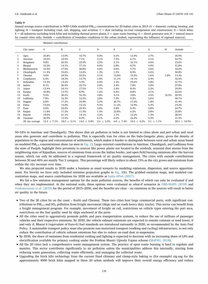
50–52% in Amritsar and Chandigarh). This shows that air pollution in India is not limited to cities alone and peri urban and ruralareas also generate and contribute to pollution. This is especially true for cities on the Indo-Gangetic plain, given the density ofpopulation in the region and concentration of settlements, which makes it harder to distinguish between rural and urban areas basedon modeled PM2.5 concentrations alone (as seen in Fig. 1). Large external contributions in Amritsar, Chandigarh, and Ludhiana fromthe state of Punjab, highlight their proximity to sources like power plants not located in the airsheds, seasonal dust storms from theneighboring state of Rajasthan, sources of emissions from across the Indian border, and open field burning emissions after the harvestseason, which can only be addressed in a regional framework of air quality management. The cities with outside contributionsbetween 30 and 40% are mostly Tier 2 category. This percentage will likely reduce to about 15% as the city grows and emissions fromwithin the city increase over time.

We also projected results to 2030 under a business as usual scenario by modeling emissions, dispersion, and source apportion-ment. For brevity we have only included emission projection graphs in Fig. 3(b). The gridded emission maps, and modeled con-centration maps, and source contributions for 2030 are available at India-APnA (2017).

We list a few emission management options for the main pollution sources, the benefits of which can only be evaluated if andwhen they are implemented. At the national scale, these options were evaluated as what-if scenarios in GBD-MAPS (2018) andVenkataraman et al. (2018) for the period of 2015–2050, and the benefits are clear – no emissions at the sources will result in betterair quality in the future.

• Two of the 20 cities lie on the coast – Kochi and Chennai. These two cities host large commercial ports, with significant con-tributions to PM2.5 and SO2 pollution from freight movement (ships and on roads heavy duty trucks). This sector can benefit froma freight management program. For example, movement of freight on rail, restrictions on vehicle types entering the port area,restrictions on the fuel quality used by ships anchored at the ports.

• All the cities need to aggressively promote public and para transportation systems, to reduce the use of millions of passengervehicles and their respective emissions. By 2030, the vehicle exhaust emissions are expected to remain constant or tend lower, ifand only if, Bharat 6 (equivalent of Euro-6) fuel standards are introduced nationally in 2020, as recommended by the Auto FuelPolicy. A sustainable transport policy must also promote non-motorized transport (walking and cycling) infrastructure, to not onlyreduce the contribution of vehicle exhaust emissions but also to reduce on-road dust re-suspension.

• By 2030, the share of emissions from residential cooking and lighting is expected to decrease with an increasing share of LPG andelectrification available for primary cooking under the Prathan Mantri Ujjwala Yojana scheme (MoPNG, 2018).

• All the 20 cities lack a comprehensive waste management system. The practice of open waste burning is hard to regulate andmonitor. This sector contributes significantly to air pollution unless the municipalities address this internally, starting fromreducing waste generation, collecting waste efficiently, and managing the collected waste.

• Upgrading the brick kiln technology from the current fixed chimney and clamp-style baking to (for example) zig-zag for theapproximately 4000 brick kilns mapped in these 20 urban airsheds will improve their overall energy efficiency and reduce

Table 9Annual average source contributions to WRF-CAMx modeled PM2.5 concentrations for 20 Indian cities in 2015 (A=domestic cooking, heating, andlighting; B= transport including road, rail, shipping, and aviation; C= dust including on-road resuspension and construction; D=brick kilns;E= all industries excluding brick kilns and including thermal power plants; F= open waste burning; G=diesel generator sets; H= natural sourcefor coastal cities only; Outside= contribution of boundary conditions to the urban airshed, representing the influence of regional sources).

Modeled contributions

City name A B C D E F G H Outside

1 Agra 23.8% 13.9% 10.7% 0.0% 0.2% 12.4% 2.7% 35.9%2 Amritsar 10.6% 10.5% 7.1% 2.1% 7.3% 6.1% 3.1% 52.7%3 Bengaluru 9.8% 26.5% 23.0% 2.5% 2.1% 16.1% 4.0% 15.6%4 Bhopal 10.2% 14.1% 17.1% 0.0% 2.8% 8.7% 4.9% 41.8%5 Bhubaneswar 15.9% 17.0% 20.8% 4.0% 0.6% 5.7% 3.6% 32.0%6 Chandigarh 11.4% 10.6% 12.6% 1.3% 1.3% 8.9% 2.6% 50.8%7 Chennai 3.6% 24.5% 23.5% 3.1% 12.8% 15.5% 1.6% 1.8% 13.3%8 Coimbatore 6.4% 18.3% 13.7% 1.0% 11.1% 14.1% 2.4% 32.5%9 Dehradun 14.3% 14.2% 4.4% 0.4% 1.3% 19.6% 3.8% 41.7%10 Indore 8.1% 26.9% 22.7% 2.0% 2.4% 7.8% 2.0% 27.8%11 Jaipur 13.4% 24.1% 17.5% 1.7% 2.4% 8.4% 2.2% 29.9%12 Kanpur 33.8% 13.7% 8.9% 1.2% 6.5% 8.8% 4.1% 22.5%13 Kochi 9.5% 20.2% 16.3% 3.8% 4.1% 3.8% 4.5% 16.5% 20.9%14 Ludhiana 7.8% 16.3% 12.3% 2.8% 7.9% 9.2% 2.6% 40.7%15 Nagpur 6.8% 17.2% 10.9% 3.2% 26.7% 11.6% 1.8% 21.4%16 Patna 14.6% 14.8% 12.1% 9.3% 11.2% 12.9% 5.4% 19.2%17 Pune 5.8% 24.0% 23.4% 2.6% 9.8% 6.4% 2.8% 24.7%18 Raipur 11.8% 17.2% 11.5% 1.4% 22.8% 6.2% 2.8% 25.8%19 Ranchi 18.0% 21.1% 14.1% 3.2% 1.1% 12.2% 1.3% 28.5%20 Varanasi 20.9% 13.5% 8.2% 6.1% 0.2% 16.2% 3.3% 31.2%

20 city average 12.9 ± 7.1% 18.0 ± 5.1% 14.6 ± 5.8% 2.6 ± 2.2% 6.8 ± 7.4% 10.6 ± 4.2% 3.1 ± 1.1% 30.5 ± 10.9%

S.K. Guttikunda et al. Urban Climate 27 (2019) 124–141

139

emission loads (World-Bank, 2010; Maithel et al., 2012).

• Coal-fired power plants and large industries with captive power plants need to enforce stricter emission standards for all thecriteria pollutants to reduce their share of influence on urban air quality. The densely populated Indo-Gangetic plain has cities andrural areas near these large point sources that strongly influences each other's ambient air quality (Guttikunda and Jawahar,2014).

• A regional air quality management, spanning multiple states, districts, and stakeholders is necessary to reduce the pollution loadsfor all the cities. In April 2018, draft of the National Clean Air Programme (NCAP) is a step in the right direction designed to buildinstitutional and technical capacity of CPCB and SPCBs “to meet the prescribed annual average ambient air quality standards at alllocations in the country in a stipulated timeframe” (CPCB, 2018).

6. Policy implications of a knowledge base

In policy circles, the debate on air quality in India and how to best tackle it, is limited to metropolitan cities. Yet, India lives in itsvillages and smaller towns. We need to look at the state of air pollution in Tier 1 and 2 cities, quantify its extent and understand itssources. With a growth in population and ever-increasing concentration of settlements (especially in the Indo-Gangetic plain), theneed for baselines and a start to tackle air pollution is urgent. In the short term, there is an immediate need to increase the groundlevel monitoring network, which can further support establishing air pollution trend lines for the cities and help monitor action plans.

Urban India is growing rapidly and infrastructure and management systems are yet to catchup with growing urban population,more waste generation (per capita and totals), greater share of motorized transport for individual and commercial purposes, anincrease in industrial and manufacturing activity, and a growing demand for clean fuels for cooking and heating. With the lack ofsystems, cities resort to ad-hoc methods to deal with increased pressure on existing infrastructure. Hence cities need to start planningby anticipating the challenges they will face as they grow and be proactive about solutions to reduce air pollution.

For most of the cities in this study, this is the first time an emissions inventory has been built for the city, followed by a dispersionmodeling exercise to assess the particulate pollution trend and identify source contributions. Local governments can use thesenumbers as a start to develop an air pollution control policy. Apart from numbers, identifying the spatial spread in pollution hotspotslends itself to immediate action. With information, cities can plan for the long-term action by simulating different scenarios that arecustomized to each city. Simply publishing these numbers will not reduce pollution. But in the absence of any other concreteinformation, results from this study can support the policy makers establish baselines and plot a roadmap to improve air quality in thelong run.

While the analysis presented in this paper focused on the long-term air pollution knowledge assessment, we use the same in-formation base for on-going short-term air quality forecasting (for 3-days) releasing data on an open platform (details @ http://www.indiaairquality.info).

Acknowledgements

We would like to thank the Shakti Sustainable Energy Foundation (SSEF, New Delhi, India) for supporting the India-APnA cityprogram.

Appendix A. Supplementary data

Supplementary data associated with this article can be found in the online version, at doi: https://doi.org/10.1016/j.uclim.2018.11.005. These data include the Google maps of the most important areas described in this article.

References

Akagi, S.K., Yokelson, R.J., Wiedinmyer, C., Alvarado, M.J., Reid, J.S., Karl, T., Crounse, J.D., Wennberg, P.O., 2011. Emission factors for open and domestic biomassburning for use in atmospheric models. Atmos. Chem. Phys. 11, 4039–4072.

Akinshipe, O., Kornelius, G., 2018. Quantification of atmospheric emissions and energy metrics from simulated clamp kiln technology in the clay brick industry.Environ. Pollut. 236, 580–590.

Annepu, R.K., 2012. Sustainable Solid Waste Management in India. Masters Thesis. Earth Engineering Center, Columbia University, New York, USA.ASI, 2015. Annual Survey of Industries, New Delhi, India.Brauer, M., Freedman, G., Frostad, J., van Donkelaar, A., Martin, R.V., Dentener, F., Dingenen, R.v., Estep, K., Amini, H., Apte, J.S., Balakrishnan, K., Barregard, L.,

Broday, D., Feigin, V., Ghosh, S., Hopke, P.K., Knibbs, L.D., Kokubo, Y., Liu, Y., Ma, S., Morawska, L., Sangrador, J.L.T., Shaddick, G., Anderson, H.R., Vos, T.,Forouzanfar, M.H., Burnett, R.T., Cohen, A., 2016. Ambient air pollution exposure estimation for the global burden of disease 2013. Environ. Sci. Technol. 50,79–88.

CEA, 2013. All India Electricity Statistics - General Review 2012, New Delhi, India.CEA, 2017. All India Electricity Statistics - General Review 2016, New Delhi, India.Census-India, 2012. Census of India 2011, 15th Edition. The Ministry of Home Affairs, Government of India, New Delhi, India.CPCB, 2003. Guidelines for Ambient Air Quality Monitoring. Ministry of Environment, Forest, and Climate Change (MoEFCC). Government of India, New Delhi, India.CPCB, 2011. Air Quality Monitoring, Emission Inventory and Source Apportionment Study for Indian Cities. Central Pollution Control Board. Government of India,

New Delhi, India.CPCB, 2017. Guidelines on Environmental Management of Construction & Demolition and Wastes. Ministry of Environment, Forest, and Climate Change (MoEFCC).

Government of India, New Delhi, India.CPCB, 2018. National Clean Air Programme (NCAP) - India. Ministry of Environment, Forest, and Climate Change (MoEFCC). Government of India, New Delhi, India.GBD, 2018. The Global Burden of Disease 2010: Generating Evidence and Guiding Policy. Institute for Health Metrics and Evaluation, Seattle, USA.

S.K. Guttikunda et al. Urban Climate 27 (2019) 124–141

140

GBD-MAPS, 2018. Burden of disease attributable to major air pollution sources in India. Health Effects Institute, Boston, USA.Goel, R., Guttikunda, S.K., 2015. Evolution of on-road vehicle exhaust emissions in Delhi. Atmos. Environ. 105, 78–90.GRUMP, 2015. Gridded Population of the World and Global Rural and Urban Mapping Project. Center for International Earth Science Information Network (CIESIN) of

the Earth Institute, Columbia University, New York, U. S. A.Guttikunda, S.K., Calori, G., 2013. A GIS based emissions inventory at 1 km - 1 km spatial resolution for air pollution analysis in Delhi, India. Atmos. Environ. 67,

101–111.Guttikunda, S.K., Jawahar, P., 2012. Application of SIM-air modeling tools to assess air quality in Indian cities. Atmos. Environ. 62, 551–561.Guttikunda, S.K., Jawahar, P., 2014. Atmospheric emissions and pollution from the coal-fired thermal power plants in India. Atmos. Environ. 92, 449–460.Guttikunda, S.K., Kopakka, R.V., 2014. Source emissions and health impacts of urban air pollution in Hyderabad, India. Air Quality Atmos. Health 7, 195–207.Guttikunda, S.K., Mohan, D., 2014. Re-fueling road transport for better air quality in India. Energy Policy 68, 556–561.Guttikunda, S.K., Begum, B.A., Wadud, Z., 2013. Particulate pollution from brick kiln clusters in the Greater Dhaka region, Bangladesh. Air Quality Atmos. Health 6,

357–365.Guttikunda, S.K., Goel, R., Pant, P., 2014. Nature of air pollution, emission sources, and management in the Indian cities. Atmos. Environ. 95, 501–510.IIASA, 2015. Greenhouse Gas and Air Pollution Interactions and Synergies - South Asia Program. International Institute of Applied Systems Analysis, Laxenburg,

Austria.India-APnA, 2017. Air Pollution Knowledge Assessments (APnA) City Program. Urban Emissions Info, New Delhi, India.Kupiainen, K., 2007. Road dust from pavement wear and traction sanding. Monographs of the Boreal Environment Research, No. 26. Finnish Environmental Institute,

Helsinki, Finland.Landscan, 2013. Gridded Global Population Database. Developed by the Department of Energy's Oak Ridge National Laboratory. Distributed by East View Information

Services, U.S.A.Lu, Z., Streets, D.G., de Foy, B., Krotkov, N.A., 2013. Ozone monitoring Instrument observations of interannual increases in SO2 emissions from Indian coal-fired power

plants during 2005-2012. Environ. Sci. Technol. 47, 13993–14000.Maithel, S., Uma, R., Bond, T., Baum, E., Thao, V.T.K., 2012. Brick kilns performance assessment, emissions measurements, & a roadmap for cleaner brick production

in India. In: Study Report Prepared by Green Knowledge Solutions, New Delhi, India.MoEFCC, 2010. Environmental Impact Assessment Guidelines for Thermal Power Plants. Ministry of Environment and Forests, the Government of India, New Delhi,

India.MoEFCC, 2015. Environment Standards for Thermal Power Plants Along With the Corrigendum, S.O.3305(E), Ministry of Environment and Forests, The Government of

India, New Delhi, India.MoEFCC, 2018. Reports at Environmental Impact Assessment Division. Ministry of Environment and Forests, the Government of India, New Delhi, India.MoPNG, 2018. Prathan Mantri Ujjwala Yojana (PMUY). Ministry of Petroleum and National Gas, Government of India, New Delhi, India.MoRTH, 2016. Annual Report 2016. Ministry of Road Transport and Highways, Government of India, New Delhi, India.MSME, 2017. District Industrial Profile. Miro, Small, and Medium Enterprises (MSME) - Development Institute. Ministry of MSME, Government of India, Bengaluru,

India.NCEP, 2016. National Centers for Environmental Prediction. In: National Oceanic and Atmospheric Administration. U. S. A, Maryland.NPP, 2018. National power portal by central electrical authority. Ministry of Power. In: Government of India. India, New Delhi.Pandey, A., Sadavarte, P., Rao, A.B., Venkataraman, C., 2014. Trends in multi-pollutant emissions from a technology-linked inventory for India: II. Residential,

agricultural and informal industry sectors. Atmos. Environ. 99, 341–352.Pant, P., Harrison, R.M., 2012. Critical review of receptor modelling for particulate matter: a case study of India. Atmos. Environ. 49, 1–12.Pesaresi, M., Ehrlich, D., Florczyk, A.J., Freire, S., Julea, A., Kemper, T., Syrris, V., 2016. The global human settlement layer from landsat imagery, Geoscience and

Remote Sensing Symposium (IGARSS). 2016 IEEE International. IEEE 7276–7279.Rajarathnam, U., Athalye, V., Ragavan, S., Maithel, S., Lalchandani, D., Kumar, S., Baum, E., Weyant, C., Bond, T., 2014. Assessment of air pollutant emissions from

brick kilns. Atmos. Environ. 98, 549–553.Sadavarte, P., Venkataraman, C., 2014. Trends in multi-pollutant emissions from a technology-linked inventory for India: I. Industry and transport sectors. Atmos.

Environ. 99, 353–364.Sagar, A., Balakrishnan, K., Guttikunda, S., Roychowdhury, A., Smith, K.R., 2016. India leads the way: a health-centered strategy for air pollution. Environ. Health

Perspect. 124, A116.Sahu, S.K., Schultz, M.G., Beig, G., 2015. Critical pollutant emissions from the Indian telecom network. Atmos. Environ. 103, 34–42.Sarkar, M., Venkataraman, C., Guttikunda, S., Sadavarte, P., 2016. Indian emissions of technology-linked NMVOCs with chemical speciation: an evaluation of the

SAPRC99 mechanism with WRF-CAMx simulations. Atmos. Environ. 134, 70–83.Schipper, L., Marie-Lilliu, C., Gorham, R., 2000. Flexing the Link between Transport and Greenhouse Gas Emissions: A Path for the World Bank. International Energy

Agency, Paris, France.Shaddick, G., Thomas, M., Amini, H., Broday, D.M., Cohen, A., Frostad, J., Green, A., Gumy, S., Liu, Y., Martin, R.V., Simpson, D., van Donkelaar, A., Brauer, M., 2018.

Data integration for the assessment of population exposure to ambient air pollution for global burden of disease assessment. In: Environmental Science &Technology.

USEPA, 2006. Clearinghouse for Inventories & Emissions Factors - AP 42, fifth ed. United States Environmental Protection Agency, Washington DC, USA.Van Donkelaar, A., Martin, R.V., Brauer, M., Hsu, N.C., Kahn, R.A., Levy, R.C., Lyapustin, A., Sayer, A.M., Winker, D.M., 2016. Global estimates of fine particulate

matter using a combined geophysical-statistical method with information from satellites, models, and monitors. Environ. Sci. Technol. 50, 3762–3772.Venkataraman, C., Brauer, M., Tibrewal, K., Sadavarte, P., Ma, Q., Cohen, A., Chaliyakunnel, S., Frostad, J., Klimont, Z., Martin, R.V., 2018. Source influence on

emission pathways and ambient PM2.5 pollution over India (2015–2050). Atmos. Chem. Phys. 18, 8017–8039.Weyant, C., Athalye, V., Ragavan, S., Rajarathnam, U., Lalchandani, D., Maithel, S., Baum, E., Bond, T.C., 2014. Emissions from South Asian Brick Production. Environ.

Sci. Technol. 48, 6477–6483.WHO, 2016. Global Health Observatory data - Mortality and burden of disease from ambient air pollution. http://www.who.int/gho/phe/outdoor_air_pollution/

burden/en/ last accessed July 8th, 2018. World Health Organization, Geneva, Switzerland.WHO, 2018. WHO Global Ambient Air Quality Database (Update 2018). World Health Organization, Geneva, Switzerland.Wiedinmyer, C., Akagi, S.K., Yokelson, R.J., Emmons, L.K., Al-Saadi, J.A., Orlando, J.J., Soja, A.J., 2011. The Fire INventory from NCAR (FINN): a high resolution

global model to estimate the emissions from open burning. Geosci. Model Dev. 4, 625–641.Wiedinmyer, C., Yokelson, R.J., Gullett, B.K., 2014. Global emissions of trace gases, particulate matter, and hazardous air pollutants from open burning of domestic

waste. Environ. Sci. Technol. 48, 9523–9530.World-Bank, 2010. Vertical Shaft Brick Kiln - Design Manual. ESMAP Publication Series. The World Bank, Washington DC, USA.

S.K. Guttikunda et al. Urban Climate 27 (2019) 124–141

141