Air gap spinning of cellulose fibers from ionic solvents

Master of Science Thesis [in the Master Degree Program, Advanced

materials]

Artur Hedlund

Department of Chemistry

Division of Polymer science

CHALMERS UNIVERSITY OF TECHNOLOGY

Gothenburg, Sweden, 2013

Här finns utrymme att lägga in en bild.

Tänk bara på att anpassa så att nedersta

textraden ligger kvar i nederkant.

Abstract

Dissolving-pulp was dissolved up to >15 wt% in EmimAc an ionic liquid very efficient for

dissolving cellulose. Air-gap spinning, the method of choice for very viscous solutions and for

obtaining strong fibers was applied in lab-scale with limited success. It was found that air-gap

spinning requires many parameters to be paid attention to. Many practical problems were

encountered why no stable spinning was achieved. However a glimpse of the potential was

seen (tenacities>25cN/tex under poorly controlled conditions). This work also contains

accounts of much of the pertinent theory and of most of the problems that are run into if

trying to air-gap spin cellulose-ionic liquid solutions. Not least was it demonstrated how

difficult it is to bring industrial methods, such as falling jet-type spin baths, down to lab-scale

where mass-flows and spinning speeds are much lower than in industry.

Contents

INTRODUCTION ................................................................................................................................................ 2

1 THEORY ............................................................................................................................................................ 3 1.1 SOME USEFUL THEORY ON POLYMERS .......................................................................................................................... 3

1.1.1 Some generalities .............................................................................................................................................................. 3 1.1.2 The physical states of polymers .................................................................................................................................. 3 1.1.3 Flow in polymers ............................................................................................................................................................... 4

Elongational flow ................................................................................................................................................................................................................... 5

1.1.4 Solubility and precipitation.......................................................................................................................................... 6 1.1.5 Crystallization and order ............................................................................................................................................. 8 1.1.6 Mesophases and orientation ........................................................................................................................................ 9

1.2 CELLULOSE ....................................................................................................................................................................... 9 1.3 IONIC LIQUIDS .............................................................................................................................................................. 12

1.3.1 Melting temperature .................................................................................................................................................... 13 1.3.2 Thermal stability ............................................................................................................................................................ 14 1.3.3 Viscosity .............................................................................................................................................................................. 14 1.3.4 Polarity ............................................................................................................................................................................... 15 1.3.5 surface tension................................................................................................................................................................. 15 1.3.6 In a cellulose context .................................................................................................................................................... 16

1.3.6.1 Generalities ............................................................................................................................................................................................................ 16 1.3.6.2 Reported trials of spinning cellulose-IL solutions............................................................................................................................... 16

1.4 THREE RELATED FIBERS .............................................................................................................................................. 17 1.4.1 Lessons from Kevlar ...................................................................................................................................................... 18

1.4.1.1 Some justification for the comparison ...................................................................................................................................................... 18 1.4.1.2 Structure and morphology.............................................................................................................................................................................. 19 1.4.1.3 Ruptures ................................................................................................................................................................................................................. 20

1.4.2 Mono/poly-phosphoric acid ..................................................................................................................................... 20 1.4.3 NMMO-Lyocell .................................................................................................................................................................. 21

1.4.3.1 The dope .................................................................................................................................................................................................................. 22 1.4.3.2 Spinning ................................................................................................................................................................................................................... 23 1.4.3.3 Coagulation ........................................................................................................................................................................................................... 24 1.4.3.4 Structure ................................................................................................................................................................................................................. 26 1.4.3.5 Fibrillation ............................................................................................................................................................................................................. 27

1.5 SUMMARY OF BASIC FLOW THEORY ........................................................................................................................... 27 1.5.1 Shear flow in die ............................................................................................................................................................. 27 1.5.2 Elongational flow in airgap ...................................................................................................................................... 29

2 PRACTICAL WORK ..................................................................................................................................... 34 2.1 CONSTRUCTION OF EQUIPMENT ................................................................................................................................. 35 2.2 DISSOLVING ................................................................................................................................................................... 36 2.3 SPINNING ...................................................................................................................................................................... 38 2.4 MEASUREMENTS AND TESTING .................................................................................................................................. 41

3 RESULTS AND DISCUSSION .................................................................................................................... 42 3.1 DSC ................................................................................................................................................................................. 42 3.2 VISCOSIMETRY ............................................................................................................................................................. 44 3.3 DENSITY ......................................................................................................................................................................... 46 3.4 MEASUREMENTS ON FIBERS ....................................................................................................................................... 49

4 CONCLUSION ................................................................................................................................................ 52

5 FURTHER DEVELOPMENT ....................................................................................................................... 53

6 REFERENCES ................................................................................................................................................ 54

Introduction

Of all organic matter on earth, cellulose is the most common. It is estimated that about 150

billion tons is formed and decomposed in natural processes annually. It is the natural and very

efficient reinforcement of all plants, from the logs of trees to the straws of grass. There it is

incorporated in a natural composite with lignin and hemicellulose. In some processes such as

paper production it as been successfully removed from that matrix, or it can be used directly

in the form of wood. [1]

However cellulose is a stiff and strong polymer and in a future of lacking petroleum, it is a

very attractive prospect to use it as such. While most polymers melt somewhere in the range

100-300°C, cellulose unfortunately does not. Therefore any shaping requires its dissolution,

which it is generally very resistant to. Certain ionic liquids, having very particular chemical

characteristics, have come up as an efficient alternative for doing so, looking more promising

than many earlier methods.

A relatively simple but attractive and useful shape to create from polymer solutions is a fiber.

That is the result if the solution is extruded through a narrow opening into some media, which

causes it to precipitate (coagulate/regenerate), a process termed wet-spinning. Instead of

extruding it directly into the bath, it may first be passed through an inert gas before being

immersed and precipitated. Such a volume of air is called an air-gap and in it, the extruded,

flowing mass can be deformed by axial forces parallel to the flow-direction. This is called air-

gap spinning or air-gap wet-spinning.

Particularly it is well known that such flows control the molecular orientation and

consequently most of the central properties like, strength, crystallinity and stiffness of fibers.

This text contains both literary and

practical studies on combining IL-

cellulose solutions with the air-gap wet-

spinning technique. While initially

aiming at producing actual fibers, it has

rather evolved into an introductory study for such work,

due to the width of the task. May it

contain a good collection of useful

information and experience as a

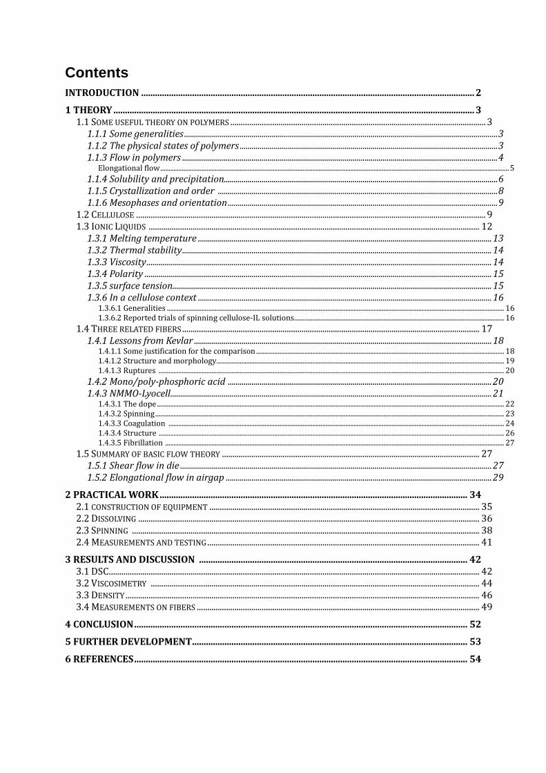
Figure 1: A typical example of how a falling-jet bath is schematically represented in literature.

foundation for further work.

1 Theory

1.1 Some useful theory on polymers

In this section some concepts and theories, which are helpful for the understanding of this

work will be presented in a rather condensed form. For readers already well acquainted with

the subject this section may be skipped. A useful reference when writing this section was “the

physics of polymers” by Strobl [2], so unless otherwise stated it is the origin.

1.1.1 Some generalities

In a polymer melt or solution its molecules are generally considered (the Rouse model) as a

chain of Nb straight but elastic segments composed of several monomers whose orientation is

independent of all others. The, so called Kuhn-length, bK, of such a segment depend on the

number of monomers required for the assumption of orientational independency to be valid,

in other words on its flexibility. If allowed it will curl up, by entropic influence, into the path

of a random walk with bK being the step size. Thus the expected extension in space can be

described by, its squared end-to-end distance:

(1)

or its radius of gyration:

(2)

Polymers tendency to retract toward this equilibrium level of extension increases linearly with

temperature. It is the controlling factor behind critical concentrations at which polymer

solutions start to show entanglement effects but also critical in elasticity of melts and their

relaxations.

1.1.2 The physical states of polymers

Central to the behavior of a polymer is its glass-transition temperature, Tg. Above the Tg the

polymer backbones have multiple conformational states between which they switch at a rate

controlled by temperature. However when temperature falls below, i.e. when decreasing the

chain mobility (free volume) sufficiently, there is a threshold (in the order of the tens of °K

wide) where most of those conformational states are disallowed, due to the fixed surrounding.

Thus Cp will also drop within a rather short temperature span why just a slight temperature

difference corresponds to a surprisingly large difference in the internal energy, which is

necessary for rendering bonds temporary rather than permanent and obviously affecting

mobility. The decrease in free volume is thus self-amplifying why simplifying things, it seems

either energy sufficient for breaking all intermolecular bonds must be supplied or none will

break. In addition to the gradual character described above there is a degree of local variation

in entanglements, which will smoothen the transition even more. The macroscopic

manifestation of this is the rubberlike behavior above Tg and the stiff glasslike behavior

below.

In the rubberlike region the polymer could be considered as flowing on a longer timescale,

while temporary chain entanglements gives elastic properties on the short. The relaxation

times, i.e. the characteristic timescale for such change between elastic and viscous behavior,

depend on the time and temperature required for such entanglements to let go. The

temperature corresponding to this transition on a certain timescale is what is generally

described as the melting point implying a much stronger viscosity decrease with temperature.

For the lower rubberlike range to exist (for Tg and Tm not to coincide) chains must surpass the

critical entanglement weight, Mc, specific for each polymer type.

The glasslike region is further divided, by yet another transition temperature, into a relatively

ductile and a brittle range, depending on the possibility for molecules to rearrange themselves

on a local scale (beta-relaxations).

1.1.3 Flow in polymers

Flow properties of a polymer melt or entangled solution depend on both structural features

caused by flow histories and time-related factors like temperature and strain rate. They will

affect the relation between elasticity and the damping viscous properties.

When a polymer is deformed the chains will be extended in the strain direction, their tendency

to retract, as described in 1.1.1, will cause a stress between the points where they are

temporarily linked to each other. Their resistance to accept such deformation and inhibit

further strain will perish over time (exponentially) so that the most recent deformations will

have the greatest influence. The “memory” of past events depends on the frequency with

which neighboring chains lock and release each other. Typically there are several such modes

of release, all dependent on temperature, which determine the timescales on which most

bonds either have time to let go or will hold them and in that case make the melt behave rather

like a cross-linked rubber.

In addition to causing chain extension in certain directions, long periods of strong flow may

also decrease the number of entanglements, decreasing viscosity. E.g. high shear rates will

remove entanglements while not allowing new ones time to form by random mingling.

Typically such shear thinning gradually sets in, with the negative power of around ½ on shear

rates, when they surpass the Newtonian range of constant viscosity.

Another complication is the distinction between elongational and shear flow, which is mainly

due to structural changes when chains are extended in the direction of flow.

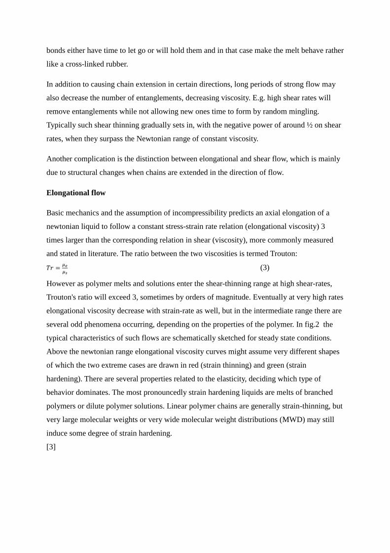
Elongational flow

Basic mechanics and the assumption of incompressibility predicts an axial elongation of a

newtonian liquid to follow a constant stress-strain rate relation (elongational viscosity) 3

times larger than the corresponding relation in shear (viscosity), more commonly measured

and stated in literature. The ratio between the two viscosities is termed Trouton:

(3)

However as polymer melts and solutions enter the shear-thinning range at high shear-rates,

Trouton's ratio will exceed 3, sometimes by orders of magnitude. Eventually at very high rates

elongational viscosity decrease with strain-rate as well, but in the intermediate range there are

several odd phenomena occurring, depending on the properties of the polymer. In fig.2 the

typical characteristics of such flows are schematically sketched for steady state conditions.

Above the newtonian range elongational viscosity curves might assume very different shapes

of which the two extreme cases are drawn in red (strain thinning) and green (strain

hardening). There are several properties related to the elasticity, deciding which type of

behavior dominates. The most pronouncedly strain hardening liquids are melts of branched

polymers or dilute polymer solutions. Linear polymer chains are generally strain-thinning, but

very large molecular weights or very wide molecular weight distributions (MWD) may still

induce some degree of strain hardening.

[3]

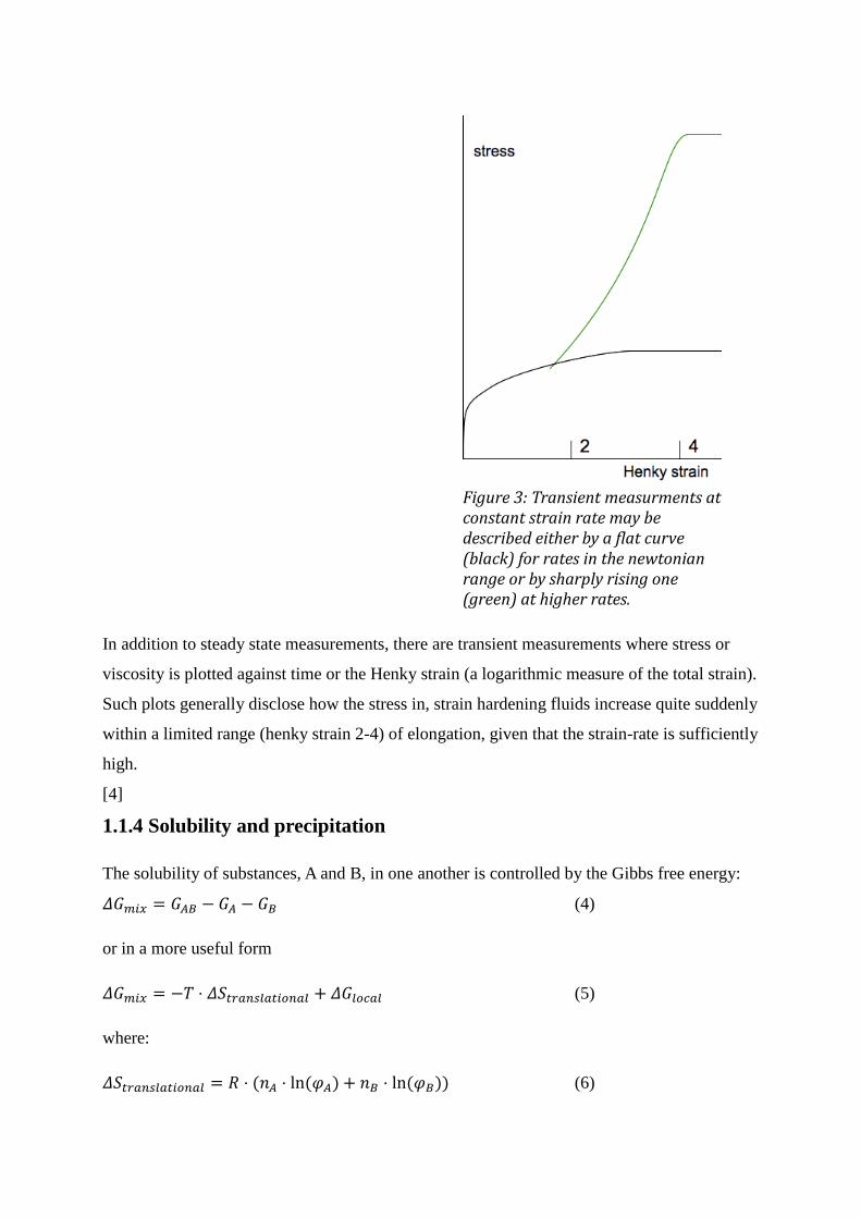
In addition to steady state measurements, there are transient measurements where stress or

viscosity is plotted against time or the Henky strain (a logarithmic measure of the total strain).

Such plots generally disclose how the stress in, strain hardening fluids increase quite suddenly

within a limited range (henky strain 2-4) of elongation, given that the strain-rate is sufficiently

high.

[4]

1.1.4 Solubility and precipitation

The solubility of substances, A and B, in one another is controlled by the Gibbs free energy:

(4)

or in a more useful form

(5)

where:

(6)

Figure 3: Transient measurments at constant strain rate may be described either by a flat curve (black) for rates in the newtonian range or by sharply rising one (green) at higher rates.

(7)

is the molar volume of monomer, is the respective volume ratio, is the number of

“independently distributed particles” and is the Flory-Huggins parameter describing

interaction between the different molecule species relative to self-interaction. Such interaction

is not completely enthalpic but may include entropic parts if e.g. polar molecules organize

their moment tangentially to a hydrophobic surface to minimize enthalpic contributions.

The term , “independently distributed particles”, is not its common name and is

intentionally used to cause curiosity, since it is quite arbitrary in the context of polymers.

Different parts of a macromolecule may move quite independently relative one another if

many monomer units are in between them, but more constrainedly if closer. If on the other

hand they are stiff, like a carbon nanotube, they will be completely locked. Thus nanotubes

are very difficult to dissolve, while chains of polyethylene are not, since is equal to the

number of polymers in the first case and closer to the much greater number of monomers in

the second. These considerations are central to cellulose, being a rather stiff polymer and

consequences are further discussed in the section on cellulose.

If studying the equations

above it is obvious that the

effect of will

dominate for low

concentrations of either

substance while is

more important in the middle

range, basically because there

is more potential interaction

then. Because as a

rule (although there are

exceptions) inhibits mixing,

there is typically a central

bulge in the curve,

creating two minima with

different optimal

Figure 4: Typical features of the Gibbs-free-energy-of-mixture curve for different ratios of a binary mixture.

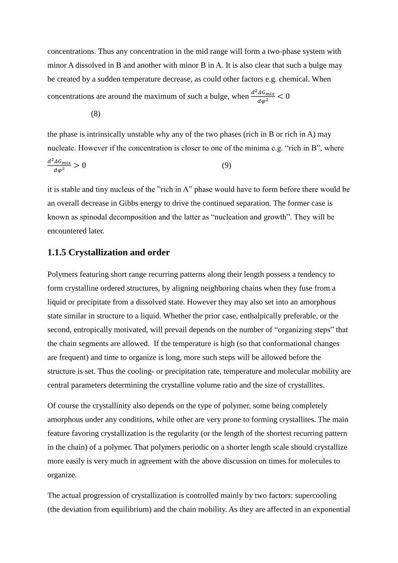
concentrations. Thus any concentration in the mid range will form a two-phase system with

minor A dissolved in B and another with minor B in A. It is also clear that such a bulge may

be created by a sudden temperature decrease, as could other factors e.g. chemical. When

concentrations are around the maximum of such a bulge, when

(8)

the phase is intrinsically unstable why any of the two phases (rich in B or rich in A) may

nucleate. However if the concentration is closer to one of the minima e.g. “rich in B”, where

(9)

it is stable and tiny nucleus of the ”rich in A” phase would have to form before there would be

an overall decrease in Gibbs energy to drive the continued separation. The former case is

known as spinodal decomposition and the latter as “nucleation and growth”. They will be

encountered later.

1.1.5 Crystallization and order

Polymers featuring short range recurring patterns along their length possess a tendency to

form crystalline ordered structures, by aligning neighboring chains when they fuse from a

liquid or precipitate from a dissolved state. However they may also set into an amorphous

state similar in structure to a liquid. Whether the prior case, enthalpically preferable, or the

second, entropically motivated, will prevail depends on the number of “organizing steps” that

the chain segments are allowed. If the temperature is high (so that conformational changes

are frequent) and time to organize is long, more such steps will be allowed before the

structure is set. Thus the cooling- or precipitation rate, temperature and molecular mobility are

central parameters determining the crystalline volume ratio and the size of crystallites.

Of course the crystallinity also depends on the type of polymer, some being completely

amorphous under any conditions, while other are very prone to forming crystallites. The main

feature favoring crystallization is the regularity (or the length of the shortest recurring pattern

in the chain) of a polymer. That polymers periodic on a shorter length scale should crystallize

more easily is very much in agreement with the above discussion on times for molecules to

organize.

The actual progression of crystallization is controlled mainly by two factors: supercooling

(the deviation from equilibrium) and the chain mobility. As they are affected in an exponential

fashion in opposite directions, there is a clear optimum temperature at which crystallization

will progress most quickly.

In most polymers crystalline spherulites, consisting of smaller plates, form. These plates are

created when polymers stack and fold, so that the plate thickness corresponds to the straight

sections between folds. The straight interior parts of any such platelet will have lower energy

than its surface where interaction is less optimized. Therefore the melting temperature is not

constant, but typically a function, of how well chains are aligned, ranging from that of a

perfect crystal to that of a completely amorphous sample. This is particularly interesting when

considering fibers, where orientation is induced by drawing, as the melting temperature could

then be raised. When studying such processes by small angle X-ray scattering it appears that

crystallization is starting in extremely many, very small regions and very quickly. As they

grow the crystallites start to encounter each other. The larger ones, who offer lower energy

states due to their size, will thus continually consume the smaller crystallites. This process

will not stop, but eventually becomes very slow when the intercrystallite surface volume

decreases as it is both the energetic driving force for and the interface through which the

process progresses. That is typically when crystallites are in the order of 10-8

-10-7

m.

1.1.6 Mesophases and orientation

In melts and solutions of polymers enthalpic driving forces may be strong enough to overtake

the entropic forces and cause molecules to self-assemble into structures of varying degrees of

order. Even though there are examples of both positional and multidirectional order in such

system, the interest to this work is limited to rigid polymers (like cellulose) forming nematic

mesophases, i.e. orientationally ordered. Their stability depending on the relative influence of

entropy and enthalpy, such phases are only stable below a certain temperature, termed the

clearing temperature, at which they become isotropic. Generally their stability range is also a

function of chain length and solute concentration.

1.2 Cellulose

The cellulose molecule consists of glucose units connected by covalent beta-(1,4) bonds

involving a 180° rotation, so that the actual repeat unit is composed of two mirrored glucose

units. Still the degree of polymerization, DP, generally refers to the number of glucose units

and not to the actual repeat units, which would be half that. In wood cellulose DP is typically

around 8000, while DP in pulp will have been reduced around 10 times by the pulping

process, varying quite much with the level of purity required.

In addition to the covalent carbon-oxygen bonds (among the strongest found in nature)

between glucose units, there are H-bonds involving hydroxyl groups (3 per glucose unit, at

carbons 2, 3 and 6) and the oxygen atoms. These can be both intermolecular (between

different neighboring chains) and intramolecular (between neighboring glucose units of the

same chain). When intramolecular they lock the conformation against rotation, which is how

any polymer would fold into new shapes. Thus the rather rod-like, stiff behavior of cellulose

molecules is explained. The intermolecular H-bonds are responsible for the, relatively to most

polymers, very strong interaction between chains. However there is also some Van-der-Waals

interaction adding to this.

Rotating the chain around an axis perpendicular to its length, it is not symmetric but has a

distinct direction, which is central when considering its crystal polymorphs, of which there are

several. Here however, only the two most common will be treated. Cellulose-I is found in

native cellulose, like wood, linen or cotton, while cellulose-II is the result when cellulose is

dissolved and precipitated.

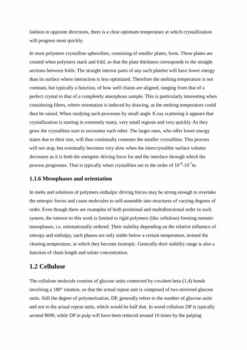
In cellulose-I (fig.5), chains are

parallel and bonded

intermolecularly by H-bonds,

laterally to sheaths, which are in

their turn stacked. In the stacking

direction Van-der-Waals bonding

is what holds the crystal together.

The upper limit for the stiffness of

an ideal sample of this structure

has been investigated experimentally and theoretically by several authors, finding E-modulus

values from 90 up to 220 GPa

along the chain and up to 15 GPa

perpendicular to it[5].

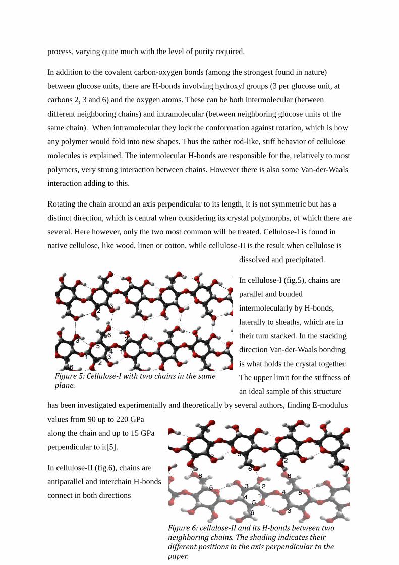
In cellulose-II (fig.6), chains are

antiparallel and interchain H-bonds

connect in both directions

Figure 6: cellulose-II and its H-bonds between two neighboring chains. The shading indicates their different positions in the axis perpendicular to the paper.

Figure 5: Cellulose-I with two chains in the same plane.

perpendicular to the c-axis. While cellulose-I has two intra- and one intermolecular H-bond

per glucose unit, cellulose-II instead has one and two respectively [6], which makes it less

stiff along the chain axis but probably less prone to chain sliding. For estimating the

theoretical strength of a material a simplistic, but common, model is to assume a 10% strain to

break for interatomic bonds, which means taking 10 percent of the E-modulus for a valid

measure. Thus the theoretical axial strength should be about 20 GPa for cellulose-I and

somewhere around 15 GPa for cellulose-II. However as will be observed later for Kevlar (as

is the case for many high-performance materials), the actual breaking strength obtainable in

real samples might be only 10% of that, due to stress raisers, interchain slipping and other

microscopic deviations from the ideal structure.

Both polymorphs tend to form fibrillar crystallites (for cellulose-I in wood, about 30 Å thick

and >5000 Å long), surrounded by amorphous regions. These regions might still be quite

directionally organized, why the decrease in density is often less than should be expected

from the amorphous volumetric ratio. That even the amorphous phases is rather ordered is not

surprising though, when considering its general tendency to crystallize to high volume ratios

(generally speaking, as ratios might vary a lot, depending on the rate and conditions). Water

and some other polar solvents swell cellulose, but it is a phenomena concentrated to the

amorphous regions.

Cellulose does not melt, but decomposes and eventually chars or burns at elevated

temperatures. Exposed to strong bases and acids in particular, it depolymerizes through

peeling and hydrolysis respectively. The former process proceeds only at one end of the chain

and is therefore most potent when chains are short and numerous. The latter case is an attack

on a linking oxygen atom. This will cleave chains at random positions, which is obviously the

most problematic for long chains. Both processes accelerate steeply with temperature, from

around 100°C and up. As all reactions involving cellulose they are active only in dissolved,

swollen or other amorphous material.

[1][7]

The physical properties of cellulose, e.g. high crystallinity, non-melting or its resistance to

dissolution are very much the results of abundant H-bonds and the inherent chain stiffness. It

can be argued from pure entropic considerations that a stiff rod would increase the number of

conformations (states), by freeing itself from fixation, only negligibly compared to what a

supple chain would. Thus a very significant amount of the “bonds” between sequel glucose

units would have to be stripped of both the two intramolecular H-bonds (freeing rotation), to

produce enough entropy gain, to make this micron-sized molecule move around fluidly. An

efficient solvent of such a polymer would thus probably have to interact with H-bonds

exothermally to function as such. E.g. the author has noted when mixing small amounts of

water with EmimAc, a potent cellulose solvent presented later, that it is obviously just that.

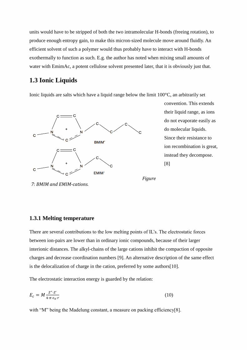
1.3 Ionic Liquids

Ionic liquids are salts which have a liquid range below the limit 100°C, an arbitrarily set

convention. This extends

their liquid range, as ions

do not evaporate easily as

do molecular liquids.

Since their resistance to

ion recombination is great,

instead they decompose.

[8]

1.3.1 Melting temperature

There are several contributions to the low melting points of IL’s. The electrostatic forces

between ion-pairs are lower than in ordinary ionic compounds, because of their larger

interionic distances. The alkyl-chains of the large cations inhibit the compaction of opposite

charges and decrease coordination numbers [9]. An alternative description of the same effect

is the delocalization of charge in the cation, preferred by some authors[10].

The electrostatic interaction energy is guarded by the relation:

-

(10)

with “M” being the Madelung constant, a measure on packing efficiency[8].

Figure 7: BMIM and EMIM-cations.

Making a very crude comparison with a simpler halide like NaCl (lattice energy slightly

below 800kJ/mol) could point to some interesting implications. Modeling BMIMCl as NaCl

but with ionic distances like those in BMIMCl (at least around twice that of NaCl [9]), thus

more than halving the lattice energy. [8] did essentially the same thing when they compared

sodium and Emim salts of various anions of different size (r=1,7-2,8Å) finding that melting

temperatures decreased from 801 to 185°C for the small (r=1,2Å) Na-ion and much less (87 to

7°C) for the larger (2-2,7Å, assymetric) Emim-ion. Such a tendency is consistent with the

mathematics predicting a stronger radius-dependence close to the singularity, i.e. for smaller

interionic distances.

Somewhat compensating for decreased electrostatic forces there can be hydrogen bonds,

especially in the case of halide-anions. Molecular numerical models of BMIMCl suggest that

these would be as large as 300-400 kJ/mol. [9]

This means that hydrogen and ionic bonds should be quite comparable in importance. The

hydrogen bond energies calculated by [9] are however much larger than ordinary H-bonds,

why such an imaginative compound as described above would still have much higher melting

point than ordinary H-bond dominated compounds like water or ammonia.

Another aspect of the enthalpy of fusion is the length of the alkyl-chains. While for short

lengths (n<10) they may cause steric hindrance and complicate packing, for longer chains a

further increase will make the IL behave more and more as an alkane with a charge in the end

rather than as an ionic substance. Thus Van der Waals forces will be increasingly abundant

compared to electrostatic forces, showing in a decreased melting temperature at first, but then

again increasing as for heavy alkanes. [10] For long (n>about 10) alkyl chain containing cat-

ions crystallization is increasingly impaired and there will be a glass-transition rather than a

distinct fusion point. Additionally aromatic structures may offer Pi-Pi interactions in crystals.

[8]

In collaboration with their low enthalpies of fusion, a high entropy difference between molten

and solid states also contributes to low melting points. The most explicit display of this is the

difference in melting temperatures between IL’s containing cat-ions with varying degrees of

symmetry, but with otherwise comparable structure. [8][ 9]Cat-ions with low degrees of

symmetry increase the number of available states much more upon melting than does one for

which several orientations correspond to the same state. Asymmetrical anions reasonably

influence in the same way. However the ones used in practice, are rarely large enough to

display as much asymmetry and there are fewer groups of similar anions but with varying

symmetry to make good comparisons possible.

1.3.2 Thermal stability

Thermal stability is limited by pyrolysis onset at 350°C of the organic cat-ions. Lower

decomposition temperatures are the result of nucleophilic anions (destabilizing the cation),

like the halides which are stable up to 250°C. However research on some compounds indicate

that long term stability may be about 50°C lower still.[8]

1.3.3 Viscosity

IL viscosities range from about 10 to 500 cPas. Small anions and any ability to hydrogen-

bond to cations give large viscosities. Thus halides distinguish themselves as viscous and

particularly chloride may raise viscosity in an exponential fashion, if present as an impurity,

e.g. left from synthesis. Most co-solvents have the opposite effect which may be described by

the equation:

(11)

: molar cosolvent concentration, : parameter typically around 0,2.

When considering the hygroscopicity of most ILs, it is quite evident that viscosity

measurements may vary a lot if extreme care is not taken to control moisture.[11]

Cations with long alkyl chains give higher viscosities than do shorter chains. When mixing

different species of IL’s, there can be sudden increases in viscosity at some threshold

concentration.

[8]

1.3.4 Polarity

Reichardt[12] has treated the subject of IL polarity rather rigorously, nuancing the concept of

polarity, often used to predict mutual solvation capacity and commonly expressed in the terms

of other parameters like: dielectric constants, dipole moments and refractive index. Rather he

would prefer a concept of “solvation power”, the consequence of the different types of

interaction between solute and solvent species: hydrogen bond donating/accepting tendency,

Van-der-Waals forces, permanent and induced dipoles, electron pair donating or accepting and

electrostatic forces. As a pertinent measure solvatochromic techniques (certain molecules,

displaying charge separation, have light emission, whose wavelength is dependent on the

electrochemical surroundings) can characterize the sum of most of such interactions

(however not all, e.g. not electron pair accepting and hydrogen bond accepting). He found that

most IL species were found somewhere between acetone and water on this solvatochromic

index scale. A central aspect was H-bond donating capacity of the cation, which is dependent

on available hydrogen atoms close to the location of electric charge. This would be why

1,3alkylimidazoleum and monoalkyl ammonium salts have higher indexes than their more

fully alkylated relatives. This aspect proves more relevant than e.g. charge separation, which

would place IL’s at one extreme of the scale. It is clear that even though charge separation is

greater than in molecular compounds with separated charges (zwitterionic and dipolar), the

difference will not be that important since opposite charges will still stay close in the

condensed state.

Specifically the important groups of species for cellulose dissolution: 1,3alkylimidazoleum

salts were found in the range of the simplest alcohols, not fully alkylated ammonium salts;

between methanol and water and pyridinium salts; spanning from acetone to water.

1.3.5 surface tension

Law et al. [13] measured surface tension for several combinations of n-Mim cations (n=4, 8

and 12) with some common anions and found values ranging from 24-47 mN/m at ambient

temperatures. The decline with temperature was around 0,04-0,08 mN/m per °K. Increasing

alkyl chain length impacted negatively on surface tension while large anions had the opposite

effect.

1.3.6 In a cellulose context

1.3.6.1 Generalities

IL solvents for cellulose dissolution generally combine a species of imidazolium, ammonium

or pyridinium cation, with a chloride, acetate or formate anion. Particularly the 1-alkyl-3-

methylimidazolium salts of chloride and acetate (EMIMAc, BMIMCl) are the most frequently

studied in cellulose spinning trials and related research. [9]

Desired properties when combining ion species are low melting point, viscosity and surface

tension in addition to efficient cellulose dissolution, low degradation of DP, low toxicity, easy

solvent recycling, little corrosiveness and simple coagulation methods, which together shall

result in good economics.[14]

In practice it turns out that there are tradeoffs between these properties. E.g. high viscosity

might either make a dissolution process infinitely slow or require elevated temperatures

prohibited by their consequent decrease of cellulose-DP.[15] Thus a very high theoretical limit

of dissolved cellulose concentration may be practically unattainable. As IL’s have very low

vapor pressures it is their thermal decomposition temperature that limits the range of use.

However, they are generally above 250°C which is anyway avoided by a large margin, for the

sake of preserving the polymer DP.

Another issue is the precipitation bath, which should preferentially be nontoxic, not too

volatile and give good fiber properties, without much residual solvent or excessive dwell

times. The bath media must also be easily separable from the IL to facilitate solvent recycling.

However, water, alcohols and mixes thereof generally make good alternatives, leaving the

dissolution process as the major concern.

1.3.6.2 Reported trials of spinning cellulose-IL solutions

Kosan et al.[16] performed spinning trials for EMIM and BMIM chlorides and acetates as

well as NMMO in a falling jet, water coagulation bath. They spun through spinnerets with 90

or 100 diameter holes at temperatures ranging from 90-116°C and obtained fibers around 1,5

dTex with tenacities from about 45-55 cN/Tex. The chlorides produced the most viscous

dopes which was stated as the reason for those fibers being the strongest. The initial DP of

569 decreased to around 500 over the quick dissolution-regeneration cycle. Air gaps were

varied between 40 and 80 mm and their draw ratios around 5(aproximately calculated from

their data, as it was not available in the original article).

Cai et al. [17]spun BMIMCl-cellulose (8wt%) solutions and compared them to the NMMO-

cellulose solutions (10wt%) spun by Zhang et al. [18] with the same equipment (no falling jet,

water bath, 50mm air gap, through 145 and 80 diameter holes). Their obtained data for

BMIMCl spun fibers with draw-ratios 2,4 and 3,5 with the coarser spinneret is summarized in

table 1.

Draw-ratio Crystallinity

(%)

Birefringence Tenacity

(cN/Tex)

Initial

modulus

Elongation

(%)

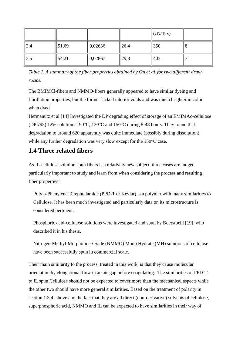
(cN/Tex)

2,4 51,69 0,02636 26,4 350 8

3,5 54,21 0,02867 29,3 403 7

Table 1: A summary of the fiber properties obtained by Cai et al. for two different draw-

ratios.

The BMIMCl-fibers and NMMO-fibers generally appeared to have similar dyeing and

fibrillation properties, but the former lacked interior voids and was much brighter in color

when dyed.

Hermanutz et al.[14] Investigated the DP degrading effect of storage of an EMIMAc-cellulose

(DP 795) 12% solution at 90°C, 120°C and 150°C during 8-48 hours. They found that

degradation to around 620 apparently was quite immediate (possibly during dissolution),

while any further degradation was very slow except for the 150°C case.

1.4 Three related fibers

As IL-cellulose solution spun fibers is a relatively new subject, three cases are judged

particularly important to study and learn from when considering the process and resulting

fiber properties:

Poly p-Phenylene Terephtalamide (PPD-T or Kevlar) is a polymer with many similarities to

Cellulose. It has been much investigated and particularly data on its microstructure is

considered pertinent.

Phosphoric acid-cellulose solutions were investigated and spun by Boerstoehl [19], who

described it in his thesis.

Nitrogen-Methyl-Morpholine-Oxide (NMMO) Mono Hydrate (MH) solutions of cellulose

have been successfully spun in commercial scale.

Their main similarity to the process, treated in this work, is that they cause molecular

orientation by elongational flow in an air-gap before coagulating. The similarities of PPD-T

to IL spun Cellulose should not be expected to cover more than the mechanical aspects while

the other two should have more general similarities. Based on the treatment of polarity in

section 1.3.4. above and the fact that they are all direct (non-derivative) solvents of cellulose,

superphosphoric acid, NMMO and IL can be expected to have similarities in their way of

coagulating.

1.4.1 Lessons from Kevlar

Kevlar tenacity is commonly about 2-3 GPa, its modulus 50-150 GPa and elongation-to-break

2-4%. As with most high performance fibers, there are conflicting objectives with high

strength, toughness and elongation on one hand and high modulus on the other. This whole

section is based on H.H. Yang’s book [20] on the subject.

1.4.1.1 Some justification for the comparison

Like cellulose, Kevlar is stiff and dominated by intermolecular hydrogen bonds and carbon

ring structures although aromatic instead of sacharide type. Due to the hydrogen bonds it

melts only at very high temperatures (where even the aromatic Kevlar starts to degrade), as

would cellulose if it would not char at far lower temperatures. Therefore the problem of DP

degradation when dry spinning has forced the development of air-gap wet spinning, with

anhydrous sulfuric acid as solvent. Kevlar is also quite hydrophilic and ties some percent of

moisture from the air, that requires heating for its removal. Additionally both Kevlar and

cellulose solutions have been reported to display liquid crystalline type behavior over certain

concentrations of solute.

Thus we will advance along the hypothesis that the type of rupture, defects causing rupture,

fiber microstructure, fiber properties like brittleness and the impact of crystallinity and DP

will bear many similarities between the two types of polymer from the mechanical viewpoint;

obviously the validity of such comparisons does not cover the more chemical aspects like

degradation temperatures or useful solvents.

Useful facts about Kevlar

Birefringence (the difference in refractive index in axial and radial direction) is an interesting

measure for orientational order.

Kevlar is relatively creep resistant due to high crystallinity and glass temperature, but does

still creep, especially at higher stresses and temperatures and when wet. It is reasonable to

expect similar behavior from IL cellulose fibers.

Kevlar is sensitive to torsion, which causes shear forces, splitting filaments lengthwise and

thus weakening it also to a later tension. While its shear modulus still compares well to other

fibers in absolute terms its ratio of tension-to-shear modulus is much larger.

Another display of the weaker perpendicular cohesion is its tendency like lyocell, to fibrillate

severely when exposed to abrasion. Further this will also show in flexural bending tests,

where initially fibrillation occurs very rapidly due to its stiffness, but which then will not

continue to weaken the fiber, which still makes it quite well processable.

1.4.1.2 Structure and morphology

Kevlar fibers are typically composed of a dense skin with very high axial orientation but

lower crystallinity, about 500-2000 nm thick and a very crystalline core. The skin is axially

continuous making it very strong, but not as stiff due to the lower crystallinity, while the

crystalline core is stiffer but not as homogeneous due to the axial joints of lower density

between the sequel crystallites, each about 50 nm long and 5 nm thick. These crystallites in

the core are arranged in a radially symmetric fashion. The overall crystallinity of the fiber has

been reported within a relatively wide range (70-95%), depending both on author and type of

Kevlar fiber.

Heat treatments up to 400°C have proved able to recrystallize the structure and increase

crystallite size, leading to higher modulus.

Upon assumptions of bond strengths, bond densities and an ideal structure, theoretical limits

for tenacity and modulus have been estimated to 21,7 and 238 GPa respectively. However

assuming the possibility of slip yielded tenacities at 5,3 GPa, which is forcibly a quite

arbitrary number due to the dependence on DP, that must enter any such calculation. The

discrepancy between theoretical and measured modulus (70-80%) is largely blamed on the

non-crystalline portion and to lesser extent on chains’ non-ideal axial alignment. Tenacity is

much more complex to explain.

1.4.1.3 Ruptures

There are three frequent kinds of failures in Kevlar fibers:

-Tapered rupture occur at lower strain rates and may decrease the diameter by as much as 5

times before rupture. Such necking down is generally an indicator of a well processed fiber

that uses a large fraction of the theoretical potential of the material.

-Fractured and fibrillated break is the most common mode of rupture for Kevlar. Some

necking will show on the split fibrils, which have been separated laterally before rupturing

one after another. It is generally not a witness of the same strength as the prior, but still good.

- Kink bands are faults of chain disalignment, which may cause rupture at low stresses. No

necking is seen and the rupture surface is normally at roughly 60° to the fiber axis.

One theory for explaining rupture in Kevlar assumes that cracks commence in the fiber

surface and propagate through the skin at a small angle to the axis and then through the core

intermittently through and across microfibrils to connect with another surface flaw, which

could be found at some distance along the fiber.

1.4.2 Mono/poly-phosphoric acid

Considerable research has looked to spin high tenacity fibers from cellulose solutions in

anhydrous phosphoric acid and mixtures with other acids like formic acid.

Phosphoric acid H3PO4 can equally be described as a 3:1 mixture of H2O and P2O5. This ratio

may be varied continuously each corresponding to well defined balances between water,

orthophosphoric and various oligophosphoric acids. Phosphoric acid tend to polymerize into

longer chains of acid at high concentrations.

The cellulose dissolving capacity is very sensitive to these balances (there is an optimal

concentration around 72-76 wt% P2O5). As in most cellulose dissolving systems, water may

substitute for the OH-groups of cellulose, giving its presence a very negative effect on

dissolution. To explain the opposite, quite surprising, problem of too little water, Zhengou et

al. [21] have proposed that larger polymers of phosphoric acid (present at low concentrations

of water) are less mobile than monomers and will neither brake more hydrogen bonds in the

structure, than does a monomer, which would explain this phenomenon.

Cellulose may be dissolved up to 38% by weight and anisotropy occurs from around 8%.[21]

Mesophases are obtained over a range of cellulose concentrations up to the corresponding

clearing temperatures, which increase with P2O5/H2O ratio and DP. Particularly, free water

and the low-DP fractions (below the persistence length) of cellulose in the solution have

strong negative impact on clearing temperatures.

Degradation can be severe if temperatures are not controlled, but typical values during a

dissolution-spinning-regeneration cycle would be around 25% for an initial DP of 800, since

dissolution is very quick (in the range hours to minutes), thus reducing exposure times.

Some fibers produced by Boerstoehl had very high tenacities (1,7 GPa) and modulus (45 GPa)

and crystallinity around 50%. These were similar to Kevlar in that they had very limited

damping over wide temperature ranges. While stress-strain curves for Kevlar show an

increase from the initial elastic modulus, these fibers were more similar to other types of

cellulose fibers as their curve had a quite distinct knee around 0,5-1% strain, where some kind

of yielding behavior appeared to set in, causing a constant modulus until rupture at 6% strain.

However the modulus decreased much less than it does for various kinds of viscose with or

without post drawing.

These are among the strongest cellulose fibers reported and the only drawback seems to be

that they were produced by coagulation in acetone, which was problematic from a feasibility

perspective. [22]

[19]

1.4.3 NMMO-Lyocell

NMMO MH is a direct solvent for cellulose that has been in commercial use since the 1980’s.

As the pure NMMO is too high melting (180°C) its hydrate is used instead. However, as with

most solvents for cellulose, there must not be too much water since it inhibits cellulose

dissolution. Often the molar ratio (generally referred to as the hydration number “n”) of

around 0,7 H20/NMMO is used where mesophases may occur at concentrations above 12%

cellulose (DP 670, 110°C). When n approaches 1 and particularly as it goes above, dissolution

capacity goes down, spinnability becomes very bad and mesophases are out of the question.

DP-values do affect solubility but generally is not a problem up to a DP of 1000, which

includes most dissolving pulps. [23]

Kosan et al. [24] used a lower DP (367) and detected mesophases from 16.5 wt% cellulose

with clearing temperature 75-80°C and 95-100°C for 20,4 wt%.

Completely anhydrous NMMO should dissolve up to 35 wt% [25], while tracing of diffusion

coefficients for monohydrate predicts the presence of non-dissolved material already at 15

wt% [26][27].

1.4.3.1 The dope

Liu et al. [28] has studied phase transitions in NMMO-water-cellulose melt. With increased

cellulose concentrations, the solution melting temperature decreased and their overall

behavior was increasingly that of an amorphous material, the melting point being more

diffuse when heating and (with concentrations 6% and less) displayed a relatively sudden

fusion point, delayed by some 30-60°K when cooling at 1°K/min. For higher concentrations

the polymer chains posed such a hindrance to crystallization that no phase transition was

observed within the positive temperature range studied. However Biganska and Navard [29]

presented a slightly different picture, of phase separation where crystalline NMMO

surrounded the cellulose phase, even at high concentrations of cellulose. Regrettably neither

Liu et al. nor Biganska-Navard present their exact hydration numbers, which probably

explains their different findings. Laity et. al. [26] (working with hydration numbers slightly

above 1) agrees with Biganska-Navard, but states that there is still some rather strong

cellulose-NMMO interaction.

Further, Liu et al. found that enthalpies of fusion and heat capacities decrease (more than

could be explained by simple differences in the respective values for the pure constituent

species and weight ratios), when cellulose concentrations increase.

As expected, they also found densities to increase linearly (except for some irregularities

around 2-6wt%, see fig.x) with cellulose weight ratio . E.g. at 30°C and 100°C according to

respectively: (12)

and (deduced from their data). (13)

If assuming that: at relatively low concentrations the densities would depend on the volume

ratios and densities of the pure substances, like it does if mixing two immiscible phases, thus

according to the equation:

(14)

the apparent density of cellulose would be around 2,3 (much larger than 1,62 for crystalline

cellulose-II), which indicates a very strong interaction between NMMO and cellulose.

Dissolution can be performed with an excess amount of water and some additional passive

organic non-solvent to decrease viscosity while mixing and homogenizing the solution. The

excess water and the filler non-solvent are then evaporated to achieve a fully viscous dope.

[30]

1.4.3.2 Spinning

Spinning is performed with air-gap, allowing large draw-ratios and good orientation, into a

water bath.

A particularity of hydrated spinning dopes like NMMO-MH (as opposed to an IL-dope) is the

possibility of a cooling effect due to evaporation if the air gap is very dry. Cooling through

evaporation is often much quicker than through conduction in air. However it appears that no

investigation treating it in particular, has been reported in the literature.

Mortimer and Peguy [31] observed that a certain set of draw ratio, viscosity, line speed,

solution temperature and air-gap climate generated a natural strain distance over which it

would produce most of the strain even with much longer air-gaps (i.e. solidify, more or less).

However if the air-gap was shorter than this natural distance, the strain had to be completed

within a much shorter distance, which would produce a rather constant looking acceleration

compared to the exponentially decreasing acceleration in the unforced case. In forced cases

there was no dye swell. The drawing distance decreased with dryer and cooler air-gap climate.

E.g. 100% relative humidity and 30°C increased the draw length from 5 to 50 mm, compared

to 2% relative humidity and 0°C.

The general conclusion from their work would be that air-gap spinning in some cases is a

process very similar to melt-spinning.

Mortimer and Peguy [31] also measured birefringence in-line during spinning. They found

that when spinning with efficient cooling, birefringence did not increase linearly with the

dimensionless velocity as thicker (i.e. less well cooled) fibers did. As the more efficiently

cooled fibers’ birefringence increased more initially than later on, they drew the conclusion

that when drawing was performed at temperatures below the crystallization temperature,

inhibiting relaxations, chains might become fully extended and allow fiber yielding through

chain slippage. These fibers had coinciding birefringence-dimensionless velocity curves for

different air gaps, while the thicker fibers display sharper rises in birefringence as air gaps

were lengthened, meaning better cooling.

When testing air gap climates, they found that the birefringence increase was concentrated to

the latter parts of the dimensionless velocity domain in a dry and cool atmosphere, with a

quite sharp rise in the very end (both for 20 and 250 mm air gaps). It should however not be

forgotten that this corresponds to a much more extended portion of the flow, when considered

on the time line rather than the dimensionless velocity (for 250 mm).

In a warm and humid air gap, birefringence started off at a much lower level, but then rose

quickly. Towards the end of the dimensionless velocity span however, it began to flatten for

the longer air gaps. A 250 mm air gap even featured decreasing birefringence in the latter part

where drawing was no longer ongoing, which was attributed to hygroscopic accumulation of

water from the surrounding air, in the fiber, which decreased its viscosity and consequently

accelerated molecular relaxations.

1.4.3.3 Coagulation

Coagulation progresses through diffusion of water and NMMO, in opposite directions (24).

Biganska et al. [27][29] have looked into this process in discs (however not in fibers) and

determined diffusion coefficients in the order of 10-9

and 10-10

for water and NMMO

respectively, which further decreased by a factor around 40 (for water) and 20 (NMMO),

when the bath was substituted with one containing 50% NMMO. Such displayed nonlinearity,

stems from the water content’s positive effect on diffusion, which was also confirmed by

Laity et al. [26].

They concluded that water would first swell the structure before significant amounts of

NMMO could diffuse out. DP did not affect diffusion. Increased cellulose concentrations, on

the other hand, did slow the diffusion of NMMO, but not that of water. The main reasons for

these differences are two: the diffusion’s dependence on free volume as predicted by Yasuda’s

theory [33], implying that molecule size will have exponential influence along with the

chemical affinity to the polymer, which are both obviously much larger for NMMO, making it

slower.

Laity et al. also applied general theories of polymer dissolution to the ternary phase diagram

of cellulose-NMMO-water, recognizing four main possible modes of precipitation:

– case1, vitrification: increasing cellulose concentration, due to NMMO diffusing

out, ending in an amorphous gel.

– case 2, nucleation and growth of liquid phase pores: water concentrations rising

simultaneously with those of cellulose forces separation, as the solvent capacity deteriorates.

This gives a continuous morphology with intermittent solvent pores, wherefrom the solvent

will be quite slow to diffuse out.

– case 3, spinodal decomposition: when water, diffusing in, balances NMMO

diffusing out, to cause instability between liquid and solid nucleus formation, set off in either

direction by local deviations from the equilibrium composition gradually amplifying via a

liquid-liquid phase separation, shaping a wormlike pattern of pores and cellulose.

– case 4, nucleation and growth of solid crystallites: when water diffusion

dominates, chains of cellulose will be abandoned by the NMMO molecules and readily

adhering to the nearest neighboring chain, they form crystallites surrounded by a liquid phase

of diluted solvent.

From Laity et al.’s investigation by magnetic resonance imaging into coagulating surfaces

over time, it is clear that the bath-solution interface is very different from the bulk of the

solution. When the skin forms, NMMO is diffused out fast enough to generate something like

“case 1”, as there is no viscous solution to diffuse through (analogous to an electrical

resistance). Biganska et al. [29] observed “case 1”-like, dense and non-porous structures,

when fused solution samples were coagulated, displaying a sharp precipitation front.

Centrally though, very little happens to NMMO levels before the water concentration has

doubled there (and most importantly increased much more, further out), at which time the

NMMO concentration starts its rather exponential looking decline. [26] Thus there is a good

case for the spinodal coagulation mode or possibly even the “case 4” above. Mortimer and

Peguy [31][34] and others [26][29] suggest that spinodal decomposition is the valid mode for

the core when NMMO-cellulose solutions coagulate in water.

This is in accordance with observations by SEM of fibers spun into water with extremely thin

amorphous skins and more porous and crystalline interiors, which show structural variations

with a longer periodicity. [35]

It is a reasonable supposition, that crystallinity should increase according to

vitrification<”case 2”<spinodal<”case 4”, since mobility and time are required for molecules

to reorganize into crystalline phases. This gains support from the observations by Fink et al.

[35] who compared coagulation in a series of the lightest simple alcohols to water. The slower

dynamics of the larger alcohol molecules and the consequently less violent coagulation gave

very distinct skin-core structures and much lower crystallinity. With 2-Propanol there was a

thick, dense amorphous skin, containing a thin porous center, which displayed a combination

of decreased proneness to fibrillate, while still maintaining good tensile properties.

Coagulating in 2-Butanol or Hexanol gave much larger pores while crystallinity decreased

further, producing a fiber with bad tensile performance. 2-Butanol even had worse fibrillation,

while Hexanol displayed good resistance. Ethanol was quite similar to water. By employing a

two phase coagulation bath, with a gap of Pentanol topping a water column, they managed to

retain most of the good from each type of non-solvent as the Pentanol probably did not find its

way into the core before the water did, but could still affect the skin positively.

1.4.3.4 Structure

Crystallinity is generally quite high with NMMO and a range of results have been reported

e.g.: 25% with Hexanol [35]; 42% [35] and 44% [36] in water.

Crystallites are 3,5-5,5 nm wide and sometimes as long as 45 nm and their cross sections are

quite circular.[35]

Fiber birefringence has been reported around 0,04 in commercial staple fiber [36], but [23]

showed that lowering hydration number “n” or increasing concentration or DP, affected

birefringence positively for large draw ratios ( for , and

DP=960) as can be expected. It is not just the crystalline parts that are directionally ordered;

even the amorphous parts carry this trait and thus add to birefringence [35].

Fractured surfaces of NMMO fibers resemble a kind of pullout of rather long fibrils [35],

witnessing of the poor interfibrillar shear strength, that allows week points of neighboring

fibrils to add to the same rupture even when longitudinally quite distant.

1.4.3.5 Fibrillation

Fibers suffer severe fibrillation, which is attributed to their high crystallinity and chain

orientation, meaning few chains linking crystallites and fibrils laterally. Thus birefringence,

low hydration numbers, high draw ratios and cellulose concentrations tend to increase

fibrillation. Longer air gaps or higher concentrations of NMMO in the bath have been shown

to lessen fibrillation. Fibers are also more sensitive in the wet state, due to interfibrillar voids,

which tend to fill up with water, weakening the lateral cohesion.[32][37]

Considering causes on the microscopic scale, spinodal decomposition is to blame, as typically

very few chains penetrate the liquid phase, which will collapse during drying, to form the

interfibrillar volume in the final fiber structure.[33]

1.5 Summary of basic flow theory

1.5.1 Shear flow in die

Inside long capillaries shear is the dominant force resisting the extruding pressure for

Newtonian liquids. It relates to the flows according to:

(15)

The differential equation for momentum:

, (16)

governs a constant and fully developed laminar flow in a pipe. [38]

Several useful expressions for Newtonian fluids can then be derived, by solving with

boundary conditions:

and

, generating:

-

(17)

before integrating over the pipe cross section to deduce the flowrate:

(18)

or as is often of intrest the viscous pressure drop can be deduced by multiplying both sides of

eq.19 with the capillary length.

(19)

If instead derivating the solution with respect to the radius, the shear-stress can be deduced:

(20)

or

(21)

However, as explained in 1.1.3, polymer solutions, unlike Newtonian fluids, have shear

thinning viscosities and viscoelastic behavior at high shear rates. Typically their shear

viscosity is described with a power-law: (22)

Then shear will concentrate to a lubricating layer close to the capillary wall, while a central

plug passes through the die without much deformation. For liquids described by a power-law

as in eq.22 this effect can be corrected by an analytically generated “Rabinovitch correction”:

(23)

which is introduced in expressions like eq.24

(24)

Its terms can rearranged to yield:

(25)

Gradual narrowing (a typical geometry for dies) can be calculated by integrating eq.25 along

the flow (z) axis, with R as a function of z, which gives reasonable approximations.

More complex to calculate are the contributions to the flow resistance generated by the transit

portion between reservoir and capillary. There the elongational viscosity, the delayed

development of the flow profile and shear from the flow directly upstream of the die. These

will convert some of the pressure to heat and some to mechanical tensions. This may be

significant and is best investigated by capillary rheometry and Bagley plots.

[39]

1.5.2 Elongational flow in airgap

The author (as have some others treating airgap-wet spinning[28]) judges the most pertinent

literature available to be that describing traditional melt spinning. Therefore “High-speed

fiber spinning” by Ziabicki et al. [40], a bible on the subject, was used to gather the most

useful parts of the theory on this subject. This section is based on that work, where no other

reference is cited.

Drawing the fiber means, to gradually accelerate it from the extrusion velocity to the take up

velocity, which forcibly must happen over the part of the spin line where the dope is still

flowing, i.e. before the coagulation bath.

The line tension is the significant accelerating force on any section of fiber, which causes the

elongational flow guarded by the relation:

(26)

When this relation is combined with

(27)

the result is a differential equation:

(28)

Its solution is simple:

(29)

with

or

(30),(31)

From eq.30,31 at its take up speed and reorganizing the terms yields:

(32)

However the appearingly simple term

in eq.32 is actually

in most real

cases.

To complicate matters even further there are additional forces, particularly at high speed,

which integrate over the drawing length, causing a variation in tension throughout the air-gap.

Air-drag on the fiber surface and inertial pull increase tension towards the end, while on the

contrary, gravity redistributes tension towards the domain closer to the die. The total is

guarded by the complete momentum equation:

(33)

This is obviously a task for computers to handle, but to know the underlying equation and its

various terms can be useful in a rule-of-thumb-like approach.

Air drag force: (34)

The expression for drag force per surface unit appears simple:

(35)

However determining the friction coefficient, , requires experimental fitting to relate it to

the Reynolds number,

(where is the kinematic viscosity of the surrounding fluid

air), for its determination, which conveniently other researchers already have done, to yield:

(36)

( and )

Thus the resulting drag force on an incremental length of the filament will be:

(37)

which is obviously dominated by the line speed, with only very slight dependence on the

radius. For a set die diameter, i.e.

, it is of course possible to express it as a function

only dependent on and the constant flow, :

(38)

Surface tension:

(39)

In small dimensions surface tension acts on a liquid jet somewhat like the membrane of a very

long rubber balloon filled with liquid. It will simultaneously cause a tangential stress, acting

to reduce the diameter and an axial stress acting to increase it. The net nominal axial stress

from these effects is:

(40)

There is also a hydrostatic stress generated by the surface tension:

(41)

As it decreases with the jet radius, the will be much higher for thin portions, why

the surface tension acts to amplify any variations in thickness, ultimately forming droplets.

[41]

returning to eq.39 found in Ziabicki's choice of differential equation, it is simply eq.40

multiplied with the cross-sectional area, , to express the surface tension addition line

tension force, which is then differentiated, it being the impulse equation. However Ziabicki

states that it is generally unimportant, unless the melt or solution is very low in viscosity.

Draw resonance and line rupture

When a fiber section is drawn and its diameter decreased, the line tension is spread over a

smaller area and the stress consequently increases. Thus if any local stochastic variation in

diameter is not to self-amplify uncontrollably, there must be phenomena countering this, by

increasing the viscosity. Cooling rates increasing with decreasing diameters and elasticity

(long relaxation times) are such. High viscosities are also beneficial while inertia and surface

tension tend to worsen resonance. Resonance is therefore most important at lower speeds and

high draw ratios.

From the above it would seem beneficial with high elasticity, elongation thickening and high

viscosities. However such a dope would instead build up too intense stresses, causing a

sudden rupture, when its critical elongation rate is surpassed.

To reduce this type of problem, e.g. speed could be decreased or temperature and drawing

length could be increased.

Cooling

As temperature along with elongation rate, are the controlling factors for the elongational

viscosity, the fiber cooling is one of the most interesting processes in any melt- or air-gap

spinning process. Heat dissipates through conduction to the surrounding air and by radiation

(and by evaporation in case there is volatile solvent in the dope), but it may also be produced

by viscous conversion of mechanical into thermal energy or by phase-transitions. However

only conduction, radiation and viscous contributions are worth consideration in air-gap spun

fibers from ILs.

Radiation is controlled by Boltzman’s law: (42)

which gives an expression for radiative cooling per unit fiber length:

(43)

The complication is the emissivity coefficient , which even though fluids generally absorb

and emit well in the infrared range might be quite different from 1 (a black body), since the

filament is so thin that it might transmit some of it, possibly making it more appropriate to

consider the radiating volume, rather than the surface. [42] showed that PP and PB fibers,

closely below their melting temperatures had emissivities in the range 0,2-0,3 for diameters

around 100 , but steeply decreasing indicating that values could be around 0,1-0,05 for

typical final fiber diameters of 10-20 mu. Translating such numbers to this work is forcibly of

very approximate nature, as a solution spun, being fluid, should reasonably have more

available energy levels, providing more radiative interaction and consequently higher

emissivities.

Another aspect of this partial IR translucency is that radiative cooling will not have the same

stabilizing effect on fiber resonance as e.g. conduction, which is controlled by a surface-to-

volume ratio and thus strongly affected by fiber radius. However if the pertinent region is

close to the die, the fiber might still be thick enough for radiative cooling to give some

damping effect.

Entering typical values into the above stated formula reveals radiative heat transfer

coefficients below 1W/m2K.

The conduction depends strongly on the boundary layer closest to the fiber. The whole

temperature difference between fiber and the air will be concentrated over this layer, giving a

very steep gradient. To calculate it, could by itself be the subject of a much wider work than

this one. However there are some approximations derived from experiment. The general

formula for conductive heat flow per unit length, from a cylindrical surface:

(44)

can be applied with an derived from expression of the Nusselt number:

(45)

where

(46)

Combining eq.45 and eq.46 gives eq.47:

(47)

Even if not attempting quantitative use of these formulas, a useful relation to remember is that

for a set draw ratio, a moving line segment will cool according to:

(48)

It is also possible to approximate the range of the temperature difference between skin and

core. This is generally assumed to be negligible, but can actually be of the order 10 °K

(gradient around 1 °K/mu), for very high speeds.

This kind of treatment does neither deal with cross flow, which might further diverge model

from reality.

For take up speeds between 1 and 10 km/min Ziabicki stated heat transfer coefficients in the

range of 1-2 kW/m2K, making it a thousand times more important than radiation, explaining

why he did not go through the trouble of describing that.

Viscous heating

The dissipation of mechanic energy to thermal in flows is typically expressed as:

[43], (49)

which in steady flows is equivalent to:

(50)

However in an elastic fluid such as a polymer melt or solution, eq.50 would only be accurate

when the flow has stabilized. Meanwhile during an initial transient stage of straining, much of

the deformation energy described by eq.49 would be stored elastically. How much, is a

complicated matter to expand on, but for making a guess it might be useful to look at ratios

between loss and storage modulus of oscillatory shear at a frequency corresponding to the

timescale of the flow.

2 Practical work

The practical work of this thesis, initiating development of air-gap spinning techniques of

cellulose-IL dopes, at Swerea IVF’s fiber section, consisted of several steps:

- designing and constructing a falling-jet bath, with a constant water level and

incorporating it with the present wet-spinning equipment.

- Dissolving the polymer in the chosen IL-solvent (EmimAc), investigate its

properties and refining the method to obtain a spinnable dope.

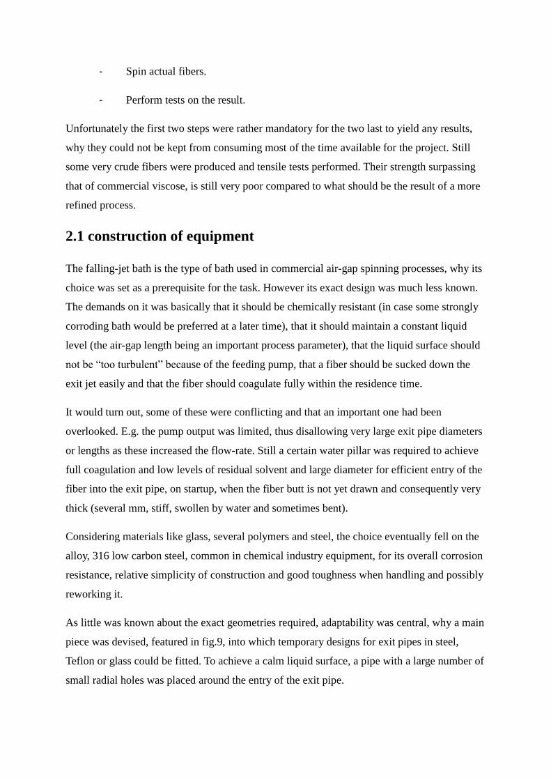
- Spin actual fibers.

- Perform tests on the result.

Unfortunately the first two steps were rather mandatory for the two last to yield any results,

why they could not be kept from consuming most of the time available for the project. Still

some very crude fibers were produced and tensile tests performed. Their strength surpassing

that of commercial viscose, is still very poor compared to what should be the result of a more

refined process.

2.1 construction of equipment

The falling-jet bath is the type of bath used in commercial air-gap spinning processes, why its

choice was set as a prerequisite for the task. However its exact design was much less known.

The demands on it was basically that it should be chemically resistant (in case some strongly

corroding bath would be preferred at a later time), that it should maintain a constant liquid

level (the air-gap length being an important process parameter), that the liquid surface should

not be “too turbulent” because of the feeding pump, that a fiber should be sucked down the

exit jet easily and that the fiber should coagulate fully within the residence time.

It would turn out, some of these were conflicting and that an important one had been

overlooked. E.g. the pump output was limited, thus disallowing very large exit pipe diameters

or lengths as these increased the flow-rate. Still a certain water pillar was required to achieve

full coagulation and low levels of residual solvent and large diameter for efficient entry of the

fiber into the exit pipe, on startup, when the fiber butt is not yet drawn and consequently very

thick (several mm, stiff, swollen by water and sometimes bent).

Considering materials like glass, several polymers and steel, the choice eventually fell on the

alloy, 316 low carbon steel, common in chemical industry equipment, for its overall corrosion

resistance, relative simplicity of construction and good toughness when handling and possibly

reworking it.

As little was known about the exact geometries required, adaptability was central, why a main

piece was devised, featured in fig.9, into which temporary designs for exit pipes in steel,

Teflon or glass could be fitted. To achieve a calm liquid surface, a pipe with a large number of

small radial holes was placed around the entry of the exit pipe.

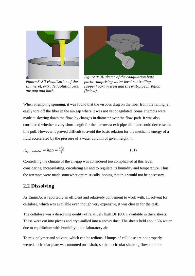
When attempting spinning, it was found that the viscous drag on the fiber from the falling jet,

easily tore off the fiber in the air-gap where it was not yet coagulated. Some attempts were

made at slowing down the flow, by changes in diameter over the flow-path. It was also

considered whether a very short length for the narrowest exit pipe diameter could decrease the

line pull. However it proved difficult to avoid the basic relation for the mechanic energy of a

fluid accelerated by the pressure of a water column of given height :

(51)

Controlling the climate of the air-gap was considered too complicated at this level,

considering encapsulating, circulating air and to regulate its humidity and temperature. Thus

the attempts were made somewhat optimistically, hoping that this would not be necessary.

2.2 Dissolving

As EmimAc is reportedly an efficient and relatively convenient to work with, IL solvent for

cellulose, which was available even though very expensive, it was chosen for the task.

The cellulose was a dissolving quality of relatively high DP (800), available in thick sheets.

These were cut into pieces and cryo-milled into a snowy dust. The sheets held about 5% water

due to equilibrium with humidity in the laboratory air.

To mix polymer and solvent, which can be tedious if lumps of cellulose are not properly

wetted, a circular plate was mounted on a shaft, so that a circular shearing flow could be

Figure 9: 3D sketch of the coagulation bath parts, comprising water level-controlling (upper) part in steel and the exit-pipe in Teflon (below).

Figure 8: 3D visualisation of the spinneret, extruded solution jets, air-gap and bath.

achieved between the beaker bottom and the rotating plate, when mounted in a drill press. The

beaker would heat from the stirring and viscous dissipation to temperatures around those

disagreeable to handle by a naked hand. This way complete dissolution was achieved, for

concentrations above 20%, in very short time by then placing the well mixed and already

mainly dissolved sample in a vacuum oven at 80-100°C for half an hour. The actual effect of

the drying that the vacuum was meant to achieve is however small (<1% weight decrease of

the sample) and therefore debatable. It could also have been just a question of the solution

being allowed to rest and clear up optically, as white creasing patterns from the shearing

disappeared or aided by the higher temperature.

The expansion occurring in the vacuum witnessed of something much more discerning than

some minor water contamination. Obviously air, whether originating from the fluffy cellulose

powder or the intense stirring, was entrapped as bubbles in the by then very viscous sample.

When attempting spinning this proved catastrophic to the elongational strength of the dope.

Of course it would risk having as negative an effect on strength in a coagulated fiber as well,

acting as a stress raiser.

For overcoming this problem two paths were considered and tested:

- mixing the cellulose first with some solvent (heptane) immiscible with both

polymer and solvent, to push out the air and then mixing under a liquid surface of

heptane.

- Mixing some 30% water in the EmimAc before wetting the polymer powder,

blending it carefully with a spatula and then letting degas in vacuum for many hours at

some temperature (50°C), which would preferably not dry it to allow solution, but

instead keep it as a mix of pulp fibers and relatively low viscous EmimAc-water

solution. Thus any air bubbles should be allowed to plow their way out within a

reasonable time. Then the water should be evaporated at a higher temperature, still in

vacuum. This is quite similar to the mixing in the NMMO-process. However there is

more concern about the water removal here, since IL cellulose dissolution is typically

very sensitive to water contamination.

The heptane route did not prove very useful as it basically replaced the air with heptane,

which was also difficult to get rid of. Scores of tiny bubbles showed in microscopy, but with

less contrast than the much fewer but still present air bubbles. Heptane, being all but a green

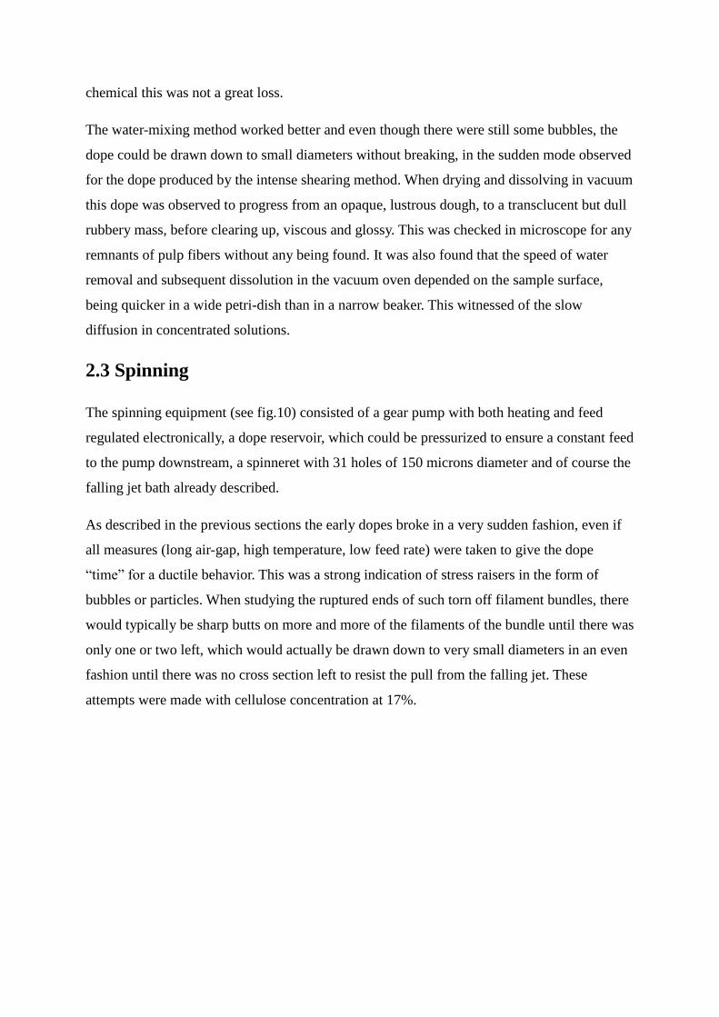
chemical this was not a great loss.

The water-mixing method worked better and even though there were still some bubbles, the

dope could be drawn down to small diameters without breaking, in the sudden mode observed

for the dope produced by the intense shearing method. When drying and dissolving in vacuum

this dope was observed to progress from an opaque, lustrous dough, to a transclucent but dull

rubbery mass, before clearing up, viscous and glossy. This was checked in microscope for any

remnants of pulp fibers without any being found. It was also found that the speed of water

removal and subsequent dissolution in the vacuum oven depended on the sample surface,

being quicker in a wide petri-dish than in a narrow beaker. This witnessed of the slow

diffusion in concentrated solutions.

2.3 Spinning

The spinning equipment (see fig.10) consisted of a gear pump with both heating and feed

regulated electronically, a dope reservoir, which could be pressurized to ensure a constant feed

to the pump downstream, a spinneret with 31 holes of 150 microns diameter and of course the

falling jet bath already described.

As described in the previous sections the early dopes broke in a very sudden fashion, even if

all measures (long air-gap, high temperature, low feed rate) were taken to give the dope

“time” for a ductile behavior. This was a strong indication of stress raisers in the form of

bubbles or particles. When studying the ruptured ends of such torn off filament bundles, there

would typically be sharp butts on more and more of the filaments of the bundle until there was

only one or two left, which would actually be drawn down to very small diameters in an even

fashion until there was no cross section left to resist the pull from the falling jet. These

attempts were made with cellulose concentration at 17%.

In the last attempt made, where the author judges, that there was no longer the problem with

stress raising bubbles, which actually yielded some drawn fibers, the concentration was 15%.

Then fibers successfully passed through the spin bath exit pipe for the first time and were

received by a pair of tweezers to guide it on through the spin-line. Unfortunately it then broke

before a full meter could be retrieved. This was repeated several times. As this “success”

came after shortening the air-gap to some centimeters (compared to decimeters), increasing

flow-speed and lowering the temperature by some 40°C (and still the mode of failure seemed

to be very ductile when studying the ends of the resulting fibers - round), it seems sound to

assume that these were too ductile, providing too little elongational viscosity and elasticity. It

is of course difficult to control whether these very fine fibers broke because of some very

minute bubble or if the radius was decreased beyond a critical value while excessive residence

times allowed relaxations to diminish its strength. However the former kind of explanation

must be considered less probable, as drawing of a viscous solution will equally elongate the

bubble along the stress direction, which reduces its importance as a stress raiser.

Other issues encountered

At the spinneret there was observably a high degree of die swell. If extrusion speed was too

low (≈2 cm/s) the dope would rather tend to cling to the spinneret, forming a drop, which

made fiber formation impossible and demanded wiping of the surface. One way to lessen

Figure 10: schematic 3D-sketch of the spinning equipment.

these tendencies was to smear the surface with silicon oil or detergent, prior to spinning.

When trying to avoid this by increasing the extrusion speed the exiting solution would instead

curl back and forth like a sinus curve. At startup this could cause the end to glue to the

spinneret surface, while the resulting loop descended, which would often interfere with

neighboring filaments.

However most of these problems seemed to straighten out once drawing was applied, which is

to be expected as it decreases residence (relaxation) time and counteracts the curl by the axial

pull.

Filtering is recommended in any fiber spinning operation, as particles are problematic.

Initially there was no filtering and there were several holes blocked, thus not extruding any

solution. Thus filtering was performed with a in-house built device entered into a hydraulic

press, which appeared to avoid these problems. However in the last (most successful) attempt

the solution was not filtered (for technical problems) but still did not appear to clog the

capillaries. When studying the coagulated molding retrieved from inside the spinneret, the

capillaries did in some cases contain dark particles. 5-10 particles, 200 microns wide is not an

awful lot in 80 grams of solution. Thus it seems preferable but not absolutely necessary to

filter in lab scale essays, if only care is taken to keep samples clean.

Feeding the pump with the extremely viscous dopes was also problematic. As they were not

pourable, they had to be scraped out of the beaker into the pressurized container, where they

would not flow to form a flat continuous surface, which even if it did the pressurized air

would probably break through. Thus firstly a plug was needed to stop the air from breaking

through. To simplify the filling procedure cartridges were made so that these could be filled,

mounting the beaker containing the solution upside down, so that its content could run into

the cartridge while drying it in the heated vacuum oven. The idea was also that the rather

bulky cartridge made from Teflon could function as a heat buffer. This seemed quite efficient,

allowed smaller batch sizes and simplified cleaning which is quite frequent and time

consuming when testing many small batches. However the risk of pressure break through

around the cartridge exterior, which caused foaming around the gears of the pump, required

the design of such cartridges to be very precise, why it was discontinued in the last spinning

trials.

The equipment available at the start of the project allowed only pressures supplied by the

local compressors for pneumatic tools (≈6 bar). This proved insufficient for feeding the highly

viscous solutions to the pump, why a new container, capable of holding over 200 bar, was

produced and connected to a nitrogen tube. Generally some 20-30 bar, were applied to

generate a satisfying feed.

The pump regulating functions for flow and particularly temperature were not always valid.

That the blocking of some holes would increase the flow in the remaining was foreseen and

its influence on flow speed could easily be calculated. That the temperature regulator would

be set on and indicating a stable value of 70°C while a drop of water would evaporate

instantly from its surface, like from that of a hot stove, was more distressing. Then it is quite

possible that the solution cooled slightly before reaching the spinneret. It is thus regrettable

that no reliable temperatures could be registered for the trials, even though a probable guess

would be that they were around 80°C for the last trial described above.

2.4 Measurements and testing

To observe the cooling and heating behavior of EmimAc-cellulose solutions a few tests were

performed with standard DC-scan equipment.

Shear viscosity and elasticity of the solutions were investigated by oscillatory and stress

viscometry in a plate-cone viscometer.

Fiber titers were measured by a vibro-scope. The tenacity was then measured in an adjacent

Vibro-dyn equipment, based on those titers, with a gauge length of 20 mm and the elongation

rate 20 mm/min.

The densities of solutions containing 5, 10 and 15 wt% cellulose were measured. The samples

(around 4g each) were placed in containers of aluminum foil (of negligible volume), which

were hung from a frame positioned on a scale (accuracy 0,1 mg). They were then submerged

in paraffin oil, so that the displaced volume of the sample could be deduced as a function of

the paraffin oil density (temperature dependent) and the scale reading. While heating the oil,

temperatures and weights (of displaced paraffin) were registered. The heating device being

rather crude, there were obviously temperature gradients in the paraffin oil (a few °K’s

difference between beaker bottom and surface). When preparing the 10% and 5% samples,

some bubbles were unfortunately mixed into them and they probably disturbed the

measurements some. This was particularly clear when some of them managed to escape in the

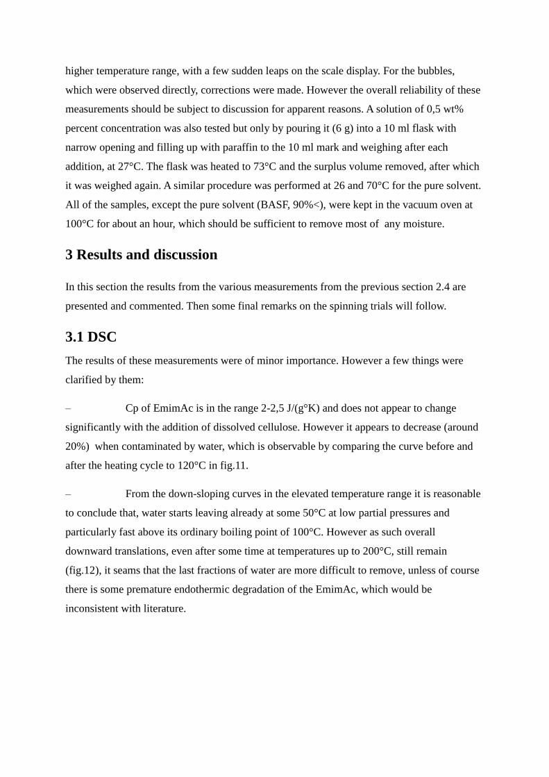
higher temperature range, with a few sudden leaps on the scale display. For the bubbles,

which were observed directly, corrections were made. However the overall reliability of these

measurements should be subject to discussion for apparent reasons. A solution of 0,5 wt%

percent concentration was also tested but only by pouring it (6 g) into a 10 ml flask with

narrow opening and filling up with paraffin to the 10 ml mark and weighing after each

addition, at 27°C. The flask was heated to 73°C and the surplus volume removed, after which

it was weighed again. A similar procedure was performed at 26 and 70°C for the pure solvent.

All of the samples, except the pure solvent (BASF, 90%<), were kept in the vacuum oven at

100°C for about an hour, which should be sufficient to remove most of any moisture.

3 Results and discussion

In this section the results from the various measurements from the previous section 2.4 are

presented and commented. Then some final remarks on the spinning trials will follow.

3.1 DSC

The results of these measurements were of minor importance. However a few things were

clarified by them:

– Cp of EmimAc is in the range 2-2,5 J/(g°K) and does not appear to change

significantly with the addition of dissolved cellulose. However it appears to decrease (around

20%) when contaminated by water, which is observable by comparing the curve before and

after the heating cycle to 120°C in fig.11.

– From the down-sloping curves in the elevated temperature range it is reasonable

to conclude that, water starts leaving already at some 50°C at low partial pressures and

particularly fast above its ordinary boiling point of 100°C. However as such overall

downward translations, even after some time at temperatures up to 200°C, still remain

(fig.12), it seams that the last fractions of water are more difficult to remove, unless of course

there is some premature endothermic degradation of the EmimAc, which would be

inconsistent with literature.

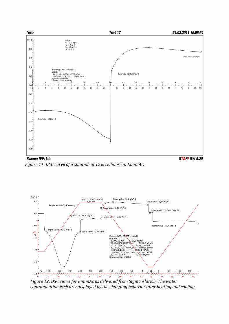
Figure 12: DSC curve for EmimAc as delivered from Sigma Aldrich. The water contamination is clearly displayed by the changing behavior after heating and cooling.

Figure 11: DSC curve of a solution of 17% cellulose in EmimAc.

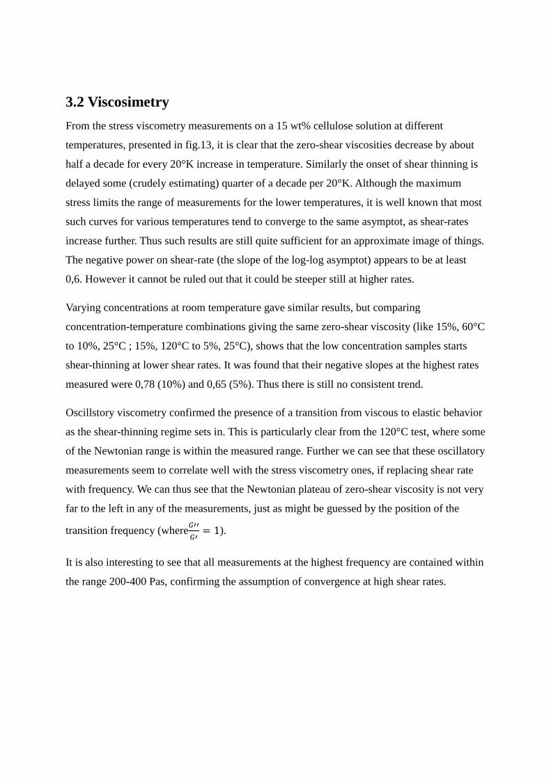
3.2 Viscosimetry

From the stress viscometry measurements on a 15 wt% cellulose solution at different

temperatures, presented in fig.13, it is clear that the zero-shear viscosities decrease by about

half a decade for every 20°K increase in temperature. Similarly the onset of shear thinning is

delayed some (crudely estimating) quarter of a decade per 20°K. Although the maximum

stress limits the range of measurements for the lower temperatures, it is well known that most

such curves for various temperatures tend to converge to the same asymptot, as shear-rates

increase further. Thus such results are still quite sufficient for an approximate image of things.

The negative power on shear-rate (the slope of the log-log asymptot) appears to be at least

0,6. However it cannot be ruled out that it could be steeper still at higher rates.

Varying concentrations at room temperature gave similar results, but comparing

concentration-temperature combinations giving the same zero-shear viscosity (like 15%, 60°C

to 10%, 25°C ; 15%, 120°C to 5%, 25°C), shows that the low concentration samples starts

shear-thinning at lower shear rates. It was found that their negative slopes at the highest rates

measured were 0,78 (10%) and 0,65 (5%). Thus there is still no consistent trend.

Oscillstory viscometry confirmed the presence of a transition from viscous to elastic behavior

as the shear-thinning regime sets in. This is particularly clear from the 120°C test, where some

of the Newtonian range is within the measured range. Further we can see that these oscillatory

measurements seem to correlate well with the stress viscometry ones, if replacing shear rate

with frequency. We can thus see that the Newtonian plateau of zero-shear viscosity is not very

far to the left in any of the measurements, just as might be guessed by the position of the

transition frequency (where

).

It is also interesting to see that all measurements at the highest frequency are contained within

the range 200-400 Pas, confirming the assumption of convergence at high shear rates.

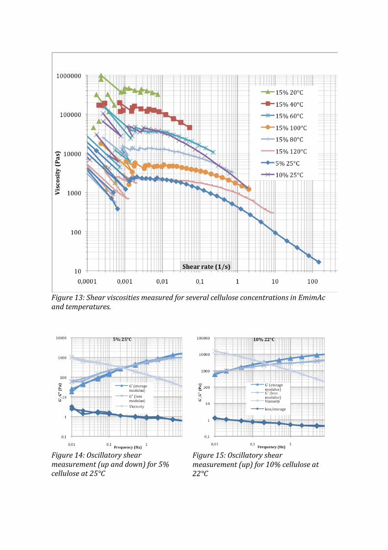
Figure 15: Oscillatory shear measurement (up) for 10% cellulose at 22°C

Figure 14: Oscillatory shear measurement (up and down) for 5% cellulose at 25°C

Figure 13: Shear viscosities measured for several cellulose concentrations in EmimAc and temperatures.

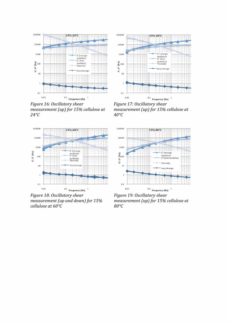
Figure 19: Oscillatory shear measurement (up) for 15% cellulose at 80°C

Figure 18: Oscillatory shear measurement (up and down) for 15% cellulose at 60°C

Figure 17: Oscillatory shear measurement (up) for 15% cellulose at 40°C

Figure 16: Oscillatory shear measurement (up) for 15% cellulose at 24°C

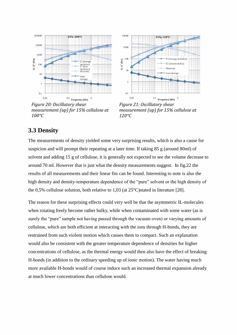
3.3 Density

The measurements of density yielded some very surprising results, which is also a cause for

suspicion and will prompt their repeating at a later time. If taking 85 g (around 80ml) of

solvent and adding 15 g of cellulose, it is generally not expected to see the volume decrease to

around 70 ml. However that is just what the density measurements suggest. In fig.22 the

results of all measurements and their linear fits can be found. Interesting to note is also the

high density and density-temperature dependence of the “pure” solvent or the high density of

the 0,5% cellulose solution, both relative to 1,03 (at 25°C)stated in literature [28].

The reason for these surprising effects could very well be that the asymmetric IL-molecules

when rotating freely become rather bulky, while when contaminated with some water (as is

surely the “pure” sample not having passed through the vacuum oven) or varying amounts of

cellulose, which are both efficient at interacting with the ions through H-bonds, they are

restrained from such violent motion which causes them to compact. Such an explanation

would also be consistent with the greater temperature dependence of densities for higher

concentrations of cellulose, as the thermal energy would then also have the effect of breaking

H-bonds (in addition to the ordinary speeding up of ionic motion). The water having much

more available H-bonds would of course induce such an increased thermal expansion already

at much lower concentrations than cellulose would.

Figure 21: Oscillatory shear measurement (up) for 15% cellulose at 120°C

Figure 20: Oscillatory shear measurement (up) for 15% cellulose at 100°C

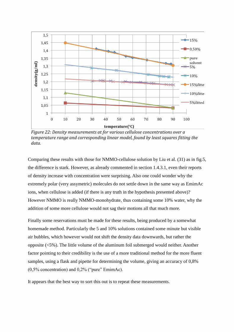
Comparing these results with those for NMMO-cellulose solution by Liu et al. (31) as in fig.5,

the difference is stark. However, as already commented in section 1.4.3.1, even their reports

of density increase with concentration were surprising. Also one could wonder why the

extremely polar (very assymetric) molecules do not settle down in the same way as EmimAc

ions, when cellulose is added (if there is any truth in the hypothesis presented above)?

However NMMO is really NMMO-monohydrate, thus containing some 10% water, why the

addition of some more cellulose would not sag their motions all that much more.

Finally some reservations must be made for these results, being produced by a somewhat

homemade method. Particularly the 5 and 10% solutions contained some minute but visible

air bubbles, which however would not shift the density data downwards, but rather the

opposite (<5%). The little volume of the aluminum foil submerged would neither. Another

factor pointing to their credibility is the use of a more traditional method for the more fluent

samples, using a flask and pipette for determining the volume, giving an accuracy of 0,8%

(0,5% concentration) and 0,2% (“pure” EmimAc).

It appears that the best way to sort this out is to repeat these measurements.

Figure 22: Density measurements at for various cellulose concentrations over a temperature range and corresponding linear model, found by least squares fitting the data.

3.4 Measurements on fibers

Not getting any nice continuous rolls of fiber, although of course a disappointment, did

however yield the possibility to measure an array of differently drawn fibers, not one having

the same draw-ratio as the next with the different properties that resulted, all in one very short

run.

From knowledge of the spinneret hole diameter, density of the dope and cellulose

concentration, the titer of a completely non-drawn fiber can be calculated:

(dTex, in microns), (52)

giving . Obviously all fibers were drawn to some extent (see fig. 7), with draw-

ratios between 1,17 and 6,25. However this is not quite the whole story, as there is typically

die-swell of unknown extent. Either it expresses itself as an actual swell at the die-exit or just

as an initial degree of orientation. Which one of these two alternatives that is valid in this case

Figure 23: comparison of Emimac (at 30 and 90°C) and NMMO-MH (at 30 and 100°C) densities as a function of cellulose concentration.

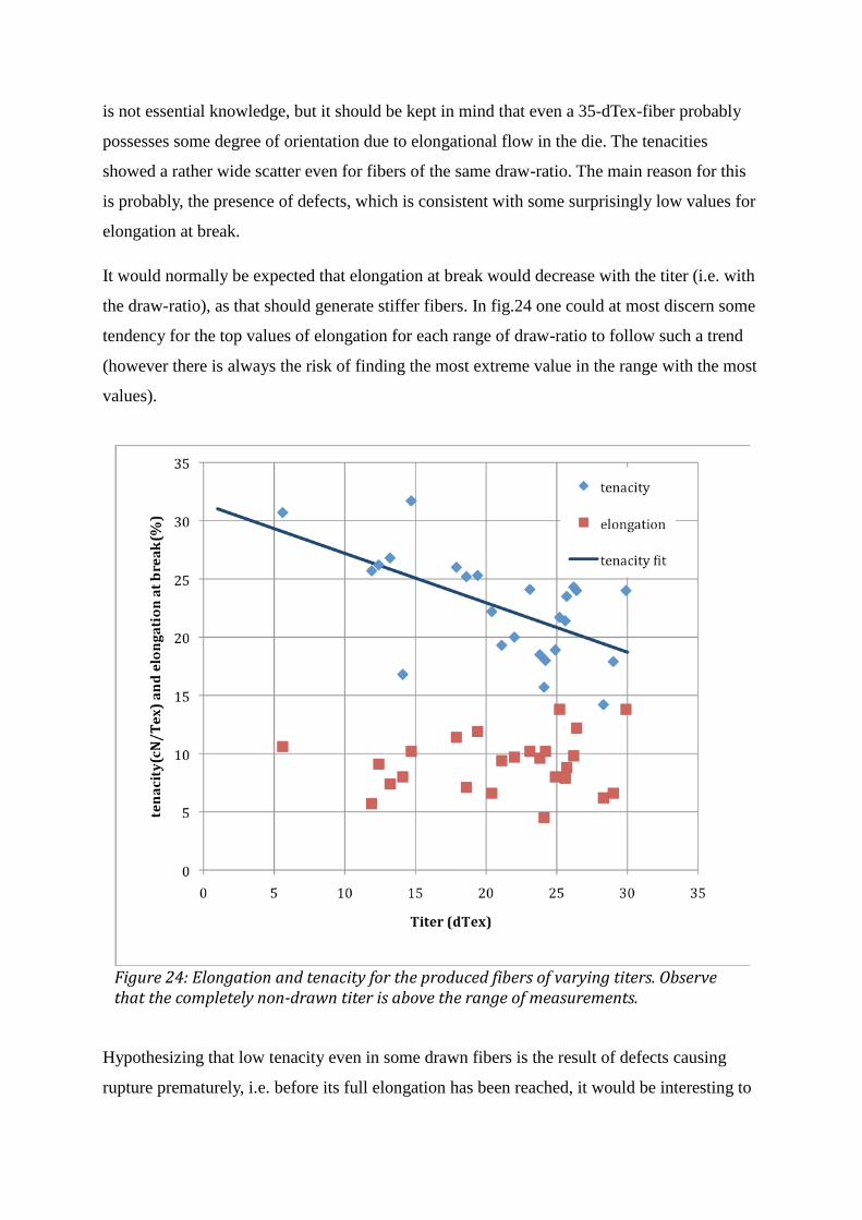
is not essential knowledge, but it should be kept in mind that even a 35-dTex-fiber probably

possesses some degree of orientation due to elongational flow in the die. The tenacities

showed a rather wide scatter even for fibers of the same draw-ratio. The main reason for this

is probably, the presence of defects, which is consistent with some surprisingly low values for

elongation at break.

It would normally be expected that elongation at break would decrease with the titer (i.e. with

the draw-ratio), as that should generate stiffer fibers. In fig.24 one could at most discern some

tendency for the top values of elongation for each range of draw-ratio to follow such a trend

(however there is always the risk of finding the most extreme value in the range with the most

values).

Hypothesizing that low tenacity even in some drawn fibers is the result of defects causing

rupture prematurely, i.e. before its full elongation has been reached, it would be interesting to

Figure 24: Elongation and tenacity for the produced fibers of varying titers. Observe that the completely non-drawn titer is above the range of measurements.

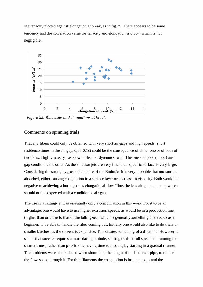
see tenacity plotted against elongation at break, as in fig.25. There appears to be some

tendency and the correlation value for tenacity and elongation is 0,367, which is not

negligible.

Comments on spinning trials

That any fibers could only be obtained with very short air-gaps and high speeds (short

residence times in the air-gap, 0,05-0,1s) could be the consequence of either one or of both of

two facts. High viscosity, i.e. slow molecular dynamics, would be one and poor (moist) air-

gap conditions the other. As the solution jets are very fine, their specific surface is very large.

Considering the strong hygroscopic nature of the EmimAc it is very probable that moisture is

absorbed, either causing coagulation in a surface layer or decrease in viscosity. Both would be

negative to achieving a homogenous elongational flow. Thus the less air-gap the better, which

should not be expected with a conditioned air-gap.

The use of a falling-jet was essentially only a complication in this work. For it to be an

advantage, one would have to use higher extrusion speeds, as would be in a production line

(higher than or close to that of the falling-jet), which is generally something one avoids as a

beginner, to be able to handle the fiber coming out. Initially one would also like to do trials on

smaller batches, as the solvent is expensive. This creates something of a dilemma. However it

seems that success requires a more daring attitude, starting trials at full speed and running for

shorter times, rather than prioritizing having time to meddle, by starting in a gradual manner.

The problems were also reduced when shortening the length of the bath exit-pipe, to reduce

the flow-speed through it. For thin filaments the coagulation is instantaneous and the

Figure 25: Tenacities and elongations at break.

complete removal of EmimAc can be performed in later washing steps.

4 Conclusion

From literature it is clear that cellulose fibers can be made very strong and useful in that they

are not thermoplastics, as most synthetic polymer fibers, if prepared in the proper way.

However those same properties are also what makes it so complicated to produce good fibers.

Some IL’s, of which EmimAc is one, have very special properties in that they do not settle

easily into a low-energy state. This intrinsic instability on the super-molecular scale is

displayed in such phenomena, as their strange variations in density when mixing with other

H-bonders or in their proneness to mix and dissolve them, e.g. cellulose. Therefore they are

one possible solution to the problem of utilizing the properties of cellulose.

To mix spinnable solutions with the IL, EmimAc at high concentrations proved relatively

simple and quick. If bubbles were introduced at any time into the viscous solutions, they

caused problems and could not be efficiently removed. Adding some water to halt dissolution,

allowed stirring more violently while mixing before removing both bubbles and water in a

vacuum oven, where dissolution took place.

The solutions behave a lot like thermoplastic melts in rheology and the available theory for

melt-spinning should be applicable. However while melt-spun fibers solidify gradually, the

stabilizing cooling effect is much lower in air-gap wet-spinning, why solidification is

happening very suddenly when entering the coagulation-bath. Much useful parallels are also

available from the literature on NMMO-spinning.

Fibers could be spun and coagulated in water very quickly. The pull from the flow of the

coagulation bath is problematic if its water pillar is too high, which is unnecessary and

therefore should be avoided. These problems and the tendency for the dope to stick to the

spinneret surface are aided by increased extrusion speed, which makes the falling-jet

apparatus less convenient for lab-scale use. It is a high-speed method for spinning and to use

it at low speed does not return any of its advantages.

For good and consistent results, the climate in the air-gap cannot be overlooked. From the

experiments by other researchers, spinning NMMO-solutions, it appears that it should

preferentially be dry and cool, which it was not in this work.

It is clear, as already shown by Kosan et al. [16], that fibers better than viscose can be

produced with these solvents. The high concentrations and viscosities are central to air-gap

spinning and it was confirmed that the resulting drawing and orientation is the important

factor behind fiber strength.

5 Further development

It appears that the project at hand contained too many steps, each demanding its solution.

Therefore certain things were overlooked in, what appears in hindsight, an overly optimistic

spirit. These are issues that remain.

- The air-gap climate is a central issue that demands controlling. A first step

should be just to confine and measure it. An issue then is how to wipe the spinneret

and fix any unforeseen problems in the confined part. That means redesigning the

equipment so that there are no such needs. To achieve that, the pump would have to

support larger flow rates, so as to allow a wider pipe in the spin-bath while still

maintaining a constant liquid surface level.

In a second step one might start to control temperatures and moisture levels of the

confined air.

- The temperature control at the spinneret would obviously need to be more

accurate, as it is a crucial parameter.

- Performing capillary rheology would increase the understanding of the

elongational flow characteristics, elasticity and die-swell of the solutions.

-

When these remaining issues around consistency and stability of spinning has been solved.

There are many more improvements to take on.

- The first will be optimization of draw-ratios and temperatures.

- Fibrillation can be a problem with highly oriented fibers and it is probably the

case for IL-spun fibers as well.

- Alternative coagulation media is another question, even though water is a very

strong coagulant, it might not be the one providing the best fiber properties.

Before IL-cellulose spinning can be a large-scale industrial process there are of course many,

many more issues, like solvent recovery and the like, which will not be covered here.

6 References

[1] The Ljungberg Textbook Wood Chemistry, Chapter 4 by Helena Lennholm,

Kristina Blomqvist, Printed by the Dept. Of chemical and biological engineering

at Chalmer university of technology in 2008 with the permission of Fibre and

Polymer technology, KTH

[2] The Physics of Polymers 2nd Edition, Gert Strobl, Springer, Berlin, 1997

[3] An introduction to rheology,chapter 5, H.A.Barnes, J.F.Hutton and K.Walters,

1998, Elsevier Science B.V. Amsterdam.

[4] Stephen H. Spiegelberg, Gareth H. McKinley*, Stress relaxation and elastic

decohesion of viscoelastic polymer solutions in extensional flow I, J. of Non-

Newtonian Fluid Mech. 67 (1996)49-76

[5] Imke Diddens, Bridget Murphy, Michael Krisch, and Martin Müller, Anisotropic

Elastic Properties of Cellulose Measured Using Inelastic X-ray Scattering,

Macromolecules 2008, 41, 9755-9759

[6] Antoinette C. O'Sullivan, Cellulose: the structure slowly unravels CELLULOSE

(1997) 4, 173-207

[7] Ullmann's fibers vol.1, p. 335-353, Wiley, 2008, Weinheim, Germany

[8] IL in synthesis vol.1, Peter Wasserscheid, Tom Welton, Wiley, 2008, Weinheim

Germany

[9] Hydrogen Bonds in Imidazolium Ionic Liquids, Kun Dong, Suojiang Zhang,

Daxi Wang, and Xiaoqian Yao, J. Phys. Chem. A 2006, 110, 9775-9782

[10] Ionic Liquids and Their Interaction with Cellulose

Andre´ Pinkert,† Kenneth N. Marsh,*,† Shusheng Pang,† and Mark P. Staiger,

Chem. Rev. 2009, 109, 6712–6728

[11] Kenneth R. Seddon, Annegret Stark, María-José Torres, Influence of chloride,

water, and organic solvents on the physical properties of ionic liquids, Pure

Appl. Chem., Vol. 72, No. 12, pp. 2275–2287, 2000.

[12] Christian Reichardt, Polarity of ionic liquids determined empirically by means

of solvatochromic pyridinium N-phenolate betaine dyes, Green chemistry, DOI:

10.1039/b500106b

[13] Surface Tension Measurements of N-Alkylimidazolium Ionic Liquids

George Law and Philip R. Watson, Langmuir 2001, 17, 6138-6141

[14] Frank Hermanutz, Frank Gaühr, Eric Uerdingen, Frank Meister, Birgit Kosan

New Developments in Dissolving and Processing of Cellulose in Ionic Liquids

Macromol. Symp. 2008, 262, 23–27 DOI: 10.1002/masy.200850203

[15] Richard P. Swatloski, Scott K. Spear, John D. Holbrey, and Robin D. Rogers

Dissolution of Cellose with Ionic Liquids J. AM. CHEM. SOC. 2002, 124,

4974-4975

[16] Birgit Kosan, Christoph Michels, Frank Meister, Dissolution and forming of

cellulose with ionic liquids, Cellulose (2008) 15:59–66

DOI 10.1007/s10570-007-9160-x

[17] Tao Cai, Huihui Zhang, Qinghua Guo, Huili Shao, Xuechao Hu, Structure and

Properties of Cellulose Fibers from Ionic Liquids, Journal of Applied Polymer

Science p. 1047-1053, DOI 10.1002/app

[18] Huihui Zhang, Liwei Guo, Huili Shao, Xuechao Hu,

Nano-Carbon Black Filled Lyocell Fiber as a Precursor for Carbon Fiber,

Journal of Applied Polymer Science, Vol. 99, 65–74 (2006)

[19] Hanneke Boerstohl, Liquid crystalline solutions of cellulose in phosphoric acid

for preparing cellulose yarns, 1998, ISBN: 90-367-0907-5

[20] Kevlar Aramid Fiber, H.H. Yang, 1993, Wiley&sons, Chichester, England

[21] Zhenguo Li a; Panpan Hu a; Junrong Yu a; Zuming Hu a; Zhaofeng Liu a

Preparation and Characterization of Regenerated Cellulose Fibers from a Novel

Solvent System, Journal of Macromolecular Sciencew, Part B: Physics, 47:288–

295, 2008

[22] Regenerated Cellulose Fibres, p.194, Calvin Woodings, Woodhead Publishing

2001, Cambridge, England

[23] Dong Bok Kim,Wha Seop Lee, Seong Mu Jo, Young Moo Lee, Byong Chul

Kim, Physical Properties of Lyocell Fibers Spun from Different

Solution-Dope Phases, Journal of Applied Polymer Science, Vol. 83,

981–989 (2002)

[24] Birgit Kosan, Katrin Schwikal, Frank Meister

Solution states of cellulose in selected direct dissolution agents,

Cellulose (2010) 17:495–506

DOI 10.1007/s10570-010-9402-1

[25] John Eckelt, Tanja Eich, Thomas Ro¨der, Hartmut Ru¨ f, Herbert Sixta,

Bernhard A. Wolf,

Phase diagram of the ternary system NMMO/water/cellulose,

Cellulose (2009) 16:373–379

[26] P.R. Laity, P.M. Glover, J.N. Hay, Composition and phase changes observed

by magnetic resonance imaging during non-solvent induced coagulation of

cellulose,

Polymer 43 (2002) 5827–5837

[27] Olga Biganska and Patrick Navard, Kinetics of Precipitation of Cellulose from

Cellulose-NMMO-Water Solutions,

Biomacromolecules 2005, 6, 1948-1953

[28] Rui-Gang Liu, Yi-Yi Shen, Hui-Li Shao, Cheng-Xun Wu & Xue-Chao Hu,

An analysis of Lyocell fiber formation as a melt–spinning process

Cellulose 8: 13–21, 2001.

[29] Olga Biganska, Patrick Navard,

Morphology of cellulose objects regenerated from cellulose–N-

methylmorpholine N-oxide–water solutions,

Cellulose (2009) 16:179–188

[30] McCorsley, US 4,142,913, 6.Mar 1979

[31] S. A. Mortimer* and A. A. Peguy,

The Influence of Air-Gap Conditions on the Structure Formation of Lyocell

Fibers,

Journal of Applied Polymer Science, Vol. 60, 1747-1756 (1996)

[32] Dong Bok Kim; James Jungho Pak; Seong Mu Jo; Wha Seop Lee,

Dry Jet-Wet Spinning of Cellulose/N-Methylmorpholine N-oxide Hydrate

Solution,

Textile Research Journal; Apr 2005; 75, 4; ProQuest Science Journals, pg. 331

[33] Diffusion of electrolytes in polymers,

Gennadiĭ Efremovich Zaikov, Alekseĭ Leonidovich Iordanskiĭ, Valeriĭ

Sergeevich Markin

1988, Haag

http://books.google.com/books?id=Qaccxq7rj_sC&printsec=frontcover&hl=

sv&source=gbs_ge_summary_r&cad=0#v=onepage&q&f=false

[34] S. A. Mortimer and A. A. Peguy, Methods for Reducing the Tendency of Lyocell

Fibers to Fibrillate,

Journal of Applied Polymer Science, Vol. 60, 305-316 (1996)

[35] H.-P. Fink, P. Weigel, P.J. Purz, J. Ganster, Structure Formation of regenerated

cellulose materials from NMMO-solutions, Prog. Polym. Sci. 26 (2001) 1473-

1524

[36] Tatjana Kreze; Sonja Malej,

Structural characteristics of new and conventional regenerated cellulosic fibers

Textile Research Journal; Aug 2003; 73, 8; ProQuest Science Journals Pg. 675

[37] In Cellulose Solvents: For Analysis, Shaping and Chemical Modification;

Liebert T. et al.

ACS Symposium Series; American Chemical Society: Washington, DC, 2010.

[38] Appendix C5, Incompressible flow, Ronald L. Panton, 2005, New Jersey, Wiley

[39] An introduction to rheology, p.32, H.A.Barnes, J.F.Hutton and K.Walters,

1998, Elsevier Science B.V. Amsterdam.

[40] High-speed fiber spinning, A.Ziabicki, H.Kawai, 1991, Krieger publishing

company, Malabar, Florida

[41] W.M. Jones and I.J. Rees

The stringiness of dilute polymer solutions

Journal of Non-Newtonian Fluid Mechanics, 11 (1982) 257-268

[42] Vishnu T. Marla, Robert L. Shambaugh,* and Dimitrios V. Papavassiliou

Use of an Infrared Camera for Accurate Determination of the Temperature of

Polymer Filaments,

Ind. Eng. Chem. Res. 2007, 46, 336-344

[43] P.90, Incompressible flow, Ronald L. Panton, 2005, New Jersey, Wiley