[AIP LET’S FACE CHAOS THROUGH NONLINEAR DYNAMICS: Proceedings of “Let’s Face Chaos Through...

Energy evolution and exact analysis of the adiabatic invariants in timedependent linear oscillatorMarko Robnik and Valery Romanovski Citation: AIP Conf. Proc. 1076, 185 (2008); doi: 10.1063/1.3046254 View online: http://dx.doi.org/10.1063/1.3046254 View Table of Contents: http://proceedings.aip.org/dbt/dbt.jsp?KEY=APCPCS&Volume=1076&Issue=1 Published by the American Institute of Physics. Related ArticlesOn the completely integrable case of the Rössler system J. Math. Phys. 53, 052701 (2012) Generalized complexity measures and chaotic maps Chaos 22, 023118 (2012) On finite-size Lyapunov exponents in multiscale systems Chaos 22, 023115 (2012) Exact folded-band chaotic oscillator Chaos 22, 023113 (2012) Components in time-varying graphs Chaos 22, 023101 (2012) Additional information on AIP Conf. Proc.Journal Homepage: http://proceedings.aip.org/ Journal Information: http://proceedings.aip.org/about/about_the_proceedings Top downloads: http://proceedings.aip.org/dbt/most_downloaded.jsp?KEY=APCPCS Information for Authors: http://proceedings.aip.org/authors/information_for_authors

Downloaded 07 May 2012 to 132.236.27.111. Redistribution subject to AIP license or copyright; see http://proceedings.aip.org/about/rights_permissions

http://proceedings.aip.org/?ver=pdfcov

http://aipadvances.aip.org?ver=pdfcov

http://scitation.aip.org/vsearch/servlet/VerityServlet?KEY=ALL&uSeDeFaUlTkEy=TrUe&possible1=Marko Robnik&possible1zone=author&maxdisp=25&smode=strresults&aqs=true&ver=pdfcov

http://scitation.aip.org/vsearch/servlet/VerityServlet?KEY=ALL&uSeDeFaUlTkEy=TrUe&possible1=Valery Romanovski&possible1zone=author&maxdisp=25&smode=strresults&aqs=true&ver=pdfcov


http://link.aip.org/link/doi/10.1063/1.3046254?ver=pdfcov

http://proceedings.aip.org/dbt/dbt.jsp?KEY=APCPCS&Volume=1076&Issue=1&ver=pdfcov

http://www.aip.org/?ver=pdfcov







http://proceedings.aip.org/about/about_the_proceedings?ver=pdfcov

http://proceedings.aip.org/dbt/most_downloaded.jsp?KEY=APCPCS&ver=pdfcov

http://proceedings.aip.org/authors/information_for_authors?ver=pdfcov

Energy evolution and exact analysis of the adiabatic invariants in time-dependent linear

oscillator Marko Robnik and Valery Romanovski

CAMTP - Center for AppliedMathematics andTheoretical Physics, University ofMaribor, Krekova 2, SI-2000 Maribor, Slovenia

E-mail: [email protected] and [email protected]

Abstract. The theory of adiabatic invariants has a long history, and very important implications and applications in many different branches of physics, classically and quantally, but is rarely founded on rigorous results. Here we treat the general time-dependent one-dimensional linear (harmonic) oscillator, whose Newton equation q+ aP'{t)q = 0 cannot be solved in general. We follow the time-evolution of an initial ensemble of phase points with sharply defined energy EQ at time / = 0 (microcanonical ensemble) and calculate rigorously the distribution of energy £1 after time^ = T, which is fully (all mjaments, including the variance p?) determined by the first moment £1 . For example, jx^ = EQ[{E-I/EO)^ — {a>{T)/a>{0))^]/2, and all higher even moments are powers of/J^, whilst the odd ones vanish identically. This distribution function does not depend on any further details of the function a>{t) and is in this sense universal, it is a normalized distribution function given by P(x) = ;i:^^(2/j^ —x^)^^, where x = £'i —E-i.E-i and/j^ can be calculated exactly in some cases. In ideal adiabaticity £1 = a>{T)Eo/a>{0), and the variance fi^ is zero, whilst for finite T we calculate Ei, and /J^ for the general case using exact WKB-theory to all orders. We prove that if (o{t) is of class ' ™ (all derivatives up to and including the order m are continuous) ji oc f-ii^+i)^ whilst for class '^°° it is known to be exponential /j oc exp(—aT). Due to the positivity of/J^ we also see that the adiabatic invariant I =Ei/a>i at the average energy Ei never decreases.

Keywords: nonlinear dynamics, nonautonomous Hamiltonian systems, adiabatic invariants, energy evolution, statistical mechanics, microcanonical ensemble PACS: 05.45.-a,45.20.-d, 45.30.+S, 47.52.+J

INTRODUCTION

This review paper covers the topics of our recent research on the adiabatic invariants and the energy evolution as well as its statistical properties in the time-dependent hnear oscillator, with the oscillation frequency being an arbitrary function of time, and also allowing for arbitrary external forcing. It thus comprises a series of four papers so far [1, 2, 3, 4], although not much wiU be presented about external forcing analyzed in [4].

In time-independent (autonomous) Hamiltonian systems the total energy of the system is conserved by construction, i.e. due to the Hamilton equations of motion, and the LiouviUe theorem applies, because the phase flow velocity vector field has vanishing divergence. In time-dependent (nonautonomous) Hamilton systems the total energy is not conserved, whilst the LiouviUe theorem still applies, the phase space volume is preserved under the phase flow. If (some parameter of) the Hamilton function varies in time, the energy of the system generally also changes. But, if the changing of the

CP1076, Let's Face Chaos Through Nonlinear Dynamics: 7 International Summer School and Conference edited M. Robnik and V. Romanovski

© 2008 American Institute of Physics 978-0-7354-0607-0/08/$23.00

185


mailto:[email protected]

mailto:[email protected]

parameter is very slow, on the typical time scale T, there might be a quantity /, a function of the said parameter, of the energy E and of other dynamical quantities, which is approximately conserved. It might be even exactly conserved if T ^ ^, i.e. if the variation is infinitely slow, to which case we refer as the ideal adiabatic variation. Such a conserved quantity is called adiabatic invariant, and it plays an important role in the dynamical analysis of a long-time evolution of nonautonomous Hamilton systems.

The theory of adiabatic invariants is aimed at finding the adiabatic invariants / and analyzing the error of its preservation at finite T. Namely, the statement of exactness in preservation of/ is asymptotic in the sense that the conservation is exact in the hmit T ^ ^, whilst for finite T we see the deviation AI = II—IQ of final value of /i from its initial value /Q and would like to calculate A/. Thus for finite T the final values of / i , like the final values of the energy Ei, will have some distribution with nonvanishing variance. Indeed, for one-dimensional harmonic oscillator it is known since Lorentz and Einstein [5] that the adiabatic invariant for T = oo is / = E/co, which is the ratio of the total energy E = E{t) and the frequency of the oscillator co{t), both being a function of time. Of course, Inl is exactly the area in the phase plane {q,p) enclosed by the energy contour of constant E. A general introductory account of the theory of adiabatic invariants can be found in [6] and references therein, especially [7], [8].

However, in the literature this / and A/ are not even precisely defined. It turns out that / must be generally considered as a function of the initial conditions, and then it turns out that it is conserved for some initial conditions but not for some others. As a consequence of that there is a considerable confusion about its meaning. Let us just mention the case of periodic parametric resonance (see the relevant section below), with otherwise arbitrarily slowly changing co{t), in one-dimensional harmonic oscillator, where the total energy of the system can grow indefinitely for certain (almost all) initial conditions, and since co{t) is bounded, / = E{t)/co{t) simply cannot be conserved for the said initial conditions for all times, but only for sufficiently small times. In this paper we consider / as a function of the initial conditions, and give a precise meaning to these and similar statements.

Therefore to be on rigorous side we must carefully define what we mean by / and A/. This can be done by considering an ensemble of initial conditions at time t = 0 just before the adiabatic process starts. Of course, there is a vast freedom in choosing such ensembles. Let us consider the one degree of freedom systems, which is the topic of this paper If the initial conditions are on a closed contour ^ in the phase space at time / = 0, then at the end of the adiabatic process at time t = T they are also on a closed contour ^ which in general is different from ^ , but due to the Liouville theorem the area inside the contour is constant for all T. If ^ is a contour of constant energy at time / = 0, then ^ generally is not a contour of constant energy of the Hamiltonian at time T. The final energies of the system, depending on the initial conditions, are spread and thus distributed between some minimal and maximal energy, Emm and Emax, respectively. In the said case of periodic co{t) and parametric resonance in a harmonic oscillator the contour ^ is squeezed in one direction and expanded in the other one (the transformation is a hnear map), and this contraction and expansion is exponential in time. Therefore, I = E{T)/co{T) can not be conserved.

Thus we must always study / as a function of initial conditions, by looking at the ensembles of initial conditions. There is a considerable multitude of possibilities in

186


choosing such ensembles, but usually we do not know very much about the system except e.g. just the energy.

Therefore in an integrable conservative Hamiltonian system the most natural and the most important case (choice) is taking as the initial ensemble all phase points uniformly distributed on the initial TV-torus, i.e. uniform w.rt. the angle variables. We call it uniform canonical ensemble of initial conditions. Such an ensemble has a sharply defined initial energy EQ. Then we let the system evolve in time, not necessarily slowly, and calculate the probability distributionP(iii) of the final energy Ei, or of other dynamical quantities. Typically E\ is distributed on an interval {Emin,Emax), and P{E\) is universal there, as it does not depend on any further properties of «(/) except for Ei. More general ensembles of initial energies W{EQ) can be described in terms of the uniform canonical ensembles, as explained in the last section.

To describe P{Ei) is in general a difficult problem, but in this work we confine ourselves to the one-dimensional general time-dependent harmonic oscillator, so TV = 1. We do not consider the external forcing any further, but the details can be found in [4]. The system is described by the Newton equation

q + (0^{t)q = () (1)

and we work out rigorously P{E\). Given the general dependence of the oscillator's frequency (i){t) on time t the calculation of qlt) is already a very difficult, in fact unsolvable, problem.' Nevertheless, we can calculate P{E\) and it turns out to be surprisingly simple and universal (independent of «(/)), namely we find the so-called arc sine distribution

where x = Ei—Ei. In performing our analysis, we shall answer the questions as to when is

I = E{T)/co{T) conserved, and if it is not conserved, what is the spread or variance jj.^ of the energy, and the higher moments etc. Then (the not sharply defined) A/ in the literature is proportional to ji, namely AI ^ ji/co. After performing the exact analysis, we provide a powerful technique based on the WKB method [9] to calculate jj.^, and show that it gives exact leading asymptotic terms when T ^ ^, and moreover, generally we can do the expansion to all orders, exactly. We treat several exactly solvable cases, and compare them with the WKB results, and finally prove the theorem as for how ji^ behaves when «(/) is of class ' ™, which means having m continuous derivatives.

We give a brief historical review of contributions to this field. After Einstein [5], Kulsrud [10] was the first to show, using a WKB-type method, that for a finite T, I

In the sense of mathematical physics (1) is exactly equivalent to the one-dimensional stationary Schrodinger equation: the coordinate q appears instead of the probability amplitude ^/, time / appears instead of the coordinate x and (»^(/) plays the role of # — V{x) = energy - potential. If S is greater than any local maximum oiV{x) then the scattering problem is equivalent to our ID harmonic oscillator problem.

187


is preserved to all orders, for harmonic oscillator, if all derivatives of (o vanish at the beginning and at the end of the time interval, whilst in case of a discontinuity in one of the derivatives he estimated A/ but did not give our explicit general expressions (70) and (71). Hertweck and Schltiter [ 11 ] did the same thing independently for a charged particle in slowly varying magnetic field for infinite time domain. Kruskal, as reported in [12], and Lenard [13] studied more general systems, whilst Gardner [12] used the classical Hamiltonian perturbation theory. Courant and Snyder [14] have studied the stability of synchrotron and analyzed / employing the transition matrix. The interest then shifted to the infinite time domain. Littlewood [15] showed for the harmonic oscillator that if co{t) is an analytic function, / is preserved to all orders of the adiabatic parameter e = 1/T. Kruskal [16] developed the asymptotic theory of Hamiltonian and other systems with all solutions nearly periodic. Lewis [17], using the Kruskal's method, discovered a connection between / of the 1 -dim harmonic oscillator and another nonlinear differential equation. Later on Symon [18] used the Lewis'es results to calculate the (canonical) ensemble average of the / and its variance, which is the analogue of our Ei and ji^. Finally, Knorr and Pfirsch [19] proved A/ oc Qxp{—const/e). Meyer [20], [21] relaxed some conditions and calculated the constant const. Exponential preservation of/ for an analytic co on (—°°, +°°) with constant limits at / ^ ±°°, is thus well established [7].

THE TRANSITION MAP AND GENERAL EXACT CONSIDERATIONS

We begin by defining the system by giving its Hamilton function/f = H{q,p,t), whose numerical value E{t) at time t is precisely the total energy of the system at time t, and for the general time-dependent one-dimensional harmonic oscillator this is

where q,p,M,co are the coordinate, the momentum, the mass and the frequency of the linear oscillator, respectively. The dynamics is linear in q,p, as described by (1), but nonlinear as a function of co{t) and therefore is subject to the nonlinear dynamical analysis. By using the index 0 and 1 we denote the initial (t = to) and final {t = ti) value of the variables, and by T = ti—to we denote the length of the time interval of changing the parameters of the system.

We consider the phase flow map (we shall call it transition map)

Because equations of motion are linear in q and p, and since the system is Hamiltonian, O is a linear area preserving map, that is.

188


with det(O) = ad — be = 1. Let EQ = H{qo,po,t = to) be the initial energy and Ei = H{q\,p\,t = ti) be the final energy, that is.

£ i = -1 f{cqo + dpo

-Ma)j{aqo + bpo) 2\ M

Introducing the new coordinates, namely the action/ = E/co and the angle (j).

(6)

from (6) we obtain

where

<?o= J-—^cos(j), po= \/2MEosm(j)

El = Eo{acos^ (j) + P sir^ (j) + Ysin2(j)),

(7)

(8)

a = Afico^ _«2^^ /3 = J 2 ^ « 2 M V , 7= ''"'

ft), M(0o cot

-abM-^. (Oo

(9)

Given the uniform probability distribution of initial angles (/) equal to l/{2n), which defines our initial uniform canonical ensemble (microcanonical ensemble) at time t = to, we can now calculate the averages. Thus

Ei = ^JEid<\> = ^{a + fi]

That yields i?i —Ei =£'o(5cos2(/) +7sin2(/)) and

(10)

E'. M2 = ( i ? i - i ? i ) 2 = ^ ( 5 2 + y2) (11)

where we have denoted 5 = (a — /3 )/2. It follows from (9), (10) that we can write (11) also in the form

M2=(i?i-i?i)2 = f (12)

As we shall see, in an ideal adiabatic process ji = Q, and therefore Ei= Ei = COIEQ/COQ, and consequently P{Ei) is a delta function.

P{Ei) = 5{Ei-a)iEo/(Oo) (13)

Now we calculate higher moments of P(i?i). Let us show that in general for arbitrary positive integer m

( £ l - £ l ) 2 ' « - l = 0 (14)

and

189


("2/72— IV I / \™ (i?l-i?l)2" = ^ ^ ^ ^ ^ ^ ( ( i ? l - i ? l ) 2 ) . (15)

It is easy to check the correctness of (14), so we prove only (15). Indeed,

{El -Ei)^ = £'^"'(7sin2(/) + 5cos2(/))2»' = (16)

2" ^2m ^ o " S r. )(r^"*5*sin2™-*2(/)cos*2(/))

Note that for odd A: = 2/ - 1

sin2"'-*2(/)cos*2(/) = 0. (17)

Therefore we can rewrite (16) in the form

2m {Ei-Ei)^"'=E^^[ (72'«-2/52'sin2'«-2/20cos2'2(/)). (18)

Using formula 2.512 of [22] we obtain

f r ^^"-•'1,0.^1,,, ^ ' ^ ' - " " g " ; ^ ' - " " (19, 2n Jo 2™/w!

The substitution of this value into (18) yields

" /toV 2'«/H!(2/)!!(2/H-2/)!!y' ^ ^

Er^^^^^^^li^'y-^'S- (22) 2™/wl

(23)

that is, the formula (15) holds. Thus 2/w-th moment of P{Ei) is equal to {2m — \)\\ji^"'/m\, and therefore, indeed, all moments of P(i?i) are uniquely determined by the first moment Ei.

Expression (12) is positive definite by definition and this leads to the first interesting ci)nclusion: In full generality (no restrictions on the function (i){t)\) we have always E\ > Eo(i)\J(i)o and therefore the final value of the adiabatic invariant (for the average energy!) I\ = Ei/coi is always greater or equal to the initial value /o = Eo/coo. In other words, the value of the adiabatic invariant at the mean value of the energy never decreases, which is a kind of irreversibility statement. Moreover, it is conserved only for infinitely slow processes T = ^, which is an ideal adiabatic process, for which 11 = 0. For periodic processes coi = COOWQ see that always Ei >Eo, so the mean energy

190


never decreases. See subsequent sections. The other extreme opposite to T = oo is the instantaneous (T = 0) jump where coo switches to coi discontinuously, whilst q and p remain continuous, and this results ma = d = I and b = c = 0, and then we find

^ ( ^ + 11 U^-^ ^ _ 1 7

ft). (24)

'0

Below we shall treat the special case with coj = 2C0Q, and thus will find ji^/EQ = 1/8 = 0.125.

Our general study now focuses on the calculation of the transition map (5), namely its matrix elements a,b,c,d. Starting from the Hamilton function (3) and its Newton equation (1) we consider two linearly independent solutions ^\{t) and i//2(0 ^^'^ introduce the matrix

(25)

Consider a solution q{t) of (1) such that

q{to) = qo, 4{to) = Po/M. (26)

Because Xjfi and yfj are hnearly independent, we can look for q{t) in the form

q{t)=Axi/i{t)+Bxi/2{t). (27)

Then^ and B are determined by

i)^r'M[2). (28) Leti^i = q{ti), pi =Mq{ti). Then from (26)-(28) we see that

^ ; ) ^ ^ ( , ) ^ - ( . o ) ( ^ : ) . (29)

We recognize the matrix on the right-hand side of (29) as the transition map O, that is,

'j'=f! t)=nh)^-\to). (30) c d

THE FINAL ENERGY DISTRIBUTION FUNCTION

Now we derive the distribution function (2) using the characteristic function f{y) of P{x), namely

f{y) = j°^j'y''P{x)dx. (31)

We see immediately that the «-th derivative atj^ = 0 is equal to

191


/ W ( 0 ) = / " {ix)"P{x)dx = i"a„, (32)

where C7„ is the «-th moment of P(x) (in particular 02 = l~i^), ie .

a„= [ x"P{x)dx. (33)

A'^) (0) Using the Taylor expansion for f{y) = Sr=o „! >*" and the expressions (15) we see at once

and using the formula (2/w— 1)!! = (2/w)!/(2™/w!), we obtain,

/W=S - ^ 77^' (35)

which can be summed and is equal to the Bessel function [22]

fiy)=MnyV2). (36) Knowing the characteristic function (31,36) we now only have to invert the Fourier transform, namely

P{x) = ^ fj-'V{y)dy = ^ fj-^MV2^y)dy, (37)

which is precisely equal to (2) for |x| < ^ v ^ and is zero otherwise. (See reference [22].) Indeed, the distribution (2) is normahzed to unity as it must be. It is essentially the so-called /3(l/2,1/2) distribution or also termed arc sine density [23], after shifting the origin of x to 1/2 and rescahng of x. It is obvious that the distribution function does not depend on any details of co{t) and is in this sense universal for ID time-dependent harmonic oscillator in case of uniform canonical ensemble of initial conditions, i.e. uniform w.rt. the canonical angle.

The rigorous method of calculating Ei and ji^ was explained above, and in the general case when (1) cannot be solved exactly, the WKB method [9] can be ajplied to all orders, first to get the transition map (its matrix elements a,b,c,d), and theniii and ji^, as shown in the next sections.

Let us now present the direct algebraic derivation of the energy distribution function (2). By definition we have (see the expression before equation (11))

d(j)

dEi (38)

<l>=<l>j(Ei)

where we have to sum up contributions from all four branches of the function (/)(i?i) Let us denote x = Ei — Ei, so that we have

192


x = £'o(5cos(2(/)) + 7sin(2(/))) = iiV2sm{2^ + \i/), (39)

where 5 = (a — /3)/2, and a, /3 and 7 are expressed in terms of a,b,c,d as shown -"0 2 in equation (9), the variance is as in equation (11), namely ji^ = -j-{S^ + 'f'), and

tan I// = 5/7, so that (/) = ^arcs in^^ — ^ . Therefore | -^ | = —1=—j for all four

solutions /• = 1,2,3,4 and from (38) we get (2) at once. The first derivation demonstrates the power of the approach employing the charac

teristic function f(y) of P(x), giving us new insights, whereas the second one leads elegantly to the final result, eliminating many parameters by a rather elementary substitution. In fact, this second method is geometrically obvious by the following argument: In phase space, the initial distribution lies on an ellipse. The final distribution lies on a different ellipse with the same area, with the points equidistributed in the canonical angle variable. This final ellipse intersects the energy contours of the Hamiltonian, and thus after squeezing the final Hamiltonian so that its energy contours are circles, the desired probability distribution is simply the distribution of radii of those circles through which the final ellipse passes. The graph of the distribution function (2) is shown in figure 3. We remark that if we include arbitrary time-dependent external forcing, the structure of P{E\) becomes quite complex. For details see [4].

In nonlinear systems the entire theory expounded originally in [1, 2, 3] and reviewed in this paper, must be reformulated and as such it is an important open problem [24]. For the case of a separatrix crossing some interesting numerical results have been obtained in [25], namely P{Ei) there has a substantial structure and is by far not so simple as (2).

SOME EXACTLY SOLVABLE CASES

The theory of adiabatic invariants is rarely founded on rigorous results, therefore the study of exactly solvable cases is of fundamental importance, namely we can use them to test various analytic approximations and also the accuracy of numerical calculations. Because the ideal adiabatic processes are infinitely slow and refer to the limit T ^ 00 we must deal necessarily with the asymptotic behaviour of dynamical systems, which is difficult to approximate, because all simple minded perturbational and other approximation techniques fail (break down) after some finite time, and so typically give wrong predictions for the asymptotic behaviour in the limit T ^ ^. The same difficulty occurs in numerical calculations. We shall see that the WKB methods [9] can be successfully applied. In this section we deal with three different models for the function (a^{t).

The linear model: class 'lo^

We assume that function a>^{t) is a piecewise linear function of the form

193


(0^ if t<0

(oHt)={ a)^ + i^:^t ifO<t<T- (40) (oj if t>T

Thus co{t) has discontinuous first derivative at / = 0 and t = T, and belongs to the class '^''. Introducing the notation a= COQ, b = coj — COQ WQ obtain that on the interval (0, T) the equation (1) has the form

q+{a+Y)q = 0. (41)

Two hnear independent solutions of (41) are given by the Airy functions:

'/^iW=^'\p7J^j (42)

and

y^m^B,(^). (43)

The elements a,b,c,d of the matrix Oj- are defined by the equation (29) and (30). The exact analytic expression for

^^ = {E,-E,r = ^{5^ + Y') (44)

is very complex, and we do not show it here. However, for WQ = 1, o) = 2, iio = 1, using the asymptotic expansion 10.4.60,62,64,66 of [26] (pp.448-449), we obtain the following approximation

(El-El?-^{^ | ^ 9 - 4 V 2 c o s ( ^ ^ ^ ) ' j , (45)

where we introduce the adiabatic parameter e,

e = . (46)

We see in figure 1 that the exact expression (44) and its leading asymptotic approximation (45) practically coincide, which demonstrates the power of the asymptotic expansion of the relevant expressions containing the Airy functions. Observe that the decay of jj.^ to zero as e 0 is oscillatory but quadratic on the average, namely as >> = ^ e ^ , which means that ji goes to zero linearly with the adiabatic parameter e. This is always the case when co{t) is of class '^''. As we will see, in general, if co{t) is of class ' ™, then II goes to zero oscillatory but in the mean as a power e™+^ This theorem will be proven in the next section using the exact formulation of the WKB method, applied to

194


FIGURE 1. /J^ = (£1 —Ei)"^ forO< e < 0.05; the lines ofthe exact expression (44) and the asymptotics (45) practically coincide; the non-oscillating thin line is the parabola>' = ffoe^-

FIGURE 2. At = {E\ -Eif iorQ<e< 1.2; the lines ofthe exact expression (44) (full) and ofthe asymptotics (45) (dashed) practically coincide for e < 0.3; the non-oscillating thin line is the parabola y = ^fgE^- One can show that p? goes to 1/8 = 0.125 when e ^ 00, which means T ^ 0, which means the instantaneous jump of iMo = 1 to Oi = v'2.

the relevant (but arbitrarily high) order We shall see that the leading WKB term precisely reproduces the exact leading term in (45). In figure 2 we show the same thing as in figure 1 but on the larger scale of e.

In figure 3 we show the emerging distribution function as an illustration.

195


275

250

225

200

175

150

125

io_a 1 . 4 1 2 1 . 4 1 3 1 . 4 1 4 1 . 4 1 5 1 . 4 1 6 1 . 4 1 7

FIGURE 3. The distribution function P(£'i) for the linear model foriio = l,<»o = 1,<» = 2,e = 0.01.

The harmonic model: class ^ ^

Now we consider the case when co{t)is of class "^^ namely we use the specific model

co\t) {b-a)cos{f)0<t<T if t<0

)<t<T if t>T

where a = WQ , 2b — a = (0^. Then the equation (1) has the form

q+(i-{b-a) cos (^yj jq = 0

and the fundamental solutions are represented by the Mathieu functions:

f4bT^ 2{b-a]T^ nt

IT

and

W2{t) 4bT^ 2{b-a)T^ nt

(47)

(48)

(49)

(50)

In this model the first derivative of «(/) vanishes at / = 0 and t =T and is continuous there, whilst the second derivative is discontinuous, therefore «(/) belongs to the class

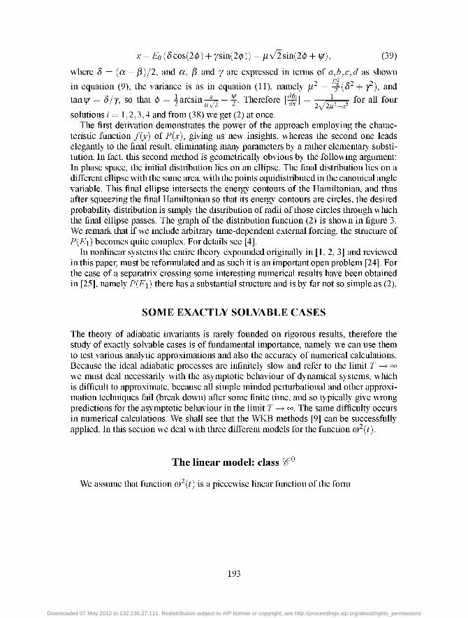
Here we find that indeed ji^ goes to zero oscillating but in the mean as e'*, as shown in figure 4. The exact analytic asymptotic behaviour of the Mathieu functions needed for our calculations is not known, unlike for the Airy functions, but we compare the exact (numerical result) with the WKB approximation expounded in the next section, see the final general formula (104).

196


0.00008 -

0.00002 -

FIGURE 4. We show, for the harmonic model of subsection 3.2, ji^ = {Ei — £1)2 for 0 < e < 0.1. The exact result is represented by the full line, whilst the dashed curve is the curve 0.0566" ( 4 1 + 9 c o s ( 2 ^ ) ) , obtained by the WKB method, equation (104).

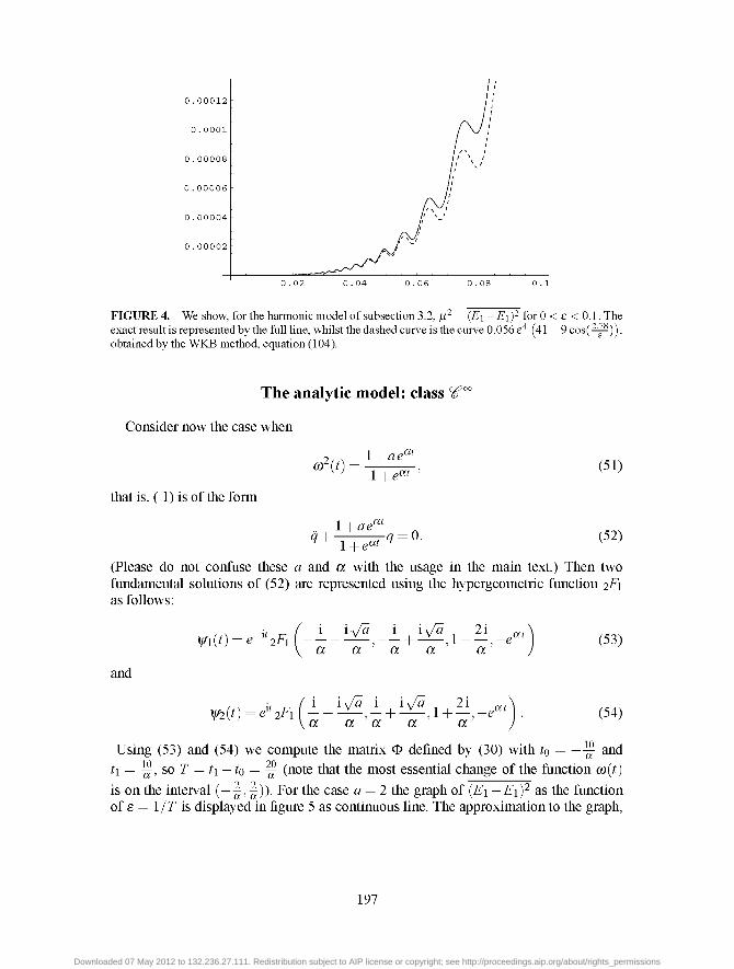
The analytic model: class ^

Consider now the case when

«'(0 = 7—^, (51)

that is, ( 1) is of the form

^ + T ^ ^ ? = 0- (52)

(Please do not confuse these a and a with the usage in the main text.) Then two fundamental solutions of (52) are represented using the hypergeometnc function 2F\ as follows:

if / i iJa i iJa 2i „ , \ Wi{t) = e-''2FA ^ , + ^ ^ , l - - , - e « M (53)

\ a a a a a J

and

•f / i iJa i iJa 2i „A W2{t) = e''2FA ^ , - + ^ ^ , l + - , - e « M . (54)

\a a a a a J Using (53) and (54) we compute the matrix O defined by (30) with k = —^ and

t\ = ^, so T = t\ — to = ^ (note that the most essential change of the function «(/)

is on the interval (—^, ^)). For the case a = 2 the graph of {E\ —E\)^ as the function of e = 1/r is displayed in figure 5 as continuous line. The approximation to the graph,

197


0 . 0 0 0 0 1 2

0 . 0 0 0 0 1

8

6

4

2

• 1 0 - ^

• 1 0 - ^

• 1 0 - ^

• 1 0 - ^

0 . 0 3 5 0 . 0 4 0 . 0 4 5 0 . 0 5

FIGURES. The variance/J^ = {Ei —EiY ofthe energy for the analytic model (51), for 0.03 < e <0.05. The dashed curve is approximation>• = 4.174e^'''*^'''''.

y = 4.174e " 634/e computed using the least square method, is displayed in the figure as dashed line. We clearly see that the behaviour of ^^ is exponential.

A N APPLICATION OF THE W K B THEORY TO COMPUTE THE VARIANCE jU

General and exact considerations

In this section we proceed with the calculation of the transition map O in the general case, and because (1) is generally not solvable, we have ultimately to resort to some approximations. Since the adiabatic limit e ^ 0 is the asymptotic regime that we would like to understand, the application ofthe rigorous WKB theory (up to all orders) is most convenient, and usually it turns out that the leading asymptotic terms are well described by just the leading WKB terms if e is sufficiently small. In using the WKB method we refer to our work [9], where we have derived the explicit analytic expressions for all WKB orders in closed form, except for the exact rational coefficients, which can be easily obtained from a recurrence formula . The WKB method, when worked out to all orders, and when the series is convergent, has the potential to be exact and rigorous provided that the underlying series converges.

^ There is substantial literature on WKB method, which due to limited space cannot be reviewed here. But we should mention the classic works by N. Froman and P.O. Froman, who have found a number of interesting relationships, e.g. a relation between the even and odd order terms [27], although we do not use it here, so that our exposition is selfcontained.

198


We introduce re-scaled and dimensionless time X

X = et, e = l/T, (55)

so that (1) is transformed to the equation

e^q"{X) + CO^{X)q{X)=0. (56)

By prime we denote the differentiation w.rt. X. Let q+{X) and q-{X) be two linearly independent solutions of (56). Then the matrix (25) takes the form

vp, - / ?+(^) ?-(^) ^ r57^ ^ ^ \ eMq'+{X) eMq'_{X) ) ^^''

and taking into account that XQ = eto, Xi = et\, we obtain for the matrix (5) the expression

^=[l * ) = ^ , ( A i ) ¥ ^ i ( A o ) . (58)

We now use the WKB method in order to obtain the coefficients a,b,c,d of ihs matrix O. To do so, we look for solution of (56) in the form

? (A)=wexp | - c7 (A) l (59)

where C7(A) is a complex function that satisfies the differential equation

{G'{X)f + eG"{X) = -oi^{X) (60)

and w is some constant with dimension of length. The WKB expansion for the phase is

cT(A)=£e*cTi(A). (61)

Substituting (61) into (60) and comparing like powers of e gives the recursion relation

cT2 = _o)2(A), a'„ = -^"j^o',o'„_, + o'l,). (62) ^ " o k=l

Here we apply our WKB notation and formahsm from our work [9] and we can choose O'Q ^ ( A ) = \(i){X) or C7Q _ ( A ) = —\(i){X). That results in two linearly independent solutions of (56) given by tfie WKB expansions with the coefficients

c7o,±(A) = ± i / (o{x)dx, c7i,±(A) = - - l o g ; ' (63) JXo I ft)(Aoj

C72,± = ± ^ / — —f^ — dx, ... (64)

199


Since («(A) is a real function we deduce from (62) that all functions cTj j are real and all functions C7 are pure imaginary and C7 ^ = — Cj^ _, <^2k+i + = "^x+i - where A: = 0,1,2,. . . , and thus we have C7| = A{i) + LB(A), cri = i (A) - LB(A) where

A^) = lk=o^^^^(^2k+iW^ B{X) = -iJZ=o^'^^2K+'y^) ^^ ^ ° * "" ^ quantities. Integration of the above equations yields

o+ = r{X) + \s{X), o^=r{X)-is{X), (65)

where r(A) = JÂ{x)dx, s{X) = J^B{x)dx. Below we shall denote si = s{Xi). To simplify the expressions let us denoteô =A{?^),Ai =A{Xi), BQ = 5(Ao) and Bi = B{Xr).

Using this notation we find that the elements of the matrix 0;t have the following form:

a =

b =

c =

d =

- M , ^

- # [ ^ o s i n ( t ) - 5 o c o s ( ^ ) ] ,

KM l ^ s i n ( f ) ,

[(^0^1 +5o5 i ) s in ( f ) + {AoBi -AiBo)cos ( | ) ] ,

KM | ^ [ ^ i s i n ( t ) + 5 i C 0 s ( t ) ]

Therefore for the quantities a and /3 defined by (9) we obtain

(66)

a = ,KM <Bl

« 2 ( ^ o s i n ( t ) - 5 o c o s ( ^ ) ) ^

(Ôî+5o5i )s in( | ) + ( ^ o 5 i - ^ i 5 o ) c o s ( | ) ) ^

(67)

/3 e^ e IM

52 -^0

^'i\\2 e ) '

(oi{sin[ — ]Y+ Misin — +5icos — si s\\

e J (68)

We remind that det(*P) = 1. Computing now det(*P) = ad — be using the expressions (66) we find

' KM' e e 1

BQBI (69)

and therefore finally, exact to all orders,

200


a =

b =

c =

d =

[ ^ o s i n ( | ) - 5 o c o s ( f ) ]

1

^ [(^0^1 + 5 o 5 i ) s i n ( l ) + {AoBr -A,Bo)cos ( | ) ]

1 [ ^ i s i n ( a ) + 5 i C 0 s ( a ) ] . 51

51

Thus we obtain the final result for the expression (10), exact to all orders.

(70)

a + p fofh ft)f

if'n cos^ - Bi^+B-,2<«1

2 / ' -^ l s i n - ( l i ) U ^ l l l (Of Aplf IAQAIBQBI

-A\ m

COS ( -

<«0 « n

/12R2 IAQAIBOBI

ft), ft),

sin I — 1 cos ( —

-2A0B0-ft)f -2AiBi COn

•{AoAi+BoBi){AoBi-AiBo)

(71)

Leading asymptotic terms in the power expansion in terms of £

So far the result is exact. Let us consider the first order WKB approximation, which is the generic case, that is

^(A)«ec7(_+(A), ^(A)ft^ "•+ =ft)(A).

Substituting these values of^(A) and 5(A) into (71) we find

(72)

a + /3 = 2

/

(Ol

(OO

' n „^2 cos ^h!,<^(^)dx

ft)ift)'(Ao)

4«o

ft)'(Ao)ft)'(Ai

2ft)|?ft)i

o)^(Ai)^

4ft)oft)i + 0(e'). (73)

As we have shown in equations (10-12), Ei = -^EQ and imr _ 1 r- \ 2 / \ 2

Eo (Bo

201


Therefore

(A£i)-

^0

I

8 « ^

cos

V

2 / ) ' m(x)dx ft)'(Ao)ft)'(Ai

4«4

I

-O(e^). (74)

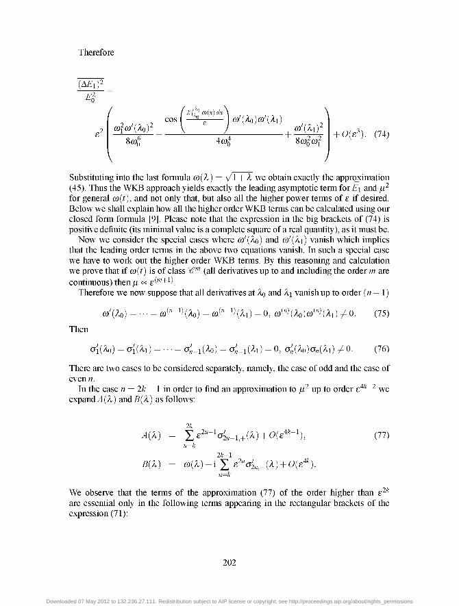
Substituting into the last formula (i){X) = v^T+X we obtain exactly the approximation (45). Thus the WKB approach yields exactly the leading asymptotic term foriii and [J? for general «(/) , and not only that, but also all the higher power terms of e if desired. Below we shall explain how all the higher order WKB terms can be calculated using our closed form formula [9]. Please note that the expression in the big brackets of (74) is positive definite (its minimal value is a complete square of a real quantity), as it must be.

Now we consider the special cases where («'(Ao) and (i)'{X\) vanish which implies that the leading order terms in the above two equations vanish. In such a special case we have to work out the higher order WKB terms. By this reasoning and calculation we prove that if «(/) is of class ' ™ (all derivatives up to and including the order m are continuous) then^ oc e(™+i).

Therefore we now suppose that all derivatives at Ao and X\ vanish up to order (« — 1)

«'(Ao) = = «("-!) (Ao) = «("-i)(Ai) = 0, «W(Ao)«W(î) 7 0. (75)

Then

CTÂo) = C7((Al) = •• • = C7î(Ao) = CTî(Al) = 0, C7^(Ao)c7„(Al) 7^0. (76)

There are two cases to be considered separately, namely, the case of odd and the case of evenw.

In the case « = 2^ — 1 in order to find an approximation to [J? up to order e4*-2 ^g expand^(A) and5(A) as follows:

2k ^(A) Se'"-^cTL_i,+ (A) + 0(e'**+i), (77)

u=k 2k-l

5(A) = « ( A ) - i X e ' " < + ( ^ ) + 0(e u=k

Ak\

We observe that the terms of the approximation (77) of the order higher than e^* are essential only in the following terms appearing in the rectangular brackets of the expression (71):

202


^^^ ^ "-, COS^{-]BI, ^^ ; " \ (78)

sin — cos — - 2 ^ 1-241^1-2 ^ + 2

Taking into account that

2i- l 5(A)2 = «(A)2-2«(A)i X e2«^/^^^(^)^o(g«)^ (79^

BJBJ = a^BJ + co^BJ - COQCO^ + 0 { e * ' ' ) , (80)

and

we easily find:

A{?.)B{?.) = (o{?.)A{?.) + 0{e'"'-') (81)

- 2 < l ^ + 2 ^ ^ 0 ( s - - ) , (82)

2 4 i 5 i _ 2 M l ^ = 0(e«- i )^ (83)

4i - l \ yielding that the coefficient of sin (^) cos (^) in (78) is of the order 0{e ^), and we find

5 5 ^ y i ^ + o„. (5l)Bi + f l " ! ( i ) « . ,84, (OQ V e / (OQ

2 « 2 c o s 2 ( | ) + « 2 s i n 2 ( | ) +

2i- l / „2 \

u=k \ (Oo J

Therefore the expression in the brackets of (71) is equal to

2i- l / 2 2(oi+ X e'" -2«iic7^„,+ (Ai) - 2 i - f c7 „_+(Ao) ) + (85)

u=k \ (Oo '

^ I ; 3 + ^2k-\,+K^) CO, '0

20.1CT-,_,^(^)CT^_,^(AO ^ ^ _ , ^ ^ ^ 7 ( ^ j j ^ ^^ ( , 4 . -1 )

203


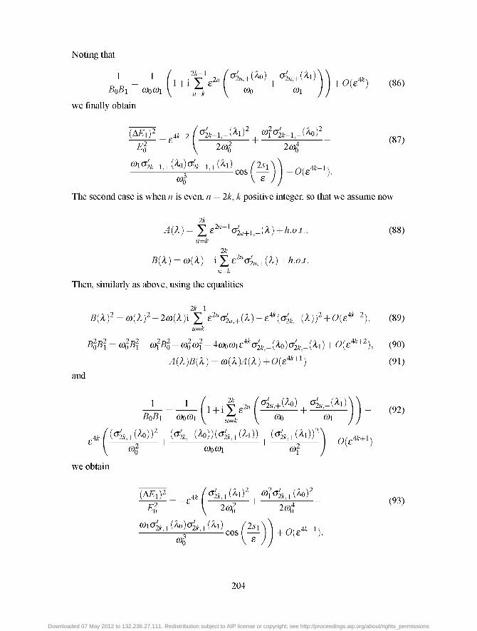
Noting that

1 _ W , , . V . 2 „ ^ < . + W , < . + ( ^ I ) M ,^.„4. l + i Y e^" ^"•+^-^+ ^"•+^ '' +0(8'*^) (86)

we finally obtain

The second case is when n is even, n = 2k,k positive integer, so that we assume now

2k

A{X) = X e2"+i<+i+(A) +/Z.0./., (88) U=k

2k

5(A) = «(A)-iXe'"<+(A)+/^.o./. u=k

Then, similarly as above, using the equalities

2 i - l

BlBJ = (OIB\ + w f s g - (oWi -4o^«ie'**c7^i+(Ao)c7^i,+(Ai) + 0{e^^+^), (90)

^(A)5(A) = «(AM(A) + 0(e'**+i) (91)

and

we obtain

2 r.^2„l

204


We now observe that the expression

^ ^ i < ± ^ M < ± ( M c o s ( f ) ) + 0 ( s - + i ) .

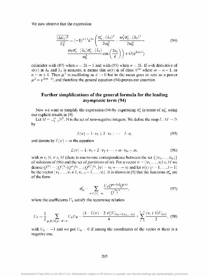
coincides with (87) when n = 2k—\ and with (93) when n = 2k. If «-th derivative of (i){t) at Ao and X\ is nonzero, it means that «(/) is of class ' ™ where m = n—\, or n = m+l. Then ji^ is oscillating as e ^ 0 but in the mean goes to zero as a power ^2 ^ g2(m+i) gjj^ therefore the general equation (94) proves our assertion.

Further simplifications of the general formula for the leading asymptotic term (94)

Now we want to simplify the expression (94) by expressing aj, in terms of co'„, using our explicit results in [9].

Let M = U^^j N*, N is the set of non-negative integers. We define the map L:M ^N by

Z(v) = l-Vi+2-V2 + --- + /-V/ (95)

and denote by Z(v) = /w the equation

Z(v) = 1 • Vi+2-V2H \-m-Vm = m, (96)

with /w G N, V G M (there is one-to-one correspondence between the set {(vi, . . . , Vm)} of solutions of (96) and the set of partitions of m). For a vector v = (vi,.. .,V/) GMwe denote g^^) = (g')" 'iQ'T' • • • [Q^^^Y', |v| = Vi + • • • + V/ and let v(/) (/ = 1 , . . . , / - 1) be the vector (Vl,..., V, + 1 , v,+1 — 1,.. . , V/). It is shown in [9] that the functions cr are of the form

Om= L - 3 ^ ^ ' (97) v:L{v)=m H ^

where the coefficients f/y satisfy the recurrence relation

with UQ = —\ and we put f/a = 0 if among the coordinates of the vector a there is a negative one.

205


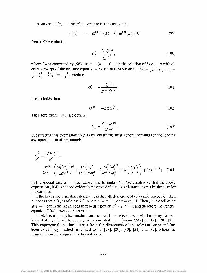
In our case Q{x) = —co^{x). Therefore in the case when

«'(A) = --- = «("-i)(A) = 0, «W(A)7^0 (99)

from (97) we obtain

Q ' (100)

where Uy is computed by (98) and v = (0,. . . ,0,1) is the solution of Z(v) = n with all entries except of the last one equal to zero. From (98) we obtain Uy = 2^^1,0,...,o) = W^{j + 3^0) = -2?H yieding

2"+ig—

If (99) holds then

eW = -2totoW. (102)

Therefore, from (101) we obtain

i"+ito(") "'+ 2" to"

Substituting this expression in (94) we obtain the final general formula for the leading asymptotic term of ji^, namely

(A£i)2

Ei

22«+l 1 2(„+2) (^^)2„^2

(«) («) - 2 ° ^ • cos

^251

V e 2n+U (104)

In the special case « = 1 we recover the formula (74). We emphasize that the above expression (104) is indeed evidently positive definite, which must always be the case for the variance.

If the lowest nonvanishing derivative is the «-th derivative ofco{t) at Ao and/or Ai, then it means that co{t) is of class ' ™ where m = n—I, or n = m+I. Then ji^ is oscillating as e ^ 0 but in the mean goes to zero as a power jj.^ oc e2(m+i) jj j therefore the general equation (104) proves our assertion.

If co{t) is an analytic function on the real time axis {—°°,+°°), the decay to zero is oscillating and on the average is exponential <x Qxp{—const/e) [7], [19], [20], [21]. This exponential smallness stems from the divergence of the relevant series and has been extensively studied in related works [28], [29], [30], [31] and [32], where the resummation techniques have been devised.

206


Let us now summarize our results for the variance ji^ as a function of co{t) embodied in the exact general formulae (70) and (71). If co(t) is analytic between to and ti > to then the equation (104) applies, and as we see ^ is dominated by the switch-on and switch-off events at to and ti, respectively. However, the smaller the lowest nonvanishing derivatives of co{t) at the two points, the smaller will be the power law contribution. Indeed, if to and ti go to —°° and +°°, respectively, and co{t) is analytic on the entire interval, then the behaviour will become exponential at sufficiently large e > EC, whilst it will be oscillatory and in the mean a power law at small e < EC. For example, in figure 5 we observe only exponential regime, because EC is so small.

If there is any non-analyticity of co{t) on this interval, say at ti, then the calculation of jj.^ must be split into two intervals {to,ti) and {ti,ti), calculating the transition matrices for each interval separately, then looking at their product and calculating its matrix elements a,b,c,d, and then proceeding to calculate a + /3 and finally ji^, which will obey a power law like in (104).

In other words, if (i){t) is analytic everywhere, and if the switch-on and switch-off events are completely eliminated, in the sense that they are infinitely smooth, the behaviour of ji^{£) is exponential, as explained above. In all other cases it is a power law.

PERIODIC a)(0

In case when «(/) is periodic with period T but otherwise completely general we can state some general rigorous results. Since the frequency (Oo at time to and (i)\ at time t]_=to + T: are equal, we see from equation (12) due to positive definiteness of ji^ that El is always greater thaniio, that is, in a period T, or any integer multiple of it, T = m, the mean energy E\ never decreases.

If we denote by Oi the transition map (5) for one period of our periodic system, then the transition map 0„ for an interval of exactly n periods of length T is simply a power of Oi, namely

0„ = 0^. (105)

If we use units such that (i)o = (i>\ = I and M = I, then the mean energy from (9) and (10) can be expressed elegantly as the trace of the product of the transition matrix O and its transpose O^, namely

E, = y ( a + /3) = ^[a'+ b^+ 0^+ cf) = | ^ T r ( 0 0 ^ ) . (106)

If O = 0„ = O", then we have to understand the behaviour of the above expression (106) as a function of the number of periods n. This is obviously dictated by the eigenvalues of the transition map Oi, whose determinant is of course equal to I, and its trace is denoted by S, which can be reduced to the diagonal form by a similarity transformation

<i)i = WDW-\ (107)

207


where W is the transformation matrix and D is the diagonal matrix with the eigenvalues ei and €2 = 1/ei, namely the solutions of the quadratic equation for e.

(108)

Therefore ei, €2 = l/e\ are either real reciprocals (if 15*1 > 2) or complex conjugated numbers on the unit circle (if 15*1 < 2). The «-th power of Oi can then be written as

^ = ^„=^\ = WD"W-'^. (109)

Therefore, the matrix elements a,b,c,d of 0„ are bounded when 15*1 < 2 and oscillate with n, while they increase exponentially when 15*1 > 2. Indeed, if ei > 1, then the asymptotic behaviour of (106) is

Ei^KEoe^^, (110)

where ^ is a constant determined by the matrix W in the transformation (107), and the variance at sufficiently large n goes asymptotically as

1 - 9 K--2 M = (A£i)2 « -£2 « _ £ 2 , 4 „ (111)

Therefore, in case when ei > 1, we indeed find that the mean energy and with it the variance of the energy increase exponentially with time T = m, and since (i){t) is bounded, nothing is conserved, ei is determined by 5* = TrOi, and this in turn is determined by the specific properties of the system, that is by the nature of «(/) on the interval (0 ,T) .

So far we discussed the statistical properties of the energy distribution P{E„) in a periodic system. Of course, the contour of the initial uniform canonical ensemble ^ is topologically always a circle, it evolves into the closed curve ^„ after the «-th full period, with the preserved, constant, area enclosed by ^ . This curve is just rotating and oscillating with n in case |TrOi| = 15"! < 2. If 15"! > 2, the action by 0„ = O" is exponentially stretching in the direction of the eigenvector with eigenvalue ei > I, and exponentially contracting in the direction of the other eigenvector with the eigenvalue 62 = I/ei < I. Therefore, the energy of the individual initial condition described by the formula (6) will be exponentially increasing for any initial condition {qo,Po) (vector in the phase plane {q,p)), except for the case when {qo,Po) is exactly in the direction of the second eigenvector (stable manifold) corresponding to 62 = I/ei < I.

GENERAL FORMULA FOR THE ENERGY EVOLUTION

In this section we wish to consider an exact expression for the evolution of the energy distribution by studying a decomposition of one adiabatic process into several consecutive adiabatic processes.

Let us first mention that the energy distributionP{Ei) evolved from the original deltalike distribution 5{E — Eo)isa kind of a Green function for the energy evolution. Let us

208


denote it by G(iii;£'o). If we have a distribution of initial energies w{Eo), such that at each energy EQ the distribution on the energy contour is a uniform canonical distribution, then the final energy distribution is

P{Ei) = j G{Ev,Eo)w{Eo)dEo. (112)

Thus by knowing G, which we call G-function, we can calculate the final energies of any family W{EQ) of uniform canonical ensembles of initial conditions.

If the adiabatic process is ideal adiabatic, then the G-function is a delta function,

G{Ev,Eo) = 5{Ei-(OiEol(Oo). (113)

For ensembles of other types, which are not uniform canonical, we must go back to our fundamental equation (8) and perform the averaging using the distribution in space (i?o,</)).

Now suppose that the interval of length T is divided into an arbitrary number of finite subintervals {tj,tj+\), where to is the beginning of the process (interval) and t„ is the end of the process, and 7 = 0,1,.. . ,« — 1. The behaviour of «(/) inside each j-th subinterval is assumed to be entirely arbitrary, but the process must be such that at each integration step tj the distribution is uniform canonical. This condition is certainly satisfied if the process is ideal adiabatic, in general not.

It is then obvious that the energy G-function G{E;EQ) for the complete process divided into n subintervals is given by the multiple integral

G{E;Eo)= / . . . / G „ ( £ ; X „ _ I ) G „ _ I ( x„_i;x„_2) • • • G\[X\',EQ)CIX„_\ .. .clx2dx\. (114)

n - l

Indeed, using (113) we can immediately verily this equation. All moments of the final distribution can be easily calculated as they are all fully determined by the first moment alone, so what we need is just the first moment. From our theory in section 2 we know that in full generality the first moment of any G{E; iio) is a linear function of the initial value Eo, namely

E= l'EG{E;Eo)dE=gEo, (115)

where the constant g = (a + /3 )/2 is a constant independent of iio and is determined by the nature ofco{t) inside the relevant interval of evolution. We shall call g the g-factor of G. For an ideal adiabatic process we know from (13) thatgy = coj/coj^i. From equation (114) we immediately find the factorization property

g = gngn-l---g2gl, E=gEo=g„...g2glEo. (116)

Obviously, for an ideal adiabatic process where eachgy = coj/coj-i, the above equation is certainly satisfied.

209


It is possible also to show the converse [24]: If the composition formula (114) is true for any intermediate points of integration tj and xj, then the process must be ideal adiabatic, implying that

G{Ej;Ej_r) = 8{Ej - (OjEj^r/oij-i) (117)

applies for all j , and gj = coj/coj-i. This can be shown by splitting the time interval {to,t„) into infinitesimal subintervals and using a piecewise constant function to approximate co{t), and then using gj = ^{coJ/coJ_^ + 1) from equation (24) for all j , finally evaluating g by equation (116), and finding g= co„/coo, which implies that the process is ideal adiabatic at all times of the time interval, because ^^ = 0.

The composition formula (114) (factorization property of the G-function) will apply also in nonlinear systems, but the relationship between Ei and EQ is then no longer linear Therefore using the composition formula (114) for infinitesimal intervals, and approximating co{t) by piecewise constant or piecewise hnear functions etc. might be of extreme importance to find new global powerful approximations for G-functions and their moments.

The theory for nonlinear systems is left open for the future work.

DISCUSSION AND CONCLUSIONS

The purpose of this paper is to review the ideas, methods and results of the series of our papers [1, 2, 3] on the dynamics of a time-dependent linear oscillator, where the oscillation frequency co{t) is an arbitrary function of time. External forcing can be analyzed in a similar way, but could not be covered due to the lack of space, but the interested reader should see the paper [4].

We have studied the evolution of the energy of such a system over a time interval of length T, and also its statistical properties, in particular the distribution function P{Ei) of the final energies Ei under the assumption that the initial ensemble of initial conditions is a uniform canonical ensemble of initial conditions (i.e. uniform w.rt. the angle variables) ^ at the sharply defined initial energy EQ. The crucial point is that for the linear oscillator we know the phase flow or the so-caUed transition map exphcitly in the form of a 2 x 2 matrix. Using this, we can explicitly calculate the distribution

function P(x) = n^^(2ji^ —x^)^^, where x = Ei —Ei, and Ei and ji^ are the final average energy and variance, respectively. Thus the distribution function is universal, and this result is exact and rigorous. In nonlinear time-dependent oscfllators the main and major difficulty is that we do not know the phase flow globally, and consequently we can not perform averages of the final quantities in terms of the initial conditions. Practically all perturbation schemes break down at finite time, so asymptotic results T ^oo cannot be obtained in an easy way.

In case of A = 1 this is also microcanonical ensemble, in terminology of statistical mechanics, unlike the case of higher dimensional tori N >2, which we do not analyze here.

210


We are able to calculate rigorously all the moments of P(i?i). Odd moments are exactly zero, the even moments are powers of the second moment ji^. The latter one is a_function of the first moment. Therefore everything is determined by the first moment El. In order to calculate Ei and ji^ etc. we can use the WKB method as developed in our paper [9], and explained in detail in the present paper

In our analysis we clearly see when the adiabatic invariant I{t) = E{t)/co{t) is conserved or not. In the (ideal) adiabatic limit T ^ oo it is conserved, the variance ji^ is zero andiii = Ei = COIEQ/COO, andP(i?i) is a delta function P(iii) = 5{Ei—Ei). If it is not conserved exactly, when T is finite, we find ji^ = E^[{Ei/Eo)^ - {a){T)/a){0))^]/2 > 0, and it can be calculated using a WKB method analytically in a closed form, which is a major achievement of our work. From this follows^at once the conclusion that the adiabatic invariant I = Ei/(Oi at the average energy Ei never decreases, which is a kind of irreversibility statement.

We have also studied three specific solvable models and have demonstrated the power of the WKB expansion, where already the leading WKB term usually very well describes the asymptotic behaviour of ^^ when e = \/T goes to zero. We also show what happens if (i){t) is smooth and of class ' ™, having m continuous derivatives, calculating and showing that fi^ oscillates as e goes to zero, but in the mean vanishes as o e2(™+i) if (i){t) is analytic, thus it also is of class '^°°, it is known from the literature that ji^ must decay exponentially <x Qxp{const/e). lfco{t) is periodic, Ei can grow exponentially, and so does the variance ji^, in which case I{t) = E{t)/co{t) is not conserved, but we can describe the system.

We have introduced the so-called G-function, which is a kind of a Green function for the evolution of the energy and derived a composition formula for it when the interval of evolution is decomposed into a finite number of subintervals, for which the corresponding Gy-function is known for all subintervals j and is uniform canonical there. This formula applies also to nonlinear systems and might be a good starting basis to describe them. The theory for nonlinear systems remains open and is a subject of the current research [24].

ACKNOWLEDGMENTS

The collaboration on topics of paper [4] with Dr Audrey V. Kuzmin, concerning the arbitrary external forcing of a time-dependent hnear oscillator, is not included in this review due to lack of space, but is greatfully acknowledged. The authors acknowledge the support of the Slovenian Research Agency, the Nova Kreditna Banka Maribor, and the TELEKOM Slovenije.

REFERENCES

1. M. Robnik, and V. G. Romanovski, J. Phys. A: Math. Gen. 39, L35 (2006). 2. M. Robnik, and V. G. Romanovski, OpenSyst & InformationDyn. 13, 197 (2006). 3. M. Robnik, V. G. Romanovski, and H.-J. Stockmann, J. Phys. A: Math. Gen. 39, L551 (2006). 4. A. V. Kuzmin, and M. Robnik, Reports on Mathematical Physics 60, 69 (2007). 5. A. Einstein, Inst intern, pitys. Solway, Rapports et discussions 1, 450 (1911).

211


6. M. Robnik, Encyclopedia of Nonlinear Science, Ed. A. Scott, Routledge, New York, 2005, pp. 2-5. 7. L. D. Landau, and E. M. IMsbiitL, Mechanics: Course of Theoretical Physics, Butterworth-Heineman,

Oxford, 1996. 8. W. R Reinhardt, Prog. Theor Phys Suppl 116, 179 (1994). 9. M. Robnik, and V. G. Romanovski, J. Phys A: Math. Gen. 33, 5093 (2000). 10. R. M. Kulsrud, Phys Rev. 106, 205 (1957). 11. H. Hertweck, and A. SchMer, Zeitschriftf Natuiforschung 12 A, 844(1957). 12. C. S. Gardner, Phys Rev. 115, 791 (1959). 13. A. Lenard, Ann. Phys, NY 6, 261 (1959). 14. E. D. Courant, and H. S. Snyder, Ann. Phys, NY 3, 1 (1958). 15. J. E. Littlewood,^««. Phys., NY 21, 223 (1963). 16. M. Kruskal, J. Math Phys 3, 806 (1962). 17. H. R. Lewis, J. Math Phys 9, 1976 (1968). 18. H. R. Lewis, J. Math Phys 11, 1320 (1970). 19. G. Knorr, and D. Pfirsch, Zeitschriftf Naturforschung 21, 688 (1966). 20. R. E. Meyer, Z. Angew. Math Phys 24, 293 (1973). 21. R. E. Meyer, Z. Angew. Math Phys 24, 517 (1973). 22. I. S. Gradshteyn, and I. M. Ryzhik, Table oflntegrals. Series andProducts, ED. A. Jeffrey, Academic,

SanDiago, CA, 1994. 23. W. Feller, An Introduction to Probability Theory and its Applications Vol II, Wiley, New York, 1971. 24. M. Robnik, and V. G. Romanovski, in preparation (2008). 25. M. Robnik, and T. A. Wood, NonlinearPhenom. in ComplexSyst 9, 141 (2006). 26. M. Abramowitz, and I. A. ^iXegun, Handbook of Mathematical Functions, Dover, New York, 1972. 27. N. Vmman,Arkivf6rPhysiki2, 541 (1966). 28. M. V. Berry, J Phys A: Math. Gen 15, 3693 (1982). 29. M. V. Berry, Proc. Roy Soc Lond A 429, 61 (1990). 30. A. Joye, J Phys A: Math Gen. 26, 6517 (1993). 31. A. Joye, H. Kunz, and C.-E. Pfister,^««. Phys NY 208, 299 (1991). 32. R. Lim, and M. V. Berry, J Phys A: Math Gen. 24, 3255 (1991).

212


[AIP LET’S FACE CHAOS THROUGH NONLINEAR DYNAMICS: Proceedings of “Let’s Face Chaos Through...

Documents

Transcript of [AIP LET’S FACE CHAOS THROUGH NONLINEAR DYNAMICS: Proceedings of “Let’s Face Chaos Through...