Aim of Lesson Objectives - University of Toledo · Lesson 4: Radiometric correction of satellite...
23
Lesson 4: Radiometric correction of satellite images 4: RADIOMETRIC CORRECTION OF SATELLITE IMAGES: WHEN AND WHY RADIOMETRIC CORRECTION IS NECESSARY Aim of Lesson To develop your understanding of concepts underlying radiometric correction and how to carry out the radiometric correction of satellite imagery, using two Landsat Thematic Mapper images obtained at different seasons under different atmospheric conditions as examples. Objectives 1. To understand the difference between DN values, radiance and reflectance. 2. To understand why radiometric correction of imagery is required if (i) you are mapping changes in habitat or other features, or (ii) you are using more than one image in a study. 3. To demonstrate how different atmospheric conditions can affect DN values by comparing these in two Landsat TM images acquired during different seasons. 4. To understand the basic concepts behind atmospheric correction algorithms. 5. To learn how to carry out the process of radiometric correction of two Landsat TM images obtained in different seasons and compare the resultant reflectance values. Background Information This lesson relates to material covered in Chapter 7 of the Remote Sensing Handbook for Tropical Coastal Management and readers are recommended to consult this for further details of the techniques involved. The lesson is rather a specialist one designed to guide practitioners in radiometric and atmospheric correction; it is advanced and is quite hard work (be warned!). Atmospheric correction will be carried out on two Landsat Thematic Mapper images of the Caicos Bank obtained at different seasons and under somewhat different atmospheric conditions. The first Landsat TM image was acquired in November 1990 whilst the second image (simulated) is for the rather different atmospheric conditions and sun elevation of June 1990. At the time of the November overpass horizontal visibility was estimated at 35 km whilst for the June one it was only 20 km. The sun elevation angle for the winter overpass was 39° but that for the summer overpass was 58°. The DN values recorded for the same areas of the Earth’s surface thus differ considerably between the two images. The Bilko 3 image processing software Familiarity with Bilko is required to carry out this lesson. In particular, you will need experience of using Formula documents to carry out mathematical manipulations of images and should be familiar with creating colour composites and reading off pixel values from the status bar. These features are covered in Tutorials 10, 2 and 3 respectively of the Introduction to using the Bilko 3 image processing software. A familiarity with the Microsoft Excel spreadsheet package is also desirable because some calculations need to be performed independently; these can either be carried out on a spreadsheet or using a calculator. Image data The first image was acquired by Landsat-5 TM on 22 November 1990 at 14.55 hours Universal Time (expressed as a decimal time and thus equivalent to 14:33 GMT). The Turks & Caicos Islands are on GMT – 5 hours so the overpass would have been at 09:33 local time. You are provided with bands #1 1
Transcript of Aim of Lesson Objectives - University of Toledo · Lesson 4: Radiometric correction of satellite...
Lesson 4: Radiometric correction of satellite images
4: RADIOMETRIC CORRECTION OF SATELLITE IMAGES: WHEN AND WHY RADIOMETRIC CORRECTION IS NECESSARY
Aim of Lesson To develop your understanding of concepts underlying radiometric correction and how to carry out the radiometric correction of satellite imagery, using two Landsat Thematic Mapper images obtained at different seasons under different atmospheric conditions as examples.
Objectives 1. To understand the difference between DN values, radiance and reflectance.
2. To understand why radiometric correction of imagery is required if (i) you are mapping changes in habitat or other features, or (ii) you are using more than one image in a study.
3. To demonstrate how different atmospheric conditions can affect DN values by comparing these in two Landsat TM images acquired during different seasons.
4. To understand the basic concepts behind atmospheric correction algorithms.
5. To learn how to carry out the process of radiometric correction of two Landsat TM images obtained in different seasons and compare the resultant reflectance values.
Background Information This lesson relates to material covered in Chapter 7 of the Remote Sensing Handbook for Tropical Coastal Management and readers are recommended to consult this for further details of the techniques involved. The lesson is rather a specialist one designed to guide practitioners in radiometric and atmospheric correction; it is advanced and is quite hard work (be warned!).
Atmospheric correction will be carried out on two Landsat Thematic Mapper images of the Caicos Bank obtained at different seasons and under somewhat different atmospheric conditions. The first Landsat TM image was acquired in November 1990 whilst the second image (simulated) is for the rather different atmospheric conditions and sun elevation of June 1990. At the time of the November overpass horizontal visibility was estimated at 35 km whilst for the June one it was only 20 km. The sun elevation angle for the winter overpass was 39° but that for the summer overpass was 58°. The DN values recorded for the same areas of the Earth’s surface thus differ considerably between the two images.
The Bilko 3 image processing software Familiarity with Bilko is required to carry out this lesson. In particular, you will need experience of using Formula documents to carry out mathematical manipulations of images and should be familiar with creating colour composites and reading off pixel values from the status bar. These features are covered in Tutorials 10, 2 and 3 respectively of the Introduction to using the Bilko 3 image processing software. A familiarity with the Microsoft Excel spreadsheet package is also desirable because some calculations need to be performed independently; these can either be carried out on a spreadsheet or using a calculator.
Image data The first image was acquired by Landsat-5 TM on 22 November 1990 at 14.55 hours Universal Time (expressed as a decimal time and thus equivalent to 14:33 GMT). The Turks & Caicos Islands are on GMT – 5 hours so the overpass would have been at 09:33 local time. You are provided with bands #1
1
Applications of satellite and airborne image data to coastal management
(blue), #2 (green) and #3 (red) of this image as the files LandsatTM_Nov_DN#01.gif, LandsatTM_Nov_DN#02.gif and LandsatTM_Nov_DN#03.gif. These images are of DN values but have been geometrically corrected. The second Landsat-5 TM image has been simulated for the rather different atmospheric conditions and sun elevation of 22 June 1990 at 14.55 hours Universal Time by the reverse of the process you are learning to carry out in this lesson (i.e. surface reflectance values have been converted to DN values at the sensor). You are provided with bands #1 (blue), #2 (green) and #3 (red) of this image as the files LandsatTM_Jun_DN#01.gif, LandsatTM_Jun_DN#02.gif and LandsatTM_Jun_DN#03.gif. These images are also of DN values and have been geometrically corrected so that pixels can be compared between seasons. The centre of each scene is at 21.68° N and 72.29° W.
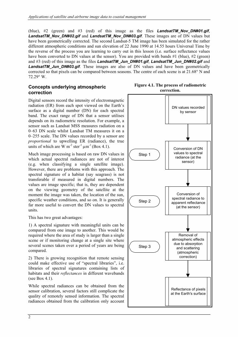
Figure 4.1. The process of radiometric correction.
Concepts underlying atmospheric correction
Conversion of DNvalues to spectralradiance (at the
sensor)
Conversion ofspectral radiance toapparent reflectance
(at the sensor)
Removal ofatmospheric effectsdue to absorption
and scattering(atmosphericcorrection)
DN values recordedby sensor
Reflectance of pixelsat the Earth's surface
Step 1
Step 3
Step 2
Digital sensors record the intensity of electromagnetic radiation (ER) from each spot viewed on the Earth’s surface as a digital number (DN) for each spectral band. The exact range of DN that a sensor utilises depends on its radiometric resolution. For example, a sensor such as Landsat MSS measures radiation on a 0–63 DN scale whilst Landsat TM measures it on a 0–255 scale. The DN values recorded by a sensor are proportional to upwelling ER (radiance), the true units of which are W m-2 ster-1 µm-1 (Box 4.1).
Much image processing is based on raw DN values in which actual spectral radiances are not of interest (e.g. when classifying a single satellite image). However, there are problems with this approach. The spectral signature of a habitat (say seagrass) is not transferable if measured in digital numbers. The values are image specific; that is, they are dependent on the viewing geometry of the satellite at the moment the image was taken, the location of the sun, specific weather conditions, and so on. It is generally far more useful to convert the DN values to spectral units.
This has two great advantages:
1) A spectral signature with meaningful units can be compared from one image to another. This would be required where the area of study is larger than a single scene or if monitoring change at a single site where several scenes taken over a period of years are being compared.
2) There is growing recognition that remote sensing could make effective use of “spectral libraries”, i.e. libraries of spectral signatures containing lists of habitats and their reflectances in different wavebands (see Box 4.1).
While spectral radiances can be obtained from the sensor calibration, several factors still complicate the quality of remotely sensed information. The spectral radiances obtained from the calibration only account
2

Lesson 4: Radiometric correction of satellite images
for the spectral radiance measured at the satellite sensor. By the time ER is recorded by a satellite or airborne sensor, it has already passed through the Earth’s atmosphere twice (sun to target and target to sensor).
Figure 4.2. Simplified schematic of atmospheric interference and the passage of electromagnetic radiation from the Sun to the satellite sensor.
During this passage (Figure 4.2), the radiation is affected by two processes: absorption, which reduces its intensity, and scattering, which alters its direction. Absorption occurs when electromagnetic radiation interacts with gases such as water vapour, carbon dioxide and ozone. Scattering results from interactions between ER and both gas molecules and airborne particulate matter (aerosols). These molecules and particles range in size from the raindrop (>100 µm) to the microscopic (<1 µm). Scattering will redirect incident electromagnetic radiation and deflect reflected ER from its path (Figure 4.2).
Box 4.1. Units of electromagnetic radiation
The unit of electromagnetic radiation is W m-2 ster-1 µm-1. That is, the rate of transfer of energy (Watt, W) recorded at a sensor, per square metre on the ground, for one steradian (three dimensional angle from a point on Earth’s surface to the sensor), per unit wavelength being measured. This measure is referred to as the spectral radiance. Prior to the launch of a sensor, the relationship between measured spectral radiance and DN is determined. This is known as the sensor calibration. It is worth clarifying terminology at this point. The term radiance refers to any radiation leaving the Earth (i.e. upwelling, toward the sensor). A different term, irradiance, is used to describe downwelling radiation reaching the Earth from the sun (Figure 4.2). The ratio of upwelling to downwelling radiation is known as reflectance. Reflectance does not have units and is measured on a scale from 0 to 1 (or 0–100%).
Absorption and scattering create an overall effect of “haziness” which reduces the contrast in the image. Scattering also creates the “adjacency effect” in which the radiance recorded for a given pixel partly incorporates the scattered radiance from neighbouring pixels.
3
Applications of satellite and airborne image data to coastal management
In order to make a meaningful measure of radiance at the Earth’s surface, the atmospheric interferences must be removed from the data. This process is called “atmospheric correction”. The entire process of radiometric correction involves three steps (Figure 4.1).
The spectral radiance of features on the ground is usually converted to reflectance. This is because spectral radiance will depend on the degree of illumination of the object (i.e. the irradiance). Thus spectral radiances will depend on such factors as time of day, season, latitude, etc. Since reflectance represents the ratio of radiance to irradiance, it provides a standardised measure that is directly comparable between images.
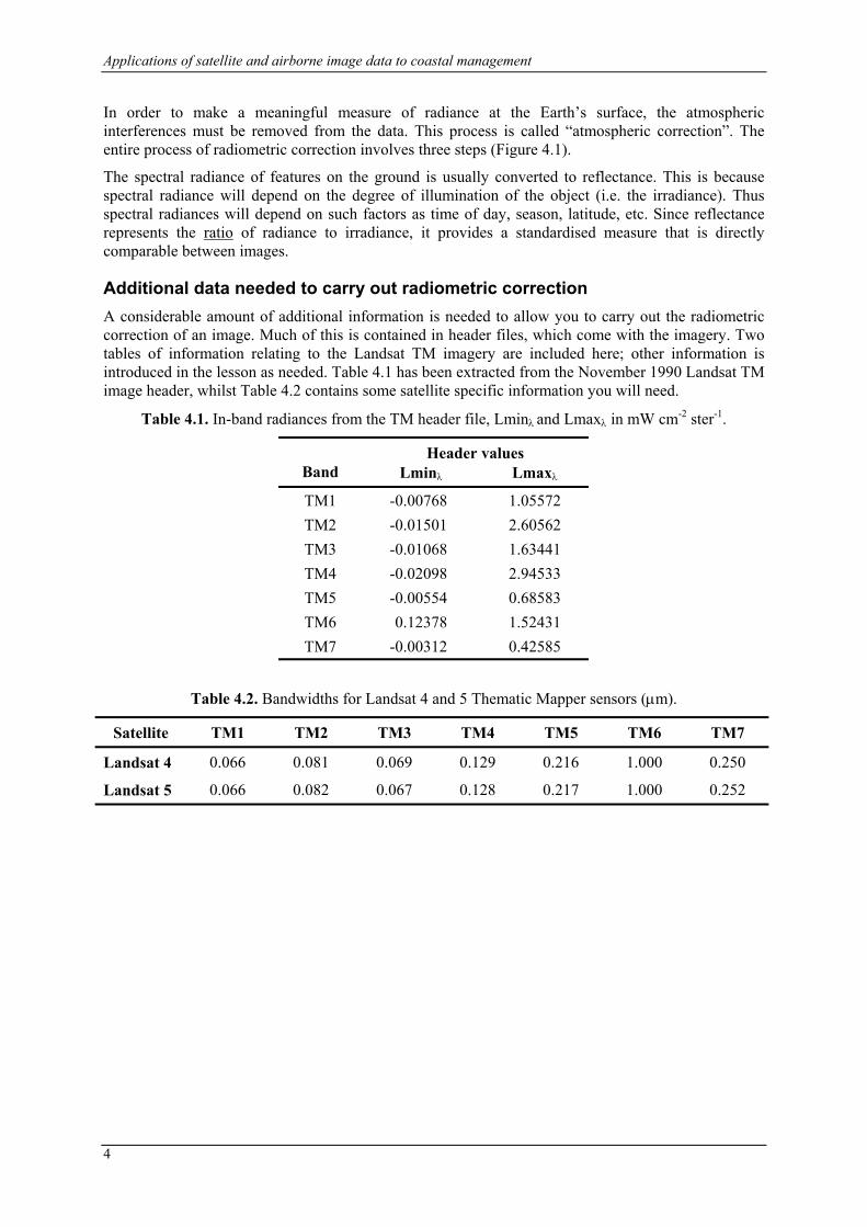
Additional data needed to carry out radiometric correction A considerable amount of additional information is needed to allow you to carry out the radiometric correction of an image. Much of this is contained in header files, which come with the imagery. Two tables of information relating to the Landsat TM imagery are included here; other information is introduced in the lesson as needed. Table 4.1 has been extracted from the November 1990 Landsat TM image header, whilst Table 4.2 contains some satellite specific information you will need.
Table 4.1. In-band radiances from the TM header file, Lminλ and Lmaxλ in mW cm-2 ster-1.
Header values Band Lminλ Lmaxλ
TM1 -0.00768 1.05572 TM2 -0.01501 2.60562 TM3 -0.01068 1.63441 TM4 -0.02098 2.94533 TM5 -0.00554 0.68583 TM6 0.12378 1.52431 TM7 -0.00312 0.42585
Table 4.2. Bandwidths for Landsat 4 and 5 Thematic Mapper sensors (µm).
Satellite TM1 TM2 TM3 TM4 TM5 TM6 TM7
Landsat 4 0.066 0.081 0.069 0.129 0.216 1.000 0.250
Landsat 5 0.066 0.082 0.067 0.128 0.217 1.000 0.252
4
Lesson 4: Radiometric correction of satellite images
Lesson Outline
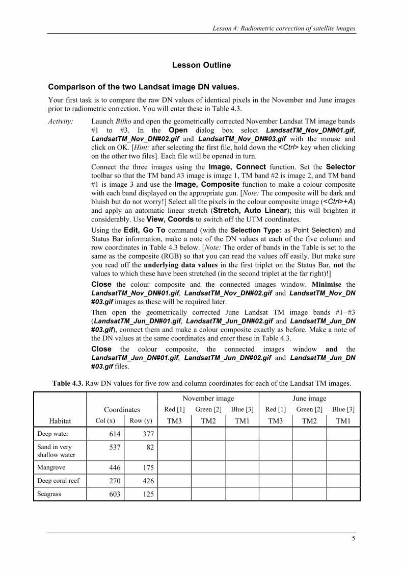
Comparison of the two Landsat image DN values. Your first task is to compare the raw DN values of identical pixels in the November and June images prior to radiometric correction. You will enter these in Table 4.3.
Activity: Launch Bilko and open the geometrically corrected November Landsat TM image bands #1 to #3. In the Open dialog box select LandsatTM_Nov_DN#01.gif, LandsatTM_Nov_DN#02.gif and LandsatTM_Nov_DN#03.gif with the mouse and click on OK. [Hint: after selecting the first file, hold down the <Ctrl> key when clicking on the other two files]. Each file will be opened in turn.
Connect the three images using the Image, Connect function. Set the Selector toolbar so that the TM band #3 image is image 1, TM band #2 is image 2, and TM band #1 is image 3 and use the Image, Composite function to make a colour composite with each band displayed on the appropriate gun. [Note: The composite will be dark and bluish but do not worry!] Select all the pixels in the colour composite image (<Ctrl>+A) and apply an automatic linear stretch (Stretch, Auto Linear); this will brighten it considerably. Use View, Coords to switch off the UTM coordinates.
Using the Edit, Go To command (with the Selection Type: as Point Selection) and Status Bar information, make a note of the DN values at each of the five column and row coordinates in Table 4.3 below. [Note: The order of bands in the Table is set to the same as the composite (RGB) so that you can read the values off easily. But make sure you read off the underlying data values in the first triplet on the Status Bar, not the values to which these have been stretched (in the second triplet at the far right)!]
Close the colour composite and the connected images window. Minimise the LandsatTM_Nov_DN#01.gif, LandsatTM_Nov_DN#02.gif and LandsatTM_Nov_DN #03.gif images as these will be required later.
Then open the geometrically corrected June Landsat TM image bands #1– #3 (LandsatTM_Jun_DN#01.gif, LandsatTM_Jun_DN#02.gif and LandsatTM_Jun_DN #03.gif), connect them and make a colour composite exactly as before. Make a note of the DN values at the same coordinates and enter these in Table 4.3.
Close the colour composite, the connected images window and the LandsatTM_Jun_DN#01.gif, LandsatTM_Jun_DN#02.gif and LandsatTM_Jun_DN #03.gif files.
Table 4.3. Raw DN values for five row and column coordinates for each of the Landsat TM images.
November image June image Coordinates Red [1] Green [2] Blue [3] Red [1] Green [2] Blue [3]
Habitat Col (x) Row (y) TM3 TM2 TM1 TM3 TM2 TM1
Deep water 614 377
Sand in very shallow water
537 82
Mangrove 446 175
Deep coral reef 270 426
Seagrass 603 125
5
Applications of satellite and airborne image data to coastal management
Question: 4.1. Why do you think the Landsat TM3 DN value for the deep water and for the deep coral reef area is the same?
Question: 4.2. Why do you think the Landsat TM3 DN value for the shallow seagrass area is almost the same as that for deep water and deep coral reef?
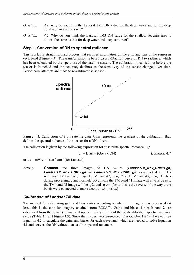
Step 1. Conversion of DN to spectral radiance This is a fairly straightforward process that requires information on the gain and bias of the sensor in each band (Figure 4.3). The transformation is based on a calibration curve of DN to radiance, which has been calculated by the operators of the satellite system. The calibration is carried out before the sensor is launched and the accuracy declines as the sensitivity of the sensor changes over time. Periodically attempts are made to re-calibrate the sensor.
Figure 4.3. Calibration of 8-bit satellite data. Gain represents the gradient of the calibration. Bias defines the spectral radiance of the sensor for a DN of zero.
The calibration is given by the following expression for at satellite spectral radiance, Lλ:
Lλ = Bias + (Gain x DN) Equation 4.1
units: mW cm-2 ster-1 µm-1 (for Landsat)
Activity: Connect the three images of DN values (LandsatTM_Nov_DN#01.gif, LandsatTM_Nov_DN#02.gif and LandsatTM_Nov_DN#03.gif) as a stacked set. This will make TM band #1, image 1; TM band #2, image 2; and TM band #3, image 3. Thus during processing using Formula documents the TM band #1 image will always be @1, the TM band #2 image will be @2, and so on. [Note: this is the reverse of the way these bands were connected to make a colour composite.]
Calibration of Landsat TM data The method for calculating gain and bias varies according to when the imagery was processed (at least, this is the case for imagery obtained from EOSAT). Gains and biases for each band λ are calculated from the lower (Lminλ) and upper (Lmaxλ) limits of the post-calibration spectral radiance range (Table 4.1 and Figure 4.3). Since the imagery was processed after October 1st 1991 we can use Equation 4.2 to calculate the gains and biases for each waveband, which are needed to solve Equation 4.1 and convert the DN values to at satellite spectral radiances.
6
Lesson 4: Radiometric correction of satellite images
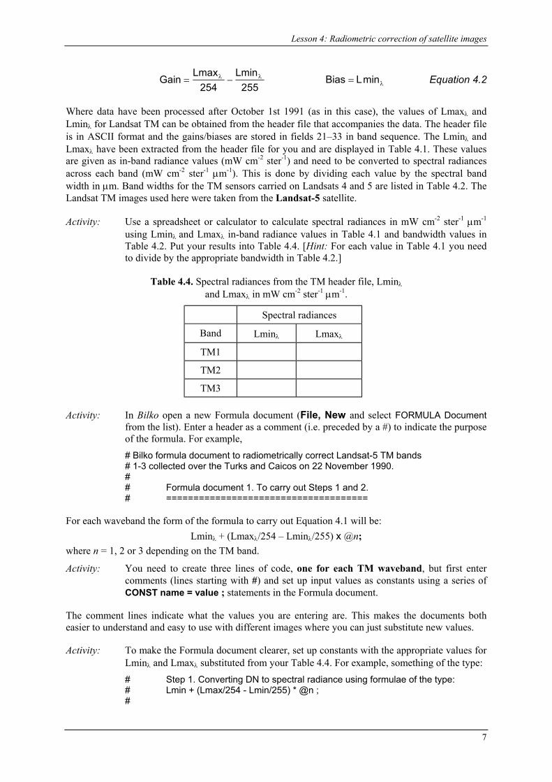
GainLmax
254Lmin
255= −λ λ Equation 4.2 Bias L= minλ
Where data have been processed after October 1st 1991 (as in this case), the values of Lmaxλ and Lminλ for Landsat TM can be obtained from the header file that accompanies the data. The header file is in ASCII format and the gains/biases are stored in fields 21–33 in band sequence. The Lminλ and Lmaxλ have been extracted from the header file for you and are displayed in Table 4.1. These values are given as in-band radiance values (mW cm-2 ster-1) and need to be converted to spectral radiances across each band (mW cm-2 ster-1 µm-1). This is done by dividing each value by the spectral band width in µm. Band widths for the TM sensors carried on Landsats 4 and 5 are listed in Table 4.2. The Landsat TM images used here were taken from the Landsat-5 satellite.
Activity: Use a spreadsheet or calculator to calculate spectral radiances in mW cm-2 ster-1 µm-1 using Lminλ and Lmaxλ in-band radiance values in Table 4.1 and bandwidth values in Table 4.2. Put your results into Table 4.4. [Hint: For each value in Table 4.1 you need to divide by the appropriate bandwidth in Table 4.2.]
Table 4.4. Spectral radiances from the TM header file, Lminλ
and Lmaxλ in mW cm-2 ster-1 µm-1.
Spectral radiances
Band Lminλ Lmaxλ
TM1
TM2
TM3
Activity: In Bilko open a new Formula document (File, New and select FORMULA Document from the list). Enter a header as a comment (i.e. preceded by a #) to indicate the purpose of the formula. For example,
# Bilko formula document to radiometrically correct Landsat-5 TM bands # 1-3 collected over the Turks and Caicos on 22 November 1990.
# # Formula document 1. To carry out Steps 1 and 2. # =====================================
For each waveband the form of the formula to carry out Equation 4.1 will be: Lminλ + (Lmaxλ/254 – Lminλ/255) x @n;
where n = 1, 2 or 3 depending on the TM band.
Activity: You need to create three lines of code, one for each TM waveband, but first enter comments (lines starting with #) and set up input values as constants using a series of CONST name = value ; statements in the Formula document.
The comment lines indicate what the values you are entering are. This makes the documents both easier to understand and easy to use with different images where you can just substitute new values.
Activity: To make the Formula document clearer, set up constants with the appropriate values for Lminλ and Lmaxλ substituted from your Table 4.4. For example, something of the type:
# Step 1. Converting DN to spectral radiance using formulae of the type: # Lmin + (Lmax/254 - Lmin/255) * @n ; #
7
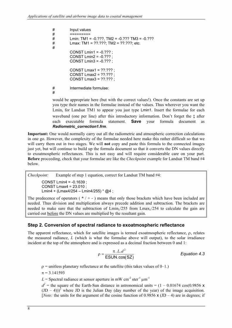
Applications of satellite and airborne image data to coastal management
# Input values # ========= # Lmin: TM1 = -0.???, TM2 = -0.??? TM3 = -0.??? # Lmax: TM1 = ??.???; TM2 = ??.???; etc. # CONST Lmin1 = -0.??? ; CONST Lmin2 = -0.??? ; CONST Lmin3 = -0.??? ; CONST Lmax1 = ??.??? ; CONST Lmax2 = ??.??? ; CONST Lmax3 = ??.??? ; # Intermediate formulae: #
would be appropriate here (but with the correct values!). Once the constants are set up you type their names in the formulae instead of the values. Thus wherever you want the Lminλ for Landsat TM1 to appear you just type Lmin1. Insert the formulae for each waveband (one per line) after this introductory information. Don’t forget the ; after each executable formula statement. Save your formula document as Radiometric_correction1.frm.
Important: One would normally carry out all the radiometric and atmospheric correction calculations in one go. However, the complexity of the formulae needed here make this rather difficult so that we will carry them out in two stages. We will not copy and paste this formula to the connected images just yet, but will continue to build up the formula document so that it converts the DN values directly to exoatmospheric reflectances. This is not easy and will require considerable care on your part. Before proceeding, check that your formulae are like the Checkpoint example for Landsat TM band #4 below.
Checkpoint: Example of step 1 equation, correct for Landsat TM band #4: CONST Lmin4 = -0.1639 ; CONST Lmax4 = 23.010 ; Lmin4 + (Lmax4/254 – Lmin4/255) * @4 ;
The predecence of operators ( * / + - ) means that only those brackets which have been included are needed. Thus division and multiplication always precede addition and subtraction. The brackets are needed to make sure that the subtraction of Lminλ/255 from Lmaxλ/254 to calculate the gain are carried out before the DN values are multiplied by the resultant gain.
Step 2. Conversion of spectral radiance to exoatmospheric reflectance
The apparent reflectance, which for satellite images is termed exoatmospheric reflectance, ρ, relates the measured radiance, L (which is what the formulae above will output), to the solar irradiance incident at the top of the atmosphere and is expressed as a decimal fraction between 0 and 1:
( )
ρπ
=. L d.
ESUN.cos SZ
2
Equation 4.3
ρπ
= unitless planetary reflectance at the satellite (this takes values of 0–1.) = 3.141593
L = Spectral radiance at sensor aperture in mW cm-2 ster-1 µm-1 d2 = the square of the Earth-Sun distance in astronomical units = (1 – 0.01674 cos(0.9856 x (JD – 4)))2 where JD is the Julian Day (day number of the year) of the image acquisition. [Note: the units for the argument of the cosine function of 0.9856 x (JD – 4) are in degrees; if
8
Lesson 4: Radiometric correction of satellite images
your cosine function (e.g. the cos function in Excel is expecting the argument in radians, multiply by π/180 before taking the cosine).] ESUN = Mean solar exoatmospheric irradiance in mW cm-2 µm-1. ESUN can be obtained from Table 4.5. SZ = sun zenith angle when the scene was recorded. Note: The Bilko formula expects this argument in radians.
Both Landsat and SPOT products provide sun elevation angle. The zenith angle (SZ) is calculated by subtracting the sun elevation from 90° (π/2 radians).
Activity: Calculate the Julian Day (day number of the year) of the image acquisition. The date of acquisition can be found in the Image data section above. A quick way to do this is to enter the date of acquisition in one cell of an Excel spreadsheet and the date of the end of the previous year (e.g. 31 December 1989) in another cell. Then enter a formula in a next door cell which subtracts the second date from the first. Thus, 1 January 1990 is day 1, etc.
Having calculated the Julian Day (JD), work out the square of the Earth-Sun distance in astronomical units (d²) using the equation above. Use a spreadsheet or calculator.
The sun elevation angle at the time the scene was recorded was 39°. Calculate the sun zenith angle in degrees for when the scene was recorded and convert to radians.
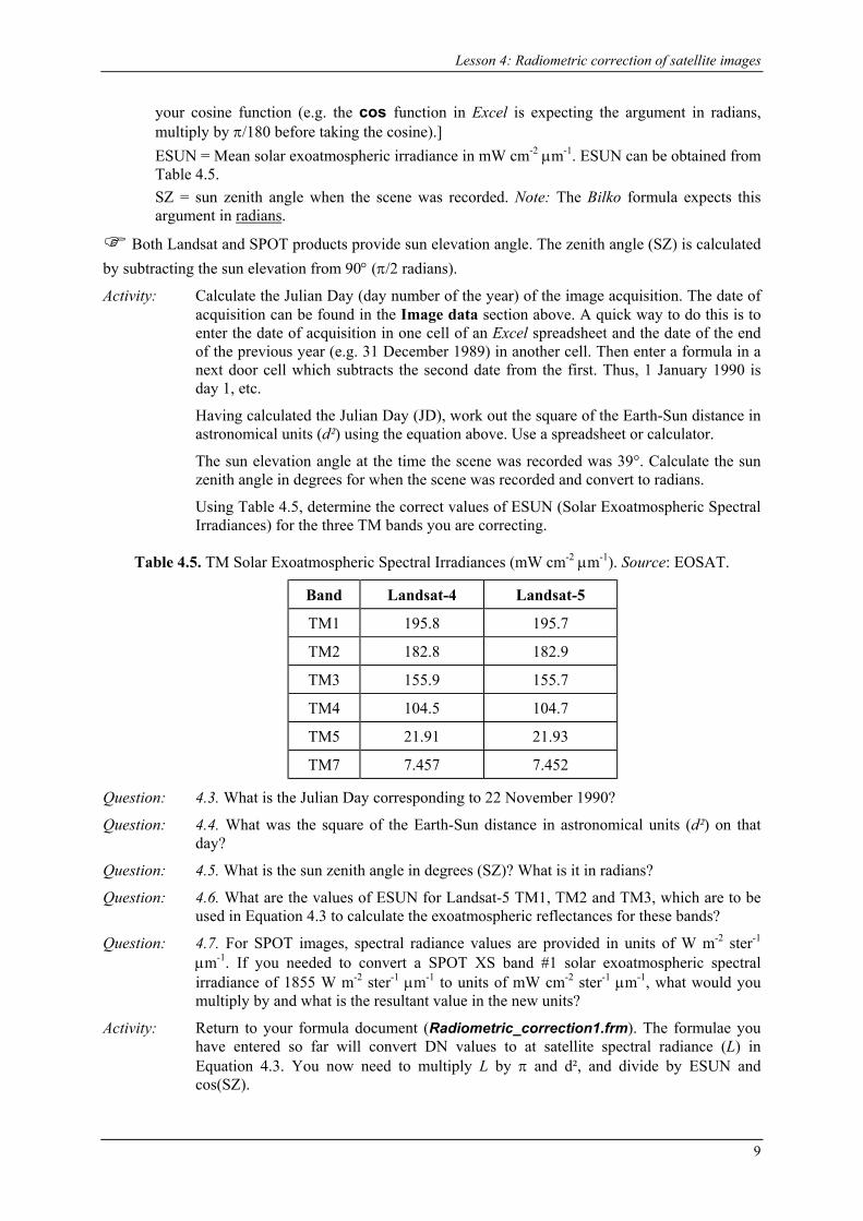
Using Table 4.5, determine the correct values of ESUN (Solar Exoatmospheric Spectral Irradiances) for the three TM bands you are correcting.
Table 4.5. TM Solar Exoatmospheric Spectral Irradiances (mW cm-2 µm-1). Source: EOSAT.
Band Landsat-4 Landsat-5
TM1 195.8 195.7
TM2 182.8 182.9
TM3 155.9 155.7
TM4 104.5 104.7
TM5 21.91 21.93
TM7 7.457 7.452
Question: 4.3. What is the Julian Day corresponding to 22 November 1990?
Question: 4.4. What was the square of the Earth-Sun distance in astronomical units (d²) on that day?
Question: 4.5. What is the sun zenith angle in degrees (SZ)? What is it in radians?
Question: 4.6. What are the values of ESUN for Landsat-5 TM1, TM2 and TM3, which are to be used in Equation 4.3 to calculate the exoatmospheric reflectances for these bands?
Question: 4.7. For SPOT images, spectral radiance values are provided in units of W m-2 ster-1 µm-1. If you needed to convert a SPOT XS band #1 solar exoatmospheric spectral irradiance of 1855 W m-2 ster-1 µm-1 to units of mW cm-2 ster-1 µm-1, what would you multiply by and what is the resultant value in the new units?
Activity: Return to your formula document (Radiometric_correction1.frm). The formulae you have entered so far will convert DN values to at satellite spectral radiance (L) in Equation 4.3. You now need to multiply L by π and d², and divide by ESUN and cos(SZ).
9

Applications of satellite and airborne image data to coastal management
Thus you need to substitute the formulae you have already entered for L in the equation.
[Hint: Enter details of what you are about to do as comments, after the formulae already entered. Also set up the new input values as constants. For example, the following might be appropriate:
# Step 2. Converting at satellite spectral radiance (L) to exoatmospheric reflectance # # Input values # ========== # pi = 3.141593 # d² = ?.?????? astronomical units. # SZ = ?.????? radians # ESUN: TM1 = ???.?, TM2 = ???.?, TM3 = ???.? # const pi =3.141593 ; const dsquared = ?.?????? ; const SZ = ?.????? ; const ESUN1 = ???.? ; const ESUN2 = ???.?; const ESUN3 = ???.? ; # Let at satellite spectral radiance = L # # Converting L to exoatmospheric reflectance with formulae of the type: # # pi * L * dsquared / (ESUN * cos(SZ)) ; ] Enter your formula here (see below)
Note that you can enter several constant statements on one line.
Activity: Once the constants and comments are entered, use Copy and Paste to copy the intermediate formulae you created earlier, down to beneath this information before commenting the originals out (inserting a # before them). [If you get an Error in formula message, check for errors. If it recurs just retype the formulae.] Put brackets around the copied formulae (but leave the ; outside!) and then add in the relevant values and mathematical operators to carry out Step 2 of the radiometric correction according to Equation 4.3.
When you have completed the formula document, you should have all lines as comments apart from the statements setting up the constants and the three lines of the final formulae, which will probably look horrendous. Each formula should have a total of four opening brackets and four closing brackets if written in the format suggested above.
Activity: Save the Formula document. Because the exoatmospheric reflectance ρ has a value between 0 and 1, the output image will need to be a floating point (32-bit image). So before applying your formula to the connected images you need to select Options! from the Bilko menu. In the Formula Options dialog box select 32-bit Floating point from the Output Image Type: drop-down menu. (You do not want any special handling of nulls.)
Question: 4.8. What would happen if the output image were an 8-bit integer image like the input Landsat TM images?
Activity: Apply the Formula document to the connected images using Copy and Paste. It will apply the formula with @1 in it to the TM band #1 image of DN values, the formula with @2 in it to the TM band #2 image, etc. [If you get an Error in formula message, check for errors.] The three resultant images will show exoatmospheric reflectance on a scale of 0–1.
10
Lesson 4: Radiometric correction of satellite images
Close the connected images window and original images (LandsatTM_Nov_DN#01.gif, LandsatTM_Nov_DN#02.gif and LandsatTM_Nov_DN #03.gif) as these are no longer required. Close the formula document.
Connect the three resultant (exoatmospheric reflectance) images as a stack. (The image derived from the TM band #1 image will be the @1 image, that from TM band #2 the @2 image, etc.)
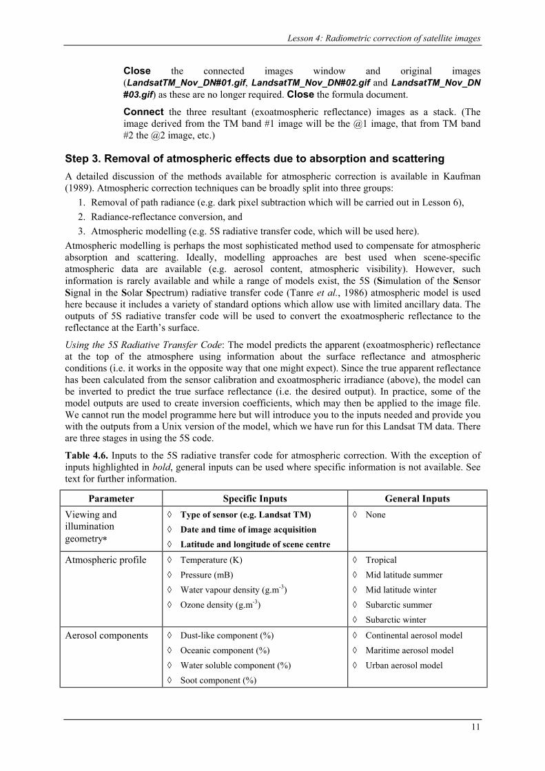
Step 3. Removal of atmospheric effects due to absorption and scattering A detailed discussion of the methods available for atmospheric correction is available in Kaufman (1989). Atmospheric correction techniques can be broadly split into three groups:
1. Removal of path radiance (e.g. dark pixel subtraction which will be carried out in Lesson 6), 2. Radiance-reflectance conversion, and 3. Atmospheric modelling (e.g. 5S radiative transfer code, which will be used here).
Atmospheric modelling is perhaps the most sophisticated method used to compensate for atmospheric absorption and scattering. Ideally, modelling approaches are best used when scene-specific atmospheric data are available (e.g. aerosol content, atmospheric visibility). However, such information is rarely available and while a range of models exist, the 5S (Simulation of the Sensor Signal in the Solar Spectrum) radiative transfer code (Tanre et al., 1986) atmospheric model is used here because it includes a variety of standard options which allow use with limited ancillary data. The outputs of 5S radiative transfer code will be used to convert the exoatmospheric reflectance to the reflectance at the Earth’s surface.
Using the 5S Radiative Transfer Code: The model predicts the apparent (exoatmospheric) reflectance at the top of the atmosphere using information about the surface reflectance and atmospheric conditions (i.e. it works in the opposite way that one might expect). Since the true apparent reflectance has been calculated from the sensor calibration and exoatmospheric irradiance (above), the model can be inverted to predict the true surface reflectance (i.e. the desired output). In practice, some of the model outputs are used to create inversion coefficients, which may then be applied to the image file. We cannot run the model programme here but will introduce you to the inputs needed and provide you with the outputs from a Unix version of the model, which we have run for this Landsat TM data. There are three stages in using the 5S code.
Table 4.6. Inputs to the 5S radiative transfer code for atmospheric correction. With the exception of inputs highlighted in bold, general inputs can be used where specific information is not available. See text for further information.
Parameter Specific Inputs General Inputs Viewing and illumination geometry∗
◊ Type of sensor (e.g. Landsat TM) ◊ Date and time of image acquisition ◊ Latitude and longitude of scene centre
◊ None
Atmospheric profile ◊ Temperature (K) ◊ Pressure (mB) ◊ Water vapour density (g.m-3) ◊ Ozone density (g.m-3)
◊ Tropical ◊ Mid latitude summer ◊ Mid latitude winter ◊ Subarctic summer ◊ Subarctic winter
Aerosol components ◊ Dust-like component (%) ◊ Oceanic component (%) ◊ Water soluble component (%) ◊ Soot component (%)
◊ Continental aerosol model ◊ Maritime aerosol model ◊ Urban aerosol model
11

Applications of satellite and airborne image data to coastal management
Aerosol concentration ◊ Aerosol optical depth at 550 nm ◊ Meteorological visibility (km)
Spectral band ◊ Lower and upper range of band (µm) ◊ Band name (e.g. Landsat TM3)
Ground reflectance (a) Choose homo- or heterogeneous surface (b) If heterogeneous, enter reflectance of target surface, surrounding surface and target radius (km)
As specific inputs except 5S supplies mean spectral value for green vegetation, clear water, sand, lake water
* this information is available in image header file and/or accompanying literature
Stage 1 - Run the 5S code for each band in the imagery
The inputs of the model are summarised in Table 4.6. Note that it is possible to input either a general model for the type of atmospheric conditions or, if known, specific values for atmospheric properties at the time the image was taken. In the event that no atmospheric information is available, the only parameter that needs to be estimated is the horizontal visibility in kilometres (meteorological range) which for our November image was estimated at 35 km (a value appropriate for the humid tropics in clear weather), but for the June image was significantly poorer at only 20 km.
Activity: Make a note of the following specific inputs needed to run the 5S code in Table 4.7. below:
Table 4.7. Specific inputs needed to run the 5S code for the two images.
Specific inputs November image June image
Type of sensor
Date and time of image acquisition
Latitude and longitude of scene centre
Meteorological visibility (km)
Stage 2 - Calculate the inversion coefficients and spherical albedo from the 5S code output
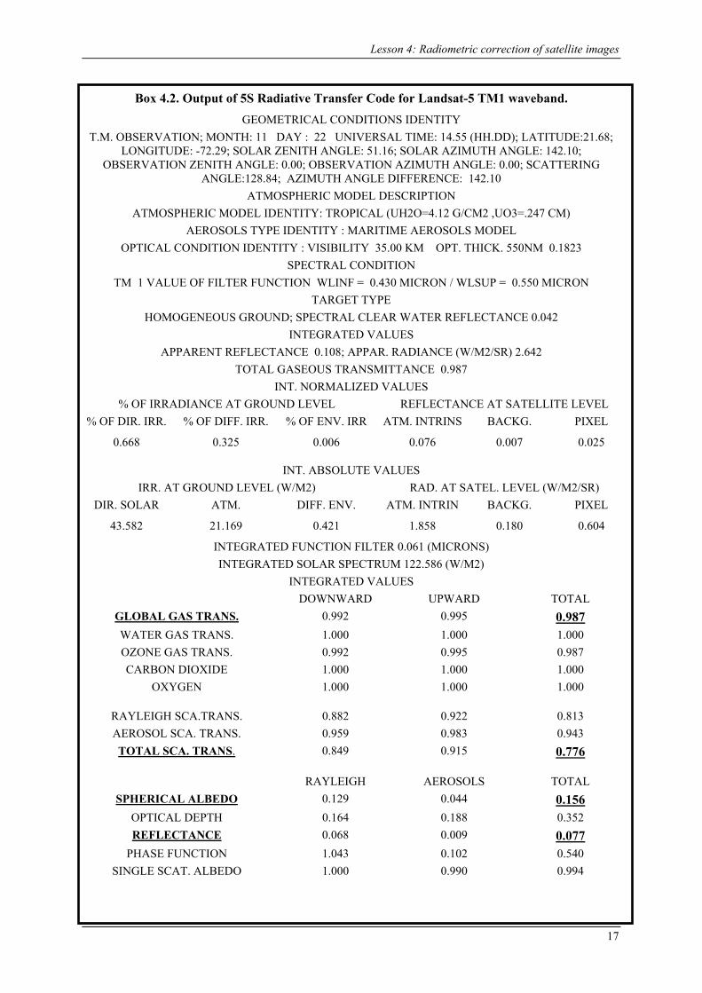
The 5S code provides a complex output but only some of the information is required by the user. The following example of the output for Landsat TM1 (Box 4.2) highlights the important information in bold.
Activity: Refer to Box 4.2 (see end of lesson) for Landsat TM1 values of key parameters (underlined and in bold) output by 5S atmospheric model and insert the global gas transmittance, total scattering transmittance, reflectance and spherical albedo values in Table 4.8 below. The values for bands TM2 and TM3 have already been entered from runs of the 5S radiative transfer code for these wavebands.
12

Lesson 4: Radiometric correction of satellite images
Table 4.8. Outputs from the 5S radiative transfer code and parameters calculated from these.
Parameter TM1 TM2 TM3
Global gas transmittance 0.917 0.930
Total scattering transmittance 0.854 0.897
Reflectance 0.044 0.027
Spherical albedo 0.108 0.079
AI (see Equation 4.4)
BI (see Equation 4.5)
Activity: Use these values and Equations 4.4 and 4.5 below to calculate the inversion coefficients AI and BI for each waveband and then enter these values (to 4 decimal places) in Table 4.8. This can be done on a spreadsheet or using a calculator.
AGlobal gas transmittance Total scattering transmittanceI =
×1 Equation 4.4
B ReflectanceTotal scattering transmittanceI =
− Equation 4.5
The coefficients AI and BI and the exoatmospheric reflectance data derived in Step 2 can then be combined using Formula documents to create new images Y for each waveband using Equation 4.6. [Note the minus sign in front of the Reflectance value in Equation 4.5, which means that BI will always be negative.]
Equation 4.6 ( )Y = A Exoatmospheric reflectance [ ] BI I× +ρ
where ρ are the values (exoatmospheric reflectances) stored in your new connected stacked images (@1, @2 and @3).
You now have the information needed to carry out Stages 2 and 3 of the atmospheric correction, which will convert your exoatmospheric reflectances to at surface reflectances. It is best to carry this out as two stages with intermediate formulae to create the new images Y for each waveband (Equation 4.6) and final formulae, incorporating these, to carry out Equation 4.7.
Activity: Open a new formula document and enter an appropriate header (modelled on what you did earlier) to explain what is being done and set up a series of constant statements for the new input data. Suggested constant names are AI1, AI2 and AI3 and BI1, BI2 and BI3 for the inversion coefficients.
For each waveband, create an intermediate formula to carry out Equation 4.6 of the type:
AI * @n + BI ;
where n = the waveband. Save the Formula document as Radiometric_ correction2.frm.
Stage 3 - Implementation of model inversion to the Landsat TM satellite imagery
Once you have set up the formulae to create the new images (Y) for each waveband using Equation 4.6, you can take the appropriate spherical albedo (S) values from Table 4.8 and use the following equation to obtain surface reflectance ρs on a scale of 0–1:
13
Applications of satellite and airborne image data to coastal management
ρ sY
1 SY=
+ Equation 4.7
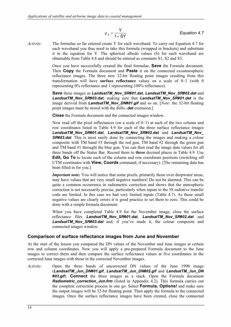
Activity: The formulae so far entered create Y for each waveband. To carry out Equation 4.7 for each waveband you thus need to take this formula (wrapped in brackets) and substitute it in the equation for Y. The spherical albedo values (S) for each waveband are obtainable from Table 4.8 and should be entered as constants S1, S2 and S3.
Once you have successfully created the final formulae, Save the Formula document. Then Copy the Formula document and Paste it on the connected exoatmospheric reflectance images. The three new 32-bit floating point images resulting from this transformation will have surface reflectance values on a scale of 0–1 (with 0 representing 0% reflectance and 1 representing 100% reflectance).
Save these images as LandsatTM_Nov_SR#01.dat, LandsatTM_Nov_SR#02.dat and LandsatTM_Nov_SR#03.dat, making sure that LandsatTM_Nov_SR#01.dat is the image derived from LandsatTM_Nov_DN#01.gif and so on. [Note: the 32-bit floating point images must be stored with the Bilko .dat extension.]
Close the Formula document and the connected images window.
Now read off the pixel reflectances (on a scale of 0–1) at each of the two column and row coordinates listed in Table 4.9 for each of the three surface reflectance images LandsatTM_Nov_SR#01.dat, LandsatTM_Nov_SR#02.dat and LandsatTM_Nov_ SR#03.dat. This is most easily done by connecting the images and making a colour composite with TM band #3 through the red gun, TM band #2 through the green gun and TM band #1 throught the blue gun. You can then read the image data values for all three bands off the Status Bar. Record them to three decimal places in Table 4.9. Use Edit, Go To to locate each of the column and row coordinate positions (switching off UTM coortinates with View, Coords command, if necessary). [The remaining data has been filled in for you.]
Important note: You will notice that some pixels, primarily those over deepwater areas, may have values that are very small negative numbers! Do not be alarmed. This can be quite a common occurrence in radiometric correction and shows that the atmospheric correction is not necessarily precise, particularly when inputs to the 5S radiative transfer code are limited. In this case we had very limited inputs (Table 4.7). As these small negative values are clearly errors it is good practice to set them to zero. This could be done with a simple formula document.
When you have completed Table 4.9 for the November image, close the surface reflectance files LandsatTM_Nov_SR#01.dat, LandsatTM_Nov_SR#02.dat and LandsatTM_Nov_SR#03.dat and, if you’ve made it, the colour composite and connected images window.
Comparison of surface reflectance images from June and November At the start of the lesson you compared the DN values of the November and June images at certain row and column coordinates. Now you will apply a pre-prepared Formula document to the June images to correct them and then compare the surface reflectance values at five coordinates in the corrected June images with those in the corrected November images.
Activity: Open the three bands of uncorrected DN values of the June 1990 image (LandsatTM_Jun_DN#01.gif, LandsatTM_Jun_DN#02.gif and LandsatTM_Jun_DN #03.gif). Connect the three images as a stack. Open the Formula document Radiometric_correction_Jun.frm (listed in Appendix 4.2). This formula carries out the complete correction process in one go. Select Formula, Options! and make sure the output images will be 32-bit floating point. Then apply the formula to the connected images. Once the surface reflectance images have been created, close the connected
14
Lesson 4: Radiometric correction of satellite images
images window and close LandsatTM_Jun_DN#01.gif, LandsatTM_Jun_ DN#02.gif and LandsatTM_Jun_DN#03 .gif.
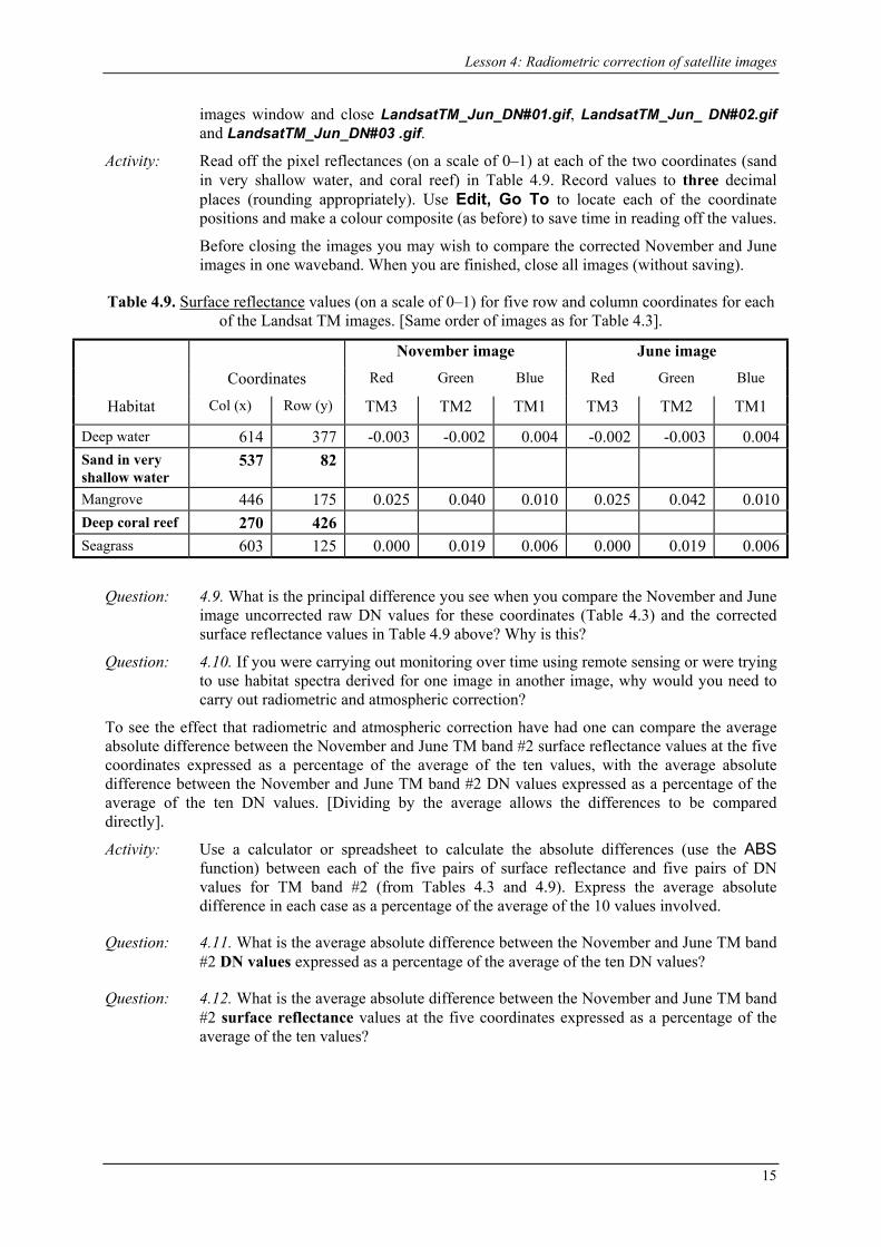
Activity: Read off the pixel reflectances (on a scale of 0–1) at each of the two coordinates (sand in very shallow water, and coral reef) in Table 4.9. Record values to three decimal places (rounding appropriately). Use Edit, Go To to locate each of the coordinate positions and make a colour composite (as before) to save time in reading off the values.
Before closing the images you may wish to compare the corrected November and June images in one waveband. When you are finished, close all images (without saving).
Table 4.9. Surface reflectance values (on a scale of 0–1) for five row and column coordinates for each of the Landsat TM images. [Same order of images as for Table 4.3].
November image June image
Coordinates Red Green Blue Red Green Blue
Habitat Col (x) Row (y) TM3 TM2 TM1 TM3 TM2 TM1
Deep water 614 377 -0.003 -0.002 0.004 -0.002 -0.003 0.004 Sand in very shallow water
537 82
Mangrove 446 175 0.025 0.040 0.010 0.025 0.042 0.010 Deep coral reef 270 426 Seagrass 603 125 0.000 0.019 0.006 0.000 0.019 0.006
Question: 4.9. What is the principal difference you see when you compare the November and June image uncorrected raw DN values for these coordinates (Table 4.3) and the corrected surface reflectance values in Table 4.9 above? Why is this?
Question: 4.10. If you were carrying out monitoring over time using remote sensing or were trying to use habitat spectra derived for one image in another image, why would you need to carry out radiometric and atmospheric correction?
To see the effect that radiometric and atmospheric correction have had one can compare the average absolute difference between the November and June TM band #2 surface reflectance values at the five coordinates expressed as a percentage of the average of the ten values, with the average absolute difference between the November and June TM band #2 DN values expressed as a percentage of the average of the ten DN values. [Dividing by the average allows the differences to be compared directly].
Activity: Use a calculator or spreadsheet to calculate the absolute differences (use the ABS function) between each of the five pairs of surface reflectance and five pairs of DN values for TM band #2 (from Tables 4.3 and 4.9). Express the average absolute difference in each case as a percentage of the average of the 10 values involved.
Question: 4.11. What is the average absolute difference between the November and June TM band #2 DN values expressed as a percentage of the average of the ten DN values?
Question: 4.12. What is the average absolute difference between the November and June TM band #2 surface reflectance values at the five coordinates expressed as a percentage of the average of the ten values?
15
Applications of satellite and airborne image data to coastal management
References Crippen, R.E. 1987. The regression intersection method of adjusting image data for band ratioing.
International Journal of Remote Sensing 8 (2): 137-155. Green, E.P., Mumby, P.J., Edwards, A.J. and Clark, C.D. (Ed. A.J. Edwards) (2000). Remote Sensing
Handbook for Tropical Coastal Management. Coastal Management Sourcebooks 3. UNESCO, Paris. ISBN 92-3-103736-6 (paperback).
Kaufman, Y.J. 1989. The atmospheric effect on remote sensing and its correction. In Asrar, G. (ed.) Theory and Applications of Optical Remote Sensing. John Wiley and Sons.
Moran, M.S., Jackson, R.D., Clarke, T.R., Qi, J. Cabot, F., Thome, K.J., and Markham, B.L. 1995. Reflectance factor retrieval from Landsat TM and SPOT HRV data for bright and dark targets. Remote Sensing of Environment 52: 218-230.
Potter, J.F., and Mendlowitz, M.A. 1975. On the determination of haze levels from Landsat data. Proceedings of the 10th International Symposium on Remote Sensing of Environment (Ann Arbor: Environmental Research Institute of Michigan). p. 695.
Price, J.C. 1987. Calibration of satellite radiometers and the comparison of vegetation indices. Remote Sensing of Environment 21: 15-27.
Switzer, P., Kowalik, W.S., and Lyon, R.J.P. 1981. Estimation of atmospheric path-radiance by the covariance matrix method. Photogrammetric Engineering and Remote Sensing 47 (10): 1469-1476.
Tanre, D., Deroo, C., Dahaut, P., Herman, M., and Morcrette, J.J. 1990. Description of a computer code to simulate the satellite signal in the solar spectrum: the 5S code. International Journal of Remote Sensing 11 (4): 659-668.
16
Lesson 4: Radiometric correction of satellite images
Box 4.2. Output of 5S Radiative Transfer Code for Landsat-5 TM1 waveband. GEOMETRICAL CONDITIONS IDENTITY
T.M. OBSERVATION; MONTH: 11 DAY : 22 UNIVERSAL TIME: 14.55 (HH.DD); LATITUDE:21.68; LONGITUDE: -72.29; SOLAR ZENITH ANGLE: 51.16; SOLAR AZIMUTH ANGLE: 142.10;
OBSERVATION ZENITH ANGLE: 0.00; OBSERVATION AZIMUTH ANGLE: 0.00; SCATTERING ANGLE:128.84; AZIMUTH ANGLE DIFFERENCE: 142.10
ATMOSPHERIC MODEL DESCRIPTION ATMOSPHERIC MODEL IDENTITY: TROPICAL (UH2O=4.12 G/CM2 ,UO3=.247 CM)
AEROSOLS TYPE IDENTITY : MARITIME AEROSOLS MODEL OPTICAL CONDITION IDENTITY : VISIBILITY 35.00 KM OPT. THICK. 550NM 0.1823
SPECTRAL CONDITION TM 1 VALUE OF FILTER FUNCTION WLINF = 0.430 MICRON / WLSUP = 0.550 MICRON
TARGET TYPE HOMOGENEOUS GROUND; SPECTRAL CLEAR WATER REFLECTANCE 0.042
INTEGRATED VALUES APPARENT REFLECTANCE 0.108; APPAR. RADIANCE (W/M2/SR) 2.642
TOTAL GASEOUS TRANSMITTANCE 0.987 INT. NORMALIZED VALUES
% OF IRRADIANCE AT GROUND LEVEL REFLECTANCE AT SATELLITE LEVEL % OF DIR. IRR. % OF DIFF. IRR. % OF ENV. IRR ATM. INTRINS BACKG. PIXEL
0.668 0.325 0.006 0.076 0.007 0.025
INT. ABSOLUTE VALUES IRR. AT GROUND LEVEL (W/M2) RAD. AT SATEL. LEVEL (W/M2/SR)
DIR. SOLAR ATM. DIFF. ENV. ATM. INTRIN BACKG. PIXEL
43.582 21.169 0.421 1.858 0.180 0.604
INTEGRATED FUNCTION FILTER 0.061 (MICRONS) INTEGRATED SOLAR SPECTRUM 122.586 (W/M2)
INTEGRATED VALUES
17
DOWNWARD UPWARD TOTAL GLOBAL GAS TRANS. 0.992 0.995 0.987 WATER GAS TRANS. 1.000 1.000 1.000 OZONE GAS TRANS. 0.992 0.995 0.987 CARBON DIOXIDE 1.000 1.000 1.000
OXYGEN 1.000 1.000 1.000
RAYLEIGH SCA.TRANS. 0.882 0.922 0.813 AEROSOL SCA. TRANS. 0.959 0.983 0.943 TOTAL SCA. TRANS. 0.849 0.915 0.776
RAYLEIGH AEROSOLS TOTAL
SPHERICAL ALBEDO 0.129 0.044 0.156 OPTICAL DEPTH 0.164 0.188 0.352 REFLECTANCE 0.068 0.009 0.077
PHASE FUNCTION 1.043 0.102 0.540 SINGLE SCAT. ALBEDO 1.000 0.990 0.994
Lesson 4: Radiometric correction of satellite images
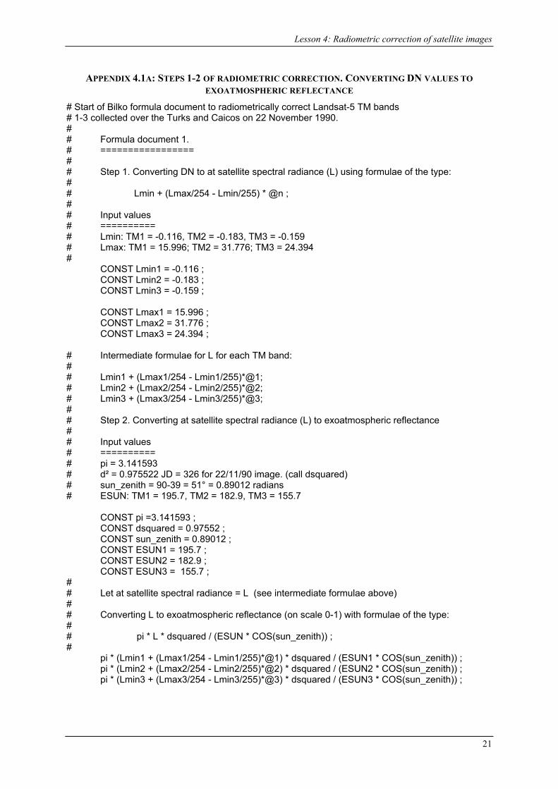
APPENDIX 4.1A: STEPS 1-2 OF RADIOMETRIC CORRECTION. CONVERTING DN VALUES TO EXOATMOSPHERIC REFLECTANCE
# Start of Bilko formula document to radiometrically correct Landsat-5 TM bands # 1-3 collected over the Turks and Caicos on 22 November 1990. # # Formula document 1. # ================= # # Step 1. Converting DN to at satellite spectral radiance (L) using formulae of the type: # # Lmin + (Lmax/254 - Lmin/255) * @n ; # # Input values # ========== # Lmin: TM1 = -0.116, TM2 = -0.183, TM3 = -0.159 # Lmax: TM1 = 15.996; TM2 = 31.776; TM3 = 24.394 # CONST Lmin1 = -0.116 ; CONST Lmin2 = -0.183 ; CONST Lmin3 = -0.159 ; CONST Lmax1 = 15.996 ; CONST Lmax2 = 31.776 ; CONST Lmax3 = 24.394 ; # Intermediate formulae for L for each TM band: # # Lmin1 + (Lmax1/254 - Lmin1/255)*@1; # Lmin2 + (Lmax2/254 - Lmin2/255)*@2; # Lmin3 + (Lmax3/254 - Lmin3/255)*@3; # # Step 2. Converting at satellite spectral radiance (L) to exoatmospheric reflectance # # Input values # ========== # pi = 3.141593 # d² = 0.975522 JD = 326 for 22/11/90 image. (call dsquared) # sun_zenith = 90-39 = 51° = 0.89012 radians # ESUN: TM1 = 195.7, TM2 = 182.9, TM3 = 155.7 CONST pi =3.141593 ; CONST dsquared = 0.97552 ; CONST sun_zenith = 0.89012 ; CONST ESUN1 = 195.7 ; CONST ESUN2 = 182.9 ; CONST ESUN3 = 155.7 ; # # Let at satellite spectral radiance = L (see intermediate formulae above) # # Converting L to exoatmospheric reflectance (on scale 0-1) with formulae of the type: # # pi * L * dsquared / (ESUN * COS(sun_zenith)) ; # pi * (Lmin1 + (Lmax1/254 - Lmin1/255)*@1) * dsquared / (ESUN1 * COS(sun_zenith)) ; pi * (Lmin2 + (Lmax2/254 - Lmin2/255)*@2) * dsquared / (ESUN2 * COS(sun_zenith)) ; pi * (Lmin3 + (Lmax3/254 - Lmin3/255)*@3) * dsquared / (ESUN3 * COS(sun_zenith)) ;
21
Applications of satellite and airborne image data to coastal management
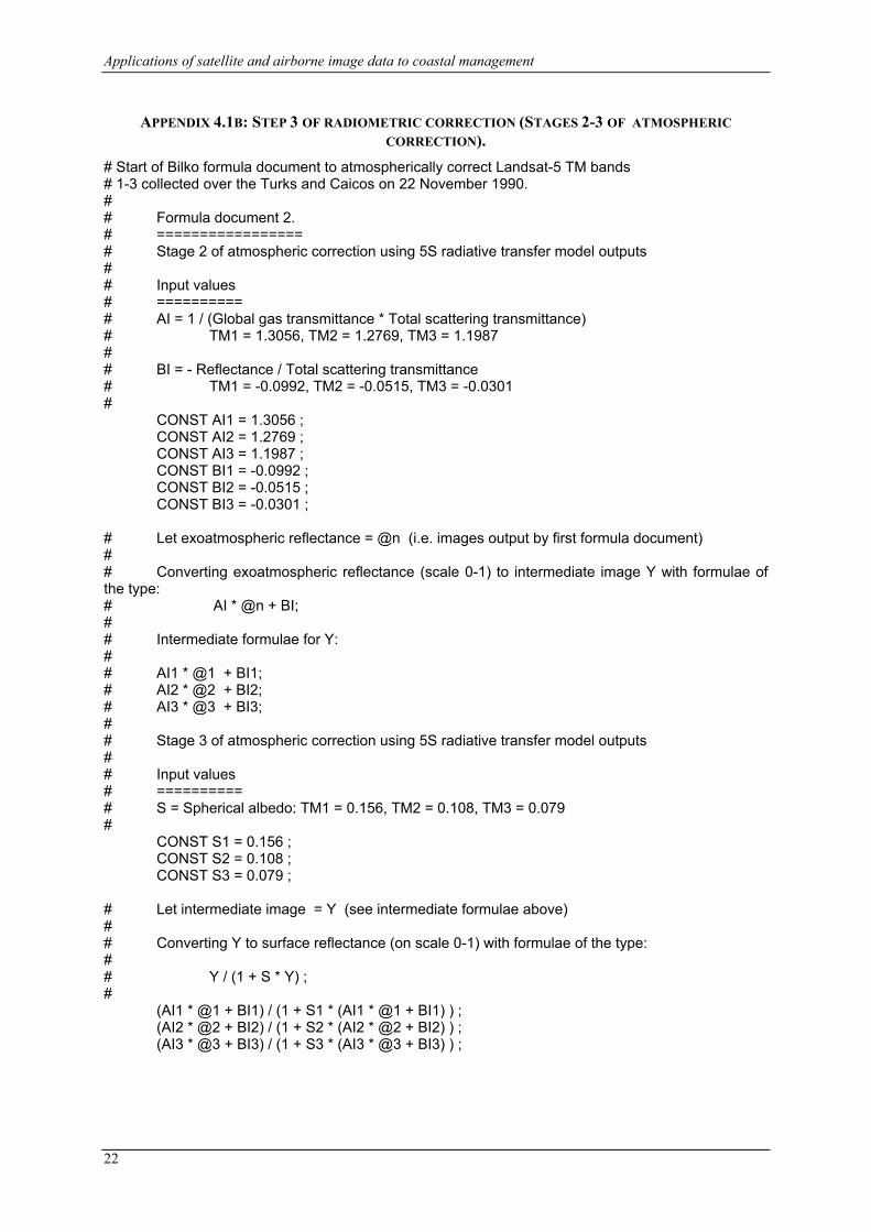
APPENDIX 4.1B: STEP 3 OF RADIOMETRIC CORRECTION (STAGES 2-3 OF ATMOSPHERIC CORRECTION).
# Start of Bilko formula document to atmospherically correct Landsat-5 TM bands # 1-3 collected over the Turks and Caicos on 22 November 1990. # # Formula document 2. # ================= # Stage 2 of atmospheric correction using 5S radiative transfer model outputs # # Input values # ========== # AI = 1 / (Global gas transmittance * Total scattering transmittance) # TM1 = 1.3056, TM2 = 1.2769, TM3 = 1.1987 # # BI = - Reflectance / Total scattering transmittance # TM1 = -0.0992, TM2 = -0.0515, TM3 = -0.0301 # CONST AI1 = 1.3056 ; CONST AI2 = 1.2769 ; CONST AI3 = 1.1987 ; CONST BI1 = -0.0992 ; CONST BI2 = -0.0515 ; CONST BI3 = -0.0301 ; # Let exoatmospheric reflectance = @n (i.e. images output by first formula document) # # Converting exoatmospheric reflectance (scale 0-1) to intermediate image Y with formulae of the type: # AI * @n + BI; # # Intermediate formulae for Y: # # AI1 * @1 + BI1; # AI2 * @2 + BI2; # AI3 * @3 + BI3; # # Stage 3 of atmospheric correction using 5S radiative transfer model outputs # # Input values # ========== # S = Spherical albedo: TM1 = 0.156, TM2 = 0.108, TM3 = 0.079 # CONST S1 = 0.156 ; CONST S2 = 0.108 ; CONST S3 = 0.079 ; # Let intermediate image = Y (see intermediate formulae above) # # Converting Y to surface reflectance (on scale 0-1) with formulae of the type: # # Y / (1 + S * Y) ; # (AI1 * @1 + BI1) / (1 + S1 * (AI1 * @1 + BI1) ) ; (AI2 * @2 + BI2) / (1 + S2 * (AI2 * @2 + BI2) ) ; (AI3 * @3 + BI3) / (1 + S3 * (AI3 * @3 + BI3) ) ;
22
Lesson 4: Radiometric correction of satellite images
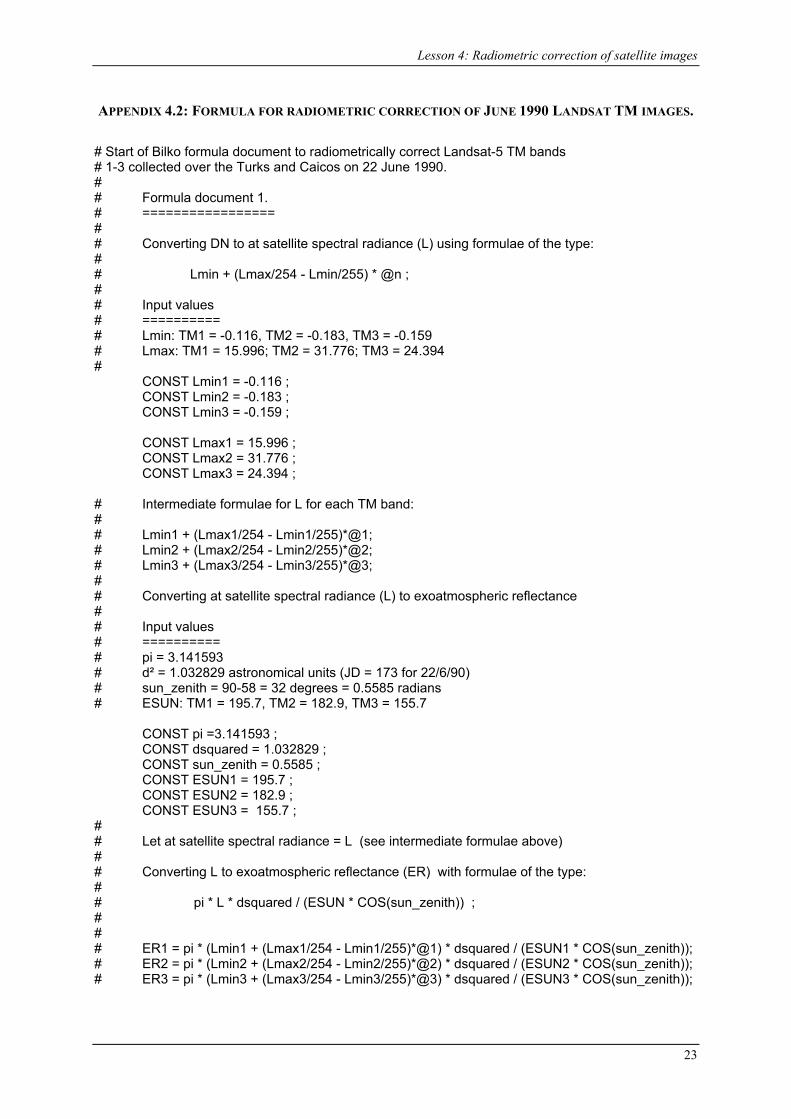
APPENDIX 4.2: FORMULA FOR RADIOMETRIC CORRECTION OF JUNE 1990 LANDSAT TM IMAGES.
# Start of Bilko formula document to radiometrically correct Landsat-5 TM bands # 1-3 collected over the Turks and Caicos on 22 June 1990. # # Formula document 1. # ================= # # Converting DN to at satellite spectral radiance (L) using formulae of the type: # # Lmin + (Lmax/254 - Lmin/255) * @n ; # # Input values # ========== # Lmin: TM1 = -0.116, TM2 = -0.183, TM3 = -0.159 # Lmax: TM1 = 15.996; TM2 = 31.776; TM3 = 24.394 # CONST Lmin1 = -0.116 ; CONST Lmin2 = -0.183 ; CONST Lmin3 = -0.159 ; CONST Lmax1 = 15.996 ; CONST Lmax2 = 31.776 ; CONST Lmax3 = 24.394 ; # Intermediate formulae for L for each TM band: # # Lmin1 + (Lmax1/254 - Lmin1/255)*@1; # Lmin2 + (Lmax2/254 - Lmin2/255)*@2; # Lmin3 + (Lmax3/254 - Lmin3/255)*@3; # # Converting at satellite spectral radiance (L) to exoatmospheric reflectance # # Input values # ========== # pi = 3.141593 # d² = 1.032829 astronomical units (JD = 173 for 22/6/90) # sun_zenith = 90-58 = 32 degrees = 0.5585 radians # ESUN: TM1 = 195.7, TM2 = 182.9, TM3 = 155.7 CONST pi =3.141593 ; CONST dsquared = 1.032829 ; CONST sun_zenith = 0.5585 ; CONST ESUN1 = 195.7 ; CONST ESUN2 = 182.9 ; CONST ESUN3 = 155.7 ; # # Let at satellite spectral radiance = L (see intermediate formulae above) # # Converting L to exoatmospheric reflectance (ER) with formulae of the type: # # pi * L * dsquared / (ESUN * COS(sun_zenith)) ; # # # ER1 = pi * (Lmin1 + (Lmax1/254 - Lmin1/255)*@1) * dsquared / (ESUN1 * COS(sun_zenith)); # ER2 = pi * (Lmin2 + (Lmax2/254 - Lmin2/255)*@2) * dsquared / (ESUN2 * COS(sun_zenith)); # ER3 = pi * (Lmin3 + (Lmax3/254 - Lmin3/255)*@3) * dsquared / (ESUN3 * COS(sun_zenith));
23
Applications of satellite and airborne image data to coastal management
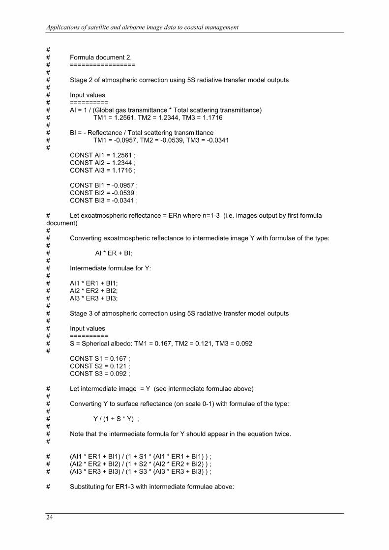
# # Formula document 2. # ================= # # Stage 2 of atmospheric correction using 5S radiative transfer model outputs # # Input values # ========== # AI = 1 / (Global gas transmittance * Total scattering transmittance) # TM1 = 1.2561, TM2 = 1.2344, TM3 = 1.1716 # # BI = - Reflectance / Total scattering transmittance # TM1 = -0.0957, TM2 = -0.0539, TM3 = -0.0341 # CONST AI1 = 1.2561 ; CONST AI2 = 1.2344 ; CONST AI3 = 1.1716 ; CONST BI1 = -0.0957 ; CONST BI2 = -0.0539 ; CONST BI3 = -0.0341 ; # Let exoatmospheric reflectance = ERn where n=1-3 (i.e. images output by first formula document) # # Converting exoatmospheric reflectance to intermediate image Y with formulae of the type: # # AI * ER + BI; # # Intermediate formulae for Y: # # AI1 * ER1 + BI1; # AI2 * ER2 + BI2; # AI3 * ER3 + BI3; # # Stage 3 of atmospheric correction using 5S radiative transfer model outputs # # Input values # ========== # S = Spherical albedo: TM1 = 0.167, TM2 = 0.121, TM3 = 0.092 # CONST S1 = 0.167 ; CONST S2 = 0.121 ; CONST S3 = 0.092 ; # Let intermediate image = Y (see intermediate formulae above) # # Converting Y to surface reflectance (on scale 0-1) with formulae of the type: # # Y / (1 + S * Y) ; # # Note that the intermediate formula for Y should appear in the equation twice. # # (AI1 * ER1 + BI1) / (1 + S1 * (AI1 * ER1 + BI1) ) ; # (AI2 * ER2 + BI2) / (1 + S2 * (AI2 * ER2 + BI2) ) ; # (AI3 * ER3 + BI3) / (1 + S3 * (AI3 * ER3 + BI3) ) ; # Substituting for ER1-3 with intermediate formulae above:
24

Lesson 4: Radiometric correction of satellite images
(AI1 * (pi * (Lmin1 + (Lmax1/254 - Lmin1/255)*@1) * dsquared / (ESUN1 * COS(sun_zenith))) + BI1) / (1 + S1 * (AI1 * (pi * (Lmin1 + (Lmax1/254 - Lmin1/255)*@1) * dsquared / (ESUN1 * COS(sun_zenith))) + BI1)); (AI2 * (pi * (Lmin2 + (Lmax2/254 - Lmin2/255)*@2) * dsquared / (ESUN2 * COS(sun_zenith))) + BI2) / (1 + S2 * (AI2 * (pi * (Lmin2 + (Lmax2/254 - Lmin2/255)*@2) * dsquared / (ESUN2 * COS(sun_zenith))) + BI2)); (AI3 * (pi * (Lmin3 + (Lmax3/254 - Lmin3/255)*@3) * dsquared / (ESUN3 * COS(sun_zenith))) + BI3) / (1 + S3 * (AI3 * (pi * (Lmin3 + (Lmax3/254 - Lmin3/255)*@3) * dsquared / (ESUN3 * COS(sun_zenith))) + BI3));
25

Applications of satellite and airborne image data to coastal management
Intentionally blank
26