
AifiilArtificial NlN eural NkN etworks - wmich.eduelise/courses/cs6800/Mohamed...• Artificial...
73
Transcript of AifiilArtificial NlN eural NkN etworks - wmich.eduelise/courses/cs6800/Mohamed...• Artificial...
AgendaAgenda
– Natural Neural NetworksNatural Neural Networks
– Artificial Neural Networks
XOR Example– XOR Example
– Design Issues
Applications– Applications
– Conclusion
2
Artificial Neural Networks?
• A technique for solving problems by
Artificial Neural Networks?
• A technique for solving problems by constructing software that works like our brains!brains!
3

Artificial Neural Networks?Artificial Neural Networks?
• A technique for solving problems byA technique for solving problems by constructing software that works like our brains!brains!
B h d b i k?• But, how do our brains work?
4
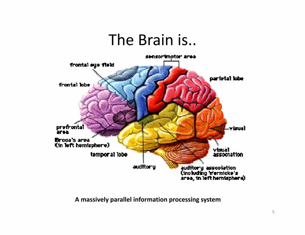
The Brain is..The Brain is..
5
A massively parallel information processing system

A HUGE network of processing lelements
6A typical brain contains a network of 10 billion neurons
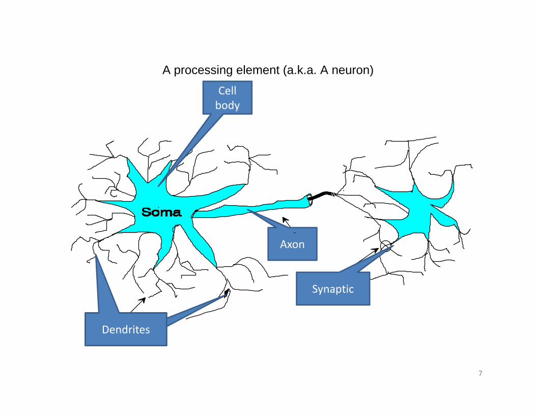
A processing element (a.k.a. A neuron)g ( )
Cell body
S y n a p s e
A x o n Axon
S i
D e n d r i te s
y p
Dendrites Dendrites
Synaptic
7
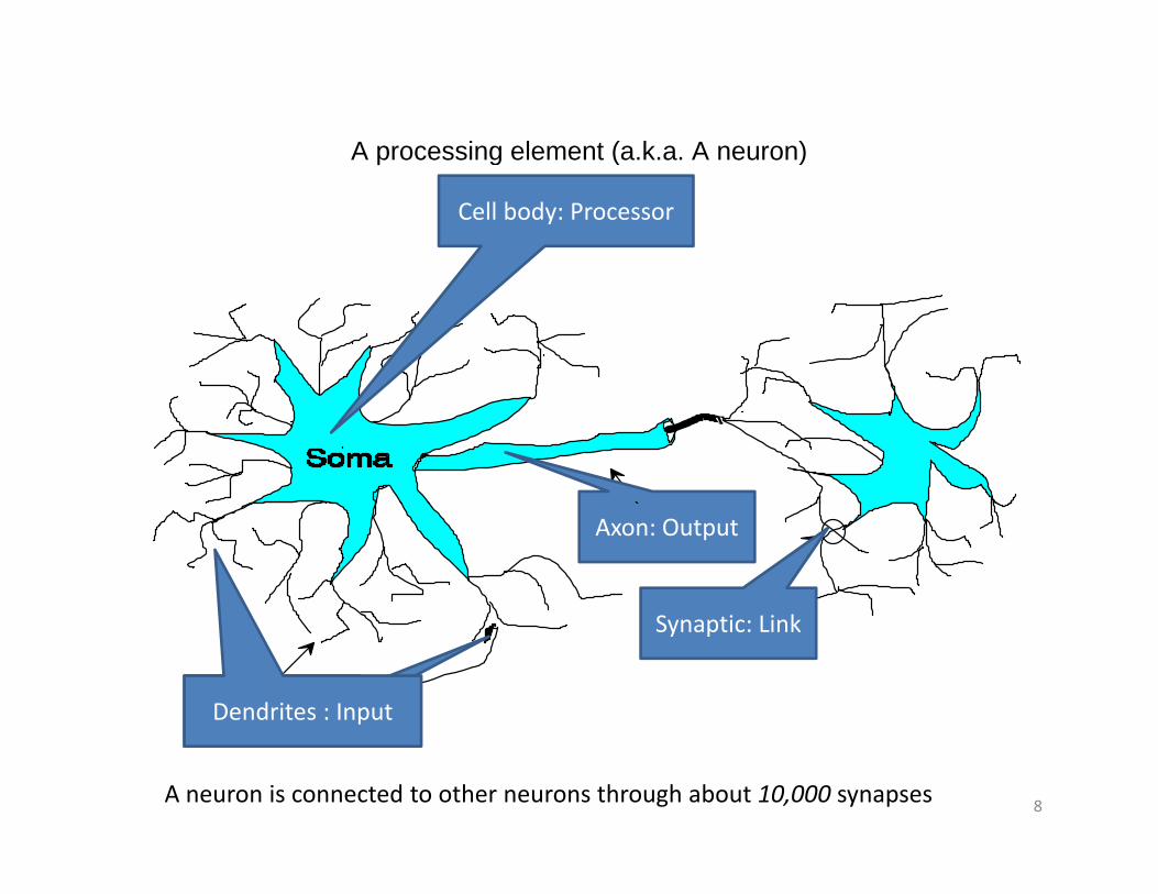
A processing element (a.k.a. A neuron)g ( )
Cell body: Processor
S y n a p s e
A x o n Axon: Output
S i Li k
D e n d r i te s
y p
Dendrites Dendrites : Input
Synaptic: Link
8A neuron is connected to other neurons through about 10,000 synapses
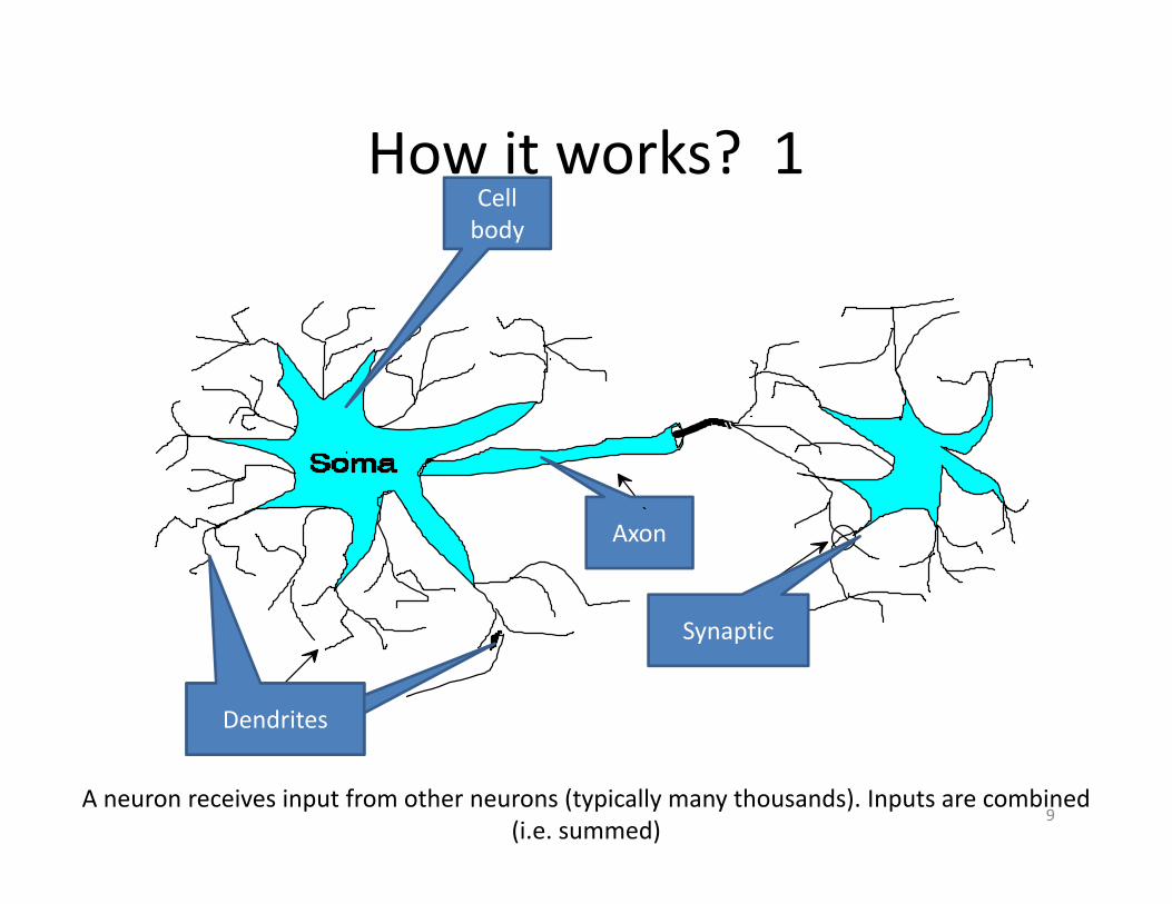
How it works? 1How it works? 1Cell body
S y n a p s e
A x o n Axon
S i
D e n d r i te s
y p
Dendrites Dendrites
Synaptic
9A neuron receives input from other neurons (typically many thousands). Inputs are combined
(i.e. summed)

How it works? 2How it works? 2Cell body
S y n a p s e
A x o n Axon
S i
D e n d r i te s
y p
Dendrites Dendrites
Synaptic
10Once input exceeds a critical level, the neuron discharges a spike ‐ an electrical pulse that travels
from the body, down the axon, to the next neuron(s)

How it works? 3How it works? 3Cell body
S y n a p s e
A x o n Axon
S i
D e n d r i te s
y p
Dendrites Dendrites
Synaptic
11The axon endings almost touch the dendrites or cell body of the next neuron

How it works? 3How it works? 3Cell body
S y n a p s e
A x o n Axon
S i
D e n d r i te s
y p
Dendrites Dendrites
Synaptic
12Transmission of an electrical signal from one neuron to the next is effected by neurotransmittors

How it works? 3How it works? 3Cell body
S y n a p s e
A x o n Axon
S i
D e n d r i te s
y p
Dendrites Dendrites
Synaptic
13Neurotransmittors are chemicals which are released from the first neuron and which bind to the
second

How it works? 4How it works? 4Cell body
S y n a p s e
A x o n Axon
S i
D e n d r i te s
y p
Dendrites Dendrites
Synaptic
14This link is called a synapse. The strength of the signal that reaches the next neuron depends on
factors such as the amount of neurotransmittor available

Neuron AbstractionNeuron Abstraction
15
So…So…
• An artificial network is an imitation of aAn artificial network is an imitation of a human neural network.
16

So…So…
• An artificial network is an imitation of aAn artificial network is an imitation of a human neural network.
• An artificial neuron is an imitation of a human neuron.
17
So…So…
• An artificial network is an imitation of aAn artificial network is an imitation of a human neural network.
• An artificial neuron is an imitation of a human neuron
• Let’s see an artificial neural network.
18

Cell BodyCell Body
19
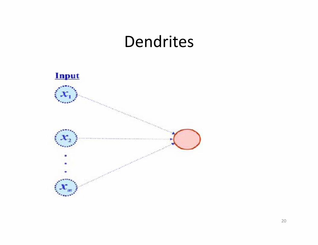
DendritesDendrites
20

Axon/SpikeAxon/Spike
21
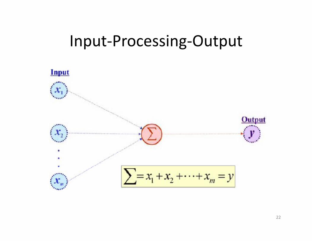
Input‐Processing‐OutputInput Processing Output
22

Not all inputs are equal!Not all inputs are equal!
23

Not all neurons are equal!Not all neurons are equal!
24

The signal is not passed down to the bnext neuron verbatim
Transfer Function
25

Three neuronsThree neurons
26

Input of a neuron=Output of other neuronsInput of a neuron Output of other neurons
27

Layer: A set of neurons that receive the same iinput
28

Three types of layers: Input, Hidden, and OutputThree types of layers: Input, Hidden, and Output
29
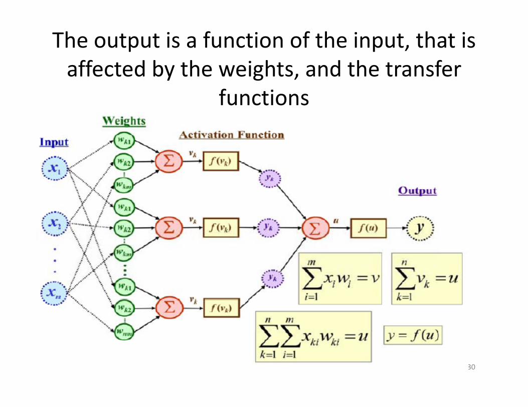
The output is a function of the input, that is affected by the weights, and the transferaffected by the weights, and the transfer
functions
30

A powerful tool…A powerful tool…
• An ANN can compute any computableAn ANN can compute any computable function, by the appropriate selection of the network topology and weights valuesnetwork topology and weights values.
31

A powerful tool…A powerful tool…
• An ANN can compute any computableAn ANN can compute any computable function, by the appropriate selection of the network topology and weights valuesnetwork topology and weights values.
Al ANN l f i !• Also, ANNs can learn from experience!
32

A powerful tool…A powerful tool…
• An ANN can compute any computableAn ANN can compute any computable function, by the appropriate selection of the network topology and weights valuesnetwork topology and weights values.
Al ANN l f i !• Also, ANNs can learn from experience!
• Specifically, by trial‐and‐error
33

Learning by trial‐and‐errorLearning by trial and error
• Continuous process of:Continuous process of:– Trial
Evaluate– Evaluate
– Adjust

Learning by trial‐and‐errorLearning by trial and error
• Continuous process of:Continuous process of:– Processing an input to produce an output (i.e. trial)
Evaluating this output (i e comparing it to the– Evaluating this output (i.e. comparing it to the expected output)
– Adjusting the “processing” “accordingly”– Adjusting the processing , accordingly
• In terms of ANN:C t th t t f ti f i i t– Compute the output function of a given input.
– Compare the actual output with the expected one
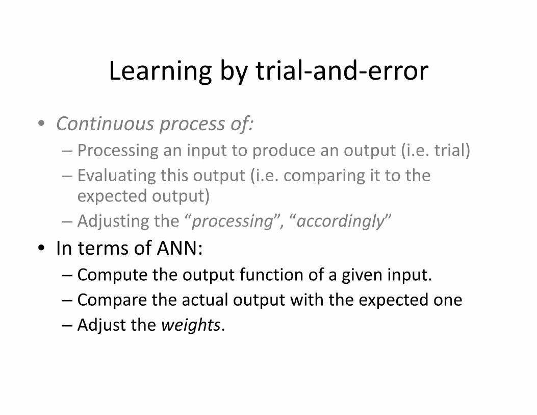
Learning by trial‐and‐errorLearning by trial and error
• Continuous process of:Continuous process of:– Processing an input to produce an output (i.e. trial)– Evaluating this output (i.e. comparing it to the g p ( p gexpected output)
– Adjusting the “processing”, “accordingly”
• In terms of ANN:– Compute the output function of a given input.– Compare the actual output with the expected one– Adjust the weights.
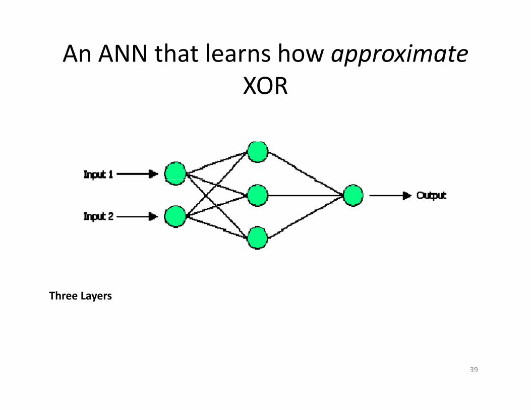
An ANN that learns how approximateXOR
Three Layers
39

An ANN that learns how approximateXOR
Input
Three Layers:Layer 1: Input Layer, with two neurons
40

An ANN that learns how approximateXORHidden
Three Layers:Layer 1: Input Layer, with two neuronsLayer 2: Hidden Layer, with three neurons
41
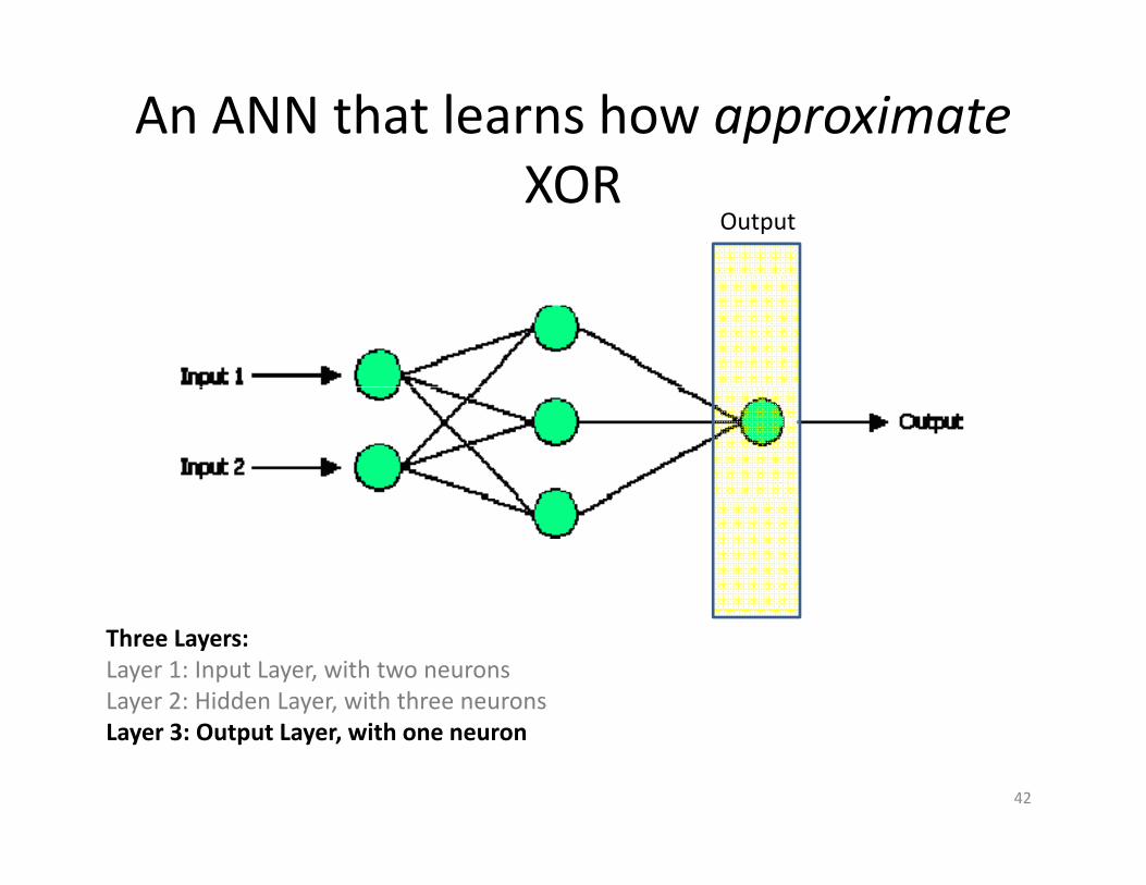
An ANN that learns how approximateXOR
Output
Three Layers:Layer 1: Input Layer, with two neuronsLayer 2: Hidden Layer, with three neurons
42
Layer 3: Output Layer, with one neuron
How it works?How it works?
• Set initial values of the weights randomlySet initial values of the weights randomly.
• Input: truth table of the XOR.
43

How it works?How it works?
• Set initial values of the weights randomlySet initial values of the weights randomly.
• Input: truth table of the XOR
• Do– Read input (e.g. 0, and 0)
44
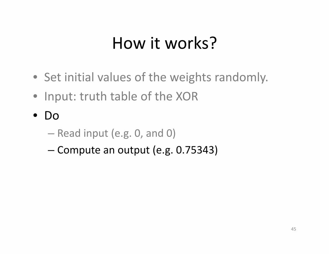
How it works?How it works?
• Set initial values of the weights randomlySet initial values of the weights randomly.
• Input: truth table of the XOR
• Do– Read input (e.g. 0, and 0)
– Compute an output (e.g. 0.75343)
45

How it works?How it works?
• Set initial values of the weights randomly.Set initial values of the weights randomly.• Input: truth table of the XOR• Do• Do
– Read input (e.g. 0, and 0)– Compute an output (e g 0 75343)– Compute an output (e.g. 0.75343)– Compute the error (the distance between the desired output and the actual output. (Error= p p (0.75343)
– Adjust the weights accordingly.
46

How it works?How it works?
• Set initial values of the weights randomly.• Input: truth table of the XOR• Do
R d i t ( 0 d 0)– Read input (e.g. 0, and 0)– Compute an output (e.g. 0.75343)– Compare it to the expected (i.e. desired) output. (Diff=
)0.75343)– Modify the weights accordingly.
• Loop until a condition is metp– Condition: certain number of iterations– Condition: error threshold
47

JOONEJOONE
48
Design IssuesDesign Issues
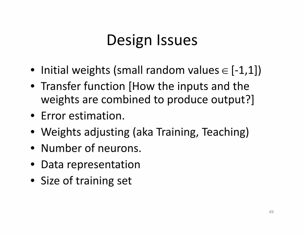
• Initial weights (small random values ∈[‐1,1])Initial weights (small random values ∈[ 1,1])• Transfer function [How the inputs and the weights are combined to produce output?]weights are combined to produce output?]
• Error estimation.• Weights adjusting (aka Training Teaching)• Weights adjusting (aka Training, Teaching)• Number of neurons.D t t ti• Data representation
• Size of training set
49

Transfer FunctionsTransfer Functions• Linear: The output is proportional to the total weighted input.g p
– Y=B*x, Y=B+x
• Threshold: The output is set at one of two values,Threshold: The output is set at one of two values, depending on whether the total weighted input is greater than or less than some threshold value.
• Non‐linear: The output varies continuously but not linearly as the input changes.
– Y= [Sigmoidal]2
2
2 ax
e−
50

Error EstimationError Estimation
• RMSE (Root Mean Square Error) is commonlyRMSE (Root Mean Square Error) is commonly used, or a variation of it.
– D(Yactual, Ydesired)=22 )()( actualdesired YY −
51

Weights AdjustingWeights Adjusting
• After each iteration weights should beAfter each iteration, weights should be adjusted to minimize the error.– All possible weights– All possible weights
– Hebbian learning
Artificial evolution– Artificial evolution
– Back propagation
52

Back PropagationBack Propagation
• N is a neuronN is a neuron.
• Nw is one of N’s inputs weights
• N is N’s output• Nout is N s output.
• Nw=Nw+ΔNw
• ΔNw =Nout* (1‐Nout)* NErrorFactor
• NErrorFactor=NExpectedOutput – NActualOutput
• This works only for the last layer, as we can know the actual output, and the expected output.
• What about the hidden layer?53
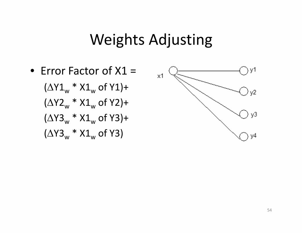
Weights AdjustingWeights Adjusting
• Error Factor of X1 =Error Factor of X1 = (ΔY1w * X1w of Y1)+(ΔY2 * X1 of Y2)+(ΔY2w * X1w of Y2)+(ΔY3w * X1w of Y3)+(ΔY3 * X1 f Y3)(ΔY3w * X1w of Y3)
54

Number of neuronsNumber of neurons
• Many neurons:– Higher accuracy – Slower– Risk of over‐fittingRisk of over fitting
• Memorizing, rather than understanding• The network will be useless with new problems.
• Few neurons:• Few neurons:– Lower accuracy– Inability to learn at all
• Optimal number:– Trail and error!– Adaptive techniques.Adaptive techniques.
55

Data representationData representation
• Usually input/output data needs pre‐processingUsua y put/output data eeds p e p ocess g• Pictures
– Pixel intensityy
• Smells– Molecule concentrations
• Text:– A pattern , e.g. 0‐0‐1 for “Chris”, 0‐1‐0 for “Becky”
• Numbers:– Decimal or binary
56

Size of training setSize of training set
• No one‐fits‐all formulaNo one fits all formula
• Some heuristics:Fi t t ti t i i l th b– Five to ten times training samples as the number of weights.
Greater thanW ||
– Greater than • |W|: number of weights
• a: desired accuracy
a−1
• a: desired accuracy
– Greater thannW log||
– Greater than • n: number of nodes
57
aa −− 1g
1
Applications AreasApplications Areas
• Function approximationFunction approximation
• Classification
Cl i• Clustering
• Pattern recognition (radar systems, face identification)
58

ApplicationsApplications
• Electronic NoseElectronic Nose
• NETtalk
59

Electronic NoseElectronic Nose
• Developed by Dr. Amy Ryan, at JPL, NASA.Developed by Dr. Amy Ryan, at JPL, NASA.• Goal: Detect low concentrations of dangerous gases.gases.– Ammonia is dangerous at a concentration of a few parts per million (ppm)
– Humans, can't sense it until it reaches about 50 ppm.
• An E‐Nose can differentiate between Pepsi, and Coca‐Cola. Can you?
60

Electronic NoseElectronic Nose
• An E‐Nose uses a collection of 16 differentAn E Nose uses a collection of 16 different polymer films.
• These films are specially designed to conductThese films are specially designed to conduct electricity.
• When a substance is absorbed into theseWhen a substance is absorbed into these films, the films expand slightly, and that changes how much electricity they conduct.
61
e- e- e- e- e- e-
Electronic NoseElectronic Nose
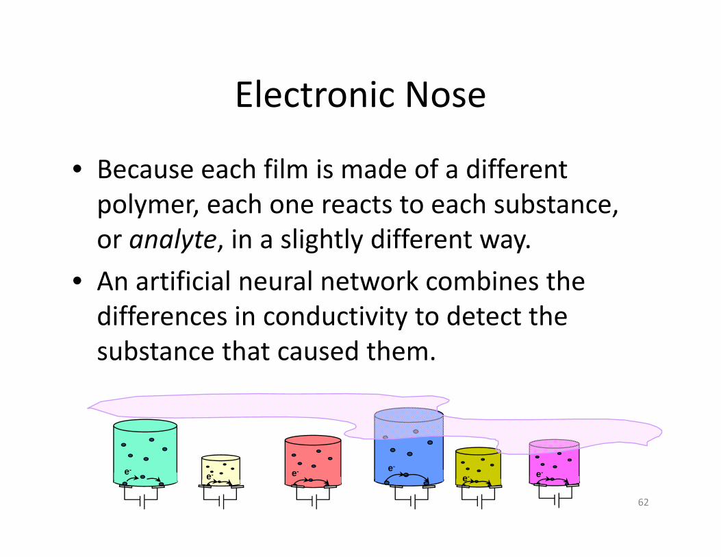
• Because each film is made of a differentBecause each film is made of a different polymer, each one reacts to each substance, or analyte in a slightly different wayor analyte, in a slightly different way.
• An artificial neural network combines the differences in conductivity to detect thedifferences in conductivity to detect the substance that caused them.
62
e- e- e-
e- e-e-

NETtalk ExperimentNETtalk Experiment
• Carried out in the mid 1980s by TerrenceCarried out in the mid 1980s by Terrence Sejnowski and Charles Rosenberg.
• Goal: teach a computer how to pronounce• Goal: teach a computer how to pronounce words.
Th k i f d d d h d• The network is fed words, and phonemes, and articulatory features.
• It really learns. Listen!
63

Advantages / DisadvantagesAdvantages / Disadvantages
• Advantagesg– Adapt to unknown situations– Powerful, it can model complex functions.– Ease of use, learns by example, and very little user domain‐specific expertise needed
• Disadvantages– ForgetsForgets– Not exact– Large complexity of the network structureLarge complexity of the network structure

Status of Neural NetworksStatus of Neural Networks
• Most of the reported applications are still• Most of the reported applications are still in research stage
• No formal proofs, but they seem to have useful applications that workuseful applications that work

ConclusionConclusion
• Artificial Neural Networks are an imitation of the t c a eu a et o s a e a tat o o t ebiological neural networks, but much simpler ones.
• ANNs can learn, via trial and error. • Many factors affect the performance of ANNs, such as the transfer functions, size of training sample, network topology, weights adjusting algorithmalgorithm, …
• No formal proofs, but they seem to have useful applicationsapplications.
66

RefrencesRefrences
• BrainNet II ‐ Creating A Neural Network Library• Electronic Nose • NETtalk, Wikipedia• A primer on Artificial Neural Networks, NeuriCam• Artificial Neural Networks Application, Peter Andras• Introduction to Artificial Neural Networks, Nicolas Galoppo von
Borries• Artificial Neural Networks, Torsten Reil• What is a "neural net"?• Introduction to Artificial Neural Network, Jianna J. Zhang,
B lli h AI R b i S i B lli h WABellingham AI Robotics Society, Bellingham WA• Elements of Artificial Neural Networks, Kishan Mehrotra, Chilukuri
K. Mohan and Sanjay Ranka, MIT Press, 1996
67Thanks to all folks who share there material online ☺

68

Learning ParadigmsLearning Paradigms
• Supervised learningSupervised learning
• Unsupervised learning
i f l i• Reinforcement learning
70

Supervised learningSupervised learning
• This is what we have seen so far!This is what we have seen so far!
• A network is fed with a set of training samples (inputs and corresponding output) and it uses(inputs and corresponding output), and it uses these samples to learn the general relationship between the inputs and therelationship between the inputs and the outputs.
Thi l i hi i d b h l• This relationship is represented by the values of the weights of the trained network.
71

Unsupervised learningUnsupervised learning
• No desired output is associated with theNo desired output is associated with the training data!
• Learning by doing!• Learning by doing!
• Faster than supervised learning
• Used to find out structures within data:– Clustering
– Compression
72

Reinforcement learningReinforcement learning
• Like supervised learning but:Like supervised learning, but:– Weights adjusting is not directly related to the error valueerror value.
– The error value is used to randomly, shuffle weights!weights!
– Slow, due to randomness.
73