Ahmed, Saʼad A. -Wahab (1989) Dynamic analyses of pile...

Glasgow Theses Service http://theses.gla.ac.uk/

[email protected]

Ahmed, Saʼad A. -Wahab (1989) Dynamic analyses of pile driving. PhD thesis. http://theses.gla.ac.uk/1123/ Copyright and moral rights for this thesis are retained by the author A copy can be downloaded for personal non-commercial research or study, without prior permission or charge This thesis cannot be reproduced or quoted extensively from without first obtaining permission in writing from the Author The content must not be changed in any way or sold commercially in any format or medium without the formal permission of the Author When referring to this work, full bibliographic details including the author, title, awarding institution and date of the thesis must be given

http://theses.gla.ac.uk/

DYNAMIC ANALYSES OF PILE DRIVING

BY

SA'AD A-W AHMED B. Sc. ; M. Sc. (CIVIL ENGG. )

A THESIS SUBMITTED FOR THE DEGREE OF DOCTOR OF PHILOSOPHY

DEPARTMENT OF CIVIL ENGINEERING

UNIVERSITY OF GLASGOW

SEPTEMBER - 1989

O SA'AD A-W AHMED

To my Wife Asjad and Sons Wakas and Wasak

ABSTRACT

Several approaches to the dynamic analyses of pile driving are explored in

this Thesis. These include pile driving formulae, single degree of freedom (SDOF)

models, the wave equation approach and a finite element model.

In the elementary models, the pile is modelled as a rigid mass while the soil

is represented by various simple rheological mechanisms (spring-slider-dashpot

models). Analytical and numerical formulations are developed and the parametric

results of the analyses are presented in non-dimensional form.

A study of the wave equation method of the analysis culminates in the

development of some simple analytical expressions (analogous to the pile driving

formulae) which may prove useful in practice. Some comparisons between the

elementary SDOF models, the pile driving formulae and the wave equation have

been undertaken in order to assess their strengths and highlight their various

shortcomings.

The development of a finite element model for pile driving is discussed in

detail with particular emphasis on spatial discretisation (especially the viscous

boundaries) and the time integration schemes. A limited parametric study has

been conducted in order to gain some insight into the behaviour of piles during

driving and to follow the evolution of failure in soils around and beneath the

piles. Further work in this area is indicated although computational costs seems to

be too high to justify routine use of the finite element method.

1

ACKNOWLEDGEMENTS

The work described in this Thesis was carried out at the Department of

Civil Engineering at Glasgow University under the direction of Dr. T. G. Davies.

I am greatly indebted to him for his invaluable advice and encouragement

throughout the work and for many suggestions for improvements to this Thesis.

My thanks are due to Dr. D. R. Green, the Head of the Department, for

allowing me the use of the facilities of the Department. I also wish to thank

Professor D. Muir Wood for his interest in this research study.

I am deeply grateful to Miss. J. Sutherland, for her invaluable help in the

enhancement of the Computer Program MIXDYN.

My thanks are also due to my wife for her support and encouragement

throughout my work.

I would also like to acknowledge the support of my fellow research students,

who were always willing to discuss aspects of my work with me.

Finally, my thanks are due to the Iraqi Embassy for their financial support,

without which the work could not have been completed.

S. A-W AHMED

11

CONTENTS

Page No.

ABSTRACT

ACKNOWLEDGEMENT

CONTENTS

NOTATION

CHAPTER

CHAPTER

CHAPTER

1 INTRODUCTION

1.1 INTRODUCTION

1.2 LITERATURE REVIEW

1.2.1 Pile Driving Formulae

1.2.2 Wave Equation Method

1.2.3 Finite Element Method

1.3 CLOSURE

2 ELEMENTARY MODELS

2.1 INTRODUCTION

2.2 PILE DRIVING FORMULAE

2.2.1 Introduction

2.2.2 Formulation

2.2.3 Discussion

2.3 SINCLE DECREE OF FREEDOM MODELS

2.3.1 1 nt roduct ion

2.3.2 Pile subjected to Initial Velocity

2.3.3 Results

2.3.4 Pile subjected to Cushioned Impact

2.3.5 Results

2.3.6 Discussion

2.4 CONCLUSION

3 THE WAVE EQUATION MODEL

3.1 INTRODUCTION

3.2 FORMULATION

3.2.1 Discrete Equations

3.2.2 Critical Time Step

3.3 NUMERICAL IMPLEMENTATION

1

11

111

vi

1-14

1

2

2

4

7

8

15 -70 15

15

15

16

19

19

19

20

26

28

30

31

32

71-159

71

72

72

74

75

111

Page No.

CHAPTER

CHAPTER

3.4 RESULTS 76

3.4.1 Wave Equation 76

3.4.2 Comparison with Elementary Models 79

3.4.2.1 Wave Equation versus SDOF Model 79

3.4.2.2 Wave Equation versus Pile Driving Formulae 81

3.5 DISCUSSION 85

3.6 CONCLUSION 85

4 THE FINITE ELEMENT MODEL 160 -218

4.1 INTRODUCTION 160

4.2 THEORETICAL FORMULATION 160

4.2.1 Introduction 160

4.2.2 Governing Equations 161

4.3 CONSTITUTIVE LAWS 169


4.3.2 Yield Criteria 170

4.3.3 The Critical State Model 173

4.3.4 Conclusion 177

4.4 SPATIAL DISCRETISATION 177


4.4.2 Geometric Modelling 178

4.4.3 Transmitting Boundaries 179

4.4.4 Interface Elements 186

4.5 TIME INTEGRATION SCHEMES 187


4.5.2 Explicit Integration Schemes 188

4.5.3 Implicit Integration Schemes 191

4.5.4 Implicit-Explicit Integration Schemes 193

4.5.5 Conclusion 194

4.6 CONCLUSION 194

5 FINITE ELEMENT ANALYSIS OF PILE DRIVING 219 -259 5.1 INTRODUCTION 219

5.2 CONVERGENCE STUDIES 220

5.3 PARAMETRIC STUDIES 221

5.4 DISCUSSION 224

1v

Page No.

5.5 CONCLUSION

CHAPTER 6 CONCLUSIONS AND RECOMMENDATIONS FOR

FUTURE STUDIES

6.1 CONCLUSIONS

6.2 RECOMMENDATIONS FOR FUTURE STUDIES

REFERENCES

APPENDIX A COMPUTER PROCRAM

APPENDIX B SUBROUTINE SDAMP

APPENDIX C PROCRAM WAVE

224

260 -261 260

261

262

275

284

286

V

NOTATION

Symbols which are not given below are defined in the text.

I Elementary Models and Wave Equation:

A cross sectional area of the pile

C ratio between the actual pile head displacement and that

given by Hooke's law

E Young-'s modulus of elasticity

EP Young's modulus of elasticity of the pile

E, energy reaching the pile

E2 energy left after impact

ef efficiency factor for the hammer

e9 efficiency factor for impact

9 gravitational acceleration

H drop height of the hammer

i viscous damping coefficient of soil

KP internal spring (pile) stiffness

Ks external spring (soil) stiffness

L pile length

m mass

mp pile mass

mr ram mass

n coefficient of restitution

n soil to pile stiffness ratio (Ks/K P) Q quake value

R ultimate soil resistance

S permanent pile penetration per blow (set)

AS pp plastic deformation of pile

ASep elastic deformation of pile

ASes elastic deformation of soil

t time

At time interval

T period (2rl/w)

u hammer velocity after impact

vi

uP pile velocity after impact

v hammer velocity before impact

vP pile velocity before impact

V velocity of discrete pile mass

VO initial velocity V dimensionless velocity (V. J)

W circular frequency f-(-K1m)

Wnt dimensionless time

W weight of the hammer

0 numerical coefficient

Soil and Foundation Parameters/Finite Element Model:

E Young's modulus of elasticity

C shear modulus of elasticity

p Poisson's ratio

P mass density

cu undrained cohesive strength of soil

a adhesion coefficient at pile-soil interface

ro radius of the pile

isli p damping coefficients for pile shaft, pile tip, respectively

Vs1V p shear and compression wave velocities, respectively

Stress and Strain Parameters:

0', 7' normal and shear stresses, respectively

E normal strain

I stress invariant

i deviator stress invariant

F yield function

vii

Matrices and Vectors:

C damping matrix

F force matrix

M mass matrix K stiffness matrix

c diagonal damping matrix f diagonal force matrix

m diagonal mass matrix k diagonal stiffness matrix

Dynamic Analysis Parameters:

000 x, x, x displacement, velocity and acceleration, respectively At time step

t time

c velocity of the stress wave

a'a Newmark collocation parameters

SyLnbols for Transmitting Boundaries:

fixed boundary

roller boundary

viscous boundary

viii

CHAPTER 1

INTRODUCTION

1.1 INTRODUCTION


1.2.1 Pile Driving Formulae

1.2.2 Wave Equation Method


1.3 CLOSURE

CHAPTER 1

INTRODUCTION

1.1 INTRODUCTION

Load tests provide the most reliable means of determining the bearing

capacities of piles but such tests are expensive and laborious to perform.

Consequently, the performance of piles during driving is usually used as an

indicator of their subsequent load capacities. This process of interpretation may be

effected by such means as the pile driving formulae (e. g. the Hiley Formula) or,

latterly, the wave equation method (incorporated into field equipment such as the

Pile Driving Analyser). Even more sophisticated are the Finite Element analyses,

but these remain as yet within the domain of research although some applications

to critical offshore installations have been reported in the literature. The major

thrust of this Thesis is a critical examination of these various approaches to the

analysis of pile driving and to extend the current knowledge of the mechanics of

the driving process.

Chapter Two begins with a brief review of pile driving formulae, their

reliability and accuracy. Some simple single degree of freedom (mass--spring-

dashpot) models of pile driving are then considered and the results of a

parametric study of the problem are discussed.

Chapter Three deals with the wave equation method of analysis (in which

the pile is idealised as a compressible body) and the results are then compared

with those predicted by the elementary models described in Chapter Two. These

comparisons culminate in a new "pile driving formula".

In Chapter Four, the finite element method and its applications to

non-linear dynamic analyses is discussed. The modelling of infinite boundaries, the

pile-soil interface (slip) conditions, yield criteria for soils and spatial and temporal

discretisations are discussed in detail.

1

Chapter Five documents the results of a limited parametric study of the pile

driving problem using the finite element model. Parameters examined in this study

include the soil strength, stiffness, pile-soil adhesion and the pile-head loading

conditions, and the evolution of failure in the soil around and underneath the pile

during driving is examined. Finally, in Chapter Six, the relevance of each of

these methods to engineering practice is discussed and some recommendations for

further research effort are proposed.


The literature on pile driving analyses is extensive and the subject commands

the attention of a long running series of international conferences. In this section,

a representative set of some of the more important publications is briefly

reviewed. Some publications which deal with narrow specialist topics, particularly

in the finite element domain, are reviewed in the relevant Chapters.

1.2.1 P-ile Driving Formulae

The most frequently used method of estimating the load carrying capacity of

driven piles is to use pile driving formulae, Taylor (1948). The basic principle of

these formulae is that the energy input from the hammer is dissipated in the pile

and surrounding soil. However, there are major differences between different pile driving formulae in the way in which they account for the various energy losses.

All these formulae relate the ultimate load capacity to the pile set and, in

practice, it is often assumed that the driving resistance is equal to the load

carrying capacity of the pile. Pile driving formulae can not predict the effect of

soil consolidation etc. subsequent to driving on pile bearing capacities.

Agerschou (1962) analysed statistically the Engineering News Record (ENR)

formula based on data from 171 load tests to failure of piles embedded in sands

and gravel. The piles were driven by drop hammers and single/double acting

2

steam hammers. He concluded that the ENR formula was unreliable because 96%

of the allowable loads determined from this formula would have safety factors

varying from 1.1 to 30. He also suggested that there was no way of knowing a

priori what the safety factor was. However, he found that the Hiley formula and

Janbu formula were much more accurate.

Flaate (1964) discussed the derivation of the general pile driving formula and

the limitations and use of three pile driving formulae, namely, the Hiley formula,

the Engineering News Record formula and the Janbu formula. Results from a

great number of loading tests on piles were analysed statistically. All the piles

were driven in a mainly cohesionless material or through a cohesive material into

a dense cohesionless layer; the bearing capacity of piles thus being obtained in a

cohesionless material. He found that the mean nominal safety factors of these

formulae (Hiley, ENR and Janbu) were 2.7,6.0 and 3.0, respectively. However,

the wide range of safety factors given by the ENR formula were so great that

Flaate advocated abandoning the formula. Both the Hiley formula and the Janbu

formula gave relatively good results, but of these two the Janbu was judged to be

preferable.

Housel (1966) analysed data drawn from research conducted by the Michigan

State Highway Department into the performance characteristics of pile driving

hammers and piles. Eighty-eight instrumented piles were driven at three sites

using several different pile driving hammers and load tests were conducted on

nineteen of these piles to determine their static bearing capacities. The pile

lengths tested varied from 13 rn to 54 m and their bearing capacities were

estimated using pile driving formulae. Housel concluded that the ENR formula

yielded safety factors ranging from about one to a maximum of three or four,

compared with its implicit safety factor of six.

Poulos and Davis (1980) discussed pile driving formulae in detail. They

concluded from their literature survey that the Janbu formula, Danish formula

and Hiley Formula were the most reliable while Engineering News Record (ENR)

formula was the least reliable.

3

1.2.2 Wave Eguation Method

The gradual realisation that pile driving cannot be accurately analysed by

ri id body mechanics (pile d 9 riving formulae) led to the development of an analysis 1 utilizing wave theory. This method of analysis takes into account the fact that

hammer blows produce stress waves that pro pagate along pile shafts. A wave

equation approach was first considered by Isaacs (1931) and Fox (1932) but Smith

(1955,1960) was the first to carry out numerical calculations by this method.

The wave equation method is based on consideration of the one-dimensional

dynamic equilibrium of a prismatic bar subjected to impact at one end. It can be

shown that the differential equation of motion is:

-a7-t22 = CZ ax2 (1.1>

where, the wave velocity c is defined as follows:

C=�(p) (1.2)

where,

E is the Young's modulus of elasticity of the bar,

p is the mass density,

u is the displacement on the bar from its original position, and,

t is the time.

In pile driving analyses, the resistance of the surrounding soil must also be

considered. Equation 1.1 then becomes:

a2u 2

a2u c at2 ax2

where R is the soil resistance.

(1.3)

4

Unfortunately, an analytic solution to this equation is not possible. Hence,

recourse is made to numerical solutions such as that developed by Smith (1955)

and (1960). In Smith's (1955) paper he solved the wave equation by means of a

simple numerical technique (essentially a multidegree of freedom analysis) in

preference to a direct finite difference approach. In this numerical solution, the

pile shaft was subdivided into so-called "unit lengths" (finite segments) connected

by springs. He showed however that the solution was not unconditionally stable

and, in particular, the time integration scheme failed if time intervals greater than

some critical value were employed. In his later paper (Smith, 1960), the soil

resistance along the shaft and below the pile tip was idealised by slider-spring

and dashpot mechanisms. The springs (soil) deform linearly elastically a certain distance (termed the quake, Q) then fail plastically at the ultimate resistance R.

The dashpots were characterised by their coefficients of viscous damping, J.

Hirsch et. al, (1970) studied the effect of various parameters (including type

and size of hammer and pile and soil conditions) on the bearing capacities

predicted by the wave equation method. They found that the driving accessories

significantly affected the pile driving performance and that stiffer piles could

overcome greater soil resistance to penetration. They recommended use of

cushions of low stiffness in order to facilitate energy transfer and to limit driving

stresses.

Poulos and Davis (1980) discussed Smith's (1960) empirical soil parameters;

quake, Q, and coefficient of viscous damping, J. They thought that it might be

possible to derive values of Q theoretically from pile-settlement theory and,

hence, quake values would vary along the pile shaft with the values near the pile

tip being greater than those along the shaft. They gave empirical correlations

between the coefficient of viscous damping for the pile tip JP and pile shaft Js

and soil type. Further, they suggested that the available data confirmed that pile

tip viscosity was several times greater than shaft viscosity, typically JP= 3JS, They

presented some results which showed that pile length above the ground and

embedded pile length had little effect on pile driving performance. They showed

that pile bearing capacities increased only slowly with increased hammer energy

and suggested that there would be an optimum cushion stiffness that could

provide protection for both the hammer and the pile while not seriously affecting

the driving capability of the system. They also showed that pile impedance had a

5

significant influence on peak driving stresses. Higher impedance piles (heavier

and/or stiffer sections) induced higher peak stresses than the lighter sections.

Authier and Fellenius (1980) presented the results of a comprehensive study

of quake values determined from dynamic measurements. In their analysis, they

use the Case Pile Driving Analysis Program (CAPWAP). Good results were

obtained for piles driven into a very dense sandy silty glacial till using tip quake

value of 20 mm rather than the usual value of 2.5* mm. However, for piles

driven through thick clay deposits into underlying dense clayey silty glacial tills,

good results were obtained with 8 mm quake values. The authors believed that

the large quakes observed might be related to pore pressure build-up in the soil.

The occurrence of large quakes has practical importance since they inhibit driving.

Ebecken et. al. (1984) described a numerical solution based on the

discretisation of piles into one-dimensional finite elements. The soil was

represented by non-4inear springs and dashpots attached to the finite elements at

their nodes. Their soil model allowed soil degradation during load cycles and they

applied the model to calcareous soils in Brazil.

Corte and LeDert (1986) proposed a new soil model to describe the soil

shaft resistance. In this model, the soil was separately idealised into two zones (Fig. 1.1a); the first zone of the model simulates the soil reacti on to large strains

while in the second (outer) zone the soil response is elastic. They showed that

this soil model could allow larger velocities in the pile than in the soil during

penetration and believed that this would give better estimates of energy radiated

by elastic waves than Smith's (1960) model.

Wu et. al, (1986) described a soil model (shown in Fig. 1.2b) consisting of

a slip mechanism and an elastic shear wave energy absorbing boundary. The

accuracy of the model was verified by comparing its predictions with those

obtained from a finite element analysis (Fig. 1.2a).

Yij2 and Poskitt (1986) used the wave equation method to interpret the data

obtained from an instrumented pile during driving. Their main finding was that

shaft and tip quake damping values were equal, notwithstanding some earlier findings to the contrary.

6

Randolph and Simons (1986) presented an improved soil model based on the

results of analyses of pile foundation vibration. In their new soil model, dyna mic

soil stiffness and viscous and radiation damping are mode lled by a series of

springs and dashpots, but these are now expressed in terms of fundamental soil

properties (Fig. 1.3b) while Fig. 1.3a shows the original model developed by

Smith (1960). They obtained good results with their n ew soil model but

recommended further comparisons with field data in order t o fully validate their

analysis.

Lee et. al. (1988) developed a variational formulation of the wave equation

(Fig. 1.4) based on visco--elasto dynamic theory. In this model, the loss of energy

to the soil through radiation damping and hysteresis due to the plasticity were

accounted for. Unlike Smith's (1960) rheological soil model, the parameters for

this soil model can be determined experimentally or correlated to conventional soil

properties.


The finite element method is, as is well known, a rigorous and general

solution technique. However, computational costs for pile driving analyses are

typically two or three orders of magnitude greater than the costs of wave

equation analyses. On the other hand, finite element models can reproduce the

essential features of dynamic soil-structure interaction based on the classical

governing equations of dynamics and expressed in terms of real soil properties. A

brief review of the most important research studies on pile driving using this

method follows.

Smith (1976,1982) used the finite element model to analyse pile driveability

and pile bearing capacity. In his analyses, the piles were idealised by a chain of

one-dimensional finite elements while the soil resistance was modelled by a series

of soil 'springs' attached to the nodes of the pile elements, Fig. 1.5.

Chow (1981) used axisymmetric finite elements and the Wilson-O implicit

time marching scheme to analyse the pile driving problem. He used a viscous

7

time marching scheme to analyse the pile driving problem. He used a viscous

boundary to avoid the spurious stress wave reflections which occur at simply

truncated boundaries and six noded elements were used to model the pile-soil

interface. He thought that the significant differences between the results of the

wave equation model and the finite element model were probably due to the

more complex nature of damping in the latter model. Using the Von Mises soil

model, he found that the dynamic tip resistance factor, ND ( analagous to Nc

for static loading), during driving ranged from 7 to 35, with the higher values

obtained for softer clays.

Lo (1985) extended the work of Chow (1981) on pile driving. He used the

same discretisation scheme as Chow (1981) and "predicted" Rigden et al's (1979)

full--scale field data on closed and open-ended piles. He refined his discretisation

scheme but obtained essentially the same results although the refined mesh

exhibited less spurious oscillations. This result suggests that the discretisation

scheme adopted by Chow (1981), should be adequate for predictions of pile

driveability.

Simons (1985) used a one-dimensional finite element analysis to study

pile driveability. This model involved an elasto-dynamic theory to prescribe the

form of the dynamic pile soil interaction. He concluded that this method might

offer a very effective approach to the analysis of pile driving. In the f inite

element analysis, he used explicit temporal integration rather than implicit

integration in order to reduce computational costs. However, he believed that the

most effective scheme would be to integrate the structural elements implicitly and

the soil elements explicitly since this would exclude the stiffer elements from

critical time step considerations and, also, the numerical damping characteristics of

the implicit scheme would mitigate somewhat the problem of spurious high

frequency resonance.

1.3 CLOSURE

Pile driving analyses have attained considerable maturity in recent years

although only recently have these advances filtered down into engineering practice. In this respect, we cite the Pile Driving Analyzer which appeared on the market in early years of this decade although the basic ideas on which it is based (the

8

wave equation method) were well known over twenty years earlier. The major thrust of this Thesis is to develop computer programs for the analysis of pile driving using a variety of algorithms and to assess their relative merits for further

study in this area.

9

"o

"o

0

0

.0

(14 ltý

4 rA

0) W cz

0. a cz

10

4. J

ýA :... -0

a) o 4.4

C (1) w E

> cz 5: m -ill (1)

10 bo (1) U)

1rIk

"Cý a)

0

C13 U) u

41) E

I. -I

'o

cl

ia. r-

to "0 CL

-0 .a

0

7: 1 0

-44

ý74

ti

11

0

z C: co 0 u V)

>

> 0 C:

.. E

ul

ýA ND

0 u CL V)

> a) t. 0

cz

4-1 0) >

(n 10 L. - r- M . - 0 C"i

" W (j ý-, a 7 Cd

Ot Q1 ui

Q: Q. LL

Lu

-ý

._

LIJ j

LL-

12

IDNVISISgS -IVk4ol ID 1 -a_4 3a 1S

moo

m: I '. ý - a

Oo

(1) co 0,11

0 7) -1

--3t k -rL k

c Ln Ln

CIO

13

LLJ

Cý

LU

ti

%- -0* 14*1 F, 1,01 I'l 1-11

- ---t 10

cc 0

LLJ

ti LL-

Zt

Zt Q)

-1 1-4 C: D , (r) \0

LLJ cr)

4-

C C Or

Ln

-J ti U_

14

CHAPTER 2

ELEMENTARY MODELS

2.1 INTRODUCTION


2.2.1 Introduction

2.2.2 Formulation

2.2.3 Discussion

2.3 SINGLE DEGREE OF FREEDOM MODELS

2.3.1 Introduction

2.3.2 Piles subjected to Initial Velocity

2.3.3 Results

2.3.4 Piles subjected to Cushioned Impact

2.3.5 Results

2.3.6 Discussion

2.4 CONCLUSION

CHAPTER 2

ELEMENTARY MODELS

2.1 INTRODUCTION

Pile driving formulae, based on energy principles, are still widely used in

engineering practice to predict the bearing capacity of driven piles although

numerous studies (e. g. summarised by Poulos and Davis, 1980) have shown that

these formulae are unreliable. For completeness, these formulae and their

deficiencies are briefly explored in the first part of this Chapter.

More realistic, but still simplistic, single degree of freedom models are

considered in the latter part of this Chapter. In these models, the pile is assumed

to be a rigid body and the soil resistance is described by simple visco- elasto-

plastic models. These models approach the problem from the viewpoint of force,

time and displacement and give greater insight into the mechanics of the impact

process. Development of these latter models to include pile compressibility leads

to the wave equation model, described in the next Chapter.


2.2.1 Introduction

Pile driving formulae relate the ultimate capacity of driven piles to their

permanent sets during driving. They are based on consideration of the energy of

the hammer blow and its transformation during the driving process into useful

work (of pile penetration) and its dissipation as a consequence of pile and

cushion deformation. Of course, such formulae cannot predict the increase in the

bearing capacity which often occurs subsequent to driving. For completeness a

15

general derivation of these dynamic formulae and a discussion on their reliability

and accuracy will be presented in the next section.

2.2.2 Formulation

The assumed relationship between pile resistance and downward movement is

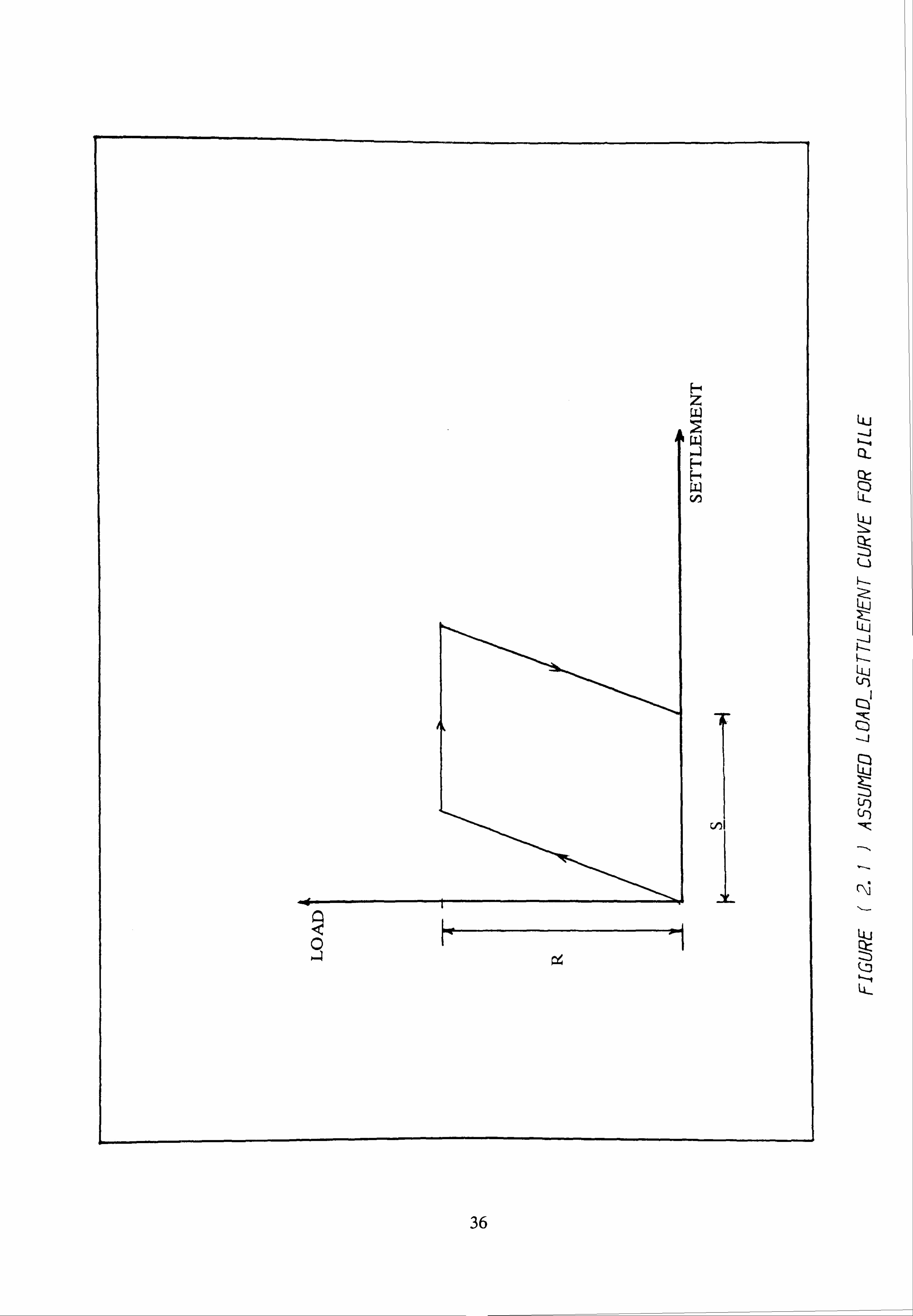
shown in Fig. 2.1, and the process of energy transfer and pile penetration during

one blow of the hammer is shown in Fig. 2.2.

Following Flaate (1964), the hammer energy at impact is:

E, ý ef WH

where,

ef is the efficiency of the drop,

W is the weight of the hammer, and,

H is the height of the drop.

During impact, useful mechanical energy is lost in numerous ways - hammer

rebound, plastic deformation of the capping material, wave propagation through

the soil etc. These losses may be lumped together in terms of a notional

coefficient of elastic restitution n (with reference to Newtonian theory) which

yields an impact energy efficiency factor:

eW+ n2 W

(2.2) gwTwp

where Wp is the weight of the pile.

Because the pile is not a free-body, there is no direct relation between the

intrinsic coefficient of restitution and the notional coefficient. Thus, the parameter

e9 could equally well be assigned some empirical value instead of being computed

16

from equation 2.2.

The kinetic energy of the pile immediately after impact is:

ef e (2.3)

It may be assumed that this kinetic energy is partly dissipated by plastic

work during driving and partly converted into recoverable strain energy. Energy is

also dissipated by propagation of stresses waves through the soil but this (major)

energy loss is invariably neglected in this type of analysis. Assuming, that the soil

responds elasto-plastically to loading (Fig. 2.1) it may be assumed that:

E=R(S+ AS 1

'AS (2.4) PP +2 ep

where,

R is the bearing capacity of the soil, S is the permanent set (irrecoverable downward displacement of the pile

through the soil),

'6S pp is the plastic deformation of the pile head, and,

ASep is the elastic deformation of the pile.

It is by no means clear that the work done during plastic deformation of the

pile head is equal to R. AS pp since the impact force will probably be many times

greater than the soil resistance (dynamic equilibrium being maintained by the

inertia of the pile and surrounding soil). Further, this term may be accommodated

within the impact efficiency factor (eg) briefly discussed earlier.

The third term, representing the stored strain energy imparted to the pile,

which in practice will be manifest by longitudinal vibrations in the pile after

impact, can be recast in the form:

RL ASep =CAEp

where,

(2.5)

17

C is an empirical constant (defined as the ratio between the actual elastic displacement and that given by Hooke's law),

L is pile length,

A is the pile cross-sectional area, and, EP is the Young's modulus of elasticity of the pile.

Equation 2.5 is simply an empirical equation based on Hooke 's law. Combining equations 2.4 and 2.5 we obtain:

(2.6) -A Ep

Introducing the constant:

CL 2AE (2.7)

we obtain the solution:

R=21(-S+J S2 +4aE) (2.8)

or, if elastic strain energy is neglected (a = 0):

(2.9)

These equations and variants thereof are recognizable in the list of

conventional pile driving formulae recorded in Table 2.1. Their diversity is a

testament to their inaccuracy. Further, although some of these formulae are said

to give better results for particular soil types, it is not apparent why this should be so.

18

2.2.3 Discussion

Clearly the pile driving formulae cannot provide a rational basis for analysis

of the driving process. Several investigations have been carried Out to determine

the reliability of various pile driving formulae by comparing the predicted load

capacities with the measured capacities from pile load tests. For example,

Agerschou (1962) showed that Engineering News Record formula, despite its

popularity, was unreliable since it yielded safety factor ranging from 1.1 to 30.

Flaate (1964) investigated the accuracy of the Janbu formula, Hiley formula and

Engineering News Record formula for piles in sand. He confirmed Agerschou

(1962) findings regarding the Engineering News Record formula but obtained

better results with the Janbu formula and Hiley formula. However, pile driving

formulae may be helpful in some cases where local knowledge exists and also as

a means of comparison between piles on a given site.

2.3 SINGLE DEGREE OF FREEDOM MODELS

2.3.1 Introduction

In this section, the pile is assumed to be a rigid mass. The

surrounding soil is represented by a slider-spring mechanism and a parallel

dashpot connected to the rigid mass (Fig. 2.3). The spring deforms elastically up

to a limiting displacement, termed the quake, Q. Thereafter, the slider limits the

spring reaction force. In addition, the increased soil resistance observed under

dynamic loading conditions is represented by dashpot; defined by a viscous

dashpot coefficient, c. This parameter introduces damping into this simple system.

The response of this SDOF system subjected to initial velocity and, also,

cushioned impact is explored in this section. The results of a parametric study of

typical hammer, pile and soil systems are then described.

19

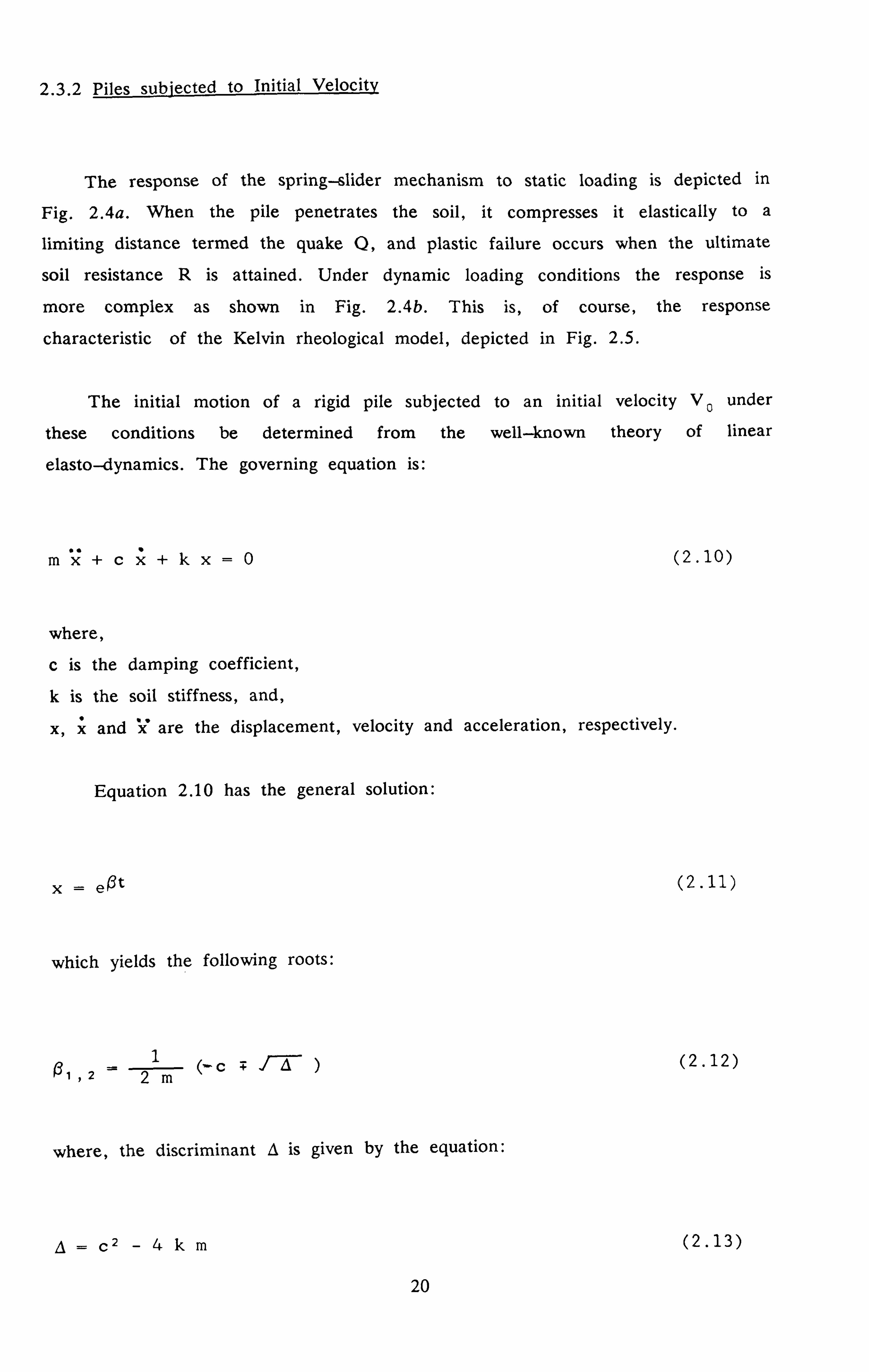
2.3.2 Piles subjected to Initial Velocity

The response of the spring-slider mechanism to static loading is depicted in

Fig. 2.4a. When the pile penetrates the soil, it compresses it elastically to a

limiting distance termed the quake 0, and plastic failure occurs when the ultimate

soil resistance R is attained. Under dynamic loading conditions the response is

more complex as shown in Fig. 2.4b. This is, of course, the response

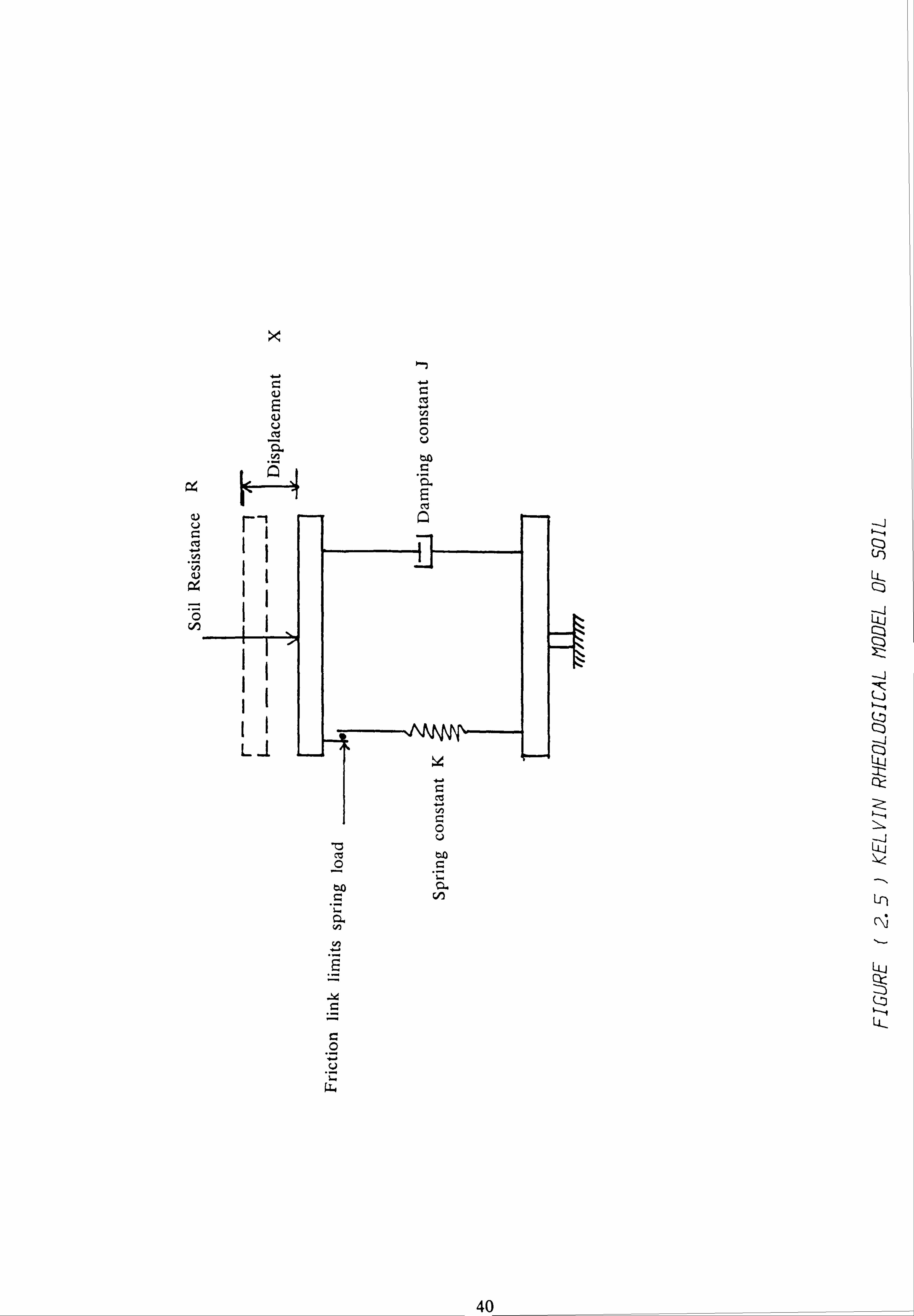
characteristic of the Kelvin rheological model, depicted in Fig. 2.5.

The initial motion of a rigid pile subjected to an initial velocity V. under

these conditions be determined from the well-4cnown theory of linear

elasto-dynamics. The governing equation is:

0" mX+c+kx (2.10)

where,

c is the damping coefficient,

k is the soil stiffness, and,

x, ý and *X" are the displacement, velocity and acceleration, respectively.

Equation 2.10 has the general solution:

eOt

which yields the following roots:

01 ,2ý

where, the discriminant A is given by the equation:

A= C2 -4k

( 2.11)

(2.12)

(2.13)

20

Depending on the magnitude and the sign of the discriminant, three distinct

mathematical cases can be identified corresponding to the physical states of

overdamping, critical damping and underdamping.

Data from Novak (1977) for harmonic loading of axially loaded single piles (and utilised by Randolph and Simons (1986) to develop an improved wave

equation model) suggests that critical damping is a reasonable approximation here.

This conclusion may be verified by calculation based on the following values for

the constants:

. 7r r2L pp

2.9 GL

2w rL (p G) 1/2

where,

r is the pile radius, L is the pile length,

G is the soil shear modulus,

p is the soil mass density, and,

pp is the pile mass density.

This result is in accord with the physical intuition that a pile subjected to

an initial velocity will rapidly come to rest. For critical damping, the

displacement-time relation is:

Ct) e-(g2itn-) (2.14) 2m

Substitution of the initial conditions:

x(O) =0

(2.15) ý (0) = yields

ci=0

C2 ýv0

21

Thus, in general:

Vt e-(Ct ) 02m (2.16)

resulting in the type of motion depicted qualitatively in Fig. 2.6. However, in

practice permanent deformations will occur when the pile displacement exceeds

the elastic limit. At this juncture, equation 2.16 no longer applies. During plastic

pile penetration, the spring-slider model furnishes a constant resistance, namely R.

Furthermore, the viscous resistance reduces substantially since if slip takes place

along the pile shaft, radiation damping into the surrounding soil would be sharply

curtailed. Hence, the magnitude of the viscous coefficient (c) during plastic pile

penetration is likely to be substantially smaller than the values used in equation 2.16.

Consequently, during plastic pile penetration, the response is governed

approximately by the equation:

00 mx+R=0 (2.17)

Choosing a new origin in time/displacement space at the onset of soil failure;

integrating of equation 2.17 yields:

t2

where,

V1 is the velocity of the pile at the onset of soil failure,

t is the time from this point, and,

x is the permanent displacement.

(2.18)

Consequently, the permanent set (maximum plastic deformation) is:

MV12

4R (2.19)

22

Clearly, for practical purposes, equation 2.19 is insufficient since the velocity

V, is not known at the outset. Further, equation 2.16 is not amenable to direct

analytical solution. Recourse has therefore been made to a numerical solution, the

results which are depicted in Fig. 2.7. This shows that the velocity ratio (V 1/V 0) is approximately linearly related to the product cea, where:

ce Q vo c (2.20)

Assuming, the empirical relationship:

Vl 2 uP (2.21) vo

we' Obtain;

4mR( vo -Qmc )2 (2.22)

This result shows that there is some threshold initial velocity below which

pile driving becomes ineffective, typically one or two meters per second. At high

initial velocities, equation 2.22 simplifies after re-arrangement to;

4S (2.23)

Assuming no energy loss at ram impact, this equation can be rewritten, in Janbu

(formula) equation form, as:

WH s (2.24)

23

where W is the weight of the ram and

k+b (2.25) 2b

and the pile/ram mass ratio b is defined as follows:

w b Lp- (2.26) w

Typical values of the pile/ram mass ratio are approximately 0.5 leading to k

values of 1.1 which are similar to those obtained using the Janbu formula.

Further development of this approach would be possible but has not been pursued here since the basic premises of the SDOF model are too simplistic to warrant

exhaustive analysis. In the reminder of this Chapter, the major thrust is the

exploration of a rather more complex model by numerical means as a prelude to

the study of the wave equation method of analysis. This model is superficially

similar to the nonlinear Kelvin model described above, i. e. it consists of a

slider-spring and a dashpot, but there is one important difference; the dashpot is

not independent of the slider-spring mechanism. Under elastic conditions, the

governing differential equation is:

.0

kxý+kx=

where J is the viscosity parameter.

Under plastic conditions, the corresponding equation is:

JR+R *0

where

(2.27)

(2.28)

24

(2.29)

This rather unusual formulation originates from Smith's (1960) work on the

wave equation and may alternatively be described in terms of a "dynamic" soil

resistance (under elastic conditions);

JV) (2.30)

Equations 2.27 and 2.28 are too complex to admit analytical solutions, and,

consequently, an incremental numerical solution based on rigid body mechanics

was developed as follows. Assuming the pile displacement at time t is xt, the

displacement after time increment At is (approximately);

Xt+At = Xt + Vt At (2.31)

where Vt is the velocity of the pile at time t.

This displacement compresses the soil spring resulting in a resisting force R;

xt+, At (1+JV)

The resulting velocity is given by the equation;

Vt+At v+R At tm

(2.32)

(2.33)

Equations 2.31-2.33 form the basis for a simple incremental (in time)

solution strategy. Provided that sufficiently small time steps are employed, the

process is convergent. In addition, in view of the single degree of freedom,

25

computational costs are very modest. The computer program which was used to

generate the results presented in the following section is listed in Appendix C.

2.3.3 Results

For convenience, the model parameters used in the study have been

expressed in dimensionless form as follows. The natural circular frequency of vibration of the undamped system is:

w= ý/ -(

) (2.34) m

Hence, dimensionless time (T) is defined by the product;

(2.35)

Velocities are normalised with respect to the damping coefficient, thus;

iv (2.36)

Displacements are normalised with respect to quake, i. e.

x xQ (2.37)

And, finally, the natural circular frequency of vibration is rendered dimensionless

as follows: .

26

w=w (2.38)

Fig. 2.8 shows the algorithm's convergence characteristics with respect to the

displacement-time relationship for a typical pile. The results show that

convergence is rapid and suggests that useful results can be obtained with as large

as a dimensionless time interval (w t) 0.1. In each case, the following

parameters were assumed, Q= 2.5mm, J= 0-5s/m, m= 2000kg.

Fig. 2.9 shows the algorithm's convergence characteristics with respect to

maximum displacement for three soils (w = 0.05,0.2 and 0.5). Again, the results

converged in each case provided that a sufficiently small time interval (w KO-1)

was adopted.

Fig. 2.10 shows a similar plot for the same pile but in this case, the initial

(dimensionless) velocity of the pile is much higher, i. e. increased from unity (in

Fig. 2.9) to four. Convergence is affected by this change in velocity. However,

the results of the three different soils all now converge to the "analytical"

solution- a solution obtained by assuming that the elastic response of the soil

may be neglected. As expected the "analytical" solution provides excellent results

for piles subjected to high initial velocities since these undergo much higher

(plastic) displacements. however for low initial velocities, pile response is

dominated by the soils elastic behaviour.

Fig. 2.11 shows the pile maximum displacement-initial velocity relationship.

it is clear that greater initial velocities results in greater displacement. Typically,

a fourfold increase in initial velocity causes a ninefold increase in pile

displacement. Under constant force restraint, a sixteenfold increase in maximum

displacement would be expected but viscosity rapidly slows the pile down in the

early stages of pile penetration.

Fig. 2.12 shows the maximum pile displacement--soil stiffness relationship

and, in particular, that these displacement may be very large in soft soils.

Fig. 2.13 shows the time taken for piles to reach their maximum

displacements for various soil conditions and a range of initial velocities. Clearly,

high soil stiffness is associated with fast peak response times as are high initial

velocities.

27

In order to assess the physical validity of this model we consider the

following typical case:

Steel pipe pile; L= 30 m

A=0.01 M2

m- 2400 kg

0) = 288 rad/s Soil; (soft normally consolidated clay)

2.5 mm J-0.5 s/m

Ks = 2x108 N/m

The pile is subjected to an initial velocity V0 of 4 m/s. The corresponding dimensionless parameters are:

amp V=JV=2; w=wQJ=0.36,

and therefore the corresponding maximum displacement from Fig. 2.12 is X/O =

20, i. e. a displacement of 50 mm. This is a rather high penetration and suggests

that real piles would not gain this magnitude of linear momentum.

2.3.4 Piles subjected to Cushioned Impact

Cushioned impact can be treated in the same manner as before except that

an additional mass is used to model the ram and, also, the cushion is modelled

by a spring capable of transferring compression but not tension, Fig. 2.14.

An approximate solution for the forcing function, F(t) supplied by the ram

can be found by considering the mass--spring system depicted in Fig. 2.15. The

governing equation is;

mr x+ kr x (2.39)

28

where,

mr is the ram mass, and,

kr is the cushion stiffness.

Solving, we obtain;

x Vn

sin (cot) w (2.40)

where V0 is the impact velocity of the ram, and,

kr (2.41) mr

Thus, from Newton's second law;

F(t) = Vo 0) mr sin (cot) (2.42)

and, since the spring cannot sustain tension, the forcing function represents a half-sine function. In practice, the peak force will be rather less than VO W Mr since the support (pile) will displace downwards during impact.

OI)timum Time Interval

In this numerical model, the optimum time interval (the largest time interval

which produces an a ccurate solution) is found to be a function of several

variables. Clearly, both the impact and the pile displacement have to be properly

modelled. Assuming a dimensionless time interval of 0.01 ( by reference to the

convergence rate for piles subjected to initial velocities), the optimum time interval will be the lesser of the following:

29

0 0.01

; 0.01 wr

(2.43)

where w and wr are the natural frequencies of vibration of the pile/soil system and the ram/cushion system, respectively.

2.3.5 Results

The parameters which form the basis of the parametric study are as follows:

Hammer; mr= 1600 kg

Vrý 6 m/s (impact velocity)

Cushion; krý6x108 N/m

Soil; 2.5 mm 0.5 s/m

ks= 8xlO9 N/m

Steel pipe pile; L= 20 m 0.01 rf, 2

mp=1600 kg

The corresponding non-dimensional parameters are;

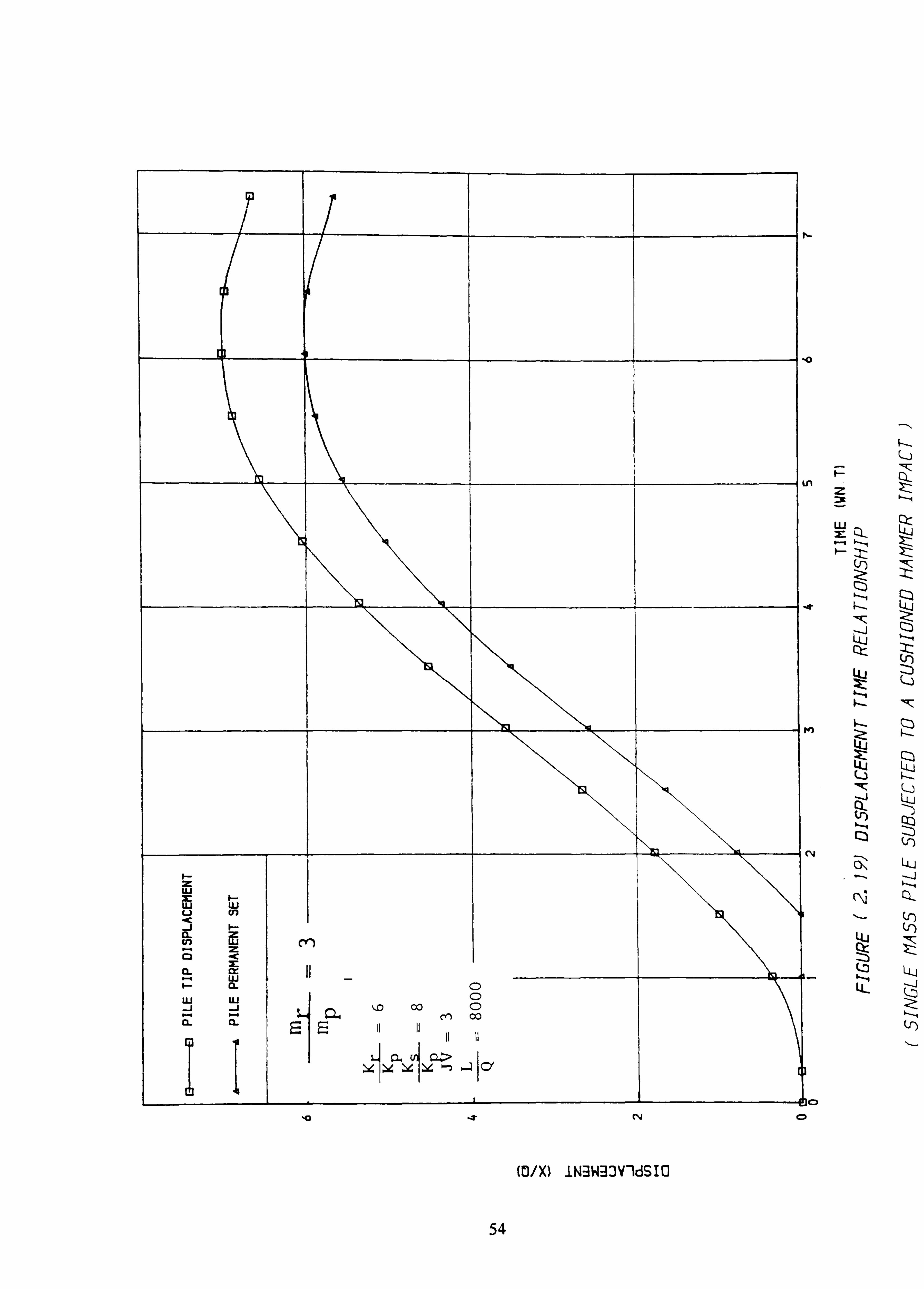
mr/mp = 1, J V= 3, kr/k P =6, L/Q=8000 and ks/k p=8.

The effect of increasing the ram mass/pile mass ratio from unity to three

(mr/mp= 1 to mr/mp = 3) on the peak ram force is shown in Figs. 2.16 and 2.18,

respectively. This large increase of the ram mass causes typically, only a thirty

percent increase in the peak ram force. But this causes a corresponding threefold

increase in the pile maximum displacement (or set) as depicted in Figs. 2.17 and 2.19.

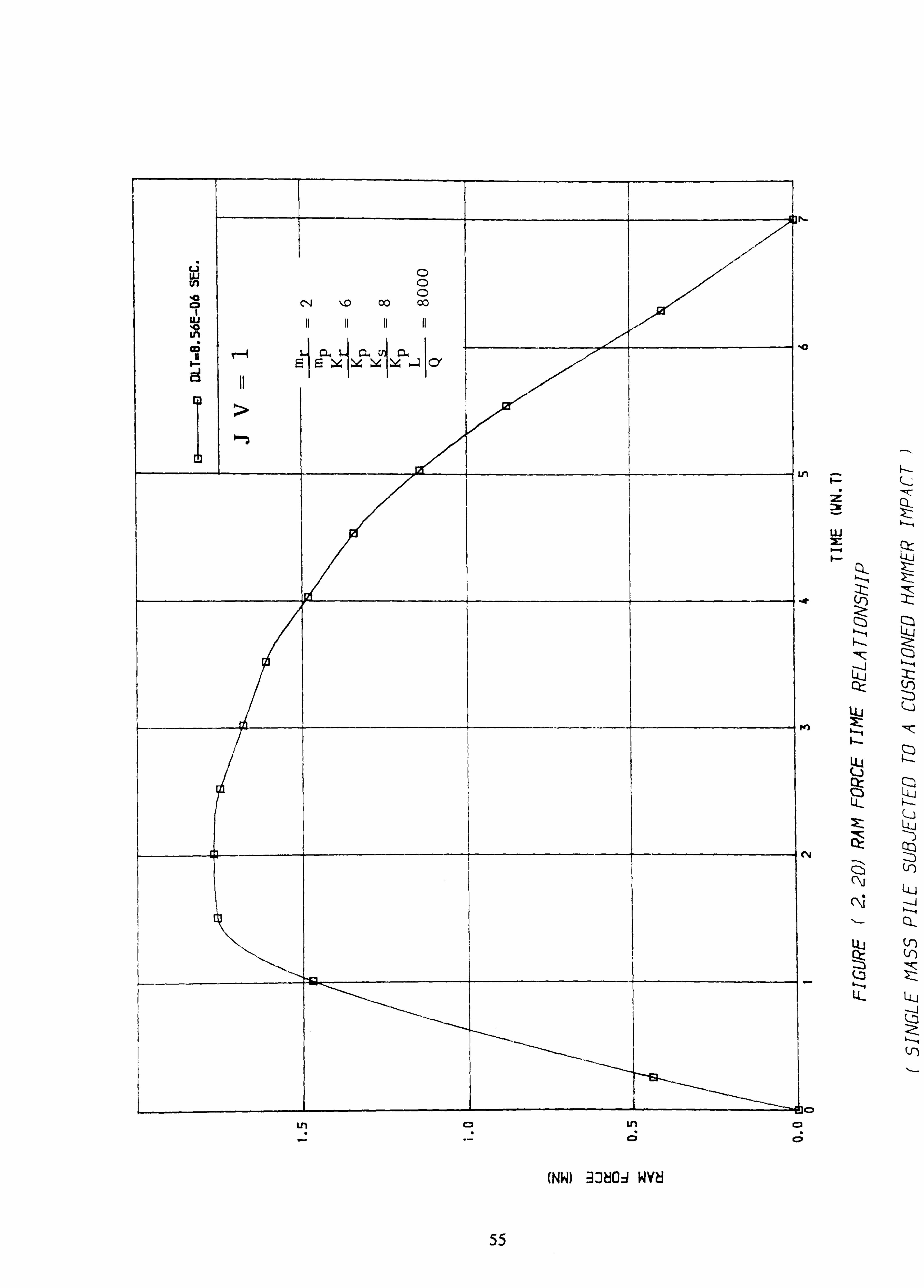
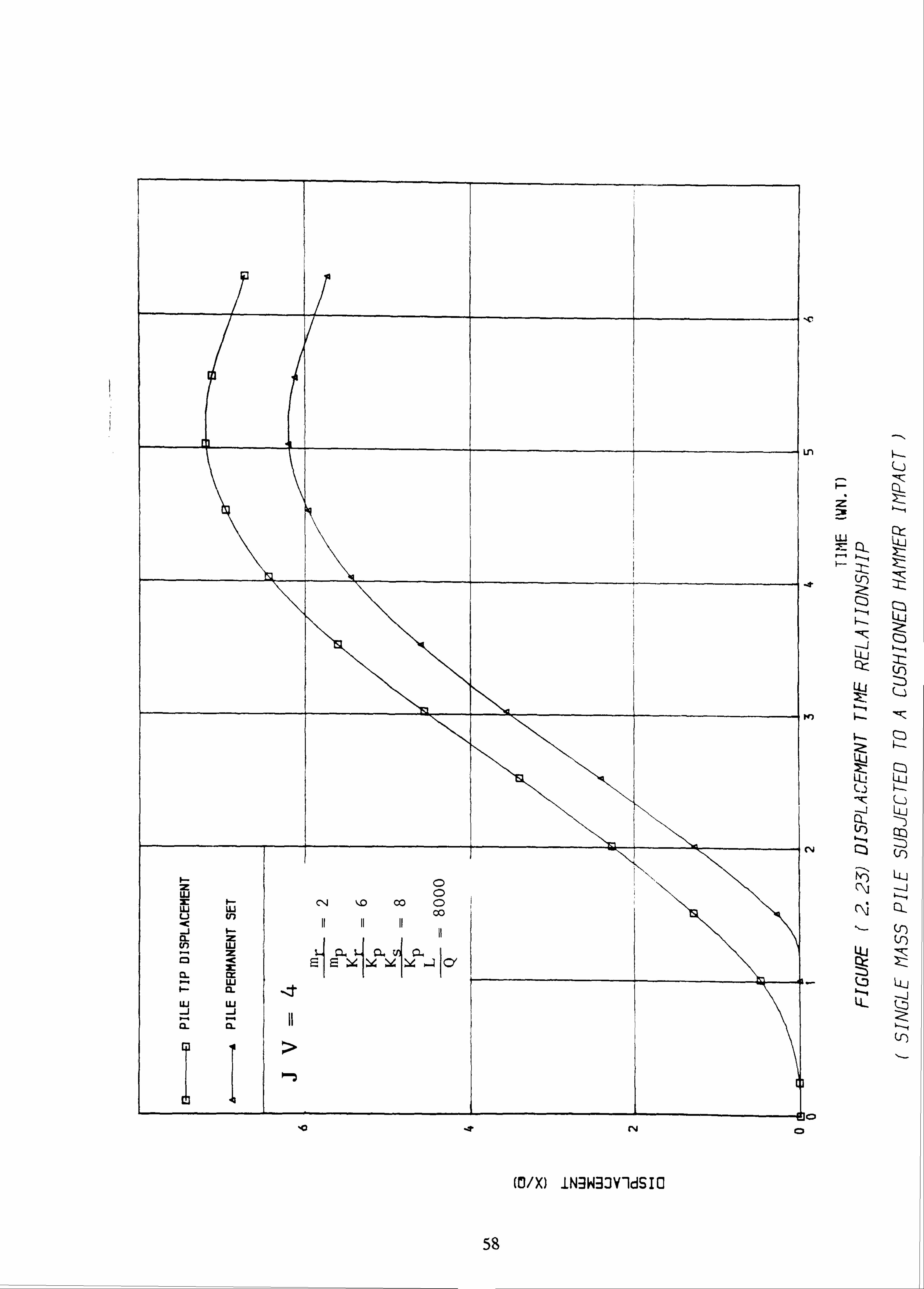
Figs. 2.20 and 2.22 show the effect of increasing the ram velocity from 2

m/s to 8 m/s (JV= 1 to JV= 4), on the peak ram force. This causes a typical

increase in the peak ram force of ninety five percent, which results in a very

30

significant sixfold increase in the pile displacement, shown in Figs. 2.21 and 2.23.

The effect of increasing the cushion stiffness from kr/k p=3 to kr/kpý= 10, on

the peak ram force, is shown in Figs. 2.24 and 2.26. The stiff cushion causes a

typical increase in the peak ram force of fifty percent. However, this only results in a minor increase (6%) in the peak displacement of the pile, Figs. 2.25 and 2.27.

Figs. 2.28 and 2.30 show the effect of driving the same pile in soft and stiff

soils (ks/k P=5 to k. /k p= 10, respectively). The increased soil stiffness does not increase the peak ram force markedly. However, in the stiff soil the pile displacement is decreased by about fifty percent, as depicted in Figs. 2.29 and 2.31.

The effect of increasing the pile length from 10 m to 60 m (L/Q= 4000 to

L/Q= 12000, respectively) on the peak ram force is rather small as shown in

Figs. 2.32 and 2.34, respectively. This increase in pile length (keeping the other

nondimensional parameters unchanged) implies an increase in ram mass in

proportion to pile length and hence a high displacement is obtained as expected,

Figs. 2.33 and 2.35.

2.3.6 Discussion

These simple models are inadequate from the practical point of view since

they seem to yield unrealistic values of permanent set (based on values of the

corresponding wave equation parameters) and fail to capture the complex detail of

pile motion after impact. The results indicate that heavier ram masses and high

ram velocities produce higher pile sets but cushion stiffnesses have only a minor

effect on pile driveability.

31

2.4 CONCLUSION

Pile driving formulae and single degree of freedom models can only provide

very approximate solutions to the pile driving problem because they ignore the

complex interactions that take place between piles and the surrounding soil.

Further, they are based on highly idealised representations of soil behaviour and

neglect wave propagation along the pile and energy radiation into the soil. The

wave equation approach, which is discussed in the following Chapter, rectifies

some of these omisions by taking into account the axial compressibility of piles.

0

32

Formula Equation for Ru Remarks

Sanders WH S

Engineering WH C=1.0 in. for drop hammer

News S+C

0.1 in. for steam hammer 0.1 WpIW in. for steam hammer

on very heavy piles

Eytelwein WH w (Dutch) S W+ WP

Weisbach SAEp

+ 2WHAE

L v/(L-L--ý) +

Riley efWH 0

See Tables 2.2,2 .3 and 2.4 for values S+112(C, +C2+C3) W+Wp

of ef, C, C2 t C3 and n.

JWHý k CdO + -, /-1--+--t-e7C-, j) Janbu u d)

(TIU -S Cd 0.75 + 0.15 Wp1W

ke WH'LIAEV

Danish ef WH See Table 2.2 for ef values.

S+ (2ef4VHL IAEIý) V1

5.6 v4eýg,,, (101S) Units are inches and tons (short).

Gates 4-0 \ýe-ýHTFO 9-1 o- (2 5 IS) Units are metric tons (1000 kg)

and centimeters.

TABLE (2.1) SUMMARY OF PILE DRIVING FORMULAE

(After POULOS& DAVIS, 1980)

33

Hammer Type

Drop. harnmer released by trigger Drop hammer actuated by rope and

friction winch McKiernan-Terry single-acting hammers Warrington-Vulcan single-acting hammers Differential-acting hammers McKiernan-Terry, Industrial Brownhoist,

National & Union double-acting hammers Diesel hammers

TABLE (2.2) VALUES OF THE HAMMER EFFICIENCY, ef (After CHELLIS, 1961)

Pile Type Head Condition

ef

1.00

0.75 0.85 0.75 0.75

0.85 1.00

Drop, Single- Double- acting, or acting Diesel Hammers Hammers

Reinforced Helmet with composite concrete plastic or greenheart

dolly and packing on top of pile 0.4 0.5 Helmet with timber dolly, and packing on top of pile 0.25 0.4 Hammer direct on pile with pad only - 0.5

Steel Driving cap with standard plastic or greenheart dolly 0.5 0.5 Driving cap with timber dolly 0.3 0.3 Hammer direct on pile - 0.5

Timber Hammer direct on pile 0.25

TABLE (2.3) VALUES OF COEFFICIENT OF RESTITUTION, n

(After WHITAKER, 1970)

o. 4

34

(a) Values of C,

Temporary Compression Allowance C, for Pile Head and Cap

Material to Which Easy Driving: Medium Driving: Hard Driving: Very Hard Driving Blow Is Applied Pi = SOO psi Pi = 1000 psi P, = 1500 P, = 2000 psi on

on Cushion on Head or Cap psion Head Head or Cap or Pile Butt (in. ) or Cap (in. ) (in. ) If No Cushion (in. )

Head of timber pile 0.05 0.10 0.15 0.20 3-4 in. packing inside cap on head of precast concrete pile 0.05 + 0.07b 0.10 + 0.15b 0.15+0.22 b 0.20 + 0.30b 1/2-1 in. mat pad only on head of precast concrete pile 0.025 0.05 0.075 0.10 Steel-covered cap, con- taining wood packing, for steel piling or pipe 0.04 0.08 0.12 0.16 3/16-in. red electrical fiber disk between two 3/8-in. steel plates, for use with severe driving on Monotube pile 0.02 0.04 0.06 0.08 Head of steel piling or pipe 0 0 0 0

(b) Value of C. 2 C2 = RuLIAEp

(Include additional value for followers. )

(c) Valuesof C3 C3 is temporary compression allowance for quake of ground. Nominal value = 0.1 inches Range = 0.2 for resilient soils to 0 for hardpan

b The first figure represents the compression of the cap and wood dolly or packing above the cap, whereas the second figure represents the compression of the wood packing between the cap and the pile head.

TABLE (2.4) VALUES OF Cl, C2, C3 FOR HILEY FORMULA

(After CHELLIS, 1961)

35

F- z

F- F- 1J

1

LU

cr_

LC

Q)

Lr (f 11 IK --N

LIJ

36

cu

I

LLJ

LLJ

NO 0ý1

LLJ

Lu

Lu Lit

Q3 LLJ LLj

:ý -- I--- LL, Lj z LL

C3 LO

Irl Cý LLJ

LLJ

U- Lp c)

LL-

37

cc

1

co

Ow

cd

LLJ UJ

t :j

ýLýl Ql) Z! t

LLJ

LL-

38

> C: 0 4ý

E o ' to

cz

10 cl

0 cz

0

cz

CY

-0

(fi

I-l"

LIA

LL-

39

ý4 C) U

cl) C)

ý4

0

x

cz 0

.4 to

CD. cn

0 (-)

40

C--)

(f)

LL-

CZ)

Ed

I -j LIJ

Ln

LL-

C';

Ln

Q,

ý-n Cr)

ui

LLJ Q::

D

Ln 6 \0

LLJ

Q3 LL-

Ln

C3

(3

( WW ) AIWINýdSIO

"i Lm

41

Ln C;

d

9--4 tn 2.

I-

-J

LLJ

0 0

( OA/LA ) ý1130'GA

42

CD Ln 0 Ln (D 0 1%- in N Cl

dddd

-Air C) I

W) 40

I

N Cý C2

uj uj I

lu I

ui

9 9 9 9

44

'0

(DM IN3W33V-WSIO

10

-it

cv

(I- 1-4

Lu

uj

L14 Lu

Cl- V)

LL,

OD LL4

43

T-0

Ln r L 9 ý ý "I

C) C) CD 11 Is

Cý

ýr Ing

C%4

( (0/X) / ([)/X) ) OIIYH IN3W33Y-1d9I0 WnWIXVW

C)

Cl-

(0

LU

LU

:z

C3- U. j X: z

ILI

oc L14

LQ

"'K -K ---I C)- C- (J) i--_, 1-4 Q1 C--

Q CX 44

LLJ "I-'

U-

44

C I-

C

C 1

r'i

I

C

N

( "iý-IVNV (DM / (Offl ) OIIM IN3W33V-1dSIO wnwixvw

C3

Q- 1-4 Z

Qj

- '"Tl-

W cký

_j

uj IL 2:

LIJ L14 M: : Eý lz

U4

pý zi V)

Ul-I

Qr)

LL,

L14

LL- (2

45

A x

C%j

'XYW (C/X) *A iN3W93V-IdSI(I wnwixyw -3-11 d i-

U C3 L474 Lu

UJ _j

-1 C3 CD

46

cn cr) cn (n Z U) ZZZ cn c2 Z 22 CD 23 Z c3 CD 1--- U

12

ýg er 53 01: CL tr CL CL cr

-. i CL

-J -. J AC -A ck -C ci 9 L) u

L) CJ >- W >- ci: >- 92: -i w -i -i LU cZ -c AK gg

ZZZZ cZ

0000-ý

cx 9 10 R

(CM IN3W-33Y-IdSI(I 3-lId wnwixyw

:X 11

1209

Er) Or) LLJ

U- LL

p.,

0

CN

C;

0

0 0

CD

47

» >; - :> : ', ': o 2? .. 3 c2 Z CD CD ., (Z 9-4 CD o" c2 e- oý 1-- L) L) e- Li

ti ci Li c21

@ c2 ui c3 tr UA 12: LU ct: LU

CL XM CL er

_a CL CL

< i er i - - Li ti ýc W _9 u Li 9--4 0--4 e-- b4 2i >- Ir >- x

-. i L -i ui

-. i LU

-c 3: -c x: -< x:

x" zxl/

// Z

CD W)

c2 rY

Cl

U*NA) iN-3W-33V-IdSI(I WnWIXYW iY NU

Ln Cl- F-4

1-4

LLJ

QQJ

(n J s-, LU :z Cý3 C: ) U- U- cn

CZ, LL,

i Ql

4: 3 11--t Lu U)

LL- LL- C2

C

C

C

48

TEXT CUT

OFF IN

ORIGINAL

cil on

U,

49

V) VI 03

E

Q-1

Qý

C)

50

Zt

Ct Lk,

LL,

Qj

Qj 111Z 1-4 C:: )

Qj CC) LLJ Lu C3 Lu

Cý LLý 1-6

LL,

0 CD

ID 00 0 cn 00

ui L;

ff)

10

10 w

ca, oor

-a, m (N -

(NW) 3380=1 WY8

uj X:

LIJ

Q--

LL, CY

Q

LU Q,

LL

bq! )c) cz

"K QL

P: Li7ji

I, <

LLJ

51

w Z: f-- ui ti

ui cn

«C -i i- CL (n

m Ui

c2 -c CL

3: cr LU

w

CD CD CD

"0 Co 00

El C%j

(CM IN3W33T1dSICI

CY

. &D

CD

I-

ui M: cl-

V)

LQ Qr-I U-j

W Z LQ

V) Q

LU

Q3

LL

52

L3 LU in

CD CD CD

%10 00 00

CD Uli n

CY')

c2

%a -T CN

(NW) 9380: 4 WV8

f-

-0

P Ln 2i

: 3r

LLJ 2:

Lu Z

LLJ

Cj LL

C%j

LLJ

LL-

bloc, Cp

53

uj uj uj u cn

in uj cy") 0 -C

CL x

ix ui

CL

ui -i

LLJ -1

C) %10 00 0

a CL CL C l cn 00

10 -e rY

(D/X) iN3W33Y-ldSIO

10

Lfl

-41

14)

C%j

ul = izL- I .. 1 ý-. 4

V)

ct LLJ

LU

Q- , U) C: )

L-U

L3 ,, --I LL

54

tn CD CD

10 0 CD

C-4 1. -0 00 00

ui

CID el 1. i CY r=

Ln C3 Ln C) CD Cl

(NW) 3J8O=l WY8

p

2i : 19

LU

-Z

.. --i LLj Cl--

uj

Lu Q Ct C- Zi Lt-

z

Q)

Lu

ILO ,, --I LL

55

0 cl-j \10 00 0

uj uj 00 u Zn

th ui Ei

I

CL CL

ILJ a_

C3 Ln 6

(C/X) iN3W-33V-ldSIO

56

a

X:

Lu

LL,

It's LL-

Lu I-

, IZ

P

CQ

L4-j

-j

QL

V) V)

LQ

J ul cn %a CD I ui V

U! 0 0

CN 00 00

IG 4t ri

(NW) aJdO=l HY8

Qt

C14

-MCD CD

LLJ

Ztz (A) k- c: i

Lai Z

Lu Qj

U-1

LL

57

ui m uj ui u cn

C%4 11.0 00 0 00

CL z to ILJ z C3 . 1c 3c ý4 u Cy CL cr

LLJ

ui LU -i a- CL

10 4t r4

(O/X) iN3Wg3VldSIO

le.

Ln

-4.

K)

-ela CD

-73

LU

U-j Qr- Lu

L

cl, U) Q)

LLJ

LL

58

L3 uj

10 CD

uj %C CY) i

co C) i 0 0

C-1 00 00 O-

C3 m Z

I- CL>

2r'

'T en (J

(NW) 9JHO-J WV8

ýc

.0

(14

13

CD

2

LLJ

I H

LLJ z 1-4

LIJ

LQ

Q'i L--, LL

59

lsý

uj ww u Ln . -C

U. j C3 -C

CY) X: uj 1

LLJ LU -j

C14 00 00 CY)

wl -0 M (N

(O/X) iN3W9JV-ldSIO

'C

CY

-19(D C)

F-

i

LLI c)

-__j Lai cr- 41 Z

Lu

Ln

LL,

LL

QL

Qr_ LQ

LLJ

Cý ( r)

Cr) V) TZ: LLJ

60

LLJ vi

V

tu 10 11 0 Ln I C14 00 cf) 00

Cl. -j

13

14) 'T N

(NW) 9380A WY8

41

0

oflol Cl

LLJ M:

Qr) Zt

-j LLj Qr- U. j z

Lij Q Qý Cý LL

1.0

Ltj

U-

61

uj 2c LU uj u tn c -i I- a- LLJ C3 -C

CL cr uj

tu uj

CL CL C) 0 0

a 00 cn 00

-ýr Pr) CY

MIX) iN3W3JV-ldSI0

-T

m

C%j

-Eic, Cl

I-

uj

LE

LL

Li

I Q-)

LLJ

d Zý (J)

62

: 39

(NW) aJdOJ WVd

ui x:

Zý Q) i-I

. --j

Lu

Lu u

UL . Cý)

41

V) LU

CL

LLJ

-j

63

ýT N0

CD CD CD

CY) 00

ui uj U-j U (f)

CL Lo LLJ

M Ir ui

I. - CL

Lr) uj

-i LLJ

-j i

03

('4

(13/X) IN3W3JY-ldSIO

4.

C%j

-imc) cnl

I-

z

LLJ

(. 0 Zil

ct

ZL

Q- U-) Q)

EZI

LU

LL

r-t-

LLJ

P QJ

QL

LQ

64

Qj Ql-

(NW) -3J? JO-J WV6

LLJ M:

ýItz ,j

LU z

LU u Or C) LL

I

'I:

C:: 4

Q-)

LQ -j 1-4 Q-

LLJ

65

10 -4 r4 CD

Cý-

X: (ý, - Lu

LLJ C. 1- LI. J

It'Ej CZ)

ca

LU

V)

LLJ

LQ

( O/X ) IN3W: l3V-ldSIO

66

-T to CV C)

C-j 110 co CY)

L; ui

CD

uj co ca C

C) 0

C),

,a -Z N CD

(NW) 3380ý WV8

LLJ 1:

U-j Q Cz LL

LU

Cl-

(. r) V)

Lu

67

C%d

LLI X: I. - LLJ ui u ul c

-i n- x U') LU C3 -C xC

uj

LLJ LLJ

110 co CY)

PL>

CDI

Ln CDP Ln C) I C; C;

( 13/X ) INN-33VIdSIO

2i

LU X: Cý- LLJ

LLJ

Q-)

LLJ

LLJ

1 :

t:

s C: ) LLJ

, --" --i U-

68

C) 0 0 C%4

ui (n C14 %lD 00

CY)

tn CI) ui co - Q. a> Ea ýZlu u-I U

o-

-41 ('J

(NW) 3380: 4 WV8

3ul

Zt LU

. Cýr-

CZi Z5

Cd

Q)

Q: cz

LL Lu

tJo 0

69

(NW) 9380-J WV8

70

Co v CN4

CHAPTER 3

THE WAVE EQUATION MODEL

3.1 INTRODUCTION

3.2 FORMULATION

1 3.2.1 Discrete Equations

3.2.2 Critical Time Step


3.4 RESULTS

3.4.1 Wave Equation

3.4.2 Comparison with Elementary Models

3.4.2.1 Wave Equation versus SDOF models

3.4.2.2 Wave Equation versus Pile Driving Formulae

3.5 DISCUSSION

3.6 CONCLUSION

CHAPTER 3

THE WAVE EQUATION MODEL

3.1 INTRODUCTION

The elementary single (rigid) mass models described in the previous Chapter

provide some insights into the behaviour of piles during driving. However, due to

pile compressibility, real piles respond in a more complex manner to hammer

blows. In particular, there is a time lag between the occurrence of the hammer

blow at the pile head and the arrival at the pile toe of the resulting compressive

stress wave.

Smith (1960) proposed an idealisation of the hammer, pile and soil system

which is capable of representing the passage of the stress wave down the pile, (refer to Figs. 3.1 - 3.3). In this idealisation, the pile is modelled as a series of

discrete rigid masses connected by springs (which act in both compression and

tension). The surrounding soil is represented by a set of slider-springs connected

to the rigid masses. These springs deforms elastically up to a limiting

displacement, termed the quake (Q). Thereafter, the slider limits the spring

reaction force. In addition the increased soil resistance observed under dynamic

loading conditions is represented by a dashpot ; defined by a viscous damping

coefficient, J. This parameter introduces damping into the system. The hammer

ram can, similarly, be modelled as a discrete mass (or masses) and the cushion

by a spring capable of transferring compression but not tension.

A numerical solution of this system, based on the solution developed by

Smith (1955,1960) is described in this Chapter. The results of a parametric study

of typical hammer, pile and soil systems are then described and these are

compared with those predicted by elementary models. Some useful relationships

were obtained from this work which form the basis of a new formula (in the

form of a "pile driving formula") which may be of some value in practice.

Application of this pile driving formula to full-scale pile load test results from

the North Sea yielded encouraging results.

71

3.2 FORMULATION

3.2.1 Discrete Equations:

Smith (1955,1960) showed that the "discrete equation" solution of the wave

equation was simpler to implement than the usual (at that time) finite difference

strategy and with very little modification this approach is still used to date. For

completeness, the main steps are outlined below.

Let the displacement of any discrete mass at time t-ý- At be denoted by

Xt-f- At. Assuming constant velocity Vt during the time interval At, then:

Xt +At = Xt + Vt At (3.1)

If the displacement of a second (adjacent) mass is denoted by the superscript

prime (') then the compressive force between the masses ff') is,

I X- (3.2)

where,

K is the spring constant, and,

the subscript (t-+. - At) has been dropped for clarity.

The resultant force P due to pile compression acting on any particular mass

is the sum of the spring forces acting above and below it, i. e.

P= 'f + f'

=K( 'X - 2X + X' ) (3.3)

72

where the pre-superscript prime denotes the second adjacent mass.

Clearly, equation 3.3 will require modification at the pile head and at the

pile toe (refer to Figs. 3.4 and 3.5). The external resisting force due to

the soil is denoted by the symbol R where, by definition, under elastic conditions:

R= Ks X(1+JV)

where

Ks is the soil stiffness, and, J is the viscosity coefficient.

During soil failure (X> Q), the soil resistance is limited to,

R= Ks Q(1+JV)

(3.4)

We note that viscous damping (under elastic conditions) is assumed to

increase with increasing soil displacement, a departure from classical rheological models.

The resultant force acting on a typical discrete mass is, therefore;

P+R

from which the mass accelerations and velocities can be determined. Thus,

Vt+At ýV+F At

tm

(3.5)

(3.6)

Equations 3.1 to 3.6 form the basis for a simple incremental (in time)

solution strategy. Provided that sufficiently small time steps are employed, the

process is convergent. Further, in view of the small number of degrees of

freedom, computational costs are very modest and, consequently, great

73

sophistication in deriving more efficient algorithms is hardly warranted.

Fig. 3.6 shows a typical displacement-time relationship predicted by this

method. In the figure, the permanent set of the pile is indicated by subtracting

the quake from the pile tip displacement.

3.2.2 Critical Time Step:

Smith (1960) pointed out that the greater the number of discrete masses in

the model (i. e. the shorter the "'unit length" of pile modelled as a discrete rigid

mass) the smaller must be the time interval, At to avoid numerical instabilities.

Fundamentally, during each cycle of calculation, the stress waves must not travel

further than one discrete mass length. On the other hand, reducing the time

interval much beyond this limit serves only to increase computational costs but

without any increase in accuracy.

The speed of wave propagation in the pile is essentially equal to the uniaxial

wave speed (c), i. e.

c=f(E)

where,

E is the Young's modulus of elasticity, and,

p is the mass density.

(3.7)

If n discrete masses are used to model a pile of length L, then the critical

time step is:

Atcrit ýnLc (3.8)

74

or, in terms of discrete quantities,

At crit (3.9)

where m is the discrete mass:

(3.10)

where A is the pile cross-sectional area, and, K is the spring constant:

EA L

Using either equation 3.8 or 3.9, the critical time step can be readily evaluated

within the computer program and an appropriate time step can be selected.


The value of the quake, Q, used in this study is taken to be 2.5 mm, following Smith (1960), Hirsch et. al, (1970), Goble and Rausche (1976), Coyle

et. al, (1977), Goble et. al, (1980), although, Authier and Fellenius (1980) have

proposed higher values of quake (8 - 20 mm), (see also Hannigan, 1984).

Some workers, for example Litkouhi and Poskitt (1980), have assumed two

different values for the viscous damping coefficient J; one for the pile tip and

one for the pile shaft. Typically, the former is assumed to be one third (1/3) of

the latter. In this study, a single value of viscous damping is used (0.5 s/m) for

75

simplicity, following the work of Yip and Poskitt (1986). The optimal time interval

used in this analysis is found from convergence tests based on the critical time

interval defined by equation 3.8.

In what follows, the influence of the major parameters in some typical cases is explored and the results are presented in dimensionless form. In most cases,

subdivision of the pile into ten (10) discrete masses was found to yield results of

sufficient accuracy.

3.4 RESULTS

3.4.1 Wave Equation

Fig. (3.7) shows the displacement-time relationship of the pile head of a

typical pile subdivided successively into 2,4,8 and 16 discrete masses. The

results show the rapid rate of convergence and suggests that useful results can be

obtained with as few as eight elements. The ramforce-time relationship predicted

from the numerical calculations is approximately a half-sine curve, similar in

shape to that given theoretically by equation 2.42. However, the peak ramforce

generated by impact on a compressible pile is well below the corresponding value

predicted for impact on a rigid pile (Fig. 3.8), as might be expected.

The typical hammer-cushion-pile and soil system parameters which form the

basis of the parametric study are as follows:

Hammer; mr = 1600 kg.

Vr ý6 m/s (impact velocity)

Cushion; Kr ý 6xlO8 N/m

Soil; (a very stiff highly over consolidated clay)

2.5 mm

J=0.5 s/m

76

Ks = 8xlO9 N/m

Pile; L= 20 0.01 M2

2xlOll N/M2

8000 kg/M3

1600 kg

The corresponding non-dimensional parameters are:

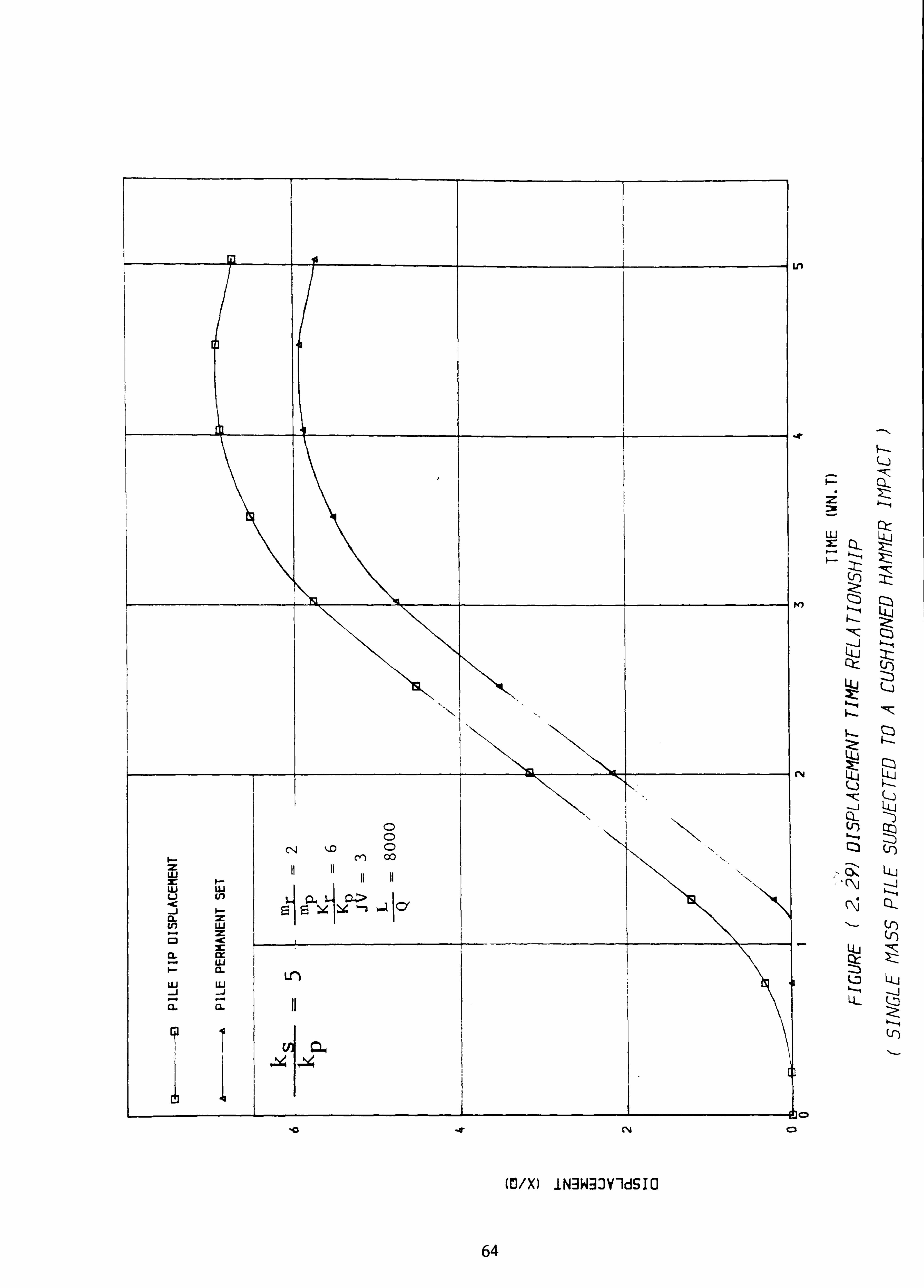
mr/mp = 1, VJ=3, Kr/K p=6, L/Q = 8000, Ks/Kp = 8.

The effect of increasing the ram mass on the peak ramforce is shown in

Fig. 3.8 and 3.10. An increase of the ram/pile mass ratio from unity to three,

causes, typically, a fifty percent increase in the peak ramforce. Moreover, using

the heavier ram, the pile displacement (permanent set) is typically eleven times

greater than that produced by the lighter ram. Figs. 3.9 and 3.11 show the pile displacement-time response.

The time taken for the pile to reach its maximum displacement is typically

forty percent longer for the heavy ram compared with that for the light ram.

This is largely due to the fact that the displacements are much greater in the

former case. Clearly, in practice heavy ram masses may be necessary to attain

adequate penetration and these longer times (to reach maximum displacement) are

inconsequential in comparison with the duration of the loading cycle.

Figs. 3.12 and 3.14 show that an increase in the ram velocity from 2 m/s

to 8 m/s results in a seventyfive percent greater impact force and this increase in

ram force increases the pile set by , typically, eighteenfold, Figs. 3.13 and 3.15.

Figs. 3.16 and 3.18 show that a stiff cushion (Kr/K P -10) causes typically a

twentyfive per cent increase in the peak ram force, compared to that using a soft

cushion (Kr/K p =3). The effect of this increase on the pile displacement-time

relationship is shown in Figs. 3.17 and 3.19. The maximum displacement (and

set) using a stiff cushion is typically ten per cent greater than those predicted

using a softer cushion.

77

Figs. 3.20 and 3.22 show that an increase in soil stiffness (from Ks/K P=5 to

KS/Kp= 10) increases the ram force by, typically, one hundred and fifty percent. Further, this increase in the soil stiffness reduces the pile displacement (or set) by typically fivefold, as shown in Figs. 3.21 and 3.23. It may be noted that this

change in soil stiffness increases the time taken for the pile to reach its

maximum penetration.

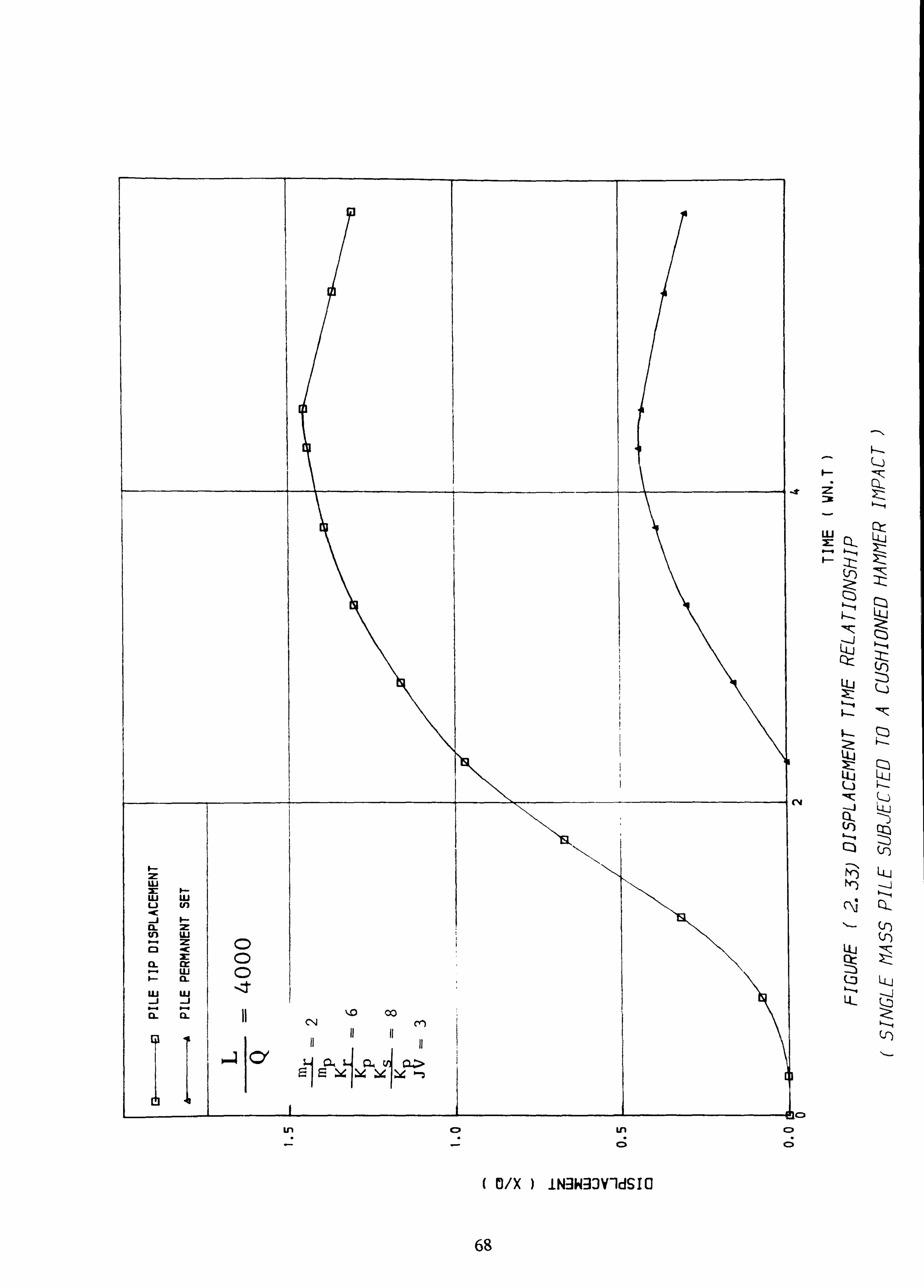
Figs. 3.24 and 3.26 show the ramforce-time relationship as a function of the

pile length. Here the pile length is increased from 10 m (L/Q= 4000) to 30 m (L/Q= 12000) which causes a typical decrease of twenty percent in the peak

ramforce.

Figs. 3.25 and 3.27 show the displacement- time relationships of short (L/Q= 4000) and long piles (L/Q= 12000) driven in the same soil. The maximum displacement (and set) of the longer pile is typically thertyfive fold greater than

those of the short pile. However, increasing the pile length does not result in any

significant change in the time taken for the pile to reach its maximum

penetration.

Figs. 3.28 and 3.29 show that if a pile's length is increased, but keeping its

mass and stiffness (Kp) unchanged, the maximum ram force and displacement are

unaffected.

The effect of an increase in the pile stiffness (Kp) on the ram force-time

relationship is shown in Fig. 3.30. For a stiff pile, the peak ram force is

typically five percent greater than that for a less stiff pile, driven under the same

conditions. Fig. 3.31 shows that the pile moves vertically as a rigid body some

time after ram impact. This should be contrasted with the motion with for

example Fig. 3.27 where considerable compression of the pile takes place. It may

be inferred therfore that very stiff piles undergo rigid body motion.

In all cases, it may be observed that the piles reach their maximum

penetration after the ramforce has reached its peak value due to the inertia of

the pile--soil system.

78

3.4.2 Comvarison with Elementary Models

3.4.2.1 Wave Equation versus SDOF Model

In this section, results from the single degree of freedom model (SDOF)

are compared with those obtained from the wave equation (MDOF) analysis. The

same parameters (excluding pile compressibility in the SDOF model, of course)

are used in both models.

The effect of increasing the ram/pile mass ratio from unity to three

(mr/mp=l to Mr/mp =3) on the ramforce time relationship is shown in Figs. 3.32

and 3.34, respectively. The peak ramforce obtained by the SDOF model is

typically eighty percent greater than that predicted by the MDOF model for light

rams. But this increase is typically sixty percent for heavy rams.

The effect of ram/pile mass ratio on the pile displacement-time relationship is shown in Figs. 3.33 and 3.35. The pile set predicted by the SDOF model is

typically two hundred percent greater than that predicted by the MDOF model for light rams. However, this increase is typically twenty percent for heavy rams. Further, the pile set predicted by the SDOF model are typically sixty percent

greater using the heavy ram while the increase predicted by the MDOF model is

ninety percent.

The effect of increasing the ram velocity from unity to four (VJ= 1 to

VJ= 4 i. e. the hammer velocity increases from 2 m/s to 8 m/s) on the ramforce-

time relationship is shown in Figs. 3.36 and 3.38, respectively. The peak ram-

force predicted by the SDOF model is typically fifteen percent higher than that

predicted by the MDOF model for the slower ram and the peak ramforce

predicted by the SDOF model is typically seventy percent higher than that

predicted by the MDOF model for the faster ram. The increase in hammer

velocity causes an increase of three fold in the peak ramforce, predicted by both

the SDOF and MDOF models.

79

Figs. 3.37 and 3.39 show the pile displacement-time relationships predicted

by the SDOF and the MDOF models. For the slower ram, no permanent pile

displacement was predicted by the MDOF model while a relatively small pile set

was predicted by the SDOF model. On the other hand, pile set were predicted to

increase sixfold by both models when the piles were driven by the faster ram. However, the pile penetration predicted by the SDOF model is typically fifty

percent greater than that predicted by the MDOF model in this case.

Figs. 3.40 and 3.42 show the ramforce-time relationships for two cushion increased stiffnesses (Kr/K P=3 to Kr/K P =10). In these figures, the peak ramforce

predicted by the SDOF model is typically sixty percent higher than that predicted by the MDOF model (for the soft cushion). But, the use of a stiffer cushion

causes an increase of sixty percent of the peak ramforce obtained from the SDOF

model but no remarkable increase is predicted using the MDOF model.

The influence of increasing the cushion stiffness from Kr/K p=3 to Kr/Kp= 10

on the pile displacement-time relationship is shown in Figs. 3.41 and 3.43,

respectively. The pile set predicted by the SDOF model using a soft cushion is

twice that predicted by the MDOF model. Using a stiffer cushion has little effect

on pile penetration.

Figs. 3.44 and 3.46 show how the ramforce-time relationship is influenced

by changing the soil stiffness from KS/Kp=5 to KS/Kp=10. The peak ramforce

predicted by the SDOF model is typically sixty percent higher than that predicted

by the MDOF model in driving into a soft soil. The effect of soil stiffness on

pile set predicted by the SDOF and MODF models are shown in Figs. 3.45 and

3.47. Driving piles into soft soils yields virtually the same results by both models.

However, pile penetration into the stiffer soil is predicted to be much less by the

MDOF model. Clearly, SDOF models are only valid when piles are relatively

rigid compared to the surrounding soil.

Figs. 3.48 and 3.50 show the ramforce-time relationships obtained from the

SDOF and MODF models as a function of the length (keeping other non-

dimensional parameters unchanged); specifically from 10 ra piles (L/Q=4000) and

30 m piles (L/0=12000). The peak ramforce predicted by the SDOF model is

typically fifty percent higher than that predicted by the MDOF model for the

80

short pile. The increase in pile length causes a decrease of thirty percent in the

peak ramforce predicted by both models and the peak ramforce predicted by the

SDOF model (for this long pile) is sixty percent higher than that predicted by

the MDOF pile model.

Figs. 3.49 and 3.51 show the effect of increasing the pile length on the

displacement-time relationships. For short piles, some penetration is predicted by

the SDOF model but no permanent penetration is predicted by the MDOF model.

A summary of these different effects is shown in Figs. 3.52 to 3.56. In

these figures the pile tip displacements as predicted by the MDOF model and the

corresponding sets are plotted for comparison with the results predicted by the

SDOF model.

3.4.2.2 Wave Equation versus Pile Driving Formulae

The pile set predicted by the wave equation method for a wide range of

parameters is depicted in Figs. 3.57 to 3.61, plotted against ram mass, ram

velocity, cushion stiffness, soil stiffness and pile length, respectively. Also shown in these figures are the pile driving formula predictions based on equation 2.6

(after some re-arrangement):

s= eg efW H_1 ASep - ASPP R2

where, S is the pile permanent penetration (set),

W is the weight of the hammer,

H is the drop of the hammer,

R is the ultimate load capacity of the pile,

e9 is the efficiency of the drop,

ef is the efficiency of the hammer blow,

Sep is the elastic compression of the pile, and,

(2.6)bis

81

S pp is the plastic compression of the pile.

and,

ASep CRL AEp (2.5)bis

To permit a proper comparison to be made, no ram losses are allowed and

plastic compression of the pile is neglected; hence the only outstanding variable is

the pile compression parameter C. A range of values is assumed in these

comparisons but it may be seen that th e curves predicted by this approach intersect the wave equation results at a sharp angle indicating that the two

methods can not be easily reconciled (Figs. 3.57' - 3.61).

Examination of the results obtained from the wave equation model and the

pile driving formula suggests that a good match may be obtained if it is assumed

that pile compression and set are related by the empirical equation (Fig. 3.62):

1+0.5 s Q

Denoting the effective work done by the hammer by the symbol E the

permanent set can be re-written as:

(3.12) K

where Kp is the pile stiffness (A Ep /L).

Noting that:

R=Q Ks (3.13)

82

and introducing the soil/pile stiffness ratio (n), where

Ks (3.14) Kp

and the parameter -y, where

(3.15) 4

We obtain after some manipulation (and dropping the subscript p from the

symbol Kp for clarity), the equation:

SK -y +/ (S K y) 2+2EK (3.16)

This new "pile driving formula" may not be of universal validity since it is

likely that the coefficients in equation 3.16 are a function of some parameters

which were held constant during this study; notably the viscosity coefficient J.

The principal unknown in this equation is the parameter y but this may be

estimated from the following equation:

16xl. 06 N/m)

s Q3/ 2

derived from the data given by Authier and Fellenious (1980).

(3.17)

The new "pile driving formula" can be re-written in dimensionless form as

follows:

Ry+/ -y2 +2E

SKK S2 (3.18)

83

The predictions of this equation are shown in Figs. 3.63 to 3.66 and are

compared with the original wave equation results. The effect of increasing the

ram mass, ram velocity, soil stiffness and pile length on the pile displacement

(set) are shown in Figs. 3.63,3.64,3.65 and 3.66 , respectively. As expected, the new "pile driving formula" reproduces these results very well.

Fig. 3.67 shows the pile set as a function of work done by the hammer as

predicted by equation 3.16. If the hammer rating is known and the pile set is

measured, this figure can be used to determine the soil's ultimate resistance.

The relationship between ultimate resistance and the work done by the

hammer is shown in Fig. 3.68. The results are plotted from equation 3.18.

Again, given the rating of the hammer and the pile set the ultimate soil

resistance can be determined. Fig. 3.68 shows that the greater the relative soil

stiffness (n=Ks/Kp) the greater is the ultimate soil resistance.

Fig. 3.69 shows the ultimate soil resistance versus the pile penetration (set)

(or number of blows per meter penetration)for a typical system, as predicted by

equation 3.16. For a given hammer rating, the greater the relative soil stiffness (n= Ks/Kp) the lower is the pile penetration.

Fig. 3.70 shows the relationship between the ultimate resistance and the pile

penetration (set) (or number of blows /meter penetration). These sets of curves

are predicted by equation 3.16. It may be seen that the greater the soil resistance

is the higher is the required rating of the hammer to reach a given set. Also, a

specified soil resistance may not be reached by hammer of low rating.

Fig. 3.71 shows also the relationship between the ultimate resistance and

the work done by the hammer predicted by equation 3.18. It may be seen from

this figure that the greater the soil resistance the greater must be the hammer

rating to attain the requisite set.

In order to test the applicability of equation 3.16 a comparison between its

predictions and the full scale data obtained by Forehand and Reese (1964), shown

in Fig. 3.72, has been carried out. This figure depicts ultimate resistance versus

set and shows that the predicted ultimate resistances were typically ten percent

84

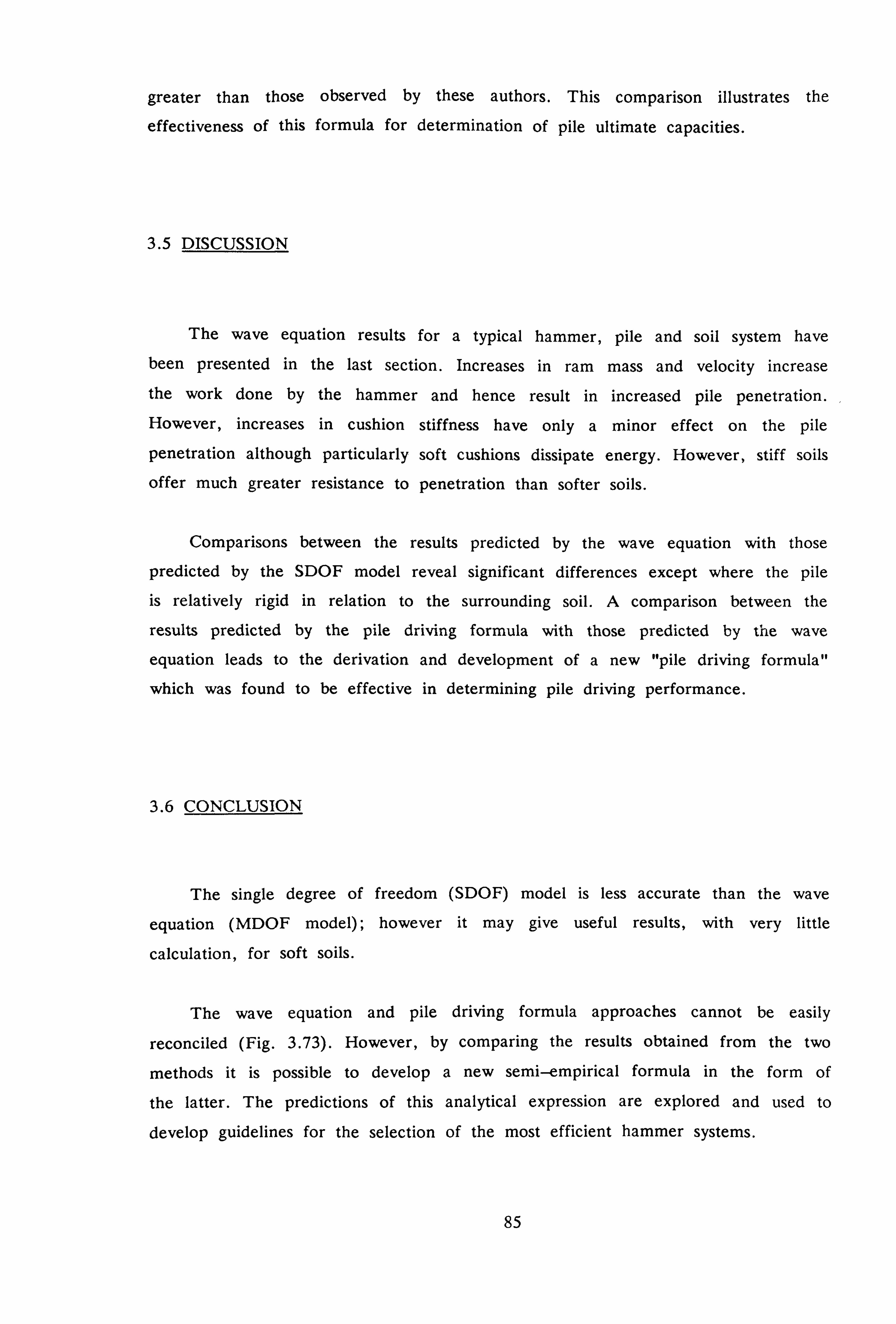
greater than those observed by these authors. This comparison illustrates the

effectiveness of this formula for determination of pile ultimate capacities.

3.5 DISCUSSION

The wave equation results for a typical hammer, pile and soil system have

been presented in the last section. Increases in ram mass and velocity increase

the work done by the hammer and hence result in increased pile penetration. However, increases in cushion stiffness have only a minor effect on the pile

penetration although particularly soft cushions dissipate energy. However, stiff soils

offer much greater resistance to penetration than softer soils.

Comparisons between the results predicted by the wave equation with those

predicted by the SDOF model reveal significant differences except where the pile is relatively rigid in relation to the surrounding soil. A comparison between the

results predicted by the pile driving formula with those predicted by the wave

equation leads to the derivation and development of a new "pile driving formula"

which was found to be effective in determining pile driving performance.

3.6 CONCLUSION

The single degree of freedom (SDOF) model is less accurate than the wave

equation (MDOF model); however it may give useful results, with very little

calculation, for soft soils.

The wave equation and pile driving formula approaches cannot be easily

reconciled (Fig. 3.73). However, by comparing the results obtained from the two

methods it is possible to develop a new semi-empirical formula in the form of

the latter. The predictions of this analytical expression are explored and used to

develop guidelines for the selection of the most efficient hammer systems.

85

However, the major weakness of both the wave equation and this new "pile

driving formula" lies in the use of fictitious soil parameters which cannot be

determined from conventional soil tests.

A more realistic soil model is therefore needed which incorporates non-linear behaviour of soil in a rational model of dynamic soil structure interaction. The

most promising method for accomplishing this task is the finite element method.

86

0

C,,

Cq* . 4-0 V5 02

Ln

fA

-. E S--

-F) "a

co

Ei V 4-

çrj

4-

c)

87

Qý -_j

LL-j

LL,

-j U-j

LQ

LL-

Cýj

Qj crý LLJ

C%j

88

TEXT CUT

OFF IN

ORIGINAL

LQ

I -W_ \-----I

---a. ___________ -'

<\I

__

U-j

--i IM,

"ZIZ Li- C: )

LQ LLJ

89

mole

CY

Ln Lfý Oll

I -_j

--N

N4r

LIJ

90

LU 2i (f) N-4 CZ LLJ

ýZ--

1

(-)

116- +

Q) Z!: &--I Or CL (f) Lu

Cl- -i ý: tz

-, (1) LLJ Lrl cr)

S- LU

91

Z

z4 ' >j > Z, ö

:3 CL4

Z ý4 cy

12. d

CD

INHWEDV-MSIG

c

Q)

W Ct Q-

j LLJ :zC: ý Lo

C3 LQ LIJ

LLJ

11 uj

11-4 LLJ -i -1

-_j Q ýL-

110 LQ

Lu uj

In

92

z Ld Lij -j uj

ul

uj

U-. )

LLJ w uj LLJ 15

uj i LU -j ui

u u

X

tn

cr

U- L3

j

C3

-3. c

r*j

C;

(WW) IN3W-33Y-ldSIO (0V3H TlId) iNgW-3-19 iSdI-J

L;

ui U')

LU x: 0--8

cl:

LLJ z

Lu Q) Or Cýj LL

LLJ

LL

49 CD

Cl

Cý

93

I-

x:

Ot

co

lyi

LQ

?s

(NW) 3380=1 WY? J

94

ýo

LLJ En

LU x 92 m ui LLI ui

uj LLJ -C x r--l I

U. j w

-1 CL CL CL

0 0 C: )

00 00 C11 CL4 CL 1

11

-e W) N

( O/X ) IN-3W33V-IdSIO

-0

-ot

N

4! )cnl

C)

LLJ X:

-_j LI-I 2r:

uj Z b--4

W

r. L (0

czi

fr

LU

LL

95

uj X: Q-

Qr) Zt C: )

LU CL-

LLJ Q. )

-1ý1

Lu

SIS Q) &--q LL-

INW) 93HO-J HYd

96

10 _T r. 4

x

e r4

\-- Co

ui x: X

1

ui ui LL

ui LU =

CL c2: 92 i i

. CD - Ui rn

LLJ LU LL CD -3 --1 --1 00 CD - 2 cl. CL CY) Co

cm 10 ýt r%d (D

( O/X ) iN]W]3Y'ldSIO

_731t

LU x Ll-

--I LQ

LLJ Z

L

LL, Q

-_j Cl-

LLJ 11C

Es "-4 LL-

97

in- ui V) V)

C C

C14 00 C 00

ui

CL 0. (A 0. I'.

u 0.4 ICY

cz ý5 in 1 ' Q Jý

4 to

.4

po (N

(NW) ý3? 30-J WYb

98

co

-0

-e

CN

ISO ID

z

LU x

I -_j LU Ot

LLJ

Qt C 2

LIJ

llý :5 b. --4 L-L

ui LLJ

LLJ ui -. 1 -3 ui ui

£2- KL 0

CD Ir-i CD

1 - e-- 00 CD ui LU 11

il il Co

(N

( OIX ) lN9W33Y-IdSIC

aD

'0

r-4

49CD

z

LLJ m

ILO

l< -_j LIJ Ct LLJ

CL ILr) I--, Q)

LLJ

LL

99

(0

. -i Lij Oc uj 7Z

LLJ Q

U-

0 fn

Lu

( NW ) 9380-J WY8

100

c> 10 PO CD

ui e- Ul

U. i

ZW Z- ui ui ui Ed -i Z

ui ui w -i -i -i '

CD CD CD

c"i %. 0 00 Co CL CL

>

0 CD 10 Qt

( DIX ) lN3W33V'ldSlO

r1i

130,

ui

10

Lu z

LL

5c)

0

101

z

LLJ

Q-

l< --i U-i C)::

(NW) 3380-J HYd

LLJ Z

U. j u ct Q) U-

I Pei I, - LLJ

IQ:

102

ýo -t ry CD

LLJ

LLJ LLJ 1

3: X: :7 ui LLJ LLJ CY) -i uj -i LLJ

CL CL X: cr 0

0 LU CD 1. - 0- 0 1 ui LLJ ui C14 CO CY) 00

I

i a F- ý4 ý4 ja I

ýv 4r rY

( C/X ) IN3W93V-IdS10

103

%a

PO

-IBCD Cl

I-

uj 2: Q-

Co

Zý

LU

Q--

LLJ z

LLJ

z

LU

Q)

-_j Q-

Lr)

a

LLJ

LL

D.

z

LLJ

v (. r)

--_j

uj

LLJ

4-

LL

Cý

(NW) 3380=1 WYd

104

rY C), 10

LLJ En

LLJ uj x X: uj uj uj

uj uj -< X:

0- CL cr

C) Ul 0 I-- a- C LU uj ui -i

0 C14 co 00

Cl- cn

El

10 -r

( UX ) IN3W33V-IdgIG

C%j

0'

.0

re)

ýma Cl

I-

z

UJ m

(. 0

LU Qz-

LU :t

Lu z LU

Lo

C: )

LL

105

: 3t

LLJ x

ZZ

. --j

LLJ

LU

LL

C\j

Lu "I

9s ý-q Ll-

(NW) 9360=1 WY8

106

aD 10 r rý

uj zz

uj uj -i -i z uj uj -C CL Cl. cr

LL) Ln

ui LU uj 0 C)

CL CL C) C14 I'D 00

cn

Co 10 r

( DIX ) INN33Y-1610

10

M

Jo 0

z

LLJ 6- X:

.. -j uj- Qý LU z

Lu

C: -)

C\j

fr;

Q3

LL

107

LLJ V) (n

LLJ

<

co

EU Ol

10 -t N

( NW ) 3380-ýWYd

108

,0 gý

uJ

-4r

N

0

uj uj LU

CL

C14 CD CL CL (Y) 00

,a -W

( O/X ) iN3W3JY-ldSIO

rq

0

CM

I-

:: v

LL Z: c2-

cz

LAJ Z

LI-4

L Lo CZ,

tyi

uj

Ll-

. -Jo D

109

M ui V) tn c I

tlo

ui -j CL

ac C (U C bD

C-1 110 00 CY)

ýv -e C%j

(NW) 9380=1 WV8

-0

-0

r-4

424=1 Co

:x LU

cr LLJ

Lu Q Oc Cý U-

LU IC,

=s LL

110

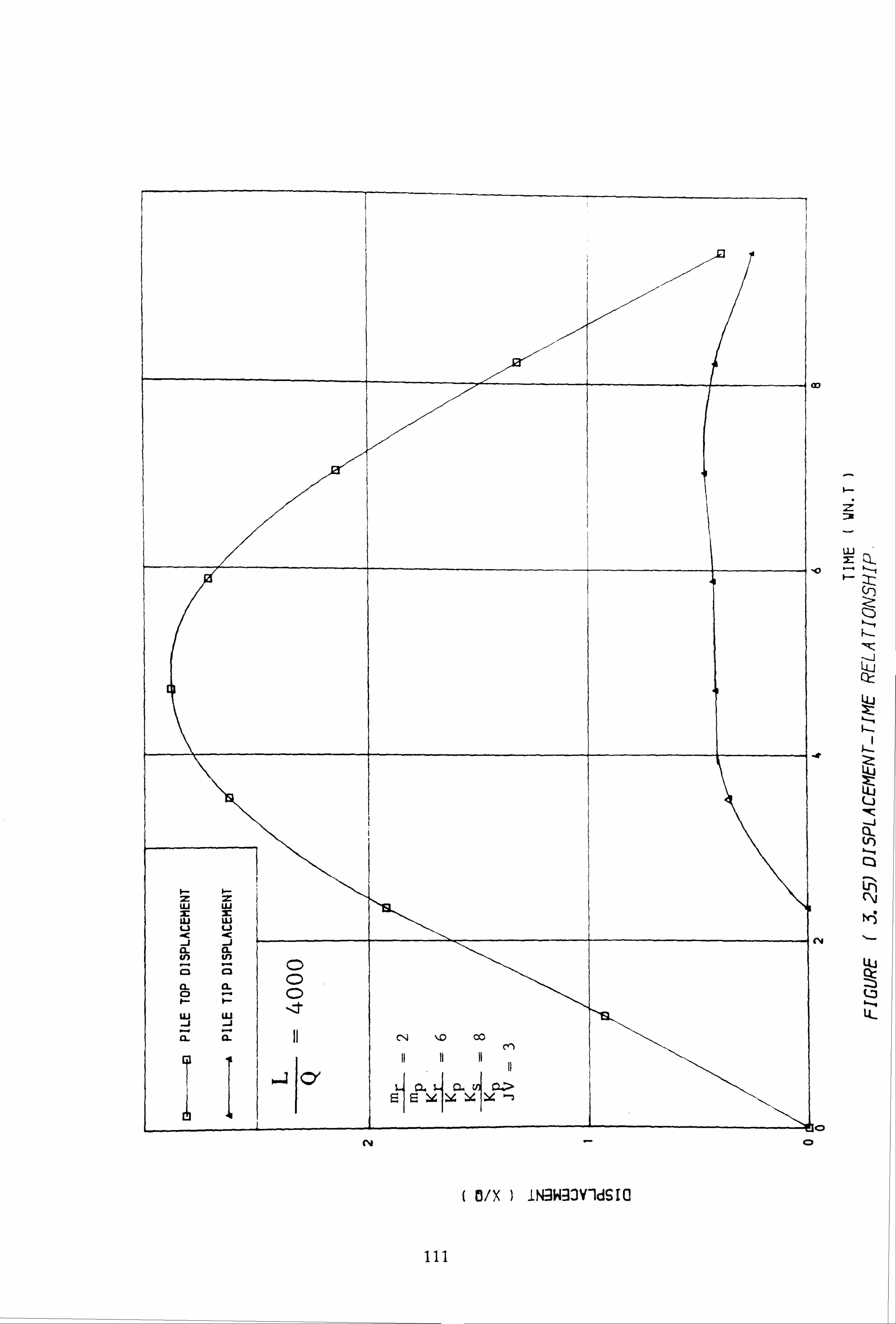
4m

Ic

x ui x

2: uj u LU 4) Ul u

CL CL

to 0 C3

0 CL CD

0. - 0

ui -j

ui -j

CL a- C14 ý-o 00 CY)

( O/X ) AgW-33VIdSIO

Cp

z

U. j

-j LU Qý

Lli Q

U. j

LL

ill

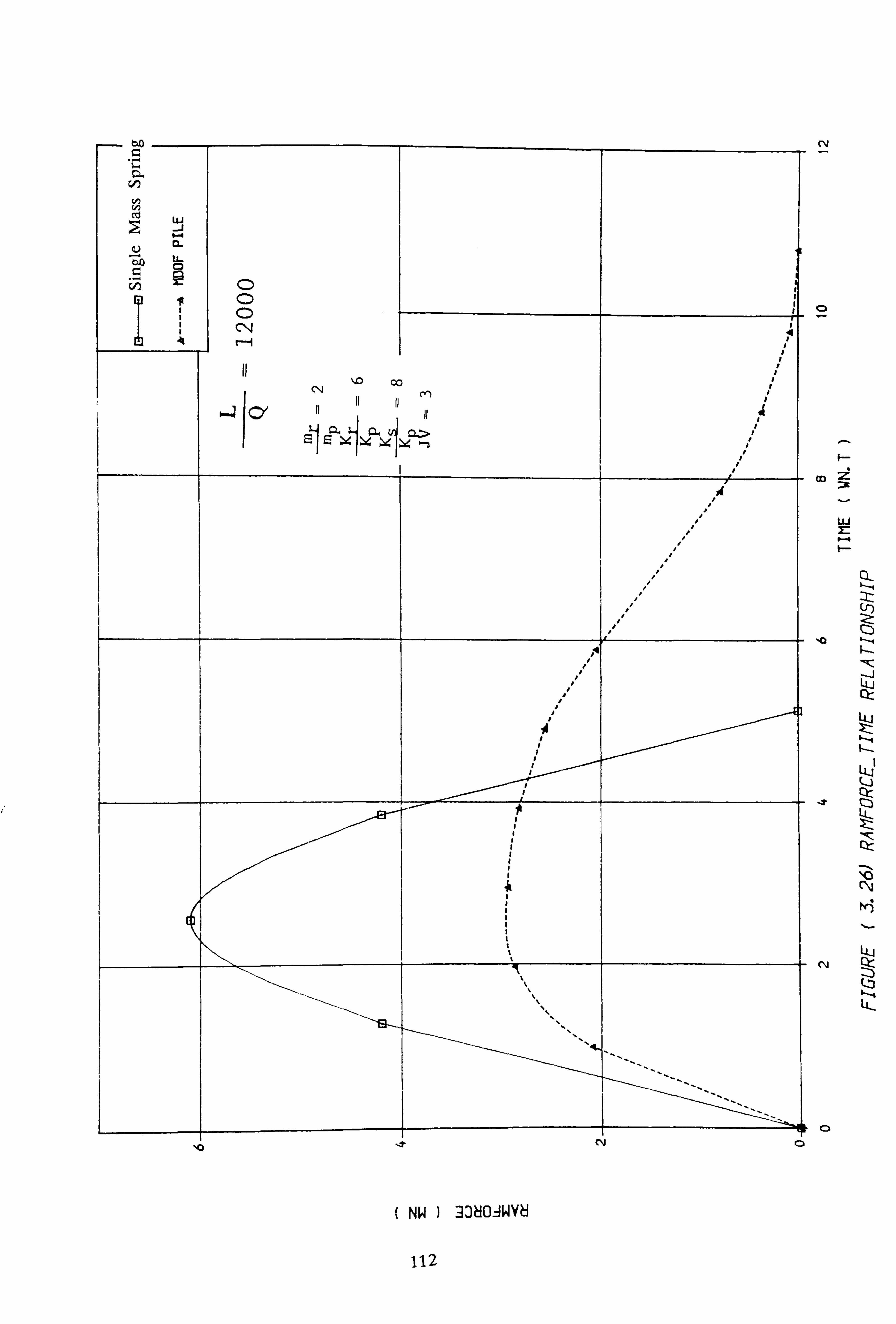
F

Q.

uj

-1 t4 U-

C) C CN

CN 00 (n

C), 11 11

o- Ei . 1.4

10

CV

( NW ) 3380=IWYH

112

C%j

0

oo

LU

b--4 F-

10

-zr

Q-

V)

Lu Qr- LJLJ

L14 I

LU

Q-j 1-4 LL-

Cl

0

Nt,

u j x IC C) LU

CN

I- CL

11.1 L4 6-4 *. 4 6-4

CL a- Q-

11

\10 co

CY) I

('3 I

Cl I co %0

( DIX ) IN-N33VIdSIC

It CV

Ck

LU

=

IT,

. -i LQ c 1-1

. -0

-N

"0

0

L14

1-4

Lti

113

3

10 111 cn ul

13) I. -N

(A "0 co ul 4) 0)

ct

CLI LLJ b6o

0.4 +.. ) c

11 C14 110 Lr)

CI. l ý4 -ý rz Eu ý4 U

CID e 4r

(NW) 9380=1 HV8 I

114

N

10

(N

ISO Cl

LLI x

Q-

LLJ

dLl

Ct

2 Z

LL,

U-

/

X,, 4)

co 1. -1 71 Q)

llý

co

I. - I-- uj U') 0

0 \1

ul

ui

uj

LLJ

X:

(U

(A a. 0 I. - a- a: LU CL

LU Uj LU C) 0 CD CL 0.

C14 Ln

I CY -ý

I

E Eip-ý4 -, j

Co ýo -e

( an ) IN3W33Y'IdSIO

115

(14

ýo

-or

1 r1i

I

C) CD

z

LLJ

LQ Qr LLJ z

Lai

CL Lr)

Q)

uj

7

-r

(NW) 3380-J WY8

116

: 29

Lii x

Lu

uj Z

Q Cr LL "E:

LLJ

Co 10 dr (Ni CD

LLJ tfn)

d5

ul U-1 -C 3c

10

Cd CL ti. cr C3 Lu

Ujj

4)

- CL 0- M

lz I (L)

Co 10 -r

( O/X ) lN3W3OV-IdSIO

117

N

ýc

-4r

N

-inc) Co

z

LU - X: Cý-

Or- uj

UJ Z LIJ

lyi

I- L-Li

?s LL

CD CD CD

%Z 00 Co

-4t K) CY

(NW) 3360=1 WVb

ýo

-0

C'4

0

:X

uj

118

CL 93.

00 00 CY)

F. E 11 -j

Icy

cly

( O/X ) LN3W-33V'ldSI(J

0

At

C%j

"I0 0

LL

Lu X)t

iý

lyi I-

LL

119

CY)

11 110 00 0

m 00

CIO

-40 -it

(NW) ; 33? 10: 1 WV? J

N

N

10

K)

NOD 0

a

:z V) Z:

cd [a-_,

LLJ Q Cc

120

CL CL. III

\D 00 0

cyll 00 EE .4

101

e -A@, cw

(NW) lN3W93Y-IdSIC

121

N

2

0ý

LL

-_j

tý

ýg

LL

L 0

0 CD

C'4 I'D 00 C

00

Ln 0 S

(NW) -30b0=1 WVb

Ln c;

(D

10

-t

C%j

'Ia 0

d

w

LLJ Qc

e

%Z NI

0

LL-

122

cu 0. r--q

CD CD

C"i 110 00 CD

> 00

11

13

.j Icy 0 Ln

C3

-gr

-E)c

0

( O/X ) iN=--IW=I3V-IdSIO

6

S

z

uj 2:

"Irl- --i Lj-j Qr-

Lýk 1-4

Z

LIJ

QL

I-I

U-

123

CD 11 CD U

cli \ID 00 OD j 1

"- l ,'- 1a-1 11

r= u W. w- (Z, ,

P-

e

(NW) 33dD=l WYb

W)

10

tn

41cl C)

: 3t

LLJ

C: L ý--4 Z

1-4

U4 c

LL

124

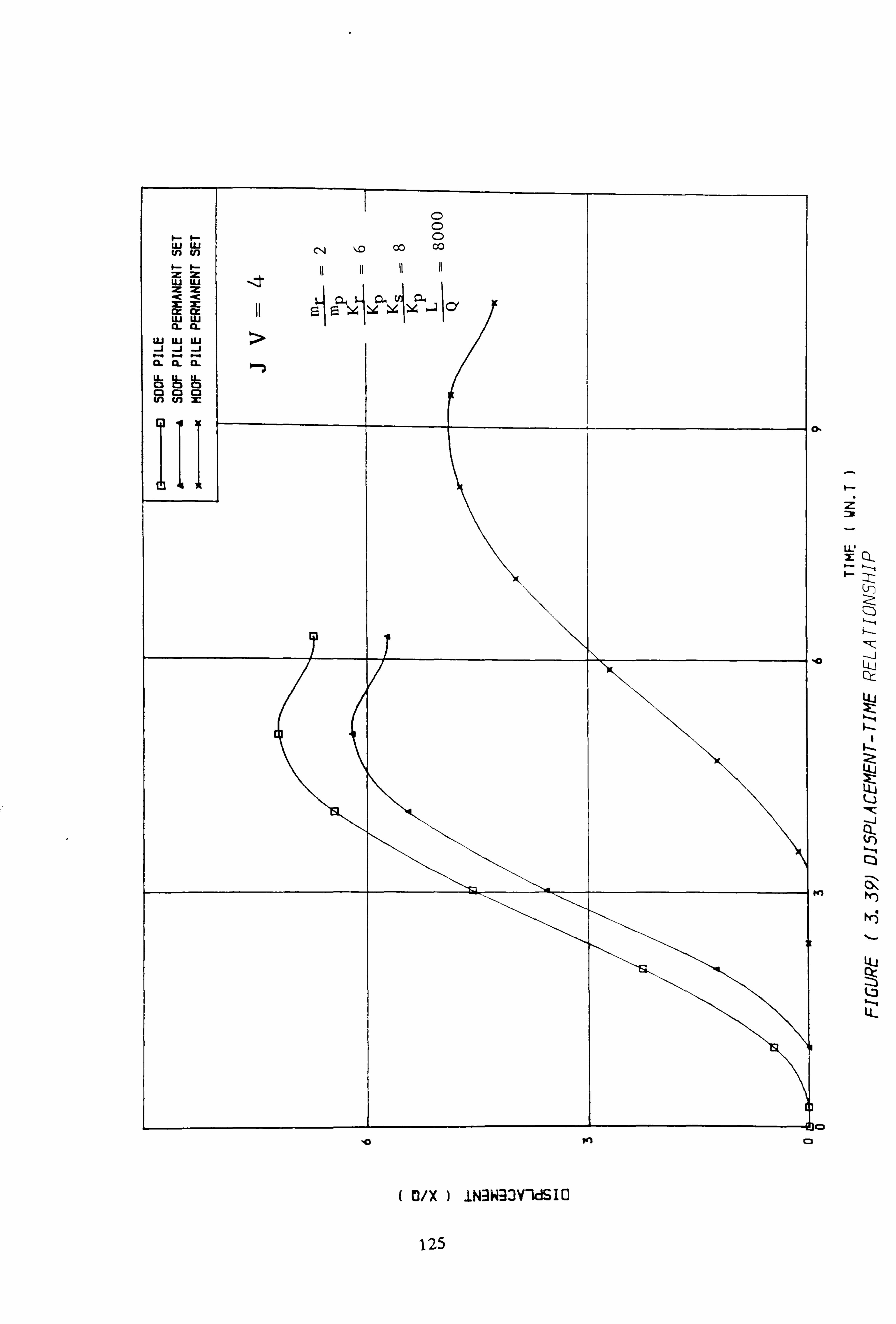
uj in

uj

uj in

uj

C-) C 0 00 C14 00

z Ac x cc

ui a.

LLJ ul

= -C x

cr

ui CL

ILJ

Q4 04 0.

CL IL

68 CL

8 C3 0 cn (n

C3 3c

to .1 it

'0

( 15/X ) IN3W33V-IciSIG

rn

Ok

*0

te)

-MC3 Cl

z

LL2 x (ý-

LQ z

uj Z

QJj

LIJ

?i 6-4 LL-

125

LLJ LU -j -i

C) 0 0

C%4 00 00

CL CL

U- U- 0 C3 C3 C3 in

> o-

S Ul u Ol

-r mi (4

(NW) 3380=1 WV8

CD

LU M:

ýo

-41

(14

Nac) Cl

LLJ Cý-- LQ

Q: C) LL-

LA. j

126

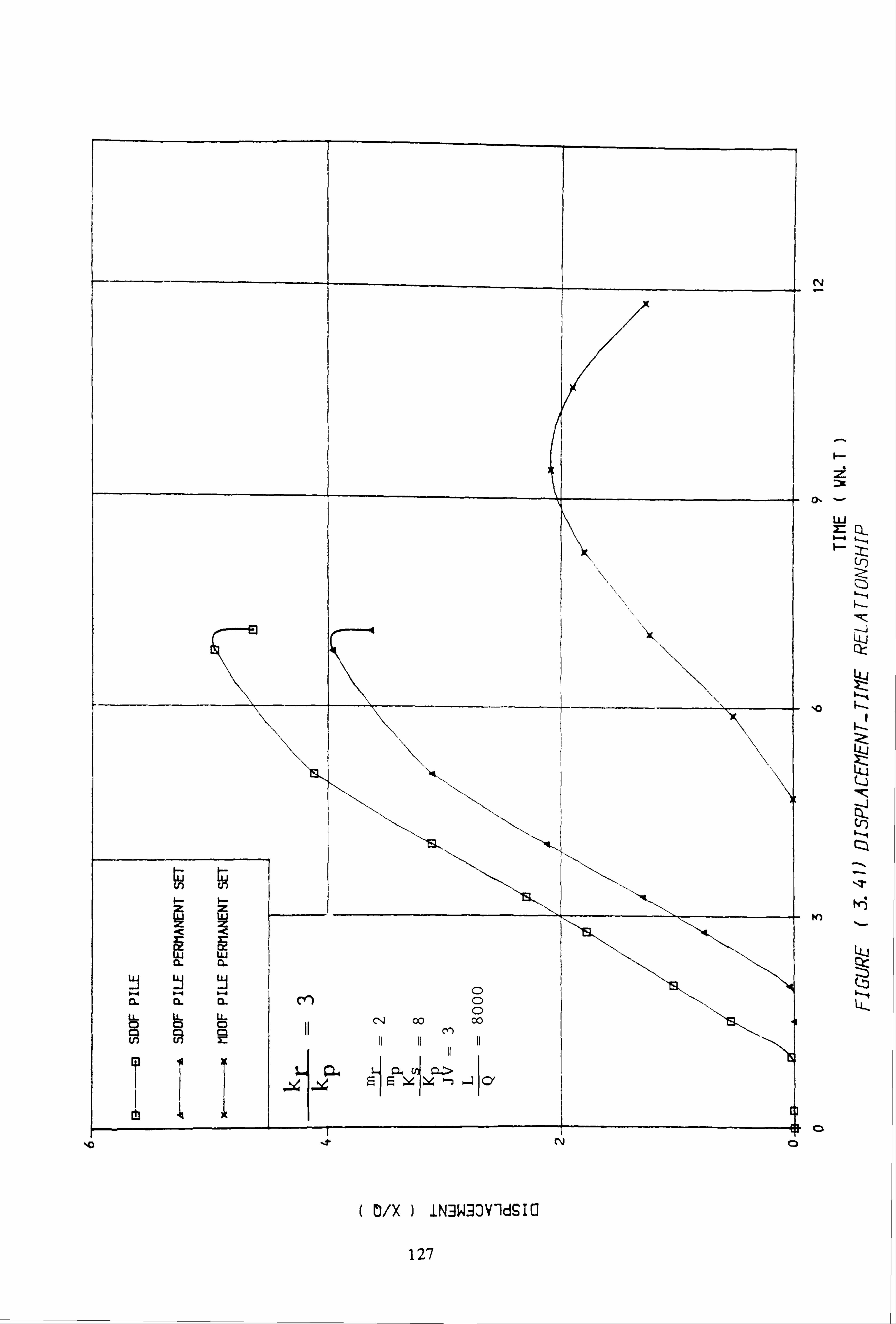
El

LOU

Cl. LH

LL.

$-. d

LL. a

CY) 00 00

CV)

CY E ý4 ý4

10 %t

( O/X ) ANKY-ldSIO

EN 0

N

: )g

uj = C)_

LL

SO

W)

0

CZA

LLJ

127

uj uj -j -i

0 C14 00 CY) 00

CL a.

U- U-

C W

> rz ý4 u CX

10 -dr

(NW) ; 3380-J WV8

CY

w

ýc

-gr

r-j

mmo Cl

=

ui m

cl-

:: r_ V) Z:

LLJ Or-

LIJ z

LL

Lij

It's L"

LL

128

ui LLJ CD ul Z CD w ui ZZ CD

CD c -c x: Z CI-3 Co 00 cr cr ul LU CL CL

ui ui -1 3 - - c2. CL> CL 0» 5Xx -5 Ei U- LL (D (2 C: ) c2 c2 c3

gn U) x:

-e W)

( t)/X ) IN3-W33V-IdSICI

129

w

10

-ot

(N

l9c, Cl

z

LU X:

LIJ z

Lli

W

QL

LL

Lr) CD CD CD

C, 4 "0 CO

ýf 9 1-ý4 ", ý4 P. CD. > Ei r= xx

44

(NW) 33b0=1 WV? J

N

30

10

-0

N

'Jo 0

Z ýq

LLJ

C)r

LL

LLJ

LL.

130

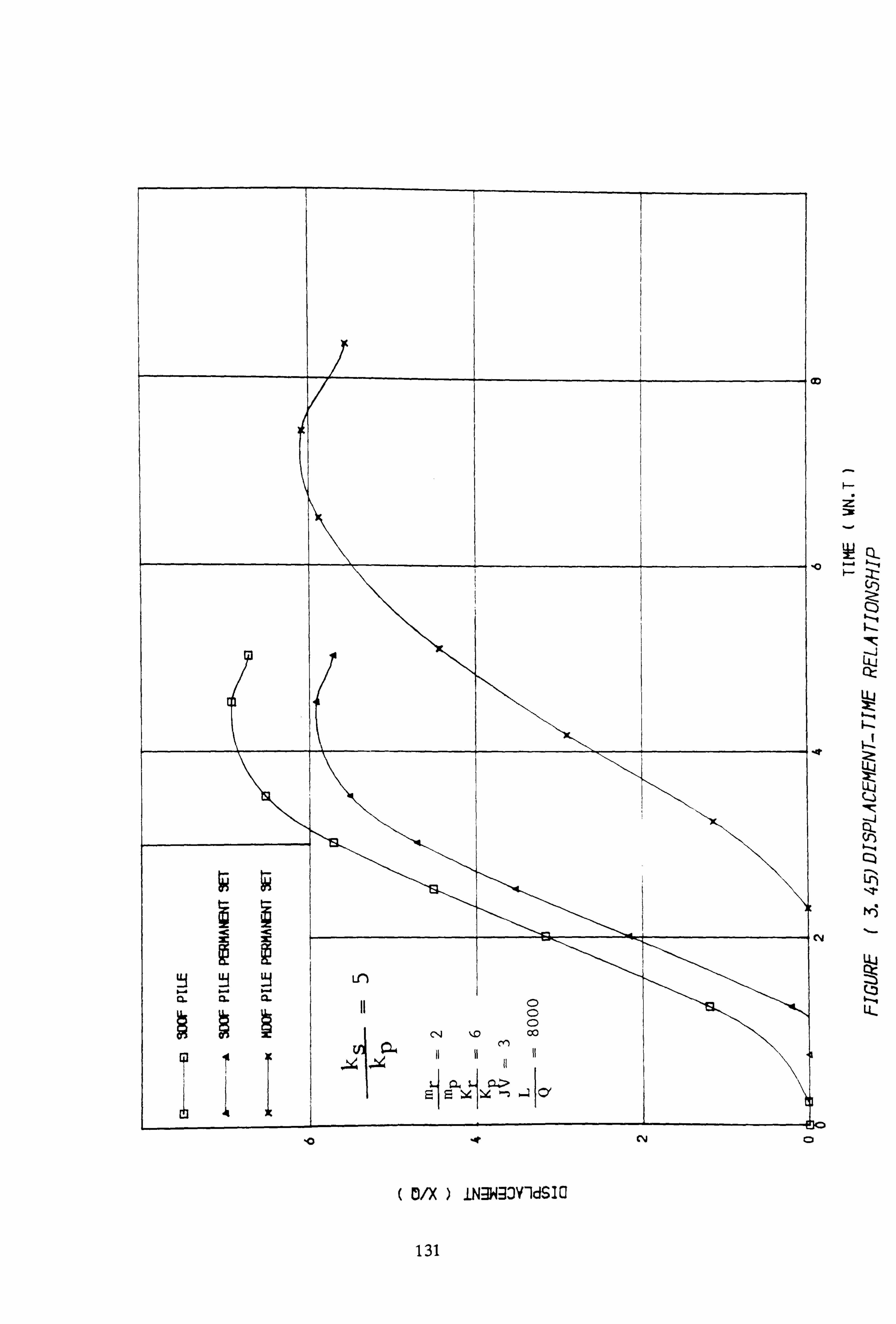
Ul CD CD CD

1x- 1 rzi Exu -lý -2 v

F 10

( DIX ) iN3W33VldSIC

C%j

m

10

-At

, C-4

-Mo Cl

H-

()

li uJ QL-

I IL

131

if-) LLJ

LU

CL

V) U-)

CD

clý %lo 0 m 00

.jI CY

oo

10

( NW ) 13KAWVýi

132

(\I Cl

,0 :Z : DC

LLJ

N

(D

Qý 1-4

-j LLJ Or LQ ZZ

ii

"0

fr

LLJ

Ul Ui §§1

C14 11.0 0 0") V) (n 00

11 11 Ln

-At rn N

( OIX ) lN9W33V-ldISI0

0.

140

K)

. uo

a

S

LU 2c CL

LLJ c

LL

133

: 31C

LLJ Q Cr a? Z.

(NW) 3380--1 WV8

LIJ

134

cli Cl

-1 (1 . -. -

CD

00 cn T)

Lrl

( O/X ) iNgW; 13Y-ldSIC

Ln 6

ON

ýo

K)

L

I- S

ýHc Q- to

H

'-4

I-

I Lij

LL

135

LU 3:

Q- 1-9 Z-

LU

LLJ Q Q: CZ, LL Z,

Ln

LU

LL

(NW) -33dQ=l WY6

136

14t CY Cý

c -«C CD

CD

CL

1A1

i ýlo 00

cn l c -

Cl co e

( O/X ) INgW93VIdSIO

C%j

0.

%0

tc)

L a

I-.

I- S

z ". 0

x: (lý 9-4 k-i

-_j LIJ Qý

CZ1

Lki Q

a LL-

137

W LLJ En cn

LLJ uj

X: X: EL cr ct

LLJ uj IL

ui uj ui LLJ

-i -j -i -i M a: a: CL

U- U- U- U- C3 M C) C) C) C: ) mM X: X:

0 C)

00 C: ) cyl 00

11 11

fl- 10 Ln -ir K) (N

( D/X ) lNgW33Y-IdSIO WFt WIXYW

W)

N

-A (: ) C)

Z: 1. ý

Er) En -C

CL -C tn U-) Lu

C3

LLJ LLJ 2: cr- 0-ý

C3

cr

,. -I z LLJ

LLj

Cl- ILO

Ln

U-

138

ui LLJ V) cn

zz ui ui zz c<

ui uj Q- M-

LU LL

CL CL (a.

LL C)

00M0 00 LO Ln : co

X,

-t

W)

N

Lr) 04

( DIX ) INN93Y-IdSIO wnwixyw

C.. > -�

u M

-J --j LU

UJ -j LLJ z al Qr- V-"

V) N- z LLJ X: ---I 6-4 Q C3 M

--j LU , -a;

Z Uji lul

C)

Qj 0-4 LL-

139

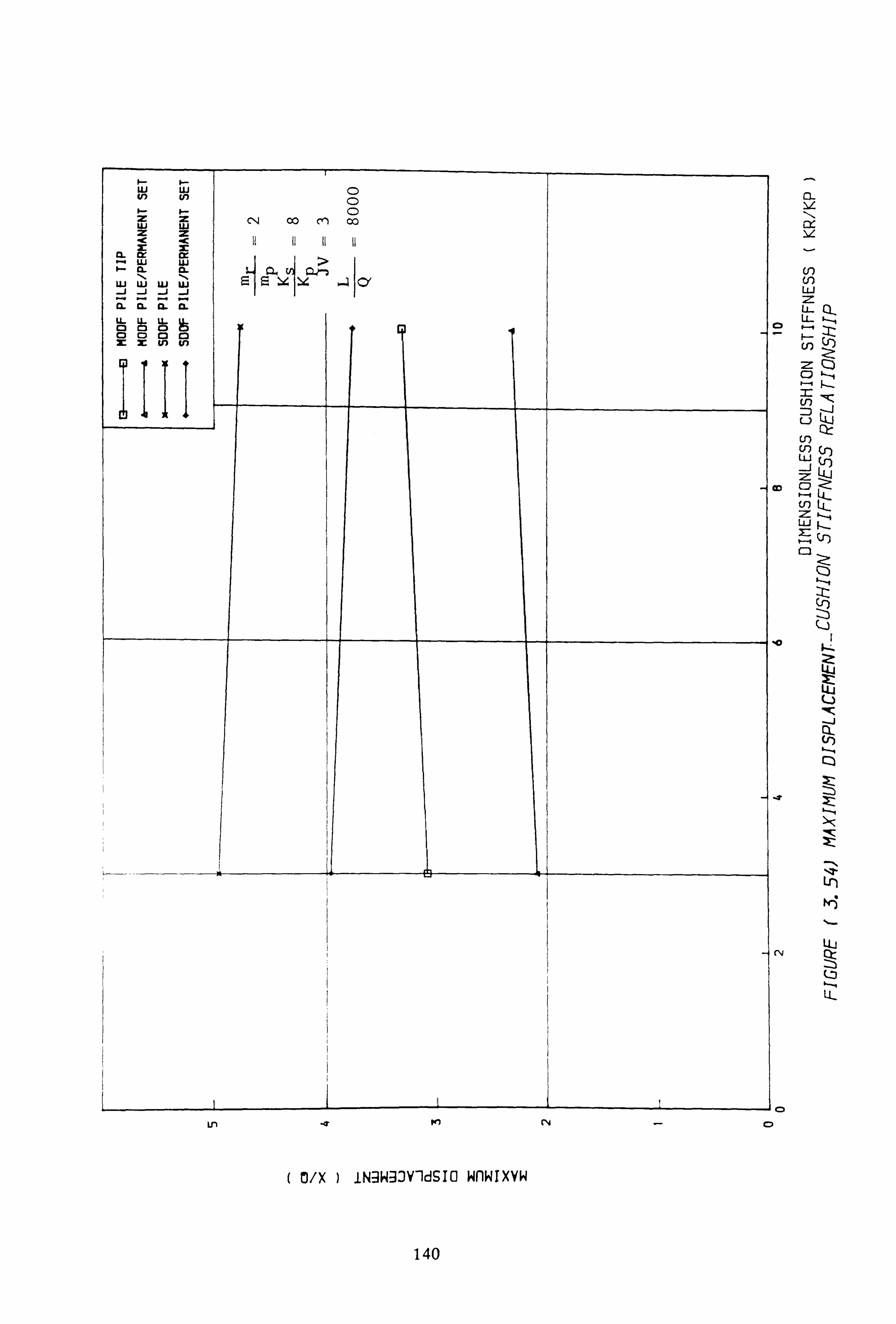
CL

LL-1

Cj

(n Z) w

Z: CD CD

b--f

tn :ZN. -4 LU

ýo 1

k.; - Z: L4i

CL (f)

4t

Ln

Lij 04 Ct

Z: ý

Q3

Cl

( O/X ) IN3W3: )V"ldSIO wnwixyw

140

Ln -4 ftl C)

0

S

ul ul ui Z n, U- LL

Ul

c2 tn Ul

(n w j Z

CD Ul Z ui Z u-- 0-4 LL

lIllz Z

U-j

Q3

Cý

( O/X ) INýiWgOV-ldSIO wnw i xvw

141

10 -r r. 4 CD

uj LU

Ui z

LLJ z

fr Lij

uj Uj

cr uj

LIJ uj

CL 0-

6 U-

0 C3 C3 2: X:

CL Cl-

661 00 C3 01 cn tn m

co

( D/X )

ýc -e

jNlý]DV-ýdSIC wnwixvw

rlj

z LLJ

_j UJ -j

Lu

-j "l< Z

m -_j

P" W

V)

z

uj

:1 RZ L-j

Cl CD

N-

LLJ

C) C-3

LL

0 0

142

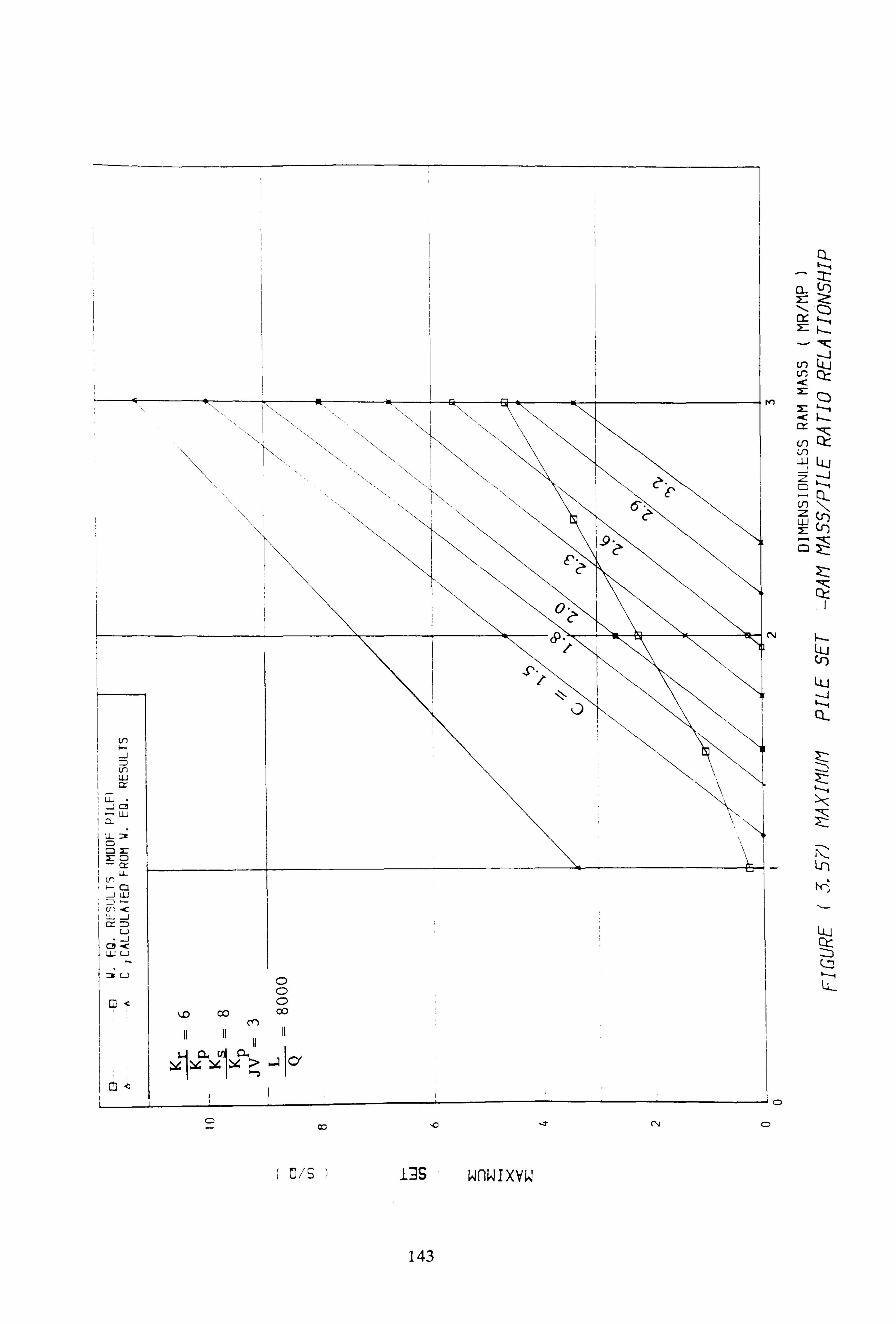
Q- 6--4 Z

a- Cr)

cr-

LO C: )

ul Ln LLJ

Cl- Ln z LLJ

in Zý Z:

LLJ (ri LLJ

Cl-

: L- Zj '-4

Ln

LU Q: 1-

LL-

CD

( C/S ) AS wnwixvw

143

Cl cc

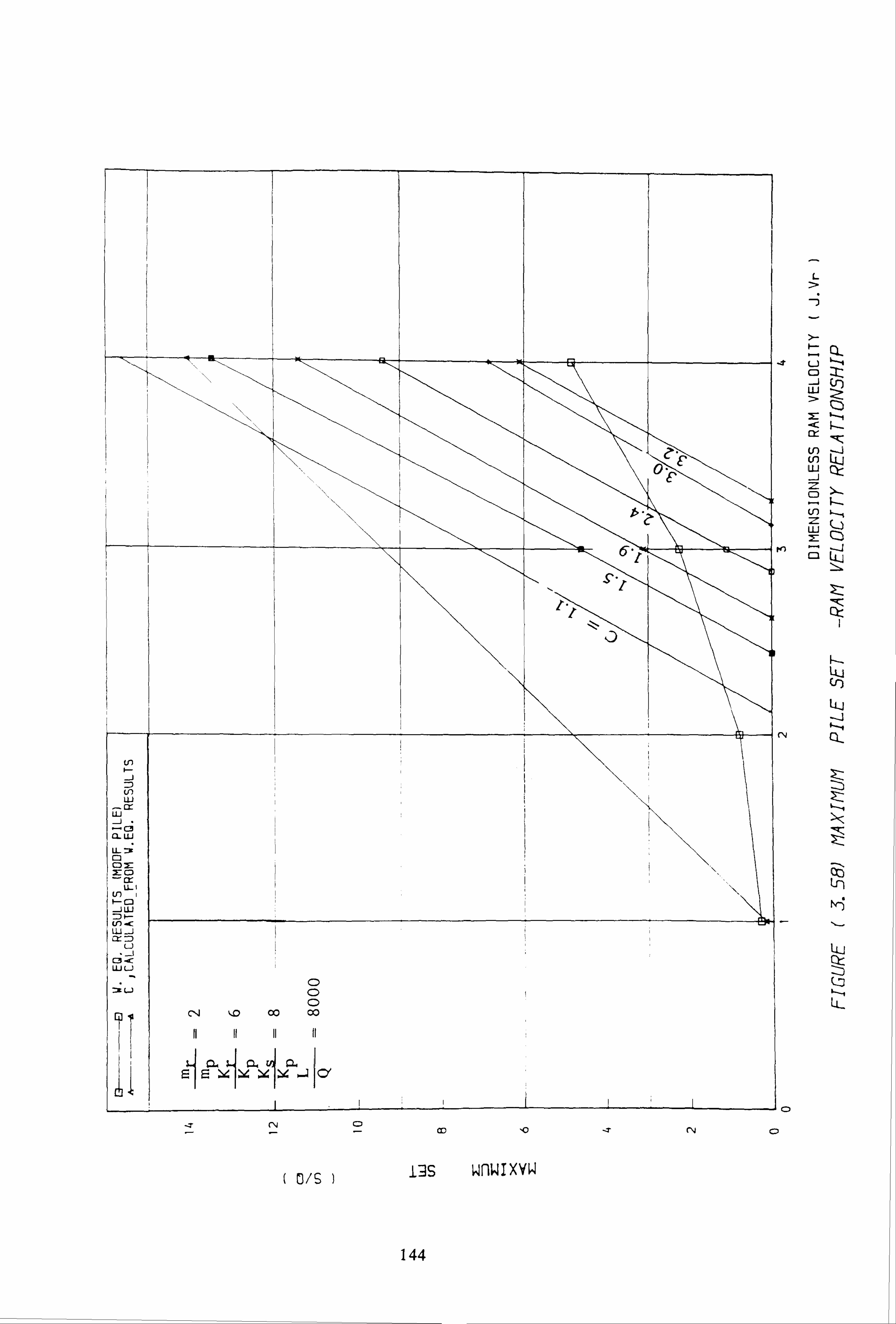
Ul uj

Lli ý ; Cý Q. LLJ

LL Cl C3 X:

C: ) cr LL U') ý- C3

-j uj

U') -C

U

C3 LLJ L. )

C: ) 0 0

C14 ý. o 00 00

0- i

E Eý4uý41 ce

-7 (N C) cc -T

( 0/6 ) As wnwixvw

L

-:

-T

W)

rlj

U

q

zt

cr- l< V) _-_j Ln LLj uj C)ý

C: ) Lo LU M: Cý

- -j ca

Or I

LLJ LO

Zý Zi

Ln

Cý LL-

144

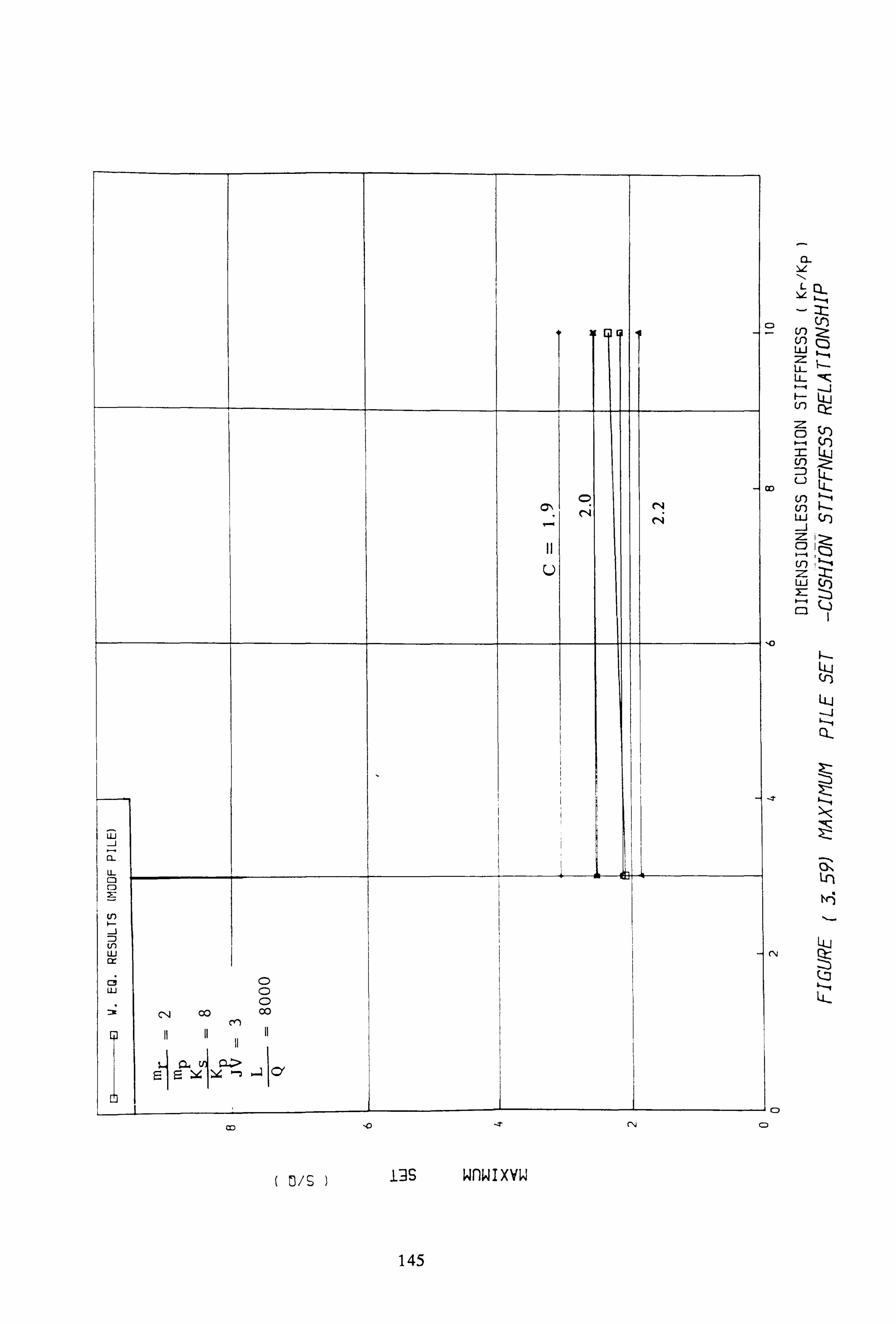
CD r9

CL U- CD

Ln LU

CD CD CD OD cli 00 cy)

co

145

--T

wnw i xvw

r--j

Co

10

--t

a-

L

LO Cr) LLJ LL- LL- Im<

:z o

LL,

u

Lu

Lli z ::: ) 0-ý Q

Cl I

LLJ (o

--l ON Ln

LLJ

LL-

-i CD CD

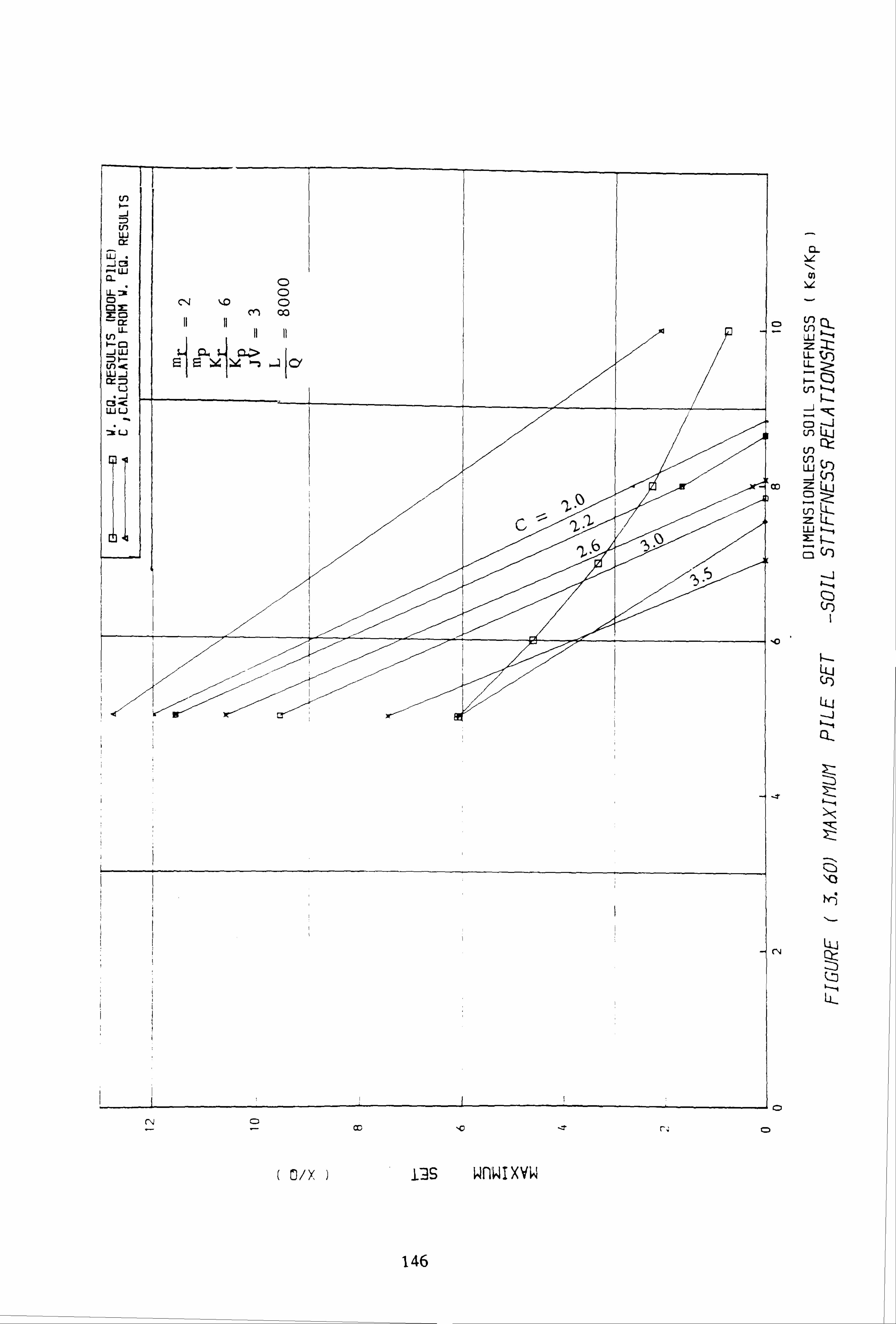
0,

CD V) CL LLI

Z: I-- Li- Ll-

V)

o Ln L4

LO Qr-

V) Lu -1 co z LIJ C: ) Ln uj X: ý-- cn

Cr) I

-0 .

LLJ

U) LLJ

-_j

\0

C4 Ll-j Qr

0

( O/X ) As wn, wixyw

146

C\j C) cl) C)

......... .

:: D V) LU cr

ci LU

rL LL nt CD

CD cc LL

Lo ý- CD

-1 LLJ

LO -<

u C3 Ic LU

00

'C - CD CC)

( C/S )i --ý S wnw i xyw

147

C) C) cl

0

Cý 1=1 LLJ

-i

LIJ

--i cl. Ln Ln

C) U-) z

C=) ui C) C) X: Q co cm -j

LLJ

I-- LL,

Cri C) CD No

CL

z CD Cl C)

LIJ Cl Cr CD CD N

C\j

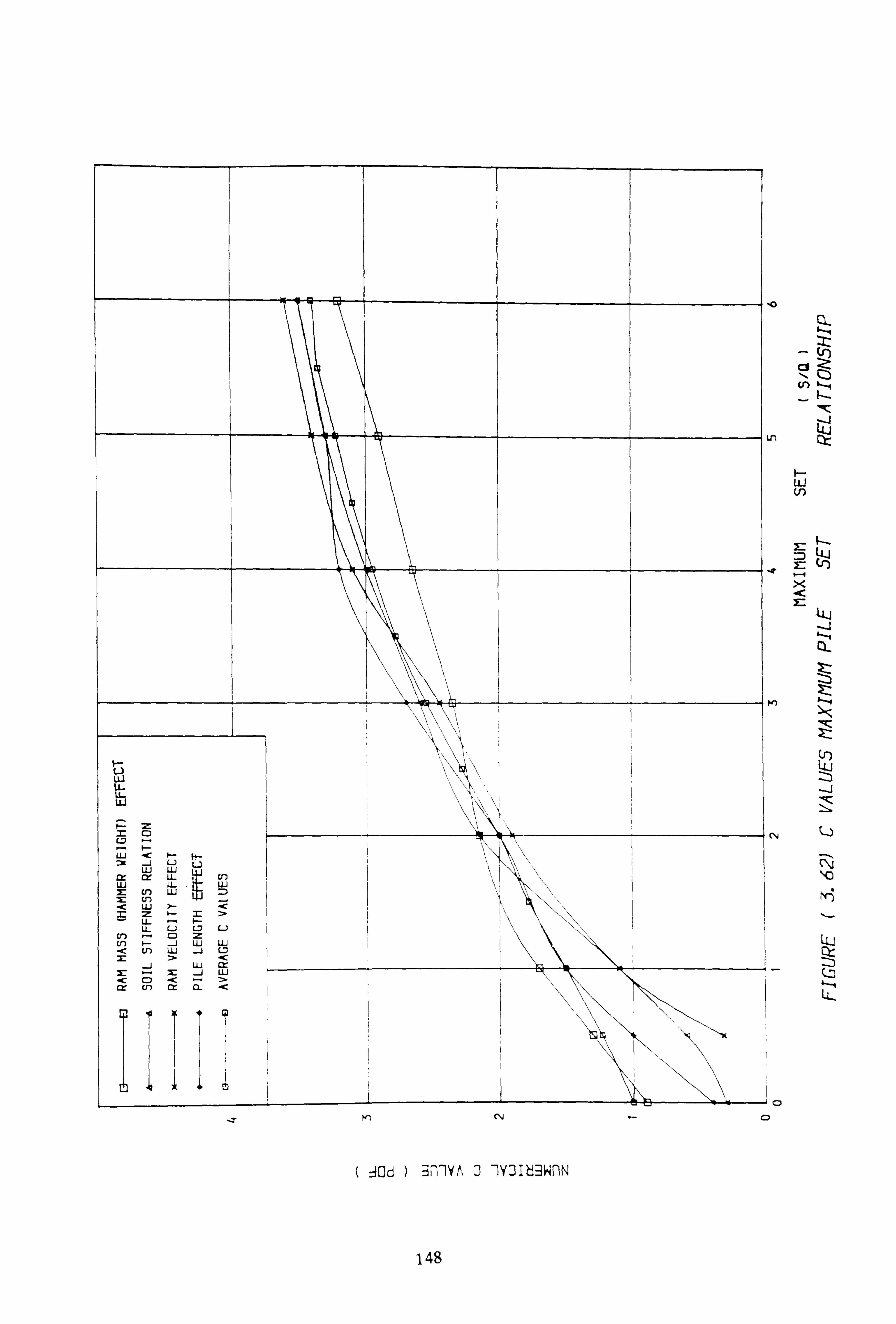
LLJ -C uj uj

= (x LL en uj Li- ui M: En LIJ X: En AC LLJ >- -C

N

U- L-) L-3 L. ) cr) CD z U. ) -j LLJ LLJ

En U.; -j L-) >. <I

\\',

- -i ui =I X: ý; X: -i LLJ -C . 1c cr to CX fa-

1 ýiýý 11 cl I-IW

--T K) CN

ý : Aod ) ýmyt, 3 7ui6ýiwnN

10 CL

cl Z:

I. -i Ln

Lw- Qý

ui (1)

= 1--

:3 14.1

Z: (ri

LL-

-. A C)

CD

148

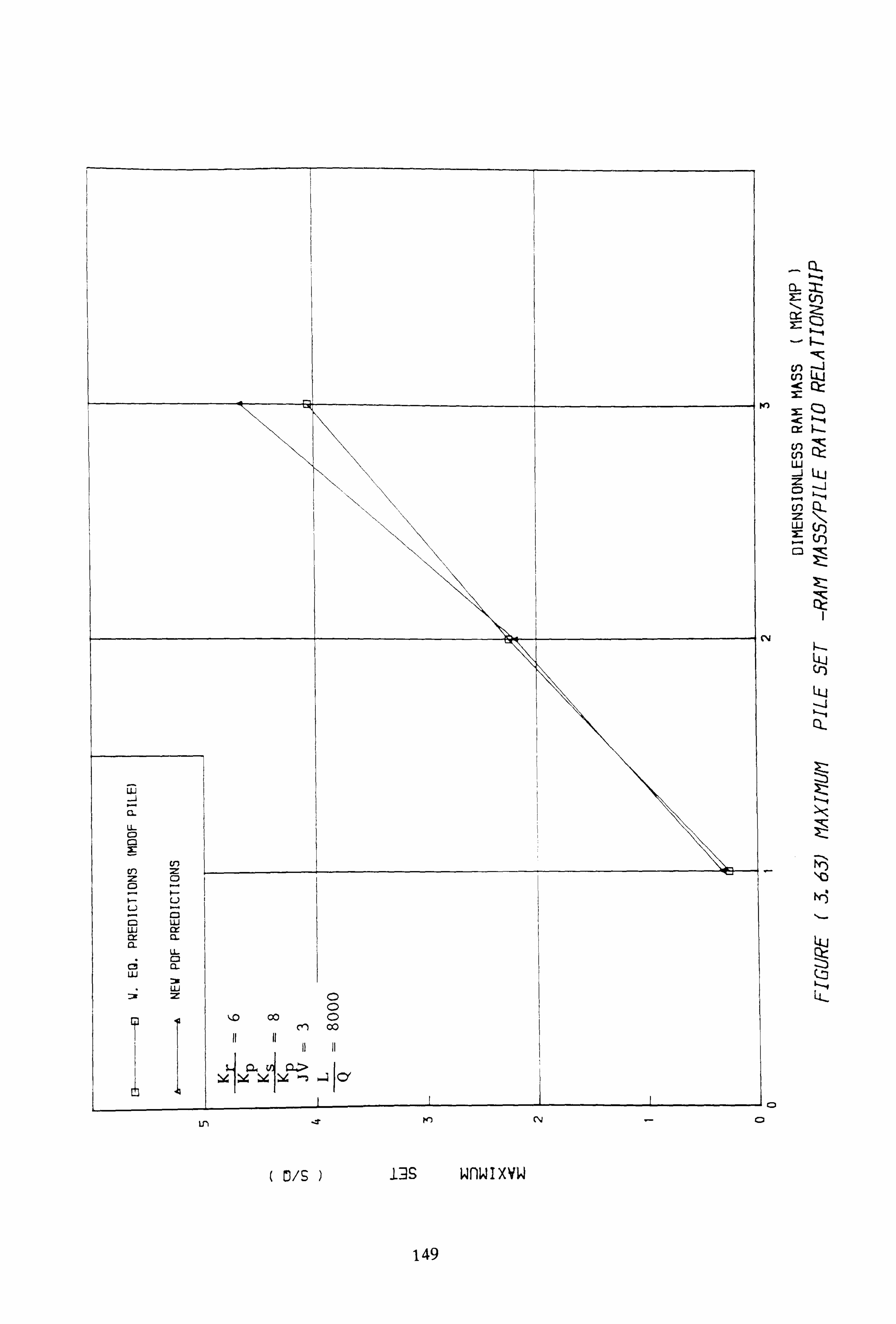
CL

U- CD C3

I= uj uj cr CL CL

LL C3

ui

Ll J C 0

00 CD CY) 00

11 11 1

1

0.91> i

CY

Lr) . -T

( O/S )

pe)

ils wnwixyw

149

0

N

CD

Q

Z: ('r) , --, Z.

En LLJ

cr) LU -j z C: ) Lo LU 2: 0ý 1: 3 ýý

k- LQ cri LQ

CL

Z77

i; ý

LLJ

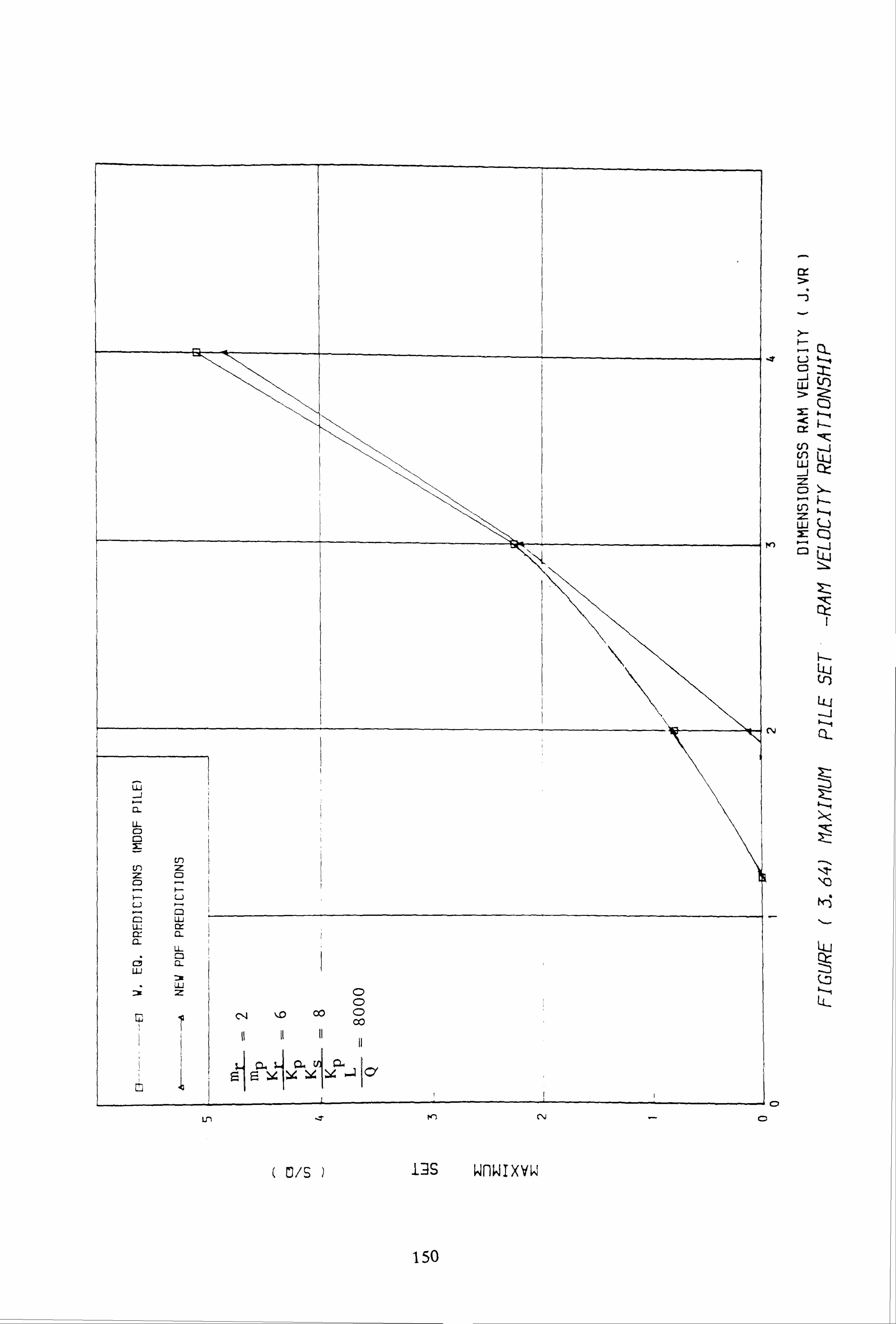
CD

U') z CD CD

L) L)

U-j LL

C; a- LU

LLJ

z C)

00 C) 00

Lr) ýT M-) C"i

( C/S ) ills wnwixvw

UJ

LLj LLJ 5ý I z c) LO :z 1-4 uj Q X: Q

LU (n

N Q-

Z:

fr

LL, ? 5l 1-4 LL

-. i CD

CD

150

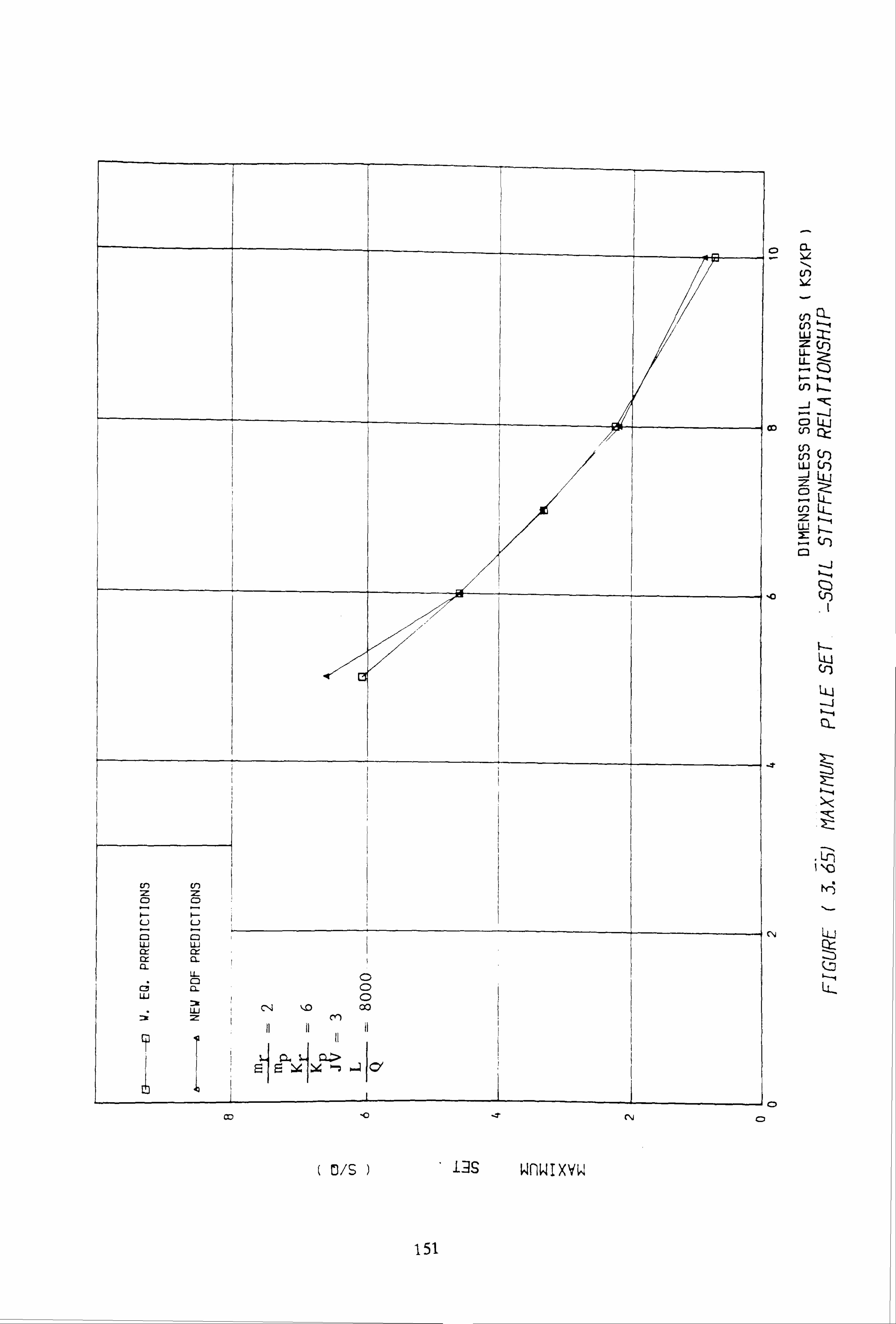
CL

cn

to (f) LU Z U- U-

-. J CD LLJ GD u-) Qz

u-) Co (0

U. i (r) i

Z 44 C: ) (n L, Z LU Z:

LU (f)

LLJ

CL

3z

- Ln 1%c

LLJ

LL-

C)

( [3/6 )ý 1'ýs wnw i xv ýi

15l

co Cl

( O/S ) i-ýs wnw i xvw

0 CD C)

-J

U) C) z C) uj

-j UJ CL

Lo V) U. 1 -j cl: z C: )

LO z Q'I

CD Uj CD co C3

LU

CL

I

LL,

10 LU -i 11-4 QL

ZZ

CD -. T Zý

Lu

1-1 Lk-

152

CC) 10 CNJ CD 0

ei = I--, ý14

LJ

aý LU

U. i Ci = )--4 C: ) ; -_ c2 ý9 V --J or: CD :X

ý. -1

-J

\0

LQ

19S LL-

0

( 8/)('S ) ils giid wnwixvw

153

Ln C)

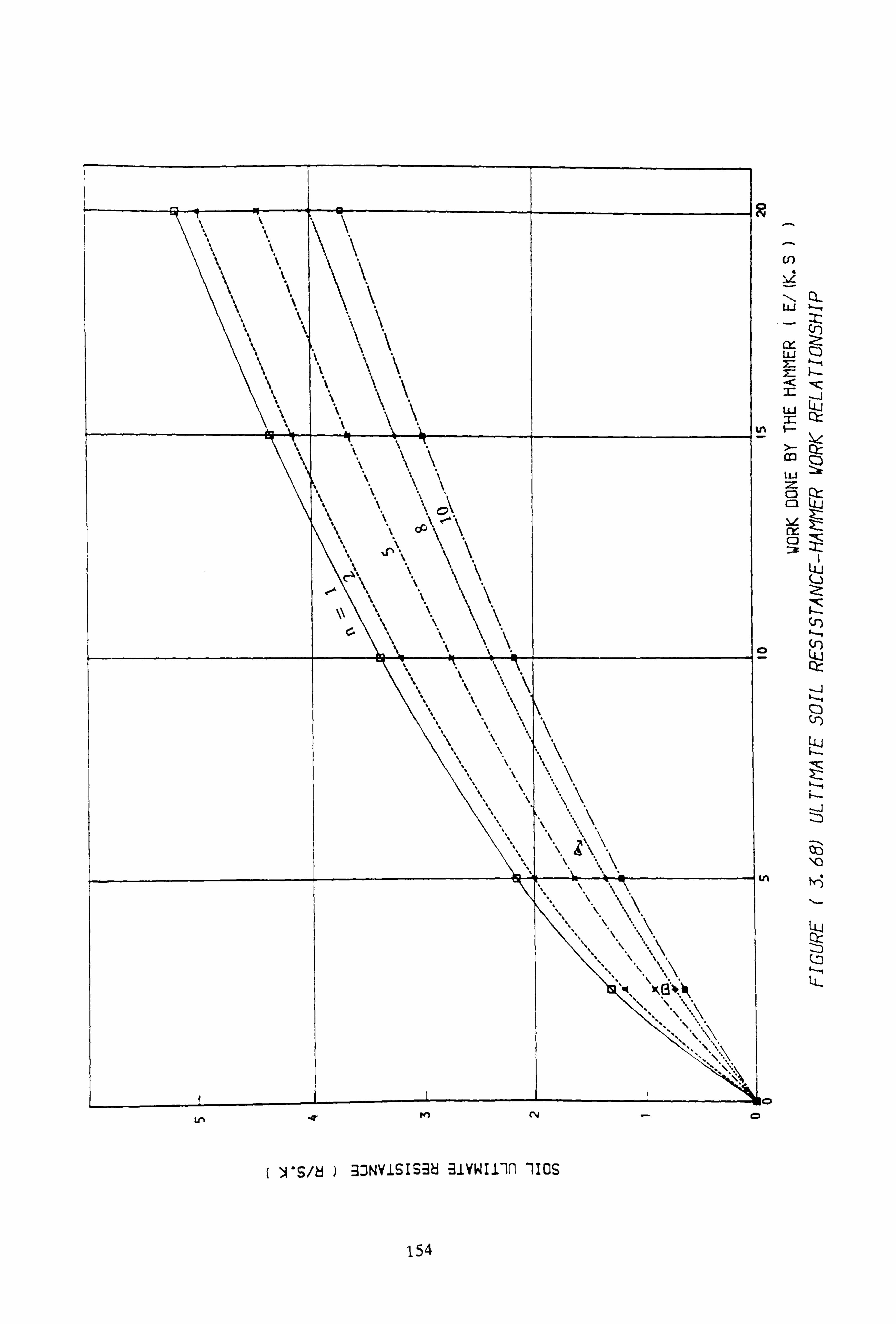
CAN

%1

ý%

Lr) . 4r W) CY

( )rS/8 ) 30NYiSIS-3? J 31YWIi7n iics

154

u-I

CL

Uj

<

Lij LU

>- Cl:

CD Q)

w : ýJk

C: ) Qr- cl lz ry C)

LLJ

Qr-

--l 00 NO

Ln

LIJ

rj

C -J

It i 00.1 ol I '".

C C

C C

C C U

C

? -t

N

NW "81 3ONYiSIS3H "110S

Q- 6-4

Zt

LLj

LU (n Lu

LLJ cl-

cn

LLJ

cr

LL,

,, a I- LLJ 2s

CV

-i C)

Cp

155

10

Ct-

C C

( (

( C

NW d 130NYISISIH 31Mrin imý

_I: C-0

LU CY

LLI to

LLJ

Cl

ILO 1: 7<

LLJ

LLJ Ot

-i 4

cr)

10

LU

ýi Qj I-M

C%j Ll-

Cl

156

%0 Li I

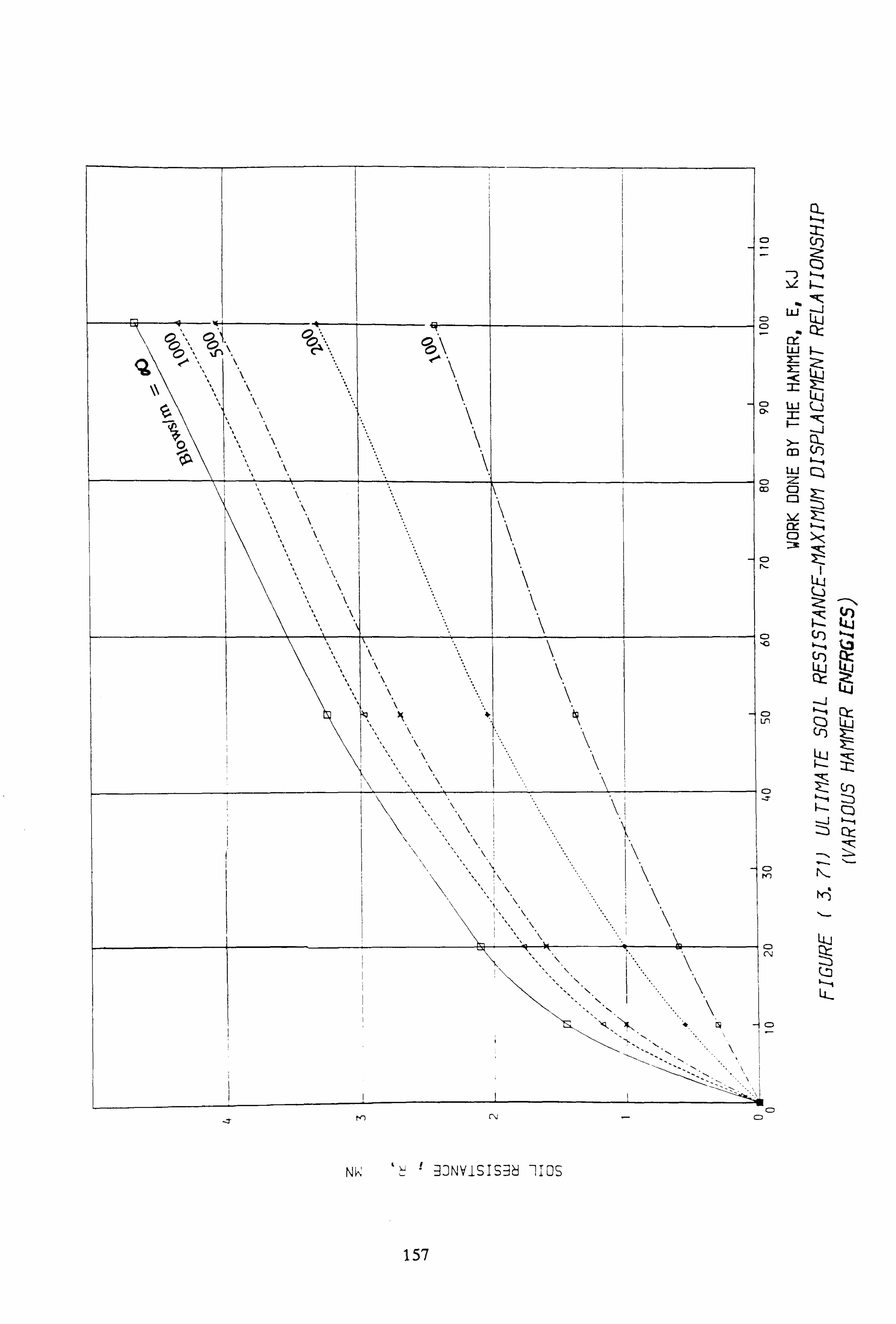
C

\

0-1 0ý \. W. 1.1.

O'l

Eq. 00

\ 1

l

-: r r4') cllý

t

ICS Nýý ýI ý3NViSISýý -11

Q-

UJ LLJ

LLJ

LU

m Cr) uj C: 2 C3

V-

C: )

LU QE

LL

C: )

LQ

L-)

157

C

C

/',

I,

T--q CD r--i cn , I-

r- ý- ýQ

C: ) CD

NW ý3NV ISIS ý? ý 71-ý ýiyW 11-7

LIT

Ln LLJ

V) LO ui I-

Ln LLJ Lij -i cr u U- tn m

LL; i LL :z

L. n C)

(. 0 Zt

Ln

Lr)

LLJ CL Ul)

--5 x

LU cr

LL-

ý CD

158

i- z LLJ

LLJ L) "C -i C2-

M

LLJ

LU -i a-

: 1ý (r) Z:

LLJ

701

LLJ

( -1 ) 9-Ild NO OYO-1 -IYN8ýiXý

LL,

159

r4 -4

CHAPTER 4

THE FINTTE ELEMENT MODEL

4.1 INTRODUCTION

4.2 THEORETICAL FORMULATION

4.2.1 Introduction

4.2.2 Governing Equations

4.3 CONSTITUTIVE LAWS

4.3.1 Introduction

4.3.2 Yield Criteria

4.3.3 The Critical State Model

4.3.4 Conclusion

4.4 SPATIAL DISCRETISATION

4.4.1 Introduction

4.4.2 Geometric Modelling

4.4.3 Transmitting Boundaries

4.4.4 Interface Elements

4.5 TIME INTEGRATION SCHEMES

4.5.1 Introduction

4.5.2 Explicit Integration Schemes

4.5.3 Implicit Integration Schemes

4.5.4 Implicit-Explicit Integration Schemes

4.5.5 Conclusion

4.6 CONCLUSION

CHAPTER 4

THE FINITE ELEMENT MODEL

4.1 INTRODUCTION

The finite element method (Zienkiewicz, 1971) is too cumbersome to be

attractive for routine pile driving analyses since computational costs are typically

two or three orders of magnitude greater than for the wave equation analysis. Its

main role therefore lies in providing accurate results using real soil properties.

In this Chapter, the essential concepts of the finite element model of

analysis for dynamic problems are outlined. Tensor notation is employed for

convenience in the development of the numerical algorithm from, the governing differential equations of motion.

Clearly, it is important to incorporate realistic soil models in the numerical

study and to that end, a number of alternatives, including a critical state model

are considered. However, since soil failure during driving takes place very quickly,

i. e. under undrained conditions, total stress analysis offers considerable advantages

and this approach is favoured in the sequel.

Spatial discretisation, energy absorbing boundaries and interface elements are

treated in depth. Further, convolution in the time domain, by various time

marching schemes (both explicit and implicit) is examined and the attributes of

the alternative formulations are discussed.

4.2 THEORETICAL FORMULATION

4.2.1 Introduction

The finite element method (Zienkiewicz, 1977) is, as is well known, a very

160

powerful and general solution technique. Algorithms for solution of non-linear

dynamics problems were published quite early (Seed and ldriss, 1970; Lysmer et al,

1975; Angelides and Roesset, 1980) but significant problems remain in regard to

practical implementation of the method, viz spurious energy reflections at element interfaces (Holmes and Belytschko, 1976) and at curtailed (infinite) boundaries

(Lysmer and Kuhlemeyer, 1969; Chow and Smith, 1981), suppression of higher

modes within elements (Celep and Bazant, 1983 ) and high computational costs. These difficulties are discussed in the sequel but first the derivations of the

governing differential equations and the basic formulation of the numerical

algorithm are given for completeness.

4.2.2 Governing Equations

In the linear theory of elasticity, the strains can be written in terms of displacements as:

Eii= 1

(ui, j + uj, i)

2

where,

ui is the i-th cartesian component of displacement,

ij are subscripts ranging from 1 to 3, and,

the comma, denotes differentiation with respect to the space variable, i. e.

ui, j= C)Ui/, Dxj.

The law of conservation of momentum states that the rate of change of

momentum is equal to the net force acting on the body, (Eringen and

Suhubi, 1974; Graff, 1975). For an infinitesimal element, this may be written as:

aij, j+bi = pui (4.2)

161

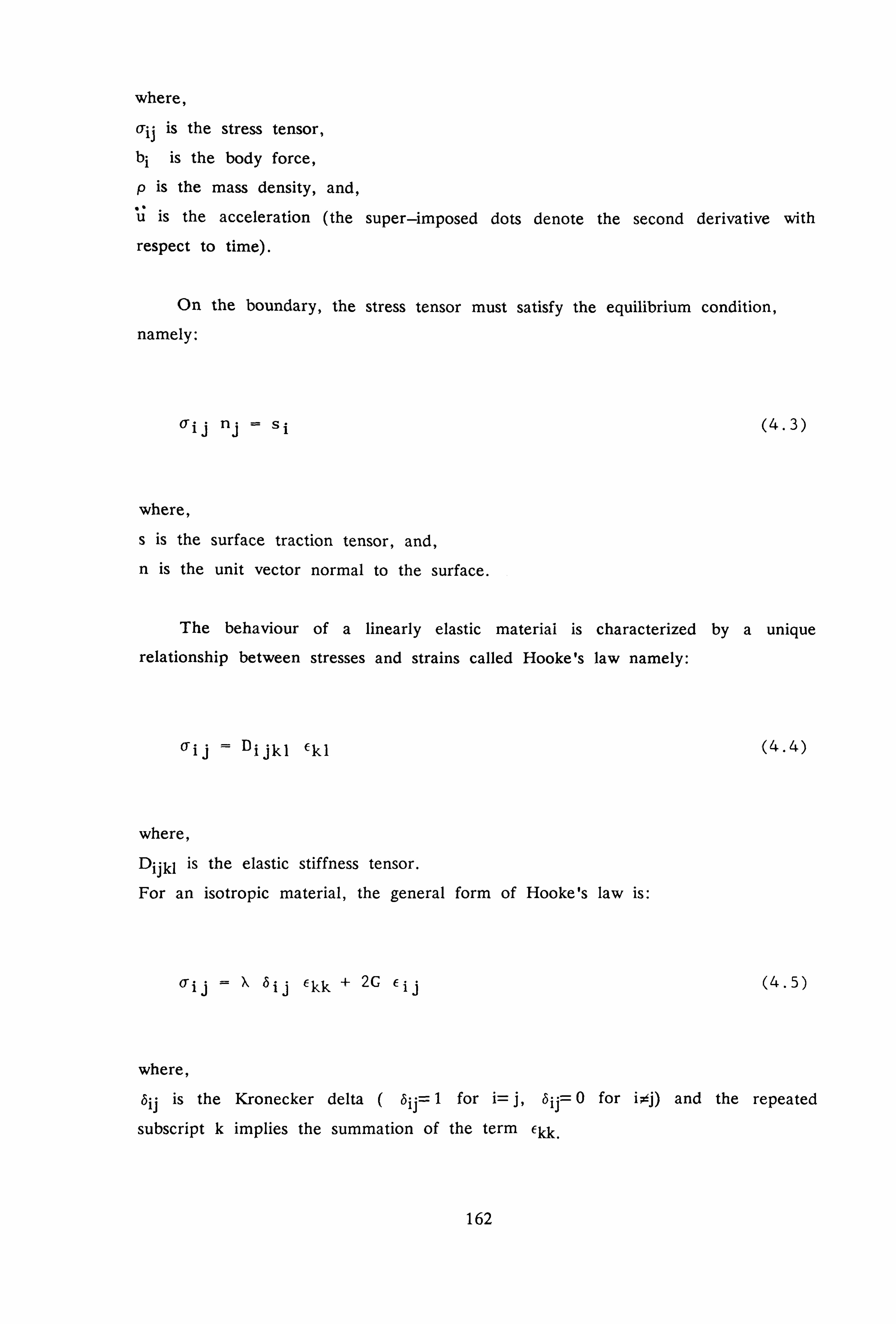
where,

o-ij is the stress tensor,

bi is the body force,

p is the mass density, and, "0 u is the acceleration (the super-imposed dots denote the second derivative with

respect to time).

On the boundary, the stress tensor must satisfy the equilibrium condition,

namely:

o-ij nj = si (4.3)

where,

s is the surface traction tensor, and,

n is the unit vector normal to the surface.

The behaviour of a linearly elastic material is characterized by a unique

relationship between stresses and strains called Hooke's law namely:

(Tij = Dijkl 'Ekl (4.4)

where,

Dijkl is the elastic stiffness tensor.

For an isotropic material, the general form of Hooke's law is:

O'l jý ý' 6ij 'E kk + 2G iEi j (4.5)

where,

bij is the Kronecker delta ( bij= 1 for i= j, bij= 0 for ip--Ij) and the repeated

subscript k implies the summation of the term Ekk.

162

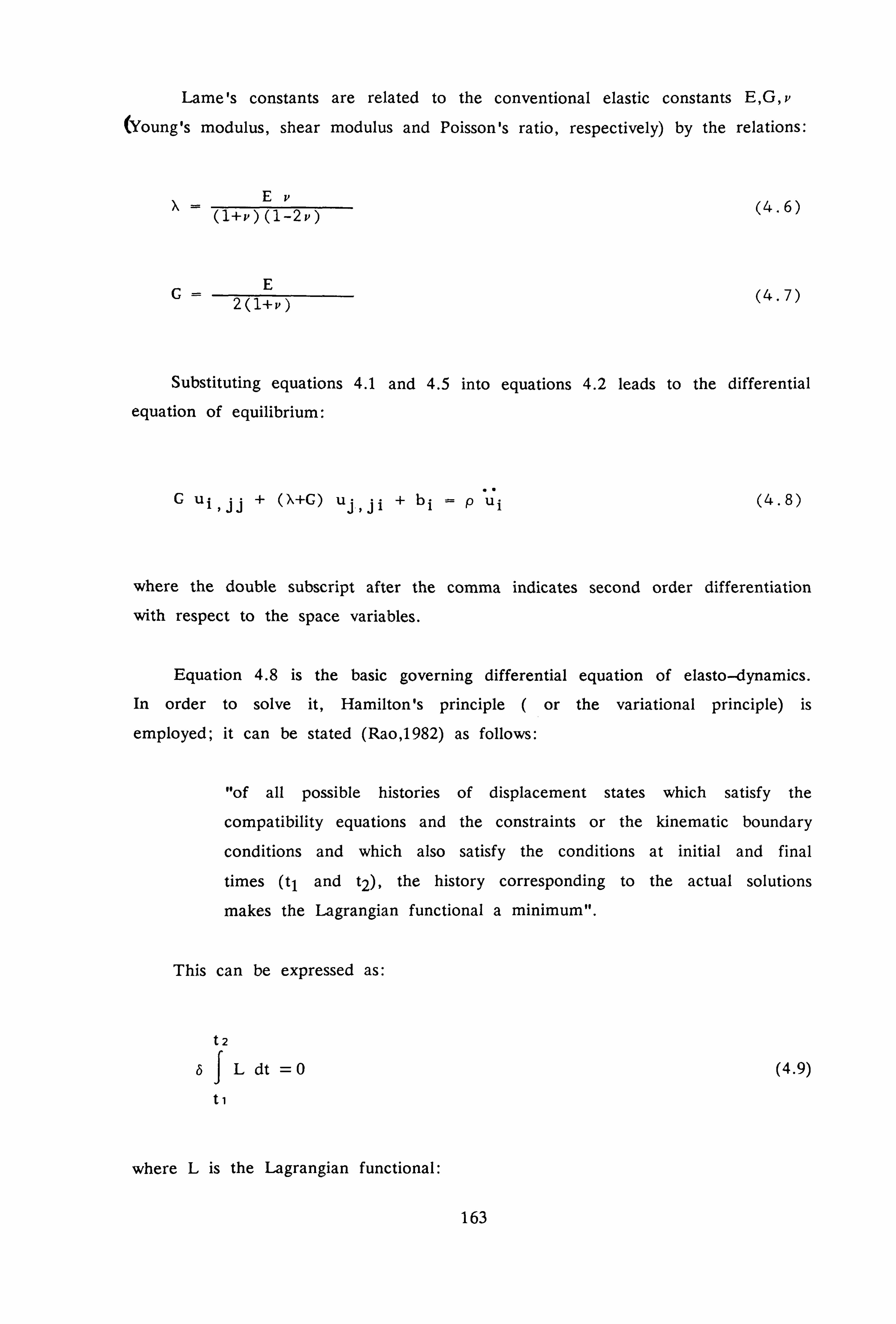
Lame's constants are related to the conventional elastic constants E, G, v (Young's modulus, shear modulus and Poisson's ratio, respectively) by the relations:

x=EP (4.6) (1+p)(1-2p)

E (4.7) 2(1+1, )

Substituting equations 4.1 and 4.5 into equations 4.2 leads to the differential

equation of equilibrium:

ui, jj + (X+C) uj, ji + bi p ui (4.8)

where the double subscript after the comma indicates second order differentiation

with respect to the space variables.

Equation 4.8 is the basic governing differential equation of elasto-dynamics. In order to solve it, Hamilton's principle ( or the variational principle) is

employed; it can be stated (Rao, 1982) as follows:

"of all possible histories of displacement states which satisfy the

compatibility equations and the constraints or the kinematic boundary

conditions and which also satisfy the conditions at initial and final

times (tj and t2), the history corresponding to the actual solutions

makes the Lagrangian functional a minimum".

This can be expressed as:

t2

6fL dt

ti

where L is the Lagrangian functional:

(4.9)

163

rl

and, K is the kinetic energy of the body,

U is its strain energy, and,

rl is the potential energy of the external forces acting on the body.

(4.10)

Now let the volume of the body under consideration be V, and its surface

area be S. Applying the principle of virtual work ( the principle states that at

equilibrium, for any compatible, small virtual displacements imposed on a body,

the total internal virtual work is equal to the total external virtual work; Bathe

and Wilson, 1976) and using the methods of variational calculus, Hamilton

derived a general formulation of the equations of mechanics that describes the

motion of the system with finite or infinite degrees of freedom. The mathematical

statement of Hamilton's principle (Rao, 1982) is:

t2

f(L+W) dt

ti

where W is the total external work, except that done by inertial forces,

and,

6w I

Si bui dS +f bi bui dV (4.12)

sv

where,

6W is the virtual work done, and,

6u is the virtual displacement.

Equation 4.11 can also be expressed in terms of kinetic energies as follows:

t2

f( Fl + W ) dt (4.13)

164

where,

t2t2

c) K K dt f

dt f

aui 6ui dV (4.14)

ti ti v

and,

t2t2

rl dt dt -; -f. j6cij dV (4.15)

f

ti ti v

also we have,

6ui at (bui) (4.16)

and,

1 (4.17) (6ui), j + (6uj), i

I

By applying the divergence theorem;

f o-ij

ýi, j dV

f o7i j

ýi nj dS (4.18)

vs

and assuming that

Dfl fi

)K and, o7ij nj = Si

C)Eij 'Dui

165

then, equation 4.13 (after substitution and simplifications) becomes

t2t2 1

dt 11

(o-ij, j -p U*i + bi ) bui dV 1- 11

fi bul dv ]=o

v

This represents the integral form of the equation of elasto -dynamics. Equation 4.19 can also be written by dropping the tensor notation as:

t2t2

1 dt

ff 07 -pU+ b) bu dV bu dV

I=0 (4.20)

ti vv ti

where, b is the internal body force vector, which can also be defined in terms of the damping parameter (in the form b= c ý, where c is the damping coefficient)

and,

u, U and qu* are the displacement, velocity and acceleration vectors, respectively Following the usual finite element procedures, the displacements, velocities

and accelerations can be expressed in terms of the associated (element) nodal

values as:

Nx (4.21)

Ný (4.22)

N *X (4.23)

where, the summation is carried over each element node,

x, i and i are the vectors of nodal displacements, velocities and accelerations,

respectively, and

N is the element shape function.

By applying the principle of virtual work, equation 4.20 can be written for

166

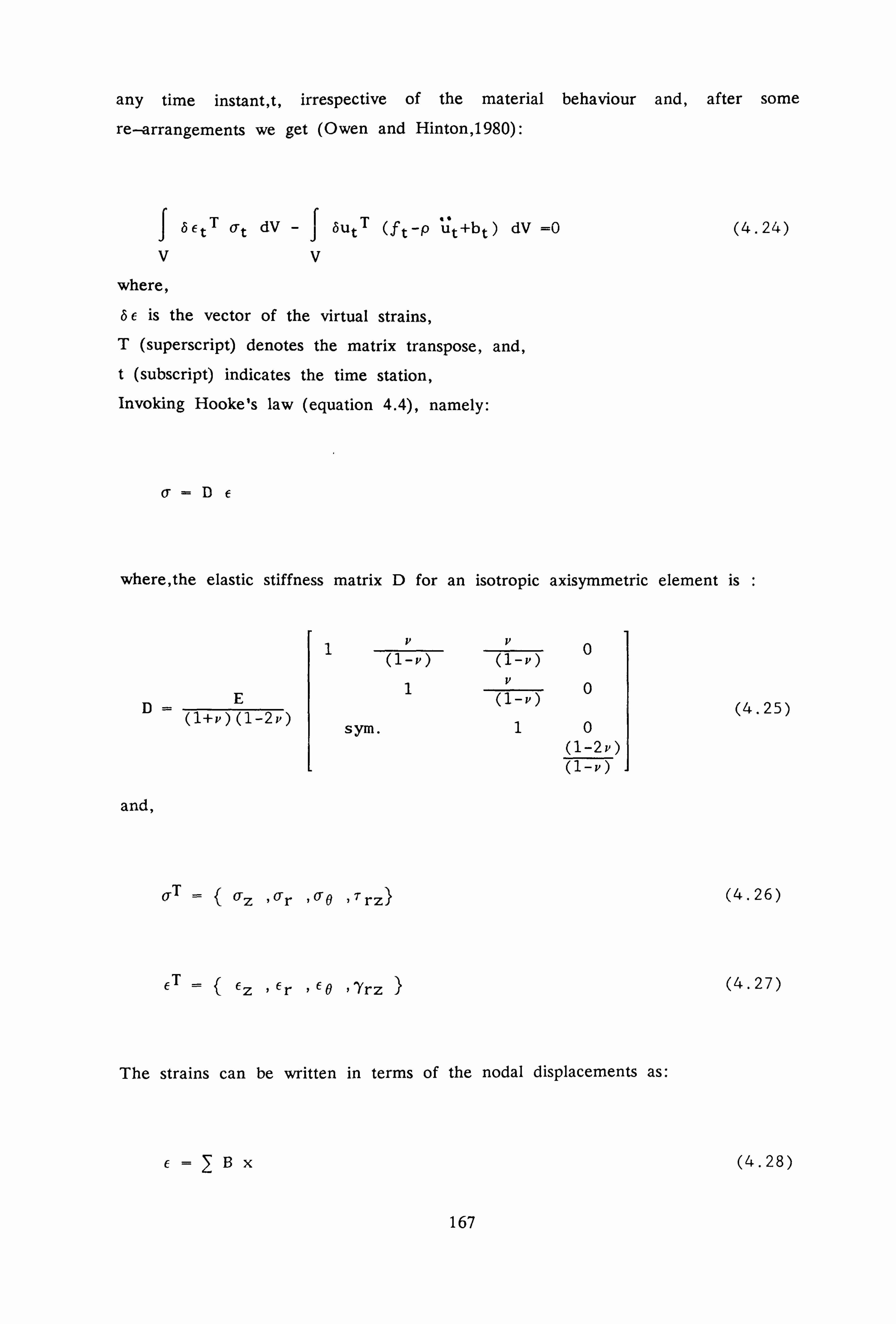
any time instant, t, irrespective of the material behaviour and, after some

re-arrangements we get (Owen and Hinton, 1980):

f betT o't dV -f 6utT (ft-p ut+bt) dV =0

VV

where,

6c is the vector of the virtual strains, T (superscript) denotes the matrix transpose, and, t (subscript) indicates the time station, Invoking Hooke's law (equation 4.4), namely:

o7 =

(4.24)

where, the elastic stiffness matrix D for an isotropic axisymmetric element is :

E (I+v)(1-2v)

and,

sym.

O, T =( O-Z O-r aO "rz)

6T =( Iz Ir 60 Yrz )

The strains can be written in terms of the nodal displacements as:

f=ý

(4.25)

(4.26)

(4.27)

(4.28)

167

where B is the strain-displacement matrix. For the isotropic axisymmetric

element, it is defined as follows:

B=

aN - 0 ýT r

aN 0

az N

0 r

aN C) N az

(4.29)

By substituting equations 4.20,4.21,4.22 and 4.23 into equation 4.24 we get :

1 BT DB öx x dV -1 NT f öx dV +1 NT pN öx *x* dV

vvv

f NT cN6xý dV

v

(4.30)

For a single finite element, equation 4.30 can be written in the form:

2 (4.31)

where, the summation is carried out over each element node,

M is called the mass matrix, where,

m=f NT pN dV (4.32)

v

C is called the damping matrix, where,

168

C=f NT cN dV (4.33)

V

and K is called the element stiffness matrix, where,

K=f BT DB dV (4.34)

v

Assembly of equations 4.31 for each element of the body and invoking the

compatibility and equilibrium conditions of the nodes, yields by superposition the

global system equations:

MX+C+K (4.35)

where, M CK and F are the global mass, damping and stiffness matrices,

respectively, and F is the forcing matrix.

The solution of these equations can be achieved by integrating them in the

time domain by means of the methods discussed later in this Chapter.

4.3 CONSTITUTIVE LAWS

4.3.1 Introduction

Realistic constitutive laws are essential if reliable results are to be obtained

using the finite element method. However, advances in numerical analysis have

far exceeded knowledge of soil behaviour, Hill (1950), Desai and Siriwardane

(1984). Thus results from sophisticated numerical analyses should be treated with

some caution.

169

The simplest constitutive model assumes isotropic linear elasticity. However,

this model is only useful at small strain levels and it is necessary to use

elasto-plastic flow theory to describe soil be haviour at strain levels of interest.

Due to the fact that pile driving involves impact forces of short duration,

undrained behaviour can be assumed to occur. Consequently, total stress analyses

and simple elastic-perfectly plastic soil models can be used for convenience. Some

of these models are discussed in what follows.

4.3.2 Yield Criteria

It is postulated that flow occurs within a material when the current stress

state satisfies certain energy criteria or reaches specific critical values. The

one-dimensional concept of a yield stress, from the simple tension test, Fig. 4.1

and Fig. 4.2, leads naturally to the idea of the yield " surface", Fig. 4.3, in

(principal) stress space. The yield criterion is then conveniently defin ed by a yield

function F as (Davies, 1979 and Desai and Siriwardane, 1984):

F(o-ij) =

where,

F=0 implies that the material is on the yield surface, i. e.

plastic flow takes place,

F<0 implies that the material lies within the elastic domain

i. e. the material deforms elastically,

0 is inadmissible.

(4.36)

in general, plasticity theory can be developed to allow for expansion (work

hardening, strain hardening), contraction (work softening, strain softening) and

170

translation (kinematic hardening) of the yield surface depending on the type of

the flow rules and hardening parameters used.

Since, for isotropic materials, the yield function must be invariant with

respect to all reference frames, it must be expressed in terms of the invariants of

the stress tensor, i. e.

F(11,12,13) ý0 (4.37)

where 11 j 2,13 are the first, second and third invariants of the stress tensor, given

by :

Il = 0-! i

12= 1/2 (0-ii orjj - 0-ij aij)

13 = 1/3 (O'ij 07jk 010

(4.38)

In metal plasticity, it is assumed that yielding is unaffected by the hydrostatic

stress ( 1/3 o-ii ) and, accordingly, the yield function is usually expressed in terms

of the invariants of the deviatoric stress tensor ( sij ) or :

F(J2 J3)

where,

(4.39)

171

Jl=O

J2ý1/2 sij sij

J3ý1/3 sij sjk ski

where the deviatoric stress tensor sij is defined as follows :

sij = o-ij - 1/3 6ij 07kk

(4.40)

(4.41)

Many yield criteria have been proposed, of which the most well known are

those due to Tresca, Von Mises, Mohr-Coulomb and Drucker-Prager. Tresca's

criterion (the condition of constant maximum tangential stress) defines a hexahedral prism in principal stress space and implies that the maximum shear

stress within the body can not not exceed a certain specific value. The attendant

mathematical difficulties of formulation in three dimensions (because of the

corners) has precluded its general use in theoretical analysis.

Von Mises criterion, which defines the circumscribed cylinder, is much more

amenable to theoretical development; it is simply a function of the second

deviatoric invariant:

F(J2) ý0 (4.42)

Since J2 corresponds precisely, up to a scalar factor, with the energy of the

elastic change of shape, the Von Mises criterion is some times called a distortional

energy criterion. This criterion was first proposed by Von Mises in 1913.

According to this theory, plastic yielding starts when the elastic strain energy due

to shearing reaches a critical value, when the following equation (in terms of

principal stresses) is satisfied:

172

( o'1 - or 2)2+( 0- 2- Or3 )2+( 073 - 071 )2= 2u y2 (4.43)

where uy is the yield stress (in uniaxial loading).

In principal stress space, the Von Mises yield criterion describes a cylindrical

surface, Fig. 4.4 , about the hydrostatic axis.

These two criteria were developed specifically for metals from observations of their behaviour. The behaviour of soils differs in many respects; in particular, the

yielding of soil is highly dependent on the hydrostatic component of effective

stress. Further, a realistic constitutive model for soils should be capable of taking into account features like dilatancy, sensitivity and strain hardening. Much research

effort has been developed to improve the predictive capacity of constitutive laws

for sands and clays. Important conference proceedings have been edited by Parry

(1972), Palmer(1973), Murayamo and Schofield (1977), Yong and Ko (1981),

Desai and Saxena (1981) and Desai and Gallagher (1983). The workshop chaired by Yong and Ko (1981) is especially interesting since many of the important

existing soil models were compared for their predictive ability. The general

conclusion was that a complicated, all-encompassing soil model is un-necessary (and undesirable on the grounds of cost) since simple models can often provide

equally useful results. Further, these models are generally, strictly speaking, valid

only for simple stress states. Thus, in view of the complicated state of stress

adjacent to the pile wall during driving and subsequent consolidation, utilization of

sophisticated material models offers little advantage.

4.3.3 The Critical State Model

The critical state model (Schofield and Wroth, 1968) is an elasto-plastic

constitutive law relating increments of strains to increments of effective stress.

When a loose soil sample is sheared, it passes through progressive states of

yielding before reaching a state of collapse. This means that the stress path

passes through several yield surfaces which results in (plastic) permanent

173

deformations. Yielding continues until the material reaches a critical void ratio,

after which the void ratio remains constant (i. e. no volume change occurs) during

subsequent deformation. This is called the critical void ratio and the failure

stress-volume condition of the soil is termed the critical state. However, when a

dense soil sample is sheared, the maximum shear resistance is developed during

dilation but as the critical void ratio is approached the shear resistance falls to

its critical state value.

Critical state models were originally developed by Roscoe's research group at

Cambridge University in the 1950's and 60's, (Schofield and Wroth, 1968) based

on conventional triaxial tests on consolidated reconstituted kaolin slurry. The

model is described in terms of the effective stress invariants (p and q) and the

specific volume V as defined below (Wood, 1984).

Mean normal effective stress

pý11 o- 1+ 0- 2+ o- 31 (4.44) 3

Deviatoric stress (q):

(0-1-0-2 ) 2+ (072-073 )2+ (07 3 -0-1

)2 ]l /2 (4.45)

Specific volume (V) :

(4.46)

where e is the void ratio.

Under conventional triaxial conditions at least two of the principal stresses

are equal resulting in some simplification. Further, by the principle of effective

stress, total and effective stresses are related via equations of the form

174

0-1 = Ol t-u etc. (4.47)

where u is the pore water pressure.

In the critical state theory, the consolidation and swelling lines are assumed to be straight in the (In p-V) plots, with slopes (X) and ( K), respectively, (Fig. 4.5)

which assume the role of material parameters in the critical state theory. These

lines can be described by the equations:

ro -x In p (4.48)

where r. is the specific volume at unit mean effective stress on the consolidation line, and,

Vý VM +K In p (4.49) Pm

where Vm is the specific volume on the consolidation line at a mean effective

stress of pm.

When the soil sample is sheared, it approaches the critical state line which is assumed to be parallel to the consolidation line in the V-p space

V=F-X In p (4.50)

where T' is the specific volume at unit pressure on the critical state line.

In terms of stress-invariants, the Mohr-Coulomb failure criterion can be

expressed in the form

p (4.51)

175

whereq for example, for triaxial test results the parameter M is given by the

equation:

6 sin cD (4.52) (3 - sin cD)

where (t is the angle of internal friction (at the critical state).

The value of M determines the slope of the critical state line in the p-q

plot, Fig. 4.6 , while r locates this line in the corresponding p-V plot shown in

Fig. 4.6. Although this line (curve) describes the failure state of the soil, detailed

observations from a comprehensive series of tests are necessary to establish the

shape of the yield surface. As noted earlier, this is a function of both the deviatoric stress q and the hydrostatic effective stress p. Schofield and Wroth

(1968) first proposed a yield surface described by the equation (in q-p space) :

q=Mp In PM (4.53) P

where pm is the past maximum mean effective stress which the soil has

suffered.

This gives rise to the idea of a state boundary surface in (q-p-V) space

given by the equation (Fig. 4.8):

q=(Xr+X-K-V-X1np] (4.54)

When the state of stress of the soil lies within this surface, the behaviour is

elastic (over-consolidated) while the behaviour on the surface is elasto-plastic; any

stress state outside this surface is inadmissible.

It is assumed that the under elastic conditions changes in the deviatoric

stress, q, do not cause changes in the void ratio and consequently the elastic

176

behaviour is constrained to a vertical "elastic wall", whose locus with the state

boundary surface defines the current yield criterion. Upon further consolidation, or

elasto-plastic loading the stress-state passes through successive adjacent yield

surfaces and their associated elastic walls (Fig. 4.9).

This model of soil behaviour which accommodates the phenomena of dilatancy, frictional failure and consolidation behaviour has been modified by

several investigators (notably the modified Cam--clay model of Burland 1965) to

overcome (not entirely successfully) shortcomings in the original model. Current

opinion is that these models can give excellent quantitative predictions of soil behaviour in many cases but in general real soils behaviour is too complex to

admit highly accurate predictions from such simple models, no matter how

elegant.

4.3.4 Conclusion

The behaviour of saturated clays subjected to undrained loading during pile driving is clearly very complex. Probably not even the more complex soil models

can adequately describe soil behaviour under these conditions and for that reason,

simple models are probably equally valid in these circumstances. Further, total

stress analyses have the added advantage of cost effectiveness and robustness as

exemplified by the work of Chow (1981), To (1985), Willson (1985) and Simons

(1985). This approach is followed in this thesis.

4.4 SPATIAL DISCRETISATION

4.4.1 Introduction

The constraints for spatial discretisation of the finite elements in a dynamic

analysis are different from those governing a static problem. Due to the low-pass

filtering action of the finite elements, the element size in a dynamic analysis must

177

be limited by certain criteria based on the type of the element, the type of mass

formulation and the nature of the applied loads, (Isenberg and Vaughan, 1981).

Although, it is common practice to grade the elements in a static problem, more

severe restrictions are imposed when mesh grading is adopted in a dynamic

problem due to the possibility of spurious reflection, (Celep and Bazant, 1983).

The main distinction between static and dynamic analysis lies in the inclusion

of mass and damping matrices which correspond to the inertial and viscous damping resistances. A study of the effect of the mass formulation (whether it is

"lumped" or "consistent" or a combination of these two) is desirable in some

wave propagation problems. It should be noted that the damping resistance may

arise either physically (due to material viscosity, for example) or geometrically (due

to radiation) and both serve to absorb energy from the source. Dynamic analyses

are complex, time consuming and susceptible to the accumulation of errors since the response must be calculated at each and every successive time step size

throughout the entire period of interest.

4.4.2 Geometric Modellin-z

One of the advantages of the finite element method is the possibility of introducing mesh refinements locally around the zones of interest in the hope of

obtaining a more accurate solution. However, for wave propagation problems

variation in the element sizes can cause spurious reflections even in a

homogeneous medium, (Isenberg and Vaughan, 1981).

The element size is a critical consideration in the finite element analysis

since it affects not only the accuracy of' the solution but also the cost of the

analysis. Therefore, the criteria for selection of the optimum element size and

mesh grading for dynamic analysis must be carefully considered.

The principal constraint governing the size of the element to be used in

wave propagation problems is that it should be able to transmit the highest

dominant frequency wave that may be present. Shipley et al, (1967) have shown

that finite elements act as low-pass filters, i. e. high frequency waves cannot

178

propagate across elements. Therefore, in order to transmit all important high

frequency waves, it is necessary that the size of the finite elements must be

sufficiently small. A maximum allowable ratio of wave length to element dimension (X/L), taking into consideration economy and accuracy of approximately four (4) has been proposed (in consistent mass matrix formulations) by Valliappan

and Ang (1985), for eight noded quadratic elements.

Celep and Bazant (1983) studied the spurious reflections which occur when

element sizes are changed gradually over a transition zone of several elements in

a homogeneous medium. They concluded that when the wave length is four times

the larger element size (or shorter) spurious reflections are very significant. Increasing the number of transition elements in the transition zone between

regions of small and large elements was found to mitigate this phenomenon. This

improvement is significant when the difference between the element sizes in the

two regions is not very large, but becomes less effective when the difference in

size exceeds 50%. However, in consistent mass formulations, spurious reflection is

less severe than for lumped mass formulations.

To (1985) discussed the effect of the ratio of the wave length to the

element dimension (X/L) in the direction of the wave. He demonstrated that high

frequency waves which remain within the discretised grid causing spurious

node-to-node oscillations can be eliminated or minimized by incorporating internal

soil damping. Alternatively, specifying very small time steps and postprocessing the

results by means of digital filters, (Holmes and Belytschko, 1976), can be an

effective solution strategy. This latter method may, however, cause further

dispersion and is not recommended. To (1985) also recommended a wave

length/element dimension ratio of four (4) to ensure transmission of high

frequency waves.

4.4.3 TransmittinR Boundaries

In finite element analyses of statics, various methods have been used to

model the stiffness of the exterior domain beyond the artificially curtailed

boundaries. However, in dynamics, analysts are often confronted with the problem

of wave propagation into the far field. In order to simulate this energy radiation,

179

provision must be made to absorb the stress waves arriving at the boundary.

Failure to do this will result in wave reflection at the boundary leading to

spurious resonances and stress amplifications. In addition, the finite element model

must allow for the stiffness of the exterior domain.

A simple solution of this problem is to combine sufficiently high material

damping with a finite element model of an abnormally large region of the body

to ensure that the reflected waves are damped out before they reach the region

of interest. However, the computational costs incurred by this approach may be

prohibitively high.

Much effort has consequently been expended in developing special absorbing boundaries for dynamic finite element analysis. Some of these energy absorbing boundaries have properties which are frequency dependent and are therefore only

suitable for analyses in the frequency domain. Clearly, analyses performed in the

time domain require the use of frequency independent transmitting boundaries.

The commonly available boundaries for the time domain are of three major

types; the viscous boundaries which includes the standard viscous boundary and

the unified boundary, the consistent boundary and the superposition boundary.

Viscous BoundaLy

This type of energy absorbing boundary was first proposed for elastic wave

problems by Lysmer and Kuhlemeyer (1969). The principle underlying its

operation is illustrated by considering the response of a semi-infinite rod to

periodic loading (Fig. 4.10). The infinite dimension precludes wave reflection and

therefore the displacement (at position x and time t) can be expressed in the

form (Simons and Randolph, 1986):

u=A eiw(t-x/c)

where,

A is the amplitude of the incident wave,

(4.55)

180

w is the exciting frequency, and,

c is the velocity of wave propagation.

The tensile stress in the longitudinal direction is:

c ')u

. Dx

AEw elw(t-x/c) c

where E is the elastic modulus of the material. The stress boundary condition at x= 0 yields

iAEi O)t

giving

0-0 p

where,

o-O is the initial applied stress on the end of the rod (Fig. 4.10), and

P is the material mass density.

Then, the end displacement is

u. eicOt wpc

(4.56)

(4.57)

(4.58)

(4.59)

(4.60)

which represents the steady state solution to the first order differential equation

oro eiwt pc au

C) t (4.61)

181

Equation 4.61 is the equation of motion of a simple viscous dashpot of

coefficient C= p c. Such a dashpot allows the simulation of energy dissipation due

to viscous damping.

This principle has been extended by Lysmer and Kuhlemeyer (1969) to two dimensions. This was done by considering an imaginary convex boundary enclosing

an excited zone; Fig. 4.11. Propagation of energy is assumed to occur only from

the interior to the exterior region. For absorption of the incident energy at the boundary, the following boundary conditions were imposed by analogy with the

one-dimensional model (Fig. 4.11 and 4.12) :

apcpu

-r = cs ý

where , o- and 7- are the normal and shear stresses, respectively, ý and ý are the normal and tangential velocities, respectively,

cp and cs are the velocities of the compression (P)

waves, respectively, and,

a and b are dimensionless parameters, usually taken as unity.

(4.62)

(4.63)

and the shear (S)

In effect, the absorbent boundary consists of infinitesimal, small dashpots

oriented in both the normal and tangential direction.

Lysmer and Kuhlemeyer (1969) assessed the efficiency of these dashpots, in

terms of the energy absorption over a unit area of surface and showed it to be

98.5% effective in absorbing P-waves and 95% effective in absorbing S-waves

(for a typical case of Poisson's ratio, v= 0.25). Their formulation of the standard

viscous boundary is strictly applicable to plane strain conditions. However,

implementation of the standard viscous boundary for axisymmetric finite elements

has been described by Chow (1981) and used by To (1985) and Simons (1985).

182

Unified Boundary

The unified boundary was developed by White et al, (1977). The unified boundary includes optimisation of its parameters according to the angle of incidence of the impinging wave and the Poisson's ratio of the medium. It is based on rather more rigorous grounds than the earlier work of Lysmer and Kuhlemeyer (1969) and is applicable to anisotropic materials.

White et al, (1977) showed that the dimensionless constants a and b are given by the equations :

8(5+ 2S - 2S2 (4.64) 15 11

b=8(3+ 2S (4.65) 15 H

where,

S2 = -(l - 2p (4.66) 2 (1- p

where v is the Poisson Is ratio.

The values of a and b which yield the maximum absorption are therefore

(slightly) dependent on Poisson's ratio. For example, the optimum values of a and b for Poisson's ratio of 0.3 are 0.99 and 0.74, respectively. However, for Poissonts

ratio of 0.45 the corresponding values are 1.01 and 0.77.

For axisymmetric stress analysis, the stress waves propagate as cylindrical

rather than plane waves. White et al (ibid) show that for r/X> 0.5 ( r is the

location of lateral boundary, and, X is the wave length) the coefficients a and b

are practically equal to the values for the plane strain case. This boundary is

more efficient than the "standard visco us boundary"; it can be placed closer to

the source of excitation without loss of accuracy.

183

Consistent Boundary

This type of boundary is particularly suitable for the analysis of soil-structure

interaction problems where the soil is underlain by a rigid stratum at finite depth,

(Fig. 4.13). It can even be used to solve problems where the rigid stratum lies

directly next to the structure. Waas (1972) was the first to propose the

"consistent boundary" for both plane and axisymmetric problems. Boundary

conditions are established by expanding the displacement functions in the infinite

region into their constituent modes. If no rigid base layer actually exists then an

artificial base layer may be specified at a depth of eight to ten times the radius

of the footing, (Waas, 1972). The "consistent boundary" has been modified and

generalised by Kausel (1974) for axisymmetric problems under general loading

conditions using a Fourier expansion of the shape functions.

Superposition Boundary

The analytical formulation of the superposition boundary was first proposed

by Smith (1974). The basic principle can be illustrated by considering the

one-dimensional wave propagation problem (Fig. 4.14), described by the wave

equation :

,a 2U

=c2D

2U (4.67)

, at 2 DX 2

where c is the wave speed.

The solution of equation 4.67 is of the form

u=A ei(kx+wt) +B e-i(kx-wt) (4.68)

The first term on the right represents an incident wave, while the second

184

term represents the reflected wave. The two boundary conditions to be considered

are the fixed boundary and the free boundary. For the fixed boundary (u=O at

x-- 0) A= - B. However, for the free boundary (au/c)x= 0 at x= 0) A= B, (Chow,

1981). The displacements after reflection for the two boundary conditions are:

ufixed= A (ei(kx+wt) - e-! (kx-wt)) (4.68a)

ufreeý A (ei(kx+wt) + e-i(kx-wt)) (4.68b)

The average of their sum is:

u-A ei(kx+wt) (4.69)

This solution for an absorbent boundary involves the incident wave only; i. e.

the reflected wave is artificially cancelled.

The superposition boundary originally proposed by Smith (1974) is only

applicable to linear problems. A refinement of Smith's original idea was proposed by Cundall et al, (1978). Their solution procedure may be summarized as follows:

(a) In addition to the main element mesh, two overlapping element meshes are

required with the following boundary conditions (i)constant stress in x-direction,

constant velocity in y-direction, (ii) constant velocity in x -direction, constant stress in

y-direction. (b) Three (3) or four (4) zones are necessary in the overlapping meshes. This is

to enable the reflected waves to be established before they are cancelled.

(c) All variables in the overlapping meshes are added after 3 to 4 time steps.

As 3 to 4 zones of overlapping meshes are required for superposition

boundary, the cost of an analysis increases rapidly with the size of the problem.

Fig. 4.15 shows a typical mesh having the two overlapping element meshes

185

required with this type of boundary, (Chow, 1981; Simons and Randolph, 1986).

Several other formulations have also appeared in the literature and these are briefly mentioned here for completeness. For example, Bettess and Zienkiewicz

(1977) used Lagrangian periodic infinite elements to solve unbounded problems involving surface water waves where only a single type of wave is present. Chow

and Smith (1981) have shown how 'Serendipity' periodic infinite elements' may be

used when multiple wave types are present in unbounded solids, Fig. 4.16. Werkle (1986) proposed a transmitting boundary for a three-dimensional soil model; later Werkle (1987) developed a similar boundary for cross-anisotropic soils. Kato et at, (1986) proposed a modified thin layer element (a modification of the consistent boundary) for the far field to account for soil-structure interaction with an axisymmetric structure subjected to incident earthquake motion, Fig. 4.17.

4.4.4 Interface Elements

Interface elements have been developed in the past decade or so to simulate

relative movement (slip) at interfaces between two dissimilar materials. Some of

these are briefly reviewed here.

Goodman et al,. (1968) were the first to suggest using 'joint elements, to

analyse the behaviour of rock joints. Their element had 4-nodes and had zero

thickness; displacements were assumed to vary linearly between the nodes.

Zienkiewicz et al, (1970) recommended the use of conventional isoparametric

elements to model the rock joints. Linear variation of displacements across the

joints was assumed but in the tangential direction both linear and quadratic

displacement functions were examined. However, they showed that to maintain

adequate stiffness, the joint's stiffness (Young's modulus) must be reduced as its

thickness decreases.

Ghaboussi et al, (1973) proposed a joint element which uses the relative

displacement across the joint as an independent degree of freedom, (Fig. 4.18),

since this transformation eliminates the numerical illconditioning of the problem.

186

Pande and Sharma (1979) used an 8-noded isoparametric element instead of

the 6-noded element proposed by Zienkiewicz et al, (1970), again based on the

relative displacement formulation. This resulted in an improved representation of

the conditions at the interface since although the thickness of the joint element is

normally small, sharp variation of strain across the joint is usual and higher

order (linear) interpolation of strain is required, Fig. 4.19.

Wilson (1981) introduced a new type of interface element for two and three dimensional interfaces. His study encompassed both fluid elements for

fluid-6tructure interaction and solid elements for earthquake analysis of

soil-structure interaction.

Katona (1983) presented a simple interface element aimed principally for

modelling the interface between soil and flexible culverts. His element allows for

both overlapping and slipping along the interface. However, these type of

elements are applicable to static two-dimensional problems only, Fig. 4.20.

Desai et al. (1984) advocated using a 'thin layer element' in soil-Structure interaction and rock joints. The element is essentially a conventional element of

small but finite thickness. The thickness of the element is crucial and their

numerical studies showed that satisfactory results could be obtained provided that

the aspect ratios of these elements lie within the range of 10-100.

Griffiths (1985) also used an 8-noded quadratic element to model soil-

structure interface behaviour, Fig. 4.21. From his convergence study, he concluded

that an aspect ratio of approximately 10 would produce the required sliding

response but at higher aspect ratios (100-1000) an overstiff response is predicted.

He concluded, in agreement with Desai et al, (1984) that aspect ratios between

these two extremes provided the optimum solution with regard to accuracy and

numerical stability.

4.5 TIME INTEGRATION SCHEMES

4.5.1 Introduction

To solve problems in dynamics, the governing equations (4.35) must be a

187

integrated in the time domain. However, several factors need to be considered in

order to optimise the solution strategy, (Hughes and Liu, 1978a). Basically, these

methods can be broadly classified into two main categories, namely , explicit integration methods and implicit integration methods.

Implicit algorithms tend to be unconditionally stable, permitting large time

steps but the cost per step is high. Explicit algorithms require less memory for

each step than implicit algorithms but very small time steps need to be used to

ensure numerical stability. However, for complex problems involving several different element types and local mesh refinements neither method is very

efficient, (Hughes and Liu, 1978a).

It is useful to be able to assess the stability and accuracy of particular time integration schemes without having to resort to extensive numerical evaluations. However, the choice of a suitable time step size and time integration scheme is

affected by several factors such as the frequency content of the travelling waves,

the loading conditions, the nonlinearity of the material response etc., Smith(1978).

In this section, only single step methods, such as the central difference explicit

schemes and the Newmark implicit method will be discussed. Other methods, such

as the Wilson-0 method are described in more detail by Chow (1981) and To (1985).

Multi step methods requiring the transformation of the second order differential

equation into a first order problem have been discussed in detail by Smith (1977).

4.5.2 ExDlicit Integration Schemes

Large time steps are preferred in numerical analysis for reasons of economy.

The conditional stability of the explicit central difference method is dependent on

the time step size which is limited by the expression (Owen and Hinton, 1980)

Atcr z2 Oýnax

where clýnax is the highest circular frequency of interest.

(4.70)

188

The mathematical formulation of the explicit scheme is based on the Taylor

series expansion of the first order derivative of a function, (Desai and Christian, 1976):

ax (At) 2 ()X 2 xt+Atý Xt + At 5t- + 2! )t 2 (4.71)

c (At )2 C)X 2 ')x xt-Atý xt - At -, ýi-t + 2! at 2 .... . .... (4.72)

where xt is the displacement at the end of the time step t.

By simple manipulation of equations 4.71 and 4.72 we can obtain three different (finite difference) approximations to the time derivative of function x at the end of the time step:

C) x xt+At - Xt + 0[(At)] (4.73) At

, ax xt - Xt -At +0[ (At (4.74) At

ax xt +At - Xt -At +0 1[ (At ) 21 (4.75) Zi t2 At

These are so called the forward, backward and central difference

approximations, respectively. The expression 0[(At)] indicates that the error is of

the order At. In these schemes, the value of x at the time instant t-+- At in terms

of the known values of x at the current time t is required. It should be noted

that the error term for the central difference method is proportional to the

square of the time interval and therefore the error reduces rapidly with

increasingly small time intervals.

In practice, the most popular method is the central difference algorithm, in

189

which the equation of motion, equation 4.35, is solved at time stations t- Atj and

t-#- At.

The central difference approximations for acceleration and velocities can be

expressed as:

Xt ý -( 1 (xt+At -2 xt + xt At 2 -At

(4.76)

1 (4.77) xt ý -2 At (Xt+At - Xt-At)

Combining equations 4.35,4.76 and 4.77 we obtain after some manipulation the displacement as:

Xt+Atý(M+ At

Q-1 t(At)2 (F -K xt)+2M xt-( I M- At

C) xt -At (4.78) 22

In other words the displacements at time station t-+- At are given explicitly in

terms of the displacements at time stations t and t- At, (Owen and Hintonj 980).

This scheme is only conditionally unstable and a time step less than the

critical value must be used, e. g. Shantaram et al, (1976) as:

A L At

c p

where,

A is a coefficient dependent on the type of element employed.

The following values of A are suggested to maintain

solution:

parabolic elements A= 0.45 , ý0.5, and, for linear elements A= 0.9 - 1.0.

L is the smallest length between any two nodes, and,

cp is the compression wave velocity.

(4.79)

the stability of the

190

If the mass matrix, M, the damping matrix, C, and the stiffness matrix, K, are

diagonal matrices (lumped) then the solution of equation 4.35 becomes trivial. For

plane stress and plane strain applications, equation 4.78 reduces to:

Xt+At=(M+ At

C)-l ((At)2 (F-k xt)+2m xt-(m- At

C) Xt-At) (4.80) 2 -2

where m, c and k are diagonal matrices. Fig. 4.22 shows a typical profile of a lumped stiffness matrix for three 4-noded elements.

4.5.3 Implicit Integration Schemes

An implicit integration scheme involves the solution of a set of simultaneous

equations at the time instant t-+- At. One approach is due to Newmark (1959) who introduced two parameters -y and 0 to factorise the acceleration at the end of the

time step t-+- At. Newmark's (1959) equations are:

0

x t+Atý ýt +( (1--Y) t+ -Y Xt+At ] At (4.81)

1] (At) 2 (4.82) xt+Atý Xt + ýt At +2 oxt +0 Xt+At

It have been shown by Newmark (1959) that unless the quantity -Y is taken

as 1/2, spurious damping is introduced (proportional to the quantity -y- 1/2). Also,

if -y is zero, negative damping results which involves a self-excited vibration

arising solely from the numerical procedure. If -y is greater than 1/2, positive

damping is introduced which reduces the magnitude of the response.

In general, unless a is zero the general procedure recommended by

Newmark(1959) is as follows:

(1)Assume values of accelerations of each mass at the end of the time interval

t-+- At.

191

(2)Compute the velocity and displacement of each mass at the end of the

interval from equations 4.81 and 4.82, respectively (unless damping is present, it

is not necessary to compute the velocity at the end of the interval until step 5.

is computed).

(3)For the computed displacements at the end of the interval, compute the

resisting forces, R.

(4)Frorn the equation (a=(F-R)/m) and the applied loads (F) and resisting forces (R) at the end of the interval recompute the accelerations at the end of the interval.

(5)Compare the derived accelerations with the assumed accelerations at the end of

the interval. If these are the same the calculation is completed. If these are different, repeat the calculations with different values of assumed accelerations. It

is often best to use the derived values of the accelerations for the next guess. The rate of convergence of accelerations is a function of the time interval, At,

Newmark (1959).

Hilber et al, (1977) proposed a three parameter method based on the original

Newmark method. The additional parameter, u, is used in the following manner:

M 'Xt+At +C kt+, At +(l-a)K xt+At -aK xt = Ft+At (4.83)

In particular, a one parameter, a, method may be obtained from the three

parameter family by writing:

y--1/2 (1-2a) , and, 0=1/4 (1-Ce)2

when oý-- 0, the proposed method reduces to the Newmark 0-- 1/4 method.

The large storage requirement of implicit time integration algorithms is due

to the need to use consistent matrices. Fig. 4.23 shows a typical two-

192

dimensional finite element mesh and the profile structure of one of its consistent

matrices.

4.5.4 implicit-ExDlicit Integration Schemes

The implicit-explicit method proposed by Hughes and Liu (1978a, 1978b), is a

combination of the two methods. Their algorithm which is a composite of the

Newmark implicit method and the explicit predictor-corrector algorithm is given

below:

m. a4+ KI xt+At + KE xt+At Xt+At + Cl xt+At + CE 3Zt+At = Ft+At (4.84)

A

Xt+At ý Xt + 0)2 oft

At Xt + . (At Xt (4.85)

2

Xt+At ý ýt + (At) (1--Y) *xt (4.86)

Xt+At Xt+At +(At)2 Xt+At (4.87)

t+At +At Xt + At 7 Xt+At (4.88)

where,

M= MI + ME (4.89)

F= Fl + FE (4.90)

MI, C1, KI and F1 are the global consistent mass, damping, stiffness and force

matrices, respectively,

ME, CE, KE and FE are the global diagonal (lumped) mass, damping, stiffness and

force matrices, respectively.

x and x are the predictor values of velocity and displacement, respectively.

ý and x are the corrector values of velocity and displacement, respectively.

Fig. 4.24 shows a typical two dimensional finite element mesh and the

profile structure of a global matrix, which contains groups of both implicit and

193

explicit elements. It has been shown by Hughes and Liu (1978b) that the implicit

--explicit integration schemes retain the stability behaviour of the constituent

implicit and explicit algorithms. In particular the critical time step of the explicit

elements governs for the system.

4.5.5 Conclusion

Two general classes of algorithms are used for solving dynamics problems; implicit and explicit. Implicit integration schemes are unconditionally stable,

permitting large time steps. But, the explicit integration schemes are relatively

straight forward, permitting a step-by-step evaluation of unknowns directly, and do

not require solution of simultaneous equations. However, due to their conditional

stability, very small time step sizes are required. In this study, an implicit

integration scheme was used since this was found to be more economical although

this conclusion is not universally true, computational costs are also a function of

degree of nonlinearity in the load-displacement response.

4.6 CONCLUSION

This Chapter contains a summary of the analytical formulations and

numerical algorithms which form the basis of the finite element solution procedure

for nonlinear dynamic problems. Clearly, there are major numerical and practical

difficulties in applying finite element methods to the pile driving problem beyond

those normally encountered in static analyses. Notwithstanding these difficulties,

the following Chapter contains a description of the results of a limited series of

finite element analyses which have been undertaken to explore the potential of

the method.

194

-0, ssail

l< -i L-L. i

Z

ll: ý -i LLJ

C)r-

Qr- Lo

Qý LQ

cn

I Cý-

195

t4

a)

-o'ssalls

4.,

ct

E

. ct C6o

Co

-j LIJ Or:

Co LLý , I-

Cr)

LQ Q: zj

LL-

196

Lu (i "'K Q- U-j

C)

N

IZ)

U-) V) LLJ

LLJ

LL

LLJ

LLý Q)

Lu

Q_- a] Qtý

197

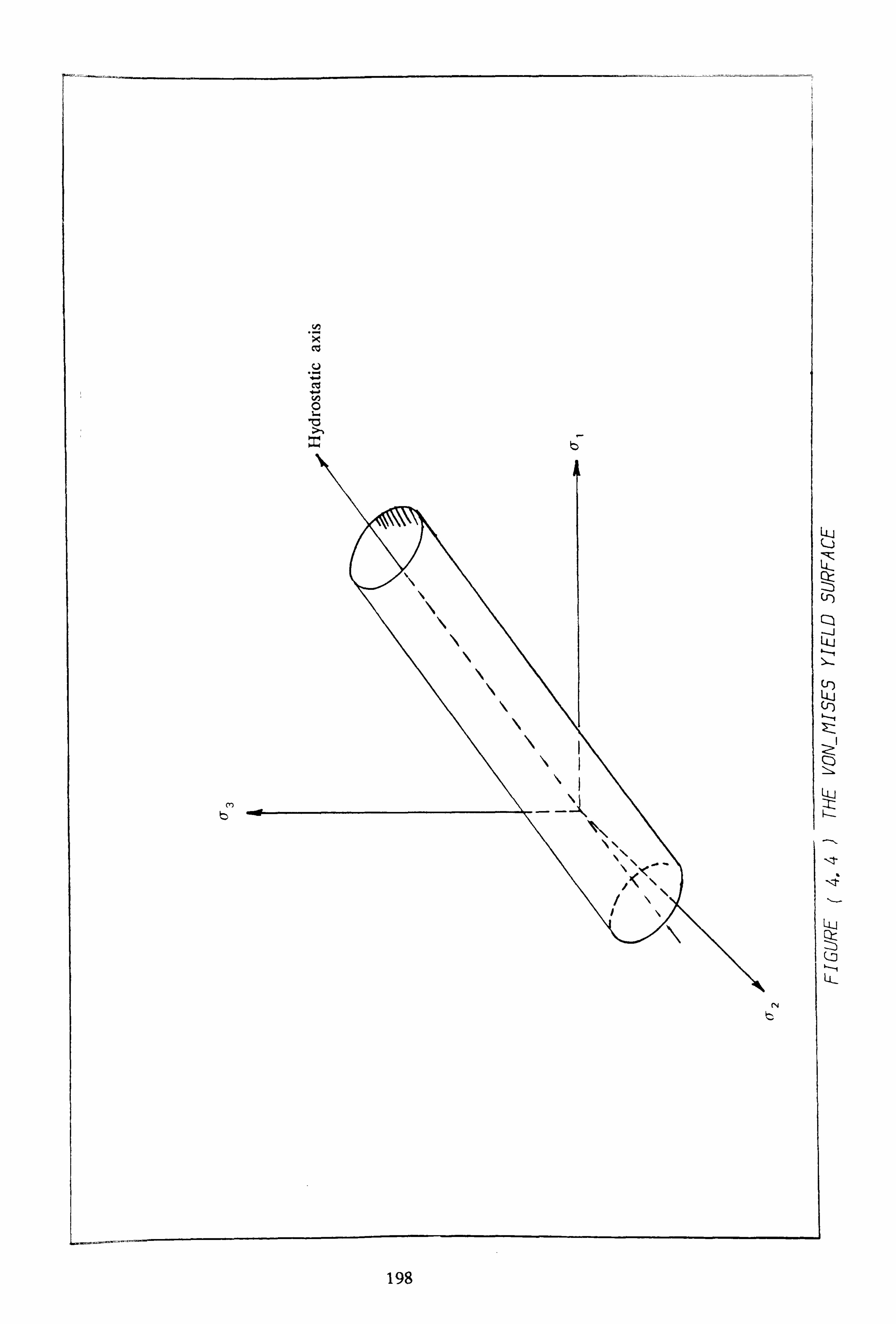
03

Cl)

ONO

LLJ

LL-

C)f :: j Cr) Cýl --i Lu

Lu

LI-i

LL-

198

Q. ) A / /

0 /

fl /

C

>

>

Q: Q LLJ

ýZý ýL-Lj

QL

: Z--

Cýl l---,

Ln

LQ

199

E

ol "a

7EL

cz

u

u

Dt

LLJ Qr

LL-

200

00,

. ooý . ",

I

-- ,I,

III, 1,1,1 ,III,

11 %\

Nl

(L)

CL 0

LLJ Q) It< QL

Zýl 6-4

LL,

: 2:

Lki "a k--: cx

Z

L. u -r

LIJ

clý :: 5

201

LU

tr

202

1-%

LLJ Q)

Qr-

Q)

L cx

Lu

Q: )

LU

Co

LLJ

PIS Ql)

uj il-1.

(71

203

I_ 0

C5 C)ý Z-11 Lu

C) C)t: Lij Z-

Lu

LLý , -- zr, LU

IL3

LL-

204

00,

LLJ

LLJ

LQ NZ

LU

Z-1

Zi

U-j

LL-

Lu

Q0 &--4 LL-

205

0.4 A ý

ý/ 17 / V)

Q-

r-L4

10-

ý)h- ct

ci

E3ý X) LLJ cx

LQ co L-Li

Lij

[Ij

Ot

Lt-

LLJ

206

L) ------.

---I

0 0

Zj Q) cn

Llu

Lu

ýE Pý

LLJ

Qj 1-1 LL-

207

C)

>I

Lu

---I CL Qý

Ql- Q- : ýh-

LLJ

I. S

CDC

LL-

208

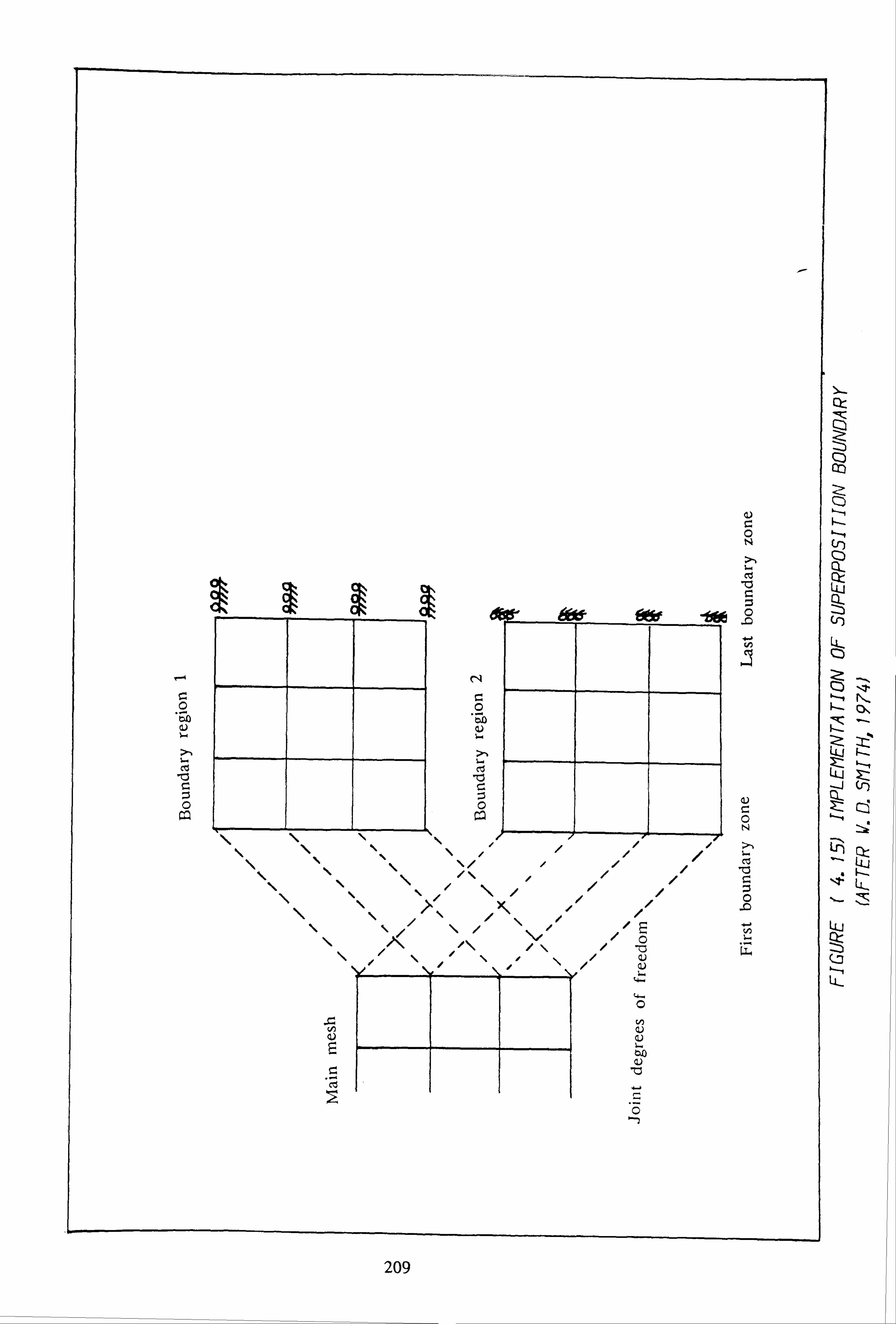
"a

ct

1>1 \/ oe

/ -0

I le Q)

Of

On

ZZ Q)

4j 0- zi (f)

LO

LU

LL

209

71

LN

cz u

ct

r- a

CO m 'tt 4 j, " ll: ý

210

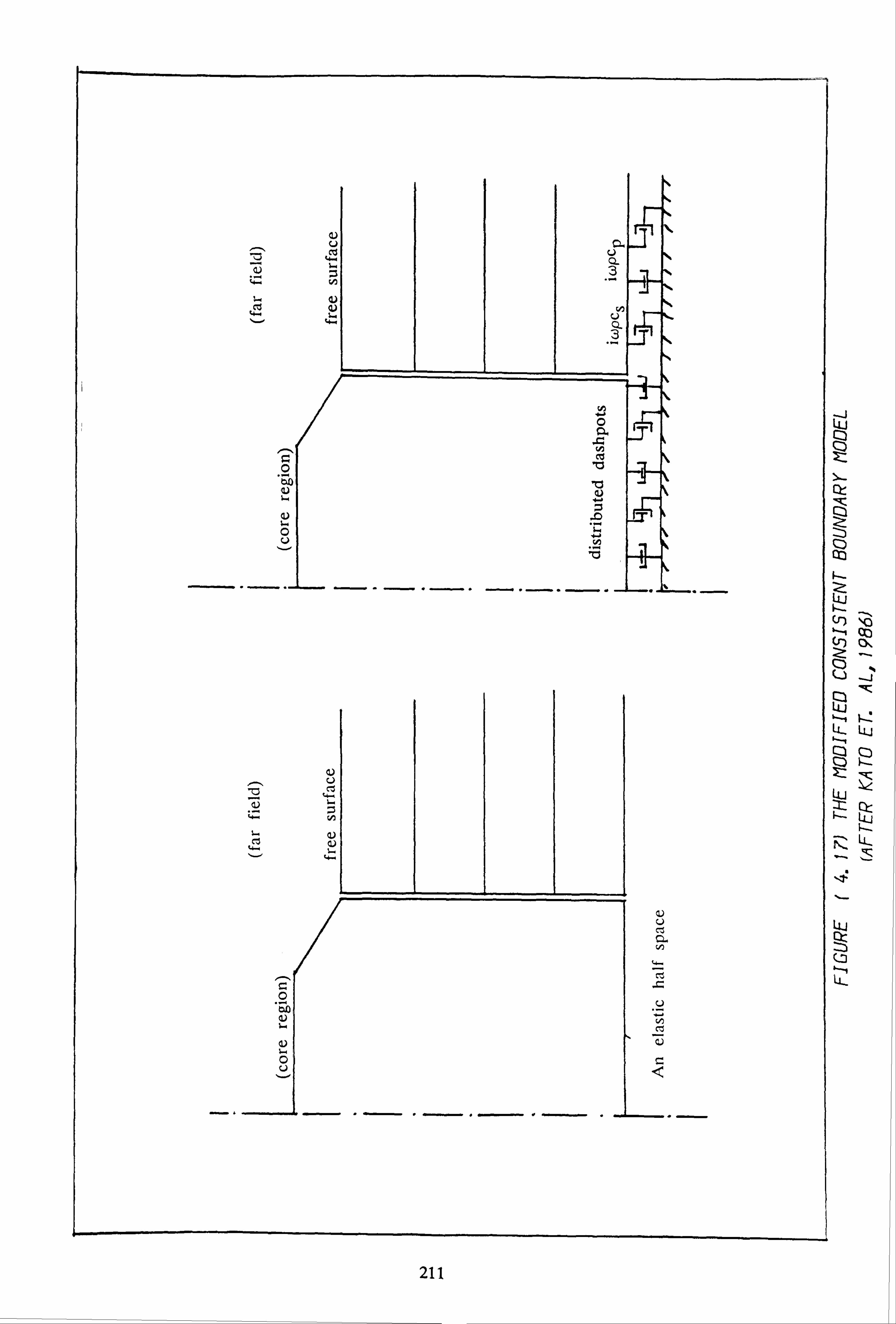
1211

H -N, 0 0

i ý to "o

(U

C"Z

ct

-i LLJ Q)

! LU

Qr) So -, Cc)

Qýl

Lul

LLJ

Z :ý T

clý U- Iýr IS

LL-

211

eel'@

2e, 4ýb

lp,

oll

I LL

LIJ Lu

LLJ

clý

212

U)

r ZX (D

ti

LO >1

<z co +r

:3 >-, N+

:3

co

+ 4ý-- - +X N

-. 1

Z

Ct

Q)

U-j 2

CL

LL

k-

LCJ d Lu Q. ) "'K

U-1-

LU

LL-

213

u

...............

(X)

: 2->

LQ Q-)

L, Lj

--l

LU

?s

214

ýe

Cýr

ON

c1c Q3

U-

Z: Lü ýd LLJ U l<

Z!, 1-4

S

LL-

215

4K

I%

XI 1'<

XI

'C 'C

F

Q) C. )

U

C. )

w

00

110

Itt

C14

H- r-

tn

CY)

M

"a

. ä.

0. )

ý1. >

216

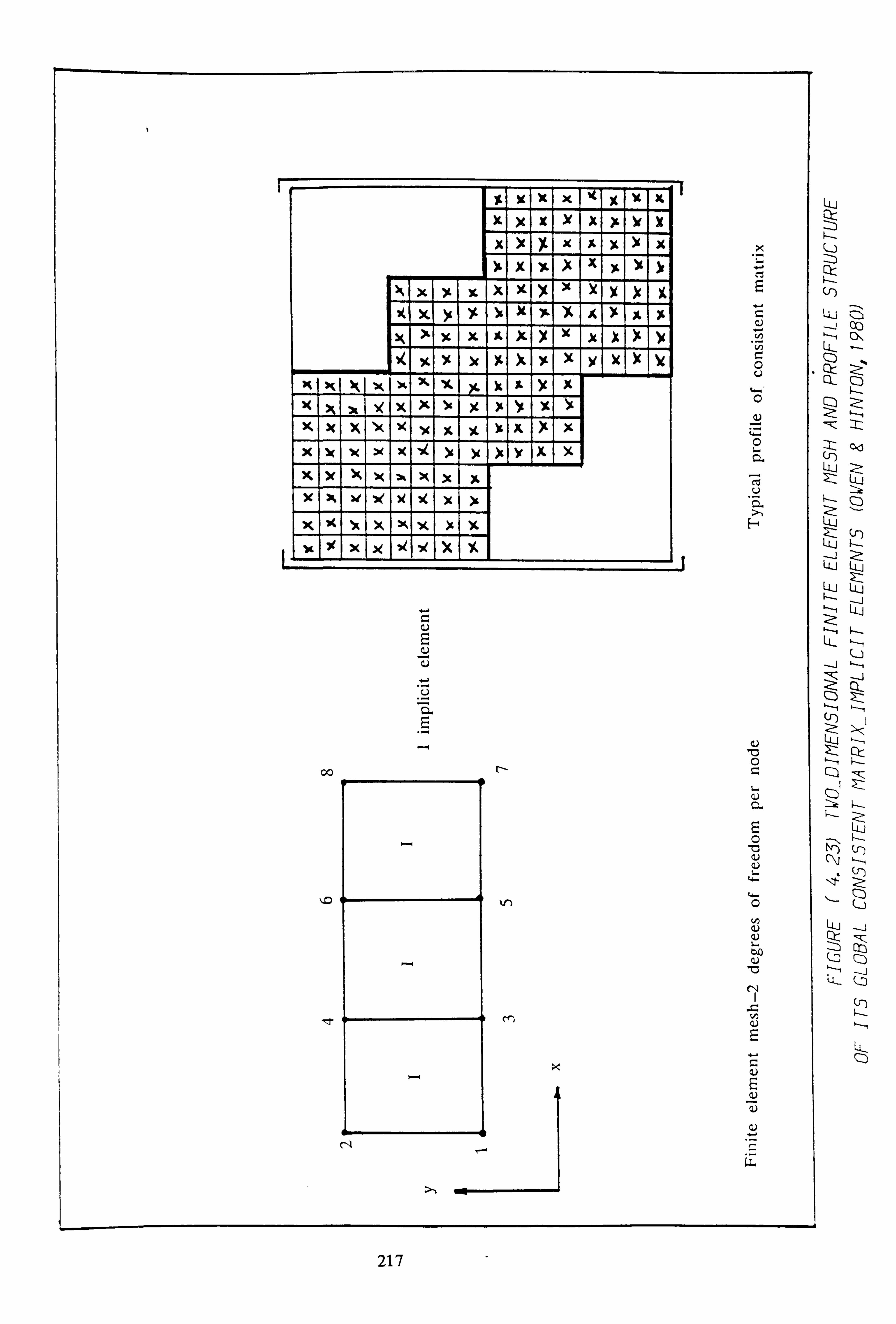
X x x 'A

xx x )( x A k

x x it x X x

)LI xI IL X Y. x

X )t y. XI Y-1 34 1

Y. )c I Y. )t X1 )L AI X X

X x it X1 )f x xI x -x

y x AxI 'A x I (I ), I lk

3K I *, 1 -4 1x Y-I 'K Y. IK JL y

x x

-)( XI )KI )c x )LI ),

)t Ix -A

X

A

,x x x x )(I -J, I )c I )gl v IX I

1ý1

x Iw )i

"a

"a

)t x x x 4 x x x x )( x A x x it x XI X1 )LI xI IL X Y. x

x )t I Y. XI Y-1 )( X1 341 x x

Y. )c I Y. )t I X1 )L x A I x x L M

x x

- -4 )c I 's x I x ju

.K XI *%I -A I XI ""I 'K Y. IK I JL )( x I

X1 )c x )' I)[ -A 'A

x -x I % x -j4l )c X x x X W W. 4( )i l< X )g

Lu )e jx jx

LQ

Co

00 cx

c: r- cl-

Z

Cr)

L-Li LLJ

LL-

Lu

: t3 cz

217

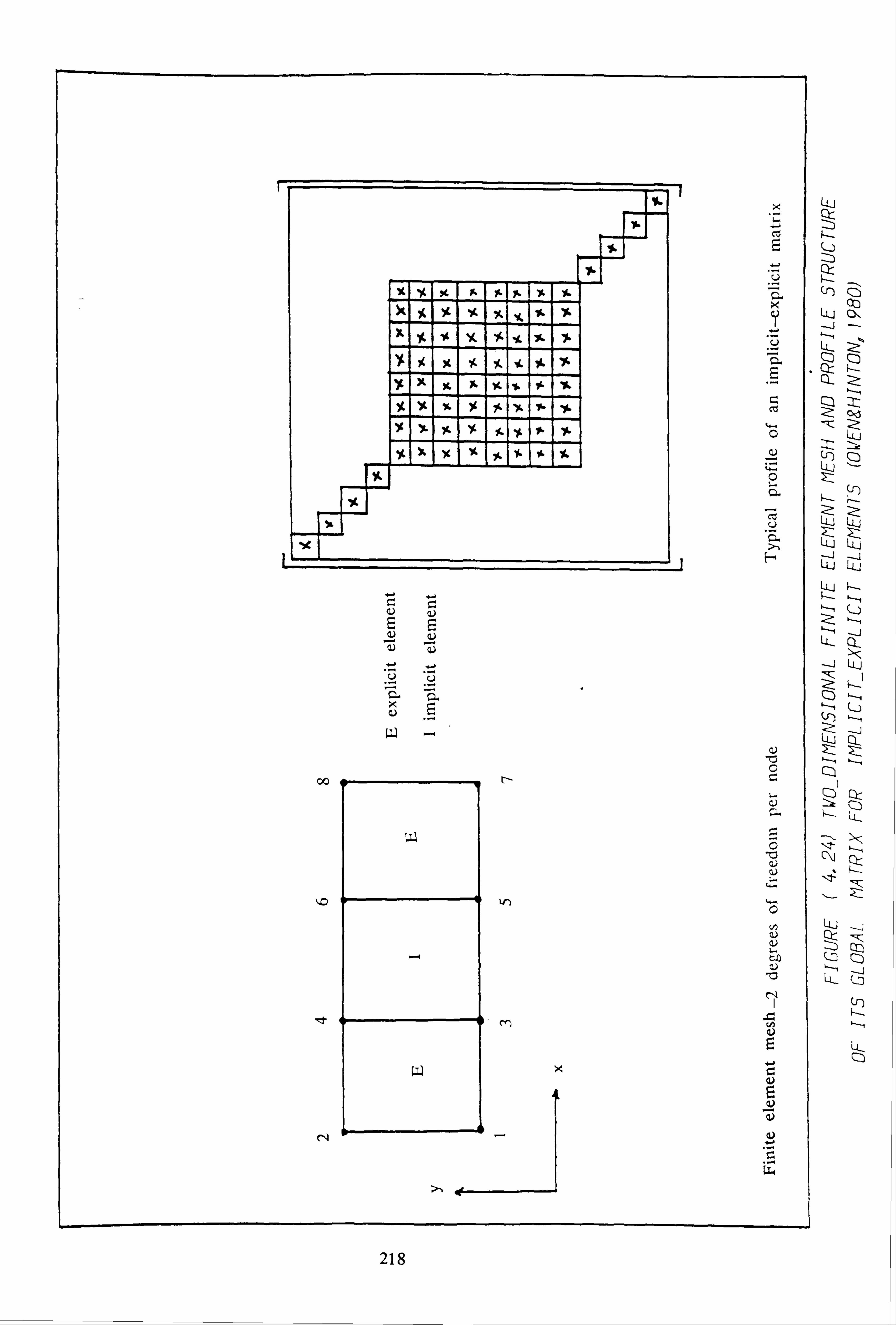
ct

)(f. %I -A Y I * -A I . V. y

7&

E

'06

0

IA

E

Z

00 10 r-

"0

U-i

PE co (Z)

CID LU cx

Cl- Z-

LQ

LU LU

LLI

C: ) -zit

C\j C)ý:

31ý Lj-j -: Q- Irr, :: 5 CQ

Q)

co

Lj-

C)

218

CHAPTER 5

FINITE ELEMENT ANALYSIS OF PILE DRIVTNG

5.1 INTRODUCTION

5.2 CONVERGENCE STUDIES

5.3 PARAMETRIC STUDIES

5.4 DISCUSSION

5.5 CONCLUSION

CHAPTER 5

FINITE ELEMENT ANALYSIS OF PILE DRIVTNG

5.1 INTRODUCTION

Until the finite element work of Chow (1981) and Smith and Chow (1982),

the pile driving problem had been analysed almost exclusively by means of one

dimensional models. In these simple models, stiffness and damping were simulated by means of springs and dashpots, attached at discrete points to the pile shaft and

pile base. As discussed earlier, this approach necessitates the use of essentially fictitious parameters. By contrast, the three-dimensional (axisymmetric) finite

element models make use of real soil properties (Young's modulus, mass density,

etc. ) and can therefore furnish a more realistic picture of the driving process.

No assumptions have to be made regarding the distribution of soil resistance along

the pile and both radiation and viscous damping can be accounted for in a

rational manner. The major disadvantage of the method, however, is that

computational times are prodigious.

One of the numerical difficulties arising in the application of the finite

element method to pile driving analysis occurs as a consequence of the very great

difference in stiffnesses between piles and typical soils. High frequency stress

waves may build-up in the pile since these can not propagate into the soil

elements (wavelengths in soil are much shorter). However, one method of

overcoming this difficulty is by introducing a small amount of damping at the

pile---soil interface to reduce the high frequency noise to an acceptable level while

only marginally affecting the overall pile response, Randolph and Simons (1986).

The only essential additional piece of information necessary to carry out a

dynamic finite element analysis (as opposed to a static analysis) is the soil mass

density. Special provision must be made however for damping at the boundaries

to prevent wave reflection and in order to reduce computational costs. It is only

feasible to analyse piles with circu lar cross sections, reducing the problem to an

axisymmetric one.

219

In this study, the soil has been modelled as non-viscous elastic, perfectly

plastic Von Mises material and the transmitting boundary in the far field has

been modelled using the viscous boundary devised by Lysmer and Kuhlemeyer

(1969) and modified by White et al, (1977). Allowance has been made for slip at

the pile soil interface at a specified value of skin friction, using Griffiths (1985)

thin eight noded, interface elements. A limited parametric study has been

conducted in order to gain some insight into the behaviour of the pile during the

driving process and to follow the evolution of failure in the soil around and beneath the pile.

During impact pile driving many modes of vibration will be excited. However, the higher modes in the discretised finite element system are likely to

be in error and there is little justification in including their contribution to the

response. Consequently, since a time integration scheme which possesses some

numerical damping has certain advantages, an unconditionally stable implicit

algorithm, namely the predictor-corrector scheme (developed by Hughes and Liu

(1978) and implemented by Owen and Hinton (1980) program MIXDYN), is used

to integrate the equations of motion in this study.

Initiation of the driving process can be performed by prescribing an initial

ram velocity or by specifying an appropriate forcing function based on hammer

manufacturer's force-time plots. In this Chapter, the latter method is preferred

(see also Borja, 1988; Shibata et al, 1989).

5.2 CONVERGENCE STUDIES

To verify the simulation of axial wave propagation down the pile (in the

absence of soil resistance) a simple test was carried out, as follows. Basically, a

uniform rod fixed at one end and free at the other was subjected to a suddenly

applied (and thereafter maintained) impact force (i. e. a Heaviside forcing

function). Wave propagation along the rod was examined with the use of , successively, 5,10 and 20 axisymmetric elements and by varying the length of the

time step. The effect of time step size and the number of elements is shown in

Figs. 5.1 to 5.9. Clearly, smaller time steps and more elements provide better

220

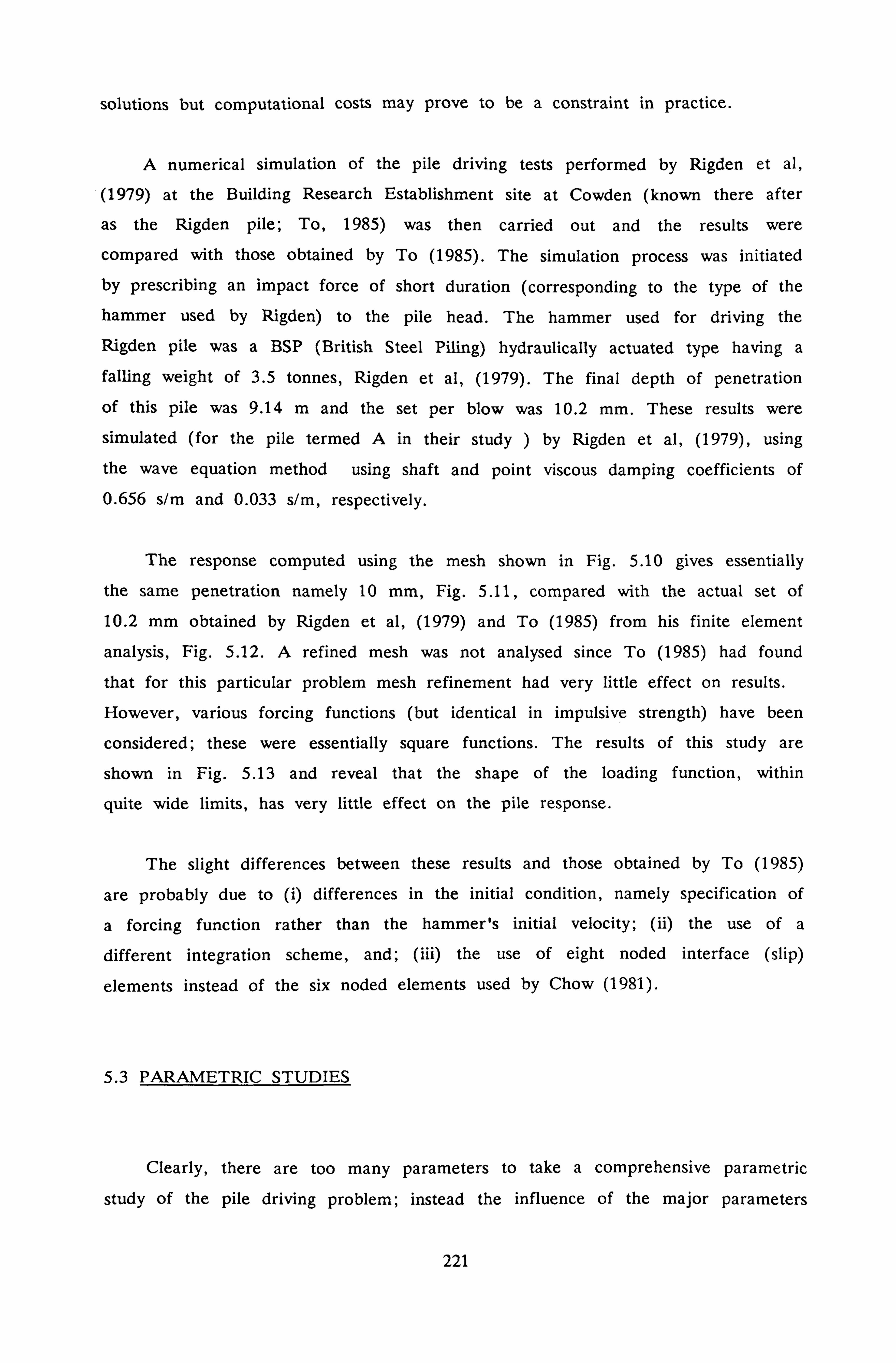
solutions but computational costs may prove to be a constraint in practice -

A numerical simulation of the pile driving tests performed by Rigden et al,

(1979) at the Building Research Establishment site at Cowden (known there after

as the Rigden pile; To, 1985) was then carried out and the results were

compared with those obtained by To (1985). The simulation process was initiated

by prescribing an impact force of short duration (corresponding to the type of the

hammer used by Rigden) to the pile head. The hammer used for driving the

Rigden pile was a BSP (British Steel Piling) hydraulically actuated type having a falling weight of 3.5 tonnes, Rigden et al, (1979). The final depth of penetration

of this pile was 9.14 m and the set per blow was 10.2 mm. These results were

simulated (for the pile termed A in their study ) by Rigden et al, (1979), using

the wave equation method using shaft and point viscous damping coefficients of 0.656 s/m and 0.033 s/m, respectively.

The response computed using the mesh shown in Fig. 5.10 gives essentially

the same penetration namely 10 mm., Fig. 5.11, compared with the actual set of

10.2 mm obtained by Rigden et al, (1979) and To (1985) from his finite element

analysis, Fig. 5.12. A refined mesh was not analysed since To (1985) had found

that for this particular problem mesh refinement had very little effect on results.

However, various forcing functions (but identical in impulsive strength) have been

considered; these were essentially square functions. The results of this study are

shown in Fig. 5.13 and reveal that the shape of the loading function, within

quite wide limits, has very little effect on the pile response.

The slight differences between these results and those obtained by To (1985)

are probably due to (i) differences in the initial condition, namely specification of

a forcing function rather than the hammer's initial velocity; (ii) the use of a

different integration scheme, and; (iii) the use of eight noded interface (slip)

elements instead of the six noded elements used by Chow (1981).

5.3 PARAMETRIC STUDIES

Clearly, there are too many parameters to take a comprehensive parametric

study of the pile driving problem; instead the influence of the major parameters

221

has been explored in typical cases. In this study, maximum pile segment lengths

of 1.0 m and a maximum transverse element dimension of 2.0 m; as shown in

Fig. 5.14, have been employed based on past experience. Further, in general,

time steps of 0.2 ms have been employed throughout.

The response of a concrete pile with an aspect ratio (L/d) of 20, and length

10 m, to impact is the main object of this study. The surrounding soil is

assumed to be a uniform saturated clay (variously assumed to have a stiffness (Young's modulus) of 2,10 and 50 MPa). The soil's undrained strengths are

computed from these stiffnesses by selecting a strength ratio 0 (= EsIcu);

typical values are 200,500 and 1000. The strength of the interface material is

defined by means of the adhesion factor a(= ca/cu); typical values are 0.1,

0.5 and 1.0. The applied impact pressure P is prescribed variously as 12 MPa, 23

MPa and 46 MPa, all acting for 5 ms ( i. e. as Heaviside functions) -

The primary parameters are thus four (4) in number, viz, the soil stiffness Es, the strength ratio 0, the adhesion factor ce and the hammer pressure P. The

mean values of each of these (namely, 10 MPa, 500,0.5, and 23 MPa) constitute

the "basic case" and while any three of these are held constant, the fourth may be varied to explore the sensitivity of the pile response to this parameter alone. The plots given here depict the variat ion of the mean and shear stresses beneath

the pile tip as a function of time and the evolution of failure within the soil.

Fig. 5.15 illustrates the influence of changing the adhesion factor a on the

maximum shear stress-time relationship. It is clear that the pile shaft adhesion

has no important effect on the shear stresses in the soil during driving. Failure in

the soil takes place after about 6 ms.

Fig. 5.16 depicts the mean stress-time relationship and reveals the greater

influence of the pile adhesion in this case. It also illustrates that this parameter

has no important effect on the soil mean stresses. The oscillations in these values

indicate that the pile itself vibrates during driving.

Fig. 5.17 shows the maximum shear stress-time relationship in the soil

underneath the pile tip as a function of the strength ratio, 0. This figure shows

that, as expected, soil strength has an important effect on the final state of the

soil after driving.

222

Fig. 5.18 shows the mean stress-time relationship in the same soils. Again,

soil strength has an important effect on the residual stress level in the soil after

driving.

The severe oscillations in these stress-time plots may be masked unless the

output is sampled at sufficiently fine intervals as depicted in Figs. 5.19 - 5.23

where the output is based on values calculated at, variously, 10,5,2 and 1 time

steps. The principal peaks in these response curves correspond to the return times for the applied stress wave reflected from the pile base.

Fig. 5.24 shows the maximum shear stress-time relationship in the soil

underneath the pile tip as a function of soil stiffness. The results show that the

change in soil stiffness has negligible effect on the response. This result is

confirmed by Fig. 5.25 which shows the mean stress-time relationship in the

same soil (element) underneath the pile tip.

The effect of increasing the pile head driving pressure on the maximum

shear stress and mean stress time relationships, respectively, is shown in Figs.

5.26 and 5.27. It is clear that the higher the driving pressure the higher will be

the residual shear stress after driving in the soil but the final mean stress is

largely unaffected by an increase in driving stress.

During pile driving, body waves and Rayleigh waves propagate radially out

ward from the pile along hemispherical wave fronts . This is shown in Fig. 5.28

for a circular surface footing on a homogeneous, isotropic elastic half-space

(Woods, 1968) subjected to forced excitation. Kezdi (1957,1975) has discussed the

effect of wave propagation during driving on a cohesionless soil and Taylor (1948)

has discussed the sequences of compression and disturbance occurring in clays during pile driving. Taylor's study concentrated on an analysis of changes in shear

strength. His conclusion that driving a pile in a soft impervious saturated clay

causes horizontal displacements has been confirmed by numerical results obtained by Chow (1981) and To (1985), in which they concluded that the displacement

vectors and yielding are localized underneath the pile.

The evolution of the yielding around and underneath the pile during and directly after driving is shown in Figs. 5.29 to 5.34. The yielding is indicated as

a 'dot' in the centroid of each element. It is clear that the yielding zone initiates

223

at the pile-. 6oil interface and then it propagates away from the pile, as time

proceeds. These bands appear to move a considerable distance out from the pile

and continue to do so for some time after impact has ceased.

5.4 DISCUSSION

As discussed in earlier Chapters, in a wave equation analysis, the permanent

set of the pile is determined by subtracting the quake value from the maximum displacement at the first peak (Smith, 1960). However, in the finite element

model, the permanent set of the pile is determined from the equilibrium position

of the pile tip, i. e. the computation proceeds until there is negligible movement

of the pile tip corresponding to a nearly zero velocity.

The impact loading is a large amplitude loading type and this may cause

changes in the soil structure strength. Many investigators (Richart et al, 1970)

have examined the dynamic stress-strain behaviour of soils using triaxial tests and

other means and these results should properly be incorporated into dynamic

analyses of pile driving. Casagrande and Shannon (1948) and Seed and Lundgern

(1954), found that this type of loading on saturated sand caused a typical increase

of strength ranging from 10-20%. Moreover, substantial increases of shear

strength of saturated clay were obtained by increasing the loading strain rate.

5.5 CONCLUSION

The Rigden pile (Rigden et al, 1979) previously analysed by To (1985) has

been re-analysed using a different interface element and a different time

integration scheme. The results obtained here were in very good agreement with

those obtained previously.

A parametric study of the behaviour of a driven concrete pile has been

carried out using a modified form of the Owen and Hinton (1981) MIXDYN

224

program. The principal modification, introduced into the program was the

inclusion of the Lysmer and Kuhlemeyer (1969) viscous boundary to prevent

spurious reflections at artificially curtailed boundaries.

The results indicated that neither pile shaft adhesion nor soil stiffness had

much effect on the stresses in the surrounding soil after driving but increases in

soil strength and ram force were found to have significant effects on the residual

stresses following impact. A study of the evolution of yielding around and

underneath the pile shows that the failure zone propagates a considerable distance

away from the pile shaft and continues to do so for some time after the ram

forces has subsided.

225

Cl

co

z Lr) LLI Q)

m+ U-j LU LLJ (Z) o:: LL-

LLJ

C: ) m LL-

Lij LLJ r,: ) U --j Z

., o U-)

-LIJ 11

Zo 7--

Ln

LU

--r I: r- -Q)

CL

Lri LL,

LQ

ý-z LLJ l-" Ll- I-

Cl

SSýýLALS ýVIXV 19VHýAV

226

Ln Ln C) I C; 6

Ei; -U) -En fb La. u tu

�pul , rL Ul U) (n tLi M c2 cl Czi CD ,e

-i L5 CD w LLJ Ln (n Ul) in

tn 0- ry CD 1

1-- ci d c: i

i .., # ,

%I %

Ln CD Ln Cl 16C;

SS3diS ýVIXV ýOYdýAY

0

CID

r-

C: ) Z: LU

LU LU CK LL-

LU

CD W- LL-

U. 3 u

cr)

Ln

IT

K)

CN

C3

>Z

Z

CL

Lu Qýl

It Lli

CL i

i. - 4 ; ZLij

5cO

Lri LLJ

(-j Lu

227

C

X Cl

uj Ln co LLJ +

ui cy-

LLJ U- ui

C: ) cl: U- U-i LLJ U

-j (Z. ý Z: ). ý

*10 F--4 LLJ ca 11

CL

Ln

Q, +

LLJ

Cý

cr) "ý, LO Lu : Eý Fý

C-73 Lo (f)

Lri + LJLJ

L? Lii

LL-

CD

663diS ýVIXY ý9Vd9AV

228

CD U-1 C) Ln Ln Cl Ki C%i rý -1

66

a

LL

co L&J LLJ

U. j

LL-

LLJ u

U) 10 F--4 lkJ 11

(zi

Ln

ILJ Qr

on 4

L4 IQ

Lul

a

MRIS -iYIXY -: IDV83AY

229

LF1

tn in in 0 vi in

Ls tj in

UU11 ýw

== H

u ig - cm U, CD

I- C; d C3 C;

13 -4

N

( I.,.

lolo

*I .A

*

Ln

ýýS38iS -IYIXY 35Vý30

uI C;

0

Ln OD

LU

LLI

U-

LLJ

rIL

LL

LLJ u = 1ýý , <

Lr)

Ln 44

LQ

U-1 Lri Lij

t-ý) LLJ ý--4 Ll- I--

0 lz;. A

C;

230

0

cm z LU

m (ZI LLJ + LU LLJ- cr- U-

LU

1: C: ) CL w U- LU Lij Uj

No LL,

E :ý LM

cis

LU

ce

Lu

LL4

LQ

0

SS3biS 'IVIXV 35Vb3AV

231

LM Ln 0

W5 NNdC;

0

I Ae :: ; "-

JK

Vic

-7--- -- --Ir ---- I Ln Cl Ln

SS26iS -lVIXV 2DY83AY

232

0% r-

C2 z LLI C,

+ LLJ LLJ LLJ Q,

LL-

LLI

0 LL. LLJ Uj cz, U Z

L

zz zi

Ln

+ LQ

IT Q- C5

LLJ

LU Z5 co LLJ LL-

CD

V) w CL CL

cn

u Li Uj u V) tn 1: (21 Ln C%j

LU cl

E5 x I-

I*f i:

'!:

ý 44 *4

IV)

06

Iýx

4%

I; x

. 10

% *4%

%%

t

WA i

------------

Wý: -*- . -. ýki

Ln Ln

SS28iS -IVIXV ýDVd9AV

233

Cl

Ol

-a

M

LLI OD

uj ILJ cr U-

LL1

CD CY- LL-

LU Z < uý

10 0W

Ln

-T Clý Ct CL cn Lr)

co

Lri

LQ

LL-

cl

Ln

II

Z: :: 3 Qý \1 Q3,

Qr)

11

CD

laz

Qs 2ý co C3 Ln LU Q,

m+ ui LU LLJ Q)

U-

F- CL

C: )

LL-i r,: ) U

LO

QJ- :j Z_-

Q)

Ln

+ LLJ CA- C5 QL

(x I- --

Lri Lý r-11 I%-

LLJ

Cl

S91diS ýVIXV 29MýAV

234

Cl Ln C) Ln C) Ln Cl w; cNj cli -1 d C;

LD

ý

cm I I i

, Z!

le, 1 v7

7 P11 F

:- 207E6 KN, M2

8-127M

FE a

,, R"FOR STATiC ANALYSI!

FOR DRIVING ANALYSI

FIGURE (5- 10) FINITE ELEMENT MESH FOR RIGOEN"S (1979)CLOSED ENDED PILE.

5E4KNIM 2

Ul N

C;

Q C%j

C;

Ln

cs

Ln a d

0 C)

C;

( *'VN' ) IN2W2: )Y-IdSIO

236

CNJ Cl OD Ic 0

C; ci ci C; ci

co C)

C)

00 (n 01ý cu -4

1 10 - a

0

-a Q)

(-%j

C3

4-1 C: )

C)

cz

4-j u co

co

cs

10

CD CD

CD

CD

CD

(Ni CD Co ýa -Ir (1-i C: ) CD

CD CD CD CD CD CD CD CD C: ) CD

(D cý c; (D c; c3

VW) IN3W33VýdS10

237

LU tf)

U-1

I--

LIJ U-) 71 CD 0- (r) LLJ

LLJ 7- U-j

QL

LL CD

71 CD Ln cy-

CD

Lri

I, -

LD

uuUU LJ Uj uj ui tn cn u, ) tn = 1: == Ln ci Ln oi

ft ft

CL cL a. i C%ja. ===

aA rý: vi uj Iu4a U) LLJ U U3 uj

cr cr cr ix -i =D --73 =3 =3 < ul En Cf) U7 :D Or) tr) tr) U) ý- Uj LLJ Uj Uj u (Z ck: cr- cx le CL CL CL CL

C: )

ci LLJ

r-L

Lij LLJ

(fý C: ý Lrl

d L-Li

C-) clý

Cl I\-

Lri QD Cl-I

Ln

Cý CD

z-

t , Cl CD

Cl CD

CD Cl

( "VII )

238

CD "0 IT N CD CD 10 cl c2

13 GEG c2 CD c; ddd ci cs c;

0%

E PILE = 25E3 MPA

PILE

OUTER OIA. = 0-5M

PENETRATION =10-OM

OVERALL PILE LENGTH = 10-OM

TIME STEP SQE

MA VELDCITIES INITIAI 43 usI up/S-. )

(SIS

LYSIS

I 8 -173 M

_PA 710 M PA ýM FA ý01 C 50M

0E 200 IES OOIE SON/1000 u SOIL/

ý5

CA 11 ý-5 /

0"l

FFESSURE =12MPA Z3MPA I 46MPA FOR

5 MSEC INITIAýýýITIES 2-5Mb-2

FOR STATIC ANALYSIS

FOR DRIVING ANALYSIS

Fl G. (5-OFINITE ELEMENT MESH FOR THE CONCRETE PILE

Ln C;

1 11

CL

LLJ Ln

Qa

"Cl L

Ln Q Lri

ri

LL-

Cl cl 8 Ln 0

( W*13S/N ) SS381S 8Y2HS WnWIXYW

240

(D

Cý 01

C;

(W MS/N ) GG2&S NV3W

ýQ

241

(X) Ln ý& K) rli CD ly

'3 -

_2

? '; -

>. 1-

y.

Ln Ln Ln Ln -4*

5! ýR ?n Ln a

( W*DS/N ) SS3HIS 8V3HS wnwixyw

CL

C; 1 110

Lu it

Li U. I

Zn 7K Lrl LLJ

Ln = C;

CS

-2 CD C;

Xt

LM

Id

(3

0

242

ýQ

lqz ý8

c

LLI cn - ull Lu

U-J CL ti

ýi ý; . wo-

., Li iý . X:

LO IRE

co

IL

(W TS/N ) SS381S NY3W

243

1

In

(D x

r24

UJ

93 e ze 8

LU

e

d1t

8

(W MG/N ) SSMIS dY3HG WnW I XYW

244

Ul Cl

x

(W IISIN ) 993HIS NV3W

Ln N

245

CD 't CD

K d

Q- 6-4

cL

L3 LLJ

uj

I. J4

Bi

zz

CX

Lri

0 Qj tz

(W "13S/N ) smis 8Y-3Hs wnwixvw 246

4;; -- - X. a; 1-

MP

-0

3: -. r: z -.

cl 4=1 cz in %0

----------- ------------ cm CD Cý cm CD Cý Cl 0 cn Cl Q CD C) cm ca C3 Cl 40 C21 Cl C2 Cl I= Cl CD C= C3 Cl Cl 40 C2 10 Cl CD M CD Ln Ul Cl 0M C3 M *0 Ln Ln *r -4r tn X)

iq CY Ln

(W *M/N ) SS3&S HUHS WrIWIXYW

CL

LO

Cl

li ;z ze C3

Lu 0

Q.

LLJ Ln

U. j r's in 3= W- C;

(Xo MIC 4-3 LU

c zo-,

Ln C; Lr

d 81-4 4-

Cl C3

c;

247

m

CD C) Ln

na

---- -. 0

%no

06 x

WTS/N ) SS381S NY3W

lc; l Ily

248

CL

ý-- -, a L-

Cl.

ul (n

uj

LA

u

LJ-

Qj

tz

0 0

S 0

(W TS/N ) 663diS 8Y3HS wnwixvw 249

CD

0 x

io c3 (n

10 10 w LU LD c3

Lfi

ui w Ui

c3

...........

.:: ----------

-. -. --- --Z.

-----------

.... Z--. . ..........

----------- - c3

---------- -

---------- '-.:: z: -----------

------- ýg

........

--- ------- ------------ --------

----------- ---------

--

-------------- ----------- =-=

-------- -

-- --- -------- -

------------- - ----------------- ......... -ýr n-, ý--, Z ------------- =U =-' -- -

ii11

x (W *OS A) SSMIS NY3W

250

%0 10 10 LLJ w

CL Z-

-------------- -----------

.... ... .......

---------- ..........

-- ------------------- ----------*

lý-

, 1. --,

- ----------- ----------

. -,

-v-u- *- -- --

--------- - »- -==Z::

----- ---- - -- ......... ----- ..... ::: --

-- -----------

..........

---

.

--------

-- ---------------- . ..........

. - - ................ - -- -------

--------- -------

- ------------ ------

--- -----

------------

-----------------

§§8 Ln 2 Cl

( W*DS/N ) SSMIS 8Y3HS WfIWIXYW

io ci

Ln

d

8

Id

Ck Cl

c;

cx.

LL,

Lu "

I 251

ra

252

e ýr r-i 0 v- CD 10 -t r43 ly

W *CS/N ) SS3&S NY3W

Q) -0

Cl. E

00 0)

C) 3: L2 h. - I/ ,

(7) 0

C, E 0 >u cx

0

3: Ln 0

3.1 E oE 0

- (L) 0 C) C) Q) C:

-C V)

a

0

cC cu LLJ

L)

0

c cl 0

Q) -C CP a Q) Cl

o -5, Q )E 00

-0

253

L&J

444

LLJ.

qiý. - VJ

CN

L4

Lri

254

. . S

J _

ýi 1-, -cr,

:e-, -

LQ

Lri

LL-

255

00

.. 0S0 .5S

1S

--i

tu. ull % lö-ý ; 41 ýý 00 its

Z)

L4

Lri %I-

256

-i -I

ý3 1-1 'Z

Lri N-

257

Zjj

0aI

li

k 6-ý

LU

LQ

Lxi

U-

258

004

0

4Ji--

qz-

3.

LLJ

259

CHAPTER 6

CONCLUSIONS AND RECOMMENDATIONS FOR FUTURE STUDIES,

6.1 CONCLUSIONS


CHAPTER 6

CONCLUSIONS AND RECOMNMNDATIONS FOR FUTURE STUDIES,

6.1 CONCLUSIONS,

The major thrust of this Thesis has been to compare alternative approaches

to the dynamic analyses of pile driving. The methods considered include the pile

driving formulae, single degree of freedom models, the wave equation method due

to Smith (1960) and the finite element method of analysis. The single degree of

freedom analysis (SDOF) involves the idealisation of the pile as a rigid mass

while the soil is modelled as a slider--spring-dashpot mechanism. The SDOF

model is probably comparable in accuracy to the well-known pile driving

formulae, but it is not adequate from the practical point of view except perhaps

for piling in very soft soils.

A computer program was developed based on the numerical solution of the

wave equation described by Smith (1960) and a parametric study of the major

hammer, cushion, pile and soil characteristics was undertaken. The results were

compared with those obtained from the SDOF models and showed that pile

compressibility was an important factor in pile driving performance. Basically rigid

piles (SDOF) can be driven further into the ground than compressible piles.

From the results of the parametric study a new "pile driving formula", was

developed which appears to give useful results. However, it is doubtful whether

any simple analytical formula can provide results of wide generality.

Modelling of soil behaviour during pile driving should include the effect of

remoulding and pore water pressure generation but these cannot be readily

incorporated into numerical calculations. Thus the analyses in this Thesis are

based on a total stress approach using the elastic -perfectly plastic Von Mises

model as a description of the behaviour of saturated clay soils.

260

The dynamic finite element analyses of pile driving allows the soil to be

explicitly included in the analysis using meaningful soil parameters and provides a

more rigorous solution than either the elementary models or Smith's (1960) wave

equation method. An implicit temporal integration is used since the relatively large time step sizes results in substantial cost savings by comparison with explicit

schemes. However, computational costs are two or three orders of magnitude higher than those incurred in carrying out wave equation analyses.

The finite element analysis showed the evolution of the yielding zone around

and beneath the pile propagating outwards from the pile directly after impact in

the form of bands to some considerable distance.


The Von Mises model has been used to simplify matters in this Thesis but

the use of more sophisticated soil models (such as the Critical State Model) would

give further insights into the behaviour of soils around driven piles during the

driving process. This would allow some progress to be made into the problem of

predicting pile "set-up" due to the reconsolidation of soils subsequent to pile

driving.

There is also an urgent need to reduce computational costs and to that end

utilisation of parallel processor technology may be useful although in the short

term a more effective solution may be to develop boundary element solution

algorithms. Possibly a hybrid FEM/BEM approach in which the far-field is

represented by the boundary elements would be most effective strategy.

261

REFERENCES

AGERSCHOU, H. A. (1962) "Analysis of the Engineering News pile formula, "

Journal of the Soil Mechanics and Foundation Division, Proceedings of The

American Society of Civil Engineers, vol. 88, No. SM5, pp. 1-11.

AKIYOSHI, T. (1978) "Compatible viscous boundary models, " Journal of the

Engineering Mechanics Division, Proceedings of The American Society of Civil

Engineers, vol. 104, No. EM5, pp. 1253-1266.

ANGELIDES, D. C. and ROESSET, J. M. (1980) "Non-linear dynamic stiffness of

piles, " Research Report R80-13, Civil Engineering Department Massachusetts

Institute of Technology, USA.

ATKINSON, J. H. and BRANSBY, P. L. (1978) "The Mechanics of Soils" an Introduction to Critical State Soil Mechanics, " McGraw Hill Book Co., London.

AUTHIER, J. and FELLENIUS, B. H. (1980) "Quake values determined from

dynamic measurements, " International Seminar on The Application of Stress Wave

Theory on Piles/ Stockholm / 4-5 June, pp. 197-216.

BATHE, K-J. and WILSON, E. L. (1976) "Numerical Methods in Finite Element

Analysis, " Prentice-Hall Inc., Englewood Cliffs, New Jersey, USA.

BETTESS, P. and ZIENKIEWICZ, O. C. (1977) "Diffraction and refraction of

surface waves using finite and infinite elements, " International Journal for

Numerical Methods in Engineering, vol. 11, pp. 53-64.

BORJA, R. I. (1988) "Dynamics of pile driving by the finite element method, "

Computers and Geotechnics, vol. 5, pp. 39-49.

BRITTO, A. M. and GUNN, M. J. (1987) "Critical State Soil Mechanics via Finite

Elements, " Ellis Horwood Ltd., Chichester, West Sussex, England, U. K.

BURLAND, J. B. (1965) "The yielding and dilation of clay, correspondence, "

262

Geotechnique, vol. 15, pp. 211- 214.

CASAGRANDE, A. and SHANNON, W. L. (1948) "Stress deformation and

strength of soils under dynamic loads, " Proceedings of 2nd International

Conference on Soil Mechanics and Foundation Engineering, ICSMFE, vol. V, pp. 29-34.

CELEP, Z. and BAZANT, Z. P. (1983) "Spurious reflection of elastic waves due

to gradually changing finite element size, " International Journal for Numerical

Methods in Engineering, vol. 19, pp. 631-646.

CHELLIS, R. D. (1961) "Pile Foundations, " Ch. 7 in Foundation Engineering, ed. by G. A. Leonards, McGraw-Hill, New York, USA.

CHOW, Y. K. (1981) "Dynamic behaviour of piles, " Ph. D. Thesis, Manchester

University, England, U. K.

CHOW, Y. K. and SMITH, I. M. (1981) "Static and periodic solid infinite

elements, " International Journal for Numerical Methods in Engineering, vol. 17,

pp. 503- 526.

CHOW, Y. K. and SMITH, I. M. (1984) "A numerical model for analysis of pile driveability, " Proceedings of 2nd International Conference on The Application of Stress Wave Theory on Piles/ Stockholm / 27-30 May, pp. 319-325.

CORTE, J. -F. and LEPERT, P. (1986) "Lateral resistance during driving and dynamic pile testing, " Proceedings of 3rd International Conference on Numerical

Methods in Offshore Piling / Nantes-France / 21-22 May, pp. 19-33.

COSTANTINO, C. J. (1967) "Finite element approach to stress wave problems, "

Journal of the Engineering Mechanics Division, Proceedings of The American

Society of Civil Engineers, vol. 93, pp. 153-176.

COYLE, H. M. and REESE, L. C. (1966) "Load transfer for axially loaded piles in

clay, " Journal of the Soil Mechanics and Foundation Division, Proceedings of The

American Society of Civil Engineers, vol. 92, No. SM2, pp. 1-26.

263

COYLE, H. M. and GIBSON, G. G. (1970) "Empirical damping constants for sand

and clays, " Journal of the Soil Mechanics and Foundation Division, Proceedings

of the American Society of Civil Engineers, vol. 96, No. SM3, pp. 942-965.

COYLE, H. M., LOWERY, Jr., L. L. and HIRSCH, T. J. (1977) "Wave equation analysis of piling behaviour, " Ch. 8 in Numerical Methods in Geotechnical

Engineering, ed. by DESAI, C. S. and CHRISTIAN, J. T., McGraw Hill Book Co.,

New York, USA.

CUNDALL, P. A., KUNAR, R. R., CARPENTER, P. C. and MARTI, J. (1978) "

Solution of infinite dynamic problems by finite modelling in the time domain, " Conference on Applied Numerical Modelling, Madrid, Sept.

CUMMINGS, A. E. (1940) "Dynamic pile driving formulas, " Journal of Boston Society of Civil Engineers, vol. 27, pp. 6-27.

DAVIES, T. G. (1979) "Linear and non-linear analysis of pile groups, " Ph. D.

Thesis, University College Cardiff, Wales, U. K.

DAVIES, T. G. and BANERJEE, P. K. (1980) "Constitutive relationships for ocean

sediments subjected to stress and tempereature gradients, " Report No. AERE-R

9775 for U. K. Atomic Energy Authority, HARWELL, Oxfordshire.

DESAI, C. S. and CHRISTIAN, J. T. (1977) "Numerical Methods in Geotechnical

Engineering, " McGraw Hill Book Co., New York, USA.

DESAI, C. S. and GALLAGHER, R. H. (1983) editors of Proceedings, International

Conference on Constitutive Laws for Engineering Materials-Theory and

Application, 10-14 Jan. Arizona.

DESAI, C. S. and SAXENA, S. K. (1981) editors of Proceedings, Symposium on

Implementation of Computer Procedures and Stress-Strain Laws in Geotechnical

Engineering, Chicago, 3-46 August.

DESAI, C. S. and SIRIWARDANE, H. J. (1984) "Constitutive Laws for Engineering

Materials, with Emphasis on Geologic Materials, " Prentice-Hall, Inc., Englewood

Cliffs, New Jersey, USA.

264

DESAI, C. S., ZAMAN, M. M., LIGHTNER, J. G. and SIRIWARDANE, H. J.

(1984) "Thin layer element for interfaces and joints, " International Journal for

Numerical and Analytical Methods in Geomechanics, vol. 8, pp. 19-43.

ERINGEN, A. C. and SUHUBI, E. S. (1974) "Elasto Dynamics, " Vol. I& Vol. 11,

Academic Press, New York, USA.

EBECKEN, N. F. E., LIMA, E. C. P., LANDAU, L. and COUTINHO, A. L. G. A.

(1984) "Numerical simulation of pile driving by finite elements; some applications

on the Brazilian coast, " Proceedings 2nd International Conference on The

Application os Stress Wave Theory on Piles/ Stockholm/ 27- 30 May,

pp. 350- 359.

FLAATE, K. (1964) "An investigation of the validity of three pile driving

formulae in cohesionless materials, " Norwegian Geotechnical Institute, Publications

No. 56, pp. 11- 22.

FOREHAND, P. W. and REESE, Jr., J. L. (1964) "Prediction of pile capacity by

the wave equation, " Journal of the Soil Mechanics and Foundation Division,

Proceedings of The American Society of Civil Engineers, vol. 90, No. SM2, pp. 1-25.

FOX, E. N. (1932) "Stress phenomena occuring in pile driving, " Engineering, vol. 134,2nd Sept., pp. 263-265.

GHABOUSSI, J., WILSON, E. L. and ISENBERG, J. (1973) "Finite element for

rock joints and interfaces, " Journal of the Soil Mechanics and Foundation

Division, Proceedings of The American Society of Civil Engineers, vol. 99, No.

SM10, pp. 833-848.

GOBLE, G. G. and RAUSCHE, F. (1976) "WEAP - wave equation analysis of

pile driving, " Vol. I-III, Report No. FHWA IP-76-14, Federation Highway

Administration, July.

GOBLE, G. G., RAUSCHE, F. and LINKINS, Jr., G. E. (1980) "The analysis of

pile driving, a state-of-the-art, " International Seminar on The Application of Stress Wave Theory on Piles / Stockholm / 4-5 June, pp. 131-161.

265

GOODMAN, R. E., TAYLOR, R. L. and BREKKE, T. L. (1968) "A model for the

mechanics of jointed rock, " Journal of the Soil Mechanics and Foundation


SM3, pp. 637- 659.

GRAFF, K. F. (1975) "Wave Motion in Elastic Solids, " Ohio State University

Press, USA.

GRIFFITHS', D. V. (1985) "Numerical modelling of interfaces using conventional finite elements, " Proceedings of 5th International Conference on Numerical

Methods in Geomechanics / Nagoya-Japan / 1- 5 April, pp. 837- 844.

HANNIGAN, P. I. (1984) "Large quake development during driving of low

displacement piles, " Proceedings of 2nd International Conference on Application of Stress Wave Theory on Piles / Stockholm / 27-30 May, pp. 118-125.

HANSEN, L. A. and SCHROEDER, W. L. (1977) "Penetration resistance for driven

piling, " Journal of the Construction Division, Proceedings of The American

Society of Civil Engineers, vol. 103, No. C03, pp. 513-528.

HEUZE, F. E. and BARBOUR, T. G. (1982) "New models for rock joints and

interfaces, " Journal of the Geotechnical Engineering Division, Proceedings of The

American Society of Civil Engineers, vol. 108, No. GT5, pp. 757- 776.

HILBER, H. M., HUGHES, T. J. R. and TAYLOR, R. L. (1977) "Improved

numerical dissipation for time integration algorithms in structural dynamics, "

Earthequake Engineering and Structural Dynamics, vol. 5, No. 3, pp. 283-292.

HILEY, A. (1930) "Pile driving calculations with notes on driving forces and

ground resistance, 11 The Structural Engineer, vol. 8, July-August.

HILL, R. (1950) "The Mathematical Theory of Plasticity, " Pergamon Press, U. K.

HINTON, E. and OWEN, D. R. J. (1977) "Finite Element Programming, "

Academic Press, London.

HIRSCH, T. J., LOWERY, L. L., COYLE, H. M. and SAMSON, C. H. (1970) "Pile

266

driving analysis by one dimensional wave theory :A state of the art, " Highway

Research Record, No. 333, pp. 33- 54.

HOLMES, N. and BELYTSCHKO, T. (1976) "Postprocessing of finite element

transient response calculations by digital filters, " Computers and Structures, vol. 6,

pp. 211- 216.

HOUSEL, W. S. (1966) "Pile load capacity estimates and test results, " Journal of

the Soil Mechanics and Foundation Division, Proceedings of the American Society

of Civil Engineers, vol. 92, No. SM4, pp. 1-29.

HUGHES, T. J. R. and LIU, W. K. (1978a) "Implicit-Explicit finite elements in

transient analysis : stability theory, " Journal of Applied Mechanics,

Transactions of the American Society of Mechanical Engineers, vol. 45, pp. 371-374.

HUGHES, T. J. R. and LIU, W. K. (1978b) "Implicit-Explicit finite elements in

transient analysis : Implementation and numerical examples, " Journal of Applied

Mechanics, Transactions of The American Society of Mechanical Engineers, vol.

45, pp. 375- 378.

ISAACS, D. V. (1931) "Reinforced concrete pile formulas, " Transactions of The

Institute of Engineers, Australia, vol. 12, pp. 313-323.

ISENBERG, J. and VAUGHAN, D. K. (1981) "Non-linear effects in soil structure

interaction, " Proceedings Symposium on Implementation of Computer Procedures

and Stress-Strain Laws in Geotechnique Engineering / Chicago-Illinois / ed. by

DESAI and SAXENA, vol. 1, pp. 29-45.

KATO, S., SOHRI, T. and GOULD, P. L. (1986) "A modified thin-layered far

field soil element for soil structure interaction of axisymmetric structures, "

Computer and Geotechnics, vol. 2, pp 167-184.

KAUSEL, E. (1974) "Forced vibrations of circular foundations in layered media, "

MIT Research Report RT74-11, Soil Publication No. 336, Structures Publication

No. 384, Massachusetts Institute of Technology, Cambridge, Mass., USA.

267

KATONA, M. G. (1983) "A simple contact friction interface element with

application to buried culvert, " International Journal for Numerical and Analytical

Methods in Geomechanics, vol. 7, pp. 371-384.

KEZDI, A. (1957) "Bearing capacity of piles and pile groups, " Proceedings 4th

International Conference Soil Mechanics and Foundations Engineering, vol. 2, ICE,

London, pp. 46- 51.

KEZDI, A. (1975) "Pile foundations, " Ch. 19 in Foundation Engineering Handbook, ed. by H. F. Winterkorn and H-Y Fang; Published by Van Nostrand Reinhold Co., N. W.

KUHLEMEYER, R. L. (1979) "Vertical vibration of piles, " Journal of Geotechnical

Engineering Division, Proceedings of The American Society of Civil Engineers,

vol. 105, No. GT2, pp. 273-287.

LEE, S. L., CHOW, Y. K., KARUNARATNE, G. P. and WONG, K. Y. (1988)

"Rational wave equation model for pile driving analysis, " Journal of the Geotechnical Engineering Division, Proceedings of The American Society of Civil

Engineers, vol. 114, No. GE3, pp. 306-325.

LITKOUHI, S. and POSKITT, T. J. (1980) "Damping constants for pile driveability calculations, " Geotechnique, vol. 30, No. 1, pp. 77-86.

LYSMER, J. and KUHLEMEYER, R. L. (1969) "Finite dynamic model for infinite

media, " Journal of the Engineering Mechanics Division, Proceedings of The

American Society of Civil Engineers, vol. 95, No. EM4, pp. 859-877.

LYSMER, J., UDAKA, T., TSAI, C. F. and SEED, H. B. (1975) "FLUSH

computer program for approximate 3-D analysis of soil structure interaction

problems, " Report No. EERC 65-30, University of California, Berkely, USA.

LYSMER, J. and WAAS, G. (1972) "Shear waves in plane infinite structure, "

Journal of the Engineering Mechanics Division, Proceedings of The American

Society of Civil Engineers, vol. 98, No. EM1, pp. 85-105.

MURAYAMO, S. and SCHOFIELD A. N. (1977) " Constitutive equations of soils, "

268

Special session 9, Proceedings, 9th ICSMFE, vol. 3, pp. 537- 546, Tokyo.

NAYLOR, D. J. and PANDE, G. N. (1981) "Finite Elements in Geotechnical

Engineering, " Pineridge Press, Swansea, Wales, U. K.

NEWMARK, N. M. (1959) "A method of computation for structural dynamics, " Journal of the Engineering Mechanics Division, Proceedings of the American Society of Civil Engineers, vol. 85, No. EM3, pp. 67-94.

NOGAMI, T. and KONAGAI, K. (1987) "Dynamic response of vertically loaded

non-linear pile foundation, " Journal of the Geotechnical Engineering Division,

Proceedings of the American Society of Civil Engineers, vol. 113, No. GT2, pp. 147-160.

NOVAK, M. (1977) "Vertical vibration of floating piles, " Journal of the Engineering Mechanics Division, Proceedings of The American Society of Civil

Engineers, No. EM 103, pp. 153-168.

NOVAK, M. (1985) "Analysis of hammer foundations, " Proceeding of 2nd

International Conference for Dynamics and Earthquake Engineering, June-July a board QE 2, NY to Southampton, CML Publications, pp. 4.60-4.70.

OLSEN, R. E. and FLAATE, K. S. (1967) "Pile driving formulas for friction piles

in sand, " Journal of the Soil Mechanics and Foundation Division, Proceedings of

The American Society of Civil Engineers, vol. 93, No. SM5, pp. 59- 73.

OWEN, D. R. J. and HINTON, E. (1980) "Finite Element in Plasticity, Theory

and Practice, " Pineridge Press, Swansea, Wales, U. K.

PALMER, A. C. (1973) editor of Proceedings, Symposium on Role of Plasticity in

Soil Mechanics, Cambridge, 13-15 Sept.

PANDE, G. N. and SHARMA, K. J. (1979) "On joint/interface elements and

associated problems of numerical ill--conditioning, " International Journal of

Numerical Methods in Geomechanics, vol. 14, pp. 293-300.

PARRY, R. G. H. (1972) editor of Proceedings, Roscoe Memorial Symposium:

269

Stress-Strain Behaviour of Soils, Henley-on-Thames, Foulis, USA.

POULOS, H. G. and DAVIS, E. H. (1980) "Load Capacity by Dynamic Methods, "

ChA in Pile Foundation Analysis and Design, John Wiley and Sons., New York,

USA.

RANDOLPH, M. F., CARTER, J. P. and WROTH, C. P. (1979) "Driven piles in

clay - the effect of installation and subsequent consolidation, " Geotechnique, vol. 29, No. 4, pp. 361- 393.

RANDOLPH, M. F. and SIMONS, H. A. (1986) "An improved soil model for one dimensional pile driving analysis, " Proceedings of 3rd International Conference on Numerical Methods in Offshore Piling/ Nantes-France / 21-22 May, pp. 3-17.

RAUSCHE, F., MOSES, F. and GOBLE, G. G. (1972) "Soil resistance predictions from pile dynamics, " Journal of the Soil Mechanics and Foundation Division,

Proceedings of The American Society of Civil Engineers, vol. 89, No. SM9, pp. 917-937.

RAUSCHE, F., GOBLE, G. G. and LINKINS, G. E. (1985) "Dynamic

determination of pile capacity, " Journal of Geotechnical Engineering Division,

Proceedings of The American Society of Civil Engineers, vol. 111, No. GT3,

pp. 367- 383.

RAO, S. S. (1982) "The Finite Element Method in Engineering, " Pergamon Press,

Oxford.

RICHART, Jr., F. E. (1962) "Foundation Vibrations, " Transactions of The

American Society of Civil Engineers, vol. 127, part 1, pp. 863-898.

RICHART, Jr., F. E. and WHITMAN, R. V. (1967) "Comparison of footing

vibration tests with theory, " Journal of the Soil Mechanics and Foundation


SM6, pp. 143-168.

RIGDEN, W. J., PETTIT, J. J., St. JOHN, H. D. and POSKITT, T. J. (1979)

"Developments in piling for Offshore structures, " BOSS'79, Proceedings of 2nd

270

International Conference on Behaviour of Offshore Structures, Imperial College,

London, 28-31 Aug., pp. 279-296.

ROSCOE, K. H., SCHOFIELD, A. N. and WROTH, C. P. (1958) "On the yielding

of soils, " Geotechnique, vol. 8, pp. 22-53.

SAMSON, C. H., HIRSCH, T. J. and LOVYTRY, L. L. (1963) "Computer study of

dynamic behaviour of piling, " Journal of the Structural Division, Proceedings of

The American Society of Civil Engineers, vol. 89, No. ST4, pp. 413-449.

SCHOFIELD, A. N. and WROTH, C. P. (1968) "Critical State Soil Mechanics, "

McGraw Hill Book Co., London.

SEED, H. B. and IDRISS, I. M. (1970) "Soil moduli and damping factors for

dynamic response analysis, " Report No. EERC 70-10, University of California,

Berkeley, USA.

SEED, H. B. and LUNDGREN, R. (1954) "Investigation of the effect of transient

loading on the strength and deformation characterstics of saturated sands, "

Proceedings of the American Society for Testing and Materials, ASTM, vol. 54,

pp. 1288- 1306.

SHANTARAM, D., OWEN, D. R. J. and ZIENKIEWICZ, O. C. (1976) "Dynamic

transient behaviour of two- and three-dimensional structures including plasticity,

large deformation effects and fluid interaction, International Journal of

Earthquake Engineering and Structural Dynamics, vol. 4, pp. 561- 578.

SHIBATA, T., SEKIGUCHI, H., MATSUMOTO, T., KITA, K. and

MOTOYAMA, S. (1989) "Pile driveability assessment by wave form analysis, "

Proceedings of 12th International Conference on Soil Mechanics and Foundation

Engineering, ICSMFE, Rio de Janeiro-Brazil, pp. 1-14/4-14.

SHIPLEY, S. A., LEISTNER, H. G. and JONES, R. E. (1968) "Elastic wave

propagation -a comparison between finite element predictions and exact

solutions, " Proceedings International Symposium on Wave Propagation and

Dynamic Properties of Earth Materials, 23-25 Aug., University of New Mexico

Press, pp. 509-519.

271

SIMONS, H. A. (1985) "A theoretical

University of Cambridge, England, U. K.

study of pile driving, " Ph. D. Thesis,

SIMONS, H. A., and RANDOLPH, M. F. (1986) "Comparison of transmitting

boundaries in dynamic finite element analyses using explicit time integration, "

International Journal for Numerical and Analytical Methods in Geomechanics, vol. 10, pp. 329- 342.

SMITH, E. A. L. (1955) " Impact and longitudinal wave transmission, " Transactions

of The American Society of Mechanical Engineers, Aug., pp. 963-973.

SMITH, E. A. L. (1960) "Pile driving analysis by the wave equation, " Journal of

the Soil Mechanics and Foundation Division, Proceedings of The American Society

of Civil Engineers, vol. 86, No. SM4, pp. 35-61.

SMITH, I. M. (1976) "Finite element analysis of axially loaded pile capacity and driveability, " Report to Fugro-Cesco B. V., March.

SMITH, I. M. (1978) "Transient phenomena of Offshore foundations, " Ch. 15 in

Numerical Methods in Offshore Engineering, ed. by O. C. ZIENKIEWICZ, R. W.

LEWIS and K. G. STAGG, Pub. by John Wiley and Sons., London.

SMITH, I. M. (1981) " Some time dependent soil-structure interaction problems, "

Ch. 8 in Finite Element in Geomechanics, ed. by G. GUDEHUS, pp. 251-291.

SMITH, I. M. (1982) "Programming The Finite Element Method with Application

to Geomechanics, " John Wiley and Sons., Chichester, U. K.

SMITH, I. M. and CHOW, Y. K. (1982) "Three-dimensional analysis of pile

driveability, " Proceedings 2nd International Conference on Numerical Methods in

Offshore Piling, Austin, Texas, USA, pp. 1-19.

SMITH, W. D. (1974) "A non-reflecting plane boundary for wave propagation

problems, " Journal of Computational Physics, vol. 15, pp. 492-503.

TAYLOR, D. W. (1948) "Action of piles, pile foundations, " Ch. 20 in

Fundamentals of Soil Mechanics, John Wiley and Sons., New York, USA.

272

TO, W. T. P. (1985) "Dynamic response of footings and piles, " Ph. D. Thesis,

Manchester University, England, U. K.

TO, W. T. P. and SMITH, I. M. (1988) "A note on finite element simulation of

pile driving, " International Journal for Numerical and Analytical Methods in

Geomechanics, vol. 12, No. 2, pp. 213-219.

VALLIAPPAN, S. and ANG, K. K. (1985) "Dynamic analysis applied to rock mechanics problems, " Proceedings of 5th International Conference on Numerical Methods in Geomechanics / Nagoya-Japan / 1-5 April, vol. 1, pp. 119-132.

WAAS, G. (1972) "Linear two dimensional analysis of soil dynamics in

semi-infinite layered media, " Ph. D. Thesis, University of Calif. at Berkely, USA.

VVERKLE, H. (1986) "Dynamic finite element analysis of three dimensional soil

models with a transmitting element, " Journal of Earthquake Engineering and Structural Dynamics, vol. 14, pp. 41-60.

VVERKLE, H. (1987) "A transmitting boundary for the dynamic finite element

analysis of cross-anisotropic soils, " Journal of Earthquake Engineering and Structural Dynamics, vol. 15, pp. 831- 838.

WHITAKER, T. (1970) "The Design of Piled Foundations, " Pergamon, Oxford,

UK.

WHITE, W., VALLIAPPAN, S. and LEE, I. K. (1977) "Unified boundary for

finite dynamic models, " Journal of the Engineering Mechanics Division,

Proceedings of The American Society of Civil Engineers, vol. 13, No. EM5, pp.

949-964.

WHITMAN, R. V. and RICHART, Jr., F. E. (1967) "Design procedures for

dynamically loaded foundations, " Journal of the Soil mechanics and Foundation


SM6, pp. 169- 193.

WILLSON, S. M. (1985) "Finite element of piles and pentrometers, " Ph. D. Thesis,

Manchester University, England, U. K.

273

WILSON, E. L. (1981) "Finite elements for foundations, joints and fluids, " Ch. 10

in Finite Elements in Geomechanics, ed. by G. GUDEHUS, pp. 319- 350.

WOOD, D. M. (1984) "On stress parameters, " Geotechnique, vol. 34, No. 2, pp. 282-287.

WOODS, R. D. (1968) "Screening of surface waves in soils, " Journal of the Soil Mechanics and Foundation Division, Proceedings of The American Society of Civil Engineers, vol. 94, pp. 951-979.

V; U, K. H., KUHLEMEYER, R. L. and TO, C. W. S. (1986) "Pile shaft soil model for wave equation analysis: verification by dynamic finite element approach, " Proceeding of 3rd Canadian Conference on Marine Geotechnical Engineering, 11- 13 June.

YIP, K. L. and POSKITT, T. J (1986) "Monitoring pile---soil interaction during

driving, " Computer Applications in Geotechnical Engineering, Proceeding of Midland Geotechnical Society, 16-17 April, pp. 127-136.

YONG, R. K. and KO, H. Y. (1981) "Proceedings, Workshop on Limit Equlibrium,

Plasticity and Generalised StressStrain in Geotechnical Engineering, " McGill

University, 28-30 May, ASCE.

ZAMAN, M. M. (1985) "Evaluation of thin-layer element and modelling of interface behaviour in soil structure interaction, " Proceeding of 5th International

Conference on Numerical Methods in Geomechanics, / Nagoya-Japan / 1-5 April,

pp. 1797- 1803.

ZIENKIEWICZ, O. C. (1971) " The Finite Element Method in Engineering

Science, " McGraw Hill Book Co., Maidenhead, U. K.

ZIENKIEWICZ, O. C. (1977) "The Finite Element Method, " McGraw Hill Book

Co., London.

ZIENKIEWICZ, O. C., BEST, B., DULLAGE, C. and STAGG, K. C. (1970)

"Analysis of non-linear problems in rock mechanics with particular reference to

jointed rock systems, " Proc. of 2nd Int. Soc. of Rock Conf. / Belgrad/ pp. 8-14.

274

APPENDIX A

COMPUTER PROGRAM

A. 1 INTRODUCTION

A. 2 PROGRAM DESCRIPTION

A. 3 INPUT PARAMETERS

A. 4 RUN TIMES

APPENDIX A

COMPUTER PROGRAM

A. 1 INTRODUCTION

The MIXDYN program used in this study is based on a program developed by Owen and Hinton (1980) but which has been enhanced to deal with infinite boundaries by implementing the viscous boundary of Lysmer and Kuhlemeyer (1969). This Appendix does not fully document the program MIXDYN since further information is readily available in the book by Owen and Hinton (1980).

A. 2 PROGRAM DESCRIPTION

The finite element computer program MIXDYN, based on the

Implicit-Explicit integration scheme, Hughes and Liu (1 978a), can be used to

solve two-dimensional plane strain (stress) and axisymmetric non-4inear dynamic

(harmonic or transient) problems. It accommodates geometric and material (e lasto -plastic) non-linearity by adopting a total Lagrangian formulation. The

interpolation functions (in space) are based on four, eight or nine noded

quadrilateral isoparametric finite elements. Four yield criteria (Tresca, Von Mises,

Drucker-Prager and Mohr-Coulomb) are currently coded into the program

although alternatives may be easily incorporated if desired.

The program structure is depicted in Fig. A. 1. Basically, the program

consists of nine modules (composed of one or more subroutines) each with a

distinct operational function. The master routine, MIXDYN, organises the calling

of the main routines as depicted in Fig. A. l. In the subroutine CONTOL, control

parameters are read to check the maximum problem dimensions. The following

subroutines namely, INPUTD, INTIME and PREVOS read the mesh data, the

275

time data and the data for the current state of the structure, respectively.

Subroutine LINKIN, links the rest of the program with the profile equation solver.

Subroutine LUMASS and LOADPL generate the lumped mass and applied force

vectors, respectively. This process is then followed by the calculation and assembly

of the global stiffne ss matrix, in the subroutine GSTIFF. In the time step loop,

subroutine IMPEXP performs the direct time integration using either implicit,

explicit or implicit-explicit schemes. This is followed by the subroutine RESEPL

which calculates the equivalent nodal forces.

A more detailed diagram of the program with the description of each

subroutine and their functions is given in Fig. A. 2. The main disadvantage of the

MIXDYN program is apparent when dealing with the damping matrix C which is

computed as follows:

M+BK

where, M, K are the mass and stiffness matrices, respectively, and,

a, O are viscous damping coefficients.

One value of a and 0 is specified for all elements in the mesh and from

these data, the element damping matrices and the global damping matrix are

evaluated in the IMPEXP subroutine. Greater latitude in the specification of

damping coefficients is desirable.

Truncated boundaries also create difficulties as noted in the main text. The

simple expedient of including damping in the material (soil) is not adequate

because of excessive cost quite apart from the modelling errors. Fig. A. 3 shows

the full evaluation of the global damping matrix, in consistent form, for three

axisymmetric 4 noded elements in the original version of this program. The

program was enhanced by adding subroutines to model the viscous boundaries

without affecting its general structure. Fig. A. 4 shows the profile structure of the

new global damping matrix. Subroutine SDAMP was developed to introduce

separate element damping matrices for those elements adjacent to the boundary; a

complete listing of this subroutine is given in Appendix B. Its function may

276

briefly be summarised as follows; it initiates the element damping matrices and

calculates some of the constants needed in the evaluation of these matrices. The

element mass matrices are then evaluated in LUMASS and the global damping

matrix is then formed, (as depicted in Fig. A. 4).

The performance of the enhanced version of the MIXDYN program was tested by analysing the response of an elastic solid steel column subjected to a Heaviside forcing function at one end and supported by a viscous dashpot on the other end. An explicit central difference scheme was employed in the solution. Column properties were as follows:

L5m

p 0.3

E 2xlOll N/M2

d 0.5 m

F 20 kN for 5 ms

The displacement-time relationship for the column is shown in Fig. A. 5 and demonstrates the effect of viscous damping boundary on the overall response of

the column.

Some other minor modifications to the program were made in order to

facilitate the post processing of the output data for plotting purposes.

A. 3 INPUT PARAMETERS

The input data consists of the mesh geometry, the boundary conditions, the

loading conditions and the material properties. The data are read in a free

format.

277

A. 4 RUN TIMES

Finite element run times are much higher, of course, than corresponding

wave equation analysis. Explicit integration schemes are more economical than

implicit schemes per time step but, in practice, the conditional stability of the

former method generally nullifies this advantage. The finite element analyses

carried out during this study were normally performed on the powerful IBM 3090

computer at Glasgow University. Run times for typical pile driving analyses using

the implicit integration scheme were four to five minutes. By contrast, run times

on the alternative machine at Glasgow University (ICL 3890) were approximately

two hours. Consequently, even on the IBM machine, the number of runs which

could be obtained were limited.

278

CONTROL

uj

V)

P: II I--

i INPUTD I

i-'INTIME I

I PREVOS I

I LOADPL I

I LUMASS I

I LINKIN I

I GSTIFF I

I IMPEXP I

I RESEPL I

I ITRATE I

I OUTDYN I

I NODXYR I

i GAUSSQ I

--4- ADDRES

DECOMP I

MULTP-Y7

I REDBAK, 7

FUNCTS7]

I FUNCTA7

MULTPY

REDBAk

MODPS

SFR2

JAC ý)7ýB 27

JACOBD

BLARGE

INVAR

FLOWPL

DINTOE

GEOMST

AD

YIELDF

MODPS

SFR27

JAC

JACOBD

BLARGýE

INVAR

FLOýýPLý

LINGý

I YIELD-Fý

FIGURE ( A-1 Y OVERALL STRUCTURE OF THE MIXDYN PROSRAH AFTER OVEN S. HINTDN, 1980)

279

INPUTD

READS AND WRITES CONTROL PARAMETRES

&GEOMETRIC DESCRIPTION OF THE MESH

INTIME

READS AND WRITES TIME STEPPING PAR- AMETERS: VALUES OF cyX AND 6, -ý

PREVOS

READS AND WRITES PREVIOUS STATE STRESS AND NODAL FORCES HOSTORY

LOADPL

READS LOADING TYPE ON MESH (EDGE, GRAVITY &POINT); FORM THE SHAPE FUNCTION AT SMPLING POINT OF EACH ELMENT AND EVALUATE ELEMENTS

LUMASS

INITIALISE LUMPED MASS MATRIX, YMASS-ARRAY, INITIAl-lSE CONSISTENT MASS MATRIX. EMASS-ARRAY EVALUATE CONSISTENT (LUMPED OR BOTH)ELEMENT MASS MATRICES

LINKIN

LINK ELEMENTS CONSISTENT (LUMPED OR BOTH ) MASS MATRICES TO FORM THE GLOBAL MASS MA'

GSTIFF

INITIALISE ELEMENT STIFFNESS MATRIX, ESTIFF-ARRAY EAVALUATE ELEMENT STIFFNESS MATRIX. ESTIFF: TH EN FORM THE GLOBAL STIFFNESS MATRIX. STIFI-ARRAY

IMPEXP

LLJ

CA

C C

2: C

IF NOT FIRST STEP OR FIRST ITERATION, CALCUALTES

CONSTATNTS; EVALUATE SUM OF GLOBAL CONSISTENT & LUMPED MASS MATRICES; EVALUATE DAMPING MATRIX; IF FIRST STEP, EVALUATE EFFECTIVE STIFFNESS MATRIX

, K*. EVALUATE DAMPING MATRrX, DAMPI= ctM-#- OK, GLOBAL

RESEPL

EVALUATE INTERNAL FROCE VECTOR FOR ELASTO-PLASTIC MATERIALS OF EACH ELEMENT, THEN RESIDUAL FORCES ARE STORED; RESID-ARRAY, OF EVERY ELEMENT

-r-

ITERATE

CALCULATES INCREMENTS IN DISPLACEMENTS AND APPLIES

CONVERGANCE

OUTDYN

VVRITES ALL THE NODES AND TIUER CORRESPONDING DISPL- CEMENTSALSO YOUTES STRESSES FOR EACH AND EVERY

ELEMENT AT THIER GAUSS POINTS

FI, GURE ( A. 2 DVERALL DESCRIPTION OF THE MIXDYN PROGRAM AFTER DWEN 9, HINTON., 1980)

280

Ul

cl-i CV)

-ý: 7ý

0 Eu

U) >

281

CD CD CD CD CD CD CD CD-

CD CD C) C) C CD CD CD

(Z CD CD CD CD CD CD CD

CD CD CD CD CD (Z CD CD

CD CD C: ) CD -CD--

c-)- -c-:

)-c-: ), C: ) CD CD CD

CD o C: ) 0 C: ) CD 0 CD CD CD C: ) CD

o CD o CD CD CD CD CD CD C) CD CD

CD C: ) CD C) CD CD CD CD CD CD CD CD

e e w C: ) CD o C: )

C, c2 . c2

C, 0 c2

CD CD CD

0)

im wi

r--ý c"i cn

bo

C) Ln (2) cn

282

.. . ......

C3

LLJ

LLJ

U) z >- C3 C3 U

z x ul

C3 X =1

X =m Ir Ic LLJ co :3 z LL uj x

0 Cý Cý C; - I 1 11 c -C -C

-. j LL U- LL

-C

CD Ln

iD CDI

( wlu ) IN9W33V1dSIO MAYM NAOO

1.4

Ln

W

LLJ

-e

M

rY

.o 0 0 0 0

0

ci

Lu- Qc LLJ

LLA

Q , --q Ll-

283

APPENDIX B

SUBROUTINE SDAMP

SUBROUTINE SDAMP(MATNO ND0FN NELEM NMATS NPOIN

. PROPS LEQNS MAXAI MAXAJ GAAMA DTIME NWKTL)

C***** THIS SUBROUTINE EVALUATES DAMPING MATRICES OF EACH

C***** ELEMENT THEN EVALUATES THE GLOBAL DAMPING MATRIX

COMMON/ZDAMP/QDAMP(28800), PDAMP(28800), NDAMP

DIMENSION MAXAI(1), MAXAJ(1), LEQNS(18,240), EMASS(171),

EDAMP(171), EDAMPI(171), MATNO(l), PROPS(10,13)

REWIND 3

NEVAB=NNODE*NDOFN

DO 95 IWKTL=1, NWKTL

QDAMP(IWKTL)=O.

PDAMP(IWKTL)=O.

95 CONTINUE

C

DO 100 IELEM=1, NELEM

DO 5 IEVAB=1,171

EDAMP(IEVAB)=O. O

EDAMPI(IEVAB)=O. O

5 CONTINUE

C

LPROP=MATNO(IELEM)

NDAMP=PROPS(LPROP, 12)

IF(LPROP. EQ. 1. AND. NDAMP. NE. 1)AALFA=40.0

IF(LPROP. EQ. 1. AND. NDAMP. EQ. I)AALFA=0.0

IF(LPROP. GT. 1)AALFA=0.0

WRITE(6, *) IELEM, NDAMP, LPROP, AALFA

CONSH=GAAMA*AALFA*DTIME

CONSE=1. +CONSH

C

READ(3)EMASS

IEVAB=l

284

KOUNT=NEVAB

DO 30 INODE=1, NNODE

DO 60 JNODE=INODE, NNODE

EDAMP(IEVAB)=EDAMP(IEVAB)+AALFA*EMASS(IEVAB)

EDAMPI(IEVAB)=EDAMPI(TEVAB)+CONSE*EMASS(IEVAB)

JEVAB=IEVAB+KOUNT

EDAMP(JEVAB)=EDAMP(JEVAB)+AALFA*EMASS(JEVAB)

EDAMPI(JEVAB)=EDAMPI(JEVAB)+CONSE*EMASS(JEVAB)

60 IEVAB=IEVAB+2

KOUNT=KOUNT-2

IEVAB=JEVAB+l

30 CONTINUE

C WRITE(6,90)(EDAMP(l), I=1,171)

C WRITE(6,91)(EDAMPI(J), J=1,171)

90 FORMAT(2X, 9E10.2)

91 FORMAT(2X, 9E12.3)

CALL ADDBAN(QDAMP, MAXAI, EDAMP, LEQNS(1, IELEM), NEVAB)

CALL ADDBAN(PDAMP, MAXAI, EDAMPI, LEQNS(1, IELEM), NEVAB)

100 CONTINUE

C

RETURN

END

285

APPENDIX C

COMPUTER PROGRAM WAVE

PROCRAM WAV2

COMMON/A/AM, AKS, AKP, Q, AJ, DLT

DIMENSION XDPT(50), VELT(50), XDPW(50), VELW(50)

C

READ(5, *)AKS, Q, AJ

READ(5, *)RWP, ALEN, EP, AREA, NELEM

READ(5, *)VO

READ(5, *)DLT

READ(5, *)N, IWR

WRITE(6,890)

WRITE(6,900)AKS, Q, AJ

WRITE(6,910)RWP, ALEN, EP, AREA

WRITE(6,915)NELEM

WRITE(6,920)VO

'WRITE(6,930)DLT

H=ALEN/FLOAT(NELEM)

AM=H*AREA*RWP

AKP=EP*AREA/H

WRITE(6,940)H

WRITE(6,950)AM

WRITE(6,960)AKP

C

T=O. 0

DO 20 1=1, NELEM

XDPT(I)=O. O

VELT(I)=O. O

20 CONTINUE

VELT (1) =VO

I W=O

DO 100 1=1, N

IW=IW+l

I WR I TE=O

IF(IW. EQ. IWR)IWRITE=l

IF(IW. EQ. IWR)IW=O

C

TZ=T+DLT

286

DO 50 J=1, NELEM

JR=J

CALL NEWTON(XDPT, VELT, XDPW, VELW, NELEM, JR)

50 CONTINUE

IF(IWRITE. EQ. O)GO TO 60

WRITE(6,970)

WRITE(6,980)1, TZ

WRITE(6,990)(XDPW(K), K=1, NELEM)

W`RITE(6,995)(VELW(K), K=1, NELEM)

60 CONTINUE

DO 70 J=1, NELEM

XDPT(J)=XDPW(j)

VELT(J)=VELW(J)

70 CONTINUE

T=TZ

100 CONTINUE

890 FORMATGH 'ONE DIMENSIONAL WAVE EQUATION"MULTIPLE MASSES"'

C

900 FORMAT(lH 'KS Q JfjP3El0.2)

910 FORMAT(lH 'ROP LP E A', lP4ElO. 2)

915 FORMAT(lH 'NELEM', 15)

920 FORMAT(IH 'VO', lPE10.2)

930 FORMAT(lH 'DLT', IPE10.2)

940 FORMAT(lH 'HlplPE10.2)

950 FORMAT(lH I IMI)lPE10.2)

960 FORMAT(lH 'KP', lPE10.2)

970 FORMAT(IH '' IT

980 FORMAT(lH 16,1PE10.2)

990 FORMAT(lH 20X, 'D=', 3X, lPlOE11.2)

995 FORMAT(lH 20X, 'V=', 3X, lPlOE11.2)

STOP

END

C

SU13ROUTINE NEWTON(XDPT, VELT, XDPW, VELW, M, JR)

COMMON/A/AM, AKS, AKP, Q, AJ, DLT

DIMENSION XDPT(M), VELT(M), XDPW(M), VELW(M)

287

X=XDPT (JR)

V=VELT(JR)

xmi=x

Xplýx

IF(JR. CT. 1)XM1=XDPW(JR-1)

IF(JR. CT. M)XP1=XDPW(JR+l)

PM1=AKP*(X-XM1)

PP1=AKP* (XPl -X) P=-pml+Ppl

XW=X+V*DLT

XBAR=0.5*(X+XW)

IF(XBAR. CT. Q)XBAR=Q

IF(XBAR. LT. -Q)XBAR=-Q S=1.0+AJ*V

R--XBAR*AKS*S

VW=V+(R+P)*DLT/AM

XDPW(JR)=XW

VELW(JR)=VW

RETURN

END

288

,. I, IP, RARY

Ahmed, Saʼad A. -Wahab (1989) Dynamic analyses of pile...

Documents

Transcript of Ahmed, Saʼad A. -Wahab (1989) Dynamic analyses of pile...