Agriculture ent of tates A Quarterly Economie Research ...
52
/ tates ent of Agriculture Economie Research Service Technical Bulletin Number 1700 A Quarterly Forecasting Model for U.S. Agriculture Subsector Models for Corn, Wheat, Soybeans, Cattle, Hogs, and Poultry Paul C. Westcott and David B. Hull
Transcript of Agriculture ent of tates A Quarterly Economie Research ...

/
tates ent of
Agriculture
Economie Research Service
Technical Bulletin Number 1700
A Quarterly Forecasting Model for U.S. Agriculture Subsector Models for Corn, Wheat, Soybeans, Cattle, Hogs, and Poultry Paul C. Westcott and David B. Hull

A Quarterly Forecasting Model for U.S. Agriculture: Subsector Models for Corn, Wheat, Soybeans, Cattle, Hogs, and Poultry. By Paul C. Westcott and David B. Hull. National Economics Division, Economic Research Service, U.S. Department of Agriculture. Technical Bulletin No. 1700.
Abstract
A newly developed econometric model for the U.S. agriculture sector is used in outlook and policy analysis. It provides quarterly forecasts for major agricultural commodities and is used in impact analysis where alternative scenarios are simulated and compared with the model's base forecast. Subsector models have been completed for six commodities (corn, wheat, soybeans, cattle, hogs, and poultry) chosen because of their importance in cross-commodity linkages within the agriculture sector. Although relatively small, the agriculture model described in this report is large enough to help identify links within the agriculture sector and links with other sectors.
Keywords: Econometric model, quarterly forecasts, corn, wheat, soybeans, cattle, hogs, poultry.
Acknowledgments
Numerous individuals provided valuable contributions to the development and implementation of the model presented here. In particular, we acknowledge the advice and cooperation of those in the Crops Branch and the Animal Products Branch of the National Economics Division of ERS. Further, comments and criticisms provided on earlier versions of the model and on various drafts of this manuscript are appreciated.
Additional copies of this report...
Can be purchased from the Superintendent of Documents, U.S. Government Printing Office, Washington, DC 20402. Include the title, series number, and GPO stock number in your order. Write to the above address for price informa- tion or call the GPO order desk at (202) 783-3238. You may charge your pur- chase by telephone to your VISA, MasterCard, or GPO deposit account. Bulk discounts available.
GPO stock number 001-019-00390-1.
Washington, D.C. 20250 May 1985

Contents
Page Summary j¡
Introduction 1
The ERS Situation and Outlook Program and Model Design 1 Applications 2 Development Phases 2
Model Structure 3
Equation Discussion 6 Corn Sector 6 Wheat Sector 9 Soybean Sector 10 Cattle Sector 12 Hog Sector 14 Poultry Sector 15 Prices Received by Farmers for Livestock 17
Model Validation 17
Additional Equations 22 Stocks Equations for Corn and Wheat 22 Alternative Price Equations for Corn and Wheat 23
References 24
Appendix A—Mode/ Equations 28
Appendix B—Var/afa/e Definitions 41
Appendix C—Construction of the Houck-Ryan Variables 45
Appendix D-Specifications of Additional Equations and Variable Definitions 46

Summary
A newly developed econometric model for the U.S. agriculture sector is used in outlook and policy analysis; it provides quarterly forecasts for major agricultural commodities and is used in impact analysis where alternative scenarios are simulated and compared with the model's base forecast. Subsector models have been completed for six commodities (corn, wheat, soybeans, cattle, hogs, and poultry) chosen because of their importance in cross-commodity linkages within the agricultural sector. Although relatively small, the agriculture model described in this report is large enough to help identify links within the agriculture sector and links with other sectors.
A presentation of the general model structure for each commodity is followed by a discussion of the individual equations used. Quarterly equations were esti- mated for each commodity's price and major supply and utilization com- ponents. Equations for annual variables, such as planted acreages in the crop subsectors and January 1 cow inventories in the cattle subsector, were estimated in an annual framework. These variables were then incorporated into the quarterly framework by entering the annual equation into the model in the ap- propriate quarter each year, while setting the variable equal to zero in the other quarters.
Simulations of the full model (combining the six subsector models) showed it performed quite well over the estimation period. Its performance was less satisfactory in simulations beyond the estimation period, although the major supply and utilization aggregates performed reasonably well.
Subsector models for dairy and eggs are expected to be completed over the next year in addition to linkages to models for the major agriculture sector ag- gregates. Subsequent development will depend on demand, but may include subsector models for cotton, barley, oats, and sorghum.

A Quarterly Forecasting Model for U.S. Agriculture Subsector Models for Corn, Wheat/Soybeans, Cattle, Hogs, and Poultry
introduction
ERS has developed a quarterly forecasting model of the U.S. agriculture sector to aid in its situation and outlook program and related activities. Such a model is needed to serve as an analytical tool in commodity analysis, to improve the consistency of ERS forecasts, and to improve the efficiency of the ERS forecasting process (23). An important feature of the model is that it parallels the ERS situation and outlook forecasting process: it has explicit linkages between the crop and livestock sectors, it uses macroeconomic variables as exogenous inputs, and it produces outputs needed to generate aggregate agriculture sector indicators. As a consequence, the quarterly model has two major ap- plication areas. First, it serves as a supplemental tool to assist commodity analysts in developing the short-term outlook for the agriculture sector. Second, it is a tool in shortrun impact analyses where alternative scenarios are simulated and compared with the current base forecast.
derived, including forecasts for farm income, food prices, and food consumption. These aggregate projec- tions are analyzed for consistency with macroeconomic projections; any inconsistencies are again resolved through interaction among various analysts. The final product is a set of forecasts consistent between sub- sectors within agriculture and between the aggregate agriculture sector and the macroeconomic setting. This process is depicted in figure 1.
This monthly forecasting process has guided the design and development of the quarterly agriculture forecast- ing model. The quarterly model has been viewed as a separate block within a larger forecasting system as depicted in figure 2. This view facilitates the incorpora-
Figure 1
The ERS Monthly Forecasting Process
The ERS Situation and Outlook Program and Model Design
Because the quarterly agriculture forecasting model has been designed to be an integral part of the ERS sit- uation and outlook program and related activities, a review of the agency's monthly forecasting process will illustrate some model characteristics.
At the start of each month's forecasting activities, pro- jections are made for major macroeconomic variables, prices paid by farmers, and various foreign outlook variables. These data are then used by the domestic commodity analysts to derive supply, utilization, and price projections for agricultural commodities. Various analysts interact, especially livestock and feed grain analysts, to assure consistency of the commodity fore- casts. Aggregate agriculture sector indicators are then
\ ' \ ' \
Macroeconomic outlook Foreign outlook
Prices paid by
farmers
y 1 ' \ f
Commodity outlook n I—' 1 Livestock 1-^ ►! Crops | I I I
Consistency checks Aggregates
Food outlook Farm income
Westcott and Hull
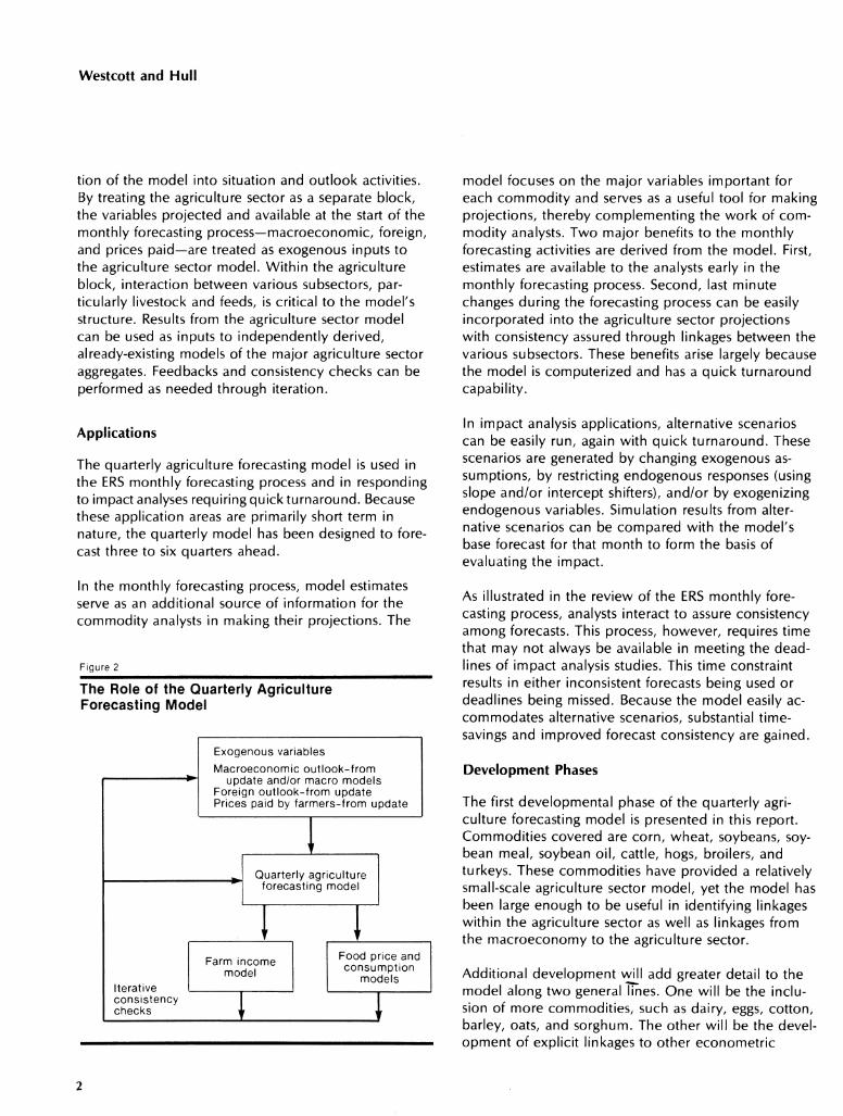
tion of the model into situation and outlook activities. By treating the agriculture sector as a separate block, the variables projected and available at the start of the monthly forecasting process—macroeconomic, foreign, and prices paid—are treated as exogenous inputs to the agriculture sector model. Within the agriculture block, interaction between various subsectors, par- ticularly livestock and feeds, is critical to the model's structure. Results from the agriculture sector model can be used as inputs to independently derived, already-existing models of the major agriculture sector aggregates. Feedbacks and consistency checks can be performed as needed through iteration.
model focuses on the major variables important for each commodity and serves as a useful tool for making projections, thereby complementing the work of com- modity analysts. Two major benefits to the monthly forecasting activities are derived from the model. First, estimates are available to the analysts early in the monthly forecasting process. Second, last minute changes during the forecasting process can be easily incorporated into the agriculture sector projections with consistency assured through linkages between the various subsectors. These benefits arise largely because the model is computerized and has a quick turnaround capability.
Applications
The quarterly agriculture forecasting model is used in the ERS monthly forecasting process and in responding to impact analyses requiring quick turnaround. Because these application areas are primarily short term in nature, the quarterly model has been designed to fore- cast three to six quarters ahead.
In the monthly forecasting process, model estimates serve as an additional source of information for the commodity analysts in making their projections. The
Figure 2
The Role of the Quarterly Agriculture Forecasting Model
Exogenous variables
Macroeconomic outlook-from update and/or nnacro nnodels
Foreign outlook-fronn update Prices paid by farnners-from update
Quarterly agriculture forecasting model
Iterative consistency checks
Farm income model
Food price and consumption
models
In impact analysis applications, alternative scenarios can be easily run, again with quick turnaround. These scenarios are generated by changing exogenous as- sumptions, by restricting endogenous responses (using slope and/or intercept shifters), and/or by exogenizing endogenous variables. Simulation results from alter- native scenarios can be compared with the model's base forecast for that month to form the basis of evaluating the impact.
As illustrated in the review of the ERS monthly fore- casting process, analysts interact to assure consistency among forecasts. This process, however, requires time that may not always be available in meeting the dead- lines of impact analysis studies. This time constraint results in either inconsistent forecasts being used or deadlines being missed. Because the model easily ac- commodates alternative scenarios, substantial time- savings and improved forecast consistency are gained.
Development Phases
The first developmental phase of the quarterly agri- culture forecasting model is presented in this report. Commodities covered are corn, wheat, soybeans, soy- bean meal, soybean oil, cattle, hogs, broilers, and turkeys. These commodities have provided a relatively small-scale agriculture sector model, yet the model has been large enough to be useful in identifying linkages within the agriculture sector as well as linkages from the macroeconomy to the agriculture sector.
Additional development will add greater detail to the model along two general lines. One will be the inclu- sion of more commodities, such as dairy, eggs, cotton, barley, oats, and sorghum. The other will be the devel- opment of explicit linkages to other econometric

A Quarterly Forecasting Model
models such as macroeconomic models and aggregate agriculture sector models for farm income, food prices, and food consumption.
Model Structure
equilibrium model with stocks derived as a residual (see fig. 5). Soybean crushing is a derived demand primarily used to supply soybean meal for feed use and export. Consequently, domestic soybean meal de- mand "drives" the soybean sector by being used to determine meal production, soybean crush, and soy- bean oil production.
The general structure used to develop the crop sub- sectors is a disequilibrium model with ending stocks clearing the market. A disequilibrium model is more appropriate for crops in a quarterly framework than in a longer run (annual) framework because, with shorter time periods, markets are more likely to be in adjust- ment rather than approximating equilibrium. Incomplete market adjustments from quarter to quarter largely reflect the lag structures in supply and demand func- tions which prevent complete adjustments in the short run. Thus, part of the ending stocks from each quarter are likely the result of incomplete market adjustments.
Figures 3 through 5 show the structures of the corn, wheat, and soybean sector models. Supply and use are determined from estimated equations for their com- ponents, price is determined using an autoregressive formulation, and ending stocks clear the market—they are the residual of supply minus use.
The soybean sector is more complex than the corn and wheat sectors because it is linked to the soybean meal and soybean oil product markets through crush- ings and prices. Each product market also uses a dis-
The soybean sector structure also provides a full quarterly supply and use balance sheet for soybeans that is not available elsewhere. Problems arise in ac- commodating the soybean and product markets because of the timing of available data. Soybean stocks data are reported for September 1, January 1, April 1, and June 1, giving uneven quarters—a 4-month quarter, a 2- month quarter, and two 3-month quarters. On the other hand, the product market data are reported on even 3-month quarters throughout their marketing years (each marketing year beginning October 1). As a result, the quarterly balance sheet for soybeans must fit the uneven quarters necessitated by the stock reporting dates, yet it must also be linked with the even quarters of the product market data. To do this, two different, though related, crush series are main- tained by the model: crush used in the soybean balance sheet is on the uneven-quarter basis; crush used for the product markets is on the even-quarter basis.
Feasibility constraints are imposed on the crop sector models in simulations to assure that market-clearing stocks are not negative. For corn and wheat, the feed
Figure 3
Corn Sector Structure
Figure 4
Wheat Sector Structure
Corn supply
Planted acres Harvested acres Yields Production Beginning stocks Innports
Ending corn stocks Privately held free stocks CGC loans Farmer-owned reserve CGC owned
Corn utilization
Feed Food and industrial Seed Alcoholic beverages Exports
XT! Corn price Farm price
Wheat supply Planted acres Harvested acres Yields Production Beginning stocks Imports
Ending wheat stocks Privately held free stocks CGC loans Farmer-owned reserve GGG owned
Wheat utilization
Feed Food Seed Exports
x: Wheat price Farm price

Westcott and Hull
demand equation is allowed to operate as long as the implied privately held free stock residual is not nega- tive. However, if the feed demand equation implies a negative privately held free stock, feed demand is set at the level that results in privately held free stocks equalling zero. A more involved and stronger constraint has been included in the soybean sector reflecting the more complex model structure and the use of an in- verse stocks-to-use ratio in the soybean price equation.
Figure 5
Soybean Sector Structure
1
Soybean supply Planted acres Han/ested acres Yields Production Beginning stocks
Soybean utilization
Crushings* - even quarters - uneven quarters
Seed, feed, and residual Exports
i
1 yK r Ending
soybean stocks Soybean price
Farm price
Meal supply Yields Production Beginning stocks
Meal utilization
Domestic use Exports
i
1 : X r
Ending meal stocks
Meal price Decatur
Oil supply Yields Production Beginning stocks
Oil utilization Domestic use Exports
i i
r X i i
Ending oil stocks Oil price Decatur
* Even-quarter crushings used for product market linkages; uneven-quarter crushings used for soybean supply and use balance sheet.
The domestic soybean meal demand equation is allowed to operate as long as the implied soybean crush does not bring ending soybean stocks below 800 million bushels on December 31, 550 million bushels on March 31, 300 million bushels on May 31, and 50 million bushels on August 31. These levels were chosen to assure ample availability of soybean supplies through the marketing year to meet crushing and ex- port demands.
An interesting aspect of the crop models is the incor- poration of annual variables into the quarterly frame- work. Production is derived in an annual framework using acres planted, acres harvested, and yields. An- nual production is then embedded into the quarterly framework. In the harvest quarter, production is added to beginning quarterly stocks and imports to derive quarterly supply; in the nonharvest quarters, produc- tion is set equal to zero.
Incorporating the annual variables into a quarterly framework has additional structural implications because of the lags involved between plantings and harvest. Production, yields, and harvested acreage all enter the crop sector models in harvest quarter. How- ever, planted acreage takes place two or three quarters earlier and is included in the model then, using quar- terly information known at that time. This differs from planting decision equations in many annual models which use variables from the previous marketing year, even though the previous marketing year is not com- pleted at the time plantings occur. To illustrate, because of the lags between plantings, harvest, and marketings, formulations of planted acreage typically include a price expectations variable to represent ex- pected returns. In "cobweb" formulations of expecta- tions, many annual models use the previous marketing year's price even though plantings occur before the previous marketing year is completed. In contrast, im- plementation of a "cobweb" formulation of planted acreage in a quarterly framework allows information known by the planting quarter, which precedes the beginning of the corresponding crop year by two or three quarters, to be used. Consequently, the price ex- pectations variable employed in the planted acreage equations is the price in the quarter immediately pre- ceding the plantings quarter.
In the cattle sector model (fig. 6), breeding herd equa- tions provide information about the capital stock from which cattle production is drawn. Constrained by the

A Quarterly Forecasting Model
size of this capital stock (the breeding herd), estimated cattle production equations for feedlot placements, marketings, and fed and nonfed steer and heifer slaughter are used to derive total commercial slaughter in an identity. Beef production estimates are derived from those slaughter estimates which are added to beginning stocks and imports to derive supply. Ending cold storage stocks are estimated. Beef consumption is derived as a residual, following the procedure used for construction of the historical consumption data. Prices for feeder steers, fed steers, cattle, and calves are estimated using supplies and derived demand factors. Product market (retail) prices are not included as part of the quarterly model because they are derived in the aggregate block in the monthly update process in a
Figure 6 „__________^_^_^.««^.^.^
Cattle Sector Structure
stage-of-processing model utilizing the farm-level prices that are estimated here.
In the hog sector model (fig. 7), the number of sows farrowing determines the size of the pig crop which is used to estimate barrow and gilt slaughter. Total hog slaughter is then derived by adding breeding herd liquidations. Supplies, utilization, and stocks of pork and prices for hogs are estimated following a structure similar to that in the cattle sector.
In the poultry sector model (fig. 8), the number of pullets placed in hatchery supply flocks constrains the size of the broiler hatch which is then used to deter- mine broiler production. Turkey production, however, is estimated directly. Supply, utilization, stocks, and prices for chickens and turkeys are each estimated fol- lowing a structure similar to that in the cattle and hog sectors.
Cattle inventories Cow mventory Steer inventory Herfer inventory Replacement heifers kept Proportion of replacement heifers
entering CO\N herd
Heifers entering cow herd
Calving rate Calf crop Cow slaughter Bull slaughter
Cattle Net placements Cattle on feed Fed cattle marketed Fed steer and heifer slaughter Nonfed steer and heifer slaughter
Total steer and heifer slaughter Commercial cattle slaughter Average dressed weight
Beef supply Production, commercial Production, farm Production, total Beginning stocks Imports
Beef utilization Total, carcass weight per capita
- carcass weight - retail weight
Ending stocks Cold storage
Prices Fed steers Cattle, farm Calves, farm Feeder steers
The livestock sector includes lags necessitated by the length of the biological production process. From breed- ing to slaughter takes about 27 months for cattle, 10 months for hogs, 3 months for broilers, and 6 months for turkeys. These temporal relationships are important for the appropriate modeling of the livestock sector and also affect the crop sector models in feed demand
Figure 7
Hog Sector Structure
Hogs Sows farrowing Pig crop Barrow and gilt slaughter
Sow slaughter Boar slaughter Hog slaughter
Pork supply Production, commercial Production, farm Production, total Beginning stocks Imports
Pork utilization
Total, carcass weight Per capita
- carcass weight - retail weight
X Ending stocks Cold storage
Prices
Barrows and gilts hogs, farm

Westcott and Hull
equations. As a consequence, expected returns and expected costs of production, represented by various lagged variables, play important roles. The lags also result in a higher amount of recursiveness in the model, which allows linkages between the crop and livestock subsectors to be made without the problems usually associated with a high degree of simultaneity.
Equation Discussion^
All stochastic equations in the quarterly agriculture forecasting model were estimated using ordinary least squares regressions with the exception of the soybean meal price equation. For that equation, a principal components regression was used because of extreme collinearity in the regressors (29). For each equation.
^Specifications and summary statistics for each equation are shown in Appendix A. Appendix B shows an alphabetized list of variable names and definitions. Endogenous variables are shown first, followed by exogenous variables.
Figure 8
Poultry Sector Structure
Broilers ruiieis piacea m naicnery suppiy TIOCKS Broiler hatch
1 r
Chicken supply
Production Beginning stocks
Chicken utilization Total Per capita
/
^ X Ending chicleen stocks Cold storage
Prices Broilers, 9-city Broilers, farm
Turkey supply Production Beginning stocks
Turkey utilization
Total Per capita
X Ending turkey stocks Cold storage
Prices Turkeys, farm
t-statistics are reported in parentheses below the parameter estimates. The coefficient of determination (R2), the root mean squared error (RMSE), and the coefficient of variation (CV) are reported along with the estimation period for each stochastic equation. The coefficient of variation and the root mean squared error are adjusted for degrees of freedom, but the coefficient of determination is unadjusted. For annual production equations in the crop sector, predicted values are calculated by using the estimated yield and harvested acres equations. The coefficient of deter- mination, the root mean squared error, and the coeffi- cient of variation for annual crop sector production equations are then derived, but these statistics are not adjusted for degrees of freedom.
Corn Sector
The corn sector in the model consists of 17 equa- tions—8 stochastic equations and 9 identities. Equa- tions for planted acreage, harvested acreage, and yields are estimated annually and, along with the pro- duction identity, are then incorporated into the quar- terly framework in the appropriate quarters. The re- maining 13 quarterly equations cover beginning stocks and total supply, total use and its major components, total and privately held ending stocks, and prices.
Acres Planted. Corn plantings primarily take place in the second quarter (April-May). However, the corn plantings equation enters the model in the first quarter because some plantings occur earlier and, as a result, the model's seed use equation for the January-March quarter depends on the planted acreage estimate. The planted acres equation makes use of the Houck-Ryan approach to incorporating price and policy variables in the model (74). This approach relies on effective price variables for payments of the crop produced and on diversion payment variables. In each case, adjustments are made to represent the commodity program require- ments in place for a given year. Houck-Ryan effective price variables and diversion payment variables are used to represent market and policy incentives for planting corn and wheat. However, soybean farm price is ap- propriately used without policy adjustments because, over the estimation period, there were no soybean acreage control programs, the soybean farm price was higher than the support rate, and there was no paid diversion program for soybeans. A further discussion of the Houck-Ryan variables used and an illustration of their construction is presented in Appendix C.

A Quarterly Forecasting Model
Competition between corn, wheat, and soybeans for cropland is represented in the corn acres planted equation by the Houck-Ryan wheat variables and the soybean price. The supply response to corn price is a modified "cobweb" framework—acres planted is a function of the Houck-Ryan effective corn price which uses first quarter corn price.
The coefficients in the acres planted equation have the expected signs. Because crop price support and supply control programs have contradictory incentives, some discussion of the sign on the Houck-Ryan effective corn price parameter in the planted acres equation may be enlightening. The effective corn price represents incentives embodied in the set-aside rate, the expected season average price for the crop being planted, and the support level. The higher the set- aside rate, the lower the effective corn price and corn plantings. The higher the expected season average price, the higher the effective corn price and corn plantings. The higher the support level, the higher the effective corn price and corn plantings. A higher sup- port level encourages greater participation by corn producers reducing corn plantings, but this reduction is offset by the cross commodity effects of additional acreage brought into the corn program from other
uses.
The coefficients of the Houck-Ryan effective wheat price and the soybean price are about the correct magnitude relative to their estimated responses in their own planted acres equations, with cross-price effects less than own-price effects. Similarly, the Houck-Ryan effective corn price coefficient is about the correct magnitude relative to its estimated response in the soy- bean acres planted equation. However, it is less than the estimated cross price effect in the wheat planted acres equation. This is likely a result of correlation be- tween the effective price for corn and the effective prices for other feed grains. The latter are not included in the model, yet their programs add to the measured cross-price effect in the wheat acreage equation while not affecting the own-price measure in the corn acre- age equation.
Acres Harvested, Yields, and Production. Corn is har vested in the fourth quarter and is related to acres planted and yields. The yield equation follows a model of Lin and Davenport with Corn Belt weather variables playing an important role (25). The 1970 dummy
variable adjusts for corn blight in the Southern States and the Corn Belt. The 1974 dummy variable adjusts for a late spring and early frost in the Lake States. An- nual corn production is derived using an identity by multiplying harvested acres by yields. Because the acres planted coefficients in the acres harvested equa- tion and the yield equation have opposite signs, the errors in those equations tend to be negatively cor- related, offsetting each other in estimates of production.
Feed Use. USDA corn feed use data were adjusted for estimating this equation because these data reflect the corn marketing year which has uneven quarters—two 3-month quarters, one 2-month quarter, and one 4-month quarter. The adjusted corn feed data used in this model were calculated by multiplying feed use in the April-May quarter by 1.5 and feed use in the June- September quarter by 0.75. Thus, all four quarters of adjusted feed use data are on a prorated, 3-month equivalent basis. This adjustment is important for flow categories to assure that the parameter estimates are not affected by the unevenness of quarters represented in the published data, thereby allowing the measure- ment of response to explanatory variables to be com- parable across quarters.
In the quarterly adjusted feed use equation, a four- quarter autoregressive term was included because of the relatively stable seasonality from year to year in corn feeding. The implied own-price elasticity is -0.46 and the implied cross-price elasticity with lagged soy- bean meal price is -0.12.^ The negative sign on the cross-price elasticity is consistent with that implied by the corn price coefficient in the soybean meal domestic demand equation.
A negative cross-price elasticity suggests that corn and soybean meal are relatively poor substitutes or possibly complements in animal feeding. Although corn contains some protein, it is fed primarily as an energy source. Soybean meal, on the other hand, is fed for protein content and is a less concentrated, more expensive source of energy than feed grains such as corn or sorghum. Previous research has generally found a posi- tive cross-price elasticity between low-protein and
^Because of the simultaneity in the model, elasticities and flexibil- ities derived from the single-equation parameter estimates are not strictly valid. Nonetheless, because of the large degree of recursive- ness in the model, the elasticities and flexibilities presented provide reasonable approximations of the full model's impact multipliers.

Westcott and Hull
high-protein feeds. These studies, however, used an- nual data and may have been reflecting that substitu- tion in aggregate animal feeding is more feasible in the long run as producers adjust the mix of animals fed.
Quarterly adjusted feed use of corn also depends on the number of cattle on feed, as well as on a two- quarter lag of farm-level livestock prices to represent expected returns to feeding. The coefficient of the former variable implies a feeding rate for cattle of 42 bushels of corn per head. This compares favorably with the feeding rate of 45 bushels of corn equivalent grain assumed for Corn Belt cost of production esti- mates (42). Estimates of corn feed use on the uneven- quarter basis are derived by unadjusting the even- quarter estimates.
Food and Industrial Use. Per capita food and industrial use of corn is a function of deflated corn and wheat prices, trend, slope shifters, and intercept shifters. It is also estimated with adjusted even-quarter basis use data. Corn use in this category has undergone signifi- cant structural shifts over the last 15 years due to the growth of high fructose corn sirup use in processed foods and soft drinks and the increased ethanol pro- duction in response to gasohol subsidies (28). The trend, slope shift, and intercept shift variables are used to represent these factors. Estimates of total corn food use on the uneven-quarter basis are derived by unad- justing the even-quarter estimates and multiplying by population.
Alcoholic Beverage Use. Per capita alcoholic beverage use of corn is positively correlated with deflated in- come. The implied income elasticity is 0.62, implying that alcoholic beverages that use corn are normal goods. The dummy variables for the second and third quarters were used to adjust for the uneven quarters in the corn marketing year.
Seed Use. Seed use reflects annual planting decisions, so the corn seed use equation has been estimated an- nually. Quarterly seed use estimates are then derived by distributing the annual estimate over the four quar- ters of the year, putting 0 in the fourth quarter, 20 per- cent in the first and third quarters, and 60 percent in the second quarter. This seed use pattern reflects the distribution of plantings: no plantings in the fourth quarter, large plantings in the second quarter, and smaller plantings in the first and third quarters. The
annual lead subscript reflects planted acreage for one year's crop taking place in the previous corn crop year, thereby using seed in the previous marketing year. The ratio of corn price to fertilizer costs (given the level of planted acres) represents an expected return of heavier seeding. The positive sign on annual trend reflects technological shifts in favor of larger seeding per acre through practices such as narrowing the distance between rows.
Stocks. Privately held free stocks are postulated to clear the market. They are calculated by subtracting use and exogenous ending stock components from supply. Total stocks are derived by adding privately held stocks to the exogenous ending stock components- stocks owned by the Commodity Credit Corporation (CCC), stocks under regular CCC loans, and stocks in the farmer-owned reserve.
Price. In the corn price equation, a one-quarter price lag is included to reflect short-term "stickiness" of prices in a quarterly framework. Price is also a func- tion of total supply and use, with use adjusted to a prorated even-quarter basis as earlier discussed for feed use of corn.
The interaction variable of acres planted with the sec- ond- and third-quarter dummy variables and the July Corn Belt weather variables represent the effects on prices of preharvest information regarding developing crops. As new information becomes available about the crop being grown, resulting expectations about the size of the upcoming harvest affect prices in the months prior to harvest. Large planted acreage and favorable weather for crop development would lead to expecta- tions of a large harvest, pushing corn prices down in the third quarter. Factors leading to expectations of a small harvest would be expected to push prices up.
The coefficients in the price equation imply that a 10-million-acre difference in planted acres causes a 3.5-cents-per-bushel difference in second- and third- quarter corn price, giving a price flexibility (evaluated at the means) of -0.12. A 1-degree difference in July Corn Belt temperature causes a 1-cent-per-bushel dif- ference in third-quarter corn prices, implying a price flexibility of 0.33. A 1-inch difference in July Corn Belt precipitation causes a 14-cent-per-bushel difference in third-quarter corn prices, implying a price flexibility of -0.25. While these flexibilities are small, these

A Quarterly Forecasting Model
variables will have additional impacts on prices in the following marketing year because of their effects on the size of the next harvest. The flexibilities shown here measure only the marginal price impacts of pre- harvest information before that information is realized in production, supply/and use.
Wheat Sector
The wheat sector in the model consists of 14 equa- tions—7 stochastic equations and 7 identities. As for corn, equations for planted acreage, harvested acre- age, and yields are estimated annually and, along with the production identity, are then incorporated into the quarterly framework in the appropriate quarters. The remaining 10 quarterly equations cover beginning stocks and total supply, total use and its major com- ponents, total and privately held ending stocks, and prices.
Acres Planted. Winter wheat plantings primarily take place in the fourth quarter (October-December), with spring wheat plantings primarily occurring in the fol- lowing April-May quarter. Since the model makes no distinction between winter and spring wheat, the acres planted equation enters the model in the fourth quar- ter. Further, since third-quarter seed use depends on the estimate of planted acres, wheat plantings are determined in the model in the third quarter.
In a specification similar to the corn plantings equa- tion, Houck-Ryan variables are used in estimating wheat acres planted.^ The competition between wheat and corn for cropland is represented by the Houck- Ryan effective corn price. As with corn, the supply response to wheat price is a modified "cobweb" framework. Acres planted is a function of the Houck- Ryan effective wheat price which uses third-quarter wheat price. Houck-Ryan diversion payment variables are not included because they did not provide a statistically significant result.
The coefficients in the acres planted equation have the expected signs. As discussed for the corn sector, the Houck-Ryan effective wheat price is about the correct magnitude relative to its estimated response in the corn acres planted equation; own-price effects exceed
^The Houck-Ryan variables are discussed more completely in the corn sector discussion and in Appendix C.
cross-price effects. The corn price coefficient in the wheat planted acres equation, however, appears high relative to its own-price effect in the corn planted acres equation. The estimated cross-price effect in the wheat equation is probably too large. Programs for other feed grains probably result in effective prices for those grains being correlated with the effective price for corn, which would upwardly bias the magnitude of the corn cross-price coefficient.
Acres Harvested, Yields, and Production. Wheat harvest takes place in the third quarter and is posi- tively correlated with acres planted. Yields are negatively correlated with acres planted and exhibit an upward trend. Excellent growing conditions in most wheat producing areas in 1971 are represented by the 1971 dummy variable. The dummy variable for 1974 adjusts for weather and disease problems. The dummy variable for 1978 adjusts for poor growing conditions in many winter wheat producing areas in late 1977 and 1978. Annual wheat production is then derived using an identity. As with corn, the negatively cor- related errors in the acres harvested and yield equa- tions, resulting from each using acres planted as an ex- planatory variable, tend to offset each other in the pro- duction estimates.
Feed and Residual Use. The wheat feed and residual use category includes a relatively large residual com- ponent that in many quarters results in negative num- bers. The largest bona fide feed use occurs in the third quarter (June-September). Consequently, the estimated equation for feed and residual use has a different func- tional form for the third quarter than for the other three quarters under the assumption that a more sys- tematic relationship could be found when the residual component is relatively smaller. The specification for first, second, and fourth quarters includes wheat prices, corn prices, and fed steer and heifer slaughter. While the inclusion of these variables is consistent with economic theory and their estimated coefficients have the expected signs, no interpretation of the magnitudes of those parameter estimates is given because the negative feed use observations affect those estimates and change the mean of the depen- dent variable needed for elasticity calculations.
The third-quarter wheat feed and residual use specification is similar to a June-September feed use study by Livezey (27). Wheat feeding depends on its own price; prices of substitute feeds, represented by

Westcott and Hull
corn and soybean meal; cattle on feed, representing a major animal group fed wheat; turkey production, as a proxy for poultry feeding (both broilers and turkeys); and a third-quarter 1976 dummy variable, adjusting for a period when a large wheat residual resulted in nega- tive third-quarter feed and residual use. The third- quarter cattle on feed coefficient implies a feeding rate for cattle of about 34 bushels per head, a reasonable estimate. The poultry variable coefficient implies wheat accounts for about 80 percent of poultry feeding re- quirements, which is somewhat large. The own-price elasticity is -6.9, the cross-price elasticity with corn is 6.0, and the cross-price elasticity with soybean meal is 1.3. The first two of these estimates are about twice as large as estimates implied by Livezey's findings, but are consistent with those estimates in supporting the argument that wheat feeding is very sensitive to rela- tive prices.
Food Use. Per capita food use of wheat is a function of deflated wheat and barley prices and seasonal and trend shifters. Food use is then derived by an identity. The small implied own-price elasticity of -0.03 and the cross-price elasticity of 0.04 likely result from the highly processed nature of most foods that use wheat so that the farm price has little effect on retail prices and final demand.
Seed Use. The seed use of wheat equation was esti- mated using observations from the second, third, and fourth quarters only because almost no planting occurs in the January-March quarter. Seed use depends on planted acreage, trend, and seasonal shifters. As with corn, the annual lead subscript reflects planted acre- age for one year's crop taking place in the previous wheat crop year, and the positive sign on annual trend reflects technological shifts in favor of larger seeding per acre. The seasonal shifters are consistent with the quarterly pattern of plantings: heaviest in the third and fourth quarters for winter wheat with smaller plantings for spring wheat in the following second quarter (April- May).
Stocks. As with corn, privately held free stocks clear the market as a residual, subtracting use and exogenous ending stock components from supply. Total stocks are derived by adding privately held stocks to those exoge- nous ending stock components.
Price. Supply, adjusted (even-quarter) use, and a one- quarter lag of wheat price are included as explanatory
variables in the wheat price equation. Two interaction variables of acres planted with the first- and second- quarter dummy variables are included to represent the effects on prices of preharvest information regarding developing crops. Their coefficients imply that a 10-million-acre difference in planted acres causes a 5.6-cents-per-bushel difference in wheat prices in the first quarter and a 10.6-cents-per-bushel difference in the second quarter, giving price flexibilities (evaluated at the means) of -0.13 and -0.26, respectively. Similar to those for corn, while these flexibilities are small, they measure only the marginal price impacts of preharvest information before that information is real- ized in the following crop year.
Soybean Sector
The soybean sector is larger than the corn and wheat sectors because it includes the soybean meal and soy- bean oil product markets, it consists of 28 equations (11 soybean, 8 soybean meal, and 9 soybean oil)—11 stochastic equations and 17 identities. As for corn and wheat, equations for planted acreage, harvested acre- age, and yields are estimated annually and, along with the production identity, are then incorporated into the quarterly framework in the appropriate quarters. Seven quarterly equations cover supply, use, stocks, and prices for soybeans. Soybean crushings and prices pro- vide the links to the soybean meal and soybean oil product markets where all 17 equations are quarterly.
Acres Planted. Soybean plantings enter the model in the second quarter. A modified "cobweb" framework is used to depict the supply response to soybean price. Acres planted is a function of expected prices, repre- sented by first-quarter soybean prices deflated by a fer- tilizer price index. The competition between corn and soybeans for cropland is represented in the soybean acres planted equation by the Houck-Ryan corn price."^ As in the corn and wheat sectors, the Houck- Ryan variable incorporates corn price and policy variables. For soybean farm prices, however, no policy adjustments are made because, over the estimation period, soybean farm prices were higher than the ef- fective support rate and there was no paid diversion program for soybeans.
"^The Houck-Ryan variables are discussed more completely in the corn sector discussion and in Appendix C.
10

A Quarterly Forecasting Model
The soybean price coefficient is about the correct order of magnitude relative to its estimated response in the corn acres planted equation. Also, the coefficient of the Houck-Ryan corn price has the expected sign and is the correct order of magnitude relative to its estimated response in the corn acres planted equation.
Acres Harvested, Yields, and Production. As with corn and v\/heat, the soybean acres harvested and yield equations both use acres planted as an ex- planatory variable which results in these equations having negatively correlated errors that tend to offset each other in production forecasts. Therefore, even though the acres-planted parameter has a weak t-statistic, it is kept in the yield relationship. The yield equation has a relatively low coefficient of determina- tion (0.75), but the 5-percent coefficient of variation in- dicates that yield estimates are quite good.
Crushings. Crush forms the basis for important linkages between the soybean market and its product markets. Two different crush series are maintained by the model. Crush used in the soybean balance sheet is on the uneven-quarter basis, while crush used for the product markets is on the even-quarter basis. Soybean crush on the even-quarter basis is derived from the soybean meal market using the identity of crush equal- ing production divided by yields. Soybean crush on an uneven-quarter basis is then derived by adjusting even- quarter crush.
Total Use and Stocks. Total soybean use is derived by adding uneven-quarter exports and seed, feed, and residual to uneven-quarter crush. Total soybean stocks then clear the market as a residual, subtracting uneven-quarter use from total supply. This results in stocks being estimated for dates corresponding to the survey dates used for historical data.
Price. The soybean price equation is estimated using a hyperbolic functional form to relate prices to ending stocks. Stocks are measured relative to a "scale of ac- tivity" indicator in the soybean sector, represented by use. This is necessary because of industry growth over the last 15 years. Further, separate hyperbolae are esti- mated for each quarter to reflect the different impor- tance of stocks through the marketing year. Plotting the resulting hyperbolic functions relating prices to the stocks-to-use ratio gives four negatively sloped curves, convex to the origin, with the hyperbolae closer to the
origin representing quarters later in the marketing year (50, 51). A separate autoregressive parameter is also estimated for each quarter in the soybean price equa- tion. Other important variables in this equation are the prices of soybean meal and soybean oil to reflect derived demand factors and the personal consumption deflator to account for inflation.
Meal Yields. Soybean meal crushing yields are ex- tremely stable and could have been left exogenous. However, validation statistics indicate a superior per- formance of this equation compared with the most likely alternative (naive "no-change" model) if yields were not endogenized. Soybean meal yields are related to the level of crush and trend. Even though the coefficient of determination is low, the coefficient of variation is extremely low. This implies that equa- tion estimates of soybean meal crushing yields are very good even though the small amount of variation pre- sent in that series is poorly explained.
Meal Production and Supplies. The soybean meal production equation is determined by domestic meal use, meal exports, and seasonal dummy variables. Accounting for roughly 75 percent of total use, domestic meal demand is the most important factor determining the level of production. With a coefficient of determination of 0.998 and a coefficient of variation of 1 percent, the model reflects the close cor- respondence and rapid adjustment of production to meal demand. Beginning stocks and supplies are determined by identities.
Domestic Meal Use. The domestic soybean meal use equation determines the derived demand for soybean crushings. It is also the major demand side link to the livestock and corn sectors and, consequently, is pos- sibly the single most important equation in the soy- bean sector. The structure of quarterly demand is "cobweb" in nature: livestock feeders cannot respond immediately to price changes, so prices of meal, corn, and livestock products are lagged one quarter. The coefficient for soybean meal price in the previous quarter implies an elasticity of -0.33, which is in the expected range based on previous research on de- mand for livestock feed. The implied cross-price elasticity between meal use and lagged corn price is -0.18. A negative cross-price elasticity suggests poor substitutability or possibly complementarity between the corresponding factors of production and is consis- tent with the relationship between these two factors found in the corn feed demand equation.
11

Westcott and Hull
The longrun effect of sows farrowing on soybean meal use is found by adding the coefficients of the two lagged variables. This implies a longrun elasticity of soybean meal demand to sows farrowing of 0.32: a 1-percent increase in sows farrowing will lead to a 0.32-percent total increase in meal use over the following two quar- ters. Using an average number of pigs saved per litter of 7.17, and adjusting the result to represent total U.S. farrowings, the sows farrowing coefficients imply about 115 pounds of soybean meal fed per hog, from farrow to finish. This compares favorably with the typical feeding operation's rate of about 130 pounds of high- protein feed, not all of which is necessarily soybean meal.
The livestock price index in the previous quarter rep- resents expected returns to feeding and indicates a strong relationship between expected product price and feed demand. Hay price is included in the meal demand equation to represent the costs of alternatives to soybean meal feeding. In the short run, decision- makers considering the placement of cattle into feed- lots can respond to relative costs of feedlot and pas- ture feeding. The implied cross-price elasticity is 0.29. The net cattle placements coefficient in the meal de- mand equation implies feeding greatly in excess of typical feedlot operations feeding. It is likely the cattle placements series is collinear with, and therefore mea- sures the effect of, other factors affecting soybean meal demand, such as environmental stress and grazing conditions.
Meal Price. In the soybean meal price equation, ex- treme collinearity between the soybean meal supply and the soybean meal use variables caused parameter estimates from ordinary least squares to have large variances and unexpected signs. Consequently, the soybean meal price equation was estimated with a principal components regression (29). This allowed para- meters on some correlated variables to change sign, although the significance of several of the parameters is still low. The reported coefficient of determination of 0.88 has been calculated using (SST-SSE)/SST, where SST is the mean corrected total sum of squares of meal prices and SSE is the sum of squared errors, it com- pares well with the coefficient of determination of 0.92 from the ordinary least squares regression.
Oil Yields and Supply. As for soybean meal, the ex- tremely stable soybean oil crushing yields could have
been left exogenous, but they are endogenized because of implications of model validation statistics. Soybean oil yields are related to the level of crush, trend, and seasonal shifters. As with soybean meal yields, the coefficient of determination is low but so is the coeffi- cient of variation, implying that equation estimates of yields are very good even though the small amount of variation present in that series is poorly explained. Pro- duction, beginning stocks, and supplies are determined by identities.
Domestic Oil Use. Domestic soybean oil demand has been estimated on a per capita basis, with the ex- planatory variables of price and disposable per capita income deflated by the personal consumption expen- ditures deflator. The seasonal nature of demand is represented by the inclusion of quarterly dummy variables. The income elasticity of 1.66 suggests that soybean oil is a luxury as a food, reflecting its use in food preparation in away-from-home establishments and in partially prepared foods sold for at-home eating. The own-price elasticity estimate is -0.09; soy- bean oil prices account for a small portion of the prices of the retail products, so demand responds little to changes in soybean oil prices.
Oil Price. As in other price equations, the soybean oil price equation includes a one-quarter lag of oil price. Soybean oil supply, soybean oil use, July temperature, and a dummy variable covering the 1973/74 soybean marketing year are also included. The July temperature coefficient implies a price flexibility of 0.14. This is consistent with similar estimates found for corn that measure the marginal price impacts of preharvest in- formation before that information is realized in the following crop year.
Cattle Sector^
Eight annual equations provide inventory information which, combined with two quarterly liquidation equa- tions, represent cow/calf operations and set breeding herd constraints on the cattle sector.
^The authors thank Richard Stillman for his collaboration on the formulation of the general framework for the livestock sector models. Much of the livestock sector presented here uses the structure of a livestock model from Stillman (34). Some parts of that framework, however, have been restructured here to meet the overall model design of the quarterly agriculture forecasting model. Also, the esti- mation periods differ from those used by Stillman.
12
A Quarterly Forecasting Model
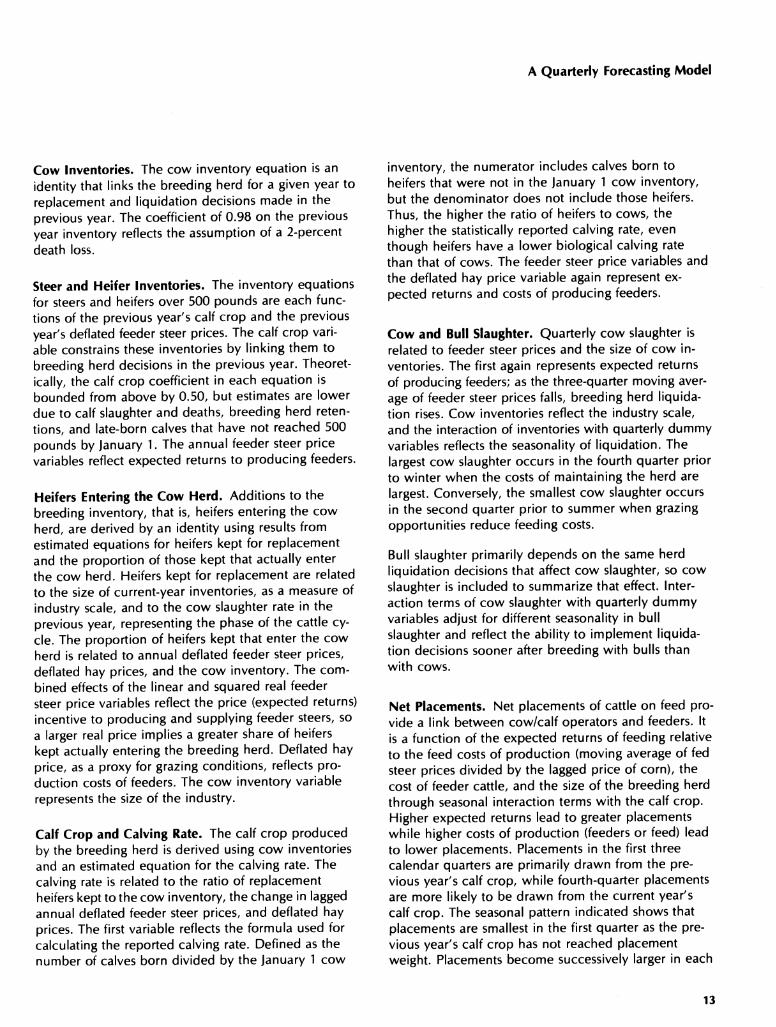
Cow Inventories. The cow inventory equation is an identity that links the breeding herd for a given year to replacement and liquidation decisions made in the previous year. The coefficient of 0.98 on the previous year inventory reflects the assumption of a 2-percent death loss.
Steer and Heifer inventories. The inventory equations for steers and heifers over 500 pounds are each func- tions of the previous year's calf crop and the previous year's deflated feeder steer prices. The calf crop vari- able constrains these inventories by linking them to breeding herd decisions in the previous year. Theoret- ically, the calf crop coefficient in each equation is bounded from above by 0.50, but estimates are lower due to calf slaughter and deaths, breeding herd reten- tions, and late-born calves that have not reached 500 pounds by January 1. The annual feeder steer price variables reflect expected returns to producing feeders.
Heifers Entering the Cow Herd. Additions to the breeding inventory, that is, heifers entering the cow herd, are derived by an identity using results from estimated equations for heifers kept for replacement and the proportion of those kept that actually enter the cow herd. Heifers kept for replacement are related to the size of current-year inventories, as a measure of industry scale, and to the cow slaughter rate in the previous year, representing the phase of the cattle cy- cle. The proportion of heifers kept that enter the cow herd is related to annual deflated feeder steer prices, deflated hay prices, and the cow inventory. The com- bined effects of the linear and squared real feeder steer price variables reflect the price (expected returns) incentive to producing and supplying feeder steers, so a larger real price implies a greater share of heifers kept actually entering the breeding herd. Deflated hay price, as a proxy for grazing conditions, reflects pro- duction costs of feeders. The cow inventory variable represents the size of the industry.
Calf Crop and Calving Rate. The calf crop produced by the breeding herd is derived using cow inventories and an estimated equation for the calving rate. The calving rate is related to the ratio of replacement heifers kept to the cow inventory, the change in lagged annual deflated feeder steer prices, and deflated hay prices. The first variable reflects the formula used for calculating the reported calving rate. Defined as the number of calves born divided by the January 1 cow
inventory, the numerator includes calves born to heifers that were not in the January 1 cow inventory, but the denominator does not include those heifers. Thus, the higher the ratio of heifers to cows, the higher the statistically reported calving rate, even though heifers have a lower biological calving rate than that of cows. The feeder steer price variables and the deflated hay price variable again represent ex- pected returns and costs of producing feeders.
Cow and Bull Slaughter. Quarterly cow slaughter is related to feeder steer prices and the size of cow in- ventories. The first again represents expected returns of producing feeders; as the three-quarter moving aver- age of feeder steer prices falls, breeding herd liquida- tion rises. Cow inventories reflect the industry scale, and the interaction of inventories with quarterly dummy variables reflects the seasonality of liquidation. The largest cow slaughter occurs in the fourth quarter prior to winter when the costs of maintaining the herd are largest. Conversely, the smallest cow slaughter occurs in the second quarter prior to summer when grazing opportunities reduce feeding costs.
Bull slaughter primarily depends on the same herd liquidation decisions that affect cow slaughter, so cow slaughter is included to summarize that effect. Inter- action terms of cow slaughter with quarterly dummy variables adjust for different seasonality in bull slaughter and reflect the ability to implement liquida- tion decisions sooner after breeding with bulls than with cows.
Net Placements. Net placements of cattle on feed pro- vide a link between cow/calf operators and feeders. It is a function of the expected returns of feeding relative to the feed costs of production (moving average of fed steer prices divided by the lagged price of corn), the cost of feeder cattle, and the size of the breeding herd through seasonal interaction terms with the calf crop. Higher expected returns lead to greater placements while higher costs of production (feeders or feed) lead to lower placements. Placements in the first three calendar quarters are primarily drawn from the pre- vious year's calf crop, while fourth-quarter placements are more likely to be drawn from the current year's calf crop. The seasonal pattern indicated shows that placements are smallest in the first quarter as the pre- vious year's calf crop has not reached placement weight. Placements become successively larger in each
13

Westcott and Hull
of the following quarters, becoming the largest in the fourth quarter when alternative feeding options are reduced.
Cattle on Feed and Fed Cattle Marketings. Cattle on feed are then derived as an identity. Fed cattle mar- ketings are a function of cattle on feed inventories plus placements with interactions with quarterly dummy variables allowing for seasonality. The seasonal pattern indicated is consistent with the seasonality in quarterly placements and feeding schedules.
Fed Steer and Heifer Slaughter. Cattle on feed inven- tories, placements, and marketings are 13-State data and must be transformed to reflect feedlot activity in the entire country. The parameter estimates represent expansion factors from marketings to slaughter, with seasonal effects again allowed through interaction terms. The seasonal slope shifters imply that fed steer and heifer slaughter outside the 13 survey States has greater seasonal distribution in the second and third quarters.
Nonfed Steer and Heifer Slaughter. Nonfed steer and heifer slaughter is inversely related to the factors that affect feedlot placement decisions and the level of fed slaughter. The more attractive feeding is—expected fed steer price high and corn price low—and the higher the level of fed slaughter, the smaller is nonfed slaughter. Also, similar to placement animals, nonfed slaughter is constrained by the annual calf crop in the previous year for the first three calendar quarters and by the annual calf crop in the current year for the fourth quarter.
Commercial Slaughter. Total commercial steer and heifer slaughter and commercial cattle slaughter are each derived by an identity.
Average Dressed Weight and Beef Supply. The moving average of fed steer prices is included in the equation for average dressed weight to represent ex- pected returns to feeding to heavier weights. The ratio of steer and heifer slaughter to cow slaughter adjusts for the weight differences between those animal groups.
A series of beef supply identities gives commercial beef production, total production, beginning cold storage stocks, and total beef supplies.
Stocks. A cold storage beef stocks equation is esti- mated rather than a beef consumption equation to re- flect the method used to collect and report the histor- ical series where consumption is derived as a residual. Ending stocks is a function of beginning stocks and im- ports, with separate quarterly coefficients allowed for each to reflect seasonality in stockholding patterns and stocks composition. The parameters on beginning stocks reflect the average duration of stocks being held. Imports represent the major source of additions to stocks.
Consumption. The procedure used for deriving the historical data is used in the model to derive, in iden- tities, civilian consumption and per capita consump- tion on both carcass and retail weight bases.
Prices. Four price equations complete the cattle sec- tor. Prices for fed steers and farm-level cattle are func- tions of fed and nonfed cattle slaughter, representing supplies, and income variables, representing derived demand factors. Diet habits tend to make demand slow in responding to income changes. This is especially true for beef which has been the traditional favorite meat in consumption, so an eight-quarter moving average of income is used. Further, the log of this moving average income variable is used to reflect diminishing marginal utility of consumption. Addi- tionally, meat demand was hypothesized to respond to both levels and changes in income, so the change in the log of the moving average of income is also includ- ed. Prices for feeder steers and farm-level calves are then related to fed steer prices to represent the de- mand for feeders, the previous year's calf crop to represent potential supplies, and lagged corn prices to represent production costs.
Hog Sector
The hog slaughter block used in the hog sector is simpler than that used for the cattle sector, but it is sufficient to support the pork supply and utilization equations. Only six equations are needed to derive total hog slaughter due to two main differences be- tween the hog and cattle industries. First, the bio- logical production lags are shorter for hogs than for cattle. Second, the hog market structure is much more vertically integrated with a large percentage of farrow- to-finish operations, while in the cattle industry, there is a greater dichotomy between breeders and feeders.
14

A Quarterly Forecasting Model
Sows Farrowing and Pig Crop. Sows farrowing is a function of expected returns to hog production repre- sented by a three-quarter moving weighted average of the seven-market hog price. The coefficient implies an elasticity of 0.44. Lagged prices for corn, the major hog feed, represent expected costs of production, with the coefficient indicating a relatively low elasticity of -0.11. Lagged sows farrowing variables are used to represent relatively stable seasonality. in farrowings from year to year and to capture longer run cyclical production decisions. The pig crop is derived by an identity.
Barrow and Gilt Slaughter. Barrow and gilt slaughter then draws on the pig crops in the two previous quar- ters, representing the 5- to 6-month farrow-to-finish production process. The seasonal dummy variables suggest that as weight gains slow in the fall and winter quarters, marketings are delayed somewhat relative to other times in the year, and are pushed into the winter and spring quarters.
Sow Slaughter and Boar Slaughter. Sow slaughter and boar slaughter represent breeding herd liquidation decisions based on biological lags, expected returns and costs, and seasonality. Sows farrowing in the pre- vious quarter is in the sow slaughter equation to repre- sent the sows available for slaughter after the new- born pigs are weaned. Expected returns are represented by the moving weighted average of hog prices while corn price represents the expected costs of produc- tion. The seasonal dummy variables indicate that sow slaughter is largest in the October-December quarter prior to winter when costs of maintaining the breeding herd rise.
Boar slaughter is related to the same factors that affect sow slaughter, so sow slaughter is included to sum- marize those factors. The positive coefficient on the in- teraction term of sow slaughter with a second quarter dummy variable reflects the ability to implement herd liquidation decisions sooner after breeding with boars than with sows and the incentive to slaughter heavy boars prior to the summer months when breeding effi- ciency is reduced. The moving weighted average of hog prices represents an additional expected returns affect in the boar slaughter decision beyond that already represented indirectly by the sow slaughter variable.
Total Hog Slaughter. Total hog slaughter is the sum of barrow and gilt slaughter, sow slaughter, and boar slaughter.
Pork Production and Supply. A structure similar to that used for the beef supply and use equations is used here for pork. A series of pork supply identities give commercial production, total production, beginning cold storage stocks, and total pork supplies.
Stocks. The equation for ending cold storage pork stocks is a function of beginning stocks and produc- tion. Similar to the beef stocks equation, separate quarterly coefficients are allowed for each indepen- dent variable to reflect seasonality in stockholding pat- terns and stocks composition. The beginning stocks parameters again reflect the average duration of stocks being held, while pork production represents potential additions to stocks.
Consumption. Civilian consumption and per capita consumption of pork on both carcass and retail weight bases are derived in identities.
Prices. Two price equations complete the hog sector. The average hog price for seven major markets is a function of pork production representing supplies, beef production representing competing meat supplies, and income variables representing derived demand factors. As in the cattle sector, the log of an eight- quarter moving average of income and the change of the log of the moving average of income are included to represent diet habits, diminishing marginal utility of consumption, and the hypothesis that both levels and changes in incomes affect demand. Prices for farm- level hogs are then related to the seven-market hog price to represent the derived demand for hogs.
Poultry Sector
The poultry sector in the model has a smaller block for breeding animals than was used in the cattle sector. Two broiler breeding flock equations are used as the basis for deriving broiler production estimates needed to support the chicken supply and use equations. Tur- key production is estimated with no explicit breeding flock constraints. This structure reflects the shorter biological production lags and the high degree of ver- tical integration in the broiler and turkey industries.
15

Westcott and Hull
Broiler Breeding Stock. Broiler pullets placed in hatchery supply flocks represent additions to the capital stock from which slaughter broilers are drawn. The four-quarter lag of placements is used because of the stable seasonality of placements from year to year. Expected feeding costs are represented by the two- quarter lag of a constructed feed cost variable, derived using a 70-percent corn and a 30-percent soybean meal feed ration. Expected returns are represented by the two-quarter lag of broiler prices. Time trend in- dicates the long-term growth in the broiler industry. The second quarter dummy variable reflects seasonally higher placements in the spring following the cold weather months when breeding flock maintenance costs are highest.
Broiler Hatch. Broilers hatched draw from the hatch- ery supply flock, represented by a weighted moving sum of placements two through four quarters earlier. The weights used are from Chavas and Johnson (6) and reflect declining productivity through the laying cycle for broiler-type chickens. The estimated coeffi- cient implies about 46 eggs are hatched per broiler- type hen in the hatchery supply flock over the laying cycle: 19 eggs two quarters after placement, 15 eggs in the following quarter, and 12 eggs four quarters after placement. Also included in the broiler hatch equation are lagged broiler prices and lagged feed prices to represent expected returns and expected production costs, respectively. Quarterly dummy variables indicate that hatch is largest in the second quarter and smallest in the fourth quarter. Trend again indicates the long- term growth in the broiler industry.
Broiler Production and Chicken Supplies. Broiler pro- duction is related to the one-quarter lag of broiler hatch to reflect the time needed to bring the birds to market weight. As before, expected returns and costs are represented by the one-quarter lags of prices for broilers and feed. Broiler industry growth is indicated by the positive time trend coefficient. Beginning cold storage stocks are derived by an identity and added to production to give total chicken supplies.
Chicken Stocks. The equation for ending chicken stocks in cold storage is a function of beginning stocks and broiler production. Separate quarterly coefficients are allowed for beginning stocks whose parameters re- flect the average duration of stocks being held. Broiler production represents potential additions to stocks.
Chicken Consumption. Similar to beef and pork, civilian chicken consumption and per capita consumption are derived in identities following the procedure used to derive the historical data.
Broiler Prices. Two price equations complete the chicken part of the poultry sector. The nine-city broiler price is a function of broiler production representing supplies, beef and pork production representing com- peting meat supplies, and income variables represent- ing derived demand factors. As in the cattle sector, the log of a moving average income variable and the change of the log of the moving average of income are included to represent habits in diets, diminishing marginal utility of consumption, and the hypothesis that both levels and changes in income affect demand. Here, however, a shorter, four-quarter moving average is used because the role of beef as the traditional favorite meat implies quicker adjustments in chicken consumption habits. Farm-level broiler prices are then related to nine-city broiler prices to represent derived demand, with a positive trend implying smaller margins that have resulted from economies of scale.
Turkey Production and Supplies. Turkey production is estimated directly without any explicit link to a sup- porting set of breeding flock equations. Turkey pro- duction is related to the two-quarter lags of turkey prices and corn prices to reflect expected returns and feeding costs. The seasonal dummy variables indicate higher production in the second half of the year when production is increased to meet larger holiday de- mand. The positive time trend coefficient indicates growth in the turkey industry. Beginning cold storage stocks are derived by an identity and added to produc- tion to give total turkey supplies.
Turkey Stocks. Similar to earlier specifications, the ending turkey stocks equation is a function of begin- ning stocks and turkey production. Separate quarterly coefficients are allowed for each independent variable to reflect seasonal stockholding patterns, which are especially important for turkeys. As for other meat stocks categories, the beginning stocks parameters reflect the average duration of stocks being held, while turkey production represents potential additions to stocks.
Turkey Consumption. Civilian turkey consumption and per capita consumption are derived in identities.
16

A Quarterly Forecasting Model
Turkey Price. A price equation completes the turkey part of the poultry sector. Farm-level turkey price is a function of the sum of beef, pork, and broiler produc- tion representing competing meat supplies and income variables representing derived demand factors. The log of a moving average income variable and the change of the log of the moving average of income are included to represent diet habits, diminishing marginal utility of consumption, and the hypothesis that both levels and changes in income affect demand. Similar to chicken, a four-quarter moving average income variable is used to reflect quicker adjustments in eating habits for poultry than for beef.
Prices Received by Farmers for Livestock
An aggregate measure of farm-level livestock prices is determined in an identity using fixed quantity weights derived from 1971-73 cash receipts from Thorp (36). The prices for eggs and milk, needed to fully represent the index of prices received by farmers for livestock, are exogenous to the model.
Model Validation
Evaluation of the model was conducted for two major purposes. First, dynamic properties were investigated to assure stability of the model. Second, validation statistics were generated from simulations designed to test the model on the basis of its intended use as a three- to six-quarter ahead forecasting tool.
In accord with the first purpose, a dynamic simulation of the model from 1975 through 1981 was performed using actual exogenous data throughout. Using the Gauss-Seidel solution method, the model converged quickly in most quarters with no quarter requiring more than 20 iterations. Validation statistics generated from this simulation (not presented here) show reason- ably good model performance. A series of additional simulations over the 1975 through 1981 interval was also performed: selected exogenous variables were im- pacted in one quarter, one year, or throughout the en- tire simulation interval, with separate simulations run for each. The model again converged quickly in all simulations with no quarter requiring more than 21 iterations. These simulations suggest that stability con- cerns are not a problem with the model.
In order to test the model on the basis of its intended use as a three- to six-quarter ahead forecasting tool.
separate dynamic model simulations were performed for each within-sample year from 1975 through 1981 (limited to this interval by data availability). This gave 28 model predictions for quarterly variables and 7 model predictions for annual variables. Two beyond- sample simulations were performed over the eight quarters and the two annual observations of 1982 and 1983. Actual exogenous data were used throughout all simulations. Validation statistics, based on these dynamic simulations of the model, are presented in table 1 and form the basis of a quantitative evaluation.
Table 1 shows summary validation statistics for each dependent variable. Relative mean absolute errors (RMAE), Theil inequality coefficients, and the relative number of turning point errors (RTPE) are presented. RMAE equals the mean absolute error (MAE) expressed as a percent of the mean of the dependent variable (y). That is, RMAE = (MAE/y) 100. The Theil inequality coefficient equals
[E [(p,-a,.,)-(a,-a,_,)]VL(a,-a,_JM ^-^
where Pt and a^ are the predicted and actual values of variables in time period t and summations are taken over all simulation periods. For annual series, k=1 to indicate the previous annual value. For quarterly series, k = 4 to indicate the four-quarter-ago value. For annual series, when t= 1, ag is set equal to the last pre- simulation value of the endogenous variable. Similarly, for quarterly series, when t < 4, actual presimulation values of the endogenous variables are used for at_4. A Theil inequality coefficient less than 1 implies superior simulation performance relative to a "naive'' forecast of no change from one year earlier (annual series) or four quarters earlier (quarterly series). The RTPEs are the number of turning point errors expressed as a per- cent of the total number of simulation observations. A turning point error occurs when
(Pt-a,_k)(a,-a,_k) < 0
with k= 1 for annual series to indicate year-to-year changes and k=4 for quarterly series to indicate changes from four quarters earlier. As for the Theil inequality coefficients, actual presimulation values of endogenous variables are used when needed (annual series, when t=1; quarterly series, when t < 4).
17

Westcott and Hull
Table 1—Quarterly agriculture forecasting model validation statistics^
Dependent variable
Relative mean absolute error (percent)^
Within sample
Beyond sample
Theil inequality
coefficient^
Within sample
Beyond sample
Relative turning point
errors (percent)'*
Within sample
Beyond sample
Corn: Annual-
Planted acres Harvested acres Yields Production
Quarterly- Beginning stocks Supply Feed Food and industrial Alcoholic beverages Seed Total use Free stocks Ending stocks Corn price, farm
Wheat: Annual-
Planted acres Harvested acres Yields Production
Quarterly- Beginning stocks Supply Feeds Food Seed Total use Free stocks Ending stocks Wheat price, farm
Soybeans: Annual-
Planted acres Harvested acres Yields Production
Quarterly- Supply Crush, even quarters Crush, uneven quarters Total use Ending stocks Soybean price, farm
See footnotes at end of table.
2.0 5.3 0.71 0.29 14 50 1.5 4.6 .72 .21 43 50 1.8 20.2 .16 .99 0 50 1.9 15.5 .15 .44 0 50
2.2 1.5 .17 .10 4 0 1.9 3.9 .20 .36 0 0 6.0 8.7 .57 1.28 18 25 3.7 10.7 .43 1.16 11 50 4.8 26.5 .62 1.17 29 88 2.6 15.5 .87 .79 0 38 3.7 5.2 .38 1.08 18 25 4.6 15.6 .30 .55 4 25 3.6 6.9 .25 .38 4 0 5.3 19.9 .42 1.01 4 38
4.7 17.4 .11 2.03 0 50 2.1 3.4 .11 .26 0 0 1.8 3.1 .47 .42 29 50 3.8 6.2 .33 .70 14 0
1.4 1.0 .13 .18 7 0 1.9 2.2 .22 .43 4 13
121.1 49.4 1.04 .90 18 13 2.2 2.1 .60 .99 32 38 1.1 20.8 .76 1.85 4 25 6.3 5.6 .66 .61 11 13 3.1 3.8 .20 .27 0 0 2.2 1.6 .19 .22 11 0 8.5 6.8 .47 1.05 18 38
4.4 8.3 .66 1.29 14 50 4.4 8.3 .64 1.28 14 50 4.4 9.6 .40 .65 0 50 6.5 17.8 .39 .85 0 0
2.8 7.0 .31 .85 4 13 4.4 9.6 .37 1.08 7 25 3.8 9.5 .37 1.20 4 38 2.1 4.9 .20 .58 0 13 4.6 11.5 .36 .85 4 13 9.6 18.0 .58 .89 21 50
Continued-
18

A Quarterly Forecasting Model
Table 1—Quarterly agriculture forecasting model validation statistics^—Continued
Relative Theil Relative
mear ) absolute inequality turning point
Dependent error (percent)^ coefficient^ errors (percent)"
variable Within Beyond Within Beyond Within Beyond
sample sample sample sample sample sample
Soybean meal: Quarterly-
Yields 0.6 0.2 0.79 0.52 29 0
Production 4.3 9.6 .37 1.07 7 25
Supply 3.9 9.3 .38 1.15 7 38
Domestic use 5,7 13.0 .55 1.32 14 38
Total use 4.2 9.4 .37 1.24 4 25
Ending stocks 16.2 26.9 .64 .72 18 25
Soybean meal price 10.4 15.1 .61 1.15 11 63
Soybean oil: Quarterly-
Yields 1.7 2.6 .63 .83 18 0
Production 4.2 11.3 .35 1.30 4 38
Supply 3.4 19.2 .32 3.55 4 63
Domestic use 4.0 3.6 .42 1.13 21 13
Total use 3.3 3.0 .33 .67 7 0
Ending stocks 10.3 49.7 .32 2.45 14 63
Soybean oil price 11.4 15.8 .48 .71 18 25
Cattle: Annual-
Cow inventory^ 2.0 3.6 .62 2.17 0 100
Steers on farms^ 3.6 2.9 1.55 1.02 14 50
Heifers on farms* 3.5 8.6 1.21 4.10 43 50
Heifers kept for cow replacement 1.5 4.3 .21 .96 0 0
Proportion of heifers kept that enter the cow herd 2.5 14.1 .28 .88 0 50
Heifers entering the cow herd 3.5 10.6 .31 .97 0 50
Annual calving rate .7 2.5 .21 1.32 0 50
Annual calf crop .7 2.5 .21 3.60 0 100
Quarterly- Cow slaughter 12.7 14.3 .63 1.98 11 75
Bull slaughter 10.1 11.7 .65 2.16 18 63
Net placements 6.0 10.7 .63 1.27 29 25
Cattle on feed 3.8 8.2 .34 1.79 29 13
Fed cattle marketed 3.7 4.4 .46 1.32 14 0
Fed steer and heifer slaughter 3.9 4.7 .46 1.15 14 0
Nonfed steer and heifer slaughter 19.8 23.2 .52 .82 7 38
Total steer and heifer slaughter 2.7 2.3 .55 1.46 21 25
Commercial cattle slaughter 4.1 2.2 .57 1.02 11 38
Average dressed weight 1.8 1.7 .54 1.21 39 25
Beef production, commercial 3.3 1.6 .62 .60 14 13
Beef production, total 3.3 1.5 .62 .59 14 13
Beginning beef stocks 1.1 9.3 .44 .39 14 0
Total beef supply 2.9 1.2 .63 .42 7 13
Ending beef stocks 12.0 11.1 .60 .44 21 0
Civilian beef consumption, carcass w eight 2.9 1.2 .62 .50 14 0
Civilian per capita beef consumption, carcass weight 2.9 1.2 .60 .65 21 25
Civilian per capita beef consumption, retail weight 2.9 1.1 .60 .64 21 25
Fed steer price 7.3 4.4 .52 1.29 18 50
Cattle price, farm 1.1 11.8 .44 3.78 25 75
Calf price, farm 11.7 25.2 .46 3.10 7 63
Feeder steer price 9.2 18.7 .46 3.01 14 50
<if»f> fnntnntp«; nt pnd of tPiblp. Continued—
19

Westcott and Hull
Table 1—Quarterly agriculture forecasting model validation statistics^—Continued
Dependent variable
Relative mean absolute error (percent)^
Within sample
Beyond sample
Hogs: Quarterly-
Sows farrowing Pig crop Barrow and gilt slaughter Sow slaughter Boar slaughter Hog slaughter Pork production, commercial Pork production, total Beginning pork stocks Total pork supply Ending pork stocks Civilian pork consumption, carcass weight Civilian per capita pork consumption, carcass weight Civilian per capita pork consumption, retail weight Barrow and gilt price Hog price, farm
Poultry: Quarterly-
Broiler pullets placed in hatchery supply flocks Broiler hatch Broiler production Beginning stocks, young chickens Total chicken supply Ending stocks, young chickens Civilian consumption, young chickens Civilian per capita consumption, young chickens Broiler price, nine-city Broiler price, farm Turkey production Beginning stocks, turkeys Total turkey supply Ending stocks, turkeys Civilian consumption, turkeys Civilian per capita consumption, turkeys Turkey price, farm
Aggregate livestock sector: Quarterly-
Prices received by farmers for livestock 4.6 4.6
Theil inequality
coefficient^
Within sample
Beyond sample
.42 1.53
Relative turning point
errors (percent)"*
Within sample
Beyond sample
3.3 14.8 0.34 1.52 14 38 3.3 14.8 .36 1.40 11 38 3.7 7.0 .36 .76 14 13 7.5 15.1 .36 .73 18 25 6.4 19.7 .39 1.03 18 38 3.6 6.3 .34 .68 11 13 3.6 6.4 .34 .71 n 13 3.6 6.3 .33 .70 11 13 5.6 6.2 .46 .35 7 13 3.2 5.9 .32 .67 11 13 8.6 10.4 .58 .55 11 25 3.5 6.1 .33 .74 7 13 3.5 6.0 .32 .72 14 13 3.5 6.0 .34 .78 11 13 8.9 11.1 .41 .61 14 0 9.0 11.1 .41 .60 14 13
4.9 13.8 .60 2.69 18 75 1.5 4.3 .29 3.11 7 63 1.7 3.0 .30 1.51 11 25
10.3 15.1 .43 .67 7 13 1.7 3.1 .31 1.65 18 25
16.0 28.3 .57 1.01 14 38 1.7 3.1 .33 1.01 11 13 1.7 3.1 .36 1.22 7 25 6.1 12.8 .51 1.26 7 75 7.3 13.4 .50 1.26 4 88 5.5 12.8 .80 2.48 21 63 9.2 10.6 .64 1.06 14 25 5.9 11.6 .76 2.10 18 63
12.2 19.6 .71 1.48 21 50 5.6 10.7 .81 1.55 25 75 5.6 10.6 .85 1.70 21 63 7.2 11.5 .61 1.41 11 63
25
'Based on dynamic simulations of the quarterly agriculture forecasting model with regard to the endogenous variables, using actual exogenous data throughout. Within-sample simulations: 1975-1981; beyond-sample simulations: 1982-1983.
''RMAE equals 100 times the mean absolute error relative to the mean of the dependent variable—(MAE/y) 100. ^The Theil inequality coefficient equals [i:[{p^-a,^\,)-{a^-a,_\J]^/L{a^-a^_^)^f^ where Pj and a, are the predicted and actual values of variables
in time period t. For annual series, k= 1 to indicate the previous annual value. For quarterly series, k = 4 to indicate the four-quarter-ago value. For annual series, when t= 1, a^^ is set equal to the last presimulation value of the endogenous variable. Similarly, for quarterly series, when t < 4, actual presimulation values of the endogenous variables are used. A Theil inequality coefficient less than 1 implies superior simulation performance relative to a "naive" (no-change) forecast.
4RTPE equals 100 times the number of turning point errors divided by the total number of simulation observations. A turning point error occurs when (p,-a,_.,,)(aj-a,_k) < 0, with k= 1 for annual series indicating year-to-year changes and k = 4 for quarterly series indicating changes from four quarters earlier. As for the Theil inequality coefficients, actual presimulation values of endogenous variables are used when needed (annual series, when t= 1; quarterly series, when t < 4).
"^Since negative values for wheat feed use occur, the mean dependent variable is artificially low. If the denominator for the relative mean absolute error is changed to the mean of the absolute value of wheat feed use, the relative mean absolute error is 77.0 percent in the within- sample simulations and 44.0 percent in the beyond-sample simulations.
^January 1 inventory statistics derived for the year following each simulation.
20

A Quarterly Forecasting Model
These three summary statistics were chosen because they represent three properties desired of forecasting models: a measure of the simulation errors, a measure of how well turning points are "caught/' and a com- parison of the econometric model with an appropriate naive model, which here, is the simple model of no change from one year earlier (annual series) or four quarters earlier (quarterly series).
Both the Theil inequality coefficient and the turning point error analyses employ the term (Pt-at_k) which is the change between the current predicted level and the actual level one year or four quarters ago. Actual levels from one year or four quarters earlier were used rather than predicted levels because the model is designed to be a short-term forecasting model where, in most applications, year ago or four-quarter-ago levels will be known. This is consistent with Theil's definition of the inequality coefficient (35, p. 28) ex- panded on later (35, p. 48) where Theil implicitly defines the predicted change as Pt-a*t_k where a*,_\, is the level of at_k known at the time the forecast is made. Since here we are forecasting four quarters ahead, a,__k will always be know and hence a*t_k equals a,_k- Also, for quarterly series, levels from four quarters earlier were used instead of levels from one quarter earlier because of the seasonality evident in most agricultural variables.
The within-sample validation statistics demonstrate that the model's performance was quite good. Most of the within-sample RMAEs are less than 10 percent, only three Theil inequality coefficients exceed 1, and the within-sample RTPEs are low for most variables.
Most variables perform well for at least two of the three forecasting properties summarized by the statistics presented here. To illustrate, with the exception of feed use of wheat, ending beef stocks, and ending tur- key stocks, all other variables with RMAEs exceeding 10 percent have low Theil inequality coefficients and RTPEs below 20 percent. The onfarm steer inventory category, which has a Theil inequality coefficient of 1.55, has a low RTPE of 14 percent and a low RMAE of 3.6 percent. Further, except for onfarm heifer inven- tories, all other variables with RTPEs exceeding 25 per- cent have Theil inequality coefficients below 1 and reasonably low RMAEs.
Feed use of corn, domestic use of soybean meal, all prices, the index of prices received by farmers for livestock, net placements of cattle on feed, cattle on
feed, and sows farrowing all perform very well in the within-sample simulations. This is particularly impor- tant because these variables provide most of the crit- ical links between the crop sector and the livestock sector. Price performance is quite good, especially since prices tend to be more volatile than the major supply and use categories. Although prices for calves, soybean meal, and soybean oil have within sample RMAEs between 10 and 12 percent, all other prices have lower RMAEs. The largest within-sample Theil in- equality coefficient for a price category is 0.61, and no price series has a within sample RTPE exceeding 25 percent.
Finally, most categories with RMAEs exceeding 10 per- cent are categories that are relatively small in magni- tude and, therefore, less important in determining overall supply and demand for each commodity. For example, nonfed steer and heifer slaughter has a 19.8-percent RMAE, but because it is a relatively small part of total steer and heifer slaughter, the latter's RMAE is only 2.7 percent. The relatively small ending stocks category for young chickens has a RMAE of 16.0 percent, yet the young chickens consumption estimates derived by using the stocks estimates have only a 1.7-percent RMAE. In the crop sector, soybean meal supply performs quite well (3.9-percent RMAE) in spite of the 16.2-percent RMAE in ending soybean meal stocks, mainly because average stocks represent only about 6 percent of total average soybean meal supply. Also, total wheat use has a RMAE of only 6.3 percent despite wheat feed use having a RMAE of 121.1 percent, partly because average feed use ac- counts for only about 6 percent of average total wheat use.
The poor performance of the wheat feed use category largely reflects the residual derivation of its historical values, so it includes feed use plus sampling and mea- surement errors from all other supply, use, and stocks categories. Further, because wheat feed use is relative- ly small, the residual derivation of this series results in negative values occurring for wheat feed use in some quarters. Consequently, the mean dependent variable used in the derivation of RMAE is artificially low. If the denominator for the relative mean absolute error is changed to the mean of the absolute value of wheat feed use, the resulting relative mean absolute error is 77.0 percent in the within-sample simulations.
The beyond-sample validation statistics are poorer, in- dicating that 1982 and 1983 were difficult to forecast.
21

Westcott and Hull
Many RMAEs are large, many Theil inequality coeffi- cients exceed 1, and many RTPEs are 50 percent or larger. However, the major aggregates—supply, total use (crops), and consumption (livestock)—perform reasonably well.
Many of the errors in the 1982 and 1983 simulations are a consequence of a few unusual circumstances. In 1982, livestock producers did not respond to favorable feed prices because high interest rates and weak con- sumer demand put them in poor cash flow positions. As a result, the model underestimated 1982 breeding herd liquidation which, in turn, caused simulation er- rors in the crop sector of the model where feed use was overestimated. Some of these effects carried over into 1983 as well. Additionally, the effects of the 1983 drought on yields and production of corn and soy- beans were underestimated by the model, adding to the 1983 simulation errors. Consequently, the poor beyond-sample validation statistics may simply reflect that 1982 and 1983 were years when the agriculture sector did not perform "as usual."
Additional Equations
Often when constructing large-scale econometric models, individual equations which have many desired structural properties and which perform well in a single equation framework are not used. This usually is because the equation performed unsatisfactorily when simulated in a multiequation framework and requires either a respecification of the equation or a more- involved restructuring of parts of the model. Nonethe- less, these equations may be useful for certain applica- tions which do not require full model simulations.
In the corn and wheat subsector models, this occurred for stocks and price equations. Appendix D presents corn and wheat equations for changes in stocks under CCC loan, for changes in stocks that are privately held, and for prices. The stocks equations are not part of the quarterly agriculture forecasting model because of the model structure being used for crops where stocks categories clear the market. The price equations are not part of the quarterly agriculture forecasting model because of problems encountered in model simulations.
Stocks Equations for Corn and Wheat
The stocks equations are specified in first-difference form and are based largely on a framework for an an-
nual model of Miller, Meyers, and Lancaster (31) which was extended to a quarterly framework by Golden and Burman {11). Although their models were estimated for CCC stocks only, the theoretical frame- work employed is generally applicable to other stocks categories.
Changes in Corn Stocks Under CCC Loan. In the corn equation for the change in stocks under CCC loan, production enters in the harvest (fourth) quarter when placement of corn under CCC loan is largest. Current prices and expectations of future prices (assumed to be a moving average of lagged prices) affect loan activity in opposite directions. Higher current prices cause decreased placements or increased redemptions, while higher expected prices cause increased placements or decreased redemptions. The implied elasticities, calcu- lated at variable means (using the level of stocks), are -0.86 for current price and 0.83 for expected price. Acting together, if prices have been falling recently, then expected prices will exceed current prices and more CCC loans will be held. Conversely, if prices have been rising recently, then current prices will ex- ceed expected prices and fewer CCC loans will be held. The loan rate is multiplied by the sum of the fourth- and first-quarter dummy variables (D4 -h D1). This follows Golden and Burman's procedure for han- dling CCC loan placements which typically occur in the first two quarters of the marketing year. Additionally, the three-quarter lag of this variable is included, representing the removal of stocks under CCC loans which have reached maturity.
The term COPLF (04+ D1 ) • DFORD • DFORE in the CCC loan equation for corn represents stocks that go directly into the farmer-owned reserve (FOR) after har- vest. The incentive to do this is related to the FOR loan rate (COPLF), which is restricted so that FOR placements displace CCC placements only in the fourth and first quarters [(D4 -H D1) = 1], only when direct FOR placements are allowed (DFORD = 1), and only after the FOR existed (DFORE = 1). The next term in the CCC loan equation for corn is the three- quarter lag of the previous term. This represents stocks which are not removed from CCC after the 9-month maturity period because they were not placed under CCC loan; instead they were placed directly into the FOR three quarters earlier. It also represents stocks which may have been temporarily placed under CCC loan but were moved to the FOR in the interim. Con-
22

A Quarterly Forecasting Model
sequently, the coefficient of this term exceeds the ab- solute value of the coefficient of the previous term.
Changes in Privately Held Corn Stocks. The equation for changes in privately held corn stocks also has pro- duction entering in the fourth quarter when harvest occurs and stocks are replenished. Lagged privately held corn stocks affect changes in current stocks in- versely—the larger the beginning stocks, the larger the removals or the smaller the net additions. Higher cur- rent prices cause more stocks to be removed or less to be added. The relatively low own-price elasticity of -0.08, again calculated using stock levels, is consis- tent with the disequilibrium hypothesis—a portion of privately held stocks is not explicitly demanded in a quarterly framework, so these stocks clear the market. The FOR loan rate is multiplied by the sum of the fourth- and first-quarter dummy variables (D4 + D1), representing the incentive to place the crop under loan during the heaviest placement quarters. In con- trast to the CGC stocks equation, no interaction term with DFORD is needed here because crop placements under CGC loan or directly into the FOR both repre- sent displacements from privately held stock positions.
Changes in Wheat Stocks Under CCC Loan. Similar to corn, the equation for changes in CCC wheat stocks includes production in the harvest quarter, current and expected prices, loan rate in the harvest and following quarters, and the three-quarter lag of the loan rate in the harvest and following quarters. The elasticities with respect to current and expected prices are -0.45 and 0.38, respectively. Similar to the privately held corn stocks equation, lagged ending GGG wheat stocks are included here. Also, a measure of interest rate subsidy, proxied by the difference between the 3-month Treasury bill rate and the GGG interest rate for wheat stocks, represents the incentive for using GGG placements for loans to improve liquidity for meeting cash flow obligations. Exports affect loan activity as redemptions rise or placements decline in order to support export demand.
Changes in Privately Held Wheat Stocks. Again similar to corn, the equation for changes in privately held wheat stocks includes production in the harvest quarter and lagged stocks. The higher the expected price, the stronger the incentive to hold stocks. The relatively small elasticity with respect to expected price of 0.13 is again consistent with the disequilibrium hypothesis where this category includes some stocks
that are not explicitly demanded in a quarterly framework, resulting instead from shortrun supply/de- mand imbalances. The 3-month Treasury bill interest rate represents the cost of holding stocks.
Alternative Price Equations for Corn and Wheat
The additional price equations for corn and wheat use a hyperbolic functional form to relate prices to stocks. Higher ending stocks in any particular quarter result in lower farm-level prices. However, the effects of stocks on prices differ through the marketing year, largely reflecting the annual nature of corn and wheat pro- duction. Large levels of stocks are necessary early in the marketing year to meet demand until the next har- vest. As the marketing year progresses and the next harvest approaches, lower stocks are sufficient to meet use requirements. Consequently, a given level of stocks later in a marketing year results in lower prices than the same level of stocks earlier in the marketing year. To represent the different effects of stocks through the year, a separate hyperbola is estimated for each quarter. This gives a family of four hyperbolic curves (fig. 9).
For both additional price equations, a free stocks definition is used which subtracts GGG-owned stocks
Figure 9
Hyperbolic Family of Curves Relating Quarterly Prices to the Stocks-to-use Ratio
Prices (P)
SO/UO
Stocks-to-use ratio (S/U)
23

Westcott and Hull
and FOR stocks from total stocks. Stocks are measured relative to the "scale of activity" in the corn and wheat industries, represented here by utilization.^ Fur- ther, lagged price is included to reflect short-term "stickiness" of prices in a quarterly framework, largely due to the lag structures in underlying supply and de- mand functions, including lagged price also allows the analysis to be conducted using nominal prices, thereby circumventing the issue of choosing an appropriate price deflator. As expected, in both additional price equations all coefficients of the inverse stocks-to-use ratios are positive.^ The largest coefficient occurs in the harvest quarter (for corn, the term with the fourth- quarter dummy variable, D4; for wheat, the term with the third-quarter dummy variable, D3), with coeffi- cients for successive quarters of the respective marketing years diminishing in size.
Lagged price also plays an important role. The auto- regressive parameter estimates imply average price ad- justment periods of about two and one-half quarters for corn and about five quarters for wheat. These esti- mates reflect the lags in underlying supply and de- mand functions that prevent instantaneous and com- plete market adjustments. For example, production decisions take a minimum of two quarters (corn and spring wheat) or three quarters (winter wheat) to materialize, representing the lag from plantings to harvest. Further, it may take up to an additional three quarters for supplies to respond if the production ad- justment decision occurs prior to the (once-a-year) plantings quarter. Similarly, demand functions have lags which contribute to the autoregressiveness in quarterly corn and wheat prices.
References
(1) Allen, George C, Earl F. Hodges, and Margaret Devers. "Livestock-Feed Relationships—National and State," SB-530. U.S. Department of Agricul- ture, Economic Research Service, June 1974.
(2) Allen, R. G. D. Mathematical Analysis For Econo- mists. New York: St. Martins Press, 1938.
(3) Arzac, Enrique R. and Maurice Wilkinson. "A Quarterly Model of United States Livestock and Feed Grain Markets and Some of its Policy Im- plications," American Journal of Agricultural Economics, Vol. 61, No. 2, May 1979, pp. 297-308.
(4) Brandow, G. E. Interrelations among Demands for Farm Products and Implications for Control of Market Supply. Pennsylvania Agricultural Experi- ment Station Statistical Bulletin 680. University Park, 1961.
(5) Butell, Robert and Abner Womack. Quarterly Feed Demand for Corn. ERS-649. U.S. Depart- ment of Agriculture, Economic Research Service, 1977. Reprinted from Feed Outlook and Situation, FdS-259, November 1975; FdS-260, February 1976; FdS-261, May 1976; FdS-262, September 1976.
(6) Chavas, jean-Paul and Stanley R. Johnson. "Supply Dynamics: The Case of U.S. Broilers and Turkeys," American journal of Agricultural Economics, Vol. 64, No. 3, August 1982, pp. 558-564.
^Utilization data have been adjusted because the corn and wheat marketing years have uneven quarters: two 3-month quarters, one 2-month quarter, and one 4-month quarter. This adjustment is done by multiplying use in the April-May quarter by 1.5 and use in the June-September quarter by 0.75. Thus, all four quarters of adjusted use data are on a prorated, 3-month equivalent basis, thereby allow- ing the "scale of activity" deflation of stocks to be comparable.
^While the hyperbolae being estimated can be expressed to show a direct relationship between prices and the stocks-to-use ratio (S/U) as shown in figure 9, the inverse of that ratio (S/U)"\ is the ap- propriate explanatory variable for use in estimation. For further discussion, see {50, 51).
(7) Cochrane, Willard W. and Mary E. Ryan. American Farm Policy, 1948-1973. Minneapolis: University of Minnesota Press, 1976.
(8) Evans, Sam. "Regional U.S. Cotton Acreage Response," Selected Cotton Marketing Topics, reprinted from the Cotton and Wool Situation, U.S. Department of Agriculture, Economics, Statistics, and Cooperatives Service, November 1978.
24

A Quarterly Forecasting Model
(9) Gadson, Kenneth E., J. Michael Price, and Larry E. Salathe. "The Food and Agricultural Policy Simulator (FAPSIM): Structural Equations and Variable Definitions/' Staff Report AGES820506. U.S. Department of Agriculture, Economic Research Service, May 1982.
(10) Gallagher, Paul, Michael Lancaster, Maury Bredahl, and Timothy J. Ryan. "The U.S. Wheat Economy in an International Setting: An Econometric Investigation," TB-1644. U.S. Department of Agriculture, Economics and Statistics Service, March 1981.
(11) Golden, Michael and Leonard Burman. "An Econometric Model of Farmers' Demand for Com- modity Credit Corporation Loans," Southern jour- nal of Agricultural Economics, Vol. 11, December 1979, pp. 47-55.
(12) Green, Robert C. "Forecasting Quarterly Grain Prices by Means of the Relation of Stocks to Use," NED working paper, U.S. Department of Agriculture, Economic Research Service, October 1983.
(13) Hargrove, Stanley H. "The Agriculture and Food Act of 1981—Description of the Major Commod- ity Programs," Peat, Marwick, Mitchell, and Co. Booklet, February 1982.
(14) Houck, James P. and Mary E. Ryan. "Supply Analysis for Corn in the United States: The Impact of Changing Government Programs," American journal of Agricultural Economics, Vol. 54, No. 2, May 1972, pp. 184-191.
(15) Hull, David B. and Paul C. Westcott. "Factors Af- fecting Quarterly Domestic Feed Demand for Corn," Feed Outlook and Situation Report. FdS-294. U.S. Department of Agriculture, Economic Research Service, September 1984, pp. 10-13.
(16) Hull, David B., Paul C. Westcott, and Roger L. Hoskin. "Factors Affecting Domestic Soybean Meal Use," Oil Crops Outlook and Situation Report. OCS-4. U.S. Department of Agriculture, Economic Research Service, February 1984, pp. 11-14.
(17) Jarvis, Lovell S. "Cattle as Capital Goods and Ran- chers as Portfolio Managers: An Application to the Argentine Cattle Sector," journal of Political Economy, Vol. 82, No. 3, May/June 1974, pp. 489-520.
(18) Johnson, James and Milton Ericksen. "Commodity Program Provisions under the Food and Agricul- ture Act of 1977," AER-389. U.S. Department of Agriculture, Economic Research Service, October 1977.
(19) Johnson, James, Richard W. Rizzi, Sara D. Short, and R. Thomas Fulton. "Provisions of the Agricul- tural and Food Act of 1981," AER-483. U.S. Department of Agriculture, Economic Research Service, 1982.
(20) Kenyon, David E. and R. S. Evans. Short-Term Soybean Acreage Projection Model Including Price and Policy Impacts, Research Division Bulletin 106, Virginia Polytechnic Institute and State University, Blacksburg, Va., September 1975.
(21) King, Gordon A. "The Demand and Price Structure for Byproduct Feeds." TB-1183. U.S. Department of Agriculture, 1958.
(22) Labys, W. Dynamic Commodity Models: Specifica- tion, Estimation, and Simulation. Lexington, Mass.: D.C. Heath and Co., 1973.
(23)
(24)
Lamm, R. McFall, Jr. "A Quarterly Econometric Model of the Agricultural Sector and Some of its Policy Implications," Staff Report AGES811118. U.S. Department of Agriculture, Economic Research Service, December 1981.
, and Paul C. Westcott. "The Effects of Changing Input Costs on Food Prices," American journal of Agricultural Economics, Vol. 63, No. 2, May 1981, pp. 187-196.
(25) Lin, William and Gregory Davenport. "Analysis of Factors Affecting Corn Yields: Projections to 1985," Feed Outlook and Situation Report. FdS-285. U.S. Department of Agriculture, Economic Research Service, May 1982, pp. 9-14.
25

Westcott and Hull
(26) Lin, William, james Johnson, and Linda Calvin. "Farm Commodity Programs—Who Participates and Who Benefits?" AER.474. U.S. Department of Agriculture, Economic Research Service, September 1981.
(27) Livezey, Janet. "Factors Affecting U.S. Wheat Feed Use," Wheat Outlook and Situation Report. WS-266. U.S. Department of Agriculture, Economic Research Service, November 1983, pp. 10-12.
(28) , "Food and Industrial Demand for Corn," Feed Outlook and Situation Report. FdS-286. U.S. Department of Agriculture, Economic Research Service, August 1982, pp. 10-12.
(29) Maddala, G. S. Econometrics, New York: McGraw-Hill Book Co., 1977.
(30) Meyers, William H. and Duane D. Hacklander. "An Econometric Approach to the Analysis of Soybean and Soybean Product Markets," Staff Report. U.S. Department of Agriculture, Economics and Statistics Service, National Economics Division, June 1979.
(31) Miller, Ronald R., William H. Meyers, and Michael A. Lancaster. "Farmers' Response to the Commodity Credit Corporation's Loan Program," Southern Journal of Agricultural Economics, Vol. 10, December 1978, pp. 157-164.
(32) Nelson, Kenneth E. "The Cattle-Beef Subsector in the United States: A Brief Overview," Staff Report AGES840106. U.S. Department of Agriculture, Economic Research Service, February 1984.
(33) OASIS Task Force. "OASIS-An Overview," Agricultural Economics Research, Vol. 30, No. 3, July 1978, pp. 1-7.
(34) Stillman, Richard P. "A Quarterly Model of the Livestock Industry," U.S. Department of Agriculture, Economic Research Service, forth- coming, 1985.
(35) Theil, Henri. Applied Economic Forecasting, Amsterdam: North-Holland Publishing Co., 1966.
(36) Thorp, Fred C. "The 1976 Revisions of Agricul- tural Price Indexes," U.S. Department of Agriculture, unpublished technical report, 1978.
(37) Todd, Richard and Terry Roe. "An Introduction to Iterative Methods for Solving Simultaneous Equation Models: Illustrations from Economics," University of Minnesota, Department of Agricul- tural and Applied Economics Staff Paper P78-11, July 1978.
(38) U.S. Department of Agriculture, Agricultural Stabilization and Conservation Service. A5CS Commodity Fact Sheet, for feed grains, wheat, and soybeans, various issues, 1976-1983.
(39) U.S. Department of Agriculture, Economic Research Service. Feed Outlook and Situation Report. Many issues.
(40) . Livestock and Meat Outlook and Situa- tion Report. Many issues.
(41) "Livestock and Meat Statistics: Supple- ment for 1982." SB-522, 1983.
(42) Livestock and Poultry Outlook and
(43)
Situation Report. Many issues.
Oil Crops Outlook and Situation Report. Many issues.
(44)
(45)
. "Policy Research Notes." Many issues.
Wheat Outlook and Situation Report. Many issues.
(46) U.S. Department of Agriculture, "USDA Updates 1983 Acreage Reduction Programs Report," Press release. May 4, 1983.
(47) Van Meir, Lawrence W. "Relationships Among Ending Stocks, Prices, and Loan Rates for Corn," Feed Outlook and Situation Report, FdS-290. U.S. Department of Agriculture, Economic Research Service, August 1983, pp. 9-13.
(48) Weiss, Michael D. "Fifty Years of U.S. Weather: Monthly Temperature and Precipitation by State and Farm Production Region, 1931-1980," Staff Report AGES820708. U.S. Department of Agri- culture, Economic Research Service, July 1982.
26

A Quarterly Forecasting Model
(49) Westcott, Paul C. "The NED Aggregation (51) . "Relationships Between Quarterly Routines/' NED Staff Report. U.S. Department of Wheat Prices and Stocks," Wheat Outlook and Agriculture, Economics and Statistics Service, Situation Report. WS-268. U.S. Department of January 1980. Agriculture, Economic Research Service, June
1984, pp. 9-13. (50) , David B. Hull, and Robert C. Green.
"Relationships between Quarterly Corn Prices (52) Westcott, Paul and Gary Lucier. "Quarterly and Stocks," Agricultural Economics Research, Agricultural Model Design," NED memorandum. Vol. 37, No. 1, Winter 1985, pp. 1-7. July 1982.
27
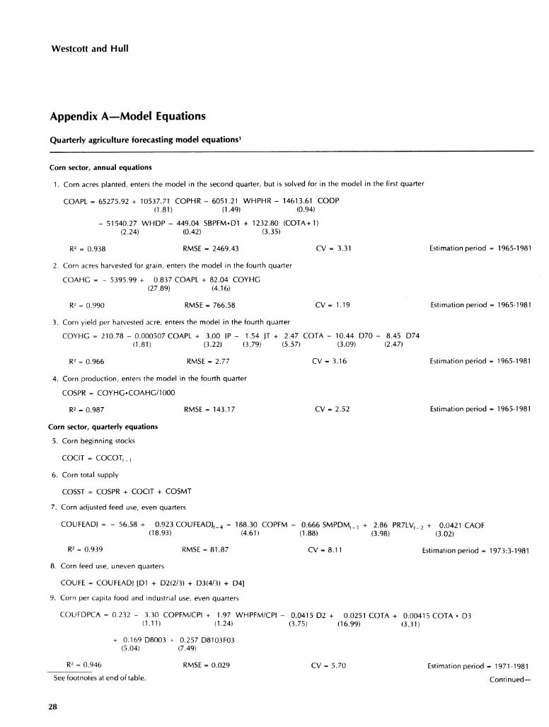
Westcott and Hull
Appendix A—Model Equations
Quarterly agriculture forecasting model equations^
Corn sector, annual equations
1. Corn acres planted, enters the model in the second quarter, but is solved for in the model in the first quarter
COAPL = 65275.92 + 10537.71 COPHR - 6051.21 WHPHR - 14613.61 CODP (1.81) (1.49) (0.94)
- 51540.27 WHDP - 449.04 SBPFM-D1 + 1232.80 (COTA+1) (2.24) (0.42) (3.35)
R2 = 0.938 RMSE = 2469.43 CV = 3.31 Estimation period = 1965-1981
2. Corn acres harvested for grain, enters the model in the fourth quarter
COAHG = - 5395.99 + 0.837 COAPL + 82.04 COYHG (27.89) (4.16)
R2 = 0.990 RMSE = 766.58 CV = 1.19 Estimation period = 1965-1981
3. Corn yield per harvested acre, enters the model in the fourth quarter
COYHG = 210.78 - 0.000507 COAPL + 3.00 jP - 1.54 jT + 2.47 COTA - 10.44 D70 - 8.45 D74 (1.81) (3.22) (3.79) (5.57) (3.09) (2.47)
R2 = 0.966 RMSE = 2.77 CV = 3.16 Estimation period = 1965-1981
4. Corn production, enters the model in the fourth quarter
COSPR = COYHG.COAHG/1000
R2 = 0.987 RMSE =» 143.17 CV - 2.52 Estimation period * 1965-1981
Corn sector, quarterly equations
5. Corn beginning stocks
COCIT = COCOTt_i
6. Corn total supply
COSST = COSPR + COCIT + COSMT
7. Corn adjusted feed use, even quarters
COUFEADj = - 56.58 + 0.923 COUFEADJt_4 - 188.30 COPFM - 0.666 SMPDMt ^ + 2.86 PR7LVt 2 + 00421 CAOF (18.93) (4.61) (1.88) (3.98) (3.02)
R' = 0.939 RMSE = 81.87 CV « 8.11 Estimation period = 1973:3-1981
8. Corn feed use, uneven quarters
COUFE = COUFEADJ [Dl + D2(2/3) + D3(4/3) -»- D4]
9. Corn per capita food and industrial use, even quarters
COUFDPCA = 0.232 - 3.30 COPFM/CPI + 1.97 WHPFM/CPI - 0.0415 D2 + 0.0251 COTA + 0.00415 COTA • D3 (1.11) (1.24) (3.75) (16.99) (3.31)
+ 0.169 D8003 f 0.257 D8103F03 (5.04) (7.49)
R' = 0.946 RMSE = 0.029 CV = 5.70 Estimation period = 1971-1981
See footnotes at end of table. Conti nued—
28

A Quarterly Forecasting Model
Quarterly agriculture forecasting model equations^—Continued
Corn sector, quarterly equations—continued
10. Corn food and industrial use, uneven quarters
COUFD = POP • COUFDPCA • [D1 + D2(2/3) + D3(4/3) + D4]
11. Corn per capita alcoholic beverage use
COUALCPC = 0.0521 + 0.00711 Y/CPI + 0.00690 D1 - 0.0122 D2 + 0.0370 D3 - 0.000413 TQ (1.44) (2.84) (5.05) (15.26) (2.40)
R2 = 0.923 RMSE = 0.0057 CV = 6.89 Estimation period = 1971-1981
12. Corn alcoholic beverage use
COUALC = COUALCPC • POP
13. Corn seed use, estimated annually by crop year; distributed over the corresponding calendar year quarters: 0 in the fourth quarter, 20 percent in the first and third quarters, 60 percent in the second quarter
COUSE = - 6.16 + 0.000242 COAPL + 110.14 COPFM • D1/PPFZ2 + 0.290 COTA (5.07) ^ (1.83) (3.87)
R2 = 0.973 RMSE = 0.61 CV = 3.69 Annual estimation period = 1964-1980 Derived quarterly estimation period = 1964:4-1981:3
14. Corn total utilization
COUUT = COUFE + COUFD + COUALC + COUSE + COUXT
15. Corn ending privately held free stocks
COCCTP = COSST - COUUT - COCCTC - CONEN - COFOR - COFOREX
16. Corn total ending stocks
COCOT = COCCTP 4- COCCTC + CONEN + COFOR + COFOREX
17. Corn price
COPFM = - 0.187 + 0.757 COPEM^.^ - 0.000265 COSST + 0.00132 COUUT [D1 + D2(3/2) + D3(3/4) + D4] (12.72) (4.29) (4.46)
- 0.00353 (COAPL/1000)-(D2 + D3) - 0.144 JP + 0.00992 JT (2.37) (2.76) (3.20)
R2 = 0.905 RMSE = 0.21 CV = 9.42 Estimation period = 1971-1981
Wheat sector, annual equations
1. Wheat acres planted, enters the model in the fourth quarter, but is solved for in the model in the third quarter
WHAPL = 48958.02 + 15819.61 WHPHR - 11073.21 COPHR (3.43) (1.52)
R2 = 0.881 RMSE = 4293.89 CV = 6.52 Estimation period = 1965-1981
See footnotes at end of table. Continued—
29

Westcott and Hull
Quarterly agriculture forecasting model equations^—Continued
Wheat sector, annual equations—continued
2. Wheat acres harvested for grain, enters the model in the third quarter
WHAHG 1727.73 + 0.916 WHAPL (28.53)
R2 = 0.982 RMSE = 1493.21
3. Wheat yield per harvested acre, enters the model in the third quarter
CV = 2.55 Estimation period = 1965-1981
Estimation period = 1965-1981
Estimation period = 1965-1981
WHYHG = 35.48 - 0.000163 WHAPL -K 0.755 WHTA -h 2.68 D71 - 3.37 D74 - 3.11 D78 (4.99) (10.03) (2.81) (3.71) (3.15)
R2 = 0.934 RMSE = 0.87 CV = 2.85
4. Wheat production, enters the model in the third quarter
WHSPR = WHYHG.WHAHG/1000
R2 = 0.985 RMSE = 97.92 CV = 6.15
Wheat sector, quarterly equations
5. Wheat beginning stocks
WHCIT = WHCOTt_i
6. Wheat total supply
WHSST = WHSPR + WHCIT + WHSMT
7. Wheat feed use
WHUFE = - 108.39 + 39.26 D1 - 6.52 D2 - 436.49 D3 + (D1 -h D2 + D4).(0.0184 STHFFQ - 13.46 WHPFM + 15.32 COPFM) (4.31) (0.72) (2.44) (2.08) (1.84) (1.19)
+ D3.(0.0338 CAOF + 0.000398 TUQ - 235.60 WHPFM + 274.72 COPFM + 0.826 SMPDM - 207.19 D7603) (2.75) (2.39) (5.54) (4.04) (3.64) (7.12)
R2 = 0.910
8. Wheat per capita food use
RMSE= 19.88 CV = 62.81 Estimation period = 1971-1981
WHUFDPC = 0.637 - 1.08 WHPFM/CPI + 2.37 BAPFM/CPI - 0.0316 Dl - 0.268 D2 + 0.185 D3 + 0.000563 TQ (1.03) (1.20) (4.38) (36.82) (25.65) (3.73)
Estimation period = 1967-1981 R2 = 0.987 RMSE = 0.020 CV = 3.04
9. Wheat food use
WHUFD = WHUFDPC.POP
10. Wheat seed use, estimated using second, third, and fourth quarters only; first quarter set exogenously in simulations; summary statistics for estimated equation reported without first quarter observations
WHUSE = - 1.04 + 0.000424 WHAPL^^^ + 0.244 WHTA - 7.57 D2 - 0.993 D3 (7.85) ^ (1.62) (8.44) (1.11)
R2 = 0.904 RMSE = 2.44 CV = 9.01 Estimation period = 1967:2-1981:4
See footnotes at end of table. Continued-
30

A Quarterly Forecasting Model
Quarterly agriculture forecasting model equations^—Continued
Wheat sector, quarterly equations—continued
11. Wheat total utilization
WHUUT = WHUFE + WHUFD + WHUSE + WHUXT
12. Wheat ending privately held free stocks
WHCCTP = WHSST - WHUUT - WHCCTC - WHNEN - WHFOR
13. Wheat total ending stocks
WHCOT = WHCCTP + WHCCTC + WHNEN + WHFOR
14. Wheat price
WHPFM = 0 229 + 0.822 WHPFM^ ^ - 0.000552 WHSST + 0.00356 WHUUT [D1 + D2(3/2) + D3(3/4) + D4] (13.50) (3.30) (3.71)
0.00563 (WHAPL/1000).D1 - 0.0106 (WHAPL/1000).D2 (2.25) (3.41)
RMSE = 0.38 CV= 12.40 R2 = 0.881
Soybean sector, annual equations
1. Soybean acres planted, enters the model in the second quarter
SBAPL = 28876.16 + 126714.0 SBPFM.D1/PPFZ2 - 1927.11 COPHR + 2381.42 (SBTA+1) (1.31) (1.05) '"-^
R2 = 0.932 RMSE == 3389.36
2. Soybean acres harvested, enters the model in the fourth quarter
SBAHB = - 1710.14 + 77.96 SBYHB + 0.971 SBAPL (2.13) (135.18)
R2 = 0.9996 RMSE = 246.67
3. Soybean yield per harvested acre, enters the model in the fourth quarter
(8.27)
CV = 6.56
CV = 0.49
SBYHB = 25.00 - 0.0000388 SBAPL + 0.327 SBTA (0.33) (1.26)
3.03 D74 + 2.81 D79 + 0.454 JP (1.86) (1.59) (1.24)
R2 = 0.754 RMSE= 1.37
4. Soybean production, enters the model in the fourth quarter
SBSPR = SBAHB.SBYHB/1000
R2 = 0.975 RMSE = 63.47
Soybean sector, quarterly equations
5. Soybean beginning stocks, uneven quarters
SBCIT = SBCOTt_,
6. Soybean total supply, uneven quarters
SBSST = SBCIT + SBSPR
CV = 5.01
CV = 4.52
Estimation period = 1971-1981
Estimation period = 1965-1981
Estimation period = 1965-1981
Estimation period - 1965-1981
Estimation period = 1965-1981
See footnotes at end of table. Continued-
31

Westcott and Hull
Quarterly agriculture forecasting model equations^—Continued
Soybean sector, quarterly equations—continued
7. Soybean crush (demand for soybean crushings derived from the meal product market), even quarters
SBUCR « SMSPR/SMYCR
8. Soybean crush, uneven quarters
SBUCRUN = SBUCR - (D2 + D3).SBUCR/3 + (D3 + D4).(SBUCR,.^ - SBUCRUN,.^) + D4.(SBUCR,_2 - SBUCRUNj_2)
9. Soybean total use, uneven quarters
SBUUTUN - SBUCRUN + SBUXTUN + SBUSFRUN
10. Soybean ending stocks, uneven quarters
SBCOT = SBSST - SBUUTUN
11. Soybean price
SBPFM » - 0.941 + 0.080 SOPDM + 0.0142 SMPDM + (0.274 D1 + 0.246 D2 + 0.249 D3 + 0.171 D4) SBPFM., (7.67) (7.93) (3.76) (3.19) (3.34) (2.28)
+ (0.128 Dl + 0.426 D2 + 0.139 D3 + 1.46 D4) [SBCOT/(SBUCR + SBUXT)]"^ + 0.00702 PCED + 0.737 D7303 (0.13) (0.65) (0.86) (0.93)
R' - 0.963 RMSE - 0.36
Soybean meal sector, quarterly equations
1. Soybean meal yield
SMYCR - 23.80 - 0.00105 SBUCR + 0.0215 SBTA (1.15) (2.35)
CV - 6.23
(2.16) (1.60)
Estimation period - 1971-1981
R2- 0.126
2. Soybean meal production
RMSE-0.17 CV - 0.70 Estimation period - 1966-1981
SMSPR » 31.30 + 0.989 SMUDT + 1.03 SMUXT - 32.42 Dl - 33.63 D2 - 61.28 D3 (1.10) (1.30) (2.46)
CV- 1.05
(51.82) (30.25)
R' = 0.998 RMSE - 54.26
3. Soybean meal beginning stocks
SMCIT = SMCOTt_i
4. Soybean meal supply, total
SMSST - SMCIT + SMSPR
5. Soybean meal domestic use
SMUDT = 124.64 - 7.45 SMPDM^.^ - 286.73 COPFM, , + 19.35 PR7LV, , (6.05) (2.08) (5.78)
+ 21.09 HAPFC + 0.216 CANPL 4- 0.120 HOSWF,.^ + 0.421 HOSWF, (2.71) (4.16) (0.70) (2.38)
Estimation period - 1971-1981
R2 = 0.886 RMSE - 266.81 CV - 6.74 Estimation period - 1973:3-1981
See footnotes at end of table. Continued—
32

A Quarterly Forecasting Model
Quarterly agriculture forecasting model equations^—Continued
Soybean meal sector, quarterly equations—continued
6. Soybean meal use, total
SMUUT = SMUDT + SMUXT
7. Soybean meal ending stocks
SMCOT = SMSST - SMUUT
8. Soybean meal price, 44-percent protein, Decatur^
SMPDM = 0.0611 + 0.000509 SMUUT - 0.00124 SMSST + 0.453 SMPDM^.^ (0.22) (0.50) (6.36)
- 1.31 SOPDMj., + 0.793 PR7LV + 133.47 D7302 + 5.59 SBPFM^.i (2.97) (3.01) (5.96) (5.44)
R2 = 0.881 RMSE = 21.34 CV = 16.02
Soybean oil sector, quarterly equations
1. Soybean oil yield
SOYCR = 10.52 - 0.000281 SBUCR + 0.0281 SBTA + 0.0523 D1 + 0.184 D2 + 0.242 D3
Estimation period - 1965-1981
(2.43) (0.78) (2.67) (3.16)
RMSE-0.19 CV=1.74 Estimation period - 1966-1981
(0.23)
R2 = 0.416
2. Soybean oil production
SOSPR = SBUCR-SOYCR
3. Soybean oil beginning stocks
SOCIT - SOCOTj_i
4. Soybean oil supply, total
SOSST = SOCIT + SOSPR
5. Soybean oil domestic use, per capita
SOUDTPC = - 3 80 - 4.57 SOPDM/PCED + 324.45 Y/POP/PCED + 1.89 D7401 - 0.207 D1 - 0.451 D2 - 0.437 D3 (1.48) (3.30) (3.19)
Estimation period = 1965-1981
(4.62) (28.27) (4.36)
R2 = 0.933 RMSE - 0.40 CV = 4.98
6. Soybean oil domestic use, total
SOUDT ^ SOUDTPC.POP
7. Soybean oil use, total
SOUUT = SOUDT + SOU XT
8. Soybean oil ending stocks
SOCOT = SOSST - SOUUT
See footnotes at end of table. Continued—
33

Westcott and Hull
Quarterly agriculture forecasting model equations^—Continued
Soybean oil sector, quarterly equations—continued
9. Soybean oil price
SOPDM - - 0.450 - 0.000563 SOSST + 0.00294 SOUUT + 0.742 SOPDMj_i + 5.751 D73MY + 0.0408 JT (0.33) (0.93) (8.96) (2.76)
R2-0.777 RMSE-3.73 CV - 16.72
Cattle sector, annual equations
1. Cow inventory, January 1
CWK - 0.980 CWKL_, - CNA/QA^.^ + HPN^.^
2. Steers over 500 pounds on farms, January 1
STG5K - 2369.22 + 3615.30 (STEPA/GNPDA) + 0.268 CVQ,. (1.36) " (3.62)
R2 - 0.526 RMSE - 670.96 CV = 4.18
3. Heifers over 500 pounds on farms, January 1
HFG5K - - 1792.35 + 3742.83 (STEPA/GNPDA) + 0.387 CVQ._, (1.70) " (6.32)
R2-0.769 RMSE-555.25 CV-3.18
4. Heifers kept for cow replacement
HFR - - 1569.58 + 0.280 CWK - 13029.59 (CWQA/CWK) (13.06) (5.63)
R2 - 0.941 RMSE - 240.92 CV « 2.26
5. Proportion of heifers kept for replacement that actually enter the cow herd
(2.34)
Estimation period - 1971-1981
Estimation period - 1967-1981
Estimation period = 1967-1981
Estimation period = 1967-1981
H FN P - 0.0289 -f- 1.95 (STEPA/GNPDA)- 2.60 (STEPA/GNPDA)^ - 0.272 (HAPFMSA/GNPDA) -h 0.010 (CWK/1000) (1.06) (1.17) (1.10) (2.50)
Estimation period = 1967-1981
+ 0.074 D74 + 0.1137 D80 (2.32) (3.54)
R'-0.815 RMSE-0.026 CV = 3.25
6. Heifers actually entering the cow herd
HFN - HFR-HFNP
7. Calving rate
CVQP - 0.760 -h 1.30 (HFR/CWK) + 0.165 [(STEPA/GNPDA), ^ - (STEPA/GNPDA), J - 0.357 (HAPFMSA/GNPDA) - 0.0351 D79 (5.42) (5.77) " '-' (9.26) (4.34)
R2 - 0.960
8. Calf crop
CVQ - CWK-CVQP
RMSE - 0.0068 CV = 0.75 Estimation period = 1967-1981
See footnotes at end of table. Continued-
34
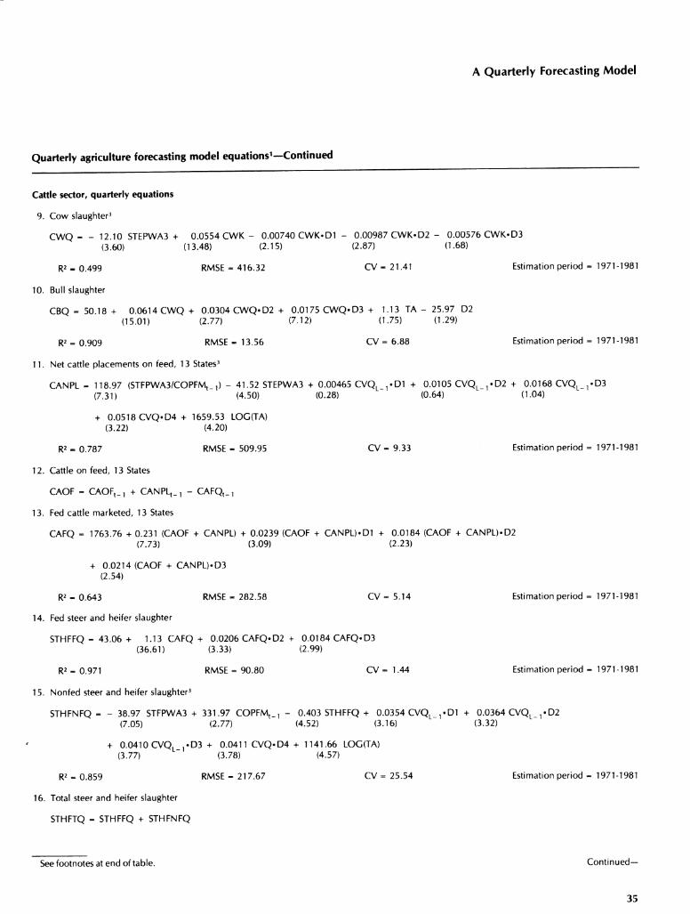
A Quarterly Forecasting Model
Quarterly agriculture forecasting model equations^—Continued
Cattle sector, quarterly equations
9. Cow slaughter^
CWQ » - 12.10 STEPWA3 + 0.0554 CWK - 0.00740 CWK-DI - 0.00987 CWK.D2 - 0.00576 CWK-D3 (3.60) (13.48) (2.15) (2.87) (1.68)
R2 - 0.499 RMSE - 416.32 CV - 21.41 Estimation period = 1971-1981
10. Bull slaughter
CBQ = 50.18 + 0.0614 CWQ + 0.0304 CWQ.D2 + 0.0175 CWQ.D3 + 1.13 TA - 25.97 D2 (15.01) (2.77) (7.12) (1.75) (1.29)
R2 = 0.909 RMSE - 13.56 CV = 6.88 Estimation period = 1971-1981
11. Net cattle placements on feed, 13 States^
CANPL - 118.97 (STFPWA3/COPFMt_i) - 41.52 STEPWA3 + 0.00465 CVQL_,«D1 + 0.0105 CVQ^.i-02 + 0.0168 CVQ^.i-03 (7.31) (4.50) (0.28) (0.64) (1.04)
+ 0.0518 CVQ.D4 + 1659.53 LOG(TA) (3.22) (4.20)
R2 » 0.787 RMSE - 509.95 CV = 9.33 Estimation period = 1971-1981
12. Cattle on feed, 13 States
CAOF = CAOFt_i + CANPL^.i - CAFQ^.,
13. Fed cattle marketed, 13 States
CAFQ = 1763.76 + 0.231 (CAOF + CANPL) + 0.0239 (CAOF + CANPL).D1 + 0.0184 (CAOF -h CANPL).D2 (7.73) (3.09) (2.23)
+ 0.0214 (CAOF -f- CANPL).D3 (2.54)
R2 = 0.643 RMSE - 282.58 CV = 5.14 Estimation period = 1971-1981
14. Fed steer and heifer slaughter
STHFFQ = 43.06 + 1.13 CAFQ + 0.0206 CAFQ.D2 + 0.0184 CAFQ.D3 (36.61) (3.33) (2.99)
R2 = 0.971 RMSE = 90.80 CV = 1.44 Estimation period = 1971-1981
15. Nonfed steer and heifer slaughter^
STHFNFQ - - 38.97 STFPWA3 + 331.97 COPEM^.^ - 0.403 STHFFQ + 0.0354 CVQ^.^.DI + 0.0364 CVQL_T.D2
(7.05) (2.77) (4.52) (3.16) (3.32)
+ 0.0410CVQ, ,.D3 4- 0.0411 CVQ.D4 -h 1141.66 LOG(TA) (3.77) " (3.78) (4.57)
R2 = 0.859 RMSE = 217.67 CV = 25.54 Estimation period = 1971-1981
16. Total steer and heifer slaughter
STHFTQ = STHFFQ + STHFNFQ
See footnotes at end of table. Continued-
35

Westcott and Hull
Quarterly agriculture forecasting model equations^—Continued
Cattle sector, quarterly equations—continued
17. Commercial cattle slaughter
CATQ = STHFTQ + CWQ + CBQ
18. Cattle, average dressed weight, commercial production
CAADW = 516.02 + 0.685 STFPWA3 + 17.216 (STHFTQ/CWQ) (6.01) (9.94)
R2 = 0.791 RMSE = 9.19 CV = 1.49 Estimation period - 1971-1981
19. Beef production, commercial
BEQC = CATQ.CAADW/1000
20. Beef production, total
BEQT = BEQC + BEQF
21. Beginning beef stocks, cold storage
BECIT = BECOT,.,
22. Total beef supply
BESST = BECIT + BEQT -f BESMT
23. Ending beef stocks, cold storage
BECOT = - 60.32 + BECIT (0.893 D1 + 0.835 D2 + 0.631 D3 + 0.783 D4) (4.53) (5.12) (4.17) (4.61)
+ BESMT (0.214 D1 + 0.180 D2 + 0.282 D3 + 0.398 D4) (1.55) (1.58) (2.37) (3.67)
R2 = 0.710 RMSE - 39.66 CV « 11.44 Estimation period - 1971-1981
24. Civilian beef consumption, carcass weight
BEUCCC - BESST - BECOT - BEUXT - BEUSH - BEUML
25. Civilian per capita beef consumption, carcass weight
BEUCCCPC « BEUCCC/POPCIV
26. Civilian per capita beef consumption, retail weight
BEUCCRPC = 0.740 BEUCCCPC
27. Fed steer price
STEP = - 100.72 - 0.00959 STHFFQ - 0.0128 STHFNFQ + 29.34 LOG(YMA8) + 537.04 YMA8LC + 2.60 D2 + 3.40 D3 (7.55) (9.81) (13.96) (2.42) (2.25) (2.96)
R2 = 0.950 RMSE = 2.95 CV = 5.93 Estimation period = 1972-1981
28. Cattle price, farm
CAPFM = - 123.66 - 0.00709 STHFFQ - 0.0164 STHFNFQ + 29.88 LOG(YMA8) +'608.30 YMA8LC + 2.35 D2 + 3.19 D3 (5.80) (13.10) (14.79) (2.86) (2.12) (2.88)
R2 = 0.960 RMSE = 2.84 CV - 6.33 Estimation period - 1972-1981
See footnotes at end of table. Continued-
36

A Quarterly Forecasting Model
Quarterly agriculture forecasting model equations^—Continued
Cattle sector, quarterly equations—continued
29. Calf price, farm
CVPFM - 93.18 - 0.00180 CVQL i + 1.50 STFP - 7.29 COPFM^_i + 2.48 D1 - 0.215 TQ (2.33) (7.99) (2.40) (1.05) (1.07)
R2 . 0.898
30. Feeder steer price
RMSE - 6.75 CV« 13.16 Estimation period = 197M981
STEP - 54.72 - 0.00109 CVQL_I + 1.24 STFP - 5.54 COPFM^.i (2.19) (11.33) (1.62)
RMSE - 4.65 CV - 9.06 Estimation period - 1971-1981 R2 - 0.931
Hog sector, quarterly equations
1. Sows farrowing, 10 States
HOSWF - - 788.76 + 23.53 HOP7MWA3 - 109.17 COPFM^_i + 0.660 HOSWEj.^ + 0.892 HOSWFj_4 - 0.533 HOSWE^.g (4.42) (1.68) (6.78) (11.83) (5.10)
R2-0.901 RMSE- 122.00 CV-5.17
2. Pig crop, 10 States
HOPGQ - HOSWF. HOPGQRAT
3. Barrow and gilt slaughter
HOBGQ - - 658.92 + 0.439 HOPGQt_i -f 0.694 HOPGQt_2 + 1268.64 D1 + 2028.89 D2 (7.60) (14.58) (4.07) (5.59)
Estimation period - 1975-1981
R2 - 0.929
4. Sow slaughter
RMSE - 685.07 CV - 3.58 Estimation period - 1974-1981
HOSWQ - 705.61 + 0.458 HOSWFj.i - 18.75 HOP7MWA3 + 133.90 COPFM - 286.17 D1 - 152.38 D2 - 232.25 D3 (6.50) (5.03) (2.69) (5.50) (2.75) (4.02)
R2 - 0.861
5. Boar slaughter
RMSE- 103.87 CV- 9.11 Estimation period - 1974-1981
HOBRQ - 71.21 + 0.0614 HOSWQ + 0.0147 HOSWQ.D2 - 2.50 HOP7MWA3 + 13.92 TA (4.56) (2.63) (5.69) (11.79)
R2-0.855 RMSE- 16.89
6. Hog slaughter
HOQ - HOBGQ + HOSWQ + HOBRQ
7. Pork production, commercial
POQC = HOQ • HOADW/1000
8. Pork production, total
POQT = POQC + POQF
CV - 8.24 Estimation period - 1971-1981
See footnotes at end of table. Continued-
37

Westcott and Hull
Quarterly agriculture forecasting model equations^—Continued
Hog sector, quarterly equations—continued
9. Beginning pork stocks, cold storage
POCIT = POCOTt_i
10. Total pork supply
ROSST = POCIT + POQT f POSMT
11. Ending pork stocks, cold storage
POCOT = - 25.46 + POCIT (0.874 D1 + 0.940 D2 + 0.550 D3 + 0.783 D4) (4.25) (5.35) (3.81) (3.55)
+ POQT (0.0215 D1 + 0.0163 D2 + 0.0191 D3 + 0.0339 D4) (1.11) (0.93) (1.08) (2.31)
R2 = 0.860 RMSE = 27.68
12. Civilian pork consumption, carcass weight
POUCCC = POSST - POCOT - POUXT - POUSH - POUML
13. Civilian per capita pork consumption, carcass weight
POUCCCPC = POUCCC/POPCIV
14. Civilian per capita pork consumption, retail weight
POUCCRPC = POUCCCPC^POCRWGT
15. Barrow and gilt price, 7 markets
CV= 10.39 Estimation period - 1971-1981
HOP7M 27.34 - 0.0238 POQT - 0.00599 BEQT + 26.11 LOG(YMA8) + 362.89 YMA8LC - 5.13 Dl - 9.48 D2 - 9.94 D3 (15.35)
R2 = 0.929
16. Hog price, farm
HOPFM = -0.0213 +
(4.39)
RMSE = 2.33
(12.45) (2.07)
CV - 5.64
(4.51) (6.97) (6.70)
Estimation period - 1972-1981
0.976 HOP7M (189.94)
0.148 D2 - 0.391 D3 (1.12) (2.95)
RMSE = 0.37 R2 = 0.999
Poultry sector, quarterly equations
1. Broiler pullets placed in hatchery supply flocks
CV- 1.01 Estimation period » 1970-1981
BRPL = 904.09 + 0.413 BRPL, (3.96)
R2 = 0.791
2. Broiler hatch
t_4 - 504.05 FGPFMj_2 + 58.56 BRP9Ct_2 + 555.35 D2 + 65.05 TQ (3.69) (2.04) (2.37) (4.35)
RMSE = 605.17 CV " 6.97 Estimation period - 1971-1981
BRH = - 33916.46 + 19.28 BRPLWS3,. (8.48)
+ 56542.23 D3 + 6185.78 TQ (4.72) (8.53)
2 + 4373.39 BRP9C,_, - 23177.01 FGPFM,_, + 80192.47 Dl + 144647.0 D2 (3.34) (3.80) (6.45) (12.32)
0.964 RMSE = 26703.49 CV = 2.95
See footnotes at end of table.
Estimation period «= 1971-1981
Continued—
38

A Quarterly Forecasting Model
Quarterly agriculture forecasting model equations'—Continued
Poultry sector, quarterly equations—continued
3. Broiler production
BRQ - - 391468.0 + 2.37 BRH,_, + 4351.13 BRP9Q_, (15.79) (2.33)
13414.07 FGPFMj_, (1.38)
+ 101577.0 Dl + 129912.0 D2 - 57060.73 D3 + 7006.39 TQ (5.03) (6.99) (2.48) (3.85)
R2 - 0.990 RMSE » 41645.09 CV = 1.77 Estimation period = 1971-1981
4. Beginning stocks, young chickens
BRCIT - BRCOT,_i
5. Total chicken supply
BRSST - BRCIT + BRQ
6. Ending stocks, young chickens
BRCOT - - 1085.26 + BRCIT (0.771 Dl + 0.875 D2 + 0.543 D3 + 0.963 D4) + 0.00175 BRQ + 10219.19 D3 (3.35) (8.68) (1.07) (7.99) (8.10)
R2 - 0.717 RMSE - 3736.52 CV = 13.28
7. Civilian consumption, young chickens
BRUCC - BRSST - BRCOT - BRUXT - BRUSH - BRUML
8. Civilian per capita consumption, young chickens
BRUCCPC - BRUCC/POPCIV/1000
9. Broiler price, 9-city
BRP9C - - 165.03 - 0.0233 (BRQ/1000) - 0.00751 BEQT - 0.00857 POQT (4.48) (4.83) (4.20)
+ 46.57 LOG(YMA4) + 143.56 YMA4LC + 2.42 D2 + 2.35 D3 (7.83) (1.17) (1.43) (1.29)
(1.91)
Estimation period = 1971-1981
R2 - 0.855
10. Broiler price, farm
RMSE - 2.66 CV = 6.37 Estimation period = 1972-1981
BRPFM - - 6.03 -I- 0.684 BRP9C - 0.139 D3 -h 0.0247 TQ (86.68) (1.52) (5.56)
R2 - 0.998
11. Turkey production
RMSE - 0.25 CV = 1.09 Estimation period = 1971-1981
TUQ - 429556.0 + 4503.30 TUPFM,_2 - 31789.13 COPFM,. (2.65) (2.21)
475734.0 Dl - 338739.0 D2 + 3218.47 TQ (28.04) (18.89) (2.92)
R2 = 0.964
12. Beginning stocks, turkeys
TUCIT « TUCOT,_i
RMSE = 45409.95 CV = 8.74 Estimation period = 1971-1981
See footnotes at end of table. Continued-
39

Westcott and Hull
Quarterly agriculture forecasting model equations^-—Continued
Poultry sector, quarterly equations-—continued
13. Total turkey supply
TUSST - TUCIT + TUQ
14. Ending stocks, turkeys
TUCOT « - 83389.40 + TUCIT (0.857 D1 + 0.921 D2 + 0.490 D3 + 0.277 D4) (5.14) (4.26) (2.97) (2.00)
+ TUQ (0.263 Dl + 0.340 D2 + 0.567 D3 + 0.255 D4) (2.74) (3.77) (7.91) (2.85)
R2 - 0.943 RMSE - 30457.75 CV - 12.04 Estimation period - 1971-1981
15. Civilian consumption, turkeys
TUUCC = TUSST - TUCOT - TUUXT - TUUSH - TUUML
16. Civilian per capita consumption, turkeys
TUUCCPC - TUUCC/POPCIV/1000
17. Turkey price, farm
TUPFM - - 84.40 - 0.00594 OTHERTUQT + 25.84 LOG(YMA4) + 357.85 YMA4LC - 4.23 Dl - 6.04 D2 - 5.47 D3 (2.78) (5.27) (2.09) (2.35) (3.17) (2.63)
R2 = 0.757 RMSE = 3.73 CV - 10.72 Estimation period = 1972-1981
Aggregate livestock sector variable, quarterly equation
1. Prices received by farmers for livestock
PR7LV - [0.666((480 CAPFM + 37 CVPFM + 212 HOPFM)/24442.1)
+ 0.135((56.69 EGPFM + 23.83 TUPFM + 111.11 BRPFM)/4768.3)
+ 0.199((1120MIPFM)/7156.8)] (399.16)(0.20772)
'"L" subscripts on variables denote annual lags, "t" subscripts denote quarterly lags. No subscript on variables denotes current period observations (year or quarter, as appropriate).
^Estimates of the soybean meal price equation result from a principal components regression undertaken to address extreme collinearity in the regressors. R-^ is derived using (SST - SSE)/SST, where SST is the mean corrected total sum of squares of meal prices and SSE is the sum of squared errors.
Cattle sector equations 9, 11, and 15 were estimated with intercepts constrained to equal zero. The resulting bias and systematic errors were not statistically significant.
40

A Quarterly Forecasting Model
Appendix B—Variable Definitions
Quarterly agriculture forecasting model variable definitions
Variables Definition Units
Endogenous
BECIT BECOT BEQC BEQT BESST BEUCCC BEUCCCPC BEUCCRPC BRCIT BRCOT BRH BRPFM BRPL BRPLWS3 BRP9C BRQ BRSST BRUCC BRUCCPC CAADW CAFQ CAN PL CAOF CAPFM CATQ CBQ COAHG COAPL COCCTP COCIT COCOT COPFM COSPR COSST COUALC COUALCPC COUFD COUFDPCA COUFE COUFEADj COUSE COU UT COYHG CVPFM CVQ CVQP CWK CWQ CWQA FGPFM HFG5K HFN HFNP HFR HOBGQ
Beginning beef stocks, cold storage Ending beef stocks, cold storage Beef production, commercial Beef production, total Total beef supply Civilian beef consumption, carcass weight Civilian per capita beef consumption, carcass weight Civilian per capita beef consumption, retail weight Beginning stocks, young chickens Ending stocks, young chickens Broiler hatch Broiler price, farm Broiler pullets placed in hatchery supply flocks Moving weighted sum of BRPL* Broiler price, nine-city Broiler production Total chicken supply Civilian consumption, young chickens Civilian per capita consumption, young chickens Cattle, average dressed weight, commercial production Fed cattle marketed, 13 States Net cattle placements on ieed, 13 States Cattle on feed, 13 States Cattle price, farm Commercial cattle slaughter Bull slaughter Acres harvested for grain, corn Acres planted, corn Ending privately held free stocks, corn Beginning stocks, corn Ending stocks, corn Farm price, corn Production, corn Total supply, corn Alcoholic beverage use, corn Per capita alcoholic beverage use, corn Food and industrial use, corn, uneven quarters Per capita food and industrial use, corn, even quarters* Feed use, corn, uneven quarters Adjusted feed use, corn, even quarters* Seed use, corn Total utilization, corn Yield per harvested acre, corn Calf price, farm Annual calf crop Annual calving rate Cow inventory, January 1 Cow slaughter Annual cow slaughter* Feed price—weighted average of corn price and soybean meal price* Heifers over 500 pounds on farms, January 1 Heifers actually entering the cow herd Proportion of heifers kept for replacement that actually enter the cow herd Heifers kept for cow replacement Barrow and gilt slaughter
Mil. lbs. Mil. lbs. Mil. lbs. Mil. lbs. Mil. lbs. Mil. lbs. Pounds/person Pounds/person 1,000 lbs. 1,000 lbs. 1,000 chicks $/cwt 1,000 pullets 1,000 pullets $/cwt 1,000 lbs. 1,000 lbs. 1,000 lbs. Pounds/person Pounds 1,000 head 1,000 head 1,000 head $/cwt 1,000 head 1,000 head 1,000 acres 1,000 acres Mil. bu. Mil. bu. Mil. bu. $/bu. Mil. bu. Mil. bu. Mil. bu. Bu./person Mil. bu. Bu./person Mil. bu. Mil. bu. Mil. bu. Mil. bu. Bu./acre $/cwt 1,000 head Proportion 1,000 head 1,000 head 1,000 head $/cwt 1,000 head 1,000 head Proportion 1,000 head 1,000 head
*See arithmetic expressions for constructed variables at end of table. Continued-
41

Westcott and Hull
Quarterly agriculture forecasting model variable definitions—Continued
Variables Definition Units
Endogenous, continued
HOBRQ HOPFM HOPGQ HOP7M HOP7MWA3 HOQ HOSWF HOSWQ OTHERPOQT OTHERTUQT POCIT POCOT POQC POQT POSST POUCCC POUCCCPC POUCCRPC PR7LV SBAHB SBAPL SBCIT SBCOT SBPFM SBSPR SBSST SBUCR SBUCRUN SBUUTUN SBYHB SMCIT SMCOT SMPDM SMSPR SMSST SMUDT SMUUT SMYCR SOCIT SOCOT SOPDM SOSPR SOSST SOUDT SOUDTPC SOUUT SOYCR STEP STEPA STEPWA3 STEP STFPWA3 STG5K STHFFQ STHFNFQ STHFTQ TUCIT
Boar slaughter Hog price, farm Pig crop, 10 States Barrow and gilt price, seven markets Moving weighted average of HOP7M* Hog slaughter Sows farrowing, 10 States Sow slaughter Meat and poultry production less pork production* Meat and poultry production less turkey production* Beginning pork stocks, cold storage Ending pork stocks, cold storage Pork production, commercial Pork production, total Total pork supply Civilian pork consumption, carcass weight Civilian per capita pork consumption, carcass weight Civilian per capita pork consumption, retail weight Livestock price index Acres harvested, soybeans Acres planted, soybeans Beginning stocks, soybeans Ending stocks, soybeans Farm price, soybeans Production, soybeans Total supply, soybeans Soybean crush, even quarters Soybean crush, uneven quarters Total use, soybeans, uneven quarters Yield per harvested acre, soybeans Beginning stocks, soybean meal Ending stocks, soybean meal Soybean meal price, Decatur, 44-percent protein Production, soybean meal Total supply, soybean meal Domestic use, soybean meal Total use, soybean meal Crushing yields, soybean meal Beginning stocks, soybean oil Ending stocks, soybean oil Soybean oil price Production, soybean oil Total supply, soybean oil Total domestic use, soybean oil Per capita domestic use, soybean oil Total use, soybean oil Crushing yields, soybean oil Feeder steer price Feeder steer price, annual* Moving weighted average of STEP* Fed steer price Moving weighted average of STEP* Steers over 500 pounds on farms, January 1 Fed steer and heifer slaughter Nonfed steer and heifer slaughter Total steer and heifer slaughter Beginning stocks, turkeys
Mil. Mil. Mil. Mil.
1,000 head $/cwt 1,000 head $/cwt $/cwt 1,000 head 1,000 head 1,000 head Mil. lbs. Mil. lbs. Mil. lbs. Mil. lbs.
lbs. lbs. lbs. lbs.
Pounds/person Pounds/person 1977 = 100 1,000 acres 1,000 acres Mil. bu. Mil. bu. $/bu. Mil. bu. Mil. bu. Mil. bu. Mil. bu. Mil. bu. Bu./acre 1,000 tons 1,000 tons $/ton 1,000 tons 1,000 tons 1,000 tons 1,000 tons tons/1,000 bu. Mil. lbs. Mil. lbs. Cents/lb. Mil. lbs. Mil. lbs. Mil. lbs. Pounds/person Mil. lbs. Lbs./bu. $/cwt $/cwt $/cwt $/cwt $/cwt 1,000 head 1,000 head 1,000 head 1,000 head 1,000 lbs.
See footnotes at end of table. Continued-
42
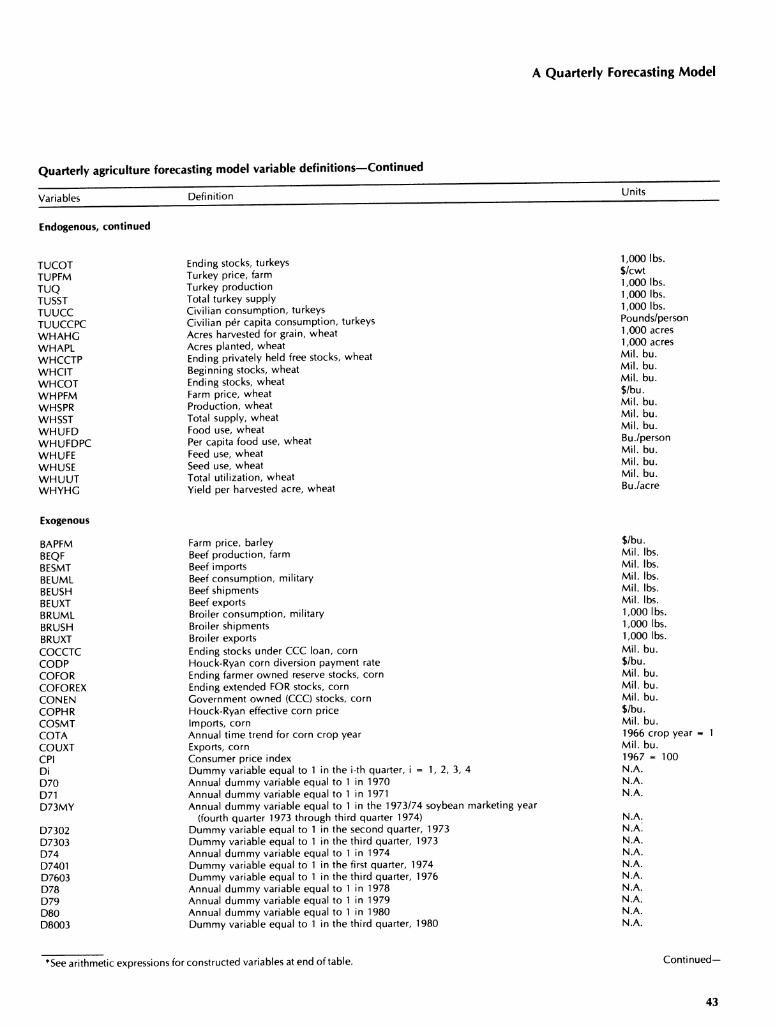
A Quarterly Forecasting Model
Quarterly agriculture forecasting model variable definitions—Continued
Variables
Endogenous, continued
Definition Units
TUCOT TUPFM TUQ TUSST TUUCC TUUCCPC WHAHG WHAPL WHCCTP WHCIT WHCOT WHPFM WHSPR WHSST WHUFD WHUFDPC WHUFE WHUSE WHUUT WHYHG
Ending stocks, turkeys Turkey price, farm Turkey production Total turkey supply Civilian consumption, turkeys Civilian per capita consumption, turkeys Acres harvested for grain, wheat Acres planted, wheat Ending privately held free stocks, wheat Beginning stocks, wheat Ending stocks, wheat Farm price, wheat Production, wheat Total supply, wheat Food use, wheat Per capita food use, wheat Feed use, wheat Seed use, wheat Total utilization, wheat Yield per harvested acre, wheat
1,000 lbs. $/cwt 1,000 lbs. 1,000 lbs. 1,000 lbs. Pounds/person 1,000 acres 1,000 acres Mil. bu. Mil. bu. Mil. bu. $/bu. Mil. bu. Mil. bu. Mil. bu. Bu./person Mil. bu. Mil. bu. Mil. bu. Bu./acre
Exogenous
BAPFM BEQF BESMT BEUML BEUSH BEUXT BRUML BRUSH BRUXT COCCTC CODP COFOR COFOREX CONEN COPHR COSMT COTA COUXT CPI Di D70 D71 D73MY
D7302 D7303 D74 D7401 D7603 D78 D79 D80 D8003
Farm price, barley Beef production, farm Beef imports Beef consumption, military Beef shipments Beef exports Broiler consumption, military Broiler shipments Broiler exports Ending stocks under CCC loan, corn Houck-Ryan corn diversion payment rate Ending farmer owned reserve stocks, corn Ending extended FOR stocks, corn Government owned (CCC) stocks, corn Houck-Ryan effective corn price Imports, corn Annual time trend for corn crop year Exports, corn Consumer price index Dummy variable equal to 1 in the i-th quarter, i = 1, 2, 3, 4 Annual dummy variable equal to 1 in 1970 Annual dummy variable equal to 1 in 1971 Annual dummy variable equal to 1 in the 1973/74 soybean marketing year
(fourth quarter 1973 through third quarter 1974) Dummy variable equal to 1 in the second quarter, 1973 Dummy variable equal to 1 in the third quarter, 1973 Annual dummy variable equal to 1 in 1974 Dummy variable equal to 1 in the first quarter, 1974 Dummy variable equal to 1 in the third quarter, 1976 Annual dummy variable equal to 1 in 1978 Annual dummy variable equal to 1 in 1979 Annual dummy variable equal to 1 in 1980 Dummy variable equal to 1 in the third quarter, 1980
*See arithmetic expressions for constructed variables at end of table.
$/b j.
Mil. lbs. Mil lbs. Mil lbs. Mil lbs. Mil lbs. 1,000 lbs. 1,000 lbs. 1,000 lbs. Mil. bu. $/bu. Mil. bu. Mil. bu. Mil. bu. $/bu. Mil. bu. 1966 crop year - 1 Mil. bu. 1967 - 100 N.A. N.A. N.A.
N.A. N.A. N.A. N.A. N.A. N.A. N.A. N.A. N.A. N.A.
Continued
43

Westcott and Hull
Quarterly agriculture forecasting model variable definitions—Continued
Variables
Exogenous, continued
Definition Units
D8103F03 EGPFM GNPDA HAPFC HAPFMSA HOADW HOPGQRAT JP JT MIPFM PCED POCRWGT POP POPCIV POQF POSMT POUML POUSH POUXT PPFZ2 SBTA SBUSFRUN SBUXT SBUXTUN SMUXT SOUXT TA TQ TUUML TUUSH TUUXT WHCCTC WHDP WHFOR WHNEN WHPHR WHSMT WHTA WHUXT Y YMA4 YMA4LC YMA8 YMA8LC
Dummy variable equal to 1 in all third quarters beginning in 1981 Egg price, farm GNP deflator, annual Hay price Hay price, annual, season average Hogs, average dressed weight, commercial production Pigs saved per litter, 10 States July precipitation. Corn Belt July temperature. Corn Belt Milk price, farm Personal consumption expenditures deflator Pork, carcass-to-retail weight conversion factor Total U.S. population Civilian population Pork production, farm Pork imports Pork consumption, military Pork shipments Pork exports Fertilizer price index, second quarter Annual time trend for soybean crop year Soybean feed and residual, uneven quarters Soybean exports, even quarters Soybean exports, uneven quarters Soybean meal exports Soybean oil exports Annual time trend Quarterly time trend Turkey consumption, military Turkey shipments Turkey exports Ending stocks under CCC loan, wheat Houck-Ryan wheat diversion payment rate Ending farmer owned reserve stocks, wheat Government owned (CCC) stocks, wheat Houck-Ryan effective wheat price Imports, wheat Annual time trend for wheat crop year Exports, wheat Personal disposable income, nominal Four quarter moving average of income* Change in the log of YMA4 Eight quarter moving average of income* Change'in the log of YMA8
N.A. = Not applicable. *Arithmetic expressions:
BRPLWS3 = BRPL + 0.80 BRPL^.i + 0.61 BRPLt_2 COUFDPCA = COUFD [Dl + D'2{3/2) + D3(3/4) + D4]/POP COUFEADJ = COUFE [Dl + D2{3/2) + D3(3/4) + D4] CWQA = D4 (CWQ + CWQ,,, + CWQ, 2 + CWQ, 3) FGPFM « 0.70 (COPFM/0,56) + 0.30 (SMPDM/20) HOP7MWA3 = (3.0 HOP/M,., + 2.0 HOPJM, j + HOP7M, ^)/6 OTHERPOQT = BEQT + BRQ/1000 + TUQ/1000 OTHERTUQT = BEQT + POQT + BRQ/1000 STEPA - D4 (STEP + STEP,., + STEP, 2 + STEP, 3) STEPWA3 = (3.0 STEP,_, + 2.0 STEP,.2 + STEP, STFPWA3 = (3.0 STEP,, + 2.0 STFR_, + STEP, t-2
7
.■i)l6
.3)/6
N.A. $/cwt 1972 == 100 $/ton $/ton Pounds Number Inches Degrees (F) $/cwt 1972 = 100 Proportion Millions Millions Mil. lbs. Mil. lbs. Mil. lbs. Mil. lbs. Mil. lbs. 1977 = 100 1966 crop year = 1 Mil. bu. Mil. bu. Mil. bu. 1,000 tons Mil. lbs. 1966 = 1 1960:1 = 1 1,000 lbs. 1,000 lbs. 1,000 lbs. Mil. bu. $/bu. Mil. bu. Mil. bu. $/bu. Mil. bu. 1966 crop year = 1 Mil. bu. Bil. dol. Bil. dol. Bil. dol. Bil. dol. Bil. dol.
YMA4 = Y._i/4 YMA8 -2: Y,_i/8
44

A Quarterly Forecasting Model
Appendix C—Construction of the Houck-Ryan Variables
The planted acres equations in the crop sector use the Houck-Ryan (14) approach to incorporating price and policy variables in the model. This approach uses effective price variables for payments of the crop pro- duced and diversion payment variables. In each case, adjustments are made to represent the commodity program requirements in place for a given year. And for each year, the value used for each variable is the average value between the alternatives of minimum and maximum levels of participation in the program.
Houck-Ryan effective price variables and diversion payment variables are used in the model for corn and wheat. However, soybean farm price is appropriately used without policy adjustments. This is because over the estimation period there were no soybean acreage control programs, soybean farm price was higher than the support rate, and there was no paid diversion pro- gram for soybeans.
To illustrate the construction of the Houck-Ryan variables used, derivations of the effective corn price (COPHR) and the corn diversion rate (CODP) for 1972 are shown. The support price for corn was $1.41 per bushel guaranteed on half the base acreage; price ex- pectation (assumed in the modified "cobweb" frame- work to be the first quarter 1972 price) was $1.09; the set-aside rate was 25 percent; and an optional 20-percent additional set aside was in place with a 52- cent-per-bushel payment on all unplanted acreage. For participation in the program at the minimum level (25-percent set aside), the effective Houck-Ryan price would be the support price (since it exceeds the price expectation) times the fraction of base acreage covered by support (0.50) plus the remaining fraction of base acreage that could be planted (0.25) times the ex- pected market price. No diversion payment is made at
the minimum level of participation. Therefore, for minimum participation:
COPHR^i, = 0.5 (1.41) + 0.25 (1.09) = 0.9775 CODP^., ^ 0
At the maximum level of participation (additional 20 percent of base set aside) the fraction of base acreage covered by support (multiplied by the $1.41 support price) is again 0.50, while the remaining fraction of base acreage that could be planted (multiplied times the $1.09 expected market price) is now 0.05. Under the additional 20-percent set-aside option, all unplanted base acreage (0.45 of base) is paid at a rate of 52 cents per bushel. So, for maximum participation:
COPHR^,, = 0.5 (1.41) + 0.05 (1.09) CODP^,, - 0.45 (0.52) = 0.234
0.7595
Averaging over the minimum and maximum, the values used in the model are:
COPHR = 0.8685 CODP = 0.117
For wheat, a similar process is followed to construct the Houck-Ryan variables. However, the price expec- tations variable for wheat in the modified "cobweb" framework is the previous third-quarter price, the last observable price prior to winter wheat plantings.
No attempt was made in the construction of the Houck-Ryan variables to handle set asides differently from reduced acreage programs. Also, no attempt to adjust for "program yields" versus "actual yields" was made. Finally, the policy parameters used here each year were the final values of those parameters. No at- tempt was made to adjust those parameters in years when policy changes were made following plantings.
45

Westcott and Hull
Appendix D—Specifications of Additional Equations and Variable Definitions
Specifications of additional equations
Corn sector, additional equation specifications
1. Change in corn stocks under CGC loan^
COCCTCD = - 46.02 + 0.0505 COSPR.D4 - 173.10 COPFM + 173.60 COPFM^ + 115.49 COPLC-(D4 + D1) (5.46) (3.78) (3.60) (3.99)
- 147.00 [COPLC.(D4 + D1)],_3 - 82.03 COPLF.(D4 + DD-DFORD-DFORE (4.71) (2.78)
+ 104.77 [COPLF.(D4 + D1).DFORD.DFORE],_3 (3.31)
R' = 0.745 RMSE = 108.75 CV = 27.90 Estimation period = 1967-1981
2. Change in privately held corn stocks'
COCCTPD = - 724.23 + 0.825 COSPR-D4 - 0.164COCCTP, , - 90.83 COPFM - 153.74 COPLF.(D4 + DD-DFORE + 498.51 D2 (49.33) (5.89) (2.55) (3.48) (3.48)
R' = 0.994 RMSE = 186.65 CV = 8.24 Estimation period = 1967-1981
3. Corn price
COPFM = - 0.358 + 0.718 COPFM,^, + 1.98 D1 (COCFRE/COUUTADj)-^ + 1.46 D2(COCFRE/COUUTADj)-' (10.1) (3.8) (3.6)
+ 0.551 D3(COCFRE/COUUTADJ)-' + 2.35 D4(COCFRE/COUUTADJ)-' (4.1) (3.3)
R' = 0.888 RMSE = 0.23 CV = 10.13 Estimation period = 1971-1981
Wheat sector, additional equation specifications
4. Change in wheat stocks under CCC loan'
WHCCTCD = 139.35 + 0.0485 WHSPR.D3 - 45.65 WHPFM -f- 40.15 WHPFM^ + 46.23 WHPLC*(D3 + D4) (2.88) (2.47) (2.20) (4.25)
- 16.08 [WHPLC.(D3 + D4)],_3 - 0.223 WHCCTQ., + 7.86 (RTB - RCCCWH) - 0.497 WHUXT + 362.63 D7703 (1.59) (4.22) (1.71) (3.81) (3.81)
R' = 0.722 RMSE = 55.87 CV = 21.31 Estimation period = 1967-1981
5. Change in privately held wheat stocks'
WHCCTPD = 20.28 + 0.661 WF1SPR.D3 - 0.322 V^HCCTP^ , + 43.80 WHPFM^ - 16.20 RTB - 85.06 D1 - 77.58 D2 (19.11) (6.11) (2.66) (3.55) (2.17) (1.43)
R' = 0.986 RMSE - 86.14 CV = 10.04 Estimation period = 1967-1981
6. Wheat price
WHPFM = 0.0183 + 0.837 WHPFM,_i + 0.878 DKWHCFRE/WHUUTADJ)"! + 0.246 D2(WHCFRE/WHUUTADJ)-^ (13.4) (2.1) (1.0)
+ 2.06 D3(WHCFRE/WHUUTADj)-' -h 2.02 D4(WHCFRE/WHUUTADJ)-^ (2.8) (3.3)
R' = 0.876 RMSE = 0.39 CV = 12.64 Estimation period = 1971-1981
'For the stocks equations, the coefficient of variation (CV) is calculated with the mean of the level of the stocks variable as the denominator.
46 *.U.S. GOVERNMENT PRINTING OFFICE 11985-460-941:20089-ERS

Variable definitions
A Quarterly Forecasting Model
Variables Definition Units
CÓCCTCD COCCTP COCCTPD COCFRE COPFM COPFM^ COPLC COPLF COSPR COUUT COUUTADJ DFORD DFORE Di D7703 RTB RCCCWH WHCCTC WHCCTCD WHCCTP WHCCTPD WHCFRE WHPFM WHPFM^ WHPLC WHSPR WHUUT WHUUTADJ WHUXT
Change in ending stocks under CCC loan, corn Ending privately held stocks, corn Change in ending privately held stocks, corn Ending free stocks (total minus CCC-owned minus FOR), corn Farm price, corn Expected farm price, corn^ CCC loan rate, corn FOR loan rate, corn Production, corn Total utilization, corn Total utilization, adjusted, corn' Dummy variable equal to 1 when the corn FOR is open for direct entry Dummy variable equal to 1 starting when the corn FOR was created Dummy variable equal to 1 in the i-th quarter, i = 1, 2, 3, 4 Dummy variable equal to 1 in the third quarter 1977 interest rate, 3-month Treasury bill Interest rate, CCC commodity loan rate Ending stocks under CCC loan, wheat Change in ending stocks under CCC loan, wheat Ending privately held stocks, wheat Change in ending privately held stocks, wheat Ending free stocks (total minus CCC-owned minus FOR), wheat Farm price, wheat Expected farm price, wheat' CCC loan rate, wheat Production, wheat Total utilization, wheat Total utilization, adjusted, wheat' Exports, wheat
Mil. bu. Mil. bu. Mil. bu. Mil. bu. $/bu. $/bu. $/bu. $/bu. Mil. bu. Mil. bu. Mil. bu. N.A. N.A. N.A. N.A. Percent Percent Mil. bu. Mil. bu. Mil. bu. Mil. bu. Mil. bu. $/bu. $/bu. $/bu. Mil. bu. Mil. bu. Mil. bu. Mil. bu.
N.A. = Not applicable. 'COUUTADJ = COUUT [DI + D2(3/2) + D3(3/4) + D4] WHUUTADl = WhHUUT [Dl
4
D2(3/2) + D3(3/4) + D4]
COPFM^ COPFM,.,/4 WHPFM^' WHPFM, _,/4
47