Agriculture and Forestry Subcommittee - …files.dep.state.pa.us/Energy/Office of Energy and... ·...

Draft PA Agriculture and Forestry Subcommittee Work Plans, June 29, 2009

Agriculture and Forestry SubcommitteeSummary of Agriculture Work Plans Recommended for Quantification

Work PlanNo.

Work Plan Name

Annual Results (2020) Cumulative Results (2009-2020)

GHG Reductions(MMtCO2e)

Costs(Million $)

Cost-Effectiveness

($/tCO2e)

GHG Reduction

s(MMtCO2e)

Costs(NPV,

Million $)

Cost-Effectivenes

s($/tCO2e)

1 Foodshed Development Strategy Not Quantified1

2 Next-Generation Biofuels

Costs and GHG savings from biofuels are considered in Transportation-2 and Residential-11 Work Plans

3 Management-Intensive Grazing 0.62 -$59 -$95 5.50 -$369 -$67

4 Manure Digester Implementation Support

Dairy 0.26 $0 -$1 1.46 $2 $2

Swine 0.04 $0 $4 0.23 $1 $5

5 Regenerative Farming Practices 0.059 $2.1 $67 0.30 $17 $56

SoilSequestration from Continuous No-Till Agronomic Systems

0.44 -$5 -$11 2.7 -$31 -$12

Sector Total After Adjusting for Overlaps 1.42 -$62 -$44 10.2 -$380 -$37

Reductions From Recent Actions - - - - - -

Sector Total Plus Recent Actions 1.42 -$62 -$44 10.2 -$380 -$37

1 The Subcommittee recommends that this be a research and analysis work plan.

GHG = greenhouse gas; MMtCO2e = million metric tons of carbon dioxide equivalent; $/tCO2e = dollars per metric ton of carbon dioxide equivalent; NPV = net present value; TBD = to be determined.

Negative values in the Cost and the Cost-Effectiveness columns represent net cost savings. The numbering used to denote the above draft work plans is for reference purposes only; it does not reflect prioritization among these important draft work plans.

1


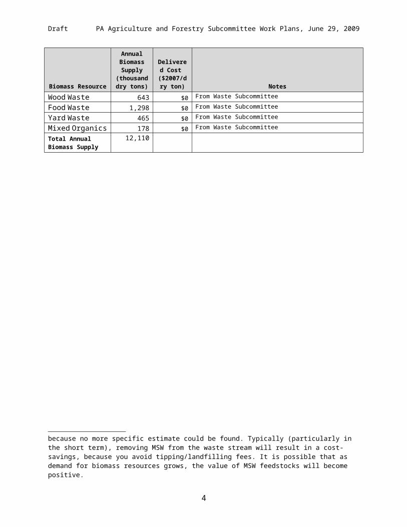
Table 1. Potential Annual Biomass Resource Supply in PA

Biomass Resource

AnnualBiomass Supply

(thousand dry tons)

Delivered Cost1

($2007/dry ton) Notes

Crop Residues 810$742 Biomass supply based on 2005 NREL Report.3

Potential Energy Crops (Switchgrass) 672

$854 2005 NREL Report.

Potential Energy Crops (Dry Poplar) 556

$855 2005 NREL Report.

Low-Use Wood 6000$586

http://www.dcnr.state.pa.us/PA_Biomass_guidance_final.pdf Based on estimate from Penn State's Dr. Charles Ray, 480 mm tons LUW x 2½ % growth = 12 million tons/yr * 50% for green/dry conversion = 6 mm dry tons/yr. 6 million tons of Low-Use Wood could be harvested in Pennsylvania annually. The Pennsylvania Department of Conservation and Natural Resources felt that this was overly optimistic, but did not provide a lower estimate.

Paper 1,488$0 From Waste Subcommittee7

Wood Waste 643 $0 From Waste Subcommittee

Food Waste 1,298 $0 From Waste Subcommittee

Yard Waste 465 $0 From Waste Subcommittee

Mixed Organics 178 $0 From Waste Subcommittee

Total Annual Biomass Supply

12,110

1 Delivered cost expressed in units of $/dry ton. 2 “Estimating a Value for Corn Stover” Ag Decision maker File A1-70, December 2007, http://www.extension.iastate.edu/agdm/crops/html/a1-70.html. The max a livestock owner would pay for corn stover as feed. Additional Transportation costs of $14.75 were assumed, taken from Iowa State University, University Extension, publication “Estimated Costs for Production, Storage and Transportation of Switchgrass”3 A. Milbrandt. A Geographic Perspective on the Current Biomass Resource Availability in the United States. Technical Report NREL/TP-560-39181. Golden, CO: U.S. Department of Energy, National Renewable Energy Laboratory, December 2005. Available at: www.nrel.gov/docs/fy06osti/39181.pdf.4 “Estimating the Economic Impact of Substituting Switchgrass for Coal for Electric Generation in Iowa.” Center for Global and Regional Environmental Research. University of Iowa. 2005. http://www.iowaswitchgrass.com/__docs/pdf/8-6-0%20Final%20Report.pdf5 Ibid. Same cost for Dry Poplar assumed as for switchgrass. 6 Based on information from John Karkash. Cited Woody biomass value at 29$/green ton. Converted to dry tons, results in a cost of $58/ton.7 Waste subcommittee provides estimates of MSW feedstocks. These estimates may change as recycling forecasts are modified. $0 cost for MSW feedstocks is used because no more specific estimate could be found. Typically (particularly in the short term), removing MSW from the waste stream will result in a cost-savings, because you avoid tipping/landfilling fees. It is possible that as demand for biomass resources grows, the value of MSW feedstocks will become positive.

2

http://www.nrel.gov/docs/fy06osti/39181.pdf


Agriculture-1. Foodshed Development Strategy

Strategy Name: Foodshed Development Strategy

Submitted by: Pennsylvania Association for Sustainable Agriculture

Lead Staff Contact: Brian Snyder, Executive Director

Parties Affected/Implementing Parties: Pennsylvania Departments of Environmental Protection (DEP), Agriculture (PDA), Conservation and Natural Resources (DCNR), Health (PDH), Community and Economic Development (DCED); Pennsylvania State Association of Township Supervisors (PSATS), county commissioners, school districts, colleges and universities, municipalities.

Goals: Foodshed analysis, Formation of foodshed policy teams, Development of strategic plans, Fund development, Granting and implementation, Creation of market-based, local investment opportunities

Initiative Summary:

This initiative would start with an economic, demographic, and land-use analysis of all of Pennsylvania to determine a limited number of “foodsheds,” where the utilization of locally produced and processed foods would be maximized and the use of fossil fuels in the procurement and delivery of the food would be minimized. To quantify greenhouse gas (GHG) reductions due to the use of local food, more data are needed on what food is being imported from where into the various regions of Pennsylvania. Packaged and processed foods are especially difficult to define, as they may use ingredients or elements from different states or countries.

After analysis of food origination is complete, the next implementation steps would include:

Granting authority to specialized “food policy teams” in each foodshed to work in conjunction with county governments to develop and implement “foodshed strategic plans” within a specified time.

Providing funds from the state and other sources in the form of grants to farmers, market venues, and municipalities wishing to participate. In addition, each team could maintain its own development function to raise funds through local foundations, businesses, and individuals to supplement state funds.

Establishing of backyard gardens (e.g., victory gardens), urban farming initiatives, farmers’ markets, community-supported agriculture (CSA) projects, cooperatives and on-farm or community-based processing facilities (e.g., meatpacking, creameries, packaging and storage of fruits and vegetables, etc.), and plans for consolidating transportation and distribution.

3


Data Sources/Assumptions/Methods for GHG: See relevant attachments.

Data Sources/Assumptions/Methods for Costs: Initial costs would be for foodshed analysis and strategic planning.

Potential Overlap: Not applicable.

Other: Here are links to the relevant Foodshed literature:

http://www.ruralpa.org/farm_school_report08.pdf

http://www.ruralpa.org/Farm_School_Guide08.pdf

http://www.farmandfoodproject.org/documents/uploads/The%20Case%20for%20Local%20&%20Regional%20Food%20Marketing.pdf

http://www.leopold.iastate.edu/research/marketing_files/NEIowa_042108.pdf

http://www.leopold.iastate.edu/pubs/staff/health/health.htm

http://www.leopold.iastate.edu/research/marketing_files/consumer_PNMWG5-05.pdf

http://www.leopold.iastate.edu/research/marketing_files/WorldBook.pdf

http://attra.ncat.org/attra-pub/PDF/foodmiles.pdf

http://www.leopold.iastate.edu/news/newsreleases/2007/organic_041807.htm

http://www.leopold.iastate.edu/pubs/staff/ppp/index.htm

http://www.leopold.iastate.edu/research/marketing_files/GoodFoodIowa_0408.pdf

4

http://www.leopold.iastate.edu/research/marketing_files/GoodFoodIowa_0408.pdf

http://www.leopold.iastate.edu/pubs/staff/ppp/index.htm

http://www.leopold.iastate.edu/news/newsreleases/2007/organic_041807.htm

http://attra.ncat.org/attra-pub/PDF/foodmiles.pdf

http://www.leopold.iastate.edu/research/marketing_files/WorldBook.pdf

http://www.leopold.iastate.edu/research/marketing_files/consumer_PNMWG5-05.pdf

http://www.leopold.iastate.edu/pubs/staff/health/health.htm

http://www.leopold.iastate.edu/research/marketing_files/NEIowa_042108.pdf



http://www.ruralpa.org/Farm_School_Guide08.pdf

http://www.ruralpa.org/farm_school_report08.pdf


Agriculture-2. Next-Generation Biofuels

Submitted by: Commonwealth of Pennsylvania and Chesapeake Bay Commission

Lead Staff Contact: Marel Raub, Pennsylvania Director, Chesapeake Bay Commission, 717-772-3651Lindsey Harteis, 717-783-6986

Parties Affected/Implementing Parties: DEP, U.S. Environmental Protection Agency (EPA) Chesapeake Bay Program Office, feedstock producers, biofuel producers.

Goals: Provide sufficient biofuels to fulfill Pennsylvania’s share of the federal Renewable Fuels Standard (RFS). This means that 545 million gallons (MMgal) of biofuel will need to be produced in Pennsylvania in 2020.

Implementation Period: Increase production such that by 2020 Pennsylvania is producing 545 MMgal of biofuel.

Summary: This work plan quantified the amount of biofuel necessary to meet Pennsylvania's share of the federal RFS. It also considers the technical potential of biofuel production based on available feedstocks.

Implementation Steps: Commonwealth policy should encourage:

The production of feedstocks for biofuel, including winter crops. Biofuel producers to utilize these crops as a feedstock. The establishment of coordinated systems for biofuel production, including corn-

based and cellulosic ethanol and biodiesel fuels, with economic incentives to agricultural producers to ensure the sufficient commitment of production of corn, soybean, and plant materials for biofuel use.

Data Sources/Assumptions/Methods for GHG:

Biofuel RequiredThe GHG reductions for this option are dependent on developing in-state production capacity that achieves GHG reductions beyond petroleum fuels. This option quantifies the GHG reductions and costs of producing sufficient renewable liquid biofuels to meet Pennsylvania’s share (3.63%) of the federal RFS. The three biofuels being considered in this analysis are cellulosic ethanol, soy/grease biodiesel, and algae biodiesel.

Corn ethanol was not considered because it provides lower GHG reductions compared to other biofuels. Pennsylvania produced 23 MMgal of soy/grease biodiesel in 2008, and this production is projected to increase through 2013.8 For 2014–2020, all growth in biodiesel production is

8 Based on personal communication with Mike Rader by Jackson Schreiber. 5/6/09.

5


assumed to take the form of algae biodiesel, which is less land intensive and provides greater GHG reductions than first-generation biofuels.

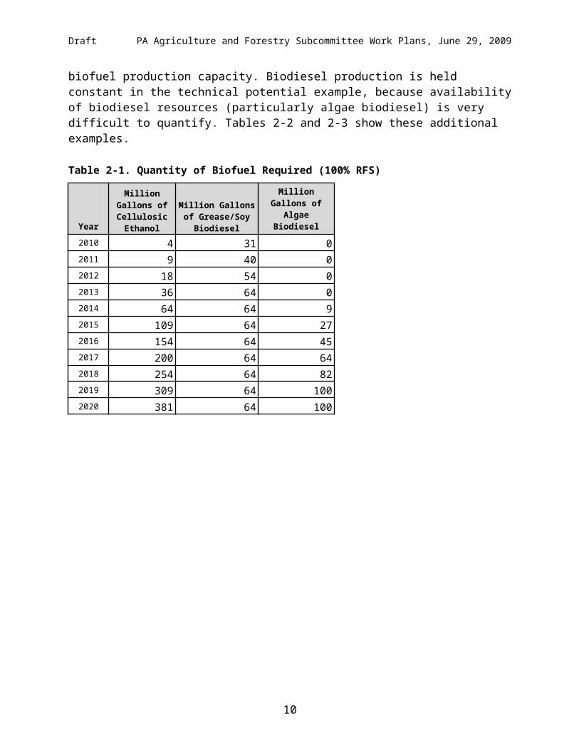
Table 2-1 outlines the amounts of each type of fuel that will be needed to fulfill Pennsylvania’s share of the RFS. This is the amount of biofuel that is assumed to be produced in the analysis, and will be given to the Transportation and Land Use (TLU) and Residential, Commercial, and Industrial (RCI) (for heating-oil biodiesel use) Technical Work Groups (TWGs) as available in-state biofuel.

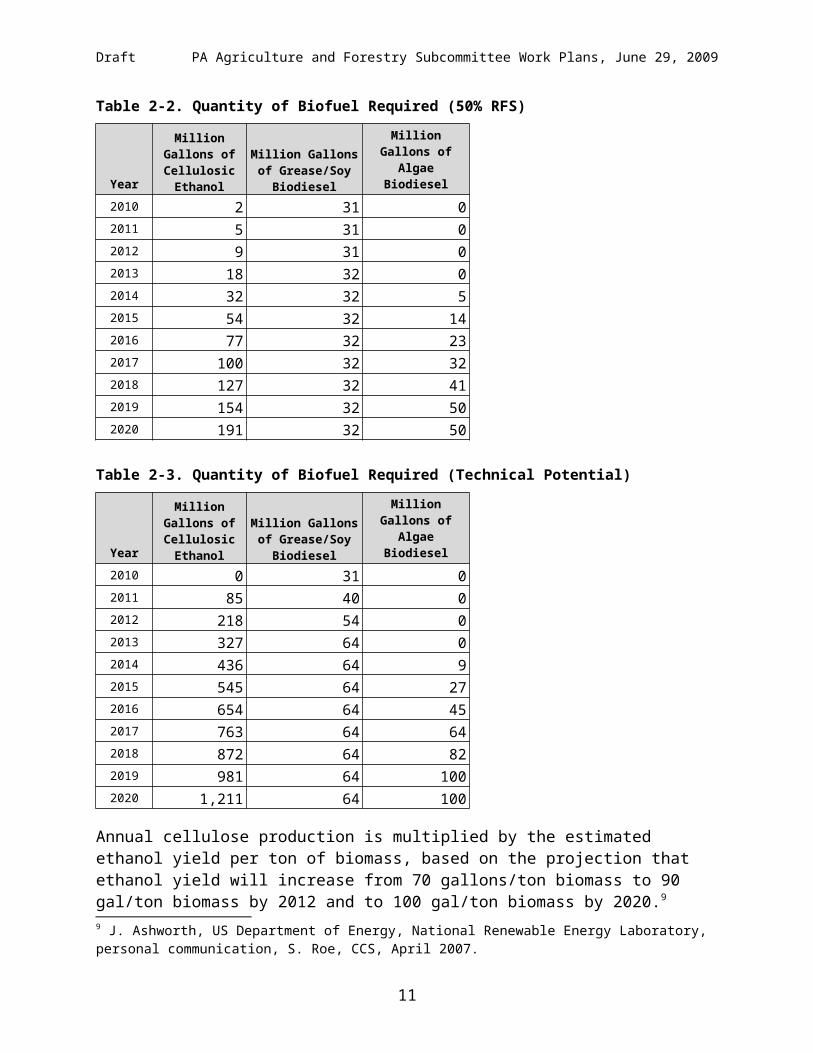
To illustrate the costs and GHG reductions of different levels of production, this analysis will also consider the costs of producing one-half Pennsylvania’s share of the RFS and also maximum technical potential available if all available biomass resources were going toward cellulosic biofuel production. To get this third estimate, it must be assumed that there are no other demands upon biomass resources in the state in 2020 (which is very unlikely), and that a huge effort has been made to expand biofuel production capacity. Biodiesel production is held constant in the technical potential example, because availability of biodiesel resources (particularly algae biodiesel) is very difficult to quantify. Tables 2-2 and 2-3 show these additional examples.

Table 2-1. Quantity of Biofuel Required (100% RFS)

Year

Million Gallons of Cellulosic

Ethanol

Million Gallons of Grease/Soy Biodiesel

Million Gallons of Algae Biodiesel

2010 4 31 02011 9 40 02012 18 54 02013 36 64 02014 64 64 92015 109 64 272016 154 64 452017 200 64 642018 254 64 822019 309 64 1002020 381 64 100

6


Table 2-2. Quantity of Biofuel Required (50% RFS)

Year


Ethanol



2010 2 31 02011 5 31 02012 9 31 02013 18 32 02014 32 32 52015 54 32 142016 77 32 232017 100 32 322018 127 32 412019 154 32 502020 191 32 50

Table 2-3. Quantity of Biofuel Required (Technical Potential)

Year


Ethanol



2010 0 31 02011 85 40 02012 218 54 02013 327 64 02014 436 64 92015 545 64 272016 654 64 452017 763 64 642018 872 64 822019 981 64 1002020 1,211 64 100

Annual cellulose production is multiplied by the estimated ethanol yield per ton of biomass, based on the projection that ethanol yield will increase from 70 gallons/ton biomass to 90 gal/ton biomass by 2012 and to 100 gal/ton biomass by 2020.9 Table 2-4 shows the number of 70-MMgal/year cellulosic plants that will need to go on line in Pennsylvania to provide the biofuel needed to meet Pennsylvania’s share of the RFS. Table 2-5 shows the number of plants needed for 50% of the RFS, and Table 2-6 shows the number of plants needed if all technically available biomass is going toward cellulosic ethanol production in 2020. All plants are not expressed in whole numbers, and in such a case should be assumed to be operating at less than full capacity during the given year.

9 J. Ashworth, US Department of Energy, National Renewable Energy Laboratory, personal communication, S. Roe, CCS, April 2007.

7


Table 2-4. Projected Biofuel Production (100% RFS)

Year

EtOH yield from cellulosic feedstock (gal/ton biomass)*

Cellulosic Ethanol

Production Plants

Required

Cellulosic Ethanol Required to meet goal (million gallons)

Biomass Required (million dry tons)

2010 70 0.1 4 0.1 2011 70 0.1 9 0.1 2012 90 0.3 18 0.2 2013 90 0.5 36 0.4 2014 90 0.9 64 0.7 2015 90 1.6 109 1.2 2016 90 2.2 154 1.7 2017 90 2.9 200 2.2 2018 90 3.7 254 2.8 2019 90 4.5 309 3.4 2020 100 5.5 381 3.8

* source: J. Ashworth, NREL, personal communication, 4/06/07.Note: Cellulosic plants required are not whole numbers. The analysis assumes that these plants will be going on line mid-year or operating at less than full capacity.

Table 2-5. Projected Biofuel Production (50% RFS)

Year


Cellulosic Ethanol Production Plants Required



2010 70 0.0 2 0.0 2011 70 0.1 5 0.1 2012 90 0.1 9 0.1 2013 90 0.3 18 0.2 2014 90 0.5 32 0.4 2015 90 0.8 54 0.6 2016 90 1.1 77 0.9 2017 90 1.4 100 1.1 2018 90 1.8 127 1.4 2019 90 2.2 154 1.7 2020 100 2.8 191 1.9


8


Table 2-6. Projected Biofuel Production (Technical Potential)

Year


Cellulosic Ethanol Production Plants Required



2010 70 0.0 0 0.0 2011 70 1.2 85 1.2 2012 90 3.1 218 2.4 2013 90 4.7 327 3.6 2014 90 6.3 436 4.8 2015 90 7.9 545 6.1 2016 90 9.4 654 7.3 2017 90 11.0 763 8.5 2018 90 12.6 872 9.7 2019 90 14.2 981 10.9 2020 100 17.5 1,211 12.1


The GHG savings of biofuel production and consumption are accounted for in the TLU analysis (T-2). This analysis instead focuses on the total costs of biofuel production, the amount of biofuels required, and the wholesale $/gal for each biofuel produced.

Biofuel Costs

Cellulosic Ethanol CostsThe cellulosic ethanol costs of this option are estimated based on the capital and operating costs of cellulosic ethanol production plants. A study by the National Renewable Energy Laboratory (NREL) was used to estimate the operation and maintenance (O&M) costs of a 70-MMgal/yr cellulosic ethanol plant.10 The capital costs of a cellulosic plant came from an average of the capital cost estimates for six biofuels plants across the country. Using this method, the average capital cost of a new cellulosic ethanol plant is $549 million. A new plant will need to be built for every 70 MMgal of annual ethanol production needed. It was assumed that the capital costs will be paid according to a cost recovery factor over the 20-year lifetime of the plant. The cost of biomass feedstocks made up a significant portion (~60%) of variable costs. Therefore, we replaced the NREL estimate of feedstock costs ($30/ton) with more current estimates of the cost

10 National Renewable Energy Laboratory, Lignocellulosic Biomass to Ethanol Process Design and Economics Utilizing Co-Current Dilute Acid Prehydrolysis and Enzymatic Hydrolysis for Corn Stover, NREL/ TP-510-32438 (Golden, CO, June 2002), www. nrel.gov/docs/fy02osti/32438.pdf, accessed June 2008.

9


of delivered biomass: $74/ton for agricultural feedstocks11 and $58/ton for woody feedstocks.12 Energy crops were estimated to cost $85/ton.13

Municipal solid waste (MSW) costs are very difficult to estimate. Most MSW landfills charge a tipping fee. Therefore, there is a cost savings when waste is delivered to a cellulosic facility, rather than a landfill. However, in the interest of providing a more conservative estimate, a $0/ton estimate was used for MSW costs.

Other annual costs cover unavoidable expenses of running an ethanol plant, such as employee wages, insurance, maintenance, etc. The plant proposed by the NREL study produces some excess electricity, although the costs and GHG reductions of generating this electricity are not considered in this analysis.

Which feedstocks will be used in cellulosic ethanol is difficult to determine. It was assumed that a mix of all feedstocks would be used, based on a percentage of each with respect to overall availability (which can be seen on page 2 of this analysis).

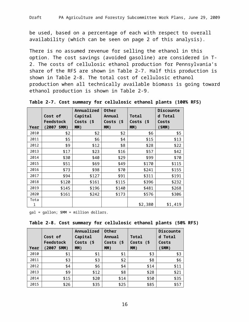
There is no assumed revenue for selling the ethanol in this option. The cost savings (avoided gasoline) are considered in T-2. The costs of cellulosic ethanol production for Pennsylvania’s share of the RFS are shown in Table 2-7. Half this production is shown in Table 2-8. The total cost of cellulosic ethanol production when all technically available biomass is going toward ethanol production is shown in Table 2-9.

Table 2-7. Cost summary for cellulosic ethanol plants (100% RFS)

Year

Cost of Feedstock (2007 $MM)

Annualized Capital Costs ($ MM)

Other Annual Costs ($ MM)

Total Costs ($ MM)

Discounted Total Costs ($MM)

2010 $2 $2 $2 $6 $52011 $5 $6 $4 $15 $132012 $9 $12 $8 $28 $222013 $17 $23 $16 $57 $422014 $30 $40 $29 $99 $702015 $51 $69 $49 $170 $1152016 $73 $98 $70 $241 $1552017 $94 $127 $91 $311 $1912018 $120 $161 $115 $396 $2322019 $145 $196 $140 $481 $268

11 “Estimating a Value for Corn Stover” Ag Decision maker File A1-70, December 2007, http://www.extension.iastate.edu/agdm/crops/html/a1-70.html. The max a livestock owner would pay for corn stover as feed. Additional Transportation costs of $14.75 were assumed, taken from Iowa State University, University Extension, publication “Estimated Costs for Production, Storage and Transportation of Switchgrass”12 Based on information from John Karkash. Cited Woody biomass value at 29$/green ton. Converted to dry tons, results in a cost of $58/ton.13 “Estimating the Economic Impact of Substituting Switchgrass for Coal for Electric Generation in Iowa.” Center for Global and Regional Environmental Research. University of Iowa. 2005. http://www.iowaswitchgrass.com/__docs/pdf/8-6-0%20Final%20Report.pdf

10


Year




Total Costs ($ MM)


2020 $161 $242 $173 $576 $306Total $2,380 $1,419

gal = gallon; $MM = million dollars.

Table 2-8. Cost summary for cellulosic ethanol plants (50% RFS)

Year




Total Costs ($ MM)


2010 $1 $1 $1 $3 $32011 $3 $3 $2 $8 $62012 $4 $6 $4 $14 $112013 $9 $12 $8 $28 $212014 $15 $20 $14 $50 $352015 $26 $35 $25 $85 $572016 $36 $49 $35 $120 $782017 $47 $63 $45 $156 $962018 $60 $81 $58 $198 $1162019 $73 $98 $70 $241 $1342020 $81 $121 $86 $288 $153Total $1,190 $709


Table 2-9. Cost summary for cellulosic ethanol plants (Technical Potential)

Year




Total Costs ($ MM)


2010 $0 $0 $0 $0 $02011 $51 $54 $38 $143 $1182012 $102 $138 $99 $340 $2662013 $154 $207 $148 $509 $3802014 $205 $277 $198 $679 $4832015 $256 $346 $247 $849 $5742016 $307 $415 $296 $1,019 $6572017 $359 $484 $346 $1,188 $7302018 $410 $553 $395 $1,358 $7942019 $461 $622 $444 $1,528 $8512020 $512 $768 $549 $1,829 $970Total $9,442 $5,822

11



Soy/Waste Grease Biodiesel Costs

Biodiesel from soy and waste grease was the only biofuel produced in Pennsylvania in 2008. This production is expected to increase until 2013, at which point production of these first-generation biofuels will remain constant, and algae biodiesel production will begin increasing. The costs of biodiesel production from waste grease and soy come from the U.S. Energy Information Administration (EIA), which predicted the wholesale price of both fuels through 201214 (EIA, 2004). These estimates are then held constant through 2020.

The costs of this option are also dependent on the ratio of waste grease and soy in the biodiesel. Because waste grease is more cost-effective, these supplies will be used first. However, it is unlikely that grease supplies can be expanded significantly from their current levels. It is assumed that waste grease supplies remain relatively constant (capable of producing 17 MMgal/yr), and all additional biodiesel production must come from soy oil. It is possible that other feedstocks will be used for biodiesel production, such as semolina, but soy is used as an example of feedstock costs in this analysis. This is used to estimate the overall production costs of biodiesel in Pennsylvania through 2020.

The TLU analysis requires that we provide costs for each biofuel. These costs are based on the production costs, although there are other costs that must be accounted for in order to estimate the cost at the pump. It can be difficult to estimate the difference in fuel costs between wholesale (cost to the producer) and retail (cost to the consumer). The EIA Annual Energy Outlook 2008 (AEO 2008) does not estimate wholesale costs of biodiesel, but does estimate wholesale costs of corn ethanol. When these costs are compared to the retail cost estimates, the markup is 45–65 cents/gal.15 This figure is used as a stand-in for the cost difference between wholesale and retail biodiesel. The costs of producing Pennsylvania’s share of the federal RFS are shown in Table 2-10. Table 2-11 shows half of that amount. The maximum technical feasibility of biodiesel feedstocks is not easy to calculate in this analysis; therefore, the technically feasible amount is assumed to match that of Table 2-10 for biodiesel production.

14 US EIA. Radich, Anthony. “Biodiesel Performance, Costs, and Use”. 2004. http://www.eia.doe.gov/oiaf/analysispaper/biodiesel/

15 US EIA. Annual Energy Outlook 2008. http://www.eia.doe.gov/oiaf/archive/aeo08/index.html

12

http://www.eia.doe.gov/oiaf/archive/aeo08/index.html

http://www.eia.doe.gov/oiaf/analysispaper/biodiesel/


Table 2-10. Soy/Waste Grease Production Costs (100% RFS)

Year

Gen 1 Biodiesel Displacement Goal (Million

Gals)

Wholesale Waste Grease

Cost ($/gal)

Wholesale Soy

Biodiesel Cost ($/Gal)

Wholesale Cost Gen 1 Biodiesel

($/Gal)

Retail Cost, Gen 1

Biodiesel ($/Gal)

Production Costs of

Gen 1 Biodiesel

($MM)2010 31 $1.88 $3.41 $2.55 $3.00 $93 2011 40 $1.93 $3.48 $2.81 $3.35 $134 2012 54 $1.98 $3.57 $3.06 $3.67 $200 2013 64 $1.98 $3.57 $3.13 $3.73 $237 2014 64 $1.98 $3.57 $3.13 $3.67 $233 2015 64 $1.98 $3.57 $3.13 $3.50 $223 2016 64 $1.98 $3.57 $3.13 $3.76 $239 2017 64 $1.98 $3.57 $3.13 $3.83 $244 2018 64 $1.98 $3.57 $3.12 $3.79 $241 2019 64 $1.98 $3.57 $3.12 $3.77 $239 2020 64 $1.98 $3.57 $3.12 $3.75 $239 Total $2,321

Table 2-11. Soy/Waste Grease Production Costs (50% RFS)

Year

Gen 1 Biodiesel Displacement Goal (Million

Gals)

Wholesale Waste Grease

Cost ($/gal)

Wholesale Soy

Biodiesel Cost ($/Gal)

Wholesale Cost Gen 1 Biodiesel

($/Gal)

Retail Cost, Gen 1

Biodiesel ($/Gal)

Production Costs of

Gen 1 Biodiesel

($MM)2010 31 $1.88 $3.41 $2.55 $3.00 $932011 31 $1.93 $3.48 $2.61 $3.16 $972012 31 $1.98 $3.57 $2.67 $3.28 $1012013 32 $1.98 $3.57 $2.70 $3.29 $1052014 32 $1.98 $3.57 $2.69 $3.23 $1032015 32 $1.98 $3.57 $2.69 $3.06 $972016 32 $1.98 $3.57 $2.68 $3.31 $1052017 32 $1.98 $3.57 $2.68 $3.39 $1082018 32 $1.98 $3.57 $2.67 $3.34 $1062019 32 $1.98 $3.57 $2.67 $3.32 $1052020 32 $1.98 $3.57 $2.67 $3.30 $105Total $1,125

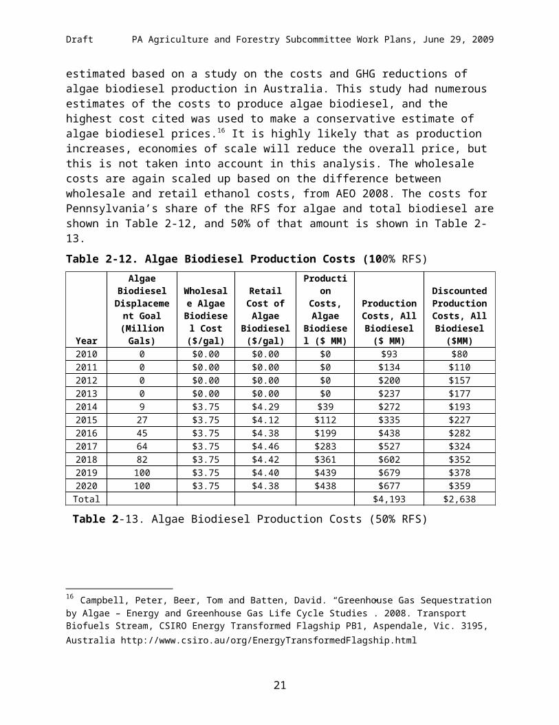
Algae Biodiesel CostsKeystone Biofuels is working on pre-commercial biodiesel production in Pennsylvania, and commercial algae biodiesel production is assumed to begin by 2014. Algae biodiesel costs are estimated based on a study on the costs and GHG reductions of algae biodiesel production in Australia. This study had numerous estimates of the costs to produce algae biodiesel, and the highest cost cited was used to make a conservative estimate of algae biodiesel prices.16 It is

16 Campbell, Peter, Beer, Tom and Batten, David. “Greenhouse Gas Sequestration by Algae – Energy and Greenhouse Gas Life Cycle Studies”. 2008. Transport Biofuels Stream, CSIRO Energy Transformed Flagship PB1,

13


highly likely that as production increases, economies of scale will reduce the overall price, but this is not taken into account in this analysis. The wholesale costs are again scaled up based on the difference between wholesale and retail ethanol costs, from AEO 2008. The costs for Pennsylvania’s share of the RFS for algae and total biodiesel are shown in Table 2-12, and 50% of that amount is shown in Table 2-13.

Table 2-12. Algae Biodiesel Production Costs (100% RFS)

Year

Algae Biodiesel

Displacement Goal (Million

Gals)

Wholesale Algae

Biodiesel Cost

($/gal)

Retail Cost of Algae Biodiesel

($/gal)

Production Costs, Algae

Biodiesel ($ MM)

Production Costs, All

Biodiesel ($ MM)

Discounted Production Costs, All Biodiesel

($MM)2010 0 $0.00 $0.00 $0 $93 $802011 0 $0.00 $0.00 $0 $134 $1102012 0 $0.00 $0.00 $0 $200 $1572013 0 $0.00 $0.00 $0 $237 $1772014 9 $3.75 $4.29 $39 $272 $1932015 27 $3.75 $4.12 $112 $335 $2272016 45 $3.75 $4.38 $199 $438 $2822017 64 $3.75 $4.46 $283 $527 $3242018 82 $3.75 $4.42 $361 $602 $3522019 100 $3.75 $4.40 $439 $679 $3782020 100 $3.75 $4.38 $438 $677 $359Total $4,193 $2,638

Table 2-13. Algae Biodiesel Production Costs (50% RFS)

Year

Algae Biodiesel

Displacement Goal (Million

Gals)

Wholesale Algae

Biodiesel Cost

($/gal)


($/gal)

Production Costs, Algae

Biodiesel ($ MM)

Production Costs, All

Biodiesel ($ MM)


($MM)2010 0 $0.00 $0.00 $0 $93 $802011 0 $0.00 $0.00 $0 $97 $802012 0 $0.00 $0.00 $0 $101 $792013 0 $0.00 $0.00 $0 $105 $782014 5 $3.75 $4.29 $19 $122 $872015 14 $3.75 $4.12 $56 $153 $1042016 23 $3.75 $4.38 $99 $205 $1322017 32 $3.75 $4.46 $142 $249 $1532018 41 $3.75 $4.42 $181 $287 $1682019 50 $3.75 $4.40 $220 $325 $1812020 50 $3.75 $4.38 $219 $324 $172Total $2,061 $1,313

Total biofuel costs are shown in Table 2-14 for 100% of PA’s share of the RFS, Table 2-15 for 50% of PA’s share, and Table 2-16 for the technical potential. The costs shown in these tables are discounted back to 2007 dollars, using a 5% discount rate.

Table 2-14. Total biofuel costs (100%RFS)

Aspendale, Vic. 3195, Australia http://www.csiro.au/org/EnergyTransformedFlagship.html

14


Year

Discounted Cellulosic

Costs ($MM)


($MM)

Discounted Biofuel Costs

($MM)2010 $5 $80 $852011 $13 $110 $1232012 $22 $157 $1792013 $42 $177 $2192014 $70 $193 $2642015 $115 $227 $3422016 $155 $282 $4372017 $191 $324 $5152018 $232 $352 $5842019 $268 $378 $6462020 $306 $359 $664Total $4,057

$MM = millions of dollars.

Table 2-15. Total biofuel costs (50%RFS)

Year


Costs ($MM)


($MM)


($MM)2010 $3 $80 $832011 $6 $80 $872012 $11 $79 $902013 $21 $78 $992014 $35 $87 $1222015 $57 $104 $1612016 $78 $132 $2092017 $96 $153 $2492018 $116 $168 $2832019 $134 $181 $3152020 $153 $172 $325Total $2,023


Table 2-16. Total biofuel costs (Technical Potential)

Year


Costs ($MM)


($MM)


($MM)

15


2010 $0 $80 $802011 $118 $110 $2282012 $266 $157 $4232013 $380 $177 $5572014 $483 $193 $6762015 $574 $227 $8012016 $657 $282 $9392017 $730 $324 $1,0532018 $794 $352 $1,1462019 $851 $378 $1,2292020 $970 $359 $1,329Total $8,461


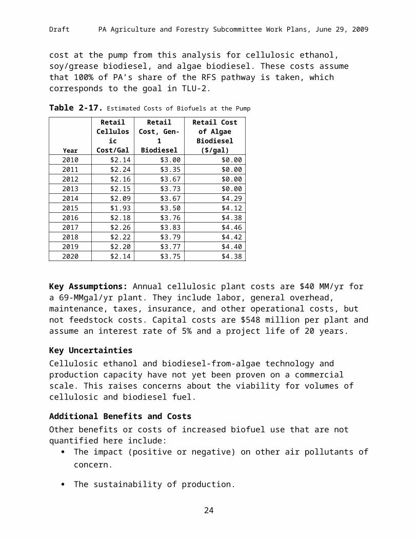
The costs of delivered biomass are be used for the cost-effectiveness analysis in TLU-2. Table 2-17 shows the estimated cost at the pump from this analysis for cellulosic ethanol, soy/grease biodiesel, and algae biodiesel. These costs assume that 100% of PA’s share of the RFS pathway is taken, which corresponds to the goal in TLU-2.

Table 2-17. Estimated Costs of Biofuels at the Pump

Year

Retail Cellulosic Cost/Gal

Retail Cost, Gen-1

Biodiesel


($/gal)2010 $2.14 $3.00 $0.002011 $2.24 $3.35 $0.002012 $2.16 $3.67 $0.002013 $2.15 $3.73 $0.002014 $2.09 $3.67 $4.292015 $1.93 $3.50 $4.122016 $2.18 $3.76 $4.382017 $2.26 $3.83 $4.462018 $2.22 $3.79 $4.422019 $2.20 $3.77 $4.402020 $2.14 $3.75 $4.38

Key Assumptions: Annual cellulosic plant costs are $40 MM/yr for a 69-MMgal/yr plant. They include labor, general overhead, maintenance, taxes, insurance, and other operational costs, but not feedstock costs. Capital costs are $548 million per plant and assume an interest rate of 5% and a project life of 20 years.

Key UncertaintiesCellulosic ethanol and biodiesel-from-algae technology and production capacity have not yet been proven on a commercial scale. This raises concerns about the viability for volumes of cellulosic and biodiesel fuel.

16


Additional Benefits and CostsOther benefits or costs of increased biofuel use that are not quantified here include:

The impact (positive or negative) on other air pollutants of concern.

The sustainability of production.

Flexibility to adjust based on the emergence of other technologies that might result in greater or more cost-effective GHG reductions.

The impact on food prices.

The impact on fuel tax revenue.

The impact on the cost of delivering goods (i.e., fuel prices).

Other environmental impacts, such as water quality and quantity, and conservation of land. Winter crops provide significant water quality benefits by removing excess nitrogen from the soil. From analyses of Pennsylvania cropping systems for the purpose of water quality improvements, there is significant acreage in the state that is available to produce winter crops that is not already used for this purpose.

Secondary land-use impacts.

Security benefits from domestic fuel production.

References:

Potential contacts for information include:Mark DubinAgricultural Technical CoordinatorChesapeake Bay Program Office410-267-9833 TEL

Dr. Tom Richard, DirectorPenn State Institutes of Energy and the Environment(814) 865-3722

Potential Overlap: This work plan has overlap with the Residential work plan B5 Biofuel Incentives, where biodiesel will be used as an additive in home heating oil and with the Transportation-2 Biofuels work plan.

Other Considerations: For both GHG and water quality reasons, a transition to a regional biofuels industry based on cellulosic and other next-generation feedstocks is desirable. However, this transition will not be instantaneous, and anything that can be done in the interim to facilitate that transition will be advantageous.

17


Much has been made of the “chicken-and-egg” problem facing new biofuel production endeavors. Feedstock producers are reluctant to invest in new crops and cropping systems without a sure market, and biofuel producers are reluctant to rely on a feedstock without a clear supply. To minimize this dilemma when cellulosic ethanol technologies ultimately become commercially feasible, action must be taken now to create a growing supply of cellulosic material that also meets current needs.

Winter crops, such as barley, can serve this purpose. The grain can be used as a feedstock for first-generation ethanol technology as a substitute for corn. The straw can support existing biomass combustion efforts and can be used as a cellulosic feedstock when that technology becomes available. In the meantime, the current technologies drive increased plantings of the winter crops, resulting in a relatively predictable supply of cellulosic material down the road.

18


Agriculture-3. Management-Intensive Grazing

Submitted by: Pennsylvania Association for Sustainable Agriculture

Lead Staff Contact: Brian Snyder, Executive Director

Parties Affected/Implementing Parties: PDA, Natural Resources Conservation Service (NRCS), DEP, DCED, DCNR.

Goals: Double the number of acres under management-intensive grazing (MiG) by 2020.

Implementation Period: The implementation of this option will proceed with a linear increase in additional MiG acres between 2010 and 2020.

Initiative Summary: This initiative would create incentives and provide support for farmers wishing to transition their livestock operations from grain-intensive practices (which usually requiring the importing of grain/nutrients into the region) to continuous MiG, which by contrast takes advantage of more local resources and increases sequestered carbon in pasturelands.

In addition to the implementation of MiG on farms, the initiative would help in marketing Pennsylvania-grown, pasture-based products to Pennsylvanians. A strategy of “Eating the View” would emphasize the need for consumers to choose products that help to maintain the bucolic pasturelands for which Pennsylvania is famous, while also improving their own nutrition and the health of the planet by sequestering more carbon through intensive grass production.

Implementation Steps: Provide incentives for farmers/grazers/ranchers to transition to MiG.

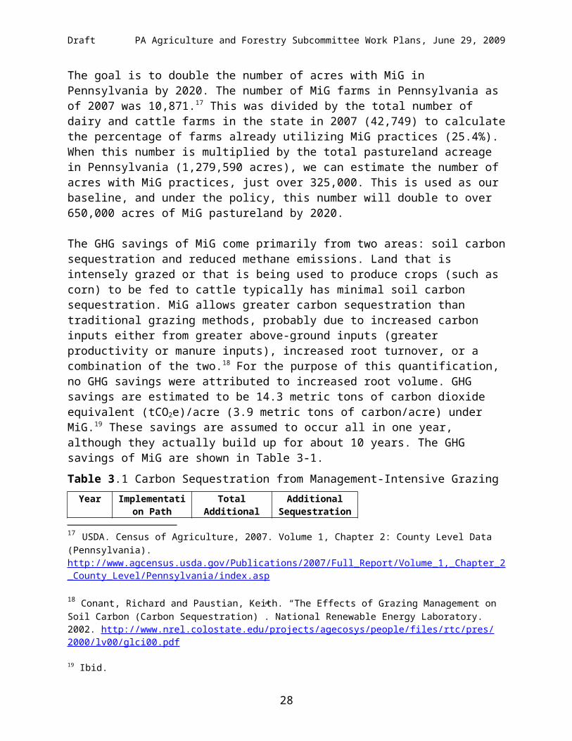
Estimated GHG Reductions and Net Costs or Cost SavingsGHG Reductions from MiGThe goal is to double the number of acres with MiG in Pennsylvania by 2020. The number of MiG farms in Pennsylvania as of 2007 was 10,871.17 This was divided by the total number of dairy and cattle farms in the state in 2007 (42,749) to calculate the percentage of farms already utilizing MiG practices (25.4%). When this number is multiplied by the total pastureland acreage in Pennsylvania (1,279,590 acres), we can estimate the number of acres with MiG practices, just over 325,000. This is used as our baseline, and under the policy, this number will double to over 650,000 acres of MiG pastureland by 2020.

The GHG savings of MiG come primarily from two areas: soil carbon sequestration and reduced methane emissions. Land that is intensely grazed or that is being used to produce crops (such as corn) to be fed to cattle typically has minimal soil carbon sequestration. MiG allows greater carbon sequestration than traditional grazing methods, probably due to increased carbon inputs either from greater above-ground inputs (greater productivity or manure inputs), increased root

17 USDA. Census of Agriculture, 2007. Volume 1, Chapter 2: County Level Data (Pennsylvania). http://www.agcensus.usda.gov/Publications/2007/Full_Report/Volume_1,_Chapter_2_County_Level/Pennsylvania/index.asp

19

http://www.agcensus.usda.gov/Publications/2007/Full_Report/Volume_1,_Chapter_2_County_Level/Pennsylvania/index.asp



turnover, or a combination of the two.18 For the purpose of this quantification, no GHG savings were attributed to increased root volume. GHG savings are estimated to be 14.3 metric tons of carbon dioxide equivalent (tCO2e)/acre (3.9 metric tons of carbon/acre) under MiG.19 These savings are assumed to occur all in one year, although they actually build up for about 10 years. The GHG savings of MiG are shown in Table 3-1.

Table 3.1 Carbon Sequestration from Management-Intensive Grazing

YearImplementation

Path

Total Additional Acres of

Beef/Dairy Cattle

Additional Sequestration

(MMtCO2e)2010 0% 0 02011 10% 32,540 0.472012 20% 65,080 0.472013 30% 97,619 0.472014 40% 130,159 0.472015 50% 162,699 0.472016 60% 195,239 0.472017 70% 227,778 0.472018 80% 260,318 0.472019 90% 292,858 0.472020 100% 325,398 0.47Total 4.65

There are also GHG savings that result from reduced methane emissions. Cattle digest grass through a natural process called enteric fermentation. Enteric fermentation results in methane emissions, which can vary depending on the amount and type of feed given to the cattle. MiG practices reduce the overall amount of feed and generally result in a diet that is easier to digest than the diet given to cattle in confined feeding operations.20 While methane emission reductions can vary based on other factors, an average reduction of 22% was found when MiG practices were implemented.21 These are applied to all animals in this analysis, as shown in Table 3-2.

18 Conant, Richard and Paustian, Keith. “The Effects of Grazing Management on Soil Carbon (Carbon Sequestration)”. National Renewable Energy Laboratory. 2002. http://www.nrel.colostate.edu/projects/agecosys/people/files/rtc/pres/2000/lv00/glci00.pdf

19 Ibid.20 DeRamus, H.A. Clement, T.C., Giampola, D.D., and Dickinson, Peter. “Methane Emissions of Beef Cattle on Forages: Efficiency of Grazing Management Systems”. Journal of Environmental Quality. 2003. http://jeq.scijournals.org/cgi/reprint/32/1/269.pdf

21 DeRamus, H.A. Clement, T.C., Giampola, D.D., and Dickinson, Peter. “Methane Emissions of Beef Cattle on Forages: Efficiency of Grazing Management Systems”. Journal of Environmental Quality. 2003. http://jeq.scijournals.org/cgi/reprint/32/1/269.pdf

20

http://jeq.scijournals.org/cgi/reprint/32/1/269.pdf


http://www.nrel.colostate.edu/projects/agecosys/people/files/rtc/pres/2000/lv00/glci00.pdf


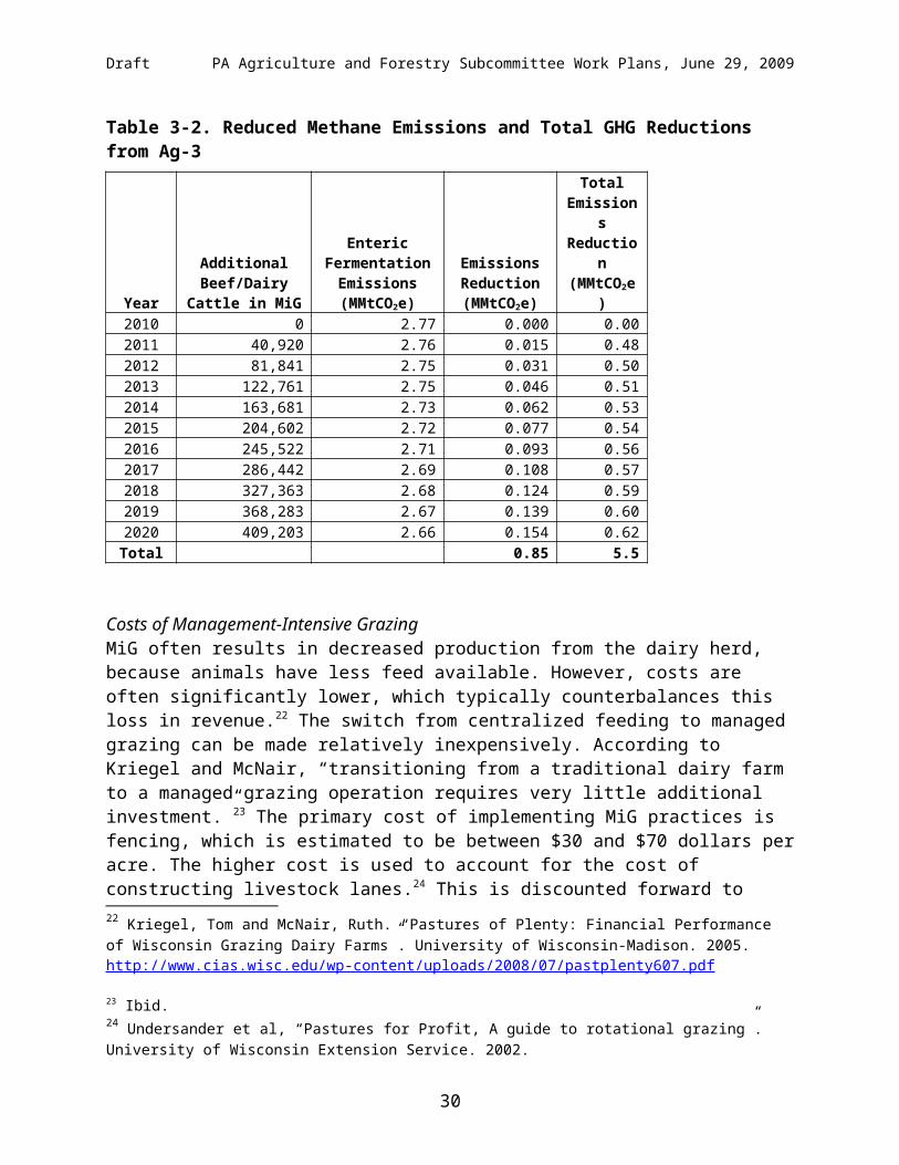
Table 3-2. Reduced Methane Emissions and Total GHG Reductions from Ag-3

Year

Additional Beef/Dairy Cattle

in MiG

Enteric Fermentation

Emissions (MMtCO2e)

Emissions Reduction (MMtCO2e)

Total Emissions Reduction (MMtCO2e)

2010 0 2.77 0.000 0.002011 40,920 2.76 0.015 0.482012 81,841 2.75 0.031 0.502013 122,761 2.75 0.046 0.512014 163,681 2.73 0.062 0.532015 204,602 2.72 0.077 0.542016 245,522 2.71 0.093 0.562017 286,442 2.69 0.108 0.572018 327,363 2.68 0.124 0.592019 368,283 2.67 0.139 0.602020 409,203 2.66 0.154 0.62Total 0.85 5.5

Costs of Management-Intensive GrazingMiG often results in decreased production from the dairy herd, because animals have less feed available. However, costs are often significantly lower, which typically counterbalances this loss in revenue.22 The switch from centralized feeding to managed grazing can be made relatively inexpensively. According to Kriegel and McNair, “transitioning from a traditional dairy farm to a managed grazing operation requires very little additional investment.”23 The primary cost of implementing MiG practices is fencing, which is estimated to be between $30 and $70 dollars per acre. The higher cost is used to account for the cost of constructing livestock lanes.24 This is discounted forward to reflect 2007 dollars, and applied to the first year MiG practices are implemented, as shown in Table 3-3.

There are also associated costs and cost savings that come from maintaining MiG practices. Costs come primarily in the form of reduced yield (beef sold or milk produced), and costs savings come from reduced inputs, such as corn to be fed to the cattle. A survey of profitability of different farm types over seven years found that net farm income for dairy operators was higher for managed grazing ($524/head) than for traditional confinement ($245/head) or large-scale confinement practices ($131/head).25 These costs are also shown in Table 3-3. Final costs are discounted back to 2007 dollars using a 5% discount rate. Additional information on the cost-

22 Kriegel, Tom and McNair, Ruth. “Pastures of Plenty: Financial Performance of Wisconsin Grazing Dairy Farms”. University of Wisconsin-Madison. 2005. http://www.cias.wisc.edu/wp-content/uploads/2008/07/pastplenty607.pdf

23 Ibid.24 Undersander et al, “Pastures for Profit, A guide to rotational grazing”. University of Wisconsin Extension Service. 2002. http://learningstore.uwex.edu/pdf/A3529.pdf

25 Kriegel, Tom and McNair, Ruth. “Pastures of Plenty: Financial Performance of Wisconsin Grazing Dairy Farms”. University of Wisconsin-Madison. 2005. http://www.cias.wisc.edu/wp-content/uploads/2008/07/pastplenty607.pdf

21

http://www.cias.wisc.edu/wp-content/uploads/2008/07/pastplenty607.pdf

http://learningstore.uwex.edu/pdf/A3529.pdf



effectiveness of MIG practices in Pennsylvania, if available, would improve this analysis and reduce the underlying uncertainty.

Table 3-3. Costs and Cost Savings of Management Intensive Grazing Practices

Year

Additional Acres of

Beef/Dairy Cattle

Additional Cost of Fencing ($MM)

Cost Savings from MiG Practices Compared

with Traditional Confinement ($MM)

Net Costs ($MM)

Discounted Net Costs

($MM)2010 0 $0.0 $0 $0 $02011 32,540 $2.9 $11 -$9 -$72012 65,080 $2.9 $23 -$20 -$162013 97,619 $2.9 $34 -$31 -$232014 130,159 $2.9 $46 -$43 -$302015 162,699 $2.9 $57 -$54 -$372016 195,239 $2.9 $69 -$66 -$422017 227,778 $2.9 $80 -$77 -$472018 260,318 $2.9 $91 -$88 -$522019 292,858 $2.9 $103 -$100 -$562020 325,398 $2.9 $114 -$111 -$59Total -$599 -$369

Key Assumptions: It is assumed that underutilized land is available in PA to allow for expanded MiG.

Note: No costs for leasing pastureland have been included in this quantification. It is assumed that farmers/ranchers would have the acreage they need to graze their cattle. The inclusion of leasing costs or opportunity costs for pastureland will make this option more expensive and less cost-effective.

Key UncertaintiesMiG is typically more land-intensive than centralized feeding operations. GHG impacts from land-use change are very difficult to fully account for. This is particularly difficult in the case of cattle, where land that goes toward grazing may not be usable for alternative agricultural production. In such a case, it is likely that the GHG impacts from expanded land requirements are negligible. However, if additional land going toward MiG is coming from valuable cropland or forestland (for example), then the GHG impacts of that change could be significant.

In addition, some subcommittee members expressed concern that MiG practices often result in increased nitrous oxide (N2O) emissions. Given that N2O emissions have a global warming potential of more than 300 times that of CO2, an increase in these emissions could erode or even negate the GHG savings of this policy option. However, there was no information available regarding the true impact of MiG practices on N2O emissions, so these impacts were not quantified. In addition, the plants being grazed can dramatically alter N2O emissions, particularly if they are nitrogen-fixing crops, such as certain legumes.

22


The cost savings of MiG practices are from a Wisconsin study of dairy cattle. If this is not applicable to beef cattle or to Pennsylvania farms, the cost estimates may not be accurate.

Additional Benefits and CostsMarket demand is already high for milk and beef products, so there should be very little overall cost impact on farmers or communities.

MiG could have some corollary benefits in terms of revenue, such as tourism or aesthetic improvement.

Grazing without supplemental feed can result in more profitable dairy farms, in spite of decreased milk production. However, this may require additional land going toward agriculture to meet overall demand for milk.

It is possible that additional GHG savings can be achieved by growing nitrogen-fixing plants, such as legumes, in a managed area. This would serve to naturally reduce N2O emissions from cattle manure. These emission reductions were not included because it is difficult to assess the overall effectiveness of this GHG reduction strategy, and no information could be found to detail the impacts of this practice.

Some studies have found nutritional benefits of grass-fed beef, compared to corn-fed beef. It is possible that expanding MiG practices will improve the nutritional value of Pennsylvania milk and beef.

References:Conant, Richard and Paustian, Keith. “The Effects of Grazing Management on Soil Carbon (Carbon Sequestration)”. National Renewable Energy Laboratory. 2002. http://www.nrel.colostate.edu/projects/agecosys/people/files/rtc/pres/2000/lv00/glci00.pdf

DeRamus, H.A. Clement, T.C., Giampola, D.D., and Dickinson, Peter. “Methane Emissions of Beef Cattle on Forages: Efficiency of Grazing Management Systems”. Journal of Environmental Quality. 2003. http://jeq.scijournals.org/cgi/reprint/32/1/269.pdf

Kriegel, Tom and McNair, Ruth. “Pastures of Plenty: Financial Performance of Wisconsin Grazing Dairy Farms”. University of Wisconsin-Madison. 2005. http://www.cias.wisc.edu/wp-content/uploads/2008/07/pastplenty607.pdf

Undersander et al, “Pastures for Profit, A guide to rotational grazing”. University of Wisconsin Extension Service. 2002. http://learningstore.uwex.edu/pdf/A3529.pdf

USDA. Census of Agriculture, 2007. Volume 1, Chapter 2: County Level Data (Pennsylvania). http://www.agcensus.usda.gov/Publications/2007/Full_Report/Volume_1,_Chapter_2_County_Level/Pennsylvania/index.asp

Potential Overlap: Potential overlap with other work plans that require land—such as for biofuel feedstock production or forestry preservation options.

23



http://learningstore.uwex.edu/pdf/A3529.pdf




http://www.nrel.colostate.edu/projects/agecosys/people/files/rtc/pres/2000/lv00/glci00.pdf


Feasibility IssuesThe transition from confined feeding to MiG is often most cost-effective on small-scale farms. Given the sunk costs involved in centralized feeding operations (particularly large ones), it may be difficult to make this transition without significant loss of capital.

24


Agriculture-4. Manure Digester Implementation Support

Submitted by: PDA

Lead Staff Contact: Lindsey Harteis

Parties Affected/Implementing Parties: PDA, NRCS, DEP, DCED, DCNR.

Goals: 50% of animals in large or medium-sized farms (>100 head for cattle and >1,000 head for swine) will have advanced manure management technologies installed to reduce GHG emissions by 2020.

Implementation Period: Implementation will increase steadily between 2010 and 2020.

Initiative Summary: Pennsylvania will continue to support and encourage installation of manure digesters and other energy-saving and -production implements on farms. DEP’s Energy Harvest Grant continues to support such improvements, in addition to the PA Grows program, which helps farmers put together finance packages for such projects. Pennsylvania will also take advantage of $2.4 billion of the federal stimulus package that is allocated for carbon capture and sequestration. and the $165 million PA Alternative Energy Investment Act, which reserves some of its funds for alternative energy production.

Anaerobic digestion is a biological treatment process that reduces manure odor, produces biogas which can be converted to heat or electrical energy. and improves the storage and handling characteristics of manure.

Currently, there are 31 manure digesters in Pennsylvania. At least 14 of them have been funded through the Energy Harvest Grant program. Also, 16,600 dairy cows are on farms with digesters out of over 561,000 dairy cows in Pennsylvania.26

Implementation Steps: Continuation of grants and funding assistance through the PA Grows Program and Energy Harvest Grant.


Dairy Cow Management GHG ReductionsThis type of technology could be applied to beef cattle, although their methane emissions in Pennsylvania are far lower than emissions from dairy cattle. Swine manure emissions are considered later in this analysis.

Methane emissions data from the Pennsylvania Ag Module (in millions of metric tons of carbon dioxide equivalents [MMtCO2e]) were used as the starting point to estimate the GHG reductions of utilizing the volumes of methane where this technology could be applied. The first portion of GHG reduction is obtained by reducing methane emissions through the capture of methane

26 Penn State University, College of Agricultural Sciences, “Anaerobic Digestion on the Farm” pamphlet. 2006.

25


emissions from manure management. An assumed collection efficiency of 75%27 is applied to methane emissions from manure managed under baseline conditions, which is then multiplied by the assumed mitigation approach target. The implementation scenario considers an increasing use of this technology and ramps up toward 50% utilization of centralized feeding operations by 2020.

The second portion of the GHG reduction is obtained by offsetting fossil fuels. For the purposes of this analysis, it is assumed that the methane is used to create electricity, which will displace fossil-based electricity generation (methane could also be used for other energy purposes). The electricity-offset component was estimated by averaging the electricity generated through new anaerobic digesters (ADs) installed in the state. The CO2e associated with this amount of electricity in each year is estimated by converting the kilowatt-hours (kWh) to megawatt-hours (MWh), and then multiplying this value by the New York-specific emission factor for electricity production from the inventory and forecast (0.86 tCO2e/MWh).28 Reduced GHG emissions in milk production through managed outdoor grazing was also discovered by Rotz et al.,29 who found a GHG reduction of 80% per unit of milk, compared to high-density confinement feedlots. This study has not yet been published; thus, these results are not shown in the GHG analysis.

Manure digesters operate most efficiently at 130 degrees Fahrenheit, which is the approximate temperature at which most digesters are maintained. Since it never approaches this temperature in Pennsylvania, it is very likely that more methane will be created and captured in the digester than was previously released before digester installation. The increase in methane produced (and captured) was estimated by comparing the amount of methane captured in an AD, as found in the AA Dairy and Knoblehurst farms, with the amount of methane created in a typical dairy farm (as found in the U.S. Environmental Protection Agency's [EPA’s] State Greenhouse Gas Inventory Tool module). This found that slightly more than 80% of methane was captured in ADs than would have been created under normal environmental conditions. This figure is applied to calculate the amount of methane captured and used to generate electricity in all ADs.

The policy objective begins at 3%, because that is the estimate of the percentage of dairy cattle in the state that currently have an anaerobic digestion system and is the assumed baseline.30 Table 4-1 shows the GHG reductions possible by installing ADs in Pennsylvania dairy farms.

27 The collection efficiency is an assumed value based on engineering judgment, Personal Communication, Dr. Curt Gooch @ Cornell, November 20, 2008. 100% collection efficiency is not possible due to biogas emissions that occur post-digestion and possible inefficiencies in methane capture. 28 Based on communication with Electricity Supply subcommittee. Figure used for average electricity emissions/MWh. Figures from Energy Supply Work Plan, Electricity Assumptions tab.29 Rotz, Alan et al. “Grazing can reduce the environmental impact of dairy production systems.” 2009. Paper still in review.30 Penn State University, College of Agricultural Sciences, “Anaerobic Digestion on the Farm” pamphlet. 2006.

26


Table 4-1. GHG reductions from methane utilization

Year

Dairy Methane

Emissions (MMtCO2e)

Policy Utilization objective

Forecast Dairy Herd('000 head)

GHG Savings

(Electricity) (MMtCO2e)

Methane Emission

Reductions (MMtCO2e)

Total Emission

Reductions (MMtCO2e)

2010 0.30 3% 556 0.00 0.00 0.002011 0.30 5% 552 0.02 0.01 0.032012 0.30 8% 548 0.05 0.01 0.062013 0.30 10% 544 0.07 0.02 0.082014 0.29 13% 537 0.09 0.02 0.112015 0.29 15% 529 0.11 0.03 0.142016 0.29 18% 522 0.13 0.03 0.162017 0.29 20% 514 0.15 0.04 0.192018 0.29 23% 507 0.17 0.04 0.212019 0.28 25% 499 0.19 0.05 0.232020 0.28 27% 492 0.20 0.05 0.26Total 1.17 0.29 1.46

Utilization CostsThe costs for the small-scale (<100 head) dairy manure utilization were estimated using the average of the analyses provided by Cornell University.31 The studies used in this analysis were AD4, and 7. From these, capital costs/head for an anaerobic digestion system were estimated. The capital costs/head for medium-scale (100–500 head) and large-scale (>500 head) systems come from a study of Pennsylvania farms.32 Capital costs/head are shown in Table 4-2, and generally decrease as farm size increases. Capital costs were discounted either forward or backward, so that they were all averaged together in 2007 dollars. The 5% discount rate was used for both dollars that had to be discounted forward (like digesters built in 2007), or dollars that had to be discounted backward (digesters built after 2007). The average costs are shown in Table 4-2 in 2007 dollars. New York costs were used for smaller farms because AD information in Pennsylvania on farms this size was not as detailed in terms of capital costs and size.

To apply these capital cost estimates, there is also a need for the breakdown of dairy sizes in Pennsylvania. Survey data for Pennsylvania were used to extrapolate the current and future breakdown between small (0–100 head), medium (101–500 head), and large (>500 head) dairy farms. The breakdown is estimated to change over time, reflecting gradually increasing numbers of large farms, as shown in Table 4-3. This estimate attempts to reflect the historical trend toward larger dairy farms.33 It interpolates dairy animal populations between 2013 and 2023.

31 http://www.manuremanagement.cornell.edu/HTMLs/CaseStudies.htm 32 Leuer, Elise. Hyde, Jeffery and Richard, Tom. "Pennsylvania Dairy Farms: Implications of Scale Economies and Environmental Programs" Agricultural and Resource Economics Review 37/2 (October 2008). Estimate of medium size farms used figure for smallest farms in study, whereas estimate of large size farms used average of capital costs/head for 500 and 1000 head AD systems. 33 Jeffrey R. Stokes. “Entry, Exit, and Structural Change in Pennsylvania’s Dairy Sector.” Agricultural and Resource Economics Review 35/2 (October 2006) 357–373. http://ageconsearch.umn.edu/bitstream/10218/1/35020357.pdf

27

http://ageconsearch.umn.edu/bitstream/10218/1/35020357.pdf

http://www.manuremanagement.cornell.edu/HTMLs/CaseStudies.htm


Table 4-2. Capital Costs/Head for Different Size Farms

Dairy SizeAverage Capital Cost

($2007/Head)Small Farms (<100) $2,707Mid-Sized Farms (101-500) $1,608Large Farms (>500) $1,340

Table 4-3. Estimated Breakdown of Dairy Farm Size (head)

Year

Percentage in Large Farms (>500)

Percentage in Medium Farms

(100-500)

Percentage in Small Farms (<=100)

2010 5% 40% 55%2011 5% 41% 54%2012 5% 42% 53%2013 6% 43% 52%2014 6% 43% 51%2015 6% 44% 50%2016 6% 45% 49%2017 6% 45% 48%2018 7% 46% 47%2019 7% 47% 46%2020 7% 48% 45%

The total capital costs by farm size are shown in Table 4-4. The costs are annualized on a 15-year payback period assuming a 5% interest rate. Given that the goal of this option is to address 50% of confined animal feeding operations (CAFOs), no small dairy farms are considered to have ADs installed.

28


Table 4-4. Capital Costs by Farm Size

Year

Policy Utilization Objective

Percentage Total Cows in Program

From Large Farms

Capital Cost, Large Farms (MM$)


From Medium Farms

Capital Cost,

Medium Farms (MM$)


From Small Farms

Annualized Capital

Cost (MM$)

2010 3% 3% 0.0 0% 0.0 0% 0.02011 5% 5% 16.7 0% 1.6 0% 1.82012 8% 5% 1.5 2% 19.8 0% 3.82013 10% 6% 1.5 5% 19.6 0% 5.82014 13% 6% 1.4 7% 19.4 0% 7.82015 15% 6% 1.4 9% 19.1 0% 9.82016 18% 6% 1.4 11% 18.8 0% 11.82017 20% 6% 1.4 14% 18.5 0% 13.72018 23% 7% 1.5 16% 18.2 0% 15.62019 25% 7% 1.5 18% 17.8 0% 17.42020 27% 7% 1.5 20% 17.5 0% 19.3

Totals 107

Because costs are higher for medium- and small-scale farms, it was assumed that changes would be made last to this area in the implementation of this technology in the implementation scenario. Therefore, in the implementation scenario, the installation of ADs begins on large farms in 2010. Only when all existing large farms have the technology installed does installation begin on medium-sized farms (where the technology is less cost-effective), which occurs in significant numbers in 2012 (see Table 4-4).

Annual O&M costs come from an average of annual costs/head ($31/head) that comes from a Cornell study of ADs.34 It is possible that O&M costs should also vary by farm size, although this cannot be determined until more information is available on the costs of medium- and small-scale AD systems.

Electricity generated is calculated based on the average annual electricity generated/head on farms with ADs already installed. This resulted in a figure of approximately 1.10 MWh/head/year, which is then multiplied by the number of dairy cattle with a new AD system in place to determine total electricity generated. The value of electricity produced comes from the Electricity Supply Subcommittee, based on the value of electricity generated in the commercial sector.35 The costs and revenues of this option are also summarized in Table 4-5. The net costs are discounted back to 2007 dollars, using a 5% discount rate.

34 Wright, Peter et al. "Preliminary Comparisons of Five Anaerobic Digestion Systems on Dairy Farms in New York State". Cornell University. Written for presentation at the ASAE/CDAE Annual International Meeting, 2004. 35 Based on communication with Electricity Supply subcommittee. Figures from Energy Supply Work Plan, Electricity Assumptions tab.

29


Table 4-5. Net Costs of Anaerobic Digesters for Dairy Cows

Year

Annualized Capital

Cost (MM$)

Electricity Generated

(MWh)

Electricity Cost

($/kWh)

Cost Savings,

Electricity (MM$)

Annual O&M

Costs of Anaerobic Digesters

(MM$)

Net Costs of Program

(MM$)

Discounted Net Costs

of Program (MM$)

2010 0.0 0 $0.077 0.0 0.0 0.0 0.02011 1.8 26,620 $0.084 2.2 0.4 -0.1 -0.12012 3.8 52,868 $0.084 4.4 0.8 0.2 0.12013 5.8 78,741 $0.083 6.5 1.2 0.5 0.42014 7.8 103,542 $0.084 8.7 1.6 0.8 0.62015 9.8 127,620 $0.085 10.8 2.0 1.0 0.72016 11.8 150,976 $0.088 13.3 2.3 0.8 0.52017 13.7 173,608 $0.091 15.8 2.7 0.5 0.32018 15.6 195,516 $0.095 18.6 3.0 0.0 0.02019 17.4 216,702 $0.096 20.7 3.3 0.1 0.02020 19.3 237,165 $0.099 23.4 3.7 -0.5 -0.3Total 3 2

Cost-effectiveness is calculated by dividing total, discounted costs (over the entire period) by the cumulative GHG savings of the project to get a $/metric ton (t) figure. For example, in the case of the implementation scenario, the net cost is $2 million (found at the bottom of Table 4-5), and the GHG savings are 1.46 MMt (located at the bottom of Table 4-1). This means that the cost-effectiveness of the implementation scenario is $2/t.

Swine Manure Management GHG Reductions Information from the Pennsylvania Ag Industries indicated that there is only one swine AD in the state, located in Danville, PA. ADs are often less popular with swine farmers because they require significant daily maintenance and large farm size to be profitable.36 This analysis considers ADs as an alternative that could yield greater GHG reductions.

The GHG reductions of this policy were estimated for Pennsylvania pig farms, which yield approximately 37% of total manure methane emissions. The emissions from pig farms were taken from the Pennsylvania Ag Module. According to a recent waste management study, improved aerobic waste treatment systems in swine farms previously using anaerobic lagoons for manure management were able to reduce GHG emissions by 97%.37 Treatment methods included specialized flocculation (clumping) and aeration with nitrifying bacteria pellets to convert the volatile solids into stable carbon compounds. A manure management survey by the U.S. Department of Agriculture (USDA) found that 58% of large-scale (>1,000 head) pig farms used

36 Based on Personal Communication between Jackson Schreiber and Jennifer Reed-Harry at Penn Ag Industries, June 9, 2009. 37 Vanotti, M.B., A.A. Szogi, and C.A. Vives. “Greenhouse Gas Emission Reduction and Environmental Quality Improvement From Implementation of Aerobic Waste Treatment Systems in Swine Farms.” Waste Management 2008;28(4):759-766. Available at: http://www.sciencedirect.com/science?_ob=ArticleURL&_udi=B6VFR-4R8KT18-3&_user=10&_rdoc=1&_fmt=&_orig=search&_sort=d&view=c&_acct=C000050221&_version=1&_urlVersion=0&_userid=10&md5=db75fa272fe41653220c60dc09cb4733.

30

http://www.sciencedirect.com/science?_ob=ArticleURL&_udi=B6VFR-4R8KT18-3&_user=10&_rdoc=1&_fmt=&_orig=search&_sort=d&view=c&_acct=C000050221&_version=1&_urlVersion=0&_userid=10&md5=db75fa272fe41653220c60dc09cb4733




anaerobic lagoons. The availability Pennsylvania-specific information on the breakdown of manure management technologies and farm size would improve this analysis.

CAFO farms are assumed to have more than 1,000 head pigs. Most of these farms have anaerobic lagoons that be replaced with ADs. Based on discussion with the Pennsylvania National Agricultural Statistics Service (NASS), it is assumed that swine population figures will remain constant between 2010 and 2020.38 While it is likely that the advanced methods described in the Vanotti et al. study could be applied to other manure management systems, such as deep-pit systems, they were not considered in the analysis. It was assumed that the costs and GHG reductions of installing these new aerobic manure management techniques to systems other than anaerobic lagoon facilities would be different from those cited in Vanotti’s studies. Thus, the analysis done for AG-4 is likely a conservative estimate of the emission reductions possible through manure management, because the policy considers only the potential GHG reductions from improved management of anaerobic lagoons. Table 4-6 shows the implementation path used for this policy and the GHG reductions expected.

Table 4-6. GHG emissions reductions from improved manure management

YearImplementation Path

Manure Management Emissions From Swine (MMtCO2e)

Emissions Reduction From Policy (MMtCO2e)

2010 8% 0.29 0.012011 13% 0.29 0.012012 17% 0.29 0.012013 21% 0.29 0.012014 25% 0.29 0.022015 29% 0.29 0.022016 33% 0.29 0.022017 38% 0.29 0.032018 42% 0.29 0.032019 46% 0.29 0.032020 50% 0.29 0.04Total 0.23

BAU = business as usual; MMtCO2e = million metric tons of carbon dioxide equivalent.

Swine Manure Management CostsThe costs of this policy were estimated based on a study by Vanotti and Szogi,39 which found that these new methods of manure management resulted in a cost of $1.02/head. Costs of installing this policy are reduced because they include improved health (and therefore sale price)

38 Personal Communication with Mark Linstedt by Jackson Schreiber, PA Office of NASS. 5/21/09. 39 Vanotti, M.B., A.A. Szogi, and C.A. Vives. “Greenhouse Gas Emission Reduction and Environmental Quality Improvement From Implementation of Aerobic Waste Treatment Systems in Swine Farms.” Waste Management 2008;28(4):759-766. Available at: http://www.sciencedirect.com/science?_ob=ArticleURL&_udi=B6VFR-4R8KT18-3&_user=10&_rdoc=1&_fmt=&_orig=search&_sort=d&view=c&_acct=C000050221&_version=1&_urlVersion=0&_userid=10&md5=db75fa272fe41653220c60dc09cb4733.

31





of pigs as a result of this cleaner manure management system. The estimated pig populations come from the Pennsylvania Ag Module, and the cost estimates come from multiplying the pig population under the improved manure management program by the estimated cost/head figure. Table 4-7 presents more information on the costs of the program.

Table 4-7. Costs of improved manure management

Year

Swine In Pennsylvania ('000 head)

Swine Considered in Policy ('000 head)

Net Costs ($MM)

Discounted Net Costs ($MM)

2010 1,170 43 $0.0 $0.02011 1,170 64 $0.1 $0.12012 1,170 86 $0.1 $0.12013 1,170 107 $0.1 $0.12014 1,170 129 $0.1 $0.12015 1,170 150 $0.2 $0.12016 1,170 172 $0.2 $0.12017 1,170 193 $0.2 $0.12018 1,170 215 $0.2 $0.12019 1,170 236 $0.2 $0.12020 1,170 257 $0.3 $0.1Total $2 $1

Key Assumptions:The estimate of current manure management practices in swine farms comes from a federal study, which is assumed to reflect farming practices in Pennsylvania. If this is not correct, the costs and GHG savings from swine manure management could be significantly different.

Information on dairy anaerobic digesters is from New York information. If digesters sold in Pennsylvania are significantly different, that would not be reflected in this analysis.

Key UncertaintiesSome swine farms in Pennsylvania may already have waste management systems in place that may not yet be old enough to require replacement. If these units are to be replaced, then the sunk costs of the previous digester will be a loss, thus increasing the overall cost of the option. Because no information was available on the level of manure management currently in place in Pennsylvania, it was assumed that installation of additional digesters is practical in all locations.

The Vanotti et al. studies40 assume that the improved manure handling and storage practices occur on large facilities (>6,000 head). All of the farms in Pennsylvania for which this

40 Vanotti, M.B., A.A. Szogi, and C.A. Vives. “Greenhouse Gas Emission Reduction and Environmental Quality Improvement From Implementation of Aerobic Waste Treatment Systems in Swine Farms.” Waste Management 2008;28(4):759-766. Available at: http://www.sciencedirect.com/science?_ob=ArticleURL&_udi=B6VFR-4R8KT18-3&_user=10&_rdoc=1&_fmt=&_orig=search&_sort=d&view=c&_acct=C000050221&_version=1&_urlVersion=0&_userid=10&md5=db75fa272fe41653220c60dc09cb4733.

32





technology is considered have at least 1,000 head, but it is possible that without the economies of scale that come with these larger farm sizes, some costs will be higher.

Additional Benefits and CostsImproved manure management often has additional benefits in terms of avoided odors and local air pollutants.

It is possible that Pennsylvania farmers could sell the carbon credits from their digesters for an additional revenue stream, although this is not factored into the overall cost-effectiveness. If installations of ADs on dairy and other livestock farms becomes more common, farm operators would be able to pool their carbon credits for marketing purposes. Pooling is often necessary to aggregate a large enough volume for efficient marketing. At present, the manure of at least 2,000 lactating cows would be required for a dairy operator to be a viable lone operator on the Chicago Climate Exchange. Therefore, most dairy farms would need to register through an aggregator to sell credits.

Potential Overlap: Waste-5, Waste-to-Energy Digesters, also uses manure as a feedstock.

33


Agriculture-5. Regenerative Farming Practices Initiative/Soil Sequestration From Continuous No-Till Agronomic Systems

Submitted by: Tim LaSalle, CEO, Rodale Institute, Kutztown PA 19530

Lead Staff Contact: John Quigley (717) 787-9632 and Kerry Campbell (717-772-8911)

Parties Affected/Implementing Parties: DEP, PDA, PA NRCS, Penn State College of Agriculture, farmers.

Goals:

No-Till: Increase no-till acres to 1.8 million acres by 2025.

Regenerative Farming Practices: Increase the net carbon sequestration capacity of Pennsylvania agriculture in by (1) increasing the acres of farmland managed with regenerative cropping practices that improve the rate of biological sequestration of atmospheric carbon as soil organic matter; and (2) decreasing practices, and the use of products, that release carbon into the atmosphere.

Implementation Period:

No-Till: 5% per year increase from 2010 to 2025.

Regenerative Farming Practices: Increase the number of acres managed with regenerative farming practices by 10%/year from 2010 to 2020.

Quantification of Goals:

No-Till

Data Sources/Assumptions/Methods for GHG: Total harvested cropland in Pennsylvania was estimated at about 1.2 million acres41 in 2007. For the purposes of this analysis, it is assumed that conservation practices include conservation till (no-till and strip-till), and other conservation farming practices that provide enhanced ground cover, or other crop management practices that achieve similar soil carbon benefits. Common definitions of conservation tillage are systems that leave 50% or more of the soil covered with residue. In this work plan, the definition of the Conservation Technology Information Center was used.42

41 USDA/NASS, 2007 Pennsylvania Ag Census, Table 1. Historical Highlights: 2007 and Earlier Census Years, Accessed June 2009 42 The definitions of tillage practices from the Conservation Technology Information Center are used under this policy. However, only no-till/strip-till and ridge-till are considered “conservation tillage” practices. No-till means leaving the residue from last year’s crop undisturbed until planting. Strip-till means no more than one-third of the row width is disturbed with a coulter, residue manager, or specialized shank that creates a strip. If shanks are used,

34


Based on the policy design parameters, the schedule for acres to be put into conservation tillage cultivation is displayed in Table 5-1 and assumes a linear ramp-up.

It is assumed that carbon is sequestered at a rate of 0.6 tCO2/acre/year (404 kilograms of carbon per hectare per year [kg C/ha/year]) and that that this rate of accumulation occurs for 20 years, which extends beyond the policy period. It is estimated that 0.8 million acres of Pennsylvania cropland are using no-till practices.43 Therefore, to reach the goal of 1.8 million total acres, 1.0 million additional acres are needed.

Additional GHG savings from reduced fossil fuel consumption are estimated by multiplying the fossil diesel emission factor and diesel fuel reduction per-acre estimate. The reduction in fossil diesel fuel use from the adoption of conservation tillage methods is 4.04 gallons (gal)/acre (see Table 5-3).44 The life-cycle fossil diesel GHG emission factor of 12.31 tCO2e/1,000 gal was used.45 Results are shown in Table 5-1, along with total estimated GHG reducdtions from both carbon sequestration and fossil fuel reductions.

Data Sources/Assumptions/Methods for Costs:

The costs of no-till are based on cost estimates from the Minnesota Agriculture Best Management Practices (AgBMP) Program.46 This program provides farmers a low-interest loan as an incentive to initiate or improve their current tillage practices. The equipment funded is generally specialized tillage or planting implements that leave crop residues covering at least 15%–30% of the ground after planting. The average total cost for this equipment is $23,000, though the average loan for tillage equipment is $16,000. The average-size farm using an AgBMP loan to purchase conservation tillage equipment is 984 acres. The average loan size was determined based on the average size of a farm in Pennsylvania (124 acres),47 and the amount of a loan per acre as estimated in the Minnesota AgBMP Program ($16.26/acre).48 This put the average loan size at $2,016 to finance no-till/conservation tillage practices. This loan payment was applied to each new acre entering the program to determine an approximate cost of encouraging the use of soil management practices. The cost savings for this program come from reduced diesel fuel costs, with diesel estimated using U.S. Department of Energy fuel price

nutrients may be injected at the same time. Ridge-till means that 4–6-inch-high ridges are formed at cultivation. Planters using specialized attachments scrape off the top 2 inches of the ridge before placing the seed in the ground.43 Assumes that current conservation tillage percentage is that same as the 1998 percentage, based on 1998 data from Conservation Technology Information Center (includes No-Till and Ridge-Till tillage practices). http://www.crmsurvey.org/ 44 Average reduction from PSU Extension presentation, provided by the PA No Till Alliance.45 Life-cycle emissions factor for fossil diesel from J. Hill et al. “Environmental, Economic, and Energetic Costs and Benefits of Biodiesel and Ethanol Biofuels.” Proceedings of the National Academy of Sciences July 25, 2006;103(30):11206–11210. From the assessment used to evaluate U.S. soybean-based biodiesel life-cycle impacts. See: http://www.pnas.org/cgi/content/full/103/30/11099 . 46 Minnesota Department of Agriculture, Agricultural Best Management Practices Loan Program State Revolving Fund Status Report, February 28, 2006.47 USDA, National Agricultural Statistical Service. Ag Census 2007, Table 1. Historical Highlights: 2007 and Earlier Census Years. 48 Minnesota Department of Agriculture, Agricultural Best Management Practices Loan Program State Revolving Fund Status Report, February 28, 2006.

35

http://www.pnas.org/cgi/content/full/103/30/11099


forecasts.49 The 2020 cost-effectiveness for this work plan of –$1,132/tCO2e was derived by dividing the cumulative discounted costs shown in Table 5-2 by the cumulative GHG reductions shown in Table 5-1.

Table 5-1. GHG reductions from no-till practices

Year

Acres Under Conservation Tillage (%)

New Land Under

Conservation Tillage (acres)

Carbon Sequestered (MMtCO2e)

Diesel Saved (1,000 gal)

GHGs Reduced

From Diesel Avoided (tCO2e)

Total GHG Reduction

per Annum

(MMtCO2e)2010 41% 62,257 0.04 252 0.003 0.0402011 44% 124,514 0.07 503 0.006 0.0812012 47% 186,771 0.11 755 0.009 0.122013 50% 249,029 0.15 1,006 0.012 0.162014 53% 311,286 0.19 1,258 0.015 0.202015 55% 373,543 0.22 1,509 0.019 0.242016 58% 435,800 0.26 1,761 0.022 0.282017 61% 498,057 0.30 2,012 0.025 0.322018 64% 560,314 0.34 2,264 0.028 0.362019 67% 622,571 0.37 2,515 0.031 0.402020 70% 684,828 0.41 2,767 0.034 0.442021 73% 747,086 0.45 3,018 0.037 0.492022 76% 809,343 0.49 3,270 0.040 0.532023 79% 871,600 0.52 3,521 0.043 0.572024 82% 933,857 0.56 3,773 0.046 0.612025 85% 996,114 0.60 4,024 0.050 0.65

Total 5.5

GHG = greenhouse gas; MMtCO2e = million metric tons of carbon dioxide equivalent; tCO2e = metric tons of carbon dioxide equivalent; gal = gallon.

49 AEO 2009 diesel costs, which range from $2.93 in 2010 to $3.79 in 2020.

36


Table 5-2. Costs of no-till program

Year Cost of LoansCost Savings of

ProgramDiscounted Costs of Program (5%, 2007$)

2010 $1,012,311 -$736,950 $237,8672011 $1,012,311 -$1,579,538 -$466,6592012 $1,012,311 -$2,550,401 -$1,205,1332013 $1,012,311 -$3,531,324 -$1,879,7262014 $1,012,311 -$4,590,218 -$2,542,7522015 $1,012,311 -$5,644,082 -$3,134,9652016 $1,012,311 -$6,602,368 -$3,603,4012017 $1,012,311 -$7,545,564 -$4,010,8512018 $1,012,311 -$8,534,033 -$4,397,7952019 $1,012,311 -$9,507,411 -$4,730,3892020 $1,012,311 -$10,485,819 -$5,024,0032021 $1,012,311 -$11,469,257 -$5,281,4682022 $1,012,311 -$12,555,818 -$5,552,6242023 $1,012,311 -$13,486,438 -$5,714,5412024 $1,012,311 -$14,638,394 -$5,945,0152025 $1,012,311 -$15,815,502 -$6,151,032

Total -$59,640,355

Table 5-3 summarizes the estimated fuel savings from adopting no-till.50

Table 5-3. Fuel savings from no-till

Crop AcreageTotal Fuel

Consumption (gals)Fuel Consumption

(gals/ac)Fuel Saved

(gals/ac) CT NT CT NT Soybeans 100 595.8 162.6 5.96 1.63 4.33Corn 400 2,231.9 499.1 5.58 1.25 4.33Oats/Alfalfa 50 238.3 65.0 4.77 1.30 3.47

Average 4.04

Additional Costs/Benefits: Reduction in nitrogen runoff. Reduction in erosion of soil by wind and water. Better water and nutrient holding capacity, which can lead to reduced synthetic fertilizer

use, better water quality, better performance during droughts, and generally “healthier” soil.

Increased water infiltration. Crop profitability is higher in a continuous no-till system. No-till provides the most cost-effective solution for reducing erosion and sediment loss.

Implementation Steps:50 Average reduction from PSU Extension presentation, provided by the PA No Till Alliance.

37


Participate in carbon credit trading. Reaching the 80% goal will be primarily market-driven, but will be greatly assisted by

continuing to offer Resource Enhancement and Protection Program (REAP) tax credits for no-till planting equipment, cost-share incentives for first-time no-tillers, and technical assistance to first-time and inexperienced no-tillers.

Work with PA NASS to revise its survey processes to capture additional information regarding no-till practices, including a methodology to define and capture data on continuous no-till acres and cover crops.

Create a PA No-Till and Ag Carbon Sequestration work team. Coordinate a state Continuous No-Till action plan between the PA No-Till Alliance, the

Pennsylvania State University, USDA NRCS, the State Conservation Commission, County Conservation Districts, farm organizations, and conservation/environmental groups.

Develop and implement an educational campaign to encourage more farmers to switch to no-till farming. Encourage farmers, through education and economic incentives, to implement rotational grazing practices and precision agricultural practices that efficiently use farm inputs in agricultural production.

Utilize the First Industries Fund (FIF) and REAP tax credits to help farmers purchase no-till equipment. FIF is administered by DCED through PDA and the PA Grows Program. REAP is administered through the State Conservation Commission.

Provide financial incentives through the State Conservation Commission or Growing Greener II to help farmers transition into a continuous no-till system.

Promote and encourage nutrient trading as a method to cover initial crop losses due to the switch to a no-till system.

Fund research projects investigating no-till and continuous no-till systems. One particular project, which is in immediate need, is to fund research about new ways to manage manure, given that no-till does not allow for the incorporation of manure into the soil. Incorporation is currently one of the preferred manure management methods, as it is the best way to reduce odors from manure application. (This research is taking place at Penn State and other universities.)

Implement a Core 4 approach to conservation in Pennsylvania. Core 4 is a common-sense approach to improving farm profitability while addressing environmental concerns. The approach is easily adaptable to virtually any farming situation and can be fine tuned to meet the farmer’s unique needs. The net result is better soil, cleaner water, and greater on-farm profits. No-till is a key component of Core 4.

Secure a National No-Till Conference for the Pennsylvania Farm Show Complex. Highlight no-till and agricultural carbon sequestration opportunities for farmers at the

Pennsylvania Farm Show and other agricultural events. Advance a privately administered carbon credit trading program in Pennsylvania that

generates marketable credits through implementation of environmental practices in agricultural production, providing for reasonable ease in the selling and buying of marketable carbon credits, with vigorous protocols and verification.

Regenerative Farming Practices:

38



For the purpose of this analysis, it is assumed that the number of acres managed with regenerative farming practices will increase by 10% per year from 2010 to 2020. The baseline number of acres is estimated with the total number of organic acres harvested.51 Table 5-4 summarizes the schedule for the implementation of planting cover crops on new acreage. It is assumed that in the early years of transitioning to cover crops, carbon is sequestered at a rate of 1.104 tCO2e/acre-year (744 kg C/ha-year).52 Adoption of cover crop use would result in a total of 0.3 MMtCO2e being sequestered during the policy period.

Table 5-4. GHG reductions and costs from adoption of regenerative farming practices

Year

Annual New Acres Using Regenerative Farming Practices

Added

Cumulative Low-Yield

Acres

Cumulative Normal-

Yield Acres

Cumulative tCO2e

Sequestered

Annual Costs

Low-Yield Acres

Annual Costs

Normal-Yield Acres

Discounted Costs (5%,

2007$)2009

0 0 0 - -

- $0

20102,885 2,885 0 3,185

456,442

- $394,292

20113,173 6,058 0 6,688

958,528

- $788,583

20123,490 9,548 0 10,541

1,510,823

- $1,183,769

20133,839 13,387 0 14,780

2,118,347

- $1,580,743

20144,223 14,726 2,885 19,442

2,330,182

(16,042) $1,644,616

20154,646 16,199 6,058 24,571

2,563,200

(33,689) $1,712,072

20165,110 17,819 9,548 30,213

2,819,520

(53,101) $1,783,259

20175,621 19,601 13,387 36,419

3,101,472

(74,453) $1,858,327

20186,183 21,561 17,611 43,245

3,411,619

(97,941) $1,937,439

20196,802 23,717 22,256 50,755

3,752,781

(123,778) $2,020,765

20207,482 26,088 27,367 59,015

4,128,059

(152,198) $2,108,484

TOTAL 298,854 $16,618,058

Data Sources/Assumptions/Methods for Costs:

51 USDA/NASS, 2007 Pennsylvania Ag Census, Table 48. Organic Agriculture: 2007, Accessed June 2009.52 The legume-based organic system in the Rodale Institute Farming Systems Trial (FST) has sequestered 744 (+/- 262) kg C/ha/yr during the first 13-year transition period of using cover crops, and has measured an average of 574 kg C/ha/year over a period of 22 years; Rodale Institute, Greg Bowman and Alison Grantham, communicated via email and subcommittee conference call to Rachel Anderson, CCS, June 2009

39


The cost per acre for farmers to transition from conventional to regenerative farming practices is estimated at a savings of $5.56/acre.53 This includes cover crop seed, fuel costs, labor, and equipment (including depreciation). This also accounts for savings from not using fertilizer, manure/compost, and chemicals/biologicals. During the first 4 years of transition to cover crops, there is a 20% yield decrease. The yield rebounds after 3–5 years. The yield decrease was estimated to cost $163.80/acre.54 It is assumed that new acres using cover crops are not converted to organic production. The total cost for the policy period is $16.6 million, with a cost-effectiveness of $56/tCO2e.

Possible New Measure(s):

1. Build consensus on the viability of setting net carbon target levels.2. Set positive-negative ratings for practices.3. Establish the threshold figure (net carbon impact) needed to trigger payment.4. Consider the public benefit to add a premium incentive for farmers who pay for annual

inspections documenting compliance with whole-farm system plans (such as USDA's National Organic Program) whose selected practices rate high for high sequestration.

5. Determine an incentive for long-term positive practices, as well as year-to-year improvements.

The Regenerative Farming Practices Initiative (RFPI) will encourage and guide farmers to convert to cropping practices that generate a net increase in the amount of carbon sequestered through a crop cycle. Husbandry, mechanical, and biological practices will be rated on their estimated positive or negative GHG contribution, expressed as carbon equivalent (kg Ce/ha) to allow assessment of a range of climate change impacts.

This initiative has the potential to tip the carbon balance, helping Pennsylvania agriculture to become a net carbon sink through agronomically recommended practices, such as crop rotation, cover crops, composting, and limited- or no-till planting. Research-based ratings for farm practices show whether, and to what extent, the practice emits or sequesters carbon (Lal, 2004). This initiative allows policymakers to determine the target level of carbon impact they wish to reward, and how well they want to reward it.

By crediting farmers for “carbon-positive” (sequestering) practices, the policy increases the potential for significant biological soil improvement that can, over time, both sequester carbon and reduce soil erosion, which is considered to be another major source of agriculturally released CO2. The rating system developed through this program will show the GHG impact of some common practices, giving farmers a new tool to help develop their fertility, crop establishment, and pest management activities in ways that have more beneficial impacts on the environment.

Carbon-positive (sequestering) practices, measured in units of carbon per area, include cover crops, use of manure or compost and integrated nutrient management practices, complex crop 53 http://www.rodaleinstitute.org/cropcalculator, assuming the main crop is corn, non-organic cover crop seed is $45 per 100 acres (70% of organic cover crop seed cost); accessed June 2009; costs deflated from $2009 to $2007 by dividing by 1.105009.54 See previous footnote. Yield drops from 143 to 114.4/acre with a selling price of $6 resulting in a net decrease of $171.60 income per acre; this with deflated from $2009 to $2007 by dividing by 1.105009.

40


rotations, and integrated livestock operations where livestock waste nutrients are recycled back to the fields that produce their feed (pasture or crops). These practices sequester 50–250 kg/ha of carbon.

Carbon-negative (emitting) practices, measured in carbon-equivalency (Ce) units per area, include energy-intensive harvesting (corn silage set at 19.6 kg Ce/ha), tillage (especially primary tillage, with emissions of 11–15 kg Ce/ha), all mechanical operations (1–6 kg Ce/ha), and application of pesticides and nitrogen fertility (1.3–6.3 kg Ce/ha).

The figures show that carbon-positive farming practices have a relatively robust positive impact on carbon sequestration, especially when compared to the carbon output of the commonly used carbon-negative practices (the difference is roughly an order of magnitude).

By basing farmers first-year RFPI payment on their practices (both positive and negative) in the prior year, farmers with better existing practices will be rewarded. In succeeding years, an “improvement incentive” for incremental improvement could further reward farmers who add regenerative practices or reduce carbon-degrading practices.

Note: GHG yearly impact figures are expressed in kg/ha, above, while the Pennsylvania application, below, is in pounds per acre (lb/ac). The relative impacts of practices are similar; actual conversions are 1 kg/ha = 0.893 lb/ac or 1 lb/ac = 1.121 kg/ha.

Potential Overlap: Not applicable.

Notes/Other Considerations:

Full potential: If Pennsylvania crop and pasture acreage (2008 = 3.9 million acres) used highly regenerative cropping systems (using cover crops, complex crop rotations, and compost as a soil amendment) sequestering 2,000 lb C/ac, the total carbon trapped (13.2 MMt/CO2e) would offset all the projected 2010 GHG for industrial-sector processes in PA (also 13 MMtCO2e) (PEC Roadmap). If the cropland management changes are calculated at only half that carbon sequestration rate (1,000 lb C/ac), the change would still make the agriculture sector for Pennsylvania carbon-neutral for its 2010 projection of 6 MMtCO2e.

By pioneering agricultural sequestration, Pennsylvania would be in a strong position to partner with states with much more agricultural land relative to their total GHG emissions, helping to mitigate more of Pennsylvania’s estimated 2010 net GHG load of 320 MMtCO2e.

Some additional benefits of this work plan include:

Working with farmland preservation efforts, this initiative could increase public benefit and preserved farm profitability by improving the farms’ soil-carbon levels and their resiliency.

Working with farmers seeking to re-integrate livestock onto their farms, perennial sod crops used as pasture could become part of their rotation.

Increasing soil carbon greatly improves a soil’s ability to absorb and hold water, dramatically increasing yield potential during drought and decreasing flood potential.

41


References:Follett, R. 2001. Soil management concepts and carbon sequestration in cropland soils. Soil Tillage Research 61:77-92

Lal, R. 2007. Carbon management in agricultural soils. Mitigation and Adaptation Strategies for Global Change 12: 303-322

Lal, R. 2004a. Carbon emission from farm operations. Environment International 30: 981-990

Lal, R. 2004b. Soil carbon sequestration impacts on global climate change and food security. Science 304: 1623-1627

Lal et al. 1998. The Potential of U.S. Cropland to Sequester Carbon and Mitigate the Greenhouse Effect. Ann Arbor Press, Chelsea, MI

Post, W. and K. Kwon. 2000. Soil carbon sequestration and land-use change: processes and potential. Global Change Biology 6: 317-327

Robertson, G., E. Paul, R. Harwood. 2000. Greenhouse gases in intensive agriculture: contributions to the radiative forcing of the atmosphere. Science 289: 1922-1925

West, T. and G. Marland. 2002. A synthesis of carbon sequestration, carbon emissions, and net carbon flux in agriculture: comparing tillage practices in the United States. Agriculture, Ecosystems and Environment 91: 217-232

West, T. and G. Marland. 2002. Net carbon flux from agricultural ecosystems: methodology for full carbon cycle analyses. Environmental Pollution 116: 439–444

West, T. and W. Post. 2002. Soil organic carbon sequestration rates by tillage and crop rotation: a global data analysis. Soil Science Society of America Journal 66:1930-1946

The table below is from Robertson et al. 2000 (citation above), and summarizes potential GHG emissions reductions based on agronomic practices:

42


43

Agriculture and Forestry Subcommittee - …files.dep.state.pa.us/Energy/Office of Energy and... ·...

Documents

Transcript of Agriculture and Forestry Subcommittee - …files.dep.state.pa.us/Energy/Office of Energy and... ·...