Agricultural production and pollutant runoffs in Québec’s ... · 2 Agricultural production and...

CentredeRechercheenéconomiedel’Environnement,del’Agroalimentaire,desTransportsetdel’Énergie

CenterforResearchontheeconomicsoftheEnvironment,Agri-food,TransportsandEnergy

_______________________Tamini:ProfessorattheDepartmentofAgriculturalEconomicsandConsumerScience,UniversitéLavalandCREATE,PavillonPaul-Comtois,2425,ruedel’Agriculture,local4412,Québec(QC),G1V0A6,Canada.Email:[email protected]:ProfessorattheDepartmentofAgriculturalEconomicsandConsumerScience,UniversitéLavalandCREATEWest:ProfessorattheDepartmentofAgriculturalEconomicsandConsumerScience,UniversitéLavalandCREATENdegueFongue:GraduatestudentLescahiersderechercheduCREATEnefontpasl’objetd’unprocessusd’évaluationpar lespairs/CREATEworkingpapersdonotundergoapeerreviewprocess.ISSN1927-5544

AgriculturalproductionandpollutantrunoffsinQuébec’s

Chaudièreriverwatershed:whatarethepotentialenvironmentalgains?

LotaD.TaminiBrunoLarueGaleE.West

MoiseK.NdegueFongue

Cahierderecherche/WorkingPaper2016-2

Janvier/January2016

Agricultural production and pollutant runoffs in Québec’s Chaudière river watershed:

what are the potential environmental gains?

Lota D. Taminia,b, Bruno Laruea,c, Gale E. Westa,d and Moise K. Ndegue Fonguea,e

Résumé

Malgré l’imposition de normes environnementales strictes au Québec, l’impact des activités agricoles sur la qualité de l’eau demeure préoccupant notamment dans la région de Chaudière-Appalaches. Cette région est intensive en productions animale et végétale, ce qui entraîne des surplus de phosphore, d’azote et de sédiments. Cette étude analyse l’efficience environnementale des producteurs agricoles du bassin de la rivière Chaudière localisé au Sud de la ville de Québec. Nous adoptons une approche stochastique paramétrique appliquée aux fonctions de distance. Les données utilisées portent sur 210 fermes agricoles et les résultats obtenus montrent qu’en moyenne, les producteurs engagés en productions animales sont plus efficients que ceux en productions végétales. De plus, lorsque l’on considère les émissions de phosphore et d’azote, les efficiences environnementales des producteurs sont proches à 0,804 et 0,820 respectivement. Ce n’est pas le cas pour les sédiments, l’efficience environnementale étant en moyenne plus faible à 0,736. Globalement, les producteurs agricoles du bassin Chaudière auraient pu réaliser des gains de productivité de plus de 20% tout en réduisant leurs émissions de matières polluantes.

Mots clés: Fonction de distance hyperbolique; Frontières stochastiques; Efficience technique; Efficience environnementale.

Abstract

Despite imposition of strict environmental standards in Quebec, the impact of agricultural activities on water quality remains a concern, particularly in the Chaudière-Appalaches region. This region’s intensive animal and plant productions lead to excess phosphorus, nitrogen and sediments. This paper analyzes the environmental efficiency of agricultural producers in the Chaudière river watershed, located south of Quebec City. We adopt a stochastic approach applied to parametric distance functions to data collected from 210 farms. Results show that, on average, crop producers are more efficient than livestock producers. In terms of emissions of phosphorus and nitrogen, the environmental efficiencies of producers are similar, at 0.804 and 0.820 respectively. For sediment runoff, however, the environmental efficiencies are lower on average, at 0736. Overall, the agricultural producers from this watershed could have achieved productivity gains in excess of 20%, while simultaneously reducing their emissions of pollutants.

Keywords: Hyperbolic distance function; Stochastic frontier analysis; Environmental efficiency.

JEL classification : C23, D24, L94.

a Laval University, Department of Agricultural Economics and Consumer Science and Center for Research on the Economics of the Environment, Agri-food, Transports and Energy (CREATE).

b Corresponding author: Pavillon Paul-Comtois, 2425, rue de l’Agriculture, local 4412, Québec (QC), G1V 0A6, Canada. Email: [email protected].

c [email protected].

d [email protected].

e Graduate student, [email protected].

2

Agricultural production and pollutant runoffs in Québec’s Chaudière river watershed:

what are the potential environmental gains?

1 Introduction

As in other Canadian provinces, the growth of agricultural productivity in Québec was done

through mechanization, increased farm acreages and intensive use of fertilizers (nitrogen &

phosphorus), pesticides and herbicides (Korol, 2002). The massive use of inputs and changes

in farming practices have contributed to increased production, but have also had negative

impacts on the environment (Boutin, 2004). In the province of Québec, intensification of

livestock and crop production has produced excess phosphorus, nitrogen and sediments that

have contaminated both ground and surface water (Gangbazo and Le Page, 2005).

Consequently, many programs and regulations were implemented in Québec since the 1990s in

an effort to mitigate environmental externalities while keeping the agricultural sector

competitive.

The analysis of Technical Efficiency (TE) in agricultural production has a long and rich

history (e.g. Farrell, 1957), but its linkage to Environmental Efficiency (EE) is fairly recent

(Reinhard, Lowell and Thijssen, 1999; Cuesta, Zofio and Lowell, 2009). Econometric studies1

analyzing efficiencies involve three main parametric approaches, namely deterministic,

probabilistic and stochastic frontiers. However, the first two approaches for estimating the

production frontier do not take into account that the performance of a farm can be due to several

1 Alternatively, technical efficiency can be analyzed using data envelopment analysis (DEA), as first suggested by Farrell (1957). The DEA approach can generate biased results when the data are not random, but it has been used in many agricultural applications (e.g., Galanopoulos et al. (2006), Lansink and Reinhard (2004), Chih-Ching, Ching-Ming-Kai and Miin (2008) and Singbo and Lansink (2010)).

3

factors, such as weather, unexpectedly poor performance of machinery, input shortages,

diseases and other exogenous factors (Reinhard et al, 1999). Stochastic Frontier Analysis (SFA)

is most useful when production processes are subject to such random shocks (Battese, 1992;

Coelli et al, 2005). This approach was proposed by Aigner, Lowell and Schmidt (1977) and is

most often used in empirical studies on technical efficiency (e.g., Mosheim and Lovell, 2009;

Yélou, Larue and Tran, 2010; Tamini, Larue and West, 2012; Singbo and Larue, 2015).

However, the stochastic frontier approach could also be used when analyzing environmental

efficiency.2 Reinhard et al. (1999) and Fernandez, Koop and Steel (2000, 2002) introduce good

and bad outputs in a stochastic production frontier and computed environmental efficiency

scores. Reinhard and Thijssen (2000) use a cost function with an implicit price for nitrogen to

measure both technical and environmental efficiencies. Tamini et al. (2012) apply a stochastic

frontier approach to estimate an input distance function. An aggregate output is modelled as a

technology shifter of the production function for a pollutant (phosphorus) 3 and the results are

used to compute environmental performance indicators.

The objective of this study is to evaluate the environmental efficiency of agricultural

producers in the Chaudière River basin, located south of Québec City. We rely on the stochastic

frontier approach applied to parametric distance functions proposed by Cuesta et al (2009) and

2 DEA approaches have also been applied to environmental efficiency studies. See for example Lansink and Reinhard (2004), Chi-Chang et al (2008) or Manello (2012, 2013).

3 Also see Atkinson and Dorfman (2005) for an application of distance function.

4

perform a decomposition of environmental inefficiencies in terms of farms characteristics and

sociodemographic attributes of producers.4

Our results will help determine the extent of heterogeneity in the environmental

performances of farms and possibly to identify factors that might explain differences in their

performances while considering three different pollutants.5 These factors can be used to

segment farms and target interventions to improve their performances. The next section of this

paper, Section 2, presents the context of the study and Section 3 explains the methodological

approach. Section 4 describes the empirical data while Section 5 focusses on the interpretation

of the results. The sixth and final section summarizes our results and discusses their

implications.

2 Context of the study

Within an area of 15,128 km2 located south the St. Lawrence Seaway, the Chaudière-

Appalaches region faces many environmental challenges because of the intensity with which

agriculture is practiced (BAPE, 2003).6 The quality of groundwater and surface water is at high

risk due to nitrogen, phosphorus and sediment runoff. In fact, the norm for phosphorus (0.03mg

P/l) as set by provincial authorities is often exceeded in this region (Gangbazo and Le Page,

4 The goal of Cuesta et al. (2009) was to compare various distance functions with an application to U.S. electric generation units.

5 Relying on a cost function, Ghazalian, Larue and West (2010) analyzed nitrogen runoff while Tamimi et al. (2012) uses an input distance function to analyze phosphorus runoff.

6 In 2014, around 30% of Québec hog production was located in the Chaudière-Appalaches region (see at http://www.leseleveursdeporcsduquebec.com/lorganisation-fr/centre-de-documentation/les-documents-corporatifs.php Accessed 2015 06 12).

5

2005).7 The threat of eutrophication, whereby excess nutrients, like phosphorus, simulate

excessive plant and algae growth in lakes and streams, can harm all aquatic life, impede leisure

activities, and deteriorate the quality of drinking water.8

For several years now, Quebec authorities have encouraged farmers to adopt

environmental Best Management Practices (BMPs) to reduce pollution levels.9 BMPs can be

defined as a set of sustainable management practices that maintain or improve the quality of

surface water or groundwater, soil, air and biodiversity (AAC, 2000; Martel et al, 2006). The

suite of BMPs includes the management of chemical and organic inputs, the control of erosion

and runoff and the use of protective screens and buffer crops to prevent contaminant runoff

(AAC, 2000). Michaud et al (2006) and Rousseau et al (2013) show that BMPs can indeed

reduce pollution, but that their capacity to abate varies, depending on which BMPs are used,

how they are implemented and where. In this context, it has been difficult to determine how to

allocate resources to achieve environmental targets at a minimum cost. It is hoped that a better

understanding about the incidence of BMPs on environmental efficiency will help producers,

regulators and policymakers to make better decisions.

7 Tamini and Larue (2012) addressed the implications of manure surplus in terms of public policies.

8 See at http://www.msss.gouv.qc.ca/sujets/santepub/environnement/index.php?algues_bleu-vert. 9 Ghazalian, West and Larue (2009) analyzed the determinants of adoption of BMPs while Tamimi (2011) looked at the impact of agri-environmental advisory activities.

6

3 Methodological approach

3.1 Theoretical considerations

Distance functions are particularly useful in the analysis of multi-output technologies when

only data on outputs and inputs are available. There are different types of distance function.

An output (input) orientation is most appropriate when firms can adjust their outputs more (less)

easily than their inputs. Accordingly, the output distance function indicates how production

can increase while keeping the vector of inputs and the bad output unchanged. To be more

specific, let us define by � the bundle of inputs used in a multi-output production process in

which � denotes the good outputs (“goods”), � stands for a pollutant (“bad”) and by � is the

frontier of the production technology. The output distance function is defined as:

(1) ��, �, �� = �� > 0: ��, � �⁄ , �� ∈ ��

with 0 < ��, �, �� ≤ 1. It is homogeneous of degree 1 in outputs, non-decreasing in the

“goods” and non-increasing in the “bad” and in the inputs (Cuesta et al., 2009). As suggested

by Paul and Nehring (2005), the linear homogeneity property can be imposed by setting � =

1 ��⁄ .

An alternative distance measure allowing for a symmetric treatment of good and bad

outputs has been proposed to include environmental gains. Cuesta et al, (2009: p 2234) argue

that the hyperbolic distance function simultaneously assesses the maximum amount of the

vector “goods” and the minimum amount of “bad” needed to stay on the production frontier �

without changing the amount of inputs. It can be used to measure environmental efficiency.

More specifically, the hyperbolic output distance function is defined as follows:

7

(2) �′��, �, �� = �� > 0: ��, � �⁄ , �� ∈ ��

The distance function defined by equation (2) is defined in the interval �0,1�. It is quasi-

homogeneous of degree 1 in “goods” , of degree -1 in the “bad”, non-decreasing in “goods”

and finally non-increasing in the “bad” and in inputs (Lau, 1972; Cuesta et al, 2009). Using

� = 1 ��⁄ the distance function given by equation (2) becomes:

(3) �� , ��

, �� = �� , �!, �"#

Environmental efficiency indicators can be estimated by exploiting the interactions between

“goods” and “bad” given a fixed bundle of inputs (Cuesta et al, 2009). However, the exact

definitions of these indicators are conditional on the specification of an empirical model which

begins by choosing a functional form.

3.2 Functional form

The distance function is most commonly approximated using a Translog function:

(4) −%��& = '( + ∑ '+,+&+ + ∑ '-%��-&- + ��.�∑ ∑ '/-%��-&%��/&-/ +

∑ '1%��!1&12�13. + ��.�∑ ∑ '14%��!1&%��!4&42�

43.12�13. + ∑ ∑ '1-%��!1&%��-&-

12�13. +

∑ '5%��"5&5 + ��.�∑ ∑ '56%��"5&%��"6&56 + ∑ ∑ '-5%��-&%��"5&5- +

∑ ∑ '15%��!1&%��"5&512�13. + 7&

In equation (4), lnxmf is the log transformation of input xm used by farm f and rqf represents

one of q management practices or BMPs implemented on the farm. From the above theoretical

8

considerations, �!1 ≡ �1 . �� , �"5 ≡ �5 . �� and we denote by :�� ≡ %� � �

�� the distance function

used to analyze the environmental efficiency. We assume that error term has two components:

a purely random component normally distributed with zero mean (;&) and a half-normally

distributed inefficiency component <&:

(5) 7& = ;& − <&

Time-invariant farm-specific hyperbolic efficiency estimates can be obtained by computing

exp(-uf).

3.3 Economic performance measures

Inputs elasticities

First-order elasticities (equation (6)) and second-order elasticities (equation (7)) are given by:

(6) =-�� = >:�� >%��-⁄

(7) ?-,@�� = >=�,-�� >%��@⁄

The second-order elasticities indicate how the first-order elasticities change in percentage in

response to a 1% increase in an input, while keeping constant all other inputs and outputs. In

interpreting the second-order effects, Cuesta et al (2009, p.2238) exploit the fact that ?-,@�.� is a

share-weighted10 version of the marginal product elasticity >%�AB- >%��@⁄ . The elasticity of

the marginal product of input C with respect to input % is positive (negative) if inputs are

10 The first derivatives of the Translog distance with respect to inputs give input shares.

9

complementary (substitute), but because the dependent variable of the estimated equation is

negative (see equation (4)), the signs of the cross derivatives are inverted. The complete

measure of the share elasticity shows how an increase in input l impacts on the contribution of

input m to production (Morrisson-Paul, Johnson and Frengley, 2000; Cuesta et al, 2009):

(8) D-.@�� = ?-,@

�� × %��@='-@ × %��@

Elasticities of substitution between “goods” and “bads”

The elasticities of substitution between “goods” and “bads” are given by:

(9) =�,1�� = >:�� >%��1⁄ = >:�� >%��!1⁄

(10) =F,5�� = >:�� >%��"5⁄

Equations (9) (equation (10)) represents the effect of an increase in a “good” (“bad”) on the

distance function while keeping everything else unchanged. Using the conditions of quasi-

homogeneity, Cuesta et al (2009) show that: =��.� = 1 + =F�.�. Thus the ratio of elasticities,

measuring the substitutability between “goods” and “bads” are as follows:

(11) G�,F�� = =�� =F��⁄

A more negative (higher in absolute value) ratio is indicative of a higher opportunity cost of

“goods” in terms of the “bads”.

Shadow price of the “bads”

Let define profit function as:

10

(12) H��, I, J� = CK�L�,F

I� J�⁄ : �� ≤ 1�

where Iand J are the prices of “goods” and “bads”, respectively. Profits maximization implies

that G�,F�� = =�� =F��⁄ = −1 (Cuesta et al, 2009). The quasi-homogeneity property of the

hyperbolic distance function implies =�� − =F�� = 1. Combining these two results, =�� =

−=F�� = 0.5 and the shadow price of the “bad” is:

(13) J = I� ⋅ �0.5 ⋅ �� ⋅ ��2�

4 Data

The database consists of a cross-section of 210 observations. The “goods” include animal

(cattle, dairy cows, pigs) and crop (hay, alfalfa, beans, corn, and other grains) productions. The

sample is dominated by livestock producers since 77.1% of all producers reported an animal

production as their main production. The variables Crop and Animal productions represent the

gross revenue derived from crop and animal production. They are both expressed in thousands

of Canadian dollars. The quantities of phosphorus, nitrogen and sediment are highly correlated;

0.975 between phosphorus and nitrogen, 0.866 between phosphorus and sediment and 0.832

between nitrogen and sediments. To avoid a serious multicollinearity problem, we estimate

three separate distance functions with the same two good outputs, but with a different bad

output. Runoffs are computed through simulations that estimate the amount of chemical

leached from individual Relatively Homogeneous Hydrological Units (RHHUs). RHHUs

correspond to small areas whose drainage structures are derived from a relatively high

resolution Digital Elevation Model (DEM).

11

The inputs are labor expressed in hours, fertilizers and herbicides in kg/ha and capital

proxied by the value of machinery, including tractors, trucks and other equipment. A high

correlation between fertilizers and herbicides (0.916) induce collinearity problems in the

estimation process and prevented us from combining these two inputs. Only fertilizers are used

in the estimation.11

Five BMPs are considered: crop rotation, liquid and solid manure injection into the soil

within 24 hours after the initial spread, reduced dosage of herbicides and the establishment and

maintenance of a buffer strip of at least a one meter in width. These variables take the value 1

if the management practice is adopted and 0 otherwise. We also hypothesize that belonging

to an agro-environmental club and having an educational certificate for organic production

will condition the distance functions.

We assume that the inefficiency terms can be explained by a vector of explanatory

variables and use the following decomposition scheme:

(14) <& = ∑ O�,6PQR6S63. + ∑ O.,TR:<UKVW�TS

T3. + OXVR%RUWC + OSYR�:R, +

OZ,RP:R�UR + O[U,WI + ∑ O\,]KYR]X]3.

The binary variables PQR, are introduced to reflect a potential relationship between the

inefficiencies and the value of agricultural production. Based on total revenue from crops and

livestock, the sample is divided into 4 classes of size. The effect of education (R:<UKVW�) is

11 Usually, it is best to combine two or more inputs by constructing a quantity index. However, the high degree of correlation between fertilizer and herbicides made the use of an aggregator pointless.

12

specified using binary variables allowing for five different levels: primary school (reference

group), secondary school, technical school, college and university. The variable VR%RUWC is

expressed in thousands of dollars and is the producer’s annual expenditure on

telecommunications. This captures their access to information. The variables YR�:R, and

,RP:R�UR take respectively the value of 1 if the producer is a female and if the producer lives

on the farm. The variable I,W:<UVW� is set to 1 if the value of crop production is higher than

that of animal production and it is set to 0 otherwise. Finally, producers are divided in 3 groups

based on their KYR: 17 to 39, 40 to 54, 55 to 81.

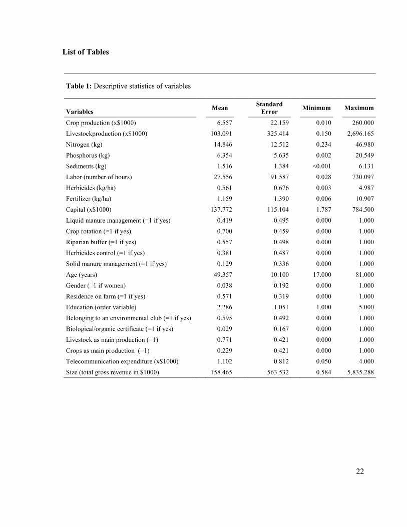
Table 1 presents some descriptive statistics for the variables of interest of this study.

<<< Table 1 about here >>>

5 Results and discussion

5.1 General results

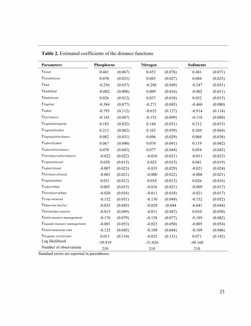
Table 2 presents results obtained from the estimation of the distance functions given by

equation (4) and for phosphorus, nitrogen and sediment. The table allows us to determine the

magnitude and significance of the direct partial elasticities. For the studied pollutants, the first

order coefficients related to “goods” ('^__`) are positive which is expected, as is the negative

first-order estimated coefficients of the “bads” ('a]`). The cross-effect coefficients between

“goods” and “bads” are positive and significant implying a “complementarity” between the two

types of outputs. The similarities in the reported coefficients across pollutants are not surprising

in light of the high degree of correlation between phosphorus, nitrogen and sediments.

13

The coefficients related to crop rotation, solid manure management and belonging to an

environmental club are negative and statistically significant at the 5% level, implying an

upward shift of the environmental frontier. These results indicate that farms that have adopted

these specific BMPs or are member of an environmental club were able to increase their

production while lowering their pollutant runoff. These results are similar to those found by

Tamini (2011) regarding the incidence of advisory/extension activities and those by Tamini et

al (2012) about the impact of BMPs. The coefficients of the remaining management variables

are not significant at 5%.


As presented in Table 3, the first-order elasticity of the “bad” is negative, while it is

positive for the “goods”, reflecting the fact that, at the sample mean, the distance functions are

non-increasing in the “bad” and non-decreasing in the “goods”. The relatively low values of

the substitutability between the “bad” and the “goods” relative to those reported by Custa et al.,

(2009) indicate that policies for controlling the production of a “bad” through the use of

reduction targets or quotas are likely to be effective.12 At -6.038, the substitutability between

nitrogen and the “goods” is the lowest, indicating a lower opportunity cost (See Table 3).

12 For high values (50 to 200 in absolute value), Cuesta et al (2009: p. 2239) concluded that « … economic incentives aimed at attaining an efficient control of pollution by way of taxes, or permits related to “cap and trade”

schemes, as well as incentives to invest in cleaner production technologies, are favored by economic regulators

worldwide.». In our study, regulated pollution reductions would also bring about reductions in good outputs, but nor nearly of the same order.

14

Because 77.1% of the farms included in our data had livestock as their main production, the

higher opportunity cost (and complementarity) for phosphorus was expected.


When statistically significant, the first-order elasticities of input are negative (see Table

4) reflecting the fact that, at the sample mean the distance function are non-increasing in input,

an outcome that is consistent with a theoretical property of distance functions. For the 3

pollutants considered in this study, the first order-elasticity is highest for labor.


As mentioned before, negative (positive) second order elasticity indicates that inputs

are complements (substitutes). Our results indicate that capital and labor tend to be substitutes,

as are capital and fertilizers. The second order elasticities regarding fertilizers and labor are

consistently non-significant. Increasing the use of labor does not seem to have an impact on the

marginal effect of fertilizers and vice-versa.

5.2 Environmental efficiencies

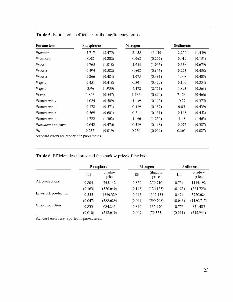
The coefficients related to farm size are statistically different from zero at the 5% level, but in

a non-monotonic way (Table 5). Farms belonging in group 3 are more efficient than those in

group 4 (the reference group), while there is no difference between groups 1, 2 and 3. When

significant, advancing in age has a positive impact on efficiency. This is the case for phosphorus

and sediments for producers in the third class when compared to the reference group, class 1.

The impact is higher when the bad is phosphorus. The positive sign of the coefficient for the

15

crop variable indicates that farms that have crop production as their main production are less

efficient, which is particularly the case for the inefficiency term for sediments. In contrast,

residence on the farm reduces the inefficiency term for sediments, while it has no impact when

the bads are phosphorus and nitrogen. Intuitively, highly educated producers should have an

advantage in terms of acquisition and assimilation of new information. The results in Table 5

suggest that there is no significant gain in environmental efficiency beyond a high school

diploma.

<<< Table 5 about here>>>

The empirical distributions of the environmental efficiency scores for the three bads are

displayed in Figure 1. Table 6 shows that mean efficiency is lowest for sediments, at 0.736,

while mean environmental efficiency for phosphorus and nitrogen are 0.804 and 0.820

respectively. The distribution of efficiency scores for phosphorus displays higher dispersion

than that for nitrogen, but less than that for sediments.

<<< Figure 1 about here >>>


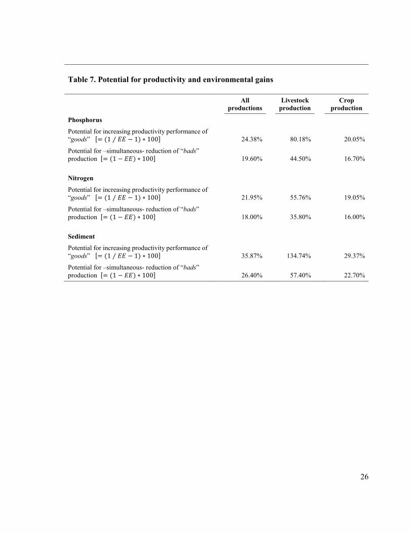
Like Tamini et al (2012), the mean environmental efficiency statistic is lower for farms whose

main source of revenues is livestock production. This is true across all three bads. This

suggests that allocating relatively more resources to extension services targeting livestock

production could be a cost-effective strategy to improve the productivity performance of

16

“goods”, especially for phosphorus and sediments (see Table 7).13 As indicated in Table 7, there

is a potential for increasing productivity, while simultaneous reducing the production of “bads”.

Farms can increase productivity in the production of “goods” by 24.38%, while simultaneously

reducing phosphorus runoff by 19.60%. The policy implication of this result is that higher

agricultural productivity – and higher production levels – can be achieved while reducing

discharges of pollutants in streams, lakes and river. Higher agricultural productivity and output

levels need not simultaneously reduce water quality.


5.3 Shadow prices of the “bads”

Our calculations of shadow prices are reported in Table 6. The average shadow price related to

the emission of a kilogram of phosphorus is $745.142 CAN. This shadow price is interpreted

as the value of total production (animal and plant) to be sacrificed in order to reach the

efficiency frontier (Färe et al, 2005). Tamini et al (2012) found that a 10% reduction in

phosphorus runoff costs on average $461.24 CAN. Using their reported mean for phosphorus,

we can compute an implied price of phosphorus runoff of $725.905 CAN/kg which is close to

our estimate. The shadow price is lower for nitrogen, with a value of $259.72 CAN/kg, while

it is higher for sediments, at $1,114.19 CAN/kg. Ghazalian et al (2010) found that the average

cost associated with a 10% reduction in nitrogen emissions was $324.10 CAN, which is

13 The mean efficiency statistics in this study are higher than those found in Tamini et al (2012) Their mean environmental efficiency statistics for crops and livestock are 0.504 and 0.380. Murty, Kumar and Paul (2006) obtained an average environmental efficiency of 0.853 for Indian sugar companies and Lansink and Reinhard (2004) reported a mean efficiency of 86% for Dutch hog farms producing excess phosphorus and ammonia.

17

equivalent to a cost of $218.25 CAN/kg. Shadow costs are higher for farms primarily involved

in livestock production, for all three “bads”. This is not so surprising because environmental

regulations pertaining to livestock productions in Quebec were tightened in the wake of a

moratorium on hog production imposed in 2002 and lifted in 2005. If the regulations were

significantly stricter, then there would have been less room for heterogeneity in environmental

efficiency amongst livestock producers.

6 Conclusion

The study has evaluated environmental efficiencies of agricultural producers of the Chaudière

watershed in Québec by following the approach proposed by Cuesta et al (2009) featuring the

hyperbolic distance function. Three “bad-specific” distance functions were estimated to

measure environmental performance indices for phosphorus, nitrogen and sediments runoffs.

Environmental efficiency was decomposed in terms of farms characteristics and producers

sociodemograhic attributes. Our results show that farm size, age group, type of production and

on-farm residence each had an impact on environmental inefficiencies. Mean efficiency was

lower for all three “bads” for farms deriving their revenues mainly from livestock production.

For these farms, there is much room to increase productivity in the production of agricultural

“goods” while decreasing the “bads” by-product. This is especially true for phosphorus and

sediment. Overall, there is a potential for increasing productivity while simultaneous reducing

the production of “bads”. The corollary to this result is that policies that require agricultural

producers to reduce the negative by-products of their agricultural activities on water quality do

not necessarily reduce their productivity.

18

The relatively low values of the substitutability between each “bads” and the “goods”

indicate that regulations directly controlling the production of “bads”, like reduction targets or

quotas, are likely to be effective. However, reducing “bads” is more costly for some farms than

others. The shadow costs associated with the reduction of “bads” were consistently higher

across “bads” for farms deriving most of their farm income from crop production.

References

Agriculture et Agroalimentaire Canada [AAC]. 2000. Les meilleures pratiques de gestion agricoles. http://www.agr.gc.ca/pfra/water/agribtm.pdf. Accessed January 31, 2012.

Aigner, D. J., Lovell, C.A.K. and P.J. Schmidt. 1977. Formulation and Estimation of Stochastic Frontier Production Function Models. Journal of Econometrics 6(1): 21-37.

Atkinson, S.E. and J.H. Dorfman. 2005. Bayesian Measurement of Productivity and Efficiency in the Presence of Undesirable Outputs: crediting electric utilities for reducing air pollution. Journal of Econometrics 126(2): 445-468.

Bureau d’Audiences Publiques pour l’Environnement [BAPE]. 2003. Les préoccupations et les propositions de la population au regard de la production porcine, Consultation publique sur le développement durable de la production porcine au Québec, Rapport d’enquête et d’audience publique, Rapport 179. Disponible au : http ://www.bape.gouv.qc.ca (consulté le 08 Juin 2014).

Battese, G. E. 1992. Frontier Production Functions and Technical Efficiency: A Survey of Empirical Applications in Agricultural Economics. Agricultural Economics 7(3) : 185-208.

Boutin, D. 2004. Réconcilier le soutien à l’agriculture et la protection de l’environnement : Tendances et perspectives. Conférence présentée dans le cadre du 67e

Congrès de l’Ordre des agronomes du Québec « Vers une politique agricole visionnaire ».

Chih-Ching, Y., Ching-Kai, H and Y. Ming-Miin. 2008. Technical Efficiency and Impact of Environmental Regulations in Farrow-to-Finish Swine Production in Taiwan. Agricultural Economics 39(1): 51-61.

Coelli, T.S., Rao, D.S.P., O’Donnell, C.J. and G.E. Battese. 2005. An Introduction to Efficiency and Productivity Analysis. Second Edition. Springer.

Cuesta, R.A., Lovell, C.A.K. and J.L. Zofìo. 2009. Environmental Efficiency Measurement with Translog Distance Functions: A Parametric Approach. Ecological Economics 68(8): 2232-2242.

19

Färe, R., Grosskopf, S., Noh, D.-W. and W.L. Weber. 2005. Characteristics of a Polluting Technology: Theory and Practice. Journal of Econometrics 126(2): 469–492.

Farrell, M.J. 1957. The Measurement of Productive Efficiency. Journal of the Royal Statistical Society 120: 253-290.

Fernandez, C., Koop, G. and M.F.J. Steel. 2000. A Bayesian analysis of multiple-output production frontier. Journal of Econometrics 98(1): 47–79.

Fernandez, C., Koop, G. and M.F.J. Steel. 2002. Multiple-output production with undesirable outputs: an application to nitrogen surplus in agriculture. Journal of American Statistical Association 97: 432–42.

Galanapoulos, K., Aggelopoulos, S., Kamenidou, I. and K. Mattas. 2006. Assessing the Effects of Managerial and Production Practices on the Efficiency of Commercial Pig Farming. Agricultural Systems 88(2): 125-141.

Gangbazo, G. and A. Le Page. 2005. Détermination d’objectifs relatifs à la réduction des charges d’azote, de phosphore et de matières en suspension dans les bassins versants prioritaires. Direction des politiques de l’eau, Bureau de la gestion par bassin versant, Ministère du Développement durable, de l’Environnement et des Parcs, Québec, EnvirodocENV/2005/0215. http://www.mddep.gouv.qc.ca/eau/bassinversant/reduction.pdf. Accessed June 16, 2014.

Ghazalian, P.L., Larue, B. and G.E West. 2009. Best management practices to enhance water quality: who is adopting them? Journal of Agricultural and Applied Economics 41(3): 663–682.

Ghazalian, P.L., Larue, B. and G.E West. 2010. Best Management Practices and the Production of Good and Bad Outputs. Canadian Journal of Agricultural Economics 58(3): 283-302.

Korol, M. 2002. Canadian Fertilizer Consumption, Shipments and Trade. Agriculture and Agrifood Canada (AAC). http://www.cfi.ca/files/publications/statistical_documents/cf01_02_e.pdf. Accessed June 11, 2014.

Lansink, A.O. and S. Reinhard. 2004. Investigating Technical Efficiency and Potential Technological Change in Dutch Pig Farming. Agricultural Systems 79(3): 353-367.

Lau, L.J. 1972. Profit Functions of Technologies with Multiple Inputs and Outputs. Review of Economics and Statistics 54(3): 281-289.

Manello, A. 2012. Efficiency and productivity analysis in presence of undesirable output: an extended literature review. Efficiency and productivity in presence of undesirable outputs, 15.

Manello, A. 2013. Productivity and efficiency analysis in presence of pollution: a review of non-parametric methods. World Review of Science, Technology and Sustainable

development 10(4): 242-262.

20

Martel, S., Seydoux, S., Michaud, A. and I. Beaudin. 2006. Évaluation des effets combinés des principales pratiques de gestion bénéfiques (PBG). Revue de littérature et schéma décisionnel pour la mise en œuvre de PGB. Document rédigé dans le cadre de l’INENA (Initiative nationale d’élaboration de normes agroenvironnementales). Institut de Recherche et de Développement en Agroenvironnement (IRDA).

Michaud, A., I. Beaudin, J. Deslandes, F. Bonn and C.A. Madramootoo. 2006. Variabilité spatio-temporelle des flux de sédiments et de phosphore dans le bassin versant de la rivière aux Brochets, au sud du Québec. Partie II : Évaluation de l’effet de scénarios agroenvironnementaux alternatifs à l’aide de SWAT. Agrosolutions 17, 21-32.

Morrison-Paul, C.J., Johnston, W.E. and G.A. Frengley. 2000. Efficiency in New Zealand sheep and beef farming: The impacts of regulatory reform. Review of Economics and Statistics 82(2): 325-337.

Mosheim, R. and C.A.K. Lovell. 2009. Scale Economies and Inefficiency of U.S. Dairy Farms. American Journal of Agricultural Economics 91(3): 777-794.

Murty, M.N., Kumar, S. and M. Paul. 2006. Environmental Regulation, Productive Efficiency and Cost Pollution Abatement: a Case Study of the Sugar Industry in India. Journal of Environmental Management 79(1): 1-9.

Paul, C.J.M. and R. Nehring. 2005. Product Diversification, Production Systems, and Economic Performance in U.S. Agricultural Production. Journal of Econometrics 126(2): 525-548.

Reinhard, S., Lowell, C.A.K. and G. Thijssen. 1999. Econometric Estimation of Technical and Environmental efficiency: An Application to Dutch Dairy Farms. American Journal of Agricultural Economics 81(1): 44-60.

Reinhard, S. and G. Thijssen. 2000. Nitrogen Efficiency of Dutch Dairy Farms: a Shadow Cost System Approach. European Review of Agricultural Economics 27(2): 167-186.

Rousseau, A.N., Savary, S., Hallema, D.W., Gumiere, S.J. and É. Foulon. 2013. Modeling the effects of agricultural BMPs on sediments, nutrients, and water quality of the Beaurivage River watershed (Quebec, Canada). Canadian Water Resource Journal 38(2): 99-120.

Singbo, A.G. and B. Larue. 2015. Scale economies, technical efficiency and the sources of total factor productivity growth of Quebec dairy farms. In press Canadian Journal of Agricultural Economics.

Singbo A.G. and A.O. Lansink. 2010. Lowland farming system inefficiency in Benin (West Africa): directional distance function and truncated bootstrap approach. Food Security, 2(4): 367–382.

Tamini, L.D. 2011. A Nonparametric Analysis of the Impact of Agri-environmental Advisory Activities on Best Management Practice Adoption: A Case Study of Québec. Ecological Economics 70(7): 1363-1374.

Tamini, L.D. and B. Larue. 2012. La durabilité environnementale de la filière porcine au Québec et au Manitoba : le moratoire est-il un passage obligatoire? Dans Les politiques des

21

ressources naturelles - le Québec comparé. Sous la direction de J. Crête. Les Presse de l'Université Laval.

Tamini, L.D., Larue, B. and G. West. 2012. Technical and environmental efficiencies and best management practices in agriculture. Applied Economics 44(13): 1659-1672.

Yélou, C., Larue, B. and K.C. Tran. 2010. Threshold Effects in Panel Data Stochastic Frontier Models of Dairy Production in Canada. Economic Modelling 27(3): 641-647.

22

List of Tables

Table 1: Descriptive statistics of variables

Variables

Mean

Standard

Error Minimum Maximum

Crop production (x$1000) 6.557 22.159 0.010 260.000

Livestockproduction (x$1000) 103.091 325.414 0.150 2,696.165

Nitrogen (kg) 14.846 12.512 0.234 46.980

Phosphorus (kg) 6.354 5.635 0.002 20.549

Sediments (kg) 1.516 1.384 <0.001 6.131

Labor (number of hours) 27.556 91.587 0.028 730.097

Herbicides (kg/ha) 0.561 0.676 0.003 4.987

Fertilizer (kg/ha) 1.159 1.390 0.006 10.907

Capital (x$1000) 137.772 115.104 1.787 784.500

Liquid manure management (=1 if yes) 0.419 0.495 0.000 1.000

Crop rotation (=1 if yes) 0.700 0.459 0.000 1.000

Riparian buffer (=1 if yes) 0.557 0.498 0.000 1.000

Herbicides control (=1 if yes) 0.381 0.487 0.000 1.000

Solid manure management (=1 if yes) 0.129 0.336 0.000 1.000

Age (years) 49.357 10.100 17.000 81.000

Gender (=1 if women) 0.038 0.192 0.000 1.000

Residence on farm (=1 if yes) 0.571 0.319 0.000 1.000

Education (order variable) 2.286 1.051 1.000 5.000

Belonging to an environmental club (=1 if yes) 0.595 0.492 0.000 1.000

Biological/organic certificate (=1 if yes) 0.029 0.167 0.000 1.000

Livestock as main production (=1) 0.771 0.421 0.000 1.000

Crops as main production (=1) 0.229 0.421 0.000 1.000

Telecommunication expenditure (x$1000) 1.102 0.812 0.050 4.000

Size (total gross revenue in $1000) 158.465 563.532 0.584 5,835.288

23

Table 2. Estimated coefficients of the distance functions

Parameters Phosphorus Nitrogen Sediments

'^__` 0.481 (0.067) 0.453 (0.076) 0.481 (0.071) '^__`b^__` 0.070 (0.023) 0.083 (0.027) 0.084 (0.025) 'a]` -0.256 (0.037) -0.288 (0.049) -0.247 (0.051) 'a]`ba]` -0.002 (0.008) 0.009 (0.016) -0.002 (0.011) 'a]`b^__` 0.026 (0.012) 0.037 (0.018) 0.032 (0.015) 'c]d1e]@ -0.384 (0.077) -0.271 (0.085) -0.460 (0.080) 'f]F_g -0.793 (0.112) -0.635 (0.127) -0.914 (0.114) 'hTge1@15Tg6 -0.145 (0.087) -0.152 (0.099) -0.118 (0.088) 'c]d1e]@bc]d1e]@ 0.183 (0.032) 0.144 (0.031) 0.212 (0.033) 'c]d1e]@bf]F_g 0.212 (0.062) 0.162 (0.059) 0.269 (0.064) 'c]d1e]@bhTg1@15Tg6 0.082 (0.031) 0.096 (0.029) 0.068 (0.036) 'f]F_gbf]F_g 0.067 (0.040) 0.074 (0.041) 0.119 (0.042) 'f]F_gbhTge1@15Tg6 0.070 (0.043) 0.077 (0.044) 0.054 (0.043) 'hTge1@15Tg6bhTge1@15Tg6 -0.022 (0.022) -0.016 (0.021) -0.011 (0.023) 'c]d1e]@b^__` 0.038 (0.015) 0.025 (0.015) 0.041 (0.019) 'f]F_gb^__` -0.007 (0.023) -0.035 (0.029) -0.021 (0.024) 'hTge@15Tg6b^__` -0.001 (0.021) -0.000 (0.022) -0.006 (0.021) 'c]d1e]@ba]` 0.031 (0.012) 0.034 (0.013) 0.026 (0.016) 'f]F_gba]` 0.005 (0.015) -0.016 (0.021) -0.009 (0.017) 'hTge1@15Tg6ba]` -0.020 (0.016) -0.011 (0.018) -0.021 (0.017) 'cg_dg_e]e1_/ -0.152 (0.051) -0.130 (0.049) -0.152 (0.052) 'i1d]g1]/Fj&&Tg -0.035 (0.045) -0.029 (0.044 -0.041 (0.044) 'kTgF1l1`T6l_/eg_@ -0.013 (0.049) -0.011 (0.047) 0.010 (0.050) 'm_@1`-]/jgT-]/]nT-T/e -0.176 (0.079) -0.158 (0.077) -0.189 (0.082) 'f1+j1`T-]/jgT-]/]nT-T/e -0.001 (0.053) -0.023 (0.050) -0.005 (0.054) '�/o1g_/-T/e]@l@jF -0.125 (0.045) -0.109 (0.044) -0.109 (0.046) 'pgn]/1llTge1&1l]eT 0.011 (0.134) -0.025 (0.131) 0.071 (0.142) Log likelihood -39.919 -31.826 -49.160 Number of observations 210 210 210

Standard errors are reported in parentheses.

24

Table 3. Substitutability between “goods” and “bads”

Phosphorus

Nitrogen

Sediment

First order elasticity of the “goods” (qrss) 0.778 0.782 0.770

First order elasticity of the “bads” (qtss) -0.112 -0.129 -0.110

Substitutability between “goods” and “bads” (ur.tss ) -6.926 -6.038 -6.984

Table 4. Estimated inputs elasticities

Phosphorus Capital Labor Fertilizers

Estimated coefficients �'-� -0.384 (0.077) -0.793 (0.112) -0.145 (0.087)

First order elasticities �=-�� 0.046 (0.054) -0.639 (0.074) -0.050 (0.049)

Second order elasticities D-,@�� #

Capital 0.231 (0.053) 0.268 (0.102) 0.104 (0.051)

Labor 0.357 (0.124) 0.113 (0.081) 0.117 (0.086)

Fertilizers -0.039 (0.031) -0.033 (0.043) 0.010 (0.022)

Nitrogen Capital Labor Fertilizers




Capital 0.182 (0.051) 0.205 (0.097) 0.121 (0.048)

Labor 0.274 (0.118) 0.125 (0.083) 0.130 (0.089)

Fertilizers -0.046 (0.029) -0.037 (0.044) 0.007 (0.022)

Sediments Capital Labor Fertilizers




Capital 0.268 (0.055) 0.340 (0.106) 0.086 (0.059)

Labor 0.453 (0.129) 0.201 (0.084) 0.091 (0.086)

Fertilizers -0.033 (0.036) -0.026 (0.043) 0.005 (0.024) Standard errors are reported in parentheses. These elasticities are obtained from the Delta method. They are reported at their respective average.

25

Table 5. Estimated coefficients of the inefficiency terms

Parameters Phosphorus Nitrogen Sediments

O^T/`Tg -2.717 (2.475) -3.155 (3.040 -2.256 (1.449)

OvT@Tl_- -0.08 (0.202) -0.068 (0.207) -0.019 (0.151) Om15T_� -1.765 (1.018) -1.944 (1.035) -0.658 (0.679) Om15T_. -0.494 (0.582) -0.608 (0.615) -0.223 (0.458) Om15T_X -1.266 (0.484) -1.075 (0.481) -1.008 (0.405) OxnT_. -0.451 (0.418) -0.501 (0.429) -0.109 (0.354) OxnT_X -3.96 (1.959) -4.472 (2.751) -1.893 (0.563) Ocg_d 1.825 (0.547) 1.135 (0.624) 2.124 (0.466) O�`jl]e1_/_. -1.024 (0.509) -1.139 (0.515) -0.77 (0.375) O�`jl]e1_/_X -0.178 (0.571) -0.329 (0.587) 0.05 (0.439) O�`jl]e1_/_S -0.569 (0.601) -0.711 (0.591) -0.168 (0.452) O�`jl]e1_/_Z -1.722 (1.362) -1.196 (1.230) -1.68 (1.463) OiT61`T/lT_/&]g- -0.642 (0.476) -0.529 (0.468) -0.975 (0.387)

yj 0.235 (0.019) 0.230 (0.019) 0.203 (0.027)


Table 6. Efficiencies scores and the shadow price of the bad

Phosphorus Nitrogen Sediment

EE

Shadow price

EE Shadow price

EE Shadow price

All productions 0.804 745.142 0.820 259.716 0.736 1114.192 (0.163) (320.040) (0.148) (126.153) (0.183) (264.723) Livestock production 0.555 1290.329 0.642 1317.133 0.426 3720.684 (0.047) (388.629) (0.041) (590.708) (0.048) (1180.717) Crop production 0.833 684.243 0.840 135.976 0.773 821.485

(0.010) (312.010) (0.009) (70.535) (0.011) (245.944)


26

Table 7. Potential for productivity and environmental gains

All

productions

Livestock

production

Crop

production

Phosphorus

Potential for increasing productivity performance of “goods” z= �1 ⁄ {{ − 1� ∗ 100�

24.38% 80.18% 20.05%

Potential for –simultaneous- reduction of “bads” production z= �1 − {{� ∗ 100�

19.60% 44.50% 16.70%

Nitrogen


21.95% 55.76% 19.05%


18.00% 35.80% 16.00%

Sediment


35.87% 134.74% 29.37%


26.40% 57.40% 22.70%

27

List of figures

Figure 1. Predicted environmental efficiencies distribution

0

.05

.1

.15

.2

.25

Fraction

.2 .4 .6 .8 1Environmental efficiency

Prosphorus

0

.05

.1

.15

.2

Fraction

.2 .4 .6 .8 1Environmental efficiency

Nitrogen

0

.05

.1

.15

.2

Fraction

0 .2 .4 .6 .8 1Environmental efficiency

Sediment

Agricultural production and pollutant runoffs in Québec’s ... · 2 Agricultural production and...

Documents

Transcript of Agricultural production and pollutant runoffs in Québec’s ... · 2 Agricultural production and...