AGRIBALYSE : METHODOLOGY - Changement … Koch, Agroscope Technical coordination: Vincent Colomb,...
333
Technical coordination: Vincent Colomb, Service Agriculture et Forêts- Direction Production et Energies Durables – ADEME Angers © 2015 ADEME AGRIBALYSE ® : METHODOLOGY Version 1.3 November 2016 Authors Peter Koch, Agroscope Thibault Salou, INRA Co-Authors Vincent Colomb (ADEME), Sandra Payen (CIRAD), Sylvain Perret (CIRAD) Aurélie Tailleur (ARVALIS), Sarah Willmann (ARVALIS) FINAL REPORT
Transcript of AGRIBALYSE : METHODOLOGY - Changement … Koch, Agroscope Technical coordination: Vincent Colomb,...

Technical coordination: Vincent Colomb, Service Agriculture et Forêts- Direction Production et Energies Durables – ADEME Angers
© 2015 ADEME
AGRIBALYSE®: METHODOLOGY
Version 1.3
November 2016
Authors
Peter Koch, Agroscope Thibault Salou, INRA
Co-Authors
Vincent Colomb (ADEME), Sandra Payen (CIRAD), Sylvain Perret (CIRAD) Aurélie Tailleur (ARVALIS), Sarah Willmann (ARVALIS)
Étude réalisée pour le compte de l'ADEME par RDC-Environnement
Coordination technique : Sylvain PASQUIER – Département Organisation des
Filières et Recyclage - Direction des Déchets et Sols – ADEME Angers
FINAL REPORT

AGRIBALYSE
®: Methodology 2
CONTRIBUTING AUTHORS
• Vincent Colomb, ADEME – Co-Author
Abstract and general editorial, updating v1.1, v1.2 and v1.3 with support of Peter Koch, Koch consulting
• Anne Paillier, ADEME – Co-Author
Part C: Impact assessment Appendix E: Changes in soil carbon stocks
• Sandra Payen, CIRAD – Co-Author
Appendix F: Accounting for water in LCA
Sylvain Perret, CIRAD – Co-Author Chapter B.2.4: Direct emissions from paddy fields Appendix D: Setting model parameters for paddy field emissions in all datasheets
• Aurélie Tailleur and Sarah Willmann ARVALIS – Co-Authors
Chapter B.2.4.7: Nitrate emissions Chapter B.3.3: Allocating processes, inputs and outputs for cropping sequences Appendix D: Setting model parameters - datasheet 8
Please cite this report as
Koch P. and Salou T. 2016. AGRIBALYSE®: Rapport Méthodologique – Version 1.3. November 2016.
Ed ADEME. Angers. France. 332 p.

AGRIBALYSE
®: Methodology 3
EDITORS
All members of the AGRIBALYSE® Steering Committee (in alphabetical order)
• Samy Ait Amar, ACTA
• Claudine Basset-Mens, CIRAD
• Yannick Biard, INRA
• Hervé Bossuat, ACTA
• Michel Cariolle, ITB
• Sonia Clermidy, IFV
• Vincent Colomb, ADEME
• Sylvie Dauguet, TERRES INOVIA
• Sandrine Espagnol, IFIP
• Francis Flénet, TERRES INOVIA
• Armelle Gac, Institut de l‘Elevage
• Gérard Gaillard, Agroscope
• Dominique Grasselly, Ctifl
• Sébastien Kerner, IFV
• Peter Koch, Agroscope
• Afsaneh Lellahi, ARVALIS
• Elise Lorinquer, Institut de l‘Elevage
• Romain Manceau, Astredhor
• Muriel Millan, Ctifl
• Jérôme Mousset, ADEME
• Anne Paillier, ADEME
• Sandra Payen, CIRAD
• Sylvain Perret, CIRAD
• Paul Ponchant, ITAVI
• Olivier Réthoré, ADEME
• Thibault Salou, INRA
• Anne Schneider, TERRES INOVIA
• Aurélie Tailleur, ARVALIS
• Thierry Tran, CIRAD
• Hayo van der Werf, INRA
• Sarah Willmann, ARVALIS
Translation by Tony Tebby, e-mail: [email protected]

AGRIBALYSE
®: Methodology 4
ACKNOWLEDGEMENTS
We should like to thank the following for their contributions to the development of the
methodology, to building Life Cycle data sets and to checking the quality of crop production
system data.
Thierry Boulard, INRA
Emmanuelle Garrigues, INRA
Marilys Pradel, IRSTEA
Phillipe Roux, IRSTEA
Virignie Parnaudeau, INRA
Jacques Agabriel, INRA
Nourraya Akkal, INRA
Marc Benoit, INRA
Amandine Berthoud, InVivo
AgroSolutions
Joachim Boissy, Agro-Transfert
Ressources et Territoires
Dylan Chevalier, Chambre régionale
d'Agriculture Pays de la loire
Katell Crépon, Coop de France
Elodie Dezat, Chambre régionale
d’Agriculture régionale de Bretagne
Nathalie Dupont, Institut Français des
Productions Cidricoles
Catherine Experton, ITAB
Philippe Faverdin, INRA
Laetitia Fourrié, ITAB
Laurence Fontaine, ITAB
Pierre Garsi, Lycée professionnel de
Guérande
Pierre Glerant, Sileban
Caroline Godard, Agro-Transfert
Ressources et Territoires
Anne Guerin, Institut Français des
Productions Cidricoles
Eric Hostalnou, Chambre d'agriculture
des Pyrénées Orientales
Côme Isambert, ITAB
Benoît Jeannequin, Montpellier
SupAgro
Frédérique Jourjon, ESA
Claver Kanyarushoki, ESA
Pauline Maupu, InVivo AgroSolutions
Fréderic Rey, ITAB
Tony Tebby, Translator
Marie Thiollet-Scholtus, INRA
Jean-Pierre Vandergeten, IRBAB
As well as all those experts who wished to remain anonymous.
All rights reserved. This report may not be reproduced in whole or in part without the consent of the authors or copyright holder. The report may be copied or reproduced strictly for private use and parts may be reproduced for analyses and short quotations in critical, educational or informative publications.

AGRIBALYSE
®: Methodology 5
THE AGRIBALYSE® PROGRAM
Methodology
Table of contents
Table of contents ......................................................................................................................... 5
Abstract 8
Résumé 11
Abbreviations ............................................................................................................................ 15
Introduction .............................................................................................................................. 18
Part A – Defining the aims and scope of the study ................................................................. 19
A.1 Aims....................................................................................................................................... 19
A.1.1 The AGRIBALYSE® program and background to this report ........................................ 19
A.1.2 Aims of the AGRIBALYSE® program ............................................................................. 20
A.1.3 Deliverables ................................................................................................................. 20
A.1.4 Users of the results from the AGRIBALYSE® program ................................................. 21
A.2 Scope ..................................................................................................................................... 21
A.2.1 Product systems studied and their functions.............................................................. 22
A.2.2 System boundaries ...................................................................................................... 26
A.2.3 Data requirements ...................................................................................................... 37
A.2.4 Data quality requirements .......................................................................................... 39
A.2.5 Type of critical review – Quality control ..................................................................... 44
A.2.6 Type and format of the report required for the study ................................................ 47
Part B – LCI data sets ............................................................................................................ 49
B.1 Data collection procedures and systems used for AGRIBALYSE® ......................................... 49
B.2 Data collection ...................................................................................................................... 49

AGRIBALYSE
®: Methodology 6
B.2.1 Data collection............................................................................................................. 49
B.2.2 Input data categories .................................................................................................. 50
B.3 Calculating the LCI data sets ................................................................................................. 52
B.3.1 Data processing applications ....................................................................................... 52
B.3.2 Relating data to the functional units ........................................................................... 53
B.3.3 Calculating the LCI data sets of inputs for agricultural production ............................ 53
B.3.4 Transport of inputs ...................................................................................................... 59
B.3.5 Calculation models for the consumption of resources and direct emissions from
polluting substances ..................................................................................................................... 61
B.4 Allocation of flows and emissions ......................................................................................... 78
B.4.1 Allocation of shared inputs: infrastructure ................................................................. 78
B.4.2 Allocation to co-products ............................................................................................ 78
B.4.3 Allocation of processes, inputs and outputs for cropping sequences ........................ 86
Part C – Impact assessment .................................................................................................. 89
Part D – Conclusion ............................................................................................................... 93
Bibliography .............................................................................................................................. 94
Glossary 102
Appendices 112

AGRIBALYSE
®: Methodology 7
Appendices
Appendix A: Product groups and variants in the AGRIBALYSE program ...................................... 113
Appendix B: Calculating national LCI data sets (French average) ................................................ 127
Appendix C: Specification for quality control of production system data collected for the
AGRIBALYSE program ....................................................................................... 134
Appendix D: Parameters for models for calculating direct emissions used in the AGRIBALYSE
program ........................................................................................................... 150
Datasheet 1: Ammonia (NH3) ........................................................................................... 150 Datasheet 2: Excretion of nitrogen by livestock ................................................................ 159 Datasheet 3: Carbon dioxide (CO2) ................................................................................... 163 Datasheet 4: Trace metals ................................................................................................ 165 Datasheet 5: Soil loss ....................................................................................................... 173 Datasheet 6: Combustion emissions ................................................................................. 180 Datasheet 7: Methane (CH4) ............................................................................................ 182 Datasheet 8: Nitric oxide (NO) ......................................................................................... 195 Datasheet 9: Nitrate emissions (NO3-) ............................................................................. 198 Datasheet 10: Land occupation (m2.yr) and transformation (m2) ....................................... 212 Datasheet 11: Phosphorus emissions (P) .......................................................................... 214 Datasheet 12: Dinitrogen oxide (N2O)............................................................................... 222 Datasheet 13: Active substances in pesticides .................................................................. 229 Datasheet 14: Emissions from fish farms .......................................................................... 231 Datasheet 15: Extrapolation of seed and plant LCI data sets ............................................. 233 Datasheet 16: Use of “Animal of 0 day” LCIs for initiating animal systems ......................... 237 Datasheet 17: Allocation of P and K fertilizers and organic N fertilizer within cropping
sequences................................................................................................ 239 Datasheet 18: Meteorological data for calculating Thai rice emissions .............................. 245
Appendix E: Changes in soil carbon stocks ................................................................................ 246
Appendix F: Taking account of water in Life Cycle Assessments ................................................. 255
Appendix G: Assignment of data collection module inputs to ecoinvent LCI data sets ................ 258
Appendix H: Composition of organic fertilizers.......................................................................... 259
Appendix I: Building average fertilizer LCI data sets .................................................................. 262
Appendix J: Building the machinery data sets ........................................................................... 268
Appendix K: Building the agricultural processes ........................................................................ 286
Appendix L: Building the livestock feed processes ..................................................................... 300
Appendix M: Allocations used for AGRIBALYSE ......................................................................... 325

AGRIBALYSE
®: Methodology 8
Abstract
The AGRIBALYSE® program
Farmers, the food industry, policy makers and consumers are increasingly interested in the environmental impacts of food products. In 2009, following the “Grenelle de l’Environnement” organized by the Ministry of the Environment, it was clear that it was necessary to improve the understanding of the environmental impacts of agricultural products and share the resulting data. The French Environment and Energy Management Agency (ADEME) launched the AGRIBALYSE® program to create a Life Cycle Inventory (LCI) database of French agricultural products. This database is restricted to flow LCI data sets and data for life cycle impact assessments (LCIA) rather than full life cycle assessments (LCA), which would require several more steps: normalization, aggregation and interpretation of the results. Many partners contributed to the program, including research institutes (INRA, Agroscope, CIRAD) and Technical Institutes representing the whole of the agricultural industry. AGRIBALYSE® was built with two aims: i) build an LCI database to provide data for environmental labeling of food products and ii) share the data to enable the agricultural and food industries to assess the production chain and reduce environmental impacts. AGRIBALYSE® provides 136 LCI data sets for arable, horticultural and livestock products. The deliverables are:
A database in ecospold_v1 formats. Two Excel files (one for animal production, one for crop production) provided for
AGRIBALYSE v1.2 with LCI and LCIA indicators. A final report in French and English (Agribalyse: Assessment and lessons for the
future, Colomb et al, 2013), describing the project stages and main findings and including two notes on the quality control for the LCI data sets and the results as well as a sample of the sensitivity analysis of the results for two products
The AGRIBALYSE® data collection guide This report on the methodology
This report on the methodology
General aim of the report This document presents the methodologies selected by the 14 partners during the construction of the AGRIBALYSE® database. Most of these were adopted unanimously, the others by a majority vote. In conjunction with the metadata with each LCI data set, this document ensures that the AGRIBALYSE® approach is transparent. It gives a detailed description of the methods selected but is not intended to be a manual. It should help LCA practitioners to assess the quality of the AGRIBALYSE® database and create LCI data sets that are comparable to those of the AGRIBALYSE® database. LCI data set handling: data collection, conversion and calculation

AGRIBALYSE
®: Methodology 9
The data for the production systems was entered by the Technical Institutes using the data collection module (DCM) developed for AGRIBALYSE® using Excel. This module was then coupled to the direct emission calculation models within the inventory data processing system (IDPS), also using Excel, to obtain the direct emission flows. The background processes were then added using Simapro® to obtain the LCI and LCIA data sets. Quality control There were two levels of quality control. The quality of the production system data, entered by the Technical Institutes into the DCM, was checked by independent experts. The LCI data calculated by INRA and Agroscope was checked internally by the Technical Institutes. This two-stage quality control process significantly improved the quality of the LCI data sets. Products assessed AGRIBALYSE® created LCI data sets for the main French agricultural products (and three imported products), using a standardized hierarchy. “Product groups” were generalized products (e.g. wheat, maize, broilers, pigs, etc). The French average LCI data sets for most product groups were built by averaging the individual LCI data sets for varied production systems (e.g., conventional, organic, AOC, regional variants, etc). These average LCI data sets were constructed case by case. Including variations within product groups, the database contains a total of 136 LCI data sets: 80 for livestock production and 57 for arable and horticultural production (Appendix A).
Products inventoried in AGRIBALYSE®
Annual crops Durum wheat, soft wheat, sugar beet, carrots, rapeseed, faba beans, grain maize, barley, peas, potatoes, sunflowers, triticale
Forage/grassland Grass, alfalfa, silage maize
Fruits and vineyard Peaches, apples, cider apples, wine grapes
Special crops Roses, tomatoes, ornamental shrubs
Tropical special crops Coffee, clementines, jasmine rice, cocoa,oil palm fruit, mango
Arable and horticultural total: 28 product groups
Cattle Cow’s milk, beef cattle
Sheep Sheep’s milk, lambs
Goats Goat’s milk
Poultry Eggs, broilers, turkeys, ducks for roasting, ducks for foie gras
Rabbits Rabbits
Aquaculture Trout, sea bass/sea bream
Pigs Pigs
Livestock total: 14 product groups
Representativeness AGRIBALYSE® originally aimed to provide LCI datasets for agricultural products representative of the French market. However, due to the variability of farming practices, soils and climate in France, it was often difficult to construct a realistic “national average” production system. This was one reason for creating several LCI data sets for the same product, for different farming practices or regions. Where possible, they were then averaged to obtain “national average” products but, even so, an LCI data set representative of the whole of France was not possible for all products. Representativeness should always be considered when using the LCI data sets.

AGRIBALYSE
®: Methodology 10
System boundaries (space and time) The system boundaries for the AGRIBALYSE® LCI data sets are from cradle to farm gate. For crops, all up-stream processes (input production) are included but post-harvest operations are excluded, even though they may occur on the farm (e.g., potato storage, cereal drying). For animals, all operations required for the production phase are included (e.g., animal production, fodder storage, milking room and machines) but no processing phase is included (e.g., slaughter, cheese making). To build LCI data sets representative of current production systems, the reference period chosen was from 2005 to 2009. Direct emissions, linked to animal and crop production, on the farm itself were modeled in AGRIBALYSE®, whereas indirect emissions associated with inputs were based on existing data, mainly from ecoinvent®. Additional work was required for indirect emissions associated with some feed ingredients (Appendix L). Models used to calculate direct emissions Farming activities cause direct emissions (e.g., CO2, NH3, trace metals, P, pesticides) and use resources (e.g., water, land). Emissions to environmental compartments (i.e., water, soil, air) were calculated using models. Each emission was calculated using a specific model chosen to be the most suitable for the requirements of the program. Table 15 shows the emissions and resources included, the source and consumers and the models used. Allocation The allocation rules follow international recommendations. For arable and horticultural crops, most co-products are generated in the processing phase, which is not included in AGRIBALYSE®. For livestock production, a “biophysical” allocation method was used. If possible, allocation was avoided by breaking the system down into animal classes, characterized by animal’s age/physiological stage and management. Then, for animal classes requiring allocation (e.g., dairy cows during milk production), allocation was based on the metabolic energy required to produce each co-product (e.g., calf, milk). However, impacts of animal classes producing a single product were allocated 100% to this product. For example, all the impacts of the “dairy heifer” class were allocated to the “cull cow” product.

AGRIBALYSE
®: Methodology 11
Résumé
Le programme AGRIBALYSE®
Les impacts environnementaux des produits agricoles est un sujet qui intéresse de plus en plus les agriculteurs, les filières, les pouvoirs publics et les consommateurs. Suite aux décisions prises dans le cadre du Grenelle de l’Environnement et à la volonté de mutualiser et d’améliorer les connaissances des impacts environnementaux des produits agricoles, l’ADEME a décidé de lancer un programme pour réaliser une base de données (BDD) d’Inventaires de Cycle de Vie (ICV) des produits agricoles, nommée AGRIBALYSE®. Cette base de données se limite à la production d’indicateurs de flux (ICV) et d’impacts (AICV) par opposition à la production d’Analyses du Cycle de Vie (ACV) complète, incluant les étapes de normalisation, d’agrégation et d’interprétation des résultats. Le programme a été monté en collaboration étroite avec les partenaires de la recherche (INRA, Agroscope et CIRAD) et avec les Instituts Techniques des principales filières agricoles. Le but de ce travail est double : i) constitution d’une base de données d’ICV pour renseigner l’affichage environnemental des produits alimentaires ; ii) mutualisation des connaissances pour aider les professionnels du monde agricole et agro-alimentaire dans l’analyse des filières et la réduction de leurs impacts environnementaux. Le programme a permis la mise à disposition de 136 ICV de produits agricoles animaux et végétaux. Les livrables sont :
Une base de données ICV sous format ecospold_v1. Un fichier de synthèse Excel mis à disposition dans la version AGRIBALYSEv1.2
contenant les résultats ICV et IACV. . Un rapport « Bilan et enseignements » (Colomb et al, 2013), présentant le
déroulement et les principaux résultats du programme, et incluant deux notes sur le contrôle qualité des ICV et des résultats ainsi qu’une analyse exemplaire de sensibilité des résultats pour deux productions.
Le guide de collecte « AGRIBALYSE® » (Biard et al, 2011a). Ce rapport méthodologique.
Le rapport méthodologique
Objectif général du rapport Ce rapport documente les choix méthodologiques effectués par les 14 partenaires du programme lors de l’établissement de la base de données AGRIBALYSE®. Ces choix ont été approuvés généralement à l’unanimité, sinon à la majorité. En complément des métadonnées disponibles pour chaque ICV, ce rapport assure la transparence de la démarche. Il présente la démarche et les choix retenus mais n’est pas conçu comme un guide de préconisation. Il doit permettre à des personnes extérieures d’évaluer la qualité des données fournies et de réaliser des ICV comparables à celles d’AGRIBALYSE®. Calcul des ICV : données collectées, chaine de traitement Les données d’inventaires décrivant les itinéraires techniques ont été saisies par les instituts techniques dans l’Outil Informatique de Saisie (OIS), développé pour AGRIBALYSE® sous Excel. L’OIS a ensuite été couplé à l’ensemble des modèles de calcul des émissions directes

AGRIBALYSE
®: Methodology 12
au sein de la chaine de traitement des données (CDT), développée également sous Excel. Le couplage des données d’inventaires avec les modèles a permis d’obtenir les flux d’émissions directs. Les processus d’arrière plan indirects ont ensuite été intégrés via Simapro®, ce qui a permis le calcul des ICV et AICV. Contrôle qualité Un contrôle qualité des données a été réalisé à deux niveaux. Dans un premier temps, les données d’itinéraires techniques, renseignées par les Instituts Techniques dans l’OIS, ont été contrôlées par des experts extérieurs au programme AGRIBALYSE®. Dans un deuxième temps, les données ICV calculées par l’INRA et Agroscope ont été contrôlées en interne par les instituts techniques. Ce double contrôle a permis d’améliorer significativement la qualité des inventaires produits. Produits étudiés AGRIBALYSE® a permis de réaliser l’ICV des principaux produits agricoles français (et trois produits importés), selon une méthodologie homogène. Les « groupes de produits » font références aux cultures ou aux animaux (ex : blé, maïs, poulet de chair, porc, etc.). La construction d’ICV représentatifs France pour la plupart des « groupe de produits » s’est faite en agrégeant des ICV unitaires correspondants à des systèmes contrastés (conventionnel, biologique, AOC, déclinaisons régionales, etc.). Cette agrégation s’est faite au cas par cas pour chaque production. En tenant compte des déclinaisons (systèmes de productions spécifiques), la base de données contient au total 136 ICV : 80 ICV de productions animales et 57 de productions végétales (Annexe A).
Les produits étudiés dans AGRIBALYSE® Cultures annuelles Blé dur, blé tendre, betterave sucrière, carotte, rapeseed,
féverole, maïs, orge, pois, pomme de terre, tournesol, triticale Prairies/Fourrages Herbe, luzerne, maïs ensilage
Fruits et vigne Pêche/nectarine, pomme, pomme à cidre, raisin de cuve* Cultures spéciales métropolitaines Rose, tomate, arbuste Cultures spéciales tropicales Coffee, clémentine, riz jasmin, mangue, cacao, fruit du palmier à
huile Production végétale : 28 groupes de produits
Bovins Lait de vache, bovin viande Ovins Lait de brebis, agneau Caprins Lait de chèvre Volailles Œuf, poulet de chair, dinde, canard à rôtir, canard à gaver Cuniculture Lapin Aquaculture Truite, bar / dorade Porcs Porcs Production animale : 14 groupes de produits

AGRIBALYSE
®: Methodology 13
Représentativité L’objectif initial d’AGRIBALYSE® était d’obtenir des ICV de produits agricoles représentatifs du marché français. Cependant, au regard de la variabilité des pratiques et des conditions pédoclimatiques sur le territoire, il est souvent difficile de construire une description agronomique pertinente d’un produit moyen français. Ainsi, des déclinaisons régionales, ou par mode de production et pertinentes au niveau agronomique ont été définies, et ont permis de construire un produit moyen France. Cependant, la représentativité française n’a pas pu être obtenue pour l’ensemble des produits. L’utilisation des ICV AGRIBALYSE® doit donc tenir compte de leur représentativité. Limite des systèmes (spatiale/temporelle) Le système considéré pour les ICV d’AGRIBALYSE® est du berceau jusqu’à la sortie du champ (pour les inventaires de productions végétales) ou sortie de l’atelier de production (pour les inventaires de productions animales). Ceci implique pour les productions végétales l’intégration de l’ensemble des processus amonts (fabrication des intrants) et sur champ (opérations culturales) mais l’exclusion des processus post-récoltes éventuellement effectués à la ferme (ex : stockage des pommes de terre, séchage des céréales). Les ateliers animaux sont à considérer au sens strict. L’ensemble des processus nécessaires au fonctionnement de l’atelier (bâtiments d’élevage, stockage et fabrications des aliments d’élevage sur la ferme, fonctionnement de la salle de traite et du tank à lait, etc.) sont inclus mais les opérations de transformation pour l’alimentation humaine (transformation fromagère, etc.) sont exclues. Dans l’objectif de réaliser des ICV aussi représentatifs que possible des productions agricoles actuelles, la période de référence retenue est la période 2005-2009. Les émissions directes, associées aux productions animales et végétales, sur leur site de production ont été modélisées (see point suivant), alors que les émissions indirectes liées à la production des intrants utilisés sur le site de production ont été intégrées à partir des données de bases d’inventaires pré-existantes, principalement ecoinvent®. Un travail a spécifique a été réalisé concernant l’alimentation animale (Annexe L). Modèles de calculs des émissions directes Les activités de production agricole engendrent des émissions directes (ex : CO2, NH3, ETM, P, molécules phytosanitaires, etc.) ainsi qu’une consommation de ressources nécessaires aux processus de production (consommation d’eau, occupation des terres, etc.). Ces flux émis dans les différents compartiments (eau, sol, air) ont été calculés à l’aide de modèles. Chaque flux de substance a été modélisé par un modèle spécifique, qui a été choisi comme étant le plus adapté par rapport aux objectifs du programme AGRIBALYSE®. Le Table 14 présente les émissions et consommations retenues, les postes considérés et les modèles retenus.

AGRIBALYSE
®: Methodology 14
Allocation La procédure concernant la gestion des allocations s’inscrit dans le respect des standards internationaux. Pour les filières végétales, les coproduits sont souvent générés lors de la transformation agro-industrielle du produit agricole brut. Le périmètre d’AGRIBALYSE® se limitant à la phase de production agricole (produit « sortie champ »), la question de l’allocation des impacts aux différents coproduits ne se posait pas pour la majorité des produits végétaux. Pour les productions animales, une allocation dite « biophysique » a été mise en œuvre. Dans un premier temps, l’allocation est évitée en décomposant le système en classes d’animaux conduites de manière similaire. Dans un second temps, pour les phases où l’allocation ne peut être évitée (ex : phase vache laitière en production), une allocation des impacts entre les différents coproduits est réalisée au prorata de l’énergie nécessaire à leur élaboration. Les impacts environnementaux des classes d’animaux ne produisant qu’un seul produit sont intégralement affectés à celui-ci. Ainsi les impacts d’une classe « génisse laitière » seront affectés au produit « vache de réforme ».

AGRIBALYSE
®: Methodology 15
Abbreviations
ACTA Association de Coordination Technique Agricole – United Agricultural Technical Institutes
ADEME Agence de l’Environnement et de la Maitrise de l’Energie – French Environment and Energy Management Agency
AFNOR Association Française de NORmalisation – French Standards Institute AGRESTE French Ministry of Agriculture, Food and Forestry agricultural
statistics, assessment and forecasting service AOX Adsorbable Organic Halogen ASTREDHOR Horticultural Institute BDAT Soil Analysis Database BOD Biological Oxygen Demand CASDAR Compte d’Affectation Spécial pour le Développement Agricole et
Rural – Agricultural and Rural Development Fund Cd Cadmium CED Cumulative Energy Demand TERRES INOVIA Centre Technique Interprofessionnel des Oléagineux et du Chanvre -
Technical center for research and development of production procedures for oilseed and industrial hemp
CH Switzerland CH4 Methane CIRAD Centre de coopération Internationale en Recherche Agronomique
pour le Développement – International Co-ordination Center for Agricultural Research for Development
CITEPA Centre Interprofessionnel Technique d’Etudes de la Pollution Atmosphérique – Atmospheric Pollution Institute
CML Centrum voor Milieuwetenschappen Leiden – Institute of Environmental Sciences
CN China CO2 Carbon dioxide COD Chemical Oxygen Demand COMIFER Comité Français d’Etude et de Développement de la Fertilisation
Raisonnée – French committee for research and development into rational fertilizer use
CORPEN Comité d’Orientation pour des Pratiques agricoles respectueuse de l’ENvironnement – French government committee for environmentally friendly agricultural practices
CPS Crop production system Cr Chromium CTIFL Centre Technique Interprofessionnel des Fruits et Légumes – Fruit
and Vegetable Institute CTUe Comparative toxic units – ecotoxicity CTUh Comparative toxic unit – human toxicity Cu Copper DB Database DCB eq DiChloroBenzene equivalent

AGRIBALYSE
®: Methodology 16
DCM Data collection module DM Dry Matter EAA Effective agricultural area EDIP Environmental Design of Industrial Products EMEP/CORINAIR European Monitoring and Evaluation Programme / CORe INventory
of AIR emissions EMEP/EEA European Monitoring and Evaluation Programme / European
Environment Agency ESA Angers Ecole supérieure d’Agriculture d’Angers - Angers Agricultural School FR France GDC Biard et al 2011, Guide De Collecte des données – Data Collection
Guide GGELS Greenhouse Gas from the European Livestock Sector GLO GLObale, country code for ecoinvent® data sets with a worldwide
scope GT1 ADEME-AFNOR Working Group 1: Alimentation et aliments pour
animaux domestiques – Nutrition and fodder for domestic animals
GWP Global Warming Potential h Hour ha Hectare Hg Mercury IDELE Institut De L’ELEvage – Breeding Institute IDF International Dairy Federation IDPS Inventory Data Processing System IES Institute for Environment and Sustainability IFV Institut Français de la Vigne et du Vin – French Vine and Wine
Institute ILCD International Reference Life Cycle Data System INRA Institut National de la Recherche Agronomique – French National
Institute for Agricultural Research IPCC Intergovernmental Panel of Climate Change IRSTEA Institut national de Recherche en Sciences et Technologies pour
l’Environnement et l’Agriculture – National Research Institute of Science and Technology for Environment and Agriculture
ISO International Organization for Standardization ITAB Institut Technique de l’Agriculture Biologique – Organic Agriculture
Institute ITAVI Institut Technique de l’AVIculture – Poultry Breeding Institute ITB Institut Technique de la Betterave – Sugarbeet Institute JRC Joint Research Center K Potassium kg Kilogram km Kilometer L Liter LCA Life Cycle Assessment LCI Life Cycle Inventory LCIA Life Cycle Impact Assessment

AGRIBALYSE
®: Methodology 17
LUC Land use change m2 Square meters m2yr Square meter years MELODIE Modélisation des Elevages en Langage Objet pour la Détermination
des Impacts Environnementaux – Object Oriented Language Model of Livestock Farms for Determining the Environmental Impact
N Nitrogen N2O Dinitrogen monoxide NH3 Ammonia (azane IUPAC) Ni Nickel NO Nitric oxide (nitrogen monoxide) NO3
- Nitrate NOx Mono-nitrogen oxides (nitrogen oxides NO and NO2) OFP On-Farm Production OM Organic matter P Phosphorus P2O5 Phosphorus pentoxide PAN Plant-available nitrogen PAS Publicly Available Specification drawn up to British Standards Pb Lead PO4
3- Phosphate
RER Europe, country code for ecoinvent® data sets with a European scope
RM Raw Materials RMQS Réseau de mesure de la Qualité des Sols – French soil quality
measurement network RUSLE Revised Universal Soil Loss Equation SALCA Swiss Agricultural Life Cycle Assessment SALCA-ETM-Fr Swiss Agricultural Life Cycle Assessment, trace metal flux model for
France SALCA-N Swiss Agricultural Life Cycle Assessment, nitrate flux model SALCA-P Swiss Agricultural Life Cycle Assessment, phosphorus flux model SALCA-SM Swiss Agricultural Life Cycle Assessment, trace metal flux model SCEES Service Central des Enquêtes et Etudes Statistiques – Central
Statistical Service SFP Main forage area (Surface fourragère principale) SO2 eq Sulfur dioxide equivalent SQCB Sustainable Quick Check for Biofuels SSP Service de la Statistique et de la Prospective – French Ministry of
Agriculture Statistical and Forecasting Service STICS Interdisciplinary simulator for standard crops t Tonne TAN Total Ammoniacal Nitrogen TM Transport Model TN Total nitrogen TSS Total Suspended Solids

AGRIBALYSE
®: Methodology 18
UMR-SAS Unité Mixte de Recherche – Sol, Agro et hydrosystème Spatialisation – Joint Research Unit – Soil, agriculture and hydrosystem spatialization
UNIFA Union des industries de la fertilisation – Union of fertilizer producers UP Unprocessed products VA Suckler cow VBA Visual Basic for Applications VL Dairy cow WM Whole Matter (dry matter + water) XML eXtensible Markup Language Zn Zinc
Introduction
Background and aim of this report When producing Life Cycle Assessments (LCA) for agricultural processes, it is necessary to select the methodology to be used for defining the systems studied, the functional units, the system boundaries and assessment period, as well as the models and their parameters to be used for calculating direct emissions (foreground), impact indicators and characterization methods. This report gives a detailed description of the choices made for the AGRIBALYSE® program. It is not a guide and its contents are not intended to be used as recommendations. However, it could subsequently serve as a basis for drawing up a guide to the AGRIBALYSE® methodology. The methodology described here was applied to produce Life Cycle Inventories (LCI) for agricultural products in France and for certain crops grown overseas, as part of the AGRIBALYSE® program. This report is intended for those wishing to produce an LCI using the AGRIBALYSE® methodology. This report covers the four phases of Life Cycle Assessment defined in ISO 14040 (ISO, 2006a) and ISO 14044 (ISO, 2006b).
Life Cycle Assessment LCA is a technique for assessing the environmental impact of a product or service throughout its life time. An LCA is carried out in four distinct phases and can be used to compare different products and determine how their environmental performance can be improved. According to the ISO standards (ISO, 2006a and ISO, 2006b), the four phases are:
Definition of the aims and scope of the study. This phase presents the problem and defines the aims and scope of the study
The inputs (extraction of resources, means of production) and the outputs (emissions, products) required to produce the function of the system studied
The impact assessment based on the inputs and outputs identified in the previous phase
The interpretation of the results from the previous phases and evaluation of the uncertainties
AGRIBALYSE
®: Methodology 19
Part A – Defining the aims and scope of the study
A.1 Aims
A.1.1 The AGRIBALYSE® program and background to this report
There is currently an increasing awareness in Europe of the environmental impact of economic activities, in particular agriculture. In France, the Grenelle de l’Environnement marked a major turning point setting out ambitious aims, in particular that of labeling current consumer products with their environmental impact. The law applying the Grenelle de l’Environnement required that, after an experimental phase of at least one year with effect from 1 July 2011, consumer products including food should be labeled to show the environmental footprint of the product, including greenhouse gas emissions. The ADEME was commissioned to develop the methodology for this program in cooperation with AFNOR. This resulted in a definition of the general principles and a methodology for labeling products with their environmental footprint: BPX30-323 (AFNOR, 2011). This work was also part of more general international actions on the environmental impact of products: the European LCD database and the ILCD (JRC and IES, 2010a). The diversity of agricultural products and the need to harmonize the assessment methodologies used in different types of farming requires coordination and aggregation of the LCI data sets. The ADEME also produced a bibliographical analysis of LCA for agricultural products (Ecointesys-ADEME, 2008) and organized a conference to present and discuss the results in October 2008. The conference concluded that LCA was suitable for assessing the environmental impact of agricultural products, that the results depended on the production systems and the methodology used, that certain indicators needed further improvement and that there was a lack of LCA studies on agricultural products in France. It was also clear that there was a need to harmonize methods and valorize the data by incorporation into a database. It was clear that a joint program needed to be set up to create a database for a French agricultural product LCI using a harmonized methodology. This report sets out the choices made by the 14 partners in the AGRIBALYSE® program when drawing up the AGRIBALYSE® database. These choices reflect:
the requirements, recommendations and considerations defined in the AGRIBALYSE® Data Collection Guide,
the decisions taken on methodology by the AGRIBALYSE® Steering Committee,
the assessments carried out and decisions taken at the seminars on methods for calculating direct emissions and the quality control of the results.

AGRIBALYSE
®: Methodology 20
A.1.2 Aims of the AGRIBALYSE® program
The aim of the program was to create a uniform, public LCI database of French agricultural products and develop a method for LCAs that was suitable for the agricultural sector. A method was sought that would provide harmonized, widely accepted results for different types of farming so that it could be used by as many businesses as possible.
AGRIBALYSE® had two aims.
1. Provide the information necessary for environmental labeling of food products. AGRIBALYSE® LCI data sets will be available for incorporation into the IMPACTS® public database. The final selection of the AGRIBALYSE® data sets for incorporation into the IMPACTS® database depends on the IMPACTS® database steering committee.
2. Provide standards for the agroindustry to help environmental assessments and actions to reduce environmental impacts. The collection of methodologies selected will provide a starting point and standards for subsequent LCAs and will provide support for projects seeking to improve agricultural practices (ecodesign).
This database should improve the international visibility of French research into life cycle inventories. Details of the organization, timetable and achievements of the program can be found in the report “AGRIBALYSE®: Assessment and lessons for the future” (Colomb et al, 2013).
A.1.3 Deliverables
To meet these two aims and ensure the confidentiality of certain information, the processes were grouped into three classes, depending on the aim:
Affichage (Labeling), information made available for environmental labeling “AGRIBALYSE®, information not made available for labeling but published in the
AGRIBALYSE® database Interne (Internal), for unpublished, confidential information.
The three outputs from the AGRIBALYSE® program were:
The AGRIBALYSE® database in Ecospold/ILCD format containing the LCI data sets for unit processes, drawn up and classified AGRIBALYSE® (136 LCI data sets, see A.2.1), and around one hundred LCI data sets for agricultural inputs obtained mainly by converting LCI data sets taken from databases external to the project.
For each LCI data set, a summary was produced giving the scope and key data for the production systems together with a list of inputs and certain results from the LCI and LCIA.
A list detailing which of the 136 data sets produced were available for labeling.
An overall summary of the data sets produced and their classification is attached at Appendix A. Information on accessing the data sets and summaries is set out in the report “AGRIBALYSE®: Assessment and lessons for the future” (Colomb et al, 2013).

AGRIBALYSE
®: Methodology 21
Note on ILCD format: The AGRIBALYSE® database complies with ISO 14040 (ISO, 2006a) and the ILCD handbook (JRC and IES, 2010a). The recommendations in the ILCD handbook depend on the goal and main application of the LCA study (defined as “situations”). Given aim 2 of the AGRIBALYSE® program (supplying data for agroindustry environmental studies), the LCI data sets in the AGRIBALYSE® database are targeted for situation A “Micro-level decision support” (JRC and IES, 2010a).
A.1.4 Users of the results from the AGRIBALYSE® program
The LCI data sets in AGRIBALYSE®, that will be made available for incorporation into the IMPACTS® database, are intended to be used by:
Consumers, to be able to compare everyday consumer products using the information on environmental labeling,
The agroindustry, for actions to improve the environmental performance of the business,
Policy makers, for defining government policy.
A.2 Scope
The scope of the study was defined to ensure that its breadth, depth and level of detail were compatible with, and able to meet, the aims of the study. The following chapters provide the information required by ISO 14040 and ISO 14044 (ISO, 2006a and ISO, 2006b). “In defining the scope of an LCA study, the following items shall be considered and clearly described”:
The product systems to be studied (see A.2.1) The functions of the product systems (see A.2.1) The functional units (see A.2.1) The product system boundaries (see A.2.2) The data requirements (see A.2.3) The data quality requirements (see A.2.4) The type of critical review (see A.2.5) The type and format of the report required for the study (see A.2.6) The allocation procedures (see B.3) The types of impact and methodology of impact assessment (see Part C).

AGRIBALYSE
®: Methodology 22
A.2.1 Product systems studied and their functions
A.2.1.1 Product systems studied
AGRIBALYSE® focuses exclusively on agricultural product systems in France and certain products imported from tropical countries. ISO 14044 (ISO, 2006b) and the ILCD Handbook (JRC and IES 2010a) both give a very broad definition of a “product”. When the ISO/ILCD definition of “product” is applied, each AGRIBALYSE® data set represents one product. Given the considerable diversity in agricultural product systems, AGRIBALYSE® introduced a hierarchical classification to present the results more simply. The hierarchical levels “product group” and “product” are defined as follows:
A product group brings together similar product variants. The product variants distinguish different product systems according to parameters
such as the production region, the production system and the production method.
The product groups were selected by analyzing the agricultural products most commonly consumed in France (BIO IS, 2010). The product variants were defined according to three criteria: (1) typical product system, (2) unusual product system and (3) new product system. The product variants were selected by each Institute depending on its expertise and its resources within the framework of the program, and then considered and approved by the project leaders and ADEME.
The analysis of the agricultural product systems presented in Table 1 is based on this terminology.

AGRIBALYSE
®: Methodology 23
Table 1: Product groups and variants inventoried in the AGRIBALYSE® program. The detailed list of LCI data sets is attached at Appendix A
Sector Type (the product groups are given
in brackets) Number of
product groups
Number of product variants
Total number of data sets
Ara
ble
/ h
ort
icu
ltu
ral
Annual crops (durum wheat, soft wheat, sugar beet, carrots, rapeseed, faba beans, grain maize, barley, peas, potatoes, sunflowers, triticale)
12 28 48
Grassland/forage (grass, alfalfa, silage maize)
3 16 20
Fruit (peaches/nectarines, apples, cider apples, wine grapes)
4 13 35
Special crops grown in France (roses, tomatoes, ornamental shrubsa)
3 6 21
Special tropical crops (coffee, clementines, jasmine rice, cocoa, mago, oil palm fruit)
6 6 11
Total Arable / horticultural 28 69 136
Live
sto
ck
Cattle (cow’s milk, beef cattle, veal) 3 14 26
Sheep (sheep’s milk, lambs) 2 2 7
Goats (goat’s milk) 1 1 3
Poultry (eggs, broilers, turkeys, ducks for roasting, ducks for foie gras)
5 15 21
Rabbits (rabbits) 1 1 2
Aquaculture (trout, sea bass / sea bream)
3 3 3
Pigs (conventional, Label Rouge, organic)
3 8 16
Total Livestock 18 44 78
a) The term “shrubs” denotes ornamental container grown plants. For simplification, the term “shrub” is used throughout this report.
The difference between the “number of product variants” and the “total number of data sets” in Table 1 is the number of internal data sets. Agricultural production systems are often used for several purposes: a single production system may provide several co-products (for example: milk – veal – cull cows). To allocate the environmental impacts satisfactorily, these production systems were broken down into several units. For livestock, classes of animals were defined (for example: veal/heifer/dairy cow for a dairy farm). For horticultural systems, a distinction was drawn between the various production phases for vineyards and orchards (for example nursery/established orchard). The LCI data set for an AGRIBALYSE® product may, therefore, be based on:
a specific data set: veal or durum wheat
the average of several data sets (production phases or internal data sets): lowland
cow’s milk, cider apples or carrots (see Appendix B)
a data set created by allocation to a co-product: cull dairy cow

AGRIBALYSE
®: Methodology 24
A.2.1.2 Defining functions of production systems
Given the aims of the AGRIBALYSE® program, the studies were focused on production systems for the provision of food, i.e. the supply of agricultural products for human and animal consumption. In general, the function of the system can be defined as “the provision of a given quantity of agricultural product (animal or plant), at farm gate, (1) with a precisely defined level of quality or (2) with a defined composition”. The term “with a defined composition” applies to products that come from an variety of different production systems and represent a mix of these different systems. The term “with a precisely defined level of quality” applies to all other products (see following examples).
Defined level of quality (sugar beet) or defined composition of a product (potato), documented in the summaries: Sugar beet (specific data set): data set for the production of 1 kg sugar beet with 16% sugar content. Potato (average data set): data set for the production of 1 kg potatoes with different production systems, at 80% moisture content. This is an average of the data sets for potatoes grown for the food industry (28%), potatoes for the fresh market excluding firm flesh varieties (52%) and starch potatoes (20%).
This distinction cannot be applied to two special French plant products (roses and shrubs) as their function is not intended to be used for food but to meet other consumer demands.
Other functions of agricultural production systems, such as their contribution to biodiversity, land development and the generation of income for farmers, are not considered as co-products and flows have not been allocated to these functions.
A.2.1.3 Naming convention
The data sets are named in accordance with the recommendations in the ILCD handbook (JRC and IES, 2010b). As English is the official language of the ILCD, all the data sets in the AGRIBALYSE® are in English and French. The naming convention used is (see rule 17 – JRC and IES, 2010b): Base name; Treatment, standards, routes; Quantitative flow properties; Mix type and location type” (Table 2). For compatibility with other naming conventions (for example ecoinvent® 3.2), the order of the last two elements has been inverted with respect to Rule 17. Table 2: Naming convention
Element Français English
Base name Blé tendre, grain; Soft wheat, grain;
Treatment, etc conventionnel, panifiable ; conventional, breadmaking quality;
Flow properties 15% d’humidité ; 15% moisture;
Mix and location type sortie champ. at farm gate.
The final name in this example is “Soft wheat grain; conventional; breadmaking quality, 15% moisture; at farm gate” in English and “Blé tendre, grain ; conventionnel, panifiable ; 15% d’humidité ; sortie champ” in French.

AGRIBALYSE
®: Methodology 25
A.2.1.4 Functional unit
The functional unit quantifies the system function and its performance characteristics. It is used to provide a measure for normalizing (in the mathematical sense) the inputs and outputs. As was appropriate for the product functions (see chapter A.2.1), the functional units in the AGRIBALYSE® data sets are usually defined as units of mass or volume (provided that the density is specified): 1 kg or 1 liter of product. Depending on the nature of the product, additional information is given (for example the moisture content or fat content) in the LCI data set name and in the metadata. The functional units used are:
For arable and horticultural production: kg of whole matter to the standards required
(moisture, sugar, protein contents) of the product at the farm gate.
For livestock:
- for meat animals: kg of live weight
- for milk: kg of milk corrected to 4% fat and 3.3% protein)
- for eggs and wool: kg
Specific functional units were selected for the following cases:
Where the normal sales unit is not by weight:
1. Shrubs: the functional units for shrubs are “1 container grown shrub”.
2. Roses: the functional units for roses are “100 cut flower stems” (which is
approximately the annual yield from 1 m2).
Where the calculation unit is the dry matter (forage)
1. Hay: the functional units are 1 kg of dry matter after deduction of harvesting
losses (cutting and baling, details Table 166 Appendix L). To ensure that the LCI
assessments for livestock and arable are compatible, the functional units for
grazed grass are defined as “kg whole matter (with 20% dry matter)”.
2. Alfalfa and silage maize: the functional units are 1 kg of dry matter.
Special cases
1. Coffee: The functional units are 1 kg of green coffee beans after drying and
removing the pulp, as most economic statistics use these units.
2. Carrots and fruit: the functional units are 1 kg of whole product sold for fresh
consumption (1st grade) or for the food industry (2nd grade).
3. Clementines: The functional units are 1 kg of whole product for export.

AGRIBALYSE
®: Methodology 26
A.2.2 System boundaries
A.2.2.1 General rule: from cradle to gate
AGRIBALYSE® was set up to produce LCI data sets for the main French agricultural products for incorporation into the ADEME IMPACTS® database. This data is intended for use by businesses downstream of the farm gate. AGRIBALYSE® did not, therefore, take account of the processing, consumption and end of life of food products. As a result, the general rule for AGRIBALYSE® LCI is to use the cradle to gate system boundaries. This implies that for arable farming and horticultural products (produced in France or abroad for tropical products) account is not taken of post-harvest processes which may be carried out on the farm (such as storing potatoes or drying grain). To be consistent between products, transportation between the field and the storage area in the farm is accounted for all crops, except for products going directly to processing units without onfarm storage (grapes and beetroots). More detail is provided Appendix D, Datasheet 16.
A.2.2.2 Production system boundaries
a) Processes included
In AGRIBALYSE®, each data set takes account of all the processes and inputs required for the production of an agricultural product from cradle to gate. This definition of the boundaries is consistent with those used for GESTIM (Gac et al, 2010) and ecoinvent® (Nemecek and Kägi, 2007). The processes considered are:
For arable and horticultural products
Production of seed and plants (nursery for horticultural plants and fruit trees)
Production and application of active substances in pesticides (herbicides,
fungicides, insecticides and others)
Production and application of mineral fertilizers
Application of organic fertilizers. The production and/or processing of organic
fertilizers were taken into account where suitable LCI data sets were available
(eg: feather meal, see Appendix G). For the application of organic fertilizer from
the farm, phantom data sets, processes without any environmental impact,
were set up to ensure that direct emissions resulting from their application were
calculated correctly and to simplify the verification of the data sets
All operations such as: preparation of the soil, drilling, pesticide application,
fertilizer application, tending the crops, harvesting, transport to the storage
area, managing intercrops (if appropriate), including the manufacturing of the
machinery and construction of buildings, maintenance and storage (sheds/barns
or open storage space) as well as the fuel required for the operations
Irrigation including the water used and the energy consumed (see chapter B.2.2)
Direct emissions (emissions from the fields and emissions from the fuel used for
power and heating)

AGRIBALYSE
®: Methodology 27
For livestock
The fabrication of feed (production of raw materials and processing) and
transport to the farm for bought-in feed and raw materials
The production, harvest, storage and distribution of fodder
The use of grassland including for grazing; access to outdoor runs for poultry and
fields for pigs
Watering in terms of water consumed by the animals
Breeding genitors and production of young animals
Livestock buildings and the machinery required (milking parlors including milk
tank, stabling, waste storage systems, feed storage silos, etc.), including the
manufacturing of the machines, construction of buildings, their operation and
storage areas (shed/barn/garage)
Cleaning equipment and buildings and cooling systems
Direct emissions associated with the animals (rumination), waste management
in the buildings/storage areas/pastures/runs/fields and from the fuel used for
power
Fossil fuels required for heating buildings, etc.

AGRIBALYSE
®: Methodology 28
Figures 1 to 9 show the boundaries for the various types of system covered by AGRIBALYSE®.
Figure 1: Boundaries for permanent crop systems such as orchards, vineyards and special tropical crops (coffee, clementines)
Figure 2: Boundaries for annual crop systems such as forage and grassland
*Nurseries are also modeled as permanent crops
Uprooting at end of life
Other inputs Mineral and organic fertilizers
Pesticides Watering Nursery* or raising from seed
Energy
Plot (permanent crops: orchards, vineyards and special tropical corps)
Direct emissions
Main product at farm gate
Co-products
Other inputs Mineral and organic fertilizers
Pesticides Watering Sowing seed Energy
Plot (annual crops and forage / grassland)
Direct emissions
Main product at farm gate
Co-products

AGRIBALYSE
®: Methodology 29
Figure 3: Boundaries for special French crops (shrubs, roses and tomatoes)
Figure 4: Boundaries for milk production systems (cows, sheep and goats).
Mineral and organic fertilizers
Other inputs Pesticides Watering Seed sowing
Buildings / infrastructure
Energy
Plot (special French crops)
Direct emissions
Main product at farm gate
Co-products
Grazing grass Forage Basic feed Cleaning water Drinking water Energy
Dairy farm (cow’s, sheep’s and goat’s milk production)
Direct emissions
Milk Calves / Lambs / Kids
Buildings / infrastructure
Standard feed mixes
Cull animals Dung and urine

AGRIBALYSE
®: Methodology 30
Figure 5: Boundaries for beef and lamb/mutton production
Figure 6: Boundaries for pig production systems
Grazing grass Forage Basic feed Cleaning water Drinking water Energy
Farm (suckler cows and sheep)
Direct emissions
Calves / Lambs / Grass calves and lambs / Heifers
Buildings / infrastructure
Standard feed mixes
Cull animals Dung and urine
Cleaning water Drinking water Energy
Farm (pigs)
Direct emissions
Pigs
Buildings / fields / pens
Standard feed mixes
Cull sows Dung and urine

AGRIBALYSE
®: Methodology 31
Figure 7: Boundaries for egg production
Figure 8: Boundaries for the production of poultry (chicken, turkeys, ducks, geese, etc) and rabbits
Cleaning water Drinking water Energy
Farm (egg production)
Direct emissions
Eggs
Buildings / outdoor runs
Standard feed mixes
Cull hens Dung and urine
Cleaning water Drinking water Energy
Farm (poultry and rabbits)
Direct emissions
Poultry / Rabbits
Buildings / outdoor runs
Standard feed mixes
Dung and urine

AGRIBALYSE
®: Methodology 32
Figure 9: Boundaries for fish farming production
b) Processes excluded
The following production processes (Table 3) were not considered for at least one of the
following reasons:
They are independent of agricultural production (column 1, “IP”)
No LCI data sets are available (column 2, no LCI data set “NL”)
No characterization methods are available (column 3, no method “NM”)
The processes were considered to have a negligible impact (column 4, negligible
impact “NI”)
No data available for the inputs considered (column 5, “ND”)
Fry Infrastructure / Mechanization
Other inputs
Fish farm
Direct emissions
Fish
Energy Standard feed mixes

AGRIBALYSE
®: Methodology 33
Table 3: Processes and production methods not taken into account in the AGRIBALYSE® program
Process / production method not taken into account IP NL NM NI ND (a) livestock, arable, horticultural and tropical products Residential buildings or systems or activities that are not strictly agricultural
X
Cleaning products X Labor X (b) livestock production Veterinary products and treatment X X Artificial insemination of animals X Small tooling, consumables X Electric wiring in the buildings X (c) arable and horticultural production Production (and transport) of biological pest control agents (auxiliary insects), pollination agents used in market gardening and arboriculture
X
Pesticide additives X Irrigation equipment for outdoor crops X Small tooling, consumables X Application of trace elements X
A.2.2.3 Assessment period
a) Arable and horticultural products
The plant datasheets were drawn up for individual crops and not for cropping sequences. This corresponds to the purpose for which AGRIBALYSE® was designed: to produce a database for agricultural products. In general, plant datasheets were drawn up for the period “harvest to harvest” and not “seed to seed” because this is generally accepted for LCA (used, for example, for ecoinvent® data sets). However, certain flows were allocated between crops for the cropping sequences reported in the 2006 Service de la Statistique et de la Prospective (SSP) crop practice study, AGRESTE, 2006 (see B.3.3). The assessment periods depended on the type of product:
For annual crops
The period is harvest to harvest. Depending on the data collection guide, the data set
for a crop starts at the time the previous crop was harvested, unless an intermediate
catch crop is grown for sale. As intermediate crops are rarely sold, the date when the
previous crop was harvested is used as the start date for annual crop LCI data sets.
For grassland
a) For permanent meadow: the period is one year from January 1st to December
31st

AGRIBALYSE
®: Methodology 34
b) For temporary grassland and alfalfa: the period is the time taken to plant and
produce the meadow until it is replaced (four years).
For fruit, grapevines, clementines and coffee:
The period is the lifetime of the plants, from the time they are planted until they are
replaced.
For the special cases (1) (roses, tomatoes and rice): the period for crops with several
harvests a year (regardless of whether these are – as for tomatoes and roses –
harvests of the same crop that last over several months or harvests of several crops
sown successively – as for rice) was extended to one year. This allows for differences
between the various growth cycles within the year (eg 3rd rice harvest with low
yield).
For the special cases (2)
For crops such as shrubs which do not have a harvest, the period is the growing time,
from the start of production to removal from the field.
b) Livestock
For livestock, the production system was subdivided into “animal classes” (Figure 10). This made it possible to define the inputs and outputs of each component in livestock production and take account of the changes in the groups of animals (herds, batches, etc.).
Figure 10: Sequence of the various classes of animals for a dairy farm
As a general rule, the period runs from January 1st to December 31st.
Dairy cow – Calf (birth – 1 week)
Dairy cow – Calf (1 week – weaning)
Dairy cow – Replacement heifer (weaning – 1 year)
Dairy cow – Replacement heifer (1 – 2 years)
Dairy cow – Replacement heifer (+2 years)
Dairy cow – Dairy cow in production

AGRIBALYSE
®: Methodology 35
If the production cycle is less than one year (rabbits, pigs, calves, poultry and layers), the data is collected for a complete year taking account of several batches1. This longer period makes it possible to take account of variations in production over a year, as for crops. In order to “initiate” the animal production systems, it is necessary to account for incoming animals “at birth stage”, with the impacts related to their “production”. These animals are “Animals with 0 day” and their enbeded impacts is defined following the biophysical allocation rule. The detail is provided Annex D,
A.2.2.4 Boundary between plant and animal production (for allocating flows)
a) Management of manure
For managing manure, the distinction between animal and plant production was defined in the usual way (Figure 11, based on GESTIM). The various stages of managing manure were identified and allocated to plant or animal production as appropriate.
Figure 11: Boundaries of livestock and plant production businesses for managing manure
Emissions from any forms of treatment (nitrogen reduction, composting or anaerobic
digestion), storage and mixing manure are allocated to the livestock production system and
the emissions associated with loading, transport and spreading are allocated to the plant
production system which applies the manure.
An average distance of 10 km is used for transporting the manure (and other organic fertilizers) between the two types of farm (default distance used by ecoinvent® for transport between the point of sale and the farm).
b) Forage produced on the farm
Forage and other basic feed produced and used on the farm (cattle fodder) and grazing grass were treated in the same way as forage to be sold. The LCI was allocated between livestock and arable farms / horticultural businesses in the following way:
1 The batch as such is not an environmental impact analysis level in AGRIBALYSE®.
Loading and transport
Treatment (optional)
Storage and mixing
Livestock farm
Spreading
Arable farm
Livestock building
AGRIBALYSE
®: Methodology 36
Arable farm: production of forage and “treatment” (silage, haylage, hay)
Livestock: storage and distribution to the animals
A transport process was added for forage purchased by the farm (see B.2.3).
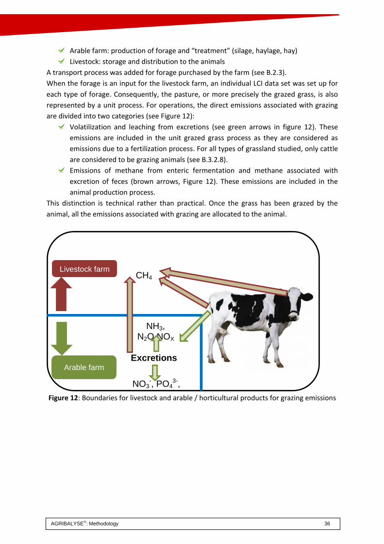
When the forage is an input for the livestock farm, an individual LCI data set was set up for
each type of forage. Consequently, the pasture, or more precisely the grazed grass, is also
represented by a unit process. For operations, the direct emissions associated with grazing
are divided into two categories (see Figure 12):
Volatilization and leaching from excretions (see green arrows in figure 12). These
emissions are included in the unit grazed grass process as they are considered as
emissions due to a fertilization process. For all types of grassland studied, only cattle
are considered to be grazing animals (see B.3.2.8).
Emissions of methane from enteric fermentation and methane associated with
excretion of feces (brown arrows, Figure 12). These emissions are included in the
animal production process.
This distinction is technical rather than practical. Once the grass has been grazed by the
animal, all the emissions associated with grazing are allocated to the animal.
Figure 12: Boundaries for livestock and arable / horticultural products for grazing emissions
NO3-, PO4
3-, ETM
CH4 Atelier animal
Atelier végétal
NH3, N2O NOX
Excretions
Livestock farm
Arable farm

AGRIBALYSE
®: Methodology 37
A.2.3 Data requirements
A.2.3.1 Time-related representativeness
The reference period is the period represented by the data. As a basic rule, in accordance with the AGRIBALYSE® data collection guide, the data collected covers the years from 2005 to 2009. This period was selected to ensure that the data collected:
Was sufficiently recent at the time it was collected to ensure that the LCI data sets
provided the best representation of current agricultural practices,
Covered several years to prevent any bias arising in the LCI data sets owing to an
exceptional year.
The source data statistics for annual crop growing practices only cover part of this period. The representativeness of this part of the data collected was ensured by adjusting the data according to expert opinion. This also applied to the data sets for fruit, vegetables and shrubs, most of which were based on expert opinion (with specific exceptions such as data relating to pesticide inputs). The data sets for special tropical crops and French crops (roses) were based on specific studies undertaken during the reference period.
A.2.3.2 Geographical and technological representativeness
The spatial representativeness of the data sets is given in the metadata and their name. When a data set is said to be representative at national scale (data set with national scope = “national data set”), this has always been achieved by taking account of the agricultural practices of various production systems. This was done either by entering the data directly into a single data set, indicating the frequency of each production practice (using the “area concerned”), or by averaging several individual data sets. The “national data sets” were, therefore, set up using (Table 4):
statistical data entered directly into the data collection module: sugar beet2, durum
wheat, soft wheat, rapeseed, faba beans, silage maize, grain maize, sunflower,
triticale, standard pork - France.
a typical or average case based on expert opinion or a single study: shrubs, coffee,
clementines, all plant data sets for organic farming (soft wheat, faba beans,
peaches/nectarines, apples, tomatoes, triticale), cider apples, grassland.
an average of products with different production systems: conventional carrots,
alfalfa, malting barley, feed barley, conventional peaches/nectarines, peas,
conventional apples, potatoes (excluding starch), grapes for wine-making, roses, Thai
rice, tomatoes for the fresh market, tomatoes for the fresh market in unheated
greenhouse, French milk, French beef, eggs, poultry, turkeys.
For palm oil fruits, a modular approach as been followed (Bessou et al. 2013). Data
come from one plantation extended on two districts, which is divided into several
plantation « blocks » corresponding to different plantation phases. Climate and soil,
as well as farming practices are considered homogenous in all blocks. Compiling the
blocks enable to have data for each phase of the plantation cycle.
2 Five annual data sets were set up for sugar beet and then averaged.

AGRIBALYSE
®: Methodology 38
Table 4: Overview of the main data sources for the data sets and the approach for setting up the data sets. Note: (1) The carrot LCI data sets (several regional variants: Aquitaine, Lower Normandy and production periods: spring, fall, winter) were based mainly on expert opinion (“X (E)”), whereas the national LCI data set (“X (ND)”) was set up by averaging variants. (cf Appendix B also). (2) The LCI data sets for other annual crops (soft wheat, durum wheat, etc) were based mainly on data from agricultural statistics. The product variants and national data sets were based on directly entered data (“X”).
Data set Approach Main data source
ND =National data set V = Product variant
Ave
rage
1)
Dir
ect
dat
a
en
try2)
Stat
isti
cs
Typ
ical
ca
se
Exp
ert
op
inio
n
Arable and horticultural
Annual crops
Sugar beet, barley, peas potatoes, alfalfa
X (ND) X (V) X
Carrots, triticale X (ND) X (V) X
Organic farming data sets X X X
All others X X
Grassland) X (V) X
Fruit
Apples, peaches, grapevines X (ND) X (V) X
Cider apples X X
Special French crops X (ND) X (E) X
Tomatoes and roses X (ND) X (V) X
Shrubs X X
Special tropical crops
Rice X (ND) X (V) X
Clementines and coffee X X
Livestock
Cow’s milk X (ND) X
Beef X (ND) X
Sheep’s milk X
Lamb X
Goat’s milk X
Poultry X (ND) X
Rabbits X
Fish X (ND) X
Pigs X (V) X 1) Special unit processes were set up for the various standard cases. The national data set is an average of the special unit processes. 2) The various standard cases were averaged directly into one single process indicating the area concerned for each crop production practice. 3) There are no national data sets for grasslands in France as the grassland data sets were set up to meet the needs of livestock production data sets.

AGRIBALYSE
®: Methodology 39
Appendix B gives the various methods used in AGRIBALYSE® for calculating the national data sets.
A.2.3.3 Direct emissions
For direct emissions into the environment, the flows of substances (NO3, active substances in pesticides, etc) were taken into account and not the indicators (AOX, COD, BOD, etc). These flows were calculated using various models (see Chapter B.2.4).
A.2.4 Data quality requirements
A.2.4.1 Individual data quality and overall quality of the LCI data sets
AGRIBALYSE® uses three quality levels: Quality of individual data input
The ecoinvent® 2.0 pedigree matrix (Frischknecht et al, 2007) was used to assess the
quality of data entered directly into the data collection module (eg: quantity of
fertilizer applied, daily quantity of feed mix distributed to animals). This approach
was used to determine the confidence interval for data and define the data quality
uniformly across the various data sets in the database. For efficiency and uniformity,
only the type of the source from which particular data was taken was assessed and
this assessment was then applied to all data taken from this source.
Quality of direct emissions in the field and on the farm (calculated data)
For the direct emissions that were calculated using models (see B.2.4), the
ecoinvent® 2.0 pedigree matrix was applied to the model concerned.
Overall quality of the whole LCI data set
To meet the ILCD requirements, the score for the overall quality of the LCI data sets
was calculated by applying the methods defined in the ILCD Handbook (JRC and IES
2010a).
A.2.4.2 Quality of individual data entered
In accordance with the AGRIBALYSE® data collection guide (Biard et al, 2011a) the various types of data sources were classified as follows (Table 5):
Statistical sources, divided into:
- Well documented statistics accessible to the public,
- Statistics with limited access or scientific literature, accessible to the public
Typical cases, divided into:
- Well documented typical case
- Typical case with little supporting documentation
Expert opinion
Individual case / estimate

AGRIBALYSE
®: Methodology 40
The pedigree-matrix (Table 6) was used as a standard by ecoinvent® (Frischknecht et al, 2007) to describe the variance of data and assess the quality. The values of five indicators are processed using a mathematical formula to give a confidence interval of 95%.
Table 5: Types of data source used in the AGRIBALYSE® program and their “quality score” (lognormal distribution confidence interval) based on the ecoinvent® 2.0 pedigree matrix (Table 6). A low value indicates greater precision.
Type of data source Basic
uncertainty Pedigree matrix
values Quality score
(95% confidence interval)
Well documented statistics accessible to the public
1.05 {1,1,1,1,1} 1.050
Statistics with limited access or scientific literature, accessible to the public
1.05 {2,3,2,2,2} 1.108
Well documented typical case 1.05 {1,2,1,1,1} 1.054
Typical case with little supporting documentation
1.05 {2,3,2,3,2} 1.109
Expert opinion 1.05 {3,3,2,1,2} 1.140
Individual case / estimate 1.05 {4,4,2,1,2} 1.245
Note: The basic uncertainty, which draws a distinction depending on the type of data, was taken from Table 7.2 of the ecoinvent® report (Frischknecht et al, 2007). For most inputs, the basic uncertainty is 1.05. For transport it is 2 and for infrastructure (buildings) it is 3.

Table 6: Pedigree-matrix, based on Frischknecht et al, 2007
Indicator score
Indicator 1 2 3 4 5 (default) Remarks
Reliability Verified data based on measurements
Verified data partly based on
assumptions or non-verified data based on
measurements
Non-verified data partly based
estimates by qualified experts
Estimate by a qualified expert
Estimate by a non-qualified source
Verified means: published in public
environmental reports of companies, official
statistics, etc Unverified means:
personal information by letter, fax or e-mail
Completeness
Representative data from all sites
relevant for the market considered, over an adequate period to even out normal fluctuations
Representative data from >50% of the
sites relevant for the market considered, over an adequate period to even out normal fluctuations
Representative data from only some sites (<<50%) relevant for
the market considered or >50% of sites but from shorter periods
Representative data from only one site
relevant for the market considered or some sites but from
shorter periods
Representativeness unknown or data from
a small number of sites and from shorter
periods
Length of adequate period depends on process/technology
Temporal representativeness
Less than 3 years of difference to the time period of the
data set
Less than 6 years of difference to the time period of the data set
Less than 10 years of difference to the time period of the data set
Less than 15 years of difference to the time period of the data set
Age of data unknown or more than 15 years
of difference to the time period of the
data set
Geographical representativeness
Data from area under study
Average data from larger area in which the area under study
is included
Data from area with similar production
conditions
Data from area with slightly similar
production conditions
Data from unknown or distinctly different area (North America
instead of Middle East, OECD-Europe instead of Russia)
Further technological representativeness
Data from enterprises,
processes and materials under
study
Data from processes and materials under study (i.e. identical
technology) but from different enterprises
Data from processes and materials under
study but from different technology
Data on related processes or
materials
Data on related processes on
laboratory scale or from different technology
Sample size
>100, continuous measurement,
balance of purchased products
>20 > 10, aggregated figure in env. report >=3 unknown
Sample size behind a figure reported in the information source

AGRIBALYSE®: Methodology 42
A.2.4.3 Quality of the models for direct emissions in the field and on the farm (calculated
data)
The quality of the models used was also assessed using the pedigree matrix. The criterion for completeness (Table 6) was adjusted by evaluating the number of major parameters considered in the model in question.
Table 7: Models for calculating direct emissions (see B.2.4 for details) used for the AGRIBALYSE® program and their “quality score” (lognormal distribution confidence interval) based on the ecoinvent® 2.0 pedigree matrix (Table 6)
Type of source Model Basic
uncertainty Pedigree matrix
values Quality score
(95% confidence interval)
Fixing of carbon dioxide by the products (CO2)
ecoinvent® v2 1.2 {2,2,1,2,1} 1.209
Land occupation m2.yr and transformation m2
ecoinvent® v2 1.2 {2,2,2,1,1} 1.212
Emissions of ammonia (NH3) EMEP/EEA 2009
Tier 2 1.2 {2,3,2,2,1} 1.218
Nitrogen excreted by the animals
CORPEN 1.2 {2,2,3,3,1} 1.238
Emissions of methane (CH4) IPCC 2006b
Tier 2 1.2 {2,2,3,3,1} 1.238
Emissions of carbon dioxide (CO2) from liming
IPCC 2006b Tier 1
1.2 {2,3,3,4,1} 1.249
Emissions of active substances from pesticides
ecoinvent® v2 1.2 {4,5,1,3,1} 1.372
Emissions of nitric oxide (NO) EMEP/EEA 2009
Tier 1 1.4 {2,4,2,2,1} 1.425
Emissions of dinitrogen oxide (N2O)
IPCC 2006b Tier 1
1.4 {2,4,3,4,1} 1.446
Emissions of nitrate (NO3-) –
modified Comifer grill Tailleur et al, 2012 1.5 {2,3,1,1,1} 1.509
Allocation of P, K and Norg This report 1.5 {2,3,1,1,1} 1.509
Emissions of nitrate (NO3-) –
perennial crops SQCB (Faist et al,
2009) 1.5 {2,3,1,5,1} 1.525
Emissions of nitrate (NO3-) –
tropical crops GIEC 1.5 {3,3,1,3,2} 1.855
Emissions of trace metals SALCA‐SM modified 1.5 {2,2,3,4,1} 1.526
Emissions of phosphorus and phosphate (P, PO4
3-) SALCA-P 1.5 {2,3,3,4,1} 1.530
Emissions of nitrate (NO3-) –
soilless crops This report 1.5 {4,3,1,1,1} 1.564
Land use change (CO2) This report 1.8 {4,3,2,1,1} 1.855
Note: The basic uncertainty, which varies depending on the type of data, was taken from Table 7.2 of the ecoinvent® report (Frischknecht et al, 2007).

AGRIBALYSE®: Methodology 43
A.2.4.4 Overall quality of the LCI data sets in accordance with ILCD
To comply with ILCD requirements, the overall ILCD quality score for the data sets was calculated according to the following six criteria:
Technological representativeness (TeR)
Geographical representativeness (GR)
Time-related representativeness (TiR)
Completeness (C)
Precision / uncertainty (P)
Methodological appropriateness and consistency (M)
These six criteria were evaluated for all the data in a data set, assessing the extent to which the data set met the requirements (on a scale of 1 to 5, 0 for not applicable). The final score was calculated in accordance with the ILCD recommendations. A data set was considered to be “High quality” if the score is ≤ 1.6, “Basic quality” for a score >1.6 to ≤3 and “Data estimate” for a score of >3 to ≤4. As the scales proposed by the ILCD were very generic, to ensure consistent evaluation, the scores for the criterion to be evaluated were specified as follows:
Technological representativeness (TeR): The various agricultural practices considered in the inventory are representative of the total number of production systems used to complete the production considered (considering their distribution / importance). 1 = Very good: nearly all the possible production systems are included in the data set 2 = Good: most of the production systems are considered 3 = Satisfactory: it is not certain that most of the productions systems are considered 4 = Not very satisfactory: Only a few production systems are considered 5 = Unsatisfactory: the data set is based on only one production system
Geographical representativeness (GR): The distribution of production regions for the crop considered in a data set was evaluated, based on the area cultivated (ha), the number of departments covered, or the quantity produced, depending on the data available. 1 = (very good): ≥95% 2 = (good): ≥85% and <95% 3 = (satisfactory/acceptable): ≥75% and <85% 4 = (not very satisfactory): ≥50% and <75% 5 = (unsatisfactory): <50%
Time-related representativeness (TiR): The extent to which the reference period (2005 to 2009) was representative was assessed as: 1 = Very good: data for all five years in the reference period 2 = Good: data for at least three years in the reference period with little change/variation in the production systems 3 = Satisfactory: data on at least two years in the reference period with little change/variation in the production systems

AGRIBALYSE®: Methodology 44
4 = Not very satisfactory: data on two or three years in the reference period but with major changes in the production systems which are not included 5 = Unsatisfactory: data on only one year in the reference period
Completeness (C): this criterion is used to evaluate the flows taken account of in the data set with respect to those given in the data collection guide (GDC). 1 = Very good: all the flows in the data collection guide and major inputs are included 2 = Good: several inputs are not considered but they are not of great importance 3 = Average: some major inputs are not considered 4 = Poor: several major inputs are not considered 5 = Very poor: many major inputs are not considered
Default scores (identical for all data sets) were used for Precision and Methodological appropriateness and consistency.
Precision / uncertainty (P)= 3: “acceptable”, given that the precision of the data was
assessed using the pedigree-matrix and all AGRIBALYSE® data sets are subject to
natural processes resulting in a certain variance.
Methodological appropriateness and consistency (M)= 2: “good”, given that the
calculation models, the system boundaries and the modeling were selected to suit
the aims of the study.
A.2.5 Type of critical review – Quality control
A critical review as defined in ISO 14040/14044 (ISO, 2006a and ISO, 2006b) for situation ILCD-A (see A.1.3) was carried out for the AGRIBALYSE® program. This review concentrated on quality control.
Production system data entered into the data collection module The direct emissions calculation models LCI and LCIA results
Quality control was carried out in three phases:
1. Internal verification: For the AGRIBALYSE® program the data for the LCI data sets and
LCIAs was collected and calculated by different people: “authors” (see metadata:
“author”) and “data generators”. The data collected by the “authors” was verified by
the “data generators”(Colomb et al, 2013).
2. Quality control of the data describing the production systems for the French
agricultural production processes carried out where possible by experts from
organizations external to the project.
3. Quality control of the results of the LCI and LCIA and of the direct emissions
calculation models, carried out by the Technical Institutes.
Phases 2 and 3 each ended with a working seminar.

AGRIBALYSE®: Methodology 45
A.2.5.1 Quality control of French production system data
a) The experts
An independent expert was appointed for each review of a group of similar agricultural production processes (eg: set of oleaginous crop production processes). Experts approached The experts who were selected belonged mainly to an organization external to the AGRIBALYSE® program (Table 8). In several cases, it was not possible to find experts in organizations other than those involved in the program. However, AGRIBALYSE® made every effort to check that they were not involved with setting up the data sets. For tropical products, the control procedure was simplified with only internal control within CIRAD. Table 8: Organizations to which the experts who checked the quality of the production system data belonged
Organization to which experts belonged
Agrial Farming cooperative
Chambre Régionale d’Agriculture de Bretagne
Agricultural development
Agrocampus Ouest Educational and research institute
Chambre Régionale d’Agriculture des Pays-de-la-Loire
Agricultural development
Agro-Pithiviers Farming cooperative
ESA Angers Education
Agro-Transfert Picardie
Technology transfer IDELE Technical Institute
Axereal Farming cooperative
INRA Research Institute
Biomar Feed manufacturer InVivo Farming cooperative
Chambre d’Agriculture 44
Agricultural development
IRBAB (Institut Royal Belge pour l’Amélioration de la Betterave)
Technical Institute
Chambre d’Agriculture 53
Agricultural development
ITAB Technical Institute
Chambre d’Agriculture 66
Agricultural development
Lycée de Guérande Education
Coop de France Farming cooperative
SILEBAN Regional experimental station
The main criteria for selecting the experts were their independence, their qualifications and their experience.

AGRIBALYSE®: Methodology 46
Procedure for selecting the experts
Selection of organizations for quality control by the AGRIBALYSE® Strategic Committee
Proposal of experts by the Technical Institutes Proposal of experts by the organizations selected for quality control Selection of the experts by the Strategic Committee from the proposals made by the
organizations and Technical Institutes on the basis of the following criteria.
Expert selection criteria The minimum criteria taken into account for selecting the experts were:
Technical knowledge of the systems studied at regional level but above all at national level
Independence with respect to AGRIBALYSE® Availability
b) Documentation
The following documents were produced for the quality control phase. Specification for the experts This was a technical document (Appendix C) to simplify the quality control work of the experts by detailing the data to be reviewed and the review process. This document defined the scope of quality control required. It also defined that, when modifications were required, the quality of the modifications should be subject to a second review. Review forms Review forms were sent to the experts to provide uniform results. These forms were specific to each livestock or arable / horticultural production system and are attached at Appendix C. One form was filled in for each data set checked. These forms have:
A pre-printed section: to ensure that the experts check critical points A blank section: for comments by the expert on the general quality of the process
Confidentiality The quality of the production system data was checked with the proviso that the data sent to the experts should remain confidential and be used only for quality control. Experts confirmed that data would be kept confidential by signing a confidentiality agreement before the data was sent.
c) Scope of the quality control procedure
The experts were requested to check the data describing the production systems. They were not asked to assess the methodological decisions made for the project (system boundaries, functional units, allocation, etc). Details of the data to be reviewed were defined in a specification. The experts were also asked to comment on any omissions or incoherence in the descriptions of the production systems.

AGRIBALYSE®: Methodology 47
A.2.5.2 Quality control of LCI and LCIA results
The quality of the LCA/LCIA data calculated by Agroscope and INRA was checked by the Technical Institutes involved in the AGRIBALYSE® program according to a common procedure.
a) The experts
The data was checked by the Technical Institutes involved in the AGRIBALYSE® program.
b) Documentation
To carry out the quality control, files summarizing the results of the LCIA were drawn up and exchanged for each data set. These files also contained technical data (eg. results of nutritional components, results of fuel consumption, etc.) to check that the data entered into the data sets was processed correctly. The Technical Institutes returned the results of their reviews using a specifically designed form.
c) Scope of the quality control
The quality control considered the relevance of the results of the LCIA and LCA and the parameters for the direct emissions calculation models. This was done in several stages: verifying the calculations, comparing the internal references and the results in the works cited in the bibliography. The procedure ended by pooling the comments at a working seminar and by the Technical Institutes drawing up an evaluation report. This report is included in the report “AGRIBALYSE®: Assessment and lessons for the future” (Colomb et al, 2013).
A.2.6 Type and format of the report required for the study
ISO 14044 (ISO, 2006b) and the ILCD Handbook (JRC and IES, 2010a) give recommendations for the types of deliverables expected. In accordance with these recommendations, AGRIBALYSE® results were produced in the following formats:
A report on the methodology setting out the bases for the study (this report)
For each product, the results are given as:
impact indicator values (LCIA)
LCI flow data sets
The report “AGRIBALYSE®: Assessment and lessons for the future” (Colomb et al, 2013), describing how the program was carried out and the main results of the program, including two notes on the quality control of the LCI data sets and the results as well as an exploratory sensitivity analysis for sugar beet and pork.
Incorporating the data sets into the IMPACTS® database requires the results to be in terms of flow (LCI) rather than impact indicators, as the impacts are calculated automatically from the flows and the characterization factors selected by the ADEME-AFNOR platform on the basis of JRC recommendations. However, it proved necessary to have the LCIA results in order to be able to analyze the results for each product in subsequent projects.

AGRIBALYSE®: Methodology 48
To simplify the distribution of the results, AGRIBALYSE® also provided the following documents:
A summary for each product to give a rapid overview of the main results without
requiring LCA software
A database meeting ILCD requirements (for situation ILCD-A, see A.1.3), in the form
of unit processes, containing the data sets produced during the program

AGRIBALYSE®: Methodology 49
Part B – LCI data sets
B.1 Data collection procedures and systems used for AGRIBALYSE®
AGRIBALYSE® was designed to ensure that the processes selected could be compared. The following procedures and systems were used to produce the LCI data sets using a consistent methodology to ensure that the data sets could be compared so far as possible.
Common rules were set out for defining systems and data collection procedures and a special data collection module was developed. These rules are published in the Data Collection Guide (GDC, see B.2.1)
A data collection module was used to input the data for the various livestock and arable / horticultural products in a uniform format (see B.2.1)
A set of EXCEL spreadsheets was used for calculating direct emissions and systematic processing of the input data in ecospold format (calculation chain, see B.2.1)
Simapro® + ecoinvent®: Most of the upstream and indirect flows were calculated using Simapro® and the ecoinvent® database ® v3.2, cutt off version (called « allocation recyclesd content » in SimaPro).
B.2 Data collection
B.2.1 Data collection
B.2.1.1 Data collection module
The data collection module used Excel and VBA (Visual Basic for Applications) for entering the raw data in a standardized format. The data collection module was based on a form developed and used for a CASDAR project (CASDAR AAP 7-175 “Improving economic and environmental performance of pea, rapeseed and wheat production systems”). As this form only allowed data to be entered for production systems for annual French crops, it had to be modified to meet the requirements of the AGRIBALYSE® program:
Design and incorporation of input spreadsheets for the various livestock and special products (greenhouse crops, permanent crop systems)
Minimizing the diversity of inputs by defining default values (accessible using dropdown menus) to simplify data collection and ensure that descriptions were uniform
Design to allow lists of inputs / dropdown menus to be extended Documentation of the production systems as required by the ILCD Handbook (JRC
and IES, 2010a) Inclusion of the evaluation of the quality of each data item depending on its source Possibility of comparing the data sets/production systems entered
Two documents were produced describing how to use the data collection module: the Data Collection Guide (Biard et al, 2011a) and the Data Collection Module Manual (Biard et al, 2011b).

AGRIBALYSE®: Methodology 50
B.2.1.2 Data Collection Guide
The Data Collection Guide (Biard et al, 2011a) gave practical help during the data collection phase for the AGRIBALYSE® program. It ensured that all production system data was consistent. The Data Collection Guide is both a guide for data collection (Part A) and a guide to good practices for modeling the production systems covered (Part B). The rules set out in the guide were implemented in the data collection module.
B.2.1.3 Data collection module manual
This manual describes how to use the data collection module. It describes the various input fields and how the data collection module operates.
B.2.2 Input data categories
B.2.2.1 Inputs
The collection of all the data, i.e. the entry of all the information required to take account of the components on the system (see chapter A.2.2), was undertaken by the Technical Institutes, using the data collection module.
a) Arable and horticultural products
The following information was collected for each input: The name of the specific input (eg. ammonium nitrate, rabbit liquid manure or
metolachlor). The names of items were selected from a predefined list which could be extended if necessary on condition that a definition was given for each new item.
The quantity applied / consumed (specifying the units) The data source The percentage of area concerned, to take account of different practices in certain
production systems (eg: 30% no till; 70% sowing with drill) The date of application and the minimum and maximum values of the data. This was
optional, as the information was not strictly necessary for the LCI. Optional comments

AGRIBALYSE®: Methodology 51
Table 9 lists additional information require for each input category.
Table 9: Additional data collected for each input category
Input category Additional data collected Products concerned
Sowing seed Proportion of farm seed sown Annual crops
Fertilizer (organic/mineral) Number of applications All
Pesticides Number of applications All
Agricultural process - Tillage - Sowing seed - Fertilization - Applying pesticides - Tending crops - Harvest
Number of applications All
- Irrigation Amounts of water applied, source of energy used and amount of energy consumed
All
Buildings Area Special French crops (greenhouses)
Other inputs Purpose All
The data was entered using predefined lists. When a new item (fertilizer, active substance, process) was introduced, the following information was entered to build a specific LCI data set or modify an existing data set:
New fertilizer: name, units, composition (total N, plant available N, P2O5), source. New agricultural process: name of process, description, units, machinery required
(traction and no more than two machines), operation time, consumption and type of power, source.
New machine: name of the machine, description, lifetime, weight of the machine, footprint, source.
b) Livestock production
Two types of data were collected for livestock production data sets Data describing the class of animal (eg: number of animals at start, age and weight of
animal on acquisition and disposal, mortality, etc.) Data on animal feed. Data was entered in two stages. The first stage defined the
feed mix and the second stage defined the annual ration. In the first stage, the raw materials and their proportions in the feed mix were defined. In the second stage, the feed mixes and/or the basic fodder (raw materials consumed directly by the animals including forage and grazed grass) were defined to give a precise record of the ration distributed to the animals.
B.2.2.2 Direct emissions
The flows of potentially polluting substances directly associated with the livestock and arable/horticultural production processes (direct emissions) are not entered but calculated by the inventory data processing system (IDPS), see chapter B.2.4. The data and parameters required for calculating direct emissions are described in the datasheets (Appendix D).

AGRIBALYSE®: Methodology 52
B.3 Calculating the LCI data sets
B.3.1 Data processing applications
The AGRIBALYSE® data sets were drawn up using a set of EXCEL spreadsheets, called Inventory data processing system (IDPS), to ensure that data was processed consistently and could be compared. The IDPS used the data from the data collection module and converted it into a “unit process” in ecospold format, adding the direct emissions and transport for the inputs. This format makes the data set compatible with LCA applications. The IDPS had two main sections:
Software implementing the models for calculating the direct emissions: 15 models
were drawn up or modified for calculating the direct emissions (Table 10).
Table 10: Models for calculating direct emissions (see chapter B.2.4)
Substance emitted Calculation procedure
CH4 EXCEL spreadsheet, developed by AGRIBALYSE®
CO2 biogenic EXCEL spreadsheet, developed by AGRIBALYSE®
CO2 due to land use change Method developed by AGRIBALYSE®
CO2 due to liming EXCEL spreadsheet, developed by AGRIBALYSE®
ETM Modified SALCA spreadsheet
N2O EXCEL spreadsheet, developed by AGRIBALYSE®
NH3 EXCEL spreadsheet, developed by AGRIBALYSE®
NO3- EXCEL spreadsheet, developed by AGRIBALYSE®
NO EXCEL spreadsheet, developed by AGRIBALYSE®
Land occupation and transformation EXCEL spreadsheet, developed by AGRIBALYSE®
P, P2O4 Modified SALCA spreadsheet
NPK reallocated EXCEL spreadsheet, developed by AGRIBALYSE®
Active substances (pesticides) EXCEL spreadsheet, developed by AGRIBALYSE®
Substances emitted by farmed fish (Ntotal, Ptotal, TSS/COD)
EXCEL spreadsheet, developed by AGRIBALYSE®
Intermediate spreadsheet
Calculation of nitrogen excretions from animals EXCEL spreadsheet, developed by AGRIBALYSE®
Calculation of soil loss EXCEL spreadsheet, developed by AGRIBALYSE®
Data conversion module: This module took the results of the direct emissions
calculation procedures and the data on inputs from the data collection module and
converted the information into a unit process in ecospold format. It was based on the
SALCA system developed by Agroscope.

AGRIBALYSE®: Methodology 53
Figure 13 shows how these modules operate and interact.
Figure 13: Components in the Inventory Data Processing System Each component of the inventory data processing system was designed or specifically modified to meet the requirements of the AGRIBALYSE® program. Information about accessing the applications can be found in the report “AGRIBALYSE®: Assessment and lessons for the future” (Colomb et al, 2013).
B.3.2 Relating data to the functional units
In several cases, data was collected for the data collection unit which is different from the functional unit (in general, the data collection unit for arable / horticultural data sets is the hectare and that for livestock data sets is the herd). Data sets were related to the functional units using a conversion factor, based on the reference flow also defined during data collection.
B.3.3 Calculating the LCI data sets of inputs for agricultural production
AGRIBALYSE® distinguished three types of input for agricultural data sets: 1. Agricultural inputs (from France or elsewhere) – for example: forage barley, seed,
etc. These inputs were taken from the agricultural sector and their data sets were
developed by the AGRIBALYSE® program.
2. Non agricultural inputs specific to agriculture – for example: tractor, pesticides,
fertilizers, etc.
Processing by the IDPS
1. Allocate primary data data set 2. Check units 3. Calculate amount consumed 4. Calculate transport 5. Allocate
Inventory Data Processing System
(IDPS)
INPUT DCM XY
15 Models
X-Exchange Product XY
IF IDPS/Mod. IF Mod./IDPS
IF DCM/IDPS
IF = interface

AGRIBALYSE®: Methodology 54
3. Non agricultural inputs not specific to agriculture – for example: electricity, diesel,
steel for fencing, tires for tractors. These inputs were produced outside the
agricultural sector and are used by all economic sectors.
The basic principle of the AGRIBALYSE® program for the LCI data sets/ LCA for type (2) and (3) inputs was that priority should be given to data in the IMPACTS® database or, if not in this database, in other recognized databases. However, few data sets meeting the requirements for coherence with the AGRIBALYSE® methodology (boundaries, flows) and representativeness were found. For this reason, most of the data sets used came from the ecoinvent® database. However, as the ecoinvent® data sets were not always applicable to France, type (2) inputs were modified, where possible, using existing data sets (see following chapters). The correspondence “inputs <-> existing LCI data sets” is given in Appendix G. When necessary, data sets for type (2) inputs were set up on the basis of existing data sets and modified to suit conditions in France. For example:
Machines: the size of the machines and operation time were adjusted to conditions
in France and the tropical production systems studied.
Livestock buildings: the source data came mainly from the CASDAR project “Eco-construction and livestock buildings” (IE et al, 2009). The units used were the annual area used in m2.yr or a space used for one year.
Fish farm buildings: the data sets used for fish farm infrastructure was taken from the databases of UMR-SAS, INRA, Rennes.
Plant production buildings: data sets based on data from French manufacturers were used for greenhouses (glass greenhouses, air-inflated double polyethylene film greenhouses and polytunnels), (Boulard et al, 2011).
The procedures implemented for building LCI data sets when existing data sets were not included in existing databases are described below.
B.3.3.1 Sowing seeds and growing plants
The following approaches were used to build seed and plant data sets: 1. Extrapolation by applying a factor to the data set for the crop grown for sale. The
“seed” data set flows (resources required and emissions) were calculated by
multiplying the “crop” data set by an extrapolation factor. Data on ten crops3 was
available from GESTIM (Gac et al, 2010) but the data sets were drawn up to study the
impacts of primary energy consumption and climate change. Certain inputs and flows
contributing to other impacts were not included or not sufficiently detailed. The
quantities for the inputs and missing flows were obtained by multiplying the
quantities obtained for the data set for the crop grown by an extrapolation factor.
This factor was the ratio between the consumption of primary energy obtained from
3 Durum wheat, soft wheat, sugar beet, rapeseed, maize, barley, peas, potatoes, triticale, sunflowers.

AGRIBALYSE®: Methodology 55
GESTIM for seed production and that for the product listed in the data collected for
the AGRIBALYSE® program (see Appendix D, Datasheet 15).
2. Building a separate data set
3. If the information required was not present: substitution of the data set for the crop
grown or use of an existing LCI data set.
The extrapolation approach was applied for ten annual crops: sugar beet, durum wheat, soft wheat, rapeseed, maize (grain and silage), barley (brewing and forage), peas, potatoes, sunflowers and triticale. For « similar crops », the most common se bought was used : all wheats have a seed extrapolated from the « average wheat », all maizes have a seed from « grain maize » and all barleys have a seed from « spring barley » (Table 140). Approach 2 was also applied to carrots and tomatoes using expert opinion. Approach 3 was used for the other crops: for faba beans and organic annual crops (soft wheat, triticale), seed sowing was taken into account by substituting the data set for the final product. The ecoinvent® data sets were used for grassland and alfalfa. For orchards, grapevines, coffee and clementines, an equivalent area was calculated by working out the number of hectares of cuttings and grafts required to plant one hectare of orchard/enclosed area. The orchard/vineyard in full production data set was taken as a substitute.
B.3.3.2 Average fertilizer data sets
Three “average N/P/K fertilizer” data sets (average mineral fertilizer, as N/P/K, at regional storehouse, FR) were set up based on the average mineral fertilizer consumption from 2005 to 2009 in France for which an LCI data set was available (Appendix I). The UNIFA database was used for this, taking the data for deliveries of fertilizer for the years 2004/2005 to 2008/2009 (UNIFA, 2009). The non-specified 2 and 3 compound fertilizers categories (PK, NP, NK, NPK) were allocated to ecoinvent® data sets using more detailed analyses from GESTIM (Gac et al, 2010). Organo-mineral fertilizers were allocated to the other fertilizers depending on their N/P/K content. The transport distances from the place of production to the point of sale were also based on GESTIM analyses (Gac et al, 2010). Details are given in Appendix I.
For farm manure (manure, liquid manure) “phantom LCI data sets” with no environmental impact were set up to ensure that the direct emissions related to their application were calculated correctly and to make it easier to check the data sets.
B.3.3.3 Machine data sets
New data sets were calculated based on the information entered in the data collection module, by parameterizing the six machine data sets available in the ecoinvent® database. The machine datasets include the flows related to:
Production
Repair
Maintenance of tires and engines (if appropriate)
End of life (waste management)

AGRIBALYSE®: Methodology 56
Table 11 summarizes the parameters for the various components of these data sets. The flows related to maintenance are required only for powered machines (oil and filters) and wheeled machines (tires). Table 11: Parameters for machine data sets using the available ecoinvent® data sets
Data set component Parameter required
Trac
tors
Har
vest
ers
Trai
lers
Slu
rry
tan
kers
Agr
icu
ltu
ral
mac
hin
ery,
ge
ner
al
Agr
icu
ltu
ral
mac
hin
ery,
ti
llage
Production Weight
yes yes yes yes yes yes Waste management yes yes yes yes yes yes Repair Weight and lifetime
(repair factor)
yes yes yes yes yes yes Waste management yes yes yes yes yes yes Maintenance (tires) Weight and lifetime of
machine/tire
yes yes yes yes yes no Waste management yes yes yes yes yes no Maintenance (filters, oil) Weight and lifetime of
machine
yes yes no no no no Waste management yes yes no no no no
The 213 machines defined in the data collection module were divided into the following 14 groups4 depending on: i) ecoinvent class of machine (tractors; harvesters; trailers; agricultural machinery, general; agricultural machinery, tillage; slurry tankers) and ii) the lifetime.
1. Tractors, 7,500 h 2. Tractors, 10,000 h 3. Tractors, 12,000 h 4. Harvesters, <5000 h 5. Harvesters, 5,000 – 10,000 h 6. Harvesters, > 10,000 h 7. Trailers <20 t 8. Trailers, >20 t 9. Slurry tankers, 5000 l, 10. Agricultural machinery, general, <2,500 h 11. Agricultural machinery, general, 2,500 -5,000 h 12. Agricultural machinery, general, >5,000 h 13. Agricultural machinery, tillage 14. Machine with electric motor
The functional unit for machine data sets is always “1 kg machine for the total lifetime”. Details are given in Appendix J.
B.3.3.4 Agricultural process data sets
An agricultural process covers the flows related to the use of the infrastructure for tilling, maintenance and harvesting:
4 Four standard ecoinvent® data sets are used for lorries (lorry 16t/RER/I U, lorry 40t/RER/I U), vans (van
<3.5t/RER/I U) and helicopters (Helicopter/GLO/I U).

AGRIBALYSE®: Methodology 57
Production, maintenance and end of life of the machines used for the process (eg. a
tractor and a plow with five blades for the “plowing” process).
All the inputs and outputs required for the operation of the infrastructure, i.e. energy
(diesel, electricity) and emissions from burning fuel. However, variable products,
distributed or applied by the processes, such as the fertilizers or active substances,
are not included. These inputs were specified separately.
The storage facilities for machinery: shed or open air area.
New data sets were set up based on the information entered in the data collection module (operation time, diesel fuel consumption etc.). The 258 agricultural processes specified initially in the data collection module were harmonized and grouped into 139 final processes, in collaboration with the technical Institutes (Appendix K). For coherence with ecoinvent®, an “agricultural process” data set covered the following elements:
The requirements for one or more machines
The power requirement (fuel/electricity, etc.)
Emissions related to the use of the fuel (if appropriate)
Wear on the tires (if appropriate)
The requirement for a garage to house tractors and automotive machines or the area
required for attachments and trailers (open air storage).
The functional unit for agricultural processes was “one hour of work”, which is different
from the ecoinvent® convention where in most cases the functional unit is “one hectare”.
This convention is more flexible and makes it possible to take account of different times
required (h/ha) for the same process (for example for tilling different types of soil). The
machine requirement for one hour of process is calculated by dividing its weight by its
lifetime (because the functional unit for the machine LCI data set is kg machine for the
whole lifetime).
machine theof Li fetime
machine theof Weight trequiremen Machine

AGRIBALYSE®: Methodology 58
B.3.3.5 Active substances
The active substances used in pesticides were assigned to existing LCI data sets. Based on the pesticide index (ACTA, 2005 and ACTA, 2009), an active substance was assigned to an existing data set (eg: “cyclic N-compounds, at regional storehouse/kg/RER”, “Pyridine-compounds, at regional storehouse/kg/RER”) using its chemical family. When this was not possible, it was assigned to a more generic data set (“pesticides unspecified, RER at regional storehouse”, “herbicides unspecified …” etc.).
Examples Fluazinam chemical family: pyridinamine Pyridine compounds, at regional storehouse RER Flurtamone chemical family: furanone Pesticides unspecified, at regional storehouse, RER
The assignment of all active substances covered in the AGRIBALYSE® program is given in Appendix G.
B.3.3.6 Greenhouse LCI data sets
Existing data sets were used and modified for greenhouses (glass greenhouses, air-inflated double polyethylene film greenhouses and polytunnels) (Boulard et al, 2011). These had to be modified for reasons of coherence, uniformity and consistency. In the original data sets, several inputs were linked to non ecoinvent® data sets. For example, for steel, the LCI data set “X12Cr13 (DIN 1.4005, AISI 416)” in the IdeMAT database (IdeMAT, 2001) was used whereas in AGRIBALYSE® the steel considered was always “steel, low-alloyed, at plant/kg/RER”. The modified greenhouse data sets are available in the AGRIBALYSE® database.
B.3.3.7 Livestock building data sets
The livestock building data sets used: Were taken from the internal databases of UMR SAS (INRA, Rennes) for
infrastructure related to aquaculture
Were built using data from the CASDAR project “Eco-construction of livestock
buildings” (IDELE et al, 2009)
B.3.3.8 Animal feed data sets
Most of the LCI data sets for elementary feed, grazing and forage were produced for the AGRIBALYSE® program, adding transport if necessary. The feed mixes contain many raw feed materials (RM) for which LCI data sets were not produced within the program and so the RM data sets used for the formulation (fabrication) of commercially available food concentrates came from:
LCI data sets for products from the arable sector of AGRIBALYSE®: soft wheat, organic soft wheat, faba beans, organic faba beans, rapeseed, sunflower seed, cut grass (silage or haylage), grazed grass, alfalfa for dehydration, maize silage, maize grain, forage barley, peas, sugar beet, triticale and organic triticale.

AGRIBALYSE®: Methodology 59
LCI data sets from internal databases from the UMR SAS (INRA, Rennes) that were processed by the AGRIBALYSE® inventory data processing system. The production system data contained in these databases was entered into the data collection module and the LCI data sets were generated by the AGRIBALYSE® inventory data processing system (IDPS). These data sets were for forage, cereals and oil and protein crops.
LCI data sets from internal databases from the UMR SAS (INRA, Rennes) that were used without being processed by the IDPS. These are products other than raw plant materials that could have been processed by the IDPS, or products that had been subject of specific studies (eg: soybean from Brazil).
LCI data sets from commercial databases (ecoinvent®, etc). These were sometimes modified to comply with the project requirements.
The data sets for feed mixes, in the system data set format, were made available for use in AGRIBALYSE®. The procedure for carrying out these processes is described in Appendix L. Note on calculating grazed grass data sets. For the AGRIBALYSE® program, grassland and grazed grass were treated in the same way as other forages, which meant that a special data set was set up (see A.2.2.4b). The data collected for the AGRIBALYSE® program strictly only covers grazing for cattle. The grazed grass data sets were also used without modification for sheep and goats considering that: a) in France, most ruminants are cattle b) the accounting (expressed in large cattle units) is comparable, which means that the
overall yields and excretion can be compared c) for calculating the direct emissions linked to excretions, the composition of cattle
manure was used. The losses at harvest were taken into account in the data sets for grass that was grazed or used for hay, silage or haylage. To calculate the yield, the losses on collection, storage and consumption of forage by the animals were subtracted (Appendix L, §3).
B.3.4 Transport of inputs
Transport of inputs from the point of purchase to the farm was taken into account using transport models. A transport model brought together the information on the means of transport used and the distances travelled and was applied to groups of inputs. The following types of input were considered:
Fertilizers (mineral and organic) Pesticides Other inputs Raw materials for feed (note: when the forage and raw materials were produced on
the farm, transport was not considered).
In these models, the journey from the “point of purchase” (storage / distribution site) to the “farm” may cover the two components shown in Table 12.

AGRIBALYSE®: Methodology 60
For the weight transported, the gross weight was taken into account. In accordance with ecoinvent® (Nemecek and Kägi, 2007), an average content of active substances in pesticides of 50% was used to estimate the weight of the pesticide based on the amount of active substance applied. Table 12: Assumptions for transport of inputs
Type of input Transport from point of
purchase outside France to point of purchase in France
Transport from point of purchase in France to the
farm
Inputs produced on the farm No No
Inputs produced in France (FR type data set)
No Yes: 15 km with tractor and
trailer
Fertilizers, raw materials for imported feed
Yes (see details in Table 13)
Other imported inputs (RER type data set)
Yes based on Ecoinvent “v3 market processes”
For AGRIBALYSE® data sets for France, the distance between the point of purchase and the farm considered was 15 km with tractor with trailer/tank. For organic fertilizers which come from the farm itself or a nearby farm, 10 km transport with tractor and trailer was assumed. In addition, on farm transport (farm-field) is included in “agricultural process” LCIs data sets, also amounting to about 10 km (Appendix K). As no data was available, the same assumptions were applied for tropical crops: clementines, coffee and rice.
For imported inputs, default assumptions from ecoinvent have been used through “market processes”, except for mineral fertilizers and feeds where specific transportation data could be defined based on GESTIM (Gac et al, 2010) (Table 13). For animal feed:
Transport from the place of production/storage of the raw material to the feed fabrication plant
Transport of the feed from the feed fabrication plant to the farm For feed produced on the farm, only the transport of raw materials from their place of production/storage to the farm was considered. An average transport distance in France, depending on the means of transport, was calculated according to Nguyen et al (2012). For raw materials coming from abroad, the transport distance proposed by GESTIM (Gac et al, 2010) was used. Table 13: AGRIBALYSE® transport models (TM) used for animal feed
ecoinvent® process Place of fabrication of raw
material Fabrication plant Fabrication plant
Farm Transport, lorry >32t, EURO3/RER U 110 kma + GESTIMb assumption 130 kmb Transport, freight, rail/RER U 390 kma + GESTIMb assumption - Transport, transoceanic freight ship/OCE U GESTIMb assumption - a transport distance in France calculated according to Nguyen et al (2012).
b transport distance according to Gac et al (2010).

AGRIBALYSE®: Methodology 61
B.3.5 Calculation models for the consumption of resources and direct emissions
from polluting substances
B.3.5.1 General principles and overview of the models used
In AGRIBALYSE®, direct emissions were defined as flows of potentially polluting substances into the environment, directly associated with livestock and arable/horticultural production, on their production site. This was, however, extended to cover the consumption of resources required for the production processes (water consumption, land occupation, etc). As recommended in the ILCD Handbook (JRC and IES, 2010a) and ISO standards (2006a and 2006b), so far as possible, only the flows of elementary substances were calculated. COD (chemical oxygen demand) indicators and AOX (adsorbable organic halogens) were not considered. Indirect emissions, flows of potentially pollution substances into the environment associated with the production of inputs used on the production site, were not modeled in AGRIBALYSE®. These indirect emissions are part of the generic data in existing databases (ecoinvent®, etc). AGRIBALYSE® was based on the recommendations in international standards to rationalize the choice of models used for the program. According to the recommendations of IPCC (2006a) and EMEP/EEA (2009), the models used should make it possible to produce an estimate that is as precise and correct as possible. Models that introduced a systematic bias could not be used. Several criteria were taken into account when selecting models for calculating direct emissions and consumption of resources:
The scientific validity: AGRIBALYSE® aimed to be recognized internationally and so
the methods used had to be recognized scientifically and be subject of international
consensus.
The scope of validity: as AGRIBALYSE® set up data sets mainly for French agricultural
products, the models used must, at least, be applicable to conditions in France.
Technical feasibility: AGRIBALYSE® focuses on using models that are easy to apply in
particular concerning the quantity of data required to use the calculation models.
The granularity of the models selected must be compatible with the input data
collected.
The models for calculating direct emissions and the consumption of resources for tropical
products were selected on the same principles, the scope of validity being adapted to each
product considered.
This section of the report presents the main requirements for each substance emitted, the models identified in the literature which could possibly be used in AGRIBALYSE® and the models and the sources of emissions finally selected. The parameters for all the models are described in Appendices D, E and F.

AGRIBALYSE®: Methodology 62
a) Substances / direct emissions considered
Agricultural production operations generate direct emissions and consume resources. Table 14 presents the emissions and resources consumed and the sources of the emissions considered and the models selected. The choice of model does not indicate that a given model is considered to be scientifically better than the other models. The models were selected to meet the requirements and aims of the AGRIBALYSE® program.

AGRIBALYSE®: Methodology 63
Table 14: Substances emitted/resources consumed, sources of emissions and models used in AGRIBALYSE®
Substance emitted /
Resource consumed
Source of emissions /
consumer of resource Model used
Ammonia (NH3)
Animal excretion (building/ storage)
- calculation of nitrogen excreted CORPEN 2006, 2003, 2001, 1999a and 1999b
- emission factors EMEP/EEA 2009 Tier 2
Organic fertilizers and excretion on grassland EMEP/EEA 2009 Tier 2
Mineral fertilizers EMEP/CORINAIR 2006 Tier 2
Thai rice Yan et al, 2003b
Carbon dioxide (CO2) Absorption by the plants ecoinvent® v2 (Nemecek and Kägi, 2007)
Addition of lime and urea IPCC 2006b Tier 1
Trace metals (Cd, Cu, Cr, Hg, Ni, Pb, Zn)
Leaching: French crops
SALCA‐SM adapted for France (Freiermuth, 2006 and SOGREAH, 2007)
Runoff: French crops
Accumulation in the soil: French crops
Energy stored by the plants
All arable and horticultural production Higher heating value (HHV) of the product
Combustion gas
CO2 ecoinvent® v2 (Nemecek and Kägi, 2007), using an LCI “combustion of diesel/kerosene” data set
Other air pollutants (metals, VOC, SOX, NOX…)
Methane (CH4)
Animal excretion (building/ storage/grassland/outdoor run)
IPCC 2006b Tier 2
Emissions from enteric fermentation: cattle and sheep
IPCC 2006b Tier 2
Emissions from enteric fermentation: other animals
IPCC 2006b Tier 1
Thai rice IPCC 2006b Tier 2
Nitrate (NO3)
Leaching: annual crops Tailleur et al, 2012
Leaching: special orchard crops, vineyards SQCB (Faist et al, 2009)
Leaching: special soilless crops This report: based on waste water/losses
Leaching: grassland This report
Leaching: tropical crops (except rice) IPCC 2006b Tier 1
Thai rice This report: based on water balance
Livestock production: outdoor runs Basset-Mens et al, 2007
Land occupation All types of production ecoinvent® v2 (Frischknecht et al, 2007)
Nitric oxide (NO)
Livestock and arable/horticultural production
EMEP/EEA 2009 Tier 1
Thai rice IPCC 2006b Tier 2
Phosphorus (P)
Leaching: French crops
SALCA-P (Nemecek and Kägi, 2007 and Prasuhn et al, 2006)
Run-off: French crops
Emissions from grazing and grassland
Tropical crops (except rice)
Special soilless crops This report: based on waste water / losses
Thai rice This report: based on water balance
Pesticides
Application of the product: French crops, clementines, coffee
ecoinvent® v2 (Nemecek et Kägi, 2007)
Application of the product: Thai rice This report
Dinitrogen oxide (N2O) Arable / horticultural production IPCC 2006b Tier 1

AGRIBALYSE®: Methodology 64
Substance emitted /
Resource consumed
Source of emissions /
consumer of resource Model used
Special French crops IPCC 2006b Tier 1
Tropical crops (except rice) IPCC 2006b Tier 1
Thai rice IPCC 2006b Tier 2
Livestock production (buildings and storage) IPCC 2006b Tier 2
Soil lost
French arable / horticultural production in open fields
RUSLE (Foster, 2005)
Soilless production Loss set to 0
Tropical products Loss set to 0
Land transformation All types of production ecoinvent® v2 (Frischknecht et al, 2007)
Phosphorus , nitrogen, total suspended solids (TSS)
Aquaculture Papatryphon et al, 2005
b) Flows not considered
Several flows were not taken into account by AGRIBALYSE® CO2 emissions produced by animal respiration: in accordance with the
recommendations of IPCC (2006b). The CO2 absorbed by the plants during
photosynthesis, and therefore contained in cattle feed, was considered to be
restored to the atmosphere in this form. As this is not a long-term storage process,
this type of emission did not need to be considered.
Carbon sequestration in the wood of permanent crops (grapevines and trees): it
is difficult to evaluate the fate of the wood (storage or short cycle), the amounts of
CO2 involved are low, in accordance with the calculations carried out by CITEPA for
national data sets (CITEPA, 2011).
Changes in biomass and soil carbon stocks after land use change (LUC) in France:
although two methods were developed for taking account of the changes in soil
carbon stocks (Salou et al, 2012: Appendix E), this source / sink of emissions was
not included in the data sets in the database.
Water sampling flows: More precise methods for including the water footprint
(green, blue and gray) in LCI data sets are currently being developed (Appendix F).
The method considered to be the most efficient at the moment is that developed
by Pfister et al (2009). However, it was not considered to be applicable for
AGRIBALYSE®. The direct consumption of water was, therefore, only taken into
account for irrigation, fertigation and drinking and cleaning water.
Gaseous emissions from fish farming were not taken into account as insufficient
data was available for trout and no data was available for the production of sea
bass / sea bream. Data is being collected for these types of emissions.
Only Cd, Cu, Cr, Hg, Ni, Pb and Zn, were included for trace metals, as no reliable
data was available for the other metals .

AGRIBALYSE®: Methodology 65
Particulate emissions from activities on the farm (animal and plant production).
The data currently available in France and Europe was considered to be
insufficient to take satisfactory account of these emissions (Faburé et al, 2011).
Parameters could not be defined for the trace metal and soil loss models for
tropical products as there was a lack of information/data.
Of the various NOx gases only NO was considered for direct flows, owing to the
lack of appropriate models for the other gases.
A detailed description of the parameters for models for calculating NH3 emissions is given in Appendix D – Datasheet 1.
B.3.5.2 Calculation of ammonia emissions (NH3)
a) Challenges and requirements
In agricultural production systems, ammonia is emitted by volatilization of the nitrogen content:
In mineral and organic fertilizers
In excretions from animals while grazing or in buildings
In animal excretions during storage
These emissions depend on the type of fertilizer applied or the type of excretion and on soil, climatic and microbiological conditions.
b) Available models
Several models were found in the literature: CORPEN (2003) and CORPEN (2006)
MELODIE (Chardon et al, 2011)
Gac et al, 2006
STICS (Brisson et al, 1998)
Volt’Air (Le Cadre, 2004)
Payraudeau et al, 2007
ecoinvent® V2 (Nemecek and Kägi, 2007)
EMEP/EEA, 2009
EMEP/CORINAIR, 2006
IPCC, 2006b
Yan et al, 2003b
c) Models selected and sources of emissions
Existing models were evaluated, taking account of the selection criteria (see B.2.4), and the following models were selected (Table 15). The models were selected mainly on the basis of (a) appropriate granularity and (b) international recognition.

AGRIBALYSE®: Methodology 66
Table 15: Models selected for each source of NH3 emissions
Source of NH3 emissions Model selected
Excretions in buildings and outdoor runs
CORPEN 2006, 2003, 2001, 1999a and 1999b: for calculating the amount of nitrogen excreted by the animals
EMEP/EEA 2009 Tier 2: for emission factors
Storage of excreta EMEP/EEA 2009 Tier 2: for emission factors
Organic fertilizers and excretion while grazing
EMEP/EEA 2009 Tier 2
Mineral fertilizers EMEP/CORINAIR 2006 Tier 2
Thai rice Yan et al, 2003b
EMEP/EEA (2009) and EMEP/CORINAIR (2006) proposed a mass flow rate approach to distinguish between the emissions for each source considered. The methodology proposed for rice is based on the IPCC method (2006b) which uses the emission factors specific to rice growing proposed by Yan et al (2003b).
d) Calculating the livestock nitrogen excretion emissions
A detailed description of the parameters for calculating the livestock nitrogen excretion emissions is given in Appendix D – Datasheet 2. The model used to calculate the direct NH3 emissions was based on the nitrogen excreted by the animals. It was, therefore, necessary to estimate this parameter as precisely as possible. The most recent equations in CORPEN for each type of animal were used. These equations determine the amount of nitrogen excreted using mass balance. The amounts of nitrogen ingested are determined from the composition of the food rations distributed. The nitrogen fixed by the animals is based on the species and development stage. The models are given in Table 16.
Table 16: Models used for livestock nitrogen excretion
Type of animal Model used
Dairy cows CORPEN 1999a
Suckler beef, growing or fattening (suckler and dairy) CORPEN 2001
Pigs CORPEN 2003
Poultry CORPEN 2006
Rabbits CORPEN 1999b
B.3.5.3 Calculating the carbon dioxide (CO2) flows and emissions
A detailed description of the parameters for models for calculating CO2 emissions is given in Appendix D – Datasheet 3.
a) Challenges and requirements
Several processes in agricultural production systems result in CO2 emissions. Liming and application of urea Type of land use / occupation and land management (Appendix E) Processes that use fossil fuels for power (agricultural machinery, livestock buildings,
greenhouses), see also B.2.4.5

AGRIBALYSE®: Methodology 67
The ILCD makes many recommendations regarding CO2 emissions: Distinction between CO2 from fossil fuel emissions and biogenic CO2: i) to improve
transparency and methodological flexibility; ii) as biogenic CO2 only comes into the GWP category during evaluation
Carbon assimilated by the plants in the data set as “Resources from air” Changes in biomass and soil carbon stocks associated with land use change (LUC) or
change in farming practices, inventoried as “Carbon dioxide (land transformation)” Use of the most recent IPCC method or a more appropriate methods if available to
quantify changes in soil carbon stocks
Another major challenge was taking account of soil carbon dynamics, mainly associated with LUC and changes in farming practices. However, as no satisfactory methods of taking account of these sources of emissions was found, these flows were not included in the data sets in the AGRIBALYSE® database. A working group was set up within the AGRIBALYSE® program to consider this matter. This led to the proposal of two methods for quantifying soil carbon flows. These two methods and their results are given in Appendix E.
b) Available models
Several models were found in the literature: BPX 30-323 (AFNOR, 2011)
IPCC, 2006b
ecoinvent® v2 (Nemecek and Kägi, 2007)
PAS 2050 (Carbon Trust et al, 2008)
GGELS (JRC, 2010)
Arrouays et al, 2002
IDF, 2010
c) Models selected and sources of emissions
Existing models were evaluated, taking account of the aims of the AGRIBALYSE® program, see B.2.4, and the following models were selected (Table 17). Table 17: Models selected for each source of CO2 emissions
Source of CO2 emissions Model selected
Absorption by the plants ecoinvent® v2 (Nemecek and Kägi, 2007)
Application of lime and liquid manure IPCC 2006b Tier 1
The methods proposed by Vertregt and Penning de Vries (1987) and Nemecek and Kägi (2007) could be used to determine the amount of carbon fixed in the plant biomass from the carbohydrate, lipid, protein fiber and mineral content in the plants. The CO2 emissions associated with the application of lime and liquid manure were determined using an emission factor, specific to each of the substances considered, applied to the amount applied. Liming was considered only for carrots, cider apples and alfalfa.
B.3.5.4 Calculating trace metal emissions
A detailed description of the parameters for calculating trace metal emissions is given in Appendix D – Datasheet n°4.

AGRIBALYSE®: Methodology 68
a) Challenges and requirements
The ILCD Handbook recommends taking account of the absorption of trace metals by the plants by setting up data sets for the various flows for each metal. It also recommends setting up data sets for the net accumulation of substances in the soil, in particular trace metals (see chapter 7.4.4.1 “Modeling agro- and forestry systems”, JRC and IES 2010a).
b) Available models
Two data sources / models were identified: A data source: Estimating average flows of trace metals (As, Cd, Cr, Cu, Hg,
Mo, Ni, Pb, Se, Zn) to the soils based on the SOGREAH study (2007).
A flow calculation model: SALCA-SM/ecoinvent®: calculation of trace metal
flows (Cd, Cu, Zn, Pb, Ni, Cr, Hg) based on mass balance (Freiermuth, 2006).
c) Modifications
SALCA-SM is a model for quantifying flows of trace metals affected by farming activities. It was modified to suit conditions in France using SOGREAH data, and the AGRIBALYSE® program developed “SALCA-ETM-Fr”.
d) Models selected and sources of emissions
The main source of emissions of trace metals is the agricultural plot. In accordance with JRC and IES 2010a, the following sources of emissions were identified (Table 18):
Emissions in surface water (due to soil loss)
Emissions by leaching
The mass balance: emissions to the soil
Table 18: Models selected for each source of trace metal emissions
Source of trace metal emissions Model selected
Leaching: French crops SALCA‐SM modified for conditions in France (Freiermuth, 2006 et SOGREAH, 2007)
Run-off and soil losses: French crops
Accumulation in or losses from the soil: French crops
Tropical crops Not considered (see B.2.4.1)
e) Calculation of trace metal emissions by soil loss: calculation of the amount of soil lost
Trace metal emissions by soil loss were calculated partly by the model for calculating the amount of soil lost. A detailed description of the parameters for calculating the amounts of soil lost is given in Appendix D – Datasheet 5. Challenges and requirements The amount of soil lost was not a flow included in the AGRIBALYSE® LCI data sets. Soil loss was considered as a source of emissions of various substances contained in the soil lost which is an important parameter for calculating the flows of trace metals and losses of phosphorus due to erosion. JRC and IES (2010a) recommend treating the various substances lost in the soil as flows to the “surface water” and “air” compartments (JRC and IES, 2010a).

AGRIBALYSE®: Methodology 69
Available models The following models were evaluated:
ecoinvent® v2 (Oberholzer et al, 2006)
Study of water erosion of soils in French soils (Le Bissonnais et al, 2002)
LANCA (Beck et al, 2008)
RUSLE (Foster, 2005)
Model selected The RUSLE model was selected partly because it met the AGRIBALYSE® selection criteria and partly because its granularity was particularly suitable for the work carried out.
B.3.5.5 Calculation of combustion gas emissions
A detailed description of the parameters for calculating combustion gas emissions during farming activities is given in Appendix D – Datasheet 6.
a) Challenges and requirements
A significant part of polluting emissions to the air comes from the fuel used by tractors and automotive machines (using diesel) or when burning fossil fuels for heating (eg. greenhouses).
b) Models selected and sources of emissions
The model proposed by ecoinvent® v2 (Nemecek and Kägi, 2007) was selected for fuel used for power and heating. For each type of substance, an emission factor was applied to the amount of fuel. The emissions associated with the power consumption in livestock buildings and for heating greenhouses was taken into account using existing LCI data sets.
B.3.5.6 Calculating methane (CH4) emissions
A detailed description of the parameters for CH4 emissions is given in Appendix D – Datasheet 7.
a) A) Challenges and requirements
Emissions from enteric fermentation in ruminants are a major source of greenhouse gases accounting for 6% of emissions quantified in France in 2009 (CITEPA, 2011). They are, therefore, a key source, according to IPCC. It is recommended that they should be taken into account by methods above Tier 1. Methane emissions are also significant in the paddy fields in south east Asia. A Tier 2 approach is recommended.
b) Available models
Two models were identified in the literature: IPCC, 2006b
GESTIM (Gac et al, 2010)
c) Models selected and sources of emissions
These models were evaluated to determine whether they met the requirements of the AGRIBALYSE® program, see B.2.4, and the following were selected (Table 19).

AGRIBALYSE®: Methodology 70
Table 19: Models selected for each source of CH4 emissions
Source of CH4 emissions Model selected
Emissions from enteric fermentation Cattle Sheep Goats Pigs Poultry
IPCC 2006b Tier 2 IPCC 2006b Tier 2 IPCC 2006b Tier 1 IPCC 2006b Tier 1 IPCC 2006b Tier 1
Excretions in buildings and during storage IPCC 2006b Tier 2
Excretions in grasslands and outdoor runs IPCC 2006b Tier 2
Thai rice IPCC 2006b Tier 2
For methane emissions from enteric fermentation, a specific emission factor was calculated based on the composition of the rations distributed to each type of animal. This was expressed in kg CH4 emitted/head/year. The emissions from excretions depend on the type of excretion produced and the systems for managing excretion in the livestock buildings, during storage and on grassland. The IPCC method calculates the emissions from rice growing using a basic emission factor that depends on: i) the watering system, ii) the type and quantity of organic matter applied and iii) the type of soil and the cultivar.
B.3.5.7 Calculating nitrate emissions (NO3)
A detailed description of the parameters for models for calculating NO3 emissions is given in Appendix D – Datasheet 8.
a) Challenges and requirements
This flow was included in the AGRIBALYSE® program given the contribution of nitrate emissions to eutrophication. They also contribute to greenhouse gas emissions (indirect dinitrogen oxide emissions). Leaching affects the nitrogen received by a crop and takes place mainly during the draining period which follows the crop harvest. To estimate nitrogen leaching, this period was taken into account, although it is outside the assessment period defined for the plant LCI data sets (from the harvest of the previous crop to the harvest of the crop concerned, see chapter A.2.2.3).
b) Available models
Two types of model for estimating NO3 were found: Dynamic models and dynamic mass balances
DEAC (Cariolle, 2002, Cohan et al, 2011) and SALCA-N (Richner et al, 2006). These models require input data for the soil-climatic conditions and for farming practices.
Nitrogen + water balance SQCB – Sustainable quick check for biofuels (Faist et al, 2009)
Fixed emission factor models
COMIFER table (2001)

AGRIBALYSE®: Methodology 71
INRA table (Basset-Mens et al, 2007) IPCC (2006b), Tier 1
c) Models selected and sources of emissions
None of the models covered the particular requirements of all the crops considered (annual, permanent, tropical) and so different models were selected to calculate the nitrate leaching depending on the type of crop. French annual crops Dynamic models gave a precise simulation of the emissions at plot scale depending on the farming practices and the conditions. However, using them required a considerable quantity of data, not always available from the data collected for the program, as well as considerable amount of work for parameterization which did not fit into the AGRIBALYSE® SCHEDULE. The INRA table was drawn up for a specific soil-climatic background and particular production systems. It was, therefore, decided to develop a new approach based on the COMIFER model, that could be applied to France. This was a simplified approach, set up by a group of recognized experts, for plot-scale analyses that could be used on larger scales (regions, etc). This method took account of the main factors determining leaching and also had the advantage that it would be ready for use within a short space of time. Orchards and grapevines, special French crops (including carrots and soilless crops) The SQCB model (Faist et al, 2009) was selected for orchards, grapevines and special French crops. For vineyards with grass cover, leaching was considered for only 50% of the field. The effect of grass cover was not considered in orchards. An exception was made for soilless crop production (shrubs, roses and tomatoes) with open or closed circuit fertigation: leaching was calculated on the basis of the waste water which was considered to be leached into the surface water or using a nutrition solution loss rate defined by expert opinion. Grassland Neither the modified COMIFER table (for annual crops) nor the SQCB model were able to meet the requirements for the various types of grassland (temporary, permanent, grazed grass). As the DEAC model was parameterized specifically for France and took account of the parameters for distinguishing between the different types of grassland, nitrate leaching from the grassland was calculated separately for the 17 grassland LCI data sets in AGRIBALYSE® using the DEAC model. Outdoor runs Estimates of nitrate losses from outdoor runs were based on Basset-Mens et al (2007). An emission factor of 17.5% of the nitrogen applied was used. This was applied to all outdoor runs, regardless of the type of animal. Tropical crops The IPCC (2006b) Tier 1 model was selected for tropical crops, given the lack of information required to implement other methods and to ensure methodological coherence between the different types of tropical crop. A specific model based on the nitrogen mass balance and water balance was selected for rice.

AGRIBALYSE®: Methodology 72
The models selected are given in Table 20.
Table 20: Models selected for each source of NO3 emissions
Source of NO3 emissions Model selected
Annual French crops COMIFER 2001 adjusted (Tailleur et al, 2012)
Special French crops SQCB (Faist et al, 2009)
Special soilless crops This report: Based on waste water / water losses
Grassland This report: DEAC
Tropical crops (clementines, coffee) IPCC 2006b Tier 1
Thai rice This report: Based on water balance
Livestock production: Outdoor runs Basset-Mens et al, 2007
d) Modifications
The COMIFER (2001) takes account of a “crop” risk (depending on the period able to absorb nitrogen without plant cover, the amount of nitrogen released by crop residues, the nitrogen absorption capacity of the following crop in the fall and the application of organic fertilizers in the fall) and a “condition” risk (depending on the quantity of water percolating through the soil (CORPEN, 1991) and the mineralization conditions). However, it did not originally take account of the quantity of fertilizer applied to the crop with respect to its nutritional requirements before the leaching period. This parameter was modified and added. An amount of nitrate leached was associated with each risk of leaching level based on experimental data or, when the experimental data was insufficient, estimated from the DEAC model (Cariolle, 2002; Jolivel, 2003).
B.3.5.8 Land occupation and transformation
A detailed description of the parameters for models for calculating land occupation and transformation is given in Appendix D – Datasheet 9.
a) Challenges and requirements
For LCA, land use, covers land occupation and land transformation from the point of view of economic competition of activities requiring land area. Land occupation is independent of changes in soil carbon stocks. It is concerned only with possible “loss” of land as a resource. A distinction is drawn between:
Land occupation: the land is maintained in an unnatural state because of the way the land is used (Frischknecht et al, 2007).
Land transformation: the changeover from one type of land occupation to another (Frischknecht et al, 2007).
b) Models selected and sources of emissions
The models selected for calculating this parameter are given in Table 21. Table 21: Models selected for land occupation and land transformation
Type of resource consumption Model selected
Land occupation ecoinvent® v2 (Frischknecht et al, 2007)
Land transformation ecoinvent® v2 (Frischknecht et al, 2007)

AGRIBALYSE®: Methodology 73
B.3.5.9 Calculating nitric oxide emissions (NO)
A detailed description of the parameters for calculating nitric oxide emissions is given in Appendix D – Datasheet 10.
a) Challenges and requirements
Nitrogen oxides are produced during the denitrification processes. In farming these emissions can increase significantly owing to the application of nitrogen in the form of mineral and organic fertilizers from animal excretion.
b) Available models
Several models were identified in the literature: ecoinvent® v2 (Nemecek and Kägi, 2007) GESTIM (Gac et al, 2010) EMEP/EEA, 2009 IPCC, 2006b MELODIE (Chardon et al, 2011) Yan et al, 2003b
c) Models selected and sources of emissions
The models selected are given in Table 22. Table 22: Models selected for each source of NO emissions
Source of NO emissions Model selected
Excretion in livestock building EMEP/EEA 2009, Tier 1
Excretion during storage EMEP/EEA 2009, Tier 1
Mineral and organic fertilization EMEP/EEA 2009, Tier 1
Thai rice Yan et al, 2003b
Emissions from animal excretion in buildings and during storage depend on: i) the type of animal and the type of effluent; ii) the number of animals and iii) the length of time they are present. A single emission factor was used for mineral and organic fertilizers, regardless of the type of product.
B.3.5.10 Calculating phosphorus emissions (P/PO4)
A detailed description of the parameters for models for calculating phosphorus emissions is given in Appendix D – Datasheet n°11.
a) Challenges and requirements
Given the importance of phosphorus in eutrophication, this flow was included in the AGRIBALYSE® LCI data sets. Phosphorus emissions are mainly flows (owing to fertilization) to “surface water” and “aquifer’ compartments.
b) Available models
The models were identified in the literature: SALCA-P/ecoinvent®: Method applied for calculating phosphorus emissions in
the ecoinvent® LCIA documented in Nemecek and Kägi (2007) and Prasuhn et
al (2006).
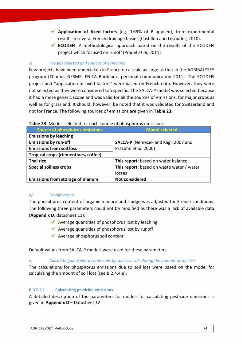
AGRIBALYSE®: Methodology 74
Application of fixed factors (eg. 0.69% of P applied), from experimental
results in several French drainage basins (Castillon and Lesouder, 2010).
ECODEFI: A methodological approach based on the results of the ECODEFI
project which focused on runoff (Pradel et al, 2011)
c) Models selected and sources of emissions
Few projects have been undertaken in France on a scale as large as that in the AGRIBALYSE®
program (Thomas NESME, ENITA Bordeaux, personal communication 2011). The ECODEFI
project and “application of fixed factors” were based on French data. However, they were
not selected as they were considered too specific. The SALCA-P model was selected because
it had a more generic scope and was valid for all the sources of emissions, for major crops as
well as for grassland. It should, however, be noted that it was validated for Switzerland and
not for France. The following sources of emissions are given in Table 23.
Table 23: Models selected for each source of phosphorus emissions
Source of phosphorus emissions Model selected
Emissions by leaching
SALCA-P (Nemecek and Kägi, 2007 and Prasuhn et al, 2006)
Emissions by run-off
Emissions from soil loss
Tropical crops (clementines, coffee)
Thai rice This report: based on water balance
Special soilless crops This report: based on waste water / water losses
Emissions from storage of manure Not considered
d) Modifications
The phosphorus content of organic manure and sludge was adjusted for French conditions.
The following three parameters could not be modified as there was a lack of available data
(Appendix D, datasheet 11):
Average quantities of phosphorus lost by leaching
Average quantities of phosphorus lost by runoff
Average phosphorus soil content
Default values from SALCA-P models were used for these parameters.
e) Calculating phosphorus emissions by soil loss: calculating the amount of soil lost
The calculations for phosphorus emissions due to soil loss were based on the model for calculating the amount of soil lost (see B.2.4.4.e).
B.3.5.11 Calculating pesticide emissions
A detailed description of the parameters for models for calculating pesticide emissions is given in Appendix D – Datasheet 12.
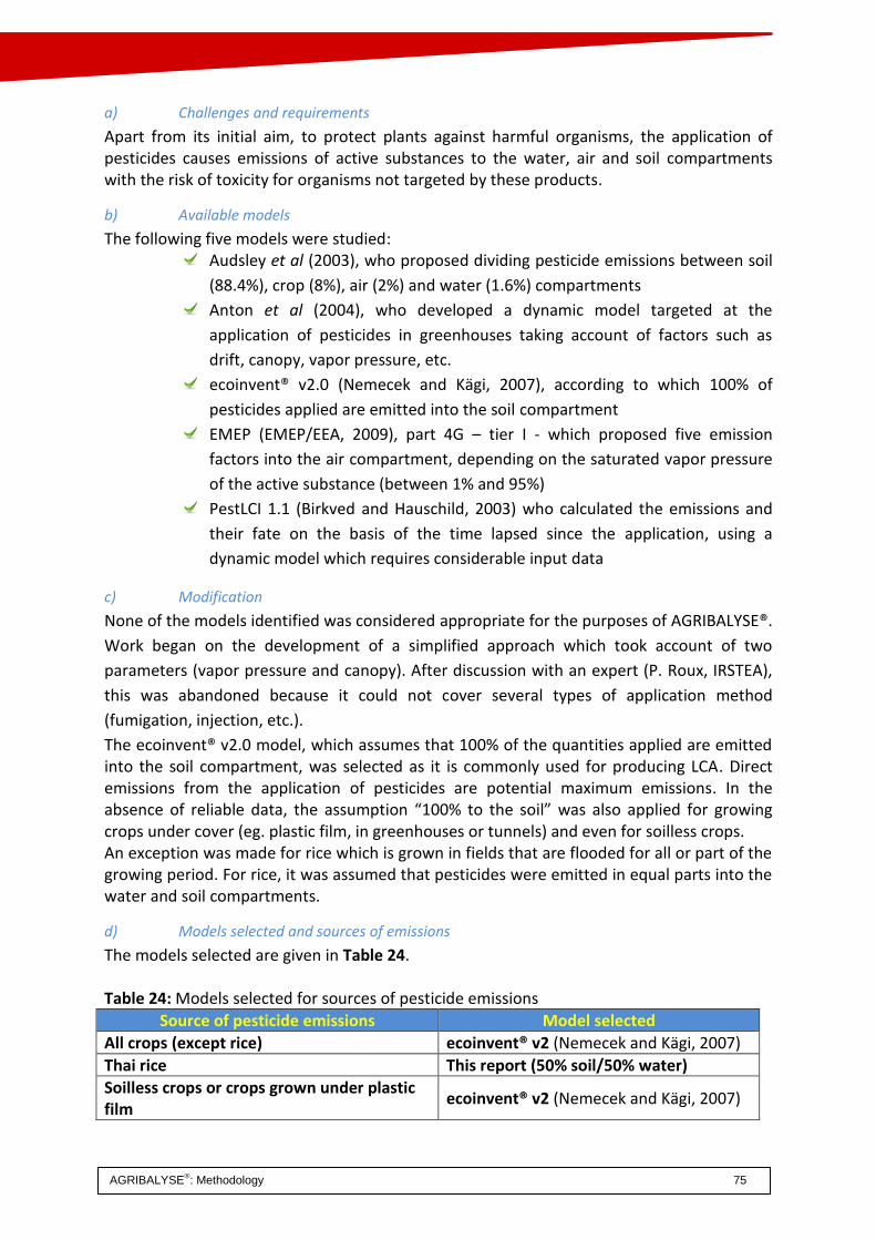
AGRIBALYSE®: Methodology 75
a) Challenges and requirements
Apart from its initial aim, to protect plants against harmful organisms, the application of pesticides causes emissions of active substances to the water, air and soil compartments with the risk of toxicity for organisms not targeted by these products.
b) Available models
The following five models were studied: Audsley et al (2003), who proposed dividing pesticide emissions between soil
(88.4%), crop (8%), air (2%) and water (1.6%) compartments
Anton et al (2004), who developed a dynamic model targeted at the
application of pesticides in greenhouses taking account of factors such as
drift, canopy, vapor pressure, etc.
ecoinvent® v2.0 (Nemecek and Kägi, 2007), according to which 100% of
pesticides applied are emitted into the soil compartment
EMEP (EMEP/EEA, 2009), part 4G – tier I - which proposed five emission
factors into the air compartment, depending on the saturated vapor pressure
of the active substance (between 1% and 95%)
PestLCI 1.1 (Birkved and Hauschild, 2003) who calculated the emissions and
their fate on the basis of the time lapsed since the application, using a
dynamic model which requires considerable input data
c) Modification
None of the models identified was considered appropriate for the purposes of AGRIBALYSE®.
Work began on the development of a simplified approach which took account of two
parameters (vapor pressure and canopy). After discussion with an expert (P. Roux, IRSTEA),
this was abandoned because it could not cover several types of application method
(fumigation, injection, etc.).
The ecoinvent® v2.0 model, which assumes that 100% of the quantities applied are emitted into the soil compartment, was selected as it is commonly used for producing LCA. Direct emissions from the application of pesticides are potential maximum emissions. In the absence of reliable data, the assumption “100% to the soil” was also applied for growing crops under cover (eg. plastic film, in greenhouses or tunnels) and even for soilless crops. An exception was made for rice which is grown in fields that are flooded for all or part of the growing period. For rice, it was assumed that pesticides were emitted in equal parts into the water and soil compartments.
d) Models selected and sources of emissions
The models selected are given in Table 24. Table 24: Models selected for sources of pesticide emissions
Source of pesticide emissions Model selected
All crops (except rice) ecoinvent® v2 (Nemecek and Kägi, 2007)
Thai rice This report (50% soil/50% water)
Soilless crops or crops grown under plastic film
ecoinvent® v2 (Nemecek and Kägi, 2007)

AGRIBALYSE®: Methodology 76
B.3.5.12 Calculating dinitrogen oxide emissions (N2O)
The emissions of N2O from agriculture are mainly due to the use of mineral and organic nitrogen amendments and the management of manure and slurry. The N2O emitted comes from the nitrification - denitrification process and is a major contributor to global warming. A detailed description of the parameters for models for calculating N2O emissions is given in Appendix D – Datasheet 13.
a) A) Challenges and requirements
In farming, N2O emissions mainly come from mineral and organic fertilizers and management of animal excretions.
b) Available models
Several models were identified in the literature: CORPEN (2003) and CORPEN (2006)
MELODIE (Chardon et al, 2011)
Nemecek and Kägi, 2007
EMEP/EEA, 2009
IPCC, 2006b
Daum and Schenck, 1996
c) Models selected and sources of emissions
The model selected for dinitrogen oxide emissions was that proposed by IPCC (2006b) which is internationally recognized by scientists. When Tier 2 emission factors were available they were used but, for several cases, Tier 1 had to be used. The models and sources of emissions for calculating N2O emissions are given in Table 25. Table 25: Models selected for each source of N2O emissions
Source of N2O emissions Model selected
Arable / horticultural production (agricultural soils)
IPCC 2006b, Tier 1 (for emission factors)1)
Special French crops IPCC 2006b, Tier 1 (for emission factors)1)
Tropical crops (clementines, coffee)
IPCC 2006b, Tier 1
Thai rice IPCC 2006b, Tier 2 based on Yan et al, 2003b
Grazing IPCC 2006b, Tier 1
Excretions in buildings/storage CORPEN 2006, 2003, 2001, 1999a and 1999b: for calculating the amount of nitrogen excreted by the animals
IPCC 2006b, Tier 2 for emission factors (and the fraction leached):
Excretions in outdoor runs IPCC 2006b, Tier 2 for emission factors (and the fraction leached)
1) Indirect N2O emissions were not calculated using the default leached and volatilized fractions in IPCC but by calculating the quantities leached and volatilized using nitrate and ammonia models.

AGRIBALYSE®: Methodology 77
Daum and Schenck (1996) analyzed the volatilization of N2O for soilless crops. As the emission factor they proposed was close to that of IPCC (2006b) and it has large uncertainties, the N2O flow estimation method used for agricultural soils was finally selected.
B.3.5.13 Water usage
For producing an LCA, water has until now been considered as a potential receptor of polluting emissions. The quality of the water is taken into account, in particular with categories of impact on eutrophication, acidification and ecotoxicity. However, water has not as yet been taken into account as a resource. Recent methodological developments are able to take account of the impact of water consumption. A bibliographic study carried out by CIRAD identified the method developed by Pfister et al (2009) as currently the most efficient (Appendix F). The data required to implement this method is the amount of water consumed by the production processes. However, as this information was not available from the various data sets used for the AGRIBALYSE® product inventory, the method developed by Pfister et al (2009) could not be used.
B.3.5.14 Calculating emissions of phosphorus , nitrogen and total suspended solids from fish
farms
A detailed description of the parameters for calculating N, P and TSS emissions from fish farms is given in Appendix D – Datasheet 14.
a) Challenges and requirements
Given the special nature of the farming methods, fish farms have a potentially significant impact on the environment, in particular for eutrophication. A more accurate estimate is, therefore, required of the TTS, nitrogen and phosphorus emissions in dissolved and particulate form, using specific models.
b) Models selected and sources of emissions
Models of phosphorus, nitrogen and TSS emissions have been developed specifically for French fish farms (Papatryphon et al, 2005). The models selected for calculating this parameter are given in Table 26.
Table 26: Models selected for each substance emitted by fish farms
Source of emissions Model selected
Nitrogen
Papatryphon et al, 2005 Phosphorus
Total suspended solids (TSS)
The model selected is based on the principle of a balance between inputs and outputs required a knowledge of the composition of the food rations distributed to the fish, the composition of the fish (the trace elements in each tissue) and the quantity of undigested nutrients.

AGRIBALYSE®: Methodology 78
B.4 Allocation of flows and emissions
B.4.1 Allocation of shared inputs: infrastructure
The infrastructure requirements for farming were taken into account by allocating the impacts of the infrastructure pro rata for the operation time (for arable / horticultural agricultural processes) or pro rata for the time the area required is occupied (for buildings). The operation time covers the time required to do the work and the preparation. This is a standard approach for agricultural product LCAs (Nemecek and Kägi, 2007; Gac et al, 2010).
B.4.2 Allocation to co-products
AGRIBALYSE® is limited to agricultural production. With the exception of certain processes carried out on the farm (eg: haylage, silage, etc), processing “on the farm” and “post farm” is not considered. Co-products such as press cake, from post farm processing, are not within the scope of AGRIBALYSE®. Certain co-products were, however, evaluated using existing studies for the whole of the processing stage but only where the co-products were used for animal feed (Appendix L).
B.4.2.1 Definition of “co-product”
Agricultural production systems are often used for several purposes and a single production system may provide several co-products. The “main product” is defined in AGRIBALYSE® as the output from the main production of the system considered. All other outputs produced by the system were defined as co-products.
B.4.2.2 Principles and choices
a) Basic rule
As a general rule, AGRIBALYSE® complies with international standards. Whatever the allocation rule selected, it must apply equally to the main product and to co-products. In all cases, the allocation procedure is described in detail.
b) Hierarchy
The allocation rules are based on the recommendations in the interpretation note (guide de lecture) for the methodology appendix of the BPX 30-323 manual (AFNOR, 2011). In accordance with ISO 14044 (ISO, 2006b), in AGRIBALYSE® the following general hierarchy is used for the allocation methods:
Option 1: Wherever possible, allocation should be avoided by:
dividing the unit process to be allocated into two or more subprocesses and
collecting the input and output data related to these sub-processes, or
By expanding the product system to include the additional functions related
to the co-products, taking into account of the requirements of 4.2.3.3 of ISO
14044 (ISO, 2006b). This is not an option for attributional LCI databases such
as AGRIBALYSE®.
Option 2. Physical allocation. The inputs and outputs of the system should be
partitioned between its different products or functions in a way that reflects the
underlying physical relationships between them, i.e. they should reflect the way in

AGRIBALYSE®: Methodology 79
which the inputs and outputs are changed by quantitative changes in the products or
functions delivered by the system.
Option 3. Economic allocation. The economic value of the co-products (eg. the
market value) represents the production goal. This allocation method is commonly
used in LCA when there is no physical criterion that is relevant for the product or for
the co-products. The disadvantage of this allocation method is that the impact of the
products depends on the market and may vary significantly from year to year even
though the production system remains the same.
To overcome this problem, the values are smoothed over 5 years excluding the
highest and lowest values (Olympic average). This method gives the value of a
product and how the market value changes excluding major price swings.

AGRIBALYSE®: Methodology 80
c) AGRIBALYSE® products / co-products
Table 27 gives an overview of the products / co-products for each product type and the methods for allocating the flows between product and co-products. These methods are described in the following chapters (B.3.2.3 to B.3.2.5). Table 27: Products / co-products generated in AGRIBALYSE® – Method selected for handling co-products
Product type Product / Co-
product
Method selected for handling co-
products
Arable / horticultural
Cereals / protein crops
Grain straw
Economic
Carrots Marketable carrots Waste
100% Not considered
Orchards / Grapevines Fruit Prunings
100% Not considered
Grassland Grazed grass Hay
Weight
Clementines Clementines, export Clementines, local
Economic
Coffee Green coffee seed (main product) Pulp (composted on plantation)
Economic 96% 4%
Livestock
Suckling beef Young bulls / heifers Cull cows
Bio-physical
Dairy cattle Milk Cull cows Calves
Bio-physical
Sheep (meat) Lambs Wool Cull sheep
Bio-physical
Sheep (milk) Milk Lambs Wool Cull sheep
Bio-physical
Goats (milk) Milk Cull goats
Bio-physical
Layers Eggs Cull poultry
Bio-physical
Pigs Pork Cull sows
Bio-physical

AGRIBALYSE®: Methodology 81
B.4.2.3 French crops
a) Grain / straw (cereals, protein crops)
It was decided to use economic allocation for straw as a co-product of grain. However, as the straw market is currently not very structured, the data on the economic value of this co-product is not very reliable. Consequently, no value was allocated to the straw and 100% of the impact was allocated to the grain. An exception was done concerning biogenic CO2, a mass allocation was performed to account for the real carbon flow. Note: The straw market may one day become more structured or more reliable, representative data may become available. Selecting economic allocation makes it possible to take account of this data in an update to the AGRIBALYSE® database.
b) Marketable carrots – Carrot waste
In accordance with the allocation rules for the other products, no allocation was made for waste. The carrot yield included top grade carrots (for the fresh vegetable market) and second grade carrots (for industrial processing). Not distinguishing between these two outputs is equivalent to mass allocation, i.e. the two types of carrot have the same impact.
c) Peaches/nectarines, apples / cider apples – wood; grapes for wine - wood
As the wood and prunings from orchards are usually burned in the field, the wood is not considered as a co-product leaving the field and so no allocation is required. As for carrots, the yield from apples includes second grade apples for industrial processing.
d) Grass for hay / silage and grazed grass
The grassland LCI data sets include five LCI data sets for grass grazed by cattle and twelve cut grass LCI data sets with both cutting and grazing. Some of the grass is stored (hay, haylage, silage) and considered to be the main product of the LCI. The other part is grazed for the period of the inventory and considered as a co-product. Mass allocation was used for the flows related to pasture seeding and fertilizing, on the basis that the protein and energy content of the grass was roughly the same whether the grass was grazed or harvested to be preserved. Flows due to harvesting were fully allocated to stored grass.The “grazed grass” co-products were not included in the AGRIBALYSE® database as there were five LCI data sets for full grazing (cattle) and no use of these co-product data sets was envisaged.
B.4.2.4 Tropical crops
a) Export grade clementines – Local market grade clementines
Economic allocation was used between local market grade clementines and export grade clementines. Wood from prunings in Moroccan clementine orchards was not considered as a co-product leaving the plot. This wood was generally shredded and spread on the ground between rows and so no allocation was required.
b) Coffee – wood
Some of the wood from pruning in coffee plantations is left in situ and some is used for heating. As this wood has no market value, no impacts were allocated to it.

AGRIBALYSE®: Methodology 82
B.4.2.5 Livestock production
For livestock production, the impacts were allocated to the related products using a “bio-physical” model (Figure 14). Initially, allocation was avoided by dividing the process into several unit processes, breaking the life of the animal down into characteristic development stages. For certain stages, there were always several products, and so an allocation had to be made, for example for the milk production phase for cattle. An allocation for milk/calves had to be made. This was done pro rata for the energy required for the various physiological functions of the animal and to produce the product and co-products. Five functions were defined: maintenance, activity, growth, lactation and gestation. LCI « Animal of 0 day » (ex : “Calf of 0 day”) correspond to phases required to build « young animals for meat » LCIs and replacing animals. These LCIS are not final product at farm gate (unlike “Calf, conventional […]/FR”) and can’t be used as such.
Figure 14: Allocation of impacts to co-products using a “bio-physical” model for a dairy farm: blue is the development stages for which the impacts are allocated to the cull cow and green for the stages for which the impacts are allocated to milk and calves. The impacts between milk and calves are allocated pro rata to the energy required to produce these two products.
Appendix M gives the allocation factors used in AGRIBALYSE®.
Cull cow
Environmental impacts
Environmental impacts
Milk Calf
Milk
Calf
• Lactation (Maintenance + Activity) * (1-(Gestation/ Lactation)
• Gestation (Maintenance + Activity) * (Gestation/ Lactation)
Calf birth - weaning
Replacement heifer weaning –
1 year
Replacement heifer – 1 - 2
years
Replacement heifer – over 2
years
Cull cow at end of life
Dairy cow in full production
Environmental impacts

AGRIBALYSE®: Methodology 83
a) Dairy cattle
Table 28: Development stages, output products and physiological functions of dairy cattle, for allocating environmental impacts depending on the energy required for these functions
Stage Output
products
Mai
nte
nan
ce
Act
ivit
y
Gro
wth
Lact
atio
n
Ges
tati
on
Comments
Calf 0-weaning Cull cow X X X Mass allocation, pro rata to live weight of
product Calf (b) X X X
Heifer Weaning-1 yr
Cull cow X X X
Heifer 1-2 yrs Cull cow X X X
Heifer + 2 yrs Cull cow X X X
Dairy cow in production
Milk X X X 𝐿𝑎𝑐𝑡𝑎𝑡𝑖𝑜𝑛 + (𝑀𝑎𝑖𝑛𝑡𝑒𝑛𝑎𝑛𝑐𝑒 + 𝐴𝑐𝑡𝑖𝑣𝑖𝑡𝑦) ∗ (1 −𝐺𝑒𝑠𝑡𝑎𝑡𝑖𝑜𝑛
𝐿𝑎𝑐𝑡𝑎𝑡𝑖𝑜𝑛)
Calf at birth X X X 𝐺𝑒𝑠𝑡𝑎𝑡𝑖𝑜𝑛 + (𝑀𝑎𝑖𝑛𝑡𝑒𝑛𝑎𝑛𝑐𝑒 + 𝐴𝑐𝑡𝑖𝑣𝑖𝑡𝑦) ∗𝐺𝑒𝑠𝑡𝑎𝑡𝑖𝑜𝑛
𝐿𝑎𝑐𝑡𝑎𝑡𝑖𝑜𝑛
Cull cow
Cull cow at end of life
Cull cow X X X
X is the functions concerned for each development stage.
It was assumed that the weight gain for the animal in the dairy cow in production stage was negligible. Consequently, all the impacts were allocated between the calves and the milk (Table 28).
b) Beef cattle -Sucklers
Table 29: Development stages, output products and functions of suckler cows for allocating impacts depending on the energy required for these functions
Stage Output products
Mai
nte
nan
ce
Act
ivit
y
Gro
wth
Lact
atio
n
Ge
stat
ion
Calf 0-1 year Heifer and beef X X X
Replacement heifer 0-1 yr Cull cow X X X
Replacement heifer 1-2 yrs Cull cow X X X
Replacement heifer +2 yrs Cull cow X X X
Suckler cow Calf at birth x x x X X
Cull cow at end of life Cull cow X X X
Genitor Cull cow X X X X is the functions concerned for each development stage
During the suckler cow in production stage, the weight gain of the animal is not negligible and so the impacts were allocated between the cull cow and the heifers (Table 29).
c) Beef cattle - Fattening
The impacts of all classes of animals were allocated to the fattened steer.

AGRIBALYSE®: Methodology 84
d) Milk goats
Table 30: Development stages, output products and functions of milk goats for allocating impacts depending on the energy required for these functions
Stage Output
products
Mai
nte
nan
ce
Act
ivit
y
Gro
wth
Lact
atio
n
Ges
tati
on
Comments
Kid (0 - 8 days) Cull goat X X X
Replacement kid 0-1 yr
Cull goat X X X
Goat in production
Cull goat
Kid X X X X 𝐺𝑒𝑠𝑡𝑎𝑡𝑖𝑜𝑛 + (𝑀𝑎𝑖𝑛𝑡𝑒𝑛𝑎𝑛𝑐𝑒 + 𝐴𝑐𝑡𝑖𝑣𝑖𝑡𝑦) ∗𝐺𝑒𝑠𝑡𝑎𝑡𝑖𝑜𝑛
𝐿𝑎𝑐𝑡𝑎𝑡𝑖𝑜𝑛
Milk X X X X 𝐿𝑎𝑐𝑡𝑎𝑡𝑖𝑜𝑛 + (𝑀𝑎𝑖𝑛𝑡𝑒𝑛𝑎𝑛𝑐𝑒 + 𝐴𝑐𝑡𝑖𝑣𝑖𝑡𝑦) ∗
(1 −𝐺𝑒𝑠𝑡𝑎𝑡𝑖𝑜𝑛
𝐿𝑎𝑐𝑡𝑎𝑡𝑖𝑜𝑛)
X is the functions concerned for each development stage
During the milk goat in production stage, it was assumed that the weight gain of the animal was negligible and so all the impacts were allocated to the kids and the milk (Table 30).
e) Sheep for meat
Cull sheep, lambs and wool were defined as co-products. The impacts were allocated as shown in Table 31. Table 31: Development stages, output products and functions of sheep for meat for allocating impacts depending on the energy required for these functions
Stage Output products
Mai
nte
nan
ce
Act
ivit
y
Gro
wth
Lact
atio
n
Ge
stat
ion
Wo
ol
pro
du
ctio
n
Lamb 0-weaning Cull ewe X X X
Replacement gimmer weaning-1 yr Cull ewe X X X
Wool X
Weaned lamb for sale Lambs X X X X
Replacement gimmer 1-2 yrs Cull ewe X X X
Wool X
Ewe in production
Cull ewe X X X
Lambs X X
Wool X X is the functions concerned for each development stage
During the ewe in production stage, the weight gain of the animal is not negligible and so the impacts were allocated to the cull ewes and the lambs.
f) Sheep for milk
Milk, cull ewes, lambs and wool were identified as co-products. The impacts were allocated as shown in Table 33.

AGRIBALYSE®: Methodology 85
Table 32: Development stages, output products and functions of milk sheep for allocating impacts depending on the energy required for these functions
Stage Output
products
Mai
nte
nan
ce
Act
ivit
y
Gro
wth
Lact
atio
n
Ges
tati
on
Wo
ol
pro
du
ctio
n
Comments
Lamb (0-weaning) Cull ewe X X X
Replacement gimmer 0-1 yr
Cull ewe X X X
Wool X
Replacement gimmer 1-2 yrs
Cull ewe X X X
Wool X
Ewe in production
Cull ewe
Lamb X X X 𝐺𝑒𝑠𝑡𝑎𝑡𝑖𝑜𝑛 + (𝑀𝑎𝑖𝑛𝑡𝑒𝑛𝑎𝑛𝑐𝑒 +
𝐴𝑐𝑡𝑖𝑣𝑖𝑡𝑦) ∗𝐺𝑒𝑠𝑡𝑎𝑡𝑖𝑜𝑛
𝐿𝑎𝑐𝑡𝑎𝑡𝑖𝑜𝑛
Milk X X X 𝐿𝑎𝑐𝑡𝑎𝑡𝑖𝑜𝑛 + (𝑀𝑎𝑖𝑛𝑡𝑒𝑛𝑎𝑛𝑐𝑒 +
𝐴𝑐𝑡𝑖𝑣𝑖𝑡𝑦) ∗ (1 −𝐺𝑒𝑠𝑡𝑎𝑡𝑖𝑜𝑛
𝐿𝑎𝑐𝑡𝑎𝑡𝑖𝑜𝑛)
Wool X
X is the functions concerned for each development stage
For the milk ewe phase, it was assumed that the weight gain of the animal was negligible and so all the impacts were allocated to the lambs and the milk.
g) Layers
Table 33: Development stage, output and percentage of impact of stage allocated to each product for layers
Stage Output Percentage of impacts allocated to product
Chick - For reproduction
Cull hen 100
Hen - Reproduction
Cull hen 100
Chicken Cull hen 100
Layer Cull hen 0
egg 100
For layers, it was assumed that the weight gain of the animal was negligible. The
environmental impacts were allocated to the eggs (Table 33).
h) Rabbits
Table 34: Development stages, output products and physiological functions of rabbits for allocating environmental impacts depending on the energy required for these functions
Stage Output products
Mai
nte
nan
ce
Act
ivit
y
Gro
wth
Lact
atio
n
Ges
tati
on
Rabbit - Doe Cull rabbit X X X
Rabbit (kit) X X
Rabbit - Fattening Rabbit X X X

AGRIBALYSE®: Methodology 86
i) Pigs
For pig production, the impacts were allocated to the piglets and the cull sows depending on the amount of feed used (Table 35). Table 35: Development stage, product and allocation of the environmental impacts for pigs
Stage Output Allocation of impacts
Pig - Sows Cull sows
0.75*Qty feed sow in gestation + 0.4*Qty feed sow suckling + 1*Qty feed gilt
Pig for pork (piglets)
0.25*Qty feed sow in gestation + 0.6*Qty feed sow suckling
Pig - Post weaning
Pig for pork 100% for pig for pork
Pig - Fattening Pig for pork 100% for pig for pork Note: Qty = Quantity
B.4.3 Allocation of processes, inputs and outputs for cropping sequences
B.4.3.1 Principles and allocations for cropping sequences in the AGRIBALYSE database®
It is difficult to allocate the impacts of a production system to each crop in a cropping sequence because: - Certain practices may involve several crops in the rotation system, - Certain emissions depend on the practices and characteristics associated with a crop as well as on the practices and characteristics associated with previous or following crops. The ILCD Handbook recommends taking account of the nutrients remaining in the system after a crop has been harvested as a co-product of this crop and continue by extending the system or by allocation. The allocation rules used for AGRIBALYSE® are given below.
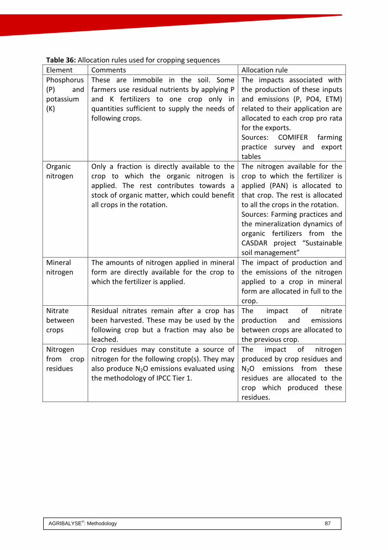
AGRIBALYSE®: Methodology 87
Table 36: Allocation rules used for cropping sequences
Element Comments Allocation rule
Phosphorus (P) and potassium (K)
These are immobile in the soil. Some farmers use residual nutrients by applying P and K fertilizers to one crop only in quantities sufficient to supply the needs of following crops.
The impacts associated with the production of these inputs and emissions (P, PO4, ETM) related to their application are allocated to each crop pro rata for the exports. Sources: COMIFER farming practice survey and export tables
Organic nitrogen
Only a fraction is directly available to the crop to which the organic nitrogen is applied. The rest contributes towards a stock of organic matter, which could benefit all crops in the rotation.
The nitrogen available for the crop to which the fertilizer is applied (PAN) is allocated to that crop. The rest is allocated to all the crops in the rotation. Sources: Farming practices and the mineralization dynamics of organic fertilizers from the CASDAR project “Sustainable soil management”
Mineral nitrogen
The amounts of nitrogen applied in mineral form are directly available for the crop to which the fertilizer is applied.
The impact of production and the emissions of the nitrogen applied to a crop in mineral form are allocated in full to the crop.
Nitrate between crops
Residual nitrates remain after a crop has been harvested. These may be used by the following crop but a fraction may also be leached.
The impact of nitrate production and emissions between crops are allocated to the previous crop.
Nitrogen from crop residues
Crop residues may constitute a source of nitrogen for the following crop(s). They may also produce N2O emissions evaluated using the methodology of IPCC Tier 1.
The impact of nitrogen produced by crop residues and N2O emissions from these residues are allocated to the crop which produced these residues.

AGRIBALYSE®: Methodology 88
B.4.3.2 Allocation of organic N, P and K inputs on the basis of the 2006 Agreste farming
practices survey
Organic N, P and K inputs were allocated to all crops in a cropping sequence. This type of allocation required a detailed knowledge of the fertilizers applied and the yield for each of crops in the rotation system. There was little statistical data for cropping sequences and what information was available did not cover the production of all the crops studied in AGRIBALYSE®. The 2006 Agreste farming practices survey covered crops and not cropping sequences. However, it had the advantage of covering most of the main production regions for about ten major crops. It also gave information on the history for each plot and in particular details of previous crops. The year 2006 was considered representative of fertilizer applications during the reference period 2001-2005. The succession of crops grown in the 14,000 plots studied was known for the period 2001 to 2005. An analysis of this data showed nearly 4,000 different cropping sequences. This diversity and the size of the samples did not make it possible to reconstitute fertilization practices for each type of cropping sequence. To take account of this diversity, these rotation systems were grouped together as “cropping sequence groups” using appropriate statistical optimal matching methods (Gabadinho et al, 2011). The 4,000 rotation systems were grouped into 34 major cropping sequence groups, depending on the dominant crops and production region (Jouy and Wissocq, 2011). This made it possible to take account of the differences in the application of fertilizers for a given crop depending on the rotation system and region, based on Agreste 2006 data. After allocation according to the rules in Table 36 for each crop within the cropping sequence groups, a French average was calculated.
The implementation of this approach in the LCI data sets is given in Appendix D – Datasheet 16.

AGRIBALYSE®: Methodology 89
Part C – Impact assessment
AGRIBALYSE did not work on developping caracterization methods. Following update v1.2, it was decided not to provide any specific caracterisation method along with AGRIBALYSE. This will enable users to choose the caracterisation method most suitable for there needs and most up to date. However users should always check that all the flows provided by AGRIBALYSE are characterized in the method they use. In order to provide impact indicators to users without LCA softwares, most common ILCD mid point indicators were selected for the excel file, with seven extra common indicators related to energy/resource use. For “water resource depletion” and “particule matter”, direct emissions are not accounted for in AGRIBALYSE. Tableau 37 : Impact categories in the Excel summary files. Categories identified by * means that not all flows are not considered for these categories, thus these indicators should not be analyzed.(Table based on the description of characterization methods in SimaPro 8.03)
Catégorie d'impacts selon ILCD
Unité Description Source
Climate change kg CO2 eq Global Warming Potential calculating the radiative forcing over a time horizon of 100 years
IPCC 2007
Ozone depletion kg CFC-11 eq
Calculating the destructive effects on the stratospheric ozone layer over a time horizon of 100 years.
World Meteorological Organization (WMO) 1999.
Human toxicity, cancer effects
CTUh expressing the estimated increase in morbidity in the total human population per unit mass of a chemical emitted (cases per kilogramme). Specific groups of chemicals requires further works.
USEtox
Human toxicity, non-cancer effects
CTUh expressing the estimated increase in morbidity in the total human population per unit mass of a chemical emitted (cases per kilogramme). Specific groups of chemicals requires further works
USEtox
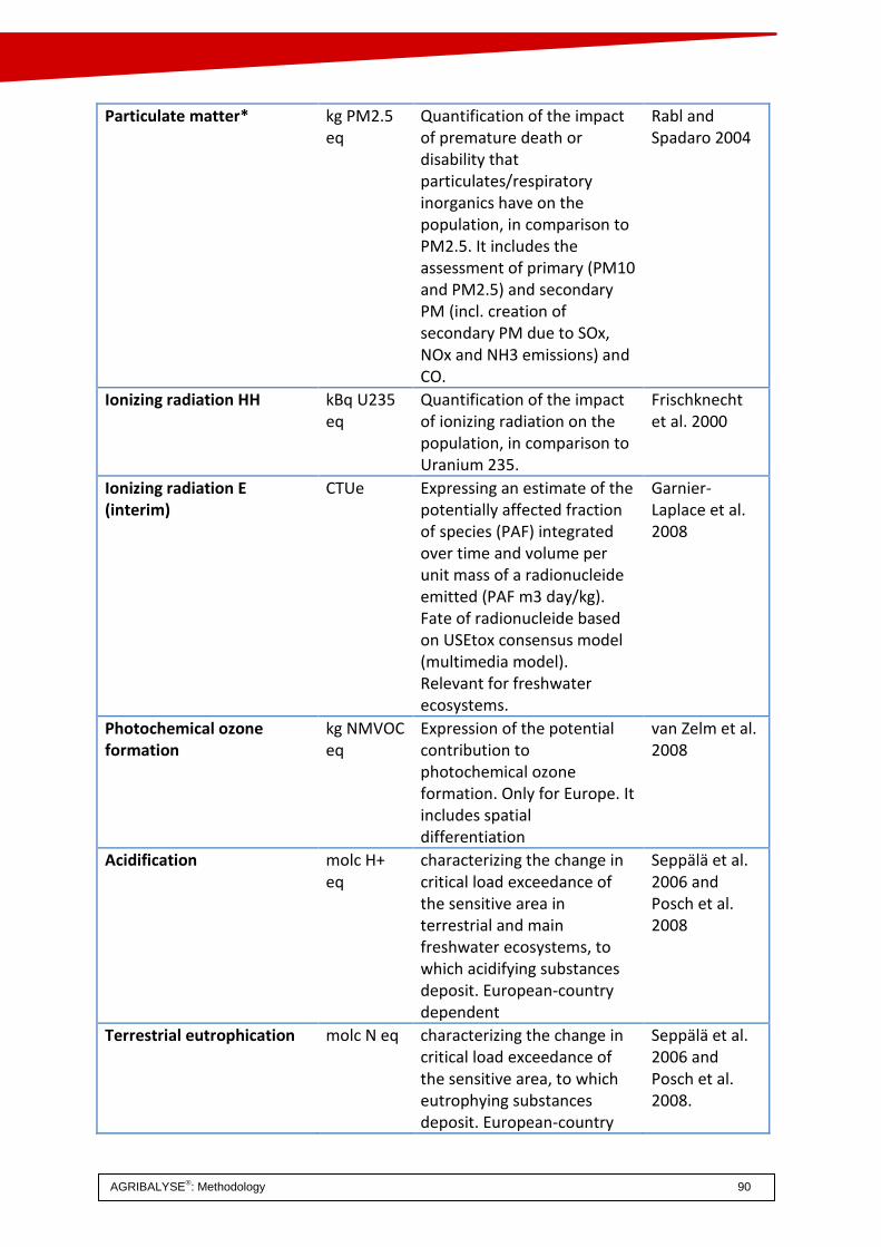
AGRIBALYSE®: Methodology 90
Particulate matter* kg PM2.5 eq
Quantification of the impact of premature death or disability that particulates/respiratory inorganics have on the population, in comparison to PM2.5. It includes the assessment of primary (PM10 and PM2.5) and secondary PM (incl. creation of secondary PM due to SOx, NOx and NH3 emissions) and CO.
Rabl and Spadaro 2004
Ionizing radiation HH kBq U235 eq
Quantification of the impact of ionizing radiation on the population, in comparison to Uranium 235.
Frischknecht et al. 2000
Ionizing radiation E (interim)
CTUe Expressing an estimate of the potentially affected fraction of species (PAF) integrated over time and volume per unit mass of a radionucleide emitted (PAF m3 day/kg). Fate of radionucleide based on USEtox consensus model (multimedia model). Relevant for freshwater ecosystems.
Garnier-Laplace et al. 2008
Photochemical ozone formation
kg NMVOC eq
Expression of the potential contribution to photochemical ozone formation. Only for Europe. It includes spatial differentiation
van Zelm et al. 2008
Acidification molc H+ eq
characterizing the change in critical load exceedance of the sensitive area in terrestrial and main freshwater ecosystems, to which acidifying substances deposit. European-country dependent
Seppälä et al. 2006 and Posch et al. 2008
Terrestrial eutrophication molc N eq characterizing the change in critical load exceedance of the sensitive area, to which eutrophying substances deposit. European-country
Seppälä et al. 2006 and Posch et al. 2008.

AGRIBALYSE®: Methodology 91
dependent
Freshwater eutrophication kg P eq Expression of the degree to which the emitted nutrients reaches the freshwater end compartment (phosphorus considered as limiting factor in freshwater). European validity. Averaged characterization factors from country dependent characterization factors.
ReCiPe version 1.05.
Marine eutrophication kg N eq Expression of the degree to which the emitted nutrients reaches the marine end compartment (nitrogen considered as limiting factor in marine water). European validity. Averaged characterization factors from country dependent characterization factors.
ReCiPe version 1.05
Freshwater ecotoxicity CTUe Comparative Toxic Unit for ecosystems (CTUe) expressing an estimate of the potentially affected fraction of species (PAF) integrated over time and volume per unit mass of a chemical emitted (PAF m3 day/kg). Specific groups of chemicals requires further works
USEtox
Land use kg C deficit
based on changes in SOM, measured in (kg C/m2/a). Biodiversity impacts not covered by the data set.
Mila i Canals et al. 2007.
Water resource depletion* m3 water eq
Water resource depletion: Freshwater scarcity: Scarcity-adjusted amount of water used.
Swiss Ecoscarcity 2006
Mineral, fossil & ren resource depletion
kg Sb eq Scarcity of mineral resource with the scarcity calculated as 'Reserve base'. It refers to identified resources that meets specified minimum physical and chemical criteria related to current mining
van Oers et al. 2002

AGRIBALYSE®: Methodology 92
practice. The reserve base may encompass those parts of the resources that have a reasonable potential for becoming economically available within planning horizons beyond those that assume proven technology and current economics.
Extra indicators (non ILCD)
Non renewable, fossil MJ Cumulative Energy Demand (CED) required to produce the good/service.
CED 1.8
Non renewable nuclear MJ Cumulative Energy Demand (CED) required to produce the good/service.
CED 1.8
Non-renewable, biomass MJ Cumulative Energy Demand (CED) required to produce the good/service.
CED 1.8
Renewable, biomass MJ Cumulative Energy Demand (CED) required to produce the good/service.
CED 1.8
Renewable, wind, solar, geothe
MJ Cumulative Energy Demand (CED) required to produce the good/service.
CED 1.8
Renewable water MJ Cumulative Energy Demand (CED) required to produce the good/service.
CED 1.8
Land competition M2 Land area required to produce the good/service. Permet de connaitre la quantité d’espace necessaire à la production du bie/service.
CML 2001

AGRIBALYSE®: Methodology 93
Part D – Conclusion
This report sets out all the choices made for building the AGRIBALYSE® LCI data sets. It explains how the data was obtained, simplifies the production of LCI data sets similar to those in AGRIBALYSE® and helps to interpret the results. It is not intended to be a guide although it may help to harmonize the selection of methodologies for LCA of agricultural products in France or abroad. New versions of this report may be issued depending on how the AGRIBALYSE® database develops.

AGRIBALYSE®: Methodology 94
Bibliography
Below is a list of all the works cited in the main part of this report and in the appendices. ACTA, 2005. Index phytosanitaire 2005, ACTA, 2005.
ACTA, 2009. Index phytosanitaire 2005, ACTA, 2009.
ADEME, 2008. Bibliographic review of “Life cycle analyses of agricultural products” studies. Overview. Study carried out by ECOINTESYS on behalf of ADEME.
AFNOR, 2011. BPX 30-323-0 : Affichage environnemental des produits de grande consummation – Principes généraux et cadre méthodologique. Ed AFNOR, La Plaine Saint-Denis, France. http://www.boutique.afnor.org/norme/bp-x30-323-4/principes-generaux-pour-l-affichage-environnemental-des-produits-de-grande-consommation-partie-4-methodologie-d-evaluation-d/article/619574/fa174367#info
AGRESTE, 2012. Annual crop statistics – Land occupation (1990-2010).
http://agreste.agriculture.gouv.fr/page-d-accueil/article/donnees-en-ligne.
AGRESTE, 2008. Poultry production avicole survey.
http://www.agreste.agriculture.gouv.fr/enquetes/productions-animales-625/aviculture-471/
AGRESTE, 2006. 2006 farming practices survey. http://agreste.agriculture.gouv.fr/page-d-
accueil/article/donnees-en-ligne.
Agri-footprint, 2011. Agri-footprint. Dynamic environmental knowledge base for agri and food products. Website funded by the Dutch Ministries of the Environment and Agriculture, and by Agentschap NL (the ADEME in the Netherlands). https://www.agrifootprint.co.
Alva A.K. and Larsen S., 1984. Phosphate Dynamics in an Acid Sulfate Soil under Flooded Condition Studied By a Tracer Technique. Royal Veterinary and Agricultural University Copenhagen, Denmark
ANSES, 2008. Table Ciqual - Composition nutritionnelle des aliments. http://www.afssa.fr/TableCIQUAL
Anton A., Castells F., MonteroJ.I. and Huijbergts M., 2004. Comparison of toxicological impacts of integrated and chemical pest management in Mediterranean greenhouses. Chemosphere 54 (8), 1225-1235.
Audsley E., Alber S., Clift R., Cowell S., Crettaz P., Gaillard G., Hausheer J., Jolliett O., Kleijn R., Mortensen B., Pearce D., Roger E., Teulon H., Weidema B. and van Zeijts H., 2003. Harmonization ofEnvironmental Life Cycle Assessment For Agriculture. European Commission. DG VI. Agriculture. Concerted Action AIR3-CT94-2028. Ed European Commission, Luxembourg, Luxembourg. p101.
Arrouays D., Balesdent J., Germon J-C., Jayet P-A., Soussana J-F. and Stengel P., 2002. Contribution à la lutte contre l’effet de serre. Stocker du carbone dans les sols agricoles de France ? Expertise collective. Synthèse du rapport. Ed INRA, Paris, France. p32.
Arvalis, 1998. Synthèse des résultats de l’enquête sur les ETM du blé tendre, du blé dur, du pois protéagineux et de la pomme de terre récoltés en 1997 et 1998.
Baize D., Deslais W. and Saby N., 2007. Teneurs an huit éléments traces (Cd, Cr, Cu, Hg, Ni, Pb, Se, Zn) dans les sols agricoles en France - Résultats d'une collecte de données à l'échelon national. Rapport final simplifié. Ed ADEME, Angers France. p 49.
Basset-Mens C., van der Werf H.M.G., Robin P., Morvan Th., Hassouna M., Paillat J‐M. and Vertès F., 2007. Methods and data for the environmental inventory of contrasting pig production systems. Journal of Cleaner Production 15, 1395‐1405.

AGRIBALYSE®: Methodology 95
Bayart J.B. and Aoustin E., 2011. The Water Impact Index, a simplified single indicator for water footprinting. LCM 2011 - Towards Life Cycle Sustainability Management, Berlin, Conference presentation.
Bayart J-B., Bulle C., Koehler A., Margni M., Pfister S., Vince F. and Deschenes L., 2010. A framework for assessing off stream freshwater use in LCA. International Journal of Life Cycle Assessment, 15, 439-453.
Beck T., Bos U., Wittstock B., Baitz M., Fischer M. and Sedlbauer K., 2008. LANCA land Use Indicator Value Calculator in Life Cycle Assessment – Methodological Report. Frauenhofer Institute for Building Physics, Echterdingen, Germany. p69.
Benoist, A., 2009. Eléments d’adaptation de la méthodologie d’analyse de cycle de vie aux carburants végétaux : Cas de la première génération. Thèse de doctorat, Mines ParisTech. p232.
Berger M. and Finkbeiner M., 2010. Water Footprinting: How to Address Water Use in Life Cycle Assessment?. Sustainability, 2 (4), 919-944.
Bessou C., Basset-Mens C., Tran T., Benoist A. (2013) LCA applied to perennial cropping systems: a
review focused on the farm stage. The International Journal of Life Cycle Assessment
18(2)340-361. DOI:10.1007/s11367-012-0502-z
Biard Y., Koch P. and Salou T., 2011a. AGRIBALYSE® : Guide de collecte – Version 5.0. Ed ADEME, Angers, France. p47.
Biard Y., Koch P. and Salou T., 2011b. AGRIBALYSE® : Manuel de l’OIS – Version 7.0. Ed ADEME, Angers, France. p51.
BIO IS, 2010. Elaboration d’un plan de développement d’une base publique de données d’ACV comme support à l’affichage. Study commissioned by ADEME – Confidential.
Birkved M. and Hauschild M., 2003. PESTLCI – A Pesticide Distribution Model For LCA. Institute for producte developpement, Technial University of Denmark, Lyngby, April 2003.
Bossard M., Feranec J. and Otahel J., 2000. CORINE land cover technical guide. Addenum 2000. 40. Ed European Environment Agency (EEA), Copenhagen, Danemark, from, http://ect.satellus.se/I&CLC2000/download.htm.
Boulard T., Raeppel C., Brun R., Lecompte F., Hayer F. and Gaillard G., 2011. Evaluation environnementale de la production de tomate en serre en France. 6ème Rencontres du végétal, 10-11/01/11. Agrocampus Ouest, centre d'Angers.
Brentrup F., Küsters J., Lammel J. and Kuhlmann H., 2000. Methods to estimate on-field nitrogen emissions from crop production as an input to LCA studies in the agricultural sector. Int. J. LCA. 5: 349-357.
Brisson N., Mary B., Ripoche D, Jeuffroy M-H., Ruget F., Nicoullaud B., Gate P., Devienne-Barret F., Antonioletti R., Durr C., Richard G., Beaudoin N., Recous S., Tayot X., Plenet D., Cellier P., Machet J-M., Meynard J-M. and Delécolle R., 1998. STICS: a generic model for the simulation of crops and their water and nitrogen balances. 1. Theory and parameterization applied to wheat and corn. Agronomie 18, 311-346.
Carbon Trust, DEFRA and BSi, 2008. Guide to PAS 2050 – How to assess the carbon footprint of goods and services. Ed BSI, London, United-Kingdom. p58.
Cariolle M., 2002. Deac-azote : un outil pour diagnostiquer le lessivage d’azote à l’échelle de l’exploitation agricole de polyculture. In: Proceedings of the 65th IRB Congress, 13–14 février 2002, Bruxelles, pp. 67–74.
Castillon P. and Lesouder C., 2010. Transfert de phosphore d’origine diffuse agricole vers le réseau hydrographique. Conférence AGRO-Systèmes / SAS Laboratoire Fertilisation phosphorique. 21 et 30 septembre 2010. http://www.agro-systemes.com/fichiers-pdf/4-castillon-lesouder-conference-phosphore-sept-2010-resume.pdf
Chardon X., Rigolot C., Baratte C., Martin-Clouaire R., Rellier J-P., Raison C., Le Gall A., Dourmad J-Y., Poupa J-C., Delaby L., Morvan T., Leterme P., Paillat J-M., Espagnol S. and Faverdin P., 2011. A whole farm-model to simulate the environmental impacts of animal farming systems:
AGRIBALYSE®: Methodology 96
MELODIE. In Modelling nutrient digestion and utilisation in farm animals - Second edition. Ed Wageningen Academic Publishers, Wageningen, Netherland.
Chung S.-O., Kim H.-S. and Kim J.S., 2003. Model development for nutrient loading from paddy fields. Journal of Agriculture Water Management, 62: 1-17.
CITEPA, 2011. Rapport national d’inventaire pour la France au titre de la convention cadre des Nations Unies sur les changements climatiques et du protocole de Kyoto - CCNUCC. Ed CITEPA, Paris, France. p1190.
Cohan J.P., Laurent F., Campolivier L. and Duval R. 2011. Diagnostic du risque de lixiviation du nitrate et leviers d’actions. Chapitre 13, in « Cultures intermédiaires : impacts et conduite ». Ed ARVALIS, Paris, France. p128-137.
Colomb V., Aït-Amar S., Basset-Mens C., Dollé J.B., Gac A., Gaillard G., Koch P., Lellahi A., Mousset J., Salou T., Tailleur A., van der Werf H., 2013. AGRIBALYSE: Assessment and lessons for the future, Version 1.0 Ed. ADEME, Angers, France.p52.
COMIFER, 2001. Lessivage des nitrates en systèmes de cultures annuelles. Diagnostic du risque et proposition de gestion de l’interculture. Ed COMIFER, Puteaux, France. p41.
COMIFER, 1997. Critères de diagnostic de la fertilisation azotée des grandes cultures basés sur l’analyse de l’azote minéral du sol post-récolte. Ed COMIFER, Puteaux, France. p100.
Commission Européenne, 2010. Decision 2010/335/UE of 10 June 2010 on guidelines for the calculation of land carbon stocks for the purpose of Annex V to Directive 2009/28/EC.
Cooney C., 2009. LCA finally takes water into account. Environmental Science and Technology, 43 (11): 3986-3986.
CORPEN, 2006. Estimation des rejets d’azote, phosphore, potassium, calcium, cuivre, zinc par les élevages avicoles – Influence de la conduite alimentaire et du mode de logement des animaux sur la nature et la gestion des déjections. Ed CORPEN, Paris, France. p55.
CORPEN, 2003. Estimation des rejets d’azote, phosphore, potassium, cuivre et zinc des porcs – Influence de la conduite alimentaire et du mode de logement des animaux sur la nature et la gestion des déjections. Ed CORPEN, Paris, France. p41.
CORPEN, 2001. Estimation des flux d’azote, de phosphore et de potassium associés aux bovins allaitants et aux bovins en croissance ou à l’engrais, issus des troupeaux allaitants et laitiers, et à leur système fourrager. Ed CORPEN, Paris, France. p34.
CORPEN, 1999a. Estimation des flux d’azote, de phosphore et de potassium associés aux vaches laitières et à leur système fourrager – Influence de l’alimentation et du niveau de production. Ed CORPEN, Paris, France. p18.
CORPEN, 1999b. Estimation des rejets d’azote et de phosphore par les élevages cunicoles. Ed CORPEN, Paris, France. p17.
CORPEN 1991. Interculture. Ed CORPEN, Paris, France. p 40. Daum D. and Schenck M.K., 1996. Gaseous nitrogen losses from a soilless culture system in the
greenhouse. Plant and soil 183, 69-78. De Willigen P., 2000. An analysis of the calculation of Leaching and denitrification looses as practiced
in the NUTMON approach – Report 18. Ed Plant Research International, Wageningen, Netherlands. p20.
Ducharne A., Baubion C., Beaudoin N., Benoit M., Billen G., Brisson N., Garnier J., Kieken H., Lebonvallet S., Ledoux E., Mary B., Mignolet C., Poux X., Sauboua E., Schott C., Théry S. and Viennot P, 2007. Long term prospective of the Seine River system: Confronting climatic and direct anthropogenic changes. Sci Total Environ 375: 292–311.
ENVIFOOD, 2012. European Food Sustainable consumption and production round table: ENVIFOOD Protocol, Environmental assessement of food and drink protocoal, draft version 0.1 November 2012, Landmark Europe, Brussels, Belgium. p49.
EMEP/EEA, 2009. Air polluant emission inventory guidebook. Technical report No 9. Ed European Environment Agency (EEA), Copenhagen, Danemark.
EMEP/CORINAIR, 2006. Air polluant emission inventory guidebook. Technical report No 11. Ed European Environment Agency (EEA), Copenhagen, Danemark.

AGRIBALYSE®: Methodology 97
Espagnol S. and Leterme P., 2010. Elevages et environnement. Ed Quæ, Paris, France. p260. Faburé J., Rogier S., Loubet B., Genermont S., Saint-Jean S., Bedos C. and Cellier P., 2011. Synthèse
bibliographique sur la contribution de l’agriculture à l’émission de particules vers l’atmosphère : Identification de facteurs d’émission. ADEME – AgroParisTech – INRA.
Faist Emmenegger M., Reinhard J. and Zah R., 2009. Sustainability Quick Check for Biofiuels – Back ground Report. Ed EMPA, Dübendorf, Switzerland. p129.
FAO, 1992. CROPWAT – A computer program for irrigation planning and management. FAO Technical Irrigation and Drainage paper, num. 46, Rome, Italy. (software may be downloaded for free from FAO website).
FERTI-MIEUX, 2000. Evolution des pratiques agricoles et de la qualité de l'eau. Ed ANDA, Paris, France. p 43.
Foster G. R., 2005. Revised Universal Soil Loss Equation – Version 2 (RUSLE2). USDA – Agricultural Research Service, Washington D.C., USA. p286.
Freiermuth R., 2006. Modell zur Berechnung der Schwermetallflüsse in der Landwirtschaftlichen Okobilanz. Agroscope FAL Reckenholz, Zürich, Suisse. http://www.Agroscope.admin.ch/oekobilanzen/01194/
Frischknecht R., Jungblut N., Althaus H-J., Doka G., Dones R., Heck T., Hellweg S., Hischier R., Nemecek T., Rebitzer G., Spielmann M. and Wernet G., 2007. Overview and methodology - Data v2.0 (2007). ecoinvent® report No. 1. Ed Swiss Center for Life Cycle Inventories, Dübendorf, Switzerland. p77.
Gabadinho, A., Ritschard, G., Müller, N.S. & Studer, M. 2011. Analyzing and visualizing state sequences in R with TraMineR, Journal of Statistical Software. Vol. 40(4), pp. 1-37.
Gac A., Cariolle M., Deltour L., Dollé J-B., Espagnol S., Flénet F., Guingand N., Lagadec S., Le Gall A., Lellahi A., Malaval C., Ponchant P. and Tailleur A., 2010. GESTIM : Guide méthodologique pour l’estimation des impacts des activités agricoles sur l’effet de serre, version 1.2, Juin 2010. CASDAR n°6147.
Gac A., Béline F. and Bioteau T., 2006. Flux de gaz à effet de serre (CH4, N2O) et d’ammoniac (NH3) liés à la gestion des déjections animales : Synthèse bibliographique et élaboration d’une base de données. Ed ADEME, Angers, France. p79.
Gerber P., Vellinga T., Opio C., Henderson B. and Steinfeld H., 2010. Greenhouse gas emissions from the dairy sector. A life Cycle Assessment. Ed FAO, Rome, Italy. p98.
Goedkoop M., Heijungs R., Huijbregts M.A.J., De Schryver A., Struijs A. and Van Zelm R., 2008. ReCiPe 2008 – A life cycle impact assessment method which comprises harmonised category indicators at the modpoint and end point level. Report I: Characterisation factor, first edition. p44.
Goedkoop M. and Spriensma R., 2000. Eco-Indicator 99 – A damage oriented method for Fife Cycle Impact Assessment – Methodology report. Ed Pré Consultants, Netherland. http://Simapro®.rmit.edu.au/LIT/LCA/EI99_METHODOLOGY_V2.PDF.
Goedkoop M. and Spriensma R., 1999. Eco-Indicator 99 - Methodology report and appendix. Pré Consultants, Netherland. http://www.pre.nl/eco-indicator99/index.html.
GT1, 2012. Référentiel d’évaluation de l’impact environnemental des produits alimentaires du GT1 (version de mars 2012).
Gross A., Boyd C.E. and Wood C.W., 1999. Ammonia Volatilization from Freshwater Fish Ponds. Journal of Environmental Quality, Vol 28 – No 3: 793-797.
Harmanescu M., Alda L.M., Bordean D.M., Gogoasa I. ans Gergen I, 2011. Heavy metals health risk assessment for population via consumption of vegetables grown in old minig area; a case study: Banat County, Romania. Chemistry Central Journal 2011, 5:64.
Hauschild M.Z., and Wenzel H., 1998. Environmental assessment of products. Vol 2 – Scientific background. Chapman & Hall, United-Kingdom. Ed Kluwer Academic Publishers, Hingham, MA. USA. p565.
Hoekstra A.Y., Chapagain A.K., Aldaya M.M. and Mekonnen M.M., 2011. The Water Footprint Assessment Manual; Setting the Global Standard. www.waterfootprint.org

AGRIBALYSE®: Methodology 98
Houba V.J.G. and Uittenbogaard J., 1994. Chemical composition of various plant species. International Plant Analytical Exchange (IPE). Department of Soil Science und Plant Nutrition, Wageningen Agricultural University The Netherlands. IdeMAT, 2001. LCA-database for designers, developed by the section for Environmental Product Development of the faculty of Industrial Design Engineering at the Delft University of Technology, Netherlands, available in Simapro®.
IDF, 2010. A common carbon footprint approch for dairy – The IDF guide to standard life cycle assessment methodology for the dairy sector. Ed International Dairy Federation, Brussels, Belgium. p46.
IE, ADEME, ITAVI, IFIP, SICA, CAUE du Loiret, MRE PACA, Chambres d’Agricultures and Ministère de l’Alimentation de l’Agriculture et de la Pêche, 2009. Application d’une démarche d’éco-construction et de management environnemental aux bâtiments agricoles. Lauréat de l’appel à projet CASDAR 2007.
IE, ITAVI, ITCF and ITP, 2001. Fertiliser avec des engrais de ferme. Ed Arvalis, Paris France. p101. INRA, 2007. Alimentation des bovins, ovins et caprins. Besoins des animaux – Valeurs des aliments.
Ed Quae, Versailles, France. p307. INRA, 1989. L’alimentation des animaux monogastriques : porc, lapin, volaille– 2ème édition. Ed INRA,
Paris, France. p282. INRA, 1988. L’alimentation des bovins, ovins et caprins. Ed INRA, Paris, France. p471. IPCC, 2006a. Guidelines for national greenhouse gas inventories. Vol No 1: General guidance and
reporting (GGR). Ed Eggleston S., Buendia L., Miwa K., Ngara T. et Tanabe K., IGES, Kanagawa, Japan.
IPCC, 2006b. Guidelines for national greenhouse gas inventories. Vol No 4: Agriculture, forestry and other land use (AFOLU). Ed Eggleston S., Buendia L., Miwa K., Ngara T. et Tanabe K., IGES, Kanagawa, Japan.
IPCC, 2003. Good practices guidance for Land Use, Land-Use Change and Forestry. Ed Penman J., Gytarsky M., Hiraishi T., Krug T., Kruger D., Pipatti R., Buendia L., Miwa K., Ngara T., Tanabe K. et Wagner F., Kanagawa, Japan. p632.
ISO, 2006a. NF EN ISO 14040 : Management environnemental - Analyse du cycle de vie – Principes et cadre. ISO 14040: Environmental management – Life cycle assessment – Principles and framework. Ed AFNOR, La Plaine Saint-Denis, France. p23.
ISO, 2006b. NF EN ISO 14044 : Management environnemental - Analyse du cycle de vie – Exigences et lignes directrices. ISO 14044: Environmental management – Life cycle assessment – Requirements and guidelines. Ed AFNOR, La Plaine Saint-Denis, France. p49.
ITAVI, 2003. Caractérisation des fumiers, lisiers et fientes de volailles. Etude OFIVAL 2001. p41. ITAVI, 2002. L'impact environnementale de l'élevage des lapins et solutions permettant de prévenir
et réduire cet impact - Compte-rendu d'une étude financée par le Ministère de l'Aménagement du Territoire et de l'Environnement - p103.
Jeswani H K. and Azapagic A., 2011. Water Footprint: Methodologies and a Case Study for Assessing the Impacts of Water use. Journal of Cleaner Production, 19, 1288-1299.
Jolivel C., 2003. AQUALEA : Guide de réalisation du diagnostic. La Chapelle St-Sauveur. Ed ARVALIS, Paris, France. p22.
Jouy L. and Wissocq A., 2011.Observatoire des pratiques : 34 types de successions culturales en France, in : Perspectives Agricoles – n°379, p44-47.
Joya R. and Mathias E., 2012. Compte-rendu de la réunion du groupe de travail sur l’amélioration des inventaires nationaux d’émissions pour les productions végétales. CITEPA, 04 Janvier 2012.
JRC, 2010. Evaluation of the livestock sector’s contribution to the EU greenhouse gas emissions (GGELS). Ed Joint Research Center, Ispra, Italy. p323.
JRC and IES, 2010a. ILCD Handbook: General guide for Life Cycle Assessment – Detailed Guidance, First edition. Ed Joint Research Center, Ispra, Italy. p414.

AGRIBALYSE®: Methodology 99
JRC and IES, 2010b. ILCD Handbook: Nomenclature and other conventions, First edition. Ed Joint Research Center, Ispra, Italy. p58.
JRC and IES, 2011. International Reference Life Cycle Data System (ILCD) Handbook- Recommendations for Life Cycle Impact Assessment in the European context. First edition November 2011. EUR 24571 EN. Luxemburg. Publications Office of the European Union; 2011. p144.
Le Bissonnais Y, Thorette J., Bardet C. and Carossier J., 2002. L’érosion hydrique des sols en France. Ed INRA-Ifen, Orléans, France. p106.
Le Cadre E., 2004. Modélisation de la volatilisation d'ammoniac en interaction avec les processus chimiques et biologiques du sol : le modèle VOLT'AIR. PhD thesis. Ed. INA P-G, Paris-Grignon, France. p211.
Labouze E., Beton A. and Michaud J-C. 2008. Application de la méthode Bilan Carbone® aux activités de gestion des déchets. Etude RECORD n°07-1017/1A, p134.Le Cadre E. et Genermont S., 2004. The SAHGA model to calculate the spatial ammoniacal heterogeneity at the soil surface after fertiliser granule application. Biology and Fertility of soils 40 (3), 178-180.
Ledoux E., Gomez E, Monget J.M., Viavattene C., Viennot P., Ducharne A., Benoit M., Mignolet C., Schott C. and Mary B., 2007. Agriculture and groundwater nitrate contamination in the Seine basin. The STICS–MODCOU modelling chain. Sci Total Environ 375: 33–47.
Levasseur P., 2005. Composition des effluents porcins et de leurs co-produits de traitement – Quantités produites. p68.
Martin M.P., Wattenbach M., Smith P., Meersmans J., Jolivet C., Boulonne L. and Arrouays D., 2011. Spatial distribution of soil organic carbon stocks in France. Biogeosciences 8 (5): 1053-1065.
Menzi H. and Kessler J., 1998. Heavy metal content of manures in Switzerland. In Martinez J. an d Maudet M.N. (eds): Proc. 8th International Conference on the FAO ESCORENA. Network on Recycling of Agricultural, Municipal and Industrial Residues in Agriculture (RAMIRAN 98), Rennes (F) May 26-29 1998, vol. 1, 495-506.
Milà i Canals L., Chenoweth J., Chapagain A., Orr S., Anton A. and Clift R., 2009. Assessing freshwater use impacts in LCA: Part 1-inventory modelling and characterisation factors for the main pathways. International Journal of Life Cycle Assessment 14, 28-42.
Motoshita M., Itsubo N. and Inaba A., 2011. Development of impact factors on damage to health by infectious diseases caused by domestic water scarcity. International Journal of Life Cycle Assessment, 16 (1): 65-73.
Néboit-Guillot R., 1991. L’homme et l’érosion : L’érosion des sols dans le monde. Ed Presses Universitaires Blaise Pascal, Clermond-Ferrand, France. p269.
Nemecek T. and Kägi T., 2007. Life Cycle Inventories of Swiss and European Agricultural Production Systems - Data v2.0 (2007). ecoinvent® report No. 15a. Ed Swiss Center for Life Cycle Inventories, Zurich and Dübendorf, Switzerland. p360.
Nguyen T.T.H., Bouvarel I., Ponchant P and van der Werf H.M.G., 2012. Using environmental constraints to formulate low-impact poultry feeds. Journal of Cleaner Production, 28, 215-224.
Oberholzer H.-R., Weisskopf P., Gaillard G., Weiss F. and Freiermuth Knuchel R., 2006. Methode zur Beurteilung der Wirkungen landwirtschaftlicher Bewirtschaftung auf die Bodenqualität in Ökobilanzen, SALCA-SQ. Ed Agroscope Reckenholz Tänikon, Zurich, Switzerland. p98.
Papatryphon E., Petit J., van der Werf HMG., Kaushik S. et Kanyarushoki C., 2005. Nutrient-balance modeling as a tool for environmental management in aquaculture: The case of trout farming in France. Environmental Management 35 (2), 161-174.
Pathak B.K., Kazama F. and Lida T., 2004. Monitoring of Nitrogen Leaching from a Tropical Paddy Field in Thailand. Agricultural Engineering International: the CIGR Journal of Scientific Research and Development. Manuscript LW 04 015. Vol. VI. December, 2004.
Payen S., 2011. Quelle prise en compte de l’eau dans l’ACV ? : Synthèse bibliographique. CIRAD – SupAgro Montpellier.

AGRIBALYSE®: Methodology 100
Payraudeau S., van der Werf H.M.G. and Vertès F., 2007. Analysis of the uncertainty associated with the estimation of nitrogen losses from farming systems. Agricultural Systems 94, 416-430.
Perkow W. and Ploss H., 1994. Wirksubstanzen der Pflanzenschutz - und Schädlingsbekämpfungsmittel. Ed Blackwell Wissenschafts Verlag, Berlin, Germany. p314.
Pfister S., Koehler A. et Hellweg S., 2009. Assessing the environmental impacts of freshwater consumption in LCA. Environmental Science & Technology, 43 (11): 4098-4104.
Pouech P., 2009. Etude de caractérisation des fumiers de cheval issus de centres équestres afin d’aider à la décision sur les possibilités de valorisation. Rapport final. Étude APESA pour la FIVAL. p60.
Pradel M., Pacaud T. and Cariolle M., 2011. Emissions azotées au champ et performances des machines lors de l’épandage de boues issues du traitement des eaux usées. Programme ANR ECODEFI, Livrable T2c.
Prasuhn V., 2006. Erfassung der PO4-Austräge für die Ökobilanzierung. SALCA-Phosphor. Agroscope FAL Reckenholz, Zürich, Suisse. p22.
Raimbault M. and Humbert, S. ISO considers potential standard on water footprint. http://www.iso.org/iso/iso-focus-plus_index/iso-focusplus_online-bonus-articles/isofocusplus_bonus_water-footprint.htm
Reijnders L. and Huijbregts M.A.J., 2008. Biogenic greenhouse gas emissions linked to the life cycle of biodiesel derived from European rapeseed and Brazilian soybeans. Journal of Cleaner Production, 16: 1943-1948.
Richner W., H.-R. Oberholzer, Freiermuth R., Huguenin O. and Walther U., 2006. Modell zur Beurteilung des Nitratauswaschungspotenzials in Ökobilanzen - SALCA‐NO3. Unter Berücksichtigung der Bewirtschaftung (Fruchtfolge, Bodenbearbeitung, N-Düngung), der mikrobiellen Nitratbildung im Boden, der Stickstoffaufnahme durch die Pflanzen und verschiedener Bodeneigenschaften. Agroscope FAL Reckenholz, Zürich, Suisse. http://www.reckenholz.ch/doc/de/forsch/control/bilanz/publ9905.pdf. p25.
Ridoutt B.G. and Pfister S., 2010. A revised approach to water footprinting to make transparent the impacts of consumption and production on global freshwater scarcity. Global Environmental Change, 20, 113-120.
RMQS, 2013. Base de Données d’Analyses de Terres. http://www.gissol.fr/programme/rmqs/rmqs.php
Rosenbaum R.K., Bachmann T.M., Gold L.S., Huijbregts M.A.J., Jolliet O., Juraske R., Koehler A., Larsen H.F., MacLeod M., Margni M., McKone T.E., Payet J., Schuhmacher M., Van de Meent D. and Hauschild M.Z., 2008. USEtox—the UNEP-SETAC toxicity model: recommended characterisation factors for human toxicity and freshwater ecotoxicity in life cycle impact assessment. International Journal of Life Cycle Assessment 13 (7): 532–546.
Roux P., 2011. Le statut de l’eau dans les ACV. Présentation lors de la formation ACV à Montpellier SupAgro.
Salou T., Mathias M., Paillier A. and van der Werf H.M.G., 2012. Considering land use change and soil carbon dynamics in an LCA of French agricultural products. In: Corson M.S., van der Werf H.M.G. (Eds), Proceedings of the 8th International Conference on Life Cycle Assessement in the Agri-Food Sector (LCA Food 2012), 1-4 October 2012, Saint-Malo, France. INRA, Rennes France. p. 268-273.
Sauvant D., Perez J.-M. and Tran G., 2004. Tables de composition et de valeur nutritive des matières premières destinées aux animaux d’élevage – 2ème édition. Ed INRA, Paris, France. p301.
Schultheiss U., Roth U., Döhler H. and Eckel H, 2004. Erfassung von Schwermetallströmen in landwirtschaftlichen Tierproduktionsbetrieben und Erarbeitung einer Konzeption zur Verringerung der Schwermetalleinträge durch Wirtschaftsdünger tierischer Herkunft in Agrarökosysteme, 2004. Umweltbundesamt: Berlin. p130.Schulze E-D., Luyssaert S., Ciais P., Freibauer A., Janssens I-A., Soussana J-F., Smith P., Grace J., Levin I., Thiruchittampalam B., Heimann M., Dolman A-J., Valentini R., Bousquet P., Peylin P., Peters W., denbeck C., Etiope G., Vuichard N., Wattenbach M., Nabuurs G-J., Poussi Z., Nieschulze J. and Gash J-H.,

AGRIBALYSE®: Methodology 101
2009. Importance of methane and nitrous oxide for Europe’s terrestrial greenhouse-gas balance. Nature geosciences, 2: 842-850.
Sebillotte M., 1974. Agronomie et Agriculture – Essai d’analyse des tâches de l’agronome. Cah. ORSTOM, Série Biol., 24, 3-35.
SOGREAH, 2007. Bilan des flux de contaminants entrants sur les sols agricoles de France métropolitaine. Ed ADEME, Angers, France. p330.
Struijs J., Beusen A., van Jaarsveld H. and Huijbregts M.A.J., 2009. Eutrophication. Chapter 9 in: Goedkoop, Heijungs R., Huijbregts M.A.J., De Schryver A., Struijs J., van Zelm R., 2009. ReCiPe2008. A life cycle impact assessment method which comprises harmonized category indicators at the midpoint and the end point level. 1st ed. Report 1: Characterisation. http://www.lcia-recipe.net/(Accessed12-01-2011).
Tailleur A., Cohan JP., Laurent F. and Lellahi A., 2012. A simple model to assess nitrate leaching from annual crops for life cycle assessment at different spatial scales. In: Corson M.S., van der Werf H.M.G. (Eds), Proceedings of the 8th International Conference on Life Cycle Assessement in the Agri-Food Sector (LCA Food 2012), 1-4 October 2012, Saint-Malo, France. INRA, Rennes France. p. 903-904.
Thieu V., Billen G., Garnier J. and Benoît M., 2010. Nitrogen cycling in a hypothetical scenario of generalised organic agriculture in the Seine, Somme and Scheldt watersheds. Reg Environ Change 11: 359-370.
Thöni L. and Seitler E., 2004. Deposition von Luftschadstoffen in der Schweiz. Moosanaly- sen 1990-2000. Umwelt-Materialien Nr. 180. Bern: Bundesamt für Umwelt, Wald und Landschaft BUWAL.Tirado R., 2007. Nitrates in drinking water in the Philippines and Thailand. Greenpeace Research Laboratories Technical Note 10/2007, November 2007. p20.
Unifa, 2009. http://www.unifa.fr/le-marche-en-chiffres/la-fertilisation-en-france.html. van Zelm R., Schipper A.M., Rombouts M., Snepvangers J. and Huijbregts M.A.J., 2011.
Implementing Groundwater Extraction in Life Cycle Impact Assessment: Characterization Factors Based on Plant Species Richness for the Netherlands. Environmental Science & Technology, 45 (2): 629-635.
Verones F., Hanafiah M.M., Pfister S., Huijbregts M.A.J., Pelletier G.J. and Koehler A., 2010. Characterization Factors for Thermal Pollution in Freshwater Aquatic Environments. Environmental Science & Technology, 44 (24): 9364-9369.
Vertregt N., Penning de Vries F.W.T., 1987. A rapid method for determining the efficiency of biosynthesis of plant biomass. Journal of Theoretical Biology, 109-119.
Wolfensberger and Dinkel, 1997. Beurteilung nachwachsender Rohstoffe in der Schweiz in den Jahren 1993 – 1996. Im Auftrag des Bundesamtes für Landwirtschaft. Eidgenössische Forschungsanstalt für Agrarwirtschaft und Landtechnik, Tänikon.Yan X., Ohara T. and Akimoto H., 2005. Statistical modeling of global soil NOx emissions. Global Biogeochemical Cycles 19(3). p15.
Yan X., Ohara T. and Akimoto H., 2003a. Development of region-specific emission factors and estimation of methane emission from rice fields in the East, Southeast and South Asian countries. Global Change Biology, 9: 237-254.
Yan X., Akimoto H. and Ohara T., 2003b. Estimation of nitrous oxide, nitric oxide and ammonia emissions from croplands in East, Southeast and South Asia. Global Change Biology, 9: 1080-1096.

AGRIBALYSE®: Methodology 102
Glossary
To understand this report, the definitions of certain terms are given below, with the source if the definition is taken from the literature. These definitions are given for information and apply to this report for which they were drawn up. They are intended to avoid confusion within the AGRIBALYSE® program. The terms defined specifically for, or which have a particular meaning within, the AGRIBALYSE® program are in green. The definitions of expressions marked with an * are taken from ISO 14044 (ISO, 2006b). Active substance
Material within a pesticide responsible for all or part of its effectiveness against pests.
ADEME-AFNOR platform
Methodology platform managed by ADEME and supervised by AFNOR, set up to meet the goals of the Grenelle de l’Environnement on environmental labeling. Its aims are to harmonize LCA methods and minimize costs for developing new methodologies, to meet the current goal of environmental labeling for food products.
AGRIBALYSE® database
Database of agricultural product LCI data sets (mainly products grown in France with some imported products) at the farm gate in the form of unit processes. This report describes how these data sets were built.
*Allocation
Allocation method used to partition the inputs or outputs of a product system between the product system studied and one or several other product systems.
Animal class
Component of livestock production systems, used for data collection in the AGRIBALYSE® data collection module. Each class of animals represents a group of animals processed with the same input parameters (feed, use of space in the buildings, excretions and technical data). For livestock production, most of the LCI data sets comprise several “classes”.
Example the dairy cow data sets have six classes:
Calf (birth -"1 week")
Calf ("1 week” - weaning)
Dairy cow replacement heifers weaning-1 year
Dairy cow replacement heifers 1-2 years
Dairy cow replacement heifers +2 years
Dairy cows in production

AGRIBALYSE®: Methodology 103
Arithmetic mean
The arithmetic mean is the “ordinary” average, the value obtained by dividing the sum of a set of quantities by the number of quantities in the set.
Basic feed
Raw material or forage fed directly to the animals. In theory, only food rations for herbivores (cattle, sheep and goats) can contain basic feed. For other livestock production, only feed mixes are used (exception: pigs, ducks and geese which may be fed on moist maize grain fed directly).
Batch
Group of animals at the same development stage raised in a similar way. Several batches may be raised in the same livestock building during a given year.
Biogenic carbon
Carbon stored or released by natural sources (short cycle), i.e. not from the use of fossil fuel sources.
Carbon database
Database developed by ADEME additional to the IMPACTS® database. It contains only information on greenhouse gas emissions.
Case
Description, using a set of technical and economic indicators, of the operation of a particular farm or a group of particular farms.
*Category endpoint
Attribute or aspect of natural environment, human health, or resources identifying an environmental issue giving cause for concern.
*Characterization factor
Factor derived from a characterization model which is used to convert an assigned life cycle inventory analysis result to the common unit of the category indicator.
NOTE: The common unit allows calculation of the category indicator result.
Characterization model
Mathematical model for defining characterization factors. These factors are then used to characterize the system inputs and outputs, i.e. converting the life cycle inventory results into impact indicators, based on the extent to which they contribute to the impacts modeled.

AGRIBALYSE®: Methodology 104
*Consistency check
Process of verifying that the assumptions, methods and data are consistently applied throughout the study and are in accordance with the goal and scope definition performed before conclusions are reached. This approach also aims to compare the results from the AGRIBALYSE® program with the references in the bibliography.
*Co-product
Any of two or more products coming from the same unit process or product system.
*Critical review
Process intended to ensure consistency between a life cycle assessment and the principles and requirements of the international standards on life cycle assessment
NOTE 1: The principles are described in ISO 14040, 4.1 (ISO, 2006a).
NOTE 2: The requirements are described in ISO 14044 (ISO, 2006b).
*Cut-off criteria
Specification of the amount of material or energy flow or the level of environmental significance associated with unit processes or product system to be excluded from a study.
Data collection guide
Guide (Biard et al, 2011a) drawn up for the AGRIBALYSE® program to describe how data should be collected, explain “good modeling practices” for the systems and ensure that the data sets could be compared.
Data collection module
The data collection module developed by AGRIBALYSE® is used to input the data for setting up the LCI data sets.
Data collection units
Units used to simplify data collection. They can also be used to express the reference flow.
Direct emissions (foreground)
Flows of potentially polluting substances to the environment, directly associated with livestock and arable/horticultural production on the production site considered.
Ecospold
XML data transfer format frequently used for life cycle data sets.
*Evaluation
Element within the life cycle interpretation phase intended to establish confidence in the results of the life cycle assessment.

AGRIBALYSE®: Methodology 105
NOTE: Evaluation includes completeness check, sensitivity check, consistency check, and any other validation that may be required according to the goal and scope definition of the study.
Feed mix
Feed composed of several raw or processed materials, bought in or fabricated by the farmer and distributed to the animals. Six feed mixes can be defined for each class of animal.
Fertigation
A technique which couples irrigation (provision of water) with the application of soluble fertilizers.
*Functional unit
Quantified performance of a product system for use as a reference unit.
*Impact category
Class representing environmental issues of concern to which LCI results may be assigned.
*Impact category indicator
Quantifiable representation of an impact category
IMPACTS® database
Public LCI database developed by ADEME in the form of system processes to provide data for environmental labeling of major food products. This database contains generic data.
Indirect emissions (background)
Flows of potentially polluting substances to the environment associated with the production of inputs used on the production site considered. These flows are proportional to the quantity of input used. These emissions are calculated based on background processes in the database.
*Input
Product, material or energy flow that enters a unit process.
NOTE: Products and materials include raw materials, intermediate products and co-products.
Intercropping period
Period between two main crops. It begins at the harvest of the previous crop and ends when the following crop is sown.
Intermediate crop

AGRIBALYSE®: Methodology 106
Catch crop grown to provide plant cover for a plot between crops. As intermediate crops are often not harvested, they have no economic role. In the AGRIBALYSE® program, an intermediate crop not grown for sale before the crop inventoried is included in the production system. When it is harvested or when it is grown for sale, it is considered as such and not as an intermediate crop.
Intermediate product
Semi-finished product (i.e. intermediate), often a flow between two stages of a production system.
Inventory data processing system (IDPS)
Data processing system initially based on SALCA, a Swiss calculation tool and database for life cycle assessments, modified to meet the requirements of AGRIBALYSE® for calculating LCI data sets. It comprises:
the data collection module (see elsewhere)
the direct emissions calculation models
the data conversion module for merging the results from the data collection module
and direct emissions calculation models and adding the results of transport models
for inputs
These modules operate in series to convert the data collected for the unit processes to ecospold format.
*Life cycle
Consecutive and interlinked stages of a product system, from raw material acquisition to final disposal.
*Life Cycle Assessment (LCA)
Compilation and assessment of inputs, inputs and possible environmental impacts of a product system during its life cycle.
*Life Cycle Impact Assessment (LCIA)
Phase of life cycle assessment method aimed at understanding and evaluating the magnitude and significance of the potential environmental impacts of a product system throughout its life cycle.
*Life cycle inventory analysis (LCI)
Phase of life cycle assessment including the compilation and quantification of inputs and outputs for a product throughout its life cycle.
*Life cycle inventory analysis result
Outcome of a life cycle inventory analysis that catalogues the flows crossing the system boundary and provides the starting point for life cycle impact assessment.

AGRIBALYSE®: Methodology 107
Life cycle inventory data set classification
The AGRIBALYSE® life cycle inventory datasets are classified according to their availability:
Interne (Internal): unpublished confidential information
AGRIBALYSE®: information in the AGRIBALYSE® database accessible to the public
Affichage (Labeling): information made available for integration in the IMPACTS®
database for environmental labeling
Livestock / arable or horticultural farm?
Type of farm dedicated to one type of production. For AGRIBALYSE®, a distinction was drawn between arable / horticultural farms and livestock farms. For livestock production, the farm does not refer to all farming activities for raising animals. The forage and feed produced on the farm, particularly for mixed arable/livestock farms, are not considered.
Median
The median is the value in a set of ordered values that separates the data set into two equal sized groups (each group contains 50% of the elements).
Metadata
Additional information on the data input.
National LCI data set
Inventory that is representative at national scale, inventory with national scope = “national inventory”. This representativeness was achieved by including farming practices for different production systems, either by entering data directly into a single data set, indicating the frequency of each production practice (using the “area concerned”) or by averaging several data sets.
Olympic average
The arithmetic mean of a list of values after removing the highest and lowest values.
Optimal matching
Optimal matching is a statistical method based on measuring the similarity or dissimilarity between sequences. It calculates the distances between the sequences and then classifies them into groups. This method can be used to construct classifications.
*Output
Product, material or energy flow that leaves a unit process.
NOTE: Products and materials include raw materials, intermediate products, co-products and emissions.

AGRIBALYSE®: Methodology 108
Phantom LCI data set
A life cycle data set that does not contain any inputs or outputs. It is an “aide-mémoire” to help to give a better understanding of mass and energy flows.
Foreground data
Data set data in publicly available databases that are included in AGRIBALYSE® data sets.
*Process
Set of interrelated or interacting activities that transforms inputs into outputs.
*Product
Any goods or service.
NOTE 1: The product can be categorized as follows:
services (eg transport)
software (eg computer program, dictionary)
hardware (eg engine mechanical part)
processed materials (eg lubricant)
NOTE 2: Services have tangible and intangible elements. Provision of a service can include, for example, the following:
an activity performed on a customer-supplied tangible product (eg automobile to be
repaired)
an activity performed on a customer-supplied intangible product (eg the income
statement needed to prepare a tax return)
the delivery of an intangible product (eg the delivery of information in the context of
knowledge transmission)
the creation of ambience for the customer (eg in hotels and restaurants)
Software consists of information and is generally intangible and can be in the form of approaches, transactions or procedures.
Hardware is generally tangible and its amount is a countable quantity.
Processed materials are generally tangible and their amount is a continuous quantity.
Product variant
Special form of a production system which is distinguished by particular parameters (eg: production region, production system, etc). Products from several variants of a production system form a product group.
*Product flow
Products entering from or leaving to another product system.

AGRIBALYSE®: Methodology 109
Product group
Group bringing together comparable products based on the concept of product variants.
*Product system
Collection of unit processes with elementary and product flows, performing one or more defined functions, and which models the life cycle of a product.
Production system
A production system is a combination of sequential, ordered farming techniques used on a plot which, by controlling the environment, achieves a given production goal, in quantity and quality (Sebillotte, 1974).
Proxy
Process used as a substitute for a process that is not available, usually for lack of data.
Ration
The ration in AGRIBALYSE® denotes a feed regime (feed mix + basic fodder) for the animals in a class. Six types of ration can be defined for each class of animals. The composition of the ration is defined by selecting from the six feed mixes and all the types of basic fodder.
The sum of all the rations is the annual ration, i.e. all the feed distributed to this class of animal over one year.
*Reference flow
Measure of the outputs from processes in a given product system required to fulfill the function expressed by the functional unit.
Reference period
Period covered by life cycle inventories in terms of representativeness of data. It was defined as needing to be recent at the time data was collected (to that the LCI data sets represent current farming practices) and to cover several years (to prevent any bias in the results of the LCI data sets owing to an exceptional year). All the data collected for AGRIBALYSE® refers to this period (2005 – 2009).
Second grade product
Product that is damaged or does not conform to the commercial standard. These products are not necessary unsuitable for consumption and may be used for other outlets with lower added value.
Shrub
Ornamental woody plant in a container.

AGRIBALYSE®: Methodology 110
System boundary
Set of criteria specifying which unit processes are part of a product system. To ensure that different products can be compared, AGRIBALYSE® took particular care in defining the boundaries common to the system studied:
The “cradle to gate” system boundaries were selected for plant production and up to the
farm gate for livestock production.
The assessment period for plant production systems was “harvest to harvest”, with the
exception of short cycle and permanent crops for which the period was from January 1st to
December 31st. For livestock production, the period was from January 1st to December 31st.
System process
The system process is an abstract concept in LCA software. A system process contains the aggregated results from calculating the life cycle of a unit process. A system process is a black box.
Typical case
Description, using a set of technical and economic or environmental indicators of the coherent normal operation of a farm, for a given system and conditions. A typical case illustrated the operation and performance of a typical production system.
*Unit process
Smallest element considered in the life cycle inventory analysis for which input and output data are quantified. When producing a LCA, the concept of “unit process” covers two situations:
processes that are not really divisible from a technical / physical point of view
divisible processes that are handled as “black box” (JRC and IES, 2010a).
*Waste
Substances or objects that the holder intends or is required to dispose of.

AGRIBALYSE®: Methodology 111
AGRIBALYSE: METHODOLOGY
APPENDICES

AGRIBALYSE®: Methodology 112
Appendices
Appendix A: Product groups and variants in the AGRIBALYSE program ...................................... 113
Appendix B: Calculating national LCI data sets (French average) ................................................ 127
Appendix C: Specification for quality control of production system data collected for the
AGRIBALYSE program........................................................................................ 134
Appendix D: Parameters for models for calculating direct emissions used in the AGRIBALYSE
program ........................................................................................................... 150
Datasheet 1: Ammonia (NH3) ........................................................................................... 150 Datasheet 2: Excretion of nitrogen by livestock ................................................................. 159 Datasheet 3: Carbon dioxide (CO2) .................................................................................... 163 Datasheet 4: Trace metals ................................................................................................ 165 Datasheet 5: Soil loss ....................................................................................................... 173 Datasheet 6: Combustion emissions ................................................................................. 180 Datasheet 7: Methane (CH4) ............................................................................................. 182 Datasheet 8: Nitric oxide (NO) .......................................................................................... 195 Datasheet 9: Nitrate emissions (NO3-) .............................................................................. 198 Datasheet 10: Land occupation (m2.yr) and transformation (m2) ....................................... 212 Datasheet 11: Phosphorus emissions (P) ........................................................................... 214 Datasheet 12: Dinitrogen oxide (N2O) ............................................................................... 222 Datasheet 13: Active substances in pesticides ................................................................... 229 Datasheet 14: Emissions from fish farms .......................................................................... 231 Datasheet 15: Extrapolation of seed and plant LCI data sets .............................................. 233 Datasheet 16: Use of “Animal of 0 day” LCIs for initiating animal systems ......................... 237 Datasheet 17: Allocation of P and K fertilizers and organic N fertilizer within cropping
sequences ................................................................................................ 239 Datasheet 18: Meteorological data for calculating Thai rice emissions ............................... 245
Appendix E: Changes in soil carbon stocks ................................................................................. 246
Appendix F: Taking account of water in Life Cycle Assessments ................................................. 255
Appendix G: Assignment of data collection module inputs to ecoinvent LCI data sets ................. 258
Appendix H: Composition of organic fertilizers .......................................................................... 259
Appendix I: Building average fertilizer LCI data sets ................................................................... 262
Appendix J: Building the machinery data sets ............................................................................ 268
Appendix K: Building the agricultural processes ........................................................................ 286
Appendix L: Building the livestock feed processes ..................................................................... 300
Appendix M: Allocations used for AGRIBALYSE .......................................................................... 325

113
AG
RIB
ALY
SE
® Meth
odolo
gy
113
Appendix A: Product groups and variants in the AGRIBALYSE program PLANT PRODUCTION – FRANCE Nb de groupe de produits : 22. Nb de déclinaisions/produits : 63. Nb totale des inventaires (y compris les inventaires internes et les phases de production) : 133. Un astérisque indique que c’est un inventaire Phase de production
N° Nom de l’inventaire (interne au programme) Classement Institut English Name
V01-01.001* Tomate, pépinière (phase), conventionnelle, en sol, sortie serre interne (phase) Ctifl Tomato, seedling (phase), conventional, soil based production, at greenhouse
V01-01.002* Tomate, culture (phase), conventionnelle, en sol, sous abri froid, sortie serre
interne (phase) Ctifl Tomato, cultivation (phase), conventional, soil based, non-heated greenhouse production, at greenhouse
V01-01.003 Tomate pour la consommation en frais, conventionnelle, sous abri froid, sortie serre
affichage Ctifl Tomato, conventional, soil based, non-heated greenhouse, at greenhouse
V01-02.004* Tomate, pépinière (phase), conventionnelle, hors sol, sortie serre interne (phase) Ctifl Tomato, seedling (phase), conventional, soilless production, at greenhouse
V01-02.005* Tomate, culture (phase), conventionnelle, hors sol, sous abri chauffé, sortie serre
interne (phase) Ctifl Tomato, cultivation (phase), conventional, soilless, heated greenhouse production, at greenhouse
V01-02.006 Tomate pour la consommation en frais, conventionnelle, sous abri chauffé – Moyenne France
interne Ctifl Tomato, conventional, soilless, heated greenhouse production, at greenhouse
V01-02.007 Tomate pour la consommation en frais, conventionnelle, sous abri – Moyenne nationale (France), sortie serre
affichage Ctifl Tomato, conventional, greenhouse production, national average, at greenhouse
V01-03.008* Tomate, pépinière (phase), biologique, en sol, sortie serre interne (phase) Ctifl Tomato, seedling (phase), organic, soil based production, at greenhouse
V01-03.009* Tomate, culture (phase), biologique, en sol, sous abri froid, sortie serre
interne (phase) Ctifl Tomato, cultivation (phase), organic, soil based, non-heated greenhouse production, at greenhouse
V01-03.010 Tomate pour la consommation en frais, biologique, sous abri – Moyenne nationale (France), sortie serre
affichage Ctifl Tomato, organic, greenhouse production, national average, at greenhouse
V01-04.011 Tomate pour la consommation en frais, sous abri – Moyenne nationale (France), sortie serre
affichage Ctifl Tomato, production mix, greenhouse production, national average, at greenhouse
V02-05.012 Carotte d’automne, conventionnelle, premier et deuxième choix, Val de Saire, sortie champ
interne Ctifl Carrot, fall, conventional, Val de Saire, at farm gate
V02-05.013 Carotte d'hiver, conventionnelle, premier et deuxième choix, Val de Saire, sortie champ
interne Ctifl Carrot, winter, conventional, Val de Saire, at farm gate
V= Plant production Product group number
V02-05.018
Product variant number Data set number

114
AG
RIB
ALY
SE
® Meth
odolo
gy
114
N° Nom de l’inventaire (interne au programme) Classement Institut English Name
V02-05.014 Carotte d’automne, conventionnelle, premier et deuxième choix, Mont St Michel, sortie champ
interne Ctifl Carrot, fall, conventional, Mont Saint-Michel, at farm gate
V02-05.015 Carotte d'hiver, conventionnelle, premier et deuxième choix, Mont St Michel, sortie champ
interne Ctifl Carrot, winter, conventional, Mont Saint-Michel, at farm gate
V02-05.016 Carotte d’automne, conventionnelle, premier et deuxième choix, Créances, sortie champ
interne Ctifl Carrot, fall, conventional, Créances, at farm gate
V02-05.017 Carotte d'hiver, conventionnelle, premier et deuxième choix, Créances, sortie champ
interne Ctifl Carrot, winter, conventional, Créances, at farm gate
V02-05.018 Carotte, conventionnelle, premier et deuxième choix – Moyenne Basse Normandie, sortie champ
interne Ctifl Carrot, conventional, Lower Normandy, at farm gate
V02-05.019 Carotte primeur, conventionnelle, premier et deuxième choix, Aquitaine, sortie champ
interne Ctifl Carrot, early, conventional, Aquitaine, at farm gate
V02-05.020 Carotte de saison, conventionnelle, premier et deuxième choix, Aquitaine, sortie champ
interne Ctifl Carrot, main season, conventional, Aquitaine, at farm gate
V02-05.021 Carotte d'hiver, conventionnelle, premier et deuxième choix, Aquitaine, sortie champ
interne Ctifl Carrot, winter, conventional, Aquitaine, at farm gate
V02-05.022 Carotte, conventionnelle, premier et deuxième choix – Moyenne Aquitaine, sortie champ
interne Ctifl Carrot, conventional, Aquitaine, at farm gate
V02-05.023 Carotte, conventionnelle, premier et deuxième choix – Moyenne nationale (France), sortie champ
affichage Ctifl Carrot, conventional, national average, at farm gate
V02-06.024 Carotte, biologique, premier et deuxième choix, Basse Normandie, sortie champ
affichage Ctifl Carrot, organic, Lower Normandy, at farm gate
V03-07.025* Pêche, pépinière commune au conventionnel et au bio (phase), sortie pépinière
AGRIBALYSE Ctifl Peach, tree seedling, conventional and organic, at tree nursery
V03-07.026* Pêche, conventionnelle, plantation, années sans production et arrachage (phase), en verger
AGRIBALYSE Ctifl Peach, plantation and destruction, conventional (phase), at orchard
V03-07.027* Pêche, conventionnelle, début production (phase), en verger AGRIBALYSE Ctifl Peach, first production years, conventional (phase), at orchard
V03-07.028* Pêche, conventionnelle, pleine production (phase), en verger AGRIBALYSE Ctifl Peach, full production years, conventional (phase), at orchard
V03-07.029 Pêche, conventionnelle – Moyenne nationale (France), sortie verger affichage Ctifl Peach, conventional, national average, at orchard
V03-08.030* Pêche, biologique, plantation, années sans production et arrachage (phase), en verger
AGRIBALYSE Ctifl Peach, plantation and destruction, organic (phase), at orchard
V03-08.031* Pêche, biologique, début production (phase), en verger AGRIBALYSE Ctifl Peach, first production years, organic (phase), at orchard
V03-08.032* Pêche, biologique, pleine production (phase), en verger AGRIBALYSE Ctifl Peach, full production years, organic (phase), at orchard
V03-08.033 Pêche, biologique – Moyenne nationale (France), sortie verger affichage Ctifl Peach, organic, national average, at orchard
V03-09.034 Pêche, mix de production (conventionnelle et biologique) – Moyenne nationale (France), sortie verger
affichage Ctifl Peach, production mix, national average, at orchard
V04-10.035* Pomme, pépinière commune au conventionnel et au bio (phase), sortie pépinière
AGRIBALYSE Ctifl Apple, tree seedling, production mix (phase), at tree nursery

115
AG
RIB
ALY
SE
® Meth
odolo
gy
115
N° Nom de l’inventaire (interne au programme) Classement Institut English Name
V04-10.036* Pomme non tolérante à la tavelure, conventionnelle, plantation, années sans production et arrachage (phase), en verger
AGRIBALYSE Ctifl Apple non scab-resistent, plantation and destruction, conventional (phase), at orchard
V04-10.037* Pomme non tolérante à la tavelure, conventionnelle, début production (phase), en verger
AGRIBALYSE Ctifl Apple non scab-resistent, first production years, conventional (phase), at orchard
V04-10.038* Pomme non tolérante à la tavelure, conventionnelle, pleine production (phase), en verger
AGRIBALYSE Ctifl Apple non scab-resistent, full production years, conventional (phase), at orchard
V04-10.039 Pomme non tolérante à la tavelure, conventionnelle – Moyenne nationale (France), sortie verger
affichage Ctifl Apple non scab-resistent, conventional, national average, at orchard
V04-11.040* Pomme tolérante à la tavelure, conventionnelle, plantation, années sans production et arrachage (phase), en verger
AGRIBALYSE Ctifl Apple scab-tolerant, plantation and destruction, conventional (phase), at orchard
V04-11.041* Pomme tolérante à la tavelure, conventionnelle, début production (phase), en verger
AGRIBALYSE Ctifl Apple scab-tolerant, first production years, conventional (phase), at orchard
V04-11.042* Pomme tolérante à la tavelure, conventionnelle, pleine production (phase), en verger
AGRIBALYSE Ctifl Apple scab-tolerant, full production years, conventional (phase), at orchard
V04-11.043 Pomme tolérante à la tavelure, conventionnelle – Moyenne nationale (France), sortie verger
affichage Ctifl Apple scab-tolerant, conventional, national average, at orchard
V04-11.044 Pomme de table, conventionnelle – Moyenne nationale (France), sortie verger
affichage Ctifl Apple, conventional, national average, at orchard
V04-12.045* Pomme, biologique, plantation, années sans production et arrachage (phase), en verger
AGRIBALYSE Ctifl Apple, plantation and destruction, organic (phase), at orchard
V04-12.046* Pomme, biologique, début production (phase), en verger AGRIBALYSE Ctifl Apple, first production years, organic (phase), at orchard
V04-12.047* Pomme, biologique, pleine production (phase), en verger AGRIBALYSE Ctifl Apple, full production years, organic (phase), at orchard
V04-12.048 Pomme de table, biologique – Moyenne nationale (France), sortie verger
affichage Ctifl Apple, organic, national average, at orchard
V04-13.049 Pomme de table, mix de production (conventionnelle et biologique) – Moyenne nationale (France), sortie verger
affichage Ctifl Apple, production mix, national average, at orchard
V05-14.051 Colza, conventionnel, 9% humidité – Moyenne nationale (France), sortie champ
affichage TERRES INOVIA
Rapeseed, conventional, 9% moisture, national average, at farm gate
V06-15.053 Tournesol, conventionnel, 9% humidité – Moyenne nationale (France), sortie champ
affichage TERRES INOVIA
Sunflower, conventional, 9% moisture, national average, at farm gate
V07-16.054 Blé tendre conventionnel, panifiable, 15% humidité, sortie champ AGRIBALYSE Arvalis Soft wheat grain, conventional, breadmaking quality, 15% moisture, at farm gate
V07-17.055 Blé tendre conventionnel, améliorant, 15% humidité, sortie champ AGRIBALYSE Arvalis Soft wheat grain, conventional, protein improved quality, 15% moisture, at farm gate
V07-18.056 Blé tendre biologique de luzerne (cas type), région Centre, sortie champ
AGRIBALYSE Arvalis Soft wheat grain, organic (model type), after Alfalfa, Central Region, at farm gate
V07-19.057 Blé tendre biologique de féverole (cas type), région Centre, sortie champ
AGRIBALYSE Arvalis Soft wheat grain, organic (model type), after fava beans, Central Region, at farm gate

116
AG
RIB
ALY
SE
® Meth
odolo
gy
116
N° Nom de l’inventaire (interne au programme) Classement Institut English Name
V07-20.058 Blé tendre, conventionnel – Moyenne nationale (France), sortie champ
affichage Arvalis Soft wheat grain, conventional, national average, at farm gate
V08-21.059 Blé dur, conventionnel – Moyenne nationale (France), sortie champ affichage Arvalis Durum wheat grain, conventional, national average, at farm gate
V09-22.060 Orge de brasserie, de printemps, conventionnelle, sortie champ interne Arvalis Spring barley, conventional, malting quality, at farm gate
V09-22.061 Orge de brasserie, d’hiver, conventionnelle, sortie champ interne Arvalis Winter barley, conventional, malting quality, at farm gate
V09-22.062 Orge de brasserie, conventionnelle – Moyenne nationale (France), sortie champ
affichage Arvalis Barley, conventional, malting quality, national average, at farm gate
V10-23.063 Pomme de terre de consommation destinée à l'industrie, conventionnelle, sortie champ
AGRIBALYSE Arvalis Ware potato, conventional, for industrial use, at farm gate
V10-24.064 Pomme de terre destinée au marché du frais, chair ferme, conventionnelle, sortie champ
AGRIBALYSE Arvalis Ware potato, conventional, for fresh market, firm flesh varieties, at farm gate
V10-25.065 Pomme de terre destinée au marché du frais, autres variétés, conventionnelle, sortie champ
AGRIBALYSE Arvalis Ware potato, conventional, for fresh market, other varieties, at farm gate
V10-26.066 Pomme de terre, conventionnelle, mix de variétés – Moyenne nationale (France), sortie champ
Affichage Arvalis Ware potato, conventional, variety mix, national average, at farm gate
V10-27.067 Pomme de terre fécule, conventionnelle – Moyenne nationale (France), sortie champ
Affichage Arvalis Starch potato, conventional, national average, at farm gate
V11-28.069 Maïs grain humide, conventionnel, 28% humidité – Moyenne nationale (France), sortie champ
affichage Arvalis Grain maize, conventional, 28% moisture, national average, at farm gate
V12-29.070 Maïs ensilage, conventionnel – Moyenne nationale (France), sortie champ
Affichage Arvalis Silage maize, conventional, national average, at farm gate
V13-30.071 Herbe pâturée, prairie permanente, sans trèfle, Auvergne, sur prairie interne Arvalis Grazed grass, permanent meadow, without clover, Auvergne, on field
V13-30.072 Herbe conservée, enrubannage, prairie permanente, sans trèfle, Auvergne, sortie champ
interne Arvalis Baled grass, permanent meadow, without clover, Auvergne, at farm
V13-30.073 Herbe conservée, ensilage, prairie permanente, sans trèfle, Auvergne, sortie champ
interne Arvalis Grass silage, horizontal silo, permanent meadow, without clover, Auvergne, at farm
V13-30.074 Herbe conservée, foin, prairie permanente, sans trèfle, Auvergne, sortie champ
interne Arvalis Baled hay, permanent meadow, without clover, Auvergne, at farm
V13-30.075 Herbe pâturée, prairie permanente, sans trèfle, Nord-Ouest, sur prairie
interne Arvalis Grazed grass, permanent meadow, without clover, Northwestern region, on field
V13-31.076 Herbe conservée, enrubannage, prairie permanente, sans trèfle, Nord-Ouest, sortie champ
interne Arvalis Baled grass, permanent meadow, without clover, Northwestern region, at farm
V13-32.077 Herbe conservée, foin, prairie permanente, sans trèfle, Nord-Ouest, sortie champ
interne Arvalis Baled hay, permanent meadow, without clover, Northwestern region, at farm
V13-33.078 Herbe pâturée, prairie temporaire, sans trèfle, Nord-Ouest, sur prairie
interne Arvalis Grazed grass, temporary meadow, without clover, Northwestern region, on field
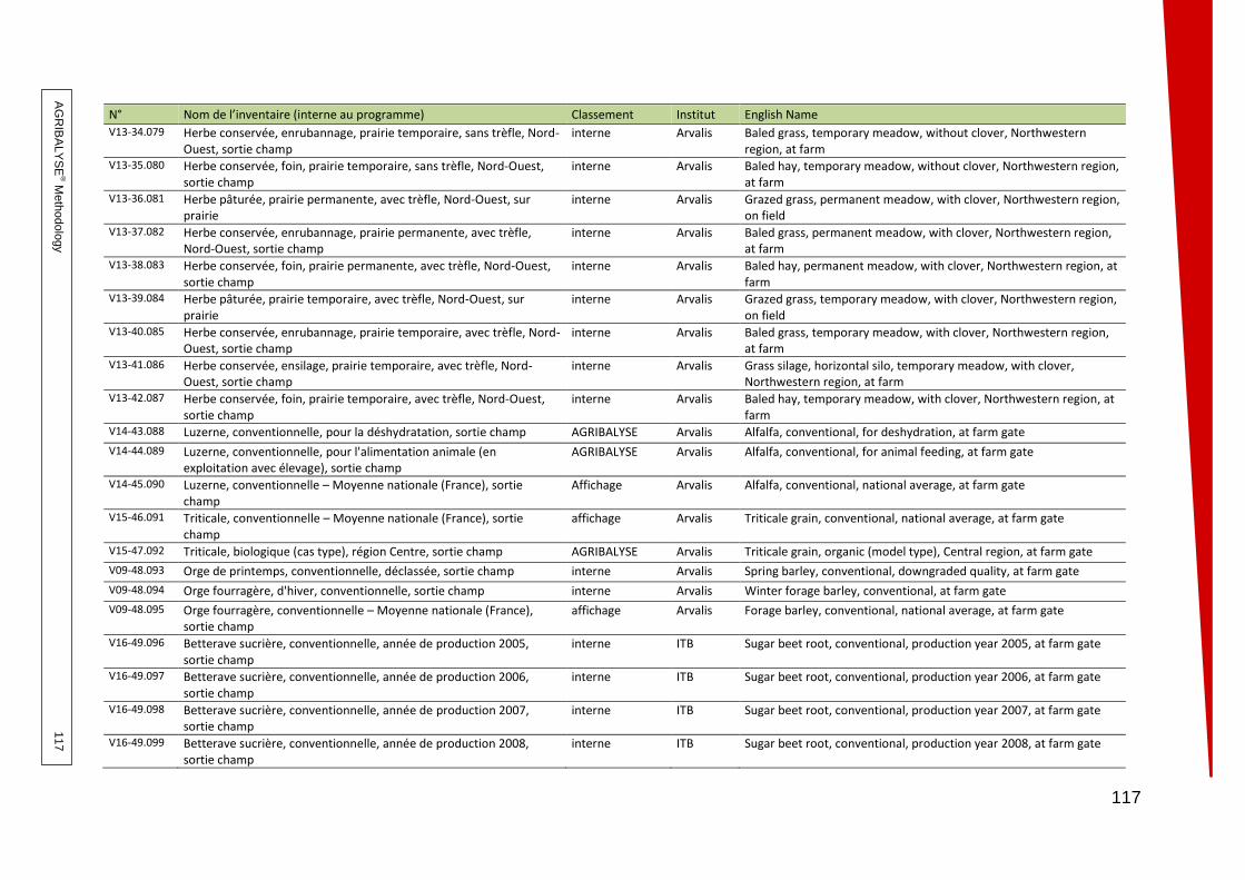
117
AG
RIB
ALY
SE
® Meth
odolo
gy
117
N° Nom de l’inventaire (interne au programme) Classement Institut English Name
V13-34.079 Herbe conservée, enrubannage, prairie temporaire, sans trèfle, Nord-Ouest, sortie champ
interne Arvalis Baled grass, temporary meadow, without clover, Northwestern region, at farm
V13-35.080 Herbe conservée, foin, prairie temporaire, sans trèfle, Nord-Ouest, sortie champ
interne Arvalis Baled hay, temporary meadow, without clover, Northwestern region, at farm
V13-36.081 Herbe pâturée, prairie permanente, avec trèfle, Nord-Ouest, sur prairie
interne Arvalis Grazed grass, permanent meadow, with clover, Northwestern region, on field
V13-37.082 Herbe conservée, enrubannage, prairie permanente, avec trèfle, Nord-Ouest, sortie champ
interne Arvalis Baled grass, permanent meadow, with clover, Northwestern region, at farm
V13-38.083 Herbe conservée, foin, prairie permanente, avec trèfle, Nord-Ouest, sortie champ
interne Arvalis Baled hay, permanent meadow, with clover, Northwestern region, at farm
V13-39.084 Herbe pâturée, prairie temporaire, avec trèfle, Nord-Ouest, sur prairie
interne Arvalis Grazed grass, temporary meadow, with clover, Northwestern region, on field
V13-40.085 Herbe conservée, enrubannage, prairie temporaire, avec trèfle, Nord-Ouest, sortie champ
interne Arvalis Baled grass, temporary meadow, with clover, Northwestern region, at farm
V13-41.086 Herbe conservée, ensilage, prairie temporaire, avec trèfle, Nord-Ouest, sortie champ
interne Arvalis Grass silage, horizontal silo, temporary meadow, with clover, Northwestern region, at farm
V13-42.087 Herbe conservée, foin, prairie temporaire, avec trèfle, Nord-Ouest, sortie champ
interne Arvalis Baled hay, temporary meadow, with clover, Northwestern region, at farm
V14-43.088 Luzerne, conventionnelle, pour la déshydratation, sortie champ AGRIBALYSE Arvalis Alfalfa, conventional, for deshydration, at farm gate
V14-44.089 Luzerne, conventionnelle, pour l'alimentation animale (en exploitation avec élevage), sortie champ
AGRIBALYSE Arvalis Alfalfa, conventional, for animal feeding, at farm gate
V14-45.090 Luzerne, conventionnelle – Moyenne nationale (France), sortie champ
Affichage Arvalis Alfalfa, conventional, national average, at farm gate
V15-46.091 Triticale, conventionnelle – Moyenne nationale (France), sortie champ
affichage Arvalis Triticale grain, conventional, national average, at farm gate
V15-47.092 Triticale, biologique (cas type), région Centre, sortie champ AGRIBALYSE Arvalis Triticale grain, organic (model type), Central region, at farm gate
V09-48.093 Orge de printemps, conventionnelle, déclassée, sortie champ interne Arvalis Spring barley, conventional, downgraded quality, at farm gate
V09-48.094 Orge fourragère, d'hiver, conventionnelle, sortie champ interne Arvalis Winter forage barley, conventional, at farm gate
V09-48.095 Orge fourragère, conventionnelle – Moyenne nationale (France), sortie champ
affichage Arvalis Forage barley, conventional, national average, at farm gate
V16-49.096 Betterave sucrière, conventionnelle, année de production 2005, sortie champ
interne ITB Sugar beet root, conventional, production year 2005, at farm gate
V16-49.097 Betterave sucrière, conventionnelle, année de production 2006, sortie champ
interne ITB Sugar beet root, conventional, production year 2006, at farm gate
V16-49.098 Betterave sucrière, conventionnelle, année de production 2007, sortie champ
interne ITB Sugar beet root, conventional, production year 2007, at farm gate
V16-49.099 Betterave sucrière, conventionnelle, année de production 2008, sortie champ
interne ITB Sugar beet root, conventional, production year 2008, at farm gate

118
AG
RIB
ALY
SE
® Meth
odolo
gy
118
N° Nom de l’inventaire (interne au programme) Classement Institut English Name
V16-49.100 Betterave sucrière, conventionnelle, année de production 2009, sortie champ
interne ITB Sugar beet root, conventional, production year 2009, at farm gate
V16-49.101 Betterave sucrière, conventionnelle – Moyenne nationale (France), sortie champ
affichage ITB Sugar beet roots, conventional, national average, at farm gate
V17-50.102* Pomme à cidre, pépinière, conventionnelle sortie pépinière AGRIBALYSE Astredhor Cider apple, tree seedling, conventional (phase), at tree nursery
V17-50.103* Pomme à cidre, plantation et arrachage, conventionnelle (phase), sortie verger
AGRIBALYSE Astredhor Cider apple, plantation and destruction, conventional (phase), at orchard
V17-50.104* Pomme à cidre, années sans production, conventionnelle (phase), sortie verger
AGRIBALYSE Astredhor Cider apple, period without yield, conventional (phase), at orchard
V17-50.105* Pomme à cidre, années de basse production, conventionnelle (phase), sortie verger
AGRIBALYSE Astredhor Cider apple, low yield production period, conventional (phase), at orchard
V17-50.106* Pomme à cidre, années de pleine production, conventionnelle (phase), sortie verger
AGRIBALYSE Astredhor Cider apple, full production period, conventional (phase), at orchard
V17-50.107 Pomme à cidre, conventionnelle – Moyenne nationale (France), sortie verger
affichage Astredhor Cider apple, conventional, national average, at orchard
V18-51.109 Rose fleur coupée hors sol, lutte intégrée et chauffage faible, sortie serre
AGRIBALYSE Astredhor Rose (cut flower), soilless, low-heated, integrated pest management, at greenhouse
V18-51.110 Rose fleur coupée hors sol, lutte intégrée, chauffée (et éclairée), sortie serre
AGRIBALYSE Astredhor Rose (cut flower), soilless, heated and enlighted, integrated pest management, at greenhouse
V18-51.111 Rose fleur coupée hors sol, lutte conventionnelle et chauffage faible, sortie serre
AGRIBALYSE Astredhor Rose (cut flower), soilless, low-heated, conventional pest management, at greenhouse
V18-51.112 Rose fleur coupée hors sol, lutte conventionnelle, chauffée (et éclairée), sortie serre
AGRIBALYSE Astredhor Rose (cut flower), soilless, heated and enlighted, conventional pest management, at greenhouse
V18-51.113 Rose fleur coupée hors sol, mix de production (lutte conventionnelle et intégrée) – Moyenne nationale (France), sortie serre
affichage Astredhor Rose (cut flower), production mix, national average, at greenhouse
V19-52.115* Arbuste en conteneur, période de production à forte densité (phase), hivernage, sortie serre
AGRIBALYSE Astredhor Potted shrub, wintering (phase), in greenhouse, high density, at production site
V19-52.116* Arbuste en conteneur, période de production à faible densité (phase), extérieur, sortie serre
AGRIBALYSE Astredhor Potted shrub, growing period (phase), outdoor phase, low density, at production site
V19-52.117 Arbuste en conteneur – Moyenne nationale (France), sortie serre affichage Astredhor Potted shrub, national average, at production site
V20-63.128 Féverole, conventionnelle – Moyenne nationale (France), sortie champ
affichage TERRES INOVIA
Faba beans, conventional, national average, at farm gate
V20-64.129 Féverole, de printemps, conventionnelle, en conduite allégée, sortie champ
AGRIBALYSE TERRES INOVIA
Spring faba beans, conventional, reduced protection, at farm gate
V20-65.130 Féverole, biologique en culture pure (cas type), région Centre, sortie champ
AGRIBALYSE TERRES INOVIA
Faba beans, organic (model type), Central Region, at farm gate
V21-66.131 Pois d'hiver, conventionnel, 15% humidité, sortie champ AGRIBALYSE TERRES INOVIA
Winter pea, conventional, 15% moisture, at farm gate

119
AG
RIB
ALY
SE
® Meth
odolo
gy
119
N° Nom de l’inventaire (interne au programme) Classement Institut English Name
V21-67.132 Pois de printemps, conventionnel, 15% humidité, sortie champ AGRIBALYSE TERRES INOVIA
Spring pea, conventional, 15% moisture, at farm gate
V21-68.133 Pois, moyenne nationale (identique avec pois de printemps, V25-67.132)
affichage TERRES INOVIA
(identique avec spring pea)
V22-53-134* Plants de vigne, pépinière production plants greffés soudés (phase), site expérimental tous cépages confondus, sortie champ
AGRIBALYSE IFV Grafted vine plant, nursery, production and varieties mix, at tree nursery
V22-53-135* Plants de vigne, plantation/arrachage conventionnel en Beaujolais Sud (phase), tous vins confondus, sortie champ
AGRIBALYSE IFV Grafted vine, plantation/destruction (phase), conventional, variety mix, Beaujolais, at vineyard
V22-53-136* Plants de vigne, plantation/arrachage conventionnel en Languedoc Roussillon (phase), tous vins confondus, sortie champ
AGRIBALYSE IFV Grafted vine, plantation/destruction (phase), conventional, variety mix, Languedoc-Roussillon, at vineyard
V22-53-137* Raisin, début de production (phase), raisonnée, Beaujolais Sud, vin appellation Beaujolais, sortie champ
AGRIBALYSE IFV Grape, early production (phase), integrated, AOC, Beaujolais, at vineyard
V22-53-138* Raisin, début de production (phase), raisonnée, Languedoc Roussillon, tous vins confondus, sortie champ
AGRIBALYSE IFV Grape, early production (phase), integrated, variety mix, Languedoc-Roussillon, at vineyard
V22-53-139* Raisin, début de production (phase), biologique, Maconnais, vin appellation, sortie champ
AGRIBALYSE IFV Grape, early production (phase), organic, AOC, Maconnais, at vineyard
V22-53-140* Raisin, début de production (phase), biologique, Languedoc Roussillon, tous vins confondus, sortie champ
AGRIBALYSE IFV Grape, early production (phase), organic, variety mix, Languedoc-Roussillon, at vineyard
V22-53-141* Raisin, pleine production (phase), raisonnée, Beaujolais Sud, vin appellation Beaujolais, sortie champ
AGRIBALYSE IFV Grape, full production (phase), integrated, AOC, Beaujolais, at vineyard
V22-53-142* Raisin, pleine production (phase), raisonnée, Languedoc Roussillon, tous vins confondus, sortie champ
AGRIBALYSE IFV Grape, full production (phase), integrated, variety mix, Languedoc-Roussillon, at vineyard
V22-53-143* Raisin, pleine production, biologique (phase), Maconnais, vin appellation, sortie champ
AGRIBALYSE IFV Grape, full production (phase), organic, AOC, Maconnais, at vineyard
V22-53-144* Raisin, pleine production (phase), biologique, Languedoc Roussillon, tous vins confondus, sortie champ
AGRIBALYSE IFV Grape, full production (phase), organic, variety mix, Languedoc-Roussillon, at vineyard
V22-53-145 Raisin vigne, raisonnée, Beaujolais Sud, vin appellation Beaujolais, sortie champ
AGRIBALYSE IFV Grape, integrated, AOC, Beaujolais, at vineyard
V22-53-146 Raisin vigne, raisonnée, Languedoc Roussillon, tous vins confondus, sortie champ
AGRIBALYSE IFV Grape, integrated, variety mix, Languedoc-Roussillon, at vineyard
V22-53-147 Raisin vigne, biologique, Maconnais, vin appellation, sortie champ AGRIBALYSE IFV Grape, organic, AOC, Maconnais, at vineyard
V22-53-148 Raisin vigne, biologique, Languedoc Roussillon, tous vins confondus, sortie champ
AGRIBALYSE IFV Grape, organic, variety mix, Languedoc-Roussillon, at vineyard

120
AG
RIB
ALY
SE
® Meth
odolo
gy
120
TROPICAL PRODUCTS Nb de groupe de produits : 6 Nb Déclinaisons /produits : 6 Nb totale des inventaires (y inclus les inventaires internes et les phases) : 27 Un astérisque indique que c’est un inventaire Phase de production.
N° Nom Produit (interne au programme) Classement Institut English Name
T01-01.001 Riz jasmin, Nord-Est, système pluviale sans irrigation artificielle, sortie champ
interne CIRAD Jasmine rice, North East, Rainfed, Wet season, at farm gate
T01-01.002 Riz jasmin, Nord-Est, système pluviale avec irrigation artificielle, sortie champ
interne CIRAD Jasmine rice, North East, Irrigated, Wet season, at farm gate
T01-01.003 Riz jasmin, Nord-Est, système avec irrigation artificielle, sortie champ interne CIRAD Jasmine rice, North East, Irrigated, Dry season, at farm gate
T01-01.004 Riz jasmin, Nord, système pluviale sans irrigation artificielle, sortie champ
interne CIRAD Jasmine rice, North, Rainfed, Wet season, at farm gate
T01-01.005 Riz jasmin, Nord, système pluviale avec irrigation artificielle, sortie champ
interne CIRAD Jasmine rice, North, Irrigated, Wet season, at farm gate
T01-01.006 Riz jasmin, Nord, système avec irrigation artificielle, sortie champ interne CIRAD Jasmine rice, North, Irrigated, Dry season, at farm gate
T01-01.007 Riz Thaï (Riz jasmin), Moyenne nationale (Thaïlande), sortie champ affichage CIRAD Jasmine rice, national average, at farm gate
T02-02.008* Clémentine (Nour), pépinière (phase), Souss, sortie pépinière interne (phase) CIRAD Clementine, tree seedling (phase), Souss, at tree nursery
T02-02.009* Clémentine (Nour), période non productive (années 1 à 3) (phase), Souss, en verger
interne (phase) CIRAD Clementine, non productive period (phase), Souss, at orchard
T02-02.010* Clémentine (Nour), début production (années 4 à 8) (phase), Souss, en verger
interne (phase) CIRAD Clementine, first production years (phase), Souss, at orchard
T02-02.011* Clémentine (Nour), pleine production (années 9 à 25) (phase), Souss, en verger
interne (phase) CIRAD Clementine, full production period (phase), Souss, at orchard
T02-02.012 Clémentine (Nour), qualité export, Souss, sortie verger affichage CIRAD Clementine, export quality, Souss, at orchard
T03-03.014* Café (Robusta), plantation année 1 (phase), sortie champ interne (phase) CIRAD Coffee bean (Robusta), first year, plantation (phase), Brazil, at farm gate
T03-03.015* Café (Robusta), plantation année 2 (phase), sortie champ interne (phase) CIRAD Coffee bean (Robusta), second year (phase), Brazil, at farm gate
T03-03.016* Café (Robusta), plantation année 3 (phase), sortie champ interne (phase) CIRAD Coffee bean (Robusta), third year (phase), Brazil, at farm gate
T03-03.017* Café (Robusta), sans pulpe, plantation année 4-25 (phase), sortie champ
interne (phase) CIRAD Coffee bean (Robusta), depulped, full production period year (phase), Brazil, at farm gate
T03-03.018 Café du Brésil (Robusta), sans pulpe, Brésil, sortie champ affichage CIRAD Coffee bean (Robusta), depulped, Brazil, at farm gate
T04-04.019* Mangue, période non productive (années 1 à 3) (phase), en verger interne (phase) CIRAD Mango, non productive period (phase), conventional, Brazil, at orchard
T04-04.020* Mangue, début production (années 4 à 10) (phase), en verger interne (phase) CIRAD Mango, first production years (phase), conventional, Brazil, at orchard

121
AG
RIB
ALY
SE
® Meth
odolo
gy
121
N° Nom Produit (interne au programme) Classement Institut English Name
T04-04.021* Mangue, pleine production (années 11 à 25) (phase), en verger interne (phase) CIRAD Mango, full production years (phase), conventional, Brazil, at orchard
T04-04.022 Mangue, conventionnelle, Val de San Francisco, Brésil, sortie verger affichage CIRAD Mango, conventional, Val de San Francisco, Brazil, at orchard
T05-05.023* Cacao pépinière (phase), Brésil, sortie pépinière interne (phase) CIRAD Cocoa tree seedling (phase), Brazil, at tree nursery
T05-05.024* Cacao, période non productive (phase), conventionnel, Cabruca, en verger
interne (phase) CIRAD Cocoa, non productive period (phase), conventional, Cabruca, at orchard
T05-05.025* Cacao, pleine production (phase), conventionnel, Cabruca, en verger interne (phase) CIRAD Cocoa, full production period years (phase), conventional, Cabruca, at orchard
T05-05.026 Cacao, conventionnel, Cabruca, sortie verger affichage CIRAD Cocoa, conventional, Cabruca, at orchard
T06-06.027 Fruit du palmier à huile, conventionnel, Sumatra, , sortie plantation affichage CIRAD Oil palm fruit, conventional, Sumatra, at farm gate

122
AG
RIB
ALY
SE
® Meth
odolo
gy
122
LIVESTOCK PRODUCTION – FRANCE Number of product groups: 19 Number of product variants: 48 N° Nom de l’inventaire Classement Institut English Name
A101-101.101 Lait de vache, conventionnel, système spécialisé de plaine de l’ouest, maïs dominant (>30% maïs / SFP), sortie atelier
AGRIBALYSE IDELE Cow milk, conventional, lowland milk system, silage maize more than 30%, at farm gate
A101-102.102 Lait de vache, conventionnel, système spécialisé de plaine de l’ouest, herbe - maïs (10-30% de maïs / SFP), sortie atelier
AGRIBALYSE IDELE Cow milk, conventional, lowland milk system, silage maize 10 to 30%, at farm gate
A101-103.103 Lait de vache, conventionnel, système spécialisé de plaine, herbe (5 à 10% maïs / SFP), sortie atelier
AGRIBALYSE IDELE Cow milk, conventional, lowland milk system, silage maize 5 to 10%, at farm gate
A101-104.104 Lait de vache, biologique, système spécialisé de plaine de l’ouest, herbe (5 à 10% maïs / SFP), sortie atelier
AGRIBALYSE IDELE Cow milk, organic, lowland milk system, silage maize 5 to 10%, at farm gate
A101-105.105 Lait de vache, conventionnel, système spécialisé de montagne, Massif Central, herbe, sortie atelier
AGRIBALYSE IDELE Cow milk, conventional, highland milk system, grass fed, at farm gate
A101-xxx.106 Lait de vache, Moyenne nationale (France), sortie atelier Affichage IDELE Cow milk, national average, at farm gate
A102-101.107 Vache laitière de réforme, conventionnel, système spécialisé de plaine de l’ouest, maïs dominant (>30% maïs / SFP), sortie atelier
AGRIBALYSE IDELE Cull cow, conventional, lowland milk system, silage maize more than 30%, at farm gate
A102-102.108 Vache laitière de réforme, conventionnel, système spécialisé de plaine de l’ouest, herbe - maïs (10-30% de maïs / SFP), sortie atelier
AGRIBALYSE IDELE Cull cow, conventional, lowland milk system, silage maize 10 to 30%, at farm gate
A102-103.109 Vache laitière de réforme, conventionnel, système spécialisé de plaine, herbe (5 à 10% maïs / SFP), sortie atelier
AGRIBALYSE IDELE Cull cow, conventional, lowland milk system, silage maize 5 to 10%, at farm gate
A102-104.110 Vache laitière de réforme, biologique, spécialisé de plaine de l’ouest, herbe (5 à 10% maïs / SFP), sortie atelier
AGRIBALYSE IDELE Cull cow, organic, lowland milk system, silage maize 5 to 10%, at farm gate
A102-105.111 Vache laitière de réforme, conventionnel, système spécialisé de montagne, Massif Central, herbe, sortie atelier
AGRIBALYSE IDELE Cull cow, conventional, highland milk system, grass fed, at farm gate
A102-106.112 Taurillon laitier, conventionnel, engraisseur spécialisé de taurillons laitiers, sortie atelier
AGRIBALYSE IDELE Young dairy bull, conventional, fattening system, at farm gate
A102-107.113 Vache de réforme d’origine allaitante, conventionnel, naisseur spécialisé, système charolais < 1,2 UGB/ha, sortie atelier
AGRIBALYSE IDELE Suckler cull cow, conventional, suckler cow system, less than 1.2 LU per ha, at farm gate
Product group number A= Livestock production
A02-05.018 Product variant number Data set number

123
AG
RIB
ALY
SE
® Meth
odolo
gy
123
A102-108.114 Génisse race à viande, conventionnel, engraisseur de bœufs ou génisses de race à viande recevant des broutards issus du système naisseur charolais ≥ 1,2 UGB/ha, sortie atelier
AGRIBALYSE IDELE Suckler heifer, conventional, fattening system, more than 1.2 LU per ha, at farm gate
A102-109.115 Taurillon race à viande, conventionnel, engraisseur recevant des broutards issus du système naisseur charolais ≥ 1,2 UGB/ha, sortie atelier
AGRIBALYSE IDELE Young suckler bull, conventional, fattening system, more than 1.2 LU per ha, at farm gate
A102-110.116 Vache de réforme d’origine allaitante, conventionnel, naisseur spécialisé, système charolais ≥ 1,2 UGB/ha, sortie atelier
AGRIBALYSE IDELE Suckler cull cow, conventional, suckler cow system, more than 1.2 LU per ha, at farm gate
A102-111.117 Taurillon race à viande, conventionnel, engraisseur spécialisé recevant des broutards issus du système naisseur charolais < 1,2 UGB/ha, sortie atelier
AGRIBALYSE IDELE Young suckler bull, conventional, fattening system, less than 1.2 LU per ha, at farm gate
A102-xxx.118 Bovin viande, Moyenne nationale (France), sortie atelier Affichage IDELE Beef cattle, national average, at farm gate
A103-112.119 Veau de boucherie, conventionnel, atelier d’engraissement recevant des veaux de 8 jours issus de systèmes laitiers de plaine, sortie atelier
Affichage IDELE Beef calf, conventional, fattening system, calves from lowland milk system, at farm gate
A104-113.120 Lait de brebis, conventionnel, système Roquefort, sortie atelier AGRIBALYSE IDELE Sheep milk, conventional, Roquefort system, at farm gate
A105-114.121 Lait de chèvre, conventionnel, système zone fourragère intensive, centre ouest, sortie atelier
AGRIBALYSE IDELE Goat milk, conventional, intensive forage area, at farm gate
A106-115.122 Agneau, conventionnel, système spécialisé bergerie, sortie atelier Affichage IDELE Lamb, conventional, indoor production system, at farm gate
A107-116.123 Œuf, biologique, sortie atelier (Bretagne) AGRIBALYSE ITAVI Egg, organic, at farm gate
A107-117.124 Œuf, conventionnel, plein air, sortie atelier (Pays de la Loire, Sarthe) AGRIBALYSE ITAVI Egg, conventional, outdoor system, at farm gate
A107-118.125 Œuf, conventionnel, en bâtiment, au sol, sortie atelier (Bretagne) AGRIBALYSE ITAVI Egg, conventional, indoor system, non-cage, at farm gate
A107-119.126 Œuf, conventionnel, en bâtiment, en cage, sortie atelier (Bretagne, Côtes d’Armor) AGRIBALYSE ITAVI Egg, conventional, indoor system, cage, at farm gate
A107-120.127 Œuf, conventionnel, en bâtiment, en cage, réglementation 2012, sortie atelier (Bretagne, Côtes d’Armor)
AGRIBALYSE ITAVI Egg, conventional, indoor production, cage 2012 rules, at farm gate
A107-xxx.128 Œuf, Moyenne nationale (France), sortie atelier Affichage ITAVI Egg, national average, at farm gate
A108-121.129 Poulet de chair, conventionnel, sortie atelier AGRIBALYSE ITAVI Broiler, conventional, at farm gate
A108-122.130 Poulet de chair, Label rouge, sortie atelier AGRIBALYSE ITAVI Broiler, Label Rouge, at farm gate
A108-123.131 Poulet de chair, biologique, sortie atelier AGRIBALYSE ITAVI Broiler, organic, at farm gate
A108-xxx.132 Poulet de chair, Moyenne nationale (France), sortie atelier Affichage ITAVI Broiler, national average, at farm gate
A109-124.133 Dinde, conventionnel, sortie atelier (Bretagne, Morbihan) AGRIBALYSE ITAVI Turkey, conventional, at farm gate

124
AG
RIB
ALY
SE
® Meth
odolo
gy
124
A109-125.134 Dinde, Label rouge, sortie atelier (Bretagne, Morbihan) AGRIBALYSE ITAVI Turkey, Label Rouge, at farm gate
A109-xxx.135 Dinde, Moyenne nationale (France), sortie atelier Affichage ITAVI Turkey, national average, at farm gate
A110-126.136 Palmipède gras , canard à gaver, conventionnel, sortie atelier (Aquitaine, Landes) Affichage ITAVI Fattening duck, conventional, at farm gate
A111-127.137 Canard à rôtir, conventionnel (sur caillebotis), sortie atelier (Pays de la Loire, Vendée) Affichage ITAVI Duck for roasting, conventional, at farm gate
A112-128.138 Truite portion, 250-350g, convenntionel, sortie atelier Affichage ITAVI Small trout, 250-350g, conventional, at farm gate
A113-129.139 Grande truite, 2 à 4kg, conventionnel, sortie atelier Affichage ITAVI Large trout, 2-4kg, conventional, at farm gate
A114-130.140 Bar ou dorade, 200 à 500g, conventionnel, en cage, sortie atelier (méditerranée) Affichage ITAVI Sea bass or sea bream, 200-500g, conventional, in cage, at farm gate
A115-131.141 Lapin, conventionnel, en cage, sortie atelier (Pays de la Loire, Vendée) Affichage ITAVI Rabbit, conventional, in cage, at farm gate
A116-132.142 Porc, conventionnel, alimentation à dominante colza, sortie atelier AGRIBALYSE IFIP Pig, conventional, fed rapeseed meal, at farm gate
A116-133.143 Porc, conventionnel, alimentation à dominante soja, sortie atelier AGRIBALYSE IFIP Pig, conventional, fed soybean meal, at farm gate
A116-134.144 Porc, conventionnel, d'exploitation céréales/porcs en approvisionnement local, sortie atelier (Pays de la Loire)
AGRIBALYSE IFIP Pig, conventional, on-farm feed supply, at farm gate
A116-135.145 Porc, conventionnel, standard d'élevage spécialisé avec traitement biologique des effluents - 100% achat, sortie atelier
AGRIBALYSE IFIP Pig, conventional, excess slurry treatment, at farm gate
A116-136.146 Porc, conventionnel, Moyenne nationale (France), sortie atelier Affichage IFIP Pig, conventional, national average, at farm gate
A117-137.147 Porc, Label Rouge, bâtiment courette, sortie atelier Affichage IFIP Pig, Label Rouge, pig with run system, at farm gate
A117-138.148 Porc, Label Rouge, plein air, sortie atelier Affichage IFIP Pig, Label Rouge, outdoor system, at farm gate
A118-139.149 Porc, biologique, sortie atelier Affichage IFIP Pig, organic, at farm gate
Axxx-101.150 Veau, conventionnel, système spécialisé de plaine de l’ouest, maïs dominant (>30% maïs / SFP), sortie atelier
AGRIBALYSE IDELE Calf, conventional, lowland milk system, silage maize more than 30%, at farm gate
Axxx-102.151 Veau, conventionnel, système spécialisé de plaine de l’ouest, herbe - maïs (10-30% de maïs / SFP), sortie atelier
AGRIBALYSE IDELE Calf, conventional, lowland milk system, silage maize 10 to 30%, at farm gate
Axxx-103.152 Veau, conventionnel, système spécialisé de plaine, herbe (5 à 10% maïs / SFP), sortie atelier
AGRIBALYSE IDELE Calf, conventional, lowland milk system, silage maize 5 to 10%, at farm gate
Axxx-104.153 Veau, biologique, système spécialisé de plaine de l’ouest, herbe (5 à 10% maïs / SFP), sortie atelier
AGRIBALYSE IDELE Calf, organic, lowland milk system, silage maize 5 to 10%, at farm gate
Axxx-105.154 Veau, conventionnel, système spécialisé de montagne, herbe, Massif Central, sortie atelier
AGRIBALYSE IDELE Calf, conventional, highland milk system, grass fed, at farm gate

125
AG
RIB
ALY
SE
® Meth
odolo
gy
125
Axxx-107.154 Broutard, conventionnel, naisseur spécialisé, système charolais < 1,2 UGB/ha, sortie atelier
AGRIBALYSE IDELE Cattle weaner, conventional, suckler cow system, less than 1.2 LU per ha, at farm gate
Axxx-110.156 Broutard, conventionnel, naisseur spécialisé, système charolais ≥ 1,2 UGB/ha, sortie atelier
AGRIBALYSE IDELE Cattle weaner, conventional, suckler cow system, more than 1.2 LU per ha, at farm gate
Axxx-113.157 Brebis laitière de réforme, conventionnel, système Roquefort, sortie atelier Affichage IDELE Cull ewe, conventional, Roquefort system, at farm gate
Axxx-113.158 Agneau, conventionnel, système Roquefort, sortie atelier Affichage IDELE Lamb, conventional, Roquefort system, at farm gate
Axxx-113.159 Laine, conventionnel, système Roquefort, sortie atelier Affichage IDELE Wool, conventional, Roquefort system, at farm gate
Axxx-114.160 Chèvre de réforme, conventionnel, système zone fourragère intensive, centre ouest, sortie atelier
AGRIBALYSE IDELE Cull goat, conventional, intensive forage area, at farm gate
Axxx-114.161 Chevreau, conventionnel, système zone fourragère intensive, centre ouest, sortie atelier
Affichage IDELE Kid goat, conventional, intensive forage area, at farm gate
Axxx-115.162 Brebis allaitante de réforme, conventionnel, système spécialisé bergerie, sortie atelier AGRIBALYSE IDELE Cull ewe, conventional, indoor production system, at farm gate
Axxx-115.163 Laine, conventionnel, système spécialisé bergerie, sortie atelier AGRIBALYSE IDELE Wool, conventional, indoor production system, at farm gate
Axxx-116.164 Poule de réforme, biologique, sortie atelier (Bretagne) AGRIBALYSE ITAVI Cull hen, organic, at farm gate
Axxx-117.165 Poule de réforme, conventionnel, plein air, sortie atelier (Pays de la Loire, Sarthe) AGRIBALYSE ITAVI Cull hen, conventional, outdoor system, at farm gate
Axxx-118.166 Poule de réforme, conventionnel, en bâtiment, au sol, sortie atelier (Bretagne) AGRIBALYSE ITAVI Cull hen, conventional, indoor system, non-cage, at farm gate
Axxx-119.167 Poule de réforme, conventionnel, en bâtiment, en cage, sortie atelier (Bretagne, Côtes d’Armor)
AGRIBALYSE ITAVI Cull hen, conventional, indoor system, cage, at farm gate
Axxx-120.168 Poule de réforme, conventionnel, en bâtiment, en cage, réglementation 2012, sortie atelier (Bretagne, Côtes d’Armor)
AGRIBALYSE ITAVI Cull hen, conventional, indoor production, cage 2012 rules, at farm gate
Axxx-xxx.169 Poule de reforme, Moyenne nationale (France), sortie atelier Affichage ITAVI Cull hen, conventional, national average, at farm gate
Axxx-131.170 Lapine de reforme, conventionnel, en cage, sortie atelier Affichage ITAVI Cull rabbit, conventional, in cage, at farm gate
Axxx-132.171 Truie de reforme, conventionnel, alimentation à dominante colza, sortie atelier AGRIBALYSE IFIP Cull sow, conventional, fed rapeseed meal, at farm gate
Axxx-133.172 Truie de reforme, conventionnel, alimentation à dominante soja, sortie atelier AGRIBALYSE IFIP Cull sow, conventional, fed soybean meal, at farm gate
Axxx-134.173 Truie de reforme, conventionnel, d'exploitation céréales/truies en approvisionnement local, sortie atelier (Pays de la Loire)
AGRIBALYSE IFIP Cull sow, conventional, on-farm feed supply, at farm gate
Axxx-135.174 Truie de réforme, conventionnel, standard d'élevage spécialisé avec traitement biologique des effluents - 100% achat, sortie atelier
AGRIBALYSE IFIP Cull sow, conventional, excess slurry treatment, at farm gate
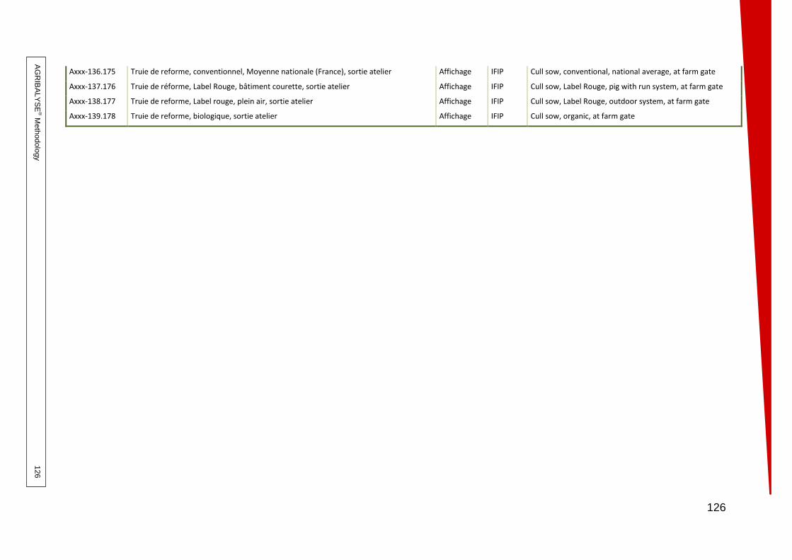
126
AG
RIB
ALY
SE
® Meth
odolo
gy
126
Axxx-136.175 Truie de reforme, conventionnel, Moyenne nationale (France), sortie atelier Affichage IFIP Cull sow, conventional, national average, at farm gate
Axxx-137.176 Truie de réforme, Label Rouge, bâtiment courette, sortie atelier Affichage IFIP Cull sow, Label Rouge, pig with run system, at farm gate
Axxx-138.177 Truie de reforme, Label rouge, plein air, sortie atelier Affichage IFIP Cull sow, Label Rouge, outdoor system, at farm gate
Axxx-139.178 Truie de reforme, biologique, sortie atelier Affichage IFIP Cull sow, organic, at farm gate

AGRIBALYSE®: Methodology 127
Appendix B: Calculating national LCI data sets (French average)
Plant production
1. Carrot, conventional – French Average
Table 38: Composition of the national conventional carrot data set
Data set Weighting in the national LCI data set (%)
Carrot, early, conventional, Aquitaine 27.4
Carrot, main season, conventional, Aquitaine 25.2
Carrot, winter, conventional, Aquitaine 15.4
Carrot, fall, conventional, Créances 7.7
Carrot, winter, conventional, , Créances 11.6
Carrot, fall, conventional, Val de Saire 1.8
Carrot, winter, conventional, Val de Saire 4.1
Carrot, fall, conventional, Mont St Michel 5.4
Carrot, winter, conventional, Mont St Michel 1.4
Data based on expert opinion when collecting data for the carrot data sets for the AGRIBALYSE program. The “Conventional carrot French average for sale as fresh produce” is the weighted mean of the basic data sets listed above. These nine regional data sets are classified “interne” and are not published in the AGRIBALYSE database.
2. Alfalfa, conventional – French Average
Table 39: Composition of the national conventional alfalfa data set
Data set Weighting in the national LCI data set (%)
Alfalfa for dehydration 33
Alfalfa for animal feeding 77
Data based on expert opinion when collecting data for the alfalfa data sets for the AGRIBALYSE program. The “Conventional alfalfa French average” is the weighted mean of the two basic data sets listed above.
3. Conventional barley, malting quality – French Average Table 40: Composition of the national data set for malting quality barley
Data set Weighting in the national LCI data set (%)
Spring barley, conventional, malting quality 54
Winter barley, conventional, malting quality 46
Data based on expert opinion when collecting data for the barley data sets for the AGRIBALYSE program. The “Conventional malting quality barley French average” is the weighted mean of the two basic data sets listed above. These two data sets are classified “interne” and are not published in the AGRIBALYSE database.

AGRIBALYSE®: Methodology 128
4. Forage barley, conventional – French Average Table 41: Composition of the national forage barley dataset
Data set Weighting in the national LCI data set (%)
Spring barley, conventional, downgraded quality 15
Winter forage barley, conventional 66
Winter barley, conventional, malting quality 19
Data based on expert opinion when collecting data for the barley data sets for the AGRIBALYSE program. The “Conventional forage barley French Average” data set is the weighted mean of the basic data sets listed above. These nine regional data sets are classified “interne” and are not published in the AGRIBALYSE database.
5. Peaches/nectarines – French average Table 42: Composition of the national peach/nectarine data set
Data set Weighting in the national LCI data set (%)
Peach/nectarine, conventional – French average 98.5
Peach/nectarine, organic – French average 1.5
Data based on expert opinion when collecting data for the peach/nectarine data sets for the AGRIBALYSE program. The “Peach/nectarine French average” data set is the weighted mean of the basic data sets listed above. The two data sets are based on several growth phase data sets which are published in the AGRIBALYSE database.
6. Eating apples, conventional – French average
Table 43: Composition of the national conventional eating apple data set (scab-resistant and non scab-resistant varieties)
Data set Weighting in the national LCI data set (%)
Apple non-scab resistant, conventional – French average
90
Apple scab resistant, conventional – French average 10
Data based on expert opinion when collecting data for the apple data sets for the AGRIBALYSE program. The “Conventional eating apple French average” data set is the weighted mean of the two basic data sets listed above. The two data sets are based on several growth phase data sets which are published in the AGRIBALYSE database.
1. Eating apples – French average Table 44: Composition of the national eating apple data set
Data set Weighting in the national LCI data set (%)
Eating apple, conventional – French average 98.5
Eating apple, organic – French average 1.5

AGRIBALYSE®: Methodology 129
Data based on expert opinion when collecting data for the apple data sets for the AGRIBALYSE program. The Eating apple French average data set data set is the weighted mean of the two basic data sets listed above.
2. Potato, conventional – French average Table 45: Composition of the national potato dataset
Data set Weighting in the national LCI data set (%)
Starch potato, conventional – French average 20
Potato for industrial use, conventional 28
Potato for fresh market, other varieties, conventional 52
Data based on expert opinion when collecting data for the potato data sets for the AGRIBALYSE program. The Potato French average data set is the weighted mean of the basic data sets listed above.
3. Rose (cut flower), soilless – French average Table 46: Composition of the national rose (cut flower) soilless data set
Data set Weighting in the national LCI data set (%)
Rose (cut flower) soilless, integrated pest management with low heating
12
Rose (cut flower) soilless, integrated pest management, with heating and lighting
53
Rose (cut flower) soilless, conventional pest management, with low heating
19
Rose (cut flower) soilless, conventional pest management, with heating and lighting
16
Data based on expert opinion when collecting data for the rose data sets for the AGRIBALYSE program. The Rose (cut flower) soilless, French average data set is the weighted mean of the basic data sets listed above.
4. Thai rice (Jasmine rice) – Thai average Table 47: Composition of the national Thai rice data set
Data set Weighting in the national LCI data set (%)
Thai rice (jasmine rice) North East, Rainfed, Wet Season 66.2
Thai rice (jasmine rice) North East, Irrigated, Wet Season 11.8
Thai rice (jasmine rice) North East, Irrigated, Dry Season 5.9
Thai rice (jasmine rice) North, Rainfed, Wet Season 1.9
Thai rice (jasmine rice) North, Irrigated, Wet Season 7.1
Thai rice (jasmine rice) North, Irrigated, Dry Season 7.1
Data from the national Thai rice production statistics. The “Thai rice, Thai average” data set is the weighted mean of the basic data sets listed above. These seven regional data sets are classified “interne” and are not published in the AGRIBALYSE database.

AGRIBALYSE®: Methodology 130
5. Tomato for the fresh market, conventional, greenhouse production – French average
Table 48: Composition of the national conventional tomato greenhouse production for the fresh market data set
Data set Weighting in the national LCI data set (%)
Tomato for the fresh market, conventional, unheated greenhouse production - French average
13.7
Tomato for the fresh market, conventional, heated greenhouse production– French average
86.3
Data based on expert opinion when collecting data for the tomato data sets for the AGRIBALYSE program. The Tomato for the fresh market, conventional, greenhouse production data set is the weighted mean of the two basic data sets listed above. As the “Tomato, conventional, French average, heated greenhouse production” data set is classified “interne” it is not published in the AGRIBALYSE database.
6. Tomato for the fresh market, greenhouse production – French average Table 49: Composition of the national tomato for the fresh market data set
Data set Weighting in the national LCI data set (%)
Tomato for the fresh market, conventional, unheated greenhouse production - French average
13,5
Tomato for the fresh market, conventional, heated greenhouse production - French average
85
Tomato for the fresh market, organic, greenhouse production - French average
1,5
Data based on expert opinion while collecting data for the tomato data sets for the AGRIBALYSE program. The “Tomato for the fresh market French average” data set is the weighted mean of the basic data sets listed above. As the “Tomato conventional French average heated greenhouse production” data set is classified “interne” it is not published in the AGRIBALYSE database.
7. Sugar beet, conventional – French average Table 50: Composition of the national conventional sugar beet data set
Data set Weighting in the national LCI data set (%)
Sugar beet, conventional, production year 2005
20
Sugar beet, conventional, production 2006 20
Sugar beet, conventional, production 2007 20
Sugar beet, conventional, production 2008 20
Sugar beet, conventional, production 2009 20
Data based on national statistics (Agreste 2009). The “Sugar beet conventional French average” data set is the weighted mean of the basic data sets listed above. These five data sets are classified “interne” and are not published in the AGRIBALYSE database;

AG
RIB
ALY
SE
®: Meth
odolo
gy
131
Livestock production Table 51: Composition of the national cow’s milk LCI data set
AGRIBALYSE Classification Study by the Institut de l'Elevage Observatoire de l'Alimentation des Vaches
Laitières, 2011 % of the
AGRIBALYSE milk
average Data set Classification System
N° System name
Number of farms
Standard quantity of milk / farm
Total qty of system =
number of farms x Qty
milk per farm
% of total national
production
Cow’s milk, conventional, lowland milk system, maize dominant (maize more than 30%), at farm gate AGRIBALYSE 2
Specialist lowland >
30% w 9226 307 983 2 841 451 158 12.3% 58.2%
Cow’s milk, conventional, lowland milk system, grass- maize (maize 10 to 30% ), at farm gate AGRIBALYSE 4
Specialist lowland 10-
30% w 3536 251 236 888 370 496 3.8% 18.2%
Cow’s milk, conventional, lowland milk system, silage maize 5 to 10%, at farm gate
AGRIBALYSE
5 Specialist lowland
<10% 2615 200 801 525 094 615 2.3% 10.8%
Cow’s milk, organic, lowland milk system, silage maize 5 to 10% , at farm gate
AGRIBALYSE
Cow’s milk, conventional, highland milk system, Massif Central, grass fed, at farm gate AGRIBALYSE 8
Mountain grass – Massif Central
4003 156 694 627 246 082 2.7% 12.8%
Cow’s milk, French average, at farm gate Affichage (labeling) TOTAL 21.1% 100.0%

AG
RIB
ALY
SE
®: Meth
odolo
gy
132
Table 52: Composition of national beef cattle LCI data set
AGRIBALYSE Classification
Description
Proportion of meat production in France (large cattle)
% of AGRIBALYSE beef average Data set Classification
Key figures for 2010–Institut de l’Elevage,
GEB
Extrapolation
Cull cow, conventional, lowland milk system, silage maize more than 30% at farm gate
AGRIBALYSE
Cow - dairy 26%
26%*58,2% =15.132
16.81%
Cull cow, conventional, lowland milk system, silage maize 10-30% at farm gate AGRIBALYSE
26%*18.2% =4.732%
5.25%
Cull cow, conventional and organic, lowland milk system, grass, at farm gate AGRIBALYSE
26%*10.8% = 2.808%
3.12%
Cull cow, conventional , highland milk system, Massif Central, grass, at farm gate AGRIBALYSE
26%*12.8%= 3.328%
3.69%
Young dairy bull, conventional, fattening system, at farm gate AGRIBALYSE
Young bull -dairy
8% 8% 8.88%
Suckler cull cow, conventional, suckler cow system, less than 1.2 LU/ha, at farm gate AGRIBALYSE
Cow - suckler
22%
22%*50% = 11%
12.22%
Suckler cull cow, conventional, suckler cow system, more than 1.2 LU/ha, at farm gate AGRIBALYSE
22%*50% = 11%
12.22%
Suckler heifer, conventional, fattening system. more than 1.2 LU/ha, at farm gate AGRIBALYSE
Heifer -suckler
10% 10% 11.11%
Young suckler bull, conventional, fattening system, more than 1.2 LU/ha, at farm gate AGRIBALYSE
Young bull -suckler
24%
24%*50% = 12%
13.33%
Young suckler bull, conventional, fattening system, less than 1.2 LU/ha, at farm gate
AGRIBALYSE 24%*50% =
12% 13.33%
Beef cattle, French average, at farm gate affichage 90% 100%

AGRIBALYSE®: Methodology 133
Table 53: Composition of national average egg LCI data set
Data set Weighting in the national LCI data set (%)
Eggs, indoor system, cage 83
Eggs, indoor system, non cage 4.5
Eggs, outdoor system 9.5
Eggs, organic 3
Data taken from the AGRESTE poultry survey (2008). The “Egg French average” data set is the weighted mean of the basic data sets listed above. Table 54: Composition of the national average broiler data set
Data set Weighting in the national LCI data set (%)
Broiler, conventional 87.5
Broiler, Label Rouge 12
Broiler, organic 0.5
Data taken from the AGRESTE poultry survey (2008). The “Broiler French average” data set is the weighted mean of the basic data sets listed above. Table 55: Composition of the national average turkey data set
Data set Weighting in the national LCI data set (%)
Turkey, conventional 97
Turkey, Label Rouge 3
Data taken from the AGRESTE poultry survey AGRESTE (2008). The “Turkey French average” data set is the weighted mean of the basic data sets listed above.

AGRIBALYSE®: Methodology 134
Appendix C: Specification for quality control of production system data
collected for the AGRIBALYSE program

AGRIBALYSE June 2011
For AGRIBALYSE quality control
experts
Authors
Peter Koch
Thibault Salou
Quality control of French production system data
Specification
VERSION 1.0

AGRIBALYSE Program
Specification: Quality control of French production system data Version 4, June 2011

1 Introduction – Purpose of the specification
This specification is intended to provide answers to questions on the methodology and practices that might be raised by the experts selected for the quality control phase of the data collected for the production systems describing the farming production processed in the AGRIBALYSE program. Its aim is to: i) help the experts carry out their quality control brief and ii) harmonize the data quality assessments produced by the various experts. To achieve these aims, this specification defines:
The scope of the data subject to quality control The assessment methods
Partners of the AGRIBALYSE program

2 Presentation of the quality control procedure for the
AGRIBALYSE program The credibility of the database built for the AGRIBALYSE program relies on strict quality control. There are three stages in the quality control process:
1. Verification, by the project leaders, of the data and information entered by the
Technical Institutes
2. Quality control of the data describing the production systems of the French
production process, carried out by organizations external to the program
3. Quality control of the LCI and LCIA results, undertaken by the Technical Institutes
supporting the program
A working seminar will be organized at the end of the second and third phases. This document concerns the second quality control phase. This phase is divided into two stages. The first stage is quality control by the experts and the second stage is the assessment of their comments on checking the data at seminar N°3 (February 2012). This seminar will decide what action, if any, should be taken on the comments from the experts. The experts are invited to attend the seminar but this is not compulsory.
3 Quality control framework For the AGRIBALYSE program, it was decided that each expert should check a group of similar agricultural production processes (eg all oleaginous plants), depending on his field of competence.
3.1 Scope of quality control
Comment The AGRIBALYSE program was set up to build a database of LCI datasets for French agricultural production. The data was, therefore, collected for “French average” production, in most cases. One of the aims of the program is to ensure that the various products were handled uniformly. These two requirements require a strict definition of the methodology to be used (system boundaries, functional units, allocation, etc.). The quality control required here does not cover the methodological choices. Experts are required to check:
a) Compliance with the main recommendations defined in the Data Collection Guide for the AGRIBALYSE program
b) Data for French production systems As most of the data is for “French average” production systems, experts are not required to give their opinion on the precision of the data entered for particular situations. They are asked to give their opinion on the plausibility of the data entered.

They are asked to fill in the “Evaluation” column on the forms with the following scores:
Plausible data: the data entered conforms, in the AGRIBALYSE context, to current French agricultural production practices
With reservations: the values entered are borderline for what is usually found but remain plausible. If possible, they should be verified to check that there are no errors. This score should be supported by a comment.
Unacceptable : the values are unrealistic or suspect and need to be corrected. This score should be supported by a comment.
No opinion: if the expert was not qualified to evaluate the data quality Experts are also asked to comment on any omissions or incoherences in the data checked. Note: Depending on his conclusion (“major modifications required, to be reviewed after modifications”), the expert may be asked to carry out a second review to verify the quality of the data that has been modified.
3.2 General section
The first part covers general points common to the livestock and plant production processes. The following points are evaluated. (A) Correspondence between the name of the process and its content
Does the name of the process correspond to the content?
Is the name sufficiently explicit? (B) Implementation of the principles in the Data Collection Guide
Are the main recommendations set out in the Data Collection Guide correctly applied?
(C) Data quality: - Representativeness
Technological
Geographical
Time-related: is the data representative of the reference period (2005-2009)? (D) Documentation
Are the data and calculations adequately documented?
Are the documents cited available to the public?
3.3 Livestock production
The data to be checked is divided into various groups (see livestock production form). Different information is evaluated for each group.
Activity data
Yields: weight of animals on output, quantities produced (eggs/milk)
Time spent on the farm

Specific technical data (eg: lean meat percentage for pigs)
Feed
This section has two parts, one for the formulation of feed mixes and one defining the composition of rations. The following data should to be checked:
Formulation of the feed mixes: list of raw materials and proportions
Composition of the rations
Distribution of rations for a given class of animals
Excretions
Management in buildings, quantities, dry matter content, storage duration
Management during storage: storage structure, duration, quantities managed
Dates
Distribution of feed rations
Turning ruminants out to grass
Buildings
Type, area
Time spent by animals in buildings
Power consumption
Fossil fuel (natural gas, propane/butane, oil, electricity)
Lubricants
3.4 Arable / horticultural production
The data to be checked is divided into various groups (see plant production form). Different information is evaluated for each group. Yield and co-products
Yield: suitability of the functional unit definition (in particular details of the product quality), quantities produced and variations.
Permanent crops: duration of the process
Co-products: quantities produced
Plausibility of the yield of the main product
Management of intercrops
Previous crop: date of harvest, distribution and quantity of crop residues
Plausibility of the intercrop management (no intermediate crop, intermediate crop not sold, with intermediate crop sold)
Tilling and drilling (quantities and mechanization)
Suitability of the production system for tilling
Quantities of seed sown and proportion of farm seed

Fertilization (quantities and mechanization)
Plausibility of fertilizers used
Application methods (mechanization) and frequency (number of passes)
Plausibility of quantities applied (and variation)
Pesticides (quantities and mechanization)
Plausibility of active substances used
Application methods (mechanization) and frequency (number of passes)
Plausibility of quantities applied (and variation) Sundry
Irrigation (if appropriate): volume of water used for watering, amount of power used and type of power
Suitability of the various inputs entered
Travel of seasonal labor: distances and number of seasonal workers per data collection unit
Plausibility of the dates
Dates for harvesting previous crops
Dates for tilling
Date for sowing main crop
Dates of fertilization (if given)
Dates for applying pesticides (if given)
Date for harvesting main crop
3.5 Estimated time taken for each process
Estimated workload for each process 1. Evaluation of the specific criteria: 2 to 5 minutes for each section 10 – 35 minutes 2. Filling in the review form: 30 – 45 minutes
For each process 40 – 80 minutes It is likely that the speed of evaluation will improve. The upper limit applies, therefore, to the first processes checked.
3.6 Reporting
The review forms should be returned to the project leaders. One review form should be returned for each production system reviewed.
4 Documents provided Various documents are provided for the experts to make it easier to check the quality of the production system data.

4.1 Specification
This document. It provides the information required on the quality control aims and methods. It defines the quality control procedures: what data should be checked and how this should be done. The specification also includes important information on the schedule, confidentiality, etc.
4.2 Production system data
When the expert has signed a confidentiality agreement, production system data will be sent in the form of EXCEL spreadsheets. These were prepared by the project leaders and extracted from the data collection module. They contain all the data to be checked.
4.3 Review forms
The review forms are designed i) to provide a checklist for the data to make it easier to check the data ii) to ensure that the data review is consistent. These review forms should be sent back to the project leaders. One form should be filled in for each process checked. The review forms have a formal part setting out the criteria to be evaluated. This part is the core element of the review process and should be filled in. The second part allows experts greater freedom to give a more general assessment of the quality of the data checked.
4.4 Main recommendations in the Data Collection Guide
An overview of the main recommendations in the Data Collection Guide for the AGRIBALYSE program is provided for the experts to make it easier for them to check that the data entered complies with these recommendations.
4.5 Confidentiality agreement
The confidentiality agreement ensures that the data sent for quality control will be kept confidential. This agreement must be signed before the start of the quality control procedure.
5 Schedule The quality control procedure is scheduled to take place during fall 2011 and the phase for checking French production system data is scheduled to end with a working seminar in

February 2012. To make preparations for this phase, experts are asked to send their reports to the appropriate project leaders within at least four weeks after receiving the data to be checked.
6 Confidentiality Experts are reminded that the data sent is confidential and must be treated as such. It may not be used outside the scope of the AGRIBALYSE program.
7 Main recommendations in the Data Collection Guide Table 56 below lists the main recommendations to ensure that the data collected for the AGRIBALYSE program is consistent.
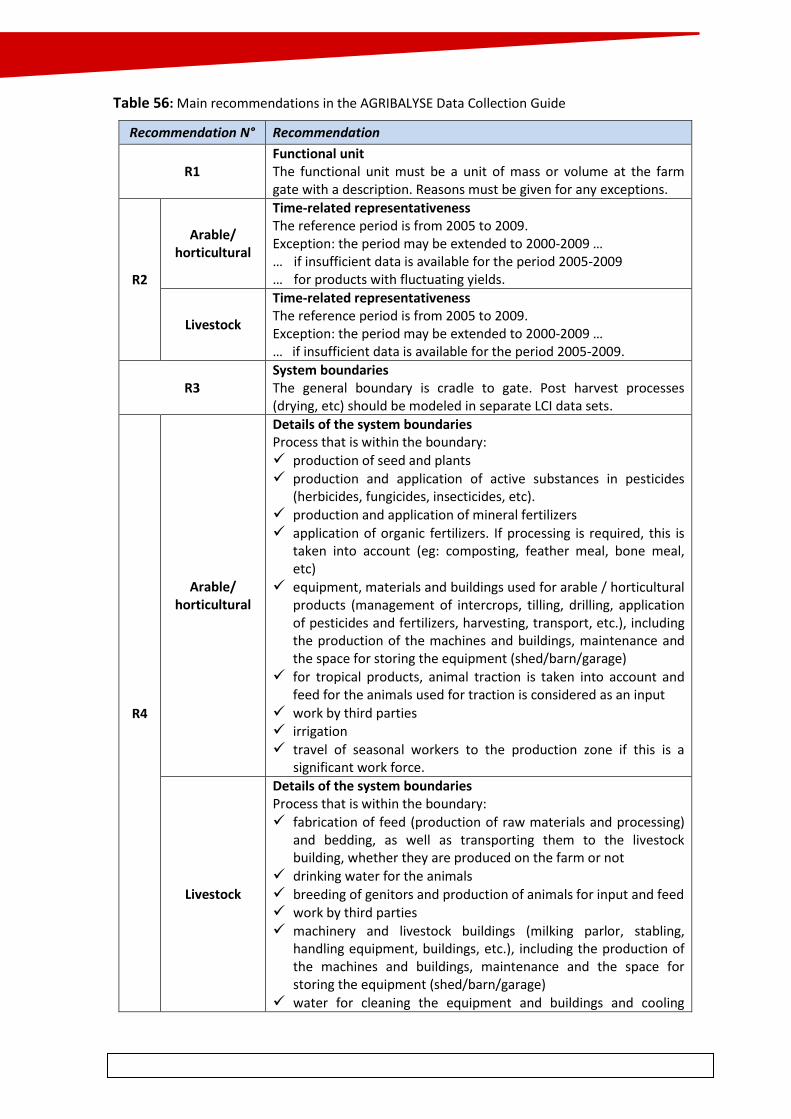
Table 56: Main recommendations in the AGRIBALYSE Data Collection Guide
Recommendation N° Recommendation
R1 Functional unit The functional unit must be a unit of mass or volume at the farm gate with a description. Reasons must be given for any exceptions.
R2
Arable/ horticultural
Time-related representativeness The reference period is from 2005 to 2009. Exception: the period may be extended to 2000-2009 … … if insufficient data is available for the period 2005-2009 … for products with fluctuating yields.
Livestock
Time-related representativeness The reference period is from 2005 to 2009. Exception: the period may be extended to 2000-2009 … … if insufficient data is available for the period 2005-2009.
R3 System boundaries The general boundary is cradle to gate. Post harvest processes (drying, etc) should be modeled in separate LCI data sets.
R4
Arable/ horticultural
Details of the system boundaries Process that is within the boundary: production of seed and plants production and application of active substances in pesticides
(herbicides, fungicides, insecticides, etc). production and application of mineral fertilizers application of organic fertilizers. If processing is required, this is
taken into account (eg: composting, feather meal, bone meal, etc)
equipment, materials and buildings used for arable / horticultural products (management of intercrops, tilling, drilling, application of pesticides and fertilizers, harvesting, transport, etc.), including the production of the machines and buildings, maintenance and the space for storing the equipment (shed/barn/garage)
for tropical products, animal traction is taken into account and feed for the animals used for traction is considered as an input
work by third parties irrigation travel of seasonal workers to the production zone if this is a
significant work force.
Livestock
Details of the system boundaries Process that is within the boundary: fabrication of feed (production of raw materials and processing)
and bedding, as well as transporting them to the livestock building, whether they are produced on the farm or not
drinking water for the animals breeding of genitors and production of animals for input and feed work by third parties machinery and livestock buildings (milking parlor, stabling,
handling equipment, buildings, etc.), including the production of the machines and buildings, maintenance and the space for storing the equipment (shed/barn/garage)
water for cleaning the equipment and buildings and cooling

Recommendation N° Recommendation
systems activity of animals (rumination) and excretions (grazing, buildings,
storage).
R5
Arable/ horticultural
Details of the assessment period for determining the start and end of the crop for cropping sequences The assessment period for a crop goes from the harvest of the previous crop to the harvest of the crop considered in the data set.
Livestock Assessment period for livestock production January 1st to December 31st.
R6 Inputs not considered / cut-off rule In theory there is no cut-off rule. It is stated explicitly whether an input is excluded from the system.
R7 Data quality The data quality is evaluated using the name of the data source.
8 Contacts Further information may be obtained from the project leaders of the AGRIBALYSE program. Arable / horticultural products: Peter KOCH (Agroscope - Switzerland): Telephone: +41-44- 377-75-74 e-mail: [email protected] Livestock production: Thibault SALOU (INRA - Rennes): Telephone: +33 (0)2-23-48-70-40 e-mail: [email protected]

Review forms for livestock and plant productions attached to the
specification
Livestock production review form
Process evaluated (name and number)
Evaluation
General analysis Evaluation Comments
(A) Correspondence between the process name and its content
(B) Implementation of the Data Collection Guide principles
(C) Data quality: - Technological representativeness
Plausible data With reservations
Unacceptable
No opinion5
- Geographical representativeness
Plausible data With reservations
Unacceptable
No opinion5
- Time-related representativeness
Plausible data With reservations
Unacceptable
No opinion5
- Documentation Plausible data With reservations
Unacceptable
No opinion5
Quality control criteria Evaluation Comments
1. Activity data
2. Feed: formulation of feed mixes and composition of rations
4. Excretions: management in building, management during storage and treatment
5 No opinion: This box should only be checked if it is not possible to assess the criterion to be evaluated.

Quality control criteria Evaluation Comments
5. Dates
6. Buildings
6. Power consumption
General evaluation and comments
Decision
Accepted
Accepted with minor modifications
Major modifications required (to be reviewed after modifications)
Date checked
Name and signature

Plant production review form
Process reviewed (name and number)
Evaluation
General analysis Evaluation Comments
(A) Correspondence between the process name and its content
(B) Implementation of the Data Collection Guide principles
(C) Data quality: - Technological representativeness
Plausible data
With reservations
Unacceptable
No opinion5
- Geographical representativeness
Plausible data With reservations
Unacceptable
No opinion5
- Time-related representativeness - Current
Plausible data With reservations
Unacceptable
No opinion5
- Documentation Plausible data With reservations
Unacceptable
No opinion5
Quality control criteria Evaluation Comments
1. Yield and co-products
2. Intercrop management
Quality control criteria Evaluation Comments
3. Tilling and drilling (quantities and mechanization)

4. Fertilization (quantities and mechanization)
5. Pesticides (quantities and mechanization)
6. Sundry
7. Plausibility of dates
General evaluation and comments
Decision
Accepted
Accepted with minor modifications
Major modifications required (to be reviewed after modifications)
Date checked
Name and signature

AGRIBALYSE®: Methodology 150
Appendix D: Parameters for models for calculating direct
emissions used in the AGRIBALYSE program
Datasheet 1: Ammonia (NH3)
1 General information
Table 57: Models selected for each source of NH3 emissions
Source of NH3 emissions Model selected
Excretions in buildings CORPEN 1999a-1999b-2001-2003-2006: for calculating the amount of nitrogen excreted by the animals
EMEP/EEA 2009 Tier 2: for emission factors
Excretions during storage EMEP/EEA 2009 Tier 2: for emission factors
Organic fertilizers EMEP/EEA 2009 Tier 2
Mineral fertilizers EMEP/CORINAIR 2006 Tier 2
Thai rice IPCC 2006b Tier 2 based on Yan et al, 2003b
Special crops EMEP/EEA 2009 Tier 2
The amounts of nitrogen excreted must be calculated in order to calculate the emissions from livestock excretions. This was calculated using the CORPEN method (2006, 2003, 2001, 1999a and 1999b) described in datasheet 2. Bibliography CORPEN, 2006. Estimation des rejets d’azote, phosphore, potassium, calcium, cuivre, zinc
par les élevages avicoles – Influence de la conduite alimentaire et du mode de logement des animaux sur la nature et la gestion des déjections. Ed CORPEN, Paris, France. 55 p.
CORPEN, 2003. Estimation des rejets d’azote, phosphore, potassium, cuivre et zinc des porcs – Influence de la conduite alimentaire et du mode de logement des animaux sur la nature et la gestion des déjections. Ed CORPEN, Paris, France. 41 p.
CORPEN, 2001. Estimation des flux d’azote, de phosphore et de potassium associés aux bovins allaitants et aux bovins en croissance ou à l’engrais, issus des troupeaux allaitants et laitiers, et à leur système fourrager. Ed CORPEN, Paris, France. 34 p.
CORPEN, 1999a. Estimation des flux d’azote, de phosphore et de potassium associés aux vaches laitières et à leur système fourrager – Influence de l’alimentation et du niveau de production. Ed CORPEN, Paris, France. 18 p.
CORPEN, 1999b. Estimation des rejets d’azote et de phosphore par les élevages cunicoles. 17 p.
CORPEN 1991. Interculture. Ed CORPEN, Paris, France. p 40. EMEP/EEA, 2009. Air pollutant emission inventory guidebook. Technical report No 9. Ed
European Environment Agency (EEA), Copenhagen, Danemark. EMEP/CORINAIR, 2006. Air pollutant emission inventory guidebook. Technical report No
11. Ed European Environment Agency (EEA), Copenhagen, Danemark. Gross A., Boyd C.E. and Wood C.W., 1999. Ammonia Volatilization from Freshwater Fish
Ponds. Journal of Environmental Quality, Vol 28 – No 3: 793-797.

AGRIBALYSE®: Methodology 151
Joya R. and Mathias E., 2012. Compte-rendu de la réunion du groupe de travail sur l’amélioration des inventaires nationaux d’émissions pour les productions végétales. CITEPA, 04 Janvier 2012.
Yan X., Akimoto H. and Ohara T., 2003b. Estimation of nitrous oxide, nitric oxide and ammonia emissions from croplands in East, Southeast and South Asia. Global Change Biology, 9: 1080-1096.
2 Parameters for livestock production: buildings, storage and outdoor
runs
The method proposed by EMEP/EEA (2009) Tier 2 is based on monitoring flows of materials. This model is used to calculate the global emissions and the emissions for each source of emissions:
In buildings
During storage
In the outdoor runs (yard)
The EMEP model covers Tier 2 emission factors for 12 types of animal (11 of which are included in AGRIBALYSE). The AGRIBALYSE program defined 23 types of animal and 40 classes of animal. These must be assigned to the EMEP categories (see Table 58).
As fish are not included in the EMEP guide this source of emissions was not considered even though aquaculture may be the source of significant NH3 emissions (Gross et al, 1999).
Table 58: Correspondence between AGRIBALYSE classes of animal and EMEP types of animal (na - not available)
AGRIBALYSE class of animal EMEP type of animal (Table 3.8, EMEP)
Suckler cow - Replacement heifers +2 yrs Other Cattle (young cattle, beef cattle and suckling cows)
Suckler cow - Replacement heifers 0-1 yr Other Cattle (young cattle, beef cattle and suckling cows)
Suckler cow - Replacement heifers 1-2 yrs Other Cattle (young cattle, beef cattle and suckling cows)
Suckler cow - Genitors Other Cattle (young cattle, beef cattle and suckling cows)
Suckler cow - Suckler cows Other Cattle (young cattle, beef cattle and suckling cows)
Suckler cow - Calf 0-1 yr Other Cattle (young cattle, beef cattle and suckling cows)
Beef cattle - Fattened steer or heifer + 2 yrs Other Cattle (young cattle, beef cattle and suckling cows)
Beef cattle - Fattened steer or heifer 1-2 yrs Other Cattle (young cattle, beef cattle and suckling cows)
Beef cattle - Calf <1 yr Other Cattle (young cattle, beef cattle and suckling cows)
Dairy cow - Replacement heifers +2 yrs Other Cattle (young cattle, beef cattle and suckling cows)
Dairy cow - Replacement heifers 1-2 yrs Other Cattle (young cattle, beef cattle and suckling cows)
Dairy cow - Replacement heifers weaning-1 yr Other Cattle (young cattle, beef cattle and suckling cows)
Dairy cow - Dairy cow in production Dairy cows
Dairy cow - Calf ("1 week" - weaning) Other Cattle (young cattle, beef cattle and suckling cows)
Dairy cow - Calf (birth -"1 week") Other Cattle (young cattle, beef cattle and suckling cows)
Milk goat - Goat in production Sheep (and goats)
Milk goat - Replacement kids 0-1 yr Sheep (and goats)
Milk goat - Replacement kids 1-2 yrs Sheep (and goats)
Rabbit - Fattening Fur animals
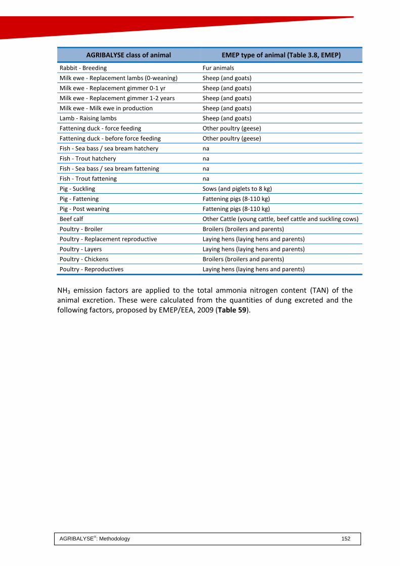
AGRIBALYSE®: Methodology 152
AGRIBALYSE class of animal EMEP type of animal (Table 3.8, EMEP)
Rabbit - Breeding Fur animals
Milk ewe - Replacement lambs (0-weaning) Sheep (and goats)
Milk ewe - Replacement gimmer 0-1 yr Sheep (and goats)
Milk ewe - Replacement gimmer 1-2 years Sheep (and goats)
Milk ewe - Milk ewe in production Sheep (and goats)
Lamb - Raising lambs Sheep (and goats)
Fattening duck - force feeding Other poultry (geese)
Fattening duck - before force feeding Other poultry (geese)
Fish - Sea bass / sea bream hatchery na
Fish - Trout hatchery na
Fish - Sea bass / sea bream fattening na
Fish - Trout fattening na
Pig - Suckling Sows (and piglets to 8 kg)
Pig - Fattening Fattening pigs (8-110 kg)
Pig - Post weaning Fattening pigs (8-110 kg)
Beef calf Other Cattle (young cattle, beef cattle and suckling cows)
Poultry - Broiler Broilers (broilers and parents)
Poultry - Replacement reproductive Laying hens (laying hens and parents)
Poultry - Layers Laying hens (laying hens and parents)
Poultry - Chickens Broilers (broilers and parents)
Poultry - Reproductives Laying hens (laying hens and parents)
NH3 emission factors are applied to the total ammonia nitrogen content (TAN) of the animal excretion. These were calculated from the quantities of dung excreted and the following factors, proposed by EMEP/EEA, 2009 (Table 59).

AGRIBALYSE®: Methodology 153
Table 59: Percentage of TAN in excreta for each type of animal (EMEP/EEA, 2009)
EMEP type of animal
% TAN/total N mass
Broilers (broilers and parents) 70%
Dairy cows 50%
Fattening pigs (8-110 kg) 70%
Fur animals 60%
Laying hens (laying hens and parents), 70%
Other cattle (young cattle, beef cattle and suckling cows) 0.6
Other poultry (ducks) 70%
Other poultry (geese) 70%
Other poultry (turkeys) 70%
Sheep (and goats) 50%
Sows (and piglets to 8 kg) 70%
The NH3 emissions were then calculated for liquid and solid manure in buildings (EF_building), in outdoor runs (EF_yard)6 and during storage (EF_storage). For missing values, average factors or default factors were used. Poultry dung was considered as solid manure. Table 60 gives the emissions factors used.
Table 60: NH3 emission factors for buildings (EF_building), outdoor runs (EF_yard) and storage (EF_storage) used for AGRIBALYSE
EMEP type of animal Type of excretion Source of emissions EF NH3
Broilers (broilers and parents) EF_pât 0,10
liquid EF_fertorg 0,55
solid EF_fertorg 0,79
Dairy cows EF_pât 0,10
liquid EF_fertorg 0,55
solid EF_fertorg 0,79
Fattening pigs (8-110 kg) liquid EF_fertorg 0,40
solid EF_fertorg 0,81
Fur animals EF_pât
liquid EF_fertorg
solid EF_fertorg
Laying hens (laying hens and parents), liquid EF_fertorg 0,69
solid EF_fertorg 0,69
6 As only the quantities in buildings and the quantities stored are entered in the data collection module, the
outdoor run emission factors are not used. However, they were included in the data collection module so that the model could be improved in a subsequent version.

AGRIBALYSE®: Methodology 154
EMEP type of animal Type of excretion Source of emissions EF NH3
Other Cattle (young cattle, beef cattle and suckling cows)
EF_pât 0,06
liquide EF_fertorg 0,55
solide EF_fertorg 0,79
Other poultry (ducks) EF_pât
liquide EF_fertorg
solide EF_fertorg 0,54
Other poultry (geese) EF_pât
liquide EF_fertorg
solide EF_fertorg 0,45
Other poultry (turkeys) EF_pât
liquide EF_fertorg
solide EF_fertorg 0,54
Sheep (and goats) EF_pât 0,09
liquide EF_fertorg
solide EF_fertorg 0,90
Sows (and piglets to 8 kg) EF_pât
liquide EF_fertorg 0,29
solide EF_fertorg 0,81
Others liquide EF_fertorg 0,4
solide EF_fertorg 0,81
Facteur moyen EF_pât 0,09
liquide EF_fertorg 0,51
solide EF_fertorg 0,71
3 Parameters for livestock and plant production: Organic fertilizer, grazing
The EMEP/EEA approach implies using different emission factors (EF) for calculating emissions during grazing or while spreading organic fertilizer. Different factors are used for grazing (EF_graze) and for spreading organic fertilizer (EF_orgfert). These factors apply to the quantity of Total Ammoniacal Nitrogen (TAN) and depend on the type of organic fertilizer used, whether it is liquid or solid, the source of emissions (grazing or not) and the form of application (see Table 61). No specific factor was available for organic fertilizers not derived from animal excreta and so an average emission factor was used. The percentage of TAN is given in Appendix H (column N-NH4
+) for organic fertilizers derived from animal excreta and in Table 62 for other organic fertlizers.

AGRIBALYSE®: Methodology 155
Table 61: Emission factors used in AGRIBALYSE for organic fertilizers
EMEP type of animal Form of fertilizer Source of emissions EF NH3
Broilers (broilers and parents) EF_graze 0.10
liquid EF_orgfert 0.55
solid EF_orgfert 0.79
Dairy cows EF_graze 0.10
liquid EF_orgfert 0.55
solid EF_orgfert 0.79
Fattening pigs (8-110 kg) liquid EF_orgfert 0.40
solid EF_orgfert 0.81
Fur animals EF_graze
liquid EF_orgfert
solid EF_orgfert
Laying hens (laying hens and parents), liquid EF_orgfert 0.69
solid EF_orgfert 0.69
Other Cattle (young cattle, beef cattle and suckling cows)
EF_graze 0.06
liquid EF_orgfert 0.55
solid EF_orgfert 0.79
Other poultry (ducks) EF_graze
liquid EF_orgfert
solid EF_orgfert 0.54
Other poultry (geese) EF_graze
liquid EF_orgfert
solid EF_orgfert 0.45
Other poultry (turkeys) EF_graze
liquid EF_orgfert
solid EF_orgfert 0.54
Sheep (and goats) EF_graze 0.09
liquid EF_orgfert
solid EF_orgfert 0.90
Sows (and piglets to 8 kg) EF_graze
liquid EF_orgfert 0.29
solid EF_orgfert 0.81
Sundry liquid EF_orgfert 0.81
solid EF_orgfert 0.40
Average factor EF_graze 0.09
liquid EF_orgfert 0.51

AGRIBALYSE®: Methodology 156
EMEP type of animal Form of fertilizer Source of emissions EF NH3
solid EF_orgfert 0.71
These emission factors can be adjusted using a correction factor depending on the
application method. However, lack of data on the application methods for any of the
fertilizers identified made it impossible to use correction factors.
Table 62: TAN content for organic fertilizers from outside the farm
Organic fertilizer not from the farm kg TAN/t or m3
Limed sewage sludge 5.32
Liquid sewage sludge 2.13
Semi-solid sewage sludge 3.20
Dried sewage sludge 1.,80
Manure / slurry compost 0.83
Household waste compost 0.62
Green waste compost 0.83
Sugar scum (alkaline amendment) 0.96
Feather meal 6.50
Vegethumus 0.92
Concentrated sugar beet vinasse 0.96
Distillery vinasse 0.96
Unspecified organic fertilizer (Mixtures of organic fertilizers) (t N) 50.00
4 Parameters for plant production: mineral fertilizers
The EMEP/CORINAIR (2006) methodology was used. The recommendations of the group of experts led by CITEPA were followed rather than those of EMEP/EEA (2009) for producing the national inventories to avoid methodological bias (Joya et al, 2012). Using the EMEP/EEA (2009) methodology, the emission factors are calculated depending on the form of mineral nitrogen fertilizer, the average spring temperature (spring starts when the sum of temperatures since January 1st reaches 400°C and lasts for 3 months) and possibly on an alkaline soil. The working group found a problem with respect to the definition of the average spring temperature: “… it can be seen that spring starts fairly late in cold regions but as these regions tend to be continental regions with markedly different seasons, the temperature in spring is higher than in warmer regions. The experts present agreed that taking account of temperature as suggested in the EMEP/EEA (2009) model was not representative of temperatures for spreading mineral fertilizers and that there seemed to be significant bias in the method proposed. Therefore, CITEPA decided to continue to use the methodology based on EMEP 2006 until a new methodology was available at national level.” The emission factors used by AGRIBALYSE are listed in Table 63. They apply to the total amount of nitrogen applied. For all applications of nitrogen when the form is not specified

AGRIBALYSE®: Methodology 157
(described as “N unspecified) a weighting factor was used (depending on the composition of the “French average fertilizer”, see Appendix I).
Table 63: Emission factors selected for mineral fertilizers
Type of fertilizer – EMEP name Emission factor (%)
kg NH3-N/kg total N applied)
Anhydrous ammonia 4
Ammonium nitrate 2
Calcium ammonium nitrate 2
Di-ammonium phosphate 5
N fertilizer French average (weighting factor) 5.9
Di-ammonium fertilizer 5
Mono-ammonium phosphate, other NP, NK and NPK fertilizer
2
Urea ammonium nitrate solution 8
Ammonium sulfate 8
Urea 15
5 Parameters for Thai rice
Assumptions: Rice-growing period = 120 days In the production systems studied the rice was not transplanted. However, urea was applied one month after sowing, which corresponds to the transplantation period. This was the emission factor considered.
According to FAO statistics (2002) and in agreement with observations during the period 2010-2011 in the zones studied, urea and ammonia based fertilizers account for 85% of the total nitrogen fertilizers applied to paddy fields in northern and north-eastern Thailand.
The bibliographic study carried out by Yan et al (2003b) focused on NH3 emissions from urea fertilization, the most commonly used form in south east Asia. The period and application method have a significant effect on the volatilization rate. Yan et al (2003b) proposed considering volatilization of 20% of the nitrogen applied when the fertilizer was incorporated while the plot was being prepared, 36% when the urea was applied after transplantation and 12% when the fertilizer was applied on formation of the panicle. Equation 5 was used to model the emissions. An average emission factor of 22% of the nitrogen applied can be calculated on the basis of the application of 30% of fertilizer while the plot was being prepared, 30% after planting and 40% on the formation of the panicle.
N-NH3 kg.ha-1 urea = (Uinc x 0.2) + (Utrans x 0.36) + (Upan x 0.12) x 0.46 (Equation 1)
Where:
0.46 is the conversion factor for N-urea

AGRIBALYSE®: Methodology 158
Uinc is the amount of urea applied and incorporated into the soil while the plot is being prepared
Utrans is the amount of urea applied during transplantation, during the growing phase
Upan is the amount of urea applied on formation of the panicle
The lack of experimental data made it impossible to define specific emission factors for the other forms of fertilizer. Based on EEA recommendations, Yan et al (2003b) suggested using the NH3 emission factors given in Table 64. They also recommended considering a basic emissions of 1.5 kg N-NH3.ha-1.year-1.
Table 64: Emission factors for mineral fertilizers applied to paddy fields
Type of fertilizer Emission factor (%)
kg NH3-N/kg total N applied)
Ammonia bicarbonate 33
Ammonium sulfate 22
Ammonium phosphate 5
Other forms 2
Compound fertilizer (NPK) 2
The total NH3 emissions can be calculated using Equation 2.
N-NH3 kg.ha-1 = [N-NH3 urea] + (N-AB x 0.33) + (N-AS x 0.22) + (N-AP x 0.05) + (N-Other x 0.02) + (1.5 kg N-NH3.ha-1.year-1 * D/365) (Equation 2)
Where:
N-NH3 urea is the N emissions from urea (see Equation 1)
N-AB is the quantity of N in the form of ammonium bicarbonate (kg.ha-1)
N-AS is the quantity of N in the form of ammonium sulfate (kg.ha-1)
N-AP is the quantity of N in the form of ammonium phosphate (kg.ha-1)
N-Other is the quantity of N in another form of nitrogen (kg.ha-1)
D is the effective duration of the crop period
(1.5 kg N-NH3.ha-1.year-1 * D/365): base emissions, adjusted for the period D
17/14 is the conversion factor between N- NH3 and NH3

AGRIBALYSE®: Methodology 159
Datasheet 2: Excretion of nitrogen by livestock
1 General information
Table 65: Models selected for each source of emissions
Source of emissions Model selected
Dairy cows CORPEN 1999(a)
Suckler beef, growing or fattening (suckler and dairy)
CORPEN 2001
Pigs CORPEN 2003
Poultry CORPEN 2006
Rabbits CORPEN 1999(b)
Main principle of the models CORPEN (1999a, 1999b, 2001, 2003, 2006) proposes a methodology for calculating the total nitrogen excreted by the animals using mass balance. The total nitrogen ingested by the animal is calculated and then the nitrogen fixed by the animals is determined. The total quantity of nitrogen excreted is the difference. Equation 1 of the nitrogen excretion calculation is:
Nexcreted = Ningested - Nfixed (Equation 1) The quantities of nitrogen ingested per day per animal are calculated from the description of the feed mixes and rations distributed to the animals and the tables given by INRA (1988, 1989, 2007) and Sauvant et al (2004). Bibliography CORPEN, 2006. Estimation des rejets d’azote, phosphore, potassium, calcium, cuivre, zinc
par les élevages avicoles – Influence de la conduite alimentaire et du mode de logement des animaux sur la nature et la gestion des déjections. Ed CORPEN, Paris, France. 55 p.
CORPEN, 2003. Estimation des rejets d’azote, phosphore, potassium, cuivre et zinc des porcs – Influence de la conduite alimentaire et du mode de logement des animaux sur la nature et la gestion des déjections. Ed CORPEN, Paris, France. 41 p.
CORPEN, 2001. Estimation des flux d’azote, de phosphore et de potassium associés aux bovins allaitants et aux bovins en croissance ou à l’engrais, issus des troupeaux allaitants et laitiers, et à leur système fourrager. Ed CORPEN, Paris, France. 34 p.
CORPEN, 1999a. Estimation des flux d’azote, de phosphore et de potassium associés aux vaches laitières et à leur système fourrager – Influence de l’alimentation et du niveau de production. Ed CORPEN, Paris, France. 18 p.
CORPEN, 1999b. Estimation des rejets d’azote et de phosphore par les élevages cunicoles. 17 p.
INRA, 2007. Alimentation des bovins, ovins et caprins. Besoins des animaux – Valeurs des aliments. Ed Quae, Versailles, France. p307.
INRA, 1989. L’alimentation des animaux monogastriques : porc, lapin, volaille– 2ème édition. Ed INRA, Paris, France. p282.
INRA, 1988. L’alimentation des bovins, ovins et caprins. Ed INRA, Paris, France. p471.

AGRIBALYSE®: Methodology 160
Sauvant D., Perez J.-M. and Tran G., 2004. Tables de composition et de valeur nutritive des matières premières destinées aux animaux d’élevage – 2ème édition. Ed INRA, Paris, France. 301 p.
2 Parameters for livestock production: cattle
The quantities of nitrogen fixed by the classes of cattle in the AGRIBALYSE database are given in Table 66. Table 66: Nitrogen fixed by the various classes of cattle in the AGRIBALYSE database (CORPEN, 1999a)
Class of animal N (g) fixed per kg of weight gain or kg of milk produced
for dairy cows Dairy cow - Replacement heifers +2 years 24
Dairy cow - Replacement heifers 1-2 years 24
Dairy cow - Replacement heifers weaning-1 year 24
Dairy cow - Cull cows at end of life 16
Dairy cow - Calf ("1 week" - weaning) 29
Dairy cow - Calf (birth -"1 week") 29
Suckler cow - Replacement heifers +2 years 29
Suckler cow - Replacement heifers 0-1 year 29
Suckler cow - Replacement heifers 1-2 years 29
Suckler cow - Genitor bulls 29
Suckler cow - Suckler cows 29
Suckler cow - Cull cows at end of life 16
Suckler cow - Heifer 0-1 year 18
Fattening - Steer or heifer + 2 years 18
Fattening - Steer or heifer 1-2 years 18
Fattening - Calf <1 year 29
Veal 29
Dairy cows - Dairy cows in production 5.1
In accordance with the recommendations in CORPEN (1999a), the quantities of nitrogen fixed by dairy cows in production (meat, bone, hair, etc) were neglected.
3 Parameters for livestock production: pigs
The nitrogen retained in the body by pigs was calculated using equation 1:
𝑁 = 𝑒(−0.9385−0,0145∗𝐿𝑀𝐶)(0.915𝐿𝑊1,1009)
(0,7364+0,0044∗𝐿𝑀𝐶)
6.25 (Equation 1)
Where: N is the quantity of nitrogen fixed (kg) LW is the live weight of the animal (kg) LMC is the Lean Meat Content at the normal slaughter weight (%) The following LMCs were considered (Table 67).

AGRIBALYSE®: Methodology 161
Table 67: LMC of the various classes of pig in the AGRIBALYSE database (Source: personal communication by Sandrine Espagnol-IFIP, 12/07/2012)
Class of animal LMC (%) Sows and piglets 0.615
Sows 0.565
Pigs - Post weaning 0.615
Pigs - Fattening 0.615
4 Parameters for livestock production: poultry
The quantities of nitrogen fixed by the classes of poultry in the AGRIBALYSE database are given in Table 68. Table 68: Nitrogen fixed by the various classes of poultry in the AGRIBALYSE database (CORPEN, 2006)
Type of animal N (g) fixed per kg of live weight gain wrt. kg
egg Chicken 29.6
Turkey 35.2
Duck 29,6
Chicken organic 32.8
Chicken, Label 32.8
Turkey, Label 35.2
Fattened duck 33.2
Egg 17.4
5 Parameters for livestock production: rabbits
The quantities of nitrogen fixed by the classes of rabbit in the AGRIBALYSE database are given in Table 69. Table 69: Nitrogen fixed by the various classes of rabbit in the AGRIBALYSE database (CORPEN, 1999b)
Type of animal N (g) fixed per kg of live weight gain/kg of live weight Doe 36.25
Kit 32.48
Fattened animals 29.05

AGRIBALYSE®: Methodology 162
6 Parameters for livestock production: sheep and goats
The quantities of nitrogen fixed by the animals in the AGRIBALYSE database are given in Table 70. Table 70: Nitrogen fixed by the various classes of sheep and goats in the AGRIBALYSE database
Type of animal N fixed Units Milk goat - Kids (0 - 1 week) 26 g/kg live meat
Milk goat - Replacement goats 0-1 year 26 g/kg live meat
Milk goat - Replacement goats 1-2 years 26 g/kg live meat
Milk ewe - Replacement lambs (0-weaning) 26 g/kg live meat
Milk ewe - Replacement gimmer 0-1 an 26 g/kg live meat
Milk ewe - Replacement gimmer 1-2 years 26 g/kg live meat
Lamb - Lambs 0-weaning 26 g/kg live meat
Lamb - Lambs weaning-sale 26 g/kg live meat
Lamb - Replacement gimmers 1 year-2 years 26 g/kg live meat
Lamb - Replacement gimmers weaning-1 year 26 g/kg live meat
Lamb - Ewe in production 26 g/kg live meat
Lamb - Suckling lamb 26 g/kg live meat
Milk goat - Goats in production 5 g/l milk
Milk ewe - Ewe in production 8.5 g/l milk
The nitrogen fixed by sheep and goats in production (bone, meat, hair, etc) was neglected. Only the nitrogen exported in the milk was taken into account.

AGRIBALYSE®: Methodology 163
Datasheet 3: Carbon dioxide (CO2)
1 General information
Table 71: Models selected for each source of emissions
Source of emissions Model selected
Absorption by the plants ecoinvent v2 (Nemecek and Kägi, 2007)
Application of lime and urea IPCC 2006b Tier 1
Bibliography ANSES, 2008. Table Ciqual - Composition nutritionnelle des aliments. http
://www.afssa.fr/TableCIQUAL INRA, 2007. Alimentation des bovins, ovins et caprins. Besoins des animaux – Valeurs des
aliments. Ed Quae, Versailles, France. p307. INRA, 1989. L’alimentation des animaux monogastriques : porc, lapin, volaille– 2ème
édition. Ed INRA, Paris, France. p282. INRA, 1988. L’alimentation des bovins, ovins et caprins. Ed INRA, Paris, France. p471. IPCC, 2006b. Guidelines for national greenhouse gas inventories. Vol No 4: Agriculture,
forestry and other land use (AFOLU). Ed Eggleston S., Buendia L., Miwa K., Ngara T. and Tanabe K., Kanagawa, Japan.
Nemecek T. and Kägi T., 2007. Life Cycle Inventories of Swiss and European Agricultural Production Systems - Data v2.0 (2007). Ecoinvent report No. 15a. Ed Swiss Center for Life Cycle Inventories, Zurich and Dübendorf, Switzerland. p360.
Sauvant D., Perez J.-M. and Tran G., 2004. Tables de composition et de valeur nutritive des matières premières destinées aux animaux d’élevage – 2ème édition. Ed INRA, Paris, France. 301 p.
2 Parameters for plant production: carbon sequestered by the plants
The quantities of carbon sequestered by crops are calculated using the method proposed by Nemecek et Kägi (2007) based on the quantity of dry matter produced by the crops and the carbohydrate, fat, protein and fiber content. These are based on the tables published by INRA (1988, 1989, 2007), Sauvant et al (2004) and nutritional information tables published by ANSES (2008). The biomass components are multiplied by carbon content factors (Table 72).This carbon is considered neutral so far as climate change is concerned.
Table 72: Carbon content of the various groups of compounds (Vertregt and Penning de Vries, 1987)
Group C content (g/kg of DM)
Carbohydrate 0.444
Protein 0.535
Lipid 0.774

AGRIBALYSE®: Methodology 164
3 Parameters for plant production: emissions from liming
The quantities of carbonates applied during liming (”calcareous powder rock”, CaCO3, or dolomite, CaMg(CO3)2) are multiplied by their own emission factors (see IPCC 2006b, volume 4 chapter 11.3). Fertilizer containing added carbonate (eg: limestone ammonium nitrate, but not “nitrate of lime”, calcium nitrate, CaNO3) was taken into account using a factor to convert it into kg CaCO3 (see comment in IPCC 2006b on calculating M, p. 11.27). Equations used:
(1) 𝐶𝑂2 − 𝐶 𝐸𝑚𝑖𝑠𝑠𝑖𝑜𝑛𝑠 = (𝑀𝐿𝑖𝑚𝑒𝑠𝑡𝑜𝑛𝑒 ∗ 𝐸𝐹𝐿𝑖𝑚𝑒𝑠𝑡𝑜𝑛𝑒) + (𝑀𝐷𝑜𝑙𝑜𝑚𝑖𝑡𝑒 ∗ 𝐸𝐹𝐷𝑜𝑙𝑜𝑚𝑖𝑡𝑒) Where: CO2-C Emissions is the annual C emissions due to liming (tC/yr) M is the annual quantity of calcium carbonate (CaCO3) or dolomite (CaMg(CO3)2), (t/yr) EF is the emission factor, (tC): EFLimestone = 0.12 / EFDolomite = 0.13
(2) 𝐶𝑂2 𝐸𝑚𝑖𝑡𝑡𝑒𝑑 = (1) ∗ (44
12)
Where: CO2 Emitted is the quantity of CO2 emitted per year Liming is considered only for carrots, cider apples and alfalfa and was not considered for other plant products as there was insufficient time and data was not easily available. A sensitivity analysis was carried out in October 2013 to evaluate the impact of liming on sugar beet.
4 Parameters for plant production: emissions from the application of urea
According to IPCC 2006b, the emissions from the application of urea or urea ammonium nitrate are calculated by multiplying the quantity of urea (CO(NH2)2) by a specific emission factor. Equations used
(1) 𝐶𝑂2 − 𝐶 𝐸𝑚𝑖𝑠𝑠𝑖𝑜𝑛𝑠 = (𝑀 ∗ 𝐸𝐹) Where:
CO2-C Emissions is the annual C emissions from the application of fertilizer in the form of urea (tC/yr)
M is the annual quantity of fertilizer in the form of urea, (t/yr) EF is the emission factor, (tC): EFUrea = 0.20
(2) 𝐶𝑂2 𝐸𝑚𝑖𝑡𝑡𝑒𝑑 = (1) ∗ (44
12)
Where: CO2 Emitted is the quantity of CO2 emitted per year As there was no information on the type of fertilizer applied (use of “French average fertilizer) the CO2 emissions were calculated on the basis of the urea content in the fertilizer (see Appendix I).

AGRIBALYSE®: Methodology 165
Datasheet 4: Trace metals Seven trace metals are considered in the ETM model: cadmium, copper, zinc, lead, nickel, chromium and mercury.
1 General information
Table 73: Models selected for each source of emissions
Source of emissions Model selected
Leaching: French crops SALCA‐SM partially modified for
France (Freiermuth, 2006 et SOGREAH, 2007)
Runoff (by soil loss): French crops
Accumulation in or losses from the soil: French crops
Special French crops
Tropical crops Not taken into account
Bibliography Arvalis, 1998. Synthèse des résultats de l’enquête sur les ETM du blé tendre, du blé dur,
du pois protéagineux et de la pomme de terre récoltés en 1997 et 1998. Baize D., Deslais W. and Saby N., 2007. Teneurs an huit éléments traces (Cd, Cr, Cu, Hg,
Ni, Pb, Se, Zn) dans les sols agricoles en France - Résultats d'une collecte de données à l'échelon national. Simplified final report. Ed ADEME, Angers France. p 49.
Harmanescu M., Alda L.M., Bordean D.M., Gogoasa I. and Gergen I, 2011. Heavy metals health risk assessment for population via consumption of vegetables grown in old minig area; a case study: Banat County, Romania. Chemistry Central Journal 2011, 5:64.
TERRES INOVIA, 2013. Personal communication Freiermuth R., 2006. Modell zur Berechnung der Schwermetallflüsse in der
Landwirtschaftlichen Okobilanz. Agroscope FAL Reckenholz, Zürich, Suisse. http://www.agroscope.admin.ch/oekobilanzen/01194/
Houba V.J.G. and Uittenbogaard J., 1994. Chemical composition of various plant species. International Plant Analytical Exchange (IPE). Department of Soil Science und Plant Nutrition, Wageningen Agricultural University The Netherlands.Menzi H. and Kessler J., 1998. Heavy metal content of manures in Switzerland. In Martinez J. an d Maudet M.N. (eds): Proc. 8th International Conference on the FAO ESCORENA. Network on Recycling of Agricultural, Municipal and Industrial Residues in Agriculture (RAMIRAN 98), Rennes (F) May 26-29 1998, vol. 1, 495-506.
Perkow W. and Ploss H., 1994. Wirksubstanzen der Pflanzenschutz - und Schädlingsbekämpfungsmittel. Ed Blackwell Wissenschafts Verlag, Berlin, Germany. p314.
RMQS, 2013. Base de Données d’Analyses de Terres. http://www.gissol.fr/programme/rmqs/rmqs.php
Schultheiss U., Roth U., Döhler H. and Eckel H, 2004. Erfassung von Schwermetallströmen in landwirtschaftlichen Tierproduktionsbetrieben und Erarbeitung einer Konzeption zur Verringerung der Schwermetalleinträge durch Wirtschaftsdünger tierischer Herkunft in Agrarökosysteme, 2004. Umweltbundesamt: Berlin. p130.

AGRIBALYSE®: Methodology 166
SOGREAH, 2007. Bilan des flux de contaminants entrants sur les sols agricoles de France métropolitaine. Ed ADEME, Angers, France. p330.
Thöni L. and Seitler E., 2004. Deposition von Luftschadstoffen in der Schweiz. Moosanaly- sen 1990-2000. Umwelt-Materialien Nr. 180. Bern: Bundesamt für Umwelt, Wald und Landschaft BUWAL.
Wolfensberger and Dinkel, 1997. Beurteilung nachwachsender Rohstoffe in der Schweiz in den Jahren 1993 – 1996. Im Auftrag des Bundesamtes für Landwirtschaft. Eidgenössische Forschungsanstalt für Agrarwirtschaft und Landtechnik, Tänikon.
2 Parameters for plant production
The SALCA-ETM model is based on mass balance by subtracting the mass of the trace metals in the outputs (the harvested product, co-products exported from the plot, leaching and soil loss into surface water, cf. figure 15) from the mass of the trace metals in the inputs (trace metals contained in the seeds, fertilizers and pesticides as well as the deposition of airborne trace metals). The difference in these flows is considered as emissions to the soil. These emissions may be negative, when the output masses are greater than the input masses. Considering uncertainties resulting from the parameters used, a negative balance should not be considered to indicate that the crops absorb metals and remove them from the soil. Only the outputs which actually leave the field are included in this mass balance: the trace metals in the crop residues left on the field (eg: straw from cereals that is not exported, prunings, wood from fruit trees) were not taken into account and were considered as remaining in the soil.
Figure 15: Schematic of the trace metal model used for AGRIBALYSE
INP1 – INP4 = inputs due to / influenced by agricultural practices INP5 = “background process”, independent of agricultural practices allocation factor = (Σ INP1-INP4)/(Σ INP1-INP5)
For all trace metals (Cd, Cu, Dr, Hg, Pb, Zn)
Inputs
Total inputs
(INP1) Seed (INP2) Fertilizer (min/org (INP3) Fungicides
(INP4) Grazing
(INP5) Deposition from the air
agricultural
allocation factor
non agricultural
Output
Total outputs
(OUT1) Product or grazed grass
(OUT2) Leaching
(OUT3) Erosion /
surface water
Δ=(OUT4) = emissions
into the soil
Plot / soil
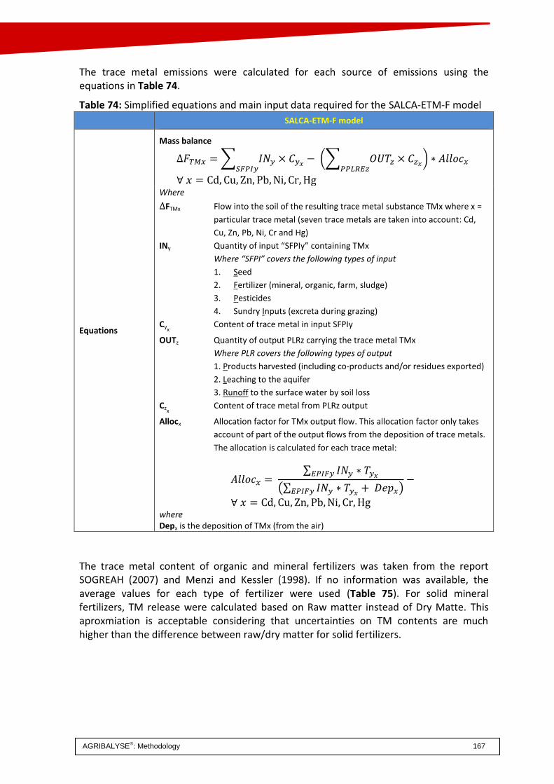
AGRIBALYSE®: Methodology 167
The trace metal emissions were calculated for each source of emissions using the equations in Table 74.
Table 74: Simplified equations and main input data required for the SALCA-ETM-F model
SALCA-ETM-F model
Equations
Mass balance
∆𝐹𝑇𝑀𝑥 = ∑ 𝐼𝑁𝑦𝑆𝐹𝑃𝐼𝑦
× 𝐶𝑦𝑥− (∑ 𝑂𝑈𝑇𝑧
𝑃𝑃𝐿𝑅𝐸𝑧× 𝐶𝑧𝑥
) ∗ 𝐴𝑙𝑙𝑜𝑐𝑥
∀ 𝑥 = Cd, Cu, Zn, Pb, Ni, Cr, Hg
Where
∆FTMx Flow into the soil of the resulting trace metal substance TMx where x =
particular trace metal (seven trace metals are taken into account: Cd,
Cu, Zn, Pb, Ni, Cr and Hg)
INy Quantity of input “SFPIy” containing TMx
Where “SFPI” covers the following types of input
1. Seed
2. Fertilizer (mineral, organic, farm, sludge)
3. Pesticides
4. Sundry Inputs (excreta during grazing)
Cyx Content of trace metal in input SFPIy
OUTz Quantity of output PLRz carrying the trace metal TMx
Where PLR covers the following types of output
1. Products harvested (including co-products and/or residues exported)
2. Leaching to the aquifer
3. Runoff to the surface water by soil loss
Czx Content of trace metal from PLRz output
Allocx Allocation factor for TMx output flow. This allocation factor only takes
account of part of the output flows from the deposition of trace metals.
The allocation is calculated for each trace metal:
𝐴𝑙𝑙𝑜𝑐𝑥 = ∑ 𝐼𝑁𝑦𝐸𝑃𝐼𝐹𝑦 ∗ 𝑇𝑦𝑥
(∑ 𝐼𝑁𝑦𝐸𝑃𝐼𝐹𝑦 ∗ 𝑇𝑦𝑥+ 𝐷𝑒𝑝𝑥)
−
∀ 𝑥 = Cd, Cu, Zn, Pb, Ni, Cr, Hg where Depx is the deposition of TMx (from the air)
The trace metal content of organic and mineral fertilizers was taken from the report SOGREAH (2007) and Menzi and Kessler (1998). If no information was available, the average values for each type of fertilizer were used (Table 75). For solid mineral fertilizers, TM release were calculated based on Raw matter instead of Dry Matte. This aproxmiation is acceptable considering that uncertainties on TM contents are much higher than the difference between raw/dry matter for solid fertilizers.

AGRIBALYSE®: Methodology 168
Table 75: Trace metal content of fertilizers (SL = sludge, CO = compost/unspecified organic matter, MF = mineral fertilizer, MA = manure, LI = slurry). The names for ecoinvent LCI data sets are used for the mineral fertilizers.
Type Fertilisant Teneur (en mg/kg MS)
MS Cd Cu Zn Pb Ni Cr Hg Source
SL Limed sewage sludge 40% 1,6 287,3 629,9 82,3 24,8 41,2 1,7 SOGREAH (2007)
SL Composted sewage sludge 29%
1,62 152,1 404,9 61,8 25,8 50,5 2,2 SOGREAH (2007), STEP
SL Liquid sewage sludge 6% 1,6 287,3 629,9 82,3 24,8 41,2 1,7 SOGREAH (2007)
SL Dried sewage sludge 93%
1,6 339 945 97 32 76,2 1,8 Menzi et Kessler (1998)
SL Sugar beet vinasse 26% 0,64 21,5 52,93 3,2 3 8,7 0,15 SOGREAH (2007)
SL Concentrated sugar beet vinasse 55% 0,64 21,5 52,93 3,2 3 8,7 0,15 SOGREAH (2007)
CO Manure / slurry compost 52%
1 249,5 626 45,17 34,74 53,52 0,2 SOGREAH (2007), déjections animales
CO Household waste compost 52%
4,62 164,37 554,28 325,92 60,35 126,34 1,64 SOGREAH (2007), OM
CO Green waste compost 52%
1,07 109,77 325,66 106,05 25,51 42,81 0,63 SOGREAH (2007), biodéchets
CO Feather meal 100%
0,2 7,3 135,3 8,3 2,8 65 0,1 Menzi et Kessler (1998)
MF Ammonium nitrate 100% 0,7 5,8 1,7 0,6 1 6,5 0,1 SOGREAH (2007)
MF Ammonium sulphate 100%
0,2 4,3 7,2 1 4,4 7,2 0 SOGREAH (2007), simple N
MF Average mineral fertilizer, as K2O 100%
0,01 2,32 0,44 0,05 0,15 0,1 0 SOGREAH (2007), simple K
MF Average mineral fertilizer, as N 100%
0,2 4,3 7,2 1 4,4 7,2 0 SOGREAH (2007), simple N
MF Average mineral fertilizer, as P2O5 100%
15,26 16,4 226 2,86 27,4 154 0,04 SOGREAH (2007), simple P
MF Calcium ammonium nitrate 100% 0,7 5,8 1,7 0,6 1 6,5 0,1 SOGREAH (2007),
MF Calcium nitrate 100%
0,2 4,3 7,2 1 4,4 7,2 0 SOGREAH (2007), simple N
MF Diammonium phosphate 100%
14,15 26,9 230,73 1,63 27,62 199,26 0 SOGREAH (2007), MAP DAP
MF Lime, from carbonation 100%
0,15 4 12,6 0,7 2,25 3,9 0,02 SOGREAH (2007), Carbonates
MF Limestone, milled, loose 100%
0,35 6,3 8,85 2,5 2,5 6,18 0,25 SOGREAH (2007), Chaux calquiqes
MF Magnesium oxide
100% 1,05 5,2 12,55 2,5 3,7 14,2 1,6
SOGREAH (2007), Chaux magnésiennes
MF Monoammonium phosphate 100%
14,15 26,9 230,73 1,63 27,62 199,26 0 SOGREAH (2007), MAP DAP
MF Nitric acid 100%
0 0 0 0 0 0 0 Menzi et Kessler (1998)
MF Potassium chloride
100% 0,23 3,53 5,19 0,81 2,67 1,28 0,05
SOGREAH (2007), clorure de potassium
MF Potassium nitrate 100%
6,17 16,89 124,83 2,51 14,37 84,35 0,22 SOGREAH (2007), NK / NPK
MF Potassium sulphate
100% 0,14 5,87 10,98 0,59 1,94 3,74 0,07
SOGREAH (2007), sulfat de potassium

AGRIBALYSE®: Methodology 169
Type Fertilisant Teneur (en mg/kg MS)
MS Cd Cu Zn Pb Ni Cr Hg Source
MF Single superphosphate
100% 12,3 18,38 190,77 2,35 25,13 97,38 0,11
SOGREAH (2007), autres superphosphat
MF Triple superphosphate 100%
19,56 30,97 406,56 3,57 32,2 196,94 0,12 SOGREAH (2007), TSP
MF Urea ammonium nitrate 100%
0,2 0,3 1,7 0,2 0,1 0 0,2 SOGREAH (2007), urée1)
MF Urea 100%
0,2 0,3 1,7 0,2 0,1 0 0,2 SOGREAH (2007), urée1)
MA Cattle manure 19%
0,3 23 119 3,8 4,4 7,5 0,13 SOGREAH (2007) Bovin - fumier
MA Compost bedded cattle manure 22%
0,3 23 119 3,8 4,4 7,5 0,13 SOGREAH (2007) Bovin - fumier
MA Cattle manure heap 31%
0,21 115,3 746,5 1,76 8,6 6,7 0,8 Menzi et Kessler (1998)
MA Pig manure 60%
0,2525
39,6 468,4 2,235 7,9 5,5 0,2 Menzi et Kessler (1998)
MA Layer hen manure 68%
0,292 43,8 349,2 2,92 40 10 0,2 Menzi et Kessler (1998)
MA Broiler manure 8%
0,178 37,1 162,2 3,77 4,3 3,9 0,4 Menzi et Kessler (1998)
LI Cattle slurry 5%
0,16 19,1 123,3 2,92 3,1 2,1 0,4 Menzi et Kessler (1998)
LI Thin cattle slurry 4%
0,21 115,3 746,5 1,76 8,6 6,7 0,8 Menzi et Kessler (1998)
If no information default average value for each type of fertilizer 42%
SL Limed sewage sludge 42% 1,28 184,79 452,6 54,97 18,9 37,77 1,28
SL Composted sewage sludge 58% 1,72 132,74 410,31 121,36 30,85 71,92 0,64
SL Liquid sewage sludge 100% 5,19 13,58 94,81 1,53 11,15 58,53 0,16
SL Dried sewage sludge 41% 0,28 44,62 320,18 3,05 11,62 7,45 0,27
SL Sugar beet vinasse 8% 0,19 71,7 444,63 2,55 6,15 4,85 0,6
1) corrected for Cu, Ni, Pb, Hg These data are based on technical instutes’ references in priority, else SALCA data were used, and if note was available average data for each ferilizer type was used.
Table 76 gives the copper and zinc content in phytosanitary products (SOGREAH 2007, Perkow and Ploss 1994).
Table 76: Copper and zinc content in active substances in phytosanitary products. For copper and zinc based phytosanitary products, emissions to the environment were calculated using the “phytosanitary model” instead of SALCA-ETM. The following substances were taken into account in both models as their composition was more complex (trace metal plus active substance).
Active substance Content (g/g)
Cu Zn Source
Mancozeb 0.025 SOGREAH (2007) p 53
Metiram zinc 0.18 SOGREAH (2007) p 53
Propineb 0.22 Perkow and Ploss (1994)
Zineb 0.24 Perkow and Ploss (1994)
Ziram 0.21 Perkow and Ploss (1994)

AGRIBALYSE®: Methodology 170
The trace metal contents for seeds, products and co-products harvested and exported from the field were based on Schultheiss et al (2004) or, if available, on more recent data from the Technical Institutes. The trace metal content of seeds was allocated to that of the products. If no information was available, the average values (allocated to product and co-product) were used (Table 77). If the values measured did not exceed the detection limit, the detection limit was taken as the value (if it was known).
Table 77: Trace metal content of products and co-products. The same values were used for seeds as for the products except for maize.
Product Content (mg/kg DM)
Cd Cu Zn Pb Ni Cr Hg % MS Source
Sugar beet 0.4 12 36.4 1.16 1.08 1.775 0.095 23 Houba and Uittenbogaard (1994)
Durum wheat 0.069 4.54 22 0.014 0.06 0.045 0.001 85 Arvalis (1998)
Durum wheat – straw
0.2 2.5 9.6 0.6 0.6 0.7 0 85 Schultheiss et al (2004)
Soft wheat 0.048 3.76 17.17 0.13 0.16 0.2 0.012 85 Arvalis (1998)
Soft wheat – straw 0.2 2.5 9.6 0.6 0.6 0.7 0 85 Schultheiss et al (2004)
Carrots 0.1 7.18 19.9 0.58 0.39 0 0 10,3 Hermanescu et al (2011)
1)
Rapeseed 0.047 4.74 39 0.035 0.57 0.22 0.007 91 TERRES INOVIA (2013)
Alfalfa 0.13 8.6 40 1.2 1.68 1.09 0.15 30 Houba and Uittenbogaard (1994)
Silage maize 0.1 5 34.5 1.61 0.48 0.7 0.01 81 Houba and Uittenbogaard (1994)
Grain maize 0.03 2.5 21.5 0.3 1.16 0.32 0 72 Houba and Uittenbogaard (1994)
Seed maize 0,03 2,5 21,5 0,3 1,16 0,32 0 85 Houba and Uittenbogaard (1994)
Barley 0.03 4.3 26.6 0.2 0.1 0.1 0 85 Schultheiss et al (2004)
Barley- straw 0.1 4.8 11.1 0.6 0.8 1.2 0 85 Schultheiss et al (2004)
Peas 0.018 6.65 24.71 0.15 1.73 0.82 0.002 85 Arvalis (1998)
Potatoes 0.029 0.82 2.87 0.029 0.076 0.01 0.008 20 Arvalis (1998)
Permanent meadow 0.13 8.6 40 1.2 1.68 1.09 0.15 16,6 Houba and Uittenbogaard (1994)
Temporary grassland 0.13 8.6 40 1.2 1.68 1.09 0.15 16,6 Houba and Uittenbogaard (1994)
Sunflowers 0.358 17.1 47.1 0.047 1.9 0.18 0.0056 91 TERRES INOVIA (2013)
Triticale 0.1 4.3 28.4 0.2 0.2 0.1 0 85 Schultheiss et al (2004)
Triticale – straw 0.1 2.5 13.1 0.7 0.4 0.8 0 85 Schultheiss et al (2004)
Grapes 0,11 6,48 29,05 0,58 0,91 0,58 0,06 18 Average data used
Product, average 0.11 6.48 29.05 0.58 0.91 0.58 0.06 48 Average
Co-product, average 0.14 4.92 20.56 0.82 0.96 0.93 0.15 60 Average
1) for trace metals Cd, Cu, Zn, Ni and Pb (values for Carrot Root (ref) in Hermanescu et al (2011)). The average values were used for Cr and Hg.
Values for deposition from the air were also taken from SOGREAH (2007).

AGRIBALYSE®: Methodology 171
Table 78: Deposition of trace metals from the air in mg per hectare in France and Switzerland
Country Content (mg/ha/year)
Cd Cu Zn Pb Ni Cr Hg Source
France 200 8000 55000 8000 3000 2000 90 SOGREAH (2007) p 296; France – rural area
Switzerland 700 2400 90400 18700 5475 3650 50 Thöni and Seitler (2004)
All trace metal emissions (leaching, runoff and soil emissions) are multiplied by an allocation factor so that only emissions related to farming practices are taken into account. This allocation factor is calculated by dividing the sum of the inputs from agricultural activities (seed, fertilizer, phytosanitary products) by the sum of all the inputs (including deposition of trace metals from the air). For crops grown in soil based production in greenhouses (tomatoes) the deposition of trace metals from the air was not taken into account as the greenhouses prevent them being deposited on the cultivated soil.
3 Calculating leached trace metals
The quantities of trace metals leached to the aquifers were estimated by multiplying the average leaching per hectare per year (Table 79) by the period for which the crop was grown (see datasheet 11, Table 129) and the area occupied. As there was no data specific to France, data for Switzerland, taken from the original SALCA-ETM model was used for France. As the trace metals are strongly linked to the geology of the soil, the data for Switzerland should be used with care for the French average (Baize et al, 2007).
Table 79: Average leaching per ha per year
Country Average leaching (g per hectare per year)
Cd Cu Zn Pb Ni Cr Hg Source
Switzerland 0.05 3.6 33 0.6 0 21.2 0.0113 Wolfensberger und Dinkel, 1997
4 Calculating trace metal runoff
The quantities of trace metals emitted by runoff and soil loss in the surface water were calculated using:
The quantity of soil lost, in kg per hectare per year. This quantity is calculated using the soil loss model depending on the crop grown (see datasheet 5). If the period for which the crop is grown is greater than one year (eg: orchard, grassland), the soil loss model gives two values for the soil lost (for year 1 and for following years).
The land occupation duration (Table 129), The average trace metal content per kg of soil. These contents depend on the
category of the crop grown: arable, permanent meadow, special intensive crop and grapevines. The data used was the total content and was taken from the BDAT

AGRIBALYSE®: Methodology 172
database (RMQS, 2013). As only one value was available for mercury for arable crops, this value was used for all soil uses (Table 80).
An eroded particle enrichment factor of 1.86 and a fraction of eroded earth arriving at a watercourse of 0.2 (Freiermuth R., 2006).
Table 80: Average content of trace metals in soils in France depending on the soil use
Type of crop Content (mg/kg of soil)
Cd Cu Zn Pb Ni Cr Hg Source
Permanent meadow 0.299 20.402 87.188 36.69 28.923 63.389 0.068 RMQS (2013)
Arable crops 0.318 20.939 69.745 29.461 24.121 55.162 0.068 RMQS (2013)
Intensive crops 0.299 53.443 82.448 36.702 27.98 47.295 0.068 RMQS (2013)
Grapevines 0.178 87.244 63.703 27.368 23.088 50.363 0.068 RMQS (2013)
5 Parameters for excretions during grazing
Trace metals from excretions during grazing were taken into account using an approach similar to the manure spreading. As the grazed grass data sets were based on grazing by cattle (see chapter B.2.7.7), the trace metal contents of cattle dung were used (Table 75).
6 Parameters for tropical crops
As there was no data for the trace metal contents in tropical soils or for deposition from the air, the trace metal flows were not calculated for tropical crops.
7 Parameters for livestock production
Any emissions during storage (at the side of fields, in ditches, etc.) were not taken into account assuming that the excretions were stored enclosed for most of the time.

AGRIBALYSE®: Methodology 173
Datasheet 5: Soil loss
1 General information
The RUSLE soil loss equation (Foster, 2005) was used with appropriate parameters. Bibliography AGRESTE, 2006. Enquête sur les pratiques culturales en 2006.
http://agreste.agriculture.gouv.fr/page-d-accueil/article/donnees-en-ligne.
Foster G. R., 2005. Revised Universal Soil Loss Equation – Version 2 (RUSLE2). USDA – Agricultural Research Service, Washington D.C., p286.
Néboit-Guillot R., 1991. L’homme et l’érosion : L’érosion des sols dans le monde. Ed Presses Universitaires Blaise Pascal, Clermond-Ferrand, France. p269.
2 Parameters for plant production
The soil loss model applies only to crops grown in the open air. For soilless crops, the soil
loss is by default 0. The soil losses were calculated using the equation in Table 81.
Table 81: RUSLE soil loss equation
USDA RUSLE soil loss equation
A = R * K * LS * C * P * f
Where
A is the computed spatial and temporal average soil loss per unit area (t/ha/year)
R is the rainfall-runoff erosivity factor
K is the soil erodibility factor
L is the slope length factor
S is the slope steepness factor
C is the cover-management factor
P is the support practice factor
f is the acre => hectare conversion factor = 2.47
For R, the values used were based on the map by Néboit-Guilhot, 1991. When the map
was analyzed, a regional approach was considered and six main regions were defined
(Table 82).

AGRIBALYSE®: Methodology 174
Table 82: Values for R and K for each region defined. K was calculated (see below)
Region Region of France R K
Central R11 - Ile-de-France, R24 - Centre, R26 - Burgundy, R74 - Limousin, R83 – Auvergne
40 0.30
North R21 - Champagne-Ardenne, R22 - Picardy, R23 - Upper-Normandy, R25 - Lower-Normandy, R31 - Nord - Pas-de-Calais
30 0.35
North-East R41 - Lorraine, R42 - Alsace, R43 - Franche-Comté, R82 - Rhône-Alpes
50 0.29
West R53 – Brittany 30 0.35
South R73 - Midi-Pyrenees, R91 - Languedoc-Roussillon, R93 - Provence-Alpes-Côte d'Azur, R94 – Corsica
100 0.30
South-West R52 - Pays de la Loire, R54 - Poitou-Charentes, R72 - Aquitaine 80 0.31
K was calculated using the average soil composition (sand (0.05-2 mm), silt (0.002-
0.05mm) and clay (<0.002mm)) for each region. The soil losses were calculated using
RUSLE2, based on the GisSol database for the soil composition and information from INRA
for the regional rainfall.
For each of the six “soil loss regions” defined, a regional climate profile (with
temperature and rainfall data for 2005-2009) and a regional soil profile were
defined for RUSLE2 (Table 86 to Table 88)
The average soil loss was calculated by RUSLE2 using R for the region, a fixed slope
of 2% and default values for the other parameters (eg. “contour farming” for the
support practice, see P below)
The soil loss calculated was compared with the results from the AGRIBALYSE
model. K was modified until both models gave the same results.
Table 86 to Table 88 show the averaging procedure for calculating the regional soil
composition: Table 83 gives the effective agricultural area (EAA) and the average clay, silt
and sand content for each canton available in GisSol. The weightings were calculated
(Table 71) by dividing the effective agricultural area in the canton by the effective
agricultural area in the region. The weighted contents were added to give a weighted
mean (Table 85).

AGRIBALYSE®: Methodology 175
Table 83: Extract from the GisSol database: effective agricultural area (ha) and average sand, silt and clay content per canton (g/kg)
Extract from the GISSOL database
Period Beginning of 2000 to end 2004 Units Values in g/kg of soil Number of cantons 2731
Version version 3.3.0.0 of 09/07/2012. Canton Number EAA (ha) Sand Silt Clay
AMBERIEU-EN-BUGEY 101 4174 210.23 439.25 306.09
BAGE-LE-CHATEL 102 6572 415.48 384.94 112.8
BELLEGARDE-SUR-VALSERINE 103 0 261.75 0 167.91
BELLEY 104 6777 391.53 416.73 170.66
BRENOD 106 5401 205.93 430.14 250.25
CEYZERIAT 107 0 167.91 0 208.22
CHALAMONT 108 7653 244.39 594.33 144.61
CHAMPAGNE-EN-VALROMEY 109 6905 253.43 479.22 211.7
CHATILLON-SUR-CHALARONNE 110 16857 236.22 506.69 161.11
COLIGNY 111 9043 319.33 476.17 211.41
COLLONGES 112 4259 359.98 344.69 219.36
And 2720 other cantons
Table 84: Calculation of weighting per canton
Canton Region Weighting Sand Silt Clay AMBERIEU-EN-BUGEY NE 0.001281815 0.2694759 0.563037183 0.392350715
BAGE-LE-CHATEL NE 0.002018229 0.8385337 0.776897026 0.227656218
BELLEGARDE-SUR-VALSERINE NE 0 0 0 0
BELLEY NE 0.002081183 0.8148457 0.867291547 0.355174755
BRENOD NE 0.001658621 0.3415597 0.713439039 0.415069790
CEYZERIAT NE 0 0 0 0
CHALAMONT NE 0.002350199 0.5743650 1.396793573 0.339862229
CHAMPAGNE-EN-VALROMEY NE 0.002120492 0.5373961 1.016181958 0.448908060
CHATILLON-SUR-CHALARONNE NE 0.005176702 1.2228405 2.622983037 0.834018428
And 2722 other cantons
Table 85: Average per region (g/kg)
Soil loss region Total area (ha) Sand (g/kg) Silt (g/kg) Clay (g/kg) Central 6,200,572 333 426 218
North 5,556,017 208 574 213
North-East 3,256,320 279 448 265
West 1,277,126 278 546 172
South 2,570,232 347 416 234
South West 4,896,927 365 423 205
The average monthly temperatures and average monthly rainfall from 2005 to 2009 were
calculated from the data from the INRA weather station network (Climatik) by INRA,
Rennes (Emmanuelle Garrigues). The average values were calculated using the data from
a station close to the main town in each administrative region. The weighting factors

AGRIBALYSE®: Methodology 176
were calculated by dividing the agricultural areas used in the administrative region by the
area of the “soil loss region” (Table 88).
Table 86: Weather stations used to calculate the average temperatures and rainfall, grouped into six “soil loss” regions
Soil loss region
Administrative region Area
(km2)
Weighting Data source Weather station
CENTRAL Auvergne 26013 20.7% CLIMATIK Clermont-Ferrand
CENTRAL Burgundy 31582 25.1% NASA
CENTRAL Center 39151 31.1% CLIMATIK Champhol
CENTRAL Ile-de-France 12011 9.6% CLIMATIK Versailles
CENTRAL Limousin 16942 13.5% NASA
NORTH Lower-Normandy 17589 20.1% NASA
NORTH Champagne-Ardenne 25606 29.3% CLIMATIK Courcy
NORTH Upper-Normandy 12317 14.1% CLIMATIK Mons-en-Chaussée
NORTH Nord-Pas-de-Calais 12414 14.2% NASA
NORTH Picardy 19399 22.2% NASA
NORTH-EAST Alsace 8280 9.9% CLIMATIK Entzheim
NORTH-EAST Franche-Comté 16202 19.4% CLIMATIK Meythet
NORTH-EAST Lorraine 23547 28.2% CLIMATIK Tomblaine (Nancy)
NORTH-EAST Rhône-Alpes 43698 52.4% CLIMATIK Romans-sur-Isère
WEST Brittany 27208 100.0% CLIMATIK St Jacques de la Lande
SOUTH Corsica 8680 7.7% CLIMATIK Lucciana
SOUTH Languedoc-Roussillon 27376 24.3% CLIMATIK Mauguio
SOUTH Midi-Pyrenees 45348 40.2% CLIMATIK Blagnac
SOUTH Provence-Alpes-Côte d'Azur 31400 27.8% CLIMATIK Fourques
SOUTH-WEST Aquitaine 41309 41.6% CLIMATIK Cestas
SOUTH-WEST Pays de la Loire 32082 32.3% CLIMATIK Beaucouze
SOUTH-WEST Poitou-Charentes 25810 26.0% CLIMATIK Lusignan
Table 87: Weighted mean monthly rainfall for each soil loss region from 2005 to 2009
Reg./month CENTRAL NORTH NORTH-EAST WEST SOUTH SOUTH-EAST January 54.3 43.5 48.6 76.2 54.8 67.4
February 47.7 49.2 54.0 66.2 31.4 54.9
March 66.5 57.6 68.4 72.8 37.6 77.0
April 61.4 38.9 79.9 53.0 61.2 57.1
May 76.5 84.7 92.4 77.9 74.3 71.3
June 64.7 56.5 66.7 44.5 32.2 56.7
July 64.5 75.6 63.1 58.7 15.7 43.5
August 67.2 67.7 96.7 47.9 24.5 48.8
September 51.2 40.3 90.0 45.0 74.1 52.1
October 57.1 50.5 99.6 68.4 76.7 66.7
November 59.8 52.2 85.7 104.9 62.0 90.6
December 60,.7 55.7 64.2 87.0 48.9 71.7
Total 732.2 673.0 909.8 803.1 594.0 7582
% area 20.61 23.39 26.10 13.71 10.82 5.38

AGRIBALYSE®: Methodology 177
Table 88: Weighted mean monthly temperatures for each soil loss region from 2005 to 2009
°C CENTRAL NORTH NORTH-EAST WEST SOUTH SOUTH-EAST January 3.3 3.9 3.5 6.5 6.5 5.5
February 3.7 4.0 4.1 6.1 7.2 5.8
March 6.2 6.2 7.8 7.9 10.0 8.2
April 10.6 10.5 12.7 10.4 13.5 11.2
May 14.8 14.3 17.5 13.6 17.6 15.0
June 18.0 17.1 21.4 16.5 21.5 18.5
July 20.0 19.2 23.4 17.9 23.6 19.8
August 18.4 17.9 21.3 17.0 22.5 18.6
September 15.8 15.9 17.9 15.6 19.4 16.3
October 12.2 12.3 13.7 13.2 15.8 13.4
November 6.9 7.6 7.9 9.4 10.5 8.6
December 2.8 3.4 3.2 5.7 6.1 4.6
% area 20.61 23.39 26.10 13.71 10.82 5.38
These temperatures and rainfall were used to calculate K for each region shown in the
right hand column of Table 82. Different weighting approaches were possible for the
plant LCI data sets:
a) “French average” factors: R and K were weighted on the basis of the area of
agricultural area per region
b) regional weighting: R and K were weighted depending on the average EAA for 2005 to
2009 per region per crop, based on data from the annual agricultural statistics
(AGRESTE, 2005-2009) depending on the representativeness of the particular regions
used for the data set.
c) values from a particular region: some crops were characterized for clearly defined
regions (eg: carrots in Aquitaine, grassland in Auvergne). In these cases the factors for
the region concerned were used without modification.
The slope length LS was set to 30 m . A fixed value of 2% was used for the slope which
gave an LS of 0.27 (Table 89).
Table 89: Matrix for determining LS, based on data originally calculated for Michigan (http://www.iwr.msu.edu/rusle/lstable.htm)
Slope length in feet (top row) and meters (second row))
3 6 9 12 25 50 75 100 150 200 250 300 400 600 800
Slope 1 2 3 4 8 15 23 30 46 61 76 91 122 183 244
0.2% 0.05 0.05 0.05 0.05 0.05 0.05 0.05 0.05 0.05 0.05 0.05 0.05 0.05 0.06 0.06
0.5% 0.07 0.07 0.07 0.07 0.08 0.08 0.08 0.09 0.09 0.09 0.09 0.09 0.1 0.1 0.1
1% 0.11 0.11 0.11 0.11 0.12 0.13 0.14 0.14 0.15 0.16 0.17 0.17 0.18 0.19 0.2
2% 0.17 0.17 0.17 0.17 0.19 0.22 0.25 0.27 0.29 0.31 0.33 0.35 0.37 0.41 0.44
3% 0.22 0.22 0.22 0.22 0.25 0.32 0.36 0.39 0.44 0.48 0.52 0.55 0.6 0.68 0.75
4% 0.26 0.26 0.26 0.26 0.31 0.4 0.47 0.52 0.6 0.67 0.72 0.77 0.86 0.99 1.1
5% 0.3 0.3 0.3 0.3 0.37 0.49 0.58 0.65 0.76 0.85 0.93 1.01 1.13 1.33 1.49
6% 0.34 0.34 0.34 0.34 0.43 0.58 0.69 0.78 0.93 1.05 1.16 1.25 1.42 1.69 1.91

AGRIBALYSE®: Methodology 178
Slope length in feet (top row) and meters (second row))
3 6 9 12 25 50 75 100 150 200 250 300 400 600 800
Slope 1 2 3 4 8 15 23 30 46 61 76 91 122 183 244
8% 0.42 0.42 0.42 0.42 0.53 0.74 0.91 1.04 1.26 1.45 1.62 1.77 2.03 2.47 2.83
10% 0.46 0.48 0.5 0.51 0.67 0.97 1.19 1.38 1.71 1.98 2.22 2.44 2.84 3.5 4.06
C was calculated as the product of C1 and C2, i.e. depending on:
The type of crop
The type of tillage that causes the most soil loss using the following factors (Table
90). If several productions systems have been included in an average data set and
the soil is tilled using different methods, C2 was weighted depending on the
percentage of area concerned entered in the data collection module.
For soil-based crops grown in a greenhouse, C1 was taken to be the same as that used for orchards / fruit trees.
Table 90: Defining C1 and C2, depending on the type of crop and tilling method, source
http://www.omafra.gov.on.ca/english/engineer/facts/00-001.htm
C1 Type of crop C1
Fruit trees 0.10
Cereals (spring and fall) 0.35
Arable crop, not listed 0.42
Soil-based crop in greenhouse 0.05
Seasonal horticultural crop (including vine) 0.50
Hay and grazed grass 0.02
Beans, rapeseed, silage maize 0.50
Grain maize 0.40
C2 Soil tillage method C2
Stubble plowing 0.60
Fall tillage 1.00
Spring tillage 0.90
No-till 0.25
Strip till 0.25
Ridge planting 0.35
P represents the way in which the farmer works the plot depending on the relief: in the
direction of the slope or at right angles to it. P was set to 0.5 which is the value for
contour farming. Contour farming works the land at right angles to the slope (Table 91)
and reduces the risk of soil loss by runoff.

AGRIBALYSE®: Methodology 179
Table 91: Defining P depending on the orientation of the crop, source:
http://www.iwr.msu.edu/rusle/lstable.htm
Support Practice (USLE) P
Contour farming 0.50
Cross Slope 0.75
Strip cropping, contour 0.25
Strip cropping, cross slope 0.37
Up and Down Slope 1.00
3 Special cases
a) Permanent crop systems
The same approach was used for permanent crop systems (alfalfa, temporary grassland,
orchards, grapevines, coffee and clementines). As the crops are planted (tillage/sowing)
the first year only, the quantity of soil lost had to be calculated differently for years 2 to x
with C2 set to 0.25 (equivalent to no till).
b) Calculating R for clementines
R was calculated for clementines using average regional data for rainfall (Table 92) as 60.
K was 0.32 depending on the silt-clay content of the soil. Values for France were used for
the slope, C1, C2 and P.
Table 92: Monthly rainfall in Morocco. Source: CIRAD (2013)
JAN FEB MAR APRIL MAY JUNE JULY AUG SEP OCT NOV DEC
36.5 33.1 39.5 18.5 2.6 0.4 0.1 2.1 3.5 16.7 36.6 67.1
c) Soil loss for tropical crops
As no data was available for the calculations, the quantity of soil lost could not be
calculated and was taken to be zero for coffee (Brazil) and for rice (Thailand).
d) Soilless crops
There was no soil loss for soilless crops and the quantity of soil lost was zero.

AGRIBALYSE®: Methodology 180
Datasheet 6: Combustion emissions
1 General information
The model proposed in ecoinvent v2 (Nemecek and Kägi, 2007) was used with modifications. Bibliography Nemecek T. and Kägi T., 2007. Life Cycle Inventories of Swiss and European Agricultural
Production Systems - Data v2.0 (2007). Ecoinvent report No. 15a. Ed Swiss Center for Life Cycle Inventories, Zurich and Dübendorf, Switzerland. p360.
2 Parameters for plant and livestock production
16 substances emitted from burning fuel by powered machines are taken into account in ecoinvent v2 (Nemecek and Kägi, 2007). Two different formulae are used:
Ecoinvent formulae for CO, HC and NO, taking account of the speed and power of
the machine, are used to calculate standard emissions per hour of operation (g/h)
for each process considered. The standard values are then multiplied by the
operation time for the process.
The emission factors per kg of fuel consumed were calculated for the other
gaseous emissions. These factors are fixed and are the same for all processes.
In AGRIBALYSE, all the emissions were calculated using fixed emission factors per kg of fuel, assuming the same average speed and power.

AGRIBALYSE®: Methodology 181
Table 93: Emissions of substances for diesel and gasoline (Nemecek and Kägi, 2007)
Substance DIESEL (g/kg)
GASOLINE (g/kg)
Ammonia 0.0200 0.0400
Benzene 0.0073 9.4800
Benzo(a)pyrene) 3.0E-08 4.0E-05
Cadmium 1.0E-08 1.0E-05
Carbon dioxide, fossil 3120 3000
Carbon monoxide, fossil 5.4300 633
Chromium 5.0E-05 5.0E-05
Copper 0.0017 0.0017
NMVOC, non-methane volatile organic compounds 2.6500 10.9
Methane 0.1290 2.92
Nickel 7.0E-05 7.0E-05
Mono-nitrogen oxides (NOx) 41.8000 20.000
Dinitrogen oxide (N2O) 0.1200 0.1300
Particulates, < 2.5 um 4.3200 3.0200
Sulfur dioxide 1.0100 0.0720
Zinc 0.0010 0.0010
Heat, waste 45.4 MJ 45.1 MJ
Heating emissions (in greenhouses and livestock buildings) were included by multiplying the quantity of fuel by the existing ecoinvent LCI data sets (Table 94). As the greenhouse heating systems are included in the AGRIBALYSE greenhouse LCI data set, the ecoinvent LCI data sets had to be modified by removing the boiler input. Table 94: Heating systems and assignment to existing modified LCI data sets
Fuel ecoinvent LCI data set Comments Livestock production
Fuel oil Light fuel oil, burned in boiler 100kW condensing, non-modulating/MJ/CH
Natural gas Natural gas, burned in boiler condensing modulating <100kW/MJ/RER
Propane/butane Natural gas, burned in boiler condensing modulating <100kW/MJ/RER
Plant production
Waste wood Logs, softwood, burned in furnace of greenhouse/MJ/CH
No boiler (included in greenhouse LCI data set)
Coal Hard coal, burned in furnace of greenhouse/MJ/RER
Light fuel oil Light fuel oil, burned in furnace 1MW of greenhouse/MJ/RER
Heavy fuel oil Heavy fuel oil, burned in furnace 1MW of greenhouse/MJ/RER
Natural gas Natural gas, burned in furnace >100kW of greenhouse/MJ/RER
Propane Natural gas, burned in furnace >100kW of greenhouse/MJ/RER
Diesel Diesel, burned in cogen 200kWe of greenhouse/MJ/CH
Comment on “waste wood” fuel. There was no available LCI data set for “burning waste wood” or “waste wood” in ecoinvent 2.0. As the waste wood had to be prepared (eg shredded), the “soft wood” LCI data set was selected as a first estimate even though the impact was probably greater than waste wood.

AGRIBALYSE®: Methodology 182
Datasheet 7: Methane (CH4)
1 General information
Table 95: Models selected for each source of emissions
Source of CH4 emissions Model selected
Enteric emissions Cattle Sheep Goats Pigs Poultry
IPCC 2006b Tier 2 IPCC 2006b Tier 2 IPCC 2006b Tier 1 IPCC 2006b Tier 1 IPCC 2006b Tier 1
Excretions in buildings and during storage IPCC 2006b Tier 2
Excretions in grasslands and outdoor runs IPCC 2006b Tier 2
Thai rice IPCC 2006b Tier 2
Bibliography CORPEN, 2006. Estimation des rejets d’azote, phosphore, potassium, calcium, cuivre, zinc
par les élevages avicoles – Influence de la conduite alimentaire et du mode de logement des animaux sur la nature et la gestion des déjections. Ed CORPEN, Paris, France. p55.
IE, ITAVI, ITCF, ITP, 2001. Fertiliser avec des engrais de ferme. Ed. Arvalis, Paris, France. p101.
INRA, 2007. Alimentation des bovins, ovins et caprins. Besoins des animaux – Valeurs des aliments. Ed. Quae, Versailles, France. p307.
INRA, 1989. L’alimentation des animaux monogastriques : porc, lapin, volaille– 2ème édition. Ed. INRA, Paris, France. p282.
INRA, 1988. L’alimentation des bovins, ovins et caprins. Ed. INRA, Paris, France. p471. IPCC, 2006b. Guidelines for national greenhouse gas inventories. Vol No 4: Agriculture,
forestry and other land use (AFOLU). Ed Eggleston S., Buendia L., Miwa K., Ngara T. et Tanabe K., Kanagawa, Japan.
ITAVI, 2003. Caractérisation des fumiers, lisiers et fientes de volailles. Etude OFIVAL 2001. p41.
Levasseur, P., 2005. Composition des effluents porcins et de leurs coproduits de traitement – Quantités produites. p68.
Pouech P., 2009. Etude de caractérisation des fumiers de cheval issus de centres équestres afin d’aider à la décision sur les possibilités de valorisation. Rapport final. Étude APESA pour la FIVAL. p60.
Sauvant D., Perez J.-M. and Tran G., 2004. Tables de composition et de valeur nutritive des matières premières destinées aux animaux d’élevage – 2ème édition. Ed. INRA, Paris, France. 301 p.
Yan X., Ohara T. and Akimoto H., 2005. Statistical modeling of global soil NOx emissions. Global Biogeochemical Cycles 19(3). p15.

AGRIBALYSE®: Methodology 183
Yan X., Ohara T. and Akimoto H., 2003a. Development of region-specific emission factors and estimation of methane emission from rice fields in the East, Southeast and South Asian countries. Global Change Biology, 9: 237-254.
Yan X., Akimoto H. and Ohara T., 2003b. Estimation of nitrous oxide, nitric oxide and ammonia emissions from croplands in East, Southeast and South Asia. Global Change Biology, 9: 1080-1096.
2 Parameters for livestock production: enteric emissions
1. Animal class definitions Table 96: Correspondence between the AGRIBALYSE animal classes and the categories defined by the IPCC. Level of precision used to calculate the enteric methane emissions
AGRIBALYSE classes IPCC-enteric CH4 emission classes
Method
Suckler cow - Replacement heifers +2 yrs Other cattle Tier 2
Suckler cow - Replacement heifers 0-1 yr Other cattle Tier 2
Suckler cow - Replacement heifers 1-2 yrs Other cattle Tier 2
Suckler cow - Genitors Other cattle Tier 2
Suckler cow - Suckler cows Other cattle Tier 2
Suckler cow - Cull cows at end of life Other cattle Tier 2
Suckler cow - Calf 0-1 yr Other cattle Tier 2
Beef cattle - Fattened steer or heifer + 2 yrs Beef cattle Tier 2
Beef cattle - Fattened steer or heifer 1-2 yrs Beef cattle Tier 2
Beef cattle - Calf <1 yr Beef cattle Tier 2
Dairy cow - Replacement heifers +2 yrs Dairy cow Tier 2
Dairy cow - Replacement heifers 1-2 yrs Dairy cow Tier 2
Dairy cow - Replacement heifers weaning-1 yr Dairy cow Tier 2
Dairy cow - Cull cows at end of life Other cattle Tier 2
Dairy cow - Dairy cow in production Dairy cow Tier 2
Dairy cow - Calf ("1 week" - weaning) Dairy cow Tier 2
Dairy cow - Calf (birth -"1 week") Dairy cow Tier 2
Milk goat - Kids (0 - 1 week) Goat Tier 1
Milk goat - Goat in production Goat Tier 1
Milk goat - Replacement kids 0-1 yr Goat Tier 1
Milk goat - Replacement kids 1-2 yrs Goat Tier 1
Rabbit - Fattening
Rabbit - Breeding
Milk ewe - Replacement lambs (0-weaning) Lamb < 1 yr Tier 2
Milk ewe - Replacement gimmer 0-1 yr Lamb < 1 yr Tier 2
Milk ewe - Replacement gimmer 1-2 years Sheep Tier 2
Lamb - Raising lambs Sheep Tier 2
Lamb - Lambs 0-weaning Lamb < 1 yr Tier 2
Lamb - Lambs weaning-sale Lamb < 1 yr Tier 2
Lamb - Replacement gimmer 1-2 years Lamb > 1 yr Tier 2
Lamb - Replacement gimmer weaning -1 yr Lamb > 1 yr Tier 2
Lamb - Ewe in production Lamb > 1 yr Tier 2
Lamb - Raising lamb Lamb < 1 yr Tier 2
Fattening duck - force feeding Poultry
Fattening duck - before force feeding Poultry
Fish - Sea bass / sea bream hatchery
Fish - Trout hatchery

AGRIBALYSE®: Methodology 184
AGRIBALYSE classes IPCC-enteric CH4 emission classes
Method
Fish - Sea bass / sea bream fattening
Fish - Trout fattening
Pig - Suckling Swine Tier 1
Pig - Fattening Swine Tier 1
Pig - Post weaning Swine Tier 1
Beef calf Beef cattle Tier 2
Poultry - Broiler Poultry
Poultry - Replacement reproductive Poultry
Poultry - Layers Poultry
Poultry - Chickens Poultry
Poultry - Reproductives Poultry
2. Tier 1: emission factors
Table 97: Emission factors for enteric methane used for Tier 1 animal classes
Type of animal - IPCC name
Emission factor for developed countries – kg CH4/head/yr
Goat 5
Goat 5
Swine (pigs) 1.5
Swine (pigs) 1.5
3. Tier 2: emission factors
Equation used
𝐸𝐹 = [𝐸𝐶 ∗ (
𝑌𝑚
100) ∗ 365
55.65]
Where: EF is the emission factor (kg CH4/head/yr) EC is the energy consumed (MJ/head/day) Ym is the methane conversion factor (%EC converted into CH4) 55.65 is the energy content of methane (MJ/kg CH4) Table 98: Methane conversion factor
Type of animal - IPCC name
Methane conversion factor –according to IPCC
Sheep 6.5%
Lambs < 1 year 4.5%
Dairy cows 6.5%
Other cattle 6.5%
Calculating the energy consumed
Data source: formulation of feed mixes and composition of rations contained in
the data collection module
Source of nutrition information: INRA tables (1988, 1989, 2007), Sauvant et al
(2004), internal IDELE data.

AGRIBALYSE®: Methodology 185
Determine the energy consumed (MJ/animal/day)
The emission factors were calculated Using the IPCC equations (2006b)
The enteric methane emissions for each feed ration were calculated and then averaged for the animal class and type of farm.
3 Parameters for livestock production: Managing excreta
1. Defining excreta management systems Table 99: Correspondence between the excreta produced by animals in AGRIBALYSE and the IPCC excreta management systems
Type of excretion in AGRIBALYSE (harmonized
list)
Management systems in IPCC 2006
System description
-Chicken manure, outdoor run
-Turkey manure, outdoor run
-Layer hen manure, outdoor run
-Duck manure, outdoor run
To be defined
Pasture/range/paddock Excreta from animals at grass or in outdoor runs remains in situ and is not managed.
-Average cattle manure
-Wet cattle manure
-Goat manure
-Broiler manure
-Horse manure
-Sheep manure
-Straw rich cattle compost
-Straw rich cattle compost
-Straw rich pig compost
-Sheep manure compost
-Straw rich pig slurry
Solid storage
Manure stored in heap or stack outdoors, usually for several months. The manure can be stacked as it contains enough litter or loses enough moisture through evaporation.
-Average cattle slurry
-Diluted cattle slurry
-Undiluted cattle slurry
-Duck (for roasting or force fed) slurry
-Rabbit slurry
-Mixed pig slurry
-Beef calf slurry
-Effluent with low solids
Liquid/slurry
Excreta stored as excreted by the animal or with addition of minimum amount of water, either in tanks or in pits outside the animal enclosures, usually for less than one year.
-Bedded pack cattle manure
-Bedded pack pig manure
Deep bedding, cattle and swine
The bed of straw is built up gradually to absorb the moisture during the production period, sometimes for 6 to 12 months. This management system for livestock buildings can be combined with feedlots and pasture.

AGRIBALYSE®: Methodology 186
Type of excretion in AGRIBALYSE (harmonized
list)
Management systems in IPCC 2006
System description
-Turkey manure
-Manure from ducks ready for force feeding
Poultry manure with litter
Similar to bedded pack for cattle and swine except that it is not generally combined with feedlots or pasture. Generally used for poultry production except layers.
-Dry poultry droppings
-Layer manure
Poultry manure without litter
May be similar to “pit storage below animal confinements” or may be created to dry the manure as it accumulates. This latter technique is a high heap manure management system and is a form of wind row composting.
2. Tier 2: emission factors Equation used:
𝐹𝐸(𝑇)𝐹 = (𝑉𝑆(𝑇) ∗ 365) ∗ [𝐵0(𝑇) ∗ 0.67𝑘𝑔 𝑚3 ∗ ∑𝐹𝑀𝐶𝑆,𝑘
100∗ 𝐺𝐹(𝑇,𝑆,𝑘)
𝑆,𝑘
⁄ ]
Where: EF(T) is the emission factor for the category T in kg CH4/head/yr VS(T) is the volatile solids excreted daily by the category T in kg DM/head/day 365 is the conversion of VS production to per year B0(T) is the maximum CH4 production capacity for the manure produced by the
category T in m3 CH4/kg VS excreted FMC(S,k) is the CH4 conversion factor for the management system S for each
climatic region k, in % GF(T,S,k) is the fraction of the category T manure processed using the management
system S in the climatic region k Table 100: B0(T) used for AGRIBALYSE animal classes. Source: IPCC 2006b pages 10.91 to 10.97.
AGRIBALYSE class IPCC-CH4 enteric classes Bo(T) (m
3 CH4/kg VS excreted)
Suckler cow other cattle 0.18
Beef cattle beef cattle 0.18
Dairy cow dairy cows 0.24
Milk goat goats 0.18
Ewe sheep 0.19
Lamb lamb < 1 year 0.19
Fattening duck poultry 0.36
Pig swine 0.45
Beef calf beef cattle 0.18
Broiler poultry 0.36
Poultry - Replacement reproductives poultry 0.375
Poultry - Layers poultry 0.39
Poultry - Chickens poultry 0.39
Poultry - Reproductives poultry 0.375

AGRIBALYSE®: Methodology 187
Calculating the quantities of volatile solids excreted daily Equation used:
𝑆𝑉 = [𝐸𝐶 ∗ (1 −𝐷𝐹%
100) + (𝑈𝐸 ∗ 𝐸𝐶)] ∗ [(
1 − 𝐴𝑆𝐻
18.45)]
Where: VS is the volatile solids excreted daily on the basis of dry organic matter, in kg
DM/head/day EC is the energy consumed, MJ/day DF% is the digestibility of feed (UE*EB) is the urinary energy expressed as a fraction of the EC ASH is the ash content of the ration 18.45 is the conversion factor for the EC of the diet in MJ/kg DM => EC is the energy consumption Calculated from the data in the data collection module: raw materials (RM) of feed/composition of rations:
EC of RM -> source is the INRA tables (1988, 1989, 2007) + Sauvant et al (2004) +
internal IDELE data
EC energy consumed is the ∑ of EC of RM in the ration
=> DF% is the digestibility of feed (INRA tables) Calculated from the data in the data collection module: raw materials (RM) of feed/composition of rations:
DF% of RM -> source is the INRA tables (1988, 1989, 2007) + Sauvant et al (2004) +
internal IDELE data
DF% consumed is the ∑ of DF% of RM in the ration
=> (UE*EC) is the urinary energy expressed as fraction of the EC Table 101: Urinary energy for each type of animal. Source: IPCC (2006b), volume 4.10, pages 10.50
type of animal Urinary energy
Ruminants 0.04*EC
Ruminants with cereals > 85% in the food ration 0.02*EC
Other animals 0.02*EC
=> ASH is the ash content in the feeds OM is the organic matter content in the excreta (%) Table 102: Composed and raw feeds used in AGRIBALYSE, dry matter and ash content (Sauvant et al, 2004)
Ingrédient MS% MAT Cendres (% MF)
Corn starch 88,10 0,80 0,20
Potatoe starch 83,00 0,80 0,25
Other: alfalfa proteine concentrate 91,80 50,20 11,20
Oat 88,10 9,80 2,70
Organic barley 88,10 9,80 2,70
Wheat 86,80 10,50 1,60

AGRIBALYSE®: Methodology 188
Ingrédient MS% MAT Cendres (% MF)
Soft Wheat 86,80 10,50 1,60
Soft Wheat, organic 86,80 10,50 1,60
Soft wheat, no transportation 86,80 10,50 1,60
Soft wheat, local 86,80 10,50 1,60
Potatao proteine concentrate 92,30 77,60 0,90
Soy protein concentrate 87,60 43,30 Fish protein concentrate 96,00 72,50 6,60
Corn gluten feed 88,00 19,30 6,40
DL Méthionine 99,50 58,40 grass wrapping 55,00 7,37 grass wrapping, sheep meadows with legumes 55,00 7,37 grass wrapping, permanent meadows with legumes 55,00 7,37 Grass silage 33,50 4,66 3,36
Grass silage, organic 33,50 4,66 3,36
Maïs silage 35,00 2,83 1,86
Maïs silage, organic 35,00 2,83 1,86
grass silage, permanent meadows without legumes 33,50 4,66 3,36
grass silage, permanent meadows with legumes 33,50 4,66 3,36
Soft wheat flour 88,20 12,70 2,40
Mais flour 87,30 9,00 2,30
Fish Flour from South America 94,30 62,60 20,80
Fish Flour from North America 94,30 62,60 20,80
Fish Flour from market (Europe) 94,30 62,60 20,80
Blood flour 90,00 84,00 4,45
White Faba bean 86,10 26,80 3,60
Colored faba bean, organic 86,50 25,40 3,60
Hay 85,00 13,10 7,17
Hay, organic 85,00 13,10 7,17
Alfalfa hay 85,00 13,10 7,82
Hay, permanent meadows Auvergne (68%) + temp. meadow (32%) North-West, sheep 85,00 13,10 7,17
Hay, permanent meadows Auvergne (14%) + temp. meadow (86%) North-West 85,00 13,10 7,17
Hay, permanent meadows Auvergne (20%) + temp. meadow (80%) North-West, sheep 85,00 13,10 7,17
Hay, permanent meadows Auvergne (24%) + temp. meadow (76%) North-West, sheep 85,00 13,10 7,17
Hay, permanent meadows Auvergne (25%) + temp. meadow (75%) North-West, sheep 85,00 13,10 7,17
Hay, permanent meadows North-West 85,00 13,10 7,17
Hay, permanent meadows, with legumes, North-West, goats 85,00 13,10 7,17
Hay, permanent meadows, without legumes, Auvergne 85,00 13,10 7,17
Hay, permanent meadows, without legumes, Auvergne, sheep 85,00 13,10 7,17
Hay, permanent meadows, with legumes, North-West 85,00 13,10 7,17
Wheat gluten feed 90,60 14,70 7,40
Rapeseed grain 92,20 19,10 4,00
Soy grain 88,10 34,80 5,20
Soy grain, organic 88,10 34,80 5,20

AGRIBALYSE®: Methodology 189
Ingrédient MS% MAT Cendres (% MF)
Extruded Soy grain 88,10 34,80 5,20
Sunflower grain 93,00 16,00 3,40
Sunflower grain, organic 93,00 16,00 3,40
L-Lysine HCl 99,50 95,40 L-Thréonine 99,50 73,10 L-Tryptophane 99,50 85,30 Milk for lambs 13,00 32,76 0,80
Milk for calves 13,00 32,76 0,80
Beer yeasts 93,30 46,50 Deshydrated alfalfa 91,40 13,80 9,90
Deshydrated organic alfalfa 91,40 13,80 9,90
Mais grain 86,40 8,10 1,20
Mais grain, organic 86,40 8,10 1,20
Wheat Mais grain 64,80 6,10 0,90
Wheat Mais grain/local 64,80 6,10 0,90
Canne molasse 73,30 4,00 1,10
Barley 86,70 10,10 2,20
Barley, organic 86,70 10,10 2,20
Barley, no transport 86,70 10,10 2,20
Barley, local 86,70 10,10 2,20
Untreated straw 88,00 3,80 5,90
Permanent meadow, with legumes, North-West of France 20,00 3,44 2,00
Permanent meadow, Auvergne 20,00 3,44 2,00
Permanent meadow,with clover, Britanny 20,00 3,44 2,00
Temporary meadow,with clover, Britanny 20,00 3,44 2,00
Temporary meadow,with clover, organic, Britanny 20,00 3,44 2,00
Temporary meadow,without clover, Britanny 20,00 3,44 2,00
Permanent meadow, without legumes, Auvergne 20,00 3,44 2,00
Permanent meadow, without legumes, sheep, Auvergne 20,00 3,44 2,00
Permanent meadow, without legumes, North-West 20,00 3,44 2,00
Temporary meadow,with legumes, North West 20,00 3,44 2,00
Temporary meadow,without legumes, North West 20,00 3,44 2,00
Protein pea 86,40 20,70 3,00
Protein pea, organic 86,40 20,70 3,00
Lactoserum powder, without lactose 96,40 12,60 8,70
Sweet lactoserum powder 96,00 12,80 7,80
Skimmed milk powder 94,70 34,10 8,20
Soy protein (flour) 87,60 43,30 Deshydrated Limon pulp 89,30 6,30 6,30
Deshydrated beetroot pulp 89,10 8,10 6,30
Wheat bran 87,90 14,90 3,40
Lard 100,00 0,00 Soft Wheat bran 87,10 14,80 5,00
Soft Wheat bran, organic 87,10 14,80 5,00
Tallow 100,00 0,00 Peanut meal 89,60 48,90 6,00
Rapeseed meal 88,70 33,70 7,00
Rapeseed meal, organic 88,70 33,70 7,00
Soy meal 87,60 43,30 6,50
Soy meal, organic 87,60 43,30 6,50
Sunflower meal 88,70 27,70 6,20
Sunflower meal, organic 88,70 27,70 6,20
Sunflower meal, raw 88,70 27,70 6,20
Sunflower meal, semi-shelled 89,70 33,40 6,70
Triticale 87,30 9,60 1,90
Triticale organic 87,30 9,60 1,90
Urea 98,00 13,13 If no data==> average value 78,24
4,82

AGRIBALYSE®: Methodology 190
4 Parameters for plant production: methane emissions from paddy fields
Assumptions: Rice growing period = 120 days Watering system during the rice growing period = permanently flooded Irrigated: straw plowed in less than 30 days before planting Rainfed: straws plowed in more than 30 days before planting Thailand is the only country in South East Asia that uses specific emission factors for methane. These recently established standards can be used at country level to evaluate the total emissions but do not reflect the importance of conditions on the ground, crop systems and water management in determining CH4 emissions. The IPCC guidelines (2006b) propose a model for calculating daily emissions based on an emission factor EFc (Equation 1).
(Equation 1)
Where:
is the daily emission factor, adjusted for a given region, kg-CH4.ha-1.j-1
is the basic emission factor for permanently flooded paddy fields without added
organic matter
is the correction to take account of differences in watering during the growing
period
is the correction to take account of differences in watering during the period
before the crop
is the correction to take account of the type and quantity of organic matter
added
is the correction for the type of soil, cultivar, etc, if available
EFc is based on the following specific growing conditions:
- The period for which the plots are not flooded before the rice is planted is less than 180 days (or the plot was replanted less than 180 days after the previous flooded crop, resulting in situation approaching multiple cropping)
- Continuous immersion during the growing period - No organic fertilization or incorporation of residues
Basic emission factor EFc
IPCC (2006b) suggests a default factor of 1.30 kg-CH4.ha-1.day-1, for an actual factor estimated at between 0.8 and 2.2. It was decided to adjust EFc to conditions in Thailand because of the high soil, air and water temperatures, as well as significant solar radiation, factors known to have a determining effect on CH4 emissions (increase in emissions). Specific emission factors were determined based on IPCC recommendations (2006b) and the experimental results of Yan et al (2003a) (Table 103).
rspwCi SFSFSFSFEFEF ,0
iEF
CEF
wSF
pSF
0SF
rsSF ,

AGRIBALYSE®: Methodology 191
Table 103: Methane emission factors EFc in the two Thai regions studied (kg-CH4.ha-1.j-1)
Region EFc
North 2.04
North-East 3.12
Source: Yan et al (2003a).
All correction factors were determined using the average values recommended by IPCC (2006b).
Correction factors for watering (SFw and SFp)
SFw takes account of differences in watering during the growing period. IPCC (2006b) suggests using the values given in Table 104.
Table 104: Correction factors for watering during the growing period, SFw
Continuously flooded irrigation
Intermittent irrigation
(single aeration)
Intermittent irrigation
(multiple aeration)
Rainfed (regular)
Rainfed (drought prone)
1 0.6 0.52 0.28 0.25
Source: IPCC (2006b) Note: Rainfed conditions refer here to lowland rice that is cropped under flooding conditions, yet with no full control of water. Rainfall, and not controlled irrigation, provides ponding conditions to paddy fields. Upland rice is not considered in the study.
The factors were similar for both regions studied (North and North-East), the calculations take account of the two growing periods in both regions, i.e. dry and wet seasons. Specific conditions were also taken into account. For example, in the North East, because the area is drought prone, paddy fields are often irrigated even in the wet season as rainfed cultivation is not appropriate.
SFp takes account of differences in watering before the rice is planted. IPCC (2006b) suggests using the values given in Table 105.
Table 105: SFp, correction factors for water management before the crop is planted (preseason)
Preseason not flooded > 180 days
Preseason not flooded < 180 days
Preseason flooded > 30 days
0.68 1 1.90
Source: IPCC (2006b). Short flooding periods (< 30 days) for land preparation are not considered.
Correction factor for application of organic fertilizers
SFo takes account of the type and quantity of added organic matter. Equation 2 is used to determine SFo (IPCC, 2006b).
(Equation 2)
59.0
0 1
i
ii CFOAROASF

AGRIBALYSE®: Methodology 192
Where:
is the correction factor for the type and quantity of organic matter applied.
is the quantity of organic matter applied, tonne DM rice straw.ha-1).
is the conversion factor for organic fertilizer i, based on its effect relative to
the straw applied shortly before establishing the crop (IPCC, 2006b)
According to field observations in the regions studied, organic amendments are limited to rice straw remaining in the field. The literature considers in general that there is a 1:1 ratio of dry grain to straw. Assuming an average dry grain yield from the previous year, the weight of dry straw will be between 3.4 tonnes.ha-1 in the north and 2.7 tonnes.ha-1 in the north east. This straw is returned to the fields and plowed in.
These amendments correspond to the basic value of ROA. Table 106 gives alternative values for cases when the straw is burnt or grazed before being plowed in. These scenarios are ignored in AGRIBALYSE, even though these practices may well be used in the regions studied.
Table 106: ROA, organic amendments applied, straw returned to the field and plowed in (tonnes.ha-1).
Incorporation of all residues in the soil
Grazing Straw burned in the field
North: 3.4 North-East: 2.7
0.5 0.3
Source: authors’ data and assumptions, on account of field observations. Note: in-field burning is never complete and leaves at least rice rooting systems.
The CFOA conversion factors for organic amendment are given in Table 107.
Table 107: CFOA, conversion factor for organic amendment
Straw incorporated less than 30 days before crop is planted
Straw incorporated more than 30 days before crop is planted
1 0.29
Source: IPCC (2006b)
0SF
iROA
iCFOA

AG
RIB
ALY
SE
: Rapport m
éth
odolo
giq
ue
193
Table 108: Emission and correction factors, based on IPCC recommendations IPCC (2006b) and Yan et al (2003) for conditions in northern Thailand
Factors having an impact on emissions Correction factors for emissions for each condition
1.) Agro-ecological zone North
2.) Growing period Wet season Dry season
3.) Cultivation system Rainfed Irrigated Irrigated
Basic default emission factor (kg-CH4.ha-1
.j-1
) 2.04 2.04 2.04
3.1) Watering before establishing crop Preseason not flooded > 180d
Preseason not flooded < 180 d Preseason not flooded < 180 d
0.68 1 1
3.2) Watering during growing period Rainfed regular Continuously flooded
irrigation
Intermittent irrigation
(single aeration)
Continuously flooded
irrigation
Intermittent irrigation
(single aeration)
Intermittent irrigation (multiple aeration)
0.28 1 0.6 1 0.6 0.52
4.) Organic fertilization Straw < 30 d
Straw > 30
d
Straw < 30 d
Straw > 30 d
Straw < 30 d
Straw > 30 d
Straw < 30 d
Straw > 30 d
Straw < 30 d
Straw > 30 d
Straw < 30 d
Straw > 30 d
4.1) Conversion factor 1 0.29 1 0.29 1 0.29 1 0.29 1 0.29 1 0.29
4.2) Average application rate (tonne ha-1
) 3.4
4.3) Correction factors for organic amendment 2.40 1.50 2.40 1.50 2.40 1.50 2.40 1.50 2.40 1.50 2.40 1.50
Adjusted daily emission factor (kg CH4 ha-1
j-1
) 0.932 0.583 4.896 3.060 2.938 1.836 4.896 3.060 2.938 1.836 2.546 1.591

AG
RIB
ALY
SE
: Rapport m
éth
odolo
giq
ue
194
Table 109: Emission and correction factors, based on IPCC recommendations IPCC (2006b) and Yan et al (2003) for conditions in north eastern
Factors having an impact on emissions Correction factors for emissions for each condition
1.) Agro-ecological zone North-East
2.) Growing period Wet season Dry season
3.) Cultivation system Rainfed Irrigated Irrigated
Basic default emission factor (kg-CH4.ha-1
.j-1
) 3.12 3.12 3.12
3.1) Watering before establishing crop Preseason not flooded > 180 d Preseason not flooded < 180 d Preseason not flooded < 180 d
0.68 1 1
3.2) Watering during growing period Rainfed regular Rainfed drought prone
Continuously flooded
irrigation
Intermittent irrigation
(single aeration)
Intermittent irrigation
(single aeration)
Intermittent irrigation (multiple aeration)
0.28 0.25 1 0.6 0.6 0.52
4.) Organic fertilization Straw < 30 d
Straw > 30
d
Straw < 30
d
Straw > 30
d
Straw < 30 d
Straw > 30 d
Straw < 30 d
Straw > 30 d
Straw < 30 d
Straw > 30 d
Straw < 30 d
Straw > 30
d
4.1) Conversion factor 1 0.29 1 0.29 1 0.29 1 0.29 1 0.29 1 0.29
4.2) Average application rate (tonne ha-1
) 2.7
4.3) Correction factors for organic amendment 2.16 1.,41 2.16 1.41 2.16 1.41 2.16 1.41 2.16 1.41 2.16 1.41
Adjusted daily emission factor (kg CH4 ha-1
j-1
) 1.283 0.838 1.146 0.748 6.739 4.399 4.044 2.640 4.044 2.640 3.504 2.288

AGRIBALYSE®: Methodology 195
Datasheet 8: Nitric oxide (NO) For direct (on farm) emissions, only nitric oxide (NO) could be modeled based on avaiblable data and models. For indirect emissions, obtained from ecoinvent v.2.0/2.2 datasets, NOx (NO+ NO2) emissions are provided. Thus, AGRIBALYSE® provides LCI results as NOx.
1 General information
Table 110: Models selected for each source of emissions
Source of emissions Model selected
Excretions in buildings EMEP/EEA 2009, Tier 1
Excretions during storage EMEP/EEA 2009, Tier 1
Mineral and organic fertilizer EMEP/EEA 2009, Tier 1
Thai rice Yan et al, 2003(b)
Bibliography EMEP/EEA, 2009. Air pollutant emission inventory guidebook. Technical report No 9. Ed
European Environment Agency (EEA), Copenhagen, Denmark. Yan X., Akimoto H. and Ohara T., 2003b. Estimation of nitrous oxide, nitric oxide and
ammonia emissions from croplands in East, Southeast and South Asia. Global Change Biology, 9: 1080-1096.
2 Parameters for livestock production: excretions in buildings and during
storage
The emission factors proposed by the EMEP/EEA (2009) method depend on the type of
animal and the type of effluent (Table 111). They apply to the Annual Average Population
(AAP) of animals. The number of animals per class (entered in the data collection module)
was, therefore, weighted by the length of time each class of animal was present.
The assignment of animals in AGRIBALYSE to the type of animals in EMEP/EEA (2009) is the
same as that used for calculating the NH3 emissions (see datasheet 1).
The allocation between solid and liquid manure is based on the data in the LCI data sets
calculated in the NH3 model.

AGRIBALYSE®: Methodology 196
Table 111: NO emission factors used for AGRIBALYSE (AAP = Annual Average Population)
Type of animal Excretion Factor
(kg NO/AAP)
Other cattle (young cattle, beef cattle and suckling cows) liquid 0.002
Other cattle (young cattle, beef cattle and suckling cows) solid 0.094
Sheep (and goats) liquid 0
Sheep (and goats) solid 0.005
Fur animals liquid 0
Fur animals solid 0.0002
Broilers (broilers and parents) liquid 0.001
Broilers (broilers and parents) solid 0.001
Fattening pigs (8-110 kg) liquid 0.001
Fattening pigs (8-110 kg) solid 0.045
Laying hens (laying hens and parents), liquid 0.0001
Laying hens (laying hens and parents), solid 0.003
Sows (and piglets to 8 kg) liquid 0.004
Sows (and piglets to 8 kg) solid 0.132
Other poultry (geese) liquid 0.001
Other poultry (geese) solid 0.001
Other poultry (turkeys) liquid 0.005
Other poultry (turkeys) solid 0.005
Dairy cows liquid 0.007
Dairy cows solid 0.154
Other poultry (ducks) liquid 0.0104
Other poultry (ducks) solid 0.004
3 Parameters for plant production: organic and mineral fertilizers
The parameters were defined according to the EMEP/EEA (2009) methodology, using the NO emission factor updated in 2013 (NJ Hutchings, 2012 personal communication), as there was a problem with the 2009 value. For both mineral and organic fertilizers, a single emission factor of 0.026 kg NO/kg N was applied to the quantity of nitrogen applied, after deducting the quantity of volatilized NH3.

AGRIBALYSE®: Methodology 197
4 Parameters for plant production: Thai rice
Assumptions: Rice growing period = 120 days Using an approach similar to that used for N2O emissions (rice) but with fewer experimental results, Yan et al, (2003b) carried out a literature search for NO emissions. They defined: i) an emission factor for fertilization of 0.13% for each fertilizer unit applied and ii) base level emissions of 0.57 kg N-NO.ha-1.yr-1. Equation 1 is the NO emission calculation model for growing Thai rice used for AGRIBALYSE. However, this does not take account of intermittent irrigation periods, during which nitrification-denitrification processes occurred, leading to an increase in NO emissions.
N-NO kg.ha-1 = [0.0013 x Nf] + [0.57 x D/365] (Equation 1)
Where:
Nf is the total number of units applied by chemical fertilization, per hectare, during the growing period
0.0013 is the mean emission factor for fertilization (0.13%)
D is the effective duration of the growing period
0.57 is the mean N-NO base level emissions during the year (kg.ha-1)
30/14 is the N-NO to NO conversion factor

AGRIBALYSE®: Methodology 198
Datasheet 9: Nitrate emissions (NO3-)
1 General information
Table 112: Models selected for each source of emissions
Source of emissions Model selected
Annual French crops COMIFER 2001 adjusted (Tailleur et al, 2012)
Grassland DEAC (Cariolle, 2002)
Permanent crops and special French crops SQCB (Faist et al, 2009)
Soilless or fertigated crops This report
Tropical crops IPCC 2006b, Tier 1
Thai rice This report
Livestock production: outdoor runs Basset-Mens et al, 2007
Bibliography AGRESTE, 2006. Enquête sur les pratiques culturales en 2006. http://agreste.agriculture.gouv.fr/page-
d-accueil/article/donnees-en-ligne.
Basset-Mens C., van der Werf H.M.G., Robin P., Morvan Th., Hassouna M., Paillat J‐M. and Vertès F., 2007. Methods and data for the environmental inventory of contrasting pig production systems. Journal of Cleaner Production 15, 1395‐1405.
Brentrup F., Küsters J., Lammel J. and Kuhlmann H., 2000. Methods to estimate on-field nitrogen emissions from crop production as an input to LCA studies in the agricultural sector. Int. J. LCA. 5 : 349-357.
Butler et al., 2012 Actualisation des connaissances permettant d'objectiver les variabilités des périodes recommandées pour l'épandage des fertilisants azotés en France. Rapport de l’étude. Voir tableau 9 et figure 39.
Cariolle M., 2002. Deac-azote : un outil pour diagnostiquer le lessivage d’azote à l’échelle de l’exploitation agricole de polyculture. In : Proceedings of the 65th IRB Congress, 13–14 février 2002, Bruxelles, pp. 67–74.
COMIFER, 2001. Lessivage des nitrates en systèmes de cultures annuelles. Diagnostic du risque et proposition de gestion de l’interculture. Ed COMIFER, Puteaux, France. p41.
COMIFER, 1997. Critères de diagnostic de la fertilisation azotée des grandes cultures basés sur l’analyse de l’azote minéral du sol post-récolte. Ed COMIFER, Puteaux, France. p100.
CORPEN 1991. Interculture. Ed CORPEN, Paris, France. p40. De Willigen P., 2000. An analysis of the calculation of leaching and denitrification losses as
practiced in the NUTMON approach – Report 18. Ed Plant Research International, Wageningen, Netherlands p20.
Ducharne A., Baubion C., Beaudoin N., Benoit M., Billen G., Brisson N., Garnier J., Kieken H., Lebonvallet S., Ledoux E., Mary B., Mignolet C., Poux X., Sauboua E., Schott C., Théry S. and Viennot P, 2007. Long term prospective of the Seine River system:

AGRIBALYSE®: Methodology 199
Confronting climatic and direct anthropogenic changes. Sci Total Environ 375 : 292–311.
FAO, 1992. CROPWAT – A computer program for irrigation planning and management. FAO Technical Irrigation and Drainage paper, num. 46, Rome, Italy. (software may be downloaded for free from FAO website).
Faist Emmenegger M., Reinhard J. and Zah R., 2009. Sustainability Quick Check for Biofiuels – Back ground Report. Ed EMPA, Dübendorf, Switzerland. p129.
IPCC, 2006b. Guidelines for national greenhouse gas inventories. Vol No 4: Agriculture, forestry and other land use (AFOLU). Ed Eggleston S., Buendia L., Miwa K., Ngara T. et Tanabe K., Kanagawa, Japan.
Ledoux E., Gomez E, Monget J.M., Viavattene C., Viennot P., Ducharne A., Benoit M., Mignolet C., Schott C. and Mary B., 2007. Agriculture and groundwater nitrate contamination in the Seine basin. The STICS–MODCOU modelling chain. Sci Total Environ 375 : 33–47.
Pathak B.K., Kazama F. and Lida T., 2004. Monitoring of Nitrogen Leaching from a Tropical Paddy Field in Thailand. Agricultural Engineering International: the CIGR Journal of Scientific Research and Development. Manuscript LW 04 015. Vol. VI. December, 2004.
Tailleur A., Cohan JP., Laurent F. and Lellahi A., 2012. A simple model to assess nitrate leaching from annual crops for life cycle assessment at different spatial scales. In: Corson M.S., van der Werf H.M.G. (Eds), Proceedings of the 8th International Conference on Life Cycle Assessement in the Agri-Food Sector (LCA Food 2012), 1-4 October 2012, Saint-Malo, France. INRA, Rennes France. p. 903-904.
Thieu V., Billen G., Garnier J. and Benoît M., 2010. Nitrogen cycling in a hypothetical scenario of generalised organic agriculture in the Seine, Somme and Scheldt watersheds. Reg Environ Change 11: 359-370.
2 Parameters for livestock production: storage of excreta at the edge of the
field
This source of emissions was not taken into account. Although this subject is being studied, no useable data was available for setting the parameters for the calculation model.
3 Parameters for livestock production: outdoor runs
Based on their research, Basset-Mens et al (2007) calculated an emission factor of 17.5% of the nitrogen applied, for all types of livestock production.
4 Parameters for plant production: French arable crops
ARVALIS developed a model specifically to meet the AGRIBALYSE requirements based on the COMIFER table (2001). This table proposed a qualitative approach applicable at plot scale to qualify the risk of leaching. It takes account of a “crop” risk and an “environment” risk (depending on the quantity of water percolating through the soil (CORPEN, 1991) and the mineralization conditions). However, the balance between nitrogen amendment and the crop requirements is not a parameter used in the COMIFER table. This was based on the assumption that there

AGRIBALYSE®: Methodology 200
was no excess nitrogen fertilization for the previous crop to generate an excessive increase in the nitrogen residue.As the model required data that was not in the data collection module (information on the practices used for the following crops, soil-climate data), ARVALIS also applied this model to estimate nitrate emissions for the various major crops using statistical data on farming practices and an internal soil database. These emissions were estimated initially at plot scale and then averaged for administrative regions. For each crop, the average emissions at national level were calculated from the regional means weighted by the production volume. A sensitivity analysis was carried out to assess the effect of taking account of a fertilization management system not adapted to the crops on the estimates of the average quantities leached for each crop. The main input data required for the modified COMIFER model (2001) are given in Table 113. The approach for adjusting and implementing the model are described in more detail below.
Table 113: Main input data required to implement the models
Model Input data
Methodology based on COMIFER model
Volume of production of the crop per region
Following crop
Intercrop following the crop studied
Application of organic fertilizer in the fall
Residue management
Soil-climate data: water properties of the soil (characteristic humidity, root depth of crops), meteorological data (rain, potential evapotranspiration), organic matter content
General principles of the model
Characterization of the ”crop” risk
The COMIFER model (2001) classifies conditions according to the following criteria, in order of importance.
1. Period without presence of vegetation able to absorb nitrogen (depending on the
following crop and the planting of an intermediate crop)
2. Capacity of the following crop to absorb nitrogen in the fall (depending on the
following crop)
3. Application of organic fertilizer in the fall (C:N ratio < 8)
4. Quantity of nitrogen provided by crop residues (depending on the crop studied
and the residue management system)
It also classifies the risks for various growing conditions.

AGRIBALYSE®: Methodology 201
Table 114: Assessing the “crop” risk without effect of organic amendment
Example of previous/following
pair
Length of time without
absorption of nitrogen by plant
cover
Residues from previous crop
Capacity of the following crop to
absorb nitrogen in the fall
“Crop” risk
quantity of biomass
%N
Sugar beet/wheat Grain maize/wheat
Very short
+ +++ + slight
+++ + + moderate
Wheat (straw exported)-rapeseed Wheat (straw plowed in)-rapeseed Sunflower-wheat
Short
+ + ++ to +++ (1) very slight to slight
+++ + ++ to +++ (1) very slight to slight
++ + + moderate
Rapeseed (without regrowth) - wheat Peas - wheat Wheat (straw plowed in) - wheat Potatoes - wheat Spinach - wheat
Long
+++
++
++
++
+
+
moderate to high
+++ + + moderate
+ ++
++ +++
+ +
high very high
Wheat (straw plowed in)-spring crop (maize, peas sunflower) Flageolet beans - maize Grain maize - maize
Very long
+++
+
0
very high
++ ++ 0 very high
+++ + 0 high
(1) very slight to slight depending on when the rapeseed starts growing and its subsequent growth
The additional risk from the application of organic matter is as follows
A weighting system for these criteria was drawn up on the basis of these table to estimate the risks for crop conditions not covered in the COMIFER classification.
Characterization of the “environment” risk
In the COMIFER model, the “environment” risk is defined by the combination of two criteria: i) the soil drainage index and ii) the organic matter content of the soil layer mineralization.
Assignment of leaching quantities to each environment risk x crop risk combination
The COMIFER model classifies the risk according to various crop risk x environment risk combinations. An average quantity of leached nitrate was determined for the time period starting from post-harvest to the beginning of the next winter drainage period, using experimental data and expert opinion. The matrix obtained was validated by the results of experiments undertaken at various sites with different environment and crop risks and for certain conditions not shown by estimates from the DEAC model (Cariolle. 2002; Jolivel. 2003).

AGRIBALYSE®: Methodology 202
Table 115: Quantity of nitrate (kg N-NO3-/ha per cropping campaign) for each crop risk -
environment risk combination
Crop risk
1 2 3 4 5
Environment risk
1 5 10 20 25 30
2 10 15 25 30 40
3 15 20 30 40 50
4 20 30 40 55 60
5 30 40 40 60 80
Figure 16: Experimental sites used to validate the values in the matrix (the experimental period is given in brackets), for example Le Magneraud 1990-2001 . 1 AREP, 2 ARVALIS, 3
CRB/ARVALIS, 4 ARVALIS/CREAS, 5 ARVALIS
Thibie1, chalky soil (91-03)
Le Magneraud5, chalk
downland (90-01)
Boigneville2, clayey
loam (01-04)
Kerlavic3,
sandy loam (95-08)
South east, clayey loam, simulation by DEAC over 10 years
Saint Exupéry4,
fluvioglacial alluvium (07-11)

AGRIBALYSE®: Methodology 203
Implementation of the model for the AGRIBALYSE® program
Estimating the crop risks
(i) For the national LCI data sets for main crops, the crop risk was estimated for the 10,000 plots covered by the SSP for the 2006 farming practices survey using the following information: - residue management for the previous crop, - use of an intermediate crop and the dates for drilling and harvesting to estimate the period without plants able to absorb nitrogen, - application of organic matter in the fall: only spreading of slurry was taken into account as this is the main form of fertilizer with a C:N ratio of less than 8. (ii) Still based on the farming practices survey, for each administrative region and each crop, the percentages of area occupied by each crop-to-crop combination were estimated for the preceding 5 crops. The data for the previous 5 years was used to reduce annual variations. For example, in the Central region, 27% of area sown with soft wheat is followed by barley, 25% by soft wheat, 17% rapeseed, etc. (iii) for each crop and each administrative region, the average risks were estimated for each crop – following crop combinations (cf Table 116 for soft wheat in the Central region). The average risks for each crop and each administrative region were obtained from these risks for crop combinations weighted by the frequency of the combinations estimated in (ii). Table 116: Average risk for soft wheat for each combination of soft wheat - following crop in the Central region
Crop → following crop combination
% area combination / total area soft wheat in the Central region
Crop risk score
Soft wheat → Durum wheat 1 4
Soft wheat → Soft wheat 25 4
Soft wheat → Rapeseed 17 1
Soft wheat → Silage maize 2 5
Soft wheat → Grain maize 10 4
Soft wheat → Winter barley 27 4
Soft wheat → Peas 3 4
Soft wheat → Sunflower 6 4
Weighted mean 3
The estimates for the percentage previous crop → following crop for each administrative region were compared with data from the agricultural census (2005-2009) to check their coherence. A sensitivity analysis showed that the crop risk estimates based on the farming practices survey and the agricultural census were similar. Example In Picardy, on the basis of the SSP survey, it was estimated that 8% of soft wheat plots were followed by peas. However, the average area under soft wheat in Picardy was 521,000 ha

AGRIBALYSE®: Methodology 204
and for peas it was 31,600 ha and so the percentage of soft wheat plots followed by peas could not be greater than 6%. For the national LCI data sets for main crops not studied (triticale and faba beans), the risk was estimated on the basis of expert opinion and extrapolated from previous crops. For organic crops (soft wheat, triticale and faba beans), data was taken from the standard cases selected.
Estimating the environment risks
The geographic French soil database managed by the INRA Soil Science Unit, Orleans, was used to estimate the “environment” risks. It describes a set of soil typology units, characterizing distinct types of soil. The soil typology units are described using attributes defining the nature and properties of the soils (eg: texture, water system, soil parent material, etc.). The “environment” risk was estimated for each soil typology unit based on soil water retention capacity and climatic data from the Arvalis database covering 84 weather stations over the last 30 years. The areas corresponding to each risk category in each administrative region were then characterized to estimate the mean risk. For re-using Nitrate emission model (Table 115: Quantity of nitrate (kg N-NO3
-/ha per cropping campaign) for each crop risk - environment risk combination), especially at regional level, it is possible to estimate the environmental risk from the drainage index as described in Butler et al. (2012, table 9, figure 39) and COMIFER (2001).
Estimating the quantities leached
For each crop, the mean crop and environment risks for each of the administrative regions were used to estimate the quantities leached on the basis of the matrix (Table 79). The results were validated by comparing them with the literature where this was available for particular drainage basins (Thieu et al, 2010 ; Ducharne et al, 2007 et Ledoux et al, 2007). These regional estimates were then weighted by the volume of production for the crop in each region to deduce the quantities of nitrate leached on average for each crop in France as a whole. Taking account of the application of excess nitrogen
This was based on expert opinion as no information was available for estimating the frequency of “over fertilization” practices or on the excess quantities of nitrogen applied. An excess of 50 kg N/ha over the requirements of the crops was assumed to occur at a frequency of between 5% and 20%. The relationship between the difference between the optimum dose of nitrogen and the stock of post harvest nitrate was determined during a COMIFER study and refined using subsequent ARVALIS data. The post harvest nitrate surplus resulting from an excess of 50 kg N/ha was used for each crop. Leaching factors to estimate the quantities leached from the surplus post harvest nitrate was defined for each soil risk level. For each crop, the

AGRIBALYSE®: Methodology 205
surplus nitrogen leached was estimated for the overfertilized plots in each administrative region, by multiplying the post harvest surplus nitrate by the leaching factor for the mean soil risk in the administrative region. Depending on the environment risk, the estimates of the surplus nitrogen leached for plots used for cereals and rapeseed were between 7 and 12 kg N-NO3
-/ha and for plots used for maize and sugar beet they were between 12 and 22 kg N-NO3
-/ha. For each crop, the mean leached quantities for each region were estimated assuming an application of an excess of 50 kg N/ha at different frequencies (5, 10, 15 and 20%). The results for the national means are given in figure 17. Depending on the frequency, there is an increase in leaching of 0 to 2 kg N-NO3
-/ha for cereals and rapeseed and 1 to 3 kg N-NO3- for
maize and sugar beet compared with the initial estimates.
Figure 17: Effect of taking account of applying 50 kg N/ha excess nitrogen at varying frequencies on the estimated national average leaching These results show that including the application of surplus nitrogen has little effect on the estimated average quantities leached per crop in France as a whole. The approach could, however, be improved (requires reliable estimates of the frequency of applying excess nitrogen and the quantities involved and the leaching factors for the surplus nitrate need to be consolidated).
Soft wheat
Durum wheat
Barley Silage maize
Grain maize
Rapeseed Sugar beet

AGRIBALYSE®: Methodology 206
5 Parameters for plant production: grassland / meadows
The DEAC model (Cariolle, 2002) was used. It takes account of the following parameters:
Table 117: Main input data required for using the models
Model Input data
DEAC
Water leached
Effective quantity of nitrogen applied
Application over 100 units N after June 20 (yes / no)
Proportion of legumes
Proportion of grassland
Nitrogen fertilization practices for previous crop
For “meadows with clover”, as the proportion of legumes was relatively low (30%), the effect of the legumes on leaching was not taken into account. Table 118 gives the annual leaching of N-NO3 for various meadows and alfalfa. For temporary meadows and the two alfalfa crops, a one-off leaching correction due to plowing was taken into account (cf. column 3).

AGRIBALYSE®: Methodology 207
Table 118: Nitrate leached (kg N-NO3 per hectare per year) from grassland and alfalfa, calculated using the DEAC model
Example: For one hectare of grassland on a temporary meadow without clover in the north west region (cf row “08 grazed grass…”), leaching was 23.5 kg N-NO3 per hectare per year (=15 kg + 34 kg /4 yr – given that the temporary meadow is planted for 4 years).
LCI crop /data set Annual
leaching
Leaching (following plowing)
Grazed grass, permanent meadow, without clover, Auvergne 6 0
Baled grass, permanent meadow, without clover, Auvergne 2.7 0
Grass silage, horizontal silo, permanent meadow, without clover, Auvergne 3.6 0
Baled hay, permanent meadow, without clover, Auvergne 2.7 0
Grazed grass, permanent meadow, without clover, Northwestern region 20 0
Baled grass, permanent meadow, without clover, Northwestern region 18 0
Baled hay, permanent meadow, without clover, Northwestern region 23 0
Grazed grass, temporary meadow, without clover, Northwestern region 15 34
Baled grass, temporary meadow, without clover, Northwestern region 16 20
Baled hay, temporary meadow, without clover, Northwestern region 21 20
Grazed grass, permanent meadow, with clover, Northwestern region 19 0
Baled grass, permanent meadow, with clover, Northwestern region 12 0
Baled hay, permanent meadow, with clover, Northwestern region 12 0
Grazed grass, temporary meadow, with clover, Northwestern region 13 34
Baled grass, temporary meadow, with clover, Northwestern region 11 20
Grass silage, horizontal silo, temporary meadow, with clover, Northwestern region 11 20
Baled hay, temporary meadow, with clover, Northwestern region 11 20
Alfalfa, conventional, for deshydration 18.75 21
Alfalfa, conventional, for animal feeding 18.75 28
6 Parameters for plant production: perennial and special French crops
The SQCB nitrate model (Faist et al, 2009) was used for orchards, grapevines and special soil-based crops without fertigation (carrots). This model was initially developed by De Willigen (2000) and modified by SQCB. It is a model using the following formula with the coefficients fitted by regression:
Where:
N is the quantity of nitrogen leached, in kg N/kg of yield
S is the nitrogen supply, including crop residues, in kg N/ha
U is the nitrogen uptake, in kg N/ha
Norg is the quantity of nitrogen in the soil organic matter, in kg N/ha
P is the precipitation and watering, in mm per year
C is the soil clay content, in basis 100
Norg

AGRIBALYSE®: Methodology 208
L is the rooting depth, in meters
Y is the yield, in t WM/ha
This model has been validated for the following conditions:
i. rainfall between 40 mm and 2000 mm ii. clay content between 3% and 54%
iii. rooting depth between 0.25 m and 2 m
Parameters
a) The sources for calculating the clay content (C) and precipitation (P) are the same as those used for the soil loss model (see Fiche 13). An exception was made for carrots which are mainly cultivated in sandy soils with an average clay content of 5%.
b) The yield (Y), the nitrogen supply (S) and the amount of irrigated water (P) were taken from the LCI data set in question using data entered when the data set was created.
The values given in Table 119 were used for the other parameters (U, L and Norg). Table 119: Values used to calculate nitrate leaching for special French crops and orchards
Crop Rooting depth (L) in m
Nitrogen uptake (U)
in kg N/t DM
Norg in kg N
/ha
Carrots 0.6 1.45 2750
Peaches/nectarines (nursery) 0.8 4 5500
Peaches/nectarines (non productive) 0.8 5 5500
Peaches/nectarines (productive) 1.1 6 5500
Apples and cider apples (nursery) 0.8 4 5500
Apples and cider apples (non productive) 0.8 4.5 5500
Apples and cider apples (productive) 1.1 5 5500
Grapes/vine (tree nursery) 0,3 5 3500
Raisin/vine (non productive) 0,4 5 3500
Raisin/vine (productive) 0,9 7 3500
7 Parameters for plant production: special crops soil less or fertigated
For soilless tomatoes, leaching was calculated on the basis of water loss from the closed loop water circuit by multiplying the amount of water lost by the nitrate content (0.25 g N-NO3/liter water).
Minimum leaching was assumed for fertigated crops. Although the risk of leaching is much lower in greenhouses or tunnels (owing to protection from the rain), it cannot be considered as zero (theoretical case of an ideal fertigation system). For soil-based tomato production in a tunnel with fertigation, 5% of the nitrogen applied was assumed to be leached, according to expert opinion. For shrubs, the leaching rate was set at 5% in phase 1, 45% in phase 2 and for roses it was set to 1%.

AGRIBALYSE®: Methodology 209
8 Parameters for plant production: clementines, mango, cocoa.
Nitrogen leaching is considered nul for these products which grow in « dry area », following IPCC last recommendations (update of 2007 repport in 2013, table 11.3). It is indicated that FrachLeach factor only applies where soil water holding capacity is exceeded, in other cases no leaching should be considered.
9 Parameters for plant production: coffee, palm oil
The IPCC method IPCC (2007) Tier 1 was used meaning a nitrate leaching factor of 30% of the nitrogen applied.
10 Parameters for plant production: Thai rice
Assumptions Rice growing period = 120 days NO3 / rain water = 0.70 mg/l, i.e. 0.007g per ha per mm of rain NO3 / irrigation water = 0.11 mg/l i.e. 0.0011g per ha per mm of irrigation water
Nitrogen is the main fertilizer used for rice growing. The plants consume significantly more in the form of ammonium than in the form of nitrate, which is why ammonium and urea are the main fertilizers. Nitrate losses therefore come from biochemical processes (eg: denitrification) rather than direct losses of fertilizers.
The principles used to calculate nitrate emissions are: i) nitrates are components remaining from the nitrogen mass balance, the other components of which were calculated elsewhere; ii) most of these nitrates are leached by runoff and deep percolation and iii) these two processes depend on the proportion of water not used by the plant, i.e. the water use efficiency.
The estimated leached nitrates are modeled by combining the nitrogen mass balance with the water balance as proposed by Pathak et al (2004). The nitrogen inputs include fertilization, precipitation, irrigation water and soils (soil N stock, immobilization). The nitrogen outputs include: runoff, leaching, exports, soil loss (erosion), mineralization, volatilization and the denitrification processes.
Nitrogen mass balance The nitrogen mass balance can be expressed as follows (Equation 1):
Nin - Nout - Nsoil = 0 (Equation 1)
Nin (inputs) and Nout (outputs) flows are given in Table 120. Nsoil is the nitrogen transferred to the soil. As the crop production system is the same for several years, it was assumed that the soils had a stable, long term nitrogen content and so the nitrogen transferred was considered negligible. Similarly, the soil organic matter dynamics were taken to be stable, with mineralization equal to immobilization. The other flows (symbiotic nitrogen fixation, inputs from underground water and export by weeds) were ignored (Pathak et al, 2004).

AGRIBALYSE®: Methodology 210
All the parameters in Table 120 were known, assumed or ignored, with the exception of soluble nitrate losses by percolation and drainage.
N inputs were calculated depending on the composition of fertilizers and the doses applied.
N inputs from rain and irrigation water were calculated using the respective mean N contents, as were the precipitation and quantities of irrigation water over the period of time considered (growing period).
The nitrogen exported by the plants was calculated from the yield of grain and straw exported and their N content. If the straw was exported, burned or grazed, the nitrogen it contained was considered lost.
The nitrogen losses in the form N2O, NO and NH3 were calculated using the method described in the relevant datasheets.
N2 emitted during denitrification is not a polluting emission. However, it must also be quantified to complete the mass balance. Brentrup et al (2000) propose an emission factor for nitrogen fertilization (Equation 2):
N-N2 (kg/ha) = (0.09 * Total N units applied per ha) (Equation 2)
It was assumed that most of the other components were nitrates (Nt), resulting from nitrification of the ammonia. If they were not absorbed by the plants, via evapotranspiration, they would probably be emitted as pollutants in the water compartment by percolation and drainage (Nl).
Table 120: Components of the nitrogen mass balance in paddy fields
N inputs (kg N ha-1
) N outputs (kg N ha-1
)
N fertilizer net N exports by the plants
N precipitation
N irrigation water
N mineralization of organic matter
N lost by emission of N2O, NO and NH3
N lost by emission of N2
N lost by leaching
N lost by drainage
N immobilization by the organic matter
∑ inputs ∑ outputs
N mass balance: ∑ inputs - ∑ outputs - Nsoil = 0
Water balance The water balance had to be calculated to determine the coefficient of efficiency of use of water, Ei. It was assumed that the proportions of nitrates leached (Nl) or drained during the growing season were correlated with the proportion of water not used by the plants: [1 - Ei].
Nl = Nt x [1 - Ei] (Equation 3)
The water balance equation can be expressed as follows to determine the components from leaching and draining:
DPR + R = I + P - ET (Equation 4)

AGRIBALYSE®: Methodology 211
Where:
DPR is the deep percolation from rainfall (mm)
R is the runoff from the plot that can be expressed as surface drainage (mm)
I is the irrigation water supplied daily (mm)
P is the precipitation (mm)
ET is the evapotranspiration (mm)
Note: the runoff is considered to be zero in normal conditions. Paddy fields are flat and managed so that the water does not overflow. The water level is kept at between 0 and 15 mm. However, particularly at the end of the growing period, excess water may be released.
The efficiency of irrigation or the efficiency of water use was defined as follows:
Ei = ET / [P + I] (Equation 5)
This may also be defined as a function of DPR and R:
1 - Ei = [DRP + R] / [P + I] (Equation 6)
Regardless of the calculation method, the water balance is required to calculate the proportion of nitrates lost by drainage or by leaching. Equation 6 requires fewer parameters and is simpler to use. The data for average monthly rainfall and evapotranspiration provided by the meteorological services may be used, as well as the data on irrigation collected in the zones studied. This was the method used for AGRIBALYSE.

AGRIBALYSE®: Methodology 212
Datasheet 10: Land occupation (m2.yr) and transformation (m2)
1 General information
Table 121: Models selected for each source of emissions
Source of emissions Model selected
Land occupation ecoinvent v2 (Frischknecht et al, 2007)
Land transformation ecoinvent v2 (Frischknecht et al, 2007)
Land occupation and transformation is independent of soil carbon or biomass dynamics. Only the occupation of the land is considered here. Bibliography Bossard M., Feranec J. and Otahel J., 2000. CORINE land cover technical guide. Addenum
2000. 40. Ed European Environment Agency (EEA), Copenhagen, Danemark, from, Frischknecht R., Jungblut N., Althaus H-J., Doka G., Dones R., Heck T., Hellweg S., Hischier
R., Nemecek T., Rebitzer G., Spielmann M. and Wernet G., 2007. Overview and methodology - Data v2.0 (2007). Ecoinvent report No. 1. Ed Swiss Center for Life Cycle Inventories, Dübendorf, Switzerland. p77.
2 Parameters for plant production: land occupation
The method used is described in the reports on ecoinvent version 2 (Frischknecht R. et al, 2007). The area of a given land occupation category is given in the LCI data set in m²/year. The land occupation categories are those defined in the CORINE Land Cover program (Bossard et al 2000).

AGRIBALYSE®: Methodology 213
Table 122: Land occupation categories used for AGRIBALYSE
AGRIBALYSE crop in data collection module
Land occupation category
Shrub heterogeneous, agricultural
Sugar beet arable
Durum wheat arable
Soft wheat arable
Coffee permanent crop, fruit
Carrots arable
Clementines permanent crop, fruit
Rapeseed arable
Faba beans arable
Alfalfa arable
Silage maize arable
Grain maize arable
Barley, malting quality arable
Forage barley arable
Grassland pasture and meadow, extensive
Peaches/nectarines permanent crop, fruit
Peas arable
Apples permanent crop, fruit
Cider apples permanent crop, fruit
Potatoes arable
Starch potatoes arable
Permanent meadow pasture and meadow, extensive
Temporary meadow arable
Wine grapes permanent crop, vine
Thai rice arable
Roses, cut flowers heterogeneous, agricultural
Tomatoes heterogeneous, agricultural
Sunflowers arable
Triticale arable
Cocoao permanent crop, vine
Mango permanent crop, fruit
The land occupation is calculated by multiplying the area occupied by the period of time for which the area was occupied (see datasheet 11, Table 129). For permanent meadow, the assessment period is 1 year.
3 Land transformation for French crops
Following inconsistencies identified resulting from the calculation approach developed in AGRIBALYSE v1.2, land tranformation flows has been now set to 0. A more robust methodology should be implemented in the future to accompt for land transformation.

AGRIBALYSE®: Methodology 214
Datasheet 11: Phosphorus emissions (P)
1 General information
Table 123: Models selected for each source of emissions
Source of phosphorus emissions Model selected
Emissions by soil loss
SALCA-P (Nemecek and Kägi, 2007 and Prashun et al, 2006)
Emissions by leaching
Emissions by run-off
Emissions from grazing and grassland
Emissions during storage of manure Not considered
Soilless crops This report
Thai rice This report
Bibliography FAO, 1992. CROPWAT – A computer program for irrigation planning and management. FAO
Technical Irrigation and Drainage paper, num. 46, Rome, Italy. (software may be downloaded for free from FAO website).
Foster G. R., 2005. Revised Universal Soil Loss Equation – Version 2 (RUSLE2). USDA – Agricultural Research Service, Washington D.C., USA, 286 p.
Nemecek T. and Kägi T., 2007. Life Cycle Inventories of Swiss and European Agricultural Production Systems - Data v2.0 (2007). Ecoinvent report No. 15a. Ed Swiss Center for Life Cycle Inventories, Zurich and Dübendorf, Switzerland. p360.
Oberholzer H.-R., Weisskopf P., Gaillard G., Weiss F. and Freiermuth Knuchel R., 2006. Methode zur Beurteilung der Wirkungen landwirtschaftlicher Bewirtschaftung auf die Bodenqualität in Ökobilanzen, SALCA-SQ. Ed Agroscope Reckenholz Tänikon, Zurich, Switzerland. p98.
Prasuhn V., 2006. Erfassung der PO4-Austräge für die Ökobilanzierung. SALCA-Phosphor. Agroscope FAL Reckenholz, Zürich, Suisse. p22.
2 Parameters for livestock production: emissions during storage of manure
The emissions during storage of manure were not taken into account as there was insufficient information on the processes involved.

AGRIBALYSE®: Methodology 215
3 Parameters for crop production: emissions from soil loss
Table 124: Simplified formulae and main input data required for the Prasuhn, 2006 model
SALCA-P models
Formula
Erosion: PE = SE x PS x FR x FSR x t
Where: PE is the phosphorus emitted by soil loss to rivers (kg.ha-1.yr-1)
SE is the quantity of soil lost (kg.ha-1.yr-1, see datasheet 13)
PS is the phosphorus content in the upper part of the soil
FR is the eroded particle enrichment factor
FSR is the fraction of soil lost which reaches the river
t is the land occupation time (number of days/365)
The quantity of soil eroded SE is calculated in the soil loss model (see datasheet 5). For multiannual or perennial crops, the soil loss model gives one value for the first year and another value for the following years. In the SALCA-P model, the measured soil content is that of total phosphorus. The French references usually refer to soluble phosphorus. According to experts (V. Prasuhn, Agroscope), 1 to 10% of total phosphorus is soluble, but no correlation has been established scientifically between these two parameters. Furthermore, apart from apatite, a large part of the total phosphorus, which is not soluble initially, will dissolve in the medium term. The phosphorus contained in the soil particles available for the plants (in the medium term)7 should be used for the characterization model. This fraction is closer to the total phosphorus than to the soluble fraction. For these reasons, the Swiss value for total phosphorus was used (PS = 0.00095 kg P/kg soil). The value proposed by the original SALCA-P model was used for FR (FR = 1.86, cf. Prasuhn, 2006). An average value of 0.2 was used for FSR which indicates an “unkonown” distance to the nearest surface water (river).
7 See EDIP 2003, page 69 « For a compound to be regarded as contributing to aquatic eutrophication, it must thus contain nitrogen or phosphorus in a form which is biologically available»

AGRIBALYSE®: Methodology 216
4 Parameters for plant production: emissions by leaching and runoff
Table 125: Simplified formulae and main input data required for the model: the original SALCA-P model included other factors which, for this simplified model, were set to 1 (cf Prasuhn, 2006)
SALCA-P models
Formulae
Leaching: PL = PLM x FCSS x t
where: PL is the leached phosphorus (kg.ha-1.yr-1
PLM is the average quantity of phosphorus leached depending on the land
occupation category
FCSS is the correction factor for fertilization with slurry and/or sludge
t is the occupation time (number of days/365)
Runoff: PR = PRM x FC x Fs x t
where: PR is the phosphorus lost by runoff to the rivers (kg.ha-1.yr-1)
PRM is the average quantity of phosphorus lost by runoff depending on the
land occupation category
FC is the correction factor for the form of phosphorus applied (mineral,
liquid/solid organic)
Fs is the slope factor. Fs = 0 if the slope is less than 3% and 1 if it is more
than 3%
t is the occupation time (number of days/365)
The annual quantities lost by leaching and runoff depend on seven groups of crops. Each AGRIBALYSE crop was assigned to one of these groups (Table 127). Table 126 gives the quantities of phosphorus emitted (runoff or leaching) for each type of crop and emission mechanism. These values are for Switzerland. For cut grass (hay, silage, baled) taken into account in the grassland LCI data sets using both grazing and cutting production systems, the mean annual quantities lost by leaching and runoff were calculated according to the time spent as “grazing”, “temporary meadow” and “permanent meadow”. The total quantity of P lost by leaching and runoff was then allocated by mass to the various types of grass.

AGRIBALYSE®: Methodology 217
Table 126: Average annual quantities of phosphorus lost by leaching or runoff for each group of crops Leaching Value (PLM) Units
market gardening 0.07 kg P.ha-1
.yr-1
grazed grass 0.06 kg P.ha-1
.yr-1
permanent meadow 0.06 kg P.ha-1
.yr-1
temporary meadow 0.07 kg P.ha-1
.yr-1
arable land 0.07 kg P.ha-1
.yr-1
tropical1)
0.07 kg P.ha-1
.yr-1
orchard 0.07 kg P.ha-1
.yr-1
grapevines 0.07 kg P.ha-1
.yr-1
Runoff PRM
market gardening 0.175 kg P.ha-1
.yr-1
grazed grass 0.15 kg P.ha-1
.yr-1
permanent meadow 0.15 kg P.ha-1
.yr-1
temporary meadow 0.25 kg P.ha-1
.yr-1
arable land 0.175 kg P.ha-1
.yr-1
tropical1)
0.175 kg P.ha-1
.yr-1
orchard 0.175 kg P.ha-1
.yr-1
grapevines 0.175 kg P.ha-1
.yr-1
1) The values for the market gardening class were used for the tropical class (which does not exist in the original SALCA-P model).
Table 127: Assignment of AGRIBALYSE crops to crop groups
AGRIBALYSE crop in the data collection module Type of crop
Peaches/nectarines orchard
Apples (fruit) orchard
Cider apples (fruit) orchard
Grapes for wine grapevines
Tomatoes, soil-based, outdoors market gardening
Wine grapevines
Coffee tropical
Clementines tropical
Sugar beet arable land
Durum wheat arable land
Soft wheat arable land
Carrots arable land
Rapeseed arable land
Faba beans arable land
Alfalfa arable land
Silage maize arable land
Grain maize arable land
Barley, malting quality arable land
Forage barley arable land
Potatoes arable land
Peas arable land
Starch potatoes arable land
Temporary meadow temporary meadow
Permanent meadow permanent meadow
Sunflowers arable land

AGRIBALYSE®: Methodology 218
Triticale arable land
Grazed grass grazed grass
To calculate the correction factor FC for runoff, the annual amendment of P2O5 from fertilizers must be averaged with weightings depending on the type and form (solid/liquid). For crops with a cultivation period of more than a year, the amendments must be divided by the cultivation period. The categories defined are sludge, composts, solid manure, liquid manure and mineral fertilizer (Table 128). To calculate the correction factor FCLB for leaching, only liquid fertilizer must be taken into account (liquid form and sundry liquids). The phosphorus content is taken from various French standards (see Appendix I). Table 128: Correspondence between the fertilizers in the data collection module and the fertilizers used in the SALCA P model Initial name in the DCM Standardized name Category for FC / FCLB
Limed sewage sludge Limed sewage sludge sludge / sundry liquids
Liquid sewage sludge Liquid sewage sludge sludge / sundry liquids
Semi-solid sewage sludge Semi-solid sewage sludge compost / sundry solid
Dried sewage sludge Dried sewage sludge compost / sundry solid
Manure / slurry compost Green waste compost compost / sundry solid
Household waste compost Household waste compost compost / sundry solid
Green waste compost Green waste compost compost / sundry solid
Sugar scum Sugar scum sludge / sundry liquids
Feather meal Feather meal compost / sundry solid
Compost bedded cattle manure Average cattle manure farm solid
Cattle manure heap Average cattle manure farm solid
Pig manure Straw based pig manure farm solid
Broiler manure Broiler manure farm solid
Rabbit slurry Rabbit slurry farm solid
Cattle slurry Undiluted cattle slurry farm liquid
Diluted cattle slurry Diluted cattle slurry farm liquid
Pig slurry Mixed pig slurry farm liquid
Sheep manure Sheep manure farm solid
Vegethumus Vegethumus compost / sundry solid
Concentrated sugar beet vinasse Concentrated sugar beet vinasse sludge / sundry liquids
Distillery vinasse Concentrated sugar beet vinasse sludge / sundry liquids
Poultry droppings Dry poultry droppings farm solid
Poultry manure Layer manure farm solid
Poultry slurry Dry poultry droppings farm liquid

AGRIBALYSE®: Methodology 219
The formulae for FC and FCLB are given below (the annual amendment of P2O5 should be used in these formulae)
𝐹𝐶 = 1 + 0.7 × ( 𝑃2𝑂5𝑆𝑙𝑢𝑟𝑟𝑦 𝑎𝑛𝑑 𝑠𝑙𝑢𝑑𝑔𝑒
) + 0.2 × (𝑃2𝑂5𝑀𝑖𝑛𝑒𝑟𝑎𝑙 𝑓𝑒𝑟𝑡𝑖𝑙𝑖𝑧𝑒𝑟𝑠) + 0.4 × (𝑃2𝑂5𝑀𝑎𝑛𝑢𝑟𝑒 𝑎𝑛𝑑 𝑐𝑜𝑚𝑝𝑜𝑠𝑡
)
80
𝐹𝐶𝐿𝐵 = 1 + 0.2 × ( 𝑃2𝑂5𝑆𝑙𝑢𝑟𝑟𝑦 𝑎𝑛𝑑 𝑠𝑙𝑢𝑑𝑔𝑒
)
80
As for the soil loss model, the mean slope was defined as 2% which means that the slope factor (FP) is zero (and consequently there is no phosphorus runoff). The occupation period, i.e. the time for which the crop is grown, is the period between the harvest of the previous crop and the harvest of the inventoried crop (with the exception of rice for which a default occupation period of 120 days was assumed). Owing to the diversity of cropping sequences, the start of this period had to be calculated by weighting the harvest dates of the previous crops as a function of their frequency in cropping sequences for that crop. The occupation period calculated was used for all the models (trace metals, P and land use). Table 129: Harvest dates used to calculate the occupation period for a crop
Crop Harvest date (dd/mm)
Sugar beet 15/10
Durum wheat 08/07
Soft wheat 20/07
Carrots 10/06
Rapeseed 15/07
Faba beans 22/07
Forage maize 15/09
Grain maize 15/10
Barley 08/07
Winter peas 08/07
Spring peas 22/07
Potatoes 22/09
Starch potatoes 08/09
Temporary meadow 22/09
Sunflowers 11/09
Triticale 25/07

AGRIBALYSE®: Methodology 220
5 Parameters for plant production: Soilless and fertigated crops
Phosphate emissions for soilless and fertigated crops were calculated on the basis of expert opinion. a) Soilless tomatoes. The emissions were calculated on the basis of waste water assuming a
content of 0.06 g P-PO4 per liter of water (CTIFL, 2013) b) Fertigated tomatoes. The emissions were estimated at 5% of the amendments c) Soilless roses, cut flowers. The losses were set at 1% of the amendments d) Shrubs. The losses in phase 1 were set at 5% of the amendments and in phase 2 at 45%. For fertigated systems, the phosphate losses were considered to be similar to nitrate losses.
6 Parameters for plant production: Thai rice
Assumptions: Rice growing period = 120 days P / rainwater = 0.045 mg/l i.e. 0.00045 g per ha per mm of rainwater P / irrigation water = 0.125 mg/l i.e. 0.00125 g per ha per mm of irrigation water
Phosphorus (P) is an input into rice growing production systems through mineral fertilizers, irrigation and rainfall. The outputs from the system are exports through the crops, leaching and runoff. Leaching and runoff can cause eutrophication in the local environment. The phosphorus mass balance can be expressed as:
Pin - Pout - Psoil = 0 (Equation 1) The components for Pin (inputs) and Pout (output) are given in Table 130. For Psoil, for a production system that is the same over several years, it was assumed that the soils had a stable, long term phosphorus content and so the phosphorus transferred to the soils was considered negligible. Similarly, the soil organic matter dynamics were taken to be stable, with mineralization equal to immobilization. As the paddy fields are flat and protected by dikes, the water rarely overflows (except in exceptional flooding). Soil loss by runoff is low and was ignored as a possible source of P loss.

AGRIBALYSE®: Methodology 221
Table 130: Components of phosphorus mass balance in paddy fields
P inputs (kg N ha-1
) P outputs (kg N ha-1
)
P fertilizer P exports by the plants
P precipitation
P irrigation
P immobilization (=mineralization of organic
matter)
P lost by leaching
P lost by runoff
P losses by mineralization of organic matter
(=immobilization)
∑ inputs ∑ outputs
P mass balance = ∑ inputs - ∑ outputs – Psoil = 0
The inputs from fertilizers were calculated from the composition of the fertilizers and the quantities of fertilizer applied.
The quantities of P in rainwater and irrigation water were calculated using the average P content of the water and the amount of rain and irrigation water during the growing period.
The P exported by the plants was calculated from the yield in grain and straw exported and their P content. If the straw was exported, burned or grazed, the phosphorus it contained was considered to be lost.
The water balance had to be calculated to determine the P losses by runoff and leaching (Pl). The same methodology was used as for nitrates (see nitrate datasheet). It was assumed that the proportion of phosphorus leached (Pl) or drained during the growing season was correlated with the proportion of water not used by the plants: [1 - Ei].
Pl = Pt x [1 - Ei] (Equation 2)
Water balance See nitrate datasheet 8.
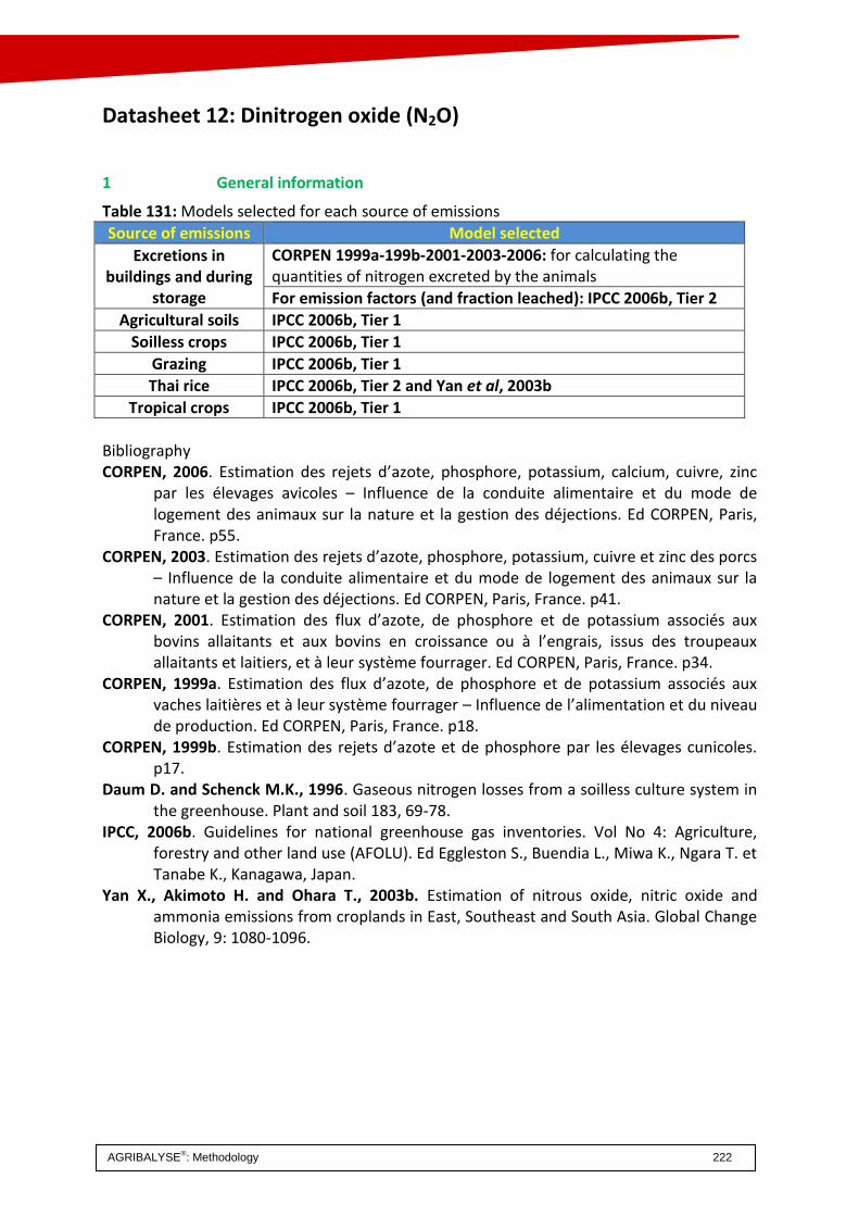
AGRIBALYSE®: Methodology 222
Datasheet 12: Dinitrogen oxide (N2O)
1 General information
Table 131: Models selected for each source of emissions
Source of emissions Model selected
Excretions in buildings and during
storage
CORPEN 1999a-199b-2001-2003-2006: for calculating the quantities of nitrogen excreted by the animals
For emission factors (and fraction leached): IPCC 2006b, Tier 2
Agricultural soils IPCC 2006b, Tier 1
Soilless crops IPCC 2006b, Tier 1
Grazing IPCC 2006b, Tier 1
Thai rice IPCC 2006b, Tier 2 and Yan et al, 2003b
Tropical crops IPCC 2006b, Tier 1
Bibliography CORPEN, 2006. Estimation des rejets d’azote, phosphore, potassium, calcium, cuivre, zinc
par les élevages avicoles – Influence de la conduite alimentaire et du mode de logement des animaux sur la nature et la gestion des déjections. Ed CORPEN, Paris, France. p55.
CORPEN, 2003. Estimation des rejets d’azote, phosphore, potassium, cuivre et zinc des porcs – Influence de la conduite alimentaire et du mode de logement des animaux sur la nature et la gestion des déjections. Ed CORPEN, Paris, France. p41.
CORPEN, 2001. Estimation des flux d’azote, de phosphore et de potassium associés aux bovins allaitants et aux bovins en croissance ou à l’engrais, issus des troupeaux allaitants et laitiers, et à leur système fourrager. Ed CORPEN, Paris, France. p34.
CORPEN, 1999a. Estimation des flux d’azote, de phosphore et de potassium associés aux vaches laitières et à leur système fourrager – Influence de l’alimentation et du niveau de production. Ed CORPEN, Paris, France. p18.
CORPEN, 1999b. Estimation des rejets d’azote et de phosphore par les élevages cunicoles. p17.
Daum D. and Schenck M.K., 1996. Gaseous nitrogen losses from a soilless culture system in the greenhouse. Plant and soil 183, 69-78.
IPCC, 2006b. Guidelines for national greenhouse gas inventories. Vol No 4: Agriculture, forestry and other land use (AFOLU). Ed Eggleston S., Buendia L., Miwa K., Ngara T. et Tanabe K., Kanagawa, Japan.
Yan X., Akimoto H. and Ohara T., 2003b. Estimation of nitrous oxide, nitric oxide and ammonia emissions from croplands in East, Southeast and South Asia. Global Change Biology, 9: 1080-1096.

AGRIBALYSE®: Methodology 223
2 Parameters for livestock production: excretions in buildings and during
storage
The quantities excreted were calculated using equations in CORPEN (1999a, 1999b, 2001, 2003, 2006). The emission factors depended on the storage system. The factors given in Table 132 were used to calculate the N2O emissions. Table 132: N2O emission factors depending on the excretion management system
AGRIBALYSE system IPCC system EF3 N2O
kg N2O-N per kg N excreted-
Covered slurry pit with natural crust liquid/slurry, with natural crust cover 0.005
Covered slurry pit without natural crust
liquid/slurry, without natural crust cover 0
Non-covered slurry pit with natural crust
liquid/slurry, with natural crust cover 0.005
Non-covered slurry pit without natural crust
liquid/slurry, without natural crust cover 0
Covered manure heap solid storage 0.005
Non-covered manure heap solid storage 0.005
Pig manure with straw solid storage 0.007
3 Parameters for plant production: agricultural soils
Figure 18 gives an overview of direct and indirect N2O emissions for plant production. Only the emission factors (flows and figures in red) were used: the other flows (amendments, volatilization – in yellow – and leaching – in blue) were calculated by the ammonia, nitrate and nitric oxide models using data collected for each crop.
Figure 18: N2O emissions model according to IPCC (2006b) tier 1.
IPCC tier 1 method (2006) Emission factors
N amendment
Res: 0% Min: 10% [2-20%] Org: 20% [5-5%] 1% [0.2-5%]
1% [0.3-3%]
0.75% [0.05-2.5%]
Cultivated plot

AGRIBALYSE®: Methodology 224
The N2O calculation model only uses IPCC (2006b) Tier 1 for the emission factors (EF1, EF4 and EF5, see equations 1 to 3 below). Equation n°1: Direct N2O emissions from managed soils (tier 1):
𝑁 − 𝑁2𝑂𝐷𝑖𝑟𝑒𝑐𝑡 = 𝑁 − 𝑁2𝑂𝑁𝐼𝑛𝑝𝑢𝑡𝑠+ 𝑁 − 𝑁2𝑂𝑂𝑆 + 𝑁 − 𝑁2𝑂𝑃𝑅
Given that: 𝑁 − 𝑁2𝑂𝑁𝐼𝑛𝑝𝑢𝑡𝑠
𝑖𝑠 [(𝐹𝑀𝑁 + 𝐹𝑂𝑁 + 𝐹𝐶𝑅 + 𝐹𝑀𝑁𝐶) × 𝐸𝐹1]
+ [(𝐹𝑀𝑁 + 𝐹𝑂𝑁 + 𝐹𝐶𝑅 + 𝐹𝑀𝑁𝐶)𝑅𝐼 × 𝐸𝐹1𝑅𝐼] 𝑁 − 𝑁2𝑂𝑂𝑆 𝑖𝑠 (𝐹𝑂𝑆,𝐶𝑀,𝑇𝑒𝑚𝑝 × 𝐸𝐹2𝐶𝑀,𝑇𝑒𝑚𝑝) + (𝐹𝑂𝑆,𝐶𝑀,𝑇𝑟𝑜𝑝 × 𝐸𝐹2,𝐶𝑀,𝑇𝑟𝑜𝑝)
+ (𝐹𝑂𝑆,𝐹,𝑇𝑒𝑚𝑝,𝑅𝑁 × 𝐸𝐹2,𝐹,𝑇𝑒𝑚𝑝,𝑅𝑁)
+ (𝐹𝑂𝑆,𝐹,𝑇𝑒𝑚𝑝,𝑃𝑁 × 𝐸𝐹2,𝐹,𝑇𝑒𝑚𝑝,𝑃𝑁 + (𝐹𝑂𝑆,𝐹,𝑇𝑟𝑜𝑝 × 𝐸𝐹2,𝑇𝑟𝑜𝑝))
𝑁 − 𝑁2𝑂𝑃𝑅𝑖𝑠 (𝐹𝑃𝑅,𝐶𝑃𝑆 × 𝐸𝐹3𝑃𝑅,𝐶𝑃𝑆) + (𝐹𝑃𝑅,𝑆𝐴 × 𝐸𝐹3𝑃𝑅,𝑆𝐴)
Where:
N-N2ODirect is the direct annual N-N2O emissions for managed soils, kg N-N2O yr-1 N-N2ON Inputs is the direct annual N-N2O emissions from N inputs to managed soils, kg
N-N2O yr-1 N-N2OOS is the direct annual N-N2O emissions for managed organic soils, kg N-N2O yr-1 N-N2OPR is the direct annual N-N2O emissions for urine and feces inputs to land used
for pasture and outdoor runs, kg N-N2O yr-1 FMN is the annual quantity of mineral N fertilizer applied to the soil, kg N yr-1 FON is the annual quantity of animal manure, compost, sludge and other organic N
amendment applied to the soil (Note: if sludge is included, cross check with the Waste LCI data sets to avoid double accounting of N2O emissions from N in the sludge), kg N yrn-1
FCR is the annual quantity of N returned to the soil in crop residues (air and underground), including nitrogen fixing crops and reseeding of forage/meadows, kg N yr-1
FMNC is the annual quantity of mineralized N in the mineral soils from loss of carbon from soil organic matter owing to changes in land use or land management, kg N yr-1
FOS is the annual area of organic soils drained/managed, ha (Note: the additional subscripts CM, F, Temp, Trop, RN and PN refer to cultivated land and meadows, forests, temperate, tropical, rich in nutrients and poor in nutrients, respectively)
FPR is the annual quantity of N from urine and feces deposited by the animals grazing in the meadows and outdoor runs, kg N yr-1 (Note: the additional subscripts CPS and SA refer to cattle, poultry and swine, and sheep and other animals, respectively)
EF1 is the N2O emission factor for N inputs, kg N-N2O (kg N inputs)-1 EF1RI is the N2O emission factor for N inputs to flooded rice, kg N-N2O (kg N inputs)-1 EF2 = is the N2O emission factor for N inputs for drained/managed organic soils, kg N-
N2O ha-1.yr-1 (Note: the subscripted indices CM, F, Temp, Trop, RN and PN refer to cultivated land and meadows, forests, temperate, tropical, rich in nutrients and poor in nutrients, respectively)

AGRIBALYSE®: Methodology 225
EF3PR is the N2O emission factor for urine and feces deposited by the animals grazing in meadows and outdoor runs, kg N yr-1 (Note: the subscripted indices CPS and SA refer to cattle, poultry and swine, and sheep and other animals, respectively)
Equation n°2: N2O emissions from the airborne deposition of volatized nitrogen from soil management (tier 1):
𝑁 − 𝑁2𝑂(𝐴𝐷) = [(𝐹𝑀𝑁 × 𝐹𝑟𝑎𝑐𝐺𝐴𝑆𝐹) + ((𝐹𝑂𝑁 + 𝐹𝑃𝑅) × 𝐹𝑟𝑎𝑐𝐺𝐴𝑆𝑂)] × 𝐸𝐹4
Where:
N-N2O(AD) is the annual quantity of N-N2O produced by airborne deposition of N volatilized from managed soils, kg N2O–N yr-1
FMN is the annual quantity of mineral N fertilizer applied to the soil, kg N yr-1 FracGASF is the fraction of mineral N fertilizer volatilized in the form of NH3 and NOx, kg
N volatilized (kg of N applied)-1 FON is the annual quantity of managed animal manure, compost, sludge and other
organic N amendments applied to the soil, kg N yr-1 FPR is the annual quantity of N from urine and feces deposited by animals grazing in the
meadows, outdoor runs and plots, kg N yr-1 FracGASO is the fraction of the organic N fertilizer materials applied (FON) plus the N
from urine and feces deposited by grazing animals (FPR) volatilized in the form of NH3 and NOx, kg N volatilized (kg of N applied or deposited)-1
EF4 is the N2O emission factor for airborne deposition of N on the soil and aquatic surfaces, [kg N-N2O (kg N-NH3 + N-NOx volatilized)-1]
Equation n°3: N2O emissions from nitrogen leached from managed soil, in regions with leaching and runoff (tier 1):
𝑁 − 𝑁2𝑂(𝐿) = (𝐹𝑀𝑁 + 𝐹𝑂𝑁 + 𝐹𝑃𝑅 + 𝐹𝐶𝑅 + 𝐹𝑀𝑁𝐶) × 𝐹𝑟𝑎𝑐𝐿𝐸𝐴𝐶𝐻−(𝐻) × 𝐸𝐹5
Where:
N-N2O(L) is the annual quantity of N-N2O produced by leaching and runoff after adding N to managed soils in regions with leaching and runoff, kg N-N2O yr-1
FMN is the annual quantity of mineral N fertilizer applied to the soil in regions with leaching and runoff, kg N yr-1
FON is the annual quantity of managed animal manure, compost, sludge and other organic N amendments applied to the soil in regions with leaching and runoff, kg N yr-1
FPR is the annual quantity of N from urine and feces deposited by animals grazing in meadows and outdoor runs in regions with leaching and runoff, kg N yr-1
FCR is the annual quantity of N returned to the soil in crop residues (airborne and underground), including nitrogen fixing crops, and reseeding of forage/meadows in regions with leaching and runoff, kg N yr-1
FMNC is the annual quantity of mineralized N in mineral soils, from loss of carbon from soil organic matter owing to changes in land use and land management in regions with leaching and runoff, kg N yr-1

AGRIBALYSE®: Methodology 226
FracLEACH-(H) is the fraction of all the N mineralized/added to managed soil in regions with leaching and runoffs and lost by leaching and runoff, kg N (kg of added N)-1
EF5 is the N2O emission factor for N losses owing to leaching and runoff, kg N-N2O (kg of N leached or runoff)-1
To calculate the leached (NO3) and volatilized (NH3) fractions, this model used the quantities calculated in the nitrate and ammonia models. The quantity of nitrogen considered includes the quantity of organic and mineral manure as well as the airborne and underground parts of crop residues (data defined in the data collection model) To be consistent with the decision not to take account of changes in soil carbon stocks, account was not taken of N2O emissions from mineralization of nitrogen caused by losses of organic matter caused by land use changes. This approach was applied to all production systems for plants, annual crops, orchards, grapevines, meadows and soilless crops.
4 Parameters for plant production: grazing
For direct N2O emissions from grazing, Tier 1 of the IPCC (2006b) model was applied without modification, using factors EF3PRPCPP (20% for cattle, pigs and poultry) and EF3PRPSO (10% for sheep, etc) depending on the type of animal grazing (this was defined for LCI data sets for grass grazed by one cow, and so a factor of 20% was applied). The leached and volatized fractions, required to calculate indirect emissions, were determined using the nitrate and ammonia calculation models.
5 Parameters for plant production: calculating N returned to the soil from
reseeding of meadows (FCR)
The quantity of nitrogen returned to the soil from the reseeding of forage/meadows (included in FCR, cf. equation 3 above) was calculated by applying formula 11.6 of IPCC (2006b), page 11.14ff and using the default values given in Table 11.2 of the IPCC (2006b) report. For permanent meadows, the annual reseeding was set at 0 (cf. column 3 of Table 133) which means that account was not taken of N returned to the soil. Table 133 gives the quantities of nitrogen returned to the soil on reseeding of forage/meadows for AGRIBALYSE LCI data sets.

AGRIBALYSE®: Methodology 227
Table 133: Quantities of nitrogen returned to the soil on reseeding of forage/meadows for AGRIBALYSE LCI data sets
LCI data set / crop Name of crop in Table 11.2 of IPCC (2006a)
% of area renewed each year
Nitrogen returned (kg N/(ha*yr)
Grazed grass, permanent meadow, without clover, Auvergne
perennial grass 0 0
Baled grass, permanent meadow, without clover, Auvergne
perennial grass 0 0
Grass silage, horizontal silo, permanent meadow, without clover, Auvergne
perennial grass 0 0
Baled hay, permanent meadow, without clover, Auvergne,
perennial grass 0 0
Grazed grass, permanent meadow, without clover, Northwestern region
perennial grasses 0 0
Baled grass, permanent meadow, without clover, Northwestern region
perennial grasses 0 0
Grazed grass, temporary meadow, without clover, Northwestern region,
perennial grasses 0 0
Grazed grass, temporary meadow, without clover, Northwestern region
non n fixing forages 0.25 10.79
Baled grass, temporary meadow, without clover, Northwestern region
non n fixing forages 0.25 14.12
Baled hay, temporary meadow, without clover, Northwestern region
non n fixing forages 0.25 15.61
Grazed grass, permanent meadow, with clover, Northwestern region
perennial grass 0 0
Baled grass, temporary meadow, with clover, Northwestern region
perennial grass 0 0
Baled hay, permanent meadow, with clover, Northwestern region
perennial grass 0 0
Grazed grass, temporary meadow, with clover, Northwestern region
grass clover mixtures 0.25 18.99
Baled grass, temporary meadow, with clover, Northwestern region
grass clover mixtures 0.25 26.84
Grass silage, horizontal silo, temporary meadow, with clover, Northwestern region
grass clover mixtures 0.25 25.23
Baled hay, temporary meadow, with clover, Northwestern region
grass clover mixtures 0.25 29.31
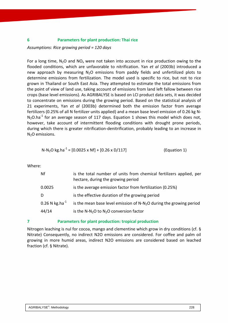
AGRIBALYSE®: Methodology 228
6 Parameters for plant production: Thai rice
Assumptions: Rice growing period = 120 days
For a long time, N2O and NOx were not taken into account in rice production owing to the flooded conditions, which are unfavorable to nitrification. Yan et al (2003b) introduced a new approach by measuring N2O emissions from paddy fields and unfertilized plots to determine emissions from fertilization. The model used is specific to rice, but not to rice grown in Thailand or South East Asia. They attempted to estimate the total emissions from the point of view of land use, taking account of emissions from land left fallow between rice crops (base level emissions). As AGRIBALYSE is based on LCI product data sets, it was decided to concentrate on emissions during the growing period. Based on the statistical analysis of 21 experiments, Yan et al (2003b) determined both the emission factor from average fertilizers (0.25% of all N fertilizer units applied) and a mean base level emission of 0.26 kg N-N2O.ha-1 for an average season of 117 days. Equation 1 shows this model which does not, however, take account of intermittent flooding conditions with drought prone periods, during which there is greater nitrification-denitrification, probably leading to an increase in N2O emissions.
N-N2O kg.ha-1 = [0.0025 x Nf] + [0.26 x D/117] (Equation 1)
Where:
Nf is the total number of units from chemical fertilizers applied, per hectare, during the growing period
0.0025 is the average emission factor from fertilization (0.25%)
D is the effective duration of the growing period
0.26 N kg.ha-1 is the mean base level emission of N-N2O during the growing period
44/14 is the N-N2O to N2O conversion factor
7 Parameters for plant production: tropical production
Nitrogen leaching is nul for cocoa, mango and clementine which grow in dry conditions (cf. § Nitrate) Consequently, no indirect N2O emissions are considered. For coffee and palm oil growing in more humid areas, indirect N2O emissions are considered based on leached fraction (cf. § Nitrate).

AGRIBALYSE®: Methodology 229
Datasheet 13: Active substances in pesticides
1 General information
Table 134: Models selected for each source of emissions
Source of emissions Model selected
All crops ecoinvent v2 (Nemecek and Kägi, 2007)
Thai rice Expertise S. Perret (CIRAD)
Soilless crops This report
Soil under plastic film This report
Bibliography Nemecek T. and Kägi T., 2007. Life Cycle Inventories of Swiss and European Agricultural
Production Systems - Data v2.0 (2007). Ecoinvent report No. 15a. Ed Swiss Center for Life Cycle Inventories, Zurich and Dübendorf, Switzerland. p360.
2 Parameters for plant production: all crops
It was assumed that 100% of active substances applied were transferred to the soil. This method ensured comparability with databases such as ecoinvent. However, this approach only quantifies maximum possible emissions.
3 Parameters for plant production: soilless crops and special production
systems
As there was no precise information on the distribution and fate of active substances in systems where the soil was protected (eg. soil covered with a mulching film or in greenhouses or tunnels) and for soilless crops, it was taken that 100% of the flows were ending into the soil.

AGRIBALYSE®: Methodology 230
4 Parameters for plant production: Thai rice
It was assumed that 100% of active substances were transferred to the soil and water compartments as they are not thought to concentrate in the rice grains or remain in the plots after harvest. In production zones, most of the pesticides used were insecticides, which were applied to the crop by hand at various stages when the paddy fields were flooded most of the time. In this conditions, it was, therefore, decided to split the emissions equally between the soil and the water (50% - 50%).
Table 135 gives the various approaches selected.
Table 135: Allocation of emissions from active substances in pesticides between the air, water and agricultural soil compartments
Compartment
Crop / production system Air Water Agricultural soil
All crops (with the following exceptions) 100%
Soilless
100%
Rice 50% 50%
Soil under plastic film 100%

AGRIBALYSE®: Methodology 231
Datasheet 14: Emissions from fish farms
1 General information
Table 136: Models selected for each source of emissions
Source of emissions Model selected
Nitrogen Papatryphon et al, 2005
Phosphorus Papatryphon et al, 2005
Total suspended solids (TSS) Papatryphon et al, 2005
N, P and TSS emissions from fish farms are considered separately because the emission mechanisms involved are significantly different from other livestock production systems. General principle of the model The model selected is based on a mass balance for inputs and outputs which requires a knowledge of the composition of the feed rations distributed to the animals, the biochemical composition of the fish and the quantity of undigested nutrients. Bibliography Papatryphon E., Petit J., van der Werf HMG., Kaushik S. and Kanyarushoki C., 2005.
Nutrient-balance modeling as a tool for environmental management in aquaculture: The case of trout farming in France. Environmental Management 35 (2), 161-174.
2 Parameters: nitrogen losses
Equation (1) below was used. Ntotal waste = Ns + Ni Eq (1)
Nf = [(Ad – (Ad x % Anc)) x (% protein / 6.25)] x (100 – ADC)% Nnc = Ad x % Anc x (% protein / 6.25) Ns = Nf + Nnc Ng = (Ad x TN) / CI Ni = Nc – Nf - Ng N-NH4 = Ni x 0.8 NH4 = N-NH4 x 1.26 Ndissolved = Ni – N-NH4 Where: Ad is the feed distributed % Anc is the percentage of feed not consumed, estimated at 5% % protein is the percentage of raw protein in the feed ADC is the Apparent Digestibility Coefficient, estimated at 90% (±5%) Nc is the nitrogen consumed Nd is the nitrogen digested
Nf is the fecal nitrogen Ni is the dissolved nitrogen TN is the nitrogen content of the fish (0.0256 to 0.0272 gN/g body mass) Ng is the nitrogen content in the body mass increase N-NH4 is nitrogen in the form of ammonia CI is the consumption index

AGRIBALYSE®: Methodology 232
3 Parameters: phosphorus losses
Equation (2) below was used: Ptotal waste = Ps + Pi Eq (2)
Where: Pf = [(Ad – (Ad x % Anc)) x (% P)] x (100 – ADC) % Nnc = Ad x % Anc x 90% x (% P / 90%) Ps = Pf + Pnc Pg = (Ad x 0.0045) / CI Pi = Pc – Pf - Pg Where: Ad is the feed distributed % Anc is the percentage of feed not consumed, estimated at 5% % P is the percentage of phosphorus in the feed ADC is the Apparent Digestibility Coefficient, estimated at 50% (±10%) Pc is the phosphorus consumed
Pd is the phosphorus digested Pf is the fecal phosphorus Pi is the dissolved phosphorus Pg is the phosphorus content in the body weight increase, based on the P content of the fish body (0.40 to 0.45 gP/100 g body mass) CI is the consumption index
4 Parameters: TSS
Equation (3) below was used: TSStotal waste = TSSf + TSSnc Eq (3)
TSSf = {[(Ad – (Ad x %Anc)] x ∑ [% nutrient x (100 – ADC)%]} ∑ [% nutrient x (100 – ADC) %] = (% proteins x (100 – ADC)%) + (% lipids x (100 – ADC)%) + (%
carbohydrates x (100 – ADC)%) + (% fiber x (100 – ADC)%) + (% ash x (100 – ADC)%)
TSSnc = (Ad x %Anc x % dry matter) Where: Ad is the feed distributed % Anc is the percentage of feed not consumed, estimated at 5% % protein is the percentage of protein in the feed % lipids is the percentage of lipids in the feed % carbohydrates is the percentage of carbohydrates in the feed
% fiber is the percentage of fiber in the feed % ash is the percentage of ash in the feed ADC is the Apparent Digestibility Coefficient, estimated at 50% (±10%) % dry matter is the percentage of dry matter in the feed

AGRIBALYSE®: Methodology 233
Datasheet 15: Extrapolation of seed and plant LCI data sets
1. General information
The seed LCI data sets were extrapolated for crops documented in GESTIM (Gac et al, 2010).
a) by recalculating the quantity of seed produced at the exit from the production site (taking account of losses)
b) by calculating an extrapolation factor based on a comparison of energy consumption according to GESTIM and data collected for the AGRIBALYSE program
c) by adding the transport and energy requirements for seed production given in GESTIM. As some of the losses are reused, these additional inputs were allocated by mass.
2. Parameters
Calculating the quantity produced. The quantity of seeds produced was calculated using the following formula. QSP = (RSC * (1 - tR)) * (1 – tL) Where: QSP is the quantity of seeds produced, at exit rather than on production RSC is the gross seed yield, at the farm gate tR is the reuse rate tL is the loss rate on the production site

AGRIBALYSE®: Methodology 234
The data for these parameters were taken from GESTIM (Table 137).
Table 137: Yield and loss/reject rates according to GESTIM (Gac et al, 2010)
Crop Yield
RSC (kg/ha) Reject rate
tR (%) Reuse tRR (%)
Loss rate tL (%)
Reuse tRL (%)
Sugar beet 2038 0.54 0 87 0
Durum wheat 3514 1.91 100 15 80
Soft wheat 4360 2.54 95 15 80
Rapeseed 1546 4.00 0 16 80
Alfalfa 2955 2.02 0 10 80
Maize 2790 0.59 0 12 80
Barley 4400 2.05 0 15 80
Protein peas 2955 0.33 0 10 80
Potatoes 24840 3.51 0 13 100
Starch potatoes 24840 3.51 0 13 100
Rye 4400 1.06 0 15 80
Sorghum grain 2170 3.27 0 12 80
Sunflowers 937 1.70 0 10 80
Triticale 3509 2.47 0 15 80
Other (average)
3 0 15 0
If the LCI seed data set was extrapolated for a crop not listed in GESTIM (eg: carrots), the yield at the farm gate was estimated based on expert opinion. Average values were used for the loss and reject rates (Table 137, row “Other”). Calculating the extrapolation factor to extrapolate the LCI seed data set from the LCI data set for a given crop. Table 130 gives the electricity and fuel consumptions taken into account for the production at the farm gate.
Table 138: Electricity and fuel consumption for seed production according to GESTIM (Gac et al, 2010)
Crop Electricity Fuel
kWh/ha l/ha
Sugar beet 1500 204
Durum wheat 9 99
Soft wheat 52 92
Rapeseed 0 90
Maize 1545 159
Barley 16 103
Protein peas 48 102
Potatoes 50 267
Starch potatoes 53 267
Rye
86
Sunflowers 500 84
Triticale 14 89
Other 344.2 136.8

AGRIBALYSE®: Methodology 235
If the LCI seed data set was extrapolated for a crop not listed in GESTIM (eg: carrots), average consumptions were used (Table 138, row “Other”).
The extrapolation factor was calculated using the following formula.
𝑓𝐸𝑥 = max(𝐶𝐸𝑙𝐺
𝐶𝐸𝑙𝐴 ,𝐶𝐶𝑎𝐺
𝐶𝐶𝑎𝐴 , 1) ∗
𝑅𝑆𝑒𝑒𝑑
𝑅𝐶𝑟𝑜𝑝
Where: fEx is the extrapolation factor CElG is the electricity consumption according to GESTIM CElA is the electricity consumption according to AGRIBALYSE CCaG is the fuel consumption according to GESTIM CCaA is the fuel consumption according to AGRIBALYSE RSeed is the seed yield (kg/ha) RCrop is the crop yield (kg/ha) Each input used for producing the AGRIBALYSE crop was multiplied by this factor. Adding processes related to seed production. Table 139 gives the inputs required for seed production.
Table 139: Distances and means of transport and energy consumption for seed production
Distances and means of transport (km) Energy consumption
Crop Field site Site farm Electricity Natural gas
Agricultural trailer Lorry Lorry kWh/t MJ/t
Sugar beet
1000 800
Durum wheat 15
230 20
Soft wheat 15
230 20
Rapeseed 15
230 20
Alfalfa 15
230 20
Maize 15
230 40 681.12
Barley 15
230 20
Protein peas 15
230 20
Potatoes
15 305 37
Starch potatoes
15 305 20
Rye 15
230 20
Sorghum grain 15
230 20
Sunflowers 15
230 20
Triticale 15
230 20
Other
15 305 20
These inputs were multiplied by the quantity of certified seed (RCS * (1 - tR)), and allocated to the quantity of seed produced (QSP) and the losses reused using an allocation factor (fAlL), calculated using the following formula. fAlL = ( ( tR x tRR ) + ( (1 – tR )x tL x tRL )

AGRIBALYSE®: Methodology 236
Where fAlS is 1 - fAlL
fAlL is the reused losses allocation factor fAlS is the seed allocation factor tRR is the reject reuse rate tRL is the loss reuse rate on the production site The quantities of energy consumed (fuel and electricity) were adjusted by subtracting the AGRIBALYSE crop energy from the GESTIM crop energy so that they were the same as those given in Table 138.
Table 140 : LCIs used for commercial seeds
Seed LCI name Type Used for
Carrot seed, conventional, at farm gate extrapolation All carots in conventional production
Carrot seed, organic, at farm gate extrapolation Organic carots
clover seed ip, at regional storehouse LCI ecoinvent alfalfa
Durum wheat seed, conventional, national average, at farm gate extrapolation Hard wheat
Grain maize seed, conventional, national average, at farm gate extrapolation Grain and forrage maize
Grass seed IP, at regional storehouse LCI ecoinvent Grass, hay, pastures, grass in vineyards
Rapeseed, seed, conventional, at farm gate extrapolation rapeseed
Soft wheat seed, conventional, breadmaking quality, 15% moisture, at farm gate extrapolation All soft wheats in conventionnal
Spring barley seed, conventional, malting quality, national average, at farm gate extrapolation All barleys (forage and malt)
Spring pea seed, conventional, at farm gate extrapolation Spring pea
Starch potato seed, conventional, national average, at farm gate extrapolation Startch potato
Sugar beet seed, conventional, at farm gate extrapolation Sugarbeet rhizom
Sunflower, seed, conventional, 9% moisture, national average, at farm gate extrapolation sunflower
Triticale seed, conventional, national average, at farm gate extrapolation triticale conventionnal
Ware potato seed, conventional, at farm gate extrapolation Ware potatoes for fresh market
Winter pea seed, conventional, 15% moisture, at farm gate extrapolation Winter pea

AGRIBALYSE®: Methodology 237
Datasheet 16: Use of “Animal of 0 day” LCIs for initiating animal
systems Animal systems must be initiated by an “animal input”, incorporating impacts related to reproduction and gestation. Those impacts depends on the allocation rule between dam/milk/calf. Here are given each “animal input” used for system initiation. Then, all the other animal growth stages are added for building the “final product”.
Table 141 : Animal classes initiating animal production systems.
System For the products coming from… the LCI … was used for initiating the animal system.
Beef production
101 Conventional lowland milk system, silage maize more than 30%
Calf of 0 day, conventional, lowland milk system,silage maize more than 30% (animal class), at farm gate
102 Conventional lowland milk system, silage maize 10 to 30%
Calf of 0 day, conventional, lowland milk system,silage maize 10 to 30% (animal class), at farm gate
103 Conventional lowland milk system, silage maize 5 to 10%
Calf of 0 day, conventional, lowland milk system,silage maize 5 to 10% (animal class), at farm gate
104 Organic lowland milk system, silage maize 5 to 10%
Calf of 0 day, organic, lowland milk system,silage maize 5 to 10% (animal class), at farm gate
105 Conventional highland milk system, grass fed Calf of 0 day, conventional, highland milk system,grass fed (animal class), at farm gate
106 Conventional lowland beef fattening farm Conventional lowland milk system, silage maize more than 30%, animal class 1, at farm
110 Conventional suckler cow system, more than 1.2 LU per ha
Calf of 0 day, conventional, suckler cow system,more than 1.2 LU per ha (animal class), at farm gate
108 Conventional suckler beef fattening farm (heifers), more than 1.2 LU per ha
Conventional suckler cow system, more than 1.2 LU per ha, animal class 1, at farm
109 Conventional suckler beef fattening farm (bulls), more than 1.2 LU per ha
Conventional suckler cow system, more than 1.2 LU per ha, animal class 1, at farm
107 Conventional suckler cow system, less than 1.2 LU per ha
Calf of 0 day, conventional, suckler cow system,less than 1.2 LU per ha (animal class), at farm gate
111 Conventional suckler beef fattening farm (bulls), less than 1.2 LU per ha
Conventional suckler cow system, less than 1.2 LU per ha, animal class 1, at farm
112 Conventional beef calf fattening system Conventional lowland milk system, silage maize more than 30%, animal class 1, at farm
Sheep and goat production$

AGRIBALYSE®: Methodology 238
113 Conventional milk sheep farm, Roquefort system
Lamb of 0 day, conventional, Roquefort system (animal class), at farm gate
114 Conventional goat farm, intensive forage area
Kid goat of 0 day, conventional, intensive forage area (animal class), at farm gate
115 Conventional sheep farm, indoor system Lamb of 0 day, conventional, indoor production system (animal class), at farm gate
Pig production
132 Conventional porc production, fed rapeseed meal
Pig, conventional, fed rapeseed meal (animal class), at farm gate
133 Conventional porc production, fed soybean meal
Pig, conventional, fed soybean meal (animal class), at farm gate
134 Conventional porc production, on-farm feed supply
Pig, conventional, on-farm feed supply (animal class), at farm gate
135 Conventional porc production, excess slurry treatment
Pig, conventional, excess slurry treatment (animal class), at farm gate
136 Conventional porc production, national average
Pig, conventional, national average (animal class), at farm gate
137a Label Rouge porc production, with run system
Pig, Label Rouge, pig with run system (animal class), at farm gate
137b Label Rouge porc production, outdoor system
Pig, Label Rouge, outdoor system (animal class), at farm gate
139 Organic porc production Pig, organic (animal class), at farm gate

AGRIBALYSE®: Methodology 239
Datasheet 17: Allocation of P and K fertilizers and organic N fertilizer
within cropping sequences
1. General information
As described in chapter B.3.3, P and K fertilizers and organic N fertilizer were allocated to cropping sequences. In the AGRIBALYSE program, this allocation was implemented by “corrective flows” whereby the LCI data sets include: a) the inputs actually applied and entered in the data collection module b) the input corrections (difference between real flows and allocated flows) c) the emissions related to the inputs actually applied d) and the emission corrections for the input corrections (N2O, NH3, NO, phosphorus and trace metal emissions). This approach makes the allocation explicit. It is also required as the direct emissions calculation models need more precise data (see below).
2. Parameters
Table 142 gives the quantities of P and K fertilizers and organic N fertilizer applied to crops after allocating the shared inputs for the cropping sequence. These values were calculated using the method described in chapter B.3.3.
Table 142: Quantities of P and K fertilizer and organic N fertilizer after allocating the shared inputs for cropping sequences (Source: Arvalis, based on the 2006 survey on farming practices by the SSP)
Crop Quantity allocated
Mineral K (kg K2O/ha)
Total K % K2O org
Mineral P (kg P2O5/ha)
Total P (kg P2O5/ha)
Norg (kg N/ha)
Sugar beet 126 193 29 40 44
Durum wheat 18 22 36 40 4
Soft wheat 33 58 39 58 18
Organic soft wheat following faba beans
0 0 0 15 56
Organic soft wheat following alfalfa
0 0 0 20 6
Rapeseed 25 41 34 44 17
Faba beans 25 61 46 66 8
Organic faba beans 0 0 0 30 6
Forage maize 65 258 33 79 114
Grain maize 55 96 52 78 37
Barley, malting quality 34 59 38 52 15
Forage barley 34 59 38 52 15
Starch potatoes 161 259 25 37 43
Peas 41 63 26 33 9

AGRIBALYSE®: Methodology 240
Crop Quantity allocated
Mineral K (kg K2O/ha)
Total K % K2O org
Mineral P (kg P2O5/ha)
Total P (kg P2O5/ha)
Norg (kg N/ha)
Potatoes 161 259 25 37 43
Sunflowers 23 34 25 32 11
Triticale 35 86 26 48 28
Organic triticale 0 0 45 44
Calculating the input flow correction Four input flows were corrected using the following formula.
FCfert = FOfert – FRfert Where:
FCfert is the correction for the fertilizer fert (see below) FOfert is the original input of the fertilizer fert (set in the data collection module) FRfert is the allocated input of the fertilizer fert (see Table 142) fert is mineral K, mineral P, organic P or organic N
Table 142 is used to calculate the quantity of organic P fertilizer as the difference between total P and mineral P as well as to calculate the quantities of organic and mineral K2O fertilizer. As the form in which the mineral fertilizers will be applied is not known, the correction factors for mineral K and mineral P were included in the LCI data sets as average fertilizers (“average mineral fertilizer, as K2O, at regional storehouse/kg/FR” and “average mineral fertilizer, as P2O5, at regional storehouse/kg/FR”). Calculating the emission flow correction factor The four input flows were corrected by adjusting (positive or negative) the following emissions: a) Mineral PK fertilizer
Phosphate emissions by leaching or runoff (PK fertilizer) b) Organic N fertilizer
Ammonia emissions (NH3) Nitric oxide emissions (NO) Dinitrogen oxide emissions (N2O)
c) Mineral PK and organic N fertilizers Trace metal emissions
Account was not taken of nitrate leaching. The emission flow correction was calculated on the basis of the particular direct emission calculation models. a) Effects on phosphorus emissions To estimate the effect of allocation on phosphorus emissions, it is necessary to know the quantities of phosphorus applied in: i) organic liquid, ii) organic solid and iii) mineral form. The quantity of organic phosphorus allocated according to Table 128 was allocated between solid and liquid forms depending on the organic phosphorus fertilizer actually applied. If no organic

AGRIBALYSE®: Methodology 241
fertilizer was applied to the crop, the allocation between solid and liquid forms was based on the composition of the average French organic manure for phosphorus amendment (Table 151). Separate factors FCLB and FC were defined (see phosphorus model, datasheet 11), depending on the form of the amendment, and the quantities of phosphorus lost by leaching or runoff were calculated after allocation. The final corrected flows, added to the LCI data sets, were the difference between the flows without allocation and the flows after allocation:
CFPR/L = FOPR/L – FRPR/L Where:
CFPR/L is the correction factor for phosphorus lost by runoff / leaching FOPR/L is the original flow for phosphorus lost by runoff / leaching FRPR/L is the flow for phosphorus lost by runoff / leaching after allocation
b) Effects on ammonia (NH3) and nitric oxide (NO) emissions The type of manure applied (cattle slurry, pig slurry, etc., see datasheets 1 and 10) must be known in order to calculate NH3 emissions. An average organic manure was defined for the calculation (Table 143) assuming that each kilogram of organic nitrogen applied produced an emission of 147 g of N-NH3 (NH3AvgOrg).

AGRIBALYSE®: Methodology 242
Table 143: Composition of average organic French manure (Source: Arvalis, based on the survey on farming practices 2006 of SPP) and calculation of the average NH3 emissions per kg average organic manure
Manure Form % (for N) %
attributable TAN
%EF NH3
N-NH3 (kg N/kg N)
% (for P)
form
Cattle manure Average cattle manure 64.47 68.84 0.19 0.79 1.05E-01 46 farm solid
Dry layer droppings Dry poultry droppings 4.16 4.45 0.10 0.69 3.22E-03 8 farm solid
Broiler manure Broiler manure 4.07 4.34 0.17 0.79 5.87E-03 12 farm solid
Compost from animals Straw rich cattle manure compost 3.34 3.57 0.05 0.71 1.27E-03 2 farm solid
Vinasse Concentrated sugar beet vinasse 3.03 3.23 0.10 0.81 2.62E-03 0 sundry liquid
Sheep manure Sheep manure 2.82 3.01 0.10 0.90 2.71E-03 2 farm solid
Sludge Sludge 2.79 2.98 0.71 0.40 8.46E-03 5 sundry liquid
Green waste compost Green waste compost 2.66 2.84 0.10 0.71 2.12E-03 1 compost solid
Other food industry sludge 2.55 3
Pig slurry Mixed pig slurry 2.34 2.50 0.71 0.40 7.15E-03 7 farm liquid
Cattle slurry Undiluted cattle slurry 1.84 1.96 0.50 0.55 5.39E-03 2 farm liquid
Other industrial sludge 1.47 2
Laying hen slurry 1.27 3
Other effluent 0.83 1
Rabbit slurry Rabbit slurry 0.74 0.79 0.07 0.51 2.64E-04 2 farm liquid
Pig manure Straw rich pig manure 0.70 0.75 0.32 0.81 1.93E-03 1 farm solid
Duck manure Manure from ducks ready for force feeding
0.29 0.31 0.30 0.71 6.71E-04 1 farm solid
Household waste compost Household waste compost 0.26 0.28 0.10 0.71 2.08E-04 0 compost solid
Semi solid poultry droppings 0.18 1
Sugar scum Sugar scum 0.10 0.11 0.10 0.81 8.92E-05 1 sundry liquids
Sheep slurry 0.06 0
Calf slurry Beef calf slurry 0.02 0.02 0.84 0.55 1.08E-04 0 farm liquid
Total 100.0 0.147 100
Total attributable 93.64
This average fertilizer can be used to calculate the NH3 emission flow correction directly by multiplying this factor by the quantity of organic N allocated:
NH3 = NH3AvgOrg x CFNorganic Where:
NH3 is the NH3 emission flow correction
FCNorganic is the correction for organic N NH3AvgOrg is the NH3 emissions per kg average organic N (calculated using Table 143)
The same approach was used for NO emissions using an average emission factor of 0.026.

AGRIBALYSE®: Methodology 243
c) Effects on dinitrogen oxide emissions (N2O) Allocating the quantity of organic nitrogen also affects the direct and indirect emission of dinitrogen oxide:
- The direct N2O emissions are calculated by applying the emission factor to the corrected
flow of organic nitrogen.
- The corrected flows for indirect N2O emissions due to the volatilization of NH3 and NOx are
calculated by applying the emission factors to the corrected NH3 and NOx flows
N2Odir = CFNorg x EF1
N2Oindir = (NH3 + NOx) x EF4
Where:
N2Odir is the correction for direct N2O emissions
N2Oindir is the correction for indirect N2O emissions
FCNorg is the correction for the organic nitrogen input
NH3 is the correction for NH3 emissions
NOx is the correction for NOx emissions EF1 is emission factor 1 (for direct emissions, see N2O model) EF4 is emission factor 4 (for indirect emissions, see N2O model)
d) Effects on trace metal emissions The allocation of organic PK and organic N affects trace metal flows by 1. Increasing (or decreasing) the trace metals leached or in runoff by adjusting the output flow
allocation factor (Allocx see datasheet 4, Figure 15) 2. Increasing (or decreasing) the trace metal flows into the soil depending on the quantity of
fertilizer allocated To calculate these effects, it is necessary to know how the input trace metal flows from the fertilizer have been allocated:
INx = CFy x Tyx
Where:INx is the corrected input flows of TMx (x = Cd, Cu, Zn, Pb, Ni, Cr or Hg) Tyx
is the trace metal content TMx (x = Cd, Cu, Zn, Pb, Ni, Cr or Hg) of the fertilizer allocated
(y = FCNorg, FCPMin and FCKMin)
CFy is the flow of fertilizer allocated (y = FCNorg, FCPMin and FCKMin) Average fertilizers were used to calculate the trace metal content of the fertilizers allocated (the quantity of nitrogen was used for the organic fertilizers allocated). The output flow allocation
factor can be calculated from the trace metal flows from the fertilizers allocated (INx).
Allocx’ = INx + DINx
(INx + DINx)+ Depx
Where: Allocx’ is the output flow allocation factor for trace metals after allocation INx is the initial trace metal input flow TMx

AGRIBALYSE®: Methodology 244
INx is the corrected trace metal input flow TMx Depx is the deposition of trace metals TMx (deposition from the air)
This data is used to calculate the effects on trace metal emissions.
LIx = LIx x (Allocx’ – Allocx)
RUx = RUx x (Allocx’ – Allocx)
SOx = INx Where:
LIx is the corrected flow for leached trace metals LIx is the quantity of trace metals leached before taking account of fertilizer allocation Allocx’ is the trace metal output flow allocation factor after allocation Allocx is the trace metal output flow allocation factor before taking account of fertilizer allocation
RUx is the corrected trace metal TMx flow lost by runoff/erosion RUx is the quantity of trace metal TMx lost by runoff/erosion before taking account of fertilizer allocation
INx is the corrected flow of trace metal TMx inputs
SOx is the corrected flow of TMx into the soil
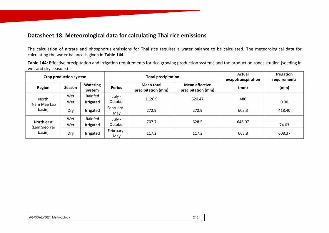
AGRIBALYSE®: Methodology 245
Datasheet 18: Meteorological data for calculating Thai rice emissions The calculation of nitrate and phosphorus emissions for Thai rice requires a water balance to be calculated. The meteorological data for calculating the water balance is given in Table 144.
Table 144: Effective precipitation and irrigation requirements for rice growing production systems and the production zones studied (seeding in wet and dry seasons)
Crop production system Total precipitation Actual
evapotranspiration Irrigation
requirements
Region Season Watering
system Period
Mean total precipitation (mm)
Mean effective precipitation (mm)
(mm) (mm)
North (Nam Mae Lao
basin)
Wet Rainfed July - October
1126.9 620.47 480 -
Wet Irrigated 0.00
Dry Irrigated February –
May 272.9 272.9 603.3 418.40
North east (Lam Sieo Yai
basin)
Wet Rainfed July - October
707.7 628.5 646.07 -
Wet Irrigated 74.03
Dry Irrigated February -
May 117.2 117.2 668.8 608.37

AGRIBALYSE: Methodology 246
Appendix E: Changes in soil carbon stocks
1 Introduction Taking account of the greenhouse gas flows was discussed at the seminar on selecting the calculation models to be used for direct emissions in AGRIBALYSE, which took place on May 19 and 20, 2011. Proposals were made for emissions of CH4, CO2 and N2O from agricultural production. However, it was decided that further consideration should be given to the issue of taking account of changes in soil carbon stocks.
The general brief for the AGRIBALYSE program stipulates that the methodology and deliverables of the program must conform to (among others) the JRC ILCD handbook. Regarding carbon storage, it states: “To take account of the emission or capture of greenhouse gases from or by the soil or land use change, account should be taken of the emission factors proposed by the IPCC, unless more specific data is available”. It was, therefore, recommended that the IPCC methodology for greenhouse gases and soil carbon storage should be used for drawing up LCAs. AGRIBALYSE does not aim to produce comparative LCAs, as for biofuels where a methodology is proposed to take account of land use change. The AGRIBALYSE program was designed to quantify the carbon flows from changes in the area of permanent meadows and other types of land use and changes in practices. The methodologies proposed for biofuels (European Commission, 2010) were, therefore, not considered to be very suitable.
Research The phenomenon of changes in soil carbon stocks under existing surfaces is well accepted and has been established by many studies. A. Benoist (2009) suggests that:
Stocks of organic matter including soil carbon depend on many parameters, in particular the climate, the nature of the soil and its use.
The levels of carbon stocks can be estimated using IPCC methods (2003). New methods were developed by A. Benoist to allow changes in soil carbon to be taken into account reversibly and slowly. However, these methods, which define the Global Warming Potential (GWP) are still not at a stage where they can be used easily in LCA software. Research has been carried out by the Institut de l’Elevage on carbon storage by meadows as a means of attenuating the effect of breeding livestock on the greenhouse effect. A working group was set up to determine how to take account of changes in soil carbon stocks. This group comprised the following persons, some of whom but not all were involved in the AGRIBALYSE program:
Anthony Benoist (CIRAD) Cécile Bessou (CIRAD) Jean-Baptiste Dollé (IDELE)

AGRIBALYSE: Methodology 247
Armelle Gac (IDELE) Etienne Mathias (CITEPA) Anne Paillier (ADEME) Thibault Salou (INRA) Aurélie Tailleur (ARVALIS) Hayo van der Werf (INRA)
The situations studied
Changes in soil carbon stocks are likely to be observed: during land use change (LUC) on existing agricultural land where it is caused by changes in cultivation practices
Changes in soil carbon stocks were not taken into account for products from overseas.
I- Soil carbon storage/release without land use change
Carbon is known to be stored in permanent meadows but the causes are not easy to identify. The cause may be a result of changing climate, which causes carbon sequestration owing to greater biomass, or of intensification in meadow management practices. For LCAs, only the effects of meadow management practices on carbon storage and the effect of crop management practices on carbon release should be taken into account. Several methods were identified and assessed. The method proposed by the IPCC, using C stock adjustment factors depending on the meadow or crop management practices, met this aim and so it was decided:
To consider using this method for AGRIBALYSE
To determine whether it was consistent with other approaches (decision by the European
Commission of June 10, 2010 on guidelines for the calculation of land carbon stocks and
Carboeurope study)
To be sure that this methodology was effectively applicable for an LCA
IPCC methodology (2003) The carbon storage levels in meadows depend on various factors, in particular intensification, fertilization and irrigation. For cultivated land, it is affected by various parameters: the type of tillage, fertilization practices (in particular the application of organic amendments), the degree of crop intensification (number of crops in a cropping sequence), irrigation practices and drainage. LCI data sets for calculating carbon stocks can be produced using Tier 1, 2 or 3 methods, each method requiring an increasing level of detail. Tier 1 A Tier 1 approach is based on soil carbon stock change factors. These factors depend on the land use (FLU), the carbon inputs (FI) and management practices (FMG). These factors are estimated over a period of 20 years.

AGRIBALYSE: Methodology 248
The soil organic carbon (SOC) stock can be calculated using the following equation (Eq 1) for a reference stock (SOCref) depending on the type of soil and climate.
SOC = SOCref. FLU. FMG. FI (Eq 1)
Tier 2 The Tier 2 approach is similar but emission factors specific to the country considered should be used. Tier 3 The Tier 3 approach uses dynamic models rather than emission factors to estimate the carbon flows. Strengths
Method recommended by the JRC ILCD handbook Method consistent with the decision of the European Commission of June 10, 2010
Weaknesses
It is difficult to choose the reference period for the initial carbon stock. Although the IPCC opted for a 20 year period, other reference periods are found in the literature: 13 years, 25 years and 100 years (Schulz et al, 2009; Labouze et al, 2008; Reijnders and Huijbregts 2008; Wicke et al, 2008).
There is a lack of data for characterizing agricultural practices for the initial conditions The grain size of the data for the IPCC method is not coherent with the list of AGRIBALYSE
products
Decision of the European Commission of June 10, 2010 on guidelines for the calculation of land carbon stocks for directive 2009 on the greenhouse gas emissions from biofuels (European Commission, 2010). The following equation (Eq 2) can be used for calculating carbon stocks:
SOC = SOCST. FLU. FMG. FI Eq 2
Where: SOC is the soil organic carbon content SOCST is the soil organic carbon content in the top soil between 0 and 30 cm (C mass / ha) FLU is the land use type FI is the input factor FMG is the soil management factor
Values for the various factors are provided for cultivated land, permanent crops and meadows as well as for SOCST (t of C/ha) depending on the climatic region and type of soil, values specific to France can be used. This method had the same strengths and weaknesses as the IPCC (2006b) method.
CarboEurope study (Schulz et al, 2009)

AGRIBALYSE: Methodology 249
This study provided CO2 flows for ecosystems in Tg C/yr, in particular for meadows and cultivated land in Europe, see Table 145. Table 145: Areas and carbon flows measured for grassland and cropland in Europe
Type of land use Area (million
km2) Flow (Tg C/yr) Uncertainty
(Tg C/yr) Grassland 0.57 -32 4 Cropland 1.08 11 2
Strengths
This method provides data on annual flows The data comes from measurement campaigns
Weaknesses There is no distinction between direct human emissions and emissions from other sources
such as climate change. This method overestimates flows from direct human emissions. This method does not provide data for different crop and meadow management practices.
Conclusions for AGRIBALYSE After assessing the various possibilities, the methodology proposed in IPCC 2003 was considered to be the most appropriate and easiest to implement in the framework of the AGRIBALYSE program and its constraints. Access to data on changes in crop production practices over the past 20 years was, however, a major obstacle to implementing the method. It was estimated that this data, when it was available, was not easy to use. It would be necessary to start by collecting this information but this did not fit into the AGRIBALYSE program schedule and there were insufficient resources available. In view of this, it was decided not to take account in AGRIBALYSE of changes in soil carbon stocks for land management changes.
II- Taking account of changes in soil carbon stocks for land use change (deforestation, growing crops on meadows, etc)
A similar approach to that described above was used to select a calculation model. The method used by CITEPA, based on the recommendations of IPCC 2003, for national greenhouse gas data sets (United Nations Framework Convention on Climate Change National Inventory Report (UNFCCC NIR), CITEPA, 2012) was considered to be the most directly applicable for AGRIBALYSE. However, this method gives very rough results, with the same storage factor for each hectare of permanent grassland and the same release factor for each hectare of cropland, for any geographical location or crop grown. A method was, therefore, defined, based on the CITEPA method, to calculate specific emission factors for each type of crop. Both methods are described below. Notes:
Cropland = annual crops, including temporary meadows
AGRIBALYSE: Methodology 250
Grassland = grassed area used for agricultural purposes Comment: Changes in soil carbon stocks were not taken into account for permanent crops (grapevines and trees). The areas concerned and the representativeness of the Teruti-Lucas data were considered insufficient for these products. Moreover, for grapevines, it was difficult to define reference carbon stocks because of the nature of the land usually used for grapevines. The carbon stocks for crops and grapevines are very different and the method defined by the IPCC is not suitable as it overestimates the actual flows.
2 Constructing land use change matrices The first stage is the same for both methods. This involves determining and quantifying the areas that have undergone land use change within the past 20 years to construct land use change matrices. This is done using data from the Teruti network (Teruti-Lucas since 2005), This records the land use for over 300,000 points throughout France. Teruti-Lucas distinguishes land occupation, which is the physical occupation of the land, from land use, which indicates the nature of human activities on this land. The land occupation and use codes are given below.

AGRIBALYSE: Methodology 251
Table 146: Teruti-Lucas codes for permanent grassland and annual cropland
Land occupation codes Land use codes
Annual cropland
2110 (wheat) to 2530 (temporary meadows) 2730 (nurseries) to 2742 (other crops)
6030 (bare land) 9999 (not known)
All All
111 to 114 (agriculture) 111 to 112 (agriculture)
Permanent grassland
4020 (Land with bushes and trees<5%)
5021 to 5025 (grassland) 9999 (not known)
111 to 120, 364-365, 402 (agriculture, forestry, protected zones, etc.)
111 to 120, 364-365, 402 (see above) 113 to 114, 364-365 (forestry, protected zones)
Using this data, CITEPA is able to produce matrices showing land use changes between permanent grassland and annual cropland over 20 years. The data needs to be adjusted by CITEPA to take account of the fact that:
Changes in land use between permanent grassland and annual cropland are relatively frequent over a period of 20 years
The land monitored by Teruti has changed since 1981 The data is processed to give a continuous estimate over the last 20 years (Figure 19). The areas in AGRIBALYSE that have undergone a land use change are given in Table 147.
Figure 19: Land use change between croplands and grasslands between 1981 and 2010, before and after correction
15
16
17
18
19
20
21
22
1980 1990 2000 2010
Mil
lio
n h
a
Croplands
Raw data
Corrected data
9
10
11
12
13
1980 1990 2000 2010
Mil
lio
n h
a
Grasslands
Raw data
Corrected data

AGRIBALYSE: Methodology 252
Table 147: 20 year land use change matrix between croplands and grasslands in France for the period 1990-2010 considered in AGRIBALYSE, according to UNFCCC (CITEPA, 2012)
Land use change Area (ha/yr) Cropland converted into grassland 118,158 Grassland converted into cropland 159,732
3 Simplified method for estimating soil carbon flows The carbon stocks for grasslands and croplands were calculated, at national scale, using the RMQS database (Martin et al, 2011). The stocks are given in Table 148. Table 148: National average carbon stocks for grasslands and croplands, according to the RMQS database
Land use Mean soil C stock (tC/ha) Grassland 72.7 Cropland 53.3 ∆ Grassland, cropland 19.4
Using the matrix created in stage 1, the areas with land use change within the past 20 years were determined for each AGRIBALYSE reference period (2005-2009). The changes in soil carbon stocks for each year in the reference period (EFGrassland_LUC and EFCropland_LUC), and the average annual emission factors (EFGrassland_Tot and EFCrop_Tot) were determined using the following equations (Eq 3 and Eq 4).
𝐸𝐹𝐺𝑟𝑎𝑠𝑠𝑙𝑎𝑛𝑑_𝑇𝑜𝑡 =𝐺𝑟𝑎𝑠𝑠𝑙𝑎𝑛𝑑 𝑠𝑢𝑏𝑗𝑒𝑐𝑡 𝑡𝑜 𝐿𝑈𝐶
𝑇𝑜𝑡𝑎𝑙 𝑔𝑟𝑎𝑠𝑠𝑙𝑎𝑛𝑑 𝑎𝑟𝑒𝑎𝑥 𝐸𝐹𝐺𝑟𝑎𝑠𝑠𝑙𝑎𝑛𝑑_𝐿𝑈𝐶 Eq. 3
𝐸𝐹𝐶𝑟𝑜𝑝_𝑇𝑜𝑡 =𝐶𝑟𝑜𝑝𝑙𝑎𝑛𝑑 𝑠𝑢𝑏𝑗𝑒𝑐𝑡 𝑡𝑜 𝐿𝑈𝐶
𝑇𝑜𝑡𝑎𝑙 𝑐𝑟𝑜𝑝𝑙𝑎𝑛𝑑 𝑎𝑟𝑒𝑎 𝑥 𝐸𝐹𝐶𝑟𝑜𝑝_𝐿𝑈𝐶 Eq. 4
The emission factors calculated are given in Table 149. These emission factors were applied to each hectare of cropland, including temporary meadow, and grassland. Table 149: Total areas of subject to LUC from grassland to cropland and from cropland to grassland in France during the AGRIBALYSE reference period (2005-2009). CO2 emission factors per ha of new cropland and per ha of new grassland and per ha of total cropland and grassland.
Land use change Area (ha) Emission factor
(t CO2/ha) Grassland to cropland, 2005-2009 3,222,728 3.40 Cropland to grassland, 2005-2009 2,764,221 - 3.16 Total cropland, 2005-2009 16,686,248 0.66 Total grassland, 2005-2009 11,139,626 - 0.78

AGRIBALYSE: Methodology 253
4 Method for estimating soil carbon flows for specific crops The first two stages of constructing the 20 year matrix and defining carbon stocks for grassland and cropland are the same as for the CITEPA method described above. Unlike the CITEPA method which is used at national scale, this method was applied to 22 administrative regions in France. Negative emissions (carbon sequestration) were assigned to regions with permanent meadows and positive emissions were assigned to regions with dominantly annual crops. This approach gave regional emissions for permanent meadows and annual crops. In the following stage the emissions were allocated between the different types of crop within each region, depending on the relative area of each crop during the reference period 2005-2009, using the statistics database of the Office de la Statistique et des Études (SSP) of the French Ministry for Food, Agriculture and Fisheries (AGRESTE, 2012). An emission factor for each crop for France was calculated using a weighted mean of the regional emission factors for each crop. The emission factors calculated using this method are given in Table 150. For this method, the single emission factor defined above for permanent meadows is used. Table 150: Crop specific CO2 emission factors per ha of annual crops per year
Annual crop Emission factor (t CO2/ha) Sugar beet 0.30 Durum wheat 0.72 Soft wheat 0.58 Rapeseed 0.56 Faba beans 0.38 Silage maize 0.79 Grain maize 0.68 Barley 0.57 Protein peas 0.50 Potatoes 0.36 Temporary meadow 0.89 Sunflowers 0.73 Triticale 0.92
Bibliography AGRESTE, 2012. Statistiques agricoles annuelles – Occupation du territoire (1990-2010).
http://agreste.agriculture.gouv.fr/page-d-accueil/article/donnees-en-ligne.
Benoist, A., 2009. Eléments d’adaptation de la méthodologie d’analyse de cycle de vie aux carburants végétaux : Cas de la première génération. PhD thesis, Mines ParisTech. p232.
CITEPA, 2011. Rapport national d’inventaire pour la France au titre de la convention cadre des Nations Unies sur les changements climatiques et du protocole de Kyoto - CCNUCC. Ed CITEPA, Paris, France. p1190.
European Commission, 2010. Decision 2010/335/EU of June 10, 2010 on guidelines for the calculation of land carbon stocks for the purpose of Annex V to Directive 2009/28/EC.

AGRIBALYSE: Methodology 254
IPCC, 2003. Good practices guidance for Land Use, Land-Use Change and Forestry. Ed Penman J., Gytarsky M., Hiraishi T., Krug T., Kruger D., Pipatti R., Buendia L., Miwa K., Ngara T., Tanabe K. et Wagner F., Kanagawa, Japan. p632.
Labouze E., Beton A. and Michaud J-C. 2008. Application de la méthode Bilan Carbone® aux activités de gestion des déchets. Etude RECORD n°07-1017/1A, p134.
Martin M.P., Wattenbach M., Smith P., Meersmans J., Jolivet C., Boulonne L. and Arrouays D., 2011. Spatial distribution of soil organic carbon stocks in France. Biogeosciences 8 (5): 1053-1065.
Reijnders L. and Huijbregts M.A.J., 2008. Biogenic greenhouse gas emissions linked to the life cycle of biodiesel derived from European rapeseed and Brazilian soybeans. Journal of Cleaner Production, 16: 1943-1948.
Schulze E-D., Luyssaert S., Ciais P., Freibauer A., Janssens I-A., Soussana J-F., Smith P., Grace J., Levin I., Thiruchittampalam B., Heimann M., Dolman A-J., Valentini R., Bousquet P., Peylin P., Peters W., denbeck C., Etiope G., Vuichard N., Wattenbach M., Nabuurs G-J., Poussi Z., Nieschulze J. and Gash J-H., 2009. Importance of methane and nitrous oxide for Europe’s terrestrial greenhouse-gas balance. Nature geosciences, 2: 842-850.
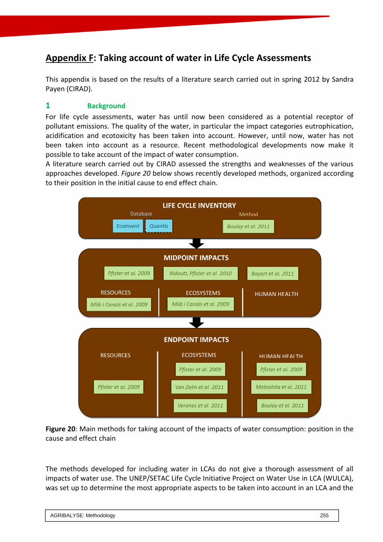
AGRIBALYSE: Methodology 255
Appendix F: Taking account of water in Life Cycle Assessments
This appendix is based on the results of a literature search carried out in spring 2012 by Sandra Payen (CIRAD).
1 Background
For life cycle assessments, water has until now been considered as a potential receptor of pollutant emissions. The quality of the water, in particular the impact categories eutrophication, acidification and ecotoxicity has been taken into account. However, until now, water has not been taken into account as a resource. Recent methodological developments now make it possible to take account of the impact of water consumption. A literature search carried out by CIRAD assessed the strengths and weaknesses of the various approaches developed. Figure 20 below shows recently developed methods, organized according to their position in the initial cause to end effect chain.
Figure 20: Main methods for taking account of the impacts of water consumption: position in the cause and effect chain
The methods developed for including water in LCAs do not give a thorough assessment of all impacts of water use. The UNEP/SETAC Life Cycle Initiative Project on Water Use in LCA (WULCA), was set up to determine the most appropriate aspects to be taken into account in an LCA and the
LIFE CYCLE INVENTORY Database Method
MIDPOINT IMPACTS
ENDPOINT IMPACTS
ECOSYSTEMS HUMAN HEALTH
HUMAN HEALTH ECOSYSTEMS

AGRIBALYSE: Methodology 256
impacts of water use. Bayart et al (2010) defined the complete theoretical framework for taking account of water in an LCA which should serve as a basis for future methodological developments. For characterization factors, however, they refer to the existing methods cited above and the method developed by Pfister et al 2009.
2 Method selected
Although it is disputed, the framework proposed by Pfister et al (2009) was the most advanced and was in a usable state. It was the only method which analyzed the mid and end point impacts for ecosystems, human health and resources using regionalized characterization factors taking account of the local scarcity of water in drainage basins, with global coverage. The local characterization factors, calculated with a spatial resolution of 5 minutes of arc, are available free on line on a GIS layer compatible with Google Earth. Data required for implementing this method The data required to implement this method are the quantity of fresh water consumed (not drawn off) by the production processes and the location of these take off points. A distinction can be drawn between the water consumed directly by farms (water for irrigation, cleaning, drinking, etc) and the water consumed indirectly by the processes related to the product life cycle (water for fabricating inputs).
Direct water use Crop irrigation water (including forage for the animals), cleaning water, drinking water for the animals. Ideally, the LCI data set should be based on primary data from farms. However, the theoretical water requirements can be evaluated using the CROPWAT software developed by the FAO, from which rainfall is deducted to give the irrigation water requirements. The effective rainfall can be calculated using the USDA or FAO formulae.
Indirect water use (background) Water consumed for fabricating inputs and for transport. The ecoinvent database gives the quantity of water that may be used during the life cycle of over 4,000 products and processes (although only the quantity of water drawn off is given). Application for AGRIBALYSE The LCI data set produced for AGRIBALYSE is currently unable to use the method developed by Pfister as the quantity of water drawn off was entered into the data collection module. It is necessary to calculate the water consumed and to locate the place where the water was drawn off before this method can be used. The Pfister method only takes account of water consumed. In agriculture, some of the water may drain back into the aquifer by drainage and/or excessive irrigation. The AGRIBALYSE LCI data set will, therefore, quantify the volume of water drawn off. Calculating the impact of water use using the method proposed by Pfister is one of the priorities for future development of the program. Bibliography Bayart J.B. and Aoustin E., 2011. The Water Impact Index, a simplified single indicator for water
footprinting. LCM 2011 - Towards Life Cycle Sustainability Management, Berlin, Conference presentation.

AGRIBALYSE: Methodology 257
Bayart J.B., Bulle C., Koehler A., Margni M., Pfister S., Vince F. and Deschenes L., 2010. A framework for assessing off stream freshwater use in LCA. International Journal of Life Cycle Assessment, 15 (5): 439-453.
Berger M. and Finkbeiner M., 2010. Water Footprinting: How to Address Water Use in Life Cycle Assessment?. Sustainability, 2 (4), 919-944.
Boulay A.M., Bouchard C., Bulle C., Deschenes L. and Margni M., (2011). Categorizing water for LCA inventory. International Journal of Life Cycle Assessment, 16 (7): 639-651.
Cooney C., 2009. LCA finally takes water into account. Environmental Science and Technology, 43 (11): 3986-3986.
Hoekstra A.Y., Chapagain A.K., Aldaya M.M. and Mekonnen M.M., 2011. The Water Footprint Assessment Manual; Setting the Global Standard. www.waterfootprint.org
Jeswani H K. and Azapagic A., 2011. Water Footprint: Methodologies And a Case Study for Assessing the Impacts of Water use. Journal of Cleaner Production (accepted manuscript)
Milà i Canals L., Chenoweth J., Chapagain A., Orr S., Antón A. and Clift R., 2009. Assessing freshwater use impacts in LCA: Part I - Inventory modeling and characterisation factors for the main impact pathways. International Journal of Life Cycle Assessment, 14 (1), 28-42.
Motoshita M., Itsubo N. and Inaba A., 2011. Development of impact factors on damage to health by infectious diseases caused by domestic water scarcity. International Journal of Life Cycle Assessment, 16 (1): 65-73.
Pfister S., Koehler A. and Hellweg S., 2009. Assessing the environmental impacts of freshwater consumption in LCA. Environmental Science & Technology, 43 (11), 4098-4104
Raimbault M. and Humbert, S. ISO considers potential standard on water footprint. http://www.iso.org/iso/iso-focus-plus_index/iso-focusplus_online-bonus-articles/isofocusplus_bonus_water-footprint.htm
Ridoutt B.G. and Pfister S., 2010. A revised approach to water footprinting to make transparent the impacts of consumption and production on global freshwater scarcity. Global Environmental Change, 20, 113-120.
Roux P., 2011. Le statut de l’eau dans les ACV. Présentation lors de la formation ACV à Montpellier SupAgro.
van Zelm R., Schipper A.M., Rombouts M., Snepvangers J. and Huijbregts M.A.J., 2011. Implementing Groundwater Extraction in Life Cycle Impact Assessment: Characterization Factors Based on Plant Species Richness for the Netherlands. Environmental Science & Technology, 45 (2): 629-635.
Verones F., Hanafiah M.M., Pfister S., Huijbregts M.A.J., Pelletier G.J. and Koehler A. , 2010. Characterization Factors for Thermal Pollution in Freshwater Aquatic Environments. Environmental Science & Technology, 44 (24): 9364-9369.

AG
RIB
ALY
SE
: Me
thodolo
gy
258
Appendix G: Assignment of data collection module inputs to ecoinvent LCI data sets Describing agricultural system requires to describe and quantify all the inputs inf the farming systems. The correspondance between Input names and background LCI is managed through Means-InOut platform (INRA 2016). Bibliography INRA 2015 MEANS (MulticritEria AssessmeNt of Sustainability) Platform https://www6.inra.fr/means/Presentation

AG
RIB
ALY
SE
: Me
thodolo
gy
259
Appendix H: Composition of organic fertilizers The DM content of organic fertilizers was provided b the technical insitutes. When no data was available, we used SALCA references, then as last option we used an average by “fertilizer type”.
Table 151: Composition of organic fertilizers
Organic fertilizer DM (% whole
matter)
OM (% whole
matter)
ASH (% whole
matter)
Total N (kg/t)
N-NH4 (kg/t)
Available N (%)
Plant available N (kg/t)
P2O5 (kg/t)
K2O (kg/t)
MgO (kg/t)
SO3 (kg/t)
Reference
Sewage sludge 7.62 7.23 1.02 Sludge data
Limed sewage sludge 7.5 8 1 6
Composted sewage sludge 7 7 1.5 6
Liquid sewage sludge 3 2.5 0.9 6
Semi-solid sewage sludge 10 7.5 0.8 6
Dried sewage sludge 40 60 5 6
Straw rich cattle compost 33 21 12 8 0.4 5 14 1
Straw rich pig compost 45.3 28.3 17 13.3 1.4 18.4 24.8 7.1 11.1 4
Sheep manure compost 36 26 10 11.5 0.575 7 23 2
Straw rich pig slurry 24.8 14.7 10.1 6.1 1.7 8.8 7.4 6.2 4.1 4
Household waste compost 6 4 5 4 5
Green waste compost 8 4 10 1 10
Sugar scum (alkaline amendment) 3 8.5 0.4 5 10 10
Effluent with low solids 0.35 0.2 9 0.35 0.23 0.135 0.425 1
Feather meal 130 7
Dry poultry droppings 77.5 55.1 22.4 38.2 4.0 90 34.3 37.9 25.3 7.7 11
Average cattle manure 20.6 17.0 3.6 5.5 1.1 2.3 7.9 1
Bedded pack cattle manure 22.1 18 4.1 5.8 0.6 2.3 9.6 1
Wet cattle manure 19 16 3 5.1 1.5 2.3 6.2 1
Duck manure (ready for force feeding) 25 20 5.0 5.43 1.63 90 4.89 7.07 6.29 11
Goat manure 45 36 9 6.1 0.61 5.2 7 2
Turkey manure 57.5 46.6 11.0 18.5 5..2 90 16.7 12.9 13.8 3.9 11
Straw rich pig manure 30.8 23.6 7.2 9.4 3 7.7 14 3.4 5 4
Layer manure 60.0 37.7 22.4 15.0 4.8 90 13.5 21.9 18.2 12
Broiler manure 67.5 56.8 10.8 19.1 3.3 90 17.2 13.9 18.4 4.7 3.7 11
Horse manure 35.1 27.8 22.2 4.84 0.49 3.05 8.46 3
Sheep manure 30 23 7 6.7 0.67 4 12 2

AG
RIB
ALY
SE
: Me
thodolo
gy
260
Organic fertilizer DM (% whole
matter)
OM (% whole
matter)
ASH (% whole
matter)
Total N (kg/t)
N-NH4 (kg/t)
Available N (%)
Plant available N (kg/t)
P2O5 (kg/t)
K2O (kg/t)
MgO (kg/t)
SO3 (kg/t)
Reference
Average cattle slurry 7.5 6.0 6.0 2.6 1.3 1.0 3.1 1
Diluted cattle slurry 5 4 12 1.6 0.8 0.8 2.4 1
Undiluted cattle slurry 10 8 0 3.5 1.75 1.2 3.8 1
Duck manure (for roasting or force fed) 12.5 10 2.5 6.16 2.48 90 4.928 5.4 5.1 1.9 11
Rabbit slurry 28 20.9 7.1 7.6 0.5 80 6.08 11.8 5.9 2 13
Mixed pig slurry 3.6 2.5 1.1 3.5 2.5 2.1 2.5 0.6 0.7 4
Beef calf slurry 1.1 0.5 0 1.5 1.25 0.4 2.4 1
Chicken manure, outdoor run 23 19.5 3.5 13.8 2.3 40 5.52 17.3 22.9
11 & 14
Turkey manure, outdoor run 23 18.8 4.2 8.6 2.4 40 3.4 11.6 12.4
11 & 14
Layer hen manure, outdoor run 23 17 6 7.3 2.3 40 2.9 7.8 6.35
11 & 14
Duck manure, outdoor run 23 18.4 4.6 13.7 4.1 40 5.48 19.1 17
11 & 14
Pig slurry, fattening, outdoor run 6.84 4.59 2.14 5.8 3.7
3.2 4.8 1.2 1.5 4
Sow manure, gestation, outdoor run 2.33 1.17 0.73 2.2 1.7
1.5 1.5 0.3 0.5 4
Sow manure, suckling, outdoor run 3.15 1.69 0.71 2.8 1.7
1.9 2 0.4 0.6 4
Piglet manure, outdoor run 6.73 4.92 2.26 5.2 2.7
3.6 4.5 1.2 1.7 4
Cattle feces, grazing 20 5.4 14.6
15
Vegethumus 20 5 10 25 8
Concentrated sugar beet vinasse 55 21 0 75 2 10 9

AG
RIB
ALY
SE
: Me
thodolo
gy
261
1 Espagnol and Leterme, 2010
2 IE et al, 2001
3 Pouech, 2009
4 Levasseur, 2005
5 ITB, personal communication
6 Arvalis, personal communication
7 Arvalis, personal communication
8 CTIFL, personal communication
9 ITB according to Deleplanque and Cie, Vinasse conforming to NFU 42001/4.6.1. http://www.deleplanque.fr/coproduits-liquides.htm
10 ITB according to AgroSysteme. http://www.agro-systemes.com/engrais-organiques.php
11 ITAVI, 2003
12 ITAVI, 2003/STA environnement itavi
13 2002 - Environmental impact of rabbit breeding and solutions to reduce this impact
14 CORPEN 2006
15 Personal communication Michel Doreau (INRA Clermont Ferrand) - 26/06/2012

AGRIBALYSE: Methodology 262
Appendix I: Building average fertilizer LCI data sets Table 152 and Table 153 summarize the French average N, P and K fertilizer data sets based on mineral fertilizer sales data provided by UNIFA for the period 2005 to 2009. The data sets were built in two steps. The means for each type of fertilizer used during the period studied were calculated and were assigned to the corresponding ecoinvent fertilizer LCI data sets (Table 152). A breakdown of the fertilizers (Table 153) was used to create average fertilizer LCI data sets for the N, P2O5 and K2O equivalent contents. Step 1: Table 152 gives the annual mean consumption in France for fertilizer for the period 2005 to 2009. Column 2 gives the ecoinvent LCI data set corresponding to each type of fertilizer, defined on the basis of several criteria: a) Direct correspondence: There was an ecoinvent data set for the type of fertilizer. For
example, “Ammonitrates” are assigned to “ammonium nitrate, as N, at regional storehouse, RER” (Table 153).
b) Indirect correspondence: There was no direct ecoinvent LCI data set for the type of fertilizer. However, the information on the composition of the fertilizer (source GESTIM) makes it possible to define the fertilizer as a combination of several existing ecoinvent data sets. For example, “UAN” is produced by combining “Urea, as N, at regional storehouse” and “ammonium nitrate, as N, at regional storehouse, RER”. 1 kg of UAN can be considered as the combination of 0.348 kg urea and 0.457 kg ammonium nitrate (the rest being water, cf “Fraction” column in Table 153).
c) Correspondence with other types of fertilizer: This approach was only used for organo mineral fertilizers. N, P2O5 and K2O nutrients from these fertilizers were added pro rata to all the other forms of fertilizer used (Table 153).
Step 2: Table 153 lists the quantities of ingredients of the fertilizers applied. Column 1 gives the name of the ingredient, column 2 gives the corresponding ecoinvent LCI data set. Columns 3 and 4 give the quantities of the ingredient and nutrient (the same as the corresponding columns in Table 152). Column 5 adds the nutrients from organo-mineral fertilizer amendments. Column 6 gives the fractions of the nutrients that are assigned to different ecoinvent data sets (cf indirect correspondence). Columns 7 and 8 give the final assignment of nutrients to each ecoinvent data set. This data was used to build the average fertilizer LCI data set. For fertilizers, Ecoinvent v3 “transformation processes” have been used, and transport added, following GESTIM references. To assess transportation impacts, it is necessary to know both the distance and the weight of the fertilizers. When the weight was not directly available, because only fertilizing values were provided, then converson factors were applied : Total weight = N x 1/28% + P2O5 x 1/18%+ K2O x 1/25%. Table 155 and Table 156 summarize the calculations for fertilizer transport distances for the fertilizers used in France. The first part (in green) gives information on the source of the

AGRIBALYSE: Methodology 263
fertilizer, means of transport used and distances travelled. The sub-table on the left in blue gives the distances for each type of fertilizer for each “transport model”.

AGRIBALYSE: Methodology 264
Table 152: Mean annual deliveries of fertilizer in France between 2005 and 2009 (Source: UNIFA). Column 3 gives the quantity of fertilizer used, columns 4 to 6 give the quantities of nutrients in this fertilizer. Note: Between 2005 and 2009, each year
1,551,887 t of DAP/MAP were spread on fields which is equivalent to an amendment of 276,495 tonnes of nitrogen (kg N) and 716,727 tonnes of phosphorus (kg P2O5)
Fertilizer Correspondence Tonnage t N t P t K
- AMMONITRATES direct correspondence with existing ecoinvent LCI data set 15,686,424 4,844,129
- UAN indirect correspondence with ecoinvent LCI data sets (GESTIM) 10,301,899 3,055,924
- UREA direct correspondence with ecoinvent LCI data set 3,002,222 1,380,913
- OTHER SIMPLE N direct correspondence with ecoinvent LCI data set 1,437,386 445,655
Total Total 30,427,931 9,726,621
- TSP direct correspondence with ecoinvent LCI data set 922,301
419,621
- OTHER SUPERPHOSPHATES direct correspondence with ecoinvent LCI data set 310,560
60,018
- OTHER SIMPLE P indirect correspondence with ecoinvent LCI data sets (GESTIM) 340,735
61,602
- SIMPLE P - SIMPLE P 1,573,596
541,241
- POTASSIUM CHLORIDE direct correspondence with ecoinvent LCI data set 2,291,553
1 374 932
- OTHER SIMPLE K direct correspondence with ecoinvent LCI data set 494,259
196 211
- SIMPLE K - SIMPLE K 2,785,812
1 571 143
- SUPERPOTASSIUM indirect correspondence with ecoinvent LCI data sets (GESTIM) 2,705,710
498,433 658 114
- PHOSPHORUS POTASSIUM indirect correspondence with ecoinvent LCI data sets (GESTIM) 377,562
51,184 65 095
- OTHER PK indirect correspondence with ecoinvent LCI data sets (GESTIM) 773,807
87,895 132 845
- BINARY PK - BINARY PK 3,857,079
637,512 856 054
- DAP - MAP direct correspondence with ecoinvent LCI data set 1,551,877 276,495 716,727
- OTHER NP direct correspondence with ecoinvent LCI data set 1,005,782 204,965 171,532
- NK - NPK indirect correspondence with ecoinvent LCI data sets (GESTIM) 6,717,677 996,357 677,445 1 075 104
- ORGANO-MINERAL added to N P K of the LCI data sets pro rata to N / P / K composition
605,745 27,057 35,913 59 098
- NP, NK, NPK, ORGANO-MINERAL COMPOUNDS
- NP, NK, NPK, ORGANO-MINERAL COMPOUNDS 9,881,081 1,504,874 1,601,617 1 134 202

AGRIBALYSE: Methodology 265
Table 153: AGRIBALYSE average fertilizer LCI data sets according to N/P/K composition Note (row UAN): Between 2005 and 2009, in France, each year 10,301,899 t of UAN were applied which is equivalent to an amendment of 3,055,924 tonnes of nitrogen (kg N). For the average fertilizer, the fraction from organo mineral fertilizers for this nutrient (27,057 t N) was allocated pro rata to all the LCI data sets. This corresponds to an additional 7,379 t N for UAN (column t N + pro rata). As ecoinvent does not have a UAN data set, UAN was split using GESTIM data making each kg UAN equivalent to 0.348 kg urea and 0.457 kg ammonium nitrate (cf “Fraction” column). The UAN applied can be considered to be 1,324,260 t N in the form of urea and 1,739,043 t of N in the form of ammonium nitrate. The last column gives the contribution of UAN to 1 kg of all N amendment in France: 118 g (included in the average fertilizer LCI data set as “urea”) and 155 g (included in the average fertilizer LCI data set as “ammonium nitrate”).
Average mineral fertilizer, as N, at regional storehouse, FR
Ingredient ecoinvent LCI data set t t N t N + pro rata Fraction t N LCI data
set
- AMMONITRATES Ammonium nitrate, as N {RER}| ammonium nitrate production | Alloc Rec 15,686,424.00 4,844,129.00 4,855,826.83 1 4,855,826.83 0.432
- UAN Urea, as N {RER}| production | Alloc Rec 10,301,899.00 3,055,924.00 3,063,303.59 0.348 1,324,260.43 0.118
Ammonium nitrate, as N {RER}| ammonium nitrate production | Alloc Rec
0.457 1,739,043.15 0.155
- UREA Urea, as N {RER}| production | Alloc Rec 3,002,222.00 1,380,913.00 1,384,247.69 1 1,384,247.69 0.123
- OTHER N FERTILIZER Ammonium sulfate, as N {RER}| ammonium sulfate production | Alloc Rec 1,437,386.00 445,655.00 446,731.19 1 446,731.19 0.040
- DAP - MAP Nitrogen fertiliser, as N {RER}| diammonium phosphate production | Alloc Rec 1,551,877.00 276,495.00 277,162.69 1 277,162.69 0.025
- OTHER NP FERTILIZER Phosphate fertiliser, as P2O5 {RER}| ammonium nitrate phosphate production | Alloc Rec 1,005,782.00 204,965.00 205,459.96 1 205,459.96 0.018
- NK - NPK Ammonium nitrate, as N {RER}| ammonium nitrate production | Alloc Rec 6,717,677.00 996,357.00 998,763.05 0.45 449,443.37 0.040
Urea, as N {RER}| production | Alloc Rec
0.25 249,690.76 0.022
Ammonium sulfate, as N {RER}| ammonium sulfate production | Alloc Rec
0.2 199,752.61 0.018
Nitrogen fertiliser, as N {RER}| monoammonium phosphate production | Alloc Rec
0.1 99,876.30 0.009
- ORGANO-MINERAL repartis sur les autres 605,745.00 27,057.00
TotaL 40,309,012.00 11,231,495.00 11,231,495.00
11,231,495.00 1.000
average mineral fertilizer, as P2O5, at regional storehouse, FR
Ingredient ecoinvent LCI data set t t P t P allocated Splitting t P LCI data set
- TSP Phosphate fertiliser, as P2O5 {RER}| triple superphosphate production | Alloc Rec 922,301.00 419,621.00 425,112.01 1 425,112.01 0.153
- OTHER SUPERPHOSPHATES Phosphate fertiliser, as P2O5 {RER}| single superphosphate production | Alloc Rec 310,560.00 60,018.00 60,803.37 1 60,803.37 0.022
- OTHER P FERTILIZER Phosphate fertiliser, as P2O5 {RER}| single superphosphate production | Alloc Rec 340,735.00 61,602.00 62,408.10 1 62,408.10 0.022

AGRIBALYSE: Methodology 266
- DAP - MAP Phosphate fertiliser, as P2O5 {RER}| diammonium phosphate production | Alloc Rec 1,551,87.,00 716,727.00 726,105.84 1 726,105.84 0.261
- OTHER NP FERTILIZER Phosphate fertiliser, as P2O5 {RER}| ammonium nitrate phosphate production | Alloc Rec 1,005,782.00 171,532.00 173,776.61 1 173,776.61 0.063
- NK - NPK Nitrogen fertiliser, as N {RER}| monoammonium phosphate production | Alloc Rec 6,717,677.00 677,445.00 686,309.81 0.6 411,785.88 0.148
Phosphate fertiliser, as P2O5 {RER}| ammonium nitrate phosphate production | Alloc Rec
0,3 205 892,94 0,074
Phosphate fertiliser, as P2O5 {RER}| triple superphosphate production | Alloc Rec
0.1 68,630.98 0.025
- ORGANO-MINERAL repartis sur les autres 605,745.00 35,913.00
0.000
- SUPERPOTASSIUM Phosphate fertiliser, as P2O5 {RER}| triple superphosphate production | Alloc Rec 2,705,710.00 498,433.00 504,955,32 1 504,955.32 0.182
- PHOSPHORUS POTASSIUM Phosphate fertiliser, as P2O5 {RER}| triple superphosphate production | Alloc Rec 377,562.00 51,184.00 51,853,78 1 51,853.78 0.019
- OTHER PK Phosphate fertiliser, as P2O5 {RER}| triple superphosphate production | Alloc Rec 773,807.00 87,895.00 89,045,16 1 89,045.16 0.032
Total 15,311,756.00 2,780,370.00 2,780,370.00
2,780,370.00 1.000
Average mineral fertilizer, as K2O, at regional storehouse, FR
Ingredient ecoinvent LCI data set t t K t K allocated Splitting t P LCI data set
- POTASSIUM CHLORIDE Potassium sulfate, as K2O {RER}| potassium sulfate production | Alloc Rec 2,291,553.00 1,374,932.00 1,398,132.67 1 1,398,132.67 0.393
- OTHER K FERTILIZER Potassium sulfate, as K2O {RER}| potassium sulfate production | Alloc Rec 494,259.00 196,211.00 199,521.87 1 199,521.87 0.056
- SUPERPOTASSIUM Potassium chloride, as K2O {RER}| potassium chloride production | Alloc Rec 2,705,710.00 658,114.00 669,219.05 1 669,219.05 0.188
- PHOSPHORUS POTASSIUM Potassium chloride, as K2O {RER}| potassium chloride production | Alloc Rec 377,562.00 65,095.00 66,193.42 1 66,193.42 0.019
- OTHER PK Potassium chloride, as K2O {RER}| potassium chloride production | Alloc Rec 773,807.00 132,845.00 135,086.63 1 135,086.63 0.038
- NK - NPK Potassium chloride, as K2O {RER}| potassium chloride production | Alloc Rec 6,717,677.00 1,075,104.00 1,093,245.36 0,8 874,596.29 0.246
Potassium sulfate, as K2O {RER}| potassium sulfate production | Alloc Rec
0,2 218,649.07 0.061
- ORGANO-MINERAL repartis sur les autres 605,745.00 59,098.00
0.000
Total 13,966,313.00 3,561,399.00 3,561,399.00
3,561,399.00 1.000

AGRIBALYSE: Methodology 267
Table 154: Example of 8-10-20 mineral fertilizer
Composition of 8-10-20 fertilizer Correspondence
Content kg/t Factor LCI data set
N average mineral fertilizer, as N, at regional storehouse, FR
80 1.00 80.00
P average mineral fertilizer, as P2O5, at regional storehouse, FR
100 1.00 100.00
K average mineral fertilizer, as K2O, at regional storehouse, FR
200 1.00 200.00
other components Production of other components is ignored, but the quantity is taken into account for transport 620
Total 1000
Table 155: Recalculation of transport models for fertilizers, based on GESTIM (GAC et al, 2010)
Distance (km) Source
Means of transport F EU 15 Russia Ukraine N Africa Arabia Cent America Chile Qatar China /Austr
Road 150 400 150 150 150 150 150 150 150 150
Boat
1500 5000 2500 3500 4000 6500 6000 1000
Type of fertilizer
Ammonia 100%
Urea 0% 30% 26% 0% 35% 0% 8% 0% 0% 1%
AN / CAN 52% 40% 8% 0% 0% 0% 0% 0% 0% 0%
UAN 55% 16% 25% 2% 2% 0% 0% 0% 0% 0%
MAP/DAP 0% 16% 8% 8% 67% 0% 0% 0% 1% 0%
TSP 10% 26% 0% 0% 61% 0% 0% 0% 3% 0%
Potassium 0% 97% 2% 0% 0% 0% 0% 0% 1% 0% Transport model (tkm) GESTIM Original
Type Road Boat
Transport Lorry > 16,t aver. RER
transport, transoceanic freight ship ; OCE
TM N fertilizer 150 0
TM Urea 225 1595
TM AN/CAN 250 120
TM UAN 190 525
TM MAP/DAP 190 2255
TM TSP 215 1705
TM Potassium 392.5 90
TM Average fertilizer 230.36 898.57
Table 156: Assignment of Transport models (TM) to LCI data sets

AGRIBALYSE: Methodology 268
Fertilizer LCI data sets used for AGRIBALYSE
Tr Model
average mineral fertilizer, as K, at regional storehouse, FR TM Potassium
average mineral fertilizer, as N, at regional storehouse, FR TM N fertilizer
average mineral fertilizer, as P, at regional storehouse, FR TM TSP
ICV ecoinvent Copper, primary, at refinery/RER U TM Average
ICV ecoinvent ammonium nitrate, as N, at regional storehouse, RER TM AN/CAN
ICV ecoinvent calcium nitrate, as N, at regional storehouse, RER TM AN/CAN
ICV ecoinvent chemicals inorganic, at plant, GLO TM Average
ICV ecoinvent diammonium phosphate, as N, at regional storehouse, RER TM MAP/DAP
ICV ecoinvent Magnesium oxide, at plant, RER TM Average
ICV ecoinvent Zinc, primary, at regional storage/RER U TM Average
ICV ecoinvent Manganese oxide (Mn2O3), at plant, CN TM Average
ICV ecoinvent Lime, from carbonation, at regional storehouse, CH TM Average
ICV ecoinvent Limestone, milled, loose, at plant, CH TM Average
ICV ecoinvent Magnesium sulphate, at plant, RER TM MAP/DAP
ICV ecoinvent Monoammonium phosphate, as N, at regional storehouse TM MAP/DAP
ICV ecoinvent Potassium chloride, as K2O, at regional storehouse. RER TM Potassium
ICV ecoinvent Potassium nitrate, as K2O, at regional storehouse, RER TM Potassium
ICV ecoinvent Potassium sulphate, as K2O, at regional storehouse, RER TM Potassium
ICV ecoinvent Single superphosphate, as P2O5, at regional storehouse, RER TM TSP
ICV ecoinvent Triple superphosphate, as P2O5, at regional storehouse, RER TM TSP
ICV ecoinvent Urea ammonium nitrate, as N, at regional storehouse, RER TM Urea
ICV ecoinvent Urea, as N, at regional storehouse TM Urea
ICV ecoinvent Ammonium sulphate, as N, at regional storehouse, RER TM N fertilizer

AGRIBALYSE: Methodology 269
Appendix J: Building the machinery data sets Table 157 gives the groups of machinery used for the data collection module and the data required for parameterizing the ecoinvent LCI data set (see B.2.1). Of the 191 machines defined in AGRIBALYSE® data collection module, 186 can be assigned to one of the six existing “agricultural machinery” LCI data sets in ecoinvent v2.0: - tractors; harvesters; trailers; agricultural machinery, general; agricultural machinery, tillage; slurry tankers. A new LCI data set “electric machinery” has been created for the remaining 5 AGRIBALYSE® machines. These 7 groups (6+1) were subdivided according to the life times of machines to take into account the different use of a certain number of components (tires, oil and filters for the engine). This gives a total of 14 machinery groups with an average lifetime and weight (see row in blue gray). These groups (1st column) correspond to the 14 AGRIBALYSE® machinery LCI data sets, based on ecoinvent and parametrized according to weight and lifetime of machines in use in France. The unit processes for these 14 groups of machine are given in Table 157. Table 157: Groups of machines listed in the data collection module as 14 AGRIBALYSE groups of machines
Groups of machines and summary of values used
for the "production machine XY" data set Machine in the DCM Rating (kW); width (m), capacity (m
3) Life time (h)
Weight of
machine (kg)
Tractor, LT 7'500h, production (based on Tractor) Tracked vehicle 7200 450
Vineyard tractor 7200 2300
Tractor 30 kW 28 kW 7200 1375
Tractor 50-60 kW 50-60 kW 7200 3'000
Tractor, soil disinfection contractor 257 kW (350 bhp), 4 WD 7500 11800
Value used 7200 5400
Tractor, LT 10'000h, production (based on Tractor)
Mini tractor Kubota L3608 20 kW 9000 1100
Telescopic 100 bhp 10000 4500
Tractor 200 bhp 147 kW (200 bhp), 4 WD 9600 9000
Tractor 80-100 kW (110-140 bhp) 110-140 bhp (80-100 kW) 10000 5300
Tractor 80-100 KW (110-140 bhp) 10000 5300
Orchard tractor 51.4 kW, 4 WD 51.4 kW 10500 2400
Value used for 10000 4500
Tractor, LT 12’000h, production (based on Tractor) High clearance tractor 44.1 kW 4 WD 44.1 12000 2200
High clearance tractor 73.5 kW, 4 WD 73.5 12000 4000
High clearance cultivator gasoline 15000 800

AGRIBALYSE: Methodology 270
Groups of machines and summary of values used
for the "production machine XY" data set Machine in the DCM Rating (kW); width (m), capacity (m
3) Life time (h)
Weight of
machine (kg)
Self driver 265 kW 12000 5500
Self propelled 360 kW 12000 5500
Tractor 160 bhp, 4 WD 160 bhp 12000 6440
Tractor 300 bhp 300 bhp 12000 9500
Tractor 58.8 kW 4 WD 58.8 12000 2800
Tractor 77.2 kW, 4 WD 77.2 kW 12000 3500
Tractor 90 bhp, 4 WD 90 bhp 12000 4300
Tractor Massey Ferguson 50 kW 15000 2358
Tractor TMF 275 (Mango) 77.2 15000 3000
Back hoe loader 104 kW 12000 20600
Value used 12000 5500
Harvester/Machine with engine, LT < 5'000h, production (based on Harvester) Self-propelled vine lifter 3000 5000
Self-propelled sugar beet harvester 6 rows 265 kW, 6 rows 2500 15100
Self-propelled carrot sprayer Aquitaine 102.9 kW (140 bhp), 3000 l tank, 24 m bar 3600 7335
Self-propelled forage harvester 600 bhp with trailer 600 bhp 4000 9000
Self-propelled forage harvester 8 rows, 480 bhp 4000 9000
Self-propelled grape harvester 3000 5800
Combine harvester, 200 bhp, 5.5m 200 kW, 5.5 m 4000 10000
Cultivator with water pump 1600l/min 4kW 700 30
Quad 5 bhp 1600 285
Value used 3000 8000
Harvester/Machine with engine, LT 5'000-10’000h, production (based on Harvester)
Self-propelled harvester 3 rows 147 kW (200 bhp) 6000 14000
Sprayer 18 bhp engine 13 kW 7200 150
Self-propelled harvester 6400 9500
Self-propelled carrot harvester 147 kW (200 bhp) 6000 14000
Value used 7200 5400
Harvester/Machine with engine, LT > 10'000h, production (based on Harvester)
Self-propelled sprayer 220 kW (300 bhp) 18000 9100
Self-propelled work platform 14.7 kW 12000 2250
Value used 15000 6000
Trailer, < 20 t, production (based on Trailer) Trailer (Clementine harvester) na 10000 500
Trailer 4 palox crates 6000 760

AGRIBALYSE: Methodology 271
Groups of machines and summary of values used
for the "production machine XY" data set Machine in the DCM Rating (kW); width (m), capacity (m
3) Life time (h)
Weight of
machine (kg)
Trailer, 12-14t 12-14 t, 2 axles 6000 5139
Trailer, 16-18t 16-18 t, 2 axles 6000 6590
Trailer, 8t 8 t, 2 axles 6000 4'084
Value used 6000 3500
Trailer, > 20 t, production (based on Trailer) Trailer body 21 tonnes 21 tonnes 15000 8100
Trailer body, 2 axles - 15 t 6000 5883
Value used 10000 7000
Slurry tanker 5’000 lt, production (based on Slurry tanker) Slurry spreader / 5000l vacuum tank 5000 l 5000 1690
Value used 5000 1700
General machinery, with tires, LT < 2'500h, production (based on Agricultural machinery, general)
Potato harvester 2 rows, standard, 75 cm 1800 5500
Baler 17 bales / h 17 bales / h 1000 2000
Manure spreader, 5t 5t 2400 3848
Fertilizer spreader, centrifugal, 1500l 24 m, 1500 l 800 550
Planter, 4 rows, 75 cm 4 rows 1500 2000
Maiden tree planter 1000 500
Nursery planter, 4 rows 4 rows 2250 1060
Nursery planter/transplanter 2250 300
Duster for orchards Towed 600 liters 240 260
Round baler
1800 1773
Cider apple harvester 1875 1200
Rice combine harvester Kaset Phattana 120 kW, 3 m 2000 4000
Disk drill for no till, 4m 4 m 1200 5300
Standard drill, 4m 4 m 1200 1000
Tine coulter drill 3 m 900 680
Tine coulter drill(3 m) 3 m 900 680
Single seed drill, pneumatic delivery - 6 rows 6 rows (3m) 1200 1000
Value used 1500 2000
General machinery, with tires, LT 2'500-5’000h, production (based on Agricultural machinery, general)
Swather 9m 9 m 3000 3200
Towed carrot harvester 1 row 1 row 4800 5500
Towed sprayer, 2000 L, two horizontal turbines 2000 L 4000 650
Slurry spreader with hanging bar, 1500-2000l 1 axle, 1500-2000 l 5000 1000

AGRIBALYSE: Methodology 272
Groups of machines and summary of values used
for the "production machine XY" data set Machine in the DCM Rating (kW); width (m), capacity (m
3) Life time (h)
Weight of
machine (kg)
Manure spreader, 8-10t 2 axles, 8-10 t 5000 3500
Soil disinfection machine 13 coulters, 4,75 m, 2 1000 l tanks 4500 3500
Potato planter, 4 rows, 75 cm 4 rows 75 cm automatic 3000 1000
Spreader Jacto Arbus 2000 (Mango) 2000 820
Towed sprayer, 2500l 24 m, 2500 l 3000 2600
3 strip seed drill 5.5 m 3600 2250
Pneumatic seed drill 900 550
Value used 4000 2500
General machinery, with tires, LT > 5'000h, production (based on Agricultural machinery, general)
Towed swather1.83 m 1.83 m 6000 3370
Towed carrot harvester 3 rows 3 rows 6000 9000
3 strip spreader, 6-8 tonnes 6-8 tonnes 9000 3120
Towed sprayer, 3000l 24 / 28 m, 3000 l 6000 2500
Towed carrot harvester 6000 9000
Value used 7800 6200
machine portée (basée sur "Agricultural machinery, tillage"
Swather for pruning wood 2.5 m 200 250
Nursery maiden tree lifter 7200 1500
Sprayer 2300 900
Hoeing machine 2300 900
Hoeing machine, 2 rows 2.5 m 2400 450
Hoeing machine, 3.6 m 1800 550
Hoeing machine, with camera, 4 m camera, 4 m, tines 3000 1600
Three row hoeing machine 5.5 m 4800 770
Hoeing machine for grapevines 2.5 1500 550
Flail shredder 4.5 2300 2100
Flail 2.5 m 200 645
Pruning shredder (vines) 2300 530
Pruning shredder (clementines) na 1000 500
Haulm topper 4 rows 3000 1000
Haulm topper (carrots) 4.8 m 2400 2600
Ridger 4 rows 3000 1000
Ridger with roller molders 2 ridges 2400 300
Ridger for tunnel 450 450

AGRIBALYSE: Methodology 273
Groups of machines and summary of values used
for the "production machine XY" data set Machine in the DCM Rating (kW); width (m), capacity (m
3) Life time (h)
Weight of
machine (kg)
Plow, single, reversible 3000 1350
Plow, single 3000 400
Plow, 5 furrow, 3 point 5 furrow, 3 point 3000 1000
Plow, 8 furrow 3.2 m 4800 3150
Disk plow, Kubota 3-4 disks 1500 200
Plow, 4 furrow, attachment 4 furrow 480 1039
Furrow plow 2500 163
Plow for grapevines, single 900 150
Plow, 6 furrow 4800 1760
Chisel plow, 2.5m 2.5 m 2300 709
Chisel plow, 4.5m 4.5 m 1570 1029
Compressor attachment 2300 900
Compressor attachment for secateurs compressor + 600 l tank 3750 500
Disk harrow (Mangoes) 2500 1000
Harrow. 36 disk. 5.5m 2300 3000
Disk harrow, 4m 4 m 2100 3000
Heavy cultivator + roller 3 m 2400 1300
Rotary tiller, 2m 2 m 2300 330
Triple bed former 5.5 m 3600 3900
Under vine weeder 2300 800
Disk harrow 2.5 m 2.5 m 800 780
Disk harrow, independent disks, 4m 4 m 1500 2100
Disk harrow, semi attached, 5.5 m 5.5 m 3600 3900
Disk harrow attachment, 5.5m 5.5 1500 2100
Chisel plow, 4 m 4 m 4800 1000
Chisel plow, 7 chisels 7 chisels 2400 1000
Chisel plow, 5 chisels 3 3000 900
Chisel plow 2300 1000
Wire unspooler 2250 80
Hail net unspooler 2250 600
Weed burner 1500 550
Disk for harrow 300 200

AGRIBALYSE: Methodology 274
Groups of machines and summary of values used
for the "production machine XY" data set Machine in the DCM Rating (kW); width (m), capacity (m
3) Life time (h)
Weight of
machine (kg)
Topping machine 1800 200
Leaf stripper 1800 500
Leaf stripper (vines) 2300 100
3 point forklift 6000 460
Post driver 3000 335
Post driver 2300 700
Stone burier 2.1 m 1500 860
Spooler 2250 400
Forage harvester attachment, single row 1 row 3000 480
Chemical vine disbudder 2300 450
Mechanical vine disbudder 2300 450
Spreader 500 l 1800 126
Fertilizer spreader 500 l 1.45 m 800 126
Spreader attachment. 1000 kg 1000 kg 2300 150
Spreader attachment, 2500 l 28 800 463
Fertilizer spreader, centrifugal, 500 l 500 l 2300 193
Tedder, 3 m 3000 370
Mower, 7 m 7 m 1500 3200
Mower conditioner attachment, 3m 3 m 1500 1075
Rotary mower, 3m 3 m 2300 643
Binder 1800 150
Front forklift 1000 150
Rotary cultivator, 4 m 4 m 1800 1270
Front bucket 2.1 m 900 320
Tine harrow 2300 600
Rotary topper 2300 900
Rotary topper. orchard 3.6 m 700 530
Gyro-cep rotary topper sunflower 2300 200
Reciprocating harrow. 3m 3m 2300 1686
Vibrating harrow with roller 2.05 m 900 625
Chain harrow for mechanical weeding, 12m 610 1020
Rotary harrow 4 m 1800 1380

AGRIBALYSE: Methodology 275
Groups of machines and summary of values used
for the "production machine XY" data set Machine in the DCM Rating (kW); width (m), capacity (m
3) Life time (h)
Weight of
machine (kg)
Rotary harrow+ roller 2 m 750 780
Rotary harrow with roller 3 m 1800 960
Rotary harrow, 4m 4 m 2010 1686
Rotary harrow, with roller 2,5 m 2.5 m 800 840
Rotary harrow 300 500
Injector for soil disinfection 1800 300
Intervine blade 1500 40
Cutter for trimming fruit tree row 500 750
Soil disinfection machine, Normandy 10 coulters 2400 800
Scarifier, 5.5 5.5 m 2300 552
Triple mulching film laying machine 3 strips 1.65 to 1.90 m 2400 1000
Bale trailer 6000 3150
Coarse pruner 2300 900
Sprayer 2000 l with cannon 4000 800
Sprayer 3400 l, 24 m 24 m 3000 2300
Backpack sprayer Mitsubishi TU 26 2 kW 2300 12
Recycling tunnel sprayer
2300 450
Lance sprayer na 1000 200
Sprayer, 1200 l tank, 18 m bar 3000 650
Sprayer attachment 1000L, 24 m bar 24 m 4800 990
Sprayer attachment 400 l 2 m 3000 200
Sprayer attachment 600 L, 4 rows 4 rows 3000 500
Sprayer attachment 800 l with 12 m bar 12 m 4800 950
Sprayer attachment , 800l 15 m, 800 l 2300 477
Sprayer greenhouse, vertically trained crops 20 bhp, 400 liter tank, vertical bar 2400 500
Sprayer 18 m, 1200 l 18 m, 1200 l 3000 1000
Spray bar 2300 150
Ditcher 4800 400
Trimming machine 2300 900
Rotavator 2 m 1800 405
Rotavator 4800 685
Rotavator 3 m 3 m 2400 1000

AGRIBALYSE: Methodology 276
Groups of machines and summary of values used
for the "production machine XY" data set Machine in the DCM Rating (kW); width (m), capacity (m
3) Life time (h)
Weight of
machine (kg)
Spader 2 m 1800 830
Tedder 3 1500 300
Roller harrow, 3m 3m, attachment 3000 1130
Roller, 9m 9m 1410 4500
Potato lister 2300 450
Shaker 375 800
Baler stacker 2400 550
Subsoiler, 2 m 375 450
Subsoiler, 6 furrows, 3 m 6 furrows, 3 m 2400 770
Subsoiler 2300 900
Subsoiler 2500 300
Augur 3000 290
Mower, cider apple orchard 3.4 m 3.4 m 700 650
Saw with lance for pruning cider orchards 0.95 kW 500 6.3
Spring tine harrow 6.3 m 1800 910
Spring tine harrow, 3m 3 m 2300 538
Spring tine harrow, 5m 5m, mounted 1300 750
Value used 2300 900
Agricultural machinery with electronic motor, production
Electric fork lift on rails 0.37 kW 2500 300
Conveyor 0,18 kW 1500 41
Brush cutter Honda UMK 435T 2kW, 2m 250 12
Potting machine 4.12 kW 1500 1200
Compost hopper 4 kW 2250 1500
Value used 2300 900

AGRIBALYSE®: Methodology 277
Table 158: Unit processes for the 14 groups of agricultural machinery used in the AGRIBALYSE LCI data sets. The unit processes were calculated by parameterizing the basic ecoinvent LCI data sets with the average life time and average weight (cf table above).
Input Units Quantity Comment
Tractor, LT 10,000h, production/FR. FU = kg per life time, based on “ Tractor, CH” Alkyd paint, white, 60% in solvent, at plant/RER kg 0.005 Production
Aluminium, production mix, at plant/RER kg 0.045 Production
Chromium steel 18/8, at plant/RER kg 0.03 Production
Copper, at regional storage/RER kg 0.02 Production
Electricity, medium voltage, at grid/FR kWh 1.5 Production
Flat glass, uncoated, at plant/RER kg 0.01 Production
Hard coal, burned in industrial furnace 1-10MW/RER MJ 0.84 Production
Lead, at regional storage/RER kg 0.01 Production
Light fuel oil, burned in industrial furnace 1MW, non-modulating/RER MJ 0.84 Production
Lubricating oil, at plant/RER kg 0.0066 Production
Natural gas, burned in industrial furnace >100kW/RER MJ 4.92 Production
Polypropylene, granulate, at plant/RER kg 0.03 Production
Steel, converter, unalloyed, at plant/RER kg 0.67 Production
Steel, low-alloyed, at plant/RER kg 0.07 Production
Synthetic rubber, at plant/RER kg 0.1 Production
Transport, freight, rail/RER tkm 0.1 Production
Transport, lorry >32t, EURO4/RER tkm 0.4 Production
Zinc, primary, at regional storage/RER kg 0.01 Production
Electricity, medium voltage, at grid/FR kWh 0.55939 Maintainance (filter, oil)
Light fuel oil, burned in industrial furnace 1MW, non-modulating/RER MJ 7.1399 Maintainance (filter, oil)
Electricity, medium voltage, at grid/FR kWh 0.4862 Maintainance (tires)
Light fuel oil, burned in industrial furnace 1MW, non-modulating/RER MJ 6.2057 Maintainance (tires)
Lead, at regional storage/RER kg 0.04 Maintenance (filter)
Paper, woodfree, coated, at integrated mill/RER kg 0.008 Maintenance (filter)
Polypropylene, granulate, at plant/RER kg 0.004 Maintenance (filter)
Lubricating oil, at plant/RER kg 0.28453 Maintenance (oil)
Synthetic rubber, at plant/RER kg 0.2925 Maintenance (tires)
Alkyd paint, white, 60% in solvent, at plant/RER kg 0.00125 Repair
Aluminium, production mix, at plant/RER kg 0.01125 Repair
Chromium steel 18/8, at plant/RER kg 0.0075 Repair
Copper, at regional storage/RER kg 0.005 Repair
Electricity, medium voltage, at grid/FR kWh 0.41556 Repair
Flat glass, uncoated, at plant/RER kg 0.0025 Repair
Lead, at regional storage/RER kg 0.0025 Repair
Light fuel oil, burned in industrial furnace 1MW, non-modulating/RER MJ 5.304 Repair
Polypropylene, granulate, at plant/RER kg 0.0075 Repair
Steel, converter, unalloyed, at plant/RER kg 0.1675 Repair
Steel, low-alloyed, at plant/RER kg 0.0175 Repair
Synthetic rubber, at plant/RER kg 0.025 Repair
Zinc, primary, at regional storage/RER kg 0.0025 Repair
Electricity, medium voltage, at grid/FR kWh 0.13889 Waste management
Transport, lorry >32t, EURO4/RER tkm 0.04 Waste management
Carbon dioxide, fossil, low. pop. kg 0.005445 Production
Heat, waste, high. pop. MJ 9.574 Production
NMVOC, non-methane volatile organic compounds, unspecified origin, high. pop. kg 0.0048 Production
NMVOC, non-methane volatile organic compounds, unspecified origin, high. pop. kg 0.0036615 Maintainance (filter, oil)
NMVOC, non-methane volatile organic compounds, unspecified origin, high. pop. kg 0.0031824 Maintainance (tires)
Carbon dioxide, fossil, low. pop. kg 0.0013612 Repair
NMVOC, non-methane volatile organic compounds, unspecified origin, high. pop. kg 0.00272 Repair
Disposal, building, glass sheet, to final disposal/CH kg 0.0025 Waste management
Disposal, building, glass sheet, to final disposal/CH kg 0.01 Waste management
Disposal, paper, 11.2% water, to municipal incineration/CH kg 0.008 Waste management
Disposal, plastics, mixture, 15.3% water, to municipal incineration/CH kg 0.004 Waste management
Disposal, plastics, mixture, 15.3% water, to municipal incineration/CH kg 0.00875 Waste management
Disposal, plastics, mixture, 15.3% water, to municipal incineration/CH kg 0.035 Waste management
Disposal, used mineral oil, 10% water, to hazardous waste incineration/CH kg 0.0066 Waste management
Disposal, used mineral oil, 10% water, to hazardous waste incineration/CH kg 0.28453 Waste management

AGRIBALYSE®: Methodology 278
Input Units Quantity Comment
Tractor, LT 12,000h, production/FR. FU = kg per life time, based on “Tractor, CH” Alkyd paint, white, 60% in solvent, at plant/RER kg 0.005 Production
Aluminium, production mix, at plant/RER kg 0.045 Production
Chromium steel 18/8, at plant/RER kg 0.03 Production
Copper, at regional storage/RER kg 0.02 Production
Electricity, medium voltage, at grid/FR kWh 1.5 Production
Flat glass, uncoated, at plant/RER kg 0.01 Production
Hard coal, burned in industrial furnace 1-10MW/RER MJ 0.84 Production
Lead, at regional storage/RER kg 0.01 Production
Light fuel oil, burned in industrial furnace 1MW, non-modulating/RER MJ 0.84 Production
Lubricating oil, at plant/RER kg 0.0066 Production
Natural gas, burned in industrial furnace >100kW/RER MJ 4.92 Production
Polypropylene, granulate, at plant/RER kg 0.03 Production
Steel, converter, unalloyed, at plant/RER kg 0.67 Production
Steel, low-alloyed, at plant/RER kg 0.07 Production
Synthetic rubber, at plant/RER kg 0.1 Production
Transport, freight, rail/RER tkm 0.1 Production
Transport, lorry >32t, EURO4/RER tkm 0.4 Production
Zinc, primary, at regional storage/RER kg 0.01 Production
Electricity, medium voltage, at grid/FR kWh 0.67127 Maintainance (filter, oil)
Light fuel oil, burned in industrial furnace 1MW, non-modulating/RER MJ 8.5679 Maintainance (filter, oil)
Electricity, medium voltage, at grid/FR kWh 0.61585 Maintainance (tires)
Light fuel oil, burned in industrial furnace 1MW, non-modulating/RER MJ 7.8605 Maintainance (tires)
Lead, at regional storage/RER kg 0.048 Maintenance (filter)
Paper, woodfree, coated, at integrated mill/RER kg 0.0096 Maintenance (filter)
Polypropylene, granulate, at plant/RER kg 0.0048 Maintenance (filter)
Lubricating oil, at plant/RER kg 0.34144 Maintenance (oil)
Synthetic rubber, at plant/RER kg 0.3705 Maintenance (tires)
Alkyd paint, white, 60% in solvent, at plant/RER kg 0.001375 Repair
Aluminium, production mix, at plant/RER kg 0.012375 Repair
Chromium steel 18/8, at plant/RER kg 0.00825 Repair
Copper, at regional storage/RER kg 0.0055 Repair
Electricity, medium voltage, at grid/FR kWh 0.45711 Repair
Flat glass, uncoated, at plant/RER kg 0.00275 Repair
Lead, at regional storage/RER kg 0.00275 Repair
Light fuel oil, burned in industrial furnace 1MW, non-modulating/RER MJ 5.8344 Repair
Polypropylene, granulate, at plant/RER kg 0.00825 Repair
Steel, converter, unalloyed, at plant/RER kg 0.18425 Repair
Steel, low-alloyed, at plant/RER kg 0.01925 Repair
Synthetic rubber, at plant/RER kg 0.0275 Repair
Zinc, primary, at regional storage/RER kg 0.00275 Repair
Electricity, medium voltage, at grid/FR kWh 0.13889 Waste management
Transport, lorry >32t, EURO4/RER tkm 0.04 Waste management
Carbon dioxide, fossil, low. pop. kg 0.005445 Production
Heat, waste, high. pop. MJ 9.574 Production
NMVOC, non-methane volatile organic compounds, unspecified origin, high. pop. kg 0.0048 Production
NMVOC, non-methane volatile organic compounds, unspecified origin, high. pop. kg 0.0043938 Maintainance (filter, oil)
NMVOC, non-methane volatile organic compounds, unspecified origin, high. pop. kg 0.004031 Maintainance (tires)
Carbon dioxide, fossil, low. pop. kg 0.0014974 Repair
NMVOC, non-methane volatile organic compounds, unspecified origin, high. pop. kg 0.002992 Repair
Disposal, building, glass sheet, to final disposal/CH kg 0.00275 Waste management
Disposal, building, glass sheet, to final disposal/CH kg 0.01 Waste management
Disposal, paper, 11.2% water, to municipal incineration/CH kg 0.0096 Waste management
Disposal, plastics, mixture, 15.3% water, to municipal incineration/CH kg 0.0048 Waste management
Disposal, plastics, mixture, 15.3% water, to municipal incineration/CH kg 0.009625 Waste management
Disposal, plastics, mixture, 15.3% water, to municipal incineration/CH kg 0.035 Waste management
Disposal, used mineral oil, 10% water, to hazardous waste incineration/CH kg 0.0066 Waste management
Disposal, used mineral oil, 10% water, to hazardous waste incineration/CH kg 0.34144 Waste management
Tractor, LT 7,500h, production/FR. FU = kg per life time, based on “Tractor, CH” Electricity, medium voltage, at grid/FR kWh 0.40276 Maintainance (filter, oil)
Light fuel oil, burned in industrial furnace 1MW, non-modulating/RER MJ 5.1407 Maintainance (filter, oil)
Electricity, medium voltage, at grid/FR kWh 0.30469 Maintainance (tires)
Light fuel oil, burned in industrial furnace 1MW, non-modulating/RER MJ 3.8889 Maintainance (tires)
Lead, at regional storage/RER kg 0.0288 Maintenance (filter)

AGRIBALYSE®: Methodology 279
Input Units Quantity Comment Paper, woodfree, coated, at integrated mill/RER kg 0.00576 Maintenance (filter)
Polypropylene, granulate, at plant/RER kg 0.00288 Maintenance (filter)
Lubricating oil, at plant/RER kg 0.20486 Maintenance (oil)
Synthetic rubber, at plant/RER kg 0.1833 Maintenance (tires)
Alkyd paint, white, 60% in solvent, at plant/RER kg 0.005 Production
Aluminium, production mix, at plant/RER kg 0.045 Production
Chromium steel 18/8, at plant/RER kg 0.03 Production
Copper, at regional storage/RER kg 0.02 Production
Electricity, medium voltage, at grid/FR kWh 1.5 Production
Flat glass, uncoated, at plant/RER kg 0.01 Production
Hard coal, burned in industrial furnace 1-10MW/RER MJ 0.84 Production
Lead, at regional storage/RER kg 0.01 Production
Light fuel oil, burned in industrial furnace 1MW, non-modulating/RER MJ 0.84 Production
Lubricating oil, at plant/RER kg 0.0066 Production
Natural gas, burned in industrial furnace >100kW/RER MJ 4.92 Production
Polypropylene, granulate, at plant/RER kg 0.03 Production
Steel, converter, unalloyed, at plant/RER kg 0.67 Production
Steel, low-alloyed, at plant/RER kg 0.07 Production
Synthetic rubber, at plant/RER kg 0.1 Production
Transport, freight, rail/RER tkm 0.1 Production
Transport, lorry >32t, EURO4/RER tkm 0.4 Production
Zinc, primary, at regional storage/RER kg 0.01 Production
Alkyd paint, white, 60% in solvent, at plant/RER kg 0.001 Repair
Aluminium, production mix, at plant/RER kg 0.009 Repair
Chromium steel 18/8, at plant/RER kg 0.006 Repair
Copper, at regional storage/RER kg 0.004 Repair
Electricity, medium voltage, at grid/FR kWh 0.33244 Repair
Flat glass, uncoated, at plant/RER kg 0.002 Repair
Lead, at regional storage/RER kg 0.002 Repair
Light fuel oil, burned in industrial furnace 1MW, non-modulating/RER MJ 4.2432 Repair
Polypropylene, granulate, at plant/RER kg 0.006 Repair
Steel, converter, unalloyed, at plant/RER kg 0.134 Repair
Steel, low-alloyed, at plant/RER kg 0.014 Repair
Synthetic rubber, at plant/RER kg 0.02 Repair
Zinc, primary, at regional storage/RER kg 0.002 Repair
Electricity, medium voltage, at grid/FR kWh 0.13889 Waste management
Transport, lorry >32t, EURO4/RER tkm 0.04 Waste management
Carbon dioxide, fossil, low. pop. kg 0.005445 Production
Heat, waste, high. pop. MJ 9.574 Production
NMVOC, non-methane volatile organic compounds, unspecified origin, high. pop. kg 0.0048 Production
NMVOC, non-methane volatile organic compounds, unspecified origin, high. pop. kg 0.0026363 Maintainance (filter, oil)
NMVOC, non-methane volatile organic compounds, unspecified origin, high. pop. kg 0.0019943 Maintainance (tires)
Carbon dioxide, fossil, low. pop. kg 0.001089 Repair
NMVOC, non-methane volatile organic compounds, unspecified origin, high. pop. kg 0.002176 Repair
Disposal, building, glass sheet, to final disposal/CH kg 0.002 Waste management
Disposal, building, glass sheet, to final disposal/CH kg 0.01 Waste management
Disposal, paper, 11.2% water, to municipal incineration/CH kg 0,00576 Waste management
Disposal, plastics, mixture, 15.3% water, to municipal incineration/CH kg 0,00288 Waste management
Disposal, plastics, mixture, 15.3% water, to municipal incineration/CH kg 0.007 Waste management
Disposal, plastics, mixture, 15.3% water, to municipal incineration/CH kg 0.035 Waste management
Disposal, used mineral oil, 10% water, to hazardous waste incineration/CH kg 0.0066 Waste management
Disposal, used mineral oil, 10% water, to hazardous waste incineration/CH kg 0.20486 Waste management
Harvester/Machine with engine, LT <5,000h, production/FR. FU = kg per life time, based on “Harvester,
CH” Alkyd paint, white, 60% in solvent, at plant/RER kg 0.005 Production
Aluminium, production mix, at plant/RER kg 0.045 Production
Chromium steel 18/8, at plant/RER kg 0.03 Production
Copper, at regional storage/RER kg 0.02 Production
Electricity, medium voltage, at grid/FR kWh 1.5 Production
Flat glass, uncoated, at plant/RER kg 0.01 Production
Hard coal, burned in industrial furnace 1-10MW/RER MJ 0.84 Production
Lead, at regional storage/RER kg 0.01 Production
Light fuel oil, burned in industrial furnace 1MW, non-modulating/RER MJ 0.84 Production
Lubricating oil, at plant/RER kg 0.002 Production

AGRIBALYSE®: Methodology 280
Input Units Quantity Comment Natural gas, burned in industrial furnace >100kW/RER MJ 4.92 Production
Polypropylene, granulate, at plant/RER kg 0.03 Production
Steel, converter, unalloyed, at plant/RER kg 0.7 Production
Steel, low-alloyed, at plant/RER kg 0.07 Production
Synthetic rubber, at plant/RER kg 0.07 Production
Transport, freight, rail/RER tkm 0.1 Production
Transport, lorry >32t, EURO4/RER tkm 0.4 Production
Zinc, primary, at regional storage/RER kg 0.01 Production
Electricity, medium voltage, at grid/FR kWh 0.068497 Maintainance (filter, oil)
Light fuel oil, burned in industrial furnace 1MW, non-modulating/RER MJ 0.87427 Maintainance (filter, oil)
Electricity, medium voltage, at grid/FR kWh 0.19947 Maintainance (tires)
Light fuel oil, burned in industrial furnace 1MW, non-modulating/RER MJ 2.5459 Maintainance (tires)
Lead, at regional storage/RER kg 0.012 Maintenance (filter)
Paper, woodfree, coated, at integrated mill/RER kg 0.0024 Maintenance (filter)
Polypropylene, granulate, at plant/RER kg 0.0012 Maintenance (filter)
Lubricating oil, at plant/RER kg 0.025608 Maintenance (oil)
Synthetic rubber, at plant/RER kg 0.12 Maintenance (tires)
Alkyd paint, white, 60% in solvent, at plant/RER kg 0.001 Repair
Aluminium, production mix, at plant/RER kg 0.009 Repair
Chromium steel 18/8, at plant/RER kg 0.006 Repair
Copper, at regional storage/RER kg 0.004 Repair
Electricity, medium voltage, at grid/FR kWh 0.33244 Repair
Flat glass, uncoated, at plant/RER kg 0.002 Repair
Lead, at regional storage/RER kg 0.002 Repair
Light fuel oil, burned in industrial furnace 1MW, non-modulating/RER MJ 4.2432 Repair
Polypropylene, granulate, at plant/RER kg 0.006 Repair
Steel, converter, unalloyed, at plant/RER kg 0.14 Repair
Steel, low-alloyed, at plant/RER kg 0.014 Repair
Synthetic rubber, at plant/RER kg 0.014 Repair
Zinc, primary, at regional storage/RER kg 0.002 Repair
Electricity, medium voltage, at grid/FR kWh 0.13889 Waste management
Transport, lorry >32t, EURO4/RER tkm 0.04 Waste management
Carbon dioxide, fossil, low. pop. kg 3.50E-05 Production
Heat, waste, high. pop. MJ 8.012 Production
NMVOC, non-methane volatile organic compounds, unspecified origin, high. pop. kg 0.0048 Production
NMVOC, non-methane volatile organic compounds, unspecified origin, high. pop. kg 0.00044834 Maintainance (filter, oil)
NMVOC, non-methane volatile organic compounds, unspecified origin, high. pop. kg 0.0013056 Maintainance (tires)
Carbon dioxide, fossil, low. pop. kg 7.00E-06 Repair
NMVOC, non-methane volatile organic compounds, unspecified origin, high. pop. kg 0.002176 Repair
Disposal, building, glass sheet, to final disposal/CH kg 0.002 Waste management
Disposal, building, glass sheet, to final disposal/CH kg 0.01 Waste management
Disposal, paper, 11.2% water, to municipal incineration/CH kg 0.0024 Waste management
Disposal, plastics, mixture, 15.3% water, to municipal incineration/CH kg 0.0012 Waste management
Disposal, plastics, mixture, 15.3% water, to municipal incineration/CH kg 0.007 Waste management
Disposal, plastics, mixture, 15.3% water, to municipal incineration/CH kg 0.035 Waste management
Disposal, used mineral oil, 10% water, to hazardous waste incineration/CH kg 0.002 Waste management
Disposal, used mineral oil, 10% water, to hazardous waste incineration/CH kg 0.025608 Waste management
Harvester/Machine with engine, LT >10,000h, production/FR. FU = kg per life time, based on
“Harvester, CH” Alkyd paint, white, 60% in solvent, at plant/RER kg 0.005 Production
Aluminium, production mix, at plant/RER kg 0.045 Production
Chromium steel 18/8, at plant/RER kg 0.03 Production
Copper, at regional storage/RER kg 0.02 Production
Electricity, medium voltage, at grid/FR kWh 1.5 Production
Flat glass, uncoated, at plant/RER kg 0.01 Production
Hard coal, burned in industrial furnace 1-10MW/RER MJ 0.84 Production
Lead, at regional storage/RER kg 0.01 Production
Light fuel oil, burned in industrial furnace 1MW, non-modulating/RER MJ 0.84 Production
Lubricating oil, at plant/RER kg 0.002 Production
Natural gas, burned in industrial furnace >100kW/RER MJ 4.92 Production
Polypropylene, granulate, at plant/RER kg 0.03 Production
Steel, converter, unalloyed, at plant/RER kg 0.7 Production
Steel, low-alloyed, at plant/RER kg 0.07 Production
Synthetic rubber, at plant/RER kg 0.07 Production

AGRIBALYSE®: Methodology 281
Input Units Quantity Comment Transport, freight, rail/RER tkm 0.1 Production
Transport, lorry >32t, EURO4/RER tkm 0.4 Production
Zinc, primary, at regional storage/RER kg 0.01 Production
Electricity, medium voltage, at grid/FR kWh 0.34248 Maintainance (filter, oil)
Light fuel oil, burned in industrial furnace 1MW, non-modulating/RER MJ 4.3713 Maintainance (filter, oil)
Electricity, medium voltage, at grid/FR kWh 1.4461 Maintainance (tires)
Light fuel oil, burned in industrial furnace 1MW, non-modulating/RER MJ 18.458 Maintainance (tires)
Lead, at regional storage/RER kg 0.06 Maintenance (filter)
Paper, woodfree, coated, at integrated mill/RER kg 0.012 Maintenance (filter)
Polypropylene, granulate, at plant/RER kg 0.006 Maintenance (filter)
Lubricating oil, at plant/RER kg 0.12804 Maintenance (oil)
Synthetic rubber, at plant/RER kg 0.87 Maintenance (tires)
Alkyd paint, white, 60% in solvent, at plant/RER kg 0.001375 Repair
Aluminium, production mix, at plant/RER kg 0.012375 Repair
Chromium steel 18/8, at plant/RER kg 0.00825 Repair
Copper, at regional storage/RER kg 0.0055 Repair
Electricity, medium voltage, at grid/FR kWh 0.45711 Repair
Flat glass, uncoated, at plant/RER kg 0.00275 Repair
Lead, at regional storage/RER kg 0.00275 Repair
Light fuel oil, burned in industrial furnace 1MW, non-modulating/RER MJ 5.8344 Repair
Polypropylene, granulate, at plant/RER kg 0.00825 Repair
Steel, converter, unalloyed, at plant/RER kg 0.1925 Repair
Steel, low-alloyed, at plant/RER kg 0.01925 Repair
Synthetic rubber, at plant/RER kg 0.01925 Repair
Zinc, primary, at regional storage/RER kg 0.00275 Repair
Electricity, medium voltage, at grid/FR kWh 0.13889 Waste management
Transport, lorry >32t, EURO4/RER tkm 0.04 Waste management
Carbon dioxide, fossil, low. pop. kg 3.50E-05 Production
Heat, waste, high. pop. MJ 8.012 Production
NMVOC, non-methane volatile organic compounds, unspecified origin, high. pop. kg 0.0048 Production
NMVOC, non-methane volatile organic compounds, unspecified origin, high. pop. kg 0.0022417 Maintainance (filter, oil)
NMVOC, non-methane volatile organic compounds, unspecified origin, high. pop. kg 0.0094656 Maintainance (tires)
Carbon dioxide, fossil, low. pop. kg 9.63E-06 Repair
NMVOC, non-methane volatile organic compounds, unspecified origin, high. pop. kg 0.002992 Repair
Disposal, building, glass sheet, to final disposal/CH kg 0.00275 Waste management
Disposal, building, glass sheet, to final disposal/CH kg 0.01 Waste management
Disposal, paper, 11.2% water, to municipal incineration/CH kg 0.012 Waste management
Disposal, plastics, mixture, 15.3% water, to municipal incineration/CH kg 0.006 Waste management
Disposal, plastics, mixture, 15.3% water, to municipal incineration/CH kg 0.009625 Waste management
Disposal, plastics, mixture, 15.3% water, to municipal incineration/CH kg 0.035 Waste management
Disposal, used mineral oil, 10% water, to hazardous waste incineration/CH kg 0.002 Waste management
Disposal, used mineral oil, 10% water, to hazardous waste incineration/CH kg 0.12804 Waste management
Harvester/Machine with engine, LT 5,000 to 10,000h, production/FR. FU = kg per life time, based
on “Harvester, CH” Alkyd paint, white, 60% in solvent, at plant/RER kg 0.005 Production
Aluminium, production mix, at plant/RER kg 0.045 Production
Chromium steel 18/8, at plant/RER kg 0.03 Production
Copper, at regional storage/RER kg 0.02 Production
Electricity, medium voltage, at grid/FR kWh 1.5 Production
Flat glass, uncoated, at plant/RER kg 0.01 Production
Hard coal, burned in industrial furnace 1-10MW/RER MJ 0.84 Production
Lead, at regional storage/RER kg 0.01 Production
Light fuel oil, burned in industrial furnace 1MW, non-modulating/RER MJ 0.84 Production
Lubricating oil, at plant/RER kg 0.002 Production
Natural gas, burned in industrial furnace >100kW/RER MJ 4.92 Production
Polypropylene, granulate, at plant/RER kg 0.03 Production
Steel, converter, unalloyed, at plant/RER kg 0.7 Production
Steel, low-alloyed, at plant/RER kg 0.07 Production
Synthetic rubber, at plant/RER kg 0.07 Production
Transport, freight, rail/RER tkm 0.1 Production
Transport, lorry >32t, EURO4/RER tkm 0.4 Production
Zinc, primary, at regional storage/RER kg 0.01 Production
Electricity, medium voltage, at grid/FR kWh 0.14613 Maintainance (filter, oil)
Light fuel oil, burned in industrial furnace 1MW, non-modulating/RER MJ 1.8651 Maintainance (filter, oil)

AGRIBALYSE®: Methodology 282
Input Units Quantity Comment Electricity, medium voltage, at grid/FR kWh 0.55269 Maintainance (tires)
Light fuel oil, burned in industrial furnace 1MW, non-modulating/RER MJ 7.0543 Maintainance (tires)
Lead, at regional storage/RER kg 0.0256 Maintenance (filter)
Paper, woodfree, coated, at integrated mill/RER kg 0.00512 Maintenance (filter)
Polypropylene, granulate, at plant/RER kg 0.00256 Maintenance (filter)
Lubricating oil, at plant/RER kg 0.05463 Maintenance (oil)
Synthetic rubber, at plant/RER kg 0.3325 Maintenance (tires)
Alkyd paint, white, 60% in solvent, at plant/RER kg 0.00125 Repair
Aluminium, production mix, at plant/RER kg 0.01125 Repair
Chromium steel 18/8, at plant/RER kg 0.0075 Repair
Copper, at regional storage/RER kg 0.005 Repair
Electricity, medium voltage, at grid/FR kWh 0.41556 Repair
Flat glass, uncoated, at plant/RER kg 0.0025 Repair
Lead, at regional storage/RER kg 0.0025 Repair
Light fuel oil, burned in industrial furnace 1MW, non-modulating/RER MJ 5.304 Repair
Polypropylene, granulate, at plant/RER kg 0.0075 Repair
Steel, converter, unalloyed, at plant/RER kg 0.175 Repair
Steel, low-alloyed, at plant/RER kg 0.0175 Repair
Synthetic rubber, at plant/RER kg 0.0175 Repair
Zinc, primary, at regional storage/RER kg 0.0025 Repair
Electricity, medium voltage, at grid/FR kWh 0.13889 Waste management
Transport, lorry >32t, EURO4/RER tkm 0.04 Waste management
Carbon dioxide, fossil, low. pop. kg 3.50E-05 Production
Heat, waste, high. pop. MJ 8.012 Production
NMVOC, non-methane volatile organic compounds, unspecified origin, high. pop. kg 0.0048 Production
NMVOC, non-methane volatile organic compounds, unspecified origin, high. pop. kg 0.00095647 Maintainance (filter, oil)
NMVOC, non-methane volatile organic compounds, unspecified origin, high. pop. kg 0.0036176 Maintainance (tires)
Carbon dioxide, fossil, low. pop. kg 8.75E-06 Repair
NMVOC, non-methane volatile organic compounds, unspecified origin, high. pop. kg 0.00272 Repair
Disposal, building, glass sheet, to final disposal/CH kg 0.0025 Waste management
Disposal, building, glass sheet, to final disposal/CH kg 0.01 Waste management
Disposal, paper, 11.2% water, to municipal incineration/CH kg 0.00512 Waste management
Disposal, plastics, mixture, 15.3% water, to municipal incineration/CH kg 0.00256 Waste management
Disposal, plastics, mixture, 15.3% water, to municipal incineration/CH kg 0.00875 Waste management
Disposal, plastics, mixture, 15.3% water, to municipal incineration/CH kg 0.035 Waste management
Disposal, used mineral oil, 10% water, to hazardous waste incineration/CH kg 0.002 Waste management
Disposal, used mineral oil, 10% water, to hazardous waste incineration/CH kg 0.05463 Waste management
General machinery, with tires, LT <2,500h, production/FR. FU = kg per life time, based on “Agricultural
machinery, general, CH” Alkyd paint, white, 60% in solvent, at plant/RER kg 0.005 Production
Brass, at plant/CH kg 0.005 Production
Chromium steel 18/8, at plant/RER kg 0.05 Production
Electricity, medium voltage, at grid/FR kWh 1.25 Production
Hard coal, burned in industrial furnace 1-10MW/RER MJ 0.7 Production
Light fuel oil, burned in industrial furnace 1MW, non-modulating/RER MJ 0.7 Production
Natural gas, burned in industrial furnace >100kW/RER MJ 4.1 Production
Steel, converter, unalloyed, at plant/RER kg 0.85 Production
Steel, low-alloyed, at plant/RER kg 0.06 Production
Synthetic rubber, at plant/RER kg 0.03 Production
Transport, freight, rail/RER tkm 0.1 Production
Transport, lorry >32t, EURO4/RER tkm 0.4 Production
Alkyd paint, white, 60% in solvent, at plant/RER kg 0.001 Repair
Brass, at plant/CH kg 0.001 Repair
Chromium steel 18/8, at plant/RER kg 0.01 Repair
Electricity, medium voltage, at grid/FR kWh 0.33244 Repair
Light fuel oil, burned in industrial furnace 1MW, non-modulating/RER MJ 4.2432 Repair
Steel, converter, unalloyed, at plant/RER kg 0.17 Repair
Steel, low-alloyed, at plant/RER kg 0.012 Repair
Synthetic rubber, at plant/RER kg 0.006 Repair
Electricity, medium voltage, at grid/FR kWh 0.13889 Waste management
Transport, lorry >32t, EURO4/RER tkm 0.04 Waste management
Carbon dioxide, fossil, low. pop. kg 3.50E-05 Production
Heat, waste, high. pop. MJ 7.024 Production
NMVOC, non-methane volatile organic compounds, unspecified origin, high. pop. kg 0.004 Production

AGRIBALYSE®: Methodology 283
Input Units Quantity Comment Carbon dioxide, fossil, low. pop. kg 7.00E-06 Repair
NMVOC, non-methane volatile organic compounds, unspecified origin, high. pop. kg 0.002176 Repair
Disposal, plastics, mixture, 15.3% water, to municipal incineration/CH kg 0.001 Waste management
Disposal, plastics, mixture, 15.3% water, to municipal incineration/CH kg 0.005 Waste management
General machinery, with tires, LT >5,000h, production/FR. FU = kg per life time, based on “Agricultural
machinery, general, CH” Alkyd paint, white, 60% in solvent, at plant/RER kg 0.005 Production
Brass, at plant/CH kg 0.005 Production
Chromium steel 18/8, at plant/RER kg 0.05 Production
Electricity, medium voltage, at grid/FR kWh 1.25 Production
Hard coal, burned in industrial furnace 1-10MW/RER MJ 0.7 Production
Light fuel oil, burned in industrial furnace 1MW, non-modulating/RER MJ 0.7 Production
Natural gas, burned in industrial furnace >100kW/RER MJ 4.1 Production
Steel, converter, unalloyed, at plant/RER kg 0.85 Production
Steel, low-alloyed, at plant/RER kg 0.06 Production
Synthetic rubber, at plant/RER kg 0.03 Production
Transport, freight, rail/RER tkm 0.1 Production
Transport, lorry >32t, EURO4/RER tkm 0.4 Production
Synthetic rubber, at plant/RER kg 0.0583 Maintenance (tires)
Alkyd paint, white, 60% in solvent, at plant/RER kg 0.001375 Repair
Brass, at plant/CH kg 0.001375 Repair
Chromium steel 18/8, at plant/RER kg 0.01375 Repair
Electricity, medium voltage, at grid/FR kWh 0.45711 Repair
Light fuel oil, burned in industrial furnace 1MW, non-modulating/RER MJ 5.8344 Repair
Steel, converter, unalloyed, at plant/RER kg 0.23375 Repair
Steel, low-alloyed, at plant/RER kg 0.0165 Repair
Synthetic rubber, at plant/RER kg 0.00825 Repair
Electricity, medium voltage, at grid/FR kWh 0.13889 Waste management
Transport, lorry >32t, EURO4/RER tkm 0.04 Waste management
Carbon dioxide, fossil, low. pop. kg 3.50E-05 Production
Heat, waste, high. pop. MJ 7.024 Production
NMVOC, non-methane volatile organic compounds, unspecified origin, high. pop. kg 0.004 Production
Carbon dioxide, fossil, low. pop. kg 9.63E-06 Repair
NMVOC, non-methane volatile organic compounds, unspecified origin, high. pop. kg 0.002992 Repair
Disposal, plastics, mixture, 15.3% water, to municipal incineration/CH kg 0.001375 Waste management
Disposal, plastics, mixture, 15.3% water, to municipal incineration/CH kg 0.005 Waste management
General machinery, with tires, LT 2,500-5,000h, production/FR. FU = kg per life time, based on
“Agricultural machinery, general, CH” Alkyd paint, white, 60% in solvent, at plant/RER kg 0.005 Production
Brass, at plant/CH kg 0.005 Production
Chromium steel 18/8, at plant/RER kg 0.05 Production
Electricity, medium voltage, at grid/FR kWh 1.25 Production
Hard coal, burned in industrial furnace 1-10MW/RER MJ 0.7 Production
Light fuel oil, burned in industrial furnace 1MW, non-modulating/RER MJ 0.7 Production
Natural gas, burned in industrial furnace >100kW/RER MJ 4.1 Production
Steel, converter, unalloyed, at plant/RER kg 0.85 Production
Steel, low-alloyed, at plant/RER kg 0.06 Production
Synthetic rubber, at plant/RER kg 0.03 Production
Transport, freight, rail/RER tkm 0.1 Production
Transport, lorry >32t, EURO4/RER tkm 0.4 Production
Synthetic rubber, at plant/RER kg 0.0165 Maintenance (tires)
Alkyd paint, white, 60% in solvent, at plant/RER kg 0.00125 Repair
Brass, at plant/CH kg 0.00125 Repair
Chromium steel 18/8, at plant/RER kg 0.0125 Repair
Electricity, medium voltage, at grid/FR kWh 0.41556 Repair
Light fuel oil, burned in industrial furnace 1MW, non-modulating/RER MJ 5.304 Repair
Steel, converter, unalloyed, at plant/RER kg 0.2125 Repair
Steel, low-alloyed, at plant/RER kg 0.015 Repair
Synthetic rubber, at plant/RER kg 0.0075 Repair
Electricity, medium voltage, at grid/FR kWh 0.13889 Waste management
Carbon dioxide, fossil, low. pop. kg 3.50E-05 Production
Heat, waste, high. pop. MJ 7.024 Production
NMVOC, non-methane volatile organic compounds, unspecified origin, high. pop. kg 0.004 Production

AGRIBALYSE®: Methodology 284
Input Units Quantity Comment Transport, lorry >32t, EURO4/RER tkm 0.04 Waste management
Carbon dioxide, fossil, low. pop. kg 8.75E-06 Repair
NMVOC, non-methane volatile organic compounds, unspecified origin, high. pop. kg 0.00272 Repair
Disposal, plastics, mixture, 15.3% water, to municipal incineration/CH kg 0.00125 Waste management
Disposal, plastics, mixture, 15.3% water, to municipal incineration/CH kg 0.005 Waste management
General machinery, without tires, LT 8,000h, production/FR. FU = kg per life time, based on
“Agricultural machinery, tillage, CH” Alkyd paint, white, 60% in solvent, at plant/RER kg 0.0025 Production
Brass, at plant/CH kg 0.005 Production
Chromium steel 18/8, at plant/RER kg 0.1 Production
Electricity, medium voltage, at grid/FR kWh 1.25 Production
Hard coal, burned in industrial furnace 1-10MW/RER MJ 0.7 Production
Light fuel oil, burned in industrial furnace 1MW, non-modulating/RER MJ 0.7 Production
Natural gas, burned in industrial furnace >100kW/RER MJ 4.1 Production
Steel, converter, unalloyed, at plant/RER kg 0.84 Production
Steel, low-alloyed, at plant/RER kg 0.05 Production
Synthetic rubber, at plant/RER kg 0.0025 Production
Transport, freight, rail/RER tkm 0.1 Production
Transport, lorry >32t, EURO4/RER tkm 0.4 Production
Alkyd paint, white, 60% in solvent, at plant/RER kg 0.0005 Repair
Brass, at plant/CH kg 0.001 Repair
Chromium steel 18/8, at plant/RER kg 0.02 Repair
Electricity, medium voltage, at grid/FR kWh 0.33244 Repair
Light fuel oil, burned in industrial furnace 1MW, non-modulating/RER MJ 4.2432 Repair
Steel, converter, unalloyed, at plant/RER kg 0.168 Repair
Steel, low-alloyed, at plant/RER kg 0.01 Repair
Synthetic rubber, at plant/RER kg 0.0005 Repair
Electricity, medium voltage, at grid/FR kWh 0.13889 Waste management
Transport, lorry >32t, EURO4/RER tkm 0.04 Waste management
Carbon dioxide, fossil, low. pop. kg 1.00E-05 Production
Heat, waste, high. pop. MJ 7.706 Production
NMVOC, non-methane volatile organic compounds, unspecified origin, high. pop. kg 0.004 Production
Carbon dioxide, fossil, low. pop. kg 2.00E-06 Repair
NMVOC, non-methane volatile organic compounds, unspecified origin, high. pop. kg 0.002176 Repair
Disposal, plastics, mixture, 15.3% water, to municipal incineration/CH kg 0.0005 Waste management
Disposal, plastics, mixture, 15.3% water, to municipal incineration/CH kg 0.0025 Waste management
Trailer, < 20 t, production/FR. FU = kg per life time, based on “Trailer, CH” Alkyd paint, white, 60% in solvent, at plant/RER kg 0.005 Production
Aluminium, production mix, at plant/RER kg 0.19 Production
Brass, at plant/CH kg 0.005 Production
Chromium steel 18/8, at plant/RER kg 0.02 Production
Electricity, medium voltage, at grid/FR kWh 1.25 Production
Hard coal, burned in industrial furnace 1-10MW/RER MJ 0.7 Production
Light fuel oil, burned in industrial furnace 1MW, non-modulating/RER MJ 0.7 Production
Natural gas, burned in industrial furnace >100kW/RER MJ 4.1 Production
Steel, converter, unalloyed, at plant/RER kg 0.7 Production
Steel, low-alloyed, at plant/RER kg 0.03 Production
Synthetic rubber, at plant/RER kg 0.05 Production
Transport, freight, rail/RER tkm 0.1 Production
Transport, lorry >32t, EURO4/RER tkm 0.4 Production
Electricity, medium voltage, at grid/FR kWh 0.55269 Maintainance (tires)
Light fuel oil, burned in industrial furnace 1MW, non-modulating/RER MJ 7.0543 Maintainance (tires)
Synthetic rubber, at plant/RER kg 0.3325 Maintenance (tires)
Alkyd paint, white, 60% in solvent, at plant/RER kg 0.001 Repair
Aluminium, production mix, at plant/RER kg 0.038 Repair
Brass, at plant/CH kg 0.001 Repair
Chromium steel 18/8, at plant/RER kg 0.004 Repair
Electricity, medium voltage, at grid/FR kWh 0.33244 Repair
Light fuel oil, burned in industrial furnace 1MW, non-modulating/RER MJ 4.2432 Repair
Steel, converter, unalloyed, at plant/RER kg 0.14 Repair
Steel, low-alloyed, at plant/RER kg 0.006 Repair
Synthetic rubber, at plant/RER kg 0.01 Repair
Electricity, medium voltage, at grid/FR kWh 0.13889 Waste management
Transport, lorry >32t, EURO4/RER tkm 0.04 Waste management

AGRIBALYSE®: Methodology 285
Input Units Quantity Comment Carbon dioxide, fossil, low. pop. kg 3.00E-05 Production
Heat, waste, high. pop. MJ 5.814 Production
NMVOC, non-methane volatile organic compounds, unspecified origin, high. pop. kg 0.004 Production
NMVOC, non-methane volatile organic compounds, unspecified origin, high. pop. kg 0.0036176 Maintainance (tires)
Carbon dioxide, fossil, low. pop. kg 6.00E-06 Repair
NMVOC, non-methane volatile organic compounds, unspecified origin, high. pop. kg 0.002176 Repair
Disposal, plastics, mixture, 15.3% water, to municipal incineration/CH kg 0.001 Waste management
Disposal, plastics, mixture, 15.3% water, to municipal incineration/CH kg 0.005 Waste management
Trailer, > 20 t, production/FR. FU = kg per life time, based on “Trailer, CH” Alkyd paint, white, 60% in solvent, at plant/RER kg 0.005 Production
Aluminium, production mix, at plant/RER kg 0.19 Production
Brass, at plant/CH kg 0.005 Production
Chromium steel 18/8, at plant/RER kg 0.02 Production
Electricity, medium voltage, at grid/FR kWh 1.25 Production
Hard coal, burned in industrial furnace 1-10MW/RER MJ 0.7 Production
Light fuel oil, burned in industrial furnace 1MW, non-modulating/RER MJ 0.7 Production
Natural gas, burned in industrial furnace >100kW/RER MJ 4.1 Production
Steel, converter, unalloyed, at plant/RER kg 0.7 Production
Steel, low-alloyed, at plant/RER kg 0.03 Production
Synthetic rubber, at plant/RER kg 0.05 Production
Transport, freight, rail/RER tkm 0.1 Production
Transport, lorry >32t, EURO4/RER tkm 0.4 Production
Electricity, medium voltage, at grid/FR kWh 0.97379 Maintainance (tires)
Light fuel oil, burned in industrial furnace 1MW, non-modulating/RER MJ 12.429 Maintainance (tires)
Synthetic rubber, at plant/RER kg 0.58583 Maintenance (tires)
Alkyd paint, white, 60% in solvent, at plant/RER kg 0.001 Repair
Aluminium, production mix, at plant/RER kg 0.038 Repair
Brass, at plant/CH kg 0.001 Repair
Chromium steel 18/8, at plant/RER kg 0.004 Repair
Electricity, medium voltage, at grid/FR kWh 0.33244 Repair
Light fuel oil, burned in industrial furnace 1MW, non-modulating/RER MJ 4.2432 Repair
Steel, converter, unalloyed, at plant/RER kg 0.14 Repair
Steel, low-alloyed, at plant/RER kg 0.006 Repair
Synthetic rubber, at plant/RER kg 0.01 Repair
Electricity, medium voltage, at grid/FR kWh 0.13889 Waste management
Transport, lorry >32t, EURO4/RER tkm 0.04 Waste management
Carbon dioxide, fossil, low. pop. kg 3.00E-05 Production
Heat, waste, high. pop. MJ 5.814 Production
NMVOC, non-methane volatile organic compounds, unspecified origin, high. pop. kg 0.004 Production
NMVOC, non-methane volatile organic compounds, unspecified origin, high. pop. kg 0.0063739 Maintainance (tires)
Carbon dioxide, fossil, low. pop. kg 6.00E-06 Repair
NMVOC, non-methane volatile organic compounds, unspecified origin, high. pop. kg 0.002176 Repair
Disposal, plastics, mixture, 15.3% water, to municipal incineration/CH kg 0.001 Waste management
Disposal, plastics, mixture, 15.3% water, to municipal incineration/CH kg 0.005 Waste management
Slurry tanker, 5,000 lt, production/FR. FU = kg per life time, based on "Slurry tanker, CH" Alkyd paint, white, 60% in solvent, at plant/RER kg 0.005 Production
Brass, at plant/CH kg 0.005 Production
Chromium steel 18/8, at plant/RER kg 0.05 Production
Electricity, medium voltage, at grid/FR kWh 1.25 Production
Hard coal, burned in industrial furnace 1-10MW/RER MJ 0.7 Production
Light fuel oil, burned in industrial furnace 1MW, non-modulating/RER MJ 0.7 Production
Natural gas, burned in industrial furnace >100kW/RER MJ 4.1 Production
Steel, converter, unalloyed, at plant/RER kg 0.82 Production
Steel, low-alloyed, at plant/RER kg 0.05 Production
Synthetic rubber, at plant/RER kg 0.05 Production
Transport, freight, rail/RER tkm 0.1 Production
Transport, lorry >32t, EURO4/RER tkm 0.4 Production
Zinc, primary, at regional storage/RER kg 0.02 Production
Synthetic rubber, at plant/RER kg 0.0475 Maintenance (tires)
Alkyd paint, white, 60% in solvent, at plant/RER kg 0.001 Repair
Brass, at plant/CH kg 0.001 Repair
Chromium steel 18/8, at plant/RER kg 0.01 Repair
Electricity, medium voltage, at grid/FR kWh 0.33244 Repair
Light fuel oil, burned in industrial furnace 1MW, non-modulating/RER MJ 4.2432 Repair

AGRIBALYSE®: Methodology 286
Input Units Quantity Comment Steel, converter, unalloyed, at plant/RER kg 0.164 Repair
Steel, low-alloyed, at plant/RER kg 0.01 Repair
Synthetic rubber, at plant/RER kg 0.01 Repair
Zinc, primary, at regional storage/RER kg 0.004 Repair
Electricity, medium voltage, at grid/FR kWh 0.13889 Waste management
Transport, lorry >32t, EURO4/RER tkm 0.04 Waste management
Carbon dioxide, fossil, low. pop. kg 3.00E-05 Production
Heat, waste, high. pop. MJ 6.254 Production
NMVOC, non-methane volatile organic compounds, unspecified origin, high. pop. kg 0.004 Production
Carbon dioxide, fossil, low. pop. kg 6.00E-06 Repair
NMVOC, non-methane volatile organic compounds, unspecified origin, high. pop. kg 0.002176 Repair
Disposal, plastics, mixture, 15.3% water, to municipal incineration/CH kg 0.001 Waste management
Disposal, plastics, mixture, 15.3% water, to municipal incineration/CH kg 0.005 Waste management

AGRIBALYSE : Rapport méthodologique 287
Appendix K: Building the agricultural processes Table 159 gives the groups of agricultural processes used for the data collection module and the parameters required for the ecoinvent LCI data sets (see B.2.1). Column 1 gives the name in French, column 2 gives the name of the AGRIBALYSE LCI data set, column 3 contains the operation time and column gives the actual fuel consumption for the process. Columns 4 and 5 are included because a given AGRIBALYSE LCI data set can be used for several processes with different fuel consumptions. Column 4 gives the fuel consumption in the AGRIBALYSE LCI data set for the “general” machinery (eg: “crushing, with shredder or chipper” LCI data set: 13.47 l/h) to which a correction is applied (column 5) to correspond to the particular process (eg: Crushing of potato vines, vine shredder: consumption 13 l/h; correction = 0.47 l/h). The sum of columns 4 and 5 multiplied by column 3 gives the consumption in column 6 (see also B.3.2.4): For an AGRIBALYSE LCI data set for an agricultural process with a non-zero value in column 5 of this table, an additional input (fuel consumption correction) is added to the unit process. In farms in France, some machines are stored in sheds/buildings (eg: tractors, spreaders, seeders, etc.) whereas others are usually stored outdoors (tilling tools). The machinery storage buildings are included in “agricultural process” LCI data sets. Agricultural machines such as tractors, self-propelled machines, seeders and trailers are considered to be stored in farm sheds, using the ecoinvent “shed” LCI data set. The input is calculated using the amortization period (50 years for sheds), lifetime and area occupied by the machines. Open air storage for machinery implies land occupation. The area is included in inputs from the ecosphere, such as the flow “Occupation, heterogeneous, agricultural”.

AGRIBALYSE : Rapport méthodologique 288
Table 159: Data collection module processes and assignment to LCI data sets, operation time, fuel consumption and type of fuel for the agricultural processes used to create the AGRIBALYSE LCI data sets
Process AGRIBALYSE LCI data set name Operation
time h/ha
Fuel consumption
l/hour
Fuel consumption
correction liters per
hour
Diesel consumption
per hectare
Type of fuel
Transporting wooden posts Harvesting, with trailer (clementine)/hr/FR 3 3.52 10.56 diesel
Breaking up soil Harrowing, 3m harrow/hr/FR 3 14 42 diesel
Swathing (9m swather. 140 bhp tractor) Swath, with 9m swather/hr/FR 0.18 13.75 2.48 diesel
Swathing prunings Swath, with swather (orchard)/hr/FR 1.5 6.2 9.3 diesel
Swathing apple tree prunings Swath, with swather (orchard)/hr/FR 1.88 6.2 11.66 diesel
Swathing carrots Aquitaine Swath, with 1.8m swather (carrot)/hr/FR 4 14.08 56.32 diesel
Spraying fruit tree growth regulators Plant protection, chemical weeding, with atomiser 400 l/hr/FR
1 3.1 3.1 diesel
Applying herbicide to nursery maidens Plant protection, chemical weeding, with atomiser 400 l/hr/FR
4 3.1 -0.45 10.6 diesel
Application of herbicides/fungicides/insecticides Plant protection, chemical weeding, with atomiser 400 l/hr/FR
0.5 3.1 7.67 5.39 diesel
Application of mineral fertilizers Fertilizing, with spreader/broadcaster, 500 l (orchard)/hr/FR
0.5 4.2 6.44 5.32 diesel
Dusting peach orchards Plant protection, spraying, with dusting machine (orchard)/hr/FR
0.1 6.00 0.6 diesel
Applying pesticides carrots Mont St Michel Fertilizing or plant protection, with sprayer, 2500 l/hr/FR
0.5 13 -9 2 diesel
Spraying nursery maidens Plant protection, spraying, with atomiser 800 l/hr/FR 1 6.16 6.16 diesel
Spraying using towed 2500l sprayer Fertilizing or plant protection, with sprayer, 2500 l/hr/FR
0.08 13 1.04 diesel
Applying fertilizer to cider orchard Fertilizing, with spreader/broadcaster, 500 l (orchard)/hr/FR
0.6 4.2 2.52 diesel
Applying manure (adding soil) Fertilizing, solid manure (charging and spreading) with 8-10t spreader/hr/FR
1.33 8.70 11.57 diesel
Pulling fall carrots Mont St Michel Harvesting, 1 row puller/hr/FR 12.5 8.8 110 diesel
Pulling organic carrots Normandy Harvesting, 1 row puller/hr/FR 25 8.8 220 diesel
Grubbing up closely planted vine stocks Grubbing of vine-stocks, with puller/hr/FR 20 22 440 diesel
Grubbing up widely spaced vine stocks Grubbing of vine-stocks, with puller/hr/FR 10 22 220 diesel
Grubbing up trees Rooting up trees, with tractopelle/hr/FR 8 20 160 diesel
Pulling / tailing carrots Aquitaine, towed harvester Harvesting, 3 row puller/hr/FR 2.5 14.08 35.2 diesel

AGRIBALYSE : Rapport méthodologique 289
Process AGRIBALYSE LCI data set name Operation
time h/ha
Fuel consumption
l/hour
Fuel consumption
correction liters per
hour
Diesel consumption
per hectare
Type of fuel
Lifting maiden vines Grubbing/Sorting of maiden tree, with puller/hr/FR 9.7 13.9 -1.68 118.6 diesel
Lifting scions Grubbing/Sorting of maiden tree, with puller/hr/FR 37.5 13.86 519.75 diesel
Lifting apple scions Grubbing/Sorting of maiden tree, with puller/hr/FR 25 13.86 346.5 diesel
Pulling up tomatoes in unheated greenhouse Rooting up, with font fork/hr/FR 10 4.62 46.2 diesel
Grubbing up orchards Rooting up trees, with tractopelle/hr/FR 8 20.00 160 diesel
Pulling / tailing carrots Aquitaine with self-propelled harvester
Harvesting and tailing, with complete harvester (carrot)/hr/FR
2.5 17.6 44 diesel
Lifting scions nursery Grubbing/Sorting of maiden tree, with puller/hr/FR 37.5 13.86 519.75 diesel
Peach harvesting assistance Harvesting assistence, with trailer (orchard)/hr/FR 3 3.08 9.24 diesel
Apple harvesting assistance Harvesting assistence, with trailer (orchard)/hr/FR 3.5 3.08 10.78 diesel
Covering carrots Aquitaine Maintenance, covering with plastic, with lifter/hr/FR 0.67 13.13 8.8 diesel
Covering and uncovering carrots Mont St Michel Maintenance, covering with and withdrawing of plastic, with lifter/hr/FR
2 3.65 7.3 diesel
Hoeing Hoeing, with 4-6m hoe (standard)/hr/FR 0.33 15 4.95 diesel
Hoeing carrots Aquitaine Hoeing, with 3 planches hoe/hr/FR 0.67 7.91 5.3 diesel
Hoeing organic carrots Normandy Hoeing, with 2 row hoe/hr/FR 1 6.17 2.63 8.8 diesel
Hoeing carrots Normandy Hoeing, with 2 row hoe/hr/FR 1.33 6.17 8.21 diesel
Hoeing maiden vines Hoeing, with 2 row hoe/hr/FR 1.5 4.4 2.34 10.1 diesel
Whitewashing unheated greenhouse Bleaching of greenhouse, with tractor and atomizer/hr/FR
2 6.15 12.3 diesel
Whitewashing greenhouses Bleaching of greenhouse, with tractor and atomizer/hr/FR
10 0.45 4.5 diesel
Whitewashing greenhouse walls Bleaching of greenhouse, with tractor and atomizer/hr/FR
1 6.15 6.15 diesel
Shredding prunings Crushing wood, with hammer mill/hr/FR 2 9.20 18.4 diesel
Shredding apple prunings Crushing wood, with hammer mill/hr/FR 2.5 9.20 23 diesel
Shredding potato tops using shredder Crushing, with shredder or chipper/hr/FR 1 13.47 -0.47 13 diesel
Shredding carrot tops Crushing, with shredder or chipper/hr/FR 0.5 13.47 -0.26 6.61 diesel
Shredding prunings Crushing wood, with shredder/hr/FR 2 8 16 diesel
Shredding straw using shredder Crushing, with shredder or chipper/hr/FR 0.67 13.47 9.02 diesel
Shredding closely planted vine prunings Crushing, with shredder or chipper/hr/FR 1 13.5 -1.32 12.2 diesel
Shredding vine prunings using high clearance tractor Crushing, with shredder or chipper/hr/FR 1 13.5 -1.32 12.2 diesel
Shredding widely spaced vine prunings Crushing, with shredder or chipper/hr/FR 0.6 13.5 -4.92 5.1 diesel
Earthing up plastic tunnel north Earthing up, with bedder/hr/FR 2.5 7.7 19.25 diesel
Earthing up plastic tunnel south Earthing up, with bedder/hr/FR 3.75 7.7 28.88 diesel
Earthing up potatoes using lister Earthing up, with 2 row hoe/hr/FR 0.6 21 12.6 diesel

AGRIBALYSE : Rapport méthodologique 290
Process AGRIBALYSE LCI data set name Operation
time h/ha
Fuel consumption
l/hour
Fuel consumption
correction liters per
hour
Diesel consumption
per hectare
Type of fuel
Earthing up closely planted vines Earthing-up (buttage) of vine, with disc harrow/hr/FR 2.8 10 28 diesel
Loading compost Fertilizing, solid manure or compost (charging and spreading), with frontal bucket and 5t spreader/hr/FR
0.5 4.88 2.44 diesel
Loading and unloading scions Maintenance, rooting up maiden tree, with elevator (special crops)/hr/FR
50 3.52 176 diesel
Loading and unloading scions on lorry Maintenance, rooting up maiden tree, with elevator (special crops)/hr/FR
50 3.52 176 diesel
Loading manure Fertilizing, solid manure or compost (charging and spreading), with frontal bucket and 5t spreader/hr/FR
0.5 4.88 2.44 diesel
Loading organic matter Fertilizing, solid manure or compost (charging and spreading), with frontal bucket and 5t spreader/hr/FR
0.5 4.88 2.44 diesel
Loading straw organic carrots Fertilizing, solid manure or compost (charging and spreading), with frontal bucket and 5t spreader/hr/FR
2 4.88 9.76 diesel
Loading and spreading manure with crane and trailer (5t) manure spreader
Fertilizing, solid manure (charging and spreading) with 8-10t spreader/hr/FR
1.33 8.70 11.57 diesel
Liming carrots Aquitaine Fertilizing, with self-propelled tanker/hr/FR 0.1 20 2 diesel
Coffee harvester Harvesting, with complete harvester (coffee)/hr/GLO 1 6 6 diesel
Transporting (pot spacing) Transporting, with conveyor/p/FR 1 0.45 0.45 diesel
Transporting (repotting) Transporting, with conveyor/p/FR 1 0.45 0.45 diesel
Disk harrowing 4m Soil maintenance, with cover crop 4m/hr/FR 0.5 20 10 diesel
Disk harrowing 3m Soil maintenance, with cover crop 4m/hr/FR 0.5 20 10 diesel
2.5m chisel plow Soil decompactation, with 4.5m chisel/hr/FR 0.8 25 20 diesel
4.5 m chisel plow Soil decompactation, with 4.5m chisel/hr/FR 0.83 25 20.75 diesel
Soil cultivation carrots Normandy Soil decompactation, with chisel and roller/hr/FR 0.6 11.1 6.66 diesel
Cultivating Harrowing, with vibrating tine cultivator (standard equipment) 5m/hr/FR
1 15 5.56 20.56 diesel
Uncovering carrots Aquitaine Maintenance, withdrawing of plastic, with lifter/hr/FR 0.67 13.13 8.8 diesel
Removing whitewash from greenhouses Bleaching of greenhouse, with tractor and atomizer/hr/FR
6 0.45 2.7 diesel
Unbanking closely planted vines Ploughing-back (debuttage) of vine, with inter-vine plough/hr/FR
2.8 15 42 diesel
Harrowing peach maidens Maintenance, with rolling off device (special crops)/hr/FR
1.33 0.4 6.56 9.26 pétrol
Harrowing peach/apple maidens Maintenance, with rolling off device (special crops)/hr/FR
1.33 0.4 6.56 9.26 pétrol
Harrowing apple maidens Stubble ploughing, with stuble share 2.5m (orchard)/hr/FR
1.33 7.04 9.36 diesel

AGRIBALYSE : Rapport méthodologique 291
Process AGRIBALYSE LCI data set name Operation
time h/ha
Fuel consumption
l/hour
Fuel consumption
correction liters per
hour
Diesel consumption
per hectare
Type of fuel
Harrowing using 4m disk harrow Stubble ploughing, with stuble share 5.5m/hr/FR 0.43 16 6.88 diesel
Harrowing using harrow attachment Stubble ploughing, with stuble share 5.5m/hr/FR 0.31 16 4.96 diesel
Removing plastic tunnel cover north Baring plastic (greenhouse)/hr/FR 2 6.15 12.3 diesel
Removing plastic tunnel cover south Baring plastic (greenhouse)/hr/FR 3 6.15 18.45 diesel
Decompacting soil carrots Aquitaine Soil decompactation, with heavy tractor/hr/FR 0.29 8.90 2.58 diesel
Decompacting soil cider apple orchard Soil decompactation, with decompactation machine (orchard)/hr/FR
1 12.32 12.32 diesel
Decompacting soil, 5 shank subsoiler Soil decompactation/hr/FR 0.77 17.69 13.62 diesel
Subsoiling/ripping Preparing ground, with trenching plough/hr/FR 15 9.5 142.5 diesel
Removing straw Distributing straw, with rotary tedder/hr/FR 8 4.63 37.04 diesel
Unrolling hail protection netting Maintenance, with rolling off device, heavy tractor (special crops)/hr/FR
5.5 2.64 14.52 diesel
Unrolling and rolling up drip hose Maintenance, with rolling off device, heavy tractor (special crops)/hr/FR
8 2.64 21.12 diesel
Unrolling top wire Maintenance, with rolling off device, heavy tractor (special crops)/hr/FR
1 2.64 2.64 diesel
Unrolling training wires Maintenance, with rolling off device (special crops)/hr/FR
12 0.4 4.8 pétrol
Applying herbicides Plant protection, chemical weeding, with atomiser 400 l/hr/FR
2 3.1 6.2 diesel
Applying herbicides carrots Aquitaine Plant protection, chemical weeding, with self-propelled machine/hr/FR
0.1 12 1.2 diesel
Applying herbicides carrots Normandy Plant protection, spraying, with sprayer, 1200 l/hr/FR 0.5 12.22 -4.22 4 diesel
Applying herbicide orchard Plant protection, chemical weeding, with atomiser 400 l/hr/FR
2 3.1 6.2 diesel
Applying herbicide apple orchard Plant protection, chemical weeding, with atomiser 400 l/hr/FR
2.5 3.1 3.06 15.4 diesel
Applying herbicide mangoes Plant protection, weeding, with rotary beater/hr/FR 1.1 4.6 0.36 5.5 diesel
Applying herbicides manually Plant protection, weeding, with portable swinging scythe/hr/FR
5 0.4 2 pétrol
Applying herbicide whole orchard Plant protection, weeding, with vibrating tine/hr/FR 2.5 7.68 19.2 diesel
Applying herbicide peach orchard in rows Plant protection, weeding, with cutter/hr/FR 1.5 7.7 11.55 diesel
Applying herbicide apple orchard in rows Plant protection, weeding, with cutter/hr/FR 1.88 7.7 14.48 diesel
Topping using 2m rotary topper Plant protection, weeding, with rotary beater/hr/FR 0.5 4.62 2.31 diesel
Weeding using flame weeder organic carrots Plant protection, weeding, with thermic weeder/hr/FR 2 6.6 13.2 diesel
Weeding cider orchards Plant protection, chemical weeding, with atomiser 400 0.8 3.1 2.48 diesel
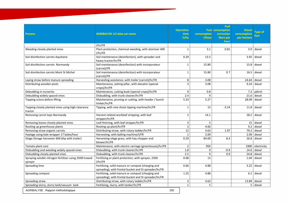
AGRIBALYSE : Rapport méthodologique 292
Process AGRIBALYSE LCI data set name Operation
time h/ha
Fuel consumption
l/hour
Fuel consumption
correction liters per
hour
Diesel consumption
per hectare
Type of fuel
l/hr/FR
Weeding closely planted vines Plant protection, chemical weeding, with atomiser 400 l/hr/FR
1 3.1 0.81 3.9 diesel
Soil disinfection carrots Aquitaine Soil maintenance (desinfection), with spreader and heavy tractor/hr/FR
0.29 13.5 3.92 diesel
Soil disinfection carrots Normandy Soil maintenance (desinfection) with incorporateur (carrot)/FR
1 15.80 15.8 diesel
Soil disinfection carrots Mont St Michel Soil maintenance (desinfection) with incorporateur (carrot)/FR
1 15.80 0.7 16.5 diesel
Laying straw before manure spreading Harvesting assistence, with trailer (carrot)/hr/FR 8 3.08 24.64 diesel
Distributing wooden posts Maintenance, setting pillar, with elevator (special crops)/hr/FR
3 3.08 9.24 diesel
Debudding in nurseries Maintenance, cutting buds (special crops)/hr/FR 9 0.8 7.2 pétrol
Debudding widely spaced vines Disbudding, with trunk cleaner/hr/FR 2.4 9 21.6 diesel
Topping scions before lifting Maintenance, pruning or cutting, with header / bunch limber/hr/FR
5.33 5.27 28.09 diesel
Topping closely planted vines using high clearance tractor
Tipping, with vine shoot tipping machine/hr/FR 1 15 -3.24 11.8 diesel
Removing carrot tops Normandy Harvest related workleaf stripping, with leaf stripper/hr/FR
2 14.1 28.2 diesel
Removing leaves closely planted vines Leaf thinning, with leaf stripper/hr/FR 3 5 15 diesel
Rooting up greenhouse plants Rooting up plant/hr/FR 2 4.60 9.2 diesel
Removing straw organic carrots Distributing straw, with rotary tedder/hr/FR 12 4.63 1.97 79.2 diesel
Haylage using bale wrapper 17 bales/hour Harvesting, with balling machine/t/FR 1 2.09 2.09 diesel
Silage (forage harvester 600 bhp with trailer) Harvesting silage grass, with hay chopper and blower/hr/FR
0.29 84.00 8.4 26.8 diesel
Tomato plant care Maintenance, with electric carriage (greenhouse)/hr/FR 2 950 1900 electricity
Disbudding and weeding widely spaced vines Disbudding, with trunk cleaner/hr/FR 1.8 9 -0.9 14.6 diesel
Disbudding closely planted vines Disbudding, with trunk cleaner/hr/FR 2.5 9 0.9 24.8 diesel
Spraying soluble nitrogen fertilizer using 2500l towed sprayer
Fertilizing or plant protection, with sprayer, 2500 l/hr/FR
0.08 13 1.04 diesel
Spreading lime Fertilizing, solid manure or compost (charging and spreading), with frontal bucket and 5t spreader/hr/FR
0.66 4.88 3.22 diesel
Spreading compost Fertilizing, solid manure or compost (charging and spreading), with frontal bucket and 5t spreader/hr/FR
1.25 4.88 6.1 diesel
Spreading straw Distributing straw, with rotary tedder/hr/FR 3 4.63 13.89 diesel
Spreading slurry, slurry tank/vacuum tank Fertilizing, slurry, with tanker/hr/FR 1 5 5 diesel

AGRIBALYSE : Rapport méthodologique 293
Process AGRIBALYSE LCI data set name Operation
time h/ha
Fuel consumption
l/hour
Fuel consumption
correction liters per
hour
Diesel consumption
per hectare
Type of fuel
Spreading slurry using trailing hoses 1500-2000 Fertilizing, slurry, with tanker/hr/FR 1 5 5 diesel
Spreading fertilizer carrots Aquitaine Fertilizing, solid manure (spreading only), with 8-10t spreader/hr/FR
0.25 8.70 -6.7 0.5 diesel
Spreading fertilizer organic carrots Normandy Fertilizing, with spreader, 2500 l/hr/FR 0.33 13 -6.33 2.2 diesel
Spreading fertilizer carrots Mont St Michel Fertilizing, with spreader, 2500 l/hr/FR 0.17 13 -6.53 1.1 diesel
Spreading fertilizer carrots Normandy Fertilizing, with spreader, 2500 l/hr/FR 0.25 13 -7.8 1.3 diesel
Spreading fertilizer under cover Fertilizing, with spreader/broadcaster, 500 l (orchard)/hr/FR
1.5 4.2 6.3 diesel
Spreading fertilizer using 2500l spreader Fertilizing, with spreader, 2500 l/hr/FR 0.12 13 1.56 diesel
Spreading manure Fertilizing, solid manure or compost (charging and spreading), with frontal bucket and 5t spreader/hr/FR
1.25 4.88 6.1 diesel
Spreading organic matter Fertilizing, solid manure or compost (charging and spreading), with frontal bucket and 5t spreader/hr/FR
1.25 4.88 6.1 diesel
Spreading straw organic carrots Fertilizing, solid manure or compost (charging and spreading), with frontal bucket and 5t spreader/hr/FR
8 4.88 39.04 diesel
Spreading fertilizer vine nursery Fertilizing, solid manure (charging and spreading) with 8-10t spreader/hr/FR
2.4 8.7 -0.63 19.4 diesel
Spreading fertilizer closely planted vines Fertilizing, solid manure (charging and spreading) with 8-10t spreader/hr/FR
0.75 8.7 1.17 7.4 diesel
Spreading fertilizer widely spaced vines Fertilizing, solid manure (charging and spreading) with 8-10t spreader/hr/FR
0.3 8.7 0.27 2.7 diesel
Spreading manure using spreader Fertilizing, solid manure (charging and spreading) with 8-10t spreader/hr/FR
1.33 8.70 11.57 diesel
Gasoline Plant protection, spraying, with knapsack sprayer/hr/FR 0.33 2.67 0.9 fuel
Laying straw organic carrots Distributing straw, with rotary tedder/hr/FR 2 4.63 2.19 13.64 diesel
Cutting the root stock Maintenance, pruning or cutting, with chopper blower/hr/FR
5.33 7.04 37.52 diesel
Cutting the root stock using secateurs Maintenance, cutting buds (special crops)/hr/FR 16 0.8 12.8 pétrol
Haylage swathing using 3m tedder Haying, with tedder/hr/FR 0.5 2 1 diesel
Mowing (7m mower, 300 bhp tractor) Mowing, with rotary mower 7m/hr/FR 0.19 22.26 4.23 diesel
Mowing, using mower conditioner Mowing, with rotary mower 3m/hr/FR 0.5 5.7 -3.1 1.3 diesel
Mowing, using 3m rotary mower Mowing, with rotary mower 3m/hr/FR 0.5 5.7 2.85 diesel
Applying average fertilizer to mangoes using sprayer Fertilizing or plant protection, with sprayer, 2500 l 0.42 5 2.1 diesel
Applying fertilizer to leaves using sprayer Fertilizing, with spreader/broadcaster, 500 l (orchard)/hr/FR
1 4.2 4.2 diesel
Fertilizing using 1500l spin spreader Fertilizing, with spreader, 2500 l/hr/FR 0.12 13 1.56 diesel

AGRIBALYSE : Rapport méthodologique 294
Process AGRIBALYSE LCI data set name Operation
time h/ha
Fuel consumption
l/hour
Fuel consumption
correction liters per
hour
Diesel consumption
per hectare
Type of fuel
Fertilizing using 500l spin spreader Fertilizing, with spreader, 2500 l/hr/FR 0.12 13 1.56 diesel
Tying up plants Maintenance, tying of plants, with binding machine (special crops)/hr/FR
5 1.00 5 diesel
Supplying growing medium Transporting of growing media, with trailer/p/FR 1 0.45 0.45 diesel
Rotary cultivator with roller Hoeing, with rotary hoe 3m/hr/FR 1.3 11.2 14.6 diesel
Rotary cultivator carrots Mont St Michel Soil maintenance, with rotary cultivator/hr/FR 2.5 41.2 103 diesel
Hoeing soil in nursery Hoeing, with 2 row hoe/hr/FR 4 6.17 -1.77 17.6 diesel
Hoeing closely planted vines Soil preparation (vine), with harrow/hr/FR 1.4 9.5 13.3 diesel
Hoeing widely spaced vines Soil preparation (vine), with harrow/hr/FR 1 9.5 9.5 diesel
Harrowing with 4m rotary harrow Harrowing, with rotary harrow (standard equipment)/hr/FR
0.7 14.3 10.01 diesel
Harrowing with rotary harrow and packer roller Harrowing, with rotary harrow (standard equipment)/hr/FR
0.7 14.3 10.01 diesel
Harrowing carrots after disinfection Harrowing, with rotary harrow (standard equipment)/hr/FR
0.33 14.3 5.4 6.5 diesel
Harrowing organic carrots Normandy Harrowing, with rotary harrow (standard equipment)/hr/FR
1 14.3 -1.1 13.2 diesel
Harrowing carrots Mont St Michel Harrowing, with rotary harrow (standard equipment)/hr/FR
1.33 14.3 2.17 21.91 diesel
Harrowing peach nursery Harrowing, with rotary harrow and packer (orchard)/hr/FR
2 13.85 27.7 diesel
Harrowing peach/apple nursery Harrowing, with rotary harrow and packer (orchard)/hr/FR
2 13.85 27.7 diesel
Harrowing apple nursery Harrowing, with rotary harrow and packer (orchard)/hr/FR
2 13.85 27.7 diesel
Harrowing under cover Harrowing, with rotary harrow and packer (orchard)/hr/FR
5 13.85 -6.15 38.5 diesel
Harrowing cider apple orchard Harrowing, with small tractor (orchard)/hr/FR 1 9.20 4.88 14.08 diesel
12m chain harrow Harrowing, with harrow 12m/hr/FR 0.11 10.8 1.19 diesel
Platform working (hour) Maintenance, with platform self-propelled (special crops)/hr/FR
1 1.17 1.17 electricity
Tractor and compressor (hour) Maintenance, with compressor (special crops)/hr/FR 1 3.10 3.1 diesel
Sinking posts for training wires Maintenance, pillar installation, with post hole digger (special crops)/hr/FR
2.5 5.28 13.2 diesel
Hoeing between closely planted vines Hoeing, with 2 row hoe/hr/FR 2.1 4.4 9.54 29.3 diesel
Hoeing between widely spaced vines Hoeing, with 2 row hoe/hr/FR 1.2 4.4 9.54 16.7 diesel
Plowing Ploughing (vine), with frame plough/hr/FR 1.5 8 10.8 28.2 diesel

AGRIBALYSE : Rapport méthodologique 295
Process AGRIBALYSE LCI data set name Operation
time h/ha
Fuel consumption
l/hour
Fuel consumption
correction liters per
hour
Diesel consumption
per hectare
Type of fuel
Plowing with 5 furrow plow Ploughing, with 5 or 6 soc plough/hr/FR 1.33 18.75 24.9 diesel
Plowing before planting orchard Ploughing, in orchard/hr/FR 1 16.15 -2.07 14.08 diesel
Plowing with vineyard plow - vine nursery Ploughing (vine), with frame plough/hr/FR 1.45 8 11.6 diesel
Plowing carrots Aquitaine Ploughing, with 8 soc plough/hr/FR 0.5 24.60 12.3 diesel
Plowing organic carrots Normandy Ploughing, with 5 or 6 soc plough/hr/FR 1 18.75 2.35 21.1 diesel
Plowing carrots Mont St Michel Ploughing, with 5 or 6 soc plough/hr/FR 0.67 18.75 4.39 15.5 diesel
Plowing carrots Normandy Ploughing, with 4 soc plough/hr/FR 1 15.80 15.8 diesel
Plowing peach nursery Ploughing, in orchard/hr/FR 2 16.15 32.3 diesel
Plowing peach/apple nursery Ploughing, in orchard/hr/FR 2 16.15 32.3 diesel
Plowing apple nursery Ploughing, in orchard/hr/FR 2 16.15 32.3 diesel
Subsoiling orchard Ploughing, with 1 soc plough/hr/FR 3 24.67 74.01 diesel
Plowing widely spaced vines Ploughing (vine), with frame plough/hr/FR 1.4 8 1.35 13.1 diesel
Plowing, 4 furrow plow Ploughing, with 5 or 6 soc plough/hr/FR 1.4 18.75 26.25 diesel
Land preparation - Dry Soil preparation, with disc harrow/hr/FR 3 4.24 12.72 pétrol
Land preparation - Humid Soil preparation, with disc harrow/hr/FR 2.5 4.24 10.6 pétrol
Land preparation post sowing Soil preparation, with rotary tiller/hr/FR 2.5 4.24 10.6 pétrol
Land preparation pre sowing Soil preparation, with rotary tiller/hr/FR 2.5 4.24 10.6 pétrol
Handling potato plants Maintenance, with forklift truck/hr/FR 0.86 20.77 17.86 diesel
Flooding paddy fields (3.5h) Flooding of paddy fields, with motor cultivator/hr/FR 3.5 0.64 2.24 pétrol
Flooding paddy fields (11h) Flooding of paddy fields, with motor cultivator/hr/FR 11 0.64 7.04 pétrol
Flooding paddy fields (7h) Flooding of paddy fields, with motor cultivator/hr/FR 7 0.64 4.48 pétrol
Heeling in and removing scions Sowing or planting, maiden tree, with ditcher/hr/FR 20 7.04 140.8 diesel
Harvesting cereals using combine harvester200 bhp Harvesting, with combine harvester/hr/FR 0.67 25.60 17.15 diesel
Earthing up organic carrots Normandy Earthing up, with 2 row hoe/hr/FR 1.5 21.00 -3.4 26.4 diesel
Earthing up carrots Mont St Michel Earthing up, with how (carrot)/hr/FR 1.33 6.15 4.82 14.59 diesel
Earthing up carrots Normandy Earthing up, with how (carrot)/hr/FR 2 6.15 12.3 diesel
Digging and closing trench for drip irrigation Tillage, preparation irrigation/hr/FR 3 7.70 23.1 diesel
Sinking posts for training Indentation of pots, with tractopelle/hr/FR 2.66 20.00 53.2 diesel
Planting and earthing up potatoes, planter and 4 row lister
Sowing or planting and earthing up, potato, with 4-row-planter and 2 row how/hr/FR
0.9 20.00 18 diesel
Sinking training wire posts nursery Maintenance, setting pillar for tying in (special crops)/hr/FR
2.66 3.53 9.39 diesel
Sinking training wire posts apple trees Maintenance, setting pillar for tying in (special crops)/hr/FR
4 3.53 1.75 21.12 diesel
Layering apple trees Sowing or planting, trees (orchard)/hr/FR 20 5.61 112.2 diesel
Planting peach rootstock Sowing or planting, trees (orchard)/hr/FR 16 5.61 89.76 diesel

AGRIBALYSE : Rapport méthodologique 296
Process AGRIBALYSE LCI data set name Operation
time h/ha
Fuel consumption
l/hour
Fuel consumption
correction liters per
hour
Diesel consumption
per hectare
Type of fuel
Sinking posts for closely planted vines before tying up Maintenance, setting pillar for tying in (special crops)/hr/FR
8 3.5 0.87 34.9 diesel
Sinking posts for widely spaced vines before tying up Maintenance, setting pillar for tying in (special crops)/hr/FR
3 3.5 0.87 13.1 diesel
Planting potatoes using 4 row planter Sowing or planting, potato, with 4-row-planter/hr/FR 1 17.20 17.2 diesel
Planting rootstock nursery Sowing or planting, trees (orchard)/hr/FR 14 5.61 5.61 157.08 diesel
Planting cider apple orchard Sowing or planting, trees (orchard)/hr/FR 1.25 5.61 1.43 8.8 diesel
Laying mulching film on two rows of vines with plastic nursery
Maintenance, soil covering with plastic (grafted vine plants)/hr/FR
3 8 24 diesel
Ploughing Ploughing, with 5 or 6 soc plough/hr/FR 0.87 18.75 -5.56 11.48 diesel
Sinking stakes in nursery Maintenance, rooting up maiden tree, with elevator (special crops)/hr/FR
8 3.52 28.16 diesel
Fitting and removing training wires in nursery Maintenance, with rolling off device, heavy tractor (special crops)/hr/FR
12 2.64 31.68 diesel
Pushing prunings Pushing wood, with small tractor/hr/FR 5 1.1 5.5 diesel
Preparing carrot beds Aquitaine Soil decompactation, with cultivator/hr/FR 1 26.40 26.4 diesel
Preparing seed beds Harrowing, with small tractor (orchard)/hr/FR 1 9.20 9.2 diesel
Preparing apple tree beds Harrowing, with small tractor (orchard)/hr/FR 1.25 9.20 11.5 diesel
Preparing soil for planting orchard Tillage, ploughing, tree nursery/hr/FR 0.83 7.70 6.39 diesel
Preparing soil for planting apple orchard Tillage, ploughing, tree nursery/hr/FR 1.04 7.70 8.01 diesel
Preparing soil for drip irrigation trench Maintenance, preparation soil for irrigation channel, with rotary hoe (special crops)/hr/FR
3 7.93 23.79 diesel
Baling hay (4t DM/ha) with round baler Baling, with round baler (straw)/ha/FR 1 11.7 11.7 diesel
Preliminary pruning widely spaced vine Preliminary pruning, with pruning machine/hr/FR 1.5 22 33 diesel
Preliminary pruning closely planted vine Preliminary pruning, with pruning machine/hr/FR 2 22 44 diesel
Applying pesticide under cover using sprayer Plant protection, spraying, with self-propelled atomiser/hr/FR
2.5 4.60 11.5 diesel
Applying pesticide using 1200l sprayer Plant protection, spraying, with sprayer, 1200 l/hr/FR 0.11 12.22 1.34 diesel
Applying pesticide using 2500l sprayer Fertilizing or plant protection, with sprayer, 2500 l/hr/FR
0.08 13.00 1.04 diesel
Applying pesticide using 800l sprayer attachment nursery
Plant protection, chemical weeding, with atomiser 400 l/hr/FR
1 6.15 6.15 diesel
Minimum tillage, using 13 shank chisel plow attachment
Soil decompactation, with 4.5m chisel/hr/FR 0.63 25.00 15.75 diesel
400l sprayerattachment for vine nursery Plant protection, spraying, with atomiser/sprayer, 2000 l/hr/FR
1 8.8 5.58 14.4 diesel

AGRIBALYSE : Rapport méthodologique 297
Process AGRIBALYSE LCI data set name Operation
time h/ha
Fuel consumption
l/hour
Fuel consumption
correction liters per
hour
Diesel consumption
per hectare
Type of fuel
Spraying for rooting up Plant protection, spraying, with atomiser/sprayer, 2000 l/hr/FR
2 8.8 5.58 28.8 diesel
Spraying closely planted vines Plant protection, spraying, with atomiser/sprayer, 2000 l/hr/FR
1 8.8 3.78 12.6 diesel
Spraying widely spaced vines Plant protection, spraying, with atomiser/sprayer, 2000 l/hr/FR
0.5 8.8 5.13 7 diesel
Collecting forage using self-propelled harvester Harvesting silage grass, with hay chopper and blower/hr/FR
0.5 84.00 42 diesel
Harvesting carrots Créances Harvesting, 1 row puller/hr/FR 11 8.80 96.8 diesel
Harvesting winter carrots Aquitaine using self-propelled harvester
Harvesting, with complete harvester (carrot)/hr/FR 4 17.60 70.4 diesel
Harvesting winter carrots Aquitaine using towed harvester
Harvesting, 3 row puller/hr/FR 4 14.08 56.32 diesel
Harvesting winter carrots Mont St Michel Harvesting, 1 row puller/hr/FR 14 8.80 123.2 diesel
Harvesting fall carrots Val de Saire Harvesting, 1 row puller/hr/FR 15 8.80 132 diesel
Harvesting winter carrots Val de Saire Harvesting, 1 row puller/hr/FR 17.5 8.80 154 diesel
Harvesting sugarbeet using 1 tractor for topping, lifting and loading 6 rows
Harvesting, with tractor an 6 row rooting up (beets)/hr/FR
1.3 25.00 32.5 diesel
Harvesting sugarbeet using 6 row self-propelled harvester + 1 or 2 trailers
Harvesting, with complete harvester (6 row) and trailers (beets)/hr/FR
1 40.00 40 diesel
Harvesting sugar beet with 6 row self propelled combine harvester
Harvesting, with complete harvester (beets)/hr/FR 1 40.00 40 diesel
Harvesting clementines Harvesting, with trailer (clementine)/hr/FR 9 3.52 31.68 diesel
Lifting potatoes using harvester Harvesting, with complete harvester (potatoes)/hr/FR 2 16 32 diesel
Harvesting cider apples using harvester Harvesting, with harvester (fruits)/hr/FR 3 14.08 42.24 diesel
Harvesting rice Harvesting, with combine harvester/hr/FR 0.83 25.6 21.25 diesel
Collecting and transporting carrots Créances Harvesting assistence, with trailer (carrot)/hr/FR 11 3.08 33.88 diesel
Collecting and transporting fall carrots Mont St Michel Harvesting assistence, with trailer (carrot)/hr/FR 12.5 3.08 38.5 diesel
Collecting and transporting winter carrots Mont St Michel
Harvesting assistence, with trailer (carrot)/hr/FR 14 3.08 43.12 diesel
Collecting and transporting fall carrots Val de Saire Harvesting assistence, with trailer (carrot)/hr/FR 15 3.08 46.2 diesel
Collecting and transporting winter carrots Val de Saire Harvesting assistence, with trailer (carrot)/hr/FR 17.5 3.08 53.9 diesel
Collecting and transporting carrots Aquitaine Harvesting assistence, with trailer (21 t)/hr/FR 2.5 7.05 17.63 diesel
Collecting and transporting winter carrots Aquitaine Harvesting assistence, with trailer (21 t)/hr/FR 4 7.05 28.2 diesel
Repotting Repotting, with potting machine/hr/FR 1 0.45 0.45 electricity
Plowing apple orchard Soil decompactation, with 4.5m chisel/hr/FR 0.63 25 15.75 diesel

AGRIBALYSE : Rapport méthodologique 298
Process AGRIBALYSE LCI data set name Operation
time h/ha
Fuel consumption
l/hour
Fuel consumption
correction liters per
hour
Diesel consumption
per hectare
Type of fuel
Turning carrots for storage Mont St Michel Preparation of soil, with plough (before carrot harvest)/hr/FR
3 15.8 -5.23 31.71 diesel
Turning carrots for storage Aquitaine Preparation of soil, with plough (before carrot harvest)/hr/FR
1 15.80 15.8 diesel
Removing training wires before rooting up apple orchard
Maintenance, with rolling off device (special crops)/hr/FR
6 0.4 2.4 pétrol
Trimming vines in nursery using tractor Tipping, with vine shoot tipping machine/hr/FR 3.6 15 54 diesel
Trimming closely planted vines Tipping, with vine shoot tipping machine/hr/FR 1.4 15 21 diesel
Trimming widely spaced vines Tipping, with vine shoot tipping machine/hr/FR 1 15 -3.24 11.8 diesel
Rotavator carrots Normandy Hoeing, with rotary hoe 3m/hr/FR 0.4 13.25 5.3 diesel
Rotavator under cover Hoeing, with rotary hoe (greenhouse)/hr/FR 7 7.70 53.9 diesel
Spader under cover Hoeing, with rotobêche/hr/FR 7 7.70 53.9 diesel
Rolling using 3m corrugated roller Rolling, with roller 3m/hr/FR 0.59 4.20 2.48 diesel
Rolling using 9m roller Rolling, with roller 9m/hr/FR 0.2 15.00 3 diesel
Rolling soil before planting closely planted vines Rolling, with roller 9m/hr/FR 1 10 -4.5 5.5 diesel
Shaking trees for harvesting Shaking, with shaker (orchard)/hr/FR 1 8.80 8.8 diesel
Drilling using standard 4m drill Sowing or planting, with classic seeder and harrow/hr/FR
1.3 12 15.6 diesel
Drilling carrots Aquitaine Sowing or planting, with 3 row seeder (carrot)/hr/FR 1 7.90 7.9 diesel
Drilling organic carrots Normandy Sowing or planting, with pneumatic seeder (carrot)/hr/FR
1.5 6.16 2.64 13.2 diesel
Drilling carrots Normandy Sowing or planting, with pneumatic seeder (carrot)/hr/FR
2.5 6.16 15.4 diesel
Combine drill, mechanical Sowing or planting, with classic seeder and harrow/hr/FR
0.83 16.83 13.97 diesel
Combine drill, drill, seed on demand Sowing or planting, with pneumatic seeder and harrow/hr/FR
0.83 16.83 13.97 diesel
Sowing no till, 4m disk drill Sowing or planting, direct seeding/hr/FR 0.42 14.29 6 diesel
Sowing grass in orchard Sowing or planting, grass (orchard)/hr/FR 1 6.16 6.16 diesel
Sowing grass in apple orchard Sowing or planting, grass (orchard)/hr/FR 1.25 6.16 7.7 diesel
Sowing with pneumatic seed-on-demand drill Sowing or planting, with pneumatic seeder, 6 rows/hr/FR
0.67 13.47 9.02 diesel
Removing scions from nursery Maintenance, rooting up maiden tree, with elevator (special crops)/hr/FR
20 3.52 70.4 diesel
Removing scions from nursery Maintenance, rooting up maiden tree, with elevator (special crops)/hr/FR
20 3.52 70.4 diesel

AGRIBALYSE : Rapport méthodologique 299
Process AGRIBALYSE LCI data set name Operation
time h/ha
Fuel consumption
l/hour
Fuel consumption
correction liters per
hour
Diesel consumption
per hectare
Type of fuel
Decompacting soil using subsoiler Soil decompactation, with subsoil plow 2m/hr/FR 2 13 1.8 29.6 diesel
Subsoiling carrots Mont St Michel Soil decompactation/hr/FR 0.67 17.69 5.44 15.5 diesel
Subsoiling carrots Normandy Soil decompactation, with subsoil plow 2m/hr/FR 1 13.00 5.5 18.5 diesel
Subsoiling under cover Soil decompactation, with subsoil plow 2m/hr/FR 3 13.00 39 diesel
Subsoiling using subsoiler Soil decompactation, with subsoil plow 2m/hr/FR 2 13 26 diesel
Subsoiling for mangoes Soil decompactation, with subsoil plow 2m/hr/FR 1.5 13 6.3 29 diesel
Pruning cider apple orchard Maintenance, pruning or cutting, with chain saw/hr/FR 15 0.48 7.2 pétrol
Pruning cider apple orchard (trimming) Maintenance, pruning, with angle mower/hr/FR 6 8.8 52.8 diesel
Compacting silage Silage plat, settling for silage with 2 tractors/hr/FR 0.61 11.53 7.03 diesel
Tillage / Rolling Rolling, with roller 9m/hr/FR 0.33 15 4.95 diesel
Cutting grass in orchard Plant protection, weeding, with rotary beater/hr/FR 0.75 4.62 3.47 diesel
Cutting grass in apple orchard Plant protection, weeding, with rotary beater/hr/FR 0.94 4.62 4.34 diesel
Cutting grass between rows in cider apple orchard Plant protection, weeding, with mower/hr/FR 0.9 4.7 4.23 diesel
Cutting grass between rows closely planted vines Plant protection, weeding, with mower/hr/FR 2 4.7 4.77 18.9 diesel
Manual herbicide spraying Plant protection, spraying, with knapsack sprayer/hr/TH 3 11.7 35.1 diesel
Manual insecticide spraying Plant protection, spraying, with knapsack sprayer/hr/TH 3 0.5 1.5 diesel
Applying pesticide to citrus fruit to protect against fruit flies using lance sprayer
Plant protection, chemical weeding, with atomiser 400 l/hr/FR
3 3.1 9.3 diesel
Applying pesticides to citrus fruit to protect against leaf miners and ceratitis capitata (Mediterranean fruit fly)
Plant protection, chemical weeding, with atomiser 400 l/hr/FR
1 3.1 3.1 diesel
Applying average pesticides for mangoes Fertilizing or plant protection, with sprayer, 2500 l/hr/FR
0.42 13 -7.2 2.4 diesel
Applying pesticide under cover Plant protection, spraying, with atomiser (greenhouse)/hr/FR
4 1.76 7.04 diesel
Applying pesticide peach orchard Plant protection, spraying, with atomiser/sprayer, 2000 l/hr/FR
0.5 8.80 4.4 diesel
Applying pesticide apply orchard Plant protection, spraying, with atomiser/sprayer, 2000 l/hr/FR
0.75 8.80 -2.64 4.62 diesel
Spraying cider apple orchard Plant protection, spraying, with trailed atomizer, 2000l/hr/FR
0.67 8.80 5.9 diesel
Applying pesticide carrots Aquitaine Plant protection, chemical weeding, with self-propelled machine/hr/FR
0.1 12.00 1.2 diesel
Applying pesticide carrots Normandy Plant protection, spraying, with sprayer, 1200 l/hr/FR 0.5 12.22 -4.22 4 diesel
Transporting cases for tomatoe harvest Harvesting assistence, with trailer (carrot)/hr/FR 8 3.08 24.64 diesel
Transporting grain 140 bhp trailer 2 axle 15 t Transporting to farm, with 2 axle trailer (15 t)/hr/FR 0.67 13.34 8.94 diesel

AGRIBALYSE : Rapport méthodologique 300
Process AGRIBALYSE LCI data set name Operation
time h/ha
Fuel consumption
l/hour
Fuel consumption
correction liters per
hour
Diesel consumption
per hectare
Type of fuel
Transporting grain 160 bhp 2 axle 15 t Transporting to farm, with 2 axle trailer (15 t)/hr/FR 0.67 13.34 2 10.28 diesel
Transporting forage 110 bhp trailer 2 axle 15 t Transporting to farm, with trailer (<15t) heavy tractor/hr/FR
0.59 12.10 7.14 diesel
Transporting forage 90 bhp forage flatbed trailer 2 axle 10-02 t
Transporting, with forage flatbed/hr/FR 0.4 9.90 3.96 diesel
Transporting maize forage 110 bhp trailer 2 axle 15 t Transporting to farm, with trailer (<15t) heavy tractor/hr/FR
1.25 12.1 15.13 diesel
Transporting maize grain 100 bhp trailer 2 axle 12-14 t Transporting to farm, with trailer (<15t) heavy tractor/hr/FR
1 12.1 -1.2 10.9 diesel
Transporting potatoes 135 bhp trailer 2 axle 16-18 t Transporting to farm, with trailer (<15t) heavy tractor/hr/FR
2.5 12.1 2.9 37.5 diesel
Preparing soil before planting closely planted vines Harrowing, 3m harrow/hr/FR 2 10 20 diesel
Preparing soil between rows (every row) Hoeing, with 4-6m hoe (standard)/hr/FR 0.33 15 4.95 diesel
Preparing soil for changing plastic tunnel film north Hoeing, with rotary hoe/hr/FR 1 7.7 7.7 diesel
Preparing soil for changing plastic tunnel film south Hoeing, with rotary hoe/hr/FR 1.5 7.7 11.55 diesel
Superficial hoeing widely spaced vines Hoeing, with rotary hoe 3m/hr/FR 1.3 13.3 0.23 17.6 diesel
Harvesting grapes from closely planted vines Harvesting (vine), with trailer/hr/FR 2.14 30 64.2 diesel
harvesting grapes from widely spaced vines Harvesting (vine), with trailer/hr/FR 1.6 30 48 diesel
Spring tine harrow, 3m Harrowing, with vibrating tine cultivator (standard equipment) 5m/hr/FR
0.34 15 5.1 diesel
Spring tine harrow 5m Harrowing, with vibrating tine cultivator (standard equipment) 5m/hr/FR
0.34 15 5.1 diesel
Spring tine harrow organic carrots Harrowing, with vibrating tine cultivator 6m/hr/FR 1 15 15 diesel

AGRIBALYSE®: Methodology 301
Appendix L: Building the livestock feed processes
1. Method
AGRIBALYSE “feed ingredients” LCIs comre from ECOALIM project (IFIP 2016). Those LCIs provide benchmark values for « raw ingredients” (wheat, corn etc.) used by livestocks in France. Those ingredients are combined to make “composed feeds” (ex : bovine feeds), corresponding to the physiological needs of each type of animals, and evolving following their physiological phase. The methodology to build those animal “feed ingredients” LCIs is very similar to other AGRIBALYSE crops, provided in “plant production” folder. However a few differences must be noted : including the seeds, ammoniac emission model or the way for accounting the agronomic rotation. All feeds used Ecoinvent v3.2 in background, except for a few processus (ex : fish feed), where no unit process data was available (AGRIBALYSE 2016). More methodological detail will be provided once Ecoalim project will be finalized. For human food, it is recommended to use in priority crops in “Plant production” folder, wereas for animal feeds, users should use “Animal Feed” folder. Transport models Several transport models were considered. Raw materials All raw materials must be transported to the feed mix fabrication plant. All raw material production processes used are “at field gate” or “at factory”. For raw materials produced in France, it was assumed that the location of the feed fabrication plant was not known. Consequently, the same means of transport and the same distances were taken into account for all raw materials, whether their production zone was known or not. The average transport distances and means of transport were defined according to Nguyen et al (2012). For raw materials imported from abroad, the distances and means of transport between the place of production and France defined in GESTIM (Gac et al, 2010) were taken into account. The distances and means of transport to France were then added using the methodology described above. Table 160 gives the distances and means of transport and the processes used Table 160: Transport models for raw materials from the place of production to the feed fabrication plant Source of
RM Means of transport
Distance transported (km)
Process Source
database
France Road 110 Transport, lorry >32t, EURO3/RER U
ecoinvent
France Rail 390 Transport, freight, rail/RER U ecoinvent
Imported Road According to GESTIM Transport, lorry >32t, EURO3/RER U
ecoinvent
Imported Rail According to GESTIM Transport, freight, rail/RER U ecoinvent
Imported Sea According to GESTIM Transport, transoceanic freight ecoinvent

AGRIBALYSE®: Methodology 302
ship/OCE U
Feed mixes Feed mixes must be transported from the feed fabrication plant to the farm where they will be consumed by the animals. The assumption described in GESTIM was used: road transport for a distance of 130 km. The process used was “Transport, lorry >32t, EURO3/RER U” (ecoinvent). Production on the farm Some feed mixes are made directly on the farm, using some raw materials produced on the farm. The following assumptions were taken into account:
No transport for the raw materials produced on the farm
Distances and means of transport the same as those used for transport between the place of production and the feed fabrication plant for raw materials not produced on the farm
2. Feed mixes
Fabrication process The energy required to produce the feed mixes was taken into account. The data was taken from the Tecaliman report (1995-1997 and 2009). Table 161 gives the data used. These energy requirements were taken into account for both feed production on the farm and feed production in a factory. Table 161: Energy requirements for producing one tonne of feed mix
Type of power Energy (kWh) Process Source
database
Electricity 41 Electricity, medium voltage, production FR, at grid/FR U
ecoinvent
Heat 20.5 Heat, natural gas, at industrial furnace >100kW/RER U
ecoinvent
Building the LCIs for producing feed mixes on the farm Several feed mixes are produced completely or partially on the farm. The LCIs were built in the same way for feed mixes produced 100% on the farm as for commercially produced feed. Only the assumptions on transport were modified (see above). The following procedure was used for feed mixes produced partially on the farm and partly in a factory: i) feed data set built using the “produced at factory” transport model; ii) feed data set built using the “produced at the farm” transport model and iii) final feed data set built using a given percentage of each of the feed data sets already built. Composition of feed mixes Table 162 to Table 165 give the composition of AGRIBALYSE feed mix LCI data sets. The abbreviation OFP stands for “on-farm processed”

AGRIBALYSE®: Methodology 303
Table 162: Feed mix processes for pig production in AGRIBALYSE. Feed mix formulation
SimaPro process Raw material % composition Comments
Sow,rapeseed meal based feed,gestating feed,conv prod, at farm gate
Soft wheat 31.3 Barley 30 Grain maize 3.3 Soft wheat bran 15 Soft wheat middlings 3.6 Protein peas 5 Rapeseed cake 3.2 Sunflower cake with hulls 2.2 Dried sugar beet pulp 3 Calciuim carbonate 2.13 Dicalcium phosphate 0.16 Salt (NaCl) 0.4 L-Lysine HCl 0.15 L-Threonine 0.04
Sow,rapeseed meal based feed,lactating feed,conv prod, at farm gate
Soft wheat 41 Barley 15 Grain maize 2.3 Soft wheat middlings 10.2 Protein peas 12.2 Soybean cake 3 Rapeseed cake 12 Rapeseed 0.9 Calciuim carbonate 1.49 Dicalcium phosphate 0.65 Salt (NaCl) 0.4 L-Lysine HCl 0.26 DL Methionine 0.02 L-Threonine 0.07
Weaned piglet,rapeseed meal based feed,WP 1st phase feed,conv prod, at farm gate
Soft wheat 41.9 Grain maize 20 Soybean cake 15.3 Potato protein concentrate 3 Soybean concentrate 3 Whey powder, with lactose 10 Palm oil 2.6 Calciuim carbonate 1.01 Dicalcium phosphate 1.33 Salt (NaCl) 0.3 L-Lysine HCl 0.56 DL Methionine 0.22 L-Threonine 0.22 L-Tryptophane 0.06
Weaned piglet,rapeseed meal based feed,WP 2nd phase feed,conv prod, at farm gate
Soft wheat 60 Soft wheat middlings 2.8 Protein peas 13.8 Soybean cake 6.5 Rapeseed cake 12 Rapeseed 1.5 Calciuim carbonate 1.04 Dicalcium phosphate 0.7 Salt (NaCl) 0.4 L-Lysine HCl 0.47 DL Methionine 0.09 L-Threonine 0.16 L-Tryptophane 0.03
Pig,rapeseed meal based feed,growing feed,conv prod, at farm gate
Soft wheat 69.1 Soft wheat middlings 1.3 Protein peas 7.1 Rapeseed cake 15 Sunflower cake with hulls 4.3

AGRIBALYSE®: Methodology 304
SimaPro process Raw material % composition Comments
Rapeseed 0.6 Calciuim carbonate 1.25 Salt (NaCl) 0.3 L-Lysine HCl 0.41 DL Methionine 0.02 L-Threonine 0.11 L-Tryptophane 0.01
Pig,rapeseed meal based feed,finishing feed,conv prod, at farm gate
Soft wheat 71.7 Barley 8 Protein peas 1.9 Rapeseed cake 11 Sunflower cake with hulls 5 Calciuim carbonate 1.07 Salt (NaCl) 0.3 L-Lysine HCl 0.42 DL Methionine 0.01 L-Threonine 0.1
Sow,soybean meal based feed,gestating feed,conv prod, at farm gate
Soft wheat 21.2 Barley 30 Grain maize 10 Soft wheat bran 15 Soft wheat middlings 9.2 Soybean cake 4.7 Dried sugar beet pulp 6.5 Calciuim carbonate 2.07 Dicalcium phosphate 0.24 Salt (NaCl) 0.4 L-Lysine HCl 0.13 L-Threonine 0.04
Sow,soybean meal based feed,lactating feed,conv prod, at farm gate
Soft wheat 29.7 Barley 18.1 Grain maize 17.9 Grain maize, moist 15 Soybean cake 15.7 Calciuim carbonate 1.51 Dicalcium phosphate 0.86 Salt (NaCl) 0.4 L-Lysine HCl 0.24 DL Methionine 0.02 L-Threonine 0.06
Weaned piglet,soybean meal based feed,WP 1st phase feed,conv prod, at farm gate
Soft wheat 41.9 Grain maize 20 Soybean cake 15.3 Potato protein concentrate 3 Soybean concentrate 3 Whey powder, with lactose 10 Palm oil 2.6 Calciuim carbonate 1.01 Dicalcium phosphate 1.33 Salt (NaCl) 0.3 L-Lysine HCl 0.56 DL Methionine 0.22 L-Threonine 0.22 L-Tryptophane 0.06
Weaned piglet,soybean meal based feed,WP 2nd phase feed,conv prod, at farm gate
Soft wheat 61.2 Barley 10 Soft wheat middlings 4.7 Soybean cake 20.5 Calciuim carbonate 1.03 Dicalcium phosphate 1.03 Salt (NaCl) 0.4 L-Lysine HCl 0.41

AGRIBALYSE®: Methodology 305
SimaPro process Raw material % composition Comments
DL Methionine 0.09 L-Threonine 0.13 Soft wheat 71.4
Pig,soybean meal based feed,growing feed,conv prod, at farm gate
Soft wheat bran 8 Soft wheat middlings 2 Soybean cake 9.3 Rapeseed cake 5 Sunflower cake with hulls 1.7 Calciuim carbonate 1.26 Salt (NaCl) 0.3 L-Lysine HCl 0.39 DL Methionine 0.03 L-Threonine 0.11
Pig,soybean meal based feed,finishing feed,conv prod, at farm gate
Soft wheat 61 Barley 13.4 Soft wheat bran 7.4 Protein peas 4.2 Soybean cake 3.6 Rapeseed cake 5 Sunflower cake with hulls 3 Calciuim carbonate 1.09 Salt (NaCl) 0.3 L-Lysine HCl 0.37 DL Methionine 0.03 L-Threonine 0.11
Sow,on-farm feed supply,gestating feed,conv prod, at farm gate
Soft wheat 45.64 100% OFP with local RM Barley 36.36 100% OFP with local RM Rapeseed cake 8.4 100% OFP Sunflower cake with hulls 6 100% OFP Calciuim carbonate 2.17 100% OFP Dicalcium phosphate 0.362 100% OFP Salt (NaCl) 0.4 100% OFP L-Lysine HCl 0.152 100% OFP L-Threonine 0.005 100% OFP
Sow,on-farm feed supply,lactating feed,conv prod, at farm gate
Soft wheat 60 100% OFP with local RM Barley 14.7 100% OFP with local RM Soybean cake 7 100% OFP Rapeseed cake 10 100% OFP Sunflower cake with hulls 4.66 100% OFP Calciuim carbonate 1.416 100% OFP Dicalcium phosphate 0.858 100% OFP Salt (NaCl) 0.4 100% OFP L-Lysine HCl 0.326 100% OFP L-Threonine 0.07 100% OFP
Weaned piglet,on-farm feed supply,WP 1st phase feed,conv prod, at farm gate
Soft wheat 41.9 Grain maize 20 Soybean cake 15 Potato protein concentrate 3 Soybean concentrate 3 Whey powder, with lactose 10 Palm oil 2.6 Calciuim carbonate 1.01 Dicalcium phosphate 1.33 Salt (NaCl) 0.3 L-Lysine HCl 0.56 DL Methionine 0.22 L-Threonine 0.22 L-Tryptophane 0.06
Weaned piglet,on-farm feed supply,WP 2nd phase feed,conv prod, at farm gate
Soft wheat 59.12 100% OFP with local RM Barley 15 100% OFP with local RM Soybean cake 18 100% OFP Rapeseed cake 3.44 100% OFP

AGRIBALYSE®: Methodology 306
SimaPro process Raw material % composition Comments
Palm oil 0.16 100% OFP Calciuim carbonate 1.3 100% OFP Dicalcium phosphate 0.988 100% OFP Salt (NaCl) 0.4 100% OFP L-Lysine HCl 0.434 100% OFP DL Methionine 0.084 100% OFP L-Threonine 0.135 100% OFP L-Tryptophane 0.01 100% OFP
Pig,on-farm feed supply,growing feed,conv prod, at farm gate
Soft wheat 41.86 100% OFP with local RM Barley 10 100% OFP with local RM Grain maize, moist 25 100% OFP with local RM Soybean cake 14 100% OFP Rapeseed cake 6.3 100% OFP Calciuim carbonate 1.384 100% OFP Dicalcium phosphate 0.234 100% OFP Salt (NaCl) 0.4 100% OFP L-Lysine HCl 0.332 100% OFP DL Methionine 0.027 100% OFP L-Threonine 0.089 100% OFP L-Tryptophane 0.004 100% OFP
Pig,on-farm feed supply,finishing feed,conv prod, at farm gate
Soft wheat 44.86 100% OFP with local RM Barley 10 100% OFP with local RM Grain maize, moist 25 100% OFP with local RM Soybean cake 6 100% OFP Rapeseed cake 12 100% OFP Calciuim carbonate 1.15 100% OFP Dicalcium phosphate 0.1 100% OFP Salt (NaCl) 0.4 100% OFP L-Lysine HCl 0.356 100% OFP DL Methionine 0.004 100% OFP L-Threonine 0.082 100% OFP L-Tryptophane 0.006 100% OFP
Sow,excess slurry treatment,gestating feed,conv prod, at farm gate
Soft wheat 33.4 Barley 24.56 Grain maize 6.64 Soft wheat bran 11 Soft wheat middlings 4.74 Protein peas 4.72 Rapeseed cake 1.05 Sunflower cake, partially dehulled
1.1
Sunflower cake with hulls 5.9 Dried sugar beet pulp 3 Molasses from sugarcane 0.8 Calciuim carbonate 2.146 Dicalcium phosphate 0.238 Salt (NaCl) 0.4 L-Lysine HCl 0.164 L-Threonine 0.042
Sow,excess slurry treatment,lactating feed,conv prod, at farm gate
Soft wheat 43.56 Barley 18 Grain maize 4.34 Soft wheat bran 5 Soft wheat middlings 4.96 Protein peas 3 Soybean cake 8.92 Rapeseed cake 8.16 Rapeseed 0.76 Molasses from sugarcane 0.12 Calciuim carbonate 1.542 Dicalcium phosphate 0.74 Salt (NaCl) 0.4

AGRIBALYSE®: Methodology 307
SimaPro process Raw material % composition Comments
L-Lysine HCl 0.278 DL Methionine 0.017 L-Threonine 0.07
Weaned piglet,excess slurry treatment,WP 1st phase feed,conv prod, at farm gate
Soft wheat 41.9 Grain maize 20 Soybean cake 15.3 Potato protein concentrate 3 Soybean concentrate 3 Whey powder, with lactose 10 Palm oil 2.6 Calciuim carbonate 1.01 Dicalcium phosphate 1.33 Salt (NaCl) 0.3 L-Lysine HCl 0.56 DL Methionine 0.22 L-Threonine 0.22 L-Tryptophane 0.06
Weaned piglet,excess slurry treatment,WP 2nd phase feed,conv prod, at farm gate
Soft wheat 62.4 Barley 10 Soft wheat middlings 1.98 Soybean cake 17.32 Rapeseed cake 4.38 Rapeseed 0.36 Calciuim carbonate 1.044 Dicalcium phosphate 0.94 Salt (NaCl) 0.4 L-Lysine HCl 0.444 DL Methionine 0.077 L-Threonine 0.136 L-Tryptophane 0.007
Pig,excess slurry treatment,growing feed,conv prod, at farm gate
Soft wheat 70.44 Barley 0.4 Grain maize 0.74 Soft wheat bran 2 Soft wheat middlings 3.34 Protein peas 1.16 Soybean cake 3.64 Rapeseed cake 14.32 Sunflower cake with hulls 1 Rapeseed 0.14 Molasses from sugarcane 0.18 Calciuim carbonate 1.218 Salt (NaCl) 0.3 L-Lysine HCl 0.414 DL Methionine 0.018 L-Threonine 0.11
Pig,excess slurry treatment,finishing feed,conv prod, at farm gate
Soft wheat 57.18 Barley 19.84 Grain maize 0.06 Soft wheat bran 2 Soft wheat middlings 2.76 Protein peas 1.82 Soybean cake 2.18 Rapeseed cake 10.98 Sunflower cake with hulls 0.3 Molasses from sugarcane 1 Calciuim carbonate 0.982 Salt (NaCl) 0.3 L-Lysine HCl 0.382 DL Methionine 0.018 L-Threonine 0.098
Sow,French Soft wheat 25.06 75% bought in and 25% OFP with

AGRIBALYSE®: Methodology 308
SimaPro process Raw material % composition Comments
average,gestating feed,conv prod, at farm gate
local RM
Barley 28.52 75% bought in and 25% OFP with local RM
Grain maize 4.98 75% bought in and 25% OFP
Grain maize, moist 10 75% bought in and 25% OFP with local RM
Soft wheat bran 7.94 75% bought in and 25% OFP Soft wheat middlings 3.56 75% bought in and 25% OFP Protein peas 3.56 75% bought in and 25% OFP Soybean cake 1.7 75% bought in and 25% OFP Rapeseed cake 2.04 75% bought in and 25% OFP Sunflower cake with hulls 5.22 75% bought in and 25% OFP Dried sugar beet pulp 3.3 75% bought in and 25% OFP Molasses from sugarcane 0.6 75% bought in and 25% OFP Calciuim carbonate 2.096 75% bought in and 25% OFP Dicalcium phosphate 0.34 75% bought in and 25% OFP Salt (NaCl) 0.4 75% bought in and 25% OFP L-Lysine HCl 0.144 75% bought in and 25% OFP L-Threonine 0.032 75% bought in and 25% OFP
Sow,French average,lactating feed,conv prod, at farm gate
Soft wheat 32.78 75% bought in and 25% OFP with local RM
Barley 18.46 75% bought in and 25% OFP with local RM
Grain maize 3.26 75% bought in and 25% OFP
Grain maize, moist 13 75% bought in and 25% OFP with local RM
Soft wheat bran 3.46 75% bought in and 25% OFP Soft wheat middlings 3.72 75% bought in and 25% OFP Protein peas 2.26 75% bought in and 25% OFP Soybean cake 11.18 75% bought in and 25% OFP Rapeseed cake 7.38 75% bought in and 25% OFP Rapeseed 0.58 75% bought in and 25% OFP Dried sugar beet pulp 0.8 75% bought in and 25% OFP Molasses from sugarcane 0.09 75% bought in and 25% OFP Calciuim carbonate 1.504 75% bought in and 25% OFP Dicalcium phosphate 0.862 75% bought in and 25% OFP Salt (NaCl) 0.4 75% bought in and 25% OFP L-Lysine HCl 0.264 75% bought in and 25% OFP DL Methionine 0.0156 75% bought in and 25% OFP L-Threonine 0.0628 75% bought in and 25% OFP L-Tryptophane 0.0032 75% bought in and 25% OFP
Weaned piglet,French average,WP 1st phase feed,conv prod, at farm gate
Soft wheat 41.9 Grain maize 20 Soybean cake 15.3 Potato protein concentrate 3 Soybean concentrate 3 Whey powder, with lactose 10 Palm oil 2.6 Calciuim carbonate 1.01 Dicalcium phosphate 1.33 Salt (NaCl) 0.3 L-Lysine HCl 0.56 DL Methionine 0.22 L-Threonine 0.22 L-Tryptophane 0.06
Weaned piglet,French average,WP 2nd phase feed,conv prod, at farm gate
Soft wheat 62.4 Barley 10 Soft wheat middlings 1.98 Soybean cake 17.32 Rapeseed cake 4.38 Rapeseed 0.36 Calciuim carbonate 1.044

AGRIBALYSE®: Methodology 309
SimaPro process Raw material % composition Comments
Dicalcium phosphate 0.94 Salt (NaCl) 0.4 L-Lysine HCl 0.444 DL Methionine 0.077 L-Threonine 0.136 L-Tryptophane 0.007
Pig,French average,growing feed,conv prod, at farm gate
Soft wheat 54.54 70% bought in and 30% OFP with local RM
Barley 0.18 70% bought in and 30% OFP with local RM
Grain maize 0.52 70% bought in and 30% OFP
Grain maize, moist 15 70% bought in and 30% OFP with local RM
Soft wheat bran 1.46 70% bought in and 30% OFP Soft wheat middlings 4.8 70% bought in and 30% OFP Protein peas 0.82 70% bought in and 30% OFP Soybean cake 6.38 70% bought in and 30% OFP Rapeseed cake 12.5 70% bought in and 30% OFP Sunflower cake with hulls 0.7 70% bought in and 30% OFP Rapeseed 0.24 70% bought in and 30% OFP Molasses from sugarcane 0.126 70% bought in and 30% OFP Calciuim carbonate 1.294 70% bought in and 30% OFP Dicalcium phosphate 0.036 70% bought in and 30% OFP Salt (NaCl) 0.3 70% bought in and 30% OFP L-Lysine HCl 0.388 70% bought in and 30% OFP DL Methionine 0.018 70% bought in and 30% OFP L-Threonine 0.102 70% bought in and 30% OFP L-Tryptophane 0.004 70% bought in and 30% OFP
Pig,French average,finishing feed,conv prod, at farm gate
Soft wheat 41.64 70% bought in and 30% OFP with local RM
Barley 14.46 70% bought in and 30% OFP with local RM
Grain maize 0.04 70% bought in and 30% OFP
Grain maize, moist 15 70% bought in and 30% OFP with local RM
Soft wheat bran 1.62 70% bought in and 30% OFP Soft wheat middlings 3.64 70% bought in and 30% OFP Protein peas 1.28 70% bought in and 30% OFP Soybean cake 3.72 70% bought in and 30% OFP Rapeseed cake 10.58 70% bought in and 30% OFP Sunflower cake with hulls 0.48 70% bought in and 30% OFP Molasses from sugarcane 0.7 70% bought in and 30% OFP Calciuim carbonate 1.078 70% bought in and 30% OFP Salt (NaCl) 0.3 70% bought in and 30% OFP L-Lysine HCl 0.368 70% bought in and 30% OFP DL Methionine 0.0122 70% bought in and 30% OFP L-Threonine 0.092 70% bought in and 30% OFP L-Tryptophane 0.0066 70% bought in and 30% OFP
Sow,pig with run syst,gestating feed,Label Rouge prod, at farm gate
Soft wheat 33.4 75% bought in and 25% OFP with local RM
Barley 24.56 75% bought in and 25% OFP with local RM
Grain maize 6.64 75% bought in and 25% OFP with local RM
Soft wheat bran 11 75% bought in and 25% OFP Soft wheat middlings 4.74 75% bought in and 25% OFP
Protein peas 4.72 75% bought in and 25% OFP with local RM
Rapeseed cake 1.05 75% bought in and 25% OFP Sunflower cake, partially dehulled
1.1 75% bought in and 25% OFP
Sunflower cake with hulls 5.9 75% bought in and 25% OFP

AGRIBALYSE®: Methodology 310
SimaPro process Raw material % composition Comments
Dried sugar beet pulp 3 75% bought in and 25% OFP Molasses from sugarcane 0.8 75% bought in and 25% OFP Calciuim carbonate 2.146 75% bought in and 25% OFP Dicalcium phosphate 0.238 75% bought in and 25% OFP Salt (NaCl) 0.4 75% bought in and 25% OFP L-Lysine HCl 0.164 75% bought in and 25% OFP DL Methionine 0.042 75% bought in and 25% OFP
Sow,pig with run syst,lactating feed,Label Rouge prod, at farm gate
Soft wheat 43.56 75% bought in and 25% OFP with local RM
Barley 18 75% bought in and 25% OFP with local RM
Grain maize 4.34 75% bought in and 25% OFP with local RM
Soft wheat bran 5 75% bought in and 25% OFP Soft wheat middlings 4.96 75% bought in and 25% OFP
Protein peas 3 75% bought in and 25% OFP with local RM
Soybean cake 8.92 75% bought in and 25% OFP Rapeseed cake 8.16 75% bought in and 25% OFP Rapeseed 0.76 75% bought in and 25% OFP Molasses from sugarcane 0.12 75% bought in and 25% OFP Calciuim carbonate 1.542 75% bought in and 25% OFP Dicalcium phosphate 0.74 75% bought in and 25% OFP Salt (NaCl) 0.4 75% bought in and 25% OFP L-Lysine HCl 0.278 75% bought in and 25% OFP DL Methionine 0.017 75% bought in and 25% OFP L-Threonine 0.07 75% bought in and 25% OFP
Weaned piglet,pig with run syst,WP 1st phase feed,Label Rouge prod, at farm gate
Soft wheat 41.9 Grain maize 20 Soybean cake 15.3 Potato protein concentrate 3 Soybean concentrate 3 Whey powder, with lactose 10 Palm oil 2.6 Calciuim carbonate 1.01 Dicalcium phosphate 1.33 Salt (NaCl) 0.3 L-Lysine HCl 0.56 DL Methionine 0.22 L-Threonine 0.22 L-Tryptophane 0.06
Weaned piglet,pig with run syst,WP 2nd phase feed,Label Rouge prod, at farm gate
Soft wheat 62.4 Barley 10 Soft wheat middlings 1.98 Soybean cake 17 Rapeseed cake 4.38 Rapeseed 0.36 Calciuim carbonate 1.044 Dicalcium phosphate 0.94 Salt (NaCl) 0.4 L-Lysine HCl 0.444 DL Methionine 0.077 L-Threonine 0.136 L-Tryptophane 0.007
Pig,pig with run syst,fattening feed,Label Rouge prod, at farm gate
Soft wheat 49.88 70% bought in and 30% OFP with local RM
Barley 14.96 70% bought in and 30% OFP with local RM
Grain maize 4.76 70% bought in and 30% OFP with local RM
Soft wheat bran 4 70% bought in and 30% OFP Soft wheat middlings 5.04 70% bought in and 30% OFP

AGRIBALYSE®: Methodology 311
SimaPro process Raw material % composition Comments
Protein peas 2.4 70% bought in and 30% OFP with local RM
Soybean cake 2.5 70% bought in and 30% OFP Rapeseed cake 12.66 70% bought in and 30% OFP Sunflower cake with hulls 0.7 70% bought in and 30% OFP Molasses from sugarcane 0.96 70% bought in and 30% OFP Calciuim carbonate 1.208 70% bought in and 30% OFP Salt (NaCl) 0.3 70% bought in and 30% OFP L-Lysine HCl 0.358 70% bought in and 30% OFP DL Methionine 0.0096 70% bought in and 30% OFP L-Threonine 0.091 70% bought in and 30% OFP
Sow,outdoor syst,gestating feed,Label Rouge prod, at farm gate
Soft wheat 33.4 75% bought in and 25% OFP with local RM
Barley 24.56 75% bought in and 25% OFP with local RM
Grain maize 6.64 75% bought in and 25% OFP with local RM
Soft wheat bran 11 75% bought in and 25% OFP Soft wheat middlings 4.74 75% bought in and 25% OFP
Protein peas 4.72 75% bought in and 25% OFP with local RM
Rapeseed cake 1.05 75% bought in and 25% OFP Sunflower cake, partially dehulled
1.1 75% bought in and 25% OFP
Sunflower cake with hulls 5.9 75% bought in and 25% OFP Dried sugar beet pulp 3 75% bought in and 25% OFP Molasses from sugarcane 0.8 75% bought in and 25% OFP Calciuim carbonate 2.146 75% bought in and 25% OFP Dicalcium phosphate 0.238 75% bought in and 25% OFP Salt (NaCl) 0.4 75% bought in and 25% OFP L-Lysine HCl 0.164 75% bought in and 25% OFP DL Methionine 0.042 75% bought in and 25% OFP
Sow,outdoor syst,lactating feed,Label Rouge prod, at farm gate
Soft wheat 43.56 75% bought in and 25% OFP with local RM
Barley 18 75% bought in and 25% OFP with local RM
Grain maize 4.34 75% bought in and 25% OFP with local RM
Soft wheat bran 5 75% bought in and 25% OFP Soft wheat middlings 4.96 75% bought in and 25% OFP
Protein peas 3 75% bought in and 25% OFP with local RM
Soybean cake 8.92 75% bought in and 25% OFP Rapeseed cake 8.16 75% bought in and 25% OFP Rapeseed 0.76 75% bought in and 25% OFP Molasses from sugarcane 0.12 75% bought in and 25% OFP Calciuim carbonate 1.542 75% bought in and 25% OFP Dicalcium phosphate 0.74 75% bought in and 25% OFP Salt (NaCl) 0.4 75% bought in and 25% OFP L-Lysine HCl 0.278 75% bought in and 25% OFP DL Methionine 0.017 75% bought in and 25% OFP L-Threonine 0.07 75% bought in and 25% OFP
Weaned piglet,outdoor syst,WP 1st phase feed,Label Rouge prod, at farm gate
Soft wheat 41.9 Grain maize 20 Soybean cake 15.3 Potato protein concentrate 3 Soybean concentrate 3 Whey powder, with lactose 10 Palm oil 2.6 Calciuim carbonate 1.01 Dicalcium phosphate 1.33 Salt (NaCl) 0.3

AGRIBALYSE®: Methodology 312
SimaPro process Raw material % composition Comments
L-Lysine HCl 0.56 DL Methionine 0.22 L-Threonine 0.22 L-Tryptophane 0.06
Weaned piglet,outdoor syst,WP 2nd phase feed,Label Rouge prod, at farm gate
Soft wheat 62.4 Barley 10 Soft wheat middlings 1.98 Soybean cake 17 Rapeseed cake 4.38 Rapeseed 0.36 Calciuim carbonate 1.044 Dicalcium phosphate 0.94 Salt (NaCl) 0.4 L-Lysine HCl 0.444 DL Methionine 0.077 L-Threonine 0.136 L-Tryptophane 0.007
Pig,outdoor syst,fattening feed,Label Rouge prod, at farm gate
Soft wheat 49.88 70% bought in and 30% OFP with local RM
Barley 14.96 70% bought in and 30% OFP with local RM
Grain maize 4.76 70% bought in and 30% OFP with local RM
Soft wheat bran 4 70% bought in and 30% OFP Soft wheat middlings 5.04 70% bought in and 30% OFP
Protein peas 2.4 70% bought in and 30% OFP with local RM
Soybean cake 2.5 70% bought in and 30% OFP Rapeseed cake 12.66 70% bought in and 30% OFP Sunflower cake with hulls 0.7 70% bought in and 30% OFP Molasses from sugarcane 0.96 70% bought in and 30% OFP Calciuim carbonate 1.208 70% bought in and 30% OFP Salt (NaCl) 0.3 70% bought in and 30% OFP L-Lysine HCl 0.358 70% bought in and 30% OFP DL Methionine 0.0096 70% bought in and 30% OFP L-Threonine 0.091 70% bought in and 30% OFP
Sow,gestating feed,organic prod, at farm gate
Barley, organic 70 70% bought in and 30% OFP with local RM
Protein peas, organic 18 70% bought in and 30% OFP with local RM
Soybean cake, organic 5 70% bought in and 30% OFP Rapeseed oil cake, organic 3 70% bought in and 30% OFP Salt (NaCl) 0.48 70% bought in and 30% OFP Calciuim carbonate 1.44 70% bought in and 30% OFP Dicalcium phosphate 0.96 70% bought in and 30% OFP Clay 0.52 70% bought in and 30% OFP Mineral and vitamin supplements
0.6 70% bought in and 30% OFP
Sow,lactating feed,organic prod, at farm gate
Barley, organic 30 70% bought in and 30% OFP with local RM
Triticale, organic 28 70% bought in and 30% OFP with local RM
Protein peas, organic 20 70% bought in and 30% OFP with local RM
Soybean cake, organic 17 70% bought in and 30% OFP Salt (NaCl) 0.48 70% bought in and 30% OFP Calciuim carbonate 1.44 70% bought in and 30% OFP Dicalcium phosphate 0.96 70% bought in and 30% OFP Clay 0.52 70% bought in and 30% OFP Mineral and vitamin supplements
0.6 70% bought in and 30% OFP
Weaned piglet,WP Soft wheat, organic 20 90% bought in and 10% OFP with

AGRIBALYSE®: Methodology 313
SimaPro process Raw material % composition Comments
feed,organic prod, at farm gate
local RM
Barley, organic 10 90% bought in and 10% OFP with local RM
Triticale, organic 21.5 90% bought in and 10% OFP with local RM
Protein peas, organic 10 90% bought in and 10% OFP with local RM
Faba beans, brown, organic
10 90% bought in and 10% OFP with local RM
Soybean cake, organic 20 90% bought in and 10 OFP Potato protein concentrate 5 90% bought in and 10% OFP Calciuim carbonate 1.26 90% bought in and 10% OFP Dicalcium phosphate 0.84 90% bought in and 10% OFP Salt (NaCl) 0.42 90% bought in and 10% OFP Clay 0.455 90% bought in and 10% OFP Mineral and vitamin supplements
0.525 90% bought in and 10% OFP
Pig,growing feed,organic prod, at farm gate
Soft wheat, organic 20 60% bought in and 40% OFP with local RM
Barley, organic 10 60% bought in and 40% OFP with local RM
Triticale, organic 27 60% bought in and 40% OFP with local RM
Protein peas, organic 25 60% bought in and 40% OFP with local RM
Soybean cake, organic 15 60% bought in and 40% OFP Calciuim carbonate 1.08 60% bought in and 40% OFP Dicalcium phosphate 0.72 60% bought in and 40% OFP Salt (NaCl) 0.36 60% bought in and 40% OFP Clay 0.39 60% bought in and 40% OFP Mineral and vitamin supplements
0.45 60% bought in and 40% OFP
Pig,finishing feed,organic prod, at farm gate
Soft wheat, organic 20 60% bought in and 40% OFP with local RM
Barley, organic 15 60% bought in and 40% OFP with local RM
Triticale, organic 27 60% bought in and 40% OFP with local RM
Protein peas, organic 25 60% bought in and 40% OFP with local RM
Soybean cake, organic 10 60% bought in and 40% OFP
Calciuim carbonate 1.08 60% bought in and 40% OFP
Dicalcium phosphate 0.72 60% bought in and 40% OFP
Salt (NaCl) 0.36 60% bought in and 40% OFP
Clay 0.39 60% bought in and 40% OFP
Mineral and vitamin supplements
0.45 60% bought in and 40% OFP
Table 163: Feed mix processes for poultry and rabbit production in AGRIBALYSE. Feed mix formulation
SimaPro process Raw material % composition
Reproductive,reproductive feed, at farm gate
Soft wheat 25.652 Grain maize 37.517 Soybean cake 19.115 Calciuim carbonate 8.846 Protein peas 1.319 Soybean oil 0.597 Soybean, extruded 0.733 Rapeseed 1.313 Dicalcium phosphate 0.474

AGRIBALYSE®: Methodology 314
SimaPro process Raw material % composition
Salt (NaCl) 0.315 Sunflower seed 0.11 DL Methionine 0.113 Rapeseed cake 0.767 Sunflower seed 0.987 Sunflower cake, partially dehulled 0.382 Cornmeal 0.081 Rapeseed oil 0.069 L-Lysine HCl 0.004 L-Tryptophane 0 Other: alfalfa protein concentrate 1.1 Other: Natuphos 5000 (phytase) 0.006 Other COV + Xynalase (phytase) 0.5
Poulette,poulette feed,conv prod, at farm gate
Soft wheat 41.651 Grain maize 31.351 Soybean cake 19.684 Triticale 0.861 Calciuim carbonate 1.204 Corn gluten feed 0.664 Soft wheat bran 2.351 Dicalcium phosphate 0.522 Salt (NaCl) 0.314 Protein peas 0.077 Rapeseed cake 0.182 DL Methionine 0.184 L-Lysine HCl 0.105 L-Threonine 0.01 Cornmeal 0.092 Barley 0.113 Rapeseed 0.101 Soybean, extruded 0.024 Other: Phytase (Naphtulos and VOC 0.5%) 0.51
Laying hen,laying hen feed,organic prod, at farm gate
Soft wheat, organic 16.4 Grain maize, organic 25 Rapeseed cake, organic 1 Sunflower cake, organic 10 Protein peas, organic 3 Soybean cake, organic 8.8 Soybean, organic 5.8 Triticale, organic 6 Oats, organic 2 Soft wheat bran, organic 3 Corn gluten feed 4 Sunflower seed, organic 1 Dried alfalfa, organic 3 Calciuim carbonate 8 Other 3
Laying hen,outdoor laying hen feed,conv prod, at farm gate
Soft wheat 21 Grain maize 35 Sunflower cake 3 Soybean cake 20 Oats 5 Soft wheat bran, organic 3 Corn gluten feed 1 Calciuim carbonate 10 Other 2

AGRIBALYSE®: Methodology 315
SimaPro process Raw material % composition
Laying hen,laying hen feed,conv prod, at farm gate
Soft wheat 25.652 Grain maize 37.517 Soybean cake 19.115 Calciuim carbonate 8.846 Protein peas 1.319 Soybean oil 0.598 Soybean, extruded 0.733 Dicalcium phosphate 0.474 Salt (NaCl) 0.315 Sunflower seed 1.097 DL Methionine 0.113 Rapeseed cake 0.767 Sunflower cake, partially dehulled 0.382 Cornmeal 0.081 Rapeseed oil 0.069 L-Lysine HCl 0.004 L-Tryptophane 0 Rapeseed 1.313 Other: alfalfa protein concentrate 1.1 Other: phytase (Natuphos 5000 and VOC 0.5% + xynalase)
0.506
Broiler,broiler feed,conv prod, at farm gate
Soft wheat 25.75 Grain maize 38.32 Soybean cake 20.99 Corn gluten feed 3.08 Soybean, extruded 2.04 Triticale 0.44 Soybean oil 1.47 Protein peas 0.31 Calciuim carbonate 0.85 Rapeseed cake 3.15 Dicalcium phosphate 0.58 Palm oil 0.26 Salt (NaCl) 0.32 Soft wheat bran 0.39 DL Methionine 0.22 L-Lysine HCl 0.2 L-Threonine 0.003 L-Tryptophane 0.001 Rapeseed 0.64 Rapeseed oil 0.25 Sunflower cake with hulls 0.136 Other: alfalfa protein concentrate 0.09 Other: phytase (Natuphos 5000 and VOC 0.5% + xynalase)
0.51
Future reproductive,future reproductive feed, at farm gate
Soft wheat 41.651 Grain maize 31.351 Soybean cake 19.684 Triticale 0.861 Calciuim carbonate 1.204 Corn gluten feed 0.664 Soft wheat bran 2.351 Dicalcium phosphate 0.522 Salt (NaCl) 0.314 Protein peas 0.077 Rapeseed cake 0.182

AGRIBALYSE®: Methodology 316
SimaPro process Raw material % composition
DL Methionine 0.184 L-Lysine HCl 0.105 L-Threonine 0.01 Cornmeal 0.092 Barley 0.113 Rapeseed 0.101 Soybean, extruded 0.024 Other: Phytase (Naphtulos and VOC 0.5%) 0.51
Broiler,broiler feed,Label Rouge prod, at farm gate
Soft wheat 41.651 Grain maize 31.351 Soybean cake 19.684 Triticale 0.861 Calciuim carbonate 1.204 Corn gluten feed 0.664 Soft wheat bran 2.351 Dicalcium phosphate 0.522 Salt (NaCl) 0.314 Protein peas 0.077 Rapeseed cake 0.182 DL Methionine 0.184 L-Lysine HCl 0.105 L-Threonine 0.01 Cornmeal 0.092 Barley 0.113 Rapeseed 0.101 Soybean, extruded 0.024 Other: Phytase (Naphtulos and VOC 0.5%) 0.51
Broiler,broiler feed,organic prod, at farm gate
Soft wheat, organic 10 Grain maize, organic 39 Triticale, organic 8 Protein peas, organic 2.5 Faba beans, brown, organic 2.5 Soft wheat bran, organic 3 Sunflower cake, organic 5 Soybean, organic 5 Soybean cake, organic 14.5 Salt (NaCl) 0.3 Cornmeal 2.5 Potato protein concentrate 2.5 DL Methionine 0.2 L-Lysine HCl 0.1 L-Threonine 0.01 Other ingredients 4.89
Turkey,reproductive feed,conv prod, at farm gate
Soft wheat 35.286 Soybean cake 28.245 Grain maize 16.428 Protein peas 3.901 Soybean oil 2.65 Soybean, extruded 3.406 Rapeseed 4.754 Calciuim carbonate 0.783 Dicalcium phosphate 0.663 DL Methionine 0.296 Salt (NaCl) 0.298 L-Lysine HCl 0.224 L-Threonine 0.054

AGRIBALYSE®: Methodology 317
SimaPro process Raw material % composition
Cornmeal 0.699 Palm oil 0.167 Rapeseed oil 0.353 Rapeseed cake 0.583 Sunflower seed 0.4 Other: alfalfa protein concentrate 0.3 Other: Phytase (Natuphos 5000 and VOC 0.5% + xynalase)
0.51
Turkey,turkey feed,conv prod, at farm gate
Soft wheat 35.286 Soybean cake 28.245 Grain maize 16.428 Protein peas 3.901 Soybean oil 2.65 Soybean, extruded 3.406 Rapeseed 4.754 Calciuim carbonate 0.783 Dicalcium phosphate 0.663 DL Methionine 0.296 Salt (NaCl) 0.298 L-Lysine HCl 0.224 L-Threonine 0.054 Cornmeal 0.699 Palm oil 0.167 Rapeseed oil 0.353 Rapeseed cake 0.583 Sunflower seed 0.4 Other: alfalfa protein concentrate 0.3 Other: Phytase (Natuphos 5000 and VOC 0.5% + xynalase)
0.51
Turkey,turkey feed,Label Rouge prod, at farm gate
Soft wheat 35.286 Soybean cake 28.245 Grain maize 16.428 Protein peas 3.901 Soybean oil 2.65 Soybean, extruded 3.406 Rapeseed 4.754 Calciuim carbonate 0.783 Dicalcium phosphate 0.663 DL Methionine 0.296 Salt (NaCl) 0.298 L-Lysine HCl 0.224 L-Threonine 0.054 Cornmeal 0.699 Palm oil 0.167 Rapeseed oil 0.353 Rapeseed cake 0.583 Sunflower seed 0.4 Other: alfalfa protein concentrate 0.3 Other: Phytase (Natuphos 5000 and VOC 0.5% + xynalase)
0.51
Duck,future reproductive feed,conv prod, at farm gate
Soft wheat 44.166 Grain maize 27.613 Soybean cake 15.001 Protein peas 1.551 Cornmeal 0.957 Soybean oil 1.275

AGRIBALYSE®: Methodology 318
SimaPro process Raw material % composition
Rapeseed cake 3.606 Calciuim carbonate 1.186 Soft wheat bran 0.488 Dicalcium phosphate 0.535 Salt (NaCl) 0.311 Soybean 0.61 DL Methionine 0.101 L-Lysine HCl 0.105 Sunflower cake 1.105 Rapeseed 0.486 Rapeseed oil 0.2 Palm oil 0.025 Barley 0.169 Other: phytase (Natuphos 5000 and VOC 0.5% + xynalase)
0.51
Duck,PAG feed,conv prod, at farm gate
Soft wheat 44.164 Grain maize 27.6 Soybean cake 15 Calciuim carbonate 1.2 Protein peas 1.6 Soybean oil 1.3 Soybean, extruded 0.6 Rapeseed 0.5 Dicalcium phosphate 0.5 Salt (NaCl) 0.3 Sunflower cake 1.044 DL Methionine 0.1 Rapeseed cake 3.6 Cornmeal 0.957 Rapeseed oil 0.2 L-Lysine HCl 0.1 Palm oil 0.025 L-Threonine 0.0 Barley 0.2 Soft wheat bran 0.5 Other: Natuphos 5000 (phytase) 0.01 Other VOC + Xynalase (phytase) 0.5
Duck,fattening feed,conv prod, at farm gate
Grain maize, moist 100
Duck,duck feed,conv prod, at farm gate
Soft wheat 44.164 Grain maize 27.6 Soybean cake 15 Calciuim carbonate 1.2 Protein peas 1.6 Soybean oil 1.3 Soybean, extruded 0.6 Rapeseed 0.5 Dicalcium phosphate 0.5 Salt (NaCl) 0.3 Sunflower cake 1.044 DL Methionine 0.1 Rapeseed cake 3.6 Cornmeal 0.957 Rapeseed oil 0.2 L-Lysine HCl 0.1 Palm oil 0.025

AGRIBALYSE®: Methodology 319
SimaPro process Raw material % composition
L-Threonine 0 Other: Natuphos 5000 (phytase) 0.01 Other VOC + Xynalase (phytase) 0.5 Barley 0.2 Soft wheat bran 0.5
Rabbit,maternity feed,conv prod, at farm gate
Sunflower cake 20 Dried alfalfa 17.95 Dried sugar beet pulp 13.96 Soft wheat bran 10.01 Barley 9.97 Rapeseed cake 5 Soft wheat 6.64 Other: Citrus 4.58 Soybean 3.78 Molasses from sugarcane 3 Protein peas 1.14 Soybean oil 0.53 Other: VOC 0.5 Calciuim carbonate 0.39 Dicalcium phosphate 0.23 Soybean cake 0.81 DL Methionine 0.01 Untreated straw 1.499 Rapeseed oil 0.001
Rabbit,fattening feed,conv prod, at farm gate
Sunflower cake 20
Dried alfalfa 17.95
Dried sugar beet pulp 13.96
Soft wheat bran 10.01
Barley 9.97
Rapeseed cake 5
Soft wheat 6.64
Other: Citrus 4.58
Soybean 3.78
Molasses from sugarcane 3
Protein peas 1.14
Soybean oil 0.53
Other: VOC 0.5
Calciuim carbonate 0.39
Dicalcium phosphate 0.23
Soybean cake 0.81
DL Methionine 0.01
Untreated straw 1.499
Rapeseed oil 0.001
Table 164: Feed mix processes for cattle, sheep and goat production in AGRIBALYSE. Feed mix formulation
SimaPro process
Raw material %
composition
Comments
Bovine feed,BV40, at farm gate
Soft wheat 2.4 GESTIM data Grain maize 5.2 GESTIM data Oats 0.1 GESTIM data Barley 5.8 GESTIM data Corn gluten feed 0.8 GESTIM data Soft wheat bran 6.9 GESTIM data

AGRIBALYSE®: Methodology 320
SimaPro process
Raw material %
composition
Comments
Molasses from sugarcane 1.3 GESTIM data Dried sugar beet pulp 2.5 GESTIM data Linseed oil 0.1 GESTIM data Protein peas 0.0 GESTIM data Dried alfalfa 1.0 GESTIM data Groundnut cake 1.8 GESTIM data Rapeseed cake 32.6 GESTIM data Soybean cake 13.1 GESTIM data Sunflower cake 13.3 GESTIM data Soybean 0.1 GESTIM data Calciuim carbonate 13.0 GESTIM data
Bovine feed,CMV 5-25-5, at farm gate
Monocalcium phosphate 10.0 Dicalcium phosphate 19.16 Calciuim carbonate 59.41 Calciuim carbonate 2.0 Selenium 0.44 Iodine 0.02 Zinc 0.19 Copper 0.72 Cobalt 0.09 Vitamins 1.31 Molasses from sugarcane 6
Bovine feed,MAT18, at farm gate
Soft wheat 4.8 GESTIM data Grain maize 16.1 GESTIM data Oats 0.7 GESTIM data Barley 6.7 GESTIM data Corn gluten feed 8.8 GESTIM data Soft wheat bran 29.1 GESTIM data Molasses from sugarcane 3.5 GESTIM data Dried sugar beet pulp 4.8 GESTIM data Linseed oil 0.5 GESTIM data Protein peas 0 GESTIM data Dried alfalfa 0.2 GESTIM data Groundnut cake 1.2 GESTIM data Rapeseed cake 11.9 GESTIM data Soybean cake 7.6 GESTIM data Sunflower cake 0.7 GESTIM data Soybean 0.1 GESTIM data Calciuim carbonate 3.3 GESTIM data
Bovine feed,Melo, at farm gate
Triticale, organic 52.0 Datasheet produced by Yann Pitois (CIVAM Bio 53) Cereal mix harvested on the farm - No transport
Oats, organic 6 Datasheet produced by Yann Pitois (CIVAM Bio 53) Cereal mix harvested on the farm - No transport
Protein peas, organic 42
Usually vetches (27%) + peas (16%) but not specified in the table and therefore treated as peas - Datasheet produced by Yann Pitois (CIVAM Bio 53) Cereal mix harvested on the farm - No transport
Bovine feed,suckler feed, at farm gate
Skimmed milk powder 20 Expert opinion, Idele and Syndicat de la Vitelerie Whey powder, lactose free
18 Expert opinion, Idele and Syndicat de la Vitelerie
Whey powder, with lactose
29 Expert opinion, Idele and Syndicat de la Vitelerie
Tallow 6 Expert opinion, Idele and Syndicat de la Vitelerie Lard 6 Expert opinion, Idele and Syndicat de la Vitelerie Palm oil 4 Expert opinion, Idele and Syndicat de la Vitelerie Coconut oil 4 Expert opinion, Idele and Syndicat de la Vitelerie Potato starch 3 Expert opinion, Idele and Syndicat de la Vitelerie Gluten wheat feed 3 Expert opinion, Idele and Syndicat de la Vitelerie Soybean protein (powder) 4.5 Expert opinion, Idele and Syndicat de la Vitelerie L-Lysine HCl 0.3 Expert opinion, Idele and Syndicat de la Vitelerie -

AGRIBALYSE®: Methodology 321
SimaPro process
Raw material %
composition
Comments
formulation of mineral and vitamin supplement used by Idele Le Rheu experimental station
DL Methionine 0.1 Expert opinion, Idele and Syndicat de la Vitelerie - formulation of mineral and vitamin supplement used by Idele Le Rheu experimental station
Calciuim carbonate 0.5 Expert opinion, Idele and Syndicat de la Vitelerie - formulation of mineral and vitamin supplement used by Idele Le Rheu experimental station
Vitamins 1.6 Expert opinion, Idele and Syndicat de la Vitelerie -in practice 1.5% mineral and vitamin supplement and prebiotic + 0.2% silica (but silica is not available as an ingredient)
Calf,fiber diet, at farm gate
Soft wheat 35 Expert opinion, Idele and Syndicat de la Vitelerie Barley 20 Expert opinion, Idele and Syndicat de la Vitelerie Protein peas 10 Expert opinion, Idele and Syndicat de la Vitelerie Untreated straw 5 Expert opinion, Idele and Syndicat de la Vitelerie
Grain maize 30 Cake or meal-Expert opinion, Idele and Syndicat de la Vitelerie
Calf,suckler feed, at farm gate
Skimmed milk powder 20 Expert opinion, Idele and Syndicat de la Vitelerie Whey powder, lactose free
17 Expert opinion, Idele and Syndicat de la Vitelerie
Whey powder, with lactose
30 Expert opinion, Idele and Syndicat de la Vitelerie
Tallow 8. Expert opinion, Idele and Syndicat de la Vitelerie Lard 8 Expert opinion, Idele and Syndicat de la Vitelerie Coconut oil 4 Expert opinion, Idele and Syndicat de la Vitelerie Flour, soft wheat, low grade
3 Pregelatinized wheat starch (or flour, but it must be soluble)-Expert opinion, Idele and Syndicat de la Vitelerie
Gluten wheat feed 3 Expert opinion, Idele and Syndicat de la Vitelerie
Soybean protein (powder) 4.5 Soybean concentrate -Expert opinion, Idele and Syndicat de la Vitelerie
L-Lysine HCl 0.3 Expert opinion, Idele and Syndicat de la Vitelerie - formulation of mineral and vitamin supplement used by Idele Le Rheu experimental station
DL Methionine 0.1 Expert opinion, Idele and Syndicat de la Vitelerie - formulation of mineral and vitamin supplement used by Idele Le Rheu experimental station
Calciuim carbonate 0.5 Expert opinion, Idele and Syndicat de la Vitelerie - formulation of mineral and vitamin supplement used by Idele Le Rheu experimental station
Vitamins 1.6 Expert opinion, Idele and Syndicat de la Vitelerie - in practice 1.5% mineral vitamin supplement and prebiotic + 0.2% silica (but silica is not available as an ingredient)
Caprine,replacement goat,CL 25 % feed, at farm gate
Soft wheat 3.8 GESTIM data Grain maize 12.7 GESTIM data Oats 0.5 GESTIM data Barley 5.3 GESTIM data Corn gluten feed 6.9 GESTIM data Soft wheat bran 23 GESTIM data Molasses from sugarcane 2.8 GESTIM data Dried sugar beet pulp 3.8 GESTIM data Linseed oil 0.3 GESTIM data Protein peas 0.1 GESTIM data Dried alfalfa 0.3 GESTIM data Groundnut cake 2 GESTIM data Rapeseed cake 19.5 GESTIM data Soybean cake 12.5 GESTIM data Sunflower cake 1.1 GESTIM data Soybean 0.2 GESTIM data Calciuim carbonate 3.3 GESTIM data Magnesium 1 GESTIM data

AGRIBALYSE®: Methodology 322
SimaPro process
Raw material %
composition
Comments
Vitamins 0.1 GESTIM data Dried citrus pulp 0.8 GESTIM data
Caprine,in milk goat,CL 25 % feed, at farm gate
Soft wheat 3.8 GESTIM data Grain maize 12.7 GESTIM data Oats 0.5 GESTIM data Barley 5.3 GESTIM data Corn gluten feed 6.9 GESTIM data Soft wheat bran 23 GESTIM data Molasses from sugarcane 2.8 GESTIM data Dried sugar beet pulp 3.8 GESTIM data Linseed oil 0.3 GESTIM data Protein peas 0.1 GESTIM data Dried alfalfa 0.3 GESTIM data Groundnut cake 2 GESTIM data Rapeseed cake 19.5 GESTIM data Soybean cake 12.5 GESTIM data Sunflower cake 1.1 GESTIM data Soybean 0.2 GESTIM data Calciuim carbonate 3.3 GESTIM data Magnesium 1 GESTIM data Vitamins 0.1 GESTIM data Dried citrus pulp 0.8 GESTIM data
Ovine,purchased concentred feed, at farm gate
Soft wheat 4.8 GESTIM data
Grain maize 16.1 GESTIM data
Oats 0.7 GESTIM data
Barley 6.7 GESTIM data
Corn gluten feed 8.8 GESTIM data
Soft wheat bran 29.1 GESTIM data
Molasses from sugarcane 3.5 GESTIM data
Dried sugar beet pulp 4.8 GESTIM data
Linseed oil 0.5 GESTIM data
Protein peas 0 GESTIM data
Dried alfalfa 0.2 GESTIM data
Groundnut cake 1.2 GESTIM data
Rapeseed cake 11.9 GESTIM data
Soybean cake 7.6 GESTIM data
Sunflower cake 0.7 GESTIM data
Soybean 0.1 GESTIM data
Calciuim carbonate 3.3 GESTIM data
Table 165 : Feed mix processes for fish farming in AGRIBALYSE. Feed mix formulation SimaPro process Raw material % composition
Small trout,fattening feed 1,conv prod, at farm gate
Fish meal, North Atlantic 20.1 Fish meal, South America 20.1 Soybean protein (powder) 10.1 Blood meal 10.6 Fish oil from scraps (Europe) 12.9 Gluten wheat feed 17 Corn gluten feed 0.9 Vitamins 0.3 Fish oil, North Atlantic 8
Small trout,fattening feed 2,conv prod, at farm gate
Fish meal, South America 20.9 Fish meal, North Atlantic 22 Fish oil, North Atlantic 18.8 Rapeseed cake 9 Faba beans, white 12 Gluten wheat feed 9 Rapeseed oil 5 L-Lysine HCl 3.3
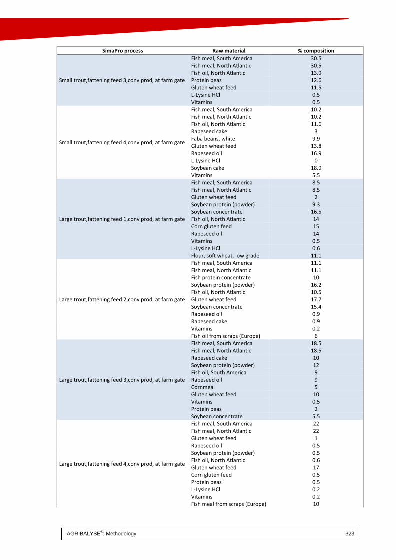
AGRIBALYSE®: Methodology 323
SimaPro process Raw material % composition
Small trout,fattening feed 3,conv prod, at farm gate
Fish meal, South America 30.5 Fish meal, North Atlantic 30.5 Fish oil, North Atlantic 13.9 Protein peas 12.6 Gluten wheat feed 11.5 L-Lysine HCl 0.5 Vitamins 0.5
Small trout,fattening feed 4,conv prod, at farm gate
Fish meal, South America 10.2 Fish meal, North Atlantic 10.2 Fish oil, North Atlantic 11.6 Rapeseed cake 3 Faba beans, white 9.9 Gluten wheat feed 13.8 Rapeseed oil 16.9 L-Lysine HCl 0 Soybean cake 18.9 Vitamins 5.5
Large trout,fattening feed 1,conv prod, at farm gate
Fish meal, South America 8.5 Fish meal, North Atlantic 8.5 Gluten wheat feed 2 Soybean protein (powder) 9.3 Soybean concentrate 16.5 Fish oil, North Atlantic 14 Corn gluten feed 15 Rapeseed oil 14 Vitamins 0.5 L-Lysine HCl 0.6 Flour, soft wheat, low grade 11.1
Large trout,fattening feed 2,conv prod, at farm gate
Fish meal, South America 11.1 Fish meal, North Atlantic 11.1 Fish protein concentrate 10 Soybean protein (powder) 16.2 Fish oil, North Atlantic 10.5 Gluten wheat feed 17.7 Soybean concentrate 15.4 Rapeseed oil 0.9 Rapeseed cake 0.9 Vitamins 0.2 Fish oil from scraps (Europe) 6
Large trout,fattening feed 3,conv prod, at farm gate
Fish meal, South America 18.5 Fish meal, North Atlantic 18.5 Rapeseed cake 10 Soybean protein (powder) 12 Fish oil, South America 9 Rapeseed oil 9 Cornmeal 5 Gluten wheat feed 10 Vitamins 0.5 Protein peas 2 Soybean concentrate 5.5
Large trout,fattening feed 4,conv prod, at farm gate
Fish meal, South America 22 Fish meal, North Atlantic 22 Gluten wheat feed 1 Rapeseed oil 0.5 Soybean protein (powder) 0.5 Fish oil, North Atlantic 0.6 Gluten wheat feed 17 Corn gluten feed 0.5 Protein peas 0.5 L-Lysine HCl 0.2 Vitamins 0.2 Fish meal from scraps (Europe) 10

AGRIBALYSE®: Methodology 324
SimaPro process Raw material % composition
Fish oil from scraps (Europe) 20 Soybean protein (powder) 5
Sea bass or sea bream,fattening feed 1,conv prod, at farm gate
Fish meal, South America 40.7 Fish meal, North Atlantic 20.4 Fish oil, North Atlantic 5.2 Soybean cake 8.5 Faba beans, white 24.7 Vitamins 0.5
Sea bass or sea bream,fattening feed 2,conv prod, at farm gate
Fish meal, South America 42 Fish meal from scraps (Europe) 16 Fish oil from scraps (Europe) 6.4 Corn gluten feed 6 Soybean cake 10 Rapeseed cake 11 Fish protein concentrate 8 Vitamins 0.5
3. Forage
The LCI data sets built for AGRIBALYSE (see Appendix G) were used as raw material for forage. As the LCI data sets for plant production included losses in the field, only the losses during storage and distribution of forage were taken into account for livestock production. Table 166 gives the loss rates used, depending on the type of forage and the type of use.
Table 166: Loss rates used to calculate the quantities of forage distributed, expressed as a percentage of the yield at farm gate (meaning field loss are implicitly accounted for). For pastures, losses comparing pasture yield/harvesting yield are accounted for.
Type of grass Loss at harvesting (in the
field)
Losses during storage (%
of yield at farm gate)
Losses on collection and
distribution (% of yield at
farm gate)
Total losses (% of yield at
farm gate)
Meadow without clover
Hay 15 2.3 5.75 8.05
Silage 5 13.26 10.2 23.46
Haylage 5 7.14 5.1 12.24
Meadow with clover
Hay 25 2.5 6.25 8.75
Silage 3 22.66 10.3 32.96
Haylage 7 10.7 5.35 16.05
Alfalfa
Hay 2.62 6.55 9.17
Silage 9.064 10.3 19.364
Haylage 3.159 5.85 9.009
Maize
Silage 13 1 14
Bibliography AGRIBALYSE 2016 Report of changes AGRIBALYSE v1.2=> AGRIBALYSE v1.3, available on
www.ademe.fr/agribalyse-en

AGRIBALYSE®: Methodology 325
Gac A., Cariolle M., Deltour L., Dollé J-B., Espagnol S., Flénet F., Guingand N., Lagadec S., Le Gall A., Lellahi A., Malaval C., Ponchant P. and Tailleur A.. 2010. GESTIM : Guide méthodologique pour l’estimation des impacts des activités agricoles sur l’effet de serre, document provisoire version 1.2, Juin 2010. CASDAR n°6147.
IFIP 2016 Projet Ecoalim, Optimisation environnementale des stratégies d’alimentation des animaux. http://www6.inra.fr/ecoalim/Le-projet
Nguyen T.T.H., Bouvarel I., Ponchant P and van der Werf H.M.G., 2012. Using environmental constraints to formulate low-impact poultry feeds. Journal of cleaner production, 28, 215-224.
.
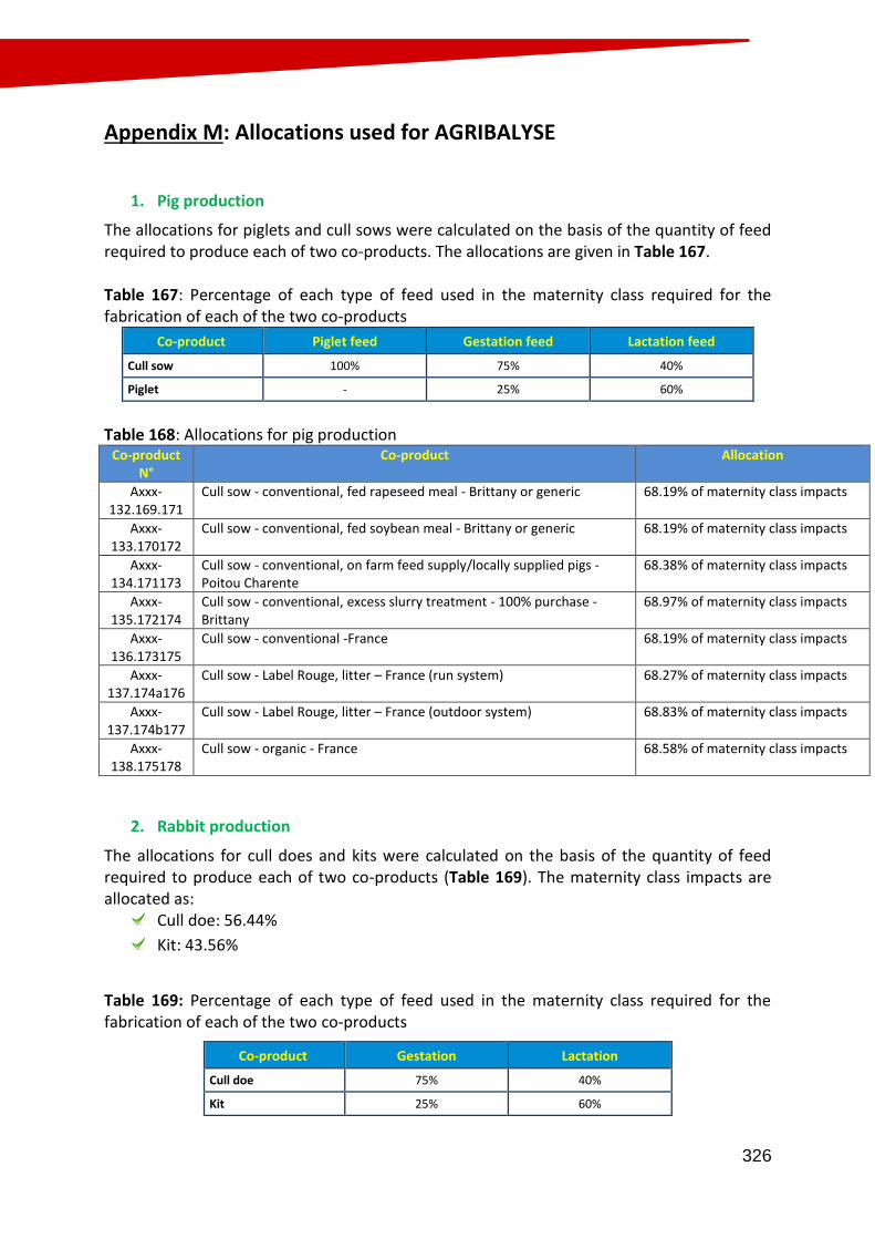
326
Appendix M: Allocations used for AGRIBALYSE
1. Pig production
The allocations for piglets and cull sows were calculated on the basis of the quantity of feed required to produce each of two co-products. The allocations are given in Table 167. Table 167: Percentage of each type of feed used in the maternity class required for the fabrication of each of the two co-products
Co-product Piglet feed Gestation feed Lactation feed
Cull sow 100% 75% 40%
Piglet - 25% 60%
Table 168: Allocations for pig production
Co-product N°
Co-product Allocation
Axxx-132.169.171
Cull sow - conventional, fed rapeseed meal - Brittany or generic 68.19% of maternity class impacts
Axxx-133.170172
Cull sow - conventional, fed soybean meal - Brittany or generic 68.19% of maternity class impacts
Axxx-134.171173
Cull sow - conventional, on farm feed supply/locally supplied pigs - Poitou Charente
68.38% of maternity class impacts
Axxx-135.172174
Cull sow - conventional, excess slurry treatment - 100% purchase - Brittany
68.97% of maternity class impacts
Axxx-136.173175
Cull sow - conventional -France 68.19% of maternity class impacts
Axxx-137.174a176
Cull sow - Label Rouge, litter – France (run system) 68.27% of maternity class impacts
Axxx-137.174b177
Cull sow - Label Rouge, litter – France (outdoor system) 68.83% of maternity class impacts
Axxx-138.175178
Cull sow - organic - France 68.58% of maternity class impacts
2. Rabbit production
The allocations for cull does and kits were calculated on the basis of the quantity of feed required to produce each of two co-products (Table 169). The maternity class impacts are allocated as:
Cull doe: 56.44%
Kit: 43.56%
Table 169: Percentage of each type of feed used in the maternity class required for the fabrication of each of the two co-products
Co-product Gestation Lactation
Cull doe 75% 40%
Kit 25% 60%

327
3. Cattle, sheep and goat production
The feed was allocated pro rata for the energy required for maintenance. The equations proposed in IPCC (2006b) were used. Net energy required by the animal for maintenance (cattle/sheep/goats)
𝑁𝐸𝑚 = 𝐶𝑓𝑖 × (𝑤𝑒𝑖𝑔ℎ𝑡)0.75 Where:
NEm is the net energy required by the animal for maintenance (MJ/day) Cfi is a coefficient which depends on the animal category (MJ/day/kg), see Table 170 Weight is the live weight of the animal (kg)
Table 170: Coefficients for calculating the net energy required for maintenance
Animal Coefficient
(MJ/day/kg)
Cattle- outside lactation period 0.322
Cattle- during lactation period 0.386
Cattle - bull 0.37
Sheep-lamb under one year 0.236
Sheep over one year 0.217
Net energy required for activity (cattle)
𝑁𝐸𝑎 = 𝐶𝑎 × 𝑁𝐸𝑚 Where:
NEa is the net energy required by the animal for activity (MJ/day) Ca is the coefficient for the animal’s feeding situation, see Table 171 ENm is the net energy required by the animal for maintenance (MJ/day)
Net energy required for activity (sheep/goats)
𝑁𝐸𝑎 = 𝐶𝑎 × (𝑤𝑒𝑖𝑔ℎ𝑡) Where:
NEa is the net energy required by the animal for activity (MJ/day) Ca is the coefficient for the animal’s feeding situation, see Table 171 Weight is the live weight of the animal (kg)

328
Table 171: Activity coefficient for the animal’s feeding situation
Animal Definition Ca
Cattle: Ca without size
Stall Animals are confined to a small area and expend very little energy to acquire feed
0
Pasture Animals are confined in areas with sufficient forage and expend an average amount of energy to acquire feed
0.17
Grazing large areas Animals graze in open range land or hilly terrain and expend significant energy to acquire feed
0.36
Sheep: Ca MJ/day/kg
Housed ewes enclosure Animals are confined due to pregnancy in the final quarter (50 days)
0.009
Grazing flat pasture Animals walk up to 1000 m per day and expend very little energy to acquire feed
0.0107
Grazing hilly pasture Animals walk up to 5000 m per day and expend significant energy to acquire feed
0.024
Housed fattening lambs Animals are housed for fattening 0.0067
Net energy required by the animal for growth (cattle)
𝑁𝐸𝑔 = 22.02 ∗ (𝐵𝑊
𝐶 ∗ 𝑀𝑊)
0.75
∗ 𝑊𝐺1.097
Where: NEg is the net energy required for growth (MJ/day) BW is the live body weight of the animal (kg) C is a coefficient of 0.8 for females, 1.0 for steers and 1.2 for bulls MW is the mature body weight of an adult animal (kg) WG is the daily weight gain (kg/day)
Net energy required by the animal for growth (sheep/goats)
𝑁𝐸𝑔 = 𝑊𝐺 × (𝑎 + 0.5𝑏 × (𝐵𝑊𝑖 + 𝐵𝑉𝑓))
𝐷𝑢𝑟𝑎𝑡𝑖𝑜𝑛 𝑜𝑓 𝑝𝑟𝑒𝑠𝑒𝑛𝑐𝑒
Where: NEg is the net energy required by the animal for growth (MJ/day) WG is the weight gain, PVf – PVi, (kg/day) BWi is the body weight on weaning (kg) BWf is the live weight at slaughter (kg) a, b are constants, see Table 172
Table 172: Coefficients for calculating the energy required for growth (sheep)
Category of animal a (MJ/kg) b (MJ/kg)
Rams 2.5 0.35
Castrated males 4.4 0.32
Ewes 2.1 0.45
Energy requirement during lactation (cattle)
𝑁𝐸𝑙 = 𝑚𝑖𝑙𝑘 × (1.47 + 0.40 × 𝑓𝑎𝑡) Where:
NEl is the net energy required for lactation (MJ/day) Milk is the quantity of milk produced (kg/day)

329
Fat is the fat content of the milk (% of weight) Energy requirement during lactation (sheep/goats)
𝐸𝑁𝑙 = 𝑚𝑖𝑙𝑘 × 𝐸𝑉𝑚𝑖𝑙𝑘 Where:
ENl is the net energy required for lactation (MJ/day) Milk is the quantity of milk produced (kg/day) EVmilk is the energy value to produce 1 kg of milk = 4.6 MJ/kg, equivalent to a milk fat
content of 7% in weight
Energy requirement for gestation (cattle/sheep/goats) 𝑁𝐸𝑔 = 𝐶𝑔𝑒𝑠𝑡𝑎𝑡𝑖𝑜𝑛 × 𝑁𝐸𝑠
Where: NEg is the net energy required for gestation (MJ/day) Cgestation is the gestation coefficient, see Table 173 NEs is the net energy required by the animal for maintenance (MJ/day)
Table 173: Coefficients for calculating the energy required for gestation
Category of animal Cgestation
Dairy cattle 0.10
Sheep
Single birth 0.077
Double birth (twins) 0.126
Triple birth or more (triplets) 0.150
Net energy required to produce wool (sheep)
𝑁𝐸𝑤𝑜𝑜𝑙 = (𝐸𝑉𝑤𝑜𝑜𝑙 × 𝑃𝑟𝑜𝑑𝑢𝑐𝑡𝑖𝑜𝑛𝑤𝑜𝑜𝑙
𝑝𝑒𝑟𝑖𝑜𝑑)
Where: NEwool is the net energy required to produce a year of wool (MJ/day) EVwool is the energy value of each kg of wool produced = 24 MJ/kg Productionwool is the average wool production per sheep over the period (kg/period)
Table 174 gives the allocations for cattle, sheep and goats.

330
Table 174: Allocations for cattle, sheep and goat production in AGRIBALYSE
LCI data set Ax class
Biophysical allocation co-products (%)
Other allocations
Milk Calf/lamb Wool Cull Ax
Co-product Key (%)
Type
Cow milk, conventional, lowland milk system, silage maize more than 30%, at
farm gate – Cull cow, conventional, lowland milk system, silage maize more than 30%, at farm gate atelier
Dairy cattle - Dairy cows in production
96.44 3.56
Dairy cattle - Calf (birth -"1 week")
Replacement calf
50.81 by
mass
Dairy cattle - Calf (birth -"1 week")
Beef calf 49.19 by
mass
Cow milk, conventional, lowland milk system, silage maize 10 to 30%, at farm
gate – Cull cow,
conventional, lowland milk system, silage maize 10 to 30%, at farm gate
Dairy cattle - Dairy cows in production
96.79 3.21
Dairy cattle - Calf (birth -"1 week")
Replacement calf
49.34 by
mass
Dairy cattle - Calf (birth -"1 week")
Beef calf 50.66 by
mass
Cow milk, conventional, lowland milk system, silage maize 5 to 10%, at farm gate- Cull cow, conventional, lowland milk system, silage maize 5 to 10%, at farm gate
Dairy cattle - Dairy cows in production
95.81 4.19
Dairy cattle - Calf (birth -"1 week")
Replacement calf
49.34 by
mass
Dairy cattle - Calf (birth -"1 week")
Beef calf 50.66 by
mass
Cow milk, organic, lowland milk system, silage maize 5 to 10%, at farm gate- Cull cow, organic, lowland milk system, silage maize 5 to 10%, at farm gate
Dairy cattle - Dairy cows in production
96.17 3.83
Dairy cattle - Calf (birth -"1 week")
Replacement calf
37.41 by
mass
Dairy cattle - Calf (birth -"1 week")
Beef calf 62.59 by
mass
Cow milk, conventional, highland milk system, grass
fed, at farm gate - Cull cow,
conventional, highland milk system, grass fed, at farm gate
Dairy cattle - Dairy cows in production
95.57 4.43
Dairy cattle - Calf (birth -"1 week")
Replacement calf
29.29 by
mass
Dairy cattle - Calf (birth -"1 week")
Beef calf 70.71 by
mass Sheep milk, conventional, Roquefort system, at farm gate-
Milk ewe - Lambs (0-weaning)
100
Milk ewe - Replacement gimmer 0-1 yr
1.36 98.64
Milk ewe - Ewe in production
88.71 9.28 2.01
Goat milk, conventional, intensive forage area, at farm gate
Milk goat - Goats in production
90.30 9.70
Lamb, conventional, indoor production system, at farm gate
Sheep for meat - Lambs 0-weaning
replacement 16.66 by
mass
Sheep for meat - Lambs 0-weaning
lamb for meat
18.34 by
mass
Sheep for meat - Lambs weaning-sale
100
Sheep for meat - Replacement
2.32 97.68

331
gimmers weaning-1yr
Sheep for meat - Replacement gimmers 1yr-2yrs
1.56 98.44
Sheep for meat - Sheep in production
98.80 1.42
4. Grassland / hay – grazed grass
As the LCI data sets for cut grass (hay, haylage, silage) cover mixed production systems (including grazing/cutting), there must be an allocation between the main product (cut grass) and the co-product (grazed grass). Mass allocation was used using generic values (yield of main product divided by the sum of the yields of the main product and the co-product, see column 3, Table 175). This was used for the inputs for the main product and the co-product. Harvesting (cutting, swathing, baling, transport, etc.) was allocated 100% to cut grass, because the work involved in harvesting is entirely for the cut grass (cf last column, Table 175). Table 175: Allocation for products and co-products for the 17 grass LCI data sets
LCI data set / crop Allocation Generic allocation
1
Grazed grass, permanent meadow, without clover, Auvergne, on field No, grazing only 100%
Baled grass, permanent meadow, without clover, Auvergne, at farm Yes, by mass
3.58/(2.41+3.58) = 60%
Grass silage, horizontal silo, permanent meadow, without clover, Auvergne, at farm Yes, by mass
3.58/(2.41+3.58) = 60%
Baled hay, permanent meadow, without clover, Auvergne, at farm Yes, by mass
4.18/(2.41+4.18) = 63%
Grazed grass, permanent meadow, without clover, Northwestern region, on field
No, grazing only
100%
Baled grass, permanent meadow, without clover, Northwestern region, at farm Yes, by mass
3.55/(4.92+3.55) = 42%
Baled hay, permanent meadow, without clover, Northwestern region, at farm Yes, by mass
4.22/(4.96+4.22) = 46%
Grazed grass, temporary meadow, without clover, Northwestern region, on field
No, grazing only
100%
Baled grass, temporary meadow, without clover, Northwestern region, at farm Yes, by mass
17.16/(17.88+17.16) = 49%
Baled hay, temporary meadow, without clover, Northwestern region, at farm Yes, by mass
20.88/(17.88+20.88) = 54%
Grazed grass, permanent meadow, with clover, Northwestern region, on field No, grazing only 100%
Baled grass, permanent meadow, with clover, Northwestern region, at farm Yes, by mass
3.29/(4.92+3.29) = 40%
Baled hay, permanent meadow, with clover, Northwestern region, at farm Yes, by mass
4.87/(4.92+4.87) = 50%
Grazed grass, temporary meadow, with clover, Northwestern region, on field No, grazing only 100%
Baled grass, temporary meadow, with clover, Northwestern region, at farm Yes, by mass
18.2/(19.68+18.2) = 48%
Grass silage, horizontal silo, temporary meadow, with clover, Northwestern region, at farm Yes, by mass
17.72/(17.88+17.72) = 50%
Baled hay, temporary meadow, with clover, Northwestern region, at farm Yes, by mass
4*5.87/(17.88+4*5.87) = 57%
1) Yield in t per hectare per assement period for LCI data set

332
5. Clementines
When the clementines have been harvested, they are graded by quality into two grades: clementines for export and clementines for local market. Economic allocation was used with the value defined by multiplying the quantities of the grades by their respective prices. The allocation for clementines for export was 86% (Table 176). Table 176: Allocation for product and co-product for the Clementine data set
Grade Yield Price Allocation
Clementines, export, SN – Average 330.6 t 3,000 Dirham/t 991,800/1,147,100= 86%
Clementines, local market 115.3 t 1,000 Dirham/t 115,300/1,147,100= 14%
6. Coffe
Economic allocation was done between coffee grain and pulp (in full production phase) : 4% of the impacts were allocated to pulp.
333
ADEME
The Agence de l'Environnement et de la Maîtrise
de l'Energie (ADEME) is a government
organization agency under the Ministry of
Ecology, Sustainable Development, Transport
and Housing, the Ministry of Higher Education
and Research and the Ministry of the Economy,
Finance and Industry. It is involved in the
implementation of government policies for the
environment, energy and sustainable
development.
ADEME provides environmental consultancy
services to help businesses, local authorities,
government authorities and the general public. It
also provides funding for projects, from research
to implementation, for waste management, soil
conservation, energy efficiency and renewable
energy, air quality and noise abatement.