AGRI-ENVIRONMENTAL INDICATOR...

AGRI-ENVIRONMENTAL INDICATOR PROJECT

Agriculture and Agri-Food Canada

REPORT NO. 6

INDICATOR OF RISK OF WATER

CONTAMINATION:

METHODOLOGICAL DEVELOPMENT

WORKING DRAFT

Prepared by:

Bruce MacDonald and Harry Spaling

March 1995

INDICATOR OF RISK OF WATER CONTAMINATION:

METHODOLOGICAL DEVELOPMENT

Prepared by:

Dr. K. Bruce MacDonald Ontario Land Resource Unit70 Fountain St Guelph, Ontario N1H 3N6

Tel: 519-766-9180 Fax: 519-766-9182

Dr. Harry SpalingDepartment of GeographyUniversity of GuelphGuelph, Ontario N1G 2W1

519-824-4120 (ex-2658)519-837-2940

with the assistance of:

R. Simard, Ste. Foy Research StB. Bowman, London Research CentreJ. Millette, CLBRRC. Chang, Lethbridge Research Station

Prepared for the Water Contamination Risk Indicator Team of the Agri-environmental Indicator Project

Draft of March 21, 1995

CONTENTSACKNOWLEDGEMENT i

1. INTRODUCTION 1

2. RISK-BASED APPROACHES 12.1 RISK ANALYSIS USING SPATIAL INDICATORS 1

2.1.1 Vulnerability Mapping 22.1.2 Risk Based on Buffer Strip Characterization 3

2.2 BUDGET APPROACHES TO RISK 32.3 RISK AS PROBABILITY OF EXCEEDENCE 42.4 RISK IN RATING INDICES/INDEXES 52.5 RISK AND EXPERT SYSTEMS 62.6 OVERALL ASSESSMENT 6

3. A PROPOSED METHODOLOGY FOR IROWC 63.1 CONSIDERATIONS FOR DEVELOPMENT OF THE METHODOLOGY 7

3.1.1 Hydrologic Considerations 73.1.2 Nutrient Considerations 83.1.3 Pesticide Considerations 83.1.4 Key Questions 9

3.2 ASSUMPTIONS 103.3 A PROPOSED BUDGET MODEL FOR IROWC 10

4. EXAMPLE APPLICATIONS OF THE PROPOSED METHODOLOGY 124.1 IROWC AS A RELATIVE MEASURE - BROAD LEVEL INTERPRETATION 12

4.1.1 Temporal variation 154.1.2 Composite indicator 16

4.2 IROWC AS AN ACTUAL MEASURE - ASSESSMENTS AT LOWER LEVELS (3-1) 164.2.1 Bamberg Creek Watershed 164.2.2 Extending the Research 184.2.3 IROWC at the level of the SLC polygon 24

5. POTENTIAL PILOT AREAS FOR DETAILED IMPLEMENTATION OF IROWC 24

6. ASSOCIATED RESEARCH AND COLLABORATION 25

REFERENCES 28

ACKNOWLEDGEMENT

The authors thank Dr. Fenghui Wang for his assistance with GIS analysis and mappreparation in the demonstration of the IROWC methodology.

1. INTRODUCTION

The purpose of this paper is to build on the hierarchical framework and concepts describedin a companion paper to develop a methodology for the Indicator of Risk of WaterContamination (IROWC) 1. The methodology is proposed as a preliminary model only. Itrequires further development and continued testing to authenticate its utility amonghierarchical levels, and at various temporal and spatial scales.

This discussion document describes the initial development and demonstration of IROWC,and suggests areas of further research, testing and implementation. The paper first brieflyreviews a number of risk-based approaches to the analysis and assessment of watercontamination by agriculture, based on previous research. It then proposes a methodologyfor IROWC using the budget approach. The proposed methodology is demonstrated utilizingpreliminary data and. finally, suggestions for detailed implementation are presented.

2. RISK-BASED APPROACHES

The potential of nitrates or pesticides to contaminate water is frequently determined byscreening or simulation models. Screening models assess and rank the leaching potentialof inputs. generally on the basis of chemical properties. Simulation models incorporatevarious physical. chemical and biological attributes of the input and site to predict theamount of a contaminant which is available for contamination. Both models are apparent inrisk-based approaches.

This section identifies and describes previous risk-based approaches to the analysis andassessment of nitrate and pesticide contamination of surface and ground water. It classifiesthe approaches into general categories and assesses their utility for IROWC using thedesirable characteristics of IROWC identified in the companion paper.

2.1 RISK ANALYSIS USING SPATIAL INDICATORS

Spatial indicators generally map spatial attributes of IROWC components (e.g., precipitation,soil leaching potential, crop type) to identify areas at risk of contamination. GIS is a commontool for analysis and display.

________________1 MacDonald, K.B. and H. Spaling. 1995. Indicator of Risk of Water Contamination: Concepts

and Principles. Working Paper. Draft of 21 March 1995, Agriculture and Agri-Food Canada,Ontario Land Resource Unit, Centre for Land and Biological Resources Research, Guelph,Ontario.

1

2.1.1 Vulnerability Mapping

Vulnerability maps identify and rate areas according to contamination potential. Vulnerabilityis based on the spatial association of attributes which affect contamination. Spatial analysisis usually integrated with a contaminant screening or modelling procedure.

A USDA study (Kellogg et al. 1992) developed vulnerability indexes for pesticide and nitratecontamination of shallow ground water. The Ground Water Vulnerability Index for Pesticides(GWVIP) is a function of soil-pesticide leaching, precipitation, and chemical use. The nitrateindex (GWVIN) is based on precipitation and excess nitrogen fertilizer (i.e., applied minuscrop uptake and removal). Index scores are grouped into relative categories of risk (high,moderate, low). Data are displayed at the national scale with county level resolution.

McRae (1991) also uses a vulnerability mapping procedure as part of a study to identifyareas at risk of ground water contamination in Canada. It is less comprehensive than theUSDA approach. The focus is on pesticide leaching potential, using only soil and landformcharacteristics derived from soil polygons on the Generalized Soil Landscape Maps(1:1,000,000). Areas vulnerable to pesticide leaching are characterized by sandy or sandyloam classes of soil texture, a slope gradient of 0-9%, and undulating, hummocky, level, orknoll and kettle classes of surface formation. McRae (1991) suggests improving theprocedure by including ground water recharge data.

The above studies generalize on the basis of soil type (e.g., sandy soils are equated withhigh leaching potential), but caution is needed since leaching may be higher in someinstances under other soils and certain management conditions (e.g., clay soils under ridgeor no-tillage where preferential flow is greater).

In another application, Khan and Liang (1989) use a GIS-based approach to construct mapsshowing the likelihood of pesticide contamination of ground water for Hawaii (1500 km2).A "contamination likelihood map" for various pesticides is based on an attenuation factor(AF) derived from the percent of applied chemical which leaches below the surface soillayers. A GIS is used to delineate the land area falling into different AF rating groups, andto calculate differences in contamination potential of the same pesticide for different crops.

These studies show that vulnerability mapping is capable of integrating IROWC componentsby determining their spatial association. The geographic scale and resolution of these studiessuggest that the procedure is most useful at levels 4-3 or higher. The analysis canincorporate a wide range of spatial attributes, although data requirements are extensive.The product (map) is easily communicated and interpreted. Applications focus on the riskof ground water contamination, but the procedure could be adapted for surface water.

2

2.1.2 Risk Based on Buffer Strip Characterization

This approach analyzes the width of an area adjacent to surface waters (riparian zone) whichacts as a protective strip to delay, assimilate or filter contaminants in runoff before theyenter a lotic system.

A buffer strip is a permanently vegetated area of land situated between the contaminantsource areas (i.e., agricultural fields) and the receiving waters. Buffer strips have thepotential to reduce contamination from diffuse sources through the retention of nitrogen,phosphorous and pesticides in runoff. Several reviews have assessed the effectiveness ofbuffer strips as a mechanism to reduce surface water contamination from agriculture(Muscutt et al. 1993. Osborne and Kovacic 1993, Phillips 1989).

Effectiveness (i.e., contaminant retention potential) is directly related to width of the bufferstrip, and the strip's environmental attributes and management characteristics. Width canbe determined by i) defining a constant distance (i.e., fixed setback from all surface waters).ii) establishing a minimum-variable distance (i.e., beyond a minimum, width variesdepending on environmental conditions and land use), or iii) using a variable distance basedon environmental and land use factors. Variable buffer widths have been calculated forstreams in a rural county of N. Carolina (Xiang 1993). This study incorporates a pollutantdetention time model into a GIS framework to analyze effectiveness of buffer strip widthsbased on soil hydrology, land cover and topography.

Buffer strips are most suitable as indicators of risk for surface water. Risk analysis andassessment could be based on deviation from an optimum buffer width. Variouscontaminants could be integrated into one indicator by identifying the contaminant with thewidest buffer requirement. Like vulnerability mapping, IROWC based on buffer strips isconducive to spatial presentation. which is easily communicated and interpreted. A need forcomprehensive data bases suggests that application is most appropriate at level 3, andperhaps 4. A significant shortcoming is that subsurface drainage (tile drains) is notaccounted for and could lead to an error in the calculation of risk for high rainfall areas (e.g.,eastern Canada).

2.2 BUDGET APPROACHES TO RISK

Budget approaches use input-output analyses to determine the amount of a plant nutrientor a pesticide which is in excess of crop requirements and may be available to contaminatewater.

Barry et al. (1993) use this approach to predict nitrogen balances for various crop rotationsin southwestern and western Ontario, and two farming systems (cash crop and dairy) inwestern Ontario. The quantity of surplus nitrogen is adjusted by an average ground waterrecharge rate to estimate the potential NO3-N concentration in shallow ground water(assumes an average ground water recharge of 160 mm yr-1 for southern Ontario based on

3

a proportion (51.8%) of the long term mean annual discharge of ten agriculturalwatersheds). For example, estimated nitrate concentrations in ground water under acorn-soybean-winter wheat rotation in southwestern Ontario was 8.5 mg NO3-N L-1 and 22.4mg NO3-N L-1 in western Ontario for the same cropping rotation, and 58.4 mg L-1 for a dairyfarm.

A major initiative to determine annual nutrient budgets for N, P and K is underway forseveral locations in the lower Fraser Valley of British Columbia (B. Zebarth, personalcommunication, 1995). An annual nutrient balance (applied surplus or deficit) is based ontype and number livestock, manure management, inorganic fertilizer applications, cropnutrient requirements, and atmospheric input. Estimates of soil release pathways includesurface and ground water. Data on inputs, pathways and outputs are differentiated on amonthly basis.

Budget approaches are also represented in calculations of mass balance to determine thedissipation of pesticides. For example, Frank et al. (1991a, 1991b) have calculated theproportion of applied atrazine, cyanazine and metolachlor which is dissipated by runoff,subsurface tile drainage, leaching to shallow ground water, and degradation in clay loamsoils of Ontario (field scale).

Risk is related to the quantity of a potential contaminant present in excess of a desirable ortolerable quantity. Risk is increased if a budget balance shows an excess amount. Unlikeindicators which focus on inputs or outputs (e.g., application rates per hectare, yield), abudget approach to IROWC considers the excess amount available for contamination2. Theabove studies by Barry et al. (1993) and Frank et al. (1991a, 1992b) apply a budgetapproach at the farm and field scales (levels 1 and 2), but it is potentially applicable athigher levels, as demonstrated in the nutrient budget calculations in British Columbia wherestudy areas represent an aggregation of farms. Also, crude nutrient budgets have beenestimated at the national level (see Table 9 in the concept paper). Factors which alter thebudget balance are readily incorporated (e.g., increasing use of conservation tillage).Notwithstanding the earlier reference to spatial indicators, a budget approach can beintegrated with spatial analysis to differentiate areas at risk of surface or ground watercontamination from nitrogen or pesticides.

2.3 RISK AS PROBABILITY OF EXCEEDENCE

This approach calculates an estimate of pesticide contamination in water, and expresses riskas a probability of exceeding an established or predefined water quality standard over adefined period of time.

_____________2 In areas with an annual deficit balance, unusual events may still contribute to water

contamination (e.g., high rainfall event (>50mm) on tile drained soils), but the relativecontribution is likely to be considerably less than that of a surplus balance.

4

Varshney et al. (1993) used this approach in a risk-based evaluation of ground watercontamination by atrazine, simazine and alachlor (southeast Iowa). The simulation modelRUSTIC provides estimates of concentrations of each herbicide within the aquifer (27-years).from which cumulative frequency distributions of herbicide concentrations at variouslocations are calculated. The potential risk (R) associated with each herbicide is defined as:

R = Pr (C>Cs)

where Pr = probability of exceedence, C = predicted daily pesticide concentration in groundwater (ppb), and Cs = maximum contaminant level (ppb) (EPA standards for eachherbicide). For example, simazine exceeded Cs 35% of the time.

This approach is attractive for IROWC because it explicitly incorporates a water qualitystandard, although there is no guidance for its selection. The use of a simulation model(RUSTIC) to estimate pesticide contamination is dependent on a long historical record. Forsituations of insufficient data, alternative probability distributions for estimating theprobability of exceedence of contaminant concentrations have been suggested by McBeanand Rovers (1992). Even if temporal limitations are overcome, the geographic applicationof this approach is likely limited to level 2, and maybe 3. Expressing risk as a probability ofexceeding a water quality standard is likely to be understood by non-technical people.

2.4 RISK IN RATING INDICES/INDEXES

Rating approaches rank contaminants according to their leaching potential. Ranking schemesfor nitrates are based mainly on soil properties, whereas those for pesticides consider thephysical and chemical properties of the material, as well as other soil, landscape andenvironmental characteristics. Land use and management are frequently held constant.

Khakural and Robert (1993) used LEACHM-N as a screening tool to develop soil NO leachingpotential (NLP) ratings from soil survey information and representative weather data.Seasonally accumulated values of leached NO3 (>1.5 m) for a normal precipitation year wereused as NLP indices. The ratings were added to the Soil Survey Information System (SSIS)to create NO3 leaching potential rating maps for three Minnesota counties.

McRae (1991) developed a pesticide rating scheme for Canada which ranked pesticidesbased on three factors: leaching potential, volume of use, and overall regulatory concern.Pesticides are ranked according to their leaching potential using Gustafson's technique(based on partition coefficient between organic carbon and water, and half-life of thepesticide in soil). Rankings by volume of use refer to kg/annum of active ingredient. Rankingaccording to overall regulatory concern reflects a pesticides status in the pesticidere-evaluation program. The scheme does not integrate the three rankings, but prompts theuser to consider each ranking in a sequential manner.

5

Other pesticide rating schemes also have been developed. For example, Warner (1985)proposed an environmental risk index which assigns a relative value to pesticides based ona tradeoff between its likelihood to contaminate (depending on persistence and mobility),and its toxicity. The index differentiates risk for surface and ground water, and is applied tovarious agricultural crops in Suffolk County, NY.

Rating approaches primarily focus on properties of contaminants and/or soils. For thisreason, their utility for IROWC is limited, unless integrated into, or accompanied by,approaches (e.g., spatial analysis) which consider other IROWC components (e.g., climate,land use, management).

2.5 RISK AND EXPERT SYSTEMS

Expert systems are computer models which help non-experts to find solutions to complexproblems. The models require not only quantitative data but also qualitative information inthe form of decision rules, interpretation and judgement.

Crowe and Mutch (1994) have developed an expert systems approach (EXPRES) to evaluatethe potential of a pesticide to contaminant ground water (see also Crowe 1994). Dependingon study objectives, available data and time constraints, EXPRES helps the user to select apesticide simulation model. prepare an input data set, carry out the assessment, andinterpret the results. The model provides a relative assessment of the potential of eachpesticide to contaminate ground water, including a quantitative prediction of the pesticidedistribution and migration rates (time and depth). The model is applied to a "typical" fieldof potato, irrigated sugar beet, and corn in PEI, Alberta and Ontario, respectively. (Themodel contains 22 agricultural regions in Canada).

Although EXPRES is designed primarily as a screening tool for decision making (e.g.,pesticide regulation), it has significant potential as an approach to IROWC. Presumably auser's objectives can be defined in terms of risk assessment. The main components ofIROWC are incorporated in the model. However, the model's field-specific focus is likely tolimit application to levels 1 and 2 although aggregation to level 3 and possibly 4 may bepossible for homogeneous conditions at these higher levels. The model requires detaileddata sets. While representative data sets are available with the model, ideally these shouldbe generated for each application.

2.6 OVERALL ASSESSMENT

The approaches reviewed here are relevant to the needs of IROWC and generally definesome potential methodological approaches. However, with the exception of the budgetingapproach, they fail to incorporate some characteristics of IROWC identified as desirable inthe concept paper. Specifically, most approaches provide a static assessment which doesnot incorporate specific farm management and production practices and does not readily

6

allow for temporal analysis.

3. A PROPOSED METHODOLOGY FOR IROWC

Risk of water contamination is based on a concentration of a potential contaminant in waterover time. Quite apart from the criteria used to define contamination, concentration dependson two variables:

1. the quantity of a potential contaminant, and2. the amount of water available to dilute it.

The amount of water available to dilute a potential contaminant is determined by waterpartitioning. At any site, total precipitation is partitioned into different forms. For example.during the growing season, a certain proportion of water is consumed by crops, and anotheris "lost" by evaporation from the soil surface. The remainder, or excess water above soilstorage capacity, moves off the site to recharge ground and surface water supplies.

3.1 CONSIDERATIONS FOR DEVELOPMENT OF THE METHODOLOGY

3.1.1 Hydrologic Considerations

In the proposed methodology, excess water plays a fundamental role in determining thelevel of risk of contamination. A water balance or budget approach can be used to determinethe quantity of excess water which is available to transport any residual amount of acontaminant. The basis for this approach is the terrestrial hydrological cycle. In this cycle,the main input (precipitation) is transformed through various processes (infiltration, plantuptake, runoff) into output (evapotranspiration).

Ideally, the water balance of an area is represented by the difference between precipitation(P) and actual evapotranspiration (AE). However, data for AE is frequently lacking. It ispossible to determine a crude water balance at any location based on annual or seasonalvalues of P and potential evapotranspiration (PE). When P exceeds PE, surplus moisture isassumed to exist and water accumulates in the soil until field capacity is reached. Anyfurther excess is available as surface water (i.e., runoff, subsurface tile flow), or groundwater recharge. When P<PE, a water deficit occurs, and there is no surplus moistureavailable.

A water balance approach can contribute to the proposed methodology in three ways. First.data on excess water can be distributed over time throughout the year. Seasonal or monthlyvalues of water surplus or deficit can be calculated, and analyzed against the temporaldistribution of excess nitrogen or pesticide residue. Second, the variation between years canbe assessed. Third, the water balance approach partitions output flow into surface (e.g.,runoff. seepage) and ground water (e.g., infiltration, deep percolation) components. Dataon the proportion of flow through each pathway is needed to analyze and assess the risk of

7

contamination according to destination.

Agriculture is directly dependent on the hydrological cycle (e.g., soil moisture for crops anddrinking water for livestock), but agriculture also alters the cycle, particularly the transfermechanisms and pathways of flow. For example, tillage practices affect infiltration rates,crop type and planting pattern influences runoff, and land drainage impacts percolation andlateral flow. These impacts become increasingly important at lower spatial and temporalscales. Thus, calculation of excess water at these scales needs to account for the effects ofland management on the water balance of an agricultural area.

While the pathways of the hydrologic cycle are reasonably well understood, goodquantitative estimates of the magnitude of flows in specific components are very difficult.

3.1.2 Nutrient Considerations

Nitrogen cycles in intensive, arable agriculture are generally characterized by the additionof nitrogen via fertilizer and/or animal manures, and the removal of nitrogen in theharvested crop and cover crops. Other inputs include atmospheric deposition and nitrogenfixation, while losses occur through leaching, denitrification and immobilization. Thesecomponents of the nitrogen cycle, and their proportionate amounts, are shown for wheatproduction in Figure 1.

Nitrogen in the form of fertilizer and manures often constitutes a large fraction of the totalnitrogen input. Generally, crops respond positively to increased fertilizer and manure inputs,but this response also increases nitrogen removed in the harvested material. Losses vialeaching are also usually higher with increasing nitrogen input. As fertilizer nitrogen isincreased, the efficiency of nitrogen use is decreased (i.e., percentage of total fertilizernitrogen taken up by the plant declines). Nitrogen use efficiencies for crops have beenbroadly estimated at 60-50% (e.g., Briggs and Courtney 1989, Juergens-Gschwind 1989).This means that a considerable quantity of nitrogen not taken up by plants is potentiallyavailable for leaching or other dissipation pathways of the nitrogen cycle.

3.1.3 Pesticide Considerations

An ideal approach to analyzing the risk of pesticide contamination first determines thequantity of a pesticide, and its chemical derivatives, in the soil, and then ascertains thesusceptibility of these chemicals to various transport and transformation processes (Mackay1992). Following application, a pesticide is partitioned into various phases (e.g., vapour insoil air, sorbed by organic matter, solution in soil water). Of particular concern is the amountpartitioned in mobile soil water, which represents the quantity potentially available forleaching or surface runoff. The proportion directed toward leaching can be relatively high forherbicides such as atrazine (Table 1). The risk of surface transport (in solution or attachedto eroding soil particles) is especially high if rainfall closely follows pesticide application.

8

Quantitative models of chemical fate in soil are available to estimate the amount of apesticide partitioned in soil water (e.g., PRZM, LEACHM). These models are generallysite-specific and applicable only at lower hierarchical levels (levels 3 - 1). Their datademands are extensive.

At higher levels (e.g., levels 5-3), information isavailable on pesticide inputs (e.g., recommendedapplication rates by crop, surveys of pesticide use),but understanding of and data on partitioning,transformation and transport are lacking. For thisreason, the relative indicator of risk of pesticidecontamination at level 5 considers pesticide inputdata only.

Table 1. Fate of Atrazine in Soil

Loss By:

reaction 31.4

leaching 68.0

evaporation to air 0.6

Source: data from Mackay (1991 )

3.1.4 Key Questions

Based on the methodological considerations discussed above, three questions forinvestigation can be posed:

1. Iis there sufficient excess water on average to move contaminants(vertically or laterally) to water sources (i.e., is there a risk?)

This question in reality deals not only with the amount of excess water, butalso the proximity of the rooting zone to water resources (surface or ground).It can be rephrased as "what is the travel time for potential watercontaminants to move to water resources?" It is only if the answer to thisquestion is yes or the travel time is short enough to be of concern that theremaining two questions are important. This is not to suggest that themovement of contaminants in water out of the active rooting zone is not ofconcern. It is simply to suggest that under these circumstances, it does notconstitute a risk of water contamination. This accumulation of a contaminantunder dry conditions over the long term resembles the condition of geologicnitrate described by Follett and Walker (1989).

2. What kinds of potential contaminants are present and in whatamounts?

At a detailed level, the answer to this question is quite complex and includessources such as atmospheric deposition, release from forms stored in soil andwetland components as well as the incremental inputs used in the course ofland husbandry. In this discussion, the indicator is focused on the specificpractices associated with agricultural land use. It may be thought of as apartial budgeting approach. In general then, the kinds and amounts of

9

potential contaminants are directly related to the kind of crop grown and thetype of agricultural system. From the standpoint of nutrients, there are threegeneral sources; namely, commercial fertilizer, decomposing crop residues andanimal manures. The amounts can be inferred from the current crop productionrecommendations, the amounts harvested in crop yields, and surveyinformation about the amounts produced or sold. For pesticides, the kinds andamounts can be inferred from the types of crops, current recommendedherbicide usage and surveys of actual use.

3. What is the quantity of water in excess of that used for cropproduction and evaporation? and, what is the fate of the excess water?

These are probably the most difficult and the most critical questions becausethey control the extent and direction of movement and the quantity of waterdetermines the dilution factor for all potential contaminants.

3.2 ASSUMPTIONS

At all but the lowest levels of the hierarchy, reasonable starting assumptions for agriculturalareas include:

1. an approximate balance between nutrient additions and removals within thelimits of nutrient use efficiency.

2. an indicator which estimates the impact of agricultural (anthropogenic)practices can be calculated using a partial budgeting approach which considersthose inputs and outputs directly influenced by management such as theapplication of fertilizers, manures and pesticides, and the removal of harvestedgrain and stover.

3. trends in pesticide use can be estimated from i) a knowledge of the cropsgrown and the recommended pesticides associated with their production, andii) the general level of pesticide usage (e.g., county level surveys).

4. for "average" conditions of soil, topography and drainage it is possible toestimate IROWC by crop (e.g., compared to non-crop or un-managedconditions).

5. at lower levels of the hierarchy it is possible to improve the IROWC estimatesby incorporating actual conditions of soil texture, topography, drainage etc andmore detailed climatic data.

6. it is necessary to estimate the extent to which "friendly" practices (e.g.,

10

conservation tillage, buffer strips) reduce the IROWC from that observed under"average" conditions.

3.3 A PROPOSED BUDGET MODEL FOR IROWC

This section describes a model for IROWC based on a budget approach. The model is viewedas a component of a broader methodological approach to IROWC, which will integrate thebudget approach with other tools (e.g., GIS) and approaches (e.g., spatial analysis of risk).The essential function of the model is to compare the flow-weighted mean concentration ofeach potential contaminant to an appropriate standard (e.g. drinking water). The risk ofwater contamination from non-crop and un-managed sources is acknowledged, but theapproach considers only the added risk of water contamination resulting from agriculturalactivities.

The Potential Contaminant Concentration (PCC) consists of two parts: i) determinationof the Potential Contaminant Present (PCP) in mg/ha, and ii) calculation of Excess Water(EW) in L/ha, representing the available quantity of surplus water. Thus:

PCC C = PCP (mg/ha) 3.3 (1)EW (L/ha)

c = contaminant type (e.g., nitrate, atrazine)PCP = f(climate, crop, input rates, soil, management, etc.)EW = f(precipitation, evaporation, crop moisture use (yield), soil).

At each level of the hierarchy, the differentiating characteristics and associated factors areincorporated into the determination of the amount or potential contaminant present (PCP).For example:

PCP5 = f(crop type, crop area, nitrogen in fertilizer and manure, nitrogen inharvested crop, herbicide class (e.g., triazine), annual climate normals).The calculated value is a relative indication where the non-crop or un-managed state is 0 and risk increases in proportion to nitrogen contentof the harvested crops, and level of pesticide use.

PCP3 = f(all information and constraints from higher levels plus crop rotations.soil texture, subsurface drainage, conservation practices, daily andmonthly climate, post-harvest precipitation, specific pesticide. etc.). Thecalculated value is the concentration in mg/ha for the specificcontaminant.

where 5 and 3 correspond to levels of the hierarchy. Excess water is determined byestimating the flows in the hydrological cycle in increasing detail at lower levels.

11

IROWC is characterized as the ratio of the average PCC to the concentration allowable tomaintain a desired standard (e.g., drinking water). Thus:

IROWC = PCCC (mg/L) 3.3 (2) Maximum Allowable concentration (mg/L),

IROWC composite = 'n

c=1 IROW c 3.3 (3)

Ideally, this calculation would be carried out for each (precipitation) event which constitutesa risk for water contamination. In practice, this will only be possible at the most detailedlevel of assessment. The hierarchial levels at which the indicator is required (see Table 1 inthe concept paper) determine the kinds of data available and the detail and precision whichcan be achieved.

In hierarchical fashion, we can start at the highest level and determine the constraints, andthen consider lower levels within these. For example, it is feasible to characterize IROWCat the ecoregion or ecodistrict level (levels 4-5). The proportion of the ecoregion orecodistrict occupied by various crops can be determined. At these levels, only a relativeindicator based on annual average conditions can be estimated. It is sensitive to changesin crop type, crop area, livestock density and monthly climate. It is not feasible toincorporate "friendly" practices because it is not possible to associate them with specificcrops (see Table 1 in the concept paper).

At lower levels (levels 1-3), the indicator will more nearly reflect actual conditions. It willrequire many more types of data in much greater detail to incorporate spatial variability insoil, topography and drainage; the degree of adoption of friendly practices and more specificdetails of climate. Temporal sensitivity is also better at lower levels allowing for calculationsof risk on a monthly or event basis. With the calculation of IROWC on the basis of soil units(e.g. SLC for level 3, detailed maps for level 2 and on-site soil characterization for level 1),it should also be possible to partition the risk of contamination into surface or subsurfacewater and possibly, tile drainage water. In addition, with movement from highest to lowestlevels, the probability of coincident occurrence (the certainty that the specific crop is grownon a known soil type using particular tillage practices, etc) increases, thereby enhancing thelevel of confidence for the estimate.

4. EXAMPLE APPLICATIONS OF THE PROPOSED METHODOLOGY

The following sections have been prepared at the request of the indicator team todemonstrate how the proposed methodology would characterize the risk of watercontamination. A full implementation of the proposed methodology is a substantialundertaking requiring consultation and input from many experts from across Canada andinternationally. In addition, it is to be expected that, as details of the methodology areworked out, there will be gaps in our knowledge and understanding which require original

12

research, and gaps in the available data which will require alternative data sources or datacollection activities. This could include coupling other agri-environmental indicators withIROWC, or direct incorporation of their data.

Consequently, THE SAMPLE IROWC CALCULATIONS SHOWN HERE ARE A DEMONSTRATIONOF THE METHODOLOGY ONLY. THEY HAVE NOT BEEN EXTENSIVELY CHECKED AND SHOULDNOT BE TREATED AS RELIABLE.

These examples do however provide a demonstration of the kinds of information which arerequired, the kinds of resolution which can be achieved and, very clearly, the levels of effortand detail which are needed to calculate something approaching ACTUAL indicators of riskof water contamination.

4.1 IROWC AS A RELATIVE MEASURE - BROAD LEVEL INTERPRETATION

Ideally, the proposed methodology would be implemented at all hierarchial levels. In reality,it is only possible to determine all parameters required at the lower levels. At the higherlevels only a relative IROWC rating is possible based on the principles outlined; namely, anestimate of the amount of potential contaminant(s) available, the amount of excess waterand the amount which could be accommodated within the standards of concern.

For the broad level assessments (levels 4 and 5), the IROWC is based on current land usepractices which give an indication of the level and kinds of inputs and climate records whichprovide a rough estimate of the quantity of water in excess of crop requirements. Theseresults could be presented at the level of ecozone, ecoregion or ecodistrict. The differencewould be in the degree of resolution of the classes and the extent to which specific landmanagement practices (such as conservation tillage. buffer strips. etc) could be considered.In addition, for the ecodistricts it would be possible to look at climate patterns for portionsof the year as well as the degree of variation between years.

For this demonstration example, the results are presented at the ecodistrict (ED) level. Thislevel and all larger spatial units are so large that the land use and management practicescannot be associated with specific soils, topography and drainage systems. Consequently.it is not possible to partition the IROWC between surface and ground water. Variations inspecific land management practices, or variation throughout the year or between years, canbe incorporated but are not illustrated in these examples.

The moisture conditions were estimated from climatic normals data for 1951-80. These datawere extracted from the Land Potential Data Base (Kirkwood et al., 1983) and associatedwith ecodistrict (ED) and SLC polygons by taking the largest area of overlap.

In keeping with the first question posed (section 3.1.4) the relative annual excess water(REW) or deficit was calculated from the annual precipitation (P) and the potential

13

evaporation (PE), using 1951-80 climatic normals data, as:

REW = Annual (P - PE) 4.1 (1)

The estimate of REW was determined for the prairie region and southern Ontario (Figure 2).In the prairies, all but the fringe areas are characterized by REW less than zero. While therewill be some movement of water to surface recharge areas at specific times of the year andalso some movement to ground water, at a broad level this movement is negligible. This isconsistent with the general landscape patterns of the great plains where most of thedrainage is internalized into prairie sloughs; the water tables are quite deep with littleconnection to surface recharge areas and there are few external drainage channels. Thisassessment is consistent with the observations of de Jong and Kachanoski (1987). Forfurther demonstrations of the proposed methodology, Southern Ontario is used as thesample region.

It is recognized that this approach to calculating annual excess water is not withoutproblems. Actual evapotranspiration (AE) is only a fraction of PE during most of the day inregions such as the prairies. This means that the above approach may underestimate annualexcess water. However, the approach is maintained because it is difficult to obtain data forAE at broad scales. A related problem is basing spatial screening on a single criterion (i.e.,REW). In the prairie region, it is possible to have both a small REW and a large potentialcontaminant concentration (PCC). The criterion of EW is maintained over concentrationbecause the fundamental matter of concern is water transport of the contaminant. Again,this does not imply that the steady accumulation of a contaminant under dry conditions andover the long term (e.g., geologic nitrate) is not important, but rather that its potential fortransport to surface or ground water is significantly reduced.

Ideally, PCC should incorporate variation in nutrient uptake efficiency and time of uptake foreach crop, as well as the temporal variability of excess water. Thus:

PCC = f(crop type, nutrient uptake efficiency, time of uptake) 4.1 (2) excess water f(time period) x crop area

Data constraints and the comprehensiveness of the analysis resulted in a simplified versionof this equation for the purposes of this demonstration. This analysis used mean annualvalues for P and PE (1951-1980 climatic normals) to estimate REW, and a mean nutrientuptake efficiency of 60% for all crops over the entire growing season.

Based on the above rationale, the following series of equations were used to estimate thebroad level IROWC for Southern Ontario:

14

RPCCN = 'ED Crop Area by crop x Nitrogen Harvested by crop 3 4.1 (3)

REW x total crop area

RPCCM = 'ED Nitrogen in Manure x 0.1 4.1 (4) REW x total crop area

RPCCH = 'ED Crop Area by crop x Average rate for herbicides by crop 4.1 (5)REW x total crop area

RPCC Ha = RPCCH x (P-PE) May + (P-PE) June x 0.5 + (P-PE) July x 0.25 4.1 (6)(Annual Precipitation - PE from 1951-80 climatic normals)

RPCC = relative potential contaminant concentration for nitrogen in the harvested crop (N),long-term nitrogen from manure (M), herbicide (H), and herbicide concentration adjustedfor the susceptible time (month) for transport (Ha). The herbicides atrazine and simazineare used for demonstration purposes.

IROWC (level 4.5) = (RPCCN + RPCCM)/10 + RPCCHa /0.01 4.1 (7)

The IROWC provides a measure of the relative amount by which the current standards areexceeded. The current drinking water standard for nitrogen is 10 mg/L and the standard foratrazine is 0.005 mg/L, and for simazine it is 0.01 mg/L. The latter standard is used tocalculate IROWC for herbicides.

Three additional considerations were included in the these equations:

1. Data on nitrogen use efficiency plotted against proportion of optimum yield(Sander et al. 1994) shows an efficiency of 60-40% for corn. Data from Europe(Juergens-Gschwind 1989) also suggests a nitrogen use efficiency of 60% andfurther indicates the other sink terms for the additional nitrogen (e.g.denitrification to GHG, soil biomass, transport off-site by water). This impliesthat the quantity available for other pathways is approximately equivalent tothe Nitrogen Harvested (equation 3). This efficiency is assumed for all crops.

______________3 The calculation determines the average quantity of nitrogen harvested per hectare of cropped

land in an ecodistrict based on the following levels of nitrogen in the harvested crop: Corn,grain and silage - 175 kg/ha; soybeans and white beans - 150 kg/ha; barley - 45 kg/ha;spring wheat - 55 kg/ha; winter wheat - 85 kg/ha; fall and spring rye and oats - 35 kg/ha:alfalfa and other tame hay - 200 kg/ha.

15

2. OMAF Publication 296 indicates the long-term value of manure. Generally, 50%of the total manure nitrogen (75% for poultry) applied in the spring is availablein the year of application. In the second year approximately 10% of theremaining nitrogen becomes available, 5% in the third year. For thiscalculation, the nitrogen during the year of application is included in theestimate based on harvested crop. For subsequent years a factor of 10% isused to account for the long-term value and also for the nitrogen lost frommanure applied (equation 4).

3. For herbicides, equation 6 is adjusted by the proportion of the excess moisturein May. June and July as these are the times the herbicide will be mostsusceptible to transport. These monthly figures are further weighed (l.0. 0.5and 0.25 respectively) to account for declining susceptibility to movementoff-site. After this time it is assumed to have been degraded by naturalprocesses. Atrazine and simazine are aggregated as triazines, and specificproperties of individual herbicides (e.g., solubility, half-life, partitioningcoefficient) are not considered at levels 4-5.

Key features demonstrated in the example application at the level 4-5 assessment aretrends and one option for calculating a composite indicator.

4.1.1 Temporal variation

Figure 3 shows the change between 1991 and 1981 in relative potential contaminantconcentration for nitrogen (based on levels harvested in the crop) for crop distribution asreported in the census of agriculture. These results are reported in units of mg/L or ppmwith the range going from a decrease of 5 or less to an increase of 5 or more. In generalthese results are quite encouraging for much of the province showing no change or a slightdecline. The greatest increase is indicated in the ecodistrict which occupies north Middlesexand the western portion of Huron Counties. In addition, there is some indication of anincrease in Eastern Ontario and Essex. Lambton counties and the fringe area. The mapillustrates that this kind of calculation can indicate some changes which are potentially of thesame order of magnitude as the drinking water standard.

4.1.2 Composite indicator

The ratio of the relative potential contaminant concentration (RPCC) to the maximumconcentration allowed by current standards provides an indication of risk. If all water qualitystandards have the same level of importance (or risk if exceeded) then it is possible toprovide a composite indication of risk by combining the risks for all separate potentialcontaminant components. This aspect is described by equation 7 and illustrated for Figures4a, 4b and 4c.

16

Figure 4a shows the relative IROWC associated with nitrogen from crop production and alsothe residual from previous manure applications. Figure 4b shows the relative IROWCassociated with triazine applications. Figure 4c shows the results of the combination of thesecomponent IROWC estimates.

4.2 IROWC AS AN ACTUAL MEASURE - ASSESSMENTS AT LOWER LEVELS (3-1)

As we move down the hierarchy, the resolution and accuracy of the IROWC should improve.In addition to the dominant factors affecting contamination at each higher level in thehierarchy, an assessment of risk at lower levels incorporates greater detail throughrefinement of parameters such as climate (e.g., monthly values of P-PE (or P-AE) to identifymonths when off-site movement is most likely), nutrient inputs (e.g., nitrogen uptakepattern of specific crops over the growing season to determine when surplus nitrogen ismost likely available). tillage practices (e.g., conventional, conservation, no-till) and theireffect on excess water and surplus nutrients, and processes such as subsurface tile drainageto further partition surface and ground water components.

An assessment of IROWC at lower levels incorporates these and other detailed parametersin order to estimate an actual concentration of a contaminant in water. In most cases, thiswill result in requirements for additional data and lead to increasingly complex analyses. Itwas not possible to develop a complete example demonstration of IROWC at lower levels.The following sections provide OUTLINES of how COMPONENTS of IROWC are assessed atlower levels. They also DEMONSTRATE the kinds of data which must be synthesized. Theresults are closer to ACTUAL BUT THEY ARE STILL RELATIVE.

Several attributes of IROWC are selected to demonstrate the type of parameters to beconsidered at lower levels. The geographic focus is on watersheds in south-western Ontariowhere flows and sediment yield have been monitored and, one small watershed in particular,Bamberg Creek.

4.2.1 Bamberg Creek Watershed

This watershed is a catchment located in Wilmot and Wellesley Townships in the RegionalMunicipality of Waterloo. Agriculture occupies about 81% of the watershed's land area in amix of farm types (e.g., cash crop, livestock, mixed farming). A recent study of thewatershed was undertaken to assess the state of the agricultural land base relative to itscontributions to non-point source pollution (Ecologistics Limited 1993). The study integratedavailable information on soils, land use and farm inputs (fertilizers, manures and pesticides)into a GIS framework to produce maps (1:50,000) of nutrient and pesticide loading, andground water contamination potential. The approach used approximates the preliminarysteps of a budget approach. Furthermore, data on soils, land use, and inputs of nitrogen andpesticides used in this study indicate the information base available for a level 3 assessment.

17

Nitrogen inputs were estimated using fertilizer nitrogen recommendations for the variousfield crops grown. These were converted to a unit area loading for each land use category(assuming different proportions of specific crops in various land use systems) and weightedby the proportion of each land use assumed to have received fertilizer. Estimates of nitrogenfrom manure were based on animal units (census data), manure production per animal unit,and average nitrogen concentration of manure. These values were adjusted to account foran estimated nitrogen loss of 50% during storage, handling and application. Arealproportions of manure application per land use system were assumed to determine unit arealoadings. The nitrogen values for fertilizer and manure, and total nitrogen, are shown byland use in Table 2. These data were used to produce a map of nitrogen loading (Figure 5).

Using 1986 census information, and data from the 1988 Ontario pesticide survey, the samebasic approach was used to estimate pesticide loadings by land use category. Pesticideswere not differentiated by type in this study. Crop groups were defined (row crops. smallgrains, hay and improved pasture) and assumptions made to estimate unit area pesticideloading for each group and distributed over the land use categories. Calculated pesticideloadings by land use category are shown in Table 2.

Finally, a map of soil transmissivity (i.e., ability of surficial soil (<1m) to transmit pollutants)was superimposed onto maps of nitrogen and pesticide loading to display the relativepotential for ground water contamination from these contaminants.

4.2.2 Extending the Research

The focus of the Bamberg Creek study was on characterizing the amounts of potentialcontaminants present. From the standpoint of an IROWC, there are additional data andinformation requirements. The analysis presented results on an annual basis with no attemptto deal with changing conditions throughout the year. There was no attempt to developcomplete budgets for nutrients or pesticides, and the complex and difficult task ofpartitioning water between surface, tile flow and ground water was not addressed. There areno easy ways of dealing with these concerns but the following sections indicate somepossible approaches and data sources which can be used.

1. Temporal Distribution of Surplus Nitrogen and Excess Water.

Nitrogen is present in the soil throughout the year and is normally added as fertilizer earlyin the growing season. The uptake of nitrogen by plants increases over the growing season.The pattern of nitrogen uptake can be analyzed in relation to surplus moisture distributionto determine the amount of mobile nitrogen in the soil profile.

Ontario data on plant uptake of nitrogen is available for some crops (M. Miller. personalcommunication). The quantity of nitrogen taken up by corn (grain and stover) is illustratedin Figure 6. Uptake commences after the first month of growth, increasing steadily between

18

Table 2. Nitrogen and Pesticide Loading by Land Use in Bamberg Creek Watershed.

Land useFertilizer N Manure N

Total NPesticides

(kg a.i. ha-1)- - - - kg N ha-1 - - - - -

Continuous crop 226 92 318 1.60Corn system 190 133 323 1.08Mixed system 165 162 327 0.73Grain system 102 39 141 0.40Hay system 126 342 468 0.33Pasture system 54 235 289 0.10Grazing system 0 169 169

source: data from Ecologistics Limited (1993)

32- 112 days after planting (DAP), and levelling off somewhat following Bilking (112 DAP).This pattern suggests that all of the applied nitrogen is surplus during the early stage ofplant growth. During subsequent growth stages, nitrogen uptake increases steadily (i.e., theamount of surplus nitrogen decreases). Over the entire growing season, total nitrogenuptake is approximately 200 kg ha-1.

The temporal distribution of nitrogen uptake can be compared to the seasonal or monthlydistribution of surplus moisture in order to estimate the quantity of nitrogen at risk ofleaching. An actual estimate can be derived using data on monthly or daily climatic normals(e.g., precipitation, potential evapotranspiration) for a representative climate station. Anexample for the Bamberg Creek watershed using climate data from Elora Research Stationis shown in Figure 6. There is a mean annual water surplus of 367 mm, but the distributionis such that a water deficit exists during the summer months (June - September). Thissuggests little risk of nitrogen movement during the growing season. Even 30 days afterplanting, when nitrogen uptake is nil (i.e., surplus nitrogen is high), the risk is low becausethe onset of water deficit coincides with planting of corn and fertilizer application (i.e.,mid-late May). Of course individual rainfall events may contribute to movement of surplusnitrogen throughout the growing season, as well as residual nitrogen in the soil atpost-harvest. This would require further detailed analyses using daily climate daily.

Crop uptake is an important, but incomplete, measure of recovery of applied nitrogen.Nitrogen is also partitioned in crop residue (surface stubble, roots) and in the soil as residualnitrogen. Like crop uptake, these also vary by crop type and rate of nitrogen application. Itwill be necessary to incorporate the changes in nutrients and water throughout the year toproduce a level 3 IROWC.

19

1. The use of Computer Simulation Models to Characterize the Dynamics ofspecific Pesticides in Soil Water.

Another way to incorporate the approach and results of Bamberg Creek watershed study intoan assessment of IROWC at level 3 is to determine the fate of specific pesticides usingmodels which estimate residual pesticide movement out of the root zone. The studyaggregates data on pesticide use but does not differentiate pesticides by type or rate ofapplication. Pesticides vary in their physical and chemical properties, and in their soil-waterinteractions. An analysis which considers various chemical transformations and partitioningof pesticide residue into differing sinks is best approached by use of a pesticide fate model(e.g., LEACHM, GLEAMS, PRZM). The spatial information on pesticide loading in BambergCreek watershed could be used to target specific sites (field, farm) for more detailed riskanalyses of pesticide movement.

In addition to site-specific applications, it is also possible to apply pesticide fate models atthe watershed scale. A recent study by de Jong et al. (1994) developed and applied amethodology to investigate migration of atrazine through the soil profiles (<90 cm) of theGrand River watershed. This watershed contains the Bamberg Creek catchment. The studydeveloped an integrated methodological framework consisting of 1) modified submodels ofLEACHM to describe soil water flow (LEACHW) and atrazine movement (LEACHP), 2)pedotransfer functions based on soil texture and organic carbon content, 3) geostatisticalanalyses to extend soil and climate data, and model output, from point to areal format, and4) GIS to produce maps of atrazine loading in the Grand River watershed (1:1,000,000).

Results of this study include model predictions of annual atrazine loading over time forseveral soils (Figure 7). Loadings vary by soil type, but tend to stabilize over time (after 5-8years) for all soils. Two of the soil types are found in the Bamberg Creek watershed (Huronclay, Fox sand). Atrazine movement in the Huron soil is characterized by an incrementalincrease in loading, stabilizing after year three. Presumably, atrazine applied to this soil isreadily degraded or its movement out of the soil profile is impeded (de Jong 1994). The Foxsand is distinguished by a relatively high atrazine loading, posing a greater risk of watercontamination.

Seasonal distribution of atrazine loading is not known since model simulations wereundertaken on an annual basis. Other factors (e.g., information on land use, crop rotations,and changes in water table depth) were excluded in the analysis, but the methodology hasconsiderable potential for analyzing the risk of pesticide contamination of ground water, andfor projecting the impact of changes in land use and pesticide management at the watershedscale.

3. Partition Excess Water into Surface Tile Drainage and Ground Water

A final suggestion for building on the Bamberg Creek watershed study to calculate a level3 IROWC assessment is to partition the excess water component into surface or groundwater. Ultimately, detailed analyses to quantify hydrologic pathways (e.g., runoff, base flow,

20

deep percolation) is best undertaken by hydrology models and use of long term data onclimate, stream flow, etc. However, it may be possible to use other data to approximate thewater partitioning. These alternative data sources include:

• estimates based on stream flow to quantify amount of water available to movecontaminants,

• analysis of land resource and management factors which influence moisturepartitioning, and

• output from the hydrology submodel of models already used to studysediment, nutrient or pesticide movement.

The Monitoring and Systems Branch, Ontario Region, Environment Canada, collects data onstream flow and sediment levels for a number of watersheds in south-western Ontario,including the watershed where Bamberg Creek is located. If we assume that the groundwater system is approaching equilibrium then stream flow will approximate the excess wateravailable. This measurement does not provide information on the portion of the water whichis surface runoff or the portion which has moved through the soil. Figure 8 shows thelocation of the 9 watersheds where stream flow data were available. Table 3 compares theexcess water as determined from climatic normals data to the 1972-1991 mean annualstream flow. Values of the stream flow estimate suggest that the actual quantity of excesswater is larger and more variable than the estimate based on climate. These results are tobe expected because:

• the climate data has been generalized over relatively large areas, and• actual evapotranspiration is always less than potential.

The partitioning of water between the soil surface and subsurface is determined by manyfactors. Rigorous estimates are quite difficult to make. There are, however, a number offactors of soil, landscape and management which can be used to provide a more qualitativeassessment. The soil polygons shown on Figure 8 partition the watersheds into differentareas depending on the land resource properties. Characteristics such as texture, slope andlandform have a strong influence on water pathways. Sandy textured soils are morepermeable and allow more flow through the soil and less runoff. Areas of greater slopesteepness and more dissected landform are conducive to higher proportions of runoff. Thesefactors are summarized in Table 4 for those soil polygons which are more than 50% withinwatershed boundaries.

Other factors which influence the water partitioning are the proximity to natural or artificialwatercourses. The stream network shown in Figure 8 was obtained from EnvironmentCanada. An analysis was done to determine the proportion of land adjacent to streams. Landwhich was within 200 meters of a stream was considered to be in close proximity. Therationale for the 200 meter buffer was that field boundaries tend to impede surface runoffand the traditional dimensions for fields in Ontario are 40 rods square or 200 x 200 meters.The stream proximity was calculated for each soil landscape polygon and, as shown in Table4, it varied substantially across the watershed area.

21

Table 3. Comparison of Annual P-PE and Annual Stream Flow in Selected Watersheds.

Watershed Station No. P-PE (mm) steam flow (mm)

1 02GB001 220 - 320 3842 02GE003 220 - 250 4223 02GG007 160 - 320 3234 02GC002 220 - 230 3625 02GC018 220 - 230 3916 02GCO26 220 - 230 4497 02GC021 220 - 230 5128 02GC007 220 - 230 3989 02GB007 220 - 230 312

Data Sources: 1) P-PE based on 1951-80 climatic normals (Kirkwood et al, 1983).2) Runoff based on 1972-91 observation of hydrologic stations, Monitoring

and System Branch, Environment Canada.

One of the more difficult aspects of water partitioning and, consequently, the destination ofpotential contaminants is flow through artificial subsurface drains. Water moving throughthis pathway will leach materials from within the soil profile but then is shunted to surfacewaters rather than contributing to base flow or ground water recharge. While the soiltaxonomy and natural drainage state provide some basic indications of presence or absenceof tile drains, maps of actual tile installations must be used to provide an realistic estimateof the proportion of drained land. Maps of tile drainage locations were available for portionsof the watersheds in Oxford, Middlesex and Elgin counties. Table 4 shows these estimateswhere data were available and illustrates the substantial degree of variation to be expected.

These factors illustrate the complexity of factors associated with the task of partitioningwater flows in the environment. Generally, models will be required to provide a realisticintegration. These models may be primarily for the hydrologic cycle or they may modelnutrient and pesticide flows in addition to water. For example, some hydrologic data shouldbe available for the Bamberg Creek watershed because the CREAMS model generallypartitions runoff and infiltration (using the SCS runoff curve number), and uses a waterbalance routing to account for storage in soil water, uptake by plants, and deep drainage.

Accurately partitioning excess water into surface and ground water components is achallenging hydrological task and an important area of further work.

22

Table 4. Some Land Resource and Management Factors which Affect the Partitioning ofExcess Water for Selected Watersheds of Southern Ontario (data compiled atSLC level).

Watershed

SLC poly #

Surface Texture

Slope(%)

LocalLandform

StreamProximity*

Prop. ofLand tiled

1 0078 Silt loam 1 - 3 Level 10.6 n/a0073 Clay loam 1- 3 Undulating 8.0 n/a0452 Clay loam 1 - 3 Undulating 1.3 n/a0066 Clay loam 1- 3 Level 5.6 n/a0153 Loam 1- 3 Undulating 4.8 n/a0077 Loam 4 - 9 Undulating 3.6 n/a0036 Loam 4 - 9 Rolling 7.4 15.8 0069 Loam 4 - 9 Undulating 6.6 n/a0070 Loam 10 - 15 Hummocky 5.4 n/a0471 Loamy sand 1- 3 Undulating 8.5 n/a0470 Loamy sand 1- 3 Undulating 7.7 n/a0049 Loamy sand 1- 3 Undulating 12.2 4.50067 Sandy loam 1 - 3 Undulating 5.1 n/a0068 Sandy loam 4 - 9 Rolling 5.3 n/a

2 0035 Silt loam 4 - 9 Undulating 5.0 47.7 0028 Silt loam 4 - 9 Rolling 12.0 51.2 0013 Silt loam 1- 3 Undulating 9.0 26.2 0038 Clay loam 1- 3 Undulating 8.9 36.0 0029 Loam 1- 3 Undulating 7.9 37.3 0034 Loam 4 - 9 Rolling 6.3 40.2

3 0026 Silt loam 1- 3 Undulating 8.7 38.1 0024 Clay loam 1- 3 Level 3.8 44.9 0020 Sand 1- 3 Undulating 6.8 4.90025 Sand 1- 3 Undulating 5.7 19.2

6 0424 Silty clay loam 4 - 9 Undulating 13.3 17.7 0423 Fine sand 1- 3 Undulating 6.6 8.3

7 0422 Loamy fine sand 1- 3 Undulating 11.4 n/a

9 0425 Clay loam 4 - 9 Ridged 0.0 15.5 0145 Loam 1-.3 Undulating 6.4 n/a0031 Loamy sand 1-3 Undulating 7.7 8.5

* proportion of land (%) within 200 meters (40 rods) of streams by SLC polygon

23

4.2.3 IROWC at the level of the SLC polygon

The discussions of data for a level 3 calculation of IROWC have dealt with watersheds, SLCpolygons as shown in Figure 8 and small catchment areas. As the size of the spatial unit getssmaller, it becomes increasingly difficult to assemble comprehensive consistent data overlarge areas. For example, it was possible to compile census of agriculture data on cropdistribution for SLC polygons. Other data such as climate, pesticide usage and farmingsystems cannot be directly related to SLC polygons. The climate station network is toosparse to be interpolated with precision. Pesticide usage is recorded on a substantially largerunits (counties) in classes. Farming systems can be compiled from census but requirementsfor confidentiality preclude this compilation at the SLC level.

Based on the crop distribution, the relative potential contaminant concentration for nitrogenbased on crop uptake was calculated for the watershed area. Figure 9 shows the results ofthis calculation for 1981 and 1991. This figure shows a substantial degree of change overthe time period and also shows the increasing complexity which results as the spatial unitsbecome smaller (i.e., approaching an actual IROWC).

5. POTENTIAL PILOT AREAS FOR DETAILED IMPLEMENTATION OF IROWC

The proposed methodology for IROWC must be implemented and tested using acceptedscientific principles and procedures. As it is implemented it will be important to review andrefine the data and scientific basis to ensure the best result. Before IROWC can be acceptedit must be validated. Testing must continue on an ongoing basis to ensure accuracy andrelevance.

At the general level (4-5), IROWC results will be validated by comparison to data from thelimited monitoring and experimental sites across Canada. As the IROWC methodology isdeveloped, refined and finalized it will be appropriate to select one research group, withsupport from a team of technical experts, to assemble the data and implement the level 4-5IROWC. Furthermore, the IROWC level 4-5 results will be compared to the IROWC calculatedat more detailed watershed and farm levels.

The lower level (2-3) IROWC sites become important locations for development of moreaccurate indicators and also as comparison sites for the general level 4-5 IROWC. Theirselection should be based on a variety of factors including:

• locations representative of the soils, land use and management andgeographical areas of agriculture in Canada,

• sites where data is available and collected on an ongoing basis to calculate themoisture balance and the budget of nutrients and chemicals in the environment,

• sites where past and ongoing monitoring activities are measuring theparameters necessary to test moisture and budgeting models.

24

• in light of current resource constraints, it will likely be necessary to incorporatethe detailed implementation of IROWC into closely related research projectswhich are already in progress.

The following is a list of some potential areas for detailed IROWC implementation:

1. the Lower Fraser River valley of B.C. where a major initiative is underway toestimate detailed nutrient budgets for specific agricultural locations. A focalpoint is the Abbotsford aquifer where a substantial project has been carried outto model ground water risks from intensive livestock-based agriculture.

2. the Lethbridge research station where projects relate to both dryland andirrigated agriculture and monitoring of nutrient and pesticide dynamics.

3. in Ontario, there are three small paired watersheds (Essex, Kettle and Kintore)where data collection and monitoring activities have been carried out for thepast 10 years. At the Essex site and the adjacent Woodslee Research substationdetailed hydrological measurements are being taken. At the Kintore site, thereis a large project currently under way to characterize water movement andassociated transport of chemicals.

4. in Eastern Canada there are a series of small watersheds which have beenextensively characterized and monitored in association with the InternationalHydrological decade. Since characterization of the hydrological cycle is criticalto the success of the IROWC methodology, it may be advantageous to usesome of these catchment areas.

In addition to the above, a survey is underway to collect information about a network ofCanadian watersheds (CANWANET) which have studies of relevance to IROWC (contactJacques Millette). Most of the studies are at level 2. See attached sample.

6. ASSOCIATED RESEARCH AND COLLABORATION

Implementation, testing and validation of the proposed IROWC methodology is bestundertaken by building on, and coordinating with, related research which is in progress orplanned. This section briefly identifies several associated research activities which shouldcontribute to further development and application of the IROWC methodology, and alsosuggests a general strategy of collaboration among research participants.

Research projects which have potential association with IROWC at the University of Guelphare listed below. This is a partial and incomplete list. Many other research projects are activeat other universities and research institutions across Canada, which should also beconsidered for their contribution to the methodological development of IROWC. The projects

25

listed below are selected and categorized relative to three broad components of IROWCwhich require further research and detailed data. The scale of implementation is also shown.

1. Estimation of surplus nutrients and pesticide residue, and their movement.Nitrogen balance for agricultural watersheds watershed

M. Goss, Department of Land Resource ScienceRetention of pesticides by Ontario soils plot

L.J. Evans, Department of Land Resource ScienceMovement of chemicals and bacteria off/out of the root zone field/watershed

D. Rudolph Centre for Ground Water Research (Waterloo) and G. Kachanoski, Department of Land Resource Science

(and other associated research)

2. Contamination partitioned by surface or ground water.Modelling the quality of surface and tile drainable water field

R. Rudra, School of EngineeringField techniques for measuring the hydraulic conductivity of soil field

D.E. Elrick, Department of Land Resource ScienceImpact of manure and fertilizer on nitrate contamination on groundwater field

E. Beauchamp and G, Kachanoski, Department ofLand Resource Science

Sustainable water use in southern Ontario regionalR. Kreutzwiser, Department of Geography


3. Effect of management practices on nutrient balance, pesticide fate and excess water.Effect of management on unsaturated transport properties of soil field

G. Kachanoski, Department of Land Resource ScienceControl of soil erosion and associated water pollution watershed

T. Dickenson. R. Rudra, School of EngineeringVariable rate application technology for N fertilizers (effect on leaching) field

G. Kachanoski. Department of Land Resource Science


A strategy of collaboration suggests that each research participant contribute its area ofexpertise to the development of IROWC. Such a strategy is briefly outlined below.

26

1. Research and development universities, agricultural research stations, centres ofof IROWC: expertise (e.g.. National Hydrology Research Institute)

2. Collaborative partnerships: federal-provincial agreements(e.g., Green Plan),stakeholder participation (participatory research),international consultation (e.g., OECD, Great LakesCommission)

3. Validation and calibration: water quality monitoring programs

27

REFERENCES

Barry, D., D. Goorahoo, and M. Goss. 1993. Estimation of nitrate concentrations in groundwater using a whole farm nitrogen budget. Journal of Environmental Quality 22:767-775.

Briggs, D. and F. Courtney. 1989. Agriculture and Environment: the Physical Geography ofTemperate Agricultural Systems. Longman Scientific and Technical, Harlow.

Crowe, A. and J. Mutch. 1994. An expert systems approach for assessing the potential forpesticide contamination of ground water. Ground Water 32:487-498.

Crowe, A. 1994. The application of expert systems to ground water contaminationprotection, assessment. and remediation. In U. Zoller (ed). Ground WaterContamination and Control. Marcel Dekker, New York, pp. 567-584.

de Jong, R., W.D. Reynolds, S.R. Vieira and R.S. Clements. 1994. Predicting PesticideMigration through Soils of the Great Lakes Basin. Centre for Land and BiologicalResources Research, CLBRR Contribution No. 94-70, Agriculture and Agri-FoodCanada, Ottawa.

de Jong, E. and R.G. Kachanoski. 1987. The role of grasslands in hydrology. In M.C. Healeyand R.R. Walace (eds.). Canadian Aquatic Resources. Can. Bulletin of Fisheries andAquatic Sciences 215. Dept of Fisheries and Oceans. Ottawa, Canada. pp 213-241.

Ecologistics Limited. 1993. Assessing the State of the Agricultural Resources - WilmotTownship and the Town of Whitchurch-Stouffville. Draft report prepared forAgriculture and AgriFood Canada (Guelph) by Ecologistics Limited, Waterloo.

Follett, R.F and D.J. Walker. 1989. Ground water quality concerns about nitrogen. In R.F.Follett (ed.). Nitrogen Management and Ground Water Protection. Elsevier,Amsterdam, pp. 1 -22.

Frank, R., 13. Clegg, and N. Patni. 1991a. Dissipation of atrazine on a clay loam soil,Ontario, Canada. 1986-90. Archives of Environmental Contamination and Toxicology21:41-50.

Frank, R., B. Clegg, and N. Patni. 1991b. Dissipation of cyanazine and metolachlor on a clayloam soil. Ontario. Canada, 1987-90. Archives of Environmental Contamination andToxicology 21:253-262.

Goss, M. D. Barry and D. Goorahoo. 1992. Sources and processes associated with nutrientcontamination of water resources. In M. Miller et al. (eds.). Agriculture and Water

28

Quality. Proceedings of an Interdisciplinary Symposium. Centre for Soil and WaterConservation, University of Guelph, Guelph, pp.35-44.

Juergens-Gschwind, S. 1989. Ground water nitrates in other developed countries (Europe)- relationships to land use patterns. In R.F. Follett (ed.). Nitrogen Management andGround Water Protection. Elsevier, Amsterdam, pp: 75-138.

Kellogg, R.L., M.S. Maizel and D.W. Goss. 1992. Agricultural chemical use and ground waterquality: Where are the potential problem areas? United States Department ofAgriculture. Washington, D.C.

Khakural, B. and P. Robert. 1993. Soil nitrate leaching potential indices: using a simulationmodel as a screening system. Journal of Environmental Quality 22:839-845.

Khan, M. and Liang. T. 1989. Mapping pesticide contamination potential. EnvironmentalManagement 13:233-242.

Kirkwood, V., J. Dumanski, A. Bootsma, R.B. Stewart, and R. Muma. 1983. The landpotential data base for Canada (revised 1989). LRRC Technical Bulletin 1983-4E.Research Branch, Agriculture Canada, Ottawa, Canada.

Mackay, D. 1992. A perspective on the fate of chemicals in soils. In M. Miller et al. (eds.).Agriculture and Water Quality. Proceedings of an Interdisciplinary Symposium. Centrefor Soil and Water Conservation, University of Guelph, Guelph, pp.1-11.

McBean, E. and F. Rovers. 1992. Estimation of the probability of exceedence of contaminantconcentrations. Ground Water Monitoring Review 12:115-119.

McRae, Blair. 1991. The characterization and identification of potentially leachable pesticidesand areas vulnerable to ground water contamination by pesticides in Canada. Issues.Planning and Priorities Division, Pesticides Directorate, Agriculture Canada.

Muscutt, A., G. Harris, S. Bailey, and D. Davies. 1993. Buffer zones to improve water qualitya review of their potential use in UK agriculture. Agriculture, Ecosystems andEnvironment 45:59-77.

Osborne, L. and D. Kovacic. 1993. Riparian vegetated buffer strips in water-qualityrestoration and stream management. Freshwater Biology 29:243-258.

Phillips, J. 1989. An evaluation of the factors determining the effectiveness of water qualitybuffer zones. Journal of Hydrology 107:133-145.

29

Sander, D.H., D.T. Walters and K.D. Frank. 1994. Nitrogen testing for optimummanagement. Journal of Soil and Water Conservation; Nutrient Management SpecialSupplement. 49:2, 46-52.

Varshney, P., U. Tim, and C. Anderson. 1993. Risk-based evaluation of ground watercontamination by agricultural pesticides. Ground Water 31:356-362.

Xiang, W. 1993. Application of a GIS-based stream buffer generation model toenvironmental policy evaluation. Environmental Management 17:817-827.

30

FIGURE CAPTIONS

Figure 1 Nitrogen Inputs and Outputs for Wheat Production (source: Juergens-Gschwind1989).

Figure 2 Climatic Moisture Index - P-PE in the Prairies and Southern Ontario.

Figure 3 IROWC - Change in Relative Potential Contaminant Concentration (RPCC) forNitrogen (1981- 1991) in Southern Ontario.

Figure 4a IROWC - Relative Risk of Contamination in Southern Ontario (Nitrogen - 1991).

Figure 4b IROWC - Relative Risk of Contamination in Southern Ontario (Triazine - 1993).

Figure 4c IROWC - Relative Risk of Contamination in Southern Ontario (Nitrogen andTriazine).

Figure 5 Nitrogen Loading in Bamberg Creek Watershed (source: Ecologistics Limited1993).

Figure 6 Nitrogen Uptake by Corn and Moisture Profile, Elora Research Station.

Figure 7 Predicted Annual Atrazine Loading (mg/m2) Over Time at 90 cm Depth for FourSoils in the Grand River Watershed (source: de Jong et al. 1994).

Figure 8 IROWC - Spatial Framework for Analysis at Broad Level in Selected Watershedsof Southern Ontario.

Figure 9 IROWC - Relative Potential Contaminant Concentration (RPCC) for Nitrogen inSelected Watersheds of Southern Ontario 1981 - 1991.

31

FIG. 1. Nitrogen Inputs and Outputs for Wheat Production.(source: Juergens-Gschwind 1989)

32

FIG. 3. IROWC - Change In Relative Potential Contaminant Concentration (RPCC) in Southern Ontario.

34

FIG. 4a. IROWC - Relative Risk Of Contamination In Southern Ontario.

Nitrogen (crop and residual manure) 1991

35

FIG. 4b. IROWC - Relative Risk Of Contamination In Southern Ontario.

Triazine 1993

36

FIG. 4c. IROWC - Relative Risk Of Contamination In Southern Ontario.

Nitrogen and Triazine

37

FIG. 5. Nitrogen Loading in Bamberg Creek Watershed (source: Ecologistics Limited 1993).

38

Fig. 6. Nitrogen Uptake by Corn and Moisture Profile - Elora Research Station.

Data Sources: 1) N uptake from M.H. Miller, Univ. of Guelph (personal communication), 2) Climatic data from Canadian Climatic Centre, Environment Canada.

39

FIG. 7. Predicted Annual Atrazine Loading (mg/m2) Over Time at 90 cm Depth for FourSoils in the Grand River Watershed (source: de Jong et al. 1994).

40

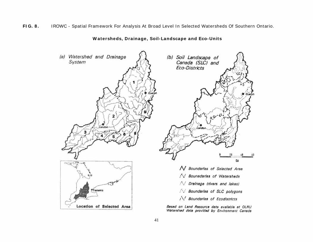
FIG. 8. IROWC - Spatial Framework For Analysis At Broad Level In Selected Watersheds Of Southern Ontario.

Watersheds, Drainage, Soil-Landscape and Eco-Units

41

FIG. 9. IROWC - Relative Potential Contaminant Concentration (RPCC) In Selected Watersheds Of Southern Ontario.

Nitrogen (crop) 1981 and 1991

42

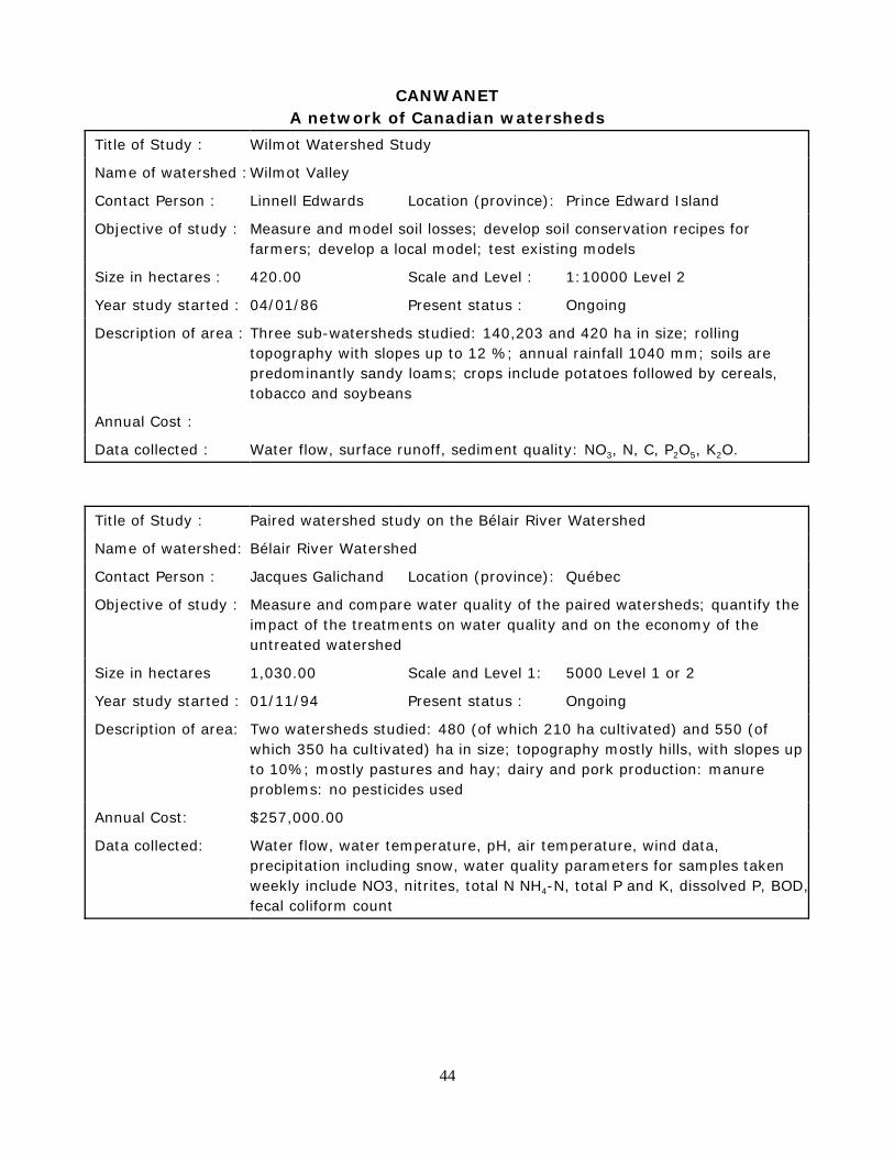
CANWANETA network of Canadian watersheds

Title of Study : Wilmot Watershed Study

Name of watershed :Wilmot Valley

Contact Person : Linnell Edwards Location (province): Prince Edward Island

Objective of study : Measure and model soil losses; develop soil conservation recipes forfarmers; develop a local model; test existing models

Size in hectares : 420.00 Scale and Level : 1:10000 Level 2

Year study started : 04/01/86 Present status : Ongoing

Description of area : Three sub-watersheds studied: 140,203 and 420 ha in size; rollingtopography with slopes up to 12 %; annual rainfall 1040 mm; soils arepredominantly sandy loams; crops include potatoes followed by cereals,tobacco and soybeans

Annual Cost :

Data collected : Water flow, surface runoff, sediment quality: NO3, N, C, P2O5, K2O.

Title of Study : Paired watershed study on the Bélair River Watershed

Name of watershed: Bélair River Watershed

Contact Person : Jacques Galichand Location (province): Québec

Objective of study : Measure and compare water quality of the paired watersheds; quantify theimpact of the treatments on water quality and on the economy of theuntreated watershed

Size in hectares 1,030.00 Scale and Level 1: 5000 Level 1 or 2


Description of area: Two watersheds studied: 480 (of which 210 ha cultivated) and 550 (ofwhich 350 ha cultivated) ha in size; topography mostly hills, with slopes upto 10%; mostly pastures and hay; dairy and pork production: manureproblems: no pesticides used

Annual Cost: $257,000.00

Data collected: Water flow, water temperature, pH, air temperature, wind data,precipitation including snow, water quality parameters for samples takenweekly include NO3, nitrites, total N NH4-N, total P and K, dissolved P, BOD,fecal coliform count

44

CANWANETA network of Canadian watersheds

Title of Study: Black Brook Experimental Watershed Study

Name of watershed: Black Brook Experimental Watershed

Contact Person : Lien Chow Location (province): New Brunswick

Objective of study : Provide quantitative information on surface and subsurface runoff; evaluatethe impact of various cropping systems environmental quality; validate andmodify existing models for N.B.

Size in hectares : 1,500.00 Scale and Level : Variable Levels 1 to 2


Description of area : Gently rolling topography with slopes varying from 1 to 9%; mostly potatocrop, rotation with grain, peas and hay; 65% of area agricultural land

Annual Cost :

Data collected : Water flow at 8 locations, surface runoff, climatic data, water quality data:sediment, N-NO3, P, K, Mg, Ca for all locations, pesticides at the outlet;

Title of Study : Predicting pesticide migration through soils of the Great Lakes Basin

Name of watershed: Grand River Watershed

Contact Person: Reinder De Jong Location (province) : Ontario

Objective of study: Develop methodology for predicting; conduct preliminary testing andevaluation of methodology

Size in hectares: 680,000.00 Scale and Level : 1:250000 Level 4

Year study started: 04/01/89 Present status : Ended in 1994

Description of area: Main crops are corn and soybeans: soil types range from sand to silty clay;annual rainfall 850-975 mm

Annual Cost : $100,000.00

Data collected: none

45

AGRI-ENVIRONMENTAL INDICATOR...

Documents

Transcript of AGRI-ENVIRONMENTAL INDICATOR...