juntal Ekonomi Malaysia 35 (2001) 37 - 60

Aggregate Import Demand and Expenditure Components in five ASEAN Countries: An Empirical Study

Mohammad Haji Alias Thck Cheong Tang Jamal Othman

A BSTRACT

This paper examines the 10llg run relationship between aggregate im­ports and expenditure components offive ASEAN countries using Johansen multivariate cointegration analysis. The ASEAN-5 countries considered are Malaysia, Indonesia, the Philippines, Singapore alld Thailand. AII­nual data for the period 1968-1998 are used lVith the exception of Singapore, with a shorter sample period, 1974-1998. The final demand expenditure variable is disaggregated into public and private consump­tion expenditure, investment expenditure alld exports. The use of a dis­aggregated demand variable, as opposed to the use of a single demand variable, is justified by the possibility that each final demand component may have different import contents. The approach employed in this study avoids the problem of aggregation bias. The results of Johansen s multi­variate test reveal that import demand is coillfegrated with its determi­nants for all ASEAN-5 cOllntries. Short-run variations in import demand found /0 be influenced by variations in relative prices and macro compo­nents oj final demand. Import demand is also found to be elastic lVith respect to relative prices for all ASEAN-5 countries except the Philip­pines. The findings provide a relevallt for policy implications.

INfRODUCTION

The main objective of this paper is to examine the long run relat ionship between import demand and the components of fmal expenditure, and relative prices for ASEAN-5 countries using Johansen multivariate cointegration analysis. The ASEAN-5 countries considered are Malaysia, Singapore, Thailand, Indonesia, and the Philippines. The components of

38 JI/mal Ekonomi Malaysia 35

final expenditures are final consumption expenditure, expenditure of in­vestment goods, and exports. An error correction model is proposed to model the short run response of imports to its determinants.

This study is justified by the following considerations. First, this study differs from most of earlier studies, which used a single demand variable in their specifications. Thi s approach implic itly assumes that the import content of each fi nal demand component is the same. If this as­sumption is not true, the lise of a single demand variable wi ll lead to aggregation bias. By disaggregating final demand we arc able to estimate the separate effects of each component on import demand.

Second, the findings wi ll be usefu l for evaluating 'he efficacy of ex­change rate policy to correct the trade balance deficits as experienced by most ASEAN countries in the years before the 1997 Asian Financial Crisis. The efficacy of exchange rate policy is based on whether the Marshall­Lerner condition is met or not. Relative prices do playa significant role in the determination of trade flow s, buttressing polic ies of devaluation as a way to correct trade imbalances (Reinhart 1995: 29 I). Trade theorists and analysts (for instance, Heien 1968) have long argued that for devaluation or depreciation to be effective in correcting trade imbalances, a value of the price elasticity of demand between - 0.5 and - 1.0 is necessary. This condition allows trade flows to respond to changes in relative prices in a significant and predicable manner (Reinhart 1995).

Third, the useaf cointegration methodology is more acceptable in the sense that, we are less open to the criticism of spurious regression should the variables involved in the import demand specification be non-station­ary in thei r levels.

The paper is structured as follows. The next section gives a review of selected recent studies on import demand. This is fo llowed by a section on model specification, and invest igation of the stationarity prope rt ies of the variables appearing in the import demand function. Section fo ur re­ports the empirical fi ndings. Section five reports the ECM analys is of short run behaviour of aggregate imports. The last section provides a summary and policy implications of the study.

REVIEW OFUTERATURE

This section reviews selected studies on import demand for the respective countries.

Aggregate Imporl Demand alld Expenditure Componen ts 39

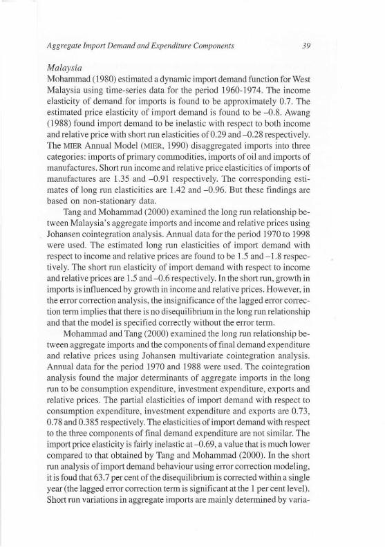
Malaysia Mohammad (1980) estimated a dynamic import demand function for West Malaysia using time-series data for the period 1960-1974. The income e lasticity of demand for imports is found to be approximately 0.7. The estimated price elastici ty of import demand is found 10 be -0.8. Awang (1988) found import demand to be inelastic with respect to both income and relative price with short run elasticities of 0.29 and -0.28 respectively. The MIER Annual Model (MtER, 1990) disaggregated imports into three categories: imports of primary commodities, impOlls of oil and imports of manufactures. Short nm income and relative price elasticities of imports of manufaclures are 1.35 and - 0.91 respecti vely. The corresponding esti­mates of long run elasticities are 1.42 and -0.96. But these findings are based on non-stationary data.

Tang and Mohammad (2000) examined the long run relationship be­tween Malaysia's aggregate imports and income and relative prices using Johansen cointegration analysis. Annual data forthe period 1970 to 1998 were used. The estimated long run elasticities of import demand with respect to income and relative prices are fou nd to be 1.5 and - 1.8 respec­tively. The short run elasticity of import demand with respect to income and relative prices are 1.5 and - 0.6 respectively. In the shall run, growth in imports is influenced by growth in income and relative prices. However, in the error correction analysis, the insignificance of the lagged error correc­tion tenn implies that there is no disequilibrium in the long run relationship and that the model is specified correctly without the error (elm.

Mohammad and Tang (2000) examined .the long run relalionship be­tween aggregate imports and the components affinal demand expenditure and relative prices using Johansen multivariate cointegration analysis. Annual dala for the period 1970 and 1988 were used . The cointegration analysis fou nd the major detenninants of aggregate imports in the long run to be consumption expenditure, investment expenditure, exports and relative prices. The partial elasticities of import demand with respect to consumption expenditure, investment expenditure and exports are 0.73, 0.78 and 0.385 respectively. The elasticities of import demand with respect to the three components of final demand expenditure are not similar. The import price elasticity is fairly inelastic at-O.69, a value that is much lower compared to that obtained by Tang and Mohammad (2000). In the short run analysis of import demand behaviour using error correction modeling, it is foud that 63.7 per cent of the disequilibrium is corrected within a single year (the lagged error correction term is significant at the 1 per cent level). Short run variations in aggregate imports are mainly determined by varia-

40 Jurnal Ekonomi Malaysia 35

lions in macro components of final demand expenditure viz. investment expenditure and exports, and relative prices.

Singapore Lim, Chow and Tsui (1996) applied demand systems specification to esti­mate Singapore's import demand function, and used the homogeneity restriction to yield efficient and consistent estimators in order to deal with simultaneity bias, measurement errors and omitted variables. This approach yielded better estimates than those obtained using the traditional log­linear model. The authors used augmented Dickey-Fullertest, but did not use the Johan sen and Juselius (1990) methodology probably because of the limited data available.

Aggregate imports are disaggregated into three categories: agricul­ture and mjning; fuels; and manufacturing. Annual data for the period 1975-1992 were used. The main results obtained in their study are as fol­lows. First, the respective demand in each sector is lypically most price elastic with respect to its sector price. Second, the income elasticities are positive for al l three sectors as expected a priori. A I per cent increase in income would lead to a 1.9 per cent increase in both agriculture and mining, and manufacturing imports, and 0.49 per cent increase in fuels imports.

Indonesia Reinhart (1995) specified and estimated an import demand function for Indonesia using annual data for the period 1970-1992. The esti mated long run elasticities of imports with respect to income and re lative price were 1.6 and - 0.9, respectively. The author using Johansen method found no cointegralion between imports and the other variables in the import func­tion. Senhadji ( 1998), based on annual data for the period 1960-1993 esti­mated the long run elasticities of income and price to be 0.98 and -1.56, respectively. However, the Phillips-Ouliaris residual test failed to reject the null of no cointegration. The corresponding short run income and price elasticities were found to be 0.36 and -0.62.

Thailand Bahmani-Oskooee (! 986) using quarterly data of 1973-1980 found that imports were inelastic, with estimated relative price and income elasticities - 0.308 and 0.946, respectively. Sinha ( 1997) used Johansen Multivariate procedure to estimate Thailand aggregate import demand function for the pcriod 1953- 1990, and found aggregate import demand to be price inelastic

Aggregate Import Demalid and Expenditure Componelits 41

(-D.77), and cross price inelastic (0.3) but highly income elastic (2. 15). Senhadji 's (1998) study found that the variables appearing in Thailand 's import demand model for 1960-1993, viz. real imports, ratio of imports de­Ilatorto GOP deflator and income (GOP minus exports) are not cointegrated. However, the estimated long run elasticities of income and prices were respectively, 1.67 and - lo43. The corresponding short- run elasticities were reported at 0.55 and -D.51. A recent study (Mah, 1999) reported that the estimated income and price elasticities of import demand were respec­tively, 0.74 (insignificant) and - lo53 forthe period 1963-92.

The Philippines Apostolkis (199 1) reported that the elasticities of income and relative price of Philippines's import demand were 0.67 and -2.73, respectively. A recent study by Senhadji (1998) estimated (OLS) that the long run income and prices elasticity of Philippines's import demand were at 2.25 and -2.73 respecti vely. Using annual data for the period 1960-93, they found that import demand was not cointegrated with its determinants (using Phillips­Ouliari s residual test). The short run elastici ties were 0.44 and -D.36 for income and prices, respectively.

In contrast, a study by Bahmani-Oskooee and Niroomand (1998) us­ing Johansen (1988) and Johansen and Jusel ius (1990) coin tegration meth­odology, fo und that there existed at least one cointegrating vector among the variables of import demand function (volume of imports, relative prices and domestic income) . The estimated long run elasticities of income and relative prices were 1.35 and - 1.01 , respec tively. Both stud ies found the Phil ippines import demand to be elastic with respect to income and rela­ti ve prices. The relati vely high-income elasticity suggests that import de­mand is strongly driven by economic growth. If imports are biased to­wards imports of consumption goods, ceteris paribus, the country may face balance of payments problems in the longer run.

THE MODEL AND DATA

The traditional specification of an import demand function relates the quantity of import demand to domestic real income and relative prices. The former is often proxied by an aggregate demand variable. The compo­si tion of expenditure is also argued to be important, if the various compo­nents of expenditure have different import contents (Giovannetti 1989; Thirlwall and Gibson 1992; Abbott and Seddighi 1996; and Mohammad &

42 Jumaf Ekollomi Malaysia 35

Tang 2000). If this were the case, the use of a single demand variable would lead to aggregation bias. Indeed, if the composition of demand changes, the aggregate import propensity would change even if the dis­aggregated marginal propensities are unchanged (Giovannetti 1989: 960).

In this study, final demand expenditure is disaggregated into con­sumption expenditure (private and public sectors), investment expendi­ture (public and private sectors) and exports.

The other important explanatory variable identified by economic theory is the price of imports relati ve to the domestic substitutes. The demand for imports is hypothesised to be inversely related to the relative prices term. An increase in relative prices leads to a fa ll in quantity of imports demanded, and vice versa. The small cou ntry assumption is in­voked here. Import supply elasticities are assumed to be infini te . Conse­quently, import prices may be treated as exogenous.

On the basis of the above assumptions, the long-run import demand function is specified as follows:

M, = f(FCE" EIG" EX" P,l (I)

where Fe E is final consumption expenditure. EIG is expenditure on invest­ment goods, EX is exports and P is relative price.

In this study we specified and estimated import-demand using the log-l inear fom] as fo llows:

Ln M, = IXD + IXI Ln FCE, + IX, Ln EIG, + IX] Ln EX, + IX, Ln P, + u, (2)

where ut is a random en'or assumed to satisfy the classical assumptions.

Ln stands for natural logarithms. From economic theory, the signs for the coefficients 0.

1, 0.

2 and 0.

3 are expected to be positi ve, and a~ to be

negative. The log-linear specification has been adopted by a number of studies

(Faini et al. 1992; Boyland et al. 1980; Goldstein & Khan 1985 and Beenstock et al. 1986). In all these studies, a single aggregate demand variable has been used as an explanatory variable. Exceptions are studies by Giovannetti (1989) and Mohammad and Tang (2000).

Annual data from 1968 to 1998 are used in this study, with the excep­tion of Singapore (1974-98) due to data availabi lity. All variables are in natural logarithmic fonn. Data sources and definitions are given in the Appendix I. We are not able to use quarterly data, as they are not available for a sufficiently long period for all the variables that appear in the import demand function, especially variables pertaining to the components of GD P. Quarterly figures may however be generated from annual data. Milham

Aggregate Import Demand and Expenditure Compmlellts 43

and Goh (1999) outlined some methods to generate quarterly figures from annual data. Ahmed and Tongzon (1998) used constructed real GOP quar­terly data for Malaysia supplied by Abeysinghe and Lee (1994), and for Indonesia, the Philippines and Thailand, quarterly data were generated from annual data obtained from International Financial Statistics using the Otani-Riechel's procedure used by the lMF. Their sample period is 1975 to 1993.

We are aware of the fact that the econometric techniques used in this paper are sensitive to the sample size or number of observations. When we use hard data collected by the relevant agencies, there is less criticism on the possibility of measurement errors. In this case we would have to generate quart.erly fi gures from annual data for a number of variables, in particular the expenditure components of final demand. But measurement errors may be more serious when data used are constmcted data. If mea­surement errors are correlated with regresors, use of OLS may lead to biased and inconsistent estimates. Another consideration when using quarterly data is that, seasonality effect needs to be addressed.

We can quote a number of studies on import demand functions lI sing a limited number of annual data. Doroodian, Koshal and Al-Muhanna (1994) used aggregate annual data for the period 1963-1990 (28 observa­tions). The authors used Dickey-Fuller (OF) and Augmented Dickey-Fuller (ADF) unit root tests and Johansen and Juselius multi variate trace and maximal eigenvalue cointegration tests. Rei nhart (1995) used annual data for the period 1968-1992 (25 observations). The authors used Johansen (1988, 1991) procedure in the context of a VAR model. Bahmani-Oskooee and Niroomand (1998) used annual data forthe period 1960-1 992 (33 ob­servations). They estimated import and export demand functions for about 30 countries. AOF tests and Johansen (1988) and Johansen and luselius (1991) cointegration analysis were carried out. A fmal example is Lim et al. (1996) who used annual data forthe period 1975- 1992 (18 observations). The authors used AOF test. The authors did not use the Johansen and lu seliu s (1990) me thodology probably becau se of the limited data avai lab le.

In carrying out a cointegration analysis , what matters is the length of the sample period and not so much the number of observations. As stated by Hakkio and Rush (1991), increasing the number of observations by using monrhly or quarterly data does not add any robustness to the re­sults in tests of cointegration. Sinha (1997) adopted this justification and employed cointegration approach (Johansen multivariate procedure) to

44 Jumal Ekonomi Malaysia j5

analyse aggegate import demand function for Thailand using annual timeseries data for the 1953- 1990 period.

We began by inyestigating the stationarity properties of the vari-ables appearing in the import demand function. According to phillips(1987), regressions involving levels of variables that are I(1) but notcointegated will yield spurious results. The implication of this is that,only cointegated yariables are to be used in regressions that involvelevels of the variables.

Both the AugmentedDickey Fuller (ADF) and the phillips-perron (pp)tests were conducted. The pp test was designed to be robust in the pres-ence of autocorrelation and heteroscedasticity. The regression equationfor the ADF test (Dickey and Fuller 1979) is given as follows.

k

LYt = q+bt +cyt_l+>di Lyt_i + et (3)

where A is the first difference operator, t refers to time fend. and I isadditional terms in the lagged differences for the Augmented Dickey-Fuller (ADF) test. e, is the regression error assumed to be stationary withzero mean and constant variance. The Phillips and Perron (1988) test isalso based on equation (3) but without the lagged differences. Both testswere caried out to reject the null hypothesis ofa unit root (c = 0 for ADF,andc=lforPP).

The datadefinitions and sources are given in Appendix l. The resultson the degree of integration of each series involved are repofied in Ap-pendix 2. The results show that all series are I(1) i.e. they become station-ary after first differencing.

Once the order ofintegration is established, and that the variables areall I(1), the search for a unique cointegrating vector using sets ofvariableswhich are integrated of the same ordeq is carried out. Johansen,s multi-variate cointegration tests are utilised for this purpose (Johansen 1988;Johansen & Juselius 1990). This approach can be used to establish thenumber of distinct cointegrating vectors. It does not haye the drawbacksof the Engle and Granger (1987) approach to cointegmtion (Abbott &Seddighi 1996: 1120). Having established that the variables entering theimport demand function are I(i), we then proceed to determine the laglength of the vAR, using the approach to ensure the residuals are whitenoise and have a normal disrribution.

Aggregate Import Demalld alld Expenditure Compollents 45

If the variables entering the import demand function are cointegrated, the ECM model is specified as follows:

11 II

M IlM I = bo + bli MIlM I-I + I, ~i MnFCE/-i + I, b:Ji MnElGt _ i i=O 1=0

II II n

+ I,b4i MnX ,_i ++ I,bSi Mn"'_i + I,b6i 6CU,_i (3) j=O j=O j=O

+ b7 EC t _ 1 + error _ term

where cu is capacity in the manufacturing sector for Malaysia and Singapore, where data are available . .6. stands for first difference operator. EC

t_

1 is the error correction term, the lagged residuals from the cointegrating

regression. This term is included if the variables appearing in the import demand function are cointegrated.

EMPIRICAL FINDINGS

This section reports the results of cointegralion analysis. The lohansen­Juselius (JJ) method of cointegration tests is based on the maximum likeli ­hood estimation of the VAR model. The trace statistics with the assump­tion of linear deterministic trend in the data (since there seems to be a linear trend in all the non-stationary series) are reported in Table 1.

TABLE 1. Trace test of Johansen cointegration method

Country: Eigenvalue Likelihood 5 Percent Adjusted 5 Hypothe-Ratio Critical Percent sized No.

Value Critical of CE(s) Value #

Malaysia (I) 0.71247 83.3578 68.52 81.68 None* Indonesia (2) 0.91444 151.0631 68.52 101.11 None* Thailand (I ) 0.82518 96.0575 68.52 81.68 None* Philippines (2) 0.88108 11 6.1867 68.52 10 1.1 1 None* Singapore ( I) 0.88562 11 7.3623 68.52 85.65 None*

Note: The 5 percent critical values, 68.52 for trace test are obtained from Osterwald­Lenum ( 1992, Table I). # The adjusted critical vaJues are computed with a scali ng factor proposed in Cheung and Lai ( 1993) to make finite-sample correct ion s. * denOles rejeclion of Ihe hypothesis al 5% signifi cance level based on adjusted critical values, and ( ) refers to optimal lag-length of VAR.

46 Jurnal Ekollomi Malaysia 35

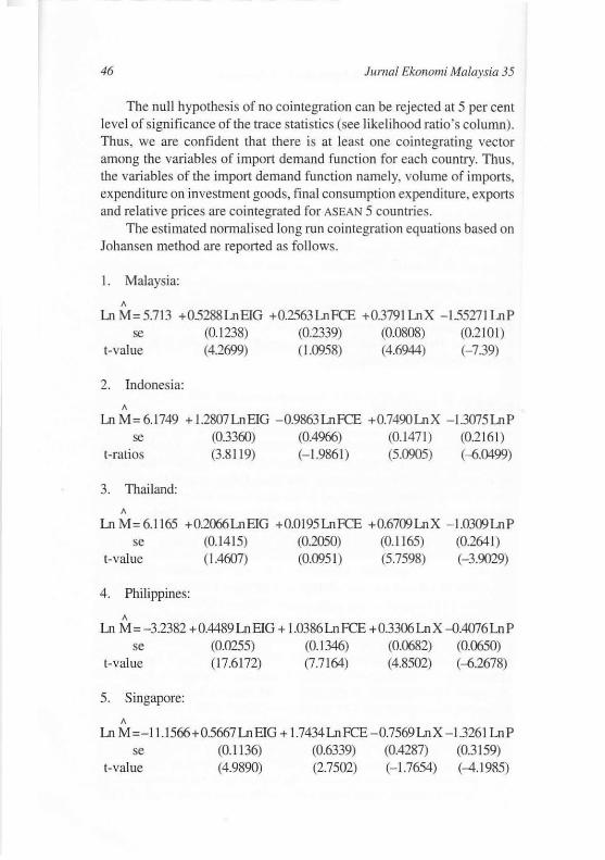
The null hypothesis of no cointegration can be rejected at 5 per cent level of significance of the trace statistics (see likelihood ratio's column). Thus, we are confident that there is at least one cointegrating vector among the variables of import demand function for each country. Thus, the variables of the import demand function namely, volume of imports, expenditure on investment goods, final consumption expenditure, exports and relative prices are cointegrated for ASEAN 5 countries.

The estimated normalised long run cointegration equations based on Johansen method are reported as follows.

I. Malaysia:

A

Ln M= 5.713 +0.5288LnEIG +0.2563LnFCE +0.3791 LnX -1.55271 LnP se (0. 1238) (0.2339) (0.0808) (0.2101)

t-value (4.2699) (1.0958) (4.6944) (-7.39)

2. Indonesia:

A

LnM=6.1749 +1.2807LnElG -0.9863LnFCE +0.7490LnX -1.3075LnP se (0.3360) (0.4966) (0. 1471) (0.2161)

t-ratios (3.8 119) (-1.9861) (5.0905) (-6.0499)

3. Thailand:

A

Ln M= 6.1165 +0.2066LnEIG +0.0195LnFCE +0.6709LnX - 1.0309LnP se (0.1415) (0.2050) (0.1165) (0.2641)

t-value (1.4607) (0.0951) (5.7598) (-3.9029)

4. Philippines:

A

Ln M= -3.2382 +0.4489LnEIG + 1.0386LnFCE +0.3306LnX -O.4076LnP se (0.0255) (0. 1346) (0.0682) (0.0650)

t-value (17.6172) (7.7164) (4.8502) (-6.2678)

5. Singapore:

A

Ln M=-11.I566+0.5667LnEIG + 1.7434LnFCE -0.7569LnX - 1.3261 LnP se (0. \136) (0.6339) (0.4287) (0.3 159)

t-value (4.9890) (2.7502) (-1.7654) (-4.1985)

Aggregate Import Demal/d Ql1d Expenditure Companel/ts 47

The results may be summarized as follows. First, all the estimated coeffi­cients have the correct signs, and most of them are significant at 5 per cent level of significance. with the exception of the Ln FeE variable for Malay­sia and Thailand. The export variable is also not significant at the 5 per cent level for Singapore. Second, the est imated coeffi cients for the final demand components for each country appear 10 be different. This sup­ports the approach of disaggregating the demand variable. Third, in all countries except the Philippines the estimated import price elasticity ex­ceeds unity. The estimate for Thailand is approximately unity.

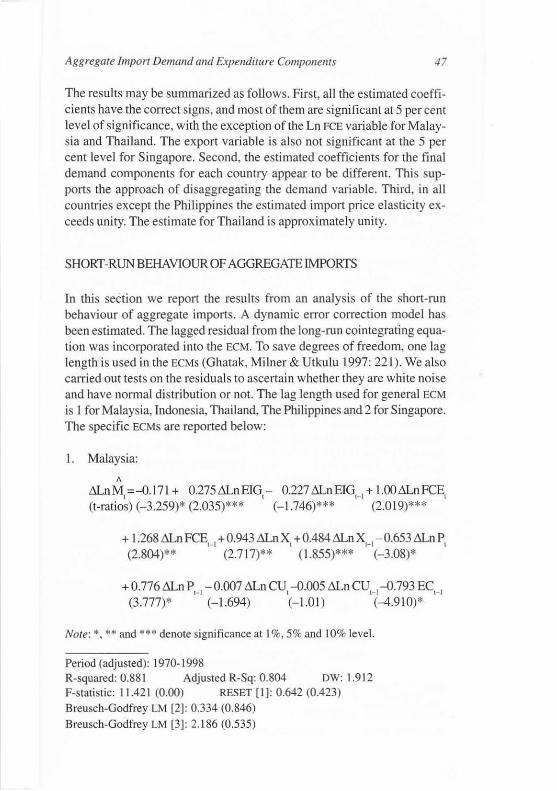
SHORT-RUN BEHAVIOUR OF AGGREGATE IMPORTS

In this section we report the results from an analysis of the short-run behaviour of aggregate imports. A dynamic error correction model has been estimated. The lagged res idual from the long-run coimegrating equa­tion was incorporated into the ECM. To save degrees of freedom, one lag length is used in the ECMS (Ghatak, Milner & Utkulu 1997: 221). We also camed out tests on the residuals to ascertain whether they are white noi se and have normal distribution or not. The lag length used for general ECM

is I for Malays ia, Indonesia, Thailand, The Philippines and 2 for Singapore. The specific ECMS are reported below:

I . Malaysia: ,

&nM,=-O.171+ 0.275&nEIG,- 0.227&nEIG,_,+ 1.00&nFCE, (t-ratios) (-3.259)* (2.035)*** (-1.746)*** (2.0 19)***

+ 1.268 &nFCE'_1 +0.943 &n X, + 0.484 &n X,_,-0.653&n P, (2.804)** (2.7 17)** ( 1.855)*** (-3.08)*

+ 0.776 &n P'_I - 0.007 &n CU, -0.005 &n CU'_I-O.793 EC,_, (3.777)* (-1.694) (-1.01) (-4.910)*

Note: *, ** and *** denote significance at 1 %,5% and 10% level.

Period (adjusted): 1970-1998 R-squared: 0.881 Adjusted R-Sq: 0.804 DW: 1.9 12 F-statistic: 11.42 t (0.00) RESET [1]: 0.642 (0.423) Breusch-Godfrey LM [2J: 0.334 (0.846) Breusch-Godfrey LM [3J: 2.186 (0.535)

Aggregate Import Demand and Expenditure Componellts 47

The results may be summarized as follows. First, all the estimated coeffi­cients have the correct signs, and most of them are significant at 5 percent level of significance. with the exception of the Ln FCE variable for Malay­sia and Thailand. The expon variable is also not significant at the 5 per cent level for Singapore. Second, the estimated coefficients for the final demand components for each country appear to be different. This sup­ports the approach of disaggregating the demand variable. Third, in all countries except the Phil ippines the estimated import price elasticity ex­ceeds unity. The estimate for Thailand is approximately unity.

SHORT-RUNBEHAV10UR OF AGGREGATE IMPORTS

In this section we repoll the results from an analysis of the shOll-run behaviour of aggregate imports. A dynamic error correction model has been estimated. The lagged residual from the long-run cointegrating equa­tion was incorporated into the ECM. To save degrees of freedom, one lag length is used in the ECMs (Ghatak, Milner & Utkulu 1997: 22 1). We also carried out tests on the residuals to ascertain whether they are white noise and have normal distribution or not. The lag length used for general ECM

is I for Malaysia, Indonesia, Thailand, The Philippines and 2 for Singapore. The specific ECMS are reported below:

I. Malaysia:

A

&nM,=-D. 17 1 + 0.275&nElG,- 0.227 &nEIGH

+ 1.00&nFCE, (t-ratios) (-3.259)* (2.035)*** (-1.746)*** (2.019)***

+ 1.268 &n FCE,_, +0.943 &nX, +0.484&nXH

- 0.653 &n P, (2.804)** (2.717)** (1.855)*** (-3.08)*

+ 0.776 &n P,_, - 0.007 &n CU, -D.005 &n CU,_,-D.793 EC,_, (3 .777)* (-1.694) (-1.01 ) (-4.910)*

Note: *, ** and *** denote significance at 1 %, 5% and 10% leve l.

Period (adjusted): 1970-1998 R-squared: 0.881 Adjusted R-Sq: 0.804 DW: 1.912 F-statistic: 11.421 (0.00) RESET [IJ: 0.642 (0.423) Breusch-Godfrey LM [2J: 0.334 (0.846) Breusch-Godfrey LM [3J: 2. 186 (0.535)

48 Jllmai Ekollomi Malaysia 35

Jarque-Bera: 1.593 (0.451 ) ARCH [ I J: 0.764 (0.382) White Heteroskedasticity: 24.853 (0.304) CUSUM and CUSUM of Squares show that the parameters are stable over the sample period. Note: ( ) refers to probability value.

2. Indonesia:

A

&n M, ~-D.049- 0.549&n M,_,+0.128 &n E[O, + 0.376&n EIOH

(t-ratio$)(- 1.038)(- 2.56)** (1.118) (2.416)**

+1.254&n FCE,_, + 0.500 &n X, +0.384&n X,_, -0.492 &n P, (2.63)** (2. 129)** (1.57) (-2.959)*

-D.745 &n P,_,- 0.093 EC,_, (-3.035)* (-1.041 )

Note : *. ** and *** denote significance at 1%, 5% and 10% leve l.

Period (adjusted): 1970-1998 R-squared: 0.751 Adjusted R-Sq: 0.634 DW: 2.086 F-statistic: 6.379 (0.00) RESET [I J: 1.919 (0. 166) Breusch-Godfrey LM [2J: 0.990 (0.609) Breusch-Godfrey LM [3J: 1.895 (0.594) Jarque-Bera: 1.979 (0.372 ) ARCH [ I J: 0.464 (0.496) White Heteroskedasticity: 18.663 (0.4 13) CUSUM and CUSUM of Squares show that the parameters are stable over the sample period. Note: ( ) refers to probability value.

3. Thailand:

A

&nM,~ -D.078 + 0.374&nE[O, + 16136LnFCE (t-ratios) (-3.437)* (3 .608)* (4.803)*

+ 0.290 &n X, + 0.246 &n P,_,- 0.4 17 EC,_, (1.960)*** (1.168) (-4.5 12)*

Note: *, ** and *** denote significance at 1 %, 5% and 10% level.

Period (adj usted): 1970-1998 R-squared: 0.889 Adjusted R-Sq: 0.864 DW: 2.084

Aggregate Import Denumd and Expenditure COmpOllellfS 49

F-statistic: 36.666 (0.00) RESET [I]: 1.278 (0.258) Breusch-Godfrey LM [2]: 1.908 (0.385) Breusch-Godfrey LM [3]: 3.357 (0.340) Jarque-Bera: 0.153 (0.926) ARCH [I]: 0.001 (0.973) White Heteroskedasticity: 17.107 (0.072) CUSUM and CUSUM of Squares show that the parameters are stable over the sample period. Note: ( ) refers to probability value.

4. The Philippines:

, &nM,=-O.031 + 00431 &nEIG, + Ul7 &nFCE, + 0.656 &n FCE,_, (t-rarios)(-1.245) (5.5 17)* (1.975)*** (\0410)

+ 0.314 &n X, - 0.192 &n P, + 0.154 &n P,_,-OA54 EC,_, (2.898)* (-10403) (1.155) (-3.00)*

Note : *, ** and *** denote significance at 1%,5% and 10% level.

Period (adjusted): 1970-1998 R-squared: 0.860 Adjusted R-Sq: 0.813 DW: 1.735 F-statistic: 18.355 (0.00) RESET [2]: 4.034 (0 .1 33) Breusch-Godfrey LM [2]: 1.194 (0.550) Breusch-Godfrey LM [3]: 8.1 74 (0.043) Breusch-Godfrey LM [4]: 9.621 (0.047) Jarque-Bera: 0.998 (0.607) ARCH [I]: 1.11(0.292) White Heteroskedasticity: 13.492 (0.488) CUSUM and CUSUM of Squares show thal the parameters are stable over the sample period. Note: ( ) refers to probability value.

5. Singapore: ,

&n M = 0.136 + 0.369 &n EIG -0.923 &n FCE t ! [-I

(t-ratios) (3.816)* (3.291)* (-1.637)

-O.330~Ln X,_,- 0.837 ~Ln P,-O.25I &nP'_2 (-2.34)** (-3.694)* (-1.517)

+0.007 &nCU, +O.O IO&nCU, + O.OO4&nCU,_, -O.401 EC,_, (4.900)* (5.383)* (1.851)*** (-30473)*

.lumal Ekonomi Mala'tsia 35

Noae x, x* and *** denote significance at 1%.57o aod' l01o level.

Period (adjusted): I 977- I 998

R-squared: 0.904 Adjusted R-Sq: 0.862 Dw: 1.828

F-statistic: 12.524 (0.00) REsEr []:0.008 (0.929)

Breusch-Godfrey LM [2]: 1.235 (0.539)

Breusch-Godfrey LM [3]: 1.504 (0.681)

Jarque-Bera: 0.354 (0.838 ) ARCH [2]:3.407 (0.182)

White Heteroskedasti ctty | 15.295 (0.642)

CUSUM and cusuM of Squares show that the pammeters arc stable over the

sample period.

Nore: ( ) refers to probability value.

The main results of the ECM analysis are as follows. First, on the basis

of vadous diagnostic tests, the ECMS fitted the data reasonably wellSecond, the significance of the lagged error correction terms in all counhy

EcMs at I per cent level, with the exception of Indonesia, indicates an

adjustment ofshortrun disequilibrium to a long run equilibrium. The size

of corrections of previous disequilibria, are estimated to be 79.3 per cent

(Malaysia), 41.7 per cent (Thailand), 45.4 per cent (Philippines), and 40.1

per cent (Singapore). The significance of the lagged error correction temsalso indicates weak-exogeneity of the independent variables, and Granger-

causality from independent variables to import demand. The insignifi-cance of the lagged error correction term in the case of Indonesia shows

that import demand is not cointergrated with its determinants (Kremers, et

al. 1992). However, we have a reservation of not using the result from a

single equation approach that checks for cointegration based on the t-

ratio of the error-corection term in a conditional error-correction model.

The singe equation approach (like EcM) is not appropdate in situations

where there are more than one cointegration vecto$. If there are more than

two variables in the model, there can be more than one cointegratinon

vector as in present study. A more poweful test to detect the number ofcointegrating vectors is system-based approach, like Johansen's (1988)

multivariate test. Since the Johansen test (Table 1) rejects the null ofnonecointegrating vector for Indonesia case, therefore, we can conclude that

the variables in Indonesian import demand function are cointegrated (at

least one cointegration vector).Third, short-run variations in import demand in the ASEAN-s coun-

tries are mainly determined by the variations in the macro components offinal demand expenditure and relative prices.

50 Jumaf Ekollomi Malaysia 35

Note: *. ** and *** denote significance at 1%,5% and 10% level.

Period (adjusted): 1977-1998 R-squared: 0.904 Adjusted R-Sq: 0.862 DW: 1.828 F-st.tistic: 12.524 (0.00) RESET [1]: 0.008 (0.929) Breusch-Godfrey LM [2]: 1.235 (0.539) Breusch-Godfrey LM [3]: 1.504 (0.681) Jarque-Bera: 0.354 (0.838) ARCH [2]: 3.407 (0. 182) White Heteroskedasticity: 15.295 (0.642) CUSUM and CUSVM of Squares show that the parameters are stable over the sample period. Note: () refers to probability value.

The main results of the ECM analysis are as follows. First, on the basis of various diagnostic tests, the ECMS fitted the data reasonably well. Second, the significance of the lagged error correction tenns in all country ECMS at 1 per cent level, with the exception of Indonesia, indicates an adjustment of short run disequilibrium to a long run equilibrium. The size of corrections of previous disequilibria, are estimated to be 79.3 per cent (Malaysia), 41.7 per cent (Thailand), 45.4 per cent (Philippines), and 40.1 per cent (Singapore). The significance of the lagged error correction terms also indicates weak-exogeneity of the independent variables, and Granger­causality from independent variables to import demand. The insignifi­cance of the lagged error correction term in the case of Indonesia shows that import demand is not cointergrated with its determinants (Kremers , et al. 1992). However, we have a reservation of not using the result from a s ingle equation approach that checks for cointegration based on the t ­

ratio of the error-correction term in a conditional error-correction model. The singe equation approach (like ECM) is not appropriate in situations where there are more than one coinregration vectors. If there are more than two variables in the model , there can be more than one cointegratinon vector as in present study. A more powerful test to detect the number of cointegrating vectors is system-based approach, like Johansen's (1988) multivariate test. Since the Johansen test (Table I) rejects the null of none cointegrating vector for Indonesia case, therefore, we can conclude that the variables in Indonesian import demand function are cointegrated (at least one cointegration vector).

Third, short-run variations in import demand in the ASEAN-5 coun­tries are main ly detennined by the variations in the macro components of final demand expenditure and relative prices.

Aggregate Import Demalld alld Expellditure Componell1s 51

SUMMARY

This study investigated the long-run relationship between quantity of import demand with it's detenninants viz. public and private consumption expenditure, investment expenditure and exports, and relative prices for fi ve ASEAN countries. The ASEAN countries chosen in this study are Ma­laysia, Thailand, Singapore, Indonesia and the Philippines. Di saggregar­ing demand variable into its components is justified in terms of the possi­bility of each expenditure component having different imp0rlcontents. By so doing, this study avoids the possibility of aggregation bias.

The main findings of this study may be summari sed as follows. The use of traditional specification of the import demand function in log-linear form, and disaggregating final demand variable, appear to be useful. The use of Johansen's multivariate cointegration analysis shows that import demand is cointegrated with its determinants for all ASEAN-5 countries. The ECM analysis shows that, short-run variations in import demand are influenced by variations in relative prices and macro components of final demand. An important frnding is that import demand is elastic with respect to relative prices. Only in the case of the Philippines that import demand is not price elastic.

The estimation of import demand functions is important for several reasons viz. structural analysis (to test trade theory), to forecast future imports and to evaluate the impact of government policies and exogenous shocks. In this study, the magnitudes of the price elasticity indicate that the Marshall-Lerner condition is easily met. This suggests that devalua­tion or a prolonged depreciation may be effective in correcting trade defi­cits. The 1997 Financial Crisis which affected all the ASEAN-S countries (to a lesser extent Singapore), which resulted in depreciation of the respective countries' currencies, have improved their export competitiveness, lead­ing to improvements in their trade balances and increased accumulation of international reserves. On the other hand, this finding also suggests that competition for export markets among the ASEAN-5 countries, especially among the countries which produce homogenous goods such as resource­based products (palm oil, rubber, wood-based) will be stiffer, given pro­longed depreciation. This is more so in the case of Malaysia where the Ringgit is still tied with the us dollar at a fixed level. A stronger dollar inevitably negates the competitiveness of Malaysian exportables relative to her counterparts. A more thorough investigation is needed in order to understand better the Malaysian export competitiveness and economy-

52 JUrlwl Ekollomi Malaysia 35

wide repercussion should the current exchange rate policy and peg level are to be sustained in the longer run.

The findings from this study may be connected to that of Ahmed and Tongzon's (1998) study on economic linkages among the five founding members of ASEAN viz. Malaysia, Indonesia, Thailand, Singapore, and the Philippines. Usi ng Vector Autoregression, variance decomposit ion and impulse response analyses applied to quarterly real GDP data forthe 1975-93 period, the authors found that Indonesia is the dominant economy that influences the other ASEAN economies. Spillover effects from the other ASEAN economies on Indonesia were found to be not significant. The Singapore and Malaysian economies arc most closely linked because of geographical closeness, economic and cultural factors. In our study, the estimated long nm elasticity ofIndonesian import demand with respect to expenditure on investment goods and exports are 1.28 and 0.75 respec­tively. An implication of these results is that growth in the final demand components would lead to growth in Indonesian imports in the long run. Pmt of the imports would be from other ASEAN member countries. Similarly growth in Malaysian import demand would be beneficial to Singapore's economy.

Aggregate Import Demalld and Expenditure Comporlems 53

APPENDIX I

DEFINITION OF VAR IABLES AND DATA SOURCES

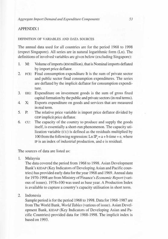
The annual data used for all countries are for the period 1968 to 1998 (expect Singapore). All series are in natural logarithmic form (Ln). The definitions of involved variables are given below (excluding Singapore):

I. M: Volume of imports (RM million), that is Nominal imports deflated by import price deflator.

2. FeE: Final consumption expenditure It is the sum of private sector and public sector final consumption expenditures. The series are deflated by the implicit deflator for consumption expendi­ture.

3. BIG: Expenditure on investment goods is the sum of gross fixed capital fonnation by the public and private sectors (in realtenns).

4. X: Exports expenditure on goods and services that are measured in real term.

5. P: The relative price variable is import price deflator divided by GDP implicit price deflator.

6. CU: The capacity of the country to produce and supply the goods itself, is essentially a short-run phenomenon. The capacity uti­lization variable (cu) is defined as the residuals multiplied by 100 from the fo llowing regression: Ln !P, = a + b time + e, where IP is an index of industrial production, and e is residual.

The sources of data are listed as:

I. Malaysia The data covered the period from 1968 to 1998. Asian Development Bank's KIDAP (Key Indicators ofDevelop;ng Asian and Pacific coun­tries) has provided early data for the year 1968 and 1969. Annual data for 1970-1998 are from Ministry of Finance's Economic Report (vari­ous of issues). 1978= I 00 was used as base year. A Production Index is avai lable to capture a country's capacity utilisation in short term.

2. Indonesia Sample period is forthe period 1968 to 1998. Data for 1968-1987 are from The World Bank, World Tables (various of issue). Asian Devel­opment Bank, KIDAP (Key Indicators of Developing Asian and Pa­cific Countries) provided data for 1988-1998. The implicit index is based on 1993.

54 Jumaf Ekollomi Malaysia 35

3. Thai land The sample period is 1968-1998. The generated base year is 1988. World Tables provided the annual data from 1968 10 1988 and KIDAP

for the following data source.

4. Philippines The data sources are World Tables (for annual data 1968-74) and KIDAP (1975-1998). All implicit index deflators with base year 1985=100.

5. Singapore International Financial Statistics Yearbook ( 1999) has provided a set of available annual data from 1974 to 1998. The base year is 1995. In contrast (Q other countries, the volume of imports and exports (measured by index) are collected from line 73 and 72 respectively. Imparl price index is from line 76.x. The two components of final expenditures, final consumption expenditure (sum of government and private seclOr) are deflated by GDP deflator (1995= I (0). The manufac­turing production index allows us to include capital utilisation in short run analysis.

Aggregate Import Demand and Expenditure Components 55

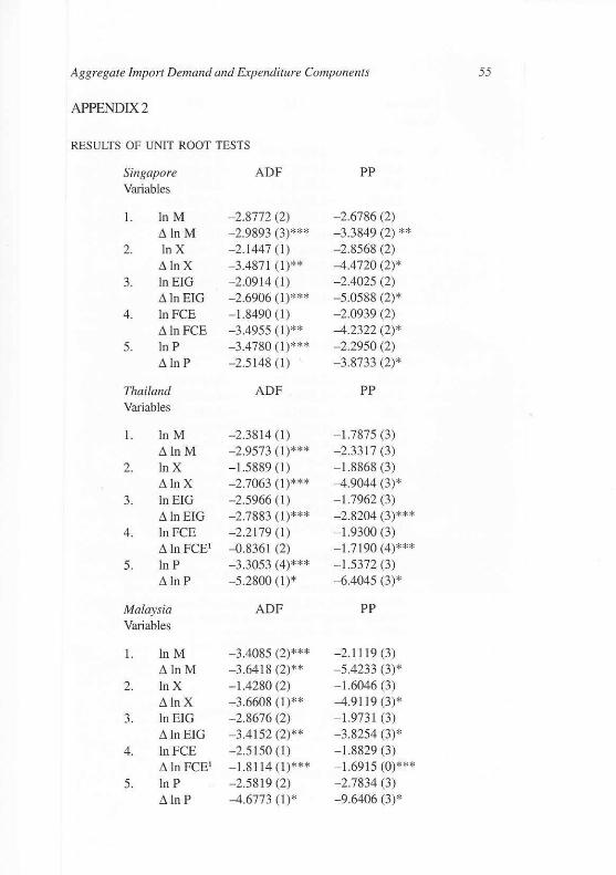
APPENDIX 2

RESULTS OF UNIT ROOT TESTS

Singapore ADF PP Variables

I. In M - 2.8772 (2) - 2.6786 (2) 8. InM -2.9893 (3)*** -3.3849 (2) **

2. In X - 2.1447 ( I) -2.8568 (2) 8.InX -3.487 1 (1)** -4.4720 (2)*

3. InEIG -2.0914 (1) -2.4025 (2) 8. In EIG - 2.6906 (1)*** -5.0588 (2)*

4. InFCE - 1.8490 ( I) -2.0939 (2) 8. In FCE -3.4955 (1)** -4.2322 (2)*

5. In P -3.4780 (1)*** -2.2950 (2) 8.InP -2.5148 (I) -3.8733 (2)*

Thailand ADF PP Variables

I. InM -2.3814 (I ) - 1.7875 (3) 8. 1nM - 2.9573 (I )*** -2.33 17 (3)

2. In X - 15889 (I ) - 1.8868 (3) 8.InX -2.7063 (1 )*** -4.9044 (3)*

3. In EIG -2.5966 (I ) - 1.7962 (3) 8. In EIG -2.7883 (1)*** -2.8204 (3)***

4. InFCE -2.2179 (I) - 1 9300 (3) 8. In FCE' -0.8361 (2) -17 190 (4)***

5. In P - 3.3053 (4)*** - 1.5372 (3) 8. InP -5.2800 (1 )* -6.4045 (3)*

Malaysia ADF PP Variables

I. InM -3.4085 (2)*** -2. 1119 (3) 8.InM -3.6418 (2)** -5.4233 (3)*

2. InX - 1.4280 (2) - 16046 (3) 8. InX -3 .6608 (1)** -4.91 19 (3)*

3. InEIG -2.8676 (2) -1.9731 (3) 8. In EIG - 3.4152 (2)** -3.8254 (3)*

4. InFCE - 2.5 150 (1) -1.8829 (3) 8. In FCE' - 1.8114 (1)*** - 16915 (0)***

5. In P -2.5819 (2) -2.7834 (3) 8.1nP -4.6773 (1 )* -9.6406 (3)*

56 Jllmal Ekoliomi Malaysia 35

Philipilles ADF pp

Variables

I. In M -3.9223 (1 )** - 2.2265 (3) l!. ln M -3.7537 ( I)' - 2.2023 (3)

2. InX -2.5364 ( I) -2.9952 (3) l!.lnX -4.3184 ( I)' -5.5598 (3)'

3. In EIG -2.7585 ( I) -2.0060 ( I) l!.ln EIG -3.9852 (1 )* -3.3262 (3)"

4. InFCE -3.0643 (2) -2. 1708 (3) l!.lnFCE -2.8123 (I)'" -4.0629 (3)*

5. In P -3.2319 (4)'" -2.5532 (3) l!.ln P -4.0554 (I)' -4.6788 (3)*

Indonesia ADF PP Variables

I. In M -2.2040 (I ) -2. 1182 (3) l!.lnM -2.9560 ( I )'" -4.1651 (3)'

2. InX - 1.9205 ( I) -2.2930 (3) l!.lnX - 1.9941 (2) -4.1787 )3)'

3. InEIG - 1.2234 (2) -D.7432 (3) l!. In EIG - 2.5439 (I ) -4.1374 (3)'

4. InFCE -2.9978 ( I) -2.3747 (3) l!. lnFCE -2.7402 (3)'" -2.8298 (3)'"

5. In P - 1.61 89 ( I) - 1.7099 (3) l!.ln P -2.8525 ( I )'" -4.0106 (3)'

NOTe: *, ** and .** denote sign ificance at 1 %, 5% and 10% based on MacK innon critical values. ( ) refers the opti -mal lag. The unit rOOI equation included a con stant and trend for level an d only cons tant for firs t difference analysi s. exempti on for note 1 without constant and trend in order 10 achieve stationary.

Aggregate Import Demand and Expenditure Components

APPENDIX 3

PLOT OF PARTICIPATING SERIES

" ,------------------------------,

::~~:: . .

" .. .. .. .. .. <0

"' ,.

'"" ,"m ---- L.ro f eE

.. '"' '"'

57

Plot of imports demand series of Malaysia

Plot of import demand series for the Philippines

I _.-m ___ _ "' ___ : ~ELG -~~"": ~ I

l..:...:..:..:.""'"'c· _______ .

Plot of import demand series for Indonesia

I '"" ••• ,-"EKl

_un ."feE

Plot of import demand series for Singapore

",-------------------------------,

• .. " .."... LroX J L.roEIG LnP

"-"-O--C-O-"'"C·,'.· ______ __

Plot of imports demand series of Thai land

58 JUnlal Ekol1omi Malaysia 35

REFERENCES

Abbou, AJ ., & Seddighi , H.R. 1996. Aggregate imports and expenditure compo­nents in the UK: an empirical analysis. Applied Economics 28: 1119-1125.

Abeysinghe, Tilak & Lee, Christopher. 1994. Best linear unbaised intrapolation of quarterly GOP: the case of Malaysia. Department of Economics and Statis­tics. National University of Singapore, imeo.

Ahmed, H. & Ta ngzon, J.L. 1998. An investigation of economic linkages among ASEAN group of countries. ASEAN Economic Bulletill 1 J 5(2): 12 1- 133.

Apos[olaki s. RE. 1991 . Aggregate import demand functions and their dual econo­metric specification. The Singapore £collolll ic Review 36( I): 35-57.

Arize, A. 1990. An econometric investigation of export behaviour in seven As ian developi ng countries . Applied Economics 22: 89 1-904.

Awang Adek Huss in . 1988. An Evaluation of the Structural Adj ustment Policies in Malaysia. In Proceedings of The Eight Pacific Basin Central Balik Conier­ence on Economic Modelling. Bank Negara Malaysia, Kuala Lumpur, No­vember 11-15.

Bahmani-Oskooee. M. & Farhang Niroomand. 1998. Long-run price elasticities and the Marshall-Lerner condition revisited. Economics Lerrers 61: 101 - 109.

Beenstock, M., Warburton, M. Lewington, P. & Dalziel, A. 1986. A Macroeco­nomic Model of me Aggregate Supply and Demand for The UK. Economic Modelling 3: 242-268.

Boyland, T., Cuddy. M.P. & Muircheartaigh. 1.0. 1980. The Functional Form of the Aggregate Import Demand Function. Journal of Imemarional Economics 10: 56 1-66.

Cheung, Yin- Wong & K.S. Lai. 1993. Finite-sample sizes of Johansen's likelihood ratio tests for cointegration. Oxford Bulletin 0/ Economics and Statistics 55: 3 13-328.

Dickey, D.A., & Fuller, W.A. 1979. Distribution of the estimators for autoregress ive time series with a Unit Root. Journal o/the American Statistical Association 74: 427-43 1.

Doroodian. K., Koshal, R.K., & AI-Muhanna, S. 1994. An examination of the traditional aggregate import demand function for Saudi Arabia. Applied Eco­nomics 26: 909-9 15.

Faini, R., Pritchett. L. & Clavijo, F. 1992. Import Demand in Developing Coun­tries. In M. Dagenais and Muets. P. (eds.), Halldbook of International Eco­nomics. Amsterdam: North-Holland, pp. 1041-1 105.

Ghatak, S., Milner, c., & Utkulu , U. 1997. Exports, export composition and growth: cointegration and causality evidence for Malaysia. Applied Econom­ics 29: 213-223.

Giovannetti, G. 1989. Aggregated imports and expendi ture components in Italy: an econometric analysis. Applied Ecollomics 21: 957-97 1.

Aggregate Import Demand and Expenditure Components 59

Goldstein, M. & Khan. M. 1985. Income and Price Effects in Foreign Trade. In R. Jones and Kellen. P (eds.), Handbook of Imematiollal Economics. Amsterdam: North-HolI.d. pp. 104 1-1105.

Hakkio, Craig,S., & Rush, Mark. 1991. Cointegration: how short is the long run? Journal of IlIfernotiollal Malley and Finance, December: 571-581.

Heien, D.M. 1968. Structural stability and the estimat ion of international import price elastici ties in world trade. Kyklos 21: 695-711.

Johansen, Soren. 1988. Statistical analysis of coi ntegration vectors. Journal of

Economic Dynamics and Control 12: 231-254. Johansen,S., & Juse lius, K. 1990. Maximum likelihood estimat ion and inference

0 11 co integration with app li cations to the demand for money. Oxford Bulletin

of Ecoflomics and Statistics 52: 169-210. Kremers, J.J.M., Ericsson, N.R., Schmidt, P., & Shin , Y. 1992. The power of

cointegration tests. Oxford Bulletin of Economics and Statistics 54: 325-348. Lim Kian Guan, Chow Kit Soey & Tsui Kai Chong. 1996. Estimating Singapore's

Import Function Us ing Demand Systems Theory. Singapore Economic Re­

view 14(2): 1-12. Mah, J.S. 1999. Import demand, liberalization, and economic development. Jour-

110' of Policy Modellillg 2 1 (4): 497-503. Mithan i. D. & Goh S.K., 1999. Causality between Government Expenditure and

Revenue in Malaysia: A Seasonal Cointegration Test. ASEAN Economic Bul­

'elill 16( 1): 68-79. MIER. 1990. MJER Annual Model. In Imaoka, H. , Semudram. M., Meyanathan.

S. and Kevin Chew (eds.), Models of the Malaysian Ec01l0my: A sun1ey.

Kuala Lumpur: MIER. Mohammad Haj i Alias. 1980. A Demand Equation for West Malaysian ImpOits.

Jumal Ekonomi Malaysia 1( 1). Mohammad Haji Alias & Tang Tuck Cheong. 2000. Aggregate imports and expen­

diture components in Malaysia: a cointegration and error correct ion analys is. ASEAN Economic Bul/elill 17(3): 257-269.

Osterwald-Lenum, M. 1992 A note with quantiles of the asymptotic distribution ofthe maximum likelihood cointegration rank test stati stics. Oxford Bulletin

oj Economics and Statistics 54: 461-472. Phill ips, p.es. 1987. Time Series Regression with a Unit Root. Econometrica

55(2): 277-30 1. Phillips, p.es. & Perron, P. 1988. Testing for a unit root in time series regression.

Biometrika 75(2): 335-346. Reinhart, C.M. 1995. Devaluation, relative prices, and international trade: evi­

dence from developing countries. lMF Staff Papers 42(2): 290-3 12. Senhadji, Abdelhak. 1998. Time-series estimation of structural import demand

equations: a cross-country analysis. IMF Staff Papers 45(2): 236-268. Sinha, Dipendra. 1997. Detenninants of import demand in Thailand. III/emotional

Economic JOflrnal l l(4): 73-83.

60 )lImaf Ekollomi Malaysia 35

Tang, T.e. & Mohammad Haji Alias. 2000. An aggregate import demand function fo r Malaysia: a coimegration and error correct ion analysis. Utara Manage­mellf Review 1 (I): 43-57.

Thirlwall , A. P. Gibson, H.D. 1992. Balallce of Payments Theory and the United Kingdom Experience. London: Macmillan.

Mohammad Haj i Alias Professor Kolej Universiti Islam Malaysia

Tuck Cheong Tang Lecturer Business School & Information Technology Monash University Malaysia

Jamal Othman Associate Professor Faculty of Economics Universiti Kebangsaan Malaysia 43600 UKM Bangi Selangor Darul Ehsan