Agent-Intermediated Electronic Markets in

International Freight Transportation

Barrie R. NaultHaskayne School of Business

University of Calgary

Albert S. DexterSauder School of Business

University of British Columbia

June 12, 2004

Abstract

In many industries agent-intermediated markets are inefficient because information aboutlatent demand and supply never gets to market. We demonstrate how information

technology in the form of an agent-intermediated electronic market (EM) alleviates thisproblem by enhancing the agent-as-market-maker using the international freight

transportation industry as an example. We find that an EM increases agent participationand investment thereby increasing demand and supply. Because of tradeoffs between

incentives for investment the EM chooses a profit allocation between agents resulting inlimited agent participation. In addition, when price depends on demand and supply

balances, price and volume in the market can increase simultaneously.

Keywords: Electronic Markets, Intermediation, Transportation

Please do not quote or cite without authors’ permission. Comments are welcome.Copyright c©2004 by Barrie R. Nault and Albert S. Dexter. All rights reserved.

Contact Author: Barrie R. Nault, Haskayne School of Business, 2500 University AvenueNW, University of Calgary, Calgary, Alberta, Canada, T2N 1N4, (403) 220-2742,

nault@ucalgary.ca

1 Introduction

In many industries market institutions are inefficient because information about latent de-

mand and supply never gets to market and many feasible transactions between buyers and

sellers are not completed. Characteristics of such markets include insufficient numbers of

buyers and sellers (thin markets), heterogeneous and complex goods (specificity), and in-

formation asymmetries which may hold-up trade. When only partial information about

demand and supply is available, individual demand and supply are not properly matched,

and markets do not always clear. Consequently, incentives to bring new demand and supply

information to the market are reduced. The ”traditional market” in many industries uses

an agent as an intermediary between customer and supplier to overcome these causes of

inefficiency.

Two new institutions based on electronic markets (EMs) have recently emerged. The

first substitutes an EM for the agent in the traditional market. This substitution occurs

in industries where the quality of the goods can be assessed at low cost, and the transfer

of ownership and possession is straightforward. The second EM supports trade between

agents. This latter case, which we call an agent-intermediated EM, is the focus of our paper.

This support is necessary in industries where the quality of goods is hard to measure and/or

the transfer of ownership and possession is complex. In these industries specific domain

knowledge held by agents is vital to quality assurance and post-transaction market clearing

operations. This view is consistent with the trade press that suggests the critical lesson

learnt in electronic marketplaces so far is to specialize [13] - that is, understanding the special

characteristics of a given marketplace is crucial for performance. It is also consistent with

transaction cost economics, which posits that because of administrative costs, distortions,

and inefficiencies from low-powered incentives, most markets have evolved to keep transaction

risk low and preserve specialized information the market needs to function efficiently [27,28].

1

Some believe that information technology (IT) through its cost effective enabling of EMs

will be used to disintermediate markets [11,15,26]. However, in the most commonly used

examples - on-line securities trading and air travel reservations - markets have not been

disintermediated. Rather, the intermediary has been (partially) automated. On-line trading

requires a broker to carry out the transaction and most on-line airlines reservations are done

through travel agents that have an Internet presence. Indeed, many believe that there will not

be disintermediation, just new types of intermediaries [3]. A classic example is Aucnet - the

electronic auction for used cars in Japan. Aucnet is an agent-intermediated EM with dealers

acting as agents for their customers in the buying and selling of cars. Supporting the value of

agent intermediation, research has found that the average contract price of secondhand cars

sold through Aucnet is much higher than that of traditional, non-electronic markets [16].

New types of intermediaries provide information to buyers and sellers, aggregate demand or

supply, manage physical deliveries and payments, and provide trust and integrity to the EM

[4]. Intermediaries such as trusted third parties have been proposed as a way of providing

quality assurance [2]. Trust is critical to quality assurance, and it has been found to be

an important determinant of EM adoption [7]. Even in financial markets where quality

assurance of the process rather than the traded good is the issue, specialist auctions were

found to increase market quality by reducing bid-ask spreads, transaction costs, and time to

execution as compared to automated order matching systems [8].

IT has also been used to explain restrictions in the number of suppliers that participate

in buyer-supplier relationships. For example, incentives can motivate a buyer to limit the

number of suppliers it uses [5]. That is, to induce supplier investments in IT-related non-

contractible assets, commitments by buyers are more credible if they limit the number of

participating suppliers. The number of contract terms in a contract fall with increasing

levels of IT due to more economical monitoring [6]. If suppliers face relationship-specific

costs, the increases in IT can cause the buyer to limit its number of suppliers. Because

2

of the negative externalities (e.g., competition) between suppliers, participation growth in

interorganizational systems stalls without buyer subsidies [21]. Finally, a supplier’s adoption

of electronic data interchange (EDI) can generate positive externalities for buyers while

producing negative externalities between suppliers [25]. Thus, it may be in the buyers’

interest to subsidize suppliers’ adoption of EDI. Regardless, if supplier adoption costs are

high, then partial adoption by the supplier base may be optimal for the buyer.

Our Example An important example where demand and supply information in the market

is incomplete is the less-than-full-load ocean shipping industry. Lumpy supply - a container

- together with less-than-container size shipments often results in partially empty containers

being shipped while partial container shipments that could have filled the partially empty

containers remain on the dock. The information required to complete transactions in ocean

shipping is extensive. Individual shipments have a specific origin and destination - possibly

with a preferred routing, and restrictions on when they must depart and arrive. Available

container capacity may not be the right kind of capacity because of shipment dimensions or

special shipment requirements such as refrigeration. This market coordination problem is

an instance of the more general less-than-full-load problem that prevails in all modes of the

transportation industry. A recent report indicates that of a $921B US logistics market, 18%

of capacity moves empty, leading to a collective loss of $165B [18].

Agents, such as international freight forwarders, brokers, non-vessel operation common

carriers (NVOCCs), and third party logistics providers (3PLs), serve as market-makers,

providing search, price discovery and numerous market clearing operations for both shippers

and carriers. On the demand side, they provide shippers with financial services (letters

of credit) and insurance, often assuming some of the liability of carriage. They also have

expertise in managing the loading/unloading and pick-up/delivery process - in particular,

export permits and customs clearance for international shipments [23]. Consequently, on the

3

demand side these agents need to invest in specialized knowledge such as customs regulations

in particular regions in order to support the above activities. In addition, they need to invest

usual demand-generating activities such as promotional visits to customers (i.e., shippers).

On the supply side they provide carriers with consolidation of shipments and the discovery of

available less-than-full load capacity. Agent investments on the supply side are investments

in specialized knowledge of individual carrier operations such as methods used to consolidate

freight, and contacts in ports and staging areas.

Agents are specialized to serve niche markets, for example, transporting individual au-

tomobiles from Europe to the U.S. As a result, the ocean shipping market has many agents

because specialized knowledge resides with individual agents, and each agent’s expertise dif-

fers from another’s. Moreover, the knowledge on which agent expertise is based changes

continuously (see [14]). Niche markets and specialized knowledge is the differentiation that

mitigates head-on competition between agents. An example of an agent-intermediated EM

in ocean shipping is GT Nexus (recently renamed from Tradient) which serves merchant

importers and exporters, freight forwarders, 3PLs, and carriers. Testifying to the complex-

ity of commercial shipping, and in our view the need for agent intermediation, ”...a typical

commercial shipment involves 9 different participants, 20 separate documents, 35 customer-

vendor interactions, and 4 modes of transport. It all can take place over the course of several

weeks or months, and can cross multiple international borders.” [12].

Underutilization of capacity occurs precisely because the traditional market is decen-

tralized - individual agents try to match their own demand to their own supply, combining

two aspects of each agent’s activities - promotion to shippers (generation of demand) and

provision of capacity (generation of supply). This coupling is evident when an agent pur-

chases all or part of a container from a carrier and promotes that capacity to shippers or,

alternatively, arranges for a shipment and then searches for the needed capacity. The prob-

lem is that agents frequently generate demand which they cannot individually satisfy with

4

their generation of supply, and vice versa. Nonetheless, this traditional market still operates

more efficiently than direct shipper (customer) to carrier arrangements because direct ship-

per to carrier arrangements cannot take advantage of the more extensive expertise an agent

provides.

The agent-intermediated EM we propose broadens the traditional market by matching

unsatisfied demand generated by one agent to underutilized supply provided by another,

freeing agents from needing to match their own demand to their own supply. The EM allows

agents to anonymously exchange information about capacity they need or have without

revealing the identity of their shipper or carrier (prior to the transaction). It does not require

that agents reveal all the demand and supply they generate - when an agent can match its

own demand and supply it may operate as it always has in the traditional market. Nor

does it preclude off-EM arrangements between individual agents. In these markets agents

invest in finding demand (shipments) or supply (capacity). Through the EM agents can be

rewarded for generating either side of the transaction. Indeed, the agent-intermediated EM

together with the traditional market can result in higher demand than a traditional market

alone: because of the difficulties and additional costs of finding capacity for idiosyncratic

shipments, many shippers in traditional markets do not complete transactions they otherwise

would if access to their specific transportation needs was less expensive.

In our example of ocean shipping there have been two recent regulatory changes. Prior to

1984 ocean shipping was highly regulated and contract terms were standardized and public.

The (U.S.) Shipping Act of 1984 deregulated contracts to allow greater flexibility in the types

of tariffs and contracts [17,22]. In addition, The Act began the movement towards greater

confidentiality such that only the essential terms of a contract (origin and destination) were

published. Specifically, prices, capacity, and other contract details are now confidential. The

Ocean Shipping Reform Act of 1998 went even further than the earlier Act by removing

from public view origins and destinations for through intermodal movements, rates, liqui-

5

dated damages for non-performance, and service commitments such as assured space, transit

time, and port rotation. These regulatory changes have encouraged specialized contracts and

terms, thereby fostering traditional markets and EMs we propose. Because traditional mar-

kets involve a single agent, these markets provide for the confidentiality of contracts and

terms. The EMs we propose use IT specifically designed to protect the confidentiality and

anonymity of their participating agents and their clients.

Our research objectives are to examine agent investment and agent participation in agent-

intermediated EMs together with traditional markets as compared to investment and partic-

ipation in traditional markets alone, and to examine the potential effects resulting from the

addition of an agent-intermediated EM on market prices. Our main results are as follows.

With an agent-intermediated EM, agent investment is higher and more agents participate,

increasing demand and supply relative to the traditional market alone. However, the opti-

mal allocation of profits between agents results in limited market participation where only a

select group of agents participate. In addition, when price depends on demand and supply

balances in the agent-intermediated EM - balances that are affected by the EM through

increased agent investment - we find that both price and total volume may increase simul-

taneously. The limited market participation results because of tradeoffs between incentives

for investment in demand and in supply: an increase in the allocation of profit for a given

transaction to agents that generate demand raises demand generating investment and lowers

supply generating investment (and vice versa). Simultaneous increases in price and volume

can occur when an increase in price results in greater volume impacts through supply gener-

ating investment and agent participation than through demand generating investment and

the direct effect of price on volume.

Apart from ocean shipping, other transportation industries use variants of agent-intermediated

EMs. In the motor carrier transport, DAT Services [9] offers electronic freight matching to

agents and carriers - providing electronic support to agents generating demand, but bypass-

6

ing agent provision of supply. Indeed, carriers may carry out the agent function in generating

supply in our model. Thus, our results generalize to agent-intermediated EMs where carri-

ers are agents on the supply side. In addition, the National Transportation Exchange [20]

allows shippers or agents to post loads and member carriers to select loads to fill their un-

used capacity. NTE pre-authorizes shippers/agents and carriers, and serves standardized

loads and domestic routes, thereby eliminating problems of quality assurance and owner-

ship/possession. In a similar industry, air cargo, efforts by carriers to link directly with

customers, thereby bypassing agents, failed because carriers did not account for the agents’

special knowledge about customers and other carriers [10,1].

The scenario we model is more broadly applicable than transportation. An example of an

agent-intermediated EM outside the freight transportation industry is the Multiple Listing

Service (MLS) in the real estate industry, a market that evolved in manual form prior to

the Internet. That industry is dominated by agent intermediation rather than direct buyer-

seller transactions, and has agents representing each side of a transaction - one that serves

the buyer and another that lists property for the seller. Still other industries use agent-

intermediated EMs. Headhunters use online job markets to match their job candidates to

positions and their positions to candidates, brokerage houses use private electronic markets

such as Liquidnet to adjust their portfolios, and travel agents use web-based markets for

regular and charter services to satisfy customers.

The paper is organized as follows. We first explain the structure of our setting, the nota-

tion, and assumptions. Next we compare the traditional market to the agent-intermediated

EM when prices are determined outside the EM. Then we consider when prices are affected

by demand and supply balances in the EM, and explore the effect of the EM on welfare.

7

2 Structure of the Setting

We represent agents by vε[v, v], where a larger v corresponds to an agent with greater

potential to generate demand and supply. An agent can have greater potential if it has a

larger market niche it can serve with its expertise, or have more individual contacts with

shippers or carriers - either would yield a greater return to its investment. v has the uniform

density h(v) > 0 over the support and is zero elsewhere. Agents decide whether to participate

in the EM and how much to invest. There are two investment variables for each agent, dv

and sv. dvε[0, dv] is investment in generating demand, for example, finding customers with

orders to ship less-than-container loads. svε[0, sv] is investment in generating supply, for

example, finding less-than-full containers being shipped. We measure dv and sv in dollars

so that dv and sv also represent the costs of each type of investment, which are assumed

constant at the margin. Agents also face a fixed cost of operations, K.

In the traditional market each agent generates demand and then fills that demand with

supply it obtains from suppliers, receiving price p. We refer to this demand as ”own” demand

and represent it by qa(v, dv, sv, p). The price is what remains after accounting for the cost

of carrier capacity and the agent’s marginal cost of completing the transaction, including

additional handling and administrative costs. Initially we assume price is determined outside

the EM, and relax this assumption later.

The agent-intermediated EM allows agents to separate their generation of demand from

their provision of supply. In addition to the demand generated and filled by the agent

in the traditional market, the EM allows one agent to supply the demand generated by

another agent. The demand generated by agent v and filled by supply from other agents

is qb(v, dv, s\v, z, p), where “\” means “other than”, and zε[0, 1] is the proportion of agents

participating in the EM. Demand generated by other agents that is filled by supply from v

is qc(v, d\v, sv, z, p).

8

We assume that the demands are real-valued functions and are non-negative over the

range of their arguments. The demands are non-decreasing in all of their arguments except

price, marginal returns are non-increasing in own investment, and we take the demands

to be twice continuously differentiable where needed. Our analysis makes use of several

assumptions - the first formalizes an assumption that is implicit in the model structure.

Assumption 1 (Competing Effects) There are no competing effects of the investments

in generating demands by one agent on the demands generated by other agents, and similarly

for investments in generating supply:

∂qa(v, dv, sv, p)/∂d\v, ∂qa(v, dv, sv, p)/∂s\v,

∂qb(v, dv, s\v, z, p)/∂d\v, ∂qc(v, d\v, sv, z, p)/∂s\v = 0.

Significant structure is imposed on the type and source of investment that affects each de-

mand from the nature of the real-world problem, and this is reflected in Assumption 1.

Specifically, due to niche markets and specialized knowledge which mitigates direct compe-

tition between agents, for each demand faced by an individual agent (e.g., each qi) there are

no competing effects of investments in generating demands by v and agents other than v,

and similarly for investments in generating supply. We discuss the implications of relaxing

elements of this assumption in the Conclusion.

On the demand side this specialized expertise is in particular industries and with certain

types of shippers. This means agents have niche knowledge and have the shipper’s trust.

For example, an agent may specialize in northwest North American native art. The agent

has relationships with wood carvers, painters, museums, and distributors. The agent also

understands the types of wood, kinds of paint, and shipping conditions needed to keep

goods from being damaged. In addition, the agent knows customs clearance processes for

these types of goods at specific origins and destinations, for example native art from British

9

Columbia to Japan. No other agents have this combination of knowledge, relationships, and

shipper trust. So no other agents’ demand generating investments can easily penetrate this

market niche.

On the supply side individual agents have ”territories” such as parts of the docks at

ports where containers are marshaled for specific destinations and types of goods such as

the shipping of native art from British Columbia to Japan. They have relationships with

carriers, dockworkers, etc., and by their presence on the docks they are aware of the dynamic

changes in capacity such as which containers are full, which have space available, which

carriers are looking to fill space at the last minute, which are reliable at the destination,

etc. The agent’s expertise is in the transient and ever changing opportunities to put a

given shipment into ”perishable” capacity. Capacity found by these agents through their

investment cannot be found by other agents with a different product shipping/destination

focus, different knowledge of freight consolidation and shipment staging processes, and with

a different physical ”territory” at the port and the specialized relationships that entails.

The agent skill set also differs between demand and supply generating investment. On

the demand side it is niche market knowledge combined with shipper trust. On the supply

side it is a destination/product shipping niche combined with constant personal monitoring

of dynamically changing capacity.

In the demand generated by one agent but filled with supply from another agent (that is

qb(v, dv, s\v, z, p)), own supply generating investment, sv does not have an effect because own

supply generating investment would be geared to matching own demand to own supply and

that would be qa(v, dv, sv, p). A similar argument applies to qc(v, d\v, sv, z, p) with respect to

dv.

Assumption 2 (Size Economies) Agents with greater potential have (weakly) greater re-

10

turns to additional investment:

∂2qa(v, dv, sv, p)/∂dv∂v, ∂2qa(v, dv, sv, p)/∂sv∂v, ∂

2qb(v, dv, s\v, z, p)/∂dv∂v,

∂2qb(v, dv, s\v, z, p)/∂s\v∂v, ∂2qc(v, d\v, sv, z, p)/∂d\v∂v, ∂

2qc(v, d\v, sv, z, p)/∂sv∂v ≥ 0.

As we detailed earlier, agents have greater potential if they have larger market niches or

otherwise have more contacts with shippers and carriers. In Assumption 2, for agents with

greater potential, marginal returns to investment are larger due to their larger market or

more extensive contacts. As such, agent potential is a measure of how ”liquid” the agent is

as an independent intermediary.

Assumption 3 (Investment Complementarities) Marginal return to investment in de-

mand is (weakly) greater when there is greater investment in supply, and vice versa:

∂2qa(v, dv, sv, p)/∂dv∂sv, ∂2qb(v, dv, s\v, z, p)/∂dv∂s\v, ∂

2qc(v, d\v, sv, z, p)/∂d\v∂sv ≥ 0.

Assumption 3 implies that when there is greater investment in supply there is more capac-

ity available (having been found from carriers). Hence for every additional dollar spent on

demand - that is, recruiting shippers - there is a higher chance of a match with available

supply. In other words, once there is more supply from increased supply generating invest-

ment there is an increased ease in finding the appropriate type of supply for any increases in

demand from demand generating investment - and vice versa. We use weak inequalities in

Assumptions 2 and 3 to account for shipments that are sufficiently idiosyncratic - for exam-

ple, live animals - so that the next dollar of investment does not yield a match with capacity,

and similarly for matching between idiosyncratic capacity - for example, refrigeration - and

shipments.

11

Assumption 4 (Separation) For each agent, the direct effect of having greater potential

to generate demand and supply is larger than the indirect effect of having a lower proportion

of agents participate in the EM.

Let dz/dv be the change in the proportion of agents participating in the EM as a conse-

quence of agent v choosing to participate. Then Assumption 4 can be written as

∂qb(·)∂v

>∂qb(·)∂z

dz

dvand

∂qc(·)∂v

>∂qc(·)∂z

dz

dv.

The direct effect of having greater potential is ∂qb(·)/∂v and ∂qc(·)/∂v, and the indirect

effects are through z.

This assumption puts a greater weight on an agent’s potential as a determinant of its

profitability than it does the externality from participating in a larger market, noting that the

agent’s potential to generate demand and supply directly affects not only own demand, but

also its demand filled by supply from other agents and its supply fulfilling demand from other

agents. This assumption serves to separate the continuum of agents into two segments based

on their participation in the EM. Assumption 4 is reasonable in our setting, as we explain

when Assumption 4 is used. Note also that if fixed costs, K, are an increasing function of

agent potential, then Assumption 4 still suffices for separation but has a greater impact since

the changes in fixed costs would work against the direct effects of agent potential.

3 Agent Investment

The Traditional Market Each agent chooses its level of investment in generating demand

and generating supply, dv and sv respectively. Throughout we model agents as price-takers

whereby each agent is not large enough for its individual investment decision to impact price.

We examine the impact of a price determined by aggregate demand and supply conditions

12

later. Agent profits are price times own demand, less costs of investment and less the cost

of operations K,

π(v, dv, sv) = p qa(v, dv, sv, p)− dv − sv −K.

The first-order conditions for agent v to maximize profits are

p ∂qa(v, dv, sv, p)/∂dv − 1 = 0 and p ∂qa(v, dv, sv, p)/∂sv − 1 = 0. (1)

From Assumptions 2 and 3 all cross-partial derivatives of the profit function are (weakly)

positive. The solution to (1) for all agents yields a Nash equilibrium. Because agent profits

do not depend on profits by other agents, profits are trivially supermodular in different

agents’ investments, and being supermodular second-order conditions are not required for

an equilibrium. The equilibrium results directly from independent optimizations for each

agent and the conditions in (1) are the same as first-order conditions from a monopoly profit

maximization. The equilibrium investments are a function of price and are denoted by dv(p)

and sv(p). Because profits are supermodular in agent potential and each of the investment

variables, equilibrium investment levels are increasing in v.

The Agent-Intermediated Electronic Market In an agent-intermediated EM each

agent profits as it would in the traditional market, and in addition can profit on its demand

when matched with supply from other agents and its supply when matched with demand

from other agents. The agent with the demand collects the price, pays a transaction fee

to the EM, and pays the margin to the other agent that provides the supply. The agent

providing the supply collects the margin from the agent with the demand. The decision of

who actually collects and redistributes the price is arbitrary and does not affect the substance

of our results. The profit function for the agent using the EM is

ψ(v,d, s, z) = p qa(v, dv, sv, p) + [p− f −m] qb(v, dv, s\v, z, p) +m qc(v, d\v, sv, z, p)

−dv − sv −K

13

where f is the transaction fee paid to the EM, m is the margin paid to the supplying agent,

and d and s are vectors of demand and supply generating investments for all v. The first-

order conditions for each agent choosing dv and sv to maximize profits are

p ∂qa(v, dv, sv, p)/∂dv + [p− f −m] ∂qb(v, dv, s\v, z, p)/∂dv − 1 = 0

and p ∂qa(v, dv, sv, p)/∂sv +m ∂qc(v, d\v, sv, z, p)/∂sv − 1 = 0. (2)

From investment complementarities (Assumption 3) the three non-zero cross-partial deriva-

tives are (weakly) positive,

∂2ψ(v,d, s, z)

∂dv∂sv

= p∂2qa(v, dv, sv, p)

∂dv∂sv

≥ 0,

∂2ψ(v,d, s, z)

∂dv∂s\v

= [p− f −m]∂2qb(v, dv, s\v, z, p)

∂dv∂s\v

≥ 0,

and∂2ψ(v,d, s, z)

∂d\v∂sv

= m∂2qc(v, d\v, sv, z, p)

∂d\v∂sv

≥ 0,

so that profits are (strictly) supermodular in the choice variables. Supermodularity means

that there is at least one Nash equilibrium, and if this equilibrium is not unique, then they

can be ordered from smallest to largest, and we assume the largest is obtained (see [24,19]).

The equilibrium demand generating investments are a function of the price, transaction

fee and margin, d(p, f,m). The equilibrium supply generating investments are a function

of the price and margin only, s(p,m). Because the marginal returns to either investment

are increasing in v (Assumption 2), from supermodularity our equilibrium investments are

increasing in agent potential. Because the demands have diminishing marginal returns to

own investment, demand generating investments are decreasing in the transaction fee and

the margin, and supply generating investments are increasing in the margin.

Investment levels in the traditional market can be compared to those obtained in the EM

using the first-order conditions (1) and (2), and investment complementarities. If the margin

14

transferred from the demand generating agent to the supplying agent is positive (m > 0) and

the price is greater than the transaction fee plus the margin (p > f +m), then investment

levels are always higher in the EM. Referring to our example, ocean shipping is a very old

industry that historically has supported profitable agents in an agent-intermediated institu-

tional structure, that is, p > m. Recent regulatory changes have reinforced confidentiality of

contracts, further mitigating open competition and enhancing the roles of agents. Because

no agent is willing to incur a loss, p > f +m.

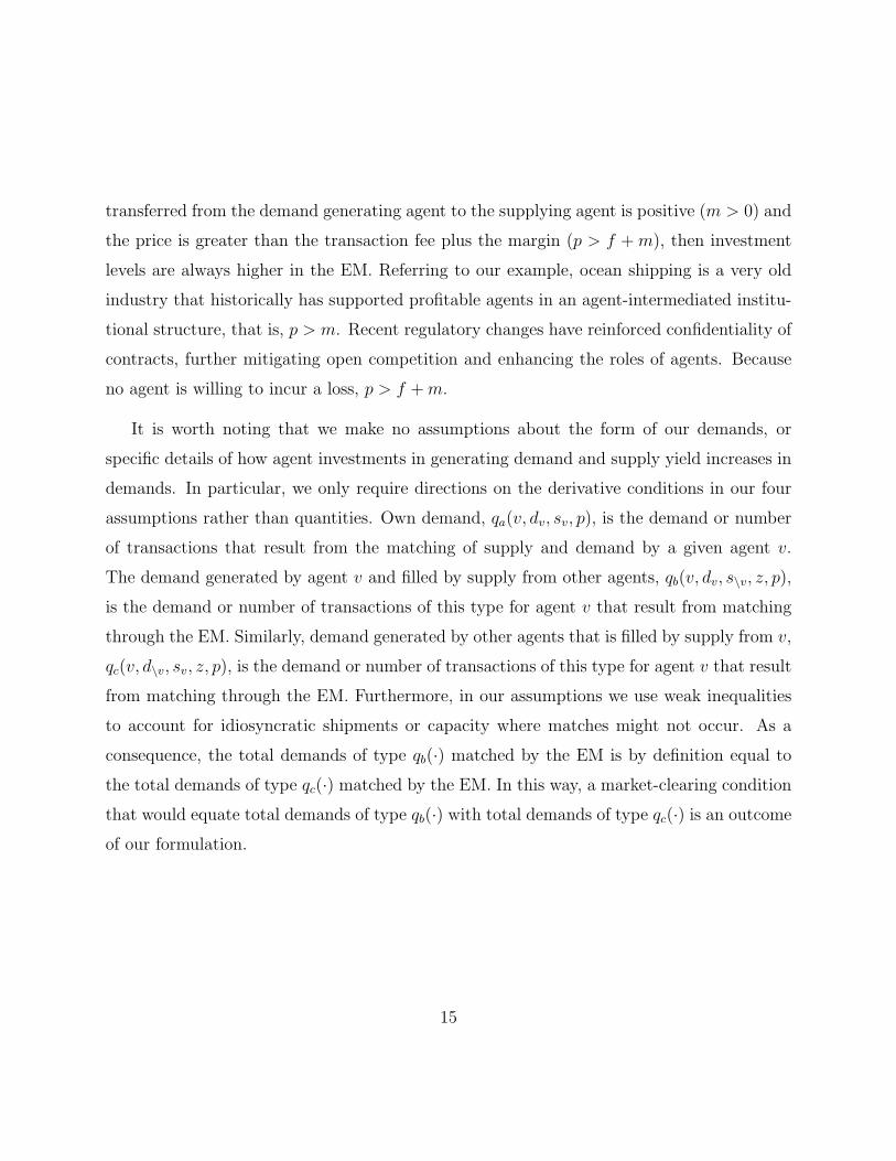
It is worth noting that we make no assumptions about the form of our demands, or

specific details of how agent investments in generating demand and supply yield increases in

demands. In particular, we only require directions on the derivative conditions in our four

assumptions rather than quantities. Own demand, qa(v, dv, sv, p), is the demand or number

of transactions that result from the matching of supply and demand by a given agent v.

The demand generated by agent v and filled by supply from other agents, qb(v, dv, s\v, z, p),

is the demand or number of transactions of this type for agent v that result from matching

through the EM. Similarly, demand generated by other agents that is filled by supply from v,

qc(v, d\v, sv, z, p), is the demand or number of transactions of this type for agent v that result

from matching through the EM. Furthermore, in our assumptions we use weak inequalities

to account for idiosyncratic shipments or capacity where matches might not occur. As a

consequence, the total demands of type qb(·) matched by the EM is by definition equal to

the total demands of type qc(·) matched by the EM. In this way, a market-clearing condition

that would equate total demands of type qb(·) with total demands of type qc(·) is an outcome

of our formulation.

15

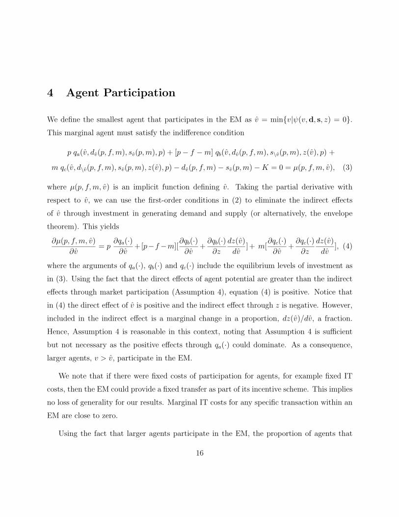
4 Agent Participation

We define the smallest agent that participates in the EM as v̂ = min{v|ψ(v,d, s, z) = 0}.This marginal agent must satisfy the indifference condition

p qa(v̂, dv̂(p, f,m), sv̂(p,m), p) + [p− f −m] qb(v̂, dv̂(p, f,m), s\v̂(p,m), z(v̂), p) +

m qc(v̂, d\v̂(p, f,m), sv̂(p,m), z(v̂), p)− dv̂(p, f,m)− sv̂(p,m)−K = 0 = µ(p, f,m, v̂), (3)

where µ(p, f,m, v̂) is an implicit function defining v̂. Taking the partial derivative with

respect to v̂, we can use the first-order conditions in (2) to eliminate the indirect effects

of v̂ through investment in generating demand and supply (or alternatively, the envelope

theorem). This yields

∂µ(p, f,m, v̂)

∂v̂= p

∂qa(·)∂v̂

+[p−f−m][∂qb(·)∂v̂

+∂qb(·)∂z

dz(v̂)

dv̂]+ m[

∂qc(·)∂v̂

+∂qc(·)∂z

dz(v̂)

dv̂], (4)

where the arguments of qa(·), qb(·) and qc(·) include the equilibrium levels of investment as

in (3). Using the fact that the direct effects of agent potential are greater than the indirect

effects through market participation (Assumption 4), equation (4) is positive. Notice that

in (4) the direct effect of v̂ is positive and the indirect effect through z is negative. However,

included in the indirect effect is a marginal change in a proportion, dz(v̂)/dv̂, a fraction.

Hence, Assumption 4 is reasonable in this context, noting that Assumption 4 is sufficient

but not necessary as the positive effects through qa(·) could dominate. As a consequence,

larger agents, v > v̂, participate in the EM.

We note that if there were fixed costs of participation for agents, for example fixed IT

costs, then the EM could provide a fixed transfer as part of its incentive scheme. This implies

no loss of generality for our results. Marginal IT costs for any specific transaction within an

EM are close to zero.

Using the fact that larger agents participate in the EM, the proportion of agents that

16

participate in the EM can be written as

z(v̂) =∫ v

v̂h(v)dv (5)

which is decreasing in v̂. From (3) the indifferent agent is a function of the price, the

transaction fee and the margin: v̂(p, f,m). Thus, z(v̂) ≡ z(p, f,m).

To determine the optimal settings of the transaction fee and the margin it is necessary to

determine the effects of changes in these EM choice variables on the proportion of agents that

participate in, and on the volume processed by, the EM. To shorten our notation we substi-

tute v̂(·) for v̂(p, f,m). Similarly for the proportion of agents that participate, z(p, f,m), we

use z(·). Lemma 1 determines the impact of the transaction fee on the proportion of agents

that participate in the EM.

Lemma 1: The proportion of agents that participate in the EM is decreasing in the trans-

action fee.

Proof: From (5) the changes in the proportion of agents that participate in the EM as a

result of changes in the transaction fee is dz(·)/df = −h(v̂(·))[∂v̂(·)/∂f ]. The impact of an

increase in the transaction fee through v̂(·) can be determined through the implicit function

rule using the indifference condition µ(p, f,m, v̂) = 0 from (3). That is, from the implicit

function theorm

∂v̂(·)/∂f = −∂µ(p, f,m, v̂)/∂v̂

∂µ(p, f,m, v̂)/∂f.

The sign of the numerator is positive from (4). The denominator is

∂µ(p, f,m, v̂)

∂f= −qb(·) +m

∂qc(·)∂d\v̂

∂d\v̂(·)∂f

< 0

where the arguments are as in (3). This results in ∂v̂(·)/∂f > 0. Substituting back in in

dz(·)/df results in dz(·)/df < 0. Q.E.D.

17

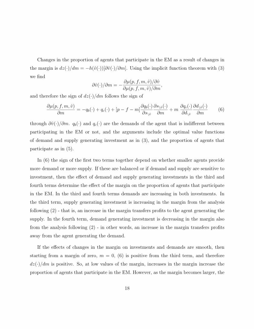
Changes in the proportion of agents that participate in the EM as a result of changes in

the margin is dz(·)/dm = −h(v̂(·))[∂v̂(·)/∂m]. Using the implicit function theorem with (3)

we find

∂v̂(·)/∂m = − ∂µ(p, f,m, v̂)/∂v̂

∂µ(p, f,m, v̂)/∂m,

and therefore the sign of dz(·)/dm follows the sign of

∂µ(p, f,m, v̂)

∂m= −qb(·) + qc(·) + [p− f −m]

∂qb(·)∂s\v̂

∂s\v̂(·)∂m

+m∂qc(·)∂d\v̂

∂d\v̂(·)∂m

(6)

through ∂v̂(·)/∂m. qb(·) and qc(·) are the demands of the agent that is indifferent between

participating in the EM or not, and the arguments include the optimal value functions

of demand and supply generating investment as in (3), and the proportion of agents that

participate as in (5).

In (6) the sign of the first two terms together depend on whether smaller agents provide

more demand or more supply. If these are balanced or if demand and supply are sensitive to

investment, then the effect of demand and supply generating investments in the third and

fourth terms determine the effect of the margin on the proportion of agents that participate

in the EM. In the third and fourth terms demands are increasing in both investments. In

the third term, supply generating investment is increasing in the margin from the analysis

following (2) - that is, an increase in the margin transfers profits to the agent generating the

supply. In the fourth term, demand generating investment is decreasing in the margin also

from the analysis following (2) - in other words, an increase in the margin transfers profits

away from the agent generating the demand.

If the effects of changes in the margin on investments and demands are smooth, then

starting from a margin of zero, m = 0, (6) is positive from the third term, and therefore

dz(·)/dm is positive. So, at low values of the margin, increases in the margin increase the

proportion of agents that participate in the EM. However, as the margin becomes larger, the

18

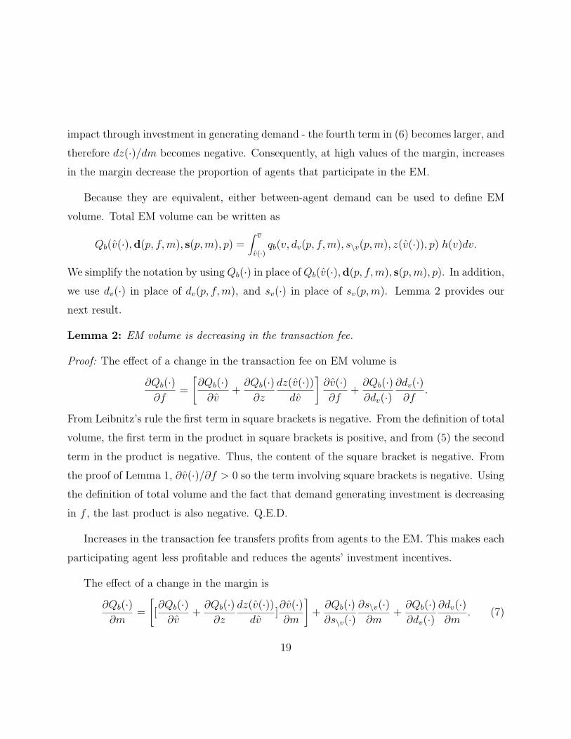
impact through investment in generating demand - the fourth term in (6) becomes larger, and

therefore dz(·)/dm becomes negative. Consequently, at high values of the margin, increases

in the margin decrease the proportion of agents that participate in the EM.

Because they are equivalent, either between-agent demand can be used to define EM

volume. Total EM volume can be written as

Qb(v̂(·),d(p, f,m), s(p,m), p) =∫ v

v̂(·)qb(v, dv(p, f,m), s\v(p,m), z(v̂(·)), p) h(v)dv.

We simplify the notation by usingQb(·) in place ofQb(v̂(·),d(p, f,m), s(p,m), p). In addition,

we use dv(·) in place of dv(p, f,m), and sv(·) in place of sv(p,m). Lemma 2 provides our

next result.

Lemma 2: EM volume is decreasing in the transaction fee.

Proof: The effect of a change in the transaction fee on EM volume is

∂Qb(·)∂f

=

[∂Qb(·)∂v̂

+∂Qb(·)∂z

dz(v̂(·))dv̂

]∂v̂(·)∂f

+∂Qb(·)∂dv(·)

∂dv(·)∂f

.

From Leibnitz’s rule the first term in square brackets is negative. From the definition of total

volume, the first term in the product in square brackets is positive, and from (5) the second

term in the product is negative. Thus, the content of the square bracket is negative. From

the proof of Lemma 1, ∂v̂(·)/∂f > 0 so the term involving square brackets is negative. Using

the definition of total volume and the fact that demand generating investment is decreasing

in f , the last product is also negative. Q.E.D.

Increases in the transaction fee transfers profits from agents to the EM. This makes each

participating agent less profitable and reduces the agents’ investment incentives.

The effect of a change in the margin is

∂Qb(·)∂m

=

[[∂Qb(·)∂v̂

+∂Qb(·)∂z

dz(v̂(·))dv̂

]∂v̂(·)∂m

]+∂Qb(·)∂s\v(·)

∂s\v(·)∂m

+∂Qb(·)∂dv(·)

∂dv(·)∂m

. (7)

19

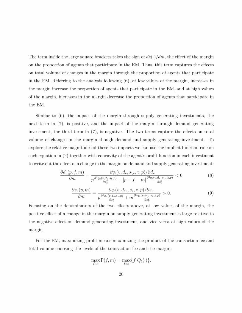
The term inside the large square brackets takes the sign of dz(·)/dm, the effect of the margin

on the proportion of agents that participate in the EM. Thus, this term captures the effects

on total volume of changes in the margin through the proportion of agents that participate

in the EM. Referring to the analysis following (6), at low values of the margin, increases in

the margin increase the proportion of agents that participate in the EM, and at high values

of the margin, increases in the margin decrease the proportion of agents that participate in

the EM.

Similar to (6), the impact of the margin through supply generating investments, the

next term in (7), is positive, and the impact of the margin through demand generating

investment, the third term in (7), is negative. The two terms capture the effects on total

volume of changes in the margin though demand and supply generating investment. To

explore the relative magnitudes of these two impacts we can use the implicit function rule on

each equation in (2) together with concavity of the agent’s profit function in each investment

to write out the effect of a change in the margin on demand and supply generating investment:

∂dv(p, f,m)

∂m=

∂qb(v, dv, s\v, z, p)/∂dv

p∂2qa(v,dv ,sv ,p)∂d2

v+ [p− f −m]

∂2qb(v,dv ,s\v ,z,p)

∂d2v

< 0 (8)

∂sv(p,m)

∂m=

−∂qc(v, d\v, sv, z, p)/∂sv

p∂2qa(v,dv ,sv ,p)∂s2

v+m

∂2qc(v,d\v ,sv ,z,p)

∂s2v

> 0. (9)

Focusing on the denominators of the two effects above, at low values of the margin, the

positive effect of a change in the margin on supply generating investment is large relative to

the negative effect on demand generating investment, and vice versa at high values of the

margin.

For the EM, maximizing profit means maximizing the product of the transaction fee and

total volume choosing the levels of the transaction fee and the margin:

maxf,m

Γ(f,m) = maxf,m

{f Qb(·)}.

20

The first-order conditions for maximizing profit are

∂Γ(f,m)

∂f= Qb(·) + f

∂Qb(·)∂f

= 0 and∂Γ(f,m)

∂m= f

∂Qb(·)∂m

= 0. (10)

An interior solution requires ∂Qb(·)/∂m be increasing at low values of the margin and be

decreasing at high values of the margin. This is likely from the two separate effects in

(7) described above: at low values of the margin, a change in the margin increases the

effect on total volume through increased participation in the EM and through a greater

relative impact on supply generating investment compared to demand generating investment.

At high levels of the margin a change in the margin decreases the effect on total volume

through reduced participation in the EM and through greater impact on demand generating

investment relative to supply generating investment. Thus, EM profits are maximized by

limiting agent participation. This key result is our first theorem.

Theorem 1: (Limited Market Participation) If total volume is increasing in the margin

at low values of the margin and is decreasing in the margin at high values of the margin,

then EM profits are maximized by limiting agent participation.

Proof: From the second first-order condition in (10), we require that ∂Qb(·)/∂m = 0 in

(7). From (8) and (9), the last two products in (7) are offsetting in sign, and are of similar

magnitude. For ∂Qb(·)/∂m = 0 the remaining term in (7), depends on the sign of dz(·)/dm,

must balance the offsetting difference in (8) and (9), and this difference is small. At low

values of m, dz(·)/dm > 0, increasing the proportion of agents that participate. As m

increases, dz(·)/dm becomes negative, decreasing the proportion of agents that participate.

Q.E.D.

The EM’s optimization problem does not maximize the proportion of agents that partici-

pate. This is because changes in the margin have opposite effects on equilibrium investments

in generating demand and in generating supply. An increase in the margin reduces the in-

centives to invest in generating demand and increases incentives in generating supply. This

21

impacts not only the direct effects of demand and supply generating investment on EM

volume, but also the indirect effect of the proportion of agents that participate in the EM.

Therefore, the EM improves service not only by providing a matching mechanism for supply

and demand, but also by providing the right combination of investment incentives to bal-

ance the generation of supply and demand. Limiting agent participation is critical for the

EM’s profit maximizing when demand investments are important. In this case, the margin

is set low to incent investments from larger agents, and smaller agents may not make enough

through the EM to cover their operating costs.

Our theorem is related to results in [5] and [6]. Their results, whereby in a buyer-

supplier IT framework it could be optimal for buyers to limit participation by suppliers,

derive from the need to provide suppliers with an adequate incentive to invest. In their

work the incentive was necessary to induce suppliers to invest in non-contractible IT assets.

In our model the EM must provide investment incentives for agents to generate demand

and supply because each agent’s expertise is different and unobservable to the EM. We

also note that these investment incentives for agents to generate demand and supply reduce

the uncertainty of matching demand and supply through pooling because this investment

increases the probability of matching a given shipment with capacity.

Each agent has the choice of participating in the EM, or not participating in the EM but

be active in the traditional market, or be inactive. The Corollary to Theorem 1 indicates

the breakdown.

Corollary: All agents that are active in the traditional market participate in the EM. More

agents participate in the EM than are active in the traditional market.

Proof: Comparing agent profits in the EM versus the traditional market, ψ(v,d, s, z) versus

π(v, dv, sv), and noting that investment levels are always higher in the EM, an agent could

set investments to the equilibrium levels from the traditional market and be better off in the

22

EM. Define the smallest active agent in the traditional market as the smallest agent with

zero profits, v̌ = min{v|π(v, dv, sv) = 0}. π(v, dv, sv) is increasing in v so in the traditional

market larger agents, v > v̌, are active. Because of the additional value provided by the EM,

ψ(v̌,d, s, z(v̌)) > π(v̌, dv̌, sv̌) = 0. Therefore v̂ > v̌ meaning more agents participate in the

EM. Q.E.D.

This corollary is important because it indicates that the EM draws agents into the in-

dustry that would otherwise not be generating either shipments or capacity. Indeed, this

is particularly crucial in an industry such as international freight transportation where sig-

nificant unsatisfied demand exists. In practice the increase in agent participation is also an

increase in the different niche markets served by this industry.

5 Endogenous Price and Welfare

5.1 Impact on the Price

So far we have considered the price as fixed by conditions outside of the EM such that

both individual agents and the industry are price-takers. Although agents may not be

able to influence the price individually, their aggregate investments in generating demand

and supply may impact the price because they may change the balance between demand

and supply. Endogenizing price means incorporating the difference between investments in

generating demand and investments in generating supply.

Let the balance between demand and supply generating investment be represented by

the vector of differences in investment: ~δ(f,m) = d(p, f,m) − s(p,m). Recall that invest-

ments in generating demand are decreasing in the transaction fee and the margin, f and m,

and investments in generating supply are increasing in the margin, m. Directly from the

properties of these investment functions, each vector element of ~δ(f,m) is decreasing in the

23

transaction fee and the margin.

Let ρ(f,m) be the price that aggregates the effects of the transaction fee and the margin

from ~δ(f,m). The price ρ(f,m) captures the effects of the transaction fee and the margin on

the balance between demand and supply. The price must have the same properties as ~δ(f,m),

namely ρ(f,m) is decreasing in the transaction fee because the increases in the transaction

fee reduces demand generating investment. Similarly, the price ρ(f,m) is decreasing in the

margin because increases in the margin reduce demand generating investment and increase

supply generating investment.

Using this form of price makes price endogenous. That is, price depends on the EM’s

choice variables f and m. We can rewrite total volume by replacing p with ρ(f,m). To

simply the notation we let the demand generating investment vector d(ρ(f,m), f,m) be

written as d(·), the supply generating investment vector s(ρ(f,m),m) be written as s(·),agent v’s demand generating investment dv(ρ(f,m), f,m) be written as dv(·), and v’s supply

generating investment s\v(ρ(f,m),m) be written as s\v(·). Total volume with endogenized

price is then

Q̃b(v̂(·),d(·), s(·), ρ(f,m)) =∫ v

v̂(·)qb(v, dv(·), s\v(·), z(v̂(·)), ρ(f,m)) h(v)dv.

With total volume so defined, we can provide our last theorem followed by a corollary that

describes the resulting effects on price.

Theorem 2: (Endogenous Price) If the total effect of an increase in the price on total

volume is positive, then the optimal transaction fee and margin are lower when price is

endogenous than they are when price is determined outside the EM. Otherwise, the optimal

transaction fee and margin are higher when price is endogenous than they are when price is

determined outside the EM.

Corollary: If the total effect of an increase in price on total volume is positive, then the

24

endogenous price is higher than the price determined outside the EM. Otherwise, the endoge-

nous price is lower than the price determined outside the EM.

Proof: We simplify the notation using Q̃b(·) in place of Q̃b(v̂(·),d(·), s(·), ρ(f,m)).

It is not possible to compare total volume with the endogenous price and with the price de-

termined outside the EM, Q̃b(·) and Qb(·), without a fixed point where the endogenous price

ρ(f0,m0) = p for the pair (f0,m0). However, the interior optimal solution for maxf,m Γ(f,m),

profits when the price is determined outside the EM, provides such a fixed point. We use

this to compare the optimal transaction fee and margin.

Let f ∗ and m∗ be the interior optimal solution to maxf,m Γ(f,m) = f Qb(·), the EM

profits when price is determined outside the EM. Use this optimum to fix the point p =

ρ(f ∗,m∗) where the prices are equal, so at that point EM volume in the two cases is equal

Qb(·) = Q̃b(·) at (f ∗,m∗). The necessary first-order conditions for the interior optimum with

the determined outside the EM price are as in (10), yielding (f ∗,m∗).

Denote profits when price is endogenous as Γ̃(f,m). Evaluated at (f ∗,m∗) we have

∂Γ̃(f,m)

∂f ∗ = Q̃b(·) + f ∗ dQ̃b(·)df∗ = Q̃b(·) + f ∗ [

∂Qb(·)∂f ∗ +

dQ̃b(·)dρ

∂ρ(f ∗,m∗)

∂f ∗ ]

and∂Γ̃(f,m)

∂m∗ = f ∗ dQ̃b(·)dm∗ = f ∗ [

∂Qb(·)∂m∗ +

dQ̃b(·)dρ

∂ρ(f ∗,m∗)

∂m∗ ],

where ∂Qb(·)/∂f ∗ and ∂Qb(·)/∂m∗ represent the direct effects of changes in the transaction

fee and the margin like those in (10). The remaining terms are the indirect effects of the

transaction fee and the margin through price. If the total effect of an increase in price on

total volume is positive, dQ̃b(·)/dρ > 0, then both ∂Γ̃(f,m)/∂f ∗ and ∂Γ̃(f,m)/∂m∗ are

negative.

The second-order conditions for an interior optimum require concavity in each variable.

Thus, if both ∂Γ̃(f,m)/∂f ∗ and ∂Γ̃(f,m)/∂m∗ are negative, then the decision variables

25

have been set too high and optimizing profits when price is endogenously determined (as

represented by the first-order conditions) requires a transaction fee lower than f ∗ and a

margin lower than m∗. Proof of the converse is straightforward. Q.E.D.

Theorem 2 and its corollary embody our second key result: the agent-intermediated EM

can cause both volume and price to increase simultaneously. Theorem 2 and its corollary

depend on the impact of the price on total volume, and thus on individual agent demands.

Referring to the arguments of Q̃b(·), a change in price has four separate effects. The first is an

indeterminate indirect effect through agent participation - similar to but more complex than

the one in (6). The second is the negative indirect effect through investments in generating

demand. The third is the positive indirect effect through investments in generating supply.

And finally, there is a negative direct effect of price on volume.

An increased price is normally associated with decreased volume. However, here an in-

creased price has a positive indirect effect through supply-generating investment and possibly

a positive indirect effect through participation, which can simultaneously result in increased

volume. That is, if the demand-supply balance is such that identifying and bringing addi-

tional supply to the market can increase the number of transactions, then an increase in

price can motivate agents to bring that additional supply to market. Due to the conflicting

set of direct effects and indirect effects through demand and supply generating investments,

it is not possible to determine in general if endogenizing price increases or decreases profits

for the EM and for the individual agents.

5.2 Effects on Welfare

When price is determined by conditions outside the EM, the effects of the EM on welfare are

positive. Four groups of stakeholders must be accounted for: buyers, sellers, agents, and the

EM - where in ocean shipping the first two would be shippers and carriers respectively. If

26

the fixed costs of agents and the EM are covered, Qb(·) > 0 implies that each of the groups

complete transactions they otherwise would not - at the same price - and are therefore better

off. Thus, the EM is not only welfare enhancing, it is Pareto optimal for all stakeholders.

Although this should be true given that the EM effectively relaxes a constraint in the opti-

mization program for the market, what is important is the way in which each stakeholder

benefits.

When price is endogenous - affected by agent investments - the effects of the EM on

welfare are less clear. In addition to the direct effects of price on demands, changes in

price also have investment impacts on volume through changes in the transaction fee and

the margin. However, as we saw in Theorem 2, the direction of these changes - and hence

incentives for investment - depend on the sign of the direct effect of a change in price on

total volume.

Even ignoring the investment effects, the outcome is equivocal. Consider, for example,

when the presence of the EM increases price. Buyers benefit from completing transactions

through the EM that would not have been completed otherwise. Nonetheless, those transac-

tions that would have been completed without the EM now face a higher price. Hence, the

aggregate impact on the welfare of buyers is mixed. Sellers face a similar tradeoff. Volume is

increased by those transactions that occur through the EM. Unfortunately, transactions not

requiring the EM face an increased price, reducing the off-EM volume for sellers compared to

the traditional market. This reduction may more than offset the new volume from the EM.

Similarly, agents that participate in the EM gain from the transactions on the EM, but lose

off-EM volume compared to the traditional market. Those agents that do not participate

in the EM simply lose volume and the lower profits that result may not be offset by the

increased price.

Alternatively, when presence of the EM decreases price, buyers gain from completing

27

transactions through the EM that they would not complete otherwise, and also gain from

lower prices on those transactions completed without the EM. Sellers also benefit from the

EM transactions and higher volumes as compared to the traditional market from the lower

price. For both buyers and sellers, however, these gains may be negated by a reduced

incentive for demand and supply generating investment. The impact on agents is mixed:

those that participate in the EM may gain from transactions over the EM, but those that do

not participate may be less profitable because of the reduced price - even at higher volumes.

So long as its fixed costs are covered, the agent-intermediated EM is profitable. Making

the EM profitable is critical to motivate the needed investment in IT infrastructure to sup-

port the development of the centralized repository for demand and supply information. In

particular, this investment can be costly since the special information requirements for this

market - the specificity and perishability of demand and supply - are more extensive than

for financial or commodity markets.

6 Conclusion

We have shown that with price determined by the general freight transportation marketplace,

an agent-intermediated EM increases agent participation and investment. The importance

of agent investment is highlighted by the EM’s allocation of profits between demand and

supply providing agents on a given transaction whereby the EM balances participation and

investment effects in its allocation, consequently restricting agent participation in the market.

This restriction of participation is different than what one expects of commodity markets,

where market depth and liquidity would suggest greater participation is more profitable for

the EM.

When price is endogenous - influenced by the demand and supply balance in the EM,

28

we found that if price increases supply generating investment and participation, then price

and volume on the EM can increase simultaneously. This result is different from what we

might expect in a standard microeconomic analysis. Finally, since an endogenous price can

be higher or lower with an agent-intermediated EM, the EM may not be welfare enhancing

for all the stakeholders.

The driving force behind both our key results is the impact of an EM on agent investment.

One important managerial implication for agents is that the agent-intermediated EM changes

the returns to different investments. In the traditional market an agent must invest in

matching its own demand and supply - for example, once a shipment (demand) is secured,

the agent must invest in finding capacity (supply) for that shipment in order to obtain a

return on investment. In an EM an agent can obtain an immediate return on investment from

generating a single side of the transaction - for example, securing a shipment whose capacity

is provided by another agent through the EM. One consequence of the change in returns to

investment brought about by the EM is that agents are rewarded for specialization, whereby

agents may focus on a particular side of the transaction and a specific niche in that side of

the transaction. For example, an agent using an EM may focus its investment on shippers

that ship automobiles to the US from Europe rather than having to split its investment

between shippers and carriers. This increases the differentiation among agents, providing

them with higher profits. Competition among agents ultimately reappears through price -

the price that is determined via changes in the demand and supply balances in the EM.

Nonetheless, we recognize that our assumption of non-competition in agent investments

is a strong assumption. This assumption could be relaxed for the demands generated by one

agent and filled by another agent. In the case of an agent providing demand filled by supply

from other agents (qb(·)) for example, the relaxation could take the form of including own

investment in generating supply because the effect of that investment could be to enable

to agent to both generate and fill the demand, thereby moving that particular transaction

29

to own demand. However, competition between agents in demand generating or supply

generating investments within our approach to a Nash equilibrium would violate our super-

modularity conditions. In that case, another approach using quasiconcavity conditions may

yield several of our results, but at the expense of additional assumptions.

With an agent-intermediated EM individual agents will eventually be forced out of us-

ing the traditional market exclusively because the change in the structure of the returns

to agent investments brought about by the EM will make agents that join the EM more

profitable through an increase in transaction volume. This will increase the liquidity of the

freight transportation marketplace for those agents on the EM. Indeed, the EM may increase

price and transaction volume simultaneously. Thus, participating in the EM will become a

strategic necessity.

For the EM the critical issue is the balance between providing incentives for agent in-

vestment and opening the market to broad agent participation. The EM effectively balances

profits from investments by larger agents with increased volume from greater participation -

the setting of the margin determines investments by agents and which agents are profitable

by participating in the EM. Therefore, calibrating the level of the margin divided between

agents is fundamental to the performance of the EM.

7 Acknowledgements

Helpful suggestions have been provided by the Guest Editor and two anonymous Review-

ers, seminar participants at Penn State University, Michigan State University, The Ohio

State University, University of Southern California, University of Wisconsin-Madison, Uni-

versity of Oregon, University of Pittsburgh, and participants at WISE. We especially thank

Clive Wrigley and John King for discussions about freight transportation. We also thank

30

the National Science Foundation, the Natural Science and Engineering Research Council of

Canada, the Social Science and Humanities Research Council of Canada, and the Informatics

Research Centre at the University of Calgary for support.

8 References

[1] R. Alt, P. Forster, and J.L. King, The Great Reversal: Information and Transportation

Infrastructure in the Intermodal Vision. Proceedings of the National Conference on Setting

an Intermodal Transportation Research Framework, National Academy Press, Washington

D.C., 31-53 (1997).

[2] S. Ba, Whinston, A.B., and H. Zhang, Building Trust in the Electronic Market Through an

Economic Incentive Mechanism, Proceedings of the Twentieth International Conference on

Information Systems, De, P. and DeGross, J.I. (eds.), Charlotte, North Carolina (December

1999).

[3] J.P. Bailey and Y. Bakos, An Exploratory Study of the Emerging Role of Electronic

Intermediaries, International Journal of Electronic Commerce, 1, 3, 7-20 (Spring 1997).

[4] J.Y. Bakos, The Emerging Role of Electronic Marketplaces on the Internet, Communica-

tions of the ACM, 41, 8, 35-42 (August 1998).

[5] J.Y. Bakos and E. Brynjolfsson, From Vendors to Partners: Information Technology and

Incomplete Contracts in Buyer-Supplier Relationships, Journal of Organizational Comput-

ing, 3, 3, 301-328 (1993).

[6] R.D. Banker, J. Kalvenes and R.A. Patterson, Information Technology, Contract Com-

pleteness, and Buyer-Supplier Relationships, Proceedings of the Twenty-First International

Conference on Information Systems, De, P. and DeGross, J.I. (eds.), Brisbane, Australia,

31

218-228 (December 2000)

[7] A.M. Chircu, G.B. Davis and R.J. Kauffman, The Role of Trust and Expertise in the

Adoption of Electronic Commerce Intermediaries, MISRC Working Paper, March 2000).

[8] E.K. Clemons and B.W. Weber, Alternative Securities Trading Systems: Tests and Reg-

ulatory Implications of the Adoption of Technology, Information Systems Research, 7, 2,

163-188 (June 1996).

[9] DAT Services, http://www.dat.com (1999).

[10] P. Forster and J.L. King, Information Infrastructure Standards in Heterogeneous Sectors:

Lessons from the Worldwide Air Cargo Community, In Standards Policy for Information

Infrastructure, B. Kahin and J. Abbate eds., MIT Press, Cambridge, MA. (1995).

[11] R. Gellman, Disintermediation and the Internet, Government Information Quarterly,

13, 1, 1-8 (1996).

[12] GT Nexus, http://www.tradient.com/about (2001).

[13] M. Halper, Meet the New Middlemen, Computerworld, 31, 17, C10-C14 (April 28, 1997).

[14] F.A. Hayek, The Use of Knowledge in Society, American Economic Review, 35, 4, 519-

530 (September 1945).

[15] T. Hoffman, No More Middlemen, Computerworld, 55 (July 17, 1995).

[16] H.G. Lee, Do Electronic Marketplaces Lower the Price of Goods? Communications of

the ACM, 41, 1, 73-80 (January 1998).

[17] I. Lewis and D.B. Vellenga, The Ocean Shipping Reform Act of 1998, Transportation

Journal, 39, 4, 27-34 (Summer 2000).

[18] K. Lynch, The 7 Immutable Laws of Collaborative Logistics, World Trade, 13, 10, 86-90

32

(October 2000).

[19] P. Milgrom and J. Roberts, Rationalizability, Learning, and Equilibrium in Games with

Strategic Complementarities, Econometrica, 58, 6, 1255-1277 (November 1990).

[20] NTE, http://www.nte.net/PressRelease/28.html (1998).

[21] F.J. Riggins, C.H. Kriebel and T. Mukhopadhyay, The Growth of Interorganizational

Systems in the Presence of Network Externalities, Management Science, 40, 8, 984-998 (Au-

gust. 1994).

[22] N. Shashikumar and G.L. Schatz, The Impact of U.S. Regulatory Changes on Interna-

tional Intermodal Movements, Transportation Journal, 40, 1, 5-14 (Fall 2000).

[23] C.S. Sherwood and R. Bruns, Solving International Transportation Problems, Review

of Business, 14, 1, 25-30 (Summer/Fall 1992).

[24] D. Topkis, Equilibrium Points in Nonzero-Sum n-Person Submodular Games, Siam

Journal of Control and Optimization, 17, 6, 773-787 (November 1979).

[25] E.T.G. Wang and A. Seidmann, Electronic Data Interchange: Competitive Externalities

and Strategic Implementation Policies, Management Science, 41, 3, 401-418 (March 1995).

[26] R. Wigand and R. Benjamin, Electronic Commerce: Definition, Theory and Context,

The Information Society, 13, 1, 1-16 (1996).

[27] O.E. Williamson, The Economics of Organization: The Transaction Cost Approach,

American Journal of Sociology, 87, 3, 548-577 (1981).

[28] O.E. Williamson, The Economic Institutions of Capitalism: Firms, Markets, Relational

Contracting, New York: Free Press (1985).

33