Agenda

• Path smoothing• PID• Graph slam

Path smoothing• Until now we have worked with straight

motions

0 0.5 1 1.5 2 2.5 3 3.5 4 4.5 50

0.5

1

1.5

2

2.5

3

3.5

4

4.5

5

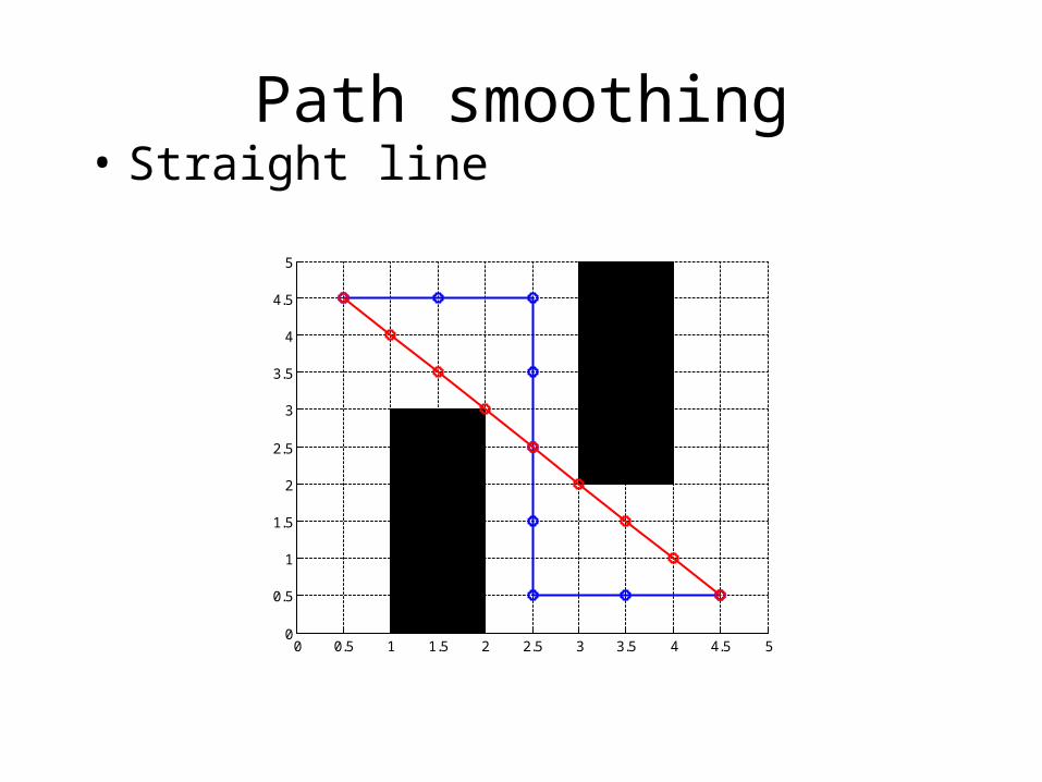
Path smoothing• Straight line

0 0.5 1 1.5 2 2.5 3 3.5 4 4.5 50

0.5

1

1.5

2

2.5

3

3.5

4

4.5

5

Path smoothing• Smooth line

0 0.5 1 1.5 2 2.5 3 3.5 4 4.5 50

0.5

1

1.5

2

2.5

3

3.5

4

4.5

5

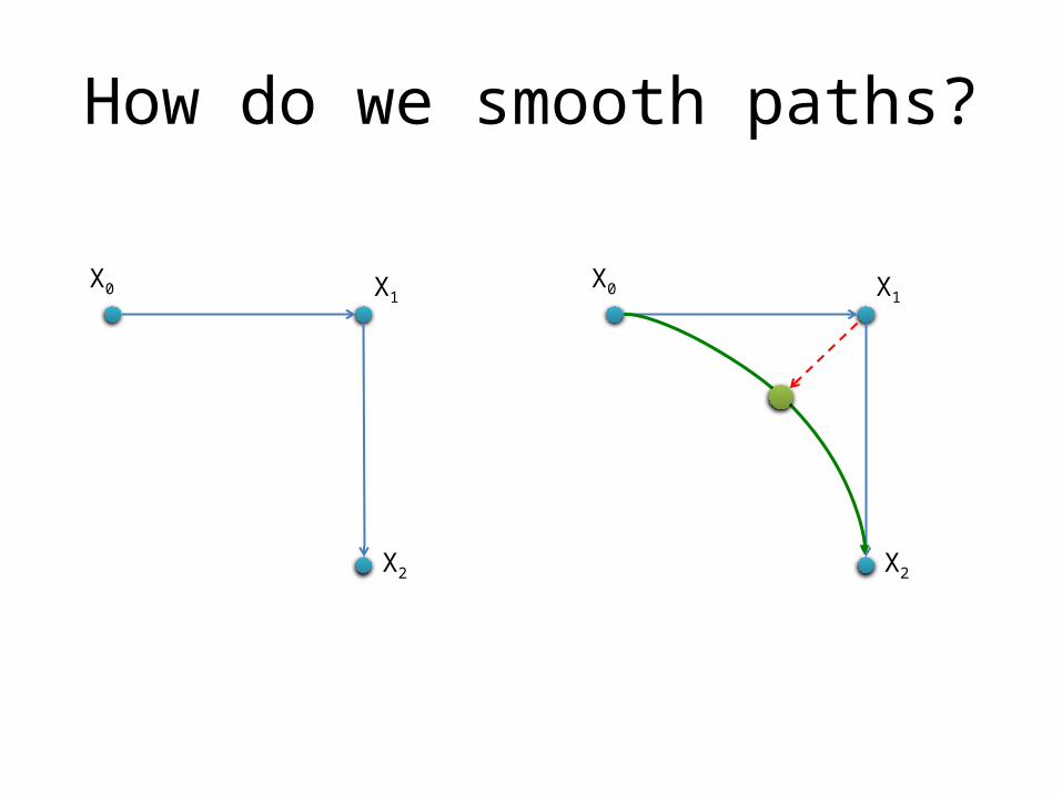
How do we smooth paths?

X0 X1

X2

X0 X1

X2

How do we smooth paths?

X0 X1

X2

As we move X1 in we reduce the distance between X1 and X0 and X1 and X2. In other words as we move X1 the length of the red lines get smaller.

So how do we figure out how to move X1 to reduce the length of the red lines?

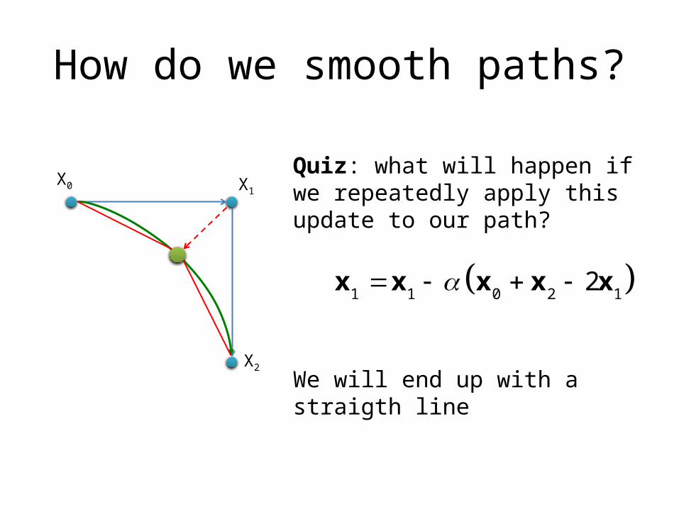
How do we smooth paths?

X0 X1

X2

We subtract X1 from each of its neighbours and add the difference to X1 . In other word:

1 1 0 1 2 1

1 1 0 2 12

x x x x x x

x x x x x

where α is a weight term that is used to control how quickly we move away from X1

How do we smooth paths?

X0 X1

X2

Quiz: what will happen if we repeatedly apply this update to our path?

1 1 0 2 12 x x x x x

We will end up with a straigth line

How do we smooth paths?

X0 X1

X2

Therefore we need a constraint to control the update to make it balance!

To do this we will iteratively move the point back towards the original point

Lets call the moving point Y1 to distinguish it from the original point X1

0 21 1 12 y x xy y

How do we smooth paths?

X0 X1

X2

We now define the counter weight, which drags the point Y1 back to the original position X1

1 1 11 y xy y

Additional terms

• Distance to wall• Fixed points• Similarity of two following segments

1x

1 1 2

1 1 2

i i i i i i

i i i i i i

x x x x x x

y y y y y y

1 1 2

1 1 2

i i i i i i

i i i i i i

x x x x x x

y y y y y y

Path smoothing Demo using gradient descent

D:\Skole\AU-TekniskIT\Kalman\Min præsentation\Eksempel\Path smooth demo\Pathsmooth.m

PID

PID controlling

Cross track error

Use the error to control the steering

Desired path

Closed loop control systems

• Use a measurement of output to control the input (Feedback)

PID control

P depends on the present error, I on the accumulation of past errors, D is a prediction of future errors,

e(t) = set point - process value

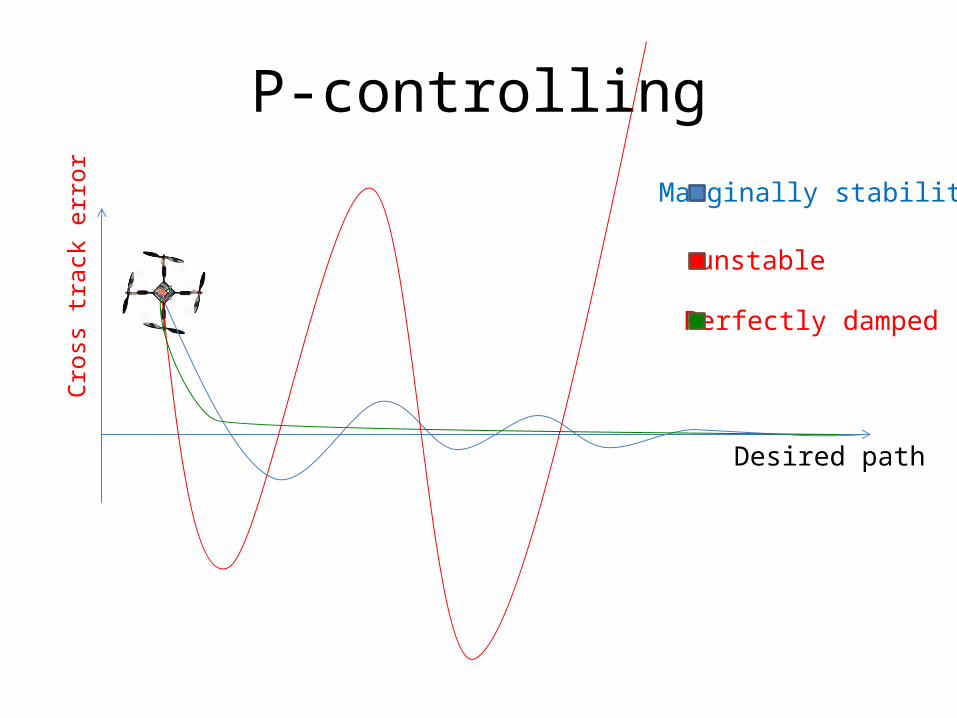
P-controllingCr

oss

trac

k er

ror Marginally stability

Desired path

unstable

Perfectly damped

Error term• The error term is derived by subtracting the

feedback (i.e. current position) from the set point (i.e. desired position).

• e(t) = u(t) – y(t)

Proportional Term• Simple proportional coefficient Kp is

multiplied by the error term.• Provides linear response to the error term.

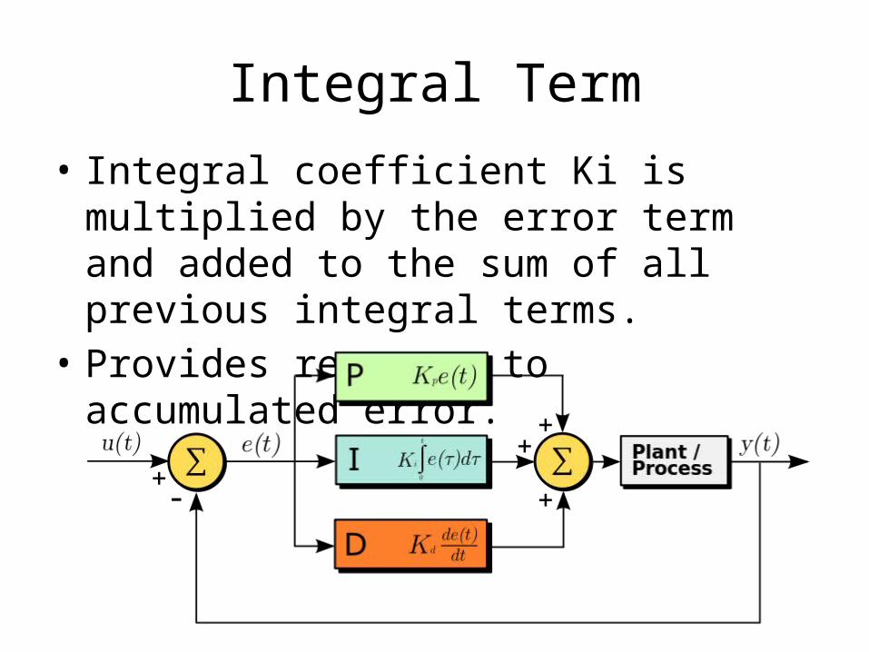
Integral Term• Integral coefficient Ki is multiplied by the error

term and added to the sum of all previous integral terms.

• Provides response to accumulated error.

Derivative Term• Derivative coefficient Kd is multiplied by the

difference between the previous error and the current error.

• The derivative term slows the rate of change of the controller output

Effects of increasing a parameter independently

Parameter Rise time Overshoot Settling time Steady-state error Stability

Decrease Increase Small change Decrease Degrade

Decrease Increase Increase Eliminate Degrade

Minor change Decrease Decrease No effect in theory

Improve if small

pK

IK

DK

Discrete PID algorithmprevious_error = setpoint - process_feedbackintegral = 0 while(1) {

wait(dt) error = setpoint - process_feedbackintegral = integral + (error*dt) derivative = (error - previous_error)/dtoutput = (Kp*error) + (Ki*integral) + (Kd*derivative) previous_error = error

}

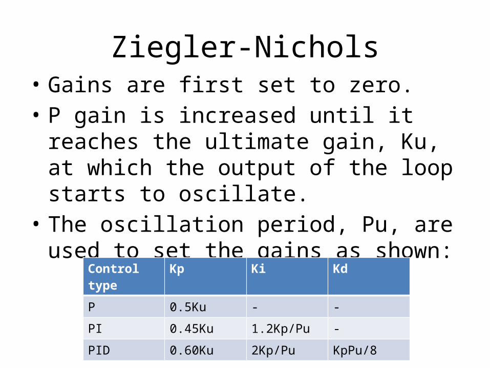
Ziegler-Nichols• Gains are first set to zero. • P gain is increased until it reaches the ultimate

gain, Ku, at which the output of the loop starts to oscillate.

• The oscillation period, Pu, are used to set the gains as shown:

Control type Kp Ki Kd

P 0.5Ku - -

PI 0.45Ku 1.2Kp/Pu -

PID 0.60Ku 2Kp/Pu KpPu/8

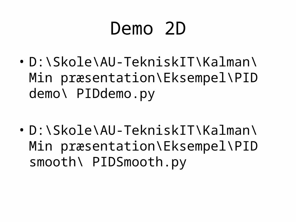
Demo 2D

• D:\Skole\AU-TekniskIT\Kalman\Min præsentation\Eksempel\PID demo\ PIDdemo.py

• D:\Skole\AU-TekniskIT\Kalman\Min præsentation\Eksempel\PID smooth\ PIDSmooth.py

= to be able to build a map of an environment and simultaneously localize within this map

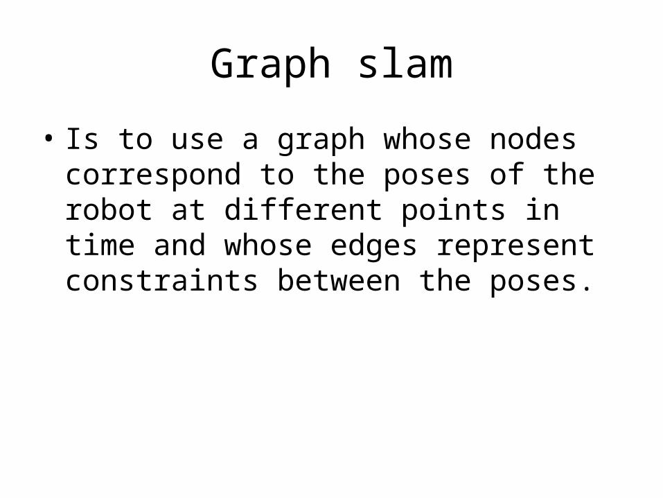
Graph slam

• Is to use a graph whose nodes correspond to the poses of the robot at different points in time and whose edges represent constraints between the poses.

Graph slam problem

• To estimate the posterior probability of the robot’s path and the map given all the measurements plus an the initial position

• Assumption: The world is static

1:Tx m

0x

1: 1: 1: 0, | , ,

T T Tp x m z u x

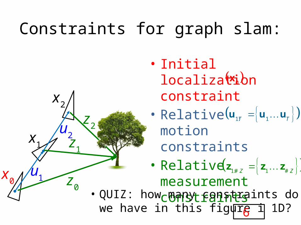
Constraints for graph slam:

• Initial localization constraint

• Relative motion constraints

• Relative measurement constraints

0x

1x

2x

0z

1z

2z

• QUIZ: how many constraints do we have in this figure i 1D? 6

1u

2u

0x

1: 1T Tu u u

1:# 1 #Z Zz z z

Implementation of Graph based slam

0X

TX

0Z #Z

Z

1X

TX

1Z

#ZZ

xy

xyxy

xy

x y x y x y x y

2 # 'T Z s

1

1

Implementation of Graph based slam

0X

TX

0Z #Z

Z

1X

TX

1Z

#ZZ

xy

xyxy

xy

x y x y x y x y

2 # 'T Z s

1

1

The best estimate

for all the robot locations and

landmark locations

Quiz: 1D Slam

0X 1

X0

Z1

Z

0X

1X

0Z

1Z

0 1

0 4

X X

44

1

1

11

0 1

0 1

4

4

X X

X X

Which cells will be modified?What will the values in the cells then be?

Quiz: 1D Slam

0X 1

X0

Z1

Z

0X

1X

0Z

1Z

1 0

0 3

X Z

4

41

1

11

12 1

1 3

7

1 0

1 0

3

3

X Z

X Z

Which cells will be modified?What will the values in the cells then be?

Quiz: 1D Slam

Which fields are not modifies?

0X 1

X0

Z1

Z

0X

1X

0Z

1Z

?

?

5

5

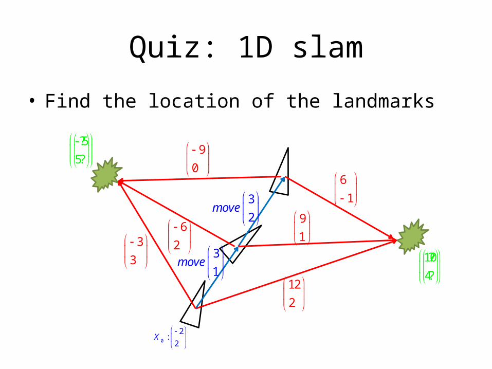
Quiz: 1D slam

0

2:

2X

• Find the location of the landmarks

3

1move

3

2move

3

3

6

2

9

0

?

?

12

2

9

1

6

1

10

4

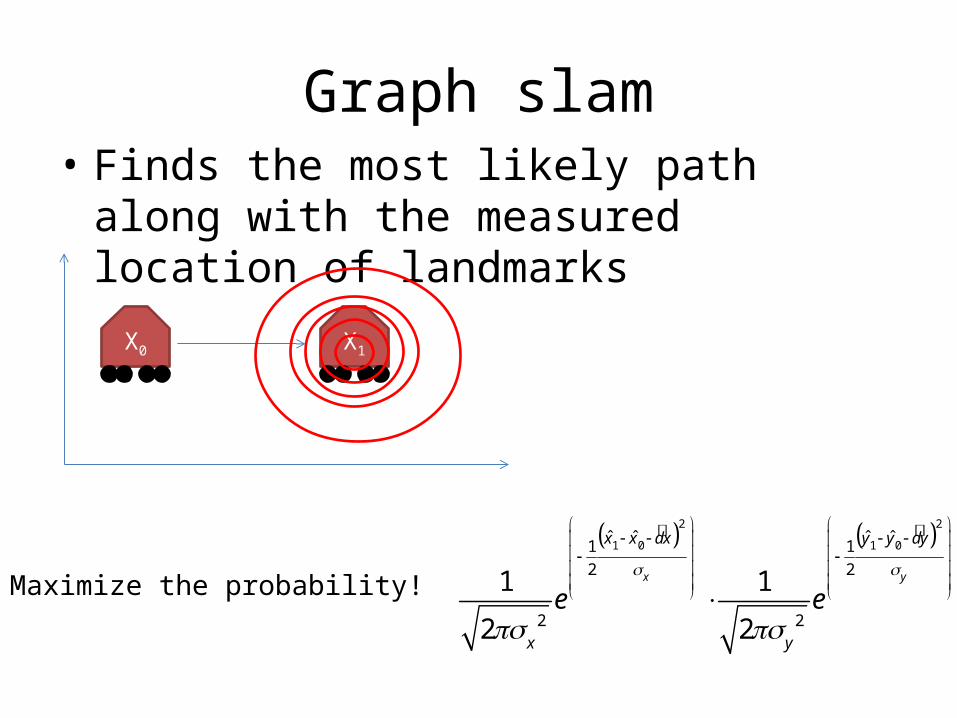
Graph slam• Finds the most likely path along with the

measured location of landmarks

X0 X1

2 2

1 0 1 0ˆ ˆ ˆ ˆ1 12 2

2 2

1 1

2 2

x y

x x dx y y dy

x y

e e

Maximize the probability!

Simplifying the probability maximization

2 2

1 0 1 1 1 1

1 1

1 1

ˆ ˆ ˆ ˆ ˆ1 12 2

2 2

1 1....

2 2

X Z

x x dx Z X X Z

X Z

e e

X0 X1 Z1

+

Finds the most likely path along with the measured location of landmarks

Demo with different measurement confidences

T0 T1

D:\Skole\AU-TekniskIT\Kalman\Min præsentation\Eksempel\Slam\slam.py

References

• https://www.udacity.com• http://www.comp.dit.ie/jkelleher/rtf/classmat

erial/week10/PathSmoothing.pdf