Agency Business Cycles∗

Mikhail GolosovPrinceton University and NBER

Guido MenzioUniversity of Pennsylvania and NBER

January 2017

Abstract

We develop a theory of endogenous and stochastic fluctuations in aggregate eco-nomic activity. Individual firms choose to randomize over firing or keeping workers whoperformed poorly in the past to give them an ex-ante incentive to perform. Differentfirms choose to correlate the outcome of their randomization to reduce the probabilitywith which they fire non-performing workers. Correlated randomization leads to aggre-gate fluctuations. Aggregate fluctuations are endogenous– they emerge because firmschoose to randomize and they choose to randomize in a correlated fashion– and theyare stochastic– they are the manifestation of a randomization process. The hallmarkof a theory of endogenous and stochastic fluctuations is that the stochastic process foraggregate “shocks”is an equilibrium object.

JEL Codes: D86, E24, E32.

Keywords: Endogenous and Stochastic Cycles, Coordinated Randomization, Unem-ployment Fluctuations.

∗Golosov: Department of Economics, Princeton University, 111 Fisher Hall, Princeton, NJ 08544 (email:golosov@princeton.edu); Menzio: Department of Economics, University of Pennsylvania, 3718 Locust Walk,Philadelphia, PA 19104 (email: gmenzio@sas.upenn.edu). We are grateful to Gadi Barlevy, Paul Beaudry,Katarina Borovickova, Veronica Guerrieri, Christian Haefke, Boyan Jovanovic, John Kennan, NarayanaKocherlakota, Ricardo Lagos, Rasmus Lentz, Igor Livschits, Nicola Pavoni, Thijs van Rens, Guillaume Ro-cheteau, Tom Sargent, Karl Shell, Ben Schoefer, Robert Shimer, Mathieu Taschereau-Dumouchel and RandyWright for comments on earlier drafts of the paper. We are also grateful to participants at seminars at theUniversity of Wisconsin Madison, New York University, University of Chicago, University of California Berke-ley, CREI, LSE, New York FRB, Minneapolis FRB, and at the Search and Matching European Conferencein Aix-en-Provence, the Search and Matching Workshop at the Philadelphia FRB, the conference in honorof Chris Pissarides at Sciences Po, the Econometric Society World Congress in Montreal, the NBER EFGMeeting at the New York FRB.

1

1 Introduction

What causes cyclical fluctuations in economic activity? This is one of the central questions in

macroeconomics and naturally it has attracted a great deal of attention from both theorists

and empiricists. One explanation for cyclical fluctuations is that the economy is subject to

aggregate shocks to its fundamentals (see, e.g, Kydland and Prescott 1983). These can be

economy-wide shocks to current productivity, to the productivity expected in the future, to

the preferences of market participants, to the tax system, etc. . . A second explanation for

cyclical fluctuations is that the economic system admits multiple equilibria and there are

shocks to the equilibrium selected by market participants (see, e.g., Benhabib and Farmer

1994). Equilibrium selection shocks can often be described as shocks to the markets’ex-

pectations about the future value of some equilibrium outcome such as aggregate demand,

unemployment, etc. . . According to these two theories, cyclical fluctuations are exogenous

and stochastic, in the sense that they are driven by an exogenously given stochastic process

for the shocks to fundamentals or to the selection of equilibrium. The main criticism to

these theories is that they leave the driving force of business cycles completely unexplained.

A rather different view of cyclical fluctuations is that the economic system does not tend

towards a state of stasis– where the extent of economic activity remains constant over time–

but it naturally oscillates between periods of high and low activity (see, e.g., Boldrin and

Woodford, 1990). According to the third theory, cyclical fluctuations are endogenous and

deterministic. The main criticism to this theory is that business cycles do not appear to

follow a deterministic pattern.

In this paper, we develop a theory of endogenous and stochastic business cycles. The

structure of our theory is simple: individual agents find it optimal to randomize over some

choice in order to overcome a non-convexity in their decision problem, and different agents

find it optimal to correlate the outcome of their randomization. Aggregate fluctuations are

endogenous because they are an equilibrium outcome: individual agents choose to randomize

over some decision (which endogenously creates individual uncertainty) and they choose

to correlate the outcome of their randomization (which endogenously generates aggregate

uncertainty from individual uncertainty). Aggregate fluctuations are stochastic because they

are the manifestation of aggregate uncertainty. The unique feature of our theory– and more

generally the hallmark of a theory of endogenous and stochastic fluctuations– is that the

stochastic process for “shocks” is endogenous and determined by fundamentals and by the

state of the economy.

While the structure of our theory is quite general, we illustrate it in the context of a

search-theoretic model of the labor market in the spirit of Pissarides (1985) and Mortensen

and Pissarides (1994). We consider a labor market populated by identical risk-averse workers

and by identical risk-neutral firms. Unemployed workers and vacant firms come together

2

through a frictional search process which is described by a matching function. Once matched,

firm-worker pairs Nash bargain over the terms of an employment contract and produce

output. Production is subject to moral hazard, as the firm does not observe the worker’s

effort but only his output, which is a noisy measure of effort. The employment contract

allocates the gains from trade between the firm and the worker and tries to overcome the

moral hazard problem. In particular, the employment contract specifies the level of effort

recommended to the worker, the wage paid to the worker, and the probability with which

the worker is fired conditional on the output of the worker and possibly on the realization

of a publicly observed sunspot.

Two assumptions are critical for our theory. First, we need employment contracts to be

incomplete enough that firms need to threaten non-performing workers with a firing lottery

in order to give them an incentive to provide effort. Specifically, we assume that firms pay

the current period’s wages before observing the worker’s output and that firms and workers

renegotiate future wages in every period. Under these assumptions, firms need to randomize

over firing or keeping non-performing workers in order to give them any incentive to exert

effort. Second, we need the value to a worker from being unemployed is decreasing in the

unemployment rate. Specifically, we assume that the matching process between unemployed

workers and vacant firms features decreasing returns to scale.

In the first part of the paper, we characterize the properties of the optimal employment

contract. We show that the optimal contract is such that the worker is fired only when the

output of the worker is low and the realization of the sunspot is such that the continuation

gains from trade accruing to the worker are highest relative to the continuation gains from

trade accruing to the firm. The result is intuitive. Firing is costly– as it destroys a valuable

firm-worker relationship– but it is necessary– as it is the only way for the firm to give the

worker an incentive to exert effort. However, when firing takes place, it is only the value

of the destroyed relationship that would have accrued to the worker that gives incentives.

The value of the destroyed relationship that would have accrued to the firm is just collateral

damage. The optimal contract minimizes the collateral damage by loading all the firing

probability on the realizations of the sunspot for which the worker’s continuation gains from

trade are highest relative to the firm’s. In other words, the optimal contract loads the firing

probability on the states of the world where the cost to the worker from losing the job is

highest relative to the cost to the firm from losing the worker.

In the second part of the paper, we characterize the equilibrium relationship between the

realization of the sunspot and firing. We find that there exists an equilibrium in which every

firm fires non-performing workers for a given subset of realization of the sunspot and every

firm keeps non-performing workers for the other realizations of the sunspot. The measure of

realizations of the sunspot for which there is firing is not exogenous but it is uniquely pinned

3

down by the workers’ incentive compatibility constraint. In this equilibrium, individual

firms perfectly correlate the outcome of their firing lottery. There is a simple logic behind

this finding. Suppose that firms load up the firing probability on some realizations of the

sunspot. In those states of the world, unemployment is higher and, because of decreasing

returns to matching, the job-finding probability of unemployed workers is lower. In turn, if

the job-finding probability is lower, the workers have a worse outside option when bargaining

with the firms and their wage is lower. If the wage is lower, the workers’marginal utility of

consumption relative to the firms’is lower and, according to Nash bargaining, the workers’

gains from trade relative to the firms’are higher. Hence, if the other firms in the market

load the firing probability on some realizations of the sunspot, an individual firm has the

incentive to load the firing probability on the very same states of the world. In other words,

firms want to correlate the outcome of the randomization between firing and keeping their

non-performing workers, and the sunspot allows them to achieve correlation.

Naturally, alongside the equilibrium in which firms use the sunspot to correlate the

outcome of the lottery over firing or keeping their non-performing workers, there are also

equilibria in which firms (fully or partially) ignore the sunspot and randomize on firing or

keeping non-performing workers in an uncorrelated fashion. These equilibria are an artifact

of the simplifying assumption that all firms randomize simultaneously and, hence, correlation

relies on a common interpretation of the inherently meaningless sunspot. In a version of the

model where firms fire sequentially, correlation can be achieved without a sunspot and only

the equilibrium with perfect correlation survives.

In the equilibrium where firms perfectly correlate the outcome of the lottery over firing or

keeping non-performing workers, the economy experiences aggregate fluctuations. We refer

to these aggregate fluctuations as Agency Business Cycles (ABCs). These fluctuations are

endogenous. They are not caused by exogenous shocks to current or future fundamentals,

nor by exogenous shocks to the selection of the equilibrium played by market participants.

Instead, these aggregate fluctuations are caused by correlated randomization– i.e. individual

firms choose to randomize on firing or keeping its non-performing workers, and different

firms choose to correlate the outcomes of their randomization. Moreover, the aggregate

fluctuations in our model are stochastic. The economy does not follow a deterministic cycle,

but a random process in which the probability of a firing burst and, hence, of a recession is

endogenous.

ABCs have three distinctive features. First, in ABCs, recessions start with a burst of

firings and, hence, with an increase in the rate at which employed workers become unem-

ployed (EU rate). The increase in the EU rate leads to an increase in unemployment and,

because of decreasing returns to matching, to a fall in the rate at which unemployed work-

ers become employed (UE rate). Even though the increase in the EU rate is short-lived,

4

the unemployment rate (and, consequently, the UE rate) recovers slowly because it takes

time to rebuild the stock of firm-worker matches. Moreover, these fluctuations in the labor

market outcomes are uncorrelated with fluctuations in productivity. Second, in ABCs, the

probability of a recession is endogenous and depends on the aggregate state of the economy.

Specifically, the lower is the unemployment rate, the higher is the probability with which

firms need to fire their non-performing workers in order to give them an incentive to exert

effort and, hence, the higher is the probability of a recession. Third, in stark contrast with

Real Business Cycle theory, in ABCs a recession is a time when the value of a worker in

the market is unusually high relative to the value of a worker at home (and, for this reason,

a time when firms find it optimal to fire their non-performing workers). We find empirical

evidence that is broadly consistent with all three features of ABCs.

Our theory of business cycles is not a mere intellectual curiosity. There is empirical

evidence supporting the two key assumptions of our theory. First, it has been often docu-

mented that the workers’effort– in occupation ranging frommanual to higher management–

depends on the system of incentives facing the workers and that the firing threat is an effec-

tive and common component of such a system. Cappelli and Chauvin (1991) examine the

internal records of a large car manufacturing company. Exploiting geographical variation

across plants, they establish a negative relationship between the plant’s wage relative to the

average manufacturing wage in the plant’s area (which is a measure of the cost to the worker

of losing the job) and the frequency of disciplinary dismissals. The finding suggests that the

firm uses the threat of firing as an incentive device, that workers understand the threat and

adjust their effort according to its strength. Ichino and Riphahn (2005) examine days of

absence per week for white-collar workers at a large Italian bank. During the first 12 weeks

of their tenure, workers are in a probationary period and can be fired at will. Afterwards,

workers enjoy strong employment protection. Ichino and Riphahn (2005) find that days of

absence per week triples right after the end of the probationary period. That is, workers’

effort (as measured by absenteeism) varies depending on whether they can or cannot be fired

at will. The finding suggests that workers expect the bank to use firing as part of its reward

scheme. Corgnet, Hernán-Gonzales and Rassenti (2015) study workers’effort in an experi-

mental setting. They find that production is twice as high when employers have the option

to fire workers than when they do not, and that time spent by workers on leisure activities

(internet browsing and chatting) is 70% lower. The finding suggests that the threat of firing

is an effective incentive tool.

The evidence supporting the assumption of decreasing returns to matching is not as

strong. Fundamentally, there is not enough variation to precisely estimate a matching

function. Still, the point estimates of the exponents on unemployment and vacancies in

a Cobb-Douglass matching function using US data imply decreasing returns. However, our

5

theory generalizes to environments in which the value of unemployment is decreasing in the

unemployment rate. Such negative relationship follows not only from decreasing returns

to matching, but also from increasing vacancy costs (a natural implication of any hetero-

geneity in vacancy costs) or from the consumption of the unemployed being lower when

unemployment is higher (a case empirically supported by the findings in Chodorow-Reich

and Karabarbounis 2016).

There is also empirical evidence supporting the main mechanism behind our theory of

endogenous and stochastic business cycles. Argawal and Kolev (2013) show that Fortune

500 companies tend to cluster mass layoffs within a few days of each other, even though

mass layoffs are a relatively infrequent event. Interestingly, they find that an announcement

of mass layoffs by one of the top 20 firms is positively related with announcements of mass

layoffs by other Fortune 500 firms in the five following business days, while it is uncorrelated

with mass layoffs in the five previous business days. The asymmetry suggests that firms

are not being hit by a common shock, but that smaller firms use the layoff decisions of

larger firms to coordinate on layoffs. Similar clustering seems to take place at the top of

organizations as well. Jenter and Kanaan (2015) find that CEOs who underperform the

industry average are much more likely to be fired when the industry-wide performance is

poor, even though one would imagine that only a CEO’s relative performance is informative

about effort. The finding implies that the firing of non-performing CEOs is clustered during

downturns. Finally, as we mentioned above, we do find empirical support for all three of the

distinctive features of Agency Business Cycles.

The main contribution of the paper is to develop the first theory of endogenous and

stochastic business cycles. We show that endogenous and stochastic cycles emerge in equi-

librium when individual agents want to randomize over some economic decision and different

agents find it optimal to correlate the outcome of their randomization. The hallmark of a

theory of endogenous and stochastic business cycles is a stochastic process for aggregate

“shocks”that is determined endogenously. Conceptually, a theory of endogenous and sto-

chastic cycles is useful because it explains why the economy is subject to shocks, rather

than simply assuming the existence of shocks. This implies that the theory has something

to say about what determines the frequency of shocks, the magnitude of shocks and what

policies may affect the stochastic process of shocks. Empirically, a theory of endogenous and

stochastic business cycles is useful because it helps explain why economic activity seems (at

first blush) to be more volatile than its fundamentals, and it does so without resorting to

unobserved shocks to equilibrium selection.

Intellectually, a theory of endogenous and stochastic cycles adds to the class of theories

that we can use to understand macroeconomic fluctuations. Some of the existing theories

of aggregate fluctuations are based on exogenous shocks to fundamentals. These can be

6

shocks to the current value of economy-wide fundamentals (e.g., Kydland and Prescott 1982

or Mortensen and Pissarides 1994), to the future value of fundamentals (e.g., Beaudry and

Portier 2004 or Jaimovich and Rebelo 2009), to the stochastic process of fundamentals (e.g.,

Bloom 2009), or to higher-order beliefs (e.g., Angeletos and La’O 2013). Relatedly, there are

granular theories of business cycles, in which aggregate fluctuations are driven by shocks to

the fundamentals of individual agents who are large enough or connected enough to others

to cause aggregate swings in economic activity (e.g., Jovanovic 1987 or Gabaix 2011). Other

theories of business cycles are driven by exogenous shocks to equilibrium selection (e.g.,

Heller 1986, Cooper and John 1988, Benhabib and Farmer 1994, Kaplan and Menzio 2016).

Finally, there are theories of endogenous and deterministic aggregate fluctuations, where

the economy converges to a limit cycle (e.g., Diamond 1982, Diamond and Fudenberg 1989,

Mortensen 1999 or Beaudry, Galizia and Portier 2015) or follows chaotic dynamics (e.g.,

Boldrin and Montrucchio 1986 or Boldrin and Woodford 1990). Our theory is most closely

related to chaotic theories (as chaotic dynamics may appear stochastic to the observer)

and to granular theories (as the outcome of the randomization of some firms may act as a

correlation device for other firms).

The particular illustration of our theory contributes to the literature on labor market

fluctuations. Shimer (2005) showed that the basic search-theoretic model of the labor market

implies very small fluctuations in unemployment in response to the observed fluctuations in

labor productivity. In response to this observation, many papers have identified channels

through which labor productivity shocks can lead to sizeable movements in unemployment

(e.g., wage rigidity in Hall 2005, Menzio 2005, Kennan 2010, Menzio and Moen 2010, small

gap between home productivity and market productivity in Hagedorn and Manovskii 2008,

match heterogeneity in Menzio and Shi 2011). These papers typically generate a perfect

negative correlation between labor productivity and unemployment. Yet, since 1984, this

correlation has vanished. Recent work has thus focused on identifying different sources of

unemployment fluctuations (e.g., Farmer 2013, Galí and Van Rens 2014, Kaplan and Menzio

2016, Beaudry, Galizia and Portier 2016, Hall 2016). Our model offers a novel explanation

for why unemployment is so volatile and why its volatility is uncorrelated with productivity.

A distinguishing feature of our explanation relative to others is that it implies a positive

correlation between the net value of employment and unemployment. We find evidence of

this positive correlation in the data.

7

2 Environment and Equilibrium

2.1 Environment

Time is discrete and continues forever. The economy is populated by a measure 1 of identical

workers. Every worker has preferences described by∑βt [υ(ct)− ψet], where β ∈ (0, 1) is

the discount factor, υ(ct) is the utility of consuming ct units of output in period t, and ψetis the disutility of exerting et units of effort in period t. The utility function υ(·) is strictlyincreasing and strictly concave, with a first derivative υ′(·) such that υ′(·) ∈ [υ′, υ′], and a

second derivative υ′′(·) such that −υ′′(·) ∈ [υ′′, υ′′], with υ′ > υ′ > 0 and υ′′ > υ′′ > 0. The

consumption ct is equal to the wage wt if the worker is employed in period t, and to the

value of home production b if the worker is unemployed in period t.1 The coeffi cient ψ is

strictly positive, and the effort et is equal to either 0 or 1. Every worker is endowed with

one indivisible unit of labor.

The economy is also populated by a positive measure of identical firms. Every firm has

preferences described by∑βtct, where β ∈ (0, 1) is the discount factor and ct is the firm’s

profit in period t. Every firm operates a constant returns to scale production technology

that transforms one unit of labor (i.e. one employee) into yt units of output, where yt is a

random variable that depends on the employee’s effort et. In particular, yt takes the value yhwith probability ph(e) and the value y` with probability p`(e) = 1− ph(e), with yh > y` ≥ 0

and 0 < ph(0) < ph(1) < 1. Production suffers from a moral hazard problem, in the sense

that the firm does not directly observe the effort of its employee, but only the output.

Every period t is divided into five stages: sunspot, separation, matching, bargaining and

production. At the first stage, a random variable, zt, is drawn from a uniform distribution

with support [0, 1].2 The random variable is aggregate, in the sense that it is publicly

observed by all market participants. The random variable is a sunspot, in the sense that it

does not directly affect technology, preferences or any other fundamentals, although it may

help correlate the outcome of the lotteries played by different market participants.

At the separation stage, some employed workers become unemployed. An employed

worker becomes unemployed for exogenous reasons with probability δ ∈ (0, 1). In addition,

an employed worker becomes unemployed because he is fired with probability s(yt−1, zt),

where s(yt−1, zt) is determined by the worker’s employment contract and it is allowed to

depend on the output of the worker in the previous period, yt−1, and on realization of the

sunspot in the current period, zt. For the sake of simplicity, we assume that a worker who

becomes unemployed in period t can search for a new job only starting in period t+ 1.

At the matching stage, some unemployed workers become employed. Firms decide how

1As the reader can infer from the notation, we assume that workers are banned from the credit market and,hence, they consume their income in every period. The assumption is made only for the sake of simplicity.

2Assuming that the sunspot is drawn from a uniform with support [0, 1] is without loss in generality.

8

many job vacancies vt to create at the unit cost k > 0. Then, the ut−1 workers who were

unemployed at the beginning of the period and the vt vacant jobs that were created by the

firms search for each other. The outcome of the search process is described by a decreasing

return to scale matching function, M(ut−1, vt), which gives the measure of bilateral matches

formed between unemployed workers and vacant firms. We denote vt/ut−1 as θt, and we

refer to θt as the tightness of the labor market. We denote as λ(θt, ut−1) the probability that

an unemployed worker meets a vacancy, i.e. λ(θt, ut−1) = M(ut−1, θtut−1)/ut−1. Similarly,

we denote as η(θt, ut−1) the probability that a vacancy meets an unemployed worker, i.e.

η(θt, ut−1) = M(ut−1, θtut−1)/θtut−1. We assume that the job-finding probability λ(θt, ut−1)

is strictly increasing in θt and strictly decreasing in ut−1 and that the job-filling probability

η(θt, ut−1) is strictly decreasing in both θt and ut−1. That is, the higher is the labor market

tightness, the higher is the job-finding probability and the lower is the job-filling probabil-

ity. However, for a given labor market tightness, both the job-finding and the job-filling

probabilities are strictly decreasing in unemployment.3

At the bargaining stage, each firm-worker pair negotiates the terms of a one-period em-

ployment contract xt. The contract xt specifies the effort et recommended to the worker

in the current period, the wage wt paid by the firm to the worker in the current period,

and the probability s(yt, zt+1) with which the firm fires the worker at the next separation

stage, conditional on the output of the worker in the current period and on the realization

of the sunspot at the beginning of next period. We assume that the outcome of the bargain

between the firm and the worker is the Axiomatic Nash Bargaining Solution.

At the production stage, an unemployed worker home-produces and consumes b units of

output. An employed worker chooses an effort level, et, and consumes wt units of output.

Then, the output of the worker, yt, is realized and observed by both the firm and the worker.

A few comments about the environment are in order. We assume that the employment

contract cannot specify a wage that depends on the current realization of the worker’s output.

Hence, the firm cannot use the current wage to give the worker an incentive to exert effort.

We also assume that the employment contract is re-bargained every period. Hence, the firm

cannot use future wages to give the worker an incentive to exert effort. Overall, a firing

lottery is the only tool that the firm can use to incentivize the worker. These restrictions

on the contract space are much stronger than what we need. Our theory of business cycles

only requires that firms threaten non-performing workers with a lottery that includes firing

as a possible outcome and that this threat is carried out along the equilibrium path.4 As we

3Given any constant returns to scale matching function, the job-finding and the job-filling probabilitiesare only functions of the market tightness. Given any decreasing returns to scale matching function, thejob-finding and the job-filling probabilities are also (decreasing) functions of unemployment.

4Shapiro and Stiglitz (1984) study a moral hazard problem between firms and workers under incompletecontracts. In their model, firms use firing as a threat to incentivize workers. However, the threat is nevercarried out along the equilibrium path.

9

know from Clementi and Hopenhayn (2006), if workers are protected by some form of limited

liability, a firing lottery may be offered and firing may be carried out along the equilibrium

path even under complete contracts.

We assume that the matching function has decreasing returns to scale. Empirically, it is

hard to tell whether the matching process between firms and workers has decreasing, constant

or increasing returns to scale. The main diffi culty in estimating the returns to scale of the

matching process is that—while unemployed, employed and out-of-the-labor force workers all

participate to the matching process—we do not have reliable measures of the difference in

search effort between these groups. So, while the literature has typically assumed constant

returns in the matching process, there is no compelling evidence that this is indeed the case.5

More importantly, our theory of business cycles only requires the worker’s value from being

unemployed to be decreasing in the unemployment rate. This condition is satisfied when the

matching function M has decreasing returns to scale, when the consumption b enjoyed by

an unemployed worker is decreasing in the unemployment rate6 (because, e.g., it is harder

to obtain transfers from either the government or from relatives), or when the cost k of

an additional vacancy is increasing in the aggregate measure of vacancies v (so that, when

unemployment is higher, the labor market tightness and the job-finding rate are lower).

2.2 Equilibrium

We now derive the conditions for an equilibrium in our model economy. Let u denote the

measure of unemployed works at the beginning of the bargaining stage. Let W0(u) denote

the lifetime utility of a worker who is unemployed at the beginning of the production stage.

Let W1(x, u) denote the lifetime utility of a worker who is employed under the contract

x at the beginning of the production stage. Let W (x, u) denote the difference between

W1(x, u) and W0(u). Let F (x, u) denote the present value of profits for a firm that, at the

beginning of the production stage, employs a worker under the contract x. Let x∗(u) denote

the equilibrium contract between a firm and a worker when unemployment is u. Finally, let

θ(u, z) denote the labor market tightness at the matching stage of next period, when the

current unemployment is u and next period’s sunspot is z. Similarly, let h(u, z) denote the

unemployment at the bargaining stage of next period, when the current unemployment is u

and next period’s sunspot is z.

The lifetime utility W0(u) of an unemployed worker is such that

W0(u) = υ(b) + βEz [W0(h(u, z)) + λ(θ(u, z), u)W (x∗(h(u, z)), h(u, z))] . (1)

5Petrongolo and Pissarides (2000) and Menzio and Shi (2011) show that, if the actual matching processinvolves vacancies and both employed and unemployed workers, the estimates of a matching functionM(u, v)with only vacancies and unemployed workers are generally biased.

6Chodorow-Reich and Karabarbounis (2016) construct an empirical measure of b and find it to be nega-tively correlated with unemployment.

10

In the current period, the worker home-produces and consumes b units of output. At the

matching stage of next period, the worker finds a job with probability λ(θ(u, z), u) in which

case his continuation lifetime utility isW0(h(u, z))+W (x∗(h(u, z)), h(u, z)). With probability

1 − λ(θ(u, z), u), the worker does not find a job and his continuation lifetime utility is

W0(h(u, z)).

The lifetime utility W1(x, u) of a worker employed under the contract x = (e, w, s) is

such thatW1(x, u) = υ(w)− ψe+

+βEy,z [W0(h(u, z)) + (1− δ)(1− s(y, z))W (x∗(h(u, z)), h(u, z))|e] .(2)

In the current period, the worker consumes w units of output and exerts effort e. At the

separation stage of next period, the worker keeps his job with probability (1−δ)(1−s(y, z)),

in which case his continuation lifetime utility is W0(h(u, z)) +W (x∗(h(u, z)), h(u, z)). With

probability 1 − (1 − δ)(1 − s(y, z)), the worker loses his job and his continuation lifetime

utility is W0(h(u, z)).

The difference W (x, u) between W1(x, u) and W0(u) represents the gains from trade to

a worker employed under the contract x. From (1) and (2), it follows that W (x, u) is such

thatW (x, u) = υ(w)− υ(b)− ce+

+βEy,z [(1− δ)(1− s(y, z))− λ(θ(z, u), u)]W (x∗(h(u, z)), h(u, z))|e .(3)

We find it useful to denote as V (u) the gains from trade for a worker employed under the

equilibrium contract x∗(u), i.e. V (u) = W (x(u), u). We refer to V (u) as the equilibrium

gains from trade accruing to the worker.

The present value of profits F (x, u) for a firm that employs a worker under the contract

x = (e, w, s) is such that

F (x, u) = Ey[y|e] + βEy,z [(1− δ)(1− s(y, z))F (x∗(h(u, z)), h(u, z))|e] (4)

In the current period, the firm enjoys a profit equal to the expected output of the worker

net of the wage. At the separation stage of next period, the firm retains the worker with

probability (1− δ)(1− s(y, z)), in which case the firm’s continuation present value of profits

is F (x∗(h(u, z)), h(u, z)). With probability 1− (1− δ)(1− s(y, z)), the firm loses the worker,

in which case the firm’s continuation present value of profits is zero. We find it useful to

denote as J(u) the present value of profits for a firm that employs a worker at the equilibrium

contract x∗(u), i.e. J(u) = F (x∗(u), u). We refer to J(u) as the equilibrium gains from trade

accruing to the firm.

The equilibrium contract x∗(u) is the Axiomatic Nash Solution to the bargaining problem

between the firm and the worker. That is, x∗(u) is such that

maxx=(e,w,s)

W (x, u)F (x, u), (5)

11

subject to the logical constraints

e ∈ 0, 1 and s(y, z) ∈ [0, 1],

and the worker’s incentive compatibility constraints

ψ ≤ β(ph(1)− ph(0))Ez [(1− δ)(s(y`, z)− s(yh, z))V (h(u, z))] , if e = 1,

ψ ≥ β(ph(1)− ph(0))Ez [(1− δ)(s(y`, z)− s(yh, z))V (h(u, z))] , if e = 0.

In words, the equilibrium contract x∗(u) maximizes the product between the gains from

trade accruing to the worker,W (x, u), and the gains from trade accruing to the firm, F (x, u),

among all contracts x that satisfy the worker’s incentive compatibility constraints. The first

incentive compatibility constraint states that, if the contract specifies e = 1, the cost to the

worker from exerting effort must be smaller than the benefit. The second constraint states

that, if the contract specifies e = 0, the cost to the worker from exerting effort must be

greater than the benefit. The cost of effort is ψ. The benefit of effort is given by the effect of

effort on the probability that the realization of output is high, ph(1)− ph(0), times the effect

of a high realization of output on the probability of keeping the job, (1−δ)(s(y`, z)−s(yh, z)),

times the value of the job to the worker, βV (h(u, z)).

The equilibrium market tightness θ(u, z) must be consistent with the firm’s incentives

to create vacancies. The cost to the firm from creating an additional vacancy is k. The

benefit to the firm from creating an additional vacancy is given by the job-filling probability,

η(θ(u, z), u), times the value to the firm of filling a vacancy, J(h(u, z)). The market tightness

is consistent with the firm’s incentives to create vacancies if k = η(θ(u, z), u)J(h(u, z)) when

θ(u, z) > 0, and if k ≥ η(θ(u, z), u)J(h(u, z)) when θ(u, z) = 0. Overall, the market tightness

is consistent with the firm’s incentives to create vacancies iff

k ≥ η(θ(u, z), u)J(h(u, z)) and θ(u, z) ≥ 0, (6)

where the two inequalities hold with complementary slackness.

The equilibrium law of motion for unemployment, h(u, z), must be consistent with the

equilibrium firing probability s∗(y, z, u) and with the job-finding probability λ(θ(u, z), u).

Specifically, h(u, z) must be such that

h(u, z) = u− uµ(J(h(u, z), u) + (1− u)Ey [δ + (1− δ)s∗(y, z, u)] , (7)

where

µ(J, u) = λ(η−1 (mink/J, 1, u) , u

),

and η−1(mink/J, 1, u) is the labor market tightness that solves (6). The first term on

the right-hand side of (7) is unemployment at the beginning of the bargaining stage in the

current period. The second term in (7) is the measure of unemployed workers who become

12

employed during the matching stage of next period, which is given by unemployment u

times the probability that an unemployed worker becomes employed µ(J(h(u, z), u). The

last term in (7) is the measure of employed workers who become unemployed during the

separation stage of next period. The sum of the three terms on the right-hand side of (7) is

the unemployment at the beginning of the bargaining stage in the next period.

We are now in the position to define a recursive equilibrium for our model economy.

Definition 1: A Recursive Equilibrium is a tuple (W,F, V, J, x∗, h) such that: (i) The gains

from trade accruing to the worker, W (x, u), and to the firm, F (x, u), satisfy (3) and (4) and

V (u) = W (x∗(u), u), J(u) = F (x∗(u), u); (ii) The employment contract x∗(u) satisfies (5);

(iii) The law of motion h(u, z) satisfies (7).

Over the next two sections, we will characterize the properties of the recursive equilib-

rium. We are going to carry out the analysis under the maintained assumptions that the

equilibrium gains from trade are strictly positive, i.e. J(u) > 0 and V (u) > 0, and that the

equilibrium contract requires the worker to exert effort, i.e. e∗(u) = 1. The first assumption

guarantees that firms and workers trade in the labor market, and the second assumption

guarantees that firms and workers find it optimal to solve the moral hazard problem.

3 Optimal Contract

In this section, we characterize the properties of the Axiomatic Nash Solution to the bar-

gaining problem between the firm and the worker. That is, we characterize the properties

of the employment contract that maximizes the product of the gains from trade accruing to

the worker and the gains from trade accruing to the firm subject to the worker’s incentive

compatibility constraint. We refer to such contract as the optimal employment contract.

Our key finding is that the worker is fired if and only if the realization of output is low and

the realization of the state of the world is such that the cost to the worker from losing the

job relative to the cost to the firm from losing the worker is suffi ciently high.

We carry out the characterization of the optimal employment contract in four lemmas,

all proved in Appendix A. In order to lighten up the notation, and without risk of confusion,

we will drop the dependence of the gains from trade to the worker, W , and to the firm, F , as

well as the dependence of the optimal contract, x∗, on unemployment in the current period,

u. We will also drop the dependence of the continuation gains from trade to the worker

and to the firm on unemployment in the current period and write V (h(u, z)) as V (z) and

J(h(u, z)) as J(z).

Lemma 1: Any optimal contract x∗ is such that the worker’s incentive compatibility holdswith equality. That is,

ψ = β(ph(1)− ph(0))Ez [(1− δ)(s∗(y`, z)− s∗(yh, z))V (z)] . (8)

13

To understand Lemma 1 consider a contract x such that the worker’s incentive compat-

ibility constraint is lax. Clearly, this contract prescribes that the worker is fired with some

positive probability after a low realization of output, i.e. s(y`, z). If we lower s(y`, z) by some

small amount, the worker’s incentive compatibility constraint is still satisfied. Moreover, if

we lower s(y`, z), the survival probability of the match increases. Since the continuation

value of the match is strictly positive for both the worker and the firm, an increase in the

survival probability of the match raises the gains from trade accruing to the worker, W , the

gains from trade accruing to the firm, F , and the Nash productWF . Therefore, the contract

x cannot be optimal.

Lemma 2: Any optimal contract x∗ is such that, if the realization of output is high, theworker is fired with probability 0. That is, for all z ∈ [0, 1],

s∗(yh, z) = 0. (9)

To understand Lemma 2 consider a contract x such that the worker is fired with positive

probability when the realization of output is high, i.e. s(yh, z) > 0. If we lower the firing

probability s(yh, z), the incentive compatibility constraint of the worker is relaxed. Moreover,

if we lower the firing probability s(yh, z), the survival probability of the match increases. In

turn, the increase in the survival probability of the match raises the gains from trade accruing

to the worker, W , the gains from trade accruing to the firm, F , and the Nash product WF .

Thus, the contract x cannot be optimal.

Lemma 3: Let φ(z) ≡ V (z)/J(z). Any optimal contract x∗ is such, if the realization of

output is low, there exists a φ∗ with the property that the worker is fired with probability 1 if

φ(z) > φ∗, and the worker is fired with probability 0 if φ(z) < φ∗. That is, for all z ∈ [0, 1],

s∗(y`, z) =

1, if φ(z) > φ∗,0, if φ(z) < φ∗.

(10)

Lemma 3 is one of the main results of the paper. It states that any optimal contract x∗ is

such that, if the realization of output is low, the worker is fired with probability 1 in states

of the world z in which the continuation gains from trade to the worker, V (z), relative to

the continuation gains from trade to the firm, J(z), are above some cutoff, and the worker

is fired with probability 0 in states of the world in which the ratio V (z)/J(z) is below the

cutoff. There is a simple intuition behind this result. Firing is costly– as it destroys a

valuable relationship– but also necessary– as it is the only tool to provide the worker with

an incentive to exert effort. However, only the value of the destroyed relationship that would

have accrued to the worker serves the purpose of providing incentives. The value of the

destroyed relationship that would have accrued to the firm is collateral damage. The optimal

contract minimizes the collateral damage by loading the firing probability on states of the

world in which the value of the relationship to the worker would have been highest relative

14

Figure 1: Equilibrium cutoff φ∗.

to the value of the relationship to the firm. In other words, the optimal contract minimizes

the collateral damage by loading the firing probability on states of the world in which the

cost to the worker from losing the job, V (z), is highest relative to the cost to the firm from

losing the worker, J(z).

In any optimal contract x∗, the firing cutoff φ∗ is such that

ψ = β(ph(1)− ph(0))(1− δ)[∫

φ(z)>φ∗V (z)dz +

∫φ(z)=φ∗

s∗(y`, z)V (z)dz

], (11)

The above equation is the worker’s incentive compatibility constraint (8) written using the

fact that s∗(yh, z) is given by (9) and s∗(y`, z) is given by (10). Figure 1 plots the right-hand

side of (11), which is the worker’s benefit from exerting effort, as a function of the firing

cutoff φ∗. On any interval [φ0, φ1] where the distribution of the random variable φ(z) has

positive density, the right-hand side of (11) is strictly decreasing in φ∗. On any interval

[φ0, φ1] where the distribution of φ(z) has no density, the right-hand side of (11) is constant.

At any value φ where the distribution of φ(z) has a mass point, the right-hand side of (11)

can take on an interval of values, as the firing probability s∗(y`, z) for z such that φ(z) = φ

varies between 0 and 1. Overall, the right-hand side of (11) is a weakly decreasing function

of the firing cutoff φ∗.

In any optimal contract x∗, the firing cutoff φ∗ is such that the right-hand side of (11) is

equal to the worker’s cost ψ from exerting effort. There are three cases to consider. First,

consider the case in which the right-hand side of (11) equals ψ at a point where the right-

hand side of (11) is strictly decreasing in φ∗. In this case, the equilibrium firing cutoff is

uniquely pinned down. Moreover, since the right-hand side of (11) is strictly decreasing in

φ∗, the random variable φ(z) has no mass point at the equilibrium firing cutoff. Hence, in

this case, the firm either fires the worker with probability 0 or with probability 1. This is the

case of ψ1 in Figure 1. Second, consider the case in which the right-hand side of (11) equals

15

ψ at a point where the right-hand side of (11) can take on a range of values. In this case, the

equilibrium firing cutoff is uniquely pinned down. However, the random variable φ(z) has a

mass point at the equilibrium firing cutoff. Hence, in this case, for any realization of φ(z)

equal to the equilibrium firing cutoff, the firm fires the worker with the probability s∗(y`, z)

that satisfies (11). This is the case of ψ2 in Figure 1. Finally, consider the case in which there

is an interval of values of φ(z) such that the right-hand side of (11) equals ψ. In this case,

the equilibrium firing cutoff can take on any value in the interval. However, the choice of

the cutoff is immaterial, as the probability that the random variable φ(z) falls in the interval

is zero. This is the case of ψ3 in Figure 1. In any of the three cases, the equilibrium firing

cutoff is effectively unique and so is the firing probability for any realization of the random

variable φ(z).

Lemma 4: Any optimal contract x∗ is such that the wage w∗ satisfies

W (x∗)

F (x∗)=υ′(w∗)

1. (12)

Lemma 4 states that any optimal contract x∗ prescribes a wage such that the ratio of

the marginal utility of consumption to the worker to the marginal utility of consumption to

the firm, υ′(w∗)/1, is equal to the ratio of the equilibrium gains from trade accruing to the

worker to the equilibrium gains from trade accruing to the firm, W (x∗)/F (x∗) = V/J . This

is the standard optimality condition for the wage in the Axiomatic Nash Solution. Lemma

4 is important, as it tells us that the relative gains from trade accruing to the worker are

higher in states of the world in which the worker’s wage is lower. Hence, it follows from

Lemma 3 that the optimal contract is such that the firm fires the worker if and only if the

realization of output is low and the realization of the state of the world is such that the

worker’s wage next period would have been suffi ciently low.

We are now in the position to summarize the characterization of the optimal contract.

Theorem 1: (Contracts) Any optimal contract x∗ is such that: (i) the worker is paid thewage w∗ given by (12); (ii) If the realization of output is high, the worker is fired with

probability s∗(yh, z) given by (9); (iii) If the realization of output is low, the worker is fired

with probability s∗(y`, z) given by (10), where the φ∗ is uniquely pinned down by (11).

4 Properties of Equilibrium

In this section, we characterize the properties of the equilibrium. First, we characterize the

role of the sunspot within a period. We show that there exists a Perfect Correlation Equilib-

rium in which all firms fire their non-performing workers with probability 1 for some realiza-

tion of the sunspot and with probability 0 for the other realizations of the sunspot. In this

equilibrium, firms use the sunspot to randomize over keeping or firing their non-performing

16

workers in a perfectly correlated fashion. There is also a No Correlation Equilibrium in

which firms fire workers with the same probability independently of the realization of the

sunspot. In this equilibrium, firms randomize over firing or keeping their non-performing

workers independently from each other. However, we show that the No Correlation Equi-

librium only exists because of the firms randomize simultaneously and have to rely on an

inherently meaningless signal to correlated outcomes. Indeed, we show that, in a version

of the model where firms randomize sequentially, the unique equilibrium is the one with

perfect correlation. Finally, we establish the existence and characterize the properties of the

Recursive Equilibrium of the economy.

4.1 Stage Equilibrium

In any Recursive Equilibrium, the probability s∗(y`, z) with which firms fire non-performing

workers and the worker’s relative gains from trade φ(z) must simultaneously satisfy two con-

ditions. For any z, the firing probability s∗(y`, z) must be part of the optimal employment

contract given the worker’s relative gains from trade φ(z) and the probability distribution

of the worker’s relative gains from trade across realizations of the sunspot. Moreover, for

any z, the worker’s relative gains from trade φ(z) must be those implied by the evolution of

unemployment, given the firing probability s∗(y`, z). Formally, in any equilibrium, the func-

tions φ(z) and s∗(y`, z) must be a fixed-point of the mapping we just described. Borrowing

language from game theory, we refer to such a fixed-point as the Stage Equilibrium, as it

describes the key outcomes of the economy within one period.

We first characterize the effect of the firm’s firing probability s∗(y`, z) on the worker’s

relative gains from trade φ(z). Given that unemployment at the beginning of the period is u

and that the firing probability at the separation stage is s(z) = s∗(y`, z), the law of motion

(7) implies that unemployment at the bargaining stage is u(s(z)) such that

u(s(z)) = u− uµ(J(u(s(z))), u) + (1− u)(δ + (1− δ)p`(1)s(z)). (13)

We conjecture that the gains from trade accruing to the firm are a strictly increasing function

of unemployment, i.e. J(u(s(z))) is strictly increasing in u(s(z)). Under this conjecture,

there is a unique u(s(z)) that satisfies (13) and u(s(z)) is strictly increasing in the firing

probability s(z).

Given that unemployment at the bargaining stage is u(s(z)), the worker’s wage isw∗(u(s(z))).

Then, it follows from the optimality condition (12) that the worker’s relative gains from trade

are such that

φ(z) =V (u(s(z)))

J(u(s(z)))=υ′(w∗(u(s(z))))

1. (14)

We conjecture that the wage is a strictly decreasing function of unemployment, i.e. w∗(u(s(z)))

is strictly decreasing in u(s(z)). Under this conjecture, the worker’s relative gains from trade

17

Figure 2: Stage Equilibrium

φ(z) are strictly increasing in the unemployment u(s(z)) and, since u(s(z)) is strictly increas-

ing in s(z), they are also strictly increasing in the firing probability s(z). The solid red line

in Figure 2 illustrates the effect of the firing probability on the worker’s relative gains from

trade.

The conjectures that the worker’s wage is decreasing in unemployment and the firm’s

gains from trade are increasing in unemployment are natural and will be verified in Section

4.3. Intuitively, when the matching function has decreasing returns to scale, an increase in

unemployment tends to lower the job-finding probability of unemployed workers and, hence,

the value of unemployment to a worker. A decline in the value of unemployment tends to

increase the gains from trade between the firm and the worker. Therefore, it is natural to

conjecture that the gains from trade accruing to the firm are increasing in unemployment. A

decline in the value of unemployment also lowers the worker’s outside option in bargaining

and, hence, the equilibrium wage. Therefore, it is natural to conjecture that the wage falls

with unemployment.

Next, we characterize the effect of the worker’s relative gains from trade φ(z) on the

probability s(z) = s∗(y`, z) with which firms fire their non-performing workers. From the

optimality condition (10), it follows that the firing probability s(z) is such that

s∗(y`, z) =

0, if φ(z) < φ∗,∈ [0, 1], if φ(z) = φ∗,1, if φ(z) > φ∗,

(15)

where φ∗ is implicitly defined by the worker’s incentive compatibility constraint (11). As

explained in the previous section, the higher are the worker’s relative gains from trade in

z, the stronger is the firm’s incentive to fire its non-performing workers in that state of the

world. The dashed green line in Figure 2 illustrates the effect of the worker’s relative gains

18

from trade φ(z) on the firing probability s(z).

For any realization z of the sunspot, the firing probability must be optimal given the

worker’s gains from trade (i.e. we must be on the dashed green line) and the worker’s gains

from trade must be consistent with the firing probability (i.e. we must be on the solid red

line). As it is clear from Figure 2, for any realization of z, only three outcomes are possible:

points A, B and C. The first outcome, point A, is such that the firm’s firing probability s(z)

is zero, and the worker’s relative gains from trade φ(z) are smaller than φ∗. The second

outcome, point B, is such that the firm’s firing probability s(z) is greater than zero and

smaller than one, and the worker’s relative gains from trade φ(z) are equal to φ∗. The third

outcome, point C, is such that the firm’s firing probability s(z) is one, and the worker’s

relative gains from trade φ(z) are greater than φ∗. The coexistence of multiple outcomes is a

consequence of the fact that firms have a desire to correlate the result of the randomization

over firing or keeping their workers. If other firms are more likely to fire their workers in one

state of the world than in another, an individual firm wants to do the same, because, in the

state of the world where other firms are more likely to fire their workers, unemployment is

higher and so are the worker’s relative gains from trade.

Let Z0 denote the realizations of the sunspot for which firms fire non-performing workers

with probability 0, and let π0 denote the measure of Z0. Let Z1 denote the realizations of the

sunspot for which firms fire non-performing workers with a probability s∗(y`, z) = s1 ∈ (0, 1),

and let π1 denote the measure of Z1. Similarly, let Z2 denote the realizations of the sunspot

for which firms fire non-performing workers with probability 1, and let π2 denote the measure

of Z2.

Depending on the value of π1, we can identify three different types of stage equilibria.

If π1 = 1, we have a No Correlation Equilibrium. In this equilibrium, firms fire the non-

performing workers with probability s∗(y`, z) = s1 ∈ (0, 1) for all z ∈ [0, 1]. Basically,

firms ignore the sunspot and randomize over firing or keeping their non-performing workers

independently from each other. In a No Correlation Equilibrium, the worker’s incentive

compatibility constraint (11) becomes

ψ = β(ph(1)− ph(0))(1− δ)s1V (u(s1)). (16)

When we solve the constraint with respect to s1, we find that the constant probability with

which firms fire their non-performing workers is

s1 =ψ

β(ph(1)− ph(0))(1− δ)V (u(s1)). (17)

If π1 = 0, we have a Perfect Correlation Equilibrium. In this equilibrium, firms fire their

non-performing workers with probability 0 for the realizations of the sunspot z ∈ Z0, andwith probability 1 for the other realization of the sunspot. Basically, firms use the sunspot

19

to randomize over firing or keeping their non-performing workers in a perfectly correlated

fashion. In a Perfect Correlation Equilibrium, the worker’s incentive compatibility constraint

(11) becomes

ψ = β(ph(1)− ph(0))(1− δ)π2V (u(1)). (18)

When we solve the constraint with respect to π2, we find that the probability with which

firms fire their non-performing workers is given by

π2 =ψ

β(ph(1)− ph(0))(1− δ)V (u(1)). (19)

If π1 ∈ (0, 1), we have a Partial Correlation Equilibrium. In this equilibrium, firms fire

workers with probability s∗(y`, z) = s1 ∈ (0, 1) for all z ∈ Z1. Hence, when z ∈ Z1, firmsrandomize over firing or keeping their non-performing workers independently from each other.

However, if z /∈ Z1, firms fire their workers with probability 0 if z ∈ Z0 and with probability 1

if z ∈ Z2. Hence, when z /∈ Z1, firms use the sunspot to randomize over firing or keeping theirnon-performing workers in a correlated fashion. Overall, a Partial Correlation Equilibrium

is a combination of a No Correlation and a Perfect Correlation Equilibrium. In a Partial

Correlation Equilibrium, the worker’s incentive compatibility constraint (11) becomes

ψ = β(ph(1)− ph(0))(1− δ) [π1s1V (u(s1)) + π2V (u(1))] . (20)

When we solve the constraint with respect to s, we find that the constant probability with

which firms fire their non-performing workers for z ∈ Z1 is

s1 =ψ − β(ph(1)− ph(0))(1− δ)π2V (u(1))

β(ph(1)− ph(0))(1− δ)π1V (u(s1)). (21)

The above results are summarized in Theorem 2.

Theorem 2: (Stage Equilibrium). Three Stage Equilibria exist: (i) No Correlation Equilib-rium where s∗(y`, z) = s1 for all z ∈ Z1, where Z1 has probability measure π1 = 1 and s1

is given by (17); (ii) Perfect Correlation Equilibrium where s∗(y`, z) = 0 for all z ∈ Z0 ands∗(y`, z) = 1 for all z ∈ Z2, where Z0 has probability measure 1− π2 and Z2 has probabilitymeasure π2 and π2 ∈ (0, 1) is given by (19); (iii) Partial Correlation Equilibrium where

s∗(y`, z) = 0 for all z ∈ Z0, s∗(y`, z) = s1 for all z ∈ Z1, and s∗(y`, z) = 1 for all z ∈ Z2,where Z1 has probability measure π0 ∈ (0, 1) and s1 is given by (21).

The Perfect Correlation Equilibrium exists because firms have an incentive to correlate

the outcome of the randomization over firing and keeping their non-performing workers in

order to minimize the collateral damage involved in providing workers with incentives. More-

over, firms are able to correlate the outcome of the randomization because of the sunspot.

The No Correlation Equilibrium and the Partial Correlation Equilibrium exist because the

sunspot is inherently meaningless and, hence, there always exist an equilibrium in which

20

it is ignored. However, if firms do not need to rely on an inherently meaningless signal to

correlate, they will always be able to do so and the No and Partial Correlation Equilibria

will disappear. Indeed, in the next subsection, we consider a version of the stage game in

which firms fire sequentially and show that its unique equilibrium is the one with perfect

correlation.

4.2 Equilibrium Refinement

As we discussed above, the existence of No and Partial Correlation Equilibria is an artifact

of the simplifying assumption that all firms randomize over firing or keeping non-performing

workers simultaneously. When firms randomize simultaneously, they need to rely on the

sunspot to correlate the outcome of their randomization. However, since the sunspot is

inherently meaningless, there is always an equilibrium in which the sunspot is ignored and

firms cannot correlate the outcome of their randomization. In this subsection, we consider

a version of the environment in which firms randomize over firing or keeping their non-

performing workers sequentially. We show that, firms moving later can always condition

their randomization on the realization of the lottery played by the firms moving first and,

hence, the unique equilibrium is the one with perfect correlation. This version of the model

also shows that the sunspot is not essential to our theory of business cycles.

Here is a formal description of the modified environment. Let 1− u denote the measureof employed workers at the bargaining stage of the current period. The measure of employed

workers is equally divided into a large number NK firms, each employing one worker of

“measure”(1−u)/NK. Firms are clustered into a large numberK of groups, each comprising

a large number N of firms. Firms and workers bargain over the terms of the one-period

employment contract knowing the group to which they belong. At the separation stage

of next period, firm-worker pairs in different groups decide to break up or stay together

sequentially. First, the firm-worker pairs in group 1 decide to separate or not. Second, after

observing the outcomes of group 1, the firm-worker pairs in group 2 decide to separate or

not. Third, after observing the outcomes of groups 1 and 2, the firm-worker pairs in group

3 decide to separate or not. The process continues until the firm-worker pairs in group K

decide to separate or not, after having observed the outcomes of groups 1 through K − 1.

Naturally, in this version of the model, we assume that there is no sunspot.

Let Ti denote the measure of workers separating from firms in groups 1 through i. We

assume that each firm in group i takes as given the probability distribution of Ti conditional

on Ti−1, which we denote as Pi(Ti|Ti−1). The assumption means that each firm views itself assmall compared to its group. The assumption is reasonable when N is large. We also assume

that Pi(Ti|Ti−1) is increasing, in the sense of first-order stochastic dominance, in Ti−1. Theassumption means that firms in a group view themselves as small compared to the whole

21

economy. The assumption is reasonable when K is large. We also approximate the worker’s

gains from trade, V (u), and the firm’s gains from trade, J(u), with linear functions. The

approximation implies that the expectation of the worker’s relative gains from trade over next

period’s unemployment, E[V (u)]/E[J(u)], is equal to the worker’s relative gains from trade

evaluated at the expectation of next period’s unemployment, V (E[u])]/J(E[u]) = φ(E[u]).

We can now characterize the optimal contract between a worker and a firm in group

i = 2, 3, . . . K. The contract can condition the firing probability si(y, Ti−1) on the realization

of the worker’s output y and on the measure Ti−1 of workers separating from firms in groups

1 through i−1. As in Section 3, it is easy to show that the optimal contract is such that: (i)

the worker’s incentive compatibility constraint holds with equality; (ii) if the realization of

output is high, the worker is fired with probability 0, i.e. si(yh, Ti−1) = 0 for all Ti−1; (iii) if

the realization of output is low, the worker is fired with probability 0 if the worker’s relative

gains from trade are below a cutoffφ∗i , and with probability 1 if they are above the cutoff, i.e.

si(y`, Ti−1) = 0 if φ(E[u|Ti−1]) < φ∗i , and si(y`, Ti−1) = 1 if φ(E[u|Ti−1]) > φ∗i . The optimal

contract between a worker and a firm in group 1 can only condition the firing probability

on the realization of the worker’s output y. In this case, the optimal contract is such that

s1(yh) = 0 and s1(y`) = s1, where s1 is such that the worker’s incentive compatibility

constraint holds with equality.

The following lemma shows that the probability si(y`, Ti−1) with which firms in group i

fire their non-performing workers has a threshold property with respect to Ti−1, the measure

of workers separating from firms in groups 1 through i− 1. This property of equilibrium is

intuitive, as a higher Ti−1 leads to a higher expectation for unemployment and, in turn, to

a higher expectation for the worker’s relative gains from trade.

Lemma 5: For i = 2, 3, . . . K, the firing probability si(y`, Ti−1) equals 0 for all Ti−1 < T ∗i−1,

and it equals 1 for all Ti−1 > T ∗i−1.

Proof : In Appendix B. We can now compute the equilibrium probability distribution of the measure ti of workers

separating from firms in group i = 1, 2, . . . K, conditional on the measure Ti−1 of workers

separating from firms in groups 1 through i− 1. Any firm-worker pair in group 1 separates

with probability τ 1 = δ + (1 − δ)p`(1)s1. Since N is large, we can use the Central Limit

Theorem to approximate the measure t1 of workers separating from firms in group 1 with a

Normal distribution with mean E[t1] = τ 1(1− u)/K and variance V ar[t1] = τ 1(1− τ 1)[(1−u)/K]2/N . Conditional on Ti−1, a firm-worker pair in group i = 2, 3, . . . .K separates with

probability τ i(Ti−1) = δ + (1 − δ)p`(1)si(y`, Ti−1). Since N is large, we can approximate

the measure ti of workers separating from firms in group i with a Normal distribution with

mean E[ti|Ti−1] = τ i(Ti−1)(1− u)/K and variance V ar[ti|Ti−1] = τ i(Ti−1)(1− τ 1(Ti−1))[(1−u)/K]2/N . We find it convenient to define t` = δ(1− u)/K, and th = [δ + (1− δ)p`(1)] (1−

22

u)/K.

The following lemma shows that, for N → ∞, there exists an equilibrium in which the

firms in groups 2 throughK either all fire or all keep their non-performing workers depending

on the measure of workers separating from firms in group 1. Let us give some intuition for

this result in the case of K = 3. If the firms in group 1 happen to break up with more

than T ∗1 workers, firms in group 2 fire their non-performing workers with probability 1. If

the firms in group 1 happen to break up with less than T ∗1 workers, firms fire in group

2 fire their non-performing workers with probability 0. Since the variance of t1 and t2 is

vanishing as N → ∞, T2 = E[t1] + th with probability 1 − P1(T∗1 ) and T2 = E[t1] + t`

with probability P1(T ∗1 ). Suppose that T ∗2 = E[t1] + (th + t`)/2. Then, firms in group 3 fire

their non-performing workers with probability 1 if T2 = E[t1] + th and with probability 0

if T2 = E[t1] + t`. Since the variance of t3 is vanishing as N → ∞, T3 = E[t1] + 2th with

probability 1−P1(T ∗1 ) and T3 = E[t1] + 2t` with probability P1(T ∗1 ). Overall, firms in group

2 fire their non-performing workers with probability 1 − P1(T∗1 ) and, in that case, expect

total separations T3 = E[t1] + 2th. Firms in group 3 fire their non-performing workers with

probability 1 − P1(T∗1 ) and, in that case, they expect total separations T3 = E[t1] + 2th.

Therefore, if T ∗1 satisfies the incentive compatibility constraint of workers in group 2, then

T ∗2 satisfies the incentive compatibility constraint of workers in group 3. This confirms the

existence of the desired equilibrium for K = 3. Clearly, for K → ∞, this equilibriumconverges to the Perfect Correlation Equilibrium.

Lemma 6: For N → ∞, there is an equilibrium in which firms in groups 2 through K

fire their non-performing workers with probability 0 if T1 < T ∗1 , and with probability 1 if

T1 > T ∗1 , where T∗1 is such that

ψ = β(1− δ)(ph(1)− ph(0))(1− P1(T ∗1 ))V (E[u|TK = E[t1] + (K − 1)th]). (22)

Proof : In Appendix B. Next, we rule out the existence of other equilibria. To this aim, notice that, in any

equilibrium, firms in group 2 fire their non-performing workers with probability 0 if T1 < T ∗1 ,

and they fire them with probability 1 if T1 > T ∗1 , where T∗1 is such that the worker’s incentive

compatibility constraint is satisfied, i.e.

ψ = β(1− δ)(ph(1)− ph(0))(1− P1(T ∗1 ))V (E[u|T1 > T ∗1 ]) (23)

For N → ∞, T2 is approximately equal to E[t1] + t` with probability P1(T ∗1 ) and, it is

approximately equal to E[t1] + th with probability 1− P1(T ∗1 ).

Now, suppose that the threshold T ∗2 is such that P2(T∗2 ) > P1(T

∗1 ). Then, conditional on

any T2 approximately equal to E[t1] + t`, firms in group 3 fire their non-performing workers

with probability 0. Conditional on T2 being approximately equal to E[t1]+th, firms in group 3

23

do not fire their non-performing workers with probability (P2(T∗2 )−P1(T ∗1 ))/(1−P1(T ∗1 )) and

they do with probability (1− P2(T ∗2 ))/(1− P1(T ∗1 )). The incentive compatibility constraint

for workers employed by firms in group 3 is thus given by

ψ = β(1− δ)(ph(1)− ph(0))(1− P2(T ∗2 ))V (E[u|T2 > T ∗2 ]) (24)

However, the incentive compatibility constraints (23) and (24) cannot hold simultaneously

and, hence, there cannot be an equilibrium in which P2(T ∗2 ) > P1(T∗1 ). To see why this is

the case, notice that E[u|T1 > T ∗1 ] is equal to E[u|T2 > T ∗2 ] + E[u|T2 < T ∗2 , T1 > T ∗1 ] and

1− P1(T ∗1 ) > 1− P2(T ∗2 ). Therefore, the right-hand side of (23) is strictly greater than the

right-hand side of (24). Following a similar argument, we can rule also out equilibria in which

P2(T∗2 ) < P1(T

∗1 ). Hence, in any equilibrium, P2(T ∗2 ) = P1(T

∗1 ), which implies that firms in

group 3 fire their non-performing workers if and only if firms in group 2 do. Repeating the

above argument for i = 4, 5, . . . .K, we can show that, in any equilibrium, firms in group i

fire their non-performing workers if and only if firms in group i− 1 do. Therefore, the only

equilibrium of the modified environment is the one described in Lemma 6.

Finally, by taking the limit for K →∞, the following result obtains.Theorem 3: (Equilibrium Refinement) For K → ∞, N → ∞, the unique equilibrium of

the environment with K groups of N firms firing sequentially is the Perfect Correlation

Equilibrium.

4.3 Recursive Equilibrium

In the previous subsections, we established the existence of a Perfect Correlation Equilibrium

of the stage game under the conjectures that the firm’s gains from trade is increasing in

unemployment and that the wage is decreasing in unemployment. We also argued that the

Perfect Correlation Equilibrium is the only equilibrium of the stage game that is robust

to a natural perturbation of the environment. In this subsection, we show that, given a

Perfect Correlation Equilibrium of the stage game, there exists a Recursive Equilibrium

such that the firm’s and worker’s gains from trade are increasing in unemployment, while

the wage is decreasing (and, hence, the worker’s relative gains from trade are increasing) in

unemployment.

The existence proof is an application of Schauder’s fixed point theorem. The proof is

lengthy and relegated in Appendix C. Here we outline the structure of the proof. Denote as

Ω the set of bounded functions (V+, J+), V+ : [0, 1] −→ R and J+ : [0, 1]→ R, such that forall u0 and u1, 0 ≤ u0 ≤ u1 ≤ 1, V+(u1)−V+(u0) is greater thanDV+(u1−u0) and smaller thanDV+(u1−u0), and J+(u1)−J+(u0) is greater thanDJ+(u1−u0) and smaller thanDJ+(u1−u0),where DV+ > DV+ > 0, DJ+ > 0 ≥ DJ+. That is, Ω is the set of functions (V+, J+) that

are bounded and Lipschitz continuous, with Lipschitz bounds respectively given by DV+ and

24

DV+, and DJ+ and DJ+.7 Also, we denote as µu and µu the upper and the lower bound of

the partial derivative of the job-finding probability µ(J, u) with respect to u, and as µJ and

µJ the upper and the lower bound of the partial derivative of µ(J, u) with respect to J .

We take an arbitrary pair of functions V+(u) and J+(u) from the set Ω. We let V+ be the

worker’s expected gains from trade at the end of the production stage, and we let J+ be the

firm’s expected gains from trade at the end of the production stage. First, given (V+, J+),

we use the fact that W (w, u) = υ(w) − υ(b) − ψ + V+(u) and F (w, u) = E[y] − w + J+(u)

and condition (12) for the optimal contract to compute the equilibrium wage function w(u).

We prove that w(u) is strictly decreasing in u. Intuitively, given the choice for the bounds

DV+ and DJ+ , an increase in unemployment leads to a larger increase in W (w, u) than in

υ′(w)F (w, u) for any given wage w. For this reason, the wage must fall to make sure that

the worker’s relative gains from trade, W (w, u)/F (w, u), are equated to the worker’s relative

marginal utility of consumption υ′(w).

Second, given the functions V+(u) and J+(u) and the wage function w(u), we use the

fact that V (u) = W (w(u), u) and J(u) = F (w(u), u) to compute the equilibrium gains from

trade accruing to the worker and to the firm. We prove that J(u) is strictly increasing in

u. Intuitively, given the choice for the bound DJ+, an increase in unemployment leads to

a decline in the wage that more than compensates the largest possible decline in J+(u).

Similarly, we prove that V (u) is strictly increasing in u. Intuitively, this is because V (u) is

equal to J(u)υ′(w(u)) and both J(u) and υ′(w(u)) are strictly increasing in u.

Third, given the function J(u), we use (7) to compute the law of motion for unemployment

h(u, z). We prove that, as long as (1 − δ)ph(1) − µ(J, u) > 0, next period’s unemployment

h(u, z) is strictly increasing in current period’s unemployment. Moreover, we prove that next

period’s unemployment h(u, z) is strictly greater for the realization of the sunspot for which

firms fire their non-performing workers, i.e. for z ∈ Z2, than for the realizations for whichfirms keep their non-performing workers, i.e. for z ∈ Z0.Finally, given the functions V (u), J(u) and h(u, z), we compute updates FV+(u) and

FJ+(u) for the worker’s and firm’s expected gains from trade at the end of the production

process. More precisely, we compute FV+(u) and FJ+(u) as

FV+(u) = βEz [(1− δ)(1− p`(1)s(y`, z))− µ(J(h(u, z)), u)]V (h(u, z)),FJ+(u) = βEz [(1− δ)(1− p`(1)s(y`, z))J(h(u, z))],

(25)

where the firing probability s(y`, z) = 1 for z ∈ Z2 and s(y`, z) = 0 for z ∈ Z0, while the

probability that z ∈ Z2 is given by π2 in (19) and the probability that z ∈ Z2 is π0 = 1−π2.We prove that, as long as µu− µJ(1− δ+ µu) > 0 and β and ψ are not too large, FV+(u) is

bounded and such that FV+(u1)− FV+(u0) is greater than DV+(u1 − u0) and smaller than7The reader can find the expression for the Lipschitz in Appendix B.

25

DV+(u1 − u0) for all u0, u1 with 0 ≤ u0 ≤ u1 ≤ 1. Similarly, FJ+(u) is bounded and such

that FJ+(u1)−FJ+(u0) is greater than DJ+(u1− u0) and smaller than DJ+(u1− u0) for allu0, u1 with 0 ≤ u0 ≤ u1 ≤ 1.

The above observations imply that the operator F is a self-map, in the sense that it mapspairs of functions in the set Ω into pairs of functions that also belong to the set Ω. The

set Ω is a non-empty, bounded, closed convex subset of the space of bounded continuous

functions with the sup norm (see Lemma A.1 in Menzio and Shi, 2010). We also establish

that the operator F is continuous. Finally, we establish that the family of functions F(Ω) is

equicontinuous. Equicontinuity, which is typically rather diffi cult to establish, here follows

immediately because the functions FV+ and FJ+ have the same Lipschitz bounds for all(V+, J+) ∈ Ω.

The properties of the operator F are the conditions of Schauder’s fixed point theorem

(see Theorem 17.4 in Stokey, Lucas and Prescott 1989). Thus, there exists a pair of functions

(V ∗+, J∗+) ∈ Ω such that F(V ∗+, J

∗+) = (V ∗+, J

∗+). Given the functions V ∗+ and J

∗+, we construct

the associated wage function, w∗, the gains from trade to the worker and to the firm, V ∗ and

J∗, and the law of motion for unemployment, h∗. These objects, together with an optimal

contract x∗(u) that prescribes the wage w∗(u) and the firing probabilities s∗(yh, z, u) = 0,

s∗(yh, z, u) = 1 for z ∈ Z2 and s∗(yh, z, u) = 0 for z ∈ Z0 constitute a Recursive Equilibriumin which, for all u, the equilibrium stage game is such that firms perfectly correlate the

outcome of the lottery over firing or keeping their non-performing workers.

This completes the proof of the following theorem.

Theorem 4: (Recursive Equilibrium) (i) Assume (1 − δ)ph(1) − µ(u, J) > 0 and µu −µJ(1 − δ + µu) > 0. For all (β, ψ) such that β ∈ (0, β∗) and ψ ∈ (0, ψ∗), where β∗ > 0

and ψ∗ > 0, there is a Recursive Equilibrium in which firms play the Perfect Correlation

Equilibrium at the stage game. (ii) The Recursive Equilibrium is such that: (a) V (u0) <

V (u1) and J(u0) < J(u1) for all u0, u1 with 0 ≤ u0 < u1 ≤ 1; (b) w(u0) > w(u1) and

V (u0)/J(u0) < V (u1)/J(u1) for all u0, u1 with 0 ≤ u0 < u1 ≤ 1; (c) h(u0, z) < h(u1, z)

for all u0, u1 with 0 ≤ u0 < u1 ≤ 1 and z ∈ [0, 1], and h(u, z0) < h(u, z2) for all z0 ∈ Z0,z2 ∈ Z2 and 0 ≤ u < 1.

4.4 Agency Business Cycles

In the previous subsection, we have established the existence of a Recursive Equilibrium

where firms randomize over firing or keeping their non-performing workers in a perfectly

correlated fashion. Here, we characterize the aggregate behavior of the economy in this

equilibrium.

First, notice that the economy faces aggregate uncertainty. Given the current unemploy-

ment rate u ∈ [0, 1), all firms their non-performing workers if z ∈ Z2, an event that happens

26

Figure 3: Agency Business Cycles

with probability π2, and all firms keep their non-performing workers if z ∈ Z0, an event thathappens with probability π0 = 1− π2, where π2 is given by (19). In the first case, the rateat which employed workers become unemployed is δ + (1− δ)p`(1) and next period’s unem-

ployment rate is h(u, Z2). In the second case, the rate at which employed workers become

unemployed is δ and next period’s unemployment rate is h(u, Z0), where h(u, Z0) < h(u, Z2).

Aggregate uncertainty leads to aggregate economic fluctuations, which we name Agency

Business Cycles (or ABCs). These cycles are illustrated in Figure 3. Imagine an economy

in which the unemployment rate is u0. As long as firms keep their non-performing workers,

the unemployment rate evolves according to the policy function h(u, Z0). The rate at which

employed workers become unemployed remains constant at δ and the unemployment rate

falls towards u∗. When firms eventually fire their non-performing workers, unemployment

evolves according to the policy function h(u, Z2). The rate at which employed workers

become unemployed increases to δ+ (1− δ)p`(1) and so does the unemployment rate. After

the firing episode, the rate at which employed workers become unemployed returns to δ and

the unemployment rate starts falling back towards u∗.

Second, notice that the aggregate fluctuations described above are endogenous. They

are not driven by exogenous shocks to fundamentals. In fact, all fundamentals are constant.

Fluctuations are not driven by exogenous shocks to the future value of fundamentals. In fact,

all fundamentals are known to be constant. Fluctuations are not driven by exogenous shocks

to equilibrium selection. In fact, firms always play the Perfect Correlation Equilibrium in

the stage game. Moreover, the firms’randomization over firing and keeping non-performing

workers is not a randomization over different equilibria. There is no equilibrium in which

27

firms keep non-performing workers with probability 1, as this violates the incentive com-

patibility constraint of workers. Similarly, there is no equilibrium in which firms keep their

non-performing workers with probability 0. Fluctuations in our model emerge from a feature

of the equilibrium: correlated randomization. Specifically, every firm wants to randomize over

keeping or firing a non-performing workers in order to provide incentives, and the various

firms in the economy want to correlate the outcome of their randomization.

Third, notice that the economic fluctuations emerging in equilibrium are stochastic. The

time at which a firing burst takes place is random and so are the dynamics of the unemploy-

ment rate, the rate at which employed workers become unemployed and the rate at which

unemployed workers become employed. Specifically, the probability of a firing burst is

π2 =ψ

β(ph(1)− ph(0))(1− δ)V (h(u, Z2)).

The probability of a firing burst is endogenous, showing very clearly that there is no exoge-

nous force driving aggregate fluctuations in our model. The probability of a firing episode

depends positively on the disutility of effort, ψ, negatively on the difference between success-

ful production if the worker does and does not put effort, ph(1)−ph(0), and on the cost to the

worker from losing his job, V (h(u, Z2)). The first two terms are parameters and are constant

over time. The last term is a value function that depends on the current unemployment

rate. In particular, since h(u, Z2) is a strictly increasing function of u and V is a strictly

increasing function, it follows that the probability of a firing burst is strictly decreasing in

the unemployment rate u. Therefore, as the economy moves from u0 to u∗ in Figure 3, the

probability of a firing burst grows larger and larger. When the firing burst takes place, the

unemployment rate goes up and the probability of a firing episode goes down.

Finally, notice in our model of endogenous fluctuations, recessions have a different nature

than in models where cycles are driven by fluctuations in productivity (e.g., Kydland and

Prescott 1983 and Mortensen and Pissarides 1994). In those models, a recession is a time

when the gains from trade in the labor market are unusually low because of some negative

shock to productivity. For this reason, firms and workers do not search very hard and unem-

ployment is high. In our model, a recession is a time when the gains from trade in the labor

market are unusually high because the value of being unemployed is unusually low. This the

time when firms find it optimal to fire their non-performing workers and, hence, unemploy-

ment is high. Thus, while models of cyclical fluctuations driven by productivity shocks imply

a negative correlation between gains from trade in the labor market and unemployment, our

model implies a positive correlation between gains from trade and unemployment. Formally,

in our model, the workers’gains from trade, V (u), and the firm’s gains from trade, J(u), are

increasing in the unemployment rate u.

The above observations are summarized in the following theorem.

28

Theorem 5: (Agency Business Cycles) (i) Aggregate uncertainty: For any u ∈ [0, 1),

next period’s unemployment rate is h(u, Z2) with probability π2 and h(u, Z0) with probability

π0 = 1 − π2, where h(u, Z0) < h(u, Z2) and π2 is given by (19). (ii) Probability of a

recession and unemployment: The probability π2 is strictly decreasing in u. (iii) Gains from

trade and unemployment: The net value of employment to a worker, V (u), and the net value

of a worker to a firm, J(u), are strictly increasing in u.

5 Quantifying the Theory

We do not believe that Agency Business Cycles are the only cause of cyclical fluctuations

in the US economy– certainly fluctuations in unemployment benefits, in productivity, and

shocks to the financial sector are important drivers of recessions and expansions. We also

realize that our theory is not rich enough to say anything about important features of the

business cycles, such as the dynamics of investment and inventories. Nevertheless, we think it

is worthwhile to calibrate our theory to get a sense of the magnitude of ABCs relative to the

cyclical fluctuations of the US labor market. We find that ABCs can generate fluctuations

in unemployment, in the rate at which employed workers become unemployed (EU rate) and

in the rate at which unemployed workers become employed (the UE rate) that are of the

same order of magnitude as those observed in the US economy. Moreover, ABCs generate

labor market fluctuations that are uncorrelated with labor productivity, as they have been

in the US since 1984.

We then examine three qualitative features of ABCs. First, in ABCs, a recession starts

with an increase in the EU rate which drives up unemployment. In turn, the increase in

unemployment lowers the UE rate because of decreasing returns to matching. Even though

the increase in the EU rate is short-lived, the unemployment rate (and, consequently, the UE

rate) recovers slowly because it takes time to rebuild the stock of firm-worker matches. We

find that, in the US economy, labor market variables follow the same pattern of leads and lags

that is implied by our theory. Second, in ABCs, the probability of a recession is endogenous

and, in particular, it becomes higher when unemployment is lower. We find that, in the

US economy as in our theory, the probability of a recession increases when unemployment

is lower. Third, in ABCs, a recession is a period when the value of workers in the market

relative to the value of workers at home is abnormally high. We find preliminary evidence

that this is also true for the US economy.

5.1 Calibration

We start by calibrating the primitives of the model. Preferences are described by the worker’s

periodical utility function, υ(c) − ψe, and by the discount factor, β. Market production is

29

described by the realizations of output, yh and y`, by the probability that output is high

given the worker’s effort, ph(1) and ph(0), and by the exogenous job destruction probability

δ. Home production is described by the output of an unemployed worker, b. The search and

matching process is described by the vacancy cost, k, and the matching function, M(u, v).

We specialize the utility function for consumption to be of the form υ(c) = c1−σ/(1 − σ),

where σ is the coeffi cient of relative risk aversion. We specialize the matching function to be

of the form M(u, v) = A(u)m(u, v), where m(u, v) = uv(uξ + vξ)−1/ξ is a constant returns

to scale matching function with an elasticity of substitution ξ, and A(u) = exp(−ρu) is a

matching effi ciency function with a semi-elasticity with respect to unemployment of −ρ.We calibrate the parameters of the model to match some key statistics of the US labor

market between 1951 and 2014, such as the average unemployment rate, the average UE

rate, and the average EU rate. We measure the US unemployment rate as the CPS civilian

unemployment rate. We measure the UE and the EU rates using the civilian unemployment

and short-term unemployment rates from the CPS, following the same methodology as in

Shimer (2005). We measure labor productivity as output per worker in the non-farm sector.

We calibrate the basic parameters of the model as is now standard in the literature.

We choose the model period to be one month. We set the discount factor, β, so that the

annual real interest rate, (1/β)1/12− 1, is 5 percent. We choose the vacancy cost, k, and the

exogenous job destruction probability, δ, so that the model matches the average UE and EU

rates in the US economy (respectively, 44% and 2.6%). We normalize the average value of

market production, ph(1)yh+(1−ph(1))y`, to 1. We choose the value of home production, b,

to be 70% of the average value of market production, which Hall and Milgrom (2008) argue

is a reasonable estimate for the US economy.

We calibrate the parameters of the model that determine the extent of the agency problem

as follows. The probability that the realization of output is high when the worker exerts

effort, ph(1), affects the number of non-performing workers and, hence, the magnitude of

firing bursts. The disutility of effort, ψ, affects the frequency at which firms need to fire

non-performing workers, hence, the frequency of firing bursts. Therefore, we choose yh so

that the model generates the same standard deviation in the cyclical component of the EU

rate as in the US economy (approximately 9%). We choose ψ so that, on average, firms fire

their non-performing workers once every 50 months. The parameters yh and y` and ph(0)

cannot be uniquely pinned down. Given that average output is 1, the realizations of output

yh and y` do not affect the equilibrium, as long as it is optimal for firms to require effort

from their workers. Similarly, the probability ph(0) only affects the equilibrium through the

ratio ψ/(ph(1)−ph(0)). Therefore, we choose some arbitrary values for yh, y` and ph(0) such

that firms find it optimal to require effort.

Finally, we need to choose values for the parameters in the utility and the matching

30

Table 1: Calibrated Parameters

Description (a) (b) (c)yh high output 1.03 1.03 1.03ph(1) prob. yh given e = 1 .967 .967 .967ph(0) prob. yh given e = 0 .467 .467 .467b UI benefit/leisure .700 .700 .700σ relative risk aversion 1 1 1ψ disutility of effort .007 .006 .007δ exogenous destruction .025 .025 .025k vacancy cost .257 .342 .126ξ elasticity of sub. u and v 1.24 1.24 1.24ρ semi-elasticity A wrt u 6 3 10

Notes: Calibrated parameters for ρ = 6 (column a), ρ = 3 (column b) and ρ = 10 (column c). In all

calibrations, the low realization of output is set to zero.

functions. We set the coeffi cient σ of relative risk aversion in the utility function υ to 1.

This is a standard value from micro-estimates of risk aversion. We set the elasticity ξ of

substitution between unemployment and vacancy in the matching function m to 1.24. This

is the value estimated by Menzio and Shi (2011).8 We tentatively set the parameter ρ in the

matching effi ciency function A to 6, but we also report our findings for ρ = 3 and for ρ = 10.

5.2 Magnitude and Properties of ABCs

Table 1 reports the calibrated values of the parameters of the model. Table 2 reports sum-

mary statistics for the cyclical component of the unemployment rate, the UE rate, the EU

rate and of average labor productivity generated by the calibrated model. The first take-

away from Table 2 is that ABC can account for a significant fraction of the volatility of

the US labor market. For ρ = 6 (our benchmark calibration), the model generates 55% of

the empirical volatility of unemployment, 33% of the empirical volatility of the UE rate and

all of the empirical volatility of the EU rate. For ρ = 10, the model generates 75% of the

empirical volatility of unemployment, 60% of the empirical volatility of the UE rate and all

of the empirical volatility of the EU rate. For ρ = 3, the model generates less volatility.

Naturally, these are upper bounds on the magnitude of ABCs, as the model is calibrated to

account for all of the volatility of the EU rate.

The second take-away from Table 2 is that ABCs display the same pattern of comove-

ment between the unemployment rate, the UE rate and the EU rate as in the data. That

is, ABCs display positive comovement between the unemployment and the EU rate and

8Correctly estimating a matching function requires taking into account the fact that unemployed andemployed workers all search for vacancies to some degree. Using a model of search off and on the job,Menzio and Shi (2011) estimate the elasticity of substitution between searching workers and vacant jobs inthe matching function to be 1.24.

31

Table 2: Agency Business Cycles

u rate UE rate EU rate APLModel: ρ = 6 std 9.34 4.09 9.11 0

cor. wrt u 1 -.98 .32 -Model: ρ = 3 std 7.89 1.92 9.12 0

cor. wrt u 1 -.97 .39 -Model: ρ = 10 std 12.3 7.05 9.15 0

cor. wrt u 1 -.99 .25 -Data: 1951-2014 std 16.9 12.9 9.7 1.98

cor. wrt u 1 -.94 .80 -.37Data: 1984-2014 std 17.3 13.8 6.91 1.38

cor. wrt u 1 -.96 .70 .09

Notes: For each variable, we construct quarterly time-series by taking 3-month averages. We then compute

the cyclical component of each variable as the percentage deviation of its quarterly value from a Hodrick-

Prescott trend constructed using a smoothing parameter of 100,000.

negative comovement between the unemployment and the UE rate. ABCs display a positive

comovement between unemployment and vacancies, while in the data unemployment and

vacancies are negatively correlated. This discrepancy is an artifact of the simplifying and

counterfactual assumption that workers search the labor market only when they are unem-

ployed. Indeed, under this assumption, an increase in unemployment causes an increase in

the number of workers searching the labor market which, in turn, gives firms an incentive

to create more vacancies. Under the more realistic assumption that workers search both off

and on the job, an increase in unemployment does not cause an increase in the number of

workers searching the labor market and, hence, does not give firms a clear incentive to create

more vacancies.

Finally, Table 2 shows that ABCs display relatively large fluctuations in unemployment

that are uncorrelated with fluctuations in labor productivity. This is an important feature

of the model. The empirical correlation between unemployment and labor productivity–

which was significantly negative for the period 1951-1984– has become basically zero for the

period 1984-2014. Therefore, over the period 1951-1984, fluctuations in labor productivity

may have driven the cyclical movements of the US labor market. In contrast, over the period

1984-2014, fluctuations in labor productivity seem an unlikely driver of cycles in the US labor

market. Our theory provides an explanation for the recent lack of comovement between labor

productivity and unemployment by identifying a novel, non-technological source of aggregate

fluctuations.

Overall, Table 2 shows that ABCs can be large. Now, we turn to examine three qualitative

features of ABCs. First, in ABCs, a recession starts with an increase in the EU rate. The

increase in the EU rate quickly drives up the unemployment rate which, because of decreasing

returns to matching, lowers the UE rate. Even though the EU rate falls back immediately

32

to its pre-recession levels, the unemployment rate recovers slowly because it takes time to

rebuild the stock of firm-worker matches. Because of decreasing returns to matching, also

the UE rate recovers slowly. The timing of ABCs squares well with the data. In the US,

a typical recession starts with a sharp short-lived increase in the EU rate (and, especially,

a sharp increase in the firing rate), which causes the unemployment rate to increase very

quickly. The recovery of the unemployment rate is much slower and so is the recovery in the

UE rate.

Figure 4 formalizes these observations by displaying the correlation between unemploy-

ment in quarter t and other labor market variables in quarter t + x. It is immediate to see

that the EU rate leads the unemployment rate by a quarter– in the sense that the absolute

value of the correlation between unemployment in quarter t and the EU rate in quarter t+x

is highest for x = −1– while the UE rate is contemporaneous with unemployment—in the

sense that the correlation between unemployment in quarter t and the UE rate in quarter

t + x is highest for x = 0.9 Moreover, one can see that the correlation between current

unemployment and future EU rate dies off much more rapidly than the correlation between

current unemployment and future unemployment and UE rates. The US labor market dis-

plays exactly the same pattern of leads and lags, as can be seen from the dashed lines in

Figure 4. The main difference between the correlation functions in the model and in the data

is that, in the model, all correlations die off more quickly than in the data. This shortcom-

ing of the model is due to the fact that the driving mechanism of ABCs (i.e. the correlated

randomization over firing or keeping non-performing workers) must be i.i.d. over time.10

Next, we turn to the hallmark property of our theory. In ABC theory (as in any theory of

endogenous and stochastic business cycles), the probability of a recession is an endogenous

object which depends on fundamentals and the state of the economy. In particular, in ABC

theory, the probability of a recession depends negatively on the unemployment rate (see

Theorem 5). Intuitively, the higher is the unemployment rate, the higher is the cost to the

worker from losing his job and, hence, the lower is the probability with which firms need

to fire non-performing workers in order to give them an incentive to perform. In order to

find out whether this feature of ABCs is borne out in the data, we take the time-series

for the unemployment rate and define the start of a recession as a quarter in which the

unemployment rate turns from decreasing to increasing and keeps growing for at least two

consecutive quarters.11 We then estimate a probit model for the probability of the start

of a recession as a function of the unemployment rate. The estimated coeffi cient on the

9Fujita and Ramey (2009) were the first to point out that the EU rate leads the unemployment rate,while the UE rate is contemporaneous with the unemployment rate. Our theory explains this pattern as acausal link from the EU rate to the unemployment rate and from the unemployment rate to the UE rate.10We believe we could create persistence in firings by assuming that firm and workers observe output in a

staggered fashion– e.g., half in odd periods and half in even periods.11The estimates are robust to alternative definitions of a recession.

33

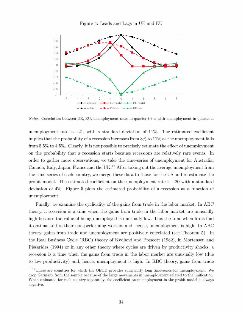
Figure 4: Leads and Lags in UE and EU

Notes: Correlation between UE, EU, unemployment rates in quarter t+ x with unemployment in quarter t.

unemployment rate is -.21, with a standard deviation of 11%. The estimated coeffi cient

implies that the probability of a recession increases from 8% to 11% as the unemployment falls

from 5.5% to 4.5%. Clearly, it is not possible to precisely estimate the effect of unemployment

on the probability that a recession starts because recessions are relatively rare events. In

order to gather more observations, we take the time-series of unemployment for Australia,

Canada, Italy, Japan, France and the UK.12 After taking out the average unemployment from

the time-series of each country, we merge these data to those for the US and re-estimate the

probit model. The estimated coeffi cient on the unemployment rate is -.20 with a standard

deviation of 4%. Figure 5 plots the estimated probability of a recession as a function of

unemployment.

Finally, we examine the cyclicality of the gains from trade in the labor market. In ABC

theory, a recession is a time when the gains from trade in the labor market are unusually

high because the value of being unemployed is unusually low. This the time when firms find

it optimal to fire their non-performing workers and, hence, unemployment is high. In ABC

theory, gains from trade and unemployment are positively correlated (see Theorem 5). In

the Real Business Cycle (RBC) theory of Kydland and Prescott (1982), in Mortensen and

Pissarides (1994) or in any other theory where cycles are driven by productivity shocks, a

recession is a time when the gains from trade in the labor market are unusually low (due

to low productivity) and, hence, unemployment is high. In RBC theory, gains from trade

12These are countries for which the OECD provides suffi ciently long time-series for unemployment. Wedrop Germany from the sample because of the large movements in unemployment related to the unification.When estimated for each country separately, the coeffi cient on unemployment in the probit model is alwaysnegative.

34

Figure 5: Probability of a Recession

Notes: Estimated probability of a recession next quarter as a function of current unemployment for US

(black solid line), UK (long-dashed blue line), Australia (short-dashed green line) and for a set of countries

pooled together (thick dashed line).

and unemployment are negatively correlated. To paint a picture, in ABC theory, a recession

is a time when the TV set is broken at home. In RBC theory, a recession is a time when

it is raining on the marketplace. Given the striking difference between these theories, it is

then natural to wonder whether the gains from trade in the labor market are indeed pro

or countercyclical. In order to address this question, we construct a rudimentary empirical

time-series of the workers’gains from trade, i.e. the difference between the value of being

employed and the value of being unemployed.13

We measure the value of employment to a worker, W1,t, and the value of unemployment

to a worker, W0,t, as

W1,t = wt + β[hEUt+1W0,t+1 + (1− hEUt+1)W1,t+1

],

W0,t = bt + β[hUEt+1W1,t+1 + (1− hUEt+1)W0,t+1

],

(26)

where wt is a measure of the real wage in month t, bt is a measure of unemployment ben-

efit/value of leisure in month t, hEUt+1 is a measure of the EU rate in month t + 1, hUEt+1 is a

measure of the UE rate in month t + 1, and W1,t+1 and W0,t+1 are respectively the value of

employment and unemployment in month t + 1. We measure the net value of employment

to a worker, Vt, in month t as the difference between W1,t and W0,t.

We measure wt using the time-series for the hourly wage that have been constructed by

Haefke, Sonntag and van Rens (2013). We consider two alternative time-series: the average

13We only attempt to measure the gains from trade accruing to the workers as measuring the gains fromtrade accruing to the firms requires the diffi cult task of constructing a time-series for profit per employee.When we try to measure profit per employee as labor productivity minus wages, we find that the firm’s gainsfrom trade are countercyclical as well.

35

hourly wage in the cross-section of all employed workers, and the average hourly wage in the

cross-section of newly hired workers after controlling for the composition of new hires. The

first time-series may be more appropriate when we want to interpret Vt as the cost of losing a

job to a worker, the second-time series may be more appropriate when we want to interpret

Vt as the benefit of finding a job to a worker. As in Shimer (2005), we measure hUEt and hEUtusing, respectively, the values for the EU rate and UE rates implied by the time-series for

unemployment and short-term unemployment. In order to make the time-series for wt, hUEtand hEUt stationary, we construct their Hodrick-Prescott trend using a smoothing parameter

of 105. We then take the difference between the value of each variable and its trend and add

this difference to the time-series average for that variable. Since bt is not directly observable,

we follow Hall and Milgrom (2008) and set it equal to 70% of the average of wt.

We are now in the position to construct time-series for the value of employment to a

worker, W1,t, and the value of unemployment to a worker, W0,t, over the period going from

January 1979 to December 2014. We compute the values for W1 and W0 in December 2014

by assuming that, from January 2015 onwards, w, hUE, and hEU are equal to their historical

averages. Given the values for W1 and W0 in December 2014, we compute the values for W1

and W0 from November 2014 back to January 1979 by using equation (26) and the time-

series for w, b, hUE, and hEU . The reader should notice that the values of W1 and W0 thus

computed differ from their theoretical counterpart because they are constructed using the

realizations of future w, hUE, and hEU , rather than the expectation of these variables.

Figure 6 presents the result of our calculations. Figure 6 displays the time-series for the

net value of employment to a worker, Vt, computed using the average wage of all employed

workers (solid black line) and the average wage of newly hired workers (dashed black line).

Figure 4 also displays the time-series for the detrended unemployment rate (solid grey line).

The figure clearly shows that Vt is countercyclical, in the sense that Vt moves together with

the unemployment rate. This is the case whether we measure Vt using the average wage

of all employed workers– in which the correlation between Vt and unemployment is 80%–

or whether we measure Vt using the average wage of newly hired workers– in which case

the correlation between Vt and unemployment is 71%. Mechanically, Vt is countercyclical

because, when unemployment increases, the decline in the value of being unemployed caused

by the large decline in the UE rate is larger than the decline in the value of being employed

cause by the small decline in the wage and by the short-lived increase in the EU rate. The

countercyclicality of Vt is a very robust finding. The measure of Vt becomes even more

countercyclical if bt is assumed to be constant fraction of wt rather than a constant. The

correlation between Vt and ut remains practically unchanged if we do not filter the data.

The finding that Vt is countercyclical means that recessions are times when unemployed

workers find it especially valuable to find a job, and when employed workers find it especially

36

Figure 6: Net Value of Employment

Notes: This figure reports the time series of unemployment (thick black solid line), the net value of em-

ployment computed using average wages (thick dashed blue line) and computed using the wage of new hires

(thin dashed red line).

costly to lose a job. The finding is in stark contrast with the view of recessions as “days of

rain in the marketplace” advanced by Kydland and Prescott (1982) or by Mortensen and

Pissarides (1994). In contrast, the finding is supportive of the view of recessions as “days

of no TV at home”advanced by our theory. Notice that our finding that Vt should not be

entirely surprising. Using a different, more sophisticated approach and richer data, Davis

and von Wachter (2011) show that the lifetime earning cost of losing a job is much higher

in recessions than in expansions. Even if one is skeptical about our theory of recessions, the

finding that Vt is countercyclical represents a challenge for many existing theories of business

cycles.

6 Conclusions

We developed a theory of endogenous and stochastic fluctuations in aggregate economic

activity. The structure of the theory is simple. Individual agents find it optimal to ran-

domize over some choice in order to overcome a non-convexity in their decision problem

and different agents across the economy find it optimal to correlate the outcome of their

randomization. Correlated randomization leads to aggregate fluctuations. These fluctua-

tions are endogenous– as they emerge from the agents’decision to randomize in a correlated

fashion– and they are stochastic– as they are the manifestation of a randomization process.

The unique feature of the theory is to generate a stochastic process for “shocks” that is

determined as an equilibrium outcome. We exemplified this theoretical structure with a

37

model where firms randomize over firing or keeping non-performing workers to provide them

with an incentive to exert effort and where different firms correlate the outcome of the ran-

domization to economize on the probability of firing. Other applications of the theoretical

structure seem promising. A particularly interesting application is to the credit market. As

in Clementi and Hopenhayn (2006), individual lenders may find it optimal to randomize

over continuing or terminating credit lines to firms that have performed poorly in the past.

Different lenders may find it optimal to correlate the outcome of their randomization in

order to minimize agency costs. In this context, correlated randomization might generate

endogenous and stochastic credit crunches.

References

[1] Agarwal, R., and J. Kolev. 2013 “Strategic Corporate Layoffs.”Manuscript, IMF.

[2] Angeletos, M., and J. La’O. 2013. “Sentiments.”Econometrica, 81: 739-780.

[3] Beaudry, P., D. Galizia, and F. Portier. 2016 “Reviving the Limit Cycle View of Macro-

economic Fluctuations,”NBER Working Paper 21241.

[4] Beaudry, P., and F. Portier. 2004. “Exploring Pigou’s Theory of Cycles.” Journal of

Monetary Economics, 51: 1183-1216.

[5] Benhabib, J., and R. Farmer. 1994. “Indeterminacy and Increasing Returns.”Journal

of Economic Theory, 63: 19—41.

[6] Bloom, N. 2009. “The Impact of Uncertainty Shocks.”Econometrica, 77: 623-685.

[7] Boldrin, M., and L. Montrucchio. 1986. “On the Indeterminacy of Capital Accumulation

Paths.”Journal of Economic Theory, 40: 26-39.

[8] Boldrin, M., and M. Woodford. 1990. “Equilibrium Models Displaying Endogenous

Fluctuations and Chaos.”Journal of Monetary Economics, 25: 189-222.

[9] Cappelli, P., and K. Chauvin. 1991. “An Interplant Test of the Effi ciency Wage Hy-

pothesis.”Quarterly Journal of Economics, 106: 769-787

[10] Chodorow-Reich, G., and L. Karabarbounis. 2016. “The Cyclicality of the Opportunity

Cost of Employment.”Forthcoming, Journal of Political Economy.

[11] Clementi, G., and H. Hopenhayn. 2006. “A Theory of Financing Constraints and Firm

Dynamics.”Quarterly Journal of Economics, 121: 229-65.

38

[12] Cooper, R., and A. John. 1988. “Coordinating Coordination Failures in Keynesian Mod-

els.”Quarterly Journal of Economics, 103: 441—63.

[13] Corgnet, B., R. Hernán-Gonzales, and S. Rassenti. 2015. “Firing Threats: Incentive

Effects and Impression Management.”Games and Economic Behavior 91: 97-113.

[14] Davis, S., and T. von Wachter. 2011. “Recessions and the Costs of Job Loss.”Brookings

Papers on Economic Activity.

[15] Diamond, P. 1982. “Aggregate Demand Management in Search Equilibrium.”Journal

of Political Economy, 90: 881—94.

[16] Diamond, P., and D. Fudenberg. 1989. “Rational Expectations Business Cycles in Search

Equilibrium.”Journal of Political Economy, 97: 606—19.

[17] Farmer, R. 2013 “Animal Spirits, Financial Crises and Persistent Unemployment”, Eco-

nomic Journal, 123: 317-340.

[18] Fujita, S., and G. Ramey. 2009. “The Cyclicality of Separation and Job Finding Rates.”

International Economic Review, 50: 415—30.

[19] Gabaix, X. 2011. “The Granular Origins of Aggregate Fluctuations.”Econometrica 79:

733-772.

[20] Galí, J., and T. van Rens. 2014. “The Vanishing Procyclicality of Labor Productivity.”

Manuscript, University of Warwick.

[21] Gertler, M., and A. Trigari. 2009. “Unemployment Dynamics with Staggered NashWage

Bargaining.”Journal of Political Economy, 117: 38-86.

[22] Haefke, C., M. Sonntag, and T. van Rens, 2013. “Wage Rigidity and Job Creation.”

Journal of Monetary Economics.

[23] Hagedorn, M., and I. Manovskii. 2008. “The Cyclical Behavior of Unemployment and

Vacancies Revisited.”American Economic Review, 98: 1692—706.

[24] Hall, R., 2005. “Employment Fluctuations with Equilibrium Wage Stickiness.”Ameri-

can Economic Review, 95: 50-65.

[25] Hall, R. 2016. “High Discounts and High Unemployment,”American Economic Review,

Forthcoming.

[26] Hall, R., and P. Milgrom. 2008. “The Limited Influence of Unemployment of the Wage

Bargain.”American Economic Review, 98: 1653—74.

39

[27] Heller, W. 1986. “Coordination Failure Under Complete Markets with Applications to

Effective Demand.” Equilibrium analysis: Essays in Honor of Kenneth J. Arrow, 2:

155—175.

[28] Ichino, A., and R. Riphahn. 2005. “The Effect of Employment Protection on Worker

Effort: Absenteeism during and after Probation.” Journal of the European Economic

Association, 3: 120-143.

[29] Jaimovich, N., and S. Rebelo. 2009. “Can News About the Future Drive Business Cy-

cles?”American Economic Review, 99: 1097-1118.

[30] Jenter, D., and F. Kanaan. 2015. “CEO Turnover and Relative Performance Evalua-

tion.”Journal of Finance 50: 2155-2183.

[31] Jovanovic, B. 1987. “Micro Shocks and Aggregate Risk.”Quarterly Journal of Eco-

nomics, 102: 395-409.

[32] Kaplan, G., and G. Menzio. 2016. “Shopping Externalities and Self-Fulfilling Unem-

ployment Fluctuations.”Journal of Political Economy, 124: 771-825.

[33] Kennan, J. 2010. “Private Information, Wage Bargaining and Employment Fluctua-

tions.”Review of Economic Studies, 77: 633-64.

[34] Kydland, F., and E. Prescott. 1982. “Time to Build and Aggregate Fluctuations.”

Econometrica, 50: 1345-70.

[35] Menzio, G. 2005. “High Frequency Wage Rigidity.”Manuscript, Northwestern Univer-

sity.

[36] Menzio, G., and E. Moen. 2010. “Worker Replacement.” Journal of Monetary Eco-

nomics, 57: 623-36.

[37] Menzio, G., and S. Shi. 2010. “Block Recursive Equilibria for Stochastic Models of

Search on the Job.”Journal of Economic Theory, 145: 1453-94.

[38] Menzio, G., and S. Shi. 2011. “Effi cient Search on the Job and the Business Cycle.”

Journal of Political Economy, 119: 468—510.

[39] Mortensen, D. 1999. “Equilibrium Unemployment Dynamics.”International Economic

Review, 40: 889—914.

[40] Mortensen, D., and C. Pissarides. 1994. “Job Creation and Job Destruction in the

Theory of Unemployment.”Review of Economic Studies, 61: 397—415.

40

[41] Petrongolo, B., and C. Pissarides. 2001. “Looking into the Black Box: A Survey of the

Matching Function.”Journal of Economic Literature, 39: 390-431.

[42] Pissarides, C. 1985. “Short-Run Equilibrium Dynamics of Unemployment, Vacancies

and Real Wages.”American Economic Review, 75: 676—90.

[43] Shapiro, C, and J. Stiglitz. 1984. “Equilibrium unemployment as a worker discipline

device.”American Economic Review, 74: 433-443.

[44] Shimer, R. 2005. “The Cyclical Behavior of Unemployment and Vacancies.”American

Economic Review, 95: 25—49.

[45] Stokey, N., R. Lucas, and E. Prescott, “Recursive Methods in Economic Dynamics.”

Harvard University Press, Cambridge, Massachusetts, 1989.

41

Online Appendix

A Proof of Lemmas 1-4

A.1 Proof of Lemma 1

Let ρ ≥ 0 denote the Lagrange multiplier on the worker’s incentive compatibility constraint,

let ν(y, z) ≥ 0 denote the multiplier on the constraint 1− s(y, z) ≥ 0 and let ν(y, z) denote

the multiplier on the constraint s(y, z) ≥ 0.

The first order condition with respect to the firing probability s(y`, z) is given by

(1− δ) [F (x)V (z) +W (x)J(z)] = ρβ(1− δ)(ph(1)− ph(0))V (z) + ν(y`, z)− ν(y`, z), (A1)

together with the complementary slackness conditions ν(y`, z) ·(1−s(y`, z)) = 0 and ν(y`, z) ·s(y`, z) = 0. The left-hand side of (A1) is the marginal cost of increasing s(y`, z). This cost

is given by the decline in the product of the worker’s and firm’s gains from trade caused

by a marginal increase in the firing probability s(y`, z). The right-hand side of (A1) is the

marginal benefit of increasing s(y`, z). This benefit is given by the value of relaxing the

worker’s incentive compatibility and the s(y`, z) ≥ 0 constraints net of the cost of tightening

the s(y`, z) ≤ 1 constraint by marginally increasing the firing probability s(y`, z).

Similarly, the first order condition with respect to the firing probability s(yh, z) is given

by

(1− δ) [F (x)V (z) +W (x)J(z) + ρβ(ph(1)− ph(0))V (z)] = ν(yh, z)− ν(yh, z), (A2)

together with the complementary slackness conditions ν(yh, z)·(1−s(yh, z)) = 0 and ν(yh, z)·s(yh, z) = 0. The left-hand side of (A2) represents the marginal cost of increasing s(yh, z).

The rigth-hand side of (A2) represents the marginal benefit of increasing s(yh, z). Notice

that increasing the firing probability s(yh, z) tightens the worker’s incentive compatibility

constraint and, hence, the term in ρ is now on the left-hand side of (A2).

Suppose ρ = 0. First, notice that the left-hand side of (A1) is strictly positive as V (z) > 0,

J(z) > 0 by assumption, and W (x) > 0, F (x) > 0 at the optimum x∗. The right-hand side

of (A1) is strictly positive only if ν(y`, z) > 0. Hence, if ρ = 0, the only solution to the

first order condition with respect to the firing probability s(y`, z) is 0. Next, notice that

the left-hand side of (A2) is strictly positive and the right-hand side is strictly positive

only if ν(yh, z) > 0. Hence, if ρ = 0, the only solution to the first order condition with

respect to the firing probability s(yh, z) is 0. However, if s(y`, z) = s(yh, z) = 0, the worker’s

incentive compatibility constraint is violated. Therefore, ρ > 0 and the worker’s incentive

compatibility constraint holds with equality.

42

A.2 Proof of Lemma 2

The first order condition with respect to s(yh, z) is given by (A2) together with the com-

plementary slackness conditions ν(yh, z)(1 − s(yh, z)) = 0 and ν(yh, z)s(yh, z) = 0. The

left-hand side of (A2) is strictly positive. The right-hand side of (A2) is strictly positive

only if ν(yh, z) > 0. Therefore, the first order condition is satisfied only if ν(yh, z) > 0 and,

hence, only if s(yh, z) = 0.

A.3 Proof of Lemma 3

Using the definition of φ(z), we can rewrite the first order condition with respect to the firing

probability s(y`, z) as

(1− δ)V (z) [F (x) +W (x)/φ(z)− ρβ(ph(1)− ph(0))] = ν(y`, z)− ν(y`, z), (A3)

together with ν(y`, z) · (1 − s(y`, z)) = 0 and ν(y`, z) · s(y`, z) = 0. The left-hand side of

(A3) is strictly decreasing in φ(z). The right-hand side of (A3) is strictly positive if ν(y`, z)

is strictly positive and it is strictly negative if ν(y`, z) is strictly positive. Therefore, there

exists a φ∗ such that if φ(z) > φ∗, the left-hand side is strictly negative and the solution to

(A3) requires ν(y`, z) > 0. In this case, the solution to the first order condition for s(y`, z)

is 1. If φ(z) < φ∗, the left-hand side is strictly positive and the solution to (A3) requires

ν(y`, z) > 0. In this case, the solution to the first order condition for s(y`, z) is 0.

A.4 Proof of Lemma 4

The first order condition with respect to the wage w is given by

F (x)υ′(w)−W (x) = 0. (A4)

The left-hand side of (A4) is the increase in the product of the worker’s and firm’s gains

caused by a marginal increase in the worker’s wage w. A marginal increase in w, increases the

worker’s gains from trade by υ′(w) and decreases the firm’s gains from trade by 1. Therefore,

a marginal increase in w, increases the product of the worker’s and firm’s gains from trade

by F (x)υ′(w) −W (x). The first order condition for w states that the effect of a marginal

increase in w is zero.

B Proof of Lemmas 5-6

B.1 Proof of Lemma 5

We first consider a firm-worker pair in group K. Since PK(TK |TK−1) is strictly increasing inTK−1 and u is strictly increasing in TK , E[u|TK−1] is strictly increasing in TK−1. In turn, since

43

E[u|TK−1] is strictly increasing in TK−1 and φ(u) is strictly increasing in u, φ(E[u|TK−1]) isstrictly increasing in TK−1. It then follows from property (iii) of the optimal contract that

there exists a T ∗K−1 such that sK(y`, TK−1) = 0 for all TK−1 < T ∗K−1, and sK(y`, TK−1) = 1

for all TK−1 > T ∗K−1. This establishes that the firing probability sK(y`, TK−1) has the desired

threshold property. The threshold property implies that the measure tK of workers separating

from firms in group K is increasing in the measure TK−1 of workers separating from firms in

groups 1 through K − 1.

Next, consider a firm-worker pair in group K − 1. Since PK−1(TK−1|TK−2) is strictlyincreasing in TK−2 and tK is increasing in TK−1, it follows that E[u|TK−2] and, in turn,φ(E[u|TK−2]) are strictly increasing in TK−2. Then property (iii) of the optimal contractimplies that there exists a T ∗K−2 such that sK−1(y`, TK−2) = 0 for all TK−2 < T ∗K−2, and

sK−1(y`, TK−2) = 1 for all TK−2 > T ∗K−2. This establishes that the firing probability

sK−1(y`, TK−2) has the desired threshold property. The threshold property implies that the

measure tK−1 of workers separating from firms in group K − 1 is increasing in the measure

TK−2 of workers separating from firms in groups 1 through K − 2. By repeating the above

argument for firm-worker pairs in groups K − i, with i = 2, 3, . . . K − 1, we can establish

that the firing probability sK−i(y`, TK−i−1) has the threshold property and that the measure

tK−i is increasing in TK−i−1.

B.2 Proof of Lemma 6

Let T ∗1 be given as in (22) and let T∗i = E[t1]+(i−1)(th− t`)/2 for i = 2, 3, . . . K−1. Given

the thresholds T ∗1 , T ∗2 , ...T ∗K−1, we can compute the unconditional probability distributionof the random variable Ti. ForN →∞, T2 is approximately equal to E[t1]+t` if T1 < T ∗1 , and

it is approximately equal to E[t1]+th if T1 > T ∗1 . Since E[t1]+t` < T ∗2 and E[t1]+th > T ∗2 , T3is approximately equal to E[t1] + 2t` if T1 < T ∗1 , and T3 is approximately equal to E[t1] + 2th

if T1 > T ∗1 . Similarly, for i = 4, 5, . . . K, Ti is approximately equal to E[t1] + (i − 1)t` if

T1 < T ∗1 , and it is approximately equal to E[t1] + (i − 1)th if T1 > T ∗1 . Hence, if T1 < T ∗1 ,

firms in groups 2 through K fire their non-performing workers with probability 0 and the

total measure of workers separating from firms is TK = E[t1] + (K − 1)t`. If T1 > T ∗1 , firms

in groups 2 through K fire their non-performing workers with probability 1 and the total

measure of workers separating from firms is Tk = E[t1] + (K − 1)th.

The above observations imply that benefit from exerting effort for a worker employed at

a firm in group i = 2, 3, . . . K is given by

β(1− δ)(ph(1)− ph(0))(1− P1(T ∗1 ))V (E[u|TK = E[t1] + (K − 1)th]). (B1)

The benefit in (B1) is equal to the cost ψ of exerting effort given the choice of T ∗1 . Thus, the

incentive compatibility for workers employed by firms in groups i = 2, 3, . . . K is satisfied.

44

The incentive compatibility constraint for workers employed by firms in group 1 is satisfied

given the choice of s1.

C Proof of Theorem 4

The existence proof is based on an application of Schauder’s fixed point theorem. In partic-

ular, we are going to take arbitrary value functions V +(u) and J+(u) denoting, respectively,

the worker’s gains from trade at the end of the production stage and the firm’s gains from

trade at the end of the production stage. Then, we are going to use the conditions for a Re-

cursive Equilibrium with perfect correlation to construct a mapping F that returns updatesfor V +(u) and J+(u). Using Schauder’s fixed point theorem, we are going to prove that the

mapping F admits a fixed point and we are going to show that this fixed point is a RecursiveEquilibrium with perfect correlation in the stage game.

The functions V +(u) and J+(u) are chosen from a set Ω of Lipschitz continuous functions

with fixed Lipschitz bounds. These property of the set Ω is critical to establish that the

operator F satisfies the conditions for Schauder’s fixed point theorem (namely, that the

family of functions F(⊗) is equicontinuous). Formally, let Ω denote the set of bounded and

continuous functions ω(u, i) = iV +(u) + (1− i)J+(u), with ω : [0, 1]× 0, 1 → R, and suchthat: (i) for all u0, u1 ∈ [0, 1] with u0 < u1, V +(u1)−V +(u0) is greater thanDV+(u1−u0) andsmaller than DV+(u1−u0); (ii) for all u0, u1 ∈ [0, 1] with u0 < u1, J+(u1)−J+(u0) is greater

than DJ+(u1 − u0) and smaller than DJ+(u1 − u0). In other words, Ω is the set of bounded

and Lipschitz continuous functions ω = (V +, J+) with fixed Lipschitz bounds DV+ , DV+,

DJ+ and DJ+. We choose the Lipschitz bounds to satisfy DV+ > DV+ > 0, DJ+ > 0 ≥ DJ+,

and DV+ > υ′(DJ+ −DJ+).

Starting from V +(u) and J+(u) in Ω, we use the equilibrium conditions to construct the

equilibrium wage, the equilibrium gains from trade accruing to the worker and the firm, the

equilibrium law of motion for unemployment and an update for V +(u) and J+(u). This

process implicitely defines the operator F . In order to make sure that F maps functions inΩ into functions in Ω (which is a condition of Schauder’s fixed point theorem), we need to

verify that all equilibrium objects are Lipschitz continuous with fixed Lipschitz bounds. In

order to make sure that F is continuous (which is also a condition of Schauder’s fixed pointtheorem), we need to verify that all equilibrium objects are continuous. To carry out these

tasks, we need a few more pieces of notation. In particular, we use V , V , J and J to denote

lower and upper bounds on the worker’s and firm’s gains from trade constructed as in (??).Also, we use µu and µu to denote the minimum and the maximum of the (absolute value) of

the partial derivative of the job-finding probability µ(J, u) with respect to i = u. That is,

µu denotes min |∂µ(J, u)/∂u| for (J, u) ∈ [J, J ]× [0, 1], and µu denotes max |∂µ(J, u)/∂u| for

45

(J, u) ∈ [J, J ]× [0, 1]. Similarly, we use µJ and µJ to denote the minimum and the maximum

on the (absolute value) of the partial derivative of µ(J, u) with respect to J .

C.1 Wage

Take an arbitrary pair of value functions ω = (V +, J+) ∈ Ω. For any u, the equilibrium

wage function w(u) takes a value w such that

υ(w)− υ(b)− ψ + V +(u) = υ′(w)[E[y|e = 1]− w + J+(u)

]. (C1)

For any u, there is a unique wage that satisfies (C1). In fact, the right-hand side of (C1) is

strictly increasing in w, as υ(w)−υ(b)−ψ+V +(u) is strictly increasing in w. The left-hand

side of (C1) strictly decreasing in w, as υ′(w) and E[y|e = 1]− w + J+(u) are both strictly

decreasing in w. Therefore, there exists a unique wage w that solves (C1) for any u.

The next lemma proves that the equilibrium wage function w(u) is Lipschitz continuous

in u with fixed Lipschitz bounds. Moreover, the lemma proves that w(u) is strictly decreasing

in u.

Lemma C1: For all u0, u1 ∈ [0, 1] with u0 < u1, the wage function w(u) is such that

Dw(u1 − u0) ≤ w(u0)− w(u1) ≤ Dw(u1 − u0), (C2)

where the bounds Dw and Dw are defined as

Dw =DV+/υ

′ −DJ+

2 + Jυ′′/υ′, Dw = DV+/υ

′ −DJ+. (C3)

Proof : To alleviate notation, let w0 denote w(u0) and w1 denote w(u1). First, we establish

that w0 > w1. To this aim, notice that

υ′(w0) [E[y|e = 1]− w0 + J+(u1)]

≤ υ′(w0)E[y|e = 1]− w0 + J+(u0)] + υ′DJ+(u1 − u0).(C4)

Also, notice that

υ(w0)− υ(b)− c+ V +(u1)

≥ υ(w0)− υ(b)− c+ V +(u0) +DV+(u1 − u0)= υ′(w0)E[y|e = 1]− w0 + J+(u0) +DV+(u1 − u0)> υ′(w0)E[y|e = 1]− w0 + J+(u0) + υ′DJ+(u1 − u0),

(C5)

where the third line follows from (C1) and the last line follows from DV+ > υ′DJ+. Taken

together (C4) and (C5) imply that υ(w0) − υ(b) − c + V +(u1) is strictly greater than

υ′(w0) [E[y|e = 1]− w0 + J+(u1)]. Therefore, the left-hand side of (C1) is strictly smaller

46

than the right-hand side of (C1) when evaluated at w = w0 and u = u1. Since the left-hand

of (C1) is strictly increasing in w and the left-hand side is strictly decreasing in w, w1 is

strictly smaller than w0.

Next, we derive lower and upper bounds on w0 − w1. From (C1), it follows that

υ(w0)− υ(w1) + V +(u0)− V +(u1)

= υ′(w0) [E[y|e = 1]− w0 + J+(u0)]− υ′(w1) [E[y|e = 1]− w0 + J+(u0)]

+ υ′(w1) [E[y|e = 1]− w0 + J+(u0)]− υ′(w1) [E[y|e = 1]− w1 + J+(u1)]

(C6)

The above equation can be rewritten as

w0 − w1

=

[V +(u1)− V +(u0)

υ′(w1)

]− [J+(u1)− J+(u0)]

−[υ(w0)− υ(w1)

υ′(w1)

]−[υ′(w1)− υ′(w0)

υ′(w1)(E[y|e = 1]− w0 + J+(u0))

].

(C7)

The first term in square brackets on the right-hand side of (C6) is greater than (DV+/υ′)(u1−

u0) and smaller than (DV+/υ′)(u1−u0). The second term in square brackets is greater than

DJ+(u1 − u0) and smaller than DJ+(u1 − u0). The third term in square brackets is greater

than zero and smaller than w1−w0. The last term on the right-hand side of (C6) is greater

than zero and smaller than υ′′DwJ/υ′(w1−w0). From the above observations, it follows that

w0 − w1 ≤[DV+

υ′−DJ+

](u1 − u0). (C8)

Similarly, we have

w0 − w1 ≥[2 +

υ′′

υ′DwJ

]−1 [DV+

υ′−DJ+

](u1 − u0). (C9)

The inequalities (C8) and (C9) represent the desired bounds on w0 − w1. The next lemma proves that the equilibrium wage function w is continuous with respect

to the value functions V + and J+. Specifically, consider ω0 = (V +0 , J

+0 ) and ω1 = (V +

1 , J+1 )

with ω0, ω1 ∈ Ω. Denote as wi the wage function computed using ωi in (C1) for i = 0, 1.If the distance between ω0 and ω1 goes to 0, so does the distance between w0 and w1.

Lemma C2: For any κ > 0 and any ω0, ω1 in Ω such that ||ω0- ω1|| < κ, we have

||w0 − w1|| < αwκ, αw = 1 + 1/υ′. (C10)

Proof : Take an arbitrary u ∈ [0, 1]. To alleviate notation, let w0 denote w0(u) and w1

denote w1(u). From (C10), it follows that

υ(w0)− υ(b)− c+ V +0 (u)− υ′(w0)

[E[y|e = 1]− w0 + J+0 (u)

]= 0,

υ(w1)− υ(b)− c+ V +1 (u)− υ′(w1)

[E[y|e = 1]− w1 + J+1 (u)

]= 0.

(C11)

47

Subtracting the second equation from the first, we obtain

V +0 (u)− V +

1 (u) + υ(w0)− υ(w1)

+ υ′(w0)[J+1 (u)− J+0 (u) + w0 − w1

]+ [υ′(w1)− υ′(w0)]

[E[y|e = 1]− w1 + J+1 (u)

]= 0.

(C12)

Suppose without loss in generality that w0 ≥ w1. We can rewrite the above equation as

w0 − w1 =[J+0 (u)− J+1 (u)

]+

[V +1 (u)− V +

0 (u)

υ′(w0)

]+

[υ(w1)− υ(w0)

υ′(w0)

]+[E[y|e = 1]− w1 + J+1 (u)

] [υ′(w0)− υ′(w1)υ′(w0)

].

(C13)

The first term in square brackets on the right-hand side of (C13) is strictly smaller than κ.

The second term in square brackets is strictly smaller than κ/υ′. The third term in square

brackets is strictly negative. The last term is strictly negative. Hence, we have

0 ≤ w0 − w1 < (1 + 1/υ′)κ. (C14)

Since the above inequality holds for any u ∈ [0, 1], we conclude that ‖w0 − w1‖ < αwκ where

αw = (1 + 1/υ′).

C.2 Gains from trade to worker and firm

Given V +, J+ and w, the equilibrium gains from trade accruing to the firm and to the

worker, J and V , are respectively given by

J(u) = E[y|e = 1]− w(u) + J+(u),

V (u) = υ(w(u))− υ(b)− ψ + V +(u)(C15)

The next lemma proves that the equilibrium gains from trade J(u) and V (u) are Lipschitz

continuous in u with fixed Lipschitz bounds. Moreover, the lemma proves that J(u) and V (u)

are strictly increasing in u.

Lemma C3: For all u0, u1 ∈ [0, 1] with u0 < u1, the equilibrium gains from trade accruing

to the firm, J(u), and to the worker, V (u), are such that

DJ(u1 − u0) ≤ J(u1)− J(u0) ≤ DJ(u1 − u0),DV (u1 − u0) ≤ V (u1)− V (u0) ≤ DV (u1 − u0),

(C16)

where the bounds are defined as

DJ = Dw +DJ+ > 0, DJ = Dw +DJ+ ,

DV = υ′(Dw +DJ+) > 0, DV = υ′(Dw +DJ+) + υ′′DwJ.(C17)

Proof : To simplify notation, let w0 denote w(u0) and w1 denote w(u1). Then J(u1)−J(u0)

48

is given by

J(u1)− J(u0) = w0 − w1 + J+(u1)− J+(u0).

From the above expression, it follows that

J(u1)− J(u0) ≥ (Dw +DJ+)(u1 − u0),J(u1)− J(u0) ≤ (Dw +DJ+)(u1 − u0).

(C18)

The difference V (u1)− V (u0) is given by

V (u1)− V (u0) = υ′(w1)J(u1)− υ′(w0)J(u0)

= [υ′(w1)J(u1)− υ′(w1)J(u0)] + [υ′(w1)J(u0)− υ′(w0)J(u0)]

From the above expression, it follows that

V (u1)− V (u0) ≥ υ′(Dw +DJ+)(u1 − u0),V (u1)− V (u0) ≤

[υ′(Dw +DJ+) + υ′′DwJ

](u1 − u0).

(C19)

Lemma 7 follows directly from the inequalities in (C18) and (C19). The next lemma proves that the firm’s and worker’s gains from trade are continuous with

respect to V + and J+. Specifically, consider ω0 = (V +0 , J

+0 ) and ω1 = (V +

1 , J+1 ) with ω0,

ω1 in Ω. For i ∈ 0, 1, denote as wi the equilibrium wage computed using ωi, and as Jiand Vi the equilibrium gains from trade computed using ωi and wi in (C15). If the distance

between ω0 and ω1 goes to 0, so does the distance between J0 and J1 and between V0 and

V1.

Lemma C4: For any κ > 0 and any ω0, ω1 in Ω such that ||ω0- ω1|| < κ, we have

||J0 − J1|| < αJκ, αJ = 1 + αw,

||V0 − V1|| < αV κ, αV = 1 + υ′αw.. (C20)

Proof : Take an arbitrary u ∈ [0, 1]. The difference J0(u)− J1(u) is such that

|J0(u)− J1(u)| ≤ |w0(u)− w1(u)|+∣∣J+0 (u)− J+1 (u)

∣∣< (αw + 1)κ.

(C21)

The difference V0(u)− V1(u) is such that

|V0(u)− V1(u)| ≤ |υ(w0(u))− υ(w1(u))|+∣∣V +0 (u)− V +

1 (u)∣∣

< (υ′αw + 1)κ.(C22)

Since the inequalities (C21) and (C22) hold for all u ∈ [0, 1], we conclude that ‖J0 − J1‖ <αJ ′κ and ‖V0 − V1‖ < αV ′κ, where αJ = αw + 1 and αV = υ′αw + 1.

49

C.3 Law of motion for unemployment

Given J , the law of motion for unemployment h(u, z), is such that– for any current period’s

unemployment u and any realization of the sunspot z– next period’s unemployment takes

on a value u such that

u = u− uµ(J(u), u) + (1− u)[δ + (1− δ)p`(1)s(y`, z)], (28)

Since we are trying to construct a Recursive Equilibrium in which there is perfect correlation

in the stage game, we set s(y`, z) = 0 if z ∈ Z0 and s(y`, z) = 1 if z ∈ Z2.Next period’s unemployment u is uniquely determined by (28). In fact, the left-hand

side of (28) equals zero for u = 0, it is strictly increasing in u and it equals one for u = 1.

The right-hand side of (28) is strictly positive for u = 0 and it is strictly decreasing in u,

as the worker’s job finding probability µ is strictly increasing in the firm’s gains from trade

J , and J is strictly increasing in u. Therefore, there exists one and only one u that satisfies

(28). Next period’s unemployment u is strictly increasing in u. In fact, the left-hand side

of (28) is independent of u. The right-hand side of (28) is strictly increasing in u, as its

derivative with respect to u is greater than (1− δ)ph(1)− µ, which we assume to be strictlypositive. Therefore, the u that solves (28) is strictly increasing in u. Moreover, next period’s

unemployment u is strictly higher if z ∈ Z2 than if z ∈ Z0. To see this, it is suffi cient to

notice that the left-hand side of (28) is independent of s(y`, z), while the right hand side is

strictly increasing in it.

The next lemma proves that h(u, z) is Lipschitz continuous in u with fixed Lipschitz

bounds.

Lemma C5: For all u0, u1 ∈ [0, 1] with u0 < u1, h(u, z) is such that

Dh(u1 − u0) < h(u1, z)− h(u0, z) ≤ Dh(u1 − u0), (C24)

where the bounds Dh and Dh are defined as

Dh = 0, Dh = 1− δ + µu. (C25)

Proof : Let u1 denote the solution to (28) for u = u1 and let u0 denote the solution to (28)

for u = u0, i.e.

u1 = u1 − u1µ(J(u1), u1) + (1− u1)[δ + (1− δ)p`(1)s(y`, z′)],

u0 = u0 − u0µ(J(u0), u0) + (1− u0)[δ + (1− δ)p`(1)s(y`, z′)].

Subtracting the second equation from the first one, we obtain

u1 − u0 = (u1 − u0)(1− δ)[1− p`(1)s(y`, z′)]

+u0 [µ (J(u0), u0)− µ (J(u1), u0)]

+u0 [µ (J(u1), u0)− µ (J(u1), u1)]

+u0µ (J(u1), u1)− u1µ (J(u1), u1) .

(C26)

50

The first line on the right-hand side of (C26) is positive. Since µ(J, u) is increasing in J ,

J is increasing in u and, as established in the main text, u1 > u0, the second line on the

right-hand side of (C26) is negative. Since µ(J, u) is decreasing in u and u1 > u0, the third

line on the right-hand side of (C26) is positive. The fourth line on the right-hand side of

(C26) is obviously negative. Hence, an upper bound on u1 − u0 is given by

u1 − u0 ≤ (u1 − u0)(1− δ)[1− p`(1)s(y`, z′)] + u0 [µ (J(u1), u0)− µ (J(u1), u1)]

≤ (u1 − u0) [1− δ + µu] .(C27)

Combining the above inequality with u1 < u0, we obtain

Dh (u1 − u0) < u1 − u0 ≤ Dh (u1 − u0) , (C28)

where

Dh = 0, Dh = 1− δ + µu.

Next, we prove that h(u, z) is continuous with respect to V + and J+. Formally, we

consider ω0 = (V +0 , J

+0 ) and ω1 = (V +

1 , J+1 ) with ω0, ω1 in Ω. For i = 0, 1, we denote

as Ji the firm’s equilibrium gains from trade computed using ωi in (C15), and as hi the

equilibrium law of motion for unemployment computed using Ji in (28). Then, we show

that, if the distance between ω0 and ω1 goes to 0, so does the distance between h0 and h1.

Lemma C6: For any κ > 0 and any ω0, ω1 in Ω such that ||ω0- ω1|| < κ, we have

||h0 − h1|| < αhκ, αh = µJαJ . (C29)

Proof : Take an arbitrary u ∈ [0, 1] and z ∈ Z0, Z2. Let u0 denote h0(u, z) and u1 denote

h1(u, z). From (28), it follows that

u0 = u− uµ(J0(u0), u) + (1− u)[δ + (1− δ)p`(1)s(y`, z)],

u1 = u− uµ(J1(u1), u) + (1− u)[δ + (1− δ)p`(1)s(y`, z)].

Without loss in generality suppose that u0 ≥ u1. In this case,

u0 − u1 = u [µ(J1(u1), u)− µ(J0(u1), u)] + [µ(J0(u1), u)− µ(J0(u0), u)] . (C30)

The term µ(J0(u1), u)− µ(J0(u0), u) on the right-hand side of (C30) is negative as µ(J, u) is

increasing in J , J0 is increasing in u and u0 ≥ u1. Therefore, we have

u0 − u1 ≤ u [µ(J1(u1), u)− µ(J0(u1), u)] < µJαJκ. (C31)

Since the above inequality holds for any u ∈ [0, 1] and any z′ ∈ B,G, we conclude that‖h0 − h1‖ < αhκ, where αh = µJαJ .

51

C.4 Updated value functions

Given J , V and h, we can construct an update, V +′, for the worker’s gains from trade at

the end of the production stage as

V +′(u) = βEz [(1− δ)(1− p`(1)s(y`, z))− µ(J(h(u, z)), u)]V (h(u, z)) (C32)

Similarly, we can construct an update, J+′, for the firm’s gains from trade at the end of the

production stage as

J+′(u) = βEz [(1− δ)(1− p`(1)s(y`, z))J(h(u, z))] (C33)

Since we are looking for a Recursive Equilibrium with perfect correlation in the stage game,

we set s(y`, z) = 0 for z ∈ Z0 and s(y`, z) = 1 for z ∈ Z2. Also, we set the probability π0that z ∈ Z0 and the probability π2 that z ∈ Z2 so that π0 = 1− π2 and

π2 =ψ

β(ph(1)− ph(0))(1− δ)V (h(u, Z2)). (C34)

In the next lemma, we prove that V +′(u) and J+′(u) are Lipschitz continuous in u with

fixed Lipschitz bounds.

Lemma C7: For all u0, u1 ∈ [0, 1] with u0 < u1, V +′ and J+′ are such that

D′V+(u1 − u0) < V +′(u1)− V +′(u0) ≤ D′V+(u1 − u0),

D′J+(u1 − u0) < J+′(u1)− J+′(u0) ≤ D′J+(u1 − u0).

(C35)

where the bounds D′V+ and D′V+ are defined as

D′V+ = βV (µu− µJDJDh)−

2ψDVDhV

(ph(1)− ph(0))(1− δ)V 2 ,

D′V+ = β

[V µu + (1− δ)DVDh

],

(C36)

and the bounds D′J+ and D′J+ are defined as

D′J+ = − 2cDVDhJ

(ph(1)− ph(0))(1− δ)V 2 ,

D′J+ = β(1− δ)DJDh

(C37)

Proof : Take arbitrary u0, u1 ∈ [0, 1] with u1 > u0. To simplify notation, let uj,0 denote

h(u0, z) for z ∈ Zj and let uj,1 denote h(u1, z) for z ∈ Zj. Similarly, let πj,0 denote the

probability that the realization of the sunspot is z ∈ Zj for u0, and let πj,1 denote the

52

probability that the realization of the sunspot is z ∈ Zj for u1. Using this notation and

(C32), we can write V +′(u1)− V +′(u0) as

V +′(u1)− V +′(u0)

= β∑

j (πj,1 − πj,0) [(1− δ)(1− p`(1)s(y`, z))− µ(J(uj,1, u1)]V (uj,1)

+ πj,0[(1− δ)(1− p`(1)s(y`, z))− µ(J(u2,1, u1)] [V (uj,1)− V (uj,0)]

+ πj,0V (uj,0)[µ(J(u2,0, u0)− µ(J(u2,0, u1)].

+ πj,0V (uj,0)[µ(J(u2,0, u1)− µ(J(u2,1, u1)].

(C38)

The first term on the right-hand side of (C38) is negative. In absolute value, this term is

smaller than cDVDhV (u1 − u0)/[β(ph(1)− ph(0))(1− δ)V 2]. The second term on the right-

hand side of (C38) is geater than 0 and smaller than πj,0(1 − δ)DVDh(u1 − u0). The thirdterm on the right-hand side of (C38) is positive, greater than πj,0V µu(u1 − u0) and smallerthan πj,0V µu(u1−u0). The last term on the right-hand side of (C38) is negative. In absolutevalue, this term is smaller than πj,0V µJDJDh(u1 − u0). Overall, we have

V +′(u1)− V +′(u0) ≥[βV (µ

u− µJDJDh)−

2cDVDhV

(ph(1)− ph(0))(1− δ)V 2

](u1 − u0), (C39)

and

V +′(u1)− V +′(u0) ≤ β[V µu + (1− δ)DVDh

](u1 − u0). (C40)

Using (C33), we can write J+′(u1)− J+′(u0) as

J+′(u1)− J+′(u0)= β

∑j (πj,1 − πj,0) [(1− δ)(1− p`(1)s(y`, z))]J(uj,1)

+ πj,0[(1− δ)(1− p`(1)s(y`, z))] [J(uj,1)− J(uj,0)] .

(C41)

The first term on the right-hand side of (C41) is negative. In absolute value, this term is

smaller than ψDVDhJ(u1 − u0)/[β(ph(1)− ph(0))(1− δ)V 2]. The second term on the right-

hand side of (C41) is geater than zero and smaller than πj,0(1− δ)DJDh(u1 − u0). Overall,we have

J+′(u1)− J+′(u0) ≥ −2ψDVDhJ

(ph(1)− ph(0))(1− δ)V 2 (u1 − u0), (C42)

and

J+′(u1)− J+′(u0) ≤ β(1− δ)DJDh(u1 − u0). (C43)

Lemma C7 follows directly from the inequalities in (C39)-(C40) and (C42)-(C43). The next lemma shows that, under some parametric conditions, there exists a fixed point

for the Lipschitz bounds on the firm’s and worker’s gains from trade at the end of the

production stage.

Lemma C8: Assume µu − µJ(1 − δ + µu) > 0. Then there exist β∗ > 0 and ψ∗ > 0 such

that, if β ∈ (0, β∗) and ψ ∈ (0, ψ∗), there are Lipschitz bounds DV+, DV+, DJ+, DJ+ such

53

that: (i) D′V+ = DV+, D′V+ = DV+, D′J+ = DJ+, and D

′J+ = DJ+; (ii) DV+ > DV+ > 0,

DJ+ > 0 ≥ DJ+ and DV+ > υ′(DJ+ −DJ+).

Proof : SetD′V+ andD′V+ in (C36) equal toDV+ andDV+, andD′J+ andD

′J+ in (C37) equal

to DJ+ and DJ+. Then solve for DV+, DV+, DJ+ and DJ+. It is immediate to verify that,

since µu − µJ(1− δ + µu) > 0, DV+ > DV+ > 0, DJ+ > 0 ≥ DJ+ and DV+ > υ′(DJ+ −DJ+)

for β and ψ small enough. In the last lemma, we prove that V +′ and J+′ are continuous with respect to V + and J+.

Specifically, consider ω0 = (V +0 , J

+0 ) and ω1 = (V +

1 , J+1 ) with ω0, ω1 ∈ Ω. For i ∈ 0, 1,

denote as V +′i and J+′i the continuation value functions computed using V +

i , J+i and hi in

(C32) and (C33). If the distance between ω0 and ω1 goes to 0, so does the distance between

V +0 and V +

1 and between J+0 and J+1 .

Lemma C9: For any κ > 0 and any ω0, ω1 ∈ Ω such that ||ω0- ω1|| < κ, we have

||V +′0 − V +′

1 || < αV ′+κ and ||J+′0 − J+′1 || < αJ ′+κ, where

αV ′+ =

[2ψV

(ph(1)− ph(0))(1− δ)V 2 + 1

] (αV +DV αh

)+ V µJ

(αJ +DJαh

),

αJ ′+ =2ψJ

(αV +DV αh

)(ph(1)− ph(0))(1− δ)V 2 +

(αJ +DJαh

).

(C44)

Proof : Take an arbitrary u ∈ [0, 1]. To simplify notation, let uj,0 denote h0(u, z) for z ∈ Zj,and let uj,1 denote h1(u, z) for z ∈ Zj. Similarly, let πj,0 denote the probability that the

realization of the sunspot is z ∈ Zj defined by using V0 and h0 in (C34), and let πj,1 denotethe probability that the realization of the sunspot is z ∈ Zj defined by using V1 and h1 in(C34). Using this notation and (C32), we can write V +′

0 (u)− V +′1 (u) as

V +′0 (u)− V +′

1 (u)

= β∑

j (πj,0 − πj,1) [(1− δ)(1− p`(1)s(y`, z))− µ(J0(uj,0, u)]V0(uj,0)

+ πj,1[(1− δ)(1− p`(1)s(y`, z))− µ(J0(uj,0, u)] [V0(uj,0)− V1(uj,1)]+ πj,1V1(uj,1)[µ(J1(uj,1, u)− µ(J0(uj,0, u)].

(C45)

From (C45), it follows that∣∣V +′0 (u)− V +

1 (u)∣∣

≤ 2cV

(ph(1)− ph(0))(1− δ)V 2

(αV +DV αh

)κ+

(αV +DV αh

)κ+ V µJ

(αJ +DJαh

)κ,

(C46)

where the first term on the right-hand side of (C46) is an upper bound on the absolute value

on the first line on the right-hand side of (C45), the second term on the right-hand side of

(C46) is an upper bound on the absolute value on the second line on the right-hand side of

(C45), and the last term on the right-hand side of (C46) is an upper bound on the absolute

value on the last line on the right-hand side of (C45).

54

Using (C33) we can write J+′0 (u)− J+′1 (u) as

J+′0 (u)− J+′1 (u)

= β∑

j (πj,0 − πj,1) (1− δ)(1− p`(1)s(y`, z))J0(uj,0)

+ πj,1(1− δ)(1− p`(1)s(y`, z)) [J0(uj,0)− J1(uj,1)] .(C47)

From (C47), it follows that∣∣J+′0 (u)− J+′1 (u)∣∣

≤ 2ψJ

(ph(1)− ph(0))(1− δ)V 2

(αV +DV αh

)κ+

(αJ +DJαh

)κ,

(C48)

where the first term on the right-hand side of (C48) is an upper bound on the absolute value

on the first line on the right-hand side of (C47), and the second term on the right-hand side

of (C48) is an upper bound on the absolute value on the second line on the right-hand side

of (C47). Since the inequalities (C46) and (C48) hold for any u ∈ [0, 1], we conclude that∥∥V +′0 − V +′

1

∥∥ < αV+κ and∥∥J+′0 − J+′1 ∥∥ < αJ+κ.

C.5 Existence

In the previous subsections, we have taken a pair of continuation gains from trade V + and

J+ and, using the conditions for a perfect correlation equilibrium, we have constructed an

updated pair of continuation gains from trade V +′ and J+′. We denote as F the operator

that takes ω(u, i) = (1− i)V +(u) + iJ+(u) and returns ω′(u, i) = (1− i)V +′(u) + iJ+′(u).

The operator F has three key properties. First, the operator F maps functions that

belong to the set Ω into functions that also belong to the set Ω. In fact, for any ω =

(V +, J+) ∈ Ω, ω′ = (V +′, J+′) is bounded and continuous and, as established in Lemma

C8, it is such that: (i) for all u0, u1 ∈ [0, 1] with u0 < u1, the difference V +′(u1) − V +′(u0)

is greater than DV+(u1 − u0) and smaller than DV+(u1 − u0); (ii) for all u0, u1 ∈ [0, 1]

with u0 < u1, the difference J+′(u1) − J+′(u0) is greater than DJ+(u1 − u0) and smaller

than DJ+(u1 − u0). Second, the operator F is continuous, as established in Lemma C9.

Third, the family of functions F(Ω) is equicontinuous. To see that this is the case, let

||.||E denote the standard norm on the Euclidean space [0, 1] × 0, 1. For any ε > 0, let

κε = min(maxDV+, DJ+, |DJ+|)−1, 1. Then, for all (u0, i0), (u1, i1) ∈ [0, 1]×0, 1 suchthat ||(u0, i0)− (u1, i1)||E < κε, we have

|(Fω)(u0, i0)− (Fω)(u1, i1)| < ε, for all ω ∈ Ω. (29)

Since F : Ω −→ Ω, F is continuous and F(Ω) is equicontinuous, the operator F satisfies theconditions of Schauder’s fixed point theorem. Therefore there exists a ω∗ = (V +∗, J+∗) ∈ Fsuch that Fω∗ = ω∗.

55

Now, we compute the equilibrium wage function w∗ using V +∗ and J+∗. We compute

the equilibrium gains from trade accruing to the worker, V ∗, and to the firm, J∗, using w∗,

V +∗ and J+∗. We compute the equilibrium law of motion for unemployment h∗ using J∗.

Finally, we construct the equilibrium employment contract x∗(u) as the effort e∗ = 1, the

wage function w∗ and the firing probabilities s∗(yh, z) = 0, s∗(y`, z) = 0 for z ∈ Z0 and

s∗(yh, z) = 1 for z ∈ Z2. Since the wage function w∗ is strictly decreasing in u and h∗(u, Z2)is strictly greater than h∗(u, Z0), these objects constitute a Recursive Equilibrium in which

there is perfect correlation at the stage game.

56