RUHRECONOMIC PAPERS

Ageing by Feet? Regional Migration, Neighbourhood Choice and Local Demographic Change in German Cities

#665

Uwe Neumann

Imprint

Ruhr Economic Papers

Published by

Ruhr-Universität Bochum (RUB), Department of Economics Universitätsstr. 150, 44801 Bochum, Germany

Technische Universität Dortmund, Department of Economic and Social Sciences Vogelpothsweg 87, 44227 Dortmund, Germany

Universität Duisburg-Essen, Department of Economics Universitätsstr. 12, 45117 Essen, Germany

RWI Leibniz-Institut für Wirtschaftsforschung Hohenzollernstr. 1-3, 45128 Essen, Germany

Editors

Prof. Dr. Thomas K. Bauer RUB, Department of Economics, Empirical Economics Phone: +49 (0) 234/3 22 83 41, e-mail: thomas.bauer@rub.de

Prof. Dr. Wolfgang Leininger Technische Universität Dortmund, Department of Economic and Social Sciences Economics – Microeconomics Phone: +49 (0) 231/7 55-3297, e-mail: W.Leininger@tu-dortmund.de

Prof. Dr. Volker Clausen University of Duisburg-Essen, Department of Economics International Economics Phone: +49 (0) 201/1 83-3655, e-mail: vclausen@vwl.uni-due.de

Prof. Dr. Roland Döhrn, Prof. Dr. Manuel Frondel, Prof. Dr. Jochen Kluve RWI, Phone: +49 (0) 201/81 49-213, e-mail: presse@rwi-essen.de

Editorial Office

Sabine Weiler RWI, Phone: +49 (0) 201/81 49-213, e-mail: sabine.weiler@rwi-essen.de

Ruhr Economic Papers #665

Responsible Editor: Jochen Kluve

All rights reserved. Bochum, Dortmund, Duisburg, Essen, Germany, 2016

ISSN 1864-4872 (online) – ISBN 978-3-86788-771-7The working papers published in the Series constitute work in progress circulated to stimulate discussion and critical comments. Views expressed represent exclusively the authors’ own opinions and do not necessarily reflect those of the editors.

Ruhr Economic Papers #665

Uwe Neumann

Ageing by Feet? Regional Migration, Neighbourhood Choice and Local

Demographic Change in German Cities

Bibliografische Informationen der Deutschen Nationalbibliothek

Die Deutsche Bibliothek verzeichnet diese Publikation in der deutschen National-bibliografie; detaillierte bibliografische Daten sind im Internet über: http://dnb.d-nb.de abrufbar.

Das RWI wird vom Bund und vom Land Nordrhein-Westfalen gefördert.

http://dx.doi.org/10.4419/86788771ISSN 1864-4872 (online)ISBN 978-3-86788-771-7

Uwe Neumann1

Ageing by Feet? Regional Migration, Neighbourhood Choice and Local Demographic Change in German Cities

AbstractIn countries with an ageing population, regional migration may accentuate local progress in demographic change. This paper investigates whether and to what extent diversity in ageing among urban neighbourhoods in Germany was reinforced by regional migration during the past two decades. The old-industrialised Ruhr in North Rhine-Westphalia serves as a case study representing an advanced regional stage in ageing. The analysis proceeds in two steps. First, variation in the pace of neighbourhood-level demographic change over the period 1998-2008 is examined using KOSTAT, an annual time series compiled by municipal statistical offices. Second, a discrete choice model of household location preferences is applied to study the underlying demographic sorting process. The second step draws on microdata from a representative population survey carried out in 2010. During the 1990s and 2000s, in contrast to earlier decades, age differentials in location preferences became more profound and city centres became more popular as residential location. Rapid “ageing by feet” now affects neighbourhoods, where the influx is low, particularly low-density housing areas of the outer urban zone. Neighbourhood-level demographic sorting proceeds at a somewhat slower pace in the Ruhr than in the more prosperous cities of the nearby Rhineland (Bonn, Cologne and Dusseldorf). In the process of regional adaptation to demographic change, greater diversity in the age structure of neighbourhood populations may turn out to be an advantage in the long-run competition over mobile households.

JEL Classification: C21, C25, O18, R23

Keywords: Ageing; segregation; neighbourhood sorting; discrete choice

December 2016

1 Uwe Neumann, RWI. – I am grateful to Rüdiger Budde, Christoph M. Schmidt and to participants of ERSA 2015 (Lisbon) conference for valuable comments. In 2009, the RAG-Stiftung commissioned RWI to conduct a study titled “Den Wandel gestalten. Anreize zu mehr Kooperationen im Ruhrgebiet” (Shaping Change. Incentives for Greater Cooperation in the Ruhr Region). Among other sources, this paper draws on data from a representative population survey that was carried out as part of this research project. – All correspondence to: Uwe Neumann, RWI, Hohenzollernstr. 1-3, 45128 Essen, Germany, e-mail: uwe.neumann@rwi-essen.de

4

1. Introduction

In countries with an ageing population, regional migration may accentuate demographic

change at the local level to a great extent. German cities differ from those in many other

highly developed countries in that their population has stagnated or even begun to decline

during the past decades. Apart from Eastern Germany, the old-industrialised Ruhr is one

of the German regions which, due to long-term net migration to more prosperous regions,

have already been affected by a severe loss in population and fundamental population

change over the past decades. This paper examines

1. to what extent progress of neighbourhood-level demographic change in an ageing

region differs from that in other comparable regions and

2. whether current location preferences of mobile households indicate an increase of

demographic neighbourhood sorting.

The analysis finds that in the past decade proximity to urban amenities gained in

importance among location preferences and migration concentrated more on

neighbourhoods in close vicinity to city centres. In neighbourhoods, where the influx is

low, the pace of ageing has increased considerably. Following a brief review of the

relevant literature in section 2, section 3 presents the data and outlines the empirical

approach. Section 4 examines neighbourhood-level demographic change and section 5

sorting at the household level. The final section 6 discusses the findings.

2. Literature review

In the literature on migration and demographic change, regional aspects so far have

played a comparatively minor role. Even though it has been documented by many studies

that segregation by age and household type (e.g. single person, family with children) is

5

typical of cities throughout the Western world (Coulson 1968; Heinritz and Lichtenberger

1991; Knox and Pinch 2010), in the more recent literature relatively little attention has

been paid to demographic neighbourhood sorting.

Looking for and finding a new job is considered to be one of the key determinants of

migration across the borders of cities, regions or countries (Jackman and Savouri 1992).

Intra-regional migration, however, is more directly connected with the choice of housing

and neighbourhood (Boehm et al. 1991, O´Loughlin and Glebe 1984). It can be expected

that for younger migrants individual (particularly job-related) motives dominate, whereas

family- and child-related considerations overlap with job-related matters at later stages in

life (Kley 2010). Family ties also play a role for neighbourhood choice connected with

short-distance mobility (Hedman 2013). Coulter and Scott (2014) find that the decision

to move in the first place is more likely to be related to employment opportunities than to

the desire for better neighbourhood characteristics.

Tiebout (1956) argues that the willingness to pay for local government services is an

important influence on location decisions and that households “vote with their feet”

regarding the quality of neighbourhood amenities. In urban economics, it remains largely

unquestioned that the distance to commercial centres and sub-centres is a basic sorting

mechanism of land uses across urban areas (Alonso 1964). While the price of land and

housing generally decreases with growing distance to centres where amenities and jobs

concentrate, house prices may be higher in some urban neighbourhoods with low-density

housing than in other, more central neighbourhoods, if low density is equated with a good

urban environment. Empirically, sorting analysis is a complex field of study, since the

location decision may be predetermined by the individual characteristics of mobile

households alongside with any specific “pull-factors” of the chosen location, comprising

6

attributes of the dwelling and local surroundings. Over the past two decades, a specific

literature has started to overcome some of the identification problems arising for sorting

analysis. A variety of studies have examined the role of the quality of public goods among

the determinants of location decisions and shown how preferences vary by household

characteristics (Kuminoff et al. 2013). Epple and Sieg (1999) draw on the properties of a

sorting equilibrium in their strategy to estimate preferences for amenities, the quality of

which is measured in terms of a public goods index. Bayer et al. (2004) develop an

approach, which is founded on the microeconomics of discrete choice1, in order to

quantify the extent to which households differ in their preferences of housing and local

amenities. The following analysis of sorting by demographic characteristics will adopt

basic elements of this estimation strategy.

3. Data and approach

3.1 Case study

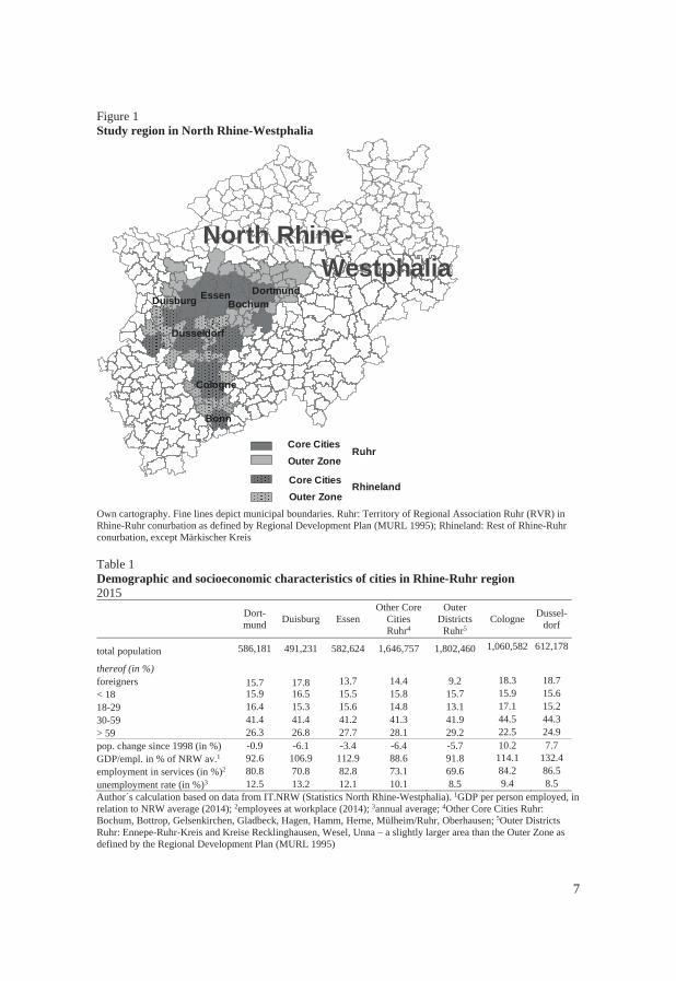
Due to a relatively advanced stage of ageing (Klemmer 2001) the Ruhr region in North

Rhine Westphalia serves as a likely case study. Comparison of the Ruhr (commonly

defined as the administrative area of the Ruhr Regional Association, RVR) with other

cities in the nearby Rhineland of North Rhine-Westphalia (Figure 1) highlights the

progress of ageing in the Ruhr. The large Rhineland cities Cologne and (particularly)

Düsseldorf rank high above the average of North Rhine-Westphalia with respect to

income (as measured in GDP per person employed). In these cities, there is also a

relatively high concentration of working-age residents and immigrants, in this case

represented by the share of foreign nationals (Table 1).

1 The identification strategy was developed by Berry et al. (1995) with respect to the US automobile industry. It was

applied to housing market analysis by Bayer et al. (2004).

7

Figure 1 Study region in North Rhine-Westphalia

Own cartography. Fine lines depict municipal boundaries. Ruhr: Territory of Regional Association Ruhr (RVR) in Rhine-Ruhr conurbation as defined by Regional Development Plan (MURL 1995); Rhineland: Rest of Rhine-Ruhr conurbation, except Märkischer Kreis

Table 1 Demographic and socioeconomic characteristics of cities in Rhine-Ruhr region 2015

Dort- mund Duisburg Essen

Other Core Cities Ruhr4

Outer Districts

Ruhr5 Cologne Dussel-

dorf

total population 586,181 491,231 582,624 1,646,757 1,802,460 1,060,582 612,178

thereof (in %) foreigners 15.7 17.8 13.7 14.4 9.2 18.3 18.7 < 18 15.9 16.5 15.5 15.8 15.7 15.9 15.6 18-29 16.4 15.3 15.6 14.8 13.1 17.1 15.2 30-59 41.4 41.4 41.2 41.3 41.9 44.5 44.3 > 59 26.3 26.8 27.7 28.1 29.2 22.5 24.9 pop. change since 1998 (in %) -0.9 -6.1 -3.4 -6.4 -5.7 10.2 7.7 GDP/empl. in % of NRW av.1 92.6 106.9 112.9 88.6 91.8 114.1 132.4 employment in services (in %)2 80.8 70.8 82.8 73.1 69.6 84.2 86.5 unemployment rate (in %)3 12.5 13.2 12.1 10.1 8.5 9.4 8.5 Author´s calculation based on data from IT.NRW (Statistics North Rhine-Westphalia). 1GDP per person employed, in relation to NRW average (2014); 2employees at workplace (2014); 3annual average; 4Other Core Cities Ruhr: Bochum, Bottrop, Gelsenkirchen, Gladbeck, Hagen, Hamm, Herne, Mülheim/Ruhr, Oberhausen; 5Outer Districts Ruhr: Ennepe-Ruhr-Kreis and Kreise Recklinghausen, Wesel, Unna – a slightly larger area than the Outer Zone as defined by the Regional Development Plan (MURL 1995)

Outer Zone

North Rhine-Westphalia

Core CitiesRuhr

Outer ZoneCore Cities Rhineland

Duisburg Essen

Dusseldorf

BochumDortmund

Cologne

Bonn

8

Cities from the Ruhr rank lower in labour productivity and in in the share of working-age

residents, but are characterised by a higher share of senior citizens aged above 60 (e.g. in

27.7% in Essen, but only 22.5% in Cologne). The share of seniors is even higher in

smaller core cities and particularly in the outer zone of the Ruhr (29.2%) than in the large

core cities.

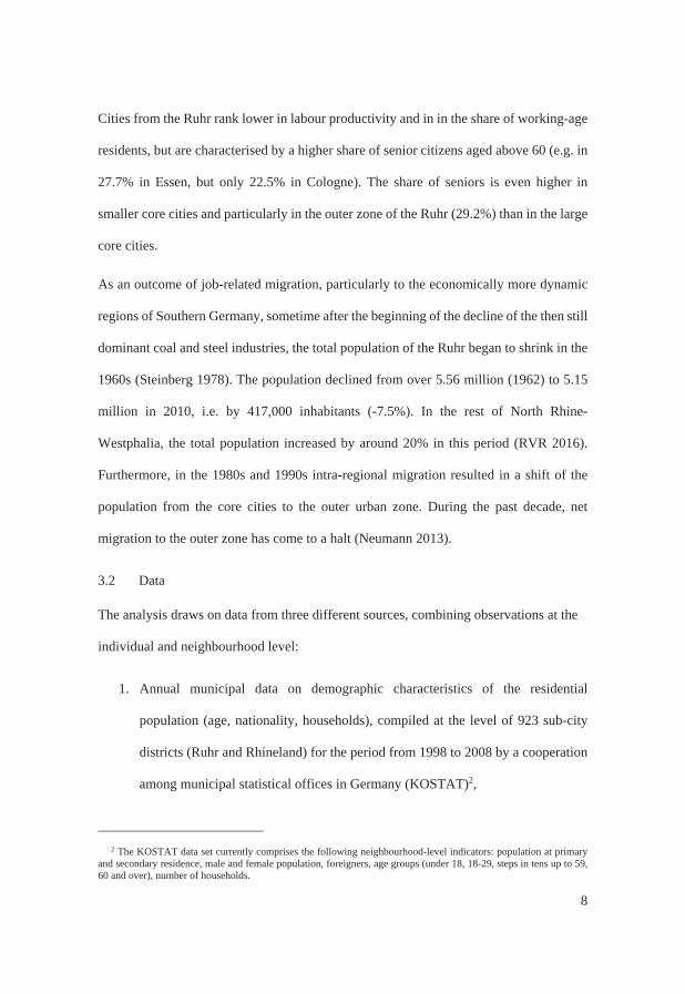
As an outcome of job-related migration, particularly to the economically more dynamic

regions of Southern Germany, sometime after the beginning of the decline of the then still

dominant coal and steel industries, the total population of the Ruhr began to shrink in the

1960s (Steinberg 1978). The population declined from over 5.56 million (1962) to 5.15

million in 2010, i.e. by 417,000 inhabitants (-7.5%). In the rest of North Rhine-

Westphalia, the total population increased by around 20% in this period (RVR 2016).

Furthermore, in the 1980s and 1990s intra-regional migration resulted in a shift of the

population from the core cities to the outer urban zone. During the past decade, net

migration to the outer zone has come to a halt (Neumann 2013).

3.2 Data

The analysis draws on data from three different sources, combining observations at the

individual and neighbourhood level:

1. Annual municipal data on demographic characteristics of the residential

population (age, nationality, households), compiled at the level of 923 sub-city

districts (Ruhr and Rhineland) for the period from 1998 to 2008 by a cooperation

among municipal statistical offices in Germany (KOSTAT)2,

2 The KOSTAT data set currently comprises the following neighbourhood-level indicators: population at primary

and secondary residence, male and female population, foreigners, age groups (under 18, 18-29, steps in tens up to 59, 60 and over), number of households.

9

2. Data on aggregate demographic neighbourhood and housing characteristics (in

2010) compiled by infas Institute of Applied Science3, and

3. Microdata from a representative survey4 among the (over 18-year-old) Ruhr

population in 2010 (3,237 observations).

Municipal sub-city districts (data source 1) represent historical “neighbourhoods“ or

housing estates, which are perceived as spatial entities5. On a voluntary basis, over 100

cities (almost all with more than 100,000 inhabitants) have agreed to cooperate in a

working group (KOSTAT) and to distribute a set of standardised sub-city data, which

comprises information about the total population, sex, nationality, age and households,

but conveys no direct reference to mobility (KOSIS Association Urban Audit (ed.) 2015).

In the Ruhr study region, on average around 10,000 inhabitants live in these statistical

districts. In addition, statistical data that covers a wider range of indicators (age,

households size, income, housing) and refers to smaller districts (with an average

population of around 1,300, representing a cross-section for 2010; data source 2) was

provided by infas, a market research firm. This district-level data was linked with

georeferenced microdata from a representative survey among the Ruhr population,

carried out in 2010 (data source 3).

While there is no direct information about housing costs available in the data sources used

in this analysis, a proxy for house prices is generated from information about housing

3 Infas calculates data on sub-entities of municipal districts (with an average population of around 1,300) based on

market research information compiled at the level of individual households and buildings (infas 2015). The dataset comprises demographic statistics for 2,318 districts.

4 The survey was carried out as part of a study on behalf of the RAG-Stiftung in 2010 (RWI 2011). 5Methodical challenges arise for regional analysis using aggregate data. These have been described as the modifiable

areal unit problem (MAUP) (Openshaw 1984). Municipal sub-city districts are assumed to represent intra-city differentials accurately, since they refer to those historical neighbourhoods, which are also referred to for purposes of municipal planning.

10

quality. A categorical variable characterising the type and quality of the housing stock in

the immediate vicinity of the residential location of survey participants was generated by

infas. Among a range of 53 categories, this typology separates between higher and lower

quality housing stock6. A high price is assumed where the housing stock in the immediate

vicinity of the residential location is assigned a high quality and in city centres, where

high prices can be expected (see above).

3.3 Approach

The following analysis proceeds in two steps, focussing on i. neighbourhood-level

demographic change, and ii. the household preferences relating to neighbourhood

attributes. The production of novel evidence at the population level in the first step is thus

complemented by testing how the migration and location decisions of households shape

the aggregate outcome (Billari 2015).

It can be assumed that neighbourhoods have certain unobserved advantages (or

disadvantages) making them attractive (or inattractive). In an analysis of demographic

change over a specific period that does not account for such unobservable characteristics,

it is likely for residuals to be correlated with any demographic outcome measure at the

level of spatial entities. A specification that eliminates these neighbourhood-specific

assets is the fixed effects approach, which utilises variation within individual districts

over time in the form of

6 The housing stock typology, which was registered for 2,891 survey participants, comprises the following

categories: farms, rural settlements, posh neighbourhood of stately mansions, older (pre 1970) high-quality low-density residential area, older lower quality low-density residential area, newer (post 1970) high quality low-density residential area, newer low quality low-density residential area, city centre, older high quality multi-family homes, newer high quality multi-family homes, older low-quality multi-family homes, older very low quality multi-family homes, special zones (nursing homes, barracks, hospitals). These are further subdivided according to the age of buildings and city size, resulting in 53 categories altogether.

11

(1) with i = 1,2,...N and t = 1, 2...11,

where Yit is the population of neighbourhood i at time t, Xit is a set of demographic

characteristics for each neighbourhood i, t comprises 11 observations for each year from

1998 to 2008, it is disturbance at time t7, is the average population of neighbourhood

i during all annual observations over the study period, the represent the corresponding

averages of demographic characteristics and the residuals, averaged over time. In the

following section 4, it will be investigated whether growth of the total population

combined with change in the share of selected age groups (< 18, 18-30) or the share of

immigrants among the neighbourhood residential population. They comprise newborn

children and, arguably, those demographic groups, which are most mobile in a regional

sense. Separate estimations according to equation (1) comprise the Ruhr and Rhineland

(Figure 1), in order to identify the specifics of the Ruhr as an ageing region. Spatial

autocorrelation in the residuals is accounted for by clustering standard errors at the level

of municipalities8.

In the analysis of household location preferences in section 5 it will be assumed that

households choose their specific residential location in terms of the indirect utility

function

(2)

in which

7Outliers were deleted from the dependent variable, i.e. the total neighbourhood population. The estimations

comprise observations between the 5th and the 95th percentiles of the dependent variable. In order to adjust for between-district differential in population size, the inverse of the total population is applied as a weight.

8 Due to exogenous factors affecting municipalities as a whole (e.g. public debt, house prices), residuals may be correlated among the neighbourhoods of a city. Assuming uncorrelated standard errors would imply underestimating variance and overestimating the statistical significance of coefficients.

12

(3) .

The identification strategy requires that the indirect utility of location choice, , as

characterised by equation (2), comprises household-specific parameters and mean

indirect utilities , which are common to all households9. In equation (3), the

represent the observable characteristics of housing choice , comprising attributes of the

house (e.g. one- or multi-family) and neighbourhood (e.g. residential, commercial).

represents average sociodemographic characteristics of the neighbourhood, which are

determined in a sorting equilibrium, in which households sort according to their budget

and preferences, and denotes the price of housing choice (which is a disutility).

comprises the proportion of unobserved preferences for housing and neighbourhood that

is correlated across households and represents idiosyncratic preferences.

Estimation of equations (2) and (3) follows a two-step procedure. Assuming that

households are sufficiently small not to interact strategically with respect to , the first

stage derives the preference parameters and choice-specific constants by estimation

of equation (2) in terms of a multinomial logit (MNL) model. In the literature on housing

choice, a variety of studies have found the MNL approach to be an appropriate empirical

framework (De Palma et al. 2005, Duncobe et al. 2001, Gabriel and Rosenthal 1999)10,

albeit fading out the feedback effects of household location decisions on neighbourhood

characteristics, if the estimation is restricted to the first stage , i.e. equation (2).

9In order to measure the mean indirect utility , all individual and household characteristics in the model are

constructed to have mean zero. The constant for the base category is set to zero. A test of the IIA properties according to the procedure suggested by Hausman and McFadden (1984) confirms applicability of the MNL estimation.

10A more comprehensive discussion of the methodical approach can be found in Neumann and Schmidt (2016).

13

The second stage estimates the mean taste parameters , using the alternative constants

from the first stage as dependent variable in the estimation of equation (3). Attributes of

housing and neighbourhood, , will be captured via the quality of local shopping

facilities, average socioeconomic characteristics will be determined by whether the

household resides in one of the four largest cities of the Ruhr (Bochum, Dortmund,

Duisburg, Essen) or in a smaller municipality.

Since house prices are likely to be correlated with unobserved neighbourhood

characteristics, in the second-stage estimation an instrument will be applied. Drawing on

the IV approach developed by Bayer et al. (2004), the instrument utilises the equilibrium

property of housing markets, in which the price of a house is determined not only by its

own characteristics and the demand for housing in its neighbourhood, but also by the

desirability of alternative houses and neighbourhoods in the region. In the analysis, the

housing quality at the non-chosen location alternatives, which affects equilibrium prices

but is uncorrelated with other neighbourhood characteristics determining the utility

gained from the location decision itself, therefore will serve as an instrument for housing

quality and price (see below).

For any combination of the household-specific parameters and mean indirect utilites

the model predicts the probability that household chooses location . Obviously,

definition of choice options may have a significant impact on the estimates of preference

parameters. Since consideration of the characteristics of all non-chosen housing locations

would render the estimation computationally intractable, it is common to focus on a

restricted range of alternatives. For example, Bayer et al. (2004) define the alternatives

from a 1-in-7 sample of non-chosen houses within the census district of the residential

location in the San Francisco Bay area. Tra (2010) applies a random sample of 15 non-

14

chosen alternatives from a set of around 5,000 housing types in the Los Angeles area in

his discrete choice equilibrium model of location preference.

In this analysis, the household´s choice set is restricted to three neighbourhood

alternatives defined by characteristic of the residential population and a fourth category

comprising all households not providing information about housing and neighbourhood

(Section 5). Separate categories are defined for core cities and outer zone, thus resulting

in eight neighbourhood choice options. In contrast to previous studies, which do not

usually control for the length of stay at the current residence, the analysis concentrates on

mobile households. Their preferences will be compared to those of households, which

had not relocated within a predefined time span before the interview in 2010.

4. Neighbourhood-level demographic change 1998-2008

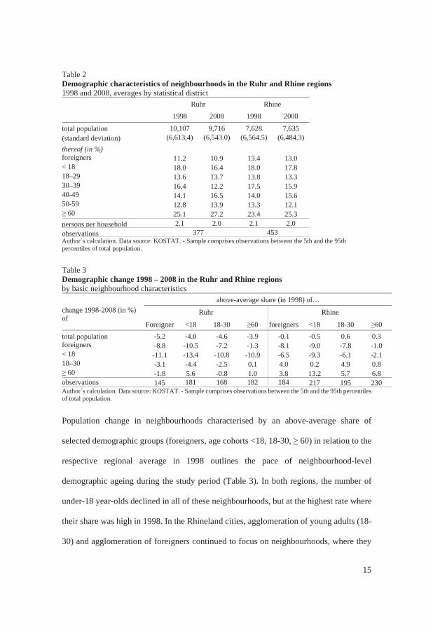
Over the survey period between 1998 and 2008, the total population of the Ruhr region

decreased from 5.25 million to 5.06 million (-3.6%), whereas the population of the

Rhineland (Figure 1) increased from just under 6 million to 6.02 million (+0.5%). On

average, the population of the Ruhr districts decreased from 10,107 (1998), to 9,716 in

2008, while the Rhineland district population increased from 7,628 to 7,635 (Table 2). In

both regions, in line with ageing of the “baby boomer” age cohorts born in the 1960s, the

share of the 30-40 year-olds decreased and that of the 40-50 age group increased between

1998 and 2008. In 2008, however, the share of 30-40 year-olds was still higher (15.9%)

in the Rhine than in the Ruhr (12.2%) region. Obviously, in the more prosperous Rhine

region younger working-age residents account for a larger share of the total residential

population.

15

Table 2 Demographic characteristics of neighbourhoods in the Ruhr and Rhine regions 1998 and 2008, averages by statistical district

Ruhr Rhine

1998 2008 1998 2008

total population 10,107 9,716 7,628 7,635 (standard deviation) (6,613,4) (6,543.0) (6,564.5) (6,484.3) thereof (in %) foreigners 11.2 10.9 13.4 13.0 < 18 18.0 16.4 18.0 17.8 18–29 13.6 13.7 13.8 13.3 30–39 16.4 12.2 17.5 15.9 40-49 14.1 16.5 14.0 15.6 50-59 12.8 13.9 13.3 12.1

60 25.1 27.2 23.4 25.3 persons per household 2.1 2.0 2.1 2.0 observations 377 453 Author´s calculation. Data source: KOSTAT. - Sample comprises observations between the 5th and the 95th percentiles of total population.

Table 3 Demographic change 1998 – 2008 in the Ruhr and Rhine regions by basic neighbourhood characteristics

above-average share (in 1998) of… change 1998-2008 (in %) of

Ruhr Rhine

Foreigner <18 18-30 60 foreigners <18 18-30 60 total population -5.2 -4.0 -4.6 -3.9 -0.1 -0.5 0.6 0.3 foreigners -8.8 -10.5 -7.2 -1.3 -8.1 -9.0 -7.8 -1.0 < 18 -11.1 -13.4 -10.8 -10.9 -6.5 -9.3 -6.1 -2.1 18–30 -3.1 -4.4 -2.5 0.1 4.0 0.2 4.9 0.8

60 -1.8 5.6 -0.8 1.0 3.8 13.2 5.7 6.8 observations 145 181 168 182 184 217 195 230 Author´s calculation. Data source: KOSTAT. - Sample comprises observations between the 5th and the 95th percentiles of total population.

Population change in neighbourhoods characterised by an above-average share of

selected demographic groups (foreigners, age cohorts <18, 18-30, 60) in relation to the

respective regional average in 1998 outlines the pace of neighbourhood-level

demographic ageing during the study period (Table 3). In both regions, the number of

under-18 year-olds declined in all of these neighbourhoods, but at the highest rate where

their share was high in 1998. In the Rhineland cities, agglomeration of young adults (18-

30) and agglomeration of foreigners continued to focus on neighbourhoods, where they

16

were overrepresented already in 1998. The total population increased in none of the

selected kinds of neighbourhood in the Ruhr. In the Rhineland, the population increased

in neighbourhoods with a high share of 18-30 year-olds (+0.6%) and in those with a high

share of seniors (+0.3%). The number of seniors ( 60) increased in all neighbourhood

types in the Rhineland, particularly (+13.2%) where the share of children (<18) was high

in 1998, but also where their share was high already. In the Ruhr, the number of seniors

also increased at the highest rate (+5.6%) in those neighbourhoods, where children were

overrepresented in 1998. Obviously, neighbourhoods with a high share of households

with children were among those where ageing, i.e. a decline in the number of children

and an increase in the number of seniors, proceeded most rapidly. During the period from

1998 to 2008, this rapid ageing of family-dominated neighbourhoods was even more

profound in the Rhineland than in the Ruhr.

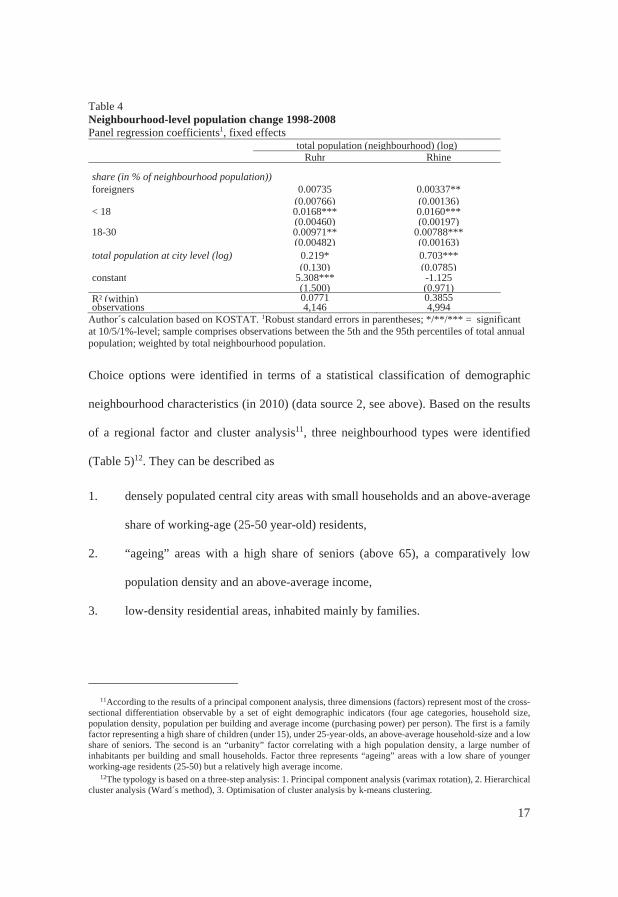
As expected, neighbourhood-level population growth between 1998 and 2008 coincided

with growth in the number of children, young adults, and (in the Rhineland) foreigners

(Table 4). The fixed effects regressions according to equation (1) therefore corroborate

fertility and the mobility of young adults (in contrast to the location choices of older age

groups) as components of neighbourhood population growth.

5. Regional migration and neighbourhood choice

5.1 Descriptive overview

For the purpose of analysing (intra-)regional migration and neighbourhood choice,

georeferenced micro-level information from a representative survey among the Ruhr

population, carried out in 2010, was combined with aggregate neighbourhood data,

provided by infas.

17

Table 4 Neighbourhood-level population change 1998-2008 Panel regression coefficients1, fixed effects

total population (neighbourhood) (log) Ruhr Rhine

share (in % of neighbourhood population)) foreigners 0.00735 0.00337** (0.00766) (0.00136) < 18 0.0168*** 0.0160*** (0.00460) (0.00197) 18-30 0.00971** 0.00788*** (0.00482) (0.00163) total population at city level (log) 0.219* 0.703*** (0.130) (0.0785) constant 5.308*** -1.125 (1.500) (0.971) R² (within) 0.0771 0.3855 observations 4,146 4,994

Author´s calculation based on KOSTAT. 1Robust standard errors in parentheses; */**/*** = significant at 10/5/1%-level; sample comprises observations between the 5th and the 95th percentiles of total annual population; weighted by total neighbourhood population.

Choice options were identified in terms of a statistical classification of demographic

neighbourhood characteristics (in 2010) (data source 2, see above). Based on the results

of a regional factor and cluster analysis11, three neighbourhood types were identified

(Table 5)12. They can be described as

1. densely populated central city areas with small households and an above-average

share of working-age (25-50 year-old) residents,

2. “ageing” areas with a high share of seniors (above 65), a comparatively low

population density and an above-average income,

3. low-density residential areas, inhabited mainly by families.

11According to the results of a principal component analysis, three dimensions (factors) represent most of the cross-

sectional differentiation observable by a set of eight demographic indicators (four age categories, household size, population density, population per building and average income (purchasing power) per person). The first is a family factor representing a high share of children (under 15), under 25-year-olds, an above-average household-size and a low share of seniors. The second is an “urbanity” factor correlating with a high population density, a large number of inhabitants per building and small households. Factor three represents “ageing” areas with a low share of younger working-age residents (25-50) but a relatively high average income.

12The typology is based on a three-step analysis: 1. Principal component analysis (varimax rotation), 2. Hierarchical cluster analysis (Ward´s method), 3. Optimisation of cluster analysis by k-means clustering.

18

Table 5 Demographic neighbourhood types of Ruhr region 2009

1 2 3 Total

“central” “ageing” “families”

total population 873,741 946,500 1,210,931 3,031,172 thereof (in %) under 15 12.5 11.8 15.7 13.6 15 – 25 10.1 9.3 13.8 11.3 25 – 50 35.9 34.9 33.8 34.8 50-65 19.6 20.8 17.8 19.3

65 21.9 23.2 18.8 21.1 population per km² 5,040 1,064 654 1,040 household size 1.9 2.1 2.1 2.0 persons per building 7.3 4.1 4.4 4.9 annual purchasing power (€/person) 17,919 19,744 17,983 18,514 Author´s calculation. Data source: infas regional data - Typology: 1 = city centre, 2 = ageing, 3 = families, n.a. = no neighbourhood information available. Cluster analysis (Ward´s method), optimised by k-means clustering using factor values of three factors derived from infas neighbourhood statistics

Since neighbourhood statistics was only provided for 2,318 out of 3,237 survey

participants, in the following a lack of neighbourhood information will be considered as

a separate category. “Migration” in the analysis refers to all individuals (the basic level

of observation is the individual), who had moved to the city, in which they lived in 2010,

during the previous 15 years13. This “mobile” group comprises 22% of the total survey

population, i.e. the vast majority had not moved across city boundaries for over 15 years.

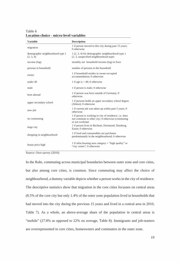
Analysis of individual-specific location preferences takes into account demographic

characteristics at the household (income, household size, homeownership) and individual

(age, migration background, job mobility, commuting) level (Table 6).

Taking up a new job, which is expected to be a main motive of migration, is considered

among the explanatory variables. A job is defined here as “new” if it was taken up within

five years before the survey.

13 Duration of residence in the current municipality was recorded in terms of six categories: 1. <6 months; 2. 6

months – 2 years; 3. 2-5 years; 4. 5-10 years; 5. 10-15 years; 6. >15 years. Categories 1-5 combined comprise 22% of all observations, category 6 accounts for 78%.

19

Table 6 Location choice - micro-level variables

Variable Description

migration 1 if person moved to this city during past 15 years; 0 otherwise

demographic neighbourhood type 1 (2, 3, 4)

1 (2, 3, 4) for demographic neighbourhood type 1 (2, 3, unspecified neighbourhood type)

income (log) monthly net household income (log) in Euro

persons in household number of persons in the household

owner 1 if household resides in owner-occupied accommodation; 0 otherwise

under 40 1 if age is < 40; 0 otherwise

male 1 if person is male; 0 otherwise

born abroad 1 if person was born outside of Germany; 0 otherwise

upper secondary school 1 if persons holds an upper secondary school degree (Abitur); 0 otherwise

new job 1 if current job was taken up within past 5 years; 0 otherwise

no commuting 1 if person is working in city of residence, i.e. does not commute to other city; 0 otherwise (commuting or not working)

large city 1 if person lives in Bochum, Dortmund, Duisburg, Essen; 0 otherwise

shopping in neighbourhood 1 if food and consumables are purchases predominantly in the neighbourhood; 0 otherwise

house price high 1 if infas housing area category = “high quality” or “city centre”; 0 otherwise

Source: Own survey (2010)

In the Ruhr, commuting across municipal boundaries between outer zone and core cities,

but also among core cities, is common. Since commuting may affect the choice of

neighbourhood, a dummy variable depicts whether a person works in the city of residence.

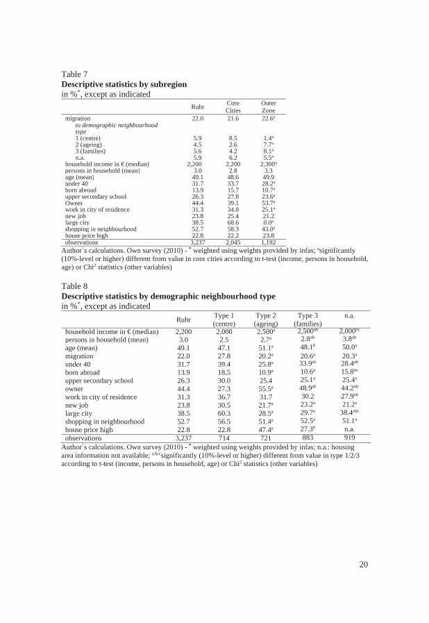
The descriptive statistics show that migration in the core cities focusses on central areas

(8.5% of the core city but only 1.4% of the outer zone population lived in households that

had moved into the city during the previous 15 years and lived in a central area in 2010,

Table 7). As a whole, an above-average share of the population in central areas is

“mobile” (27.8% as opposed to 22% on average, Table 8). Immigrants and job-starters

are overrepresented in core cities, homeowners and commuters in the outer zone.

20

Table 7 Descriptive statistics by subregion in %*, except as indicated

Ruhr Core Cities

Outer Zone

migration 22.0 21.6 22.6a to demographic neighbourhood type 1 (centre) 5.9 8.5 1.4a

2 (ageing) 4.5 2.6 7.7a

3 (families) 5.6 4.2 8.1a

n.a. 5.9 6.2 5.5a

household income in € (median) 2,200 2,200 2,300a

persons in household (mean) 3.0 2.8 3.3age (mean) 49.1 48.6 49.9under 40 31.7 33.7 28.2a

born abroad 13.9 15.7 10.7a

upper secondary school 26.3 27.8 23.6a

Owner 44.4 39.1 53.7a

work in city of residence 31.3 34.8 25.1a

new job 23.8 25.4 21.2large city 38.5 68.6 0.0a

shopping in neighbourhood 52.7 58.3 43.0a

house price high 22.8 22.2 23.8observations 3,237 2,045 1,192

Author´s calculations. Own survey (2010) - * weighted using weights provided by infas; asignificantly (10%-level or higher) different from value in core cities according to t-test (income, persons in household, age) or Chi2 statistics (other variables) Table 8 Descriptive statistics by demographic neighbourhood type in %*, except as indicated

Ruhr Type 1 (centre)

Type 2 (ageing)

Type 3 (families)

n.a.

household income in € (median) 2,200 2,000 2,500a 2,500ab 2,000bc

persons in household (mean) 3.0 2.5 2.7a 2.8ab 3.8ab

age (mean) 49.1 47.1 51.1a 48.1b 50.0a

migration 22.0 27.8 20.2a 20.6a 20.3a

under 40 31.7 39.4 25.8a 33.9ab 28.4ab

born abroad 13.9 18.5 10.9a 10.6a 15.8bc

upper secondary school 26.3 30.0 25.4 25.1a 25.4a

owner 44.4 27.3 55.5a 48.9ab 44.2ab

work in city of residence 31.3 36.7 31.7 30.2 27.9ab

new job 23.8 30.5 21.7a 23.2a 21.2a

large city 38.5 60.3 28.5a 29.7a 38.4abc

shopping in neighbourhood 52.7 56.5 51.4a 52.5a 51.1a

house price high 22.8 22.8 47.4a 27.3b n.a.observations 3,237 714 721 883 919

Author´s calculations. Own survey (2010) - * weighted using weights provided by infas; n.a.: housing area information not available; a/b/csignificantly (10%-level or higher) different from value in type 1/2/3 according to t-test (income, persons in household, age) or Chi2 statistics (other variables)

21

Table 9 Descriptive statistics, mobile and non-mobile individuals in %*, except as indicated

Ruhr migration = 1

migration = 0

household income in € (median) 2,200 2,000 2,300persons in household (mean) 3.0 2.8 3.0age (mean) 49.1 40.0 51.7a

under 40 31.7 52.6 25.8a

born abroad 13.9 26.5 10.3a

upper secondary school 26.3 35.1 23.8a

owner 44.4 31.7 48.0a

work in city of residence 31.3 29.3 31.8a

new job 23.8 39.8 19.4a

large city 38.5 39.9 38.1shopping in neighbourhood 52.7 48.2 54.0a

house price (too) high 22.8 25.2 22.1observations 3,237 744 2,493

Author´s calculations. Own survey (2010) - * weighted using weights provided by infas; 3,237 observations; asignificantly (10%-level or higher) different from value among mobile individuals (migration = 1) according to t-test (income, persons in household, age) or Chi2 statistics (other variables)

According to the survey from 2010, around 53% of the over 18 year-old Ruhr population

acquire food and consumables predominantly within their neighbourhood. Most other

goods are purchased outside of the neighbourhood, but within the city of residence. In the

following, households will be assumed to perceive neighbourhood amenities to be of high

quality if they shop locally. Among the more “mobile” group, working-age adults,

foreign-born persons and job-starters are overrepresented, whereas the share of

homeowners, the average household income and the average age of household members

are lower than among the “non-mobile” population (Table 9)14.

5.2 Household-specific preferences (first stage of the estimation)

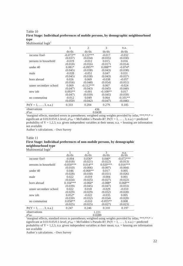
Among households moving to central areas (type 1), there was an above-average share of

young adults and job-starters (who are unlikely to move to family areas, type 3) (Table

10).

14 Since homeownership correlates with income, housing cost and residential location, it will not be controlled for

in the analysis. In contrast to the U.S., where the tenure status is one of the key characteristics of housing quality, segregation between housing for rent and for sale is less distinguished.

22

Table 10 First Stage: Individual preferences of mobile persons, by demographic neighbourhood typeMultinomial logit1

1 2 3 n.a. dy/dx dy/dx dy/dx dy/dx

income (log) -0.073** 0.122*** -0.017 -0.032 (0.037) (0.034) (0.035) (0.030)persons in household -0.019 -0.012 0.015 0.016 (0.018) (0.016) (0.017) (0.014)under 40 0.081* -0.095** 0.088** -0.074* (0.045) (0.038) (0.043) (0.038)male -0.028 -0.051 0.047 0.031 (0.045) (0.038) (0.043) (0.037)born abroad 0.026 0.069 -0.038 -0.057 (0.056) (0.048) (0.054) (0.051)upper secondary school 0.069 -0.112*** 0.067 -0.024 (0.047) (0.043) (0.045) (0.040)new job 0.093** -0.001 -0.108** 0.017 (0.047) (0.039) (0.045) (0.039)no commuting -0.012 0.049 0.064 -0.101** (0.050) (0.042) (0.047) (0.046)

Pr(Y = 1, … , 3, n.a.) 0.333 0.204 0.279 0.185 observations 436p²MF 0.04381marginal effects, standard errors in parentheses; weighted using weights provided by infas, ***/**/* = significant at 0.01/0.05/0.1-level, p²MF = McFadden´s Pseudo-R²; Pr(Y = 1, … , 3, n.a.) = predicted probability of Y = 1,2,3, n.a. given independent variables at their mean; n.a. = housing are information not available Author´s calculations. - Own Survey Table 11 First Stage: Individual preferences of non-mobile persons, by demographic neighbourhood type Multinomial logit1

1 2 3 n.a. dy/dx dy/dx dy/dx dy/dx

income (log) -0.004 0.036* 0.040* -0.072*** (0.018) (0.021) (0.022) (0.013)persons in household -0.050*** 0.014** 0.020*** 0.016*** (0.010) (0.006) (0.007) (0.004)under 40 0.046 -0.068** 0.017 0.005 (0.028) (0.030) (0.031) (0.026)male 0.022 -0.019 -0.004 0.001 (0.024) (0.025) (0.027) (0.022)born abroad 0.104*** -0.084* -0.088* 0.068** (0.039) (0.045) (0.047) (0.033)upper secondary school 0.022 0.018 -0.029 -0.010 (0.029) (0.029) (0.032) (0.028)new job 0.052* -0.022 -0.035 0.005 (0.030) (0.032) (0.034) (0.028)no commuting 0.058** -0.010 -0.055** 0.008 (0.025) (0.025) (0.027) (0.023)

Pr(Y = 1, … , 3, n.a.) 0.247 0.246 0.310 0.197 observations 1,221p²MF 0.02891marginal effects, standard errors in parentheses; weighted using weights provided by infas; ***/**/* = significant at 0.01/0.05/0.1-level, p²MF = McFadden´s Pseudo-R²; Pr(Y = 1, … , 3, n.a.) = predicted probability of Y = 1,2,3, n.a. given independent variables at their mean; n.a. = housing are information not available Author´s calculations. - Own Survey

23

Households moving to ageing areas (type 2) earned an above-average income and are

more likely to own their dwelling. Working-age adults (18-40) are underrepresented

among households choosing to locate in ageing areas. For households that were “mobile”

in the 15 years before the survey, the average probability of choosing central areas (type

1) as residential location (33%) was higher than the probability of choosing types 2 or 3.

Households that had not crossed city boundaries, on the other hand, were most likely to

reside in “family” areas (type 3).

In comparison, “mobile” individuals sort across neighbourhood types more distinctly than

others by age and education, since they are relatively unlikely to settle in “ageing” areas.

“Non-mobile” households, on the other hand, are sorted more distinctly by household

size, provenance and commuting. Among the “non-mobile” group larger households

prefer “ageing” or “family” type areas, immigrants are unlikely to settle anywhere but in

central areas and commuting is unlikely for people living in central quarters but likely for

those in family neighbourhoods (Table 11).

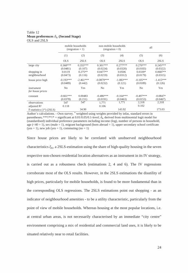
5.3 Mean preferences (second stage of the estimation)

Given the individual-specific preferences of all households, persons living in one of the

largest cities (Bochum, Dortmund, Duisburg or Essen) are likely to have chosen a highly

popular choice option, i.e. a central area, as residential location. While the desirability of

central locations has increased, so has residence in a large city, as comparison between

“mobile” and “non-mobile” households reveals (Table 12). It is unlikely, however, for

households at such popular locations to dwell in high-cost housing15.

15 Apparently, only 8.7% of persons living in mobile households in type 1 (central area) actually reside in housing

classified as “city centre“ by the infas housing category. It is plausible therefore that residence in the most popular neighbourhood type, i.e. type 1 (central areas) rarely combines with the “high price“ housing category, of which the infas “city centre“ housing category is part. Most people in type 1 apparently live in housing that is near to centres, but not necessarly located in a mixed residential/commercial housing environment.

24

Table 12 Mean preferences (Second Stage) OLS and 2SLS

mobile households (migration = 1)

non-mobile households (migration = 0) all

(1) (2) (3) (4) (5) (6)

OLS 2SLS OLS 2SLS OLS 2SLS large city 0.368*** 0.355*** 0.301*** 0.277*** 0.270*** 0.245*** (0.0481) (0.107) (0.0224) (0.0320) (0.0183) (0.0322) shopping in 0.0119 0.275** 0.0477** 0.0506 0.0339* 0.0687** neighbourhood (0.0473) (0.116) (0.0219) (0.0312) (0.0179) (0.0315)

house price high -0.193*** -2.461*** -0.0879*** -1.083*** -0.105*** -1.415*** (0.0489) (0.442) (0.0232) (0.121) (0.0189) (0.126)

instrument No Yes No Yes No Yes for house prices

constant -0.661*** 0.00483 -0.486*** -0.164*** -0.497*** -0.0847* (0.0378) (0.151) (0.0191) (0.0463) (0.0153) (0.0467) observations 547 547 1,771 1,771 2,318 2,318adjusted R² 0.118 0.106 0.102 F-statistics (1st) (2SLS) 34.90 143.92 173.03

Author´s calculations. - Own survey. * weighted using weights provided by infas, standard errors in parentheses; ***/**/* = significant at 0.01/0.05/0.1-level; derived from multinomial logit model for (standardised) individual preference parameters including income (log), number of persons in household, age (<40 = 1), sex (male = 1), migrant background (born abroad = 1), upper secondary school certificate (yes = 1), new job (yes = 1), commuting (no = 1)

Since house prices are likely to be correlated with unobserved neighbourhood

characteristics , a 2SLS-estimation using the share of high-quality housing in the seven

respective non-chosen residential location alternatives as an instrument in its IV strategy,

is carried out as a robustness check (estimations 2, 4 and 6). The IV regressions

corroborate most of the OLS results. However, in the 2SLS estimations the disutility of

high prices, particularly for mobile households, is found to be more fundamental than in

the corresponding OLS regressions. The 2SLS estimations point out shopping - as an

indicator of neighbourhood amenities - to be a utility characteristic, particularly from the

point of view of mobile households. Whereas housing at the most popular locations, i.e.

at central urban areas, is not necessarily characterised by an immediate “city centre”

environment comprising a mix of residential and commercial land uses, it is likely to be

situated relatively near to retail facilities.

25

5. Conclusions

In the Ruhr region over the past decades demographic change coincided with a strong

preference of mobile households for central locations. After several decades of

suburbanisation, in the 1990s net migration to suburban municipalities came to a halt.

Within urban areas, mobility now concentrates more on selected neighbourhoods in close

vicinity to the city centres. In other neighbourhoods, due to low fertility and a

comparatively low influx of mobile households, the average age has begun to increase.

Since the location choices of younger adults focused more on central areas, “ageing by

feet” implies changes in the degree to which certain goods or services are perceived to be

desirable and “scarce” within neighbourhoods. This may affect, specifically, ageing

neighbourhoods characterised by low-density housing, where local communities so far

have been accustomed with the provision of amenities for growing populations. An

increasing agglomeration of younger, working-age residents in central city areas might

attract even more young people and, in turn, accelerate ageing of the less popular

neighbourhoods. Adaptation of local markets for housing, services and retail to an ageing

population will provide an additional incentive for younger generations to leave or to

avoid moving to ageing neighbourhoods.

In comparison with the more prosperous nearby Rhinefront cities (Bonn, Cologne,

Düsseldorf), however, so far a comparatively lower agglomeration of working-age

residents has emerged in the central areas of large cities of the Ruhr region and “ageing

by feet” of low-density residential areas proceeds at a slower pace, even though ageing

of the region as a whole is more advanced. Possibly, this somewhat more balanced

progress of ageing across neighbourhoods in the Ruhr can be explained in part by its

settlement geography. It is a specific characteristic of the Ruhr to be less densely

26

populated than other urban agglomerations in Germany. Less overall density makes it

easier for different types of housing environment (e.g. low- and high density, purely

residential and mixed residential/commercial) to co-exist in close vicinity, even in core

cities. The Ruhr therefore may be better equipped than other regions to avoid

neighbourhood-level demographic segregation while adapting to ageing.

Part of the greater mix of generations and household types in the Ruhr, on the other hand,

is also due to a comparatively lower influx of working-age residents than to the more

prosperous Rhineland cities. Economic change and revitalisation of the Ruhr, which is

still in progress, therefore could combine with greater demographic segregation. All in

all, greater neighbourhood-level demographic variety, which is, in part, an outcome of

lower regional prosperity, may become an economic advantage for the Ruhr, if the word

gets around and mobile households appreciate this diversity as an asset.

References

Alonso, W. (1964), Location and land use: Toward a theory of land rent. Cam-bridge, Mass.: HUP.

Bayer, P., R. McMillan and K. Rueben (2004), An equilibrium model of sorting in an urban housing market. NBER Working Paper 10865. Cambridge, MA: NBER.

Berry, S., J. Levinsohn and A. Pakes (1995), Automobile prices in market equilibrium. Econometrica 64(4): 841-890.

Billari, F.C. (2015), Integrating macro- and micro-level approaches in the explanation of population change. Population Studies 69 (S1): S1-S12.

Boehm, T.P., Herzog Jr., H. W. and Schlottmann, A. M. (1991), Intra-urban mobility, migration and tenure choice. Review of Economics and Statistics 73(1): 59–68.

Coulson, M.R.C. (1968), The distribution of population age structures in Kansas City. Annals, Association of American Geographers 58(1): 155-176.

Coulter, R. and J. Scott (2015), What motivates residential mobility? Re-examining self-reported reasons for desiring and making residential moves. Population, Space and Place 21(4): 354-371.

De Palma, A., K. Motademi, N. Picard and P. Waddell (2005), A model of residential location choice with endogenous housing prices and traffic for the Paris region. EuropeanTransport 31/XI: 67-82.

27

Duncobe, W., M. Robbins and D. Wolf (2001), Retire to Where? A Discrete Choice Model of Residential Location. International Journal of Population Geography 7(4): 281-293.

Epple, D and H. Sieg (1999), Estimating equilibrium models of local jurisdictions. Journal of Political Economy 107(141): 645-681.

Gabriel, S.A. and S.S. Rosenthal (1999), Household location and race: Estimates of a multinomial logit model. Review of Economics and Statistics 71(2): 240-249.

Hausman, J.A. and D.L. McFadden (1984) Specification tests for the multinomial logit model. Econometrica 52(5), 1219-1240.

Hedman, L. (2013), Moving near family? The influence of extended family on neighbourhood choice in an intra-urban context. Population, Space and Place 19(1): 32-45.

Heinritz, G., and E. Lichtenberger (1991), Wien und München – ein stadtgeographischer Vergleich. Berichte zur deutschen Landeskunde 58(1): 55-95.

infas Institute of Applied Science (2015), infas 360. Orientierung für Ihr Kunden- und Adressmanagement. Bonn. Internet: www.infas360.de; accessed 25 June 2015.

Jackman, R. and S. Savouri (1992), Regional migration in Britain. An analysis of gross flows using NHS central register data. Economic Journal 102(415): 1433-1450.

Klemmer, P. (2001), Steht das Ruhrgebiet vor einer demographischen Herausforderung? Schriften und Materialien zur Regionalforschung 7. Essen: RWI.

Kley, S. (2010), Explaining the stages of migration within a life-course framework. European Sociological Review 27(4): 469-486.

KOSIS Association Urban Audit (ed.) (2015), The German Urban Audit. Data – indicators – information. Mannheim: Municipal Statistics Office.

Knox, P. and S. Pinch (2010), Urban social geography. An introduction. 6th ed. Harlow: Pearson.

Kuminoff, N.V, V.K. Smith and C. Timmins (2013), The new economics of equilibrium sorting and policy evaluation using housing markets. Journal of Economic Literature 51(4): 1007-1062.

MURL Ministerium für Umwelt, Raumordnung und Landwirtschaft des Landes Nordrhein-Westfalen (1995), LEP NRW. Landesentwicklungsplan Nordrhein-Westfalen. Düsseldorf: MURL.

Neumann, U. (2013), Are My Neighbours Ageing Yet? Local Dimensions of Demographic Change in German Cities. Journal of Population Ageing 6(3): 189-209.

Neumann, U. and C.M. Schmidt (2016), Regional migration and neighbourhood sorting. A discrete choice model of housing preferences in Germany. Ruhr Economic Papers (forthcoming).

O´Loughlin, J. and G. Glebe (1984), Intraurban migration in West German cities. Geographical Review 74(1): 1-23.

RVR Regionalverband Ruhr (2016), Zahlenspiegel metropoleruhr. Internet: www.metropoleruhr.de; accessed 11 April 2016.

28

RWI (2011), Den Wandel gestalten? Anreize für mehr Kooperationen im Ruhrgebiet. Projekt im Auftrag der RAG-Stiftung. RWI Projektberichte. Essen.

Steinberg, H. (1978). Bevölkerungsentwicklung des Ruhrgebiets im 19. und 20. Jahrhundert. Düsseldorfer Geographische Schriften 11. Düsseldorf: Geogr. Inst.

Tiebout, C.M. (1956), A pure theory of local expenditures. Journal of Political Economy 64(5): 416–424.

Data sources

infas regional data: Neighbourhood statistics for Ruhr survey area, 2009, provided by infas Institute of Applied Science, Bonn.

IT.NRW: Landesdatenbank NRW. Internet: www.landesdatenbank.nrw.de; accessed 8 November 2016.

KOSTAT: Municipal statistical data for sub-city districts, provided by KOSIS Association KOSTAT, Bremen. Annual time series, 1998-2008.

Own survey: Representative Population Survey carried out as part of a study by RWI on behalf of the RAG-Stiftung in 2010. Design weights provided by infas Institute of Applied Science, Bonn.