Age Classification using Facial Feature Extraction

Age Classification using Facial Feature Extraction

Fatemeh Mirzaei

Submitted to the Institute of Graduate Studies and Research

in partial fulfillment of the requirements for the Degree of

Master of Science

in Computer Engineering

Eastern Mediterranean University January 2011

Gazimağusa, North Cyprus

Approval of the Institute of Graduate Studies and Research

Prof. Dr. Elvan Yılmaz Director (a) I certify that this thesis satisfies the requirements as a thesis for the degree of Master of Science in Computer Engineering.

Assoc. Prof. Dr. Muhammed Salamah

Chair, Department of Computer Engineering We certify that we have read this thesis and that in our opinion it is fully adequate in scope and quality as a thesis for the degree of Master of Science in Computer Engineering.

Asst. Prof. Dr. Önsen Toygar

Supervisor

Examining Committee

1. Assoc. Prof. Dr. Hasan Demirel 2. Asst. Prof. Dr. Önsen Toygar

3. Asst. Prof. Dr. Ahmet Ünveren

iii

ABSTRACT

This thesis presents age classification on facial images using Local Binary Patterns

(LBP) and modular Principal Component Analysis (mPCA) as subpattern-based

approaches and holistic Principal Component Analysis (PCA) and holistic subspace

Linear Discriminant Analysis (ssLDA) methods. Classification of age intervals are

conducted separately on female and male facial images since the aging process for

female and male is different for human beings in real life. The age classification

performance of the holistic approaches is compared with the performance of

subpattern-based LBP and mPCA approaches in order to demonstrate the

performance differences between these two types of approaches. Our work has been

tested on two aging databases namely FGNET and MORPH. The experiments are

performed on these aging databases to demonstrate the age classification

performance on female and male facial images of human beings using subpattern-

based LBP method with several parameter settings. The results are then compared

with the results of age classification using mPCA method, holistic PCA and subspace

LDA methods.

Keywords – Age Classification, Local Binary Patterns, Modular Principal

Component Analysis, Principal Component Analysis, Subspace Linear Discriminant

Analysis.

iv

ÖZ

Bu tezde alt-örüntüye dayalı Yerel İkili Örüntü (LBP) ve modüler Ana Bileşenler

Analizi (mPCA) yaklaşımlarının yanısıra bütünsel Ana Bileşenler Analizi (PCA) ve

altuzay Doğrusal Ayırtaç Analizi (ssLDA) yöntemleri kullanılarak yüz resimlerinin

yaş sınıflandırması sunulmuştur. Gerçek hayatta kadın ve erkeklerin yaşlanma süreci

farklı olduğundan dolayı, yaş aralıklarının belirlenmesi kadın ve erkek resimleri

üzerinde ayrı olarak incelenmiştir. Alt-örüntüye dayalı LBP ve mPCA

yaklaşımlarının yaş sınıflandırma performansı, bütünsel yaklaşımlarla karşılaştırılmış

ve bu iki çeşit yaklaşımın performans farklılıkları sunulmuştur. Bu çalışmadaki

deneyler yaygın olarak kullanılan FGNET ve MORPH isimli yaşlanma veritabanları

üzerinde yapılmıştır. Kadın ve erkek resimleri kullanılarak yapılan yaş

sınıflandırmasının performansını göstermek için alt-örüntüye dayalı LBP yöntemi

değişik parametre değerleri ile yaşlanma veritabanları kullanılarak çalıştırılmıştır. Bu

deneylerin sonuçları daha sonra mPCA, bütünsel PCA ve altuzay LDA yöntemleri

kullanılarak yapılan yaş sınıflandırması deney sonuçlarıyla karşılaştırılmıştır.

Anahtar Kelimeler: Yaş Sınıflandırması, Yerel İkili Örüntü, modüler

Ana Bileşenler Analizi, Ana Bileşenler Analizi, Altuzay Doğrusal Ayırtaç Analizi.

v

DEDICATION

This is a dedication to the love of my life, My Husband, I would like to Thank You

for 2 and half wonderful years, through all the ups and downs. You’re Still The One.

I also dedicate this thesis to my BELOVED PARENTS, who are a part of my heart,

and I will be grateful all the days of my life for having had the honor to be your

daughter.

vi

ACKNOWLEDGMENTS

The sincere thanks go to my advisor Asst. Prof. Dr. Önsen Toygar whose patience

and encouragement guided me during the research. This dissertation would never be

possible without her helps. To me, she is not only the perfect mentor but also a true

friend. I also thank Assoc. Prof. Dr. Hasan Demirel and Asst. Prof. Dr. Ahmet

Ünveren for serving on my thesis committee.

My warmest thank to my dear husband, Amin. Whenever I encounter the difficulties

and disappointment, he always consoled me with the cordial warmth. He gave me

confident to go on and never hesitates to patiently assist me through the master study.

I am blessed to have him by my side and in my life.

I would like to express my heart-felt gratitude to my dear parents for their constant

source of love, patients and encouragements through my life.

vii

TABLE OF CONTENTS

ABSTRACT ............................................................................................................... iii

ÖZ ................................................................................................................................ iv

DEDICATION ............................................................................................................. v

ACKNOWLEDGMENTS ........................................................................................... vi

TABLE OF CONTENTS ........................................................................................... vii

LIST OF TABLES ....................................................................................................... x

LIST OF FIGURES .................................................................................................. xiii

1 INTRODUCTION ..................................................................................................... 1

1.1 Motivation .......................................................................................................... 1

1.1.1 Age-Based Access Control .......................................................................... 1

1.1.2 Age Specific Human Computer Interaction (ASHCI) ................................. 2

1.1.3 Age Invariant Person Identification ............................................................. 2

1.1.4 Data Mining and Organization .................................................................... 2

1.2 Related Works .................................................................................................... 2

1.3 Overview ............................................................................................................ 5

1.3.1 Age Classification from Facial Images ....................................................... 6

1.4 The Work Done In This Study ........................................................................... 7

2 PREPROCCESSING ............................................................................................... 11

2.1 Cropping Images .............................................................................................. 12

2.2 Resizing and Interpolation of Images ............................................................... 13

2.3 Histogram Equalization .................................................................................... 13

viii

2.4 Mean-Variance Normalization ......................................................................... 16

3 FEATURE EXTRACTION ..................................................................................... 18

3.1 Subpattern-based Approaches .......................................................................... 20

3.1.1 Local Binary Patterns (LBP) ..................................................................... 20

3.1.1.1 Local Binary Patterns (LBP) Algorithm ................................................. 21

3.1.2 Modular Principal Component Analysis (mPCA) ..................................... 25

3.1.2.1 Modular Principal Component Analysis (mPCA) Algorithm ................ 25

3.2 Holistic Approaches ......................................................................................... 26

3.2.1 Principal Component Analysis (PCA) ....................................................... 28

3.2.1.1 Principal Component Analysis (PCA) Algorithm .................................. 29

3.2.2 Subspace Linear Discriminant Analysis (ssLDA) ..................................... 29

3.2.2.1 Subspace Linear Discriminent Analysis (ssLDA) Algorithm ................ 31

4 GEOMETRY ANALYSIS ...................................................................................... 33

4.1 Geometric Variation ......................................................................................... 33

4.2 Ratio Analysis .................................................................................................. 34

4.2.1 Algorithm Using Ratio Analysis ............................................................... 35

5 EXPERIMENTS AND RESULTS .......................................................................... 38

5.1 Description of Databases .................................................................................. 39

5.1.1 FG-NET Aging Database .......................................................................... 39

5.2 First Step Age Classification Experiments on facial images ............................ 41

5.2.1 Experiments Using Subpattern-based Approaches ................................... 42

5.2.1.1 Experiments Using LBP ......................................................................... 42

5.2.1.2 Experiments Using mPCA ..................................................................... 49

5.2.2 Experiments Using Holistic Approaches ................................................... 51

5.2.2.1 Experiments Using PCA ......................................................................... 51

ix

5.2.2.2 Experiments Using ssLDA ..................................................................... 52

5.3 Second Step Age Classification Experiments on facial images ....................... 53

5.3.1 Experiments Using LBP ............................................................................ 54

5.3.2 Experiments Using mPCA ........................................................................ 56

5.3.3 Experiments Using PCA ............................................................................ 58

5.3.4 Experiments Using ssLDA ........................................................................ 59

5.4 Ratio Analysis .................................................................................................. 60

5.4.1 Age classification Experiments using two ratios ....................................... 60

6 CONCLUSION ....................................................................................................... 66

REFERENCES ........................................................................................................... 68

x

LIST OF TABLES

Table 5.1:Number of training and test images in 3 subsets ........................................ 41

Table 5.2: Female Age Classification Rates (%) with LBP on FGNET dataset ....... 43

Table 5.3: Female Age Classification Rates (%) with LBP on MORPH dataset ....... 44

Table 5.4: Female Age Classification Rates (%) with LBP on FGNET+MORPH

dataset ...................................................................................................... 45

Table 5.5: Male Age Classification Rates (%) with LBP on FGNET dataset ............ 46

Table 5.6: Male Age Classification Rates (%) with LBP on MORPH dataset .......... 47

Table 5.7: Male Age Classification Rates (%) with LBP on FGNET+MORPH dataset

................................................................................................................. 48

Table 5.8: Female and Male Age Classification Rates (%) with mPCA on FGNET

dataset ...................................................................................................... 49

Table 5.9: Female and Male Age Classification Rates (%) with mPCA on MORPH

dataset ...................................................................................................... 50

Table 5.10: Female and Male Age Classification Rates (%) with mPCA on

FGNET+MORPH dataset ........................................................................ 50

Table 5.11: Female and Male Age Classification Rates (%) with PCA on 3 datasets

................................................................................................................. 51

Table 5.12: Female and Male Age Classification Rates (%) with ssLDA on 3 datasets

................................................................................................................. 52

Table 5.13: Female Age Classification with LBP, mPCA, PCA, ssLDA .................. 53

xi

Table 5.14: Male Age Classification with LBP, mPCA, PCA, ssLDA ...................... 53

Table 5.15: Female, Male and Female+Male Second Step Age Classification Rates

(%) with LBP on FGNET dataset ............................................................ 54


(%) with LBP on MORPH dataset .......................................................... 55


(%) with LBP on FGNET+MORPH dataset ........................................... 55

Table 5.18: Female and Male Second Step Age Classification Rates (%) with mPCA

on FGNET dataset ................................................................................... 56


on MORPH dataset .................................................................................. 57


on FGNET+MORPH dataset ................................................................... 57


(%) with PCA on FGNET dataset ........................................................... 58


(%) with PCA on MORPH dataset .......................................................... 58


(%) with PCA on FGNET+MORPH dataset ........................................... 59

Table 5.24: Female and Male Second Step Age Classification Rates (%) with ssLDA

on FGNET MORPH and FGNET+MORPH dataset ............................... 59

Table 5.25: Baby Recognition Rates (%) with two Ratio analysis on FGNET dataset

................................................................................................................. 61

xii

Table 5.26: Ratio1 and Ratio2 values of some FGNET images ................................. 62

Table 5.27: Ratio values of MORPH images ............................................................. 64

xiii

LIST OF FIGURES

Figure 1.1: An illustration of the effects of applying different transformation

functions on ‘profile faces’ [9]. ................................................................. 6

Figure 1.2: Difference in Illumination (a) Brighter image (b) Darker image .............. 8

Figure 1.3: Difference in Pose (a) Frontal image (b) Profile image with some angle. 8

Figure 1.4: Difference in Facial Expression (a) Angry Face (b) Happy Face. ............. 8

Figure 1.5: Difference in Facial Texture (a) Image without wrinkles (b) Image with

wrinkles. .................................................................................................... 9

Figure 1.6: Difference in Facial Texture (a) Normal Face (b) Makeup Face ............... 9

Figure 1.7: Difference in Facial Hair (a) Face without mustache and beard (b) Face

with mustache and beard. .......................................................................... 9

Figure 1.8: Presence of Partial Occlusions (a) Face without glasses (b) Face with

glasses. ....................................................................................................... 9

Figure 2.1: Preprocessing steps on images ................................................................. 11

Figure 2.2: Original (A) and cropped (B) images from FGNET database ................. 12

Figure 2.3: Original and rotated image ....................................................................... 13

Figure 2.4: Histograms of dark image before and after histogram equalization ........ 14

Figure 2.5: Histograms of bright image before and after histogram equalization ...... 15

Figure 2.6: Sample images before (A & B) and after (C & D) histogram equalization

................................................................................................................. 16

xiv

Figure 3.1: Examples of facial images with different number of regions (25, 36, 49,

64, 81 partitions) ...................................................................................... 20

Figure 3.2: Example of circular neighborhoods. ........................................................ 21

Figure 3.3: An example of LBP computation ............................................................ 23

Figures 3.4: The basic LBP operator .......................................................................... 23

Figure 3.5: Histogram of image after concatenating all histograms .......................... 24

Figure 3.6: a) Original Image, b) LBP Image ............................................................ 24

Figure 3.7: Samples of cropped facial images ............................................................ 27

Figure 3.8: Facial images of three different age intervals selected from FG-NET

aging database .......................................................................................... 30

Figure 4.1: Variation of distance between primary features ...................................... 34

Figure 4.2: Six different ratios [2]. ............................................................................. 35

Figure 4.3: FGNET facial image with located and labeled feature points ................. 36

Figure 5.1: Training phase steps ................................................................................. 40

Figure 5.2: Test phase steps ........................................................................................ 40

Figure 5.3: Classification step .................................................................................... 40

1

Chapter 1

INTRODUCTION

Face images convey a significant amount of information including information about

the identity, emotional state, ethnic origin, gender, age, and head orientation of a

person shown in a face image [1]. In this study the age interval of facial images is

extracted for age classification purpose. Age classification has been studied in the

literature either as classification of age intervals to estimate an age group or as age

estimation to estimate an exact age. Some of the applications of age classification are

listed below.

1.1 Motivation

There are lots of applications that can benefit from automated systems. Age

determination can be used in a variety of applications ranging from access control,

human machine interaction, person identification, data mining and organization.

Examples can demonstrate some uses of the aging software for each category

mentioned above.

1.1.1 Age-Based Access Control

Age-based restrictions apply to physical or virtual access in some real life

applications. For example age-related entrance restrictions may apply to different

premises, web pages or even for preventing the purchase of certain goods (e.g.

alcoholic drinks or cigarettes) by under-aged individuals [3]. Secure Internet access

control is another example in order to ensure that under-aged persons can not access

to Internet pages with unsuitable material.

2

1.1.2 Age Specific Human Computer Interaction (ASHCI)

If computers could determine the age of the user, both the computing environment

and the type of interaction could be adjusted according to the age of the user [1].

Automatically adjusting the user interface of the computer or machine users to suit

the needs of users age group is one of the applications in ASHCI [31]. For example,

text and icons of the interface can be changed according to the users age, if he or she

is old the text with large font will be more suitable. On the other hand icons could be

more activated for young users. So persons with different age groups have different

requirements and needs related to the way they interact with computers or other

machines.

1.1.3 Age Invariant Person Identification

Automatic age estimation systems could form the basis of designing automatic age

progression systems. (i.e., systems with the ability to predict the future facial

appearance of subjects). One of the most popular applications of age progression

systems is “Missing Children” and it creates an image to investigate what a missing

child would look like today [1].

1.1.4 Data Mining and Organization

Age-based retrieval and classification would enable the users to automatically sort

and retrieve the images from e-photo albums and the Internet by specifying a

required age-range [31].

1.2 Related Works

Age classification has been studied in the literature either as classification of age

intervals to estimate an age group or as age estimation to estimate an exact age. Age

classification and age estimation problems are solved similarly using classification

3

methods to produce an output for the test images either as an age interval or as an

exact age. Kwon and Lobo [2] classified ages from facial images into 3 age groups as

babies, young adults and senior adults. They used cranio facial development theory

and skin wrinkle analysis in their study. Using the primary features of the human

face such as eyes, nose, mouth, chin and virtual top of the head; mainly 6 different

ratios are calculated to distinguish babies from young adults and senior adults. Then

they used secondary feature analysis with a wrinkle geography map to detect and

measure wrinkles to distinguish seniors from babies and young adults. Finally, they

combined ratios and wrinkle information obtained from facial images to classify

faces into 3 age groups.

Lanitis et.al in [1] mainly investigated 3 different classifiers for automatic age

estimation. They compared a quadratic function based classifier, a shortest distance

classifiers and neural network based classifiers. Supervised and unsupervised neural

networks such as multilayer perceptrons (MLPs) and Kohonen Self Organizing Map

(SOM) are investigated for age estimation experiments. The facial images used in the

experiments range from 0 to 35 years and the ages are classified into 3 categories for

the age ranges of 0-10 years, 11-20 years and 21 to 35 years.

Geng et.al [4] proposed a subspace approach named AGES (Aging pattErn

Subspace) for automatic age estimation, modeling the aging patterns by a

representative subspace. They categorize the facial images from FG-NET and

MORPH databases into age ranges of 0-9, 10-19, 20-39 and 40-69. AGES algorithm

models the aging pattern which is defined as a sequence of a particular individual’s

face images sorted in time order by constructing a representative subspace.

4

Yang and Ai [5] investigated demographic classification using age, gender and

ethnicity information with Local Binary Pattern (LBP). They classified age into 3

categories as child, youth and oldness. Age classification is performed by first

classifying children and then separating oldness age group from youth. The

experiments using FERET, PIE and snapshot images classify gender (as female and

male) age (as 3 age groups) and ethnicity (as Asian or non-Asian) effectively using

LBP histogram (LBPH) features.

Fu and Huang [6] proposed a method for age estimation through quadratic regression

on the discriminative aging manifolds. The experiments are performed separately on

female and male facial images. They suggested that the correlation between group

truth age is different for female and males, therefore the experiment are considered

separately for male and female age estimation. A low dimensional aging manifold

subspace is first found by using conformal embedding analysis and the manifold

representation is modeled with a multiple linear regression procedure based on a

quadratic function. The experiments are performed using several methods to estimate

the exact age or an age interval for males and females separately.

Guo et al.[31] introduce the age manifold learning scheme for extracting face aging

features and design a locally adjusted robust regressor for learning and prediction of

human ages. They used an internal age database UIUC-IFP-Y and publicly available

FG-NET database. Age estimation experiments are done on female and male images

separately. Finally, Lanitis [32] summarized the effects of aging in his latest article

for many different biometrics including face, iris, fingerprint, etc.

5

1.3 Overview

As humans, we are able to categorize human age groups from their face and facial

images and are often able to be quite precise in this estimation but computers cannot

detect it easily. Aging has a number of dramatic effects on the face. The

physical/biological changes that occur on the face provide the physical cues for

judgments of age [7]. Aging process can be determined by person’s gene, external

factors such as health, living style, living location, weather conditions. Males and

females age differently because of the factors such as makeup and accessories mostly

used by females. On the other hand, biological factors such as bone growth, loss in

elasticity of facial muscles affect the aging. Additionally, other factors such as

ethnicity, gender, dietary habits and climatic conditions have some effect on aging.

Shape and texture variations affect the aging process during different years. Textural

variations in the form of wrinkles and other skin artifacts take precedence over shape

variations during later stages of adulthood [8]. The geometric transformation is one

of the shape variations that appear in human faces during formative years (0 to 18

years). Cardioidal strain transformation, affine shear transformation, revised-

cardioidal strain transformation, spiral strain transformation are some of

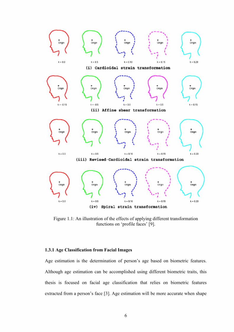
transformation functions that were studied in relevance to facial growth. Figure 1.1

illustrates the effects of these four transformation functions.

6

Figure 1.1: An illustration of the effects of applying different transformation functions on ‘profile faces’ [9].

1.3.1 Age Classification from Facial Images

Age estimation is the determination of person’s age based on biometric features.

Although age estimation can be accomplished using different biometric traits, this

thesis is focused on facial age classification that relies on biometric features

extracted from a person’s face [3]. Age estimation will be more accurate when shape

7

and skin features are taken into consideration. The basis of this thesis is a statistical

analysis of facial features in order to classify the facial images according to

corresponding age intervals.

1.4 The Work Done In This Study

In this study supervised learning is used to train the computer with a specific number

of training facial images. The relationship between the coded representation of the

training faces’ ages and the actual ages of the test subjects is then learnt. Once this

relationship is established, it is possible to estimate the age of a previously unseen

image. Regarding to this issue shape variation analysis is done by categorizing the

differences between ratios during formative years, in order to classify the facial

images, texture analysis is applied on female and male facial images separately by

four different techniques namely LBP (Local Binary Pattern) and mPCA (modular

Principal Component Analysis) as subpattern-based approaches, and, PCA

(Principal Component Analysis) and ssLDA (subspace Linear Discriminant

Analysis) as holistic methods (the process of applying one of the various algorithms

to the whole-face) are used as feature extractors with the combination of the

preprocessing techniques of histogram equalization (HE) and mean-and-variance

normalization (MVN) in order to minimize the effect of illumination.

The success and popularity of these algorithms are mainly due to their statistics-

based ability of automatically deriving the features instead of relying on humans for

their definitions. These algorithms are widely studied for the recognition and

classification of human beings. Although these feature extraction algorithms are

successful, they are not perfect as there are many obstacles such as changes in

illumination, pose, facial expression, facial texture (e.g. wrinkles), and shape (e.g.

8

weight gain or loss), facial hair, presence of partial occlusions (e.g. glasses, scarf)

and age progression [10] as shown in Figures 1.2 through 1.8.

Figure 1.2: Difference in Illumination (a) Brighter image (b) Darker image

Figure 1.3: Difference in Pose (a) Frontal image (b) Profile image with some angle.

Figure 1.4: Difference in Facial Expression (a) Angry Face (b) Happy Face.

9

Figure 1.5: Difference in Facial Texture (a) Image without wrinkles (b) Image with wrinkles.

Figure 1.6: Difference in Facial Texture (a) Normal Face (b) Makeup Face

Figure 1.7: Difference in Facial Hair (a) Face without mustache and beard (b) Face

with mustache and beard.

Figure 1.8: Presence of Partial Occlusions (a) Face without glasses (b) Face with

glasses.

The holistic and subpattern-based approaches are implemented using the cropped

face images from two different datasets selected from MORPH [30] and FG-NET

[29] databases. Various experiments are performed to test the classification

performance of the LBP, mPCA, original PCA, subspace LDA approaches. The

results are presented in the further sections. The accuracy of age classification of

10

female and male are compared with the four methods mentioned above. Finally in

order to decrease the age range interval, the second step of classification is done right

after the first step of classification.

The rest of the thesis is organized as follows. Chapter 2 presents the preprocessing

steps to prepare images for training and testing phases. In Chapter 3, the methods

used for facial feature extraction are discussed. Chapter 4 presents the geometric

variation on face images across age progression. The experimental results for age

classification on female and male facial images are demonstrated in Chapter 5.

Finally, Chapter 6 presents the conclusions.

11

Chapter 2

PREPROCCESSING

Images of subjects captured by camera will normally be out of phase with each other

because of difference in background, pose of head, contrast of images, number of

intensity levels, size of the images and other causes. Most of the programs cannot

automatically solve all of these problems. Therefore some of the deficiencies of these

images should be solved before defining them to the program as input and some of

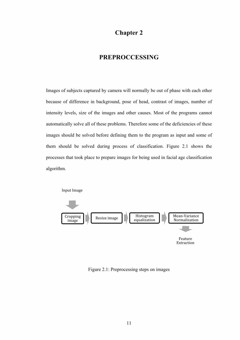
them should be solved during process of classification. Figure 2.1 shows the

processes that took place to prepare images for being used in facial age classification

algorithm.

Figure 2.1: Preprocessing steps on images

Input Image

Cropping image Resize image Histogram

equalization Mean‐Variance Normalization

Feature Extraction

12

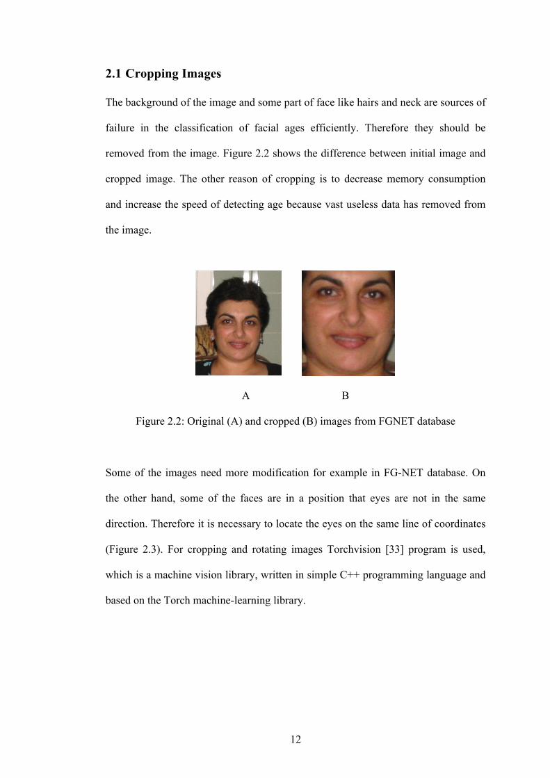
2.1 Cropping Images

The background of the image and some part of face like hairs and neck are sources of

failure in the classification of facial ages efficiently. Therefore they should be

removed from the image. Figure 2.2 shows the difference between initial image and

cropped image. The other reason of cropping is to decrease memory consumption

and increase the speed of detecting age because vast useless data has removed from

the image.

A B

Figure 2.2: Original (A) and cropped (B) images from FGNET database

Some of the images need more modification for example in FG-NET database. On

the other hand, some of the faces are in a position that eyes are not in the same

direction. Therefore it is necessary to locate the eyes on the same line of coordinates

(Figure 2.3). For cropping and rotating images Torchvision [33] program is used,

which is a machine vision library, written in simple C++ programming language and

based on the Torch machine-learning library.

13

Figure 2.3: Original and rotated image

2.2 Resizing and Interpolation of Images

Each image that is given to the algorithm as an input may have different size

therefore in this step it is necessary to unify size of all images. In our work, in order

to resize the images, interpolation techniques had been used. Interpolation means

resizing images by using known data to estimate values at known location. There are

three types of interpolation such as nearest neighbor interpolation, bilinear

interpolation and bicubic interpolation. In this thesis, bicubic interpolation which is

the most efficient method among interpolation techniques has been used. Bicubic

interpolation uses 16 nearest neighbors of new location to estimate the intensity level

of it. Bicubic interpolation preserves detail of image better than the other

interpolation methods.

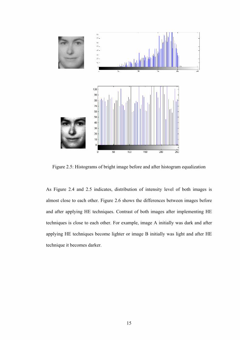
2.3 Histogram Equalization

Histogram in image processing represents the relative frequency of occurrence of

various gray levels in the image. Images may have different number of intensity

levels, congestion of intensities in different levels might be different and these

differences among images will decrease the efficiency of facial age classification.

In the same database the intensity levels of two images might be different. In order to

distribute their levels of intensities, histogram equalization (HE) technique can be

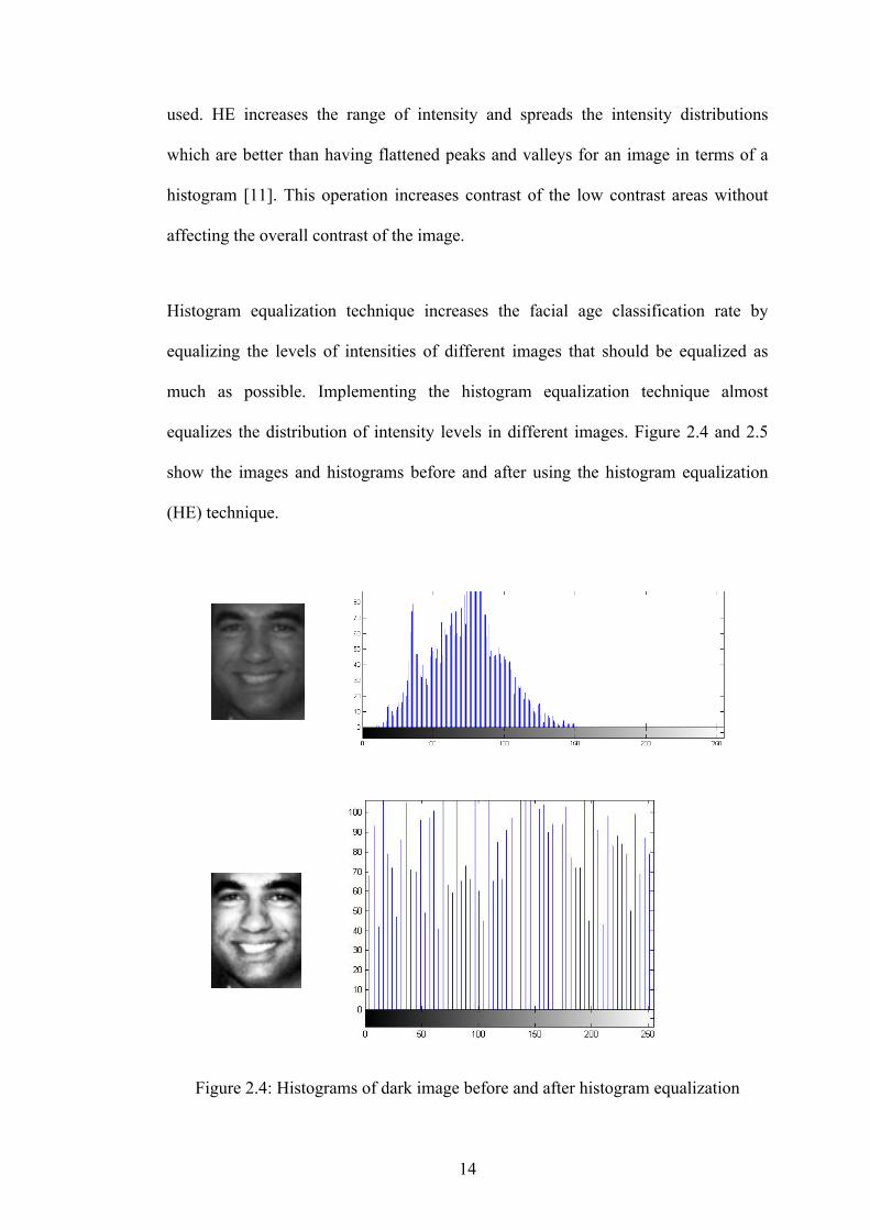
14

used. HE increases the range of intensity and spreads the intensity distributions

which are better than having flattened peaks and valleys for an image in terms of a

histogram [11]. This operation increases contrast of the low contrast areas without

affecting the overall contrast of the image.

Histogram equalization technique increases the facial age classification rate by

equalizing the levels of intensities of different images that should be equalized as

much as possible. Implementing the histogram equalization technique almost

equalizes the distribution of intensity levels in different images. Figure 2.4 and 2.5

show the images and histograms before and after using the histogram equalization

(HE) technique.

Figure 2.4: Histograms of dark image before and after histogram equalization

15

Figure 2.5: Histograms of bright image before and after histogram equalization

As Figure 2.4 and 2.5 indicates, distribution of intensity level of both images is

almost close to each other. Figure 2.6 shows the differences between images before

and after applying HE techniques. Contrast of both images after implementing HE

techniques is close to each other. For example, image A initially was dark and after

applying HE techniques become lighter or image B initially was light and after HE

technique it becomes darker.

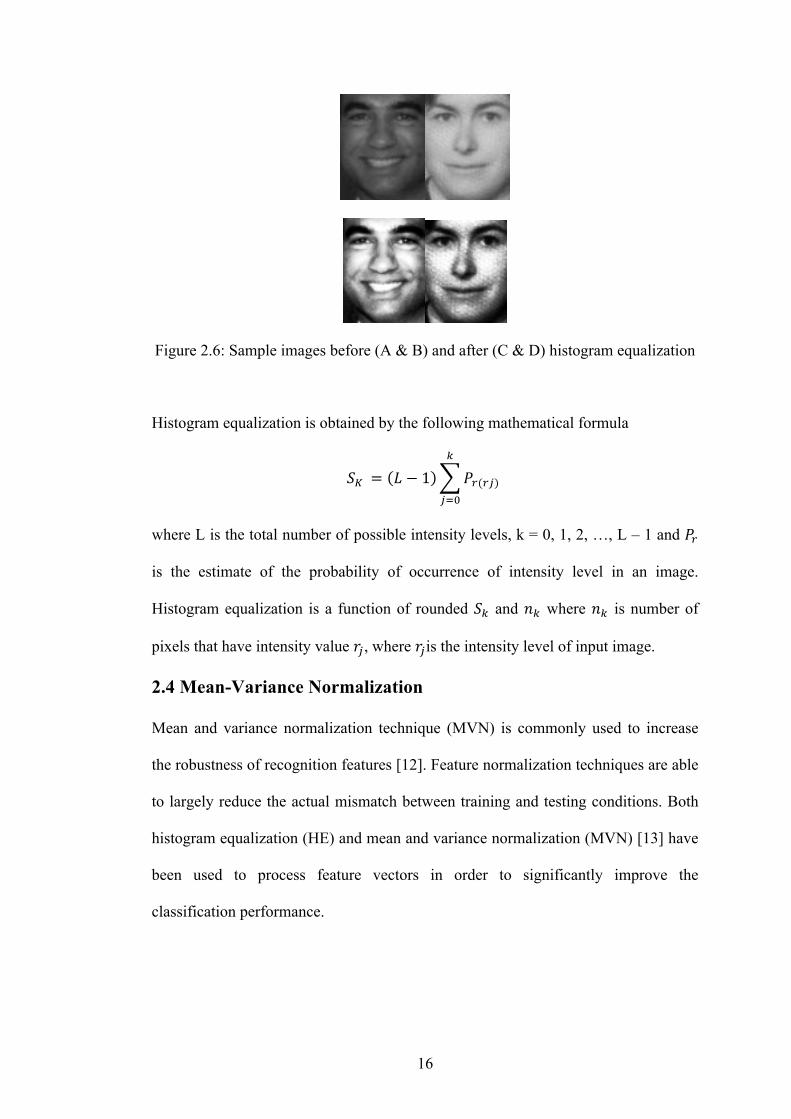
16

Figure 2.6: Sample images before (A & B) and after (C & D) histogram equalization

Histogram equalization is obtained by the following mathematical formula

𝑆! = 𝐿 − 1 𝑃!(!")

!

!!!

where L is the total number of possible intensity levels, k = 0, 1, 2, …, L – 1 and 𝑃!

is the estimate of the probability of occurrence of intensity level in an image.

Histogram equalization is a function of rounded 𝑆! and 𝑛! where 𝑛! is number of

pixels that have intensity value 𝑟!, where 𝑟!is the intensity level of input image.

2.4 Mean-Variance Normalization

Mean and variance normalization technique (MVN) is commonly used to increase

the robustness of recognition features [12]. Feature normalization techniques are able

to largely reduce the actual mismatch between training and testing conditions. Both

histogram equalization (HE) and mean and variance normalization (MVN) [13] have

been used to process feature vectors in order to significantly improve the

classification performance.

17

MVN is obtained as follows:

R = X – 𝑀! , MVN = R / std (R)

where X is a matrix consisting of the intensity values of a grayscale image, 𝑀!is

mean value of X and std is standard deviation of R.

In the study, after these steps are done, preprocessing on the facial images were

finished and the images become ready to enter into training and testing parts of the

feature extraction techniques (LBP, mPCA, PCA and ssLDA), which will be

explained in the next chapter.

18

Chapter 3

FEATURE EXTRACTION

Adult faces contain lots of wrinkles and other skin artifacts known as face features

which are the essential component of a successful biometrics classification

algorithm; therefore accuracy of feature extraction is important to detect the age of

facial image. For this purpose, facial images are used for the classification of age

groups and the classification is done using Local Binary Patterns (LBP), modular

Principal Component Analysis (mPCA), Principal component analysis (PCA) and

subspace Linear Discriminant Analysis (ssLDA) statistical approaches for texture

analysis.

One way to achieve the texture classification in gray scale images is to use the LBP

texture descriptors to build several local descriptions of the facial image and

concatenate them into a global description. The LBP operator [14] is one of the best

performing texture descriptors and it has been widely used in various applications.

The rational behind mPCA is same as rational behind LBP, face images were divided

into smaller regions in mPCA and LBP, the difference is the weight vectors that are

computed for each of these regions. The weights are more representative of the local

information of the face in mPCA while LBP concerns the binary number of each

region and the histogram of the labels can be used as a texture descriptor for each

region. These local feature based methods are more robust against variations in pose

19

or illumination than holistic methods. Holistic description of a face is not reasonable

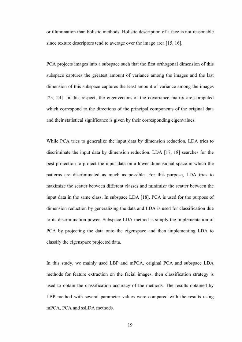
since texture descriptors tend to average over the image area [15, 16].

PCA projects images into a subspace such that the first orthogonal dimension of this

subspace captures the greatest amount of variance among the images and the last

dimension of this subspace captures the least amount of variance among the images

[23, 24]. In this respect, the eigenvectors of the covariance matrix are computed

which correspond to the directions of the principal components of the original data

and their statistical significance is given by their corresponding eigenvalues.

While PCA tries to generalize the input data by dimension reduction, LDA tries to

discriminate the input data by dimension reduction. LDA [17, 18] searches for the

best projection to project the input data on a lower dimensional space in which the

patterns are discriminated as much as possible. For this purpose, LDA tries to

maximize the scatter between different classes and minimize the scatter between the

input data in the same class. In subspace LDA [18], PCA is used for the purpose of

dimension reduction by generalizing the data and LDA is used for classification due

to its discrimination power. Subspace LDA method is simply the implementation of

PCA by projecting the data onto the eigenspace and then implementing LDA to

classify the eigenspace projected data.

In this study, we mainly used LBP and mPCA, original PCA and subspace LDA

methods for feature extraction on the facial images, then classification strategy is

used to obtain the classification accuracy of the methods. The results obtained by

LBP method with several parameter values were compared with the results using

mPCA, PCA and ssLDA methods.

20

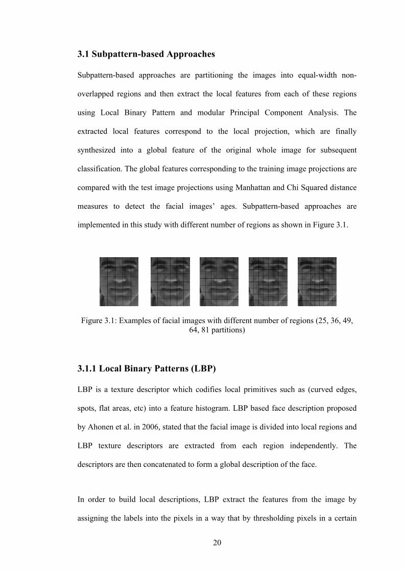
3.1 Subpattern-based Approaches

Subpattern-based approaches are partitioning the images into equal-width non-

overlapped regions and then extract the local features from each of these regions

using Local Binary Pattern and modular Principal Component Analysis. The

extracted local features correspond to the local projection, which are finally

synthesized into a global feature of the original whole image for subsequent

classification. The global features corresponding to the training image projections are

compared with the test image projections using Manhattan and Chi Squared distance

measures to detect the facial images’ ages. Subpattern-based approaches are

implemented in this study with different number of regions as shown in Figure 3.1.

Figure 3.1: Examples of facial images with different number of regions (25, 36, 49, 64, 81 partitions)

3.1.1 Local Binary Patterns (LBP)

LBP is a texture descriptor which codifies local primitives such as (curved edges,

spots, flat areas, etc) into a feature histogram. LBP based face description proposed

by Ahonen et al. in 2006, stated that the facial image is divided into local regions and

LBP texture descriptors are extracted from each region independently. The

descriptors are then concatenated to form a global description of the face.

In order to build local descriptions, LBP extract the features from the image by

assigning the labels into the pixels in a way that by thresholding pixels in a certain

21

neighborhood with the center value. LBP construct the code for every pixel and

considers the result as a binary number. The occurrence histogram of these labels is

used as texture features or descriptors. Finally different histograms can be combined

as a code image.

To be able to deal with textures at different scales, the LBP operator was later

extended to use neighborhoods of different sizes [16]. A circular neighborhood and

bilinearly interpolating values at non-integer pixel coordinates allow any radius and

number of pixels in the neighborhood. Figure.3.2 demonstrates an example of

circular neighborhoods.

a) p = 8, r = 1 b) p = 16, r = 2 c) p = 8, r = 2

Figure 3.2: Example of circular neighborhoods.

3.1.1.1 Local Binary Patterns (LBP) Algorithm

Three different levels of locality can be applied to have a description of the face:

The LBP labels for the histogram contain information about the patterns on a pixel-

level, the labels are summed over a small region to produce information on a regional

level; the regional histograms are concatenated to build a global description of the

face [15].

22

The LBP code construction steps for every pixel are as follows:

Step 1: assume that the image size is 64x80 pixels (metrics contains the pixel values

of 64 rows and 80 columns), in order to divide the image into regions. At first, if 5*5

is the number of selected regions, the image should be divisible by 5, after resizing

the image (resized image size is 60x80), then it is ready to split the image into 5*5

blocks so that each region contains 12*16 pixels. In Figure 3.1, different number of

rectangular regions are demonstrated. The regions do not need to be rectangular or

cover the whole image part, but it can be circular region which located in fiducial

points as shown in Figure.3.2.

Step 2: Block processing will apply on each region separately. It is needed to assign

the label to each pixel in corresponding region. Center pixel, number of neighbor

pixels and radius of region are defined. If the pixel value of neighbors are bigger than

the center pixel value, the label is 1; otherwise it is 0. So that each pixel of the region

is labeled as

𝐿𝐵𝑃 !,! 𝑋! = 𝑢(𝑋! − 𝑋!!!!! )2! (3.1)

𝑢! =1, 𝑦 ≥ 00, 𝑦 < 0

where 𝑋! is the pixel value of center point, 𝑋! pixel value of sample point. The

notation (p,r) will be used for pixel neighborhoods where p is the number of

sampling points on a circle of radius of r. The calculation is depicted graphically in

Figures 3.3 and 3.4

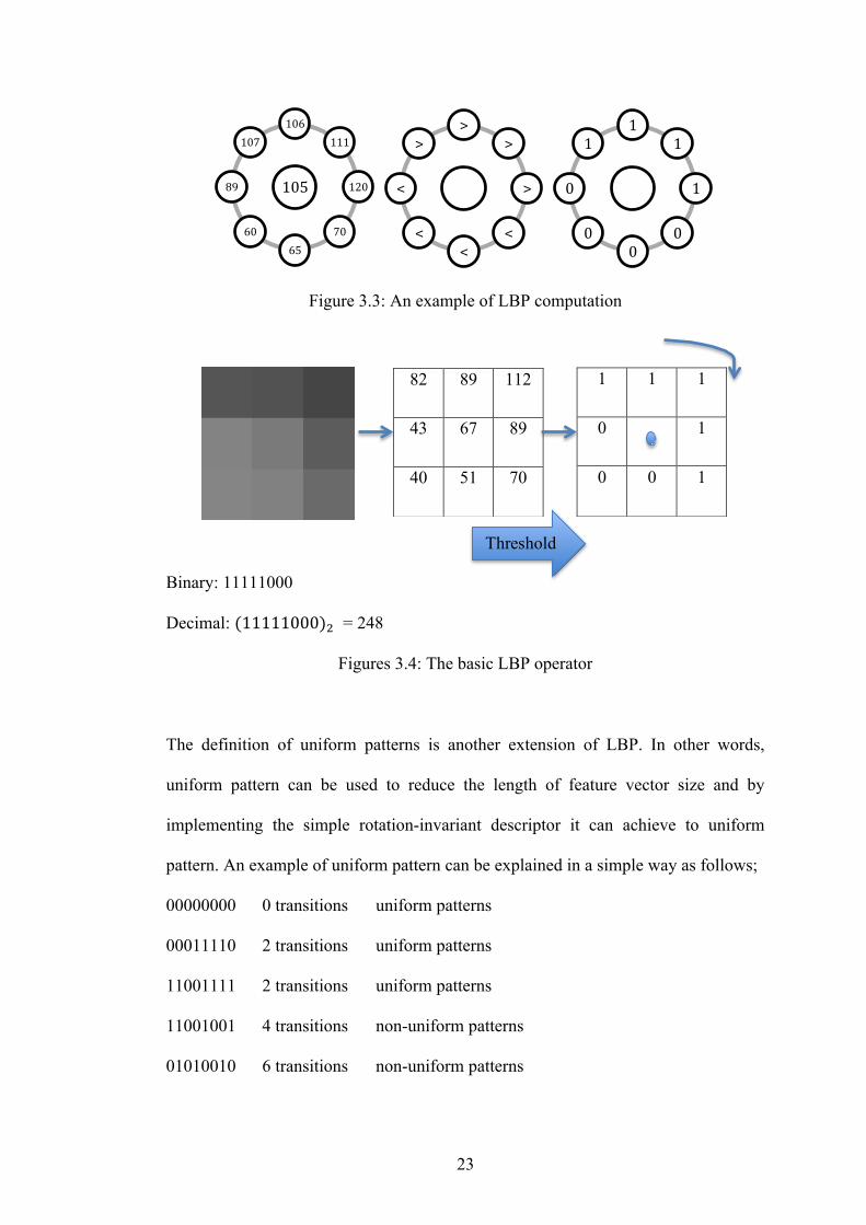
23

Figure 3.3: An example of LBP computation

Figure.3.6

Binary: 11111000

Decimal: (11111000)! = 248

Figures 3.4: The basic LBP operator

The definition of uniform patterns is another extension of LBP. In other words,

uniform pattern can be used to reduce the length of feature vector size and by

implementing the simple rotation-invariant descriptor it can achieve to uniform

pattern. An example of uniform pattern can be explained in a simple way as follows;

00000000 0 transitions uniform patterns



11001001 4 transitions non-uniform patterns

01010010 6 transitions non-uniform patterns

105

106 111

120

70 65

60

89

107

> >

>

< <

<

<

>

1 1

1

0 0

0

0

1

1 1 1

0 1

0 0 1

82 89 112

43 67 89

40 51 70

Threshold

24

Step3: Spatially enhanced histogram is needed in order to obtain LBP histogram. In

the spatially enhanced histogram, the LBP labels for the histogram contain

information about the patterns on a pixel-level which is explained in step 2. The

labels are summed over a region to produce information on a regional level, and each

region has a histogram itself so histograms are concatenated to build a global

description of the face. Therefore, LBP histogram can be used as a texture descriptor.

Figure 3.5 shows samples of enhanced histogram of image and image code before

and after applying LBP is depicted in Figure 3.6.

Figure 3.5: Histogram of image after concatenating all histograms

a b

Figure 3.6: a) Original Image, b) LBP Image

In this thesis we used Local Binary Patterns (LBP) histograms and Chi Square as

dissimilarity measure to find the system classification.

Chi Square distance [19] is a metric in which the distance between two vectors is

25

𝐷(!, !) = 𝜒! = 𝑥! − 𝑦! !

𝑥! + 𝑦!

!

!!!

where X and Y are vectors of length n.

3.1.2 Modular Principal Component Analysis (mPCA)

Modular PCA method is an extension of the conventional PCA method. In modular

Principle Component Analysis (mPCA), an image is first partitioned into several

smaller regions and the weight vectors are computed for each of these regions which

will be more representative of the local information. Then a single conventional PCA

is applied to each of these regions, and therefore, the variations in the image, such as

illumination and pose variations, will only affect some regions in mPCA rather than

the whole image in PCA [20]. In other word, modular Principal Component Analysis

(mPCA) overcomes the difficulties of regular PCA. Generally, conventional PCA

considers the global information of each image and represents them with a set of

weights. Under these conditions the weight vectors will vary considerably from the

weight vectors of the images with normal pose and illumination, hence it is difficult

to identify them correctly. On the other hand, mPCA method applies PCA on smaller

regions and the weight vectors are calculated for each of them, so local information

of the image can show the weights better and for variation in the pose or

illumination, only some of the regions will vary and the rest of the regions will

remain the same as the regions of a normal image [21].

3.1.2.1 Modular Principal Component Analysis (mPCA) Algorithm

The first step of image classification by mPCA algorithm [21] after collecting Ii

images (Ii= [I1, I2…, IM]) is dividing each image in the training set into N smaller

images. The average image of all the training sub-images is calculated using equation

(3.2). Equation (3.3) shows normalizing each training sub-image by subtracting it

26

from the mean. Then covariance matrix can be computed from the normalized sub-

images using equation (3.4). Finding the eigenvectors 𝐸!, 𝐸!,… ,𝐸!! of covariance

matrix that are associated with the 𝑀! largest eigenvalues is the next step in which

the eigenvectors according to their corresponding eigenvalues from high to low are

ordered. Then the projection of training sub-images is computed in equation (3-5)

using the eigenvectors.

𝐴 = !!.!

𝐼!"!!!!

!!!! (3.2)

𝑌!" = 𝐼!" − 𝐴 ∀!,! (3.3)

𝐶 = !!.!

𝑌!" .𝑌!"!!!!!

!!!! (3.4)

𝑊!"#$ = 𝐸!! . 𝐼!"# − 𝐴 ∀!,!,!,! (3.5)

The last step of classifying images by mPCA algorithm is finding the projection for

the test sub-images into the same eigenspace according to equation (3.6). The

projected test sub-image is compared to every projected training sub-image and the

training image that is found to be closest to the test image is used to identify the

training image.

𝑊!"#!$% = 𝐸!! . 𝐼!"#!$ − 𝐴 ∀!,! (3.6)

3.2 Holistic Approaches

Holistic or appearance based approaches deal with the entire image, not some

specific features or some smaller parts. While analyzing the whole face, it tries to

match templates and with the global representations, it is aimed to identify faces

[22]. To take the whole image as one, and work on it means the following; there will

be only one matrix with one dimension composed of all pixels in the image and all

the information in the image will be kept and processed. This can be both

27

advantageous and disadvantageous. It is our benefit to have any information about

the person to discriminate them from the others, where in a feature-based approach

this is not possible, but also there may be unwanted data in the image like a wall, tree

or some other items’ parts rather than person’s face in the background of an image. If

the second case is present, of course this will affect the performance of the face

classification system. As an example, in Figure 3.7-a, there are no background items,

after cropping the whole face, every pixel will be useful to discriminate from others;

but in Figure 3.7-b,c,d, we have some items like checked surface near the cheek, and

also the part of a shirt on the bottom, which will be analyzed as well during the

process of classification and will mislead the algorithm that is used.

a b c d

Figure 3.7: Samples of cropped facial images

A one-dimensional matrix composed of every pixel of the image, can be huge in size,

so it is hard to be analyzed by a machine. The two popular statistical dimensionality

reduction methods, PCA and subspace LDA can be used in a holistic manner, where

they extract features from the whole face image, reduce the size and then classify

them accordingly again considering the whole image.

For this purpose, statistical dimensionality reduction methods such as Principal

Component Analysis (PCA) and Linear Discriminant Analysis (LDA) are

28

demonstrated to be successful in several academic studies and commercial

applications. The success and popularity of these algorithms are mainly due to their

statistics-based ability of automatically deriving the features instead of relying on

humans for their definitions. In the next two sections PCA and subspace LDA

methods are explained in detail.

3.2.1 Principal Component Analysis (PCA)

Principal Component Analysis (PCA) [23] is one of the most common techniques to

reduce the number of dimensionality, which makes this in a very efficient way,

making PCA successful and popular. PCA is efficient, because the algorithm

achieves its job with only a simple linear algebra and without much loss in the data.

Before describing the PCA, it is important to define eigenvectors in mathematical

terms as it is important part of this algorithm. The mathematical definition of

eigenvector can be defined as AC=C, where A is a square matrix, C is the eigenvector

of A and it is not a zero vector, and real or complex must be present. Eigenvectors

can be only found for square matrices but not every square matrix has them. And if it

does, and the square matrix has the dimension m x m, then there are m eigenvectors.

The important property of eigenvector is that when we multiply it with a vector, it

only makes it longer; it does not change its direction.

When we reconsider PCA with mathematical terms, we can say that it projects

images into a subspace such that the first orthogonal dimension of this subspace

captures the greatest amount of variance among the images and the last dimension of

this subspace captures the least amount of variance among the images [23, 24, 25]. In

this respect, the eigenvectors of the covariance matrix are computed which

29

correspond to the directions of the principal components of the original data and their

statistical significance is given by their corresponding eigenvalues.

3.2.1.1 Principal Component Analysis (PCA) Algorithm

The PCA algorithm can be stated as follows;

Step 1: Take the all images (xi) into a row of vectors of size V: xi = [xi1 … xi v],

where V is the total numbers of pixels in an image.

Step 2: Subtract the Mean: Calculate the mean m, which equals sum of all training

images divided by the number of them, and subtract it from of x;

𝑚 = 𝑥 !!!!! ∗ 1/𝑁 (3.7)

𝑦! = 𝑥! −𝑚 (3.8)

Step 3: Create the data matrix by combining the above vectors; 𝑍 = 𝑦!! …𝑦!!

Step 4: Calculate the covariance matrix:

𝐶 = 𝑍𝑍! (3.9)

Step 5: Determine the eigenvalues of covariance matrix C.

Step 6: Sort the eigenvalues (and corresponding eigenvectors) in decreasing order.

Step 7: Assume that N ≤ V, select the first d ≤ R eigenvectors and generate the

dataset in the new representation.

Step 8: Compare the test image’s projection matrix with the projection matrix of

each training image by using a similarity measure. The result is the training image

which is the closest to the test image.

3.2.2 Subspace Linear Discriminant Analysis (ssLDA)

Linear Discriminant Analysis [24] is a method that in which statistical and

supervised machine learning techniques are used to classify the unknown classes in

test sample based on known classes in training samples. LDA is used to project the

samples from the high dimensional space to a lower dimensional feature space.

30

Maximize between class variance and minimize the within class variance are the

aims of LDA to find the most discriminant projection direction. Figure.3.8 shows an

example of 3 age intervals classified using LDA.

In this study, for the first step of classification, 3 classes are defined in 3 age

intervals as 0-20, 21-40 and 41-60 as shown in Figure 3.8. The first row images

belong to 0 to 20 years old, second row images belong to 21 to 40 and third row

images belong to 41 to 60 years old human beings. Large variance between classes

and small variance within classes is obvious.

Figure 3.8: Facial images of three different age intervals selected from FG-NET aging database

Subspace LDA method is simply the implementation of PCA by projecting the data

onto the eigenspace and then implementing LDA to classify the eigenspace projected

data. Within class scatter matrix measures the amount of scatter between items in the

same class. For the ith class, a scatter matrix (Si) is calculated as the sum of the

covariance matrices of the centered images in that class as follows

𝑆! = 𝑥 − 𝑚! 𝑥 − 𝑚!!

!∈!! (3.10)

31

where 𝑚! is the mean of the images in the class. The within class scatter matrix (𝑆!)

is the sum of all the scatter matrices. Here 𝑋!is the projection constructed from PCA

algorithm. 𝑆!is calculated as

𝑆! = 𝑆!!!!! (3.11)

where L is the number of classes.

Equation (3.12) shows the between classes scatter matrix (𝑆!) which measures the

amount of scatter between classes. It is calculated as the sum of the covariance

matrices of the difference between the total mean and the mean of each class as

follows

𝑆! = 𝑛! 𝑚! −𝑚 𝑚! −𝑚 !!!!! (3.12)

where 𝑛! is the number of images in the class, 𝑚!is the mean of the images in the

class and 𝑚 is the mean of all the images.

3.2.2.1 Subspace Linear Discriminent Analysis (ssLDA) Algorithm

Subspace Linear Discriminant Analysis (ssLDA) algorithm can be stated as follows:

Step 1: Take all the images (𝑥!) into a row vector of size V: 𝑥! = 𝑥!! … 𝑥!!

Step 2: Subtract the Mean: Calculate the mean m, which equals sum of all training

images divided by the number of them, and subtract it from all the images (x);

𝑚 = 𝑥!!!!! ∗ 1/𝑁 (3.13)

𝑦! = 𝑥! − 𝑚 (3.14)

Step 3: Create the data matrix by combining the above vectors; Z = 𝑦!! …𝑦!!

Step 4: Calculate the covariance matrix:

C = 𝑍𝑍! (3.15)

Step 5: Determine the eigenvalues of covariance matrix C

Step 6: Sort the eigenvalues (and corresponding eigenvectors) in decreasing order.

32

Step 7: Assume that N ≤ V, select the first d ≤ R eigenvectors and generate the

dataset in the new representation.

Step 8: Take the projection from the PCA as an input to LDA, Xi

Step 9: Calculate within-class scatter matrix, 𝑆! of X.

Step 10: Calculate between-class scatter matrix, 𝑆!.

Step 11: Calculate the eigenvectors of the projection matrix:

𝑊 = 𝑒𝑖𝑔 𝑆!!! 𝑆! (3.16)

Step 12: Compare the test image’s projection matrix with the projection matrix of

each training image by using a similarity measure. The result is the training image

which is the closest to the test image.

In this study the Manhattan distance is used for PCA and ssLDA as similarity

measure. Manhattan Distance is a metric in which the distance between two points is

the sum of the (absolute) differences of their coordinates. It is also known as

rectilinear distance, L1 distance or city block distance.

The Manhattan distance between the point P1 with coordinates (x1; y1) and the point

P2 at (x2; y2) is:

𝐷!"#!!""!# = 𝑥! − 𝑥! + 𝑦! − 𝑦!

and Manhattan distance between two vectors X, Y of length n is [19]:

𝐷 !, ! = 𝑥! − 𝑦!

!

!!!

33

Chapter 4

GEOMETRY ANALYSIS

4.1 Geometric Variation

Age estimates are obtained from faces whose shape and degree of skin wrinkling are

changed. Both of the variables affect the perceived age of faces. [26]. Therefore,

focus on the contributions of shape-based features and texture-based features in age

estimation or classification from facial images is needed. Facial shape variations are

more visible during babyhoods, on the other hand it becomes subtle during

adulthood. Hence, facial aging can be described as a problem of characterizing facial

shape and facial texture as functions of time [8].

Infant faces have lots of wrinkles and it is not suitable to just extract the texture

features of babies but since the structure of head bones in infanthood is not full-

grown and the ratios between primary features (e.g. distance between eyes, face

width, length, thickness of nose, etc.) are different from those in other life periods,

using the geometric relations of primary features is more reliable than wrinkles when

an image is judged to be a baby or not.

In this thesis, LBP, mPCA, PCA and ssLDA operators are used for texture analysis

as it is discussed before in chapter 3. In this chapter the geometric features of facial

images and geometric variation in babies versus adults are considered. In Figure 4.1,

the variation of distance between primary features from childhood to adulthood is

demonstrated.

34

a: 2 years old, b: 16 years old, c: 29 years old

a: 1 years old, b: 22 years old, c: 45 years old

Figure 4.1: Variation of distance between primary features

4.2 Ratio Analysis

Kwon and Lobo [2] classified ages from facial images into 3 age groups as babies,

young adults and senior adults. They used cranio-facial development theory and skin

wrinkle analysis in their study. Using the primary features of the human face such as

eyes, nose, mouth, chin and virtual top of the head; mainly 6 different ratios are

calculated to distinguish babies from young adults and senior adults. Then they used

secondary feature analysis with a wrinkle geography map to detect and measure

wrinkles to distinguish seniors from babies and young adults. Finally, they combined

ratios and wrinkle information obtained from facial images to classify faces into 3

age groups.

From these primary features, geometric ratios are computed. Figure 4.2 graphically

explains these ratios.

35

Figure 4.2: Six different ratios [2].

In babyhood, the head is near a circle. The distance from eyes to mouth is close to

that between two eyes. With the growth of the head bone, the head becomes oval,

and the distance from the eyes to the mouth becomes longer. Besides, the ratio of the

distance between babies’ eyes and noses and that between noses and mouths is close

to one, while that of adults’ is larger than one, as illustrated in Figures 4.1 (a) and (b,

c). Therefore, two geometric features are defined below for recognizing babies.

4.2.1 Algorithm Using Ratio Analysis

The algorithm is as follows:

Step 1: Locating the primary features is very important step in extraction of features,

and it can be automatically or manually. Wen-Bing Horng et. al [27] automatically

located the primary features in their study. First of all central horizontal line of the

image is found, then they found the eyes location, and finally nose and mouth

36

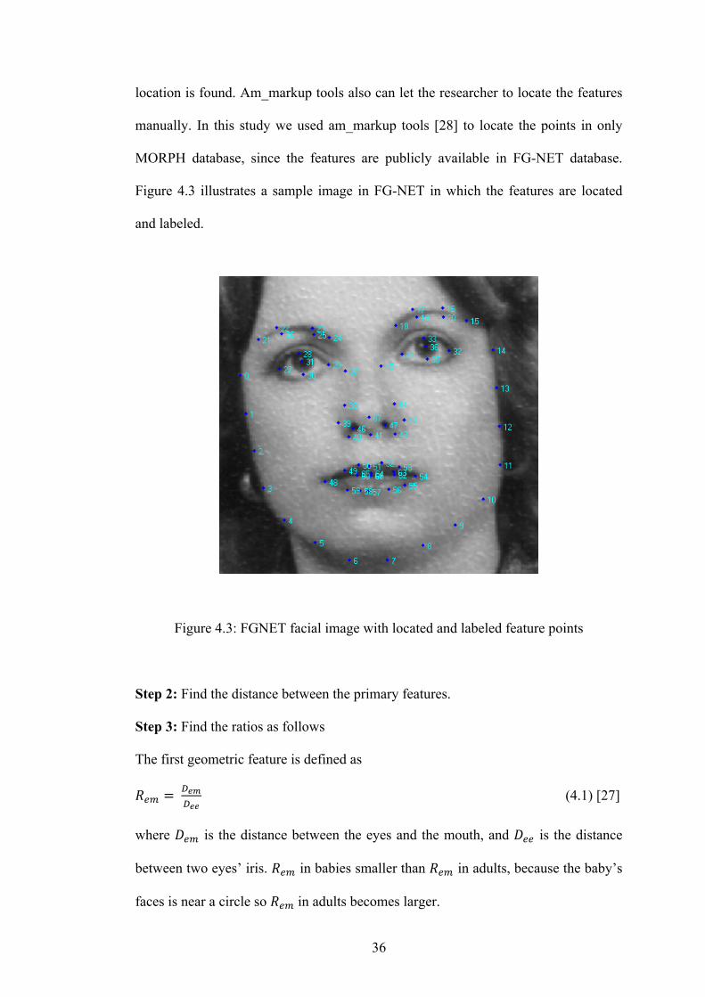
location is found. Am_markup tools also can let the researcher to locate the features

manually. In this study we used am_markup tools [28] to locate the points in only

MORPH database, since the features are publicly available in FG-NET database.

Figure 4.3 illustrates a sample image in FG-NET in which the features are located

and labeled.

Figure 4.3: FGNET facial image with located and labeled feature points

Step 2: Find the distance between the primary features.

Step 3: Find the ratios as follows

The first geometric feature is defined as

𝑅!" = !!"!!!

(4.1) [27]

where 𝐷!" is the distance between the eyes and the mouth, and 𝐷!! is the distance

between two eyes’ iris. 𝑅!" in babies smaller than 𝑅!" in adults, because the baby’s

faces is near a circle so 𝑅!" in adults becomes larger.

37

Second geometric feature is

𝑅!"# = !!"!!"

(4.2) [27]

where 𝐷!" is the distance between the eyes and the nose, and 𝐷!" is the distance

between the nose and the mouth. The distance between the eyes and the nose of a

baby is smaller than the distance between the eyes and the nose of an adult, so the

value of 𝑅!"# becomes larger in adult faces. The values of these two ratios are used

to recognize babies in the experiments on the next chapter.

38

Chapter 5

EXPERIMENTS AND RESULTS

Together with preprocessing techniques, holistic and subpattern-based approaches

are used to classify the ages via facial images. The experiments are performed using

FGNET [29] and MORPH [30] aging databases in three different categories for

evaluating the performance of subpattern-based approaches (LBP and mPCA) and

holistic approaches (PCA and ssLDA).

In the experiments for the holistic approaches, all the training and test images used

are cropped and scaled down to 64x80 pixels from the original sizes, so that they

only include the head of the individuals that is explained in detail in Chapter 2. For

the subpattern-based approaches, in order to divide the images to equal size with

proper values, the images are resized to 78x63, 80x60, 78x60, 77x63, 72x63, 80x60,

77x55, 72x60 pixels for 9, 25, 36, 49, 81, 100, 121 and 144 subpatterns respectively.

Three datasets are selected from FG-NET and MORPH databases which include at

least three samples for each individual.

For the comparison of the training image and test image projections which are the

results of feature extraction algorithms, they are compared with Manhattan distance

measure and Chi squared distance measure [19] to classify the face images according

to the corresponding age. For calculating this measure, test image projections are

subtracted from the training image projections and for each person’s projection, the

39

absolute differences are summed. The smallest difference is the one found by the

algorithm which is chosen as the closest age for that test image. Classification

accuracy for a set of images is computed as the ratio of the number of images

correctly classified using holistic and subpattern-based approaches to the number of

total test images in the set.

5.1 Description of Databases

5.1.1 FG-NET Aging Database

FG-NET is a large and the publicly available aging database. FG-NET database

contains 1002 images of 82 individuals at different ages with color and grey scale

face images. The images of FG-NET display significant variability in resolution,

quality, illumination and expression since the database images are collected by

scanning the photographs of subjects found in personal collections [29]. In this study,

we used frontal images of female and male subjects with free of glasses, beard and

mustache, all samples are taken from different ages. The age differences between the

selected image samples are in the range 0 - 60 years. In this study, a subset of this

database (750 images) is selected according to the ages of subjects.

5.1.2 MORPH Aging Database

MORPH database is a longitudinal aging database which contains 1724 images of

515 subjects. There are approximately 3 images per subject with different ages.

MORPH database images include age, gender and ethnicity information. Some of the

subjects with 3 frontal images at different ages from MORPH database are selected

in this thesis to perform the experiments. The age differences between the selected

image samples are in the range 2 months - 60 years. In this study, a subset of this

database (320 images) is selected according to the ages of the images. MORPH

database images include age, gender and ethnicity information. Some of the subjects

40

with 3 frontal images at different ages from MORPH database are selected in this

study to perform the experiments. The age differences between the selected image

samples are in the range of 2 months to 60 years.

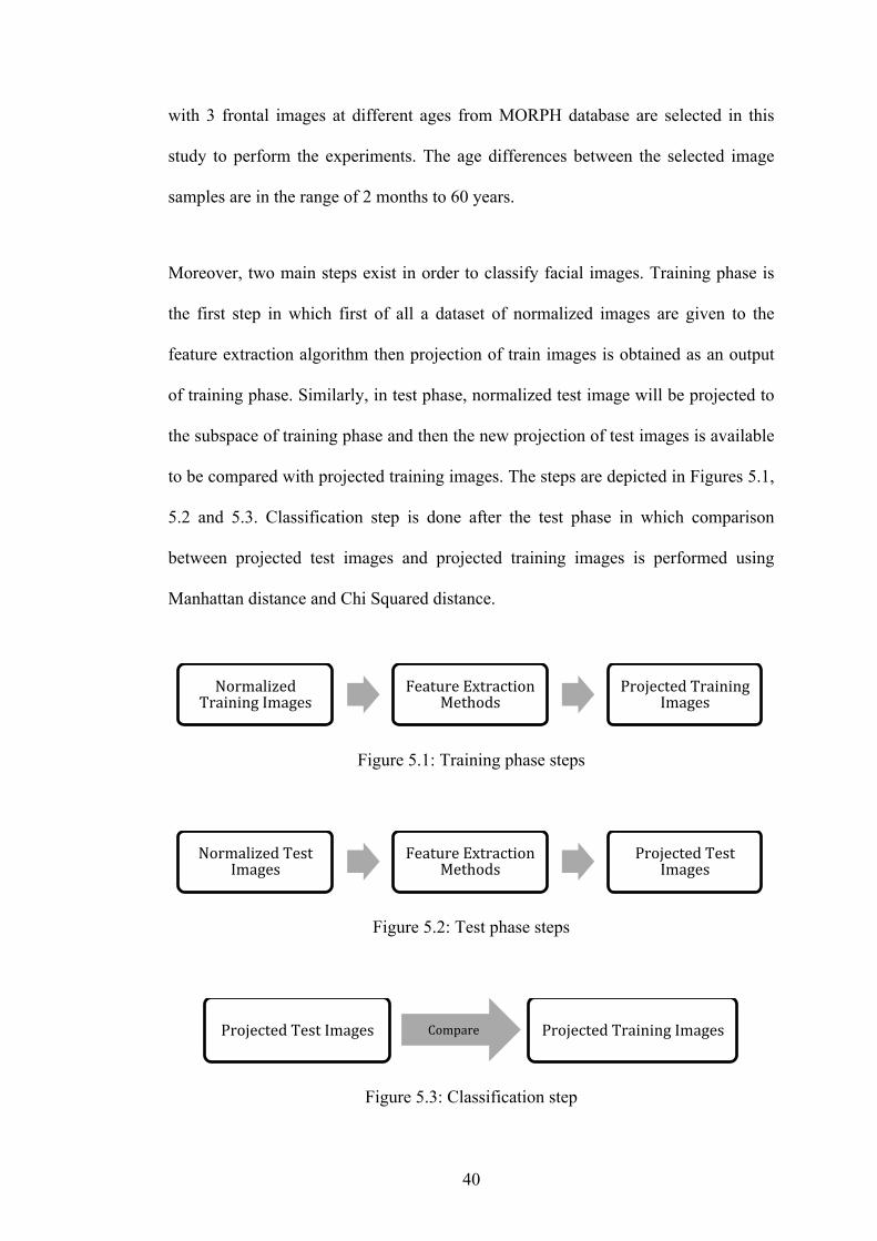
Moreover, two main steps exist in order to classify facial images. Training phase is

the first step in which first of all a dataset of normalized images are given to the

feature extraction algorithm then projection of train images is obtained as an output

of training phase. Similarly, in test phase, normalized test image will be projected to

the subspace of training phase and then the new projection of test images is available

to be compared with projected training images. The steps are depicted in Figures 5.1,

5.2 and 5.3. Classification step is done after the test phase in which comparison

between projected test images and projected training images is performed using

Manhattan distance and Chi Squared distance.

Figure 5.1: Training phase steps

Figure 5.2: Test phase steps

Figure 5.3: Classification step

Normalized Training Images

Feature Extraction Methods

Projected Training Images

Normalized Test Images

Feature Extraction Methods

Projected Test Images

Projected Test Images Compare Projected Training Images

41

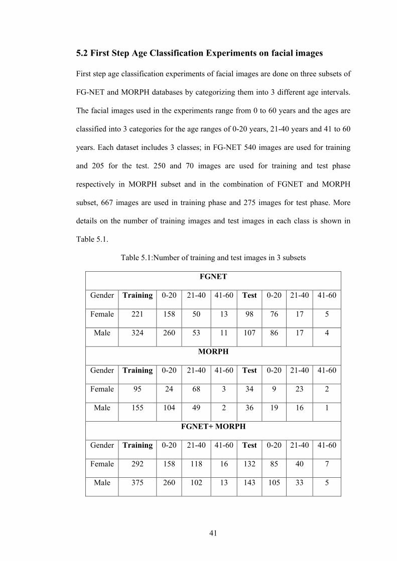
5.2 First Step Age Classification Experiments on facial images

First step age classification experiments of facial images are done on three subsets of

FG-NET and MORPH databases by categorizing them into 3 different age intervals.

The facial images used in the experiments range from 0 to 60 years and the ages are

classified into 3 categories for the age ranges of 0-20 years, 21-40 years and 41 to 60

years. Each dataset includes 3 classes; in FG-NET 540 images are used for training

and 205 for the test. 250 and 70 images are used for training and test phase

respectively in MORPH subset and in the combination of FGNET and MORPH

subset, 667 images are used in training phase and 275 images for test phase. More

details on the number of training images and test images in each class is shown in

Table 5.1.

Table 5.1:Number of training and test images in 3 subsets

FGNET

Gender Training 0-20 21-40 41-60 Test 0-20 21-40 41-60

Female 221 158 50 13 98 76 17 5

Male 324 260 53 11 107 86 17 4

MORPH


Female 95 24 68 3 34 9 23 2

Male 155 104 49 2 36 19 16 1

FGNET+ MORPH


Female 292 158 118 16 132 85 40 7

Male 375 260 102 13 143 105 33 5

42

5.2.1 Experiments Using Subpattern-based Approaches

Local Binary Pattern and Modular Principal Component Analysis are used as

subpattern-based approaches in order to classify the images according to the

corresponding ages into 3 categories. For all the tables below, the results are in (%)

for the classification rates.

5.2.1.1 Experiments Using LBP

This set of experiments is done with different subpattern sizes and neighborhood

values using LBP. The facial images from all subsets of the aging databases are

divided into 9, 16, 25, 36, 49, 64 , 81, 100, 121 and 144 subpatterns. Local Binary

Pattern histograms are extracted and concatenated into one feature histogram to

represent the whole image. Age classification using (1,8), (2,8), (1,16) and (2,16)

neighborhoods with uniform pattern is performed for female and male facial images.

The overall age classification performances for 3 different datasets of facial images

are presented in Tables 5.2-5.7. We used a nearest neighbor classifier and Chi Square

distance metrics for all LBP age classification experiments in this study.

43

Table 5.2: Female Age Classification Rates (%) with LBP on FGNET dataset

Subpattern size Neighborhood

(1,8) (2,8) (1,16) (2,16)

3x3 70.40 71.42 75.51 81.63

4x4 72.44 70.40 78.57 74.48

5x5 71.42 74.48 75.51 77.55

6x6 74.48 83.67 79.59 78.57

7x7 75.51 77.55 79.59 78.57

8x8 80.61 80.61 80.61 82.65

9x9 81.63 75.51 76.53 76.53

10x10 79.59 78.57 80.61 77.55

11x11 77.55 79.59 79.59 73.46

12x12 81.63 82.65 80.61 79.59

LBP female age classification results with different subpattern sizes and

neighborhoods are different on FGNET dataset. In addition, female age classification

results demonstrate that female age classification using 36 (6x6) subpatterns and (2,

8) neighborhoods shows better classification rate witch is 83.67%. On the other

hand, female age classification using (1, 8) neighborhood and 9 subpatterns achieves

the minimum result which is 70.40%. In other words, LBP female age classification

using 36 subpatterns and (2, 8) neighborhoods is around 13% better than female age

classification using 9 subpatterns with (1, 8) neighborhoods on FGNET dataset.

44

Table 5.3: Female Age Classification Rates (%) with LBP on MORPH dataset


(1,8) (2,8) (1,16) (2,16)

3x3 55.88 64.70 58.82 64.70

4x4 67.64 70.58 64.70 61.76

5x5 55.88 58.82 50.00 61.76

6x6 61.76 64.70 64.70 67.64

7x7 61.76 58.82 58.82 47.05

8x8 67.64 70.58 61.76 55.88

9x9 58.82 44.11 50 41.17

10x10 55.88 52.94 55.88 44.11

11x11 67.64 67.64 61.76 58.82

12x12 61.76 55.88 64.70 47.05

LBP female age classification results with different subpattern sizes and

neighborhoods are different on MORPH dataset. In addition, female age

classification results demonstrate that female age classification using 16 (4x4) and 64

(8x8) subpatterns with (2, 8) neighborhoods show better classification rate witch is

70.58 % on MORPH dataset.

45

Table 5.4: Female Age Classification Rates (%) with LBP on FGNET+MORPH dataset


(1,8) (2,8) (1,16) (2,16)

3x3 67.42 68.93 71.21 73.48

4x4 65.90 66.66 71.21 68.93

5x5 66.66 71.21 71.96 71.96

6x6 70.45 74.24 73.48 72.72

7x7 71.21 71.21 75.00 74.24

8x8 75.00 75.00 73.48 74.24

9x9 72.72 68.93 70.45 69.69

10x10 75 73.48 73.48 72.72

11x11 73.48 76.51 73.48 67.42

12x12 76.51 78.03 75.75 75.75

Similarly, the results of LBP female age classification on FGNET+ MORPH dataset

show that the maximum rate (78.03%) is obtained with 144 subpatterns and (2, 8)

neighborhoods. Moreover female age classification on FGNET is around 13% and

5% better than female age classification on MORPH and FGNET+MORPH datasets

respectively.

46

Table 5.5: Male Age Classification Rates (%) with LBP on FGNET dataset


(1,8) (2,8) (1,16) (2,16)

3x3 79.43 82.24 82.24 81.30

4x4 81.30 87.85 85.04 85.04

5x5 86.91 85.98 86.91 86.91

6x6 85.04 85.04 85.98 85.04

7x7 86.91 88.78 88.78 88.78

8x8 85.98 86.91 89.71 88.78

9x9 85.98 86.91 86.91 85.04

10x10 85.98 85.04 88.78 85.04

11x11 87.85 83.17 85.98 84.11

12x12 86.91 85.04 87.85 82.24

LBP male age classification results with different subpattern sizes and

neighborhoods are presented on FGNET dataset in Table 5.5 as shown in the table,

male age classification using 64 (8x8) subpatterns with (1, 16) neighborhoods shows

better classification rate which is 89.71%. On the other hand, male age classification

using (1, 8) neighborhood and 9 subpatterns achieves the minimum result which is

79.43%. In other words, LBP male age classification using 64 subpatterns and (1, 16)

neighborhoods is around 10% better than male age classification using 9 subpatterns

with (1, 8) neighborhoods on MORPH dataset.

47

Table 5.6: Male Age Classification Rates (%) with LBP on MORPH dataset


(1,8) (2,8) (1,16) (2,16)

3x3 52.77 50.00 58.33 50.00

4x4 58.33 52.77 44.44 58.33

5x5 55.55 58.33 55.55 61.11

6x6 50.00 58.33 58.33 47.22

7x7 50.00 55.55 52.77 52.77

8x8 55.55 58.33 52.77 61.11

9x9 63.88 38.88 63.88 47.22

10x10 50.00 50 52.77 61.11

11x11 55.55 44.44 50.00 36.11

12x12 55.55 52.77 55.55 38.88

Table 5.6 shows LBP male age classification rates on MORPH dataset with different

subpattern sizes. Male age classification results demonstrate that male age

classification using 81 (9x9) subpatterns with (1, 8) and (1, 16) neighborhoods shows

better classification rate witch is 68.88%. LBP male age classification on MORPH

dataset in comparison with LBP female age classification on the same dataset, it

indicates that female age classification is around 3% better than male age

classification on MORPH dataset.

48

Table 5.7: Male Age Classification Rates (%) with LBP on FGNET+MORPH dataset


(1,8) (2,8) (1,16) (2,16)

3x3 66.43 72.72 69.23 72.02

4x4 73.42 77.62 74.12 76.22

5x5 76.22 76.22 78.32 76.22

6x6 73.42 77.62 76.22 74.82

7x7 76.22 76.92 76.92 77.62

8x8 74.82 77.62 79.72 73.42

9x9 76.22 76.92 76.92 76.22

10x10 76.22 76.92 79.02 74.82

11x11 77.62 74.82 77.62 70.62

12x12 77.62 75.52 76.22 73.42

LBP female and male age classification results with different subpattern sizes and

neighborhoods are presented for three datasets. In Tables 5.2-5.7 female and male

age classification results demonstrate that male age classification is around 9% and

4% better than female age classification in FG-NET and combined FG-

NET+MORPH datasets respectively. However female age classification is around

7% better than male age classification in MORPH database. Considering female and

male age classification accuracies separately, it is observed that (2, 8) neighborhood

with 64 subpatterns achieves the best results except in FG-NET dataset for females.

On the other hand, for male facial images, age classification using LBP with (1, 16)

neighborhood and 64 subpatterns achieves the best results expect for MORPH

dataset.

49

5.2.1.2 Experiments Using mPCA

These experiments are done with different subpattern sizes using mPCA. The facial

images from all subsets of the aging databases are divided into 4, 9, 25, 36, 49, 64

and 81 subpatterns. Modular PCA age classification using maximum number of non-

zero eigenvectors is performed for female and male facial images. The overall age

classification performances for 3 different datasets of facial images are presented in

Tables 5.8-5.10.

Table 5.8: Female and Male Age Classification Rates (%) with mPCA on FGNET dataset

Subpattern size Female Male

2x2 67.34 75.70

3x3 69.38 76.63

5x5 66.32 74.76

6x6 66.32 73.83

7x7 59.18 72.89

8x8 62.24 75.70

9x9 61.22 72.89

50

Table 5.9: Female and Male Age Classification Rates (%) with mPCA on MORPH dataset


2x2 47.05 61.11

3x3 52.94 58.33

5x5 55.88 58.33

6x6 55.88 61.11

7x7 58.82 58.33

8x8 50.00 58.33

9x9 58.82 58.33

Table 5.10: Female and Male Age Classification Rates (%) with mPCA on FGNET+MORPH dataset


2x2 73.48 65.73

3x3 71.21 67.13

5x5 68.18 67.13

6x6 66.66 66.43

7x7 62.87 65.73

8x8 67.42 65.03

9x9 63.63 65.73

Modular PCA age classification results with different subpattern sizes are different

for three datasets. In addition, female and male age classification results demonstrate

51

that male age classification is around 7% and 6% better than female age

classification in FG-NET and MORPH databases respectively. However female age

classification is around 6% better than male age classification in combined

FGNET+MORPH database. Considering female and male age classification

accuracies separately, we observe that experiment using 9 subpatterns achieve the

best results except in MORPH dataset for females.

5.2.2 Experiments Using Holistic Approaches

Principal Component Analysis and subspace Linear Discriminant Analysis are used

as a holistic approach in order to classify the images according to the corresponding

ages into 3 categories. For all the tables, the results are in (%) for the classification

rates.

5.2.2.1 Experiments Using PCA

PCA method is applied on the whole facial images using the maximum number of

non-zero eigenvectors (no of images -1). The classification accuracies for age

classification using PCA method are shown in Table 5.11.

Table 5.11: Female and Male Age Classification Rates (%) with PCA on 3 datasets

Dataset Female Male

FGNET 77.55 81.30

MORPH 58.82 50.00

FGNET+MORPH 71.21 65.73

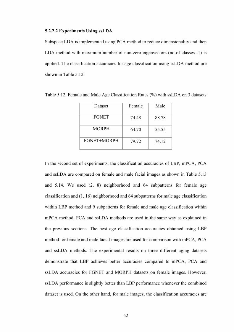
52

5.2.2.2 Experiments Using ssLDA

Subspace LDA is implemented using PCA method to reduce dimensionality and then

LDA method with maximum number of non-zero eigenvectors (no of classes -1) is

applied. The classification accuracies for age classification using ssLDA method are

shown in Table 5.12.

Table 5.12: Female and Male Age Classification Rates (%) with ssLDA on 3 datasets

Dataset Female Male

FGNET 74.48 88.78

MORPH 64.70 55.55

FGNET+MORPH 79.72 74.12

In the second set of experiments, the classification accuracies of LBP, mPCA, PCA

and ssLDA are compared on female and male facial images as shown in Table 5.13

and 5.14. We used (2, 8) neighborhood and 64 subpatterns for female age

classification and (1, 16) neighborhood and 64 subpatterns for male age classification

within LBP method and 9 subpatterns for female and male age classification within

mPCA method. PCA and ssLDA methods are used in the same way as explained in

the previous sections. The best age classification accuracies obtained using LBP

method for female and male facial images are used for comparison with mPCA, PCA

and ssLDA methods. The experimental results on three different aging datasets

demonstrate that LBP achieves better accuracies compared to mPCA, PCA and

ssLDA accuracies for FGNET and MORPH datasets on female images. However,

ssLDA performance is slightly better than LBP performance whenever the combined

dataset is used. On the other hand, for male images, the classification accuracies are

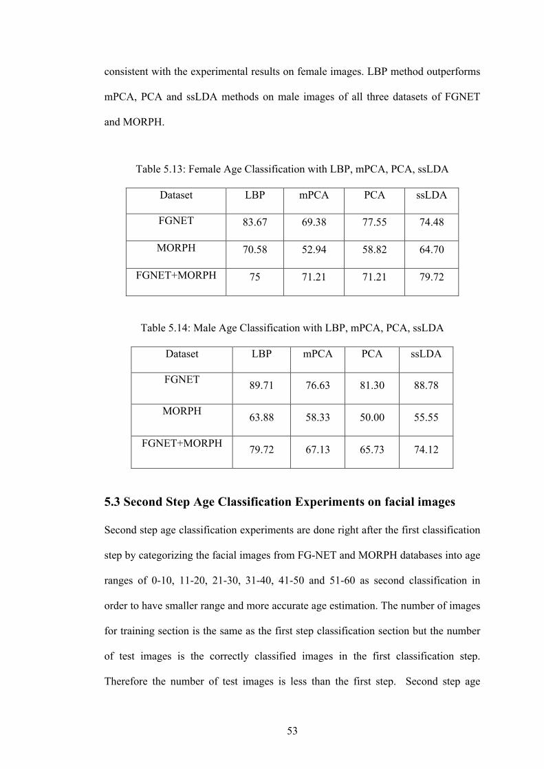
53

consistent with the experimental results on female images. LBP method outperforms

mPCA, PCA and ssLDA methods on male images of all three datasets of FGNET

and MORPH.

Table 5.13: Female Age Classification with LBP, mPCA, PCA, ssLDA

Dataset LBP mPCA PCA ssLDA

FGNET 83.67 69.38 77.55 74.48

MORPH 70.58 52.94 58.82 64.70

FGNET+MORPH 75 71.21 71.21 79.72

Table 5.14: Male Age Classification with LBP, mPCA, PCA, ssLDA

Dataset LBP mPCA PCA ssLDA

FGNET 89.71 76.63 81.30 88.78

MORPH 63.88 58.33 50.00 55.55

FGNET+MORPH 79.72 67.13 65.73 74.12

5.3 Second Step Age Classification Experiments on facial images

Second step age classification experiments are done right after the first classification

step by categorizing the facial images from FG-NET and MORPH databases into age

ranges of 0-10, 11-20, 21-30, 31-40, 41-50 and 51-60 as second classification in

order to have smaller range and more accurate age estimation. The number of images

for training section is the same as the first step classification section but the number

of test images is the correctly classified images in the first classification step.

Therefore the number of test images is less than the first step. Second step age

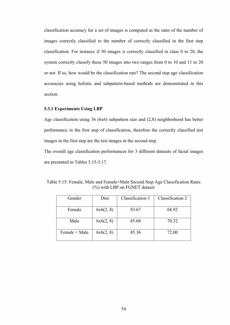
54

classification accuracy for a set of images is computed as the ratio of the number of

images correctly classified to the number of correctly classified in the first step

classification. For instance if 50 images is correctly classified in class 0 to 20, the

system correctly classify these 50 images into two ranges from 0 to 10 and 11 to 20

or not. If so, how would be the classification rate? The second step age classification

accuracies using holistic and subpattern-based methods are demonstrated in this

section.

5.3.1 Experiments Using LBP

Age classification using 36 (6x6) subpattern size and (2,8) neighborhood has better

performance in the first step of classification, therefore the correctly classified test

images in the first step are the test images in the second step.

The overall age classification performances for 3 different datasets of facial images

are presented in Tables 5.15-5.17.

Table 5.15: Female, Male and Female+Male Second Step Age Classification Rates (%) with LBP on FGNET dataset

Gender Dim Classification 1 Classification 2

Female 6x6(2, 8) 83.67 68.92

Male 6x6(2, 8) 85.04 70.32

Female + Male 6x6(2, 8) 85.36 72.00

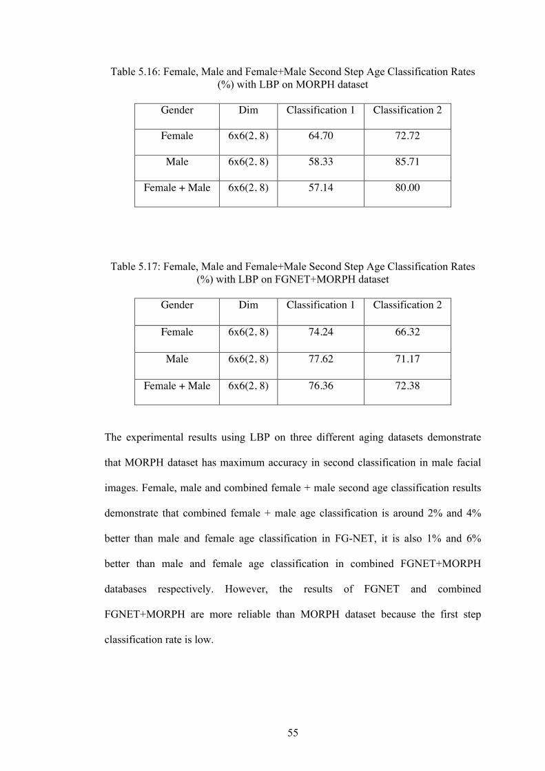
55

Table 5.16: Female, Male and Female+Male Second Step Age Classification Rates (%) with LBP on MORPH dataset


Female 6x6(2, 8) 64.70 72.72

Male 6x6(2, 8) 58.33 85.71

Female + Male 6x6(2, 8) 57.14 80.00

Table 5.17: Female, Male and Female+Male Second Step Age Classification Rates (%) with LBP on FGNET+MORPH dataset


Female 6x6(2, 8) 74.24 66.32

Male 6x6(2, 8) 77.62 71.17

Female + Male 6x6(2, 8) 76.36 72.38

The experimental results using LBP on three different aging datasets demonstrate

that MORPH dataset has maximum accuracy in second classification in male facial

images. Female, male and combined female + male second age classification results

demonstrate that combined female + male age classification is around 2% and 4%

better than male and female age classification in FG-NET, it is also 1% and 6%

better than male and female age classification in combined FGNET+MORPH

databases respectively. However, the results of FGNET and combined

FGNET+MORPH are more reliable than MORPH dataset because the first step

classification rate is low.

56

5.3.2 Experiments Using mPCA

These experiments are done with different subpattern sizes using mPCA. The facial

images from all subsets of the aging databases are divided into 4, 9, 25, 36, 49, 64

and 81 subpatterns. The test images are the correctly classified images in first step

classification. Modular PCA age classification using maximum number of non-zero

eigenvectors is performed for female and male facial images. The overall age

classification performances for 3 different datasets of facial images are presented in

Tables 5.18-5.20. The following notations are used in the tables:

1: represents the first step classification performance,

2: represents the second step classification performance

Table 5.18: Female and Male Second Step Age Classification Rates (%) with mPCA on FGNET dataset

Subpattern

size

Female Male

1 2 1 2

2x2 67.34 51.02 75.70 60.74

3x3 69.38 53.06 76.63 58.87

5x5 66.32 52.04 74.76 54.20

6x6 66.32 51.02 73.83 54.20

7x7 59.18 50.00 72.89 55.14

8x8 62.24 47.95 75.70 57.94

9x9 61.22 46.93 72.89 55.14

57

Table 5.19: Female and Male Second Step Age Classification Rates (%) with mPCA on MORPH dataset

Subpattern

size

Female Male

1 2 1 2

2x2 47.05 38.23 61.11 52.77

3x3 52.94 35.29 58.33 50.00

5x5 55.88 41.17 58.33 47.22

6x6 55.88 44.11 61.11 47.22

7x7 58.82 38.23 58.33 47.22

8x8 50.00 35.29 58.33 47.22

9x9 58.82 41.17 58.33 47.22

Table 5.20: Female and Male Second Step Age Classification Rates (%) with mPCA on FGNET+MORPH dataset

Subpattern

size

Female Male

1 2 1 2

2x2 73.48 53.78 65.73 50.34

3x3 71.21 50.75 67.13 49.65

5x5 68.18 50.00 67.13 47.55

6x6 66.66 49.24 66.43 46.85

7x7 62.87 48.48 65.73 46.85

8x8 67.42 50.00 65.03 48.25

9x9 63.63 48.48 65.73 44.75

58

Modular PCA second age classification results with different subpattern sizes are

different for three datasets. In addition, the results with 4 (2x2) and 9 (3x3)

subpatterns sizes demonstrate better performance in both female and male second

step classification. However, In MORPH dataset the best results is obtained using 36

(6x6) subpatterns size. In addition, male second age classification using 9 subpatterns

is around 5% better than female second age classification in FGNET. However

female second age classification is around 4% better than male second age

classification in combined FGNET+MORPH database.

5.3.3 Experiments Using PCA

The results of classifying ages using Principal Component Analysis technique are

shown in Tables 5.21 to 5.23.

Table 5.21: Female, Male and Female+Male Second Step Age Classification Rates (%) with PCA on FGNET dataset

Gender Classification 1 Classification 2

Female 77.55 61.84

Male 81.30 72.41

Female + Male 81.46 64.67

Table 5.22: Female, Male and Female+Male Second Step Age Classification Rates (%) with PCA on MORPH dataset


Female 58.82 70.00

Male 50.00 94.44


59

Table 5.23: Female, Male and Female+Male Second Step Age Classification Rates (%) with PCA on FGNET+MORPH dataset


Female 71.21 58.51

Male 65.73 73.40


5.3.4 Experiments Using ssLDA

Subspace LDA is implemented using maximum number of non-zero eigenvectors

(no of classes -1). The second classification accuracies for age classification using

ssLDA method are shown in Table 5.24. The following notations are used in the

tables:

1: represents the first step classification performance,

2: represents the second step classification performance.

Table 5.24: Female and Male Second Step Age Classification Rates (%) with ssLDA on FGNET MORPH and FGNET+MORPH dataset

Gender FGNET MORPH FGNET +MORPH

1 2 1 2 1 2

Female 74.48 63.01 79.72 48.83 64.70 40.90

Male 88.78 60.00 74.12 56.60 55.55 65

For the comparison of PCA and ssLDA as holistic approaches it can be concluded

that the result of the second classification rate with PCA and ssLDA on FGNET

dataset is better than MORPH and combined FGNET+ MORPH. The best result is

60

obtained with FGNET on male facial images due to the maximum rate in the fist and

second step classification which is 81% and 72% respectively.

In general, the experiments on the second step classification demonstrate that LBP

and PCA approaches achieve the better results on FGNET dataset in male facial

images. It is clearly shown that second classification achieves the best classification

rates when the rate of first step classification is high.

5.4 Ratio Analysis

Ratio analysis is applied on facial images in which primary features are located and

labeled in order to separate babies from adults.

5.4.1 Age classification Experiments using two ratios

Ratio analysis is applied on 528 images of FGNET dataset, which includes 39 babies

from 0 to 2 years old. Table 5.25 demonstrates the baby classification rate in FGNET

dataset with different conditions.

Ratio1 values are obtained using

𝑅!" = !!"!!!

and Ratio2 values are obtained using

𝑅!"# = !!"!!"

61

Table 5.25: Baby Recognition Rates (%) with two Ratio analysis on FGNET dataset

Condition Rate Condition Rate

Ratio1< 0.80 53.84 Average of Ratios < 1.52 53.84

Ratio1< 0.81 71.79 Average of Ratios < 1.56 87.17

Ratio1 < 0.82 100 Average of Ratios < 1.58 100

Ratio 2 < 1.31 69.23 Ratio1< 0.86 and ratio2 < 1.50 71.79


Ratio 2 < 1.35 79.48 Ratio1< 0.86 and ratio2 < 1.65 100



The values of Ratio1 and Ratio2 are closed to each other therefore the small change

in the condition can change the accuracy of recognizing the babies. Using the ratio

values can be reliable when all the images are frontal and the primary features are

located carefully on the same line of coordinates. Using the ratio analysis cannot be

an appropriate system alone because the differentiation is difficult.

Some values of Ratio 1 and Ratio 2 are shown in Table 5.26 and Table 5.27.

62

Table 5.26: Ratio1 and Ratio2 values of some FGNET images

Name Age Ratio1 Ratio2 AVG Name Age Ratio1 Ratio2 AVG

019a00 0 0.78 1.21 1.00 072a27 27 0.90 2.26 1.58

023a00 0 0.83 1.28 1.05 001a28 28 1.03 2.20 1.61

015a01 1 0.81 1.78 1.30 061a29 29 0.90 1.90 1.40

073a01 1 0.89 1.95 1.42 072a29 29 0.95 2.25 1.60

011a02 2 0.84 1.30 1.07 005a30 30 1.04 1.98 1.51

026a02 2 0.90 2.30 1.60 029a31 31 0.98 1.52 1.25

002a03 3 0.87 1.35 1.11 061a32 32 0.89 1.54 1.22

046a04 4 0.89 1.94 1.42 067a33 33 0.87 2.11 1.49

011a05 5 0.89 1.57 1.23 012a34 34 0.99 2.09 1.54

008a06 6 0.78 1.72 1.25 062a35 35 0.95 1.39 1.17

081a07 7 0.89 1.79 1.34 006a36 36 0.98 1.36 1.17

001a08 8 0.91 2.24 1.57 028a37 37 0.94 1.52 1.23

060a08 8 0.88 1.69 1.28 002a38 38 0.95 1.41 1.18

035a09 9 1.01 1.56 1.29 021a39 39 1.11 1.83 1.47

037a09 9 0.84 1.37 1.11 011a40 40 0.94 1.59 1.27

056a10 10 0.94 1.63 1.29 072a41 41 0.97 2.73 1.85

081a10 10 0.89 2.37 1.63 017a42 42 1.00 1.89 1.44

075a11 11 0.90 1.97 1.43 045a43 43 1.04 1.74 1.39

63

Table 5.26 (continued)

Name Age Ratio1 Ratio2 AVG Name Age Ratio1 Ratio2 AVG

031a12 12 1.01 1.98 1.49 071a44 44 0.91 1.48 1.19

036a13 13 0.94 1.93 1.44 007a45 45 0.96 1.62 1.29

050a14 14 0.98 1.89 1.43 048a46 46 0.97 1.67 1.32

056a15 15 0.85 2.11 1.48 004a48 48 0.92 2.56 1.74

082a16 16 1.03 1.97 1.50 048a49 49 0.92 1.71 1.31

076a17 17 0.88 2.09 1.48 048a50 50 0.92 1.62 1.27

001a18 18 0.95 2.73 1.84 004a51 51 0.97 2.13 1.55

005a18 18 1.01 2.08 1.54 039a52 52 0.97 1.71 1.34

061a19 19 0.92 1.64 1.28 048a54 54 1.00 1.84 1.42

002a20 20 0.99 2.26 1.62 047a55 55 0.93 1.73 1.33

082a21 21 0.94 1.52 1.23 003a58 58 1.04 1.89 1.47

007a22 22 0.99 1.50 1.25 003a60 60 1.01 2.13 1.57

057a23 23 1.00 1.97 1.48 005a61 61 0.94 1.79 1.36

071a23 23 0.94 1.66 1.30 006a61 61 1.01 1.29 1.15

005a24 24 1.07 2.16 1.62 004a62 62 1.00 1.74 1.37

061a25 25 0.88 1.64 1.26 004a63 63 0.95 3.29 2.12

002a26 26 0.99 1.74 1.36 006a67 67 1.00 1.38 1.19

048a27 27 0.98 1.66 1.32 006a69 69 1.04 1.29 1.16

64

Table 5.27: Ratio values of MORPH images

Name Age Ratio 1 Ratio 2 AVG

24928_1M28 28 0.82 1.40 1.11

30238_1M29 29 0.83 1.25 1.04

29201_0M30 30 0.94 1.26 1.10

42603_2M31 31 0.94 1.30 1.12

24928_2M32 32 0.92 1.43 1.17

42585_1M33 33 1.01 1.24 1.13

29201_1M36 36 0.98 1.08 1.03

30238_2M37 37 0.85 1.61 1.23

28926_2M38 38 0.98 1.33 1.15

30148_0M39 39 0.95 1.24 1.09

27534_3M42 42 0.91 1.53 1.22

28234_2M43 43 0.85 1.18 1.01

32752_1M45 45 1.06 0.66 0.86

24940_1M46 46 1.21 1.53 1.37

26845_1M47 47 0.89 1.26 1.07

32620_1M48 48 0.89 2.16 1.53

33027_1M50 50 0.95 1.18 1.06

32659_0M53 53 0.98 1.53 1.25

22008_2M55 55 1.15 1.19 1.17

9974_1M58 58 0.93 1.61 1.27

32659_1M61 61 0.92 1.76 1.34

27880_2M68 68 1.45 1.44 1.44

65

The values of Ratio1 and Ratio2 show that the value of Ratio1 and Ratio2 in babies

is less than the values of Ratio1 in adults. It is not always true because all of the

images are not frontal and the primary features are not in the same line of

coordinates. Therefore, using ratio analysis algorithm may be not a reliable algorithm

in all cases discussed above and it highly depends on facial images’ poses.

66

Chapter 6

CONCLUSION

In this thesis, we have presented a performance analysis of subpattern-based LBP

and subpattern-based mPCA approaches with holistic PCA and holistic ssLDA

approaches for the solution of age classification problem. The experiments

performed using three different datasets obtained from FG-NET and MORPH aging

databases demonstrate the efficiency of LBP method over the other methods on both

female and male facial images in first and second step classification. In the case of

female age classification, LBP achieves better accuracies compared to mPCA, PCA

and ssLDA performance on FG-NET and MORPH datasets. Age classification on

male images demonstrates the superiority of LBP method on all datasets of FG-NET

and MORPH. In general, it can be stated that LBP achieves better results for age

classification on both female and male facial images for different datasets of FGNET

and MORPH databases.

Future work on age classification can be focused on the following investigations:

• From a practical point of view, age classification methods should focus on the

contributions of shape-based features and texture-based features in age

classification from facial images.

• As a texture-based features algorithm, Weighted Local Binary Patterns

(WLBP) can be used to investigate which regions are more important in

aging process.

67

• Moreover, Support Vector Machines (SVM) in most of the classification

algorithms have achieved the best accuracy in linear and nonlinear

classification, therefore SVM can be applied for age classification to examine

the accuracy rate in smaller age intervals.

68

REFERENCES

[1] A. Lanitis, C. Draganova, and C. Christodoulou. Comparing different classifiers

for automatic age estimation. IEEE Transactions on Systems, Man, and

Cybernetics, 34(1):621–628, 2004.

[2] Y. H. Kwon and N. da Vitoria Lobo, ‘Age Classification from Facial Images’,

Computer Vision and Image Understanding Journal 74(1), pp. 1–21, 1999.

[3] http://www.scholarpedia.org/article/Facial_Age_Estimation

[4] Xin Geng, Zhi-Hua Zhou, and Kate Smith-Miles. Automatic age estimation

based on facial aging patterns. IEEE Transactions on Pattern Analysis and

Machine Intelligence, 29(12):2234–2240, 2007.

[5] Z. Yang and H. Ai. Demographic classification with local binary patterns. In

Proc. of International Conference on Biometrics, pages 464–473, 2007.

[6] Y. Fu and T.S. Huang, ‘Human Age Estimation with Regression on

Discriminative Aging Manifold’, IEEE Transactions on Multimedia, 10(4), pp

578-584, 2008

[7] M. G. Rhodes, ‘Age Estimation of Faces: A Review’(2009), Appl. Cognitive

Psychology. 23, pp 1–12.

69

[8] Ramanathan, N., Chellappa, R., Biswas, S. , “Age progression in Human Faces:

A Survey”, Accepted for publication in Journal of Visual Languages and

Computing (Special Issue on Advances in Multimodal Biometric Systems), 2009.

[9] L. S. Mark, J. T. Todd, and R. E. Shaw, “Perception of growth : A geometric

analysis of how different styles of change are distinguished,” Journal of

Experimental Psychology : Human Perception and Performance, vol. 7, pp. 855–

868, 1981.

[10] N. Ramanathan, R. Chellappa, S. Biswas, Computational Methods for Modeling

Facial Aging: A Survey, Journal of Visual Languages and Computing, 2009.

[11] J. Huang, B. Heisele and V. Blanz, Component-based Face Recognition with 3D

Morphable Models, AVBPA, 2003.

[12] P. Pujol, D. Macho, C. Nadeu, “On Real-Time Mean-and-Variance

Normalization of Speech Recognition Features”. IEEE International Conference

on Acoustics, Speech and Signal Processing, 2006. ICASSP 2006 Proceedings.

Volume 1, I–I, 14-19 May 2006.

[13] Z. Gengtao, Z. Yongzhao, Z. Jianming, “Facial Expression Recognition Based

on Selective Feature Extraction”. Sixth International Conference on Intelligent

Systems Design and Applications, 2006. ISDA '06. Volume 2, 412-417, Oct.

2006.

70

[14] T. Ojala, M. Pietikaïnen, and D. Harwood, “A Comparative Study of Texture

Measures with Classification Based on Feature Distributions,” Pattern

Recognition, vol. 29, no. 1, pp. 51-59, 1996.

[15] T.Ahonen, M.Pietikainen, “Face Description with Local Binary Patterns:

Application to Face Recognition,” IEEE Trans. Pattern Analysis and Machine

Intelligence, vol. 28, no. 12, December 2006.

[16] T. Ojala, M. Pietikainen, and T. Maënpaä¨, “Multiresolution Gray-Scale and

Rotation Invariant Texture Classification with Local Binary Patterns,” IEEE

Trans. Pattern Analysis and Machine Intelligence, vol. 24, no. 7, pp. 971-987,

July 2002.

[17] P.N. Belhumeur, J.P. Hespanha, D.J. Kriegman, Eigenfaces vs. Fisherfaces:

Recognition Using Class Specific Linear Projection, IEEE Trans. Pattern

Analysis and Machine Intelligence, 19(7), 1997, 711-720.

[18] X. Wang, and X. Tang, Random Sampling for Subspace Face Recognition,

Interntional Journal of Computer Vision, 70(1), 2006, 91-104.

[19] Vytautas Perlibakas, “Distance measures for PCA-based face recognition”.

Pattern Recognition Letters, Volume 25, Issue 6, 711-724, 19 April 2004.

[20] R. Gottumukkal and V.K. Asari, An improved face recognition technique based

on modular PCA approach, Pattern Recogn. Lett. 25 (2004) (4), pp. 429–436

71

[21] S. Chen, Y. Zhu, Rapid and Brief Communication Subpattern-based principal

component analysis. 3 September 2003, Pattern Recognition Society, Volume 37,

Issue 5, May 2004, Pages 1081-1083

[22] J. Huang, B. Heisele and V. Blanz, Component-based Face Recognition with 3D

Morphable Models, AVBPA, 2003.

[23] M. Turk and A. Pentland, Eigenfaces for Recognition, Journal of Cognitive

Neuroscience, 3(1), 1991, 71-96.

[24] P.N. Belhumeur, J.P. Hespanha, D.J. Kriegman, “Eigenfaces vs. Fisherfaces:

Recognition Using Class Specific Linear Projection”, IEEE Trans. Pattern

Analysis and Machine Intelligence, 19(7), 1997, 711-720.

[25] F. Song, H. Liu, D. Zhang, J. Yang, A Highly Scalable Incremental Facial

Feature Extraction Method, Neurocomputing, 71, 2008, 1883-1888.

[26] L. S. Mark, J. B. Pittenger, H. Hines, C. Carello, R. E. Shaw, and J. T. Todd,

“Wrinkling and head shape as coordinated sources of age level information,”

Journal of Perception and Psychophysics, vol. 27(2), pp. 117–124, 1980.

[27] W. B. Horng, C. P. Lee and C. W. Chen ”Classification of Age Groups Based

on Facial Features”, Tamkang Journal of Science and Engineering, Vol. 4, No. 3,

pp. 183-192, 2001.

[28] http://www.isbe.man.ac.uk/~bim/software/am_tools_doc/index.html

72

[29] The FG-NET Aging Database:

http://sting.cycollege.ac.cy/~alanitis/fgnetaging/index.htm

[30] Ricanek, K., Tesafaye, T., “MORPH: A Longitudinal Image Database of

Normal Adult Age-Progression “, 7th International Conference on Automatic

Face and Gesture Recognition, Southampton, UK, pp 341-345 (2006).

[31] G. Guo, Y. Fu, C. R. Dyer, and T.S. Huang, ‘Image-Based Human Age

Estimation by Manifold Learning and Locally Adjusted Robust Regression’,

IEEE Transactions On Image Processing, 17(7), pp 1178-1188, 2008.

[32] Lanitis, A., “A survey of the effects of aging on biometric identity verification,

”International Journal of Biometrics (IJBM), Vol. 2, No. 1, pp. 34 – 52 (xxxx).

[33] TorchVision C++ Program, http://www.torch3vision.idiap.ch

Age Classification using Facial Feature Extraction

Documents

Transcript of Age Classification using Facial Feature Extraction