AD-758 589

AGARD FLIGHT TEST INSTRUMENTATION SERIESVOLUME 2. IN-FLIGHT TEMPERATURE MEASURE-MENTS,

F. Trenkle, et al

Advisory Group for Aerospace Research andDevelopmentParis, France

February 1973

g, I

DISTRIBUTED BY:5 TUMNatonl Technical Infmation ServiceU. S. DEPARTMENT OF COMMERCE5285 Port Royal Road, Springfield Va. 22151

j

AGARD..AG-160VOL. 2

-DD

AGARDograph No. 160

AGARD Flight Test Instrumentation Series

Volume 2on

In-Flight Temperature Measurementsby

F.Trenkle and M.Reinharddt

DISTRIBUTION AND AVAILABILITYON BACK COVER

-AI

AGARD-AG-160Volume 2

NORTH ATLANTIC TREATY ORGANIZATION

ADVISORY GROUP FOR AEROSPACE RESEARCH AN!D DEVELOPMENT

(ORGANISATION DU TRAITE DE L'ATLANTIQUE NORD)

AGARDograpb No. 160 Vol.2

IN-FLIGHT TEMPERATURE MEASUREMENTS

by

F.Trenkle and M.Reinhardt

Volume 2

of the

AGARD FLIGHT TEST INSTRUMENTATION SERIES

Edited by

W.D.Mace and A.Pool

This AGARDograph has been sponsored by the Flight Mechanics Panel of AGARD.

r

THE MISSION OF AGARD

The inission of AGARD is to bring together the leading pl rsonalities of tP!! NATO nations in the fields ofscience aiJ technology relating to aerospace for the following purpeses:

- Exchanging of scientific and technical information;

- Cointinuously stimulating advances in the aerospace sciences relevant to strengthening the common defenceposture;

b-- lproving- the co-operation among member nations in aexospace research and development;

- Providing scientific and technical advice and assistance to the North Atlantic Military Committee in thefield of aerospace research and development;

- Rendering scientific and technical assistance, as requested, to other NATO bodies and to member nations

in oonnection with research and development problems in the aerospace field;

- Providing assistance to member nations for the purpose of increasing their scientific and technical potential;

"- Recommending effective ways for the member nations to use their research and development capabilitiesfor the common benefit of the NATO community.

The highest authority within AGARD is the National Delegates Board consisting of officially appointed seniorrepresentatives from each member nation. The mission of AGARD is carried out through the Panels which are

.4 composed of experts appointed by the National Delegates, the Consultant and Exchange Program and the Aerospace

Applications Studies Program. The results of AGARD work are reported to the member nations and the NATOAuthorities through the AGARD series of publications of which this is one.

Participation in AGARD activities is by invitation only and is normally limited to citizens of the NATO nations.

The material in this publication has been reproduceddirectly from copy supplied by AGARD or the author.

Published February 1973

629.73:536.5

Printed by Technical Editing and Reproduction LtdHarford House, 7-9 Charlotte St. London. WIP IHD

PREFACE

Soon after its foundation in 1952, tihe Advisory Group for Aeronautical Researchand Development recognized the need for a comprehensive publication on1 flight testtechniques and the associated instrumentation. Under tihe direction of tihe AGARDFlight Test Panel (now the Flight Mechanics Panel), a Flight Test Manual waspublished in the years 1954 to 1956. The Manual was divided into four volumes:1. Performance, II. Stability and Control, Ill. Instrumentation Catalog, and IV.Instrumentation Systems.

Since then flight test in.strumentation has developed rapidly in a broad field ofsophisticated techniques. In view of thifs developmnent the Flight Test InstrumentationCommittee of the Flight Mechanics Panel was asked in 1968 to update Volumes IIIand IV of the Flight Test Manual. Upon the advice of the Committee, the Panel..decided that Volume I1l would not be continued and that Volume IV would bereplaced by a series of separately published nionogiaphs on selected subjects offlight test tnstninentation: the AGARD) Flight Test Instrumentation Series. The firstvolume of this Series gives a general introduction to the basic principles of flight testinstrumentation engineering' and is composed from contributions by several specialized

e authors. Each of the other volumes p~rovides a more detailed treatise by a specialist on•, a selected instrumentation subject. Mr W.D.Mace and Mr A.Pool were willing to acceptS~the responsibility of editing the Series, and Prol: D.Bosman assisted them in editing the; introductory volume, AGARD) was fortunate in finding competent editors and authorsS~willing to contribute their knowledge and to spend considerable time in the preparation• . of this Series.

It is hoped that this Series will satisfy the existing need for specialized documnen-

• tation in the field of flight test instrumecntation and as such may promote a better

',understanding between the flight test engineer and the instrumentation and data• processing specialists. Such understanding is essential for the efficient design and

i •' execution of flight test programs.

~assistance of the Flight Mechanics Panel in the preparation of this Series are greatly

£1 appreciated." ~ T.VAN OOSTEROM

CONTENTS

Page

PREFACE . . . . . . . . . . . . . . . . . . . . .

LIST OF SYMBOLS .. .. ............ .............. .............. .............. .............Vill

1. INTRODUCTION............................. .. .......... . . ... . . ..... .. .. .. .. .. .... 1

1.1 Aim of this Volume...................... . .. ..... . . ... . . .... .. .. .. .. .. .... 1

1.2 Temperature Heasuremepts in Aircraft .. .. ............ ............ ..................2

1.3 Thermometers Used in Aircraft. .. ............ .............. .............. ......... 2

2. RESISTANCETEMPERATURE MEASUREMENTS .. .. .......... ................ ............ ......... 4

2.1 Resistance Probes. .. .............. ............ .............. .............. ..... 4

2.1.1 Elements with Positive Temperature Coefficients. .. ...... .............. ....... 5

2.1.2 Resistance Materials with Negligible Temperature Coefficient......... ......... 6

2.1.3 Elements with Negative Temperature Coefficients. .. ...... .............. ....... 7

2.1.4 Construction of Resistance Elements. .. ...... .............. .................. 8

2.1.5 Construction of Resistance Probes......... ..... . . .. . . .... .. .. .. .. .. .... 8

2.2 Circuits and Indicators for Resistance Thermometere. .. .............. ................ 10

2.2.1 Bridge Circuits .. .. ............ .............. .............. ..............10

2.2.2 Compensation of Lead Resistances. .. .............. .............. ............11

2.2.3 Design of Bridge Circuits..... .. .. .. .. .. .. .. .. .. .. .. .. .. 12

2.2.3.1 Half Bridge Circuits .. .. ............ .............. ................13

2.2.3.2 Full Bridge Circuits .. .. ............ .............. ................15

2.2.4 Direct Indicators .. .. ............ .............. .............. ............17

2.2.5 Servoed Indicators. .. .............. .............. ............ ............17

2.2.5.1 Servoed, AC Bridges. .. ...... .............. .............. .......... 18

2.2,,5.2 Servoed DC Bridges. .. ...... .............. .............. .......... 18

2.2.6 Bridges with Special Output for Recording. .. ...... .............. ............19I

3. THERMOELECTRIC TEMPERATURE MEASURmEMENTS. .. ...... .............. .............. ..........21

3.1 Thermocouple Probes. .. .............. ................. ..... .. .. .. .. .. ........ 213.1.1 Thermocouples .. .. .... ....... . ...... ....... . ...... ....... ..... .......... .. 213.1.2 Construction of Thermocouples.. ...... .. ...... .............. ................21

3.1.3 Construction of Probes with Thermocouples. .. ...... .............. ............ 23

3.2 Connecting Wires and Extension Leads .. .. ............ .............. ................ 24

3.3 Indicators for Thermocouples. .. ...... .............. .............. ................ 26

3.3.1 Direct Indicators .. .. ............ .............. .............. ............26

3.3.2 Servoed Indicators. .. .............. ............ .............. ............ 26

4. HEAT TRANSFER AND TEMPERATURE RECOVERY .. ...... .............. .............. ............27

4.1 Modes of Heat Transfer .. .. ............ .............. ............ ................27

4.2 Heat Transfer between Iuaobile Materials .. .. ............ .............. ............ 28

4.2.1 Heat Transfer between Solids. .. .............. ............ .................. 28

4.2.2 Heat Transfer between a Solid cmd an Insmobile Gas or Liquid .. .. ................ 30

4.3 !Seat Transfer between a Solid and a Flowing Gas or Liquid .. .......... ................ 30

4.3.1 Velocity and Temperature boundary-Layers. .... ............ .............. ..... 30

4.3.2 Heat Transfer by Natural Convection. .. ........ .............. ................ 31

4.3.3 Heat Transfer by Forced Convection .. ........ .............. ..................31

4.3.3.1 Heat Transfer i.n a Subsonic Flow .. .. ............ .............. ..... 31

4.3.3.2 Temperatures of a High-Velocity Flow. .. ........ .............. ....... 32

4.3.3.3 Temperature Measurement in a Supersonic Flow .. .. .............. ....... 35

5. REFERENCE VALUES, ERRORS AND DEFINITIONS OF TEMPERATUR.E MESUPJ2(ENT .. .. .............. ..... 36

5.1 Reference Values of Temperature Measurement. .... .............. .............. ....... 36

5.1.1 Static Temperature .. ........ ................ .............. ................ 36

5.1.2 Temperature Definitions Related to Static Temperature .. .. .............. ....... 37

5.1.3 Total Temperature. .. ........ .............. .............. ..................38

5.1.4 Temperature Definitions Related to Total Temperature. .. ................ ....... 39

5.2 Errors of Temperature Measurements .. .. .............. .............. ................41

5.2.1 Meteorological Errors . . . ......... ................................................. 43

5.2.2 Position Errors. .. ...................... .............. .............. ..... 45

5.2.3 Temperature Lag Error 4....... .... .. .. .. .. .. .. .. .. ..... 53

5.2.4 Instrument Error E . . . . .. .. . .. .. .. . .. .... ... .. . .. .. .. .. . .. .. .. . .. .. ... .. 56

6. PRACTICAL TEMERATURE MEASUREMENTS. .... ................ .. ............ ............ ..... 59

6.1 Different Types of Temperature Measurenenta. .... ............ .............. ......... 59

6.1.1 Measurementsin outside Air .. .. ................ ............ ................ 59

6.1.2 Temperature Measurements in Air and Ganes of Engines. .... .............. ....... 62

6.1.2.1 Important Engine Temperatures. .... .............. .............. ..... 62

6.1.2.2 Selection of Temperature Probes . . . . . . ................................... 63

6.1.2.3 Selection of Probe Locations .. .. ................ ............ ....... 64

6.1.3 Temperature Measuroments in Liquids. .. ........ .............. ...............64

6.1.4 Temperature Measurements on Surfaces and Solids. .. ........ ...................65

Selection of Thermo~meters.. .......... .............. .............. .............. 67

Calibration of Thermometers. .... .............. .............. .......... ....... 69

6.3.1 Calibrations in the Laboratory .. ........ .............. .............. ....... 69

6.3.2 Flight Line Calibrations. .... .............. ............ .................71

6.3.3.1 General .. .......... ............ .............. .............. ..... 72

6.3.3.2 Explanatory Examples. .. ........ .............. .............. ....... 74

6.3.3.3 Practical Implementation. .. ........ ................................77

6.4 Data Evaluation. .. .............. .............. .............. .............. ......o

6.4.1 Error Handling .. .......... ............ ................ ............ ....... 80

k ~6.4.2 Data Evaluation and Error Correction .. ........ .............. ................84

CONCLUSION. .. .............. .............. .............. .............. ..................88

ACKNOWLEDGEMENTS .. ........ .............. .............. .............. .............. ..... 91

Vi

V REFEDICIS . . . . .. . . . .*. . *. . . . * . . . . . . 97

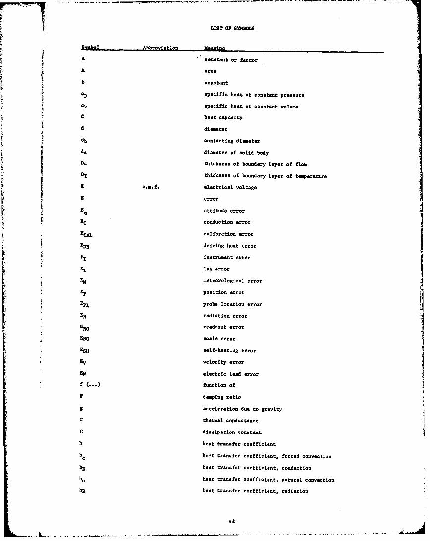
LIST OF ST5LS6

Symbol Abbreviat).on Meanini

a a constant or factor

A area

b constant

c, specific heat at constant pressure

CV cspecific heat at constant volume

C heat capacity

d diameter

Sdb contacting diameter

Ld diameter of solid body

Da thickness of boundary layer of flow

DT thickness of boundary layer of temperature

E e.u.f. electrical voltage

E error

Ea attitude error

EC conduction error

ECAL calibration error

EDH deicing heat error

SE instrument error

EL lag error

EM meteorological error

Ep position error

EpL probe location error

ER radiation error

ERO read-out error

ESC scale error

ESH self-heating error

EV velocity error

EW electric lead error

f (...) function of

F damping ratio

g acceleration due to gravity

G thermal conductance

G dissipation 4onstant

h heat transfer coefficient

h hent transfer coefficient, forced convectionhD heat transfer coefficient, conduction

hn heat transfer coefficient, natural convection

hR heat transfer coefficient, radiation

Viii

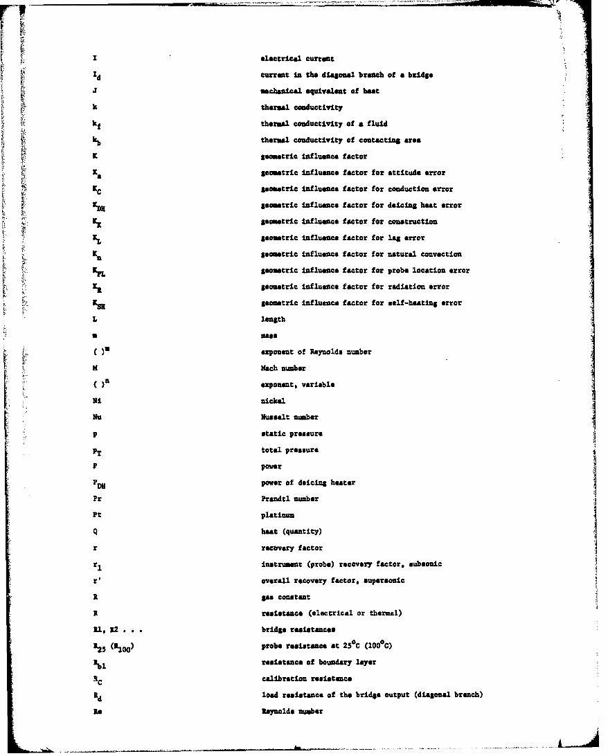
• zelectrica current •" d current In the diagonal branch of a bzidle

J Mechanical equivalent of beat

k theruml conductivity

kf thermal conductivity of fltuid

kb• •thermal conductivity of contacting area

_ geometric influence factor

geometric influence factor for attitude error

VgC geometric Influence factor for conduction error

geometric Influence factor for deicing hbet error

KK geometric influece factor for construction

" •geometric Influence factor for Ua error

g geometric Influence factor for natural convection

geometric influence factor for probe location error

K& geometric Influence factor for radiation error

geometric influence factor for self-heating error7L length

a mass

, ( )m eponent of Reynolds number

l KMach number

-( )n eponent, variable

I Ni nickel

NU Nuseelt number

p static pressure

PT total pressure

P power

PDH pover of deicing heater

Pr Prandtl number

Pt platinum

Q heat (quantity)

r recovery factor

r instrument (probe) recovery factor. lsubsonic

r' overall recovery factor, eupereonic

R as conetaent

R resistance (electrical or thermal)

Rl1 R2 . . . bridge resistances

Rt25 (R300) probe resistance at 250 C (1000C)

R resistance of boundary layer

!1tC calibration resistance

Rd load resistance of the bridge output (diagonal branch)

Re Reynolds number

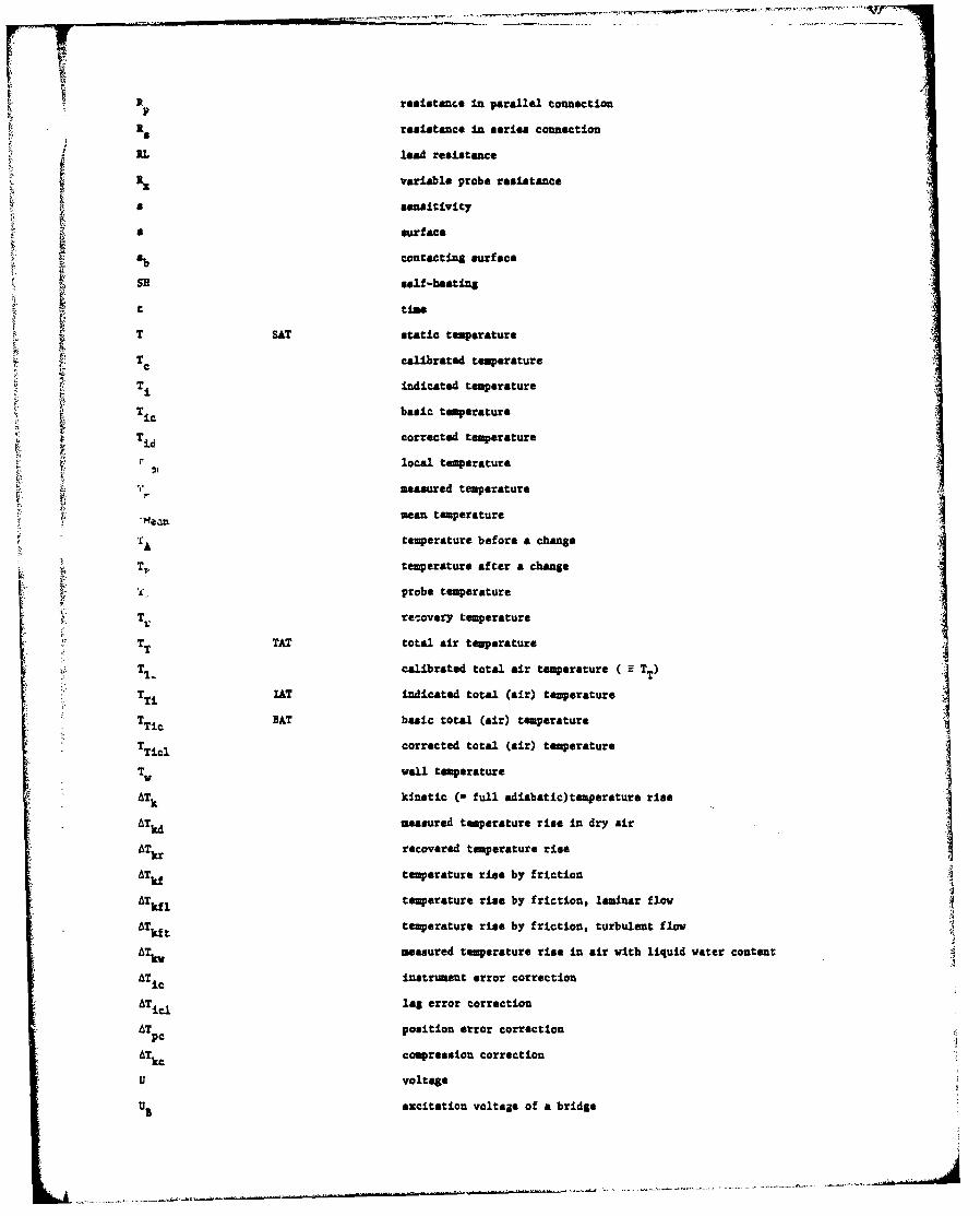
1 .p resistance In parallel connection

* eresistance In series connection

RL lead resistance

fR, variable probe reisatance

s ,enitivity

a surface

F contacting surfaceF: SD$ self-baitin

t time

t T SAT static temperature

'T c calibrated temperature

T indicated temperature

T ic basic temperature

Tid corrected temperature

local temperature

measured temperature

S"Qean mean temperature

LA£ temperature before a change

ST. temperature after a change

probe temperature

STV. re'covery temperature

7T TAT total air temperature

.Tl calibrated total air temperature ( TT)

IAT indicated total (air) temperature

r•T~ BAT basic total (air) temperature

T~ici corrected total (air) temperature

TV wall temperature

ATk kinetic (a full adiabatic)temperature rise

ATM measured temperature rime in dry air

ATkr recovered temperature rise

A~k3 temperature rise by friction

ATk 1 temperature rice by friction, laminar flow

ATk temperature rise by friction, turbulent flow

AT k measured temperature rise in air with liquid water content

ATic inatrument error correction

AT ic lag error correction

AT position error correctionpc

AT compression correctionkcU voltage

U B excitation voltage of a bridge

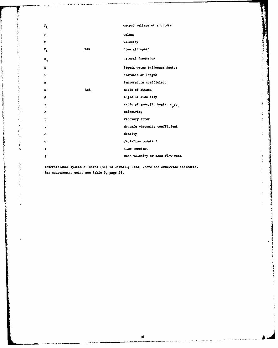
UA output voltage of a bric;e

v volume

V velocity

Vt TAS true air speed

n natural frequency

W liquid water influence factor

x distance or length

1 atemperature coefficient

SAoA augle of attack

SB angle of side slip

Y ratio of specific heats c/Cp v

C emissivity

Sn recovery error

dynamic viscosity coefficient

Sdensity

o radiation constant

time constant

S•mass velocity or mass flow rate

International system of units (SI) is normally used, where not otherwise indicated.

For measurement units see Table 5, page 29.

xi

IN-FLIGHT TEMPPATURE MEASU2(E4iS

by

Fritz Trenkle and Manfred ReinhardtDeutsche Forschungs - und Versuobsanstalt fur Loft - und Raunfahrt E.V.

Institut fuir Physik der AtmosphireOberpfaffenhofen

Germany

SUMARY

Ths publication 13 intended to give practical assistance to all instrumentation and test

engineers working in the field of temperature measurements in aircraft at Mach numbers up to 2.3 and

altitudes up to 80,000 feet.

After a general discussion of the requirements of aircraft temperature measurements, and the

available temperature sensing technology, the detailed techniques of using resistance probes and

thermocouples, as well as the associated electrical leads, circuits, and indicators, are explained. A

discussion of heat transfer processes, primarily between moving fluids and solids, includes terminology,

the systematics of temperature measurements, and the concept of total temperature as the main operational

parameter. An extensive section deals with errors in temperature measurements, as functions of various

parameters, in gases, liquids and solids. Typical laboratory and in-flight calibration techniques for

thermometers are- described, followed by discussions of data handling, error analysis, and the limits of

present methods.

1. DiTRODUCTION

1.1 Aim of this Volume

Temperatures to be measured in and on aircraft presently range Letween approximately 200 and001,500°K, and in extreme cases, the limits extend to 200 K and 2,000°K. Extremely different requirements

are made on the measurement devices depending on the type of measurement (outside air, exhaust, fuel,

etc.). The large number of temperature measurements normally made in a modern production aircraft is

further increased for flight test programs, and there are increased requirements for measurement accuracy,

as well as additional demands, e.g. for matching withrecorders, indicators, and signal conditioners.

The information required to make more precise measurements in aircraft is usually not found in the

regular textbooks on temperature measurement, but have to be gleaned from different individual publications,

and are, therefore, not readily at the disposal of the engineer who suddenly finds himself faced with a

new measurement problem. In the more popular handbooks for flight testing, the measurement of thetemperature of the outside air is briefly discussed. This discussion is, however, often based on the

level of technology in 1945 and the flight regime of the typical piston engine aircraft of tile day.

The possibilities opened up by the development of modern equipment are not often explored. Special

problems are usually ignored, for example, the case of extremely slow-flying aircraft (VTOL) or very fast,

high-altitude aircraft, and the measurement of the temperature of the air as it enters a jet engine.

The following survey should serve the test engineer as well as the instrumentation engineer as

a practical handbook which can be used to choose the correct probes, indicators and signal conditioners,

ascertain their optimum installation, determine their accuracy and correctly interpret the measurements

obtained. Special importance is attached to directly applicable graphic representations in order to

reduce computational work. The examples also show the extent to which data, that are considered

generally valid in normal measurement techniques, can change when measurements are made in air or in

other gases. In the discussion of the processes of heat transfer and the effect of the individual

parameters, the number of problems involved often necessitated an extremely simplified representation,

appropriate for the given measurement purposes, to maintain clarity and because of the limited scope of

this paper. Thus, this paper is intended to be a supplement to the references and manuals which are now

available to the technician. Additional information can be found in the bibliographic list of primary

sources.

For measuring the outside air temperature, the authors have limited themselves to the range of

altitudes and speeds of modern production aircraft. These limits were set at an altitude of 80,000 feet

and a speed af approximately Mach 2.3. The results of measurements made on experimental and test

aircraft which exceeded these limits, insofar as the results have been published, do not enable any

generally valid conclusions to be made. But even in the flight regime selected, there are still zones

for which there are no valid measurement results. This is especially true at relatively low spevds at

high altitudes, in the near~-sonic airspeed range at low altitudes with high atmospheric temperatures

combined with high humidity, and for flights in clouds and heavy rain.

1.2 Temperature Measurements in Aircraft

Figure 1 gives a survey of the different types of temperature measurements in aircraft as well

as the corresponding measurement range.

One of the moat important values is the undisturbed ouzside or static air temperature (SAT).

For reasons of measurement accuracy, the increased total air temperature (TAT),* which depends on the

corresponding Mach number, is almost always determined instead of the static air temperature except on

very slow-flying types of aircraft. If Mach number is determined, TAT is readily converted to static air

temperature. In many aircraft, the ccnversion is done automatically in a central air data computer, which

uses the temperature value and the Mach number to yield the true airspeed (TAS) and other additional

values, e.g. air density, which are necessary for the automatic pilot and the weapons system.

Other important temperature measurements are made in engines to insure that limiting temperatures

are not exceed~ed. For piston engines it is necessary to measure and observe the oil temperature, the

cylinder head temperature, the coolant temperature *and if needed, the carburetor temperature or the air

inlet temperature for injection engines. For jet engines the compressor inlet temperature determines

important operating parameters* so that it must be I~ndicated directly as well as fed to the automatic

fuel control system. Accurate total temperature measurements of the exhaust gas temperature are also

required. There is a logarithmic relation between this temperature and the life of the engina~. The

optimum engine output can, however, only be reached at or near the prescribed temperature, so that the

exhaust temperature must also be measured and indicated continuously. on supersonic aircraft it is alsofed into an automatic nozzle area control system.

Additionally, the measurement and indication of the fuel temperature is often necessary if, for

example, aerodynamic heating of the aircraft skin influences the fuel temperature.

For flight test purposes, w'st of the previously mentioned measurements Must be made with

*increased accuracy and often at more measuring points than normally required in order to make unconditional

* statements on behavior over the entire range of flight. In addition, there are at times a series of

other measurements, such as measurement of the liquid oxygen temperature (LO 2Temp.) in. the oxygen apparatus

or the liquid nitrogen temperatture (LN 2Temp.) in infrared equipment, in order to make sure that the

* systems function as planned under all possible flight conditions.

In the same way, several surface temperatures must be measured on the brakes, and on various

* structural components that are exposed to the thermal radiation of the engine or the exhaust stream, as

well as aerodynamic heating, at different points oni the aircraft skin and interior structure. The

fuselage of the aircraft runs throughi a temperature. cycle in every flight, where certain components heat

up and then cool faster than adjacent components, so that there are differences in expansion and

corresponding material stresses.

Temperature measurements in aircraft are made at widely different locations (outside air, fuel,

etc.); they encompass very different ranges and are subject to very different accuracy requirements.

Figures 2 and 3 show examples of typical temperature curves for a supersonic aircraft as a function of

* altitude and flight time.

1.3 Thermometers Used in Aircraft

The temperatures mentioned in the previous section are measured using, to a certain extent,

various measuring devices, which for the sake of simplicity will be called thermometers in the rest of

this volume. Since the points at which the nxasurements and readings are taken are widely separated

in aircraft, a typical thermometer usually consists of a temperature probe attached at a measuring point,

*E.g. for supersonic aircraft, the value eof the maximu permissible speed.

r7_and a measurement indicator in the cockpit. In addition, there may also be, if necessary, a computer,

data converter, or signal conditioner to feed signals to recording or telemetry systems.

The thermometers used in aircraft can be roughly divided according to the way they are used:

(a) Bimetallic thermometer, usually used in light aircraft to measure the outside and cabin

air temperature.

(b) Liquid-in-glass thermometer, e.g. for meteorological purposes: dry-bulb and wet-bulb

temperature.

(c) Liquid-in-metal thermometer, as an integrated component of older fuel control units for J

jet engines and simple true airspeed transmitters.

(d) Resistance thermometer, the most accurate and widely used thermometer in aircraft for

all types of measurements in the range of temperatures between -220 0 C and approximately

+300°C, although some resistance thermometers are accurate up to +800 0 C.

(e) Thermoelectric thermometer (thermo-couple), generally used for aircraft measurements in

the range of temperatures between +2000 C and approximately +1,5000 C, although somethermoelectric thermometers are accurate as low as -175 0 C.

(f) Thermometers for special Purposes (based on acoustic velocity measurements, infrared

radiometry, color change, or change in hardness of a material), almost exclusively

used for measurements on the ground, e.g. bench tests for jet engines.

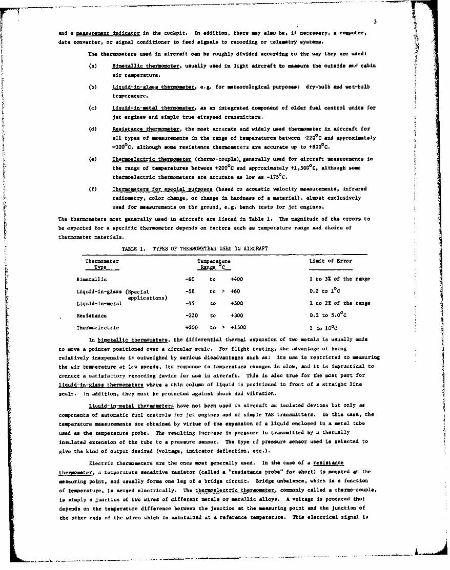
The thermometers most generally used in aircraft are listed in Table 1. The magnitude of the errors to

be expected for a specific thermometer depends on factors such as temperature range and choice of

thermometer materials.

TABLE 1. TYPES OF THERMOWTERS USED IN AIRCRAFT

Thermometer Temperature Limit of ErrorType Range UC

Bimetallic -60 to +400 1 to 3Z of the range

Liquid-in-glass (Special -58 to > +60 0.2 to 1°Capplications)

Liquid-in-metal -35 to +500 1 to 2Z of the range

Resistance -220 to +300 0.2 to 5.0°C

Thermoelectric +200 to > +1500 1 to 100C

In bimetallic thermometers, the differential thermal expansion of two metals is usually made

to move a pointer positioned over a circular scale. For flight testing, the advantage of being

relatively inexpensive is outweighed by serious disadvantages such as: its use is restricted to measuring

the air temperature at :cw speeds, its response to temperature changes is slow, and it is impractical to

connect a satisfactory recording device for use in aircraft. This is also true for the most part for

liquid-in-glass thermometers where a thin column of liquid is positioned in front of a straight line

scale. In addition, they must be protected against shock and vibration.

Liquid-in-metal thermometers have not been used in aircraft as isolated devices but only as

components of automatic fuel controls for jet engines and of simple TAS transmitters. In this case, the

temperature measurements are obtained by virtue of the expansion of a liquid enclosed in a metal tube

used as the temperature probe. The resulting increase in pressure is transmitted by a thermally

insulated extension of the tube to a pressure sensor. The type of pressure sensor used is selected to

give the kind of output desired (voltage, indicator deflection, etc.).

Electric thermometers are the ones most generally used. In the case of a resistance

thermometer, a temperature sensitive resistor (called a "resistance probe" for short) is mounted at the

measuring point, and usually forms one leg of a bridge circuit. Bridge unbalance, which is a function

of temperature, is sensed electrically. The thermoelectric thermometer, commonly called a thermo-couple,

is simply a junction of two wires of different metals or metallic alloys. A voltage is produced that

depends on the temperature difference between the junction at the measuring point and the junction of

the other ends of the wires which is maintained at a reference temperature. This electrical signal is

fl4then converted,using a sensitive ammeter, or by using a reference voltage and a compensa.tor, into thecorremponding temperature value. Since both types of ".ectric thermometers can be used for practically

all possible problems of temperature measurement In aircraft with a great degree of accuracy, flexibility,

sad reliability, and since the output can be easily prepared for recording and/or telemetry, they areused almost exclusively in flight tests. For these reasons, only these two types will be discussed in

greater detail in the following sections.

'rhe special-purpose thermometers include the temperature sensitive materials whose color depends

upon the highest temperature to which it has been exposed. There are even certain types which go througha multiple color change and can indicate up to four different temperature levels (cf. Section 6.1.4).

Mechanical temperature indicators are also used on occasion in engine tests. In this case, the change in

hardness of a material is a measure of the maximum temperature reached. Opia eprtuemaueet

are often made, in research and development tests, of the hot gases in combustion chambers and exhaust

streams. They have the advantages that no probes are mounted in the gas stream and hence gas flow and

temperature distributions are not disturbed, the possibility of thermometer damage and parts entering an

engine is minimizedand almost inertialess recordings are feasible. Some of the instruments can be usad

to obtain a measurement of the temperature distribution In the gas stream. However, this technique has

not yet been extended to in-flight applications.

There is a close relationship between thermometers and hot-wire anemometers which, ir' addition

to measuring the speed of the gas stream, can also be used at times to measure the temperature. This

measurement principle is based on the convective heat loss of an electrically heated wire mounted in a gas

stream. There are, however, many problems when using them as thermometers. Acoustic thermometers must

also be mentioned. These thermometers measure sound velocity as a function of the temperature. There

is little information on their use in aircraft.

Novel temperature probes such as specially-cut quartz crystals, temperature sensitive condensors,

etc. are often used in temperature measurements. Until now, however, no models of these devices have

been produced that are suitable for the measurement conditions in aircraft. The successful trials of a

Fluidic-TAT-probe up to Hach 6.7 in an X-15 aircraft are reported. It can be assumed that in the next

few years, "digital probes" of this sort, which do not produce a genuine digital signal, but rather a

variable frequency which can easily be converted to digital form, will come into use.

Almost all temperature measurements in aircraft are relative measurements, i.e. the indicators

give the temperature of an object relative to the melting point of ice measured in 0 C, and seldom theabsolute temperature in 0K. In special flight tests two temperature probes of the same type are mountedat different measuring points and connected differentially to the same measuring instrument, therebygiving the difference between Nwo temperatures AT in OC. The rate of change of temperature

may also be measured, In which case, two temperature probes with different time constants are connecteddifferentially at the same measuring point and to the same measuring instrument to indicate the ratethat the temperature is increasing or decreasing (A~T/At in + 0 C/min).

2. RES ISTANICE TEMPERATURE MEASUREMENTS

2.1. Resistance Probes

Metals, I.&. electrical conductors, are crystal structures that are composed of the corresponding

metal ions, i.e. of atoms whose valence electrons* have been freed by Brownian movement. When a voltage

is applied, a directional flow of free electrons is superimposed on this random motion. The electrons

collide with each other and with ions of the crystal lattice (which oscillate about an equilibrium position)

and thereby impede the flow, i.e. generate electrical resistance. As the conductor heats up, the

oscillations of the electrons and ions increase, i.e. resistance increases with temperature. The increase

in resistance in ferroelectric ceramics and the so-called "cold conductors" is much greater than in

metals.

*Valence electron -the electron in the outermost electron shell, which is bound only very loosely

to the atom.

In some types of the so-called "semiconductors", the valence electrons are bound more stronglyto the atoms and are freed only at higher temperatures so that the flow increases with the temperature(when voltage is applied), since acre electrons can join the flow of the current. In other words, theresistance decreases as the temperature increases. These semiconductors which are used as temperature

sensitive resistors are, therefore, also called "hot conductors".

In general, both phenomena mentioned above (increase or decrease in resistance withincrease in temperature) take place simultaneously, but generally one of the processes is predominant.However, certain metal alloys, the so-called "constant resistance alloys", can be produced which exhibit

no appreciable change of resistance with temperature over a rather wide temperature range.

The useful temperature range of a resistance probe is determined by the magnitude of thetemperature sensitivity,, cheamical reactions (heavy oxidation or reduction), permanent changes in thecrystal structure, etc. At very high temperatures, it is important to note that all insulators (e.g. glassabove 55000) become electric conductors (due to the release of all the valence electrons), and all

materials lose their impermeability to gas (important for shield tubes).

The slope of the R/T curve (resistance over temperature) can be expressed as a change inresistance AR per change in temperature AT of 1 C, or for purposes of comparison as the temperaturecoefficient a, i.e. as the relative change in resistance AR/R per CC, according to the equations:

AR R " AT and (1)x

&V (i/R x -AT) (2)

In practice, a (multiplied by 100) is usually expressed in Z/°C, and a is positive if

resistance increases with temperature, but negative if resistance decreases with temperature. Althougha is usually treated as a constant, in reality it bears a non-linear relation to temperature, and agiven value of a is exact at only one value of R.,

It is characteristic of temperature sensitive resistors that they are passive elements, andthat a current must be sent through them (e.g. in a bridge circuit) which can perceptibly heat up theresistor through the "Joule effect", causing a self-heating error. The definition of the "sensitivity"

of a temperature probe as the relationship between the variation in the output voltage AE for avariation in temperature AT of 10C for purposes of comparison with active temperature probes(therno-couples, which generate voltage of themselves) is very misleading. This applies especially

when measuring in media with a poor thermal conductivity (air or other gases, etc.), and when not allthe conditions art named, such as permissible self-heating error, magnitude of the probe resistance,

circuit design, type and velocity of the medium, etc.

In the following, Rx generally expresses the resistance value of an element at any temperature

Tx s and RxN is the value at a temperature TV Rx2 at T2, but Ro is the value at 0C, R2 thevalue at +250C, etc.

2.1.1 Elements with Positive Temperature Coefficients

Temperature probes of pure platinum wire were selected an the international standard fortemperature measurements between the boiling point of liquid oxygen (-182.970C) and the malting point

of antimony (+630.5 0 C),since the resistance-to-temperature ratio of pure platinum wire in an annealed andstrain-free state is especially stable and reproducible. The temperature coefficient increases rapidlyfrom zero at approximately 10°K (-2630C), reaches a maximum (0.422/OC) at approximately 30°K (-243°C)and then gradually decreases as the temperature is increased (Figures 4 and 5). The upper tempezature

limit for continuous operation is approximately 800°C (for short-term applications, 1,1000C). Tabulardata for the resistance values of coiled platinum wire elements as a function of temperature are found,e.g. for elements where R. - 100 ohms, in DIN 43760 (Reference 70). For elements where R° - 500 ohms,the values for N - 100 ohms should be multiplied by 5; where Ro -a50 ohm, the values should be halved,etc. Platinum with only a relatively high degree of purity is often used in various aeronautical devices,

and especially in total temperature probes, in order to obtain minor variations in H/T values;

these are set forth in MIL-P-25726 3 ASG and HIL-P-27723A. Platinum probes for aircraft are usuallymanufactured with a resistance R.o of 50 or 500 ohms in the U.S.A. However, other values are also used,

6

e.g. 100 ohms in Germany and France, and 200 or 700 ohms in Sweden. The deviations from the

corresponding standard R/T curves are generally lees than +l1C (cf. also Section 5.2.4).

In special cases, e.g. when measuring surface temperatures, elements are also used in the form

of coated platinum foil. The R/T curve is less predictable for platinum foil, but is dependent on

the thickness of the foil and must be found by individual calibrations (Reference 71).

Temperature probes made of nickel can be used in the temperature range from -190 to +180 0 C.V It is less expensive than platinum and has a somewhat higher temperature coefficient which increases as

the temperature is raised, but is also less stable. Above +180C it changes its interral structure as it

approaches the Curie point, so that its R/T curve can no longer be reproduced. Tables giving the data

on resistance values R. as a function of temperature can be found in DIN 43760 (Reference 70) where

R = 100 ohms or in MIL-B-7258 where Ro = 1,200 ohms. Probes for which R 0 is listed as 90.38 ohms are

actually composed of a temperature sensitive element for which R0 is approxsmately 60 ohms and a

V aeeries,30.38 ohm resistor housed in the base of the probe. The resulting R/T curves differ from those

of the other probes for this reason and is given in MIL-B-7990A (Figures 4 and 6). For the same reason,

approximately 30 ohms must be subtracted when determining the Joule heating in this type of probe. Other

resistauce values, e.g. 90 ohms, can be found in use in the UK. Since the temperature coefficient of

nickel increases with temperature, the N/T curve can be made more linear by connecting a resistor inparallel with R. (cf. examples in Figure 6). A shunt resistor approximately 3.6 times greater than

the average value of 1x for the range provides reasonable linearity but appreciably decreases the

slope of the characteristic curve. Anothrr resistor in series with the parallel combination is often

necessary for bridge design purposes, and further reduces the slope. The reduced slope of the corrected

curve naturally must be take. into consideration when measurements are made.

Copper of all the known metals has the temperature coefficient with the best linearity over an

extremely wide temperature range, however, it is not used for temperature probes in aircraft for various

reasons. Its temperature characteristics can, unfortunately, result in variable line resistance in theprobe conductorssthis is especially troublesome in probes with low resistance.

Silicon semiconductor elements are available that have a higher positive temperature coefficient

than metals and are suited for a temperature range from approximately -70 to +176 0 C. The variation in a

for the individual types is rather broad, however. Their R/T curve is practically linear over the

given range (Figure 7). There is as yet no data on the long-term stability of the material.

Occasionally, elements of a farroelectric ceramic, the so-called cold conductors, also calledPTC resistors*, are used. They consist primarily of sintered barium titanate with metallic oxides andhave a very high temperature coefficient, depending on their composition, over narrow temperature ranges

between approximately +20 and +160 0 C (Figure 7). At low temperatures, the resistance value is low,e.g.

40 ohms, and varies only slightly with changes in temperature. When the Curie temperature is reached,

barrier layers are formed in the ceramic and the resistance increases exponentially with temperature bymore than three orders of magnitude. Above this usable range with large temperature coefficients, a

again decreases and sometimes even becomes negative. The initial resistance R2 5 , at 250C, lies between

3 and 1,000 ohms depending on the model. The variation between probes of the same type necessitates

individual calibrations. For rough measurements within small temperature ranges, the high temperature

coefficient permits the fabrication of relatively inexpensive, but quite sensitive, resistance thermometers.

There has not been enough experience in using them in aircraft to make statements on their stability,

aging, etc. (Reference 73).

2.1.2 Resistance Materials with Negligible Temperature Coefficients

Resistors of manganin (a Cu-Mn-Ni alloy) wire exhibit a nearly constant resistance value over a

wide range of temperatures. For this reason, this material is very suitable for manufacturing precision

resistors, which are necessary in the bridge circuits for temperature probes. The temperature coefficient

of constantan (a Cu-Ni alloy) wire is also close to zero, but exhibits a large thermoelectric effect when

used with copper, so that it is not recommended for use in resistance-temperature measurements.

*PTC - positive temperature coefficient.

7

2.1.3 Elements with Negative Temperature Coefficients

Semiconductors with negative temperature coefficients, the so-called thermistors (also called

Newi, Urdox, Thernewid or NTC resistors) are made of sintered ceramics, usually of mixtures of metal oxides,

e.g. iron, manganese, nickel, cobalt, copper, titanium or uranium oxide, preferably with values for

between 100 ohms and 100 kilohms. As is the case with most semiconductor probes, the same types do not

have identical temperature coefficients, so that a recalibration of the thermometer arrangement is usually

necessary when the probe is changed. However, there are selected models with very close tolerances and

probe assemblies that are directly interchangeable. In the latter case, a resistance (e.g. 3 kUG) is

applied in series with the probe and a resistance (e.g. 30 ks2) in parallel with this series arrangement

so that the resultant R/T curve exhibits a somewhat lower temperature coefficient than the element

itself. The range of applicability of thermistors usually lies between the limits of approximately -100 0 C

and +300 0 C, but an individual type rarely has a temperature range greater than 100 to 2500 C. Larger

measurement ranges often require a change of the bridge or different types of probes. Special types of

thermistors are available where the lower limit at the present time is approximately 10°K (approximately

-263°C). and the upper limit is approximately +400 to +4500 C.

Because of their small size, thermistors are especially suitable for point measurements or for

determining the temperature gradients between closely spaced points.

The resistance curve of thermistors with respect to temperature is approximately exponential

(Figure 7) and can be expressed by the equation

R= a • •b/T (3)

where "a" (in ohms) is a constant determined by the form and material and "b" (in 0 K) is a constant

determined primarily by the materiai. The temperature coefficient can be described by the equation

-AR/(R 25 A !T) - -b/T 2 (3a)

and is typically -3 to -5%/°C (depending on temperature T). In specifications, the resistance is5 s

usually given (i.e. R at 25 C or 2980 K), as well as the b-value or the resistance ratio Rxl/Rx2 "

given temperature values T1 and T2 (in oK). The connection between both definitions is expressed by

the equation

Rx2 - R xl - leT2 ) (3b)

This equation enables us to calculate the resistance value R for any value of T2 (Reference 78).

The advantage of the large temperature coefficient, which is approximately 10 times greater

than those of Pt and Ni resistances, can only be completely exploited when measurements are made in

good thermal conductors. The self-heating in air is very great so that very small measuring currents

must be used in the probe. As a result of the differences in construction of beads or rods in contrast

to wire-wound resistors, the fact that the currant flow in the material is not uniform when there is a

change in temperature or when there are large currents mast be considered for all types of semiconductors,

since heat can only be absorbed or released at the surfaces*. For voltages of less than 1 volt at the

probe, the contact resistance at the pigtails must also be considered, since there is a relationship

between the voltage and the contact resistance (Riference 78). Probes supplied with inexpensive connectors

often cannot be used to measure aIr teuperatures for exactly this reason.

In order to measure extremely low temperatures (Figure 8), elements of doped germanium can be

used (in addition to the special low-temperature thermistors mentioned previously) in the range from

approximately 1 to 400 K (approximately -272 to -2330C). Also carbon resistors can be used in the range

from approximately 0.1 to 15 or 20 0 K. Above approximately 230K (-250°C) these materials are not as good

as platinum, both with respect to the value of their temperature coefficients and their stability, so

*It could be that "recovery factors > 1.0" found in air with thermistors are based on this effect

(cf. Section 4.3.3.2).

8

they will not be discussed further in detail.

2.1.4 Construction of Resistance Elements

Because of the different requirements (time constants, ability to withstand vibration orchemical corrosion, etc.), or their relative importance in any individual application, constructiontechniques vary considerably. Figure 9a shove a so-called open-viro element in which a platinum wire

is wound on a perforated coil form. Therefore, the wire is in direct contact with the Sga orliquid whose temperature is to be measured. This lesmnt generally has an excellent response time, asmall conductiou error, and a small self-heating error. The gases or liquids must not be corrosive orconductive, nor leave sediments behind. In the case of tubular elements (Figures 9b and 9c) theresistance wire is protected and withstands high pressures, fluid speeds and vibrations, and is lesseasily damaged by small foreign bodies. In the more expensive model, Figure 9b, the wire is harmatically

sealed between two platinum tubes, whereas in the modal shown in Figure 9c, the wire has an organic coatingand is embedded in ceramic. Since both the inside and outside of the tube is exposed to the medium, botha good time constant and good protection of the resistance wire is obtained. Figure 9d shows a ceramiccoated miniature element which must be protected against mechanical damage by a wire net or cylinder,but has a relatively small time constant as a result of its small size. Too high bridge currents canoverheat this type of element. The well-type elements, Figures 9e, f and g, protect best against fastflowing, electrically conductive or corrosive liquids, even when there are heavy oscillations, by

enclosing the resistance wire inside of a stainless steel or platinum tube which is sealed at both ends.These types are primarily used as top-sensitive elements for measurements in solid bodies and stem-

sensitive elements for measurements in liquids and gases. The well-type elements that require a solid coreinherently have very high time constants. In stem-sensitive models without a core (Figure 9g), the timeconstants are sharply reduced. In the case of flat elements (Figures 9h and i, showing elements ofquadrilateral form*) the resistance wire is embedded in insulating material and housed in a thin metal

chamber (stainless steel, aluminum, platinum etc.). In some models, a metallic layer Is vaporizee in theinsulation material, which,however, is quite subject to mechanical damage. Flat elements are mainly used

to measure surface temperatures. For this purpose, there are special models in which the resistance

wire is sandwiched between two flexible pieces of resin-impregnated glass paper so that it can be woundaround small tubes.

The widely different types of element construction resultamong other things, from the fact that

the thermal expansion of the resistance wire, insulation, coil forms and chambers must be as equal asSpossible in order to prevent changes in the resistance by elongation (mechanical stress) of the resistance

wire (similar to the effect of a wire strain gauge). Otherwise, the calibration of a probe element wouldbe almost or completely non-reproducible. The required vibration resistance and the resistance value,

I.e. the required wire length, also are important considerations. Semi-conductor elements are manu-

fsctured in very different forms, e.g. as spheres (Figure 9k) or disks, spheres embedded in a glass bead,

layered glass laminates, or even in special mountings (Figure 10), and are characterized by their small

se. Specal models for use in aircraft have not yet been developed.

2.1.5 Construction of Resistance Probes

When a resistance element, which is usually manufactured without a mounting and with loose lead

wires, is provided with a socket, a protective shield or a housing, and a radiation shield, it is known asa temperature probe.

The well-type probe is one of the most common types of construction. The types that are intendedfor temperature moeasurements in liquids and gases are made up of a long tube,a threaded base and a socketfor the electric connection. The resistance element is housed in the rod-shaped protective tube and is

so constructed that the temperature changes on the surface of the cylinder have sore effect than thoseat the upper end (stem-sensitive type.). Examples are shown in Figures 12a and b. There are models inwhich a second concentric protective tube can be attached (as can be seen on the bimetallic thermometer

in Figure 11). This serves to reduce the radiation error, to channel the flow between the protective

tube and the element so that the recovery factor becomes larger, and to decrease the time constant with

*Cf. also Figure 94.

9

respect to the temperature changes of the liquid or gas (see Section 4.3). For the saes reason,

certain types are given a right-angle bend (Figures 12c and d) so that the air current flows parallel to

the temperature sensitive part of the surface. They are also manufactured with an additional radiation

shield. Another type of construction, which is only used when measuring air temperatures, is the

knfeedge-robe, that is mounted perpendicular to the surface of the aircraft, but parallel to the air

flow (Figure 13b). Figure 13a shovs a type. which was earlier quite commo, that is equipped with aprotective housing that also serves to a certain extent as a radiation shield. A similar structure is

the flush-bulb (Figure 14). It is mounted flush with the airplane skin, but thermally insulated from it.

The air flows parallel to its surface. This probe provides a relatively inexpensive method of measuring

the air temperature, but the measurement accuracy decreases quickly as the speed is increased, even when

the mounting location is carefully chosen, since the temperature is measured in the boundary layer of the

aircraft (cf. Sections 4.3 and 6.4.2).

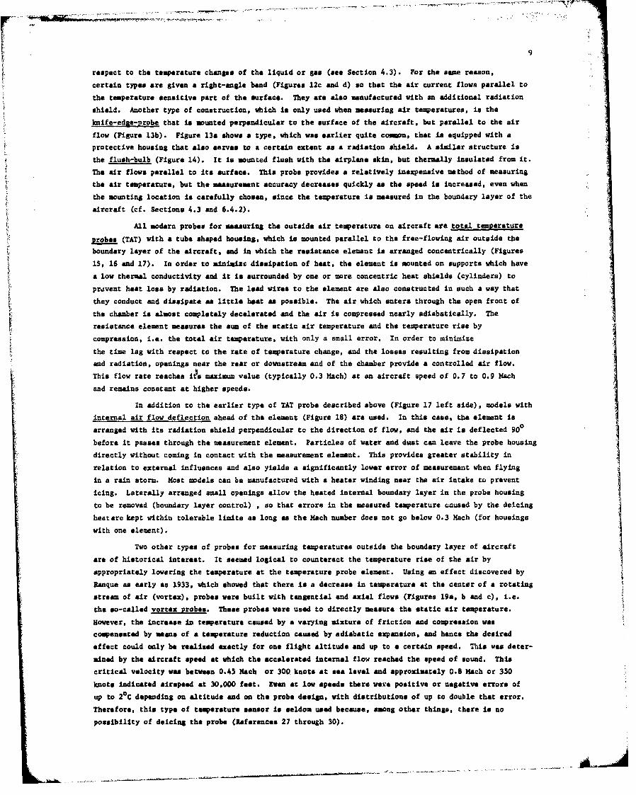
All modern probes for measuring the outside air temperature on aircraft are total temperature

probes (TAT) with a tube shaped housing, which Is mounted parallel to the free-flowing air outside theboundary layer of the aircraft, and in which the resistance element is arranged concentrically (Figures

5 15, 16 and 17). In order to minimiaze dissipation of heat, the element Is mounted on supports which have

a low thermal conductivity and it Is surrounded by one or more concentric heat shields (cylinders) to

pravent heat loss by radiation. The lead wires to the element are also constructed in such a way that

they conduct and dissipate as little heat as possible. The air which enters through the open front of

the chamber is almost completely decelerated and the air is compressed nearly adiabatically. The

resistance element measures the sum of the static air temperature and the temperature rise by

compression, i.e. the total air temperature, with only a small error. In order to minimize

the time lag with respect to the rate of temperature change, and the losses resulting from dissipation

and radiation, openings near the rear or downstream end of the chamber provide a controlled air flow.

This flow rate reaches itts maximum value (typically 0.3 Mach) at an aircraft speed of 0.7 to 0.9 Mach

and remains constant at higher speeds.

In addition to the earlier type of TAT probe described above (Figure 17 left side), models with

internal air flow deflection ahead of the element (Figure 18) are used. In this case, the element is

arranged with its radiation shield perpendicular to the direction of flow, and the air is deflected 900

before it passes through the measurement element. Particles of water and dust can leave the probe housing

directly without coming in contact with the measurement element. This provides greater stability in

relation to external influences and also yields a significantly lower error of measurement when flying

in a rain storm. Most models can be manufactured with a heater winding near the air intake to prevent

icing. Laterally arranged small openings allow the heated internal boundary layer in the probe housingto be removed (boundary layer control) , so that errors in the measured temperature c~aused by the deicing

heat are kept within tolerable limits as long as the Mach number does not go below 0.3 Mach (for housings

with one element).

are ofhsorlithertyest It seemed logeauical toecuneractuthes otemierature budris ofatear byaicrf

aeohitworia ontheryest of proeseormeasuringa tempuneracthteprtures outidete budrlae ofth aircraf

appropriately lowering the temperature at the temperature probe element. Using an effect discovered by

Ranque as early as 1933, which showed that there is a decrease in temperature at the center of a rotating

stream of air (vortex), probes were built with tangential and axial flows (Figures 19a, b and c), i.e.

the so-called vortex probes. These probes were used to directly measure the static air temperature.

However, the increase In temperature cauwed by a varying mixture of friction and compression was

compensated by means of a temperature reduction caused by adiabatic expansion, and hence the desired

effect could only be realised exactly for one flight altitude and up to a certain speed. This was deter-

mined by the aircraft speed at which the accelerated internal flow reached the speed of sound. This

critical velocity was between 0.45 Mach or 300 knots at sea level end approximately 0.8 Mach or 350

knots indicated airspeed at 30,000 feet. Even at low speeds there were positive or negative errors of

up to 2oC depending on altitude and on the probe design, with distributions of up to double that error.

Therefore, this type of temperature sensor is seldom used because, amiong other things, there is no

possibility of deicing the probe (References 27 through 30).

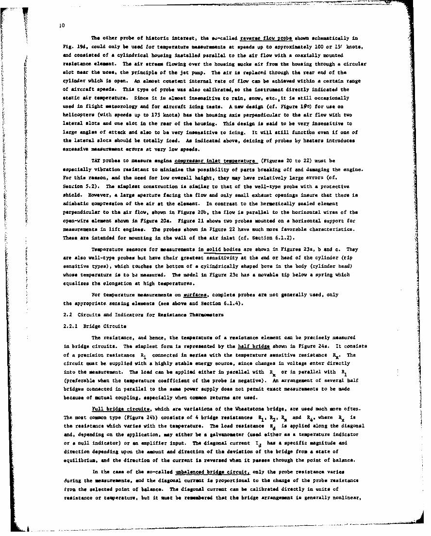
10 ,cudol eue o eprtr esrmnt tsed pt prxmtl 0 r1(hos

The other probe of historic interest* the eo-called reverse. flow probe shown schematically in

end consisted of a cylindrical housing installed parallel to the air flow with a coaxially mounted

resistance element. The air stress flowing over the housing sucks air from the housing through a circular

slot near the nose, the principle of the jet pump. The air is replaced through the rear end of the

cylinder which is open. An. almost constant internal rate of flow can be achieved within a certain range8 ~of aircraft speeds. This type of probe was also calibrated, so the instrument directly indicated the

static air temperature. Since it is almost insensitive to rain, snow, etc. ,it is still occasionally

used in flight meteorology and for aircraft icing tests. A new design (cf. Figure 19e) for use on

helicopters (with speeds up to 175 knots) has the housing axis perpendicular to the air flow with two

lateral slots and one slot in the rear of the housing. This design is said to be very Insensitive to

large angles of attack and also to be very insensitive to icing. it will still functilon even if one ofthe lateral slots should be totally iced. As indicated above, deicing of probes by heaters introduce$

excessive measurement errors at very low speeds.

TAT probes to measure engine compressor inlet temperature (Figures 20 to 22) must be

especially vibration resistant to minimize the possibility of parts breaking off and damaging the engine.

For this reason, and the need for low overall height, they may have relatively large errors (cf.Seacion 5.2). The simplest construction is similar to that of the well-type probe with a protective

shield. However, a large aperture facing the flow and only small exhaust openings insure that there is

adiabatic compression of the air at the element. In contrast to the hermetically sealed element

perpendicular to the air flow, shown in Figure 20b, the flow is parallel to the horizontal wires of theIopen-wire element shown In Figure 20a. Figure 21 shows two probes mounted on a horizontal support for

measurements in lift engines. The probes shown in Figure 22 have much more favorable characteristics.

These are intended for mounting in the wall of the air inlet (cf. Section 6.1.2).

Temperature sensors for measurements in solid bodies are shown in Figures 23a, b and c. Theyare also well-type probes but have their greatest sensitivity at the end or head off the cylinder (tip

sensitive types), which touches the bottom of a cylindrically shaped bore in the body (cylinder head)

whose temperature is to ba measured. The model in Figure 23c has a movable tip below a spring which

equalizes the elongation at high temperatures.

For temperature measurements on surfaces, complete probes are not generally used, only

the appropriate sensing elements (see above and Section 6.1.4).

2.2 Circuits and Indicators for Resistance Thermometers

2.2.1 Bridge Circuits

The resistance, and hence, the temperature of a resistance element can be precisely measured

in bridge circuits. The simplest form is represented by the half bridge shown in Figure 24a. It consists

of a precision resistance R1. connected in series with the temperature sensitive resistance R.A. The

circuit must be supplied with a highly stable energy source, since changes in voltage enter directlyinto the measurement. The load can be applied either in parallel with R or in parallel with R,

bridges cc~nnected in parallel to the same power supply does not permit exact measurements to be made

because of mutual coupling, especially when commo returns are used.

Full bridae circuits, which are variations of the Wheatstone bridge, are used much more often.

The most cmon type (Figure 24b) consists of 4 bridge resistances Rl. R2, P- and R 4, where Rx is

the resistance which varies with the temperature. The load resistance R d is applied along the diagonal

and, depending on the application, may either be a galvanometer (used either as a temperature indicator

or a null indicator) or an amplifier input. The diagonal current I d has a specific magnitude end

direction depending upon the amount and direction of the deviation of the bridge from a state of

equilibrium, and the direction of the current In reversed when it passes through the point of balance.

In the case of the so-called unbalanced bridge circuit, only the probe resistance varies

luring the measurements, and the diagonal current is proportional to the change of the probe resistance

from the selected point of balance. The diagonal current can he calibrated directly in units of

resistance or temperature, but it must be remembered that the bridge arrangement is generally nonlinear,

i.e. an absolutely linear calibration can only be obtained under certain conditions.

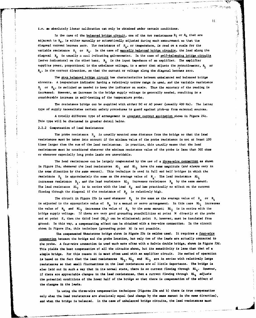
In the case of the balanced bridge circuit, one of the two resistances RI or R4 that are

adjacent to R1, is either manually or automatically adjusted during each measurement so that thediagonal current becomes zero. The resistance of R.,i or temperature, is read on a scale for the

variable resistance R or R. In the case of manually balanced bridge circuits, the load along the

diagonal Rdis usually a nuii indicating galvanometer. In the case of self-balancing bridge circuits

(servo indicators) on the other hand,, Rd is the input impedance of an amplifier. The amplifier

supplies power, proportional to the unbalance voltage, to a motor that adjusts the potentiometer, R, or

R, in the correct direction, so that the current or voltage along the diagonal becomes zero.

The step balanced bridge circuit has characteristics between unbalanced and balanced bridge

circuits. A temperature indicator having a relatively narrow range is used, and the variable resistance

Ror R , is switched as needed to keep the indicator on scale. Thus the accuracy of the reading is

increased. However, an increase In the bridge supply voltage is generally needed, resulting in a

considerable increase in self-heating of the temperature probe.

The resistance bridge can be supplied with either DC or AC power (usually 400 Hz). The latter

type of supply necessitates certain safety procedures to guard against pick-up from external sources.

A totally different type of arrangement is constant current excitation shown in Figure 24c.

This type will be discussed in greater detail below.

2.2.2 Compensation of Lead Resistances

The probe resistance R is usually mounted some distance from the bridge so that the lead

resistances must be taken into account if the minimum value of the probe resistance is not at least 100

times larger than the sum of the lead resistances. In practice, this usually means that the lead

resistances must be considered whenever the minimum resistance value of the probe is less than 300 ohms

or whenever especially long probe leads are unavoidable.

The lead resistances can be largely compensated by the use of a three-wire connection as shown

in Figure 25a, whenever the lead resistances RL1 and EL3 have the same magnitude (and always vary in

the same direction by the same amount). This technique is used in full and half bridges in which the

resistance R I is approximately the same as the average value of R x. The lead resistance EL1increases resistance R,, and the lead resistance RL3 increases resistance R~ by the same amount.

The lead resistance EL2 is in series with the load Rd and has practically no effect on the current

flowing through the diagonal if the resistance of Rd is relatively high.

The circuit in Figure 25b is used whenever R 4 is the same as the average value of R X or R 4is adjusted to the appropriate value of R. by a manual or servo arrangement. In this case RL1 increases

the value of Rt4 and RL3 increases the value of It, by the same amount; RL2 is in series with the

bridge supply voltage. If there are very good grounding possibilities at point M directly at the probe

and at point E, then the third lead (EL2) can be eliminated; point N, however, must be insulated from

ground. In this way, a compensating effect can be obtained with a two-wire connection. In the circuit

shown in Figure 25a, this technique (grounding point H) is not possible.

The compensated Wheatstone bridge shown in Figure 25c is seldom used. It requires a for-wire

connection between the bridge and the probe location, but only two of the leads are actually connected to

the probe. A four-wire connection is used much more often with a Kelvin double bridge, shown in Figure 25d.

This yields the best compensation of all the circuits shown, but its sensitivity is less than that of a

simple bridge. For this reason it is most often used with an amplifier circuit. Its method of operation

is based on the fact that the lead resistances EL1, RL 2 and EL 3 are in series with relatively large

resistances so that small fluctuations in the lead resistances are of little importance. The bridge is

also laid out in such a way that in its normal state, there is no current flowing through RL4. oevrif there are appreciable changes in the lead resistances, then a current flowing through RL4 adjusts

the potential conditions of the lower half of the bridge so that there is compensation of the effect of

the changes in the leads.

in using the three-wire compensation techniques (Figures 25& and b) there is true compensation

only wham the lead resistances are absolutely equal (and change by the esam amount in the same direction),

and when the bridge is balanced. In the case of unbalanced bridge circuits, the lead resistances must

12

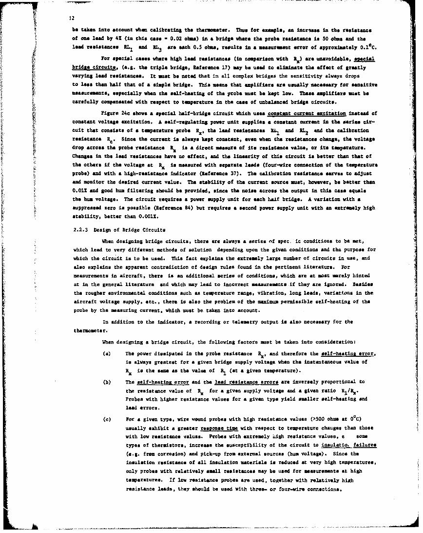
be taken into account when calibrating the thermometer. Thus for example, an incr*ese in the resistance

of one lead by 41 (in this case - 0.02 ohms) in a bridge where the probe resistance is 50 ohms and the

lead resistances RL1 and RL3 are each 0.5 ohms, results in a measurement error of approximately 0.1°C.

Z For special cases where high lead resistances (in comparison with Rx) are unavoidable, special

bridge circuits, (e.g. the triple bridge, Reference 17) may be used to eliminate the effect of greatly

varying lead resistances. It mset be noted that in all complex bridges the sensitivity always drops

to lees than half that of a simple bridge. This means that amplifiers are usually necessary for sensitiveC'a

measurements, especially when the salf-heating of the probe must be kept low. These amplifiers must be

"carefully compensated with respect to temperature in the case of unbalanced bridge circuits.

Figure 24c shovs a special half-bridgo circuit which uses constant current excitation instead of

constant voltage excitation. A self-regulating power unit supplies a constant current in the series cir-

cuit that consists of a temperature probe R., the lead resistances RL1 and RL2 and the calibration

resistance Rc. Since the current is always kept constant, even when the resistances change, the voltage

drop across the probe resistance Rx is a direct measure of its resistance value, or its temperature.t Changes in the lead resistances have no effect, and the linearity of this circuit is better than that of

the others if the voltage at Rn is measured with separate leads (four-wire connection of the temperature

probe) and with a high-resistance indicator (Reference 37). The calibration resistanoe serves to adjust

and monitor the desired currant value. The stability of the current source must, however, be better than

0.011 and good hum filtering should be provided, since the noise across the output in this case equals

the hum voltage. The circuit requires a power supply unit for each talf bridge. A variation with a

I •suppressed zero is possible (Reference 84) but requires a second power supply unit with an extremely high

stability, better than 0.001%.

2.2.3 Design of Bridge Circuits

When designing bridge circuits, there are always a series nf spec. ic conditions to be met,

*. which lead to very different methods of solution depending upon the given conditions and thc purpose for

which the circuit is to be used. This fact explains the extremely large number of circuits in use, and

also explains the apparent contradiction of design rules found in the pertinent literature. For

measurements in aircraft, there is an additional series of conditions, which are at most merely hinted

at in the general literature and which may lead to incorrect measurements if they are ignored. Besides

the rougher environmental conditions such as temperature range, vibration, long leads, variations in the

aircraft voltage supply, etc., there is also the problem of the maximum permissible self-heating of the

probe by the measuring current, which must be taken into account.

In addition to the indicator, a recording or telemetry output is also necessary for the

thermometer.

When designing a bridge circuit, the following factors must be taken into consideration:

(a) The power dissipated in the probe resistance Re, and therefore the self-heating error,

is always greatest for a given bridge supply voltage when the instantaneous value of

Rt is the same as the value of R, (at a given temperature).

(b) The self-heating error and the lead resistance errors are inversely proportional to

the resistance value of Rx for a given supply voltage and a given ratio R1 1/R.

Probes with higher resistance values for a given type yield smaller self-heating and

lead errors.

(c) For a given type, wire wound probes with high resistance values (>500 ohms at 0C)

usually exhibit a greater response time with respect to temperature chauges than those

with low resistance values. Probes with extremely 4igh resistance values, e some

types of thermistors, increase the susceptibility of the circuit to insulatio. failures

(e.g. from corrosion) and pick-up from external sources (hum voltage). Since the

insulation resistance of all insulation materials is reduced at very high temperatures,

only probes with relatively small resistances may be used for measurements at high

temperatures. If low resistance probes are used, together with relatively high

resistance leads, they should be used with three- or four-wire connections.

13

(d) Since all bridge circuits are nonltnear, the bridge output voltage is always a

nonlinear function of the probe resistance. The latter, however, is also a nonlinear

function of the temperature. Nevertheless, when the bridge is designed appropriately,

a nearly linear indicator scale can be obtained, as long as the indicator range is not

extremely large.

(e) Bridges with recording or telemetry outputs should be designed so that the connected

equipment has as little effect as possible on the calibration of the circuit.

(f) Changes in the environmental temperature of the bridge should not have any effect.

This can be achieved by using bridge resistors of manganin wire and all the connecting

leads of copper wire. In certain cases, the bridge resistances can be made using a

copper wire section and a mangan$,n wire section. The use of constantan and othermetals. which in combination with copper generate an appreciable thermoelectric

voltage, must be avoided in all cases. Even the temperature sensitivity of the leads

connected to the bridge, including that of the instruments, amplifiers, etc., must bestudied and if necessary compensated for.

(g) The bridge supply voltage should be regulated to better than 0.12, since voltage changes

yield corresponding read-out errors. Exceptions are bridges with ratio meters, and

servo bridges.

(h) In addition to the requirements for high insulation resistances, extremely smallcontact resistances in plugs, switches, potentiometer slip rings, etc., the usual

environmental requirements for aircraft equipment, such as vibration resistance,

mast also be met.

When designing a circuit, it is therefore always necessary to compromise between requirements

that are to a certain extent contradictory.

2.2.3.1 Half Bridge Circuits

This circuit, which is usually used only for recording or telemetry purposes, consists

primarily of the probe resistance Rx and a series resistance R, (Figure 24a). The use of a three-wire

connection is possible, if R, is approximately equal to the mean value of Rx . For reasons mentioned

below, relatively high resistance probes are selected so that the effect of the leads is very small; in

this case, the magnitude of R, can be any selected value. If the load R which should be as high in

resistance as possible, is connected in parallel with Rl, the relationships are mere easily seen as

the magnitude of Rx varies. It must be taken into account that the polarity of the output voltagedepends on whether Rd is applied in parallel with R, or Rx, and also depends on whether the probetemperature coefficient is positive or negative.

In Figure 26a the ratio of the output voltage UA (across R1 ) to the supply voltage UB is

given as a function of the temperature, when nickel probes are used (the curves would be similar for

platinum probes). The useful change in the output voltage is relatively small for Case I but is

increased by selecting higher probe resistances and lower values for R 1/Ro (Case II). In Case II, a

relatively high bridge supply voltage UB was also selected. In order to prevent excessive self-heating

of the probe by the measuring current, the maximvu bridge voltage is determined by the maximum permissible

power generated in the probe.

Example (refer to Figure 26a):

Range of measurement = 0 to 100°C

Probe resistance at OeC R* (nickel element) a 100 ohms0

Dissipation constant in flowing water - 112 mW/°C

Permissible self-heating error = 0.2 0 C

Permissible power at the probe P w (112 . 0.2) - 22.4 mW - 0.0224 W

*When Ro - 100 ohms, the lead resistances will have a significant effect.

AU

14

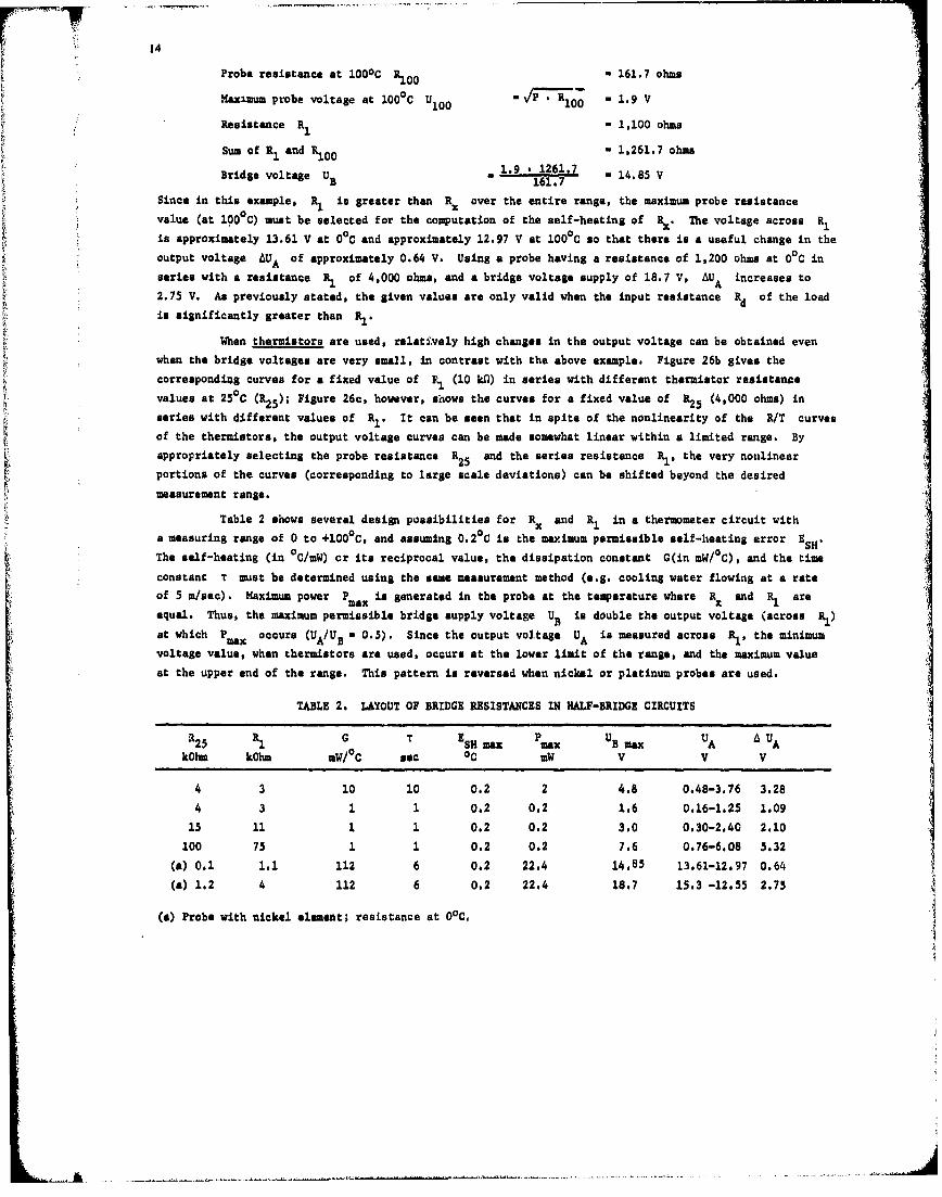
Probe resistance at 1000C O1 ... - 161.7 ohms

Maximum probe voltage at 100°C U10 0 = * - 1.9 V

Resistance R1 1,100 ohms

Sum of R and R1 00 n 1,261.7 ohmsBridge voltage U3 1.9 B 1261.7 14.85 V" 161.7 1.8 ,-

Since in this example, R, is greater than Rx over the entire range, the maximum probe resistance

value (at 100%C) must be selected for the computation of the self-heating of Rx. The voltage across R,

is approximately 13.61 V at 0°C and approximately 12.97 V at 100°C so that there is a useful change in the

output voltage WA of approximately 0.64 V. Using a probe having a resistance of 1,200 ohms at O°C in

series with a resistance 1 of 4,000 ohms, and a bridge voltage supply of 18.7 V. AUA increases to

2.75 V. As previously stated, the given values are only valid when the input resistance Rd of the load

is significantly greater than R1 .

When thermistors are used, relatively high changes in the output voltage can be obtained even

when the bridge voltages are very small, in contrast with the above example. Figure 26b gives the

correspondiag curves for a fixed value of B11 (10 kP) in series with different thermistor resistanne

values at 25°C (R2 5 ); Figure 26c, however, shows the curves for a fixed value of R2 (4,000 ohms) in

series with different values of R1 . It can be seen that in spite of the nonlinearity of the R/T curves

of the thermistors, the output voltage curves can be made somewhat linear within a limited range. By

appropriately selecting the probe resistance R2 5 and the series resistance K1 , the very nonlinearportions of the curves (corresponding to large scale deviations) can be shifted beyond the desired

measurement range.

Table 2 shows several design possibilities for R. and R1 in a thermometer circuit with

a measuring range of 0 to +1000C, and assuming 0.2 0C is the maximum permissible self-heating error ESH,

The self-heating (in 0 C/mW) cr its reciprocal value, the dissipation constant G(in mW/ 0C), and the time

constant T must be determined using the same measurement method (e.g. cooling water flowing at a rate

of 5 m/sac). Maximum power P is generated in the probe at the temperature where Rx and K1 are

equal. Thus, the maximum permissible bridge supply voltage UR is double the output voltage (across R)

at which Pmax occurs (UA/UB - 0.5). Since the output voltage UA is measured across Rl, the minimum

voltage value, when thermistors are used, occurs at the lower limit of the range, and the maximum value

at the upper end of the range. This pattern is reversed when nickel or platinum probes are used.

TABLE 2. LAYOUT OF BRIDGE RESISTANCES IN HALF-BRIDGE CIRCUITS

R2 5 R1 SG E lu max Pmax UB ax UA A UA

kOhm kOhm mW/OC sec 0C mW V V V

4 3 10 10 0.2 2 4.8 0.48-3.76 3.28

4 3 1 1 0.2 0.2 1.6 0.16-1.25 1.09

15 11 1 1 0.2 0.2 3.0 0.30-2.40 2.10100 75 1 1 0.2 0.2 7.6 0.76-6,08 5.32

(a) 0.1 1.1 112 6 0.2 22.4 14.85 13.61-12.97 0.64(a) 1.2 4 112 6 0.2 22.4 18.7 15.3 -12.55 2.75

(a) Probe with nickel element; resistance at O°C,

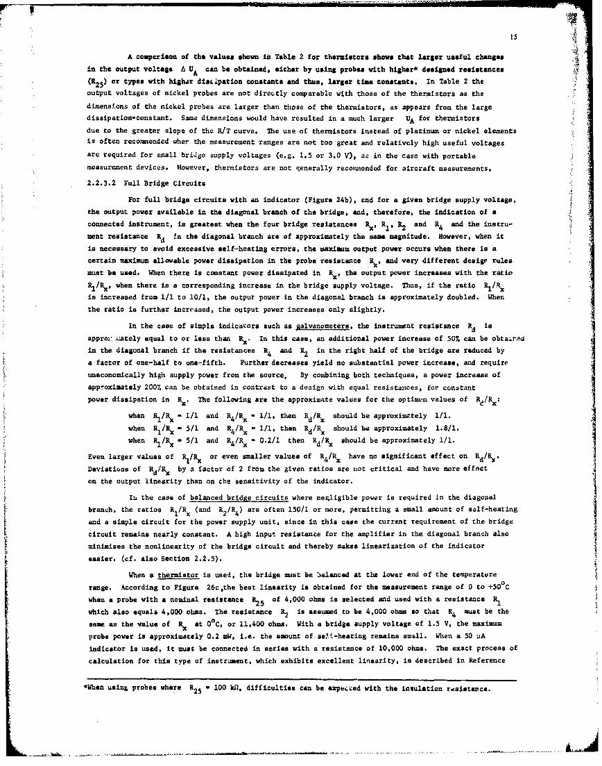
A comparison of the values shown in Table 2 for thermistors shows that larger useful changes

in the output voltage * UA can be obtained, either by using probes with higher* designed resistances

(R2 5 ) or types with higher dist~pation constants and thus, larger time constants. In Table 2 the

output voltages of nickel probes are not directly comparable with those of the thermistors as the

dimensions of the nickel probes are larger than those of the thermistors, as appears from the large

dissipation-constant. Same dimensions would have resulted in a much larger UA for thermistors

due to the greater slope of the R/T curve. The use of thermistors instead of platinum or nickel elements

is often recommended wher the measurement ranges are not too great and relatively high useful voltages

are required for small bridge supply voltages (e.g. 1.5 or 3.0 V), az in the case with portable

measurement devices. However, thermistors are not generally recommended for aircraft measurements.

2.2.3.2 Full Bridge Circuits

For full bridge circuits with an indicator (Figure 24b), and for a given bridge supply voltage,

the output power available in the diagonal branch of the bridge, and, therefore, the indication of a Aconnected instrument, is greatest when the four bridge resistances R., R1 , R2 and R4 and the instru-

ment resistance Rd n the diagonal branch are of approximately the same magnitude. However, when it

is necessary to avoid excessive self-heating errors, the maxinum output power occurs when there is a

certain maximum allowable power dissipation in the probe resistance R , and very different desigr rules

must be used. When there is constant power dissipated in Rx, the output power increases with the ratio

Rj/Rx, when there is a corresponding increase in the bridge supply voltage. Thus, if the ratio RlIx

is increased from 1/1 to 10/1, the output power in the diagonal branch is approximately doubled. When

the ratio is further increased, the output power increases only slightly.

In the case of simple indicators such as galvanometers, the instrument resistance Rd is

appror..uately equal to or less than R.. In this case, an additional power increase of 50% can be obtained

in the diagonal branch if the resistances R4 and R2 in the right half of the bridge are reduced by

a factor of one-half to one-fifth. Further decreases yield no substantial power increase, and require

uneconomically high supply power from the source. By combining both techniques, a power increase of

approximately 200% can be obtained in contrast to a design with equal resistances, for constant

power dissipation in Rx. The following are the approximate values for the optimum values of Rd/Rx:

when Rl/Rx - 1/1 and R4 /R - 1/1, then Rd/R should be approximntely 1/1.when R/Rx = 5/1 and R4/Rx = 1/1, then R x/R should be approximately 1.8/1.

we R/R-5/1 andR/R -1,thnR/R should be approximately 1./1.when Rl/R - 5/1 and R4/R = 0.2/1 then Rd/Rx should be approximately 1/.

Even larger values of Rl/Rx or even smaller values of /R4 have no significat effect on xdX.

Deviations of Rd/Rx by a factor of 2 from the given ratios are not critical and have more effect

on the output linearity than on the sensitivity of the indicator.

In the case of balanced bridge circuits where negligible power is required in the diagonal

branch, the ratios R,/R (and R2 /R4 ) are often 150/1 or more, permitting a small amount of self-heating

and a simple circuit for the power supply unit, since in this case the current requirement of the bridge

circuit remains nearly constant. A high input resistance for the amplifier in the diagonal branch also

minimizes the nonlinearity of the bridge circuit and thereby makes linearization of the indicator

easier. (cf. also Section 2.2.5).

When a thermistor is used, the bridge must be balanced at the lower end of the temperature

range. According to Figure 26cthe best linearity is obtained for the measurement range of 0 to +50 0 C

when a probe with a nominal resistance R25 of 4,000 ohms is selected and used with a resistance R1

which also equals 4,000 ohms. The resistance R2 is assumed to be 4,000 ohms so that R4 must be the

same as the value of Rx at O°C, or 11,400 ohms. With a bridge supply voltage of 1.5 V, the maximum

probe power is approximately 0.2 mW, i.e. the amount of se.!-heating remains small. When a 50 PA

indicator is used, it must be connected in series with a resistance of 10,000 ohms. The exact process of

calculation for this type of instrument, which exhibits excellent linearity, is described in Reference

*When using probes where R2 5 - 100 kIQ, difficulties can be expected with the invulation reuistance.

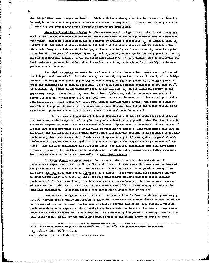
4V16

80. Larger measurement ranges are hard to obtain with thermistors, since the improvement in linearity

by applying a resistance in parallel with the t'.ermiastor is very small. In this case, it is preferable

to use a silicon semiconductor with a positive temp.drature coefficient.

Linearization of the indicator is often unnecessary in bridge circuits when nickel probes are

used, since the nonlinearities of the nickel probes and those of the bridge circuits tend to counteract

each other. Increased linearization can be achieved by applying a resistance Rf in parallel with Rp

(Figure 27a), the value of which depends on the design of the bridge branches and the diagonal branch.

Since this changes the balance of the bridge, either a relatively small resistance Rs must be applied

in series with the parallel combination of Itx and R, or one of the two bridge resistances R, or R4

must be appropriately reduced. Since the resistances necessary for linearization tend to counteract the

lead resistance compensation effect of a three-wire connection, it is advisable to use high resistance

probes, e.g. 1,200 ohms.

When platinum probes are used, the nonlinearity of the characteristic probe curve aid that of

the bridge circuit are added. For Lhis reason, one can only try to keep the non-linearity of the bridge

circuit, and by the same token, the amount of self-heating, as small as possible, by using a probe in

which the resistance is as high as practical. If a probe with a designed resistance of 500 ohms at 0°C

is selected, R4 should be approximately equal to the value of R, at the geometric center* of the

measurement range. The value of R, must be at least 2,000 ohms, and the instrument resistance Rd

should lie between approximately 1,500 and 2,000 ohms. Since in the case of unbalanced bridge circuits

with platinum and nickel probes (or probes with similar characteristic curves), the point of balance**

must lie at the geometric center of the measurement range if good linearity of the output voltage is to

be obtained, galvanometers with null at the center of the scale must be selected.

In order to measure temperature difference (Figure 27b), it must be noted that calibzation of

the instrument scale independent of the given temperature level is only possible when the characteristic

curves of temperature probes that are connected differentially are exactly linearized. Since the use of

a three-wire connection would be of little value in reducing the effect of lead resistances that vary in

magnitude, and the complete circuit would only be made unnecessarily complex, it is advisable to use high

resistance probes in this case also. Resistances of approximately 4,100 ohms applied in parallel with

1200-ohm nickel probes ensure the applicability of the bridge to the temperature range between -70 and

+500

C. When the mean temperature is at a higher level, the parallel resistances must also have higher

values corresponding to the higher probe resistances. For differential measurements, both probes must

have the same characteristics and especially the same time constants.

For temperature-rate measurements, i.e. measurements of the direction and rate of the

temperature changes, the circuit in Figure 27b is also used. In this case, the measurement is taken with

the probes mounted at the same point. The probes should also be as similar as possible, except they

must have time constants that are as different as possible. Since vary small time constants can only

be oLtained with open-wire elements, which are only manufactured in low resistance models (nominal

resistance of 100 ohms is maximum), Lhis is a case where a low resistance probe must be used in a two-

wire connection. This is not as critical in rate meastirements if both probes have approximately the

same lead resistances. In certaiii cases a lead-balancing resistance must be applied.

Excitation of bridge circuits in aircraft instruments directly from the aircraft power supply

(28V DC) through simple regulation circuits (e.g.a series resistance and a zener diode) ie most convenient

as a source of constant voltage. in the case of constant current excitation (e.g. through a variable

resistance whose value depends on the current) there is a greater influence of the ambient temperature,

since more circuit elements are usually required. When connecting bridges with telemetry circui.ts, the

stabilized voltage supply for the amplifier should be used as the bridge source in order to avoid

*E.g., fora measurement range of -70 to +503C or 203 o 323 0K, the geometric meant temperature

TM - v'i0i.323 - 2570K - -160C.**I.e, the point aL which the bridge current is zero.

17

uncontrollable idle currents and pickup~. If this supply voltage is too high, it is5 advisable to reduce

it by means of a series resistance and a sener diode to the level best for the bridge, to take advantageof the additional stabilization. In half-bridge circuits, variations of the supply voltage appear _directly at the output terminals; in full bridge circuits they are attenuated 'by one-half; wihen using

ratio meters they are reduced by more than 901; and in servo bridges, they do not appear at all (as long

as the normal operating limits are not exceeded).

In the initial design of bridge circuits, it must be remembered that practical hints can only

partly replace experience and that prototype models mast be subjected to time-consuming environmental

tests before they can be used in aircraft. Despite the higher costs, it is better to use industrial

signal conditioners (References 17, 18 and 19) for precision measurements with recording or telemetry

devices. The best solution is to us* a servo-indicator (Figure 33) with two recording outputs (coarse

and fine) and a counter wheel indication (cf. Section 2.2.6).

Whenever several temperature probes are to be switched alternately to a common bridge orindicator circuit, a three-pole switch must be used. Two poles switch the probe leads, and the third

pole svitches off the bridge supply voltage before the probe leads open and switches it on again after

the process is completed. Otherwise, there would be an overload and damage to the instrument, since thevoltage through the diagonal branch jumps to many times its normal value when a branch is opened. Figure

27c shows a aircuit of this type vith three probes.

2.2.4 Direct Indicators

In the simplest form of full bridges, the bridge resistances Rl. R2 and R4 remain fixed while

the circuit is operating. Figure 28a shows a typical unbalanced bridge circuit of this type connected

to a galvanometer. In order to obtain as linear a scale as possible over a large measurement range,

a galvanometer with a cantered null point is usftd. The beidge supply voltage is stabilixed vith a

saner diode that has a very small temperature coefficient. Since this voltage is usually high enough,

for a bridge with approximately equal bridge resistances, to cause excessive self-heating of the probe,

q3 to 8 times greater than those of Rx and R- In the latter case, the amount of self-heating varies

4less than when the series resistance R' is used.* In designing this type of circuit, the mostq1

sensitive indicating instrument available (e.g. ±5 mV, Rd about 80 ohms), and at the same time a probewith as high a resistance as possible (Pt 500 ohm or Ni 1,200 ohm), must be selected. The bridge output ivoltage is then adjusted so that the full deflection of the instrument is obtained for the desiredmeasurement r~ange. In the case of high-resistance probes, the amount of self-heating is tolerable, but

is very high :.or lcii resistance probes.

Figures 28b, c and d show direct indicator circuits utilizing ratiometers. In contrast to

galvanometers, ratiometerG usually have higher masurement accuracies and greater resistance tomechanical and electrical stresses. Their main advantage, before introduction of the zaner diode, was

that they were relatively unaffected by variations in the bridge supply voltage. On the other hand, they

require a relatively high current through the probes so that when using the circuit in Figure 28b, and

even more so the one in Figure 28c, they cause excessively high values for the self-heating error when

measurements are made in gases, i.e. air*. in some of the circuit diagrams of Figure 28, trim potentio-

meters are shown for scale balance and range expansion, but the instrument temperature compensation for

fluctuations of the ambient temperature is not shown. Usually compensating resistances of manganesewire, partly bridged by resistances with a negative temperature coefficient, are used.

2.2.5 Servoed Indicators

Self-balancing bridge circuits exhibit up to 20 times greater measurement and reading accuracy

than simple instruments utilizing galvanometers or ratiometers, depending on the model end precision of

the balancing potentiometer, and whether an indicator with several dials or a four-digit counter is uaed.

This, however, presupposes linearization of the indicator scale (see below). Servocircuits with AC

*See Section 5.2.2.

W1

amplifiers and AC motors are generally used in aircraft. Until recently, DC systems in the same price

range had considerably higher drift rates than AC systems. Modern DC systems, however, provide very

good results.

2.2.5.1 Servoed AC Bridge@

When AC servocircuits are used (typically at 400 Hz) it appears to be simpler to supply the

bridge with AC power as well, so that an AC signal can be directly obtained in the diagonal branch,

whose amplitude and phase relationship are directly proportional to the amount and direction of the

displacement from zero on the scale. Figure 29a shows a circuit of this type, with a linearized nickelprobe, in which the bridge resistance R serves as a balancing resistance. It is composed of a fixed

resistance and a linear potentiometer that is adjusted in such a way that the sum of R4 and R

is the sam as the instantaneous value of R. (assuming that R1 - R2) When there is a displacement

from the point of balance, the unbalance voltage that occurs across the diagonal branch is amplified by

amplifier A and fead to an AC motor, which drives, through speed reduction gears, the potentiometer

RIand an indicator on a temperature scale and/or a counter. Depending on the amplitude and phase

relationship of the error voltage, the motor turns the axis of R'in the direction that causes the error

voltage to becomes less, and stops when the unbalance voltage reaches zero. The response characteristics

of the servocircuit can be improved by a generator that provides a feedback voltage, proportional to

motor speed, to the amplifier.

The use of AC power to supply the bridge has certain disadvantages. When the supply to the

probe is 400 Hz, inductive reactance of the probe is not noticeable (measurable changes in the calibration

are only apparent at frequencies above approximately 2 to 3 kkz), but stray capacitances to the aircraft

structure (50 pf is not uncommn) nay affect the adjustment of the null point. Also, AC power voltages

(and VHF or UHF voltages) induced in the leads can cause false readings and can overdrive the amplifier

if their amplitudes are large. When the frequency of the pickup voltage is near the bridge supply

frequency, the syetem can oscillate at the beat (difference) frequency; when the frequencies are equal,

there is a constant error which depends on the amplitude and the phase relationship of the pickup voltage.

For these reasons, the leads to the probe should be twisted, shielded and separated from AC power leads

as much as possible.

2.2.5.2 Servoed DC Bridges

When the bridge is supplied with DC power, the unbalance voltage of the bridge is often choppedfor use in AC amplifiers (Figure 29b). Modern instruments use only solid-state choppers for longer

reliable service. The other details are generally as described above. Stray voltages induced in the

probe leads would have the same effect as above. For this reason filters with high attenuation

characteristics (40 db at 400 Hz) are usually used at the bridge and chopper inputs. New types of

servoed indicators use DC differential amplifiers and DC motors (not shown in the figures), giving a lower

power consumption and higher accuracy. To avoid false readings during the operation of radio transmitters,

all chassis plugs are fitted with RF filters. In the circuit ahown in Figure 29b, the alternate form of

the three-wire connection was &ielected for the probe resistance, and has the advantage that differentprobes (e.g. Pt with 50 ohms, 100 ohms or 500 ohms nominal resistance) can be used by simply changing

the bridge resistance R,(45 ohms, 90 ohms or 450 ohms), without having to change R2, the potentiometer

Ror the calibration. The linearization of the indicator is achieved either by using a functional

potentiometer or by an additional resistance R5connected in parallel with a linear potentiometer

(Reference 15).

Figure 29c shows a slightly different bridge circuit that is only recommended for high resis-

tance probes of 500 or 1,200 ohms. Range adjusting resistors are connected in series with R 2 and R 4and the probe is only connected with two leads. Typically, the bridge is calibrated for a total lead

resistance of 5 ohms, and for a specified application, the lead resistances are adjusted to 5 ohms with

the"lead adjust" resistance R LA'

The so-called "digital servocircuits", which have been developed during the last few years,

also operate with resistance probes, i.e. with an analog voltage at the input. They will not be dis-

cussed here since up until now they have only been used as integral components of air data computers.

in contrast to the computing bridges which will be discussed next.

19

All the bridge circuits that have been discussed so far have included no computing functions,

i.e. the indicator is exclusively dependent on the resistance value of the temperature probe. When

temperature measurements are made in fast-flowing air or other gases, the resistance of a well-designed

probe is an accurate function of total air temperature, but not of static air temperature. By changing

the bridge resistance R, as a function of Mach number (from flight altitude and speed) static

temperature can be computed and directly indicated (Figure 30s). Usually the resistance R1 is connected

in series with a function potentiometer Pl. which is located in a servoed Mach transmitter or more

frequently in an air data computer, and is adjusted according to the instantaneous Mach value. As a

result, the point of balance of the bridge in question shifts from a value corresponding to the total

temperature (TAT) to a lower value corresponding to the static air temperature (SAT) according to the

following equation

SAT- TAT/Cl + 0.2 M2). (4)

When the outside air temperature is low, the difference between TAT and SAT at a constant

Mach number is smaller than at higher outside air temperatures. This mens that no all bridge circuits

are suited for the installation of a computing or function potentiometer. Figure 30a shows on the left

side a typical AC bridge circuit with Mach correction for indicating the static air temperature (SAT).

The servomotor that drives the linear follow-up potentiometer P4 also drives another linear potentio-

meter P12 which together with a linear balancing potentiometer P1 , a second Mach function potentio-

meter P1 3 and a fixed resistance Rl, make up the bridge (on the right side of Figure 30a) of an

indicator for true airspeed (TAS).

Figure 30b shows a newer type of DC bridge circuit to indicate SAT in which only a two-wire

connection of the probe is poasible (i.e. no compensation for the lead resistances and hence, only a

probe with a nominal resistance of 500 ohms or higher should be used). The resistances in the left

branch of the SAT bridge, R.l R39 R and RX, are chosen so that the voltage at point A is not a

linear function of temperature TT, but is proportional to the square root of T. This voltage is

applied to two non-linear, voltage-dividing potentiometers(P1 for SAT and P1 3 for TAS). both of

which are displaced in proportion to the Mach number. The following voltage appears at the pick-off

of the potentiometer P1

Ul . U . VT // + 0.2 M' (5a/b)

and must be equalled by the voltage of the non-linear follow-up potentiometer P 4

U4 = U .-*

so that the unbalance voltage in the diagonal branch of the bridge becomes zero. (For simplicity, the

constant factors in the above equations have been omitted). This circuit has the advantage that the

TAS indicator is independent of the SAT indicator.

Examples of the types of instruments discussed above will be given at the end of the

following section.

2.2.6 Bridges with Special Output for Recording

In this section, the concept of "output for recording" is always understood to mean an

output in the form of an analog voltage which is used as an input to a galvanometer in an optical

type recorder, a subcarriar oscillator in a telemetry system or an A/D converter in a digital tape

recorder. In servoed bridges an electrically isolated output for recorders can readily be obtained by

coupling transmitters such as potentiometers, synchros or shaft position encoders to the servomotor.

In all nonservoed types of bridge circuits, with few exceptions, the two output loads have a specific

potential with respect to the aircraft ground, so that ground conditions mst be carefully considered

to avoid short circuits or cross coupling, when connecting recording or telemetry devices.

In the case of thermometers with the usual types of simole indicators, it is almost

impossible to get an output for recording, if the case of the instrument cannot be opened. Connections

20

to probe leads might be permissible (but not advisable) if extremely high resistance loads are used.

When connections can be made in the bridge circuit, an output for recording is readily obtained in the

caae of bridges for galvanometer type indicators as is shown in Figures 31a and b. In each of these

examples, the indicator bridge has a resistance of approximately 100 ohms in each branch. For 500 ohs

bridges, all values would have to be multiplied by 5. In the diagrams, R includes the input resis-r

tance of the recording device (e.g. recording galvanometer, subcarrier oscillator, etc.) since it must

be conditioned to the bridge. The simplest circuit is the series arrangement of Rd and Rr shown in

Figure 31a; in this case, however, the bridge sensitivity and hence the indicator calibration is changed.

In order to obtain the same calibration as before, the bridge supply voltage must be increased approxi-

mately 1.5 times, in which caie the self-heating error for the probe R. increases to 220% of its

previous value. When the indicator is moved by acceleration forces, its galvanometer acts like a

generator, mad pulse-like error voltages are generated that can invalidate the recording. A direct

parallel arrangement of Rd and Rr instead of a series arrangement is usually worse unless the

resistance of Rr is high in comparison with Rd.rFigure 31b shows a circuit in which Rd and Rr are differentially uncoupled by additional

bridge elements (R52' R.3 and R5). i.e. feedback from Rd to Rr and vice versa is impossible whe

they are properly connected. However, the bridge supply voltage must be increased to 2001 of its

original value, in which case the self-heating error for the probe increases to 400% of its previous

value.

Figure 31c shows the circuit of a commercial signal conditioner with a four-wire conne,.tion

of the probe, a Kelvin double bridge and a DC amplifier. It provides an output voltage of 0 to 1.4 VDC

or 0 to 5.0 VDC that increases linearly with the temperature. This circuit is not affected by changes

in the length of the probe leads (up to 30 meters), but should be operated at ambient temperatures

between +10 and +40 0 C if the errors are not to exceed +0.40 when measuring temperatures between -50 0 C and

+1000 C(References 17, 18 and 19). Similar bridge circuits are also available without amplifiers. They

deliver a maximum output voltage of only approximately 50 mV and require a highly stabilized supply

voltage. In the case of recording or telemetry systems with multiplexing, self-manufactured half bridge

circuits or the previously mentioned bridge units without amplifiers can be connected through the

multiplexer to an AC amplifier with a chopper and a demodulator. Another possibility is co use the bridge

units with built-in amplifiers and connect their outputs to the multiplexer without subsequent

amplification. This last technique is quite expensive, but gives the greatest accuracy and is least

affected by external disturbances, since the signal level at the multiplexer is usually such higher than

that of stray voltages. The most inexpensive, but most unreliable and inaccurate solution is the former,

where it is extremely difficult to avoid commn mode problems.

In the case of servoed bridges (Figure 31d) one or several output shafts are usually available

to which a potentiometer P2 (or even a shaft position encoder) can be coupled in order to obtain a

voltage for recording purposes that is electrically isolated from the actual thermometer circuit. The

resolution and accuracy of this type of recording output is not very high when a single-turn potentio-

meter with approximately 1% linearity i3 used. Better resolution is obtained with a second (fine)

potentiometer P1 (also single-turn) coupled so that it rotates faster, e.g. 20 times faster than P2Ithe one used for coarse measurements. If P1 rotates through 3600 20 times over the total temperature

range of -70 C to +50°C, there is a fine recording with 20 intervals, each being 120 0 C/ 20 or 60C. It

should be noted that potentiometers generally have a deadband of about 1/100th of a turn or about 3.6u0.

Since this would amount to only 0.060 C, and the coarse recording is also available, this is considered to

be tolerable.

Figure 32 illustrates several coummn temperature indicators with galvanometers (G) ratiometers

(R) and servocircuits (S), of which the latter can be manufactured with an output potentiometer for

recording purposes. Figure 33 shows servoed bridges with digital indication for 100 ohm platinum probes.

They can be equipped with both coarse and fine recording potentiometers. The measurement range is -100

to +100 C with an accuracy of +0.2 0C. The instrument on the right in Figure 33 can also be switched forSAT indication (when connected to a Mach function potentiometer), operating in this case as a computing

bridge. Figure 34 shows other computing servoed indicators for single and combined indication of SAT,

TAT and TAS. They can all be manufactured with outputs for recording (potentiometer, synchro, etc.) and

be connected to a source of the Mach function, e.g. an air data computer.

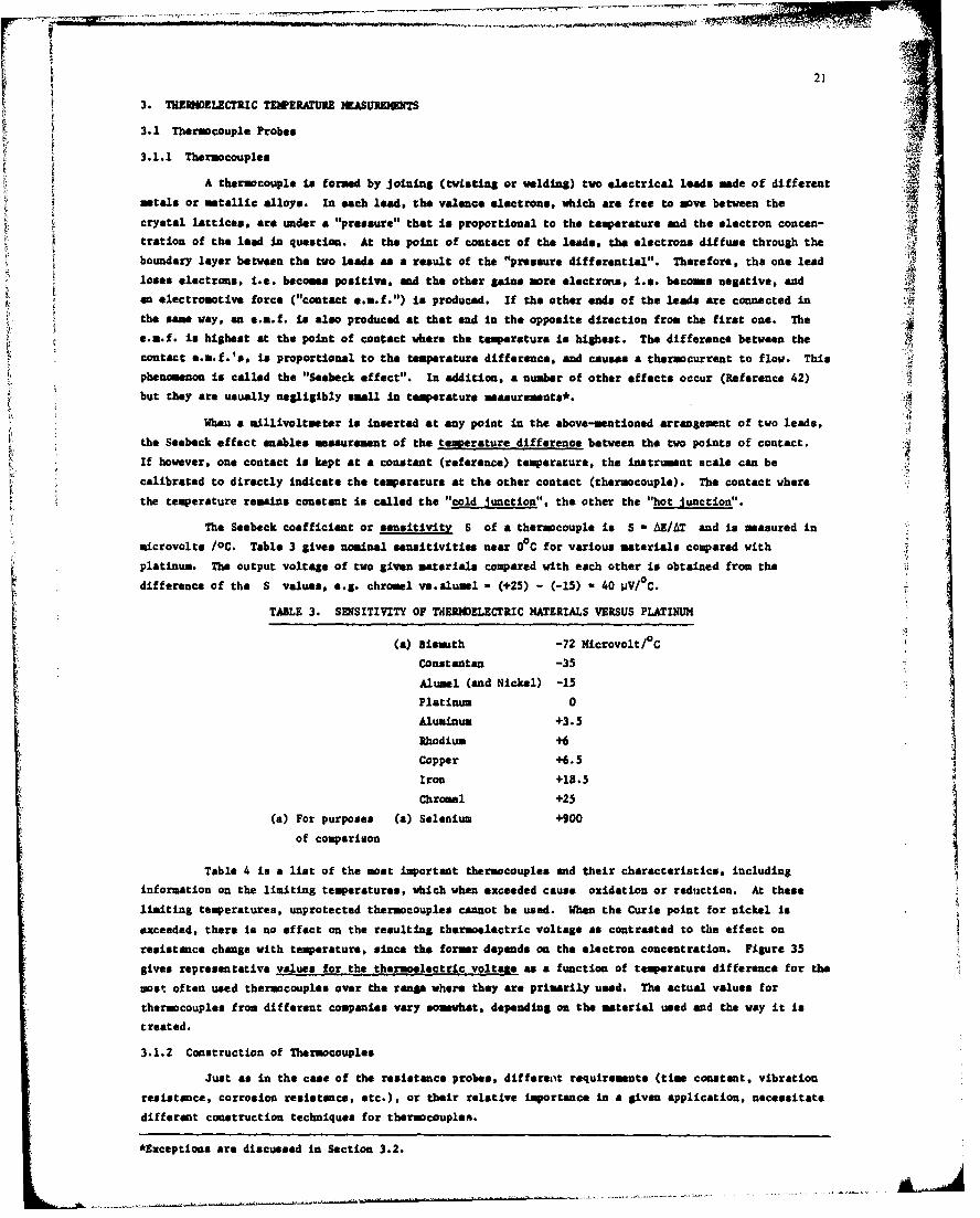
S3. THSIE ELECTIIC TEWIERATURE WASURja2 2

3.1 Thermocouple Probes

3.1.1 Thermocouples 4,

A thermocouple is formed by joining (twisting or welding) two electrical leads made of different

metals Or metallic alloys. In each lead, the valence electrons, which are free to move between the

crystal lattices, are under a "pressure" that is proportional to the temperature and the electron concean-

tration of the lead in question. At the point of contact of the leads, the electrons diffuse through the

boundary layer between the two leads as a result of the "pressure differential". Therefore, the one lead

loses electrons, i.e. becomes positive, and the other gains more electrons, i.e. becomes negative, and

an electromotive force ("contact e.m.f.") is produced. If the other ends of the leads are connected in

the same way, an o.a.f, is also produced at that end in the opposite direction from the first one. The

e.z.f. is highest at the point of contact where the temperature is highest. The difference between the

contact o.af.s', is proportional to the temperature difference, and causes a thermocurrent to flow. This

phenomenon is called the "Seebeck effect". In addition, a number of other effects occur (Reference 42)

but they are usually negligibly small in temperature measurements*.

When a millivoltooter Is inserted at any point in the above-mentioned arrangement of two leads,

the Seebeck effect enables measurement of the temperature difference between the two points of contact.

If however, one contact is kept at a constant (reference) temperature, the instrument scale can be

calibrated to directly indicate the temperature at the other contact (thermocouple). The contact where

the temperature remains constant is called the "cold Junction". the other the "hot Junction'.

The Seebeck coefficient or sensitivity S of a thermocouple is S = AE/AT and is measured in

microvolts /OC. Table 3 gives nominal sensitivities near OC for various materials compared with

platinum. The output voltage of two given materials compared with each other is obtained from the

difference of the S values. e.g. chromel vw.alumsl - (+25) - (-15) - 40 pV/°C.

TABLE 3. SENSITIVITY OF TdE.RWELECTRIC MATERIALS VERSUS PLATINUM

(a) Bismuth -72 Microvolt/°C

Constantan -35

Alumel (and Nickel) -15

Platinum 0

Aluninum +3 -5

Rhodium +6

Copper +6.5

Iron +18.5

Chromel +25

(a) For purposes (a) Selenium +900

of comparison

Table 4 is a list of the most important thermocouples and their characteristics, including

information on the limiting temperatures, which when exceeded cause oxidation or reduction. At these

limiting temperatures, unprotected thermocouples cannot be used. When the Curie point for nickel is

exceeded, there is no effect on the resulting thermoelectric voltage as contrasted to the effect on

resistance change with temperature, since the former depends on the electron concentration. Figure 35

gives representative values for the thermoelectric voltage as a function of temperature difference for the

most often used thermocouples over the range where they are primarily used. The actual values for

thermocouples from different companies vary somewhat, depending on the material used and the way it is

treated.

3.1.2 Construction of Thermocouples

Just as in the case of the resistance probes, differenct requirements (time constant, vibration

resistance, corrosion resistance, etc.), or their relative importance in a $iven application, necessitate

different construction techniques for thermocouples.

*Exceptione are discussed in Section 3.2.

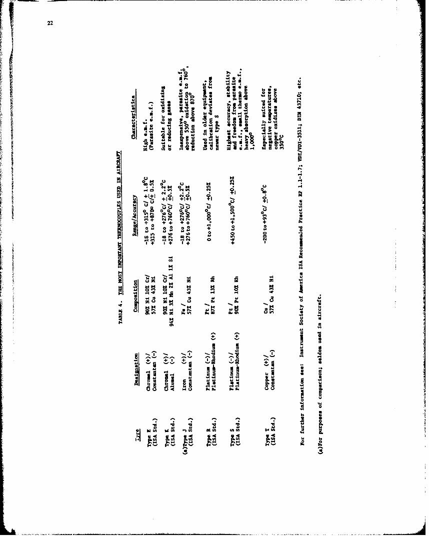
1 22

.40

000

104 9. .84 N . 1

41 0

VU41 V U .

A0I wR u. m. 8

w u 1 3mW 0fl4 1 sU

SO 01 OUIi

0 s 0 + + 0+

.- 0 .U0 f 0 03*

0010 0 0 UIIN %0D 0

T I +

4f 44 Mbe- C-4 N U

4 4 r4 %W .- IA

44

z 44"H 1, 4

m4 mN4c 6mL

144 14

0 H

-44 -4

41N UNUS f 1

N17 PI 0 P4 U'I41

41 Is

H 1-4 1.-4

_ _ _ 23

ismd fFigures 36& through d show."open elements (exposed hot junctions). The first one (Figure 36a)

tomd fa single lead thermocoauial cable; the center conductor in constantan wire and the outer A

conductor is copper tubing. More typically two insulated wires are used, sand they are joined at the

t hot junction by twistini; or better yet, by welding or silver soldering. When measurements must be madein a medium that is moiving at high speeds, or if the element mus~t be mechanically protected, an open

element with a Protective shield (Figure 36g) is used. In all the previously mentioned types, the indium

to be measured is in direct contact with the thermocouple so that as a result of the small mass, very

small time constants are obtained.

For use in media at high pressures, or if the medium is corrosive or an electrical conductor,

the thermocouples must be housed iu sealed tubes (Figures 36o and f). In these well-type elements,

the wires are often welded to the tube and hence grounded at the contact point (Figure 36e). ThisA

normally excludes any arrangement of several elements in parallel (for indication of mean temperatureN-with a single instrument),* but yields smeller time constants then the well-type elements with an

ungrounded junction shown in Figure 36f. Examples of another type of open element, the so-called foil

thermocouples that are used for surface temperature measurements, are shown in Figure 37. They are madeof flat ribbons, and are provided with temporary carriers of polyamide film. These elements are directly

attached to the surface with a ceramic cement and are sometimes sprayed with a protective ceramic

coating.

3.1.3 Construction of Probes with Thermocouples

If a thermoelement is equipped with a threaded or bayonet fitting, some other type of fitting,

or even a housing, the arrangement is usually called a thermocouple probe. In contrast to the

resistance probes which are usually provided with an electrical connector, the thermocouple probes have

lead wires without terminals, eyes or even connectors with pins made of the same material as the element.

Depending on the purpose for which they are used, there are numerous types of probe

construction, so that only examples of the most important types can be given hare. Probes for measurements

in liquids and gases are usually cylindrical in shape (Figure 38a), and the threaded fitting is often

manufactured with a clamp so that the limmrsion depth of the element can be adjusted (Figure 38b). The

element itself may be open, equipped with a shield (Figure 38a) or cloaled (Figure 38c). Figure 38d Ashows an open model with two separate thermocouples, one of which can be used for individual measurements,

and the other for obtaining average temperature values when connected with other elements.

For measurements ina a rapidly moving gas stream, the gas temperature probes (TAT~ or stagnation

probes) shown in Figures 39 and 40 are used. They are always open elements and the housing usually has

large intake openings, but small exhaust openings, so that the entering gas stream is adiabaticallycompressed. Figures 39a sand 39b show simple models; Figure 39c, however, shows a model that is bettersuited for measurements in high speed gases, e.g. exhaust gas temperatures. In order to measure the

__________________0_

outside air temperature in supersonic aircraft, where stagnation temperatures can be +150 C or higher,special types must be used. Figure 40 shows a mouU± with two concentric radiation shields in the housingwhich significantly reduces the otherwise relatively large radiation error.

Finally, Figure 41 shows various probes for measuring temperature in solid bodies and on surfaces.

The one in Figure 4la~is a special spring-loaded model for measuring the temperature of the cylinder head

of an aircraft engine. The spring presses the enclosed probe element against the bottom of a bored hole

in the cylinder head. Figure 41b shows a semi-open probe with a threaded fitting designed to measure the

temperature of brake drums. Figure 41f shows a clamp type probe which can be mounted on a pipeline. The

gasket probes shown in Figure 41c and d are mounted like gaskets under spark plugs or screws. Figure 4le

gives a front and side view of a probe that is riveted into a hole in the surface whose temperature

is to be measured.

At this point, it must be mentioned that there are a number cf other special types of probes,

e.g. those that are more applicable for directly measuring the heat flux from and to surfaces, rather

than for temperature measurements (see References 91 through 94).

24

3.*2 Connecting Wires and Extenbion Leads

In Figure 42a, two leads z and y made of different materials are shown, which are connectedto each other at points P~ and P2 by welding, twisting, aet. When P1 and P are at different

temperatures (T 1 and T 2), a current is genarated that is proportional to the temperature difference.

The direction of the current depends on whether T1 is greater or less than T. A temperature difference,

therefore, produces an electromotive force (thermal a.a.f.), if this temperature difference occurs be-

tween two points of contact of different metals. Temperature gradients anywhere within lead x or lead

y will have no effect if each is made of a homogeneous material*.

In thermocouple circuits, symmtrical connection points (or even lines) of a differ&Lt

material can be arranged differentially without consequence as long ar these points (or the connection

points of the lines) are at the same temperature (i~e., as long as the voltages that are generated atthe points where the two different materials are connected are cancelled). Hence, if one of the

conductors shown in Figure 42a Is brokaai and a millivoltmeter inserted (Figure 42b) with leads made of

material z (e.g., copper) and both points of contact (P3 and P4 of the broken lead are kept at the

same temperature, there is no effect on the thermal e.m.f., although two new - but differentially

arranged - thermocouples P3 and P4 have been formed. Their common temperature T3 can be different

from T1 and T2 and even from the temperature at the instrument, since in the letter case the tempera-

ture gradients appear in similar leads (both of material z). If however, points P 3 and P 4 were. atV different temperatures, their thermoelectric voltages would no longer cancel out and the resulting

thermoelectric voltage of the circuit would be equal to the algebraic sum of all the individual voltages.

This is equally true for a point P5, which per se must have a single temperature, and it can also be

considered a differential connection, y'/P5 to P /y. This circuit (Figure 42b) is useful for measuring

temperature differences or rate of temperature changes** (cf. sect. 2.2.3.2).

Usually, it is desirable to directly measure the temperature T at point Pi, in which case

the circuit shown in Figure 42c is better for several reasons.* Instead of opening one lead and usingtwo thermocouples, point P 2 is opened and the instrument is connected to points P 2 and P 3 . Again,

two new differentially arranged thermocouples have been formed, and their temperature must be equal. If

this temperature T 2 is kept at 0 C as a reference temperature, using for example a container with

melting ice, then the temperature difference AT between T1 and T2 would equal T1 in 0 C. If

on the other hand, a thermostat is used to keep T 2 at +40 0C, then AT - T1 400 * The indicator

scale must then be shifted by +400 C so that instead of the temperature difference, the temperature

T1- AT + 40 0C is directly indicated. In aircraft, another type of reference point formation is often

used (see below).

When the leads of the thermocouples are short and relatively high temperatures are to be

measured, e.g. temperatures in an engine, it would be difficult to maintain a constant temperature at the

Junctions P 2 and P 3 because of the large fluctuating temperature gradients between the engine and

the indicator. In this case, points P 2 and P 3 have to be moved, using so-called extension leads,

to a more favorable position with points P 1 2 and P 1 3 as reference points (Figure 43). The extension

leads xf and y' must, however, be made of the esae material as x and y, otherwise additional

thermoelectric voltages are generated. In other words, Chromel-Alumel thermocouples are lengthened

with Chromel-Alumel leads. The tie lugs at P2 and P3 can be made of any material v and can be *

at any temperature with respect to T 1 and T 3 (and also with respect to each other). It is essential,however, that the junctions x/w and w/x', as well as y/w and w/y', are at the same temperature, so

that there are no parasitic thermoelectric currents. This condition does not always hold true in plug

type connectors or in junction boxes, and it is advisable to use special inserts of thermoelectric

material, or a parallel arrangement of the input and output leads for approximately 10 cm and thentwisting them so that they will be close to the same temperature.

*Cf. below the effect of heterogeneous leads.

**Non-linear thermocouple output voltages sust be taken into account.

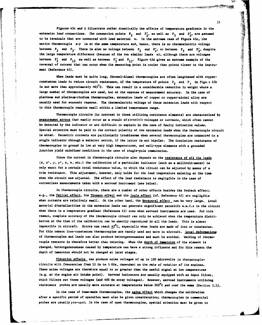
Figures 43c and d illustrate rather drastically the effects of temperature gradients in theextension lead connections. The connection points P2 and P, as well as P3 and P , are assumed

to be terminals that are connected with lead material w. In the extreme case of Figure 43c, the =4

entire thermocouple x-y is at the same temperature and, hence, there is no thermoelectric voltage

between P2 and P3 . There is also no voltage between P2 and P•, or between P3 and Pj, despite

the large temperature difference (because of the two similar leads w), although there are voltagesbetween P' and P1 as well as between P' and P Figure 43d gives an extreme example of the

reversal of current that can occur when the measuring point is cooler than points closer to the instru-

ment (Reference 43). A

When leads must be quite long, Chromel-Alumel thermocouples are often lengthened with copper-

Sconstantan leads to reduce circuit resistance, if the temperature of points P2 and P3 in Figu. 43b

is not more than approximately +650C. This can result in a considerable reduction in weight where a

large number of thermocouples are used, but at the expense of measurement accuracy. In the case of

platinum and platinum-rhodium thermocouples, extension leads of copper or copper-nickel alloy are

usually used for economic reasons. The thermoelectric voltage of these extension leads with respect

to this thermocouple remains small within a limited temperature range.

Thermocouple circuits (in contrast to those utilizing resistance elements) are characterized by

measurement errors that easily occur as a result of parasitic voltages or currents, which often cannot

be detected by the indicator or are difficult to explain in the case of faulty indication values.Special attention must be paid to the correct polarity of the extension leads when the thermocouple circuit

is wired. Parasitic currents are particularly troublesome when several thermocouples are connected to a

single indicator through a selector switch, if the latter is not bipolar. The insulation resistance of

thermocouples to ground is low at very high temperatures, and well-type elements with a grounded

junction yield undefined conditions in the case of single-pole commutation.

Since the current in thermocouple circuits also depends on the resistance of all the leads

(x, x', y, y', z, w, etc.) the calibration of a particular indicator (such as a millivolt-meter) isonly exact for a certain total resistance value, to which the circuit can be adjusted by means of a

trim resistance. This adjustment, however, only holds for the lead temperature existing at the time

when the circuit was adjusted. The effect of the lead resistance is negligible in the case of

currentless measurements taken with a servoed instrument (see below).

In thermocouple circuits, there are a number of other effects besides the Seebeck effect;

e.g., the Peltier effect, the Thomson effect and the Joule effect (cf. Reference 42) are negligible

when currents are relatively small. On the other hand, the Becguerel effect can be very large. Local

material dissimilarities in the extension leads can generate significant parasitic e.m.f.s in the circuit

when there is a temperature gradient (Reference 42) even when servoed instruments are used. For this

reason, complete accuracy of the thermocouple circuit can only be achieved when the temperature distri-

bution at the time of the calibration can be exactly reproduced in all the leads. This is almost

impossible in aircraft. Errors can reach +2 °C, especially when leads are made of iron or constantan.

For this reason iron-constantan thermocouples are rarely used any more in aircraft. Local deformations

of thermocouples and leads can also produce heterogeneousness and must be avoided. Welding of thermo-

couple contacts is therefore better than twisting. When the depth of imersion of the element is

changed, heterogeneousness caused by temperature can have a strong influence And for this reason the

depth of immersion should not be changed at later stages.

Vibration effects can produce noise voltages of up to 100 microvolts in thermocouple-

circuits with frenuencies from 10 Hs to 5 KRs, dependent on the rate of rotation of the engines.

These noise voltages are therefore equal to or greater than the useful signal at low temperatures

(e.g. at the engine air intake point). Servoed indicators are usually equipped with an input filter,

which filters out these voltages (and 400 Hz stray voltages). However, servoed instruments utilizing

resistance probes are usually more accurate at temperatures below 200 0 C and cost the same (Section 5.3).

In the case of home-made thermocouples, the asing effect which changes the calibration

after a specific period of operation must also be given consideration; thermocouples in commercial

probes are usually pre-aged. In the case of open thermocouples, special attention must be given to

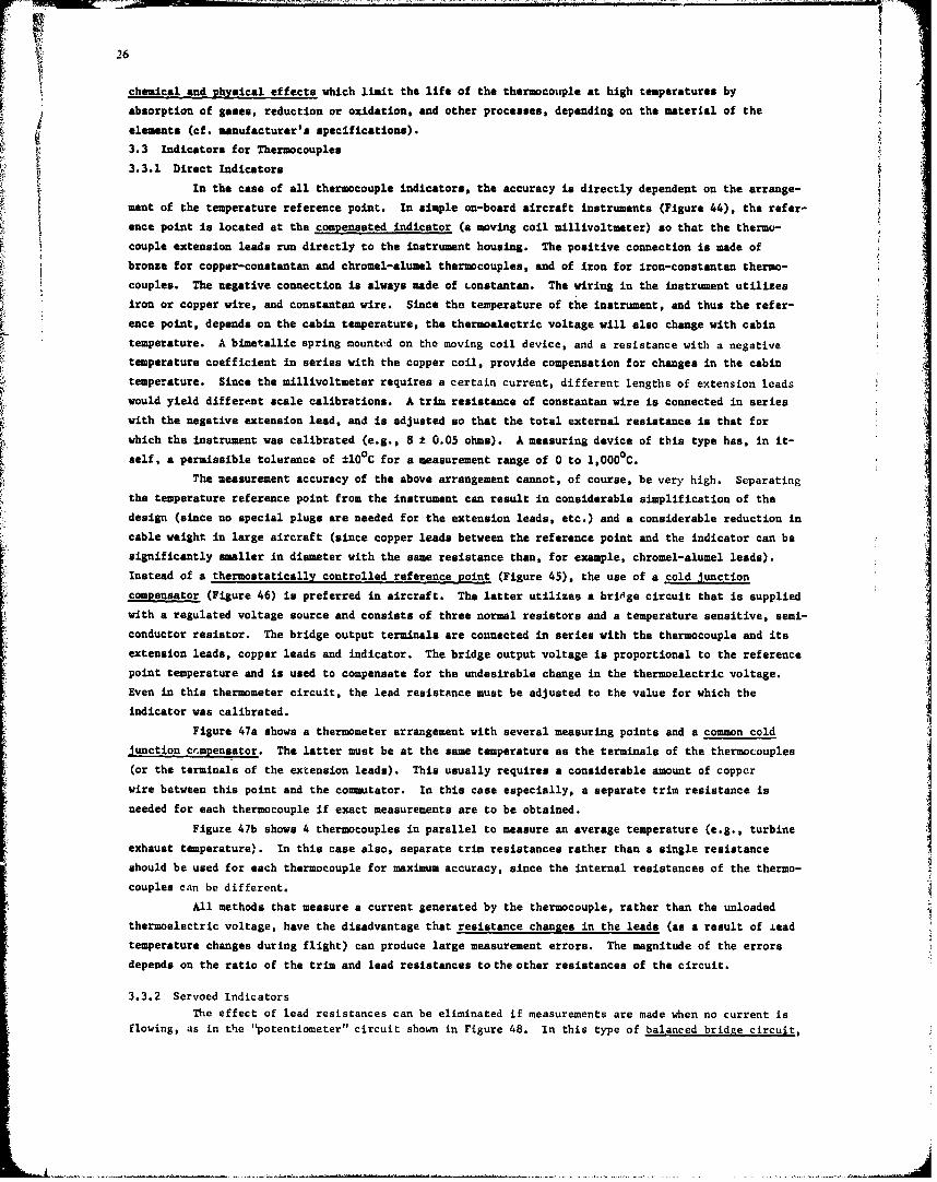
26

chemical and physical effects which limit the life of the thermocouple at high temperatures by

absorption of gases, reduction or oxidation, and other processes, depending on the material of the

elements (cf. manufacturer's specifications).

3.3 Indicators for Thermocouples

3.3.1 Direct Indicators

In the case of all thermocouple indicators, the accuracy is directly dependent on the arrange-

ment of the temperature reference point. In simple on-board aircraft instruments (Figure 44), the refer-

ence point is located at the compensated indicator (a moving coil millivoltmeter) so that the thermo-

couple extension leads run directly to the instrument housing. The positive connection is made of

bronze for copper-constantan and chromel-alumel thermocouples, and of iron for iron-constantan thermo-

couples. The negative connection is always made of constantan. The wiring in the instrument utilizes

iron or copper wire, and constantan wire. Since the temperature of the instrument, and thus the refer-

ence point, depends on the cabin temperature, the thermoelectric voltage will also change with cabin

temperature. A bimetallic spring mounted on the moving coil device, and a resistance with a negative

temperature coefficient in series with the copper coil, provide compensation for changes in the cabin

temperature. Since the millivoltmeter requires a certain current, different lengths of extension leads

would yield different scale calibrations. A trim resistance of constantan wire is connected in series

with the negative extension lead, and is adjusted so that the total external resistance is that for

which the instrument was calibrated (e.g., 8 ± 0.05 ohms). A measuring device of this type has, in it-

self, a permissible tolerance of i10°C for a measurement range of 0 to 1,000°C.

P The measurement accuracy of the above arrangement cannot, of course, be very high. Separating

the temperature reference point from the instrument can result in considerable simplification of the

design (since no special plugs are needed for the extension leads, etc.) and a considerable reduction in

cable weight in large aircraft (since copper leads between the reference point and the indicator can be

significantly smaller in diameter with the same resistance than, for example, chromel-alumel leads).

Instead of a thermostatically controlled reference point (Figure 45), the use of a cold junction

compensator (Figure 46) is preferred in aircraft. The latter utilizes a brit•ge circuit that is supplied

with a regulated voltage source and consists of three normal resistors and a temperature sensitive, semi-

conductor resistor. The bridge output terminals are connected in series with the thermocouple and its

extension leads, copper leads and indicator. The bridge output voltage is proportional to the reference

point temperature and is used to compensate for the undesirable change in the thermoelectric voltage.

Even in this thermometer circuit, the lead resistance must be adjusted to the value for which the

indicator was calibrated.

Figure 47a shows a thermometer arrangement with several measuring points and a common cold

junction cmpensator. The latter must be at the same temperature as the terminals of the thermocouples(or the terminals of the extension leads). This usually requires a considerable amount of copperwire between this point and the commutator. In this case especially, a separate trim resistance is

needed for each thermocouple if exact measurements are to be obtained.

Figure 47b shows 4 thermocouples in parallel to measure an average temperature (e.g., turbine

exhaust temperature). In this case also, separate trim resistances rather than a single resistance

should be used for each thermocouple for maximum accuracy, since the internal resistances of the thermo-

couples can be different.

All methods that measure a current generated by the thermocouple, rather than the unloaded

thermoelectric voltage, have the disadvantage that resistance changes in the leads (as a result of ieadtemperature changes during flight) can produce large measurement errors. The magnitude of the errors

depends on the ratio of the trim and lead resistances to the other resistances of the circuit.

3.3.2 Servoed IndicatorsThe effect of lead resistances can be eliminated if measurements are made when no current is

flowing, as in the "potentiometer" circuit shown in Figure 48. In this type of balanced bridge circuit,

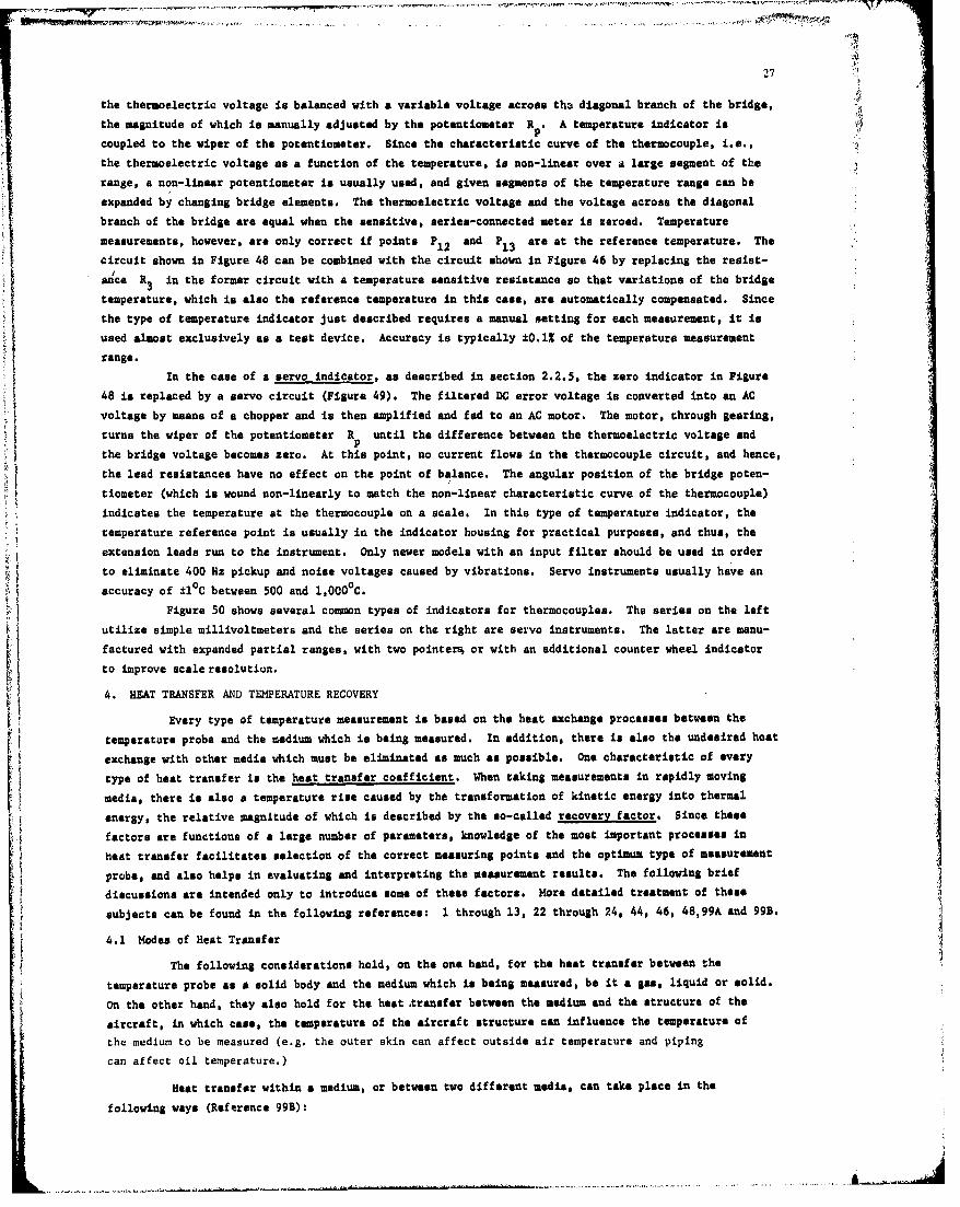
27

the thermoelectric voltage is balanced with a variable voltage across tho diagonal branch of the bridge,

* the magnitude of which is manually adjusted by the potentiometer R *A temperature indicator is

coupled to the wiper of the potentiometer. Since the characteristic curve of the thermocouple, i.e.,the thermoelectric voltage as a function of the temperature, is non-linear over a large segment of the

range, a non-linear potentiometer is usually used, and given segments of the temperature range can be

* expanded by changing bridge elements. The thermoelectric voltage and the voltage across the diagonal

branch of the bridge are equal when the sensitive, series-connected meter is zeroed. Temperature

measurements, however, are only correct if points P 2 and P 3 are at the reference temperature. The

circuit shown in Figure 48 can be combined with the circuit shown in Figure 46 by replacing the resist-

ance R3 in the former circuit with a temperature sensitive resistance so that variations of the bridge

tempratrewhich is also the reference temperature in this case, are automatically compensated. Since

themtpraue o temperature indicator just described requires a manual setting for each measurement, it is%

used almost exclusively as a test device. Accuracy is typically ±0.12 of the temperature measurement

range.

in the case of a servo indicator, as described in section 2.2.5, the zero indicator in Figure

48 is replaced by a servo circuit (Figure 49). The filtered DC error voltage is converted into an AC

voltage by means of a chopper and is then amplified and fed to an AC motor. The motor, through gearing,

turns the wiper of the potentiometer R until the difference between the thermoelectric voltage andp

the bridge voltage becomes zero. At this point, no current flows in the thermocouple circuit, and hence,

the lead resistances have no effect on the point of balance. The angular position of the bridge poten-

tiometer (which is wound non-linearly to match the non-linear characteristic curve of the thermocouple)

indicates the temperature at the thermocouple on a scale. In this type of temperature indicator, the

temperature reference point is usually in the indicator housing for practical purposes, and thus, the

extension leads run to the instrument. Only newer models with an input filter should be used in order

to eliminate 400 Hz pickup and noise voltages caused by vibrations. Servo instruments usually have an

accuracy of ±1 C between 500 and 1,000 C.

Figure 50 shows several common types of indicators for thermocouples. The series on the left

utilize simple millivoltmeters and the series on the right are servo instruments. The latter are menu-

factured with expanded partial ranges, with two pointerM or with an additional counter wheel indicator

to improve scale resolution.

4. HEAT TRAN4SFER AND TEMPERATURE RECOVERY

Every type of temperature measurement is based on the heat exchange processes between the

temperature probe and the medium which is being measured. In addition, there is also the undesired hoat

exchange with other media which must be eliminated as much as possible. One characteristic of every

type of heat transfer is the heat transfer coefficient. When taking measurements in rapidly moving

media, there is also a temperature rise caused by the transformation of kinetic energy into thermal

energy, the relative magnitude of which is described by the so-called recovery factor. Since these

factors are functions of a large number of parameters, knowledge of the most important processes in

heat transfer facilitates selection of the correct measuring points and the optimum type of measurement

probe, and also helps in evaluating and interpreting the measurement results, The following brief

discussions are intended only to introduce some of these factors, More detailed treatment of these

subjects can be found in the following references: I through 13, 22 through 24, 44, 46, 48,99A and 99B.

4.1 Modes of Heat Transfer

The following considerations hold, on the one hand, for the heat transfer between the

temperature probe as a solid body and the medium which is being measured, be it a gas, liquid or solid.

On the other hand, they also hold for the heat transfer between the medium and the structure of the

aircraft, in which case, the temperature of the aircraft structure can influence the temperature of

the medium to be measured (e.g. the outer skin can affect outside air temperature and piping

can affect oil temperature.)

Heat transfer within a medium, or between two different media, can take place in the

following ways (Reference 993):

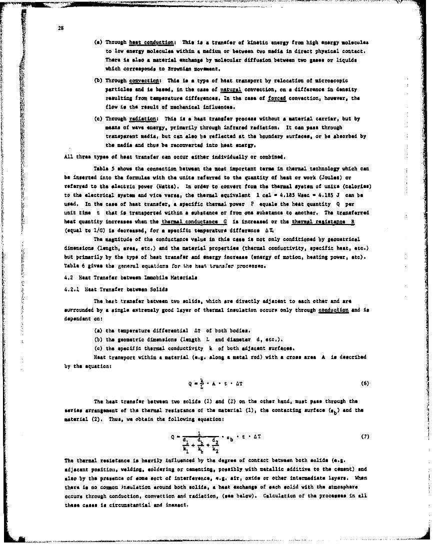
(a) Through heat conduction: This to a transfer of kinetic energy from high energy moleculesto low energy molecules within a medium or between two media in direct physical contact.Id There Is also a material e@chang* by molecular diffusion between two gases or liquidswhich corresponds to Brownian movement.

(b) Through convection: This is a type of heat transport by relocation of microscopicparticles and is based, in the cooe of natural convection, on a difference in densityresulting from temperature differences. In the case of foce convection, however, theflow is the result of mechanical influences.

(c) Through radiaions This is a heat transfer process without a material carrier, but bymeans of wave energy, primarily through infrared radiation. It can pass throughtransparent media, but can also be reflected at the boundary surfaces, or be absorbed by .

the media and thus be reconverted into heat energy.

All three types of heat transfer can occur either individually or combined.

Tabl 5 sowsthe connection between the most important terms In thermal technology which can0,; be inserted into the formulae with the unite referred to the quantity of heat or work (Joules) or

referred to the electric power (Watts). In order to convert from the thermal system of units (calories)to the electrical system and vice versa, the thermal equivalent 1 cal a 4.185 Wesc a 4.185 J can be

14 used. In the case of heat transfer, a specific thermal power P equals the heat quantity Q perunit tine t that is transported within a substance or from one substance to another, The transferredheat quantity increases when the thermal conductance G is Increased or the thermal resistance R(equal to 1/G) is decreased, for a specific temperature difference AT.

The magnitude of the conductance value in this case Is not only conditioned by geometricaldimensions (length, area, etc.) and the material properties (thermal conductivity, specific heat, etc.)but primarily by the type of heat transfer and energy increase (energy of motion, heating power, etc).Table 6 gives the general equations for the heat transfer processes#

Tranfer etwen Slid

4.2 Heat Transfer between Immobile Materials

The hest transfer between two solids, which are directly adjacent to each other and aresuruddby a single extremely good layer of thermal insulation occurs only through conduction and is

dpneton:

(a) the temperature differential AT of both bodies.

Mb the geometric dimensions (length L and diameter d, etc.),

(c) the specific thermal conductivity k of both adjacent surfaces.Heat transport within a material (e.g. along a metal rod) with a cross area A is described

by the equation:

Q A * t * AT (6)

The heat transfer between two solids (3.) and (2) on the other hand, must pass through theseries arrangement of the thermal resistance of the material (1), the contacting surface (0b and the

material (2). Thus, we obtain the following equation:

Q* AT (7)

k, kbk2

The thermal resistance is heavily Influenced by the degree of contact between both solids (e.g.

adjacent positiou, welding, soldering or cementing, possibly with metallic additive to the cement) and

also by the presence of some sort of interference, a.g. air, oxide or other intermediate layers. When

there is no common insulotion around both solids, a heat exchange of each solid with the atmosphereoccurs through conduction, convection and radiation, (see below). Calculation of the processes in all

these cases is circumstantial and inexact.

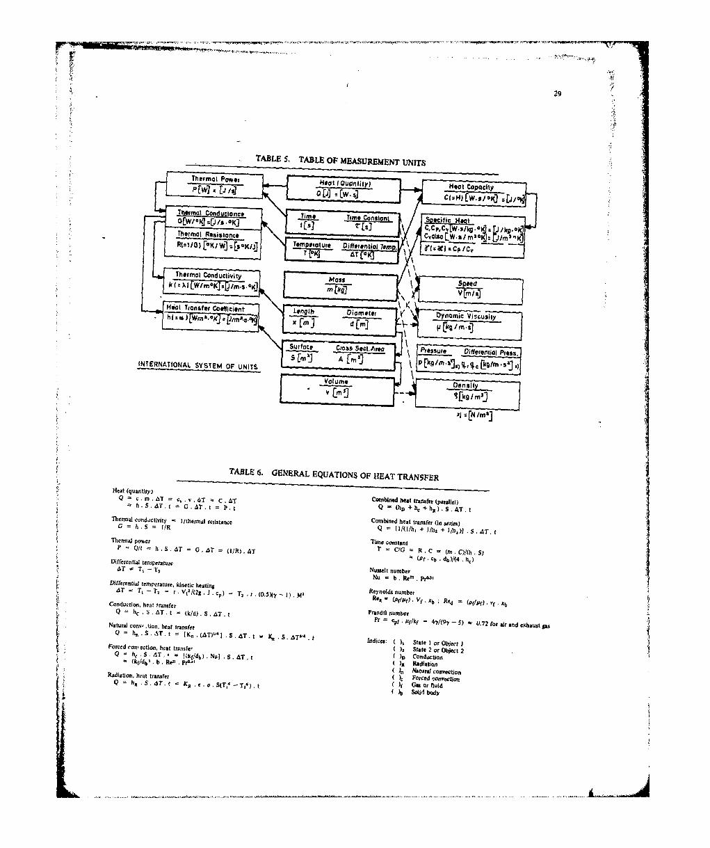
29

TABLE 5. TABLE OF MEASUREMENT UNITS

/ABL 6. GENRA EQUATION OOHAXTAS

C o m i n e h e a t t r a n s f eru r ( inf x ie

Thermal Codutwer Ms

Hstritilm erat Tanfr Cefceten~ Di umete numberAT T 1 -1- Nu fm ]. d[m p AiI

DifferenSurfal tem eraure kinel hatinAT~ ~~~~~ ~ ~ ~~~~~~ T1 n -T4.3

2( 1 ~ ~ 2 * .( S 7 ) 2

R y o d n m e

Natural co--Lens!( tafe

Hore dt (q u n eti on ety t a se)( o n u t oQ C. In.S.AT, c' r b. Nul& C.SAT t ( )b Radiat tr nsfr(aall(kr/dbl. b.T~ =e P., Q (11 +n hera coh nec- T.tio

Radieati on, itvt h terlrsstneCm ie eat transfe I- Gi r (lid eisG0 h5 - S 1 +.11O1S(+T5 /3T2 4S.

AT.Ileilpwr iecntn

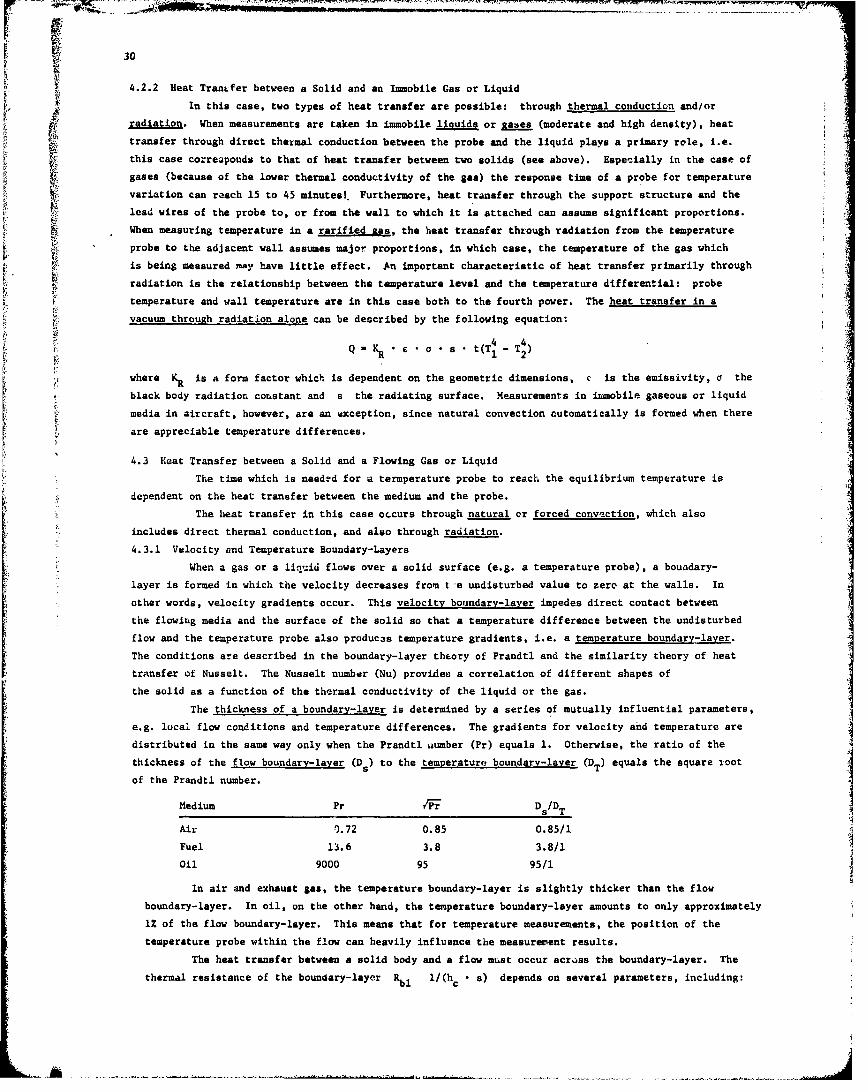
r 4.2.2 Heat TranLfer between a Solid and an Immobile Gas or Liquid

In this case, two types of heat transfer are possible: through thermal conduction and/or 4

radiation. When measurements are taken in immobile liquids or ases (moderate and high density), heat

transfer through direct thermal conduction between the probe and the liquid plays a primary role, i.e.

this case correapouds to that of heat transfer between two solids (see above). Espeeially in the case ofgases (because of the lower thermal conductivity of the gas) the response time of a probe for temperature

variation can reach 15 to 45 minutest. Furthermore, heat transfer through the support structure and the

lead wires of the probe to, or from the wall to which it is attached can assume significant proportions.

When measuring temperature in a rarifLed gas, the heat transfer through radiation from the temperature

probe to the adjacent wall assumes major proportions, in which case, the temperature of the gas which,k is being measured may have little effect. An important characteristic of heat transfer primarily through

radiation is the relationship between the temperature level and the temperature differential: probetemperature and wall temperature are in this case both to the fourth power. The heat transfer in a

vacuum through radiation alone can be described by the following equation:

4 4Q*KR C a * t(T1 T)

where KR is a form factor which is dependent on the geometric dimensions, c is the emissivity, a the

black body radiation constant and s the radiating surface. Measurements in iLmobile gaseous or liquid

media in aircraft, however, are an exception, since natural convection automatically is formed when there

are appreciable temperature differences.

4.3 Heat Transfer between a Solid and a Flowing Gas or Liquid

L The time which is needrd for a temperature probe to reach the equilibrium temperature is

dependent on the heat transfer between the medium and the probe.

The heat transfer in this case occurs through natural or forced convection, which also

includes direct thermal conduction, and also through radiation.

4.3.1 Velocity and Temperature Boundary-Layers

When a gas or a liquid flows over a solid surface (e.g. a temperature probe), a boundary-

layer is formed in which the velocity decreases from t e undisturbed value to zero at the walls. In

other words, velocity gradients occur. This velocity boundary-layer impedes direct contact between

the flowing media and the surface of the solid so that a temperature difference between the undisturbed

flow and the temperature probe also produczs temperature gradients, i.e. a temperature boundary-layer.

The conditions are described in the boundary-layer theory of Prandtl and the similarity theory of heat

trAnsfer of Nusselt. The Nusselt number (Nu) provides a correlation of different shapes of

the solid as a function of the thermal conductivity of the liquid or the gas.

The thickness of a boundary-layer is determined by a series of mutually influential parameters,e.g. local flow conditions and temperature differences. The gradients for velocity and temperature are

distributed in the same way only when the Prandtl aumber (Pr) equals 1. Otherwise, the ratio of the

thickness of the flow boundary-layer (Ds) to the temperature boundary-layer (D equals the square toot

of the Prandtl number.

Medium Pr p-r Ds/DT

Air ).72 0.85 0.85/1

Fuel 13.6 3.8 3.8/1

Oil 9000 95 95/1

In air and exhaust gas, the temperature boundary-layer is slightly thicker than the flow

boundary-layer. In oil, on the other hand, the temperature boundary-layer amounts to only approximately

1% of the flow boundary-layer. This means that for temperature measurements, the position of the

temperature probe within the flow can heavily influence the measurement results.

The heat transfer between a solid body and a flow must occur across the boundary-layer. The

thermal resistance of the boundary-layer Rbl /(hc s) depends on several parameters, including:

31

(a) the geometric dimensions of the body in the flow,

(b) the thermal conductivity of the flowing media,

(c) the Reynolds number or the type of flow (laminar or turbulent),(d) the Prandtl number,

(e) the temperatures of the body and the flowing media,(f) the type of convection (natural or forced),

(g) pressure (in the case of a gas),(h) Mach number

4.3.2 Heat Transfer by Natural Convection

In the case of natural convection, a flow is generated in an originally imobile liquid (or

gas) at a solid (wall or temperature probe) when there is a temperature difference between both (e.g.

self-heating of the probe). This process occurs very slowly, depends on the magnitude of the temperature

differential, and seldom reaches a steady-state condition. The direction and rate of the flow and the

thickness of the boundary layer are influenced by the configuration of the surrounding walls, their

insulation and a number of other factors which are very difficult to determine.

The dependence on the given temperature difference AT between the solid and the gas or

liquid is characteristic of natural convection. The heat exchange occurs primarily by conduction since

the velocity of the gas or the liquid can only reach relatively small values and the flow around a

temperature probe can be considered laninar.

The heat transfer coefficient for natural convection is:

h n- K a (AT) 1/4 (9)

where K nis a constant that is a function of the heat transfer value, velocity distribution,

geometric conditions, etc. The heat transfer is:

On K.a (AT)~' t (10)

Temperature measurements with natural convection (e.g. conpressor intake or exhaust temperature

measurement on an engine which has just been cut) are very rare and are only meaningful if temperature

probes with very small tine constants are used together with a measuring technique where the self-

heating of the probe is negligibly small. For further details about natural convection, the book of

McAdams (Reference 12) can be used, which describes the influence of shape, etc.

4.3.3 Heat Transfer by Forced Convection

In the great majority of all temperature measurements in aircraft, heat transfer occurs byIforced convection, in which case, the motion of the medium which is being measured is caused by the

speed of the aircraft, the engine, a fuel pump, etc. The type of flow can be either laminar or

* turbulent, or separated from the body, depending on the given conditions. The velocity of the flowtsometimes reaches such values that there is a considerable temperature rise when it impacts on a solid,

* and other effects must also be taken into account, e.g. the effect of compressibility in the case of gas.

4.3.3.1 Heat Transfer in a Subsonic Flow

In laminar flow, all of the flowing particles move longitudinally. The heat transfer in this

case (within certain limits) is almost independent of the Reynolds number Re, the total pressure PTand the Mach number M, and occurs almost completely by thermal conduction. When the rate of flow

increasos, i.e. when the Reynolds number becomes greater, there is an irregular lateral motion of the

flowing particles in addition to the longitudinal motion, so that the adjacent flow layers are mixed.

In this type of turbulent flow, the lines of flow only represent the average values of the paths of the

flow particles. The transition from one type of flow to the other takes place sharply at a specific

rte of flow (critical Reynolds number), but can be influenced by a number of different factors

(Wernces99A and 99B). The local Reynolds number must be referred to as the distance x from the

forward edge or to the diameter d of the solid (Re, x or Re, d). As the Reynolds number

increases, i.e. as the velocity increases (or in gaseous flows when the temperature drops* and the

In liquids, when the temperature rises.

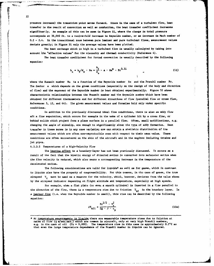
32

r pressure increase) the transition point moves forward. Since in the case of a turbulent flow, beat

transfer is the result of convection as wall as conduction.* the heat transfer coefficient increases

significan~tly. An example of this can be seen in Figure 51, where the change in total pressure

corresponds at 36,000 ft. to a twelve-fold increase in Reynolds number, or an increase in Mach number of

0.2 - 2.4. In the transitional zone between pure laminar and pure turbulent f lowe, measurement values

deviate greatly; in Figure 51 only the average values have been plotted.

The heat "xchange which is high in a turbulent flow is usually calculated by taking into

account ~the "effective values" for the viscosity and thermal conductivity (Reference 4).

The heat transfer coefficient for forced convection is usually described by the following

equation:

h - f r0.31 (1c kf/d5 .Nu ade5 P

where the Nusselt number Nu is a function of the Reynolds number Re and the Prandtl number Pr.

The factor a which depends on the given conditions (especially on the design of the body and direction

of flaw) and the exponent of the Reynolds number is best obtained experimentally. Figure 52 shows

characteristic relationships between the Nusselt number and the Reynolds number wihich have been

obtained for different thermometers and for different directions of flow (parallel flow or cross flow,

References 5, 12, and 44). The given measurement value3 and formulae hold only under specific

conditions.

In addition to the previously discussed ideal flow conditions, there is also an eddy flow

aft a flow separation, which occurs for example in the wake of a cylinder hit by a cross flow, or

behind solids which project from a plane surface in a parallel flaw. Often, small modifications, e.g.

changing the angle of sideslip, are enough to significantly alter the type of eddy formation. Heat

transfer in these zones is in any case variable; one can obtain a statistic distribution of the

measurenent values which are often non-reproducible even with respect to their mean value. These

conditions are often encountered on the skin of the aircraft and in the engines including intakes and

jet pipes.

4.3.3.2 Temperatures of a High-Velocity Flow

The heating effect in a boundary-layer has not been previously discussed. It occurs as a

result of the fact that the kinetic energy of directed motion is converted into molecular motion when

the flow velocity is reduced, which also means a corresponding increase in the temperature of the

decelerated medium.

The following considerations are valid for liquids* as well as for gases, which in contrast

to liquids also have the property of compressibility. For this reason, in tha case of gases, the true

airspeed Vt must be used as a measure for the velocity, which, however, deviates from the value shown

by the airspeed indicator depending on flight altitude and temperature, especially at high speeds.

For example, when a flat plate (or even a smooth cylinder) is inserted in a flaw parallel to

the direction of the flow, there is a temperature rise due to friction Tf in the boundary layer. In

a laminar flow (i.e. when the Reynolds number is small), this rise can be described by the following

equation:

1/2 2Pr .V

Tkfl 2g *J c~ la

*At temperature measurements in liouids there are measurable temperature rises due to friction atrates of flow (5 m/sec.max.) which are common in aircraft, only at very high Prandtl numbers,e.g. in the case of oil (Pr a 9,000). The temperature rise in this case is approximately O.2C sothat even the large temperature dependence of the Prandtl number in liquids can bc ignored.

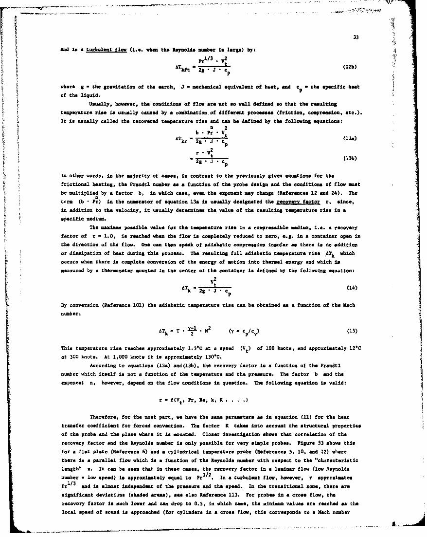
33

and in a turbulent flow (i.e. when the Reynolds number is large) by:

1/3 VPr&T a (12b)

kft 2S J * cp

where S - the gravitation of the earth, J a mechanical equivalent of heat, and c - the specific heatpof the liquid.

Usually, however, the conditions of flow are not so well defined so that the resulting

temperature rise is usually caused by a combination of different processes (friction, compression, etc.).

It is usually called the recovered temperature rise and can be defined by the following equations:n 2

b * Pr Vtkr 2 J • c (ha)P

2r ,2 ,t (13b)

P

In other words, in the majority of cases, in contrast to the previously given equations for the

frictional heating, the Prandtl number as a function of the probe design and the conditions of flow must

be multiplied by a factor b, in which case, even the exponent may change (References 12 and 24). Then

term (b • Pr) in the numerator of equation 13a is usually designated the recovery factor r, since,

in addition to the velocity, it usually determines the value of the resulting temperature rise in a

specific medium.

The maximum possible value for the temperature rise in a compressible medium, i.e. a recovery

factor of r - 1.0, is reached when the flow is completely reduced to zero, e.g. in a container open in

the direction of the flow. One can then speak of adiabatic compression insofar as there is no addition

or dissipation of heat during this process. The resulting full adiabatic temperature rise ATk which

occurs when there is complete conversion of the energy of motion into thermal energy and which is

measured by a thermometer mounted in the center of the container is defined by the following equation:

2VtAT V (14)

k 2Sg*J c

By conversion (Reference 101) the adiabatic temperature rise can be obtained as a function of the Mach

number:

ATk - T • 1-1 • M (y - cp/cv) (15)

This temperature rise reaches approximately 1.3'C at a speed (Vt) of 100 knots, and approximately 12"C

at 300 knots. At 1,000 knots it is approximately 130*C.

According to equations (13a) and(13b), the recovery factor is a function of the Prandtlnumber which itself is not a function of the temperature and the pressure. The factor b and theexponent n, however, depend on the flow conditions in question. The following equation is valid:

r a f(Vt, Pr, Re, k, K . ...

Therefore, for the most part, we have the same parameters as in equation (11) for the heat

transfer coefficient for forced convection. The factor K takes into account the structural properties

of the probe and the place where it is mounted. Closer investigation shows that correlation of the

recovery factor and the Reynolds number is only possible for very simple probes. Figure 53 shows this

for a flat plate (Reference 6) and a cylindrical temperature probe (References 5, 10, and 12) where

there is a parallel flow which is a function of the Reynolds number with respect to the "cthiracteriatic

length" x. It can be seen that in these cases, the recovery factor in a laminar flow (low Reynolds

number -low speed) is approximately equal to Pr1. In a turbulent flow, however, r apprcximates

Pr 1/3 and is almost independent of the pressure and the speed. In the transitional zone, there are

significant deviations (shaded areas), see also Reference 113. For probes in a cross flow, the

recovery factor is much lower and can drop to 0.5, in which case, the minimum values are reached as the

local speed of sound is approached (for cylinders in a cross flow, this corresponds to a Hach number

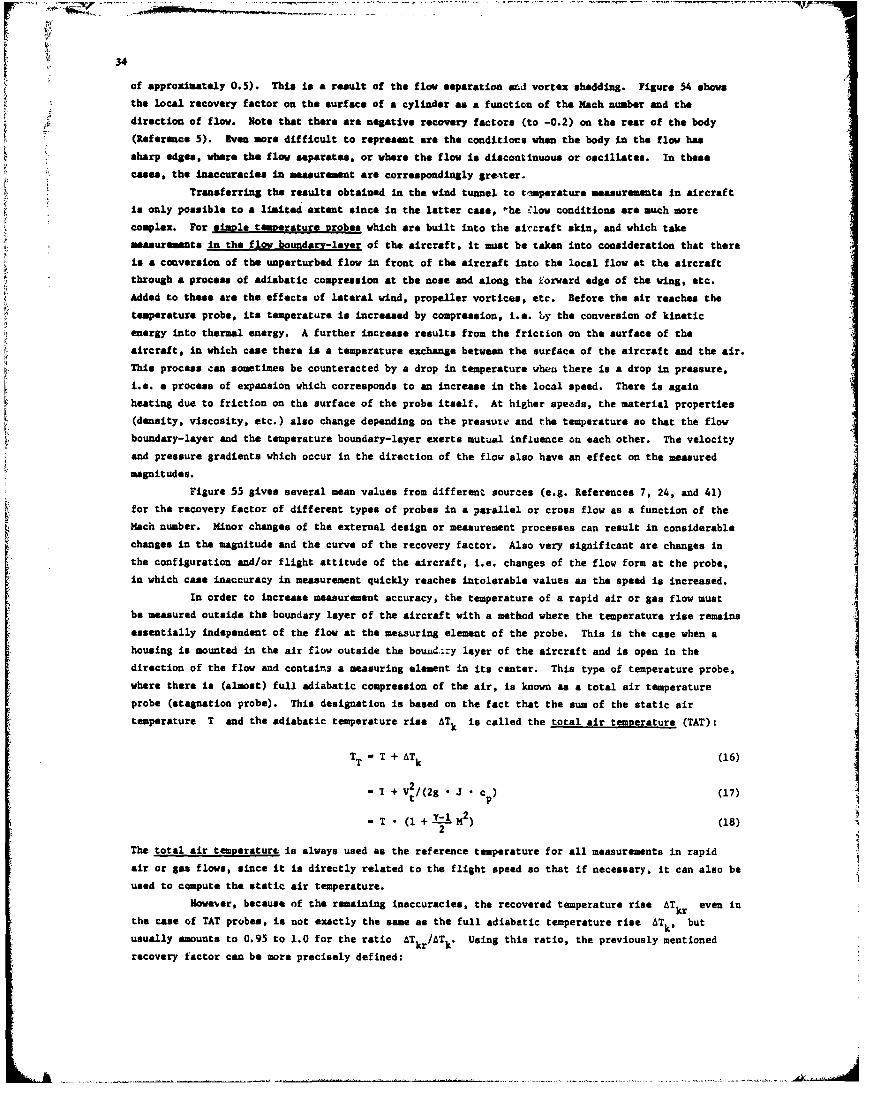
34trmo fa~te ahnme n h

V ~ of approximately 0.5). This is a result of the flow separation &Lnd vortex shedding. Figure 54 shows

diretio offlo. Nte hatthee ae ngatve ecoeryfacors(to-0.2) on the rear of the body

shap ege* whre he lowseprats. r weretheflo Isdiscontinuous or oscillates. In these

Trnfrigterslsobtained in tewntuelotmpruemaseetsin aircraft

is only possible to a limited extent since in the latter case, 'ha -,low conditions are such morecomplex. For simple temperature crobas which are built into the aircraft skin, and which takemeasuremets in the flow boundary-laver of the aircraft, it must be taken Into consideration that there

is a conversion of the unperturbed flow in front of the aircraft into the local flow at the aircraftthrough a process of adiabatic compression at tbe nose and along the iorward edge of the wing, etc.Added to these are the effects of lateral wind, propeller vortices, etc. Before the air reaches thetemperature probe, its temperature is increased by compression, i.e. L.y the conversion of kinetic

energy into thermal energy. A further increase results from the friction on the surface of theaircraft, in which case there is a temperature exchange between the surface of the aircraft and the air.This process can sometimes be counteracted by a drop in temperature when there is a drop in pressure,

i.e. a process of expansion which corresponds to an increase in the local speed. There is againheating due to friction on the surface of the probe itself. At higher speeds, the material properties(density, viscosity, etc.) also change depending on the pressure and the temperature so that the flowboundary-layer and the temperature boundary-layer exerts mutual influence on each other. The velocityand pressure gradients which occur in the direction of the flow also have an effect on the measured

magnitudes.

Figure 55 gives several nean values from different sources (e.g. References 7, 24, and 41)

for the recovery factor of different types of probes in a parallel or cross flow as a function of the

Mach number. Minor changes of the external design or measurement processes can result in considerablechanges in the magnitude and the curve of the recovery factor. Also very significant are changes inthe configuration and/or flight attitude of the aircraft, i.e. changes of the flow form at the probe,in which case inaccuracy in measurement quickly reaches intolerable values as the speed is increased.

in order to increase measurement accuracy, the temperature of a rapid air or gas flow mustbe measured outside the boundary layer of the aircraft with a method where the temperature rise remainsessentially independent of the flow at the measuring element of the probe. This is the case when ahousing is mounted in the air flow outside the bouud,:--y layer of the aircraft and is open in the

direction of the flow and contains a measuring element in its center. This type of temperature probe,where there is (almost) full adiabatic compression of the air, is known as a total air temperature

probe (stagnation probe). This designation is based on the fact that the sum of the static airtemperature T and the adiabatic temperature rise AtTk is called the total air temperature (TAT).*

TT- T +AT k(16)I

2

The total air temperaturt is always used as the reference temperature for all measurements in rapidair or gas flows, since it is directly related to the flight speed so that if necessary, it can also be

used to compute the static air temperature.Howveer, because of the remaining inaccuracies, the recovered temperature rise AT even inkr

the case of TAT prubes, is not exactly the same as the full adiabatic temperature rise AT k$ butusually amounts to 0.95 to 1.0 for the ratio AT [AT Uigti aitepeiul etoe

kr k'Uigti aitepeiul etoerecovery factor can be more precisely defined:

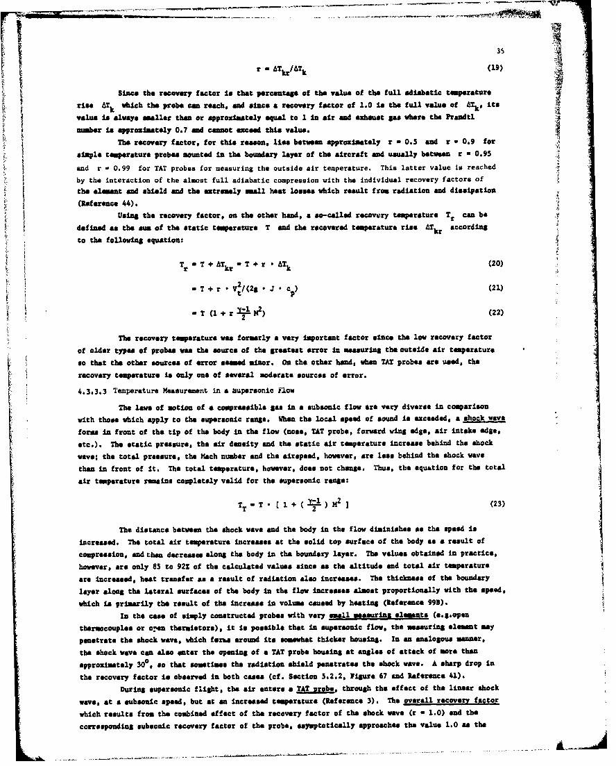
• 35

r - ATkIr/ATk (o9)ft

Since the recovery factor it that percentage of the vaue of the full ad-abtic temperature

rise ATh which the probe cam reach, and since a recovery factor of 1.0 is the full value of ATk, its

value Is always sma]ler than or approximately equal to 1 in air and axhaust gas where the Prandtl

umber is approzimately 0.7 and cannot exceed this value.

The recovery factor, for this reason, lea between approzimstaly r w 0.5 and r - 0.9 for

simple temperature probes mounted In the boundary layer of the aircraft and usually between r a 0.95

and r - 0.99 for TAT probes for measuring the outside air temperature. This latter value is reached

by the interaction of the almost full adiabatic compression with the individual recovery factors of

the element and shield and the aztromely small heat losses which result from radiation and dissipation

(Reference 44).Using the recovery factor, on the other hand, a so-called recovory temperature Tr can be

defined as the sum of the static temperature T and the recovered temperature rise aTkr according

to the following equation:

Tr uT+ATk T + r *ATk (20)

T+r*VtI(2S cp) (21)

T (1+ r 2 (22)

The recovery temperature vas formerly a very important factor since the low recovery factor

of older types of probes was the source of the greatest error in measuring the outside air temperature

so that the other sources of error seemed minor. On the other hand, when TAT probes are used, the

recovery temperature is only one of several moderate sources of error.

4.3.3.3 Temperature Measurement in a bupersonic Flow

The laws of motion of a compressible gas in a subsonic flow are very diverse in comparison

with those which apply to the supersonic range. When the local speed of sound is exceeded, a shock wave

form in front of the tip of the body in the flow (nose, TAT probe, forward wing edge, air intake edge,

etc.). The static pressure, the air density and the static air temperature increase behind the shock

wave; the total pressure, the Msch number and the airspeed, however, are less behind the shock wave

than in front of it. The total temperature, however, does not change. Thus, the equation for the total

air temperature remains completely valid for the supersonic range:

TT" T [ + ( 1) M2 ] (23)

The distance between the shock wave and the body in the flow diminishes as the speed is

Increased. The total air temperature increases at the solid top surface of the body as a result of

compression, and thou decreasm along the body in the boundary layer. The values obtained in practice,

however, are only 85 to 92Z of the calculated values since an the altitude and total air temperature

are increased, heat transfer as a result of radiation also increases. The thickness of the boundary

layer along the lateral surfaces of the body in the flow increases almost proportionally with the speed,

which i. primarily the result of the increase in volume caused by heating (Reference 993).

In the case of simply constructed probes with very smal1 weasurwing elemets (e.g.open

thermocouples or o..em thermistors), it is possible that in supersonic flov, the measuring element may

penetrate the shock wave, which feram around its somewhat thicker housing. In an analogous meanar,

the shock wave can also enter the opening of a TAT probe housing at angles of attack of more than

approximately 30°0 so that sometimes the radiation shield penetrates the shock wave. A sharp drop in

the recovery factor is observed in both cases (of. Section 5.2.2, Figure 67 and Reference 41).

During supersonic flight, the air enters a TAT Probo, through the effect of the linear shock

wave, at a subsonic speed, but at an increased temperature (Reference 3). The overall recovery factor

which results from the combined effect of the recovery factor of the shock wave (r - 1.0) and the

corresponding subsonic recovery factor of the probe, esymptotically approache the value 1.0 as the

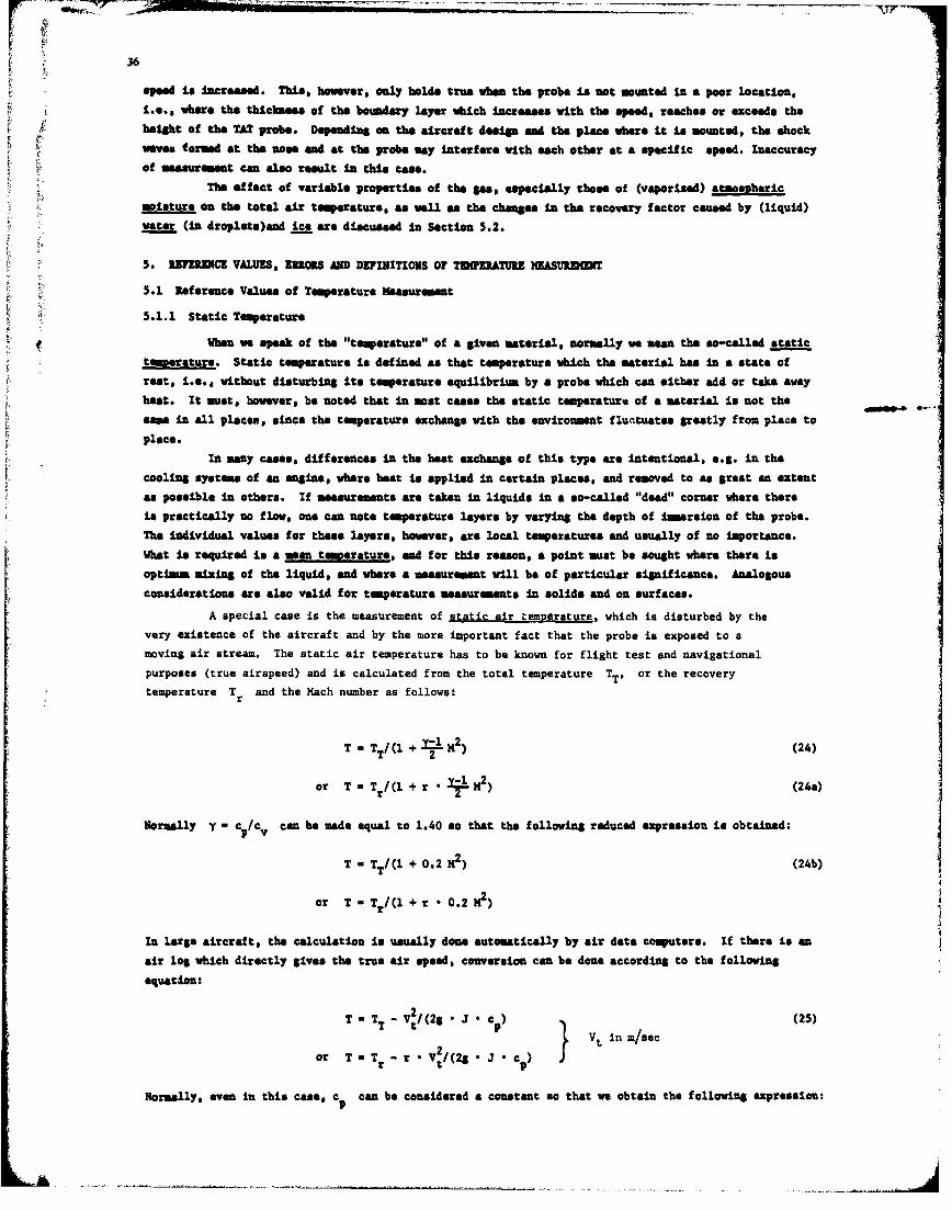
36

speed Is increased. This, howver, only holds true when the probe is not mounted in a poor location,

i.e.s Where the thickness of the boundary layer which increases With the speed, reaches or exceads the

height of the TAT probe. Depending on the aircraft design and the place where it Is mounted, the shock

mvew" formed at the nose end at the probe may interfere with each other at a specific speed. Inaccuracy

of measurement can also result In this case.

The effect of variable properties of the 8as, especially those of (vaporized) atmospheric

moistue on the total aft temperature, as well as the changes in the recovery factor caused by (liquid)

water (in droplets)and ice are discussed in Section 5.2.

5. REFRUENCE VALUES, nORRS AND DEFINITIONS o0 TzonATUIE MEASURMNDT

5.1 Reference Values of Temperature Measurement

5.1.1 Static Tmperature

f hwhen we speak of the "temperature" of a given material, normally we mean the so-called static

toemeratures. Static temperature Is defined as that temperature which the material has In a state of

rest, i.e., without disturbing its temperature equilibrium by a probe which can either add or take avay

heat. It must, however, be noted that in most cases the static temperature of a material is not the

same In all places, since the temperature exchange with the enviromment fu•.tuates greatly from place to

place.

In many cases, differences In the heat exchange of this type are intentional, e.g. in the

cooling systems of an enaine, where heat is applied •n certain places, and removed to as great an extent

as possible In others. If measurements are taken in liquids In a so-called "dead" corner where there

Is practically no flow, one can note temperature layers by varying the depth of Iinersion of the probe.

The Individual values for these layers, however, are local temperatures and usually of no importance.

What is required is a mean temperature, and for this reason, a point mast be sought where there is

optimum lxling of the liquid, and where a measurement will be of particular significance. Analogousconsiderations are also valid for temperature measurements In solids and on surfaces.

A special case is the measurement of static air temperature, which is disturbed by the

very existence of the aircraft and by the more important fact that the probe is exposed to a

moving air stream. The static air temperature has to be known for flight test and navigational

purposes (true airspeed) and is calculated from the total temperature TT, or the recovery

temperature Tr and the Mach number as follows:

T - TT/(l + =1 ) (24)

or T - T /(l + r - -1 H2) (24a)r 2

Normally y - cY/c can be made equal to 1.40 so that the following reduced expression is obtained:

T - TT/(M + 0.2 M2 ) (24b)

or T - T /(I + r * 0.2 M)r

in large aircraft, the calculation is usually done automatically by air data computers. If there Is an

air log which directly gives the true air speed, conversion can be done according to the following

equation:

T - TT - V2 /(28 , J • cp) (25)Vt in n/8ec

or T-T -r. V2/(2S. J. )

Normally, even in this case, c€ can be considered a constant so that we obtain the following expression:

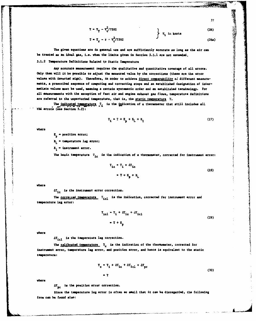
Tm TT V2/7592 (26)

SVt in knots O

TnT, -r V/79 (264k) It

The given equations are Ingee algs and are sufficiently accurate as long asthe air canbe treated asan Ideal pgas i.e. when the limits given in Section 5.3.1 are not exceeded.

5.1.2 Temerature Definitions Related to static Temperature 4

Any accurate measuremnt requires the qualitative and quantitative coverage of all error*.Only then will it be possible to adjust the masaured value by the correctiona (thea. are the errorvaluaa with Inverted sip).* Therefore, In order to achieve direct copargbility ol different meassure-I ~meats, a prescribed sequence of computing and correcting steps and an established designation of Inter-mediate values must be used, maningd a certain systematic order and an established terminology. Forall measurements with the exception of feast air and engine exhaust gas f lows, temperature definition$

are referred to the unperturbed temperatures that is, the static temperature To* The indic~~At pwte tura .ist the ljdication of a thermometer that stilncueal

'tii errors (sea Section 5.2).

Ti T +E + EL+ E (27)

where

I position error;PEL temperature lag error;

E, Instrument error.

The basic temperature T Ic is the indication of a thermometer, corrected for instrument error.

*T *T + AT

aT + +(28)

whereAT1 is the Instrument error correction.

The corr~q temperature Tic is the Indication, corrected for instrument arrcr and *temperature lag error:

Ti0 Ti + ATi + 41Ti

(29)

whereATic is the temperature lag correction.

The calibrated temperature Tc is the Indication of the thermometer, corrected for

Instrument error, temerature lag error, and position error, and hence is equivalent to the statictemperature:

Tc T I+ AT ic + AT ia*+AT PC(30)

whereAT to the position error correction.

PCsince the temperature lag error in often so small that It can be disregarded,* the following

form can be found also:

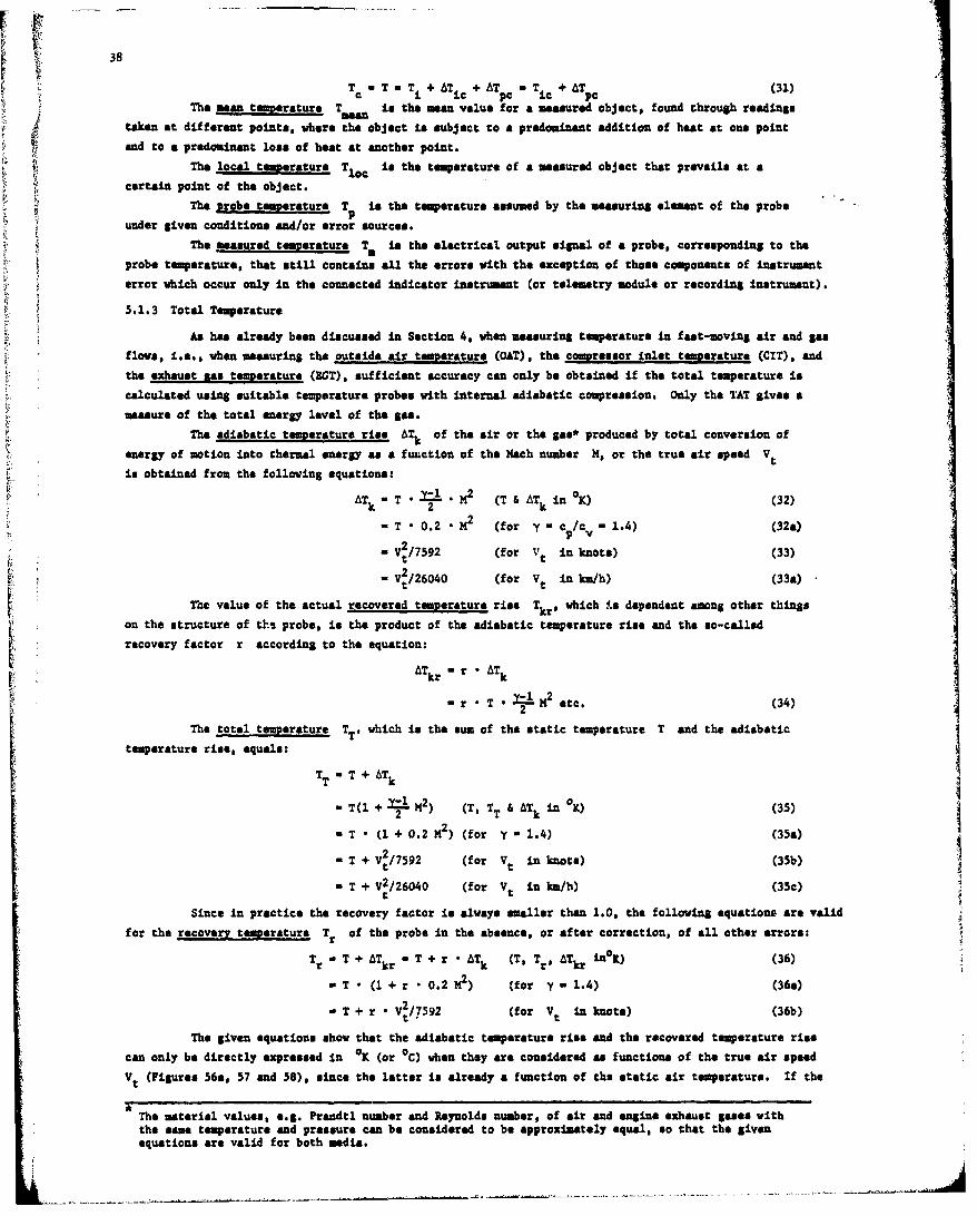
•i 38T TT + AT + AT T + AT (31)

T £ ic PCThe mean tennerature T" is the mean value for a measured object, found through readings

taken at different points, whore the object is subject to a predominant addition of hest at one point

and to a predominant loss of heat at another point.

The local temperature Tio€ is the temperature of a measured object that prevails at a

certain point of the object.

The probe toemperature T1 is the temperature assumed by the measuring element of the probe

under &iven conditions and/or error sources.

The measured tenperature Tm ie the electrical output signal of a probe. corresponding to the

probe temperature, that still contains all the errors with the exception of those componenta of instrument

error which occur only in the connected indicator instrument (or telemetry module or recording instrument).

5.1.3 Total Temperature

As has already been discussed in Section 4, when measuring temperature in fast-moving air and Sas

flows, i.e., when measuring the outside air tegperature (OAT). the compressor inlet temperature (CIT). and

the exhaust gas temperature (RaT), sufficient accuracy can only be obtained if the total temperature is

calculated using suitable temperature probes with internal adiabatic compression. only the TAT Sivas a

measure of the total energy level of the Sga.

The adiabatic tmpaerature rise ATk of the air or the Sae* produced by total conversion of

energy of motion into thermal energy as a function of the Mach number M, or the true air speed Vt

is obtained from the following equations:

AT T K (T &AT in OK) (32)k 2 k

-T • 0.2 M2 (for y c/c - 1.4) (320)p V

- /7592 (for Vt in knots) (33)

- V2/26040 (for Vt in km/h) (33a)

The value of the actual recovered temperature rise TkrP which .s dependent among other things

on the structure of tho probe, is the product of the adiabatic temperature rise and the so-called

recovery factor r according to the equation:

ATkr w r - ATkm r • ,o-r *T OX~H tc. (34)

2The total temperature TT. which is the sum of the static temperature T and the adiabatic

temperature rise, equals:

TT m T +A Tk

- T(l + =1_ M2 ) (T, TT&ATkin K) (35)

- T • (1 + 0.2 M2 ) (for y 1.4) (35a)

- T+ V2 /7592 (for Vt in knots) (35b)

a T + V2/26040 (for Vt in km/h) (35c)t

Since in practice the recovery factor is always smaller than 1.0, the following equations are valid

for the recovery temperature Tr of the probe in the absence, or after correction, of all other errors:

Tr T + ATkr - T + r * ATk (T, Tra ATkr inOK) (36)

w T * (1 + r • 0.2 M2 ) (for y - 1.4) (36&)

w T + r • V'/7592 (for Vt in knots) (36b)

The given equations show that the adiabatic temperature rise and the recovered temperature rise

can only be directly expressed in OK (or oC) when they are considered as functions of the true air speed

Vt (Figures 56&0 57 and 58), since the latter is already a function of ths static air temperature. If the*

The material values, e.g. Prsndtl number and Reynolds number, of air and engine exhaust gases withthe sane temperature and pressure can be considered to be approximately equal, so that the givenequations are valid for both media.

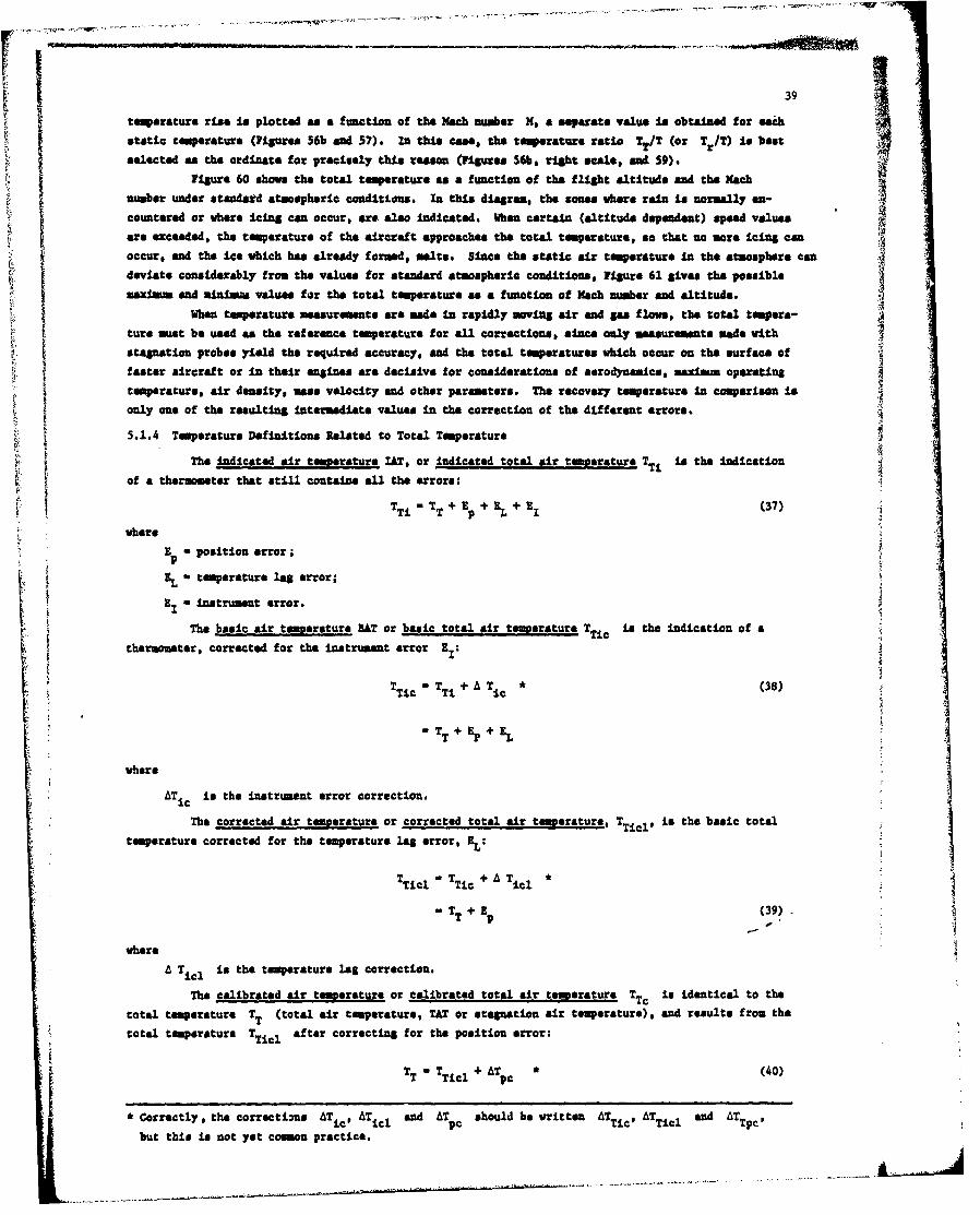
39

tesperature rise is plotted as a function of the Mach number M, a separate value Is obtainsd for

static temperature (Figures 56b and 57). In this cae, the temperature ratio TT/T (or Tr/T) is best

selected as the ordinate for precisely this reason (Figures 56b, right scale, and 59).

Figure 60 shove the total teperatures a function of the flight altitude and the Xach

number under standad atmospheric conditions. In this diagram, the son"s where rain is normally en-

countered or where icing can occur, arte also Indicated. When certain (altituds dependent) speed values

are exceeded, the temperature of the aircraft approaches the total temperature, so that no more icing can

occur, and the iee which has already formed, melts. Since the static air temperature in the atmosphere can

deviate considerably from the values for standard atmospheric conditions, Figure 61 gives the possible

maximumm and minima values for the total temperature as a function of Mach number and altitude.

When temperature measurements are made in rapidly novin air and gas flows, the total tempera-

ture must be used as the reference temperature for all corrections,.i nc only measurements made withstagnation probes yield the required accuracy, and the total temperatures which occur on the surface offaster aircraft or in their engines are decisive for considerations of aerodynamics, -amum operating

temperature, air density, mass velocity and other parameters. The recovery temperature in comparison is

only one of the resulting Intermediate values In the correction of the different errors.

5.1.4 Temperature Definitions Related to Total Temperature

The Indicated air temoerature IAT, or indicated total air toersature TTI is the Indication

of a thermometer that still contains all the errors:

- TT+ E + E (37)Tni T pI~E

where

3- position error;

EL - temperature US error;

E,- Instrument error.

The basic air temperature BAT or basic total air temperature TTt€ is the indication of a

thermometer, corrected for the inatrument error E I

T -T * (38)TT•c TTi A Tic

!4

where -T

ATi•c is the instrument error correction.

The corrected air temperature or corrected total air temperature, TTicl, is the basic total

temperature corrected for the temperature lag error, ITTiC- TTic +A TicL

TT + 1 (39)

where

L T a Is the temperature lag correction.

The calibrated air temperature or calibrated total air temperature TT, is identical to the

total temperature TT (total air temperature, TAT or stagnation ait temperature), and results from the

total temperature TTic, after correcting for the position error:

TT TTicl p AT * (40)

• Correctly, the corrections ATic, AT icl and AT c should be written ATTIC' ATTi•l and ATTIP

but this is not yet common practice.

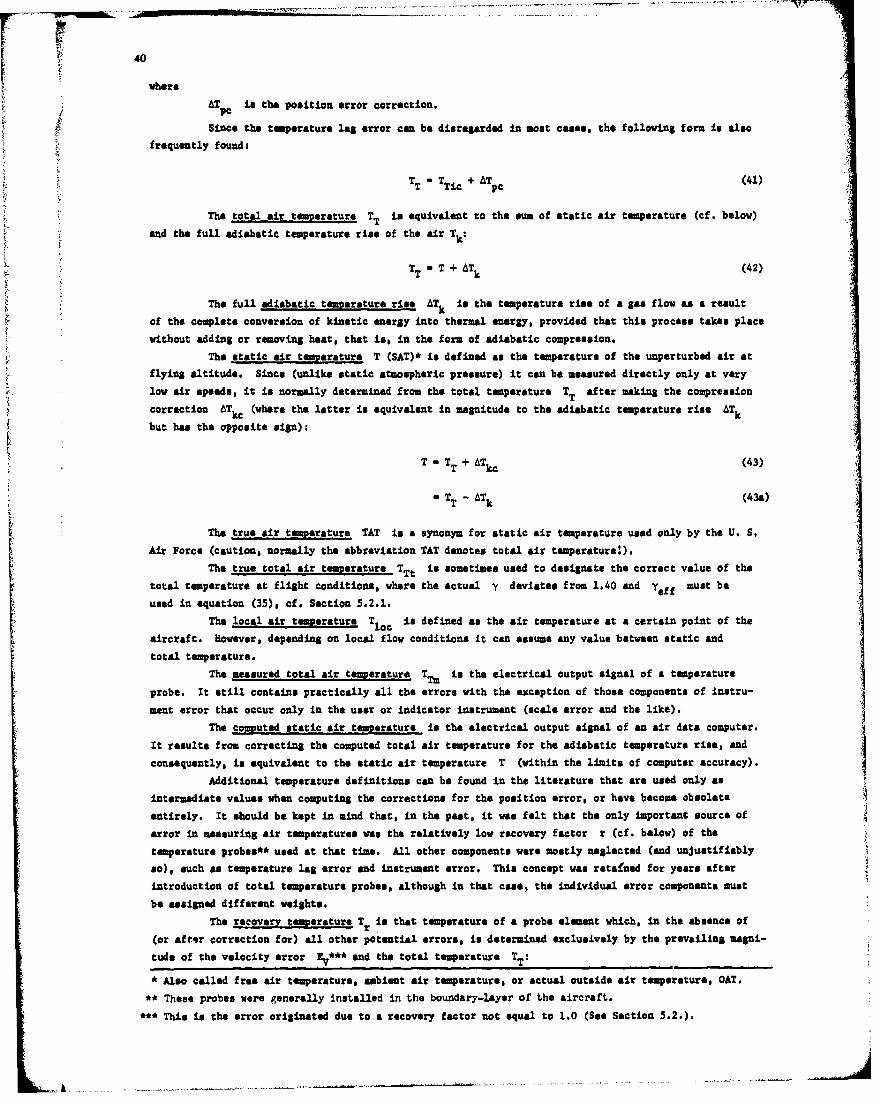
40

ATP in the position error correction.

Since the temperature lag error can be disregarded in most cases, the following form is also

TT TTic +Apc

and the full adiabatic temperature rise of the airT

The full adiabatic temoerature rise AT, is the temperature rise of a gae flow as a result

of the complete conversion of kinetic energy into thermal energy, provided that this process takes place

without adding or removing heat, that is, in the form of adiabatic compression.

The static air temperature T (SAT)* is defined as the temperature of the unperturbed air at

flying altitude. Since (unlike static atmospheric pressure) It can be measured directly only at very

low air sod, it in normally determined from the total temperature Tr after making the compression

correction ATc (where the latter is equivalent in magnitude to the adiabatic temperature rise ATk

but bas the opposite sign):

T T T + ATk (43)

TT- AT (3a

The true air temperature TAT is a synonym for static air temperature used only by the U. S.

Air Force (caution, normally the abbreviation TAT denotes total air temperature!).

The true total air temperature Tt is sometimes used to designate the correct value of the

total temperature at flight conditions, where the actual y deviates from 1.40 and yefmust be

used in equation (35), cf. Section 5.2.1.

The local air teM~erature T loc is defined as the air temperature at a certain point of the

aircraft. However, depending on local flow conditions it can assume any value between static and

total temperature.

The measured total air temperature T~m is the electrical output signal of a temperature

probe. It still contains practically all the errors with the e"ception of those components of instru-

ment error that occur only in the user or indicator instrument (scale error and the like).

The computed static air temperature is the electrical output signal of an air data computer.

It results from correcting the computed total air temperature for the adiabatic temperature rise, andIconsequently, is equivalent to the static air temperature T (within the limits of computer accuracy).

Additional temperature definitions can be found in the literature that are used only as

intermediate values when computing the corrections for the position error, or have become obsolete

entirely. It should be kept in mind that, in the past, it was felt that the only Important source of

error in measuring air temperatures was the relatively low recovery factor r (cf. below) of the

temperature probes** used at that time. All other components were mostly neglected (and unjustifiably

so), such as temperature lag error and instrument error. This concept was retafoed for years after

introduction of total temperature probes, although in that case, the individual error components must

be "ssigned different weights.

The recovery temperature T ris that temperature of a probe element which, in the absence of

(or aft~er correction for) all other potential errors, is determined exclusively by the prevailing magni-

tude of the velocity error end the total temperatureTT

*Also called free air temperature, ambient air temperature, or actual outside air temperature, OAT.

**These probes were generally installed in the boundary-layer of the aircraft.

**This is the error originated due to a recovery factor not equal to 1.0 (See Section 5.2.).

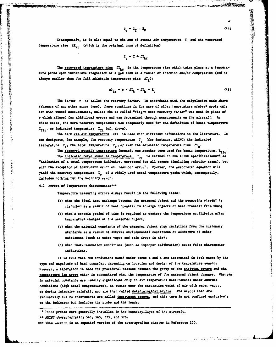
41

Tr- TT (44)

Consequently, it is also equal to the sum of static air temperature T and the recovered

temperature rise ATkr (which is the original type of definition)

T iTkr

TTh T r ATkr

The reuovered temperature rise Tkr is the temperature rise which takes place at a tempera-

cure probe upon Incomplete stagnation of a gas flow as a result of friction and/or compression (and is

k- always smaller than the full adiabatic temperature rise ATk):

F- ATkr r • ATk -ATk EV (45)

The factor r is called the recovery factor. In accordance with the stipulation made above

(absence of any other error type), these equations in the case of older temperature probes* apply only

for wind tunnel measurements, unless the so-called "flight test recovery factor" was used in place of

r which allowed for additional errors and was determined through measurements on the aircraft. In

these cases, the taem recovery temperature was frequently used for the definition of basic temperature

- TTic, or Indicated temperature TTi (cf. above).

The term ran air teS erLture RAT is used with different definitions in the literature. It

can designate, for example, the recovery temperature Tr (for instance, ARINC) the indicated

temperature TiV the total temperature TT, or even the adiabatic temperature rise ATh.

The observed outside temoerature formerly was another term used for basic temperature, TTic'

The indicated total absolute temperature TTi is defined in the ARINC specifications** as

"indication of a total temperature indicator, corrected for all errors (including velocity error), but

with the exception of instrument error and read-out error". However, the associated equation will

yield the recovery temperature Tr of a widely used total temperature probe which, consequently,

Includes nothing but the velocity error.

5.2 Errors of Temperature Measurements***

Temperature measuring errors always result in the following cases:

(a) when the ideal heat exchange between the measured object and the measuring element is

disturbed as a result of heat transfer to foreign objects or heat transfer from themI

(b) when a certain period of time is required to restore the temperature equilibrium after

temperature changes of the measured object;

(c) when the material constants of the measured object show dsviations from the customary

standards as a result of extreme environmental conditions or admixture of other

substances (such so water vapor and rain drops in air);

(d) when instrumentation conditions (such as improper calibration) cause false thermometer Iindications.

It is true that the conditions named under item a and b are determined in both cases by the

type and magnitude of heot transfer, depending on location and design of the temperature sensor.

Piwever, a separation is made for procedural reasons between the group of the position errors and the

temperature lag error which is encountered when the temperature of the measured object changes. Changes

ILn material constants are usually significant only in air temperature measurements under extreme

conditions (high total temperatures), in states near the saturation point of air with water vapor,

or during intensive rainfall, and are then called meteorological errors. The errors that are

axclusivaly due to instruments are called instrumant errors, and this term is not confined exclusively

to the indicator but includes the probe and the leads.

* These probes were generally installed in the boundary-layer of the aircraft.

•* ARINC characteristics 545, 565, 575, and 576.

•** This section is an expanded version of the corrrsponding chapter in Reference 100.

' ', •4.. .. . . . . . ... .. . . .+.. . ... . . .. .. . . . . .. . . . . . . .. . .. . . .- ... . . . . .. . . . . '- - -" • ' = • . . . . . . .. . .

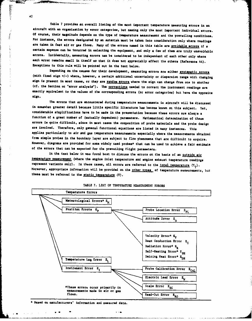
acaT able 7 provides an overall listing of the most important temperature measuring errors in an

k Of ~course&te ir magnitude depends on the type of temperature measurement and the prevailing conditions.For instance. the error@ designated by an asterisk must be taken Into consideration only where readingsare taken In fast air or gas flows. Many of the errors named In this table are avoidable errors if acertain expense can be incurred in selecting the equipment, and only a few of them are truly unavoidableerrors. Incidentally, measuring errors can be considered to be independent of each other only whereeach error remains small In Itself so that it does not appreciably affect the others (Reference 44).Exceptions to this rule will be pointed out in the text below.

Depending on the causes for their development, measuring errors are either systematic errors(with fixed sign +/-) where, however, a certain additional uncertainty or dispersion range with changingsign is present In most cases, or they are random errors where the sign can change from one to another(of. the Section on "error analysis"). The corrections needed to correct the instrument readings areexactly equivalent to the values of the corresponding errors (or error categories) but have the oppositesipn.

The errors that are encountered during temperature measurements in aircraft will be discussedin somewhat greater detail because little specific literature has become known on this subject. Yet,considerable simplifications have to be made in the presentation because these error$ are always afunction of a great number of (mutually dependent) parameters. Mathematical determination of theseerrors Is quite difficult, since In most cases the composition of probe materials and the probe design

are involved. Therefore, only general functional equations are listed in many instances. Thisapplies particularly to air and gas temperature measurements especially where the measurements obtainedfrom simple probes in the boundary layer-are subject to flow phenomena that are difficult to acquire.However, diagrams are provided for some widely used probes* that can be used to achieve a fair estimateof the errors that can be expected for the prevailing flight parameters.

in the text below it was found beat to discuss the errors on the basis of an outside airtemperature measurement (where the engine inlet temperature and engine exhaust temperature readingsrepresent variants only). In these cases, all errors are referred to the total temperature (TT)'Moreover, appropriate information will be provided on the other type ftmeauemaueeti uthese must be referred to the static temperature (T).

TABLE 7.* LIST OF TEMPERATURE MEASUREMENT ERRORS

Temperature Errors

Meteorological Erru*M

Posit ion Errors E~ Probe Location Error EL

Attiude ErrorrEE

A~hse rroui ccu prmarlylncale Error*Emeasurements-C mae nai r aflows.10

RedOt Error*

* ~ ~ ~ ~ ~ ~ ~ ~ ~ ~ aito Erased oEmnfcues nomainadmaue aa

. *~ 0 'R

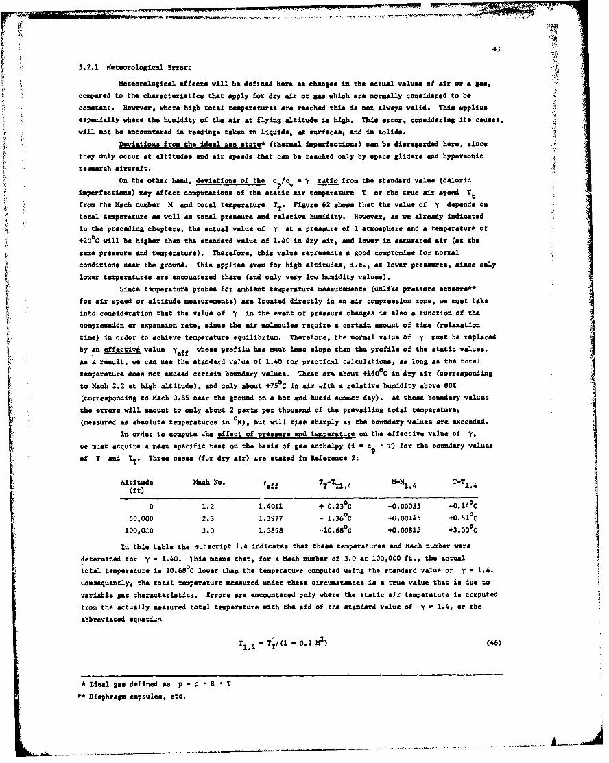
43

5.2.1 Keteorological Erroru trme

Meteorological effects will be defined here as changes in the actual values of air or a Sam,

compared to the characteritics that apply for dry air or ias which are normally considered to be

constant. However, where high total temperatures are reached this is not always valid. This applies

especially where the humidity of the air at flying altitude in high. This error, considering its causes.

will not be encountered in readings taken in liquids, at surfaces, and in solids.

Deviations from the ideal gas states (thermal imperfecticns) can be disregardad here, since

they only occur at altitudes and air speeds that can be reached only by space gliders and hypersonic

research aircraft.

On the other hand, deviations of the c /c - y ratio from the standard value (caloricpv -

imperfections) may affect computations of the static air teperature T or the true air speed Vt

from the Mach number M and total temperature TT. Figure 62 shows that the value of y depends on

total temperature as well as total pressure and relative humidity. However, as we already indicated

in the preceding chapters, the actual value of y at a pressure of 1 atmosphere and a temperature of

+20 0 C will be higher than the standard value of 1.40 in dry air, and lower in saturated air (at the

same pressure and temperature). Therefore, this value represents a good compromise for normal

conditions near the ground. This applies avan for high altitudes, i.e., at lower pressures, since only

lower temperatures are encountered there (and only very low humidity values).

Since timperature probes for ambient temperature measurements (unlike pressure sensors**

for air speed or altitude measurements) are located directly in an air compression zone, we must take

into consideration that the value of y In the event of pressure changes is also a function of the

compressiOn or expansion rate, since the air molecules require a certain amount of time (relaxation

time) in order to achieve temperature equilibrium. Therefore, the normal value of y must be replaced

by an effective value yef whose proftia has muck less slope than the profile of the static values.

As a result, we can use the standard vs!.ue of 1.40 for practic-l calculations, as long as the total

temperature does not exceed certain boundary values. These ar* about +160 C in dry air (corresponding

to Mach 2.2 at high altitude), and only about +75°C ia air with 9 relative humidity above 80%

"corresponding to Mach 0.85 near the ground on a hot and humid summer day). At these boundary values

the errors will amount to only about 2 parts per thousand of the prevailing total temperatures

(measured as absolute temperatures in OK), but will rise sharply as the boundary values are exceeded.

In order to compute .9he effect of pressure and temperature on the effective value of y,

we must acquire a mean specific heat on the basis of &to enthalpy (i a cp . T) for the boundary values

of T and TT. Three cases (fur dry air) 6re stated in Reference 2:

Altitude Mach No. Yff T T-TT1.4 M-M1.4 T-TI.4(ft)

0 1.2 1.4011 + O.23 0C -0.00035 -0.14 0 C50,000 2.3 1.1977 - 1.360 C +0.00145 +0.51 0 C

100,000 3.0 1. •898 -10.68 C +0.00815 +3.00 C

Iu this table the subscript 1.4 indicates that these temperatures and Mach number were

determined for y - 1.40. This means that, for a Mach number of 3.0 at 100,000 ft., the actual

total temperature is 10.68°C lower then the temperature computed using the standard value of y - 1.4.

Consequently, the total temperature measured under these circumstances is a true value that is due to

variable gas characteristics. Errors are encountered only where the static ai.r temperature is computed

from the actually measured total temperature with the aid of the standard value of y 1.4, or the

abbreviated eqvatL..%

T1. 4 - TT/(l + 0.2 M2) (46)

* Ideal gas defined as p =p * R T T

* Diaphragm capsules, etc.

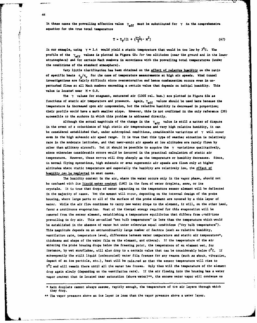
44

In these costs tre dprevailin effective value Yeff mr t be substituted for y in the omprehensiveJ equation for the true total temperature

ST.T/[1 + y M](47)

In our example, using y - 1.4 would yield a static t erature that would be too low by 3°C. The

profile of the yoff values i. plotted in Figure 62A for two altitudes (near the ground and in the lower

stratospheie) and for certain Mach numbers In accordance with the prevailing total temperatures (under

the conditiont of the standard atmohmtre).•. ~Very little clar~ification has been obtained on the effect of relative humidity an the ratio

of spepcific heats c v for the came of temperature esuremets at high air speeds. Wind tunnelinvestigations are fairly difficult since oversaturatlon and hence condensation occurs even In un-

perturbed flows at all Mach numbers exceeding a certain value that depends on initial humidity. This

value is located near M w 0.8.

The y values for stagnant, saturated air (lOOZ rel. hum.) are plotted in Figure 62a as

functions of static air temperature and pressure. Again, Yoff values should be used here because the

temperature is increased upon air compression, but the relative humidity is decreased in proportion;

their profile would have a much smaller slope. However, this is not confirmed in the only reference (39)

accessible to the authors in which this problem is addressed directly.

Although the actual magnitude of the change in the yeff value is still a matter of dispute

in the event of a coincidence of high static air temperatures and very high relative humidity, it can

be considered established that, under subtropical conditions, considerable variations of y will occur

even in the high subsonic air speed range. It is true that this type of weather situation is relatively

rare in the moderate latitudes, and that near-sonic air speeds at low altitudes are rarely flown by

other than military aircraft. Yet it should be possible to acquire the y variations qualitatively,

since otherwise considerable errors would be incurred in the practical calculation of static air

temperature. However, these errors will drop sharply as the temperature or humidity decreases. Since,

in normal flying operations, high subsonic or avon supersonic air speeds are flown only at higher

altitudes where static temperature and especially the humidity are relatively low, the effect of

humidity can be neglected in most cases.

The humidity content in the air, where the water occurs only in the vapor phase, should not

be confused with its liquid water content (LWC) in the form of water droplets, snow, or icecrystals. It is true that drops of water im•pacting on the temnperature sensor element will be deflected

in the majority of cases. Yet the moment will occur, depending on the internal design of the probe

housing, where large parts or all of the surface of the probe element are covered by a thin layer of

water. While the air flov continues to carry new water drops to the element, it will, on the other hand,

favor a continuous evaporation. Host of the thermal energy required for this evaporation will be

removed from the sensor element, establishing a temperature equilibrium that differs from Lnndition8

prevailing in dry air. This so-called "wet bulb temperature" is less than the temperature which would

be established in the absence of water but under otherwise equal conditions ("dry bulb temperature").

This magnitude depends on an extraordinarily large number of factors (such as relative humidity,

ventilation rate, temperature level, difference between water temperature and static air temperature*,

thickness and shape of the water film on the element, and others). If the temperature of the air

entering the probe housing drops below the freezing point, the temperature of an element wet, for

instance, by wet snowflakes, will also drop to a certain value that can be considerably below 0C. If

subsequently the still liquid (undercooled) water film freezes for any reason (such as shock, vibration,

impact of an ice particle, etc.), heat will be releised so that the sensor temperature will rise to

O°C and will remain there until all the water has frozen. Only then will the temperature of the element

drop again slowly (depending on the ventilation rate). If the air flowing into the housing has a water

vapor content that is located near saturation (above water)**, the excess water vapor will condense on

* Rain droplets cannot always assume, rapidly enough, the temperature of tlie air layers through whichthey drop.

5* The vapor pressure above an ice layer is less then the vapor pressure above a water layer.

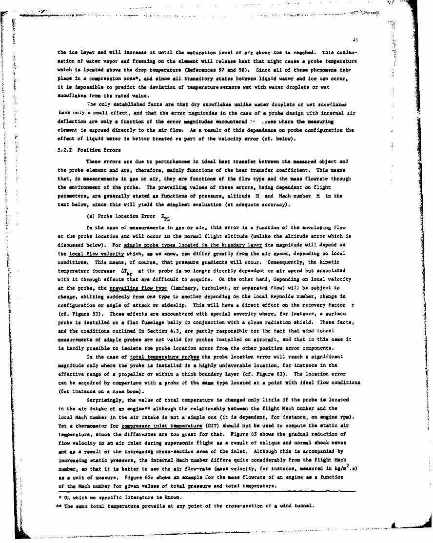
I IV45

the Ice layer and will Increase it until the saturation level of air above ice Is reached. This conden-

sation of water vapor and freezing on the element will release heat that might cause a probe temperature

which is located above the drop temperature (Raferences 97 and 98). Since all of these phenomena take

place in a compression zone*, and since all transitory states between liquid water and Ice can occur,

it is Impossible to predict the deviation of temperature sensors vat with water droplets or wet

snowflakes from its rated value.The only established facts are that dry snowflakes unlike water droplets or vet snowflakes

have only a small effect, and that the error magnitudes in the case of a probe design with internal air

deflection are only a fraction of the error magnitudes encountered :- .-obes uhere the measuring

element is exposed directly to the air flow. A~s a result of this dependence on probe configuration thet effect of liquid water is better treated rs part of the velocity error (cf. below).

5.2.2 Position Errors

These errors are due to parturbances in ideal heat transfer between the measured object and

the probe element and are, therefore, mainly functions of the heat transfer coefficient. This means

that, in measurements in gas or air, they are functions of the flow type and the mass flowrate through

the environment of the probe. The prevailing values of these errors, being dependent on flight

parameters, are generally stated as functions of pressure, altitude H and Mach number M in the

text below, since this will yield the simplest evaluation (at adequate accuracy).

(a) Probe location Error P

in the case of measurements in gas or air, this error is a function of the enveloping flow

at the probe location and will occur in the normal flight altitude (unlike the altitude error which is

discussed below). For simple probe types located in the bc.undary layer its magnitude will depend on

the local flow velocity which, as we know, can differ greatly from the air spend, depending on local

conditions. This means, of course, that pressure gradients, will occur. Consequently, the kineticIitemperature increase AT kr at the probe is no longer directly dependent on air speed but associatedwith it through effects that are difficult to acquire. On the other hand, depending on local velocity

at the probe. the prevailing flow type (lamiuary, turbulent, or separated flow) will be subject to

change, shifting suddenly from one type to another depending on the local Reynolds number, change inI configuration or angle of attack or sideslip. This will have a direct effect on the recovery factor r(cf. Figure 53). These effects are encountered with special severity where, for instance, a surface

probe Is installed on a flat fuselage belly in conjunction with a close radiation shield. These facts,and the conditions outlined in Section 4.3, are partly responsible for the fact that wind tunnel

measurements of simple probes are not valid for probes installed on aircraft, and that in this case it

is hardly possible to isolate the probe location error from the other position error components.

In the case of total temperature Brobes the probe location error will reach a significant

magnitude only where the probe is installed in a highly unfavorable location, for instance in theI

effective range of a propeller or within a thick boundary layer (cf. Figure 63). The location error

can be acquired by comparison with a probe o~f the same type located at a point with ideal flow conditions

(for instance on a nose boom).

Surprisingly, the value of total temperature is changed only little if the probe is located

in the air intake of an engine** although the relationship between the flight Mach number and the

local Mach number in the air intake is not a simple one (it is dependent, for instance, on engine rpm).

Yet a thermometer for compressor inlet temperature (CIT) should not be used to compute the static air

temperature, since& the differences are too grant for that. Figure 65 shows the gradual reduction of

flow velocity in an air inlet during supersonic flight as a result of oblique and normal shock waves

and as a result of the increasing cross-section area of the inlet. Although this is accompanied by

increasing static pressure, the internal Mach number differs quite considerably from the flight Mach

number, so that it is better to use the air flow-rate (mass velocity, for instance, measured in kg/in2 s)

as a unit of measure. Figure 62c shows an example for the mass flowrate of an engine as a function

of the Mach number for given values of total pressure and total temperature.

0-O~ which no specific literature is known.

**The ssmn total temperature prevails at any point of the cross-section of a wind tunnel.

46

For rapidly moving gases, as in inlets, not only velocity gradients are found but temperature

gradients as well, and their distribution will be dependent on a very large number of parameters (such

as inlet geometry, air inlet velocity, temperature difference between wall and air,* Reynolds number,

Prandtl number and others). Consequently, even where a TAT probe (for a CIT reading) is installed on an

inlet wall, we must keep in mind that in the event of fast climbing or descending flight the CIT

indication may lag considerably behind as a result of the temperature exchange between the air end the

inlet wall (lag error) until the wall has adjusted to the new temperature equilibrium. Therefore, in

order to acquire accurate readings durinig flight tests, especially in the air inlets of VTOL aircraft.

a number of temperature probes are distributed evenly over the cross-sectionT (cf. Figure 66).The probe location error can be cefined approximately by:

EL "IT' KF, KPL) (48)

meaning that it is a function of total pressure and static pressure at the probe location, the design

characteristics of the probe (K7 ), and the airflow characteristics at the probe location (.,)

Sometimes the term installation error is falsely used as a synonym for location error.

Actually, however, the installation error designates only the difference between the location errors

of identically equipped aircraft of the same production series. It is determined primarily by

production tolerances which have the result that aircraft of identical appearance can have different

flow relationships at the probe.

Where neasurements are taken in liguids a considerable probe location error can develop if

the probe is installed, for instance, at a "dead" point of the tank where no notion exists and where a

temperature can develop that differs from the temperature of the remaining liquid. Likewise, a probe

location error can develop during measurements on surfaces and in solid bodies, if an unfavorable

Flocation is selected for the probe where the desired heat exchange with the measured object is obstructedbut where the heat exchange with foreign objects is favored as a result of this location.

(b) Attitude Error EaThis error will occur only when the probe is exposed to a non-parallel flow. Consequently,

relatively large angles of attack (a) and angles of sideslip (B) will cause this error in probes

for air temperature measurements. The older probe configurations react quite clearly to angles of

about ±50, and in cacc of TAT probes with the deicing system in operation, an angle of +10' (often more

than ±20* if the deicing system is turned off) must be exceeded before the reduced local flow of the

probe element appears as an air speed reduction, leading to a reduction in the temperature indication

(cf. Figure 64). When the deicing system is turned on this is partially compensated or even over-

compensated by an increase of the self-heating error and deicing heat error. cf. below.

The attitude error involved in TAT readings in fast aircraft is usually so small that it ce

be neglected. However, in the case of extremely low-speed aircraft a strong crosswind can render the

encircling flow of the aircraft highly Instable. VTOL aircraft and helicopters frequently have very

large angles of yaw and during vertical ascent or descent, even purely vertical local flows, that can

have a high degree of vorticity as a result of recirculation effects, rotor effects, and the like. In

that case, very large errors and large error dispersion must be expected in outside air temperature

measurements unless an indicator with extremely low probe self-heating characteristics is used (and

unless any probe deicing system that may be installed can be turned off).

The attitude error can be defined by:

E a f(n, B, Ko M ) (49)

where

K represents a factor that is dependent on the probe design.aLAni attitude error during measuremeats in liquids occurs, for instance where, in the case of

stem probes, the flow encounters the foot of the probe first, changes its temperature, and only then

reaches the temperature-sensitive top of the probe. This type of error doss not occur during

measurements on surface and in solid bodies.

it(c) Velocity Error .

This error which occurs only during measurements in fast air or gas flows states the amount

by which the recovery temperature T of a probe remains below the total temperature Twhich isr T

equivalent to the difference between full adiabatic temperature increase ATadaqie eprtrincrease AT~c

EV TT -T ATc- ATc (50)

Before defining the dependence of the velocity error on air speed in more detail some additional terms

must be explained:

(c-1) The recovery factor r is nondimensional and designates, as previously mentioa d, the

ratio of the temperature rise acquired by the probe to the full adiabatic temperature rise.

r =ATkr/ATk (Tr T)/(TT T) (51)

ATk r ATc (52)

In air and in engine exhaust gases it is always smaller than 1.0*, even though some instrument readings

appear to contradict this - probably because other effects were not fully covered. In the case of

simple Probes installed in the boundary laver of the airctaft, the recovery factor will be between the

limit values of approximately r - 0.5 and r - 0.9 (cf. Figure 55),* where a measuring uncertainty

between +0.03 r and +0.1 r can occur if the airflow moves parallel to the probe surface. In the

case of stem probes placed in a lateral flow, this instrument dispersion can be even considerably

greater. The recovery factor for simple probes in the boundary layer of a wind tunnel could be defined

by:

r f(Vt, Pr, Re, kc, K,,M KPL . . .) (53)

As the local flow conditions in a wind tunnel and on the skin of an aircraft are quite different

(cf. Section 4.3.3.2), the tern "flistht test recovery factor" was created:

V2 localrfih tes -- (1-r0 (54)

f i h te tVt2 aircraft

Where this factor was acquired through measurements on the aircraft, it automatically incorporates

other components of the position error (such as the probe location error) so that a family of curves

dependent on altitude or aircraft weight (or angle of attack) resulted in place of a single curve

dependent on velocity.

In the case of good total temperature probes the recovery factor is practically only a

function of the Mach number M and the design characteristics KK, of the probe:

r - f(H, K(~ (55)

It is true that this definition, too, incorporates certain components of the heat conduction error and

radiation error (cf. below). However, in the case of TAT probes all terms involved in the air speed

error or the recovery temperature can be treated as if all errors were independent of each other. It

is seen from Figure 68 that the recovery factor of TAT probes for outside air temperature readings in

the subsonic range (up to about Mach 0.7) is located near a constant value between 0.96 and 0.99;

certain models with open wire elements have even better characteristics. The dispersion between

individual probes of the same type should amount to about +0.015 r in the air speed range below Mach

0.7 (cf. the dispersions of simple probes stated above). Sometimes, slightly lower values of r will

be encountered in the case of TAT probes for engine air inlet temperature measurements. This is

primarily due to the requirements for low probe height, high vibration stability, and others**. In the

*In the case of other gases and liquids with higher Prandtl number, values above 1.0 are possible.

**One extreme sample is the Type 153 AC probe with recovery factors between r -0.7 and 0.8.

48

c.aa of TAT probes for outside air tempsrature measurements the recovery factor increases sharply abover: approximately Mach 0.7, since the internal flow velocity in the probe remains constant above this value.

Under these circumstances it is better to use a different tern:

(c-2) The recovery error is nondimensional, too, and states the ratio of velocity error to

total teperature

n (TT - Tr)/TT "V/TT or (56)

E- i• " " TT (57)

* Figurea 67 and 68 show that, in the case of TAT probes, the recovery error can be considered almost

constant in the supersonic range (this is the manufacturer's information). However, a more detailed

investigation will show that, while the total temperature ahead and behind the shock wave remains

constant in supersonic flight, all other values (Mach number, velocity, pressure, etc.) are subject to

change. As a result of shock wave formation in front of the probe Inlet, the air flow enters at

increased temperature, but with a subsonic Mach number that is a function of the flight Mach number

* i(cf. Figure 69). The shock wave itself can be assigned a recovery factor of r n 1.0. The prevailing

subsonic recovery factor r1 of the probe mast be added. The supersonic recovery factor r' that

* :results from these two steps can be described as follows (according to Reference 3):

1 - r' [1- .-1 ) * [1 2

41 ~iM 4 (58) -1

where the supersonic flight Mach number must be substituted for M (cf. Figure 69). Thus assuming

a constant subsonic recovery factor, a sharply defined maximum of the recovery error is obtained(and hence of the velocity error) at Mach 1.0 which decreases at first rapidly and then more slowly

with increasing Mach uumber and will start to rise again slowly beyond Mach 2.5. However, assuming

that the recovery factor will rise at Mach numbers between 0.7 and 1.0 (at the probe inlet), this

stipulation will have an effect in the supersonic range between Mach 1.0 and 1.4 also (where the

Mach number drops behind the shock wave from Mach 1.0 to about Mach 0.7). As a result, the maximumof the velocity error is considerably flattened so that the values of the theoretical consideration

differ only little from the values that stipulate a constant supersonic recovery error (relative

value in percent of total temperature).

Instrument readings where the velocity error increases rapidly with increasing supersonic

Mach number are partly due to the selection of an unsuitable probe type, and partly to the fact that

the thickness of the aircraft's boundary-layer* at the (poorly selected) location of the probe

increases with increasing air speed, and hence are consequences of the probe location error (cf. above).

(c-3) The recovery ratio R is sometimes used in English-language literature. It is defined

by the ratio of recovery temperature to total temperature:

R a 1 - - Tr/TT - (T T - ZV)/TT ()

The interrelationship between the terms recovery factor T, recovery error a and recovery ratio R

is seen from Figure 67, where the following relationships apply:

I- - (60)

AT T - -1M2

-(1- r) -- (1-r (61)TTT + T M2

• Therefore, moms probe types are supplied with greater probe height (greater distance between inletand bass plate).

~ 49

T T+ T 3ýM 2r =in-A n -l-- 2 ... - (62)

"Tk T . =1M2 (2

Probes with thermocouples to measure the engime exhaust gas temperture (FGT) are included in this

The velocity error Ev (easured in "C or *K) can be defined in different ways, using the term

named above (r, n. R). In most instances only the Kach numbei (from altitude and indicated air speed)

and the recovery temperature Tr (from the indicated temperature through correction for all other error

types) are available for determining the velocity error. Where a flight log is available the Mach

number can be replaced by the true airspeed Vt, which is then directly available. Hence the following

equations are obtained:

*v f(r, M) (63)

- TT - Tr- ATk ATk- ATk r ATk (64)

(L (- r) "Tk (65)

V2t

4 (1 - r) t (for Vt in knots) (66)

- (1- r) • T • I M2 (for T in "K) (67)

T2

- (1-r) • r.- . (68)l+r. M2 2~Tr

T (69)

In the case of TAT probes equation (69) can be replaced by the approximated formula

T Z n Tr (70)

(cf. Figure 111). The error resulting fron this approximation will remain below a level of 0.010 C as

long as n is smaller than 0.005, since under these conditions TT and Tr will have approximately

the same magnitude.

The changes in gas characteristics, i.e. changes in y (cf. Section 5.2.1), which take

place under certain conditions, will not affect the magnitude of the quantities r, n, and R, unlike

the absolute values of total temperature TT and velocity error EV.

On the other hand, the liquid water content (LWC) in the air (in droplet form) will affect the

velocity error, depending on design characteristics (of. Section 5.2.1). Probe types with internal

air deflection prior to reaching the element (cf. Figure 18) have a much lesser dependence of the

measured temperature on the liquid water content in the air than other probe configurations (cf.

Figure 17), since practically only very few and extremely small water particles reach the probe surface

and, therefore, can have an effect only on relatively small parts of that surface. Figure 70 shows the

velocity error components (in °C) for the Type 101 (without air deflection) and the Type 102 (with air

deflection), plotted as a function of the water content in the air (kg water per kg air), end

determined by wind tunnel measurements at Mach 0.4 and 0.5 (Reference 39). Measurements taken by

other authors during flights with different water content in the air yielded the following relationships

between the tezpereture increase ATkd measured in dry air and the temperature increase ATkw measured

in air with water content, acquired for the Type 102 probe with enclosed element:

W * ATkw/ATk * 1.0 in dry air (71)

- 0.98 in granular snowfall constant from

a 0.93 in intensive rainfall Mach 0.5 to

- 0.91 in very intensive rainfall

................................... .............

50

It is natural to designate the ratio aTkv/Tkd the licqud vater influence factor W by

which the prevailing recovery factor r of the probe type in question must be multiplied:

V E - (1- * r) 0 ATki (I - V r)(T - =1 - 2 ) (72)

On the other hand, heat is released at the probe element during ice formation, and is indicated

as a temperature increase.

( Radiation Error

In the case of TAT probes for outside air temerature measurements that have at least one

radiation ahield, this error will be significant only at high total temperatures (above about H n 3)

and at very high altitudes (above about 40,000 ft). As a rule, It has a negative sign. Figure 71 shove

the radiation error for the Type 101 probe, plotted as the relative value of total temperature ye. the

Mach number. The dependence on altitude is indirectly included in this plot, since high Mach numbers are

flown only at great altitudes. The radiation errors for the Type 102 series tend to be slightly

smaller than the data shown in this figure (exact maasurments are still lacking). TAT probes for engine

Inlet temperature measurements, in moat cases, show a alightly greater radiation error that may have the

effect of a decreasing recovery factor r with increasing air speed (similar to the curve for the Type

154 F in Figure 68).

In the case of simple probes without a radiation shield, considerably higher values for

the radiation error at medium air speeds and high altitudes must be expected. In this type of probe

it is also possible to encounter radiation errors of several degrees centigrade with positive sign,

when it is exposed to direct sunlight, or on the ground, when the probe is exposed to solar radiation

reflected from the runway.

Radiation errors can be described by:

rER f(T1 Tý, 1. " (73)"f(r - ', l/pT)

Again, Tv denotes the temperature of the probe housing, and the factor LR represents the radiation

characteristics of the element that are due to its design, i.e., emissivity, the probe area, and

additional parameters; pT is the total pressure.

In the case of comressor inlet and turbine exhaust gea temperature measurements, the

radiation error deserves special attention when the engina is operated under partial load (with 1.'w air

flowrate) at high altitudes, and/or when the temperature of the engine casing differs greatly from the

gas temperature (for instance, when a cold engine is started), In these cases it is difficult to

isolate the radiation error from the heat conduction error (refer to Figure 72).For temperature measurements on surfaces, the outward side of the probe should have the same

emissivity as the remaining surface so that both are subject to the same radiation losses.

The radiation error encountered during measurements in liquids is almost always so smell that

it can be disregarded.

(a) Conduction Error E C

This error is due to heat transfer from the element via its mountings and electrical leads.

In the case of TAT probes for outside air and comoressor inlet temperature measurements, the probe

housing and the aircraft fuselage are normally at a slightly lower temperature-than the element.

However, the opposite can also take place, for instance when the probe deicer system is turned on,

or in rapidly climbing flight. In the latter case the temperature of the fuselage drops at a slower

rate, because of its large heat capacity, than the air temperature. Consequently, the conduction error

can have either a negative or a positive sign. However, it will have a major effect only if there is

little convective heat exchange with the air. This means that it will rise with increasing altitude*

* At very high altitudes the boundary layers inside the probe (at the element, at the radiation shield,and at the housing walls) become very thick so that they will affect each other with the result thatextrapolations based on data acquired at low altitudes will become highly inaccurate.

SSI

and decreasing gas pressure. In the case of modern probe types, it is so small that it can be dis-

regarded, and is difficult to isolate from other errors such as the radiation error, even in extreme

cases. At low air speeds it can possibly have the effect of reducing the recovery factor r (which

is otherwise constant in this air speed range) (cf. Figure 68, "cylinder probe").

The conduction error can be defined by;

EC f(/P T T c) (74)

where

Sis the temperature of the probe housing, and

Kc is a factor to allow for design features.

The conduction error of simple (well-type) resistance probes or thermocouples is a hyperbolic

function of immersion length in the gas flow. (Figure 73 shows the resulting ratio of temperature

differences (Tr - T )/(TT - TW), as a function of the probe length/diameter ratio and the flowrate or

mass velocity). The conduction error can assume appreciable values if the probe diameter is relatively

large, compared to immersion depth, and also at small flow velocities.

In the case of temperature measurements in liquids the heat transfer between the probe and

the measured object is considerably better than in gases, and in most instances the temperature

difference between the liquid and the container or tube wall into which the probe is screwed is

relatively small. Consequently, appreciable errors can develop only in extreme cases (for instance,

where a probe of very short immersion length is used)(cf. Section 6.1.3).

In the case of temperature measurements on solid objects (such as cylinder blocks, etc.) or

on surfaces, the probe is mounted directly on the object to be measured so that heat conduction could

take place only via the electrical leads, if these are routed unfavorably (cf. Section 6.1.3), so

that they cannot assume the temperature of the solid body at their ends near the probe.

(f) Self-Heating Error ESI

This error is encountered only in resistance thermometers. It is due to the fact that a

current must flow through the element in order to determine its resistance which, in turn, is a

function of its temperature. During this process a heat energy P, (cf. Figure 74) is generated

that increases with the square of the measuring current, (I R). This thermal energy is transferred

to the air flow via the thermal resistance bl of the probe element's boundary layer. As altitude

is increased, and/or airspeed is reduced, the element temperature must increase before equilibrium

is reached. As a consequence, errors of several degrees or more can occur, if indicators reqairing

large currents are used.

The self-heating effect of resistance thermometers is one of the most important, and

frequently one of the largest errors, unless modern servo indicators are used. It is a syst~matic

error, always of positive sign, and can be defined by:

ESH - f(P, /p'T, l/M, T T, KSH) (75)

meaning that this error is a function of electrical power, P, total pressure PT' Mach number M,

total temperature TT, and a factor K that is due to the probe design. Another form ofdefinition is: SH

ESH = P" 1 P/thc S) (76)

In the case of simple Probes used to measure the outside air temperature, wind tunnel

calibrations cannot be applied directly to conditions prevailing in the aircraft, since the boundary-

layer at the element differs considerably in both cases. Unfortunately, exact data on this problem

are not available, probably because it used to be the prevailing opinion that the self-heating error

was so small compared to the velocity error that it could be disregarded.

The relationships are much more clearly defined in the case of TAT pirobes for outside air and

compressor inlet temperature measurements. In this case the self-heating error varies approximately

inversely to the square of total pressure, meaning that it is dependent on altitude and Mach number

(and on total temperature to a degree that can be disregarded in most instances). Therefore, in

52

accordance with the constant air flourate above a range of about M a 0.7, the self-heatingr error will remain constant, too. As a result of the effect of design features, TAT probes with open

wire elements have almost twice the self-heating error of enclosed elements at almost all air speeds.

Figure 74 represents the electrical power P (in sW) dissipated in the probe, as a function

of the measuring voltage U applied to the probe's terminals, and the current I flowing through the

probe, platted for the prevailing resistance value RX. For measurements in air, a value of 5 AW

should n~ot be exceeded to avoid excessive self-heating. ?igur* 75 shows the relative self-heating SH0of the probe, in C per sW& for different probe types vith open-wire and sealed elements, as a function

of altitude and Mach number. Using these data the self-heating error E2 (absolute value in 0C or OK)

is obtained from:

ES SH P [P inuW] (77)

Two auxilisry scal"s for instruments with 4.5 nw and 40 mw probe load are shown on the right

margin of these figures so that the self-heating error for the majority of galvanometers and ratio

meters can be read directly. The values plotted in Figure 75 for zero air speed ("still air") and

for measurements in stagnant water ("still water") are approximate, for information only, since they

cannot be measured exactly (cf. Section 4). Figure 76 shows the self-heating of some CIT probes as a

function of the air flowrate (maus velocity) of the engine.

Again, it should be pointed out that modern servo instruments subject the probe to a load of

only about 0.04 nW, so that no neasurable self-heating develops. However, this does not apply to the

older types, nor to the majority of air data computers.

The self-heating error reaches nuch smaller values during temperature measurements in liquids.

Therefore, a simple cooling water thermometer, for instance, c-annot be used to measure cockpit air

temperature because the calibrations are only valid for self-heating in water and for a certain flow

velocity.

The self-heating error assumes even less significance in most instances during temperature

measurements on surfaces or in solid bodies, provided that the probe has a very good heat contact to

these bodies, meaning that it should be completely embedded in the body, if possible. The amount of

the remaining self-heating error under these circumstances depends on the current through the probe,

on the heat transfer resistance, and on the volume and thermal characteristics of the body.

Thermoelectric elements have practically no self-heating error, because the generated measuring

currents are far too small.

(g) Deicing Heat Error E DH

This error can develop only during outside air and comprestor inlet temperature measurements,Iif probes with deicing systems are used. &a we indicated earlier, ice formation on the aircraft and

hence on the temperature probe is improbable after the aircraft has exceeded an air speed of about

Hach 0.8 (cf. Figure 60). However, it is not acceptable to depend on this possibility since, on the

one hand, not all aircraft reach this air speed range and, on the other hand, an unacceptably long

period of tine is required for "natural deicing", if there was an ice built-up at lower speeds*. It

must be kept in mind that ice formation on the probe will considerably increase the response tine to

temperature changes and the conduction error, and that the ice temperature will be measured instead of

the air temperature. The ice temperature depends, in part, on the temperature of the aircraft fuselage

and the heat balance** during the process of freezing or thawing ice particles. Theme measuring errors

can exceed 100 to 20 C. Where an air data computer is used, this can result in false values being used

over extended periods of tine.

For these reasons, most of the TAT probe housings are provided with deicing heaters (cf. below).

Unfortunately, despite boundary layer control (cf. Section 2.1) this will result in a certain temperature

*In the case of probes with open-wire element. the wire can break as a result of the vibration of iceparticles adhering to it.

**Cf. meteorological errors, Section 5.2.1.

53

increase of the air in the probe housing that results in a temperature measuring error, the deicing

heat error LH' This error increases with decreasing air flovrate through the probe, i.e., with

decreasing air speed and/or with increasing altitude. At zero air speed (for instance in hovering A

helicopters and VTOL aircraft) the temperature increase can reach such large values that open-wire

elements will be damaged. The deicing heat error st.ll ranges between 0.2 and 0.5°C at Mach 0.3,

depending on altitude. Errors in probes with two measuring elemente* can reach approximately twice

these values. Unfortunately, very little measured data is available (at Mach 0.3 and 0.8, Reference

323). Figure 77 showe the values extrapolated by the manufacturer from these measurements for two of

his. models. The measured points for the remaining models are of about the sane order of magnitude.

Therefore, for conventional aircraft, it is recommended that the deicing system be turned on

only after takeoff. In the case of helicopters and VTOL aircraft this does not apply to periods of

hovering flight. Any ice layer that may have formed during a zero air speed period (for instance during

extended hovering flight) will be thawed in not less than 45 seconds, in accordance with test condi-

tions for probes. The deicing heat error is relatively small at higher air speeds (for instance,

between 0.12° and 0.3 0 C at Hach 0.8). Since most of these data apply for dry air, we can assume that

these magnitudes are smaller under icing conditions. The relationship between this error and the

attitude error under extreme angles of attack or angles of yaw wes already discussed in the chapter

devoted to that error.

The deicing heat error always has a positive sign and could be defined by:

EDH f(HO HN YDHI PDH) (78)

where

D is the electrical power devoted to deicing, andPDH

KDH represents the design features.

The deicing heater, like the heater of the pitot tube, is self-regulating.

Probes with bleed air deicing systems can be supplied for measurements of compressor inlet

temperature (cf. Figure 22, right). In that case any deicing heat error that may develop will be a

function of the flowrate, the bleed air temperature, and the probe design.

Since the deicing heat error will occur only in heated probes for TAT and CIT measurements,

it is not necessary to consider it for any other type of probe.

5.2.3 Temperature Lag Error EL

The temperature lag error encountered in measurements of air and iee temperatures(outaide air,

compressor inlet, engine exhaust gas) is an aerodynamic error, and occurs only when there are changes

in total temperature (when the static air temperature and/or the air speed change). In that case, a

period of time is required for the element to reach a new state of temperature equilibrium (cf.

Figure 79).

If the response of the probe corresponds to a differential equation of the first order, the

relationships represented in Figure 78 (solid curve) will result when a certain temperature value TA

changes abruptly to another value TE. The measured temperature Tx will change as an exponential

function of time t (in seconds), in accordance with the equation:

TE T TX -t/T-- C (79)T -TE A

In this equation, TE - Tx - EL. which is the absolute value of the temperature lan error at time tx.

The time constant T (measured in seconds) is the tim required for the measuring instrument to reach

63.2Z of the temperature difference in the event of an abrupt temperature change. In that case the

indicated error will be (100% - 63.2Z) a 36.8% of the temperature change. A value of 99.33% of the

step change will be reached only after five times the time constant (cf. Figure 84).

In the case of constant rate of temperature chang'e, the indicated temperature will always lap

behind a time period exactly ecual to the time constant. The temperature lag error is ecuivalent to the

• One for the TAT indication, the other for the air data computer.

54

product of time constant and temperature gradient.

EL T tAT/At (80)

The time constant T of a temperature probe san also be defined as the product of heat

capacity C and thermal resistance in the boundary layer on the probe element:

•- C • R. " ( ' , ER, C) (81)

Consequently, it is a function of total pressure and Mach number (or altitude and Mach number), heat

capacity C of the probe, and other design features. The latter factor, represented by KL, also takes

into consideration the flow conditions, the heat transfer coefficient, and other effects. The time

constant remains independent of the temperature values (TA, TZ, Tx, etc.) as long as the physical

characteristics of the flowing medium are independent of temperature. In the case of probes located in

engine inlets the air flowrate is used instead of altitude and Mach number. In that case the time

constants T and Tr.0 respectively, for the flovrates 0 end 0 are inversely proportional toII II

the square root of both flowrates:

TI/r1 1 / T (82)

The temperature Indication lag of sealed elements (cf. Figure 80) is up to 100 tinus greater than that

of open-wire types, where the mass is considerably smaller and the surface of the resistance wire is in

direct contact with the air (cf. Figure 83). However, open-wire types almost always have multiple time

constants, cf. below. Figures 81 and 82 show the tine constants of soma CIT and EGT probes a. functions

of the flowrate (mass velocity).

It is true that a certain portion of the probe time constant can be compensated by simple

means (Reference 52). However, since the tine constant can change by a ratio of three to one over the

performance range of an aircraft, this possibility has been exploited only in special cases to date.

However. it can be of interest for flight testing purposes, since it is relatively inexpensive.

The time constant of simple probes installed in the aircraft's boundary layer is dependent

on the installation since the air that contacts the probe has already experienced a temperature exchange

with the aircraft fuselage. Also, the fuselage requires much more time to follow temperature changesthan the small probe. Consequently, the time constant of the probe ia this case is increased. To asmafle degree, this also applies to a TAT probe if it is installed in an inlet wall for CIT measurements

(cf. the corresponding paragraph in the discussion of probe location error, above).

If a probe reacts faster to temperature increase than to the same magnitude of temperature

decrease, this is an indication of a large radiation error (Reference 47), typical for older types of

temperature probes.

The spatial resolution of temperature measurements, that is the distances covered at different

air speeds, vs. three times the value of the time constant - corresponding to a relative temperature lag

error of 5% of the temperature change - is illustrated in Figure 85.

consequently, assuming that the probe response corresponds to an exponential function (or a

differential equation of the first order), the absolute value of the temperature lag error

(measured in OC or 0 K) is:

EL - TE - T, - (TE - TA) * e-t/T (83)

The left-hand diagran ot Figure 84 shows the acquired portion of a temperature changse, or

the relative temperature lag error (both stated in percent of the temperature change), as a function

of the ratio of the selected time t to the time constant T. Shifting to the right-hand diagram the

absolute value of the temperature lap error irn OC (or OK) is directly obtained as a function of the

acquired absolute value of the temperature change.

55

Tersos of mnreitceprobes to abrupt temperature chanes o longer corresponds toa single exponential curve; rather, it can be subdivided Into s~eve exponential portions (shown '•

dotted curves in Figure 78). The first, rapidly reacting portion in frequently interpreted " the -

behavior of the resistance wre, and the additinal ("slower") portions as the behavior of the radiationthshield, the mounting*, and the probe housinlg. In these cases several time constants must be used. One )"'

example of this type is shown in Figure 83 for the Type 102 2 2 AL probe with open-wire element. The

reaction behavior of this probe can be described by two time constants, where the following equation 4applies for the absolute value of the tempearture 1*g error :.i

mL TE - TX (TE - TA) (0.8 a- I + 0.2 2) (84)

The time constant cannot be measred in stagnant air (this holds also for self-heating) but

only in an exactly defined flow velocity, since otherwise the heat transfer would be dependent on too

many parameters in too complex a relationship, and the resulting instrument readings would show too

great an error spread. Therefore, the measurement must be performed in an air flow of constant velocity

but abruptly variable temperature. At least four values for the temperature change of the probe must

be measured (for instance, 20%, 50%, 63.22 and 90Z), in order to be able to plot a curve of sufficient

accuracy. Only if the times for 50% temperature change are equal to 0.693 T and for 902 equal to 2.303 T

(Reference 13), will the curve represent a simple exponential function. This is the only condition for

which the time constant T Is in itself sufficient to determine the indication time lag.

In a thermometer array a time constant is not only associated with the temperature probe but

also with the connected unit (for instance, the indicating instrument). This results in a

thermometer time constant T', defined by the equation:

T + 2F/wn (85)

Here T is the time constant of the probe (with simpls time constant), F is the damping ratio (in

most cases between 0.7 and 2), and wn is the (undamped) nattural frequency of the indicating (or

recording) system (in radians/sec). Since the natural frequency of these systems is far greater than

10 Hz in most cases, the contribution of the indicating instrument to the time lag of the indication

or recording is so small in most instances that it can be disregarded (exception: where the instrument

is connected to open-wire probes)(Reference 3).

Since temperature changes are individual, short-time phenomena whose exact profile (abrupt,

sinus•idal, etc.) is usually unknown, the observer will usually delay his reading until the indication

has stabilized after a certain period of time (corresponding to three to five times the time constant).

This means that the teggerature lae error (lik the lag error in the pitot-static system) is normally

dieresardedA For the reasons named above, a true correction could be made, at best, at a later time to

the recorded values. However, this problem is easy to deal with only where the temperature changes are

step changes from one constant temperature level to another constant value, or where they are changes

with constant temperaLure gradients (°C/sec). All other changes require elaborate mathematical treatment

(Reference 3), particularly where probes with several time constants were used.

The same considerations apply to the resulting time constant when measuring temperatures

in liquids. In its expanded form the equation T - C R R reads:

c *vۥV_S H

where

*pis the specific heat, Wsec/cm 3 oK, of the liquid;v is the volume of the probe, cm3 ;

S is the effective surface of the probe, co 2 , and

h is the heat transfer coefficient, W/c.2 OK

Since the heat transfer coefficient is much greater for liquids than for gases, the time

constants will be much smalar so that they can be disregarded, in most instances, compared to the

rate of change of the temperature.

r 6- - ---- -- - ...

Where temperatures arq measured on surfaces and in solid bodies the time constant of themeauring element is practically insignificant.

5.2.4 Instrument Error I

This category Is composed of the errors involved in the indicating Instrument, recordinginstrument, or telemetry system, as well as certain errors Involved in the probe and in the electrical

leads. The information provided below applies for all tymsa of temperature measurements. The instru-meet errors are always a function of the measured temperature, while the majority of the errors in airor gas flows that were discussed earlier are primarily a function of air speed, which of course makes

corrections much more complicated (of. Chapter 6).

(a) Probe Calibration Error E

The calibration error of a resistance measurinp element depends on the type of material used

and on the quality of the instrument. The following tolerance limits are customary:

Platinum elements standard a +0.250C + 0.5% of the indicated temperature (°C);

special a +0.1°C, for instance from -50 0 C to +150°C

Nickel elements standard w +1.2°C, in the range from -50°C to +150°C

special - +0,1°C, in partial ranges.

This calibration error can be encountered as a parallel displacement of the standardcalibration curve (resistance/temperature or voltage/temperature), as deviations in the slope of thecurve (but retaining the primary calibration point at 0C), as an irregular, positive and/or negativedeviation from certain parts of the standard calibration, or as a combination of these. The elements

listed as "special quality" above are types with closer tolerances (such as the so-called PCI elements*)and built-in auxiliary resistances. These elements have two calibration points (of ligure 86) end aredirectly interchangeable without recalibration of the thermometer. However, since their calibrationcurve has a little less slope than the curve of standard elements, they must be used in conjunctionwith specially calibrated indicating instruments (for instance bridge circuits, etc.).

The tolerance limits of the most important resistance temperature probes are shown inFigures 87a and 87b. The actual calibration errors of these elements are located within these

boundaries.

In the case of thermistors and all other types of semiconductors the dispersion of thecalibration values of individual instruments is usually very large. However, some companies market

types with narrower tolerances that are directly interchangeable. This is achieved through seriesand parallel resistances built into the probe base, so that standard calibration curves apply for

these types. The calibration accuracy in the desired temperature range is typically about +0.10C.

The calibration errors of thermocouples are within the tolerance limits of 0.5% to 0.752

of the indicated temperature (cf. Figure 88), meaning that the voltage deviations caused by thecalibration error correspond to a maximum temperature error of ±5 C to ±7.5 C at a probe temperature

of 1,0000C.

A calibration chango as a function of service life is mentioned in many performance

specifications of resistance Probes. In most cases it is so small that it can be neglected. However,

calibration changes can take place suddenly, for instance when the recommended maximum temperature

values are exceeded, when "contamination" occurs as a result of chemical effects, or when theelement was mechanically damaged. Since effects of this type frequently remain unnoticed, it is

advisable to verify the calibration curve from time to time, especially where the probes do not

remain in place permanently - for instance, in flight testing programs. Special care is indicated

in the case of thermocouples made in-house, since these are subject to aging effects. Mass-

produced thermocouple probes are supplied in gead condition and retain their calibrated values over

relatively long periods of time. This applies especially to sealed probes with welded contact

points. The service life of thermocouples depends on factors such as the type of material used,

the thermal load exposure, the design, any chemical effects that may be encountered (oxidation,

reduction), and mechanical stress (especially where the contact leads are twisted). Also, the

• PCI w precision calibration interchangeability.

S~5.'

so-called "restructuring effect" should be mentioned. It occurs when mechanical stress on thermoelectric

conductors results in an "amplification" of the inhomogeneities of the crystalline structure of theconductor material and hence in a change of calibration, for instance when the Immersion depth of a

thermocouple probe is changed. Therefore, the calibration of thermocouples should be subject to

Z continuous verification at not too infrequent intervals.

(b) Electric Lead Error E.

In the case of resistance thermometers the leads between probe and indicating instrument have

a certain resistance (called "line resistance") which, for instance, amounts to about 0.5 ohm in the

case of a 16 m 1-:ngth of AN 20 - 0.6 m2 cable (Figure 89, lower diagram). As a result of the allowed

production tolerances (_5Z), this resistance can vary by ab...t +0.025 ohm between two lines using the

cable meutioned above. Additional differencee result from t..L interm-diate plugs and terminals, and

from the different lengths and different temperatures of the cables. Consequently, in most instancesthe individual probe leads have different resistance values which, moreover, can be subject to change

in the same direction or in the opposite direction.

Where a probe is connected as shown in Figure 89, circuit type (a), which is a two-wire circuit,

the resulting line resistance RW will equal the sum of RA and RWB. The resistance value of the

probe R. increases, resulting in an erroneous temperature indication. The magnitude

of the resulting lead error EW (in 'C) depends on the magnitude of the resistance RX and on the slope

of the R/T characteristic. It is seen from the upper diagram in Figure 89 that a value of (0.5 + 0.5

S0.025) - 1.025 ohm ior Rw in the case of a 50-ohm Pt probe would result in a lead error of about

+5.30C, but only in an error of +0.530C in the case of a 500-ohm Pt probe*.

On the other hand, where the ýhras-wire circuit of Figure 89 (b) is used, the resulting

resistance w will be approximately equal to the difference between RWl and RW2 . In the example

mentioned above, this would correspond to a value of about 0.025 ohm, resulting in an error of only

about 0.13 C for a 50-ohm probe (Pt), and in an error so small that it can be disregarded for a

500-ohm probe*'. Therefore, low resistance probes should always be operated in a three-wire circuit**.

As a rule, the lead error has a positive sign. However, indicating instruments exist whose

scale is already calibrated for a certain amount of lead error. In that case the actual le0 error

nust be adjusted to this rated value through calibration resistances. A better system is represented

by instruments with built-in calibration resistances for lead calibration at two points of the scale.

The leal error can be defined by:

EW w L? A X KW) (87)

where the .actor K represents the type of circuitry (two-wire or three-wire) and the slope of

the probe characteristic.

As a rule, supplying resistance probes with alternating current (400 Hz) instead of direct

current will not in Itself be a source of error. Unshielded leads can cause indication errors

(periodic fluctuations and the like) in the Indicating instruments,

Parasitic thermo-voltaxes in resistance thermometers can only occur as a result of gross

infractions of the customary cable-laying rules (to test: interchadge the leads to the probe

and compare the indications).

Parasitic noise voltage, can develop at locations with high vibration levels (for instauce,

at the engine inlet) if unsuitable probe types (or plugs with oxidized contacts) are used. These

are often caused by the so-called strain effect, i.e., by a resistance change in the wire as a result

of mechanical strain (as in strain gauges).

* These values apply only for bridge circuits where R and R4 (or Rx and R in the case of thecircuits in Figure 25a) have approximately equal maglitudes.

•* Four-wire circuits are used for special requ'rements in flight testing (References 18 and 21) that areeven better; however, they reql'ire special bridge circuits, cf. Figure 31c.

58

The error caused by so-called internal line resistance (i.e., by the resistance of the lead

elements between measuring element and the plug connection of the probe) is so small in the types

customarily used in aviation that it can be disregaded, since the elements are wired in three-wire or

even four-wire circuitry inside the probe housing.

Several types of line error are encountered in the connecting leads between thermocouples and

indicating instruments. One of these is due to the ohmic resistance of the extension leads which is

much greater than that of copper leads of the same diameter. Therefore, where simple indicating

instruments are used (millivoltmeters), a calibration resistance must be provided which is used to

adjust the overall resistance (of thermocouple plus leads and calibrating resistance) to a certain

rated value RL (for instance 8.0 ohms). Resistance changes LRL in the conductor loop will enter

into the indication, depending on the internal resistance Pi of the instrument. In that case. the

ohmic component of the lead error (in aC) will be

..... C • " Ti (88)

W[c] "RL + Ri

where Ti is the indicated temperature* of the instrument (QC). Self-balancing compensation bridge

circuits do not have any current flow so that this error component is ellimnated.

Additional components of the electric lead errorthat occur in the leads of thermocouples as

a result of the Seebeck and Becquerel effects (cf. Chapter 3), are the parasitic thermovoltanes which

cannot be compensated. Parasitic thermocouples result, for instance, in the extension leads where they

are passed through other materials, (normal connecting plugs or terminal boards), especially where a

large temperature drop exists at the lead-in point. The opposing thermovoltages that are generated at

these points will cancel each other but only if these two connectinS points have the same

temperature. Therefore, special-purpose plugs with pins and sockets of the same material as the

extension leads are supplied for the points where these lines must be passed through engine casings and

bulkhead frames. However, temperature gradients along the balancing circuits are unavoidable.

Consequently, the calibration of a thermoelectric thermometer will be accurate only if the temperature

distribution along the extension leads is reproduced in the exact pattern that existed at the time of

calibration. But this cannot be achieved in flying operations. This error can reach values of

several degrees centigrade, but it is impossible to compute it.

The strain effect is primarily responsible for the development of parasitic noise voltages**

in the Presence of vibration. These voltages can amount ot more than 100 microvolts. In the case of

thermocouples with non-welded contacts (such as twisted wires) the strain effect is further "amplified"

by changes in contact pressure during vibration and temperature increase to that elements with welded

contacts will always yield more stable data.

Electric lead errors in all types of electrical thermometers can be further generated by

externally induced voltages in the leads (primarily 400 Hz cf. Chapter 3). In this case the probe

leads would have to be twisted wires placed at a distance from all other lines, or shielded cable which

will cause considerable weight (and cost) iucreases.

Consequently, the electric lead error is greatly dependent on the selected thermometer type,

the selected circuit type, and additional parameters. The magnitude and sign of this systematic error

can differ greatly even between systems of a similar appearance.

(c) Instrument Error of the Indicator

The most important systematic error is the calibration error or scale error which is caused

primarily by inaccuracies (during the calibrating operation), in adjusting and reading the instruments,

and also through geometrical inaccuracies of the scale. It is determined under laboratory conditions

(so that small lead errors can be disregarded) and is stated as the deviation of the temperature

indication from the resistance/temperature curve or voltage/temperature curve of the associated probe

SIn the case of thermoelementa whose reversal point Tu of the direction of the output current is not

located at 0oC (but at +200

C, for example), the expression (Ti - Tu) must be substituted for Ti inthe equation.

** The possibility of noise voltage demodulation at non-linear circuit elements cannot be excludedcompletely so that not even filters will be able to separate it from the useful voltage. This applieseven for RF injections;for instance, one indicator always indicated temperature changes during VHF

voice radio traffic!

F 59element (cf. Figure 90, a and b). For this purpose the element and its leads are replaced by a variable

standard resistance or standard voltage source. This error can be incluenced by additional

error# such as the aging error that causes & gradual change in the calibration curve as a result of a

change in the characteristics of electrical components or an a result of a compensation of mechanical

strains in the metal of the Instrument's mechanical elements.

The group of statistical errors includes both elastic errors end electrical errors, such asdrift and hysteresis errors. In addition, mechanical errors such as transmission and friction errors

are frequently found.* A more detailed discussion of all the errors encountered in indicators is not

necessary here, since these problems have been covered exhaustively in the appropriate literature.

Frequently, the term instrument calibration error or instrument scale error is understood

as including the sum of all the errors of the instrument. It is then stated as a systematic error with

astatistical component, for instance, in the form of a calibration curve with additional parallel

boundaries indicating the measuring uncertainty (cf. Figure 90a). The overall accuracy of the instrumenta states the tolerance limits where the Indication must be located under the stated environmental conditions,

and Includes all the errors of the Instrument. It is given either in percent of full scale or in

absolute values at certain points of the scale. Typical values for outside air temperature indicators

with resistance probes are shown in Figure 90, a and b. and for engine exhaust gas temperature

indicators with thermocouples in Figure 91.

Two additional types of errors must be mentioned here: the so-called environmental errors

that can develop as a result of external effects on the instrument, such as temperature, attitude,

acceleration, vibration, or magnetic field effects, but they are either not present in the normalflying state or they will occur only with improper instrument installation. On the other hand, the

read-out error is dependent on the type of indication, that is, on the number of scale marks or needles

in the case of dial-type scale&, on the subdivision of the last numaral drum in the case of digital drum

indicators, on the size of the numerals, on parallax, and the like. Since these are avoidable errors

they require no detailed discussion here.

6.* PRACTICAL TEMPERATURE MEASUREMENTS

This chaipter summarizes and supplements the relationships discussed in the preceding sections

that are observed during measurements in air and other gases, in liquids, on solid bodies, and onsurfaces, and explains the different aspects that must be taken into consideration for the selectionof the suitable thermometer type, probe design, and indicator. The following paragraphs discuss the

calibration of the measuring array and the systematic order and practical examples for error correction.

6.1 Different Types of Temperature Measurements

6.1.1 Measurements in Outside Air

Basically, two methods are discussed here:

(a) Temperature measurements using simple probes installed in the aircraft's boundary layer;

(b) Temperature measurements outside the aircraft's boundary layer.

Simple probes used to measure temperature in the boundary layer of the aircraft are

relatively inexpensive. Since the dependence of local flow and temperature relationships at the probe on

the characteristics of the unperturbed flow around the aircraft is highly complex (cf. Chapter 4, above),

large measuring uncertainties &rises that increase rapidly with increasing airspeed. Since, in this

case* the wind tunnel measurements cannot be transferred to the probe installation in the aircraft, tine

consuming and costly measurements must be taken in every individual instance. Moreover# cost

effectiveness demands that a cheap probe be coupled only with Inexpensive indicator instruments (or

appropriate adapter circuitry for recording or telemetry purposes) that have a low accuracy level

(such as 1 to 2% of the instrument range). Finally, these instruments require a large measuring

current which causes a self-heating error, the magnitude of which increases with decreasing airspeed.

Consequently, probes installed in the boundary layer have a number of disadvantages:

(a) Measuring uncertainty increase, sharply with* Mach number; the upper limit of feasibility

is located between Mach 0.3 and 0.8, depending on design. Where simple measuring instru-

ments (or measuring circuits) arr', used, the lower limit is located between about Mach

0.15 and 0.2, because of the self-heatinal error.

110

(b) The selection of a probe location is about as difficult as it is for static pressure

sensing, and must be governed by the same principles.

(c) An Appreciable time lag in the event of a temperature change is caused by the

temperature exchange between the air and the aircraft surf ace forward of the probe

location.

(d) The majority of simple probes do not have a radiation shield so that direct (or reflected)

solar radiation can result in considerable measuring errors (+4 C, and more), However,

where radiation shields are used, they will sometimes affect the flow to such a degree

that even small directional changes in the air flow can cause abrupt changes in flow

velocity at the probe and, consequently, a large dispersion in the measured data.

(a) This type of probe cannot be protected against icing.

(f) The errors of simple temperature probes must be determined through measurements on every

individual aircraft type, since wind tunnel measurements cannot be tranuferred.

Where this measurement procedure is used, probe configurations should be used exclusively

where the inflow is parallel to the aircraft surface (such as the L-shaped rod probes illustrated in

Figure 12c or flush bulbs as illustrated in Figure 14), since these types have smaller airspeed errors

and the errors are more evenly distributed over the airspeed range than probes with lateral inflow.

The probes should be mated only to galvanometer indicating instruments in order to keep the self-heating

effect small. however, these instruments should still be calibrated individually. The probe location

should be at approximately the same point On the airframe forward of the cockpit where the static

pressure sensor for the pilot static system is located* (or might be located). If feasible, the probe

should be slightly displaced toward the fuselage belly so that in the normal flight attitude the

direct solar radiation exposure of the probe is reduced as much as possible, but not too far in order

to avoid an excessive effect of the angle of attack end of aircraft configuration changes (due to

landing gear, flaps, etc.).

The most accurate technique currently used for the measurement of air temperatures in flight

utilizes total temperature probes (TAT probes, stagnation probes) located outside the boundary layer

of the aircraft. Modern TAT probes with enclosed platinum elements are applicable over a wide range

of velocity which extends from zero airspeed to beyond Mach 3.5**, and up to altitudes of 100,000 ft.

For flight testing purposes the relatively low price increase for elements with more stringent

calibration tolerances is always worth-while, since these elements simplify error correctionIconsiderably (cf. Section 6.2). For the same Treasono only good servo instruments should be used as

indicators which, moreover, afford a capability for the installation of independent recording outputs

(cf. Section 2.2.6). The special calibration curve of elements with close tolerances must be taken

into consideration for the selection of the indicator instrument.

When the probe in selected, types with internal air deflection in front of the element

should be preferred, since they show only a fraction of the error caused by the liquid water content

of the air during rain or snowfall$ or flight through clouds, common to all other types of probes. In

the case of straight TAT probes with lateral exits where the air is not deflected until it has

passed the element, a considerable increase of the heat conduction error, resulting from water accumula-

tion about the leads, can be expected.

In the case of measurements here a short indication time lag is especially important (for

instance, measurements during accelerated flights), TAT probes with open-wire elements can be used

whose time constant is up to 20 times smeller than the time constant of'hern.stically sealed elements. These

elements, however,are too fragile for general flying operations, and a probe deicing system turned on

at zero airspeed may overheat and damage the element.* It is true that any ice which may have formed

during a period on the ground will melt in flight, However, this may result in ice bead formation on

*At these point, where the measured static pressure is approximately equivalent to the non-perturbedstatic pressure, the local flow velocity will Also be approximately equivalent to the true airspeedor, in the same sense, the local Mach number will be approximately equivalent to the true Mach number.

**At even greater airspeeds, where the total temperature exceeds values of 5000 C. TAT probes withthermocouples should be considered (cf. Figure 40).

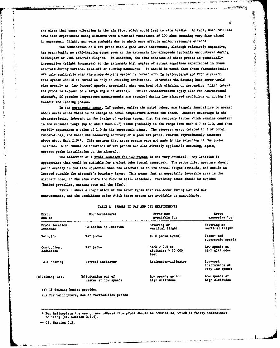
r 61the wires that cause vibration in the air flow, which could lead to wire breaks. In fact, such failures

have been experienced using elements with a nominal resistance of 100 ohms (meaning very fine wires)

in supersonic flight, and were probably due to shock wave effects and/or resonance effects.

The combination of a TAT probe with a good servo instrument, although relatively expensive,

has practically no self-heatinS error even at the extremely low airspeeds typically encountered during

helicopter or VTOL aircraft flights. In addition, the time constant of these probes is practically

insensitive (slight increases) to the extremely high angles of attack sometimes experienced in these

aircraft during vertical take-off or turning maneuvers. It should be noted that these characteristics

are only applicable when the probe deicing systen is turned off. In helicopters* and VTOL aircraft

this system should be turned on only in cruising conditions. Otherwise the deicing heat error would

rise greatly at low forward speeds, especially when combined with climbing or descending flight (where

the probe is exposed to a large angle of attack). Similar considerations apply also for conventional

aircraft, if precise temperature measurements are required during low airspeed conditions or during the

takeoff and landing phases.

In the supersonic range, TAT probes, unlike the pitot tubes, are largely insensitive to normal

shock waves since there is no change in total temperature across the shock. Another advantage is the

characteristic, inherent in the design of various types, that the recovery factor which remains constant

in the subsonic range (up to about Mach 0.7) rises gradually in the range from Mach 0.7 to 1.0, and then

rapidly approaches a value of 1.0 in the supersonic range. The recovery error (stated in Z of total

temperature), and hence the measuring accuracy of a good TAT probe, remains approximately constant

above about Mach 1.0**. This assumes that gross errors were not made in the selection of the probe

location. Wind tunnel calibrations of TAT probes are also directly applicable assuming, again,

correct probe installation on the aircraft.

The selection of a probe location for TAT probes is not very critical. Any location is

appropriate that would be suitable for a pitot tube (total pressure). The probe inlet aperture should

point exactly in the flow direction when the aircraft is in its normal flight attitude, and should be

located outside the aircraft's boundary layer. This means that an especially favorable area is the

aircraft nose, in the zone where the flow is still attached. Vorticity zones should be avoided

(behind propeller, antenna boom and the like).

Table 8 shows a compilation of the error types that can occur during OAT and CIT

measurements, and the conditions under which these errors are avoidable or unavoidable.

TABLE 8 ERRORS IN OAT AND CIT MEASUREMENTS

Error Countermeasures Error not Errordue to avoidable for excessive for

Probe location, Selection of location Hovering or Hovering orAttitude vertical flight vertical flight

Velocity TAT probe (Old probe types) Trans- andsupersonic speeds

Conduction, TAT probe Mach > 2.5 at Low speeds atRadiation altitudes > 60 000 high altitudes

feet

Self heating Servoad indicator Ratiometer-indicator Low-costinstruments atvery low speeds

(a)Deicing heat (b)Switching out of Low speeds and/or Low speeds atheater at low speeds high altitudes high altitudes

(a) If deicing heater provided

(b) For helicopters, use of reverse-flow probes

* For helicopters tle use of new reverse flow probe should be considered, which is fairly insensitive

to icing (cf. Section 2.1.5).

** Cf. Section 5.2.

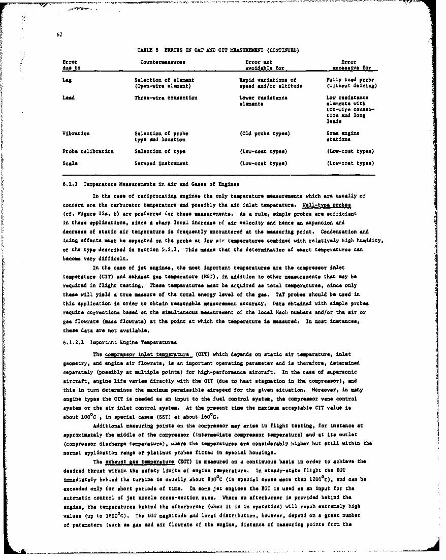
62

TABLE 8 ERRORS IN OAT AND CIT MEASUREMENT (CONTINUED)

Error Countermeasures Error not Errordue to avoidable for excessive for

Lag Selection of element Rapid variations of Fully iced probe(Open-wire element) speed and/or altitude (Without deicing)

Lesd Three-wire connection Lover resistance Low resistanceelements elements with

two-wire connec-tion and longleads

Vibration Selection of probe (old probe types) Some enginetype and location stations

Probe calibration Selection of type (Low-cost types) (Low-cost types)

Scale Servoed instrument (Low-cost types) (Low-cost types)

6.1.2 Temperature Measurements in Air and Gases of Engines

in the case of reciprocating engines the only temperature measurements which are usually of

concern are the carburetor temperature and possibly the air inlet temperature. Woll-type probes

(cf. Figure 12a, b) are preferred for these measurements. As a rule, simple probes are sufficient

in these applications, since a sharp local increase of air velocity end hence an expanoion and

decrease of static air temperature is frequently encountered at the measuring point. Condensation and

icing effects must be expected on the probe at low air temperatures combined with relatively high humidity,

of the type described in Section 5.2.1. This means that the determination of exact temperatures can

become very difficult.

in the case of jet engines, the most important temperatures are the compressor inlettemperature (CIT) and exhaust gas temperature (EGT), in addition to other measurements that may be

required in flight testing. These temperatures must be acquired as total temperatures, since only

these will yield a true measure of the total energy level of the gas. TAT probes should be used in

this application in order to obtain reasonable measurement accuracy. Data obtained with simple probes

require corrections based on the simultaneous measurement of the local Mach numbers and/or the air or

gas flowrate (mass flowrate) at the point at which the temperature is measured. In most instances,

these data are not available.

6.1.2.1 Important Engine Temperatures

The compressor inlet temperature (CIT) which depends on static air temperature, inlet

geometry, and engine air flowrate, is an important operating parameter and is therefore, determined

separately (possibly at multiple points) for high-performance aircraft. In the case of supersonic

aircraft, engine life varies directly with the CIT (due to heat stagnation in the compressor), and

this in turn determines the maximum permissible airspeed for the given situation. Moreover, in many

engine types the CIT is needed as an input to the fuel control system, the compressor vane control

system or the air inlet control system. At the present time the maximum acceptable CIT value is

about 100°C , in special cases (SST) at about 160°C.

Additional measuring points on the compressor may arise in flight testing, for instance at

approximately the middle of the compressor (intermediate compressor temperature) and at its outlet

(compressor discharge temperature), where the temperatures are considerably higher but still within the

normal application range of platinum probes fitted in special housings.

The exhaust &as temperature (EGT) is measured on a continuous basis in order to achieve the

desired thrust within the safety limits of engine temperature. In steady-state flight the EGT

immieditely behind the turbine is usually about 800 0 C (in special cases more than 1200 0 C), and can be

exceeded only for short periods of time. In some jet engines the EGT is used as an input for the

automatic control of jet nozzle cross-section area. Where an afterburner is provided behind the

engine, the temperatures behind the afterburner (when it is in operation) will reach extremely high

values (up to 1800 0 C). The EGT magnitude and local distribution, however, depend on a great number

of parameters (such as gas and air flowrate of the engine, distance of measuring points from the

63

afterburner plane, etc.) and can be evaluated only after taking all these effects into consideration.

Therefore, temperature measuring points behind afterburners are not customary in normal flying operations

but may become necessary in engine and flight testing.

6.1.2.2 Selection of Temperature Probes

The expected temperature ranges, the high flow velocity, and the available installation

possibilities must be taken into consideration when selecting the temperature probes for CIT measurements.

It was formerly the practice to employ thermocouples exclusively since, on the one hand, loes signifi-

cance was attributed to exact inlet temperature measurements and, on the other hand, thermocouples are

leos sensitive to vibration because of their small size and moreover, are relatively inexpensive. More

recently, however, special-purpose resistance probes have been developed that are insensitive to

vibration and yield a voltage change of about 4 mV/ 0 C at a resistance change of about 0.4 ohms per °C

temperature change and a current of about 10 mA, compared to about 0.011 to 0.045 mV/oC for thermo-

couples. Of course, this almost 100 fold increase in output voltage provides better resolution

and measuring accuracy. However, a much more important consideration is the noise voltage produced in

thermocouples due to intense engine vibrations which can be in the order of 100pV or more. This

phenomenon will impede the execution of measurements where high accuracy

is of paramount importance. The noise voltage is dependent on engine rpm (but is

not proportional to it) and has a frequency spectrum ranging from a few Hartz to several kUz

(Reference 54). Therefore, a special-purpose TAT probe with resistance element should be used in every

instan"e where the relatively low compressor inlet temperature, CIT, must be measured. Simple and

inexpensive resistance probes designed for minimum sensitivity to vibration are available for this

purpose. As examples, one design utilizes an open-wire nickel element (temperatures range from -70°Cto +260°C with a claimed accuracy of +0.1 ohm, corresponding to +0.1OC at temperatures near 100°C,

cf. Figure 20b), and another designed with a sealed platinum element (temperature range from -260 to

+600oC, cf. Figure 20a). Special configurations of these probes are especially suited for measurements

in the compressor (intermediate compressor temperature) and behind the compressor (compressor discharge

temperature). Special-purpose types are available for combined pitot-static pressure and inlet

temperature measurements where the probe must be able to sustain mechanical damage without shedding

parts upon deformation*; some of these can be protected against icing with the aid of bleed air. An

important consideration for the selection of a probe is the problem of the tine constant, since

electronic fuel control systems require a much shorter probe time constant than hydromachanical fuel

control systems where excessively short time constants would result in unpleasant control oscillations,

especially in the vertical lift engines of VTOL aircraft.

On the other hand, thermocouples are the only recommended probe type for exhaust sas

temperature measurements, since almost all presently available resistance probes would suffer damage

at this location during the short-time temperature peaks that develop frequently at this point. TAT

probes with exposed elements are shown in Figure 39. The exposed and shielded configurations of simple

probes shown in Figure 38 are not as desirable since their recovery factor is flow-dependent. The

computation of corrections for different states of operation becomes very complicated. The Imnersion

depth L of thermocouples into the gas flow should be about 12 to 15 times the diameter of the

cylindrical part of the probe, in order to keep the radiation error at a low level. Also refer to

Section 5.2.2 and Figure 73.

In the case of exhaust Sas temperature measurements behind afterburnerswe must taka into

consideration that the maximum temperatures experienced by the probe greatly exceed the temperature

range for which the calibration of most thermocouples is stable. Therefore, their life will be short,

even in the case of special-purpose types, and the probe must be recalibrated at the maximum permissible

temperature (to avoid destruction of the element) after every flight or series of measuremants. It is

unknown whether probes of tungsten rhenium are available for applications in aircraft. This material,

which is used in space technology, permits the measurement of temperatures up to 3100 C with a measuring

uncertainty of about +7°C.

SDanger of engine damage,

64

6.1.2.3 Selection of Probe Locations

The cross-sections Just ahead of the compressor and just behind the turbine have proved to be

£004 probe locations for CIT and EGT. It is much more difficult to determine the number and arrangementof probes at the selected station. Radial velocity and temperature gradients occur in air or other

gases moved at high velocity through a duct, depending on the types of flow that develop, but these do

not differ excessively since air and other games have a Prandtl number close to 0.7. It is quite

difficult to determine the temperature gradients in the flow through computation, since inlet and exhaust

ducts deviate greatly from the "ideal" cylinder with respect to their length and geometry, and the

instantaneous or effective values of too many parameters would have to be included. M oreover. the

a' engine stations where temperatures are usually measured are located at the transition points between thecircular cross-section. of inlet and exhaust ducts and the annular flow cross-sections of compressor

and turbine. The conditions prevailing in the air inlet of a supersonic jet were already described in

F Section 5.2.2 and illustrated in Figure 65. Therefore, the frequently used procedure is to measure

the radial velocity distribution first, (possibly as a function of sanle) using pitot tubes (or a

"comb array"), in order to obtain an idea of the temperature distribution to be expected.

When it is found that there will be no asymmetrical pressure or temperature distributions

over the entire operating range of the engine, it is theoretically sufficient to use a single probe

per cross-section where the temperature is measured. If the pressure distribution is asymmetrical ,at

least four to eight probes must be provided in different sectors. The conventional, fixed array is

one to four resistance probes in front of the compressor,* and four to twelve thermocouples behind the

turbine. The latter are frequently designed as dual yrobas (with two elements). One set of these

elements is switched parallel for an average temperature measurement, while the other elements are

each individually connected to a test plug in order to measure, for instance, the temperature behind

each individual combustion chamber.* For flight testing purposes,* considerably more probes are

usually provided in front of the compressor, in order to monitor the temperature distribution over

the cross-section.

The exact location of the probes in the cross-section to be measured must be selected so

that the temperature-sensitive elements are placed neither too near the tube or engine side, nor

exactly in the center of the flow, since it is the mean value of temperature that is desired. A"rule of thumb" is to place the probe in the zone between 25% and 75Z of the radius in the case of

a circular cross-section, or into the zones between about 12% and 362 and/or 64% and 882 of the

ring width in the case of Annular cross-sections. Several concentric rings of probes with separate

outputs are always required where it is intended to acquire not only the temperature relationships

during flight but also the conditions prevailing during start-up of a cold engine. This is the only

possible method to acquire the distribution of the temperatures that are entirely different in this

state of operation (or to acquire the temperature differentials between tube wall and the gas), in

order to form conclusions as to the most advantageous probe location for the acquisition of the mean

temperature. Also, conditions in the air inlet of vertical lift engines in VTOL aircraft are

especially critical. An inhomogeneous air mixture of continuously changing temperatures

and different temperature distribution over the cross-section area is encountered at these inlets

due to exhaust gas reflection off the ground and recirculation, together with the colder external air.

A typical probe array in the inlet of vertical lift engines, using the resistance probes

shown in Figure 21, was presented in Figure 66, where the array parallel to the flow (a) is the better

solution. In order to determine the mean temperature directly, a possible array places three probes

in series and three such groups in parallel so that the resultant total resistance will be equal to

the resistance of a single probe. Another possibility is to place four probes (each with a nominal

resistance of 50 ohms) in series, and to place two of these groups in parallel so that a total

resistance of 100 ohms will result. In that case a mass-roduced instrument (for 100-ohm probes)

can be used.

6.1.3 Temperature Measurements in Liquids

As a rule, measuring the temperature of liquids in containers does not involve any

difficulties since the flow velocities are low and the temperature changes very slowly. The probe

must not be installed on the topside but on a side wall or on the bottom of the container. If It is

installed on a side wall the location must be low enough so that it will always be wetted by liquid

65

as the level in the container drops. If It is installed on the container bottom, and if there isa

possibility of a sediment forming, the probe must be long enough to pass through the sediment (cf.

Figure 92) without penetrating the surface of the liquid. In all instances it must be kept in mind

that the imersion depth of the probe (which generally will be of the well-type) should not be less

than six to eight times the diameter, in order to keep the heat conduction error small. Also, "dead

spots", i.e., areas where there is no flow, should be avoided since liquid layers of different

temperatures may form these locations. For the same reason, the indication can vary In aircraft on the

ground, for instance when wind gusts set the liquid into slow motion.

Where temperatures of liquids are measured in tubina it must be kept in mind that the

Prandtl number of liquids differs greatly from one, so that the velocity and temperature distribution

over the cross-section area differ greatly. If -he Prandtl number is very high (for instance in

lubricating oil) the liquid temperature will be uniform over moat of the tube cross-section and will

show a high temperature gradient only Ieadiately adjacent to the tube walloif the wall and liquid

temperatures differ greatly as a result of heat conduction or radiation. A good compromise for the

liquids used in aircraft (as it is for air) is to place the temperature probe outside the tube axis

(in the zone from 0.25 to 0.75 r).

Figure 93a shows how relatively long probes cam be accommodated in a bend of a liquid

line. Care must be taken that the flow encounters the temperature-sensitive part of the probe first

and the base last, since the latter will have essentially assumed the temperature of the tube wall.

Also, the line can be insulated externally to reduce the conduction error (unless the line is

extremely short), so that the tube will approximately assums the temperature of the liquid. Possibly

the use of appropriately designed struts may be worthwhile (Figure 93c ) which increase the distance

betweca threaded socket and tubeland also permit the employment of relatively large probes in very

narrow tube cross-sections. For special applications, i.e., for lines with relatively high internal

flow velocity, cylindrical probes for installation in tubing are available (Reference 25). Another

frequently used procedure is to measure the temperature indirectly thtough the tube wall (cf. the

next Section).

The usual temperature sensors are well-type resistance bulbs, usually with a nickel element,

of the type illustrated in Figures 12a and b. Where these are combined with inexpensive indicating

instrument& that require a very large measuring current, a self-heating error must be expected. This

error is greatly dependent on. flow velocity so that the indication nay require appropriate correction.

6.1.4 Temperature Measurements on Surfaces and Solids

The measurement of surface temperatures on aircraft is often very difficult. Some of

the factors to be considered in the design of an installation include: (a) the installation of a

temperature sensor with leads always causes a disturbance of the surface tomperaturexb) aerodynamic

conditions prohibit the use of some probe locations which otherwise nay appear to be desirable;

and (c) measuring the internal temperature of solid bodies requires special bores that may adverselyaffect the strength of the body in question.

Particular care muut be exercised in the design of the probe installation In order to obtainthe best heat transfer possible between surface and temperature probe. This is done using large-area

screwed, soldered, or welded contacts as shown in Figure 94, or by the extremely sparing use of an

adhesive of good heat conduction characteristics. In short, there must not be any air, paint or oxide

layer, etc., that would provide thermal insulation, nor should it be possible for such a layer to form

after probe installation. Especially good conditions exist where a recess can be drilled or machined

into the surface in order to embed the temperature probe flush with the remaining surface (Figuze 94g)

This will avoid any major perturbance of the boundary layer even on surfaces with a high-velocity inflow

(such as aircraft skin). The emissivity of the probe surface should be matched with that of the

surface to be measured (for instance through blackening, surface treatment, and the like) especially

where measurements are performed in rarefied gases (high altitudes). This avoids any perturbance

of the temperature equilibrium as a result of differences in radiation. Of course, the thermal

capacity (and hence the volume) of the temperature probe should be kept as small as possible compared

to that of the surface to be measured so chat the probe will follow any temperature change rapidly.

Yet the presence of the probe can disturb the temperature field considerably due to heat conduction

along the electrical leads as seen from the profile of the isotherm. in Figure 95a. The type of lead

co0nfiguration ilustratd should also be avoided because of the danger of a lead breaking at the element.

heat conduction to the surface, end the minimum length L should be about 50 times the eadaetrd.For measurements on the outside of the aircraft skin the leads are best placed parallel to the air flowuntil they reach the nearest frame, stringer, or web, to reduce the perturbation of the flow; from therethey are passed Inside the aircraft, unless it is possible to measure the temperature indirectly asdescribed below. Unfortunately, it is rarely possible to place the leads parallel to isotherms on theoutside of the skin, as It is seen from the examples of surface temperatures shown in Figures 97 and 98.

In the case of direct surface temperature measurements the actual temperature on the outside(for instance, of an item of equipment or a pipe) is measured by placing a temperature probe on theoutside. However, if the probe and its imediate vicinity are covered by an insulating layer, atemperature will be measurad that is very close to t'.at of the opposite side of a metal skin. This

L will permit indirect surface temperature measurements, i.e., a measurement of the surface temperatureof the aircraft skin in an air flow by means of a probe installed on the inide of the skin (cf.Figure 95c).* The measured value would be too small unlessn sufficient insulation were placed over theprobe location. However, if this insulating layer were to extend over too large an area the reducedloss of heat would excessively change the conditions compared to the normal state, and the measuredtemperature would be too high. Consequently, most of the heat conduction error caused by the leads ofthe temperature probe can be compensated via the area end thickness of this insulating layer*.

A very popular procedure is the indirect temperature measurement of a liquid flowing througha pipe, measuring from the outside of the pipe. Figures 96a through 96c show the temperature

relationships in the event of unfavorable heat conduction by the leads, the conditions where the leadsclose to the probe are placed properly parallel to the pipe, and the relationships prevailing when anadditional insulation is wrapped around pipe end probe. It is seen that in the latter case the

temperatures of liquid end outside tube wall (and the probe) are almost equal. However, this applies

only where the length of the pipe is at least 20 times the pipe diameter, and where the probe islocated at an adequate distance from the ends of the pipe. In other words, the pipe must be able to

assume the temperature of the liquid. Short and thick-walled tubing located on large aircraft elements

will tend to assume the temperature of that element (engine and the like) and are, therefore, unsuited

for this measuring technique.

Similar considerations apply for temperature measurements in solid bodies, where themeasurements must take place with a minimum perturbation to local temperature relationships. Where thegeometry of the body permits, the bore for the temperature probe should be as narrow and deep aspossible, and the ratio of bore depth to diameter should be greater than five to one where the bodyhas good heat conductivity, and greater than about 15 to 1 where it has poor heat conductivity. If theelectrical leads are placed along an isotherm on the body and can be secured to the body with good heatconductivity, the heat removed from the leads (heat conduction error) will not be removed from the probe

location but from the environment in which the leads are embedded.

Both resistance elements and thermocouples (for higher temperatures) are used as temperatureprobes. Figure 94 shows some typical resistance probes for surface temperature measurements, and the

mounting technique. Figure 23 shows resistance probes for measurements in solid bodies a tip-sensitive

well-type probes in Figures 23a and b, and a special design with a spring-loaded element for cylinder

head temperature measurements in Figure 23c which can be exchanged at any time for the thermocouple shownin Figure 41a (provided that the leads and the indicating instrument are switched, too). Figure 41

also shows additional probes with thermocouples, including probes screwed to pipes, screwed under spark

plugs or bolt heads, and blind rivet probes. Finally, Figure 95 shows a very small thermocouple that can

be made from thermocouple materials (for instance AN4 30 wires or from a thermocoaxial line) and is

economical especially when made in large numbers. The twisted end of the lead is spot-welded to the

aircraft skin. Where the surfaces or bodies have poor heat conductivity the thermocontact is welded to

a metal plate which is then attached to the body with the best heat conductance possible. Where thetemperature of solid bodies is measured, this array must be embedded into the body. It must be kept inmind that newly made thermocouples should be aged prior to use by glowing them several times, since

*This can be determined through comparison with a contact thermometer, making sure that the conditionsare as similar as possible to normal measuring conditions.

67

otherwise the calibration will change too rapidly. The use of series connected thermocouples

for obtaining measurements of mean temperature is not possible, if the thermocouples are grounded.

Incidentally, special resistance probes with extremely emall temperature lag errors are

available for measuring temperatures on surfaces with rapidly changing temperatures (for instance,

fuselage skin of %UTOL aircraft in the take-off or landing phase). This is achieved through a special

array of different resistances in the same element, using a balancing circuit: "Compu-Therm" principle,

References 86 and 87. Special thermocouple types are available for measuring the heat flux (the

so-called "heat flux" transducers, References 92 and 93), whose description would exceed the scope of

this paper.

Additional information on surface temperature probes, the associated adhesives, and the like,

can be obtained from the appropriate company literature.

Temperature-sensitive paints shall be mentioned here that are applied to the surface of the

body in question and will show a color change when a certain temperature is exceeded, permitting the

indication of temperatures in the range between about 370 and 670 C. These so-called "thermocolors" are

supplied in the form of powder that is suspended in denatured alcohol and thinly applied with brush

or spray gun. The drying time is about 30 minutes. The temperatures must prevail for a period

of 30 minutes in order for the full color change to take place. If the tine is only 5 seconds, the

indicated temperature will be about 10 to 40Z lower than the actual temperature. The color change will

be retained for a certain period of time if the surface cools slowly*. The original color will be

restored when the surface is wet. These colors can be used several times. Also, there are types with

multiple color change (for instance, initial color pink, changing to light blue at 650 C, to yellow at

145aC, to black at 174aC, and to olive drab at 340CC). A similar behavior is characteristic for

"Detectotemp paints" and "Thermochrome crayons"; however, the former -cannot be used in the open air,

i.e. on the outside of an aircraft skin (Reference 96). The Thermochrome crayon must be applied to a

hot body, otherwise the color change will take place too early. If the body is above the temperature

for which the paint was selected, the color change will take place immediately. Temperature indicators

in the form of self-adhesive ribbons are especially well-suited for monitoring purposes, i.e.,for long

term observations to determine whether a certain temperature has been exceeded. Different types of

the so-called "tamp-plates" (Reference 95) are available that provide from one to eight calibrated

color points which assume a black color permanently when the indicated temperature is exceeded.

Finally, there are mechanical temperature indicators, for instance the so-called "templugs". IThese resemble grub screws (about 5 mm long, 2.5 = diameter) which are screwed into appropriate bores

in the object whose temperature is to be measured (for instance, a turbine housing). The hardnass of

these indicators will change as a function of temperature and exposure period. The templug is subjected

to a hardness test in the laboratory after completion of the test in question which permits subsequent

temperature determination with an accuracy of +50 (Reference 13). Another comparable technique hasrecently been reported which utilizes capsules filled with diamond powder that has been exposed toradiation in a nuclear reactor. The change in the density of the powder is proportional to the tempera-

ture reached, and is subsequently determined through X-ray photography with an accuracy alleged to be±3 0 (Reference 102).

6.2 Selection of Thermometers

The aspects which are important in the selection of a thermometer include:

Type of medium to be measured: ambient air, engine exhaust gas, fuel, aircraft

skin, equipment, etc.

Temperature range to be covered.

Measuring purpose: permanent installation or test rig.

Type of aircraft: airspeed range, space and weight considerations, etc.

Type of measurement: individual, multiple, mean value, differential, or temperature rate

measurement; point or area measurement.

Type of data acquisition: instrument reading, telemetry, airborne recording, or combinations

of these techniques.

* Exercise caution in the treatment of objects that are exposed to an air or gas flow!

68

Combination with other airborne systems such as air data computers, engine control

t systems; interfaces required for this purpose.

Required meaauring accuracy, indication resolution, recording accuracy, Measuring

duration and sampling cycles in the case of intermittent measurements.

Required response: time or local resolution as a function of airspeed.Available equipment and modules.Available funding.

Price and availability of the required equipment.

Available capabilitie&' for in-house fabrication.

Available calibration and testing facilities.

Type of data acquisition and data processing.

Requirements Imposed on the measured data by other users.

Available time for preparations.

After considering these points the design type of the thermometer to be used is determined

first: resistance thermometer. thermoelectric thermometer, temperature-sensitive paint, and so on.

Since* electrical thermometers are used in the majority of cases, the advantages of the two types @hall

be compared again at this point:

Advantases of the resistance thermometer:

Greater sensitivity to small temperature changes, resulting in a much greater output voltage.

Loes complicated and inexpensive equipment for indication, recording, or signal processing

for telemetry purposes.

Greater accuracy end stability (up to 30 times better over limited temperature ranges).

Failures (short circuit or breakage) are easier to discover.

Less sensitivity to noise voltages (resulting from engine vibration), parasitic thermo-

voltages, end the like.

The leads weigh less and are cheaper then compensating lines; longer leads are possible

for high-resistance probes.

The output voltage per degree of temperature change can be varied within broad limits

through appropriate design of bridge and supply voltage, and it is easy to set up computing

bridges. (However, doubling the bridge and supply voltage will result in four tines the

self-heating error of the probe!).

A temperature reference point or compensating device is not required.

Probes with close tolerances can be supplied so that recalibration is not necessary when

probes are exchanged.

on the other hand, thermometers using thermocouples have the following advantages:

The temperature range that can be covered is greater.

An external current source is not required if directly indicating instruments are used.

Thermocouples for many applications can be made in-house at low cost.

Thermocouples have greater stability than resistance elements at high temperatures.

Consequently, these two types supplement each other, the resistance thermometer having a clear

advantage in the temperature range from about -1O00 to +250 0C in most instances, while only the thermo-

couple has the necessary characteristics in the range from about +7000 to 1500 aC*.

Having decided on a certain thermometer type it is necessary to select the probe and the

indicating or interface system for telemetry or recording facilities, in accordancs with the

considerations outlined above. Where it is necessary to use some equipment that is already available,

consideration must be given to the fact that the system can be no better then the (component which

contributes most to the measurement error. The cases of errors named in Section 5.2 must be considered

when new equipment is prozured. This means, for instance, that in the case of a resistance thermometer

*Tungsten - Rhenium. thermocouple up to +3100 aC.

69

the probe with the highest possible resistance must be meted to an instrument that will not cause

excessive self-heating in the probe. Moreover, manufacturer's information must be critically examined

to fully understand its applicability to the measurement requirements for which the component has been

or will be procured. Caution is indicated in the case of companies that are very sparing with data and

documentation or cannot state the test conditions under which a certain characteristic (such as self-

heating) was measured*. This type of advertising may be indicative of an effort on the part of the

contractor to expand into new areas, such as sensors, indicating instruments, and the like ,withoutspecialized knowhow and suitable test equipment, nor even am in-house development activity that perf orms

measurements in aircraft itself. "Cheap" products can turn out to be very "expensive" when the

measurements are finally obtained.

In this connection we must also discuss the in-house fabrication of probes, bridge circuits,

and the like. This used to be a common practice since, among other reasons, suitable signal conditioners

and indicating instruments with recording outputs were not commercially available. The most frequent

shortcomings of this class of equipment are: unacceptably high self-heating of the probe as a result of

improper dimensioning of the bridge circuit, the temperature dependence of the dc amplifiers used,

inadequately stabilized supply voltages, and the like (cf. Section 2.2 and 3.3). It is recommended

therefore that modern servoed instruments with independent measuring outputs (potentiometer, encoder,

aet.) be employed in every instance where exact temperature measurements in air and other gases are

required. In-house development of comparable equipment requires years of specialized experience and

iii time-consuming and, therefore, in most cases more expensive.

Prior to the acquisition of probes, signal conditioners, and the like, consideration should

be given to the cost effectiveness of procuring expensive components, with more stringent specifications,

in the interest of lowering the cost of other operations. As an examplesone would expect that in a

better system, the number and complexity of the corrections required would be reduced, and this in turn

should lower the uost of post flight operations. In addit 'on, the results should be more accurate and

easier to evaluate. (cf. Section 6.4)

6.3 Calibration of Thermometers

The characteristics of the thermometer and all the associated recording and/ol indicating

devices must be known before any accurate temperature measurements can be made. This means that all

errors must be identified and defined for ell flying states that are of interest. Measures required

for this purpose can be subdivided into three stages:

(a) Error determination on individual components in the laboratory.

(b) Error determination of the entire thermometer after installation in the aircraft.

(c) Error determination while airborne.I

As a result of the interdependence of many errors and the influence of many parameters that

are difficult to evaluate, all experiments and measurements must be planned and excecuted so that the

errors are acquired individually wherever possible. The measured data must be available in a form

that can be evaluated directly, for instance, as a function of Mach number and altitude, so that

tine-consuming conversion routines will be eliminated.

Test facilities available to instrument engineers during flight programs are normally rather

limited. Therefore, the following discussion neglects those measurements that would require special

facilities such as wind tunnels, etc. However, decade resistance boxes, temperature calibration baths

with precision thermometers, digital multimeters, and a temperature test chamber with a range from,

for instance, -8 to +800C (but at least from -20 0 to +80 0C) must be available. A thermocouple

thermometer tester, a small electric furnace and a "Jetcal analyzer" with all accessories should be

available for testing thermocouples.

6.3.1 Calibrations in the Laboratory

As a rule, only the following activity can take place in the typical laboratory or test shop:

*This applies also to information such as "recovery factor *1.0", "self-heating so small that it canbe disregarded", etc.

"70

(a) Measurements of Resistance Probes

The probe calibration error EcAL is determined for the temperature range of interest in a

calibration bath agitated at constant rate, by comparing the acquired resistance values to the appropriatetable of standard valuse (for platinum, nickel, etc.) and to the liquid temperature determined with a

precision thermometer. Although the self-heating effect is much smaller in lquide than in air, the

probe should be operated at the smallest measuring current possible (for instance, 1 mA for Ni and Pt

probes, and about 0.1 mA for thermistors), in order to be certain that the self-heating error will

remain below a level of 0.10C.Additional measurements can be performed in the laboratory on resistance probes used to measure

temperatures in- aguid. The prerequisite is that the same liquid be used that will be measured by the

probe installed in the aircraft ard that the liquid flow velocity be the same as prevailing at theintended probe location. The heat conduction error Ec can be determined, for instance, by completely

Immersing the temperature-seasitive part of the probe in an agitated liquid bath at, for instance,

+10e0 C, and packing the head of the probe in ice. The difference between the measured temperature and

the temperature of the liquid will yield the heat conduction error for a temperature difference of

1000C between liquid and probe head. Repetition of this test at several lower temperatures (such as

80°C, 60°C, 400 C, 200C and 10°C) is advisable because the heac conduction error is a non-linaarfunction of the temperature differential. Detailed instructions for determining the heat conduction

error are provided in Reference 25.

The temperature las error EL can be determined by rapidly alternating the probe between two

agitated baths of different temperatures, measuring the time required to indicate 20%, 50%, 63.2% and

90% of the temperature difference (cf. Section 5.2.3).

The self-heating error R2 can be determined for a givan type of liquid and liquid velocity

at a desired temperature provided the resistance of the probe is first measured with no significant

self-heating (using, for example 1 mA for Ni and Pt probes, and 0.1 a& for thermistors). The currentis then increased to ten times the initial value or more. A milliammeter is placed in series withthe probe, and an electronic millivoltmeter of very high input resistance is placed in parallel.

Assuming the temperature increase was 1.500 C and took place at a current of 10 mA and a voltage of 5.00 V,i.e. at a power of 50 MWI the self-heating effect wrill be 1,500C/50 %W, or 0,03°C/mW. Data obtained

for a given liquid and a given liquid velocity are almost impossible to extrapolate to other liquids

(or gases) at the same or different velocities, since they are also dependent on the probe design end

will yield different factori for each probe type,

A rough estimate applicable to certain well-type probes is that the time constant can beabout 30 times greater in air, about 2 tines in oil, and about 1.5 times grester in liquid oxygen

than in wvtart under otherwise equal conditions the self-heating effect in °C/mW can be about 100 timesgreater in air, and about 2 times reaster in oil and in liquid oxygen than in water, provided aliquid velocity of 5 ft/sec is assumed in every instance. The actual values of other probe types can

deviate quite considerably from these relationships.

The calibration of probes for surface and solid body temperatures can be acquired in liquid

baths, too; however, measurements of self-heating, temperature lag, or heat conduction are meaninglessif performed on individual probes before they are installed, and in most caeesdifficult to obtain when

the probes are installed on the solid body.

In the case of probes for air and see temperature measurements little more than the calibrationerror can be determined in the laboratory. All other errors must be determined in the aircraft (unless

suitable wind tunnels are available), since they are dependent on flight conditions (cf. below).

(b) Measurements of Thermocouples

This discussion of the measurement of thermocouple characteristics will be confined to the

determination of the probe calibration error E CAL In using furnaces special care must be taken to

assume that the immersion depth is adequate and that attention is given to any effects caused by the

high temperature gradient in the region where the leads are passed through the furnace wall (cf.

Section 3).Calibrations using the "Jetcal analyser", which is discussed below, may prove to be

considerably better. A detailed description of the calibration of thermocouples is found inReferences 13 and 42.

71

(c) Calibration of Instruments, Signal Conditioners, etc.

The following information on the measurement of instrument characteristics also applies to

signal conditimners, telemetry, and recording apparatus. It should be mentioned at this point that

theae devices, unlike the usual practice with probes, are not always supplied in aged condition,

Therefore, it is advisable to operate new equipment for an uninterrupted -ariod oi 24 hours, if

possible at an increased ambient tonr -ture, before proceeding with its calibration*.

Laboratory tests that can be performed on this equipment include the following:

(a) The instrument scale error ESC, at room temperature (approx. +20°C) and with the specified

lead resiotance, can be determined by substitution of a precision decade resistance box

for the probe**. A warm-up period of at least 30 minutes must be allowed before this

measurr is made.

(b) Simulate a step change in the temperature at the probe by switching between two resistances

that correspond to the probe resistances at the lower and upper limit of the measuring

range, to determine the lan of the instrument (or the follow-up time in the care of

servoed instrurwnts).

(c) SIt -late ve-,, small temperature changes at the probe by introducing very small changes in

the co~ected resistance to determine the resolution of the instrument. Repeat this

test while lightly striking the instrument to determine the effect of friction inside the

inst .ument.

(d) Turn the equipment off for a period of not less than 30 minutes (unti. the instrument has

returned to room temperature), and measuce the time required to achieve a constant

indication for three different inputs, perhaps 30%, 701, and 1002 of full scale, to

determine the warm-up time. Let the instrument cool down between each of the three

measurements.

Re) Repeat the measurements described under item (d), above, at -20 0 C and then at +60 C, r.terplacino the instrument in a temparature-controlled chamber***. Leave the resistance box

outside. These tests can be used to determine both the maximum warm-up time that must be

all3wed before measurements can begin, and particularly the instrument temperature error.

This error is not normally specified, rather, the errors are determined for a constant

input at the lowest, intermediate, and highest temperature for which the instrument

is designed. These are combined and presented as a mean scale error so that this error

appears as a systematic error with a certain dispersion range (cf. Section 6.4.1).

(f) If all components, i.e., the actual wiring, plugs, circuit breakers, etc. are available

prior to installation in the aircraft, t is also possibli to determine the el3ctric lead

erro..r E,, This error is variable, depending on the indicated temperature, especially

in the case of simple instruments. More details are provided in the following chapter.

6.3.2 Flight Line Calibrations

Unlike the individual measurements in the laboratory that were discussed in the preceding

mection, the thermometer system as a whole can be tested "in situ" on the flight line.

(a) Resistance 'Werometers

The final calibration of the total thermometer system can be performed by replacing the probe

with a derads resistance hox. In this procedure, the following comments may prove helpful. Care should

4e taken to use connections which are as short as possible and which are made using AN16 gauge wire,

ur larger****. This precaution will help avoid introducing additional electrical lead errors. In

• Tý was foumd in the case of certain types of servoed equipment that this break-in period reduced the iwarm-up time from 40 minutes to 8 minutes.

• Its loasing capacity should be greater than 1 wcct, if possible, to avoid self heating of the resistances

*** These values depend on the ambient temperaturas the instrument is expected to experience in the aircraft.

A*** If the probes have very low resistance, the resistance of these lines must be deducted from the valueof the decade reslitance.

72 •

selecting resistance box values, if the actual probe calibration is used in lieu of a standard calibra-

tion curve, then probe replacement will require a re-calibration.* This procedure willhowever, reduce

the corrections necessary when the raw data are processed. As an example, some indicators are equipped

with externally-accessible trim pots which are used for line compensation and/or scale adjustments.

When these are properly adjusted, the values of indicated temperature are as close to the corresponding

values of actual temperature as the probe and indicator calibration anomalies will allow. This combined

correction may not be suitable over the full range of the scale, because, for example, of different

n•n-linearitiea in the calibrations of the probe and indicator. In this event, a decision must be made

regarding the maximum allowable deviations between indicated and actual values over the portion(s) of

the scale which are of prime interest. This procedure is illustrative of the steps that can be taken

in setting up a system to facilitate the evaluation of the data acquired during test runs. Ideally, in

r: this instance, for example, the only additional errors that would have to be accounted for would be those

dependent on the flow velocity.

In the case of thermometers used for ambient temperature or compressor inlet

temperature measurements(OAT or CIT measurements), additional testing on the flight

line is hardly possible, except for functional tests in which case the probe deicing heater must be

turned off. On the ground, the indicatinn will almost always deviate by some amount from the static

air temperature, partly because the time constants in this state are very long, perhaps 15 minutes and

more. If the probe heating system (deicer) were turned on, the temperature indication would rise to

more than 100 C, and in probes with open-wire elements it is likely that the element would be damaged.V.t A functional test, in addition to the calibration described above, can be performed on

thermometers for measurements in liquids, on surfaces**, and in solid bodies.** In some cases, the

engines must be running for this functional test in order to simulate flight conditions. Also,

comparison measurements might be taken in this state in order to determine the effects of self-heating

or heat conduction errors. Many inexpensive thermometers designed for measurements in liquids allow for

the self-heatinS error of the probe in the calibration of the instrument. In that case, the scale

calibration will apply only for the liquid in question and for a certain velocity of the liquid flow.

When the engines are turned off, the indication will fluctuate and become unreliable, especially whenii ~natural convection satv in, because the probe is subject to appreciable self-heating. A number of good •

thermometer testers are ailable, but the operating instructions which are provided do not always

adequately discuss all potential sources of error (especially self-heating).

(b) Thermometers with Thermocouples

The most important application for thermometers of this type is in the measurement of the engine Iexhaust gas temperature (ECT). In this case, it should be possible to simulate most of the operating

conditions existina in flight by running the engines on the ground. However, the determination of the

actual measuring accuracy of thermometer arrays in an engiite is very difficult under these conditions.

A good aid in this case is the so-called "Jetcal analyzer" or comparable apparatus. This set

permits, among other procedures, a functional test of the entire EGT system with non-running engines,

testing each ýhermoelement and the whole array for continuity, short circuits, etc. Generally, the entire

LGT system can be terted w'ith an accuracy of about +40 C. The different capabilities of the set can be

wien from the operating manual supplied with it.

6.3.3 In-Flight Error Calibration

6.3.3.1 General

In the majority of temnj.ature measurements, e.g., in liquids and solids, in-flight error

evaluation is confined to a check against the results obtained in the laboratory and on the flight line,

and/or to the determination of that probe location which will result in the minimum position error.

Optimum probe locations can only be determined in-flight since these conditions cannot be adequately

simulated on the ground. The procedure generally used involves the installation of thermometers st

different locations to measure the same parameters. The outputs are read out either individually or

* This does not hold for nrobes with close tolerances.

** Provided the air flow about the aircraft that exists in flight does not play any decisive r.ole.

73

comatated onto a eingle channel and read sequentially. The probe that shows the least position erroris used in Succeeding flights.

The determination of the position error of probes for OAT and CIT measurementa using in-flight

technique.- %a, at time. justifiable because the resulting flow, pressure, and temperature relationships

at the probe or at the measuring element can be created only in flight. Since position errors are

dependent an altitude and airspeed or Kach number, the errors in the aircraft's pitot-etatic system

muet first be determined In special instrumentation flights. Techniques for obtaining these calibre-

tions are described in the conventional flight test manuals. However, if a reference thermometer that

could be used as a "standard" (cf. below) Is not available, then only those procedures wherein the

static air temperature is determined by a thermometer on the ground or by a radio sonde at flight

altitude can be used. To perform thermometer calibration runs at different airspeeds and the same pressure

altitude, or correlate calibration measurements obtained in different flights and in different flight

regimes, it is very Important that accurate measurements of the static pressure position error as a

functIn of airspeed are available. In the presence of unfavorable meteorological stratification in

the troposphere, even small deviations from equal pressure altitude can result in large changes of

static air temperature. The differences between the true Kach number and the indicated Mach number

(which is subject to pressure errors) as a rule have a minor effect on the accuracy of error determine-

tion. However, they cannot be disregarded, especially in the near-sonic airspeed range, since the

pressure error in this flight range can assume respectable magnitudes. Figure 99 shows the effect of

a relative error of LM/M s 1Z on the determination of static temperature as an absolute magnitude and

as a relative temperature error.

All calibration flights to determine the pressure and temperature error of sensors on the

aircraft should be carried out with due attention to suitable meteorolosical conditions. This will pay

off in terms of less dispersion of measuring errors. Instrumentation programs of this type can be

accomplished quicker at test sites having favorable climatic conditions.

The evaluation of weather situations is based primarily on the vertical temperature

stratification and, secondarily, on the vertical structure of the winds. The data required for this

evaluation are supplied by the radio sonde stations of the national weather service located in or about

the test area; these are acquired at the standardized world-wide times at 00.00 GMT and 12.00 GMT.

Where this information turns out to be inadequate, special radio sonde or aircraft missions must be

accomplished to determine the temperature as a function of pressure altitude.

In any event tt is better to determine the meteorological stratification beforehand, and

then carry out the instrumentation flights in the suitable strata, rather than perform the

instrumentation flights at preplanned altitudes without meteorological information. The risk

inherent in the latter approach is having to discard the data because of excessive meteorological

errors which, of course, can render the data useless for error determination.

The following types of vertical stratification are suitable for the determination of

pressure and temperature measuring errors under in-flight conditions:

(a) Temperature structure: Attempts should be made to locate areas where the ieothermic

vertical stratification, i.e., the vertical temperature gradient, is 0C/lO1m, or as close as possible

to this value. Measurements should never be performed at gradients in excess of -1 0C/l00 m (dry adiabatic

temperature gradient) or +10 C/lOOm (inversion). In the presence of stratification of this magnitude,

an altitude change of +1Om (±30 ft) will cause a temperature change of 0.2 0 C, which is in the order of

measurable errors. It requires special skill on the part of the pilot to maintain altitude with an

accuracy of this order, especially where steady flight conditions must be established at relatively

high airspeeds.

Thermoconvective weather situations are unsuitable. These are situations with vertical

interchange caused either by radiation via a heat increase of the ground (boundary or exchange layers)

or by a mixture of air masses of different energy levels. Periods of minimum exchange are favorable

for measurements, especially at low altitude. These are the periods where the direction of radiation is

changing, as well as all weather situations with denne cloud stratification and no convection phenomena.

Moreover, there must not be any precipitation, unless it is intended specifically to test

the effect of the liquid water phase on the airspeed error.

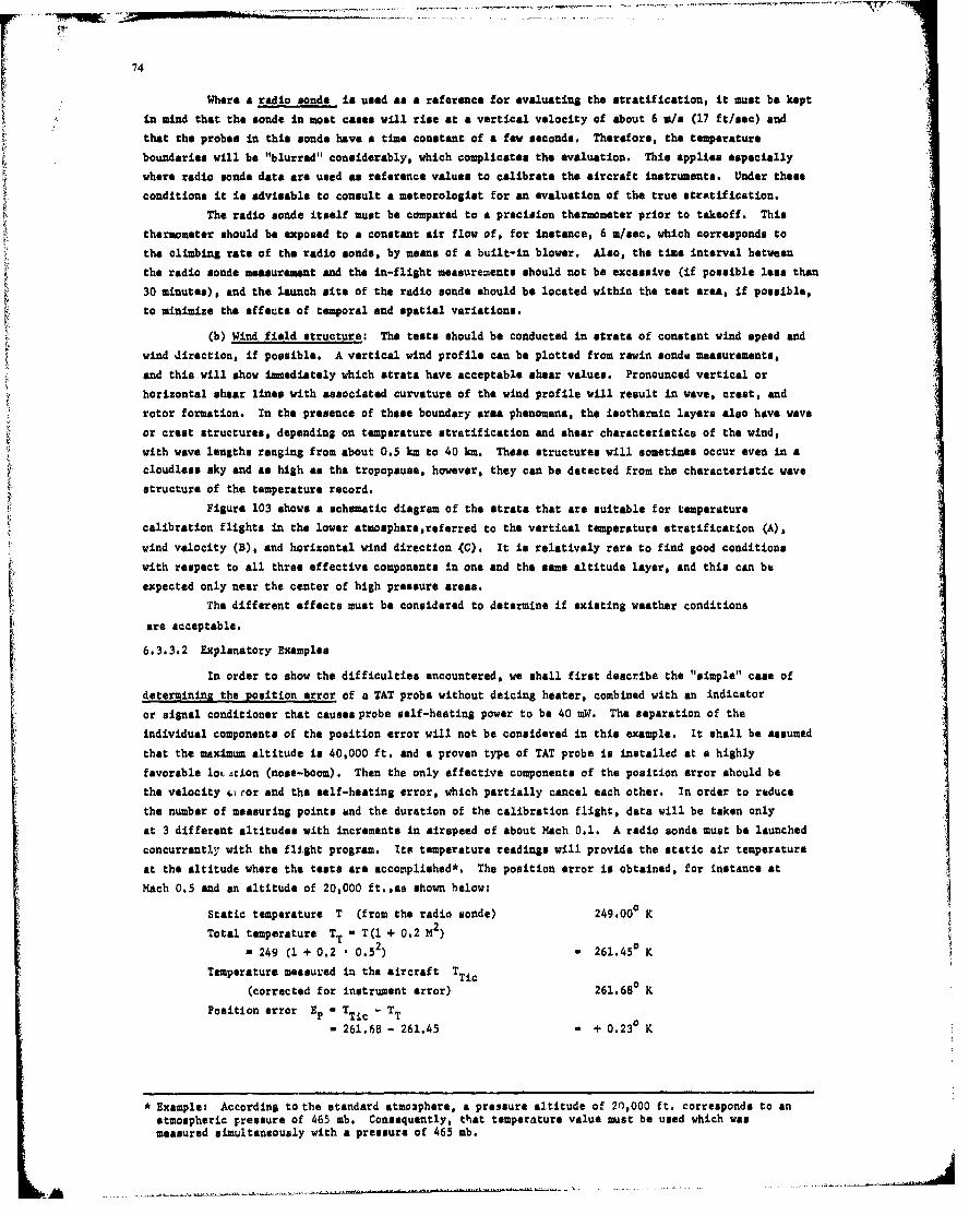
74

Where a radio sonde is used as a reference for evaluating the stratification, it must be kept

in mind that the sonde in most cases will rise at a vertical velocity of about 6 m/s (17 ft/sec) and

that the probes in this sonde have a time constant of a few seconds. Therefore, the temperature

boundaries will be "blurred" considerably, which complicates the evaluation. This applies especially

where radio sonde data are used as reference values to calibrate the aircraft instruments. Under these

conditions it is advisable to consult a meteorologist for an evaluation of the true strAtification.

The radio sonde itself must be compared to a precision thermometer prior to takeoff. This

thermometer should be exposed to a constant air flow of, for instance, 6 m/see, which corresponds to

the climbing rate of the radio sonde, by means of a built-in blower. Also, the time interval between

the radio sonde measurememt and the in-flight measurements should not be excessive (if possible less than

30 minutes), and the launch site of the radio sonde should be located within the test area, if possible$

to minimize the effects of temporal and spatial variations.

(b) Wind field structure: The tests should be conducted in strata of constant wind speed and

wind direction, if possible. A vertical wind profile can be plotted from rawin sonde measurements,

end this will show immediately which strata have acceptable shear values. Pronounced vertical or

horizontal shear lines with associated curvature of the wind profile will result in wave, crest, and

rotor formation. In the presence of these boundary area phenomena, the isothermic layers also have wave

or crest structures, depending on temperature stratification and shear characteristics of the wind,

with wave lengths ranging from about 0.5 km to 40 km. These structures will sometimes occur even in a

cloudless sky and as high as the tropopause, however, they can be detected from the characteristic wave

structure of the temperature record.

Figure 103 shows a schematic diagram of the strata that are suitable for temperature

calibration flights in the lower atmospharereferred to the vertical temperature stratification (A),

wind velocity (B), and horizontal wind direction (C). It is relatively rare to find good conditions

with respect to all three effective components in one and the same altitude layer, and this can be

"expected only near the center of high pressure areas.

The different effects must be considered to determine if existing weather conditions

are acceptable.

6.3.3.2 Explanatory Examples

In order to show the difficulties encountered, we shall first describe the "simple" case of

determinins the position error of a TAT probe without deicing heater, combined with an indicator

or signal conditioner that causes probe self-heating power to be 40 mW. The separation of the

individual components of the position error will not be considered in this example. It shall be assumed

that the maximum altitude is 40,000 ft. and a proven type of TAT probe is installed at a highly

favorable lot -iton (nose-boom). Then the only effective components of the position error should be

the velocity ciror and the self-heating error, which partially cancel each other. In order to reduce

the number of measuring points and the duration of the calibration flight, data will be taken only

at 3 different altitudes with increments in airspeed of about Mach 0.1. A radio sonde must be launched

concurrently with the flight program. Its temperature readings will provide the static air temperature

at the altitude where the tests are accomplished*. The position error is obtained, for instance at

Mach 0.5 and an altitude of 20,000 ft.pas shown below:

Static temperature T (from the radio sonde) 249.000 K

Total temperature TT * T(l + 0.2 M2)0.2

249 (1 + 0.2 . - 261.450 K A

Temperature measured in the aircraft TTic

(corrected for instrument error) 261.680 K

Position error E. - TTic - TT

- 261.68 - 261.45 - + 0.230 K

* Example: According to the standard atmosphere, a pressure altitude of 20,000 ft. corresponds to anatmospheric pressure of 465 mb. Consequently, that temperature value must be used which wasmeasured simultaneously with a pressure of 465 mb.

,-.7- 77777

The theoretically expected result of sucb a series of measurements is plotted in graph form inFigure 100. The practical result of a single series of instrument readings would not, an shown in this

figure, yield the approximately parallel curves but curves that appear to be crossing each other at ran-

dom. There are several reasons for this. Even in the absence of measurement errorq local temporal

variations of static temperature may amount to about +0.50C, especially in the lowest altitude strata

(Reference 104). This means that this effect alone, can be several times greater than the difference

between the measured values at a certain Mach number. Therefore, any attempt to accomplish such

calibration flights under unsuitable meteorological conditions would be meaningless. Although modern

P radio sondes have reliable tolerances as narrov as +0.5 C Co +0.70C, some of them are subject toconsiderable temperature lag errors. If the data from bdveral calibration flights were combined*,

a considerably better picture could be obtained. However, it should be kept in mind that such calibra-

tion flights will take about two hours. Even if the radio sonde were launched in the middle of each

flight, appreciable temperature errors can occur due to changes in the air temperature during the

f light. With a very limited number of measuring points in the area of greatest interest for the

relevant aircraft under normal flight operations (shaded sera. in Figure 100), exact test results are

difficult to obtain, as atmospheric temperature variations exceed the error to be measured.

Figure 101 shows the acquisition of the doicina heat error as an individual component of the

position error through six calibration flights performed at low altitude. These must be repeated at

different altitude levels, of course, because of the altitude dependence of this error. Simply

connecting the measured values obtained in a single flight (corrected for probe calibration error)

would yield a fairly irregular line. The same would still apply for a mean of two flights so that the

practical application of these curves requires considerable smoothing.

This example was selected in order to demonstrate how one individual error can be isolated

from the others. The test can be performed by using two TAT probes (A and B) of the same type and

connecting them alternately via a commutator to the same servoed indicator. Probe A is continuously

operated with probe deicer on during the first half of the flights, while probe B remains unheated.

During the second half of the calibration flights, probe B is continuously heated, while probe A

remains unheated. If both probes are subjected to the smane flow (for instance on the underside of

the nose at a lateral distance of 25 cm from each other), and if the leads between the probes and the

commutator have been adjusted to exactly the same resistance values, all errors will have the same

effect on the measurements taken with probes A and B. These errors then cancel out when the difference

between the measured values of A end B is taken. This difference then is the deicing error. It

should be noted that this does not allow for the indiviudal calibration errors of probes A and B.

These corrections must be applied before plotting the measured data.

If only one probe were available, it would be necessary at each Increment of altitude and

airspeed, after stabilizing the corrected airspeed and altitude indications, to make 60-second measure-

ments with and without the deicer. Sufficient time should be allowed for the probe housing to cool off

completely before attempting rune at the next airspeed. Where this method is used, changes in the airtemperature during the calibration run appear directly in the measured data. These measurements thenbecome meaningless if the atmospheric temperature changes exceed the deicing heat error. In these

cases the use of a radio sonde would not yield any advantages.

The determination of the velocity error shall be discussed as another example. In earlier

times this was done by measuring the recovery factor r and plotting the corrected temperaturesmeasured at different airspeeds as a function of the square of the Hach number (Figure 102a). Since

the recovery factor is a relative value, a single flight at different airspeeds and constant altitude,

where a uniform temperature over the calibration run can be expected, will be sufficient. In many

instances this was accomplished by incrdasing the airspeed at constant acceleration (such as 1 S)

until the aircraft's maximum airspeed was attained, and then decreasing the airspeed at idling engine

CCf. Section 6.4.

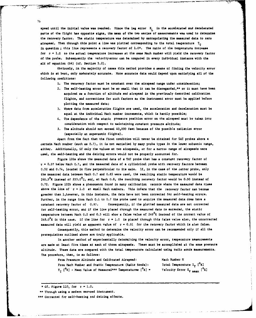
76

speed until the initial value was reached. Since the lag error EL in the accelerated and decelerated

parts of the flight has opposite signa, the mean of the two series of measurements was used to determine

the recovery factor. The static temperature was determined by extrapolating the measured data to zero

airspeed. Then through this point a line was plotted corresponding to the total temperature TT

in question ; this line represents a recovery factor of 1.0*. The ratio of the temperature increase

for r - 1.0 to the actual temperature increases at the same Mach number will yield the recovery factor

of the probe. Subsequently the velocityerror can be computed in every individual instance with the

aid of equation (64) (of. Section 5.2).

Obviously, in the majority of cases this method provides a means of finding the velocity error

which is at bast, only moderately accurate. More accurate data would depend upon satisfying all of the

following conditions:

1. The recovery factor must be constant over the airspeed range under consideration;

2. The self-heating error must be so small that it can be disregarded,** or it must have been

acquired as a function of altitude and airspeed in the previously described calibration

flights, and corrections for such factors as the instrument error must be applied before

plotting the measured data;

3. Where data from acceleration flights are used, the acceleration and deceleration must be

equal at the individual Mach number increments, which is hardly possible;

4. The dependence of the static pressure position error on the airspeed must be taken into

consideration with respect to maintaining constant pressure altitude;

5. The altitude should not exceed 40,000 feet because of the possible radiation error

(especially at supersonic flights).

Apart from the fact that the first condition will never be obtained for TAT probes above a

certain Mach number (such as 0.7), it is not satisfied by many probe types in the lower subsonic range,

either. Additionally, if only the values at two airspeeds, or for a narrow range of airspeeds were

used, the self-heating and the deicing errors would not be properly accounted for.

Figure 102a shows the measured data of a TAT probe that has a constant recovery factor of

r - 0.97 below Mach 0.7, and the measured data of a cylindrical probe with recovery factors between

0.52 and 0.74, located in flow perpendicular to its axis. if, in the case of the latter probe, only

the measured data between Mach 0.7 and 0.85 were used, the resulting static temperature would be

246.5 K instead of 253.0 0 C, and, at Mach 0.8, the resulting recovery factor would be 0.90 instead of

0.72, Figure 102b shows a phenomenon found in many calibration ,records where the measured data rises

above the line of r - 1.0 at small Mach numbers. This infers that the recovery factor can become

greater than l,however, in this instance, the data have not been corrected for self-heating errors.

Further, in the range from Mach 0.1 to 0.7 the probe used to acquire the measured data does have a

constant recovery factor of 0,97. Consequently, if the plotted measured data are not corrected

for self-heating error, and if the line placed through the measured data is extended, the static

temperature between Mach 0.2 and 0,5 will show a false value of 2490K instead of the correct value of

248.0 0 K in this case. If the line for r a 1,0 is placed through this false value also, the uncorrected

measured data will yield an apparent value of r - 0.91 for the recovery factor which is also false.

Consequently, this method to determine the velocity error can be recommended only if all the

prerequisites outlined above are truly applicable.

In another method of experimentally determlaing the velocity error, temperature measurements

are made at least five times at each of three airspeeds. These must be accomplished at the same pressure

altitude. These data are compared with the total temperature calculated using radio sonde measurements.

The procedure, then, is as follows:

From Pressure Altitude and Calibrated Airspeed: Mach Number M

From Mach Number and Static Temperature (Radio Sonde): Total Temperature TT [OKI

TT [OK] - Mean Value of Measured*** Temperatures [oK] - Velocity Error EV mean [OK]

* Cf. Figure 110, for r - 1.0.

** Through using a modern servoed instrument.

*** Corrected for self-heating tnd deicing effects.

L A.

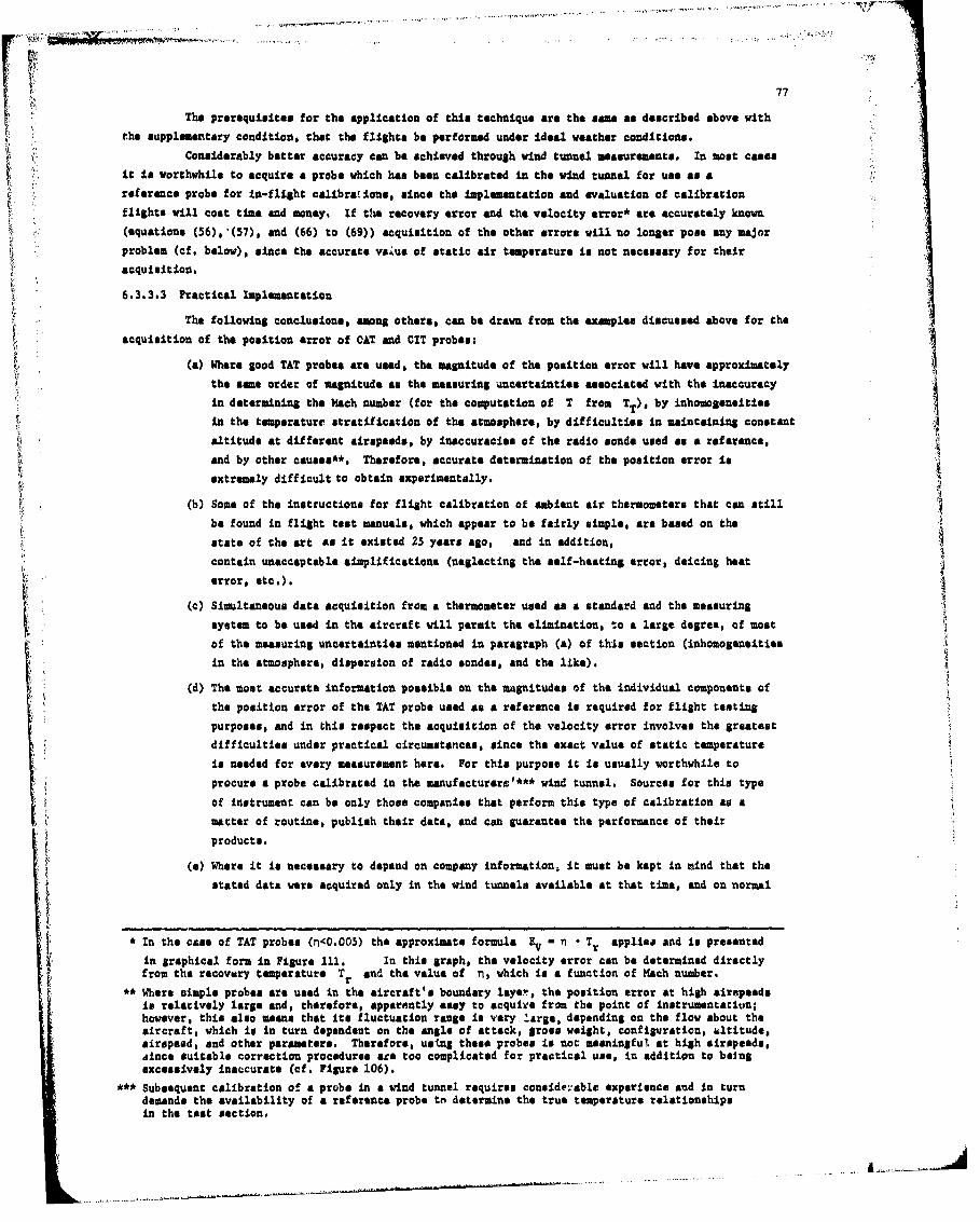
77

The prerequisites for the application of this technique are the same as described above vith

the supplementary condition, chat the flights be performed under ideal weather conditions.

Considerably better accuracy can be achieved through wind tunnel measurements. In most cases

it Is worthwhile to acquire a probe which has been calibrated in the vind tunnel for use as a

reference probe for in-flight calibrations, since the implementation and evaluation of calibration

flights will cost time and money. If the recovery error and the velocity error* are accurately known

(equations (56), (57), and (66) to (69)) acquisition of the other errors will no longer pose any major

problem (cf. below), since the accurate vaiua of static air temperature is not necessary for their

acquisition.

6.3.3.3 Practical Implementation

The following conclusione, among others, can be drawn from the examples discussed above for the

acquisition of the position error of CAT and CIT probes:

(a) Where good TAT probes are used, the magnitude of the position error will have approximately

the same order of magnitude as the measurina uncertainties associated with the inaccuracy

in determining the Mach number (for the computation of T from TT), by inhomogeneities

in the temperature stratification of the atmosphere, by difficulties in maintaining constant

altitude at different airspeeds, by inaccuracies of the radio sonde used as a reference,

and by other causes**. Therefore, accurate determination of the position error is

extremely difficult to obtain experimentally.

(b) Some of the instructions for flight calibration of ambient air thermometers that can still

be found in flight test manuals, which appear to be fairly simple, are based on the

state of the art as it existed 25 years ago, and in addition,

contain unacceptable simplifications (neglecting the self-heating error, deicing heat

error, etc.).

(c) Simultaneous data acquisition from a thermometer used as a standard and the measuring

system to be used in the aircraft will permit the elimination, to a large degree, of most

of the measuring uncertainties mentioned in paragraph (a) of this section (inhomogansities

in the atmosphere, dispersion of radio sondes, and the like).

"(d) The moat accurate information possible on the magnitudes of the individual components of

the position error of the TAT probe used as a reference is required for flight testing

purposes, and in this respect the acquisition of the velocity error involves the greatest

difficulties under practical circumstances, since the exact value of static temperature

is needed for every measurement here. For this purpose it is usually worthwhile to

procure a probe calibrated in the manufacturers'*** wind tunnel. Sources for this type

of instrument can be only those companies that perform this type of calibration as omatter of routine, publish their data, and can gularatee the performance of their

products.

(a) Where it is necessary to depend on company information, it must be kept in mind that the

stated data were acquired only in the wind tunnels available at that tine, and on normal

* In the case of TAT probes (n<0.005) the approximate formula E " n , T. applies and is presented

in graphical form in Figure 111. In this graph, the velocity error can be determined directlyfrom the recovery temperature Tr and the value of n, which is a function of Mach number.

** Where aimple probes are used in the aircraft's boundary layer, the position error at high airspeedsis relatively large and, therefore, apparnntly easy to acquire from the point of instrumentation;however, this also means that its fluctuation range is very large, depending on the flow about theaircraft, which is in turn dependent on the angle of attack, pross weight, configuration, ultitude,airspeed, and other parameters. Therefore, using these probes is not meaningful at high airspeeds,dince suitable correction procedures &te too complicated for practical use, in addition to beingexcessively inaccurate (cf. Figure 106).

*** Subsequent calibration of a probe in a wind tunnel requires consides.able experience and in turndemands the availability of a reference probe to determine the true temperature relationshipsin the test section.

78

aircraft. Information on in-flight data outside the normal flight corridor, for instance

at Mach 0.1 and 80,000 ft., could at best be acquired through computation and must,

therefore,be considered with great caution. On the other hand, information for the

normal flight corridor is usually conservative, since compliance with these data must be

proved to certain consumers in very stringent test procedures.

(f) For flight testing purposes the position error of the temperature probe is of interest with

respect to all those combinations of altitude and airspeed within the capability of

the test aircraft. However, in practical flight operations many aircraft in most cases

remain within a narrow range about a nominal flight profile (cf. the shaded area in

Figure 100) which makes it possible to use greatly simplified corrections for the

indicated data.

A suitable reference thermometer, which has been mentioned several tines is a TAT probe,

Type MS 27 188 - 1 (Model 102 CD 2U), calibrated for the recovery error*, with a hermetically sealed

Pt element of 500 ohms having close tolerances, and a servo instrument with recording outputs (such as

BH 180 or BH 187 "Auto-Tamp" by Howell Instr. Co., or the Temperature Servo Indicator 25001 by Betzelt

GmbH Muenchen,Germany). They have an indicator accuracy of +O.2 0 C and a self-heating effect so small

(less than 0.04 mW) that it can be disregarded**. Consequently, the instrument error (including probe

calibration error) is about +0.23eC, provided that the system was carefully corrected for lead

resistances after installation into the aircraft (cf. Section 6.3.2). When this type of probe can be

installed at a favorable location (such as a nose boom), and when the probe deicer is turned off,

only the velocity error is significant so that the indication cor.iesponds directly to the recovery

temperature, T The associated absolute value of the velocity error E is easily determined fromr

the values of the recovery error, and the recovery temperature, which are dependent on the Mach number

(EV z T Tr[K], cf. Figure 111). Consequently, the temperature values read, or recorded, using this

thermometer, require only a correction for the velocity error in order to acquire the associated total

temperature as a reference value for other thermometers that must be calibrated.

Subsequently, during calibration flights, direct comparison of the reference thermometer with

the thermometer to be calibrated will yield the overall position error of the latter as well as its

individual components. The tabulation below illustrates a distinction between two cases of Interest.

In case (a) the stipulation is that the probe to be calibrated has the same nominal resistance (for

instance, 500 ohms) and the same characteristic*** as the reference probe. In that L.... os $1cwn in

Figure 104a, a commutator should be used. In case (b) it is assumed that different probe resistances

or characteristics exist so that it is not possible to commutate. In both cases, it is stipulated that

the measurements are performed at constant airspeed and altitude**** so that the lag error can be

neglected. Practically, its magnitude could be determined with adequate accuracy only in an

appropriately equipped wind tunnel.

Overall position error***** (la) as in (lb), no commutation.

(lb) Comparison of the indication of the reference

thermometer, corrected for the velocity irror

(- total temperature), with the indicnation oL

the thermometer to be calibrated, corrected

for instrument error.

• Less favorable than wind tunnel calib7:atlon is in-flight calibrarion performed with the aid

of a radio sonde, as described above.** The Betzelt indicator also has provisions for switching to a Mach-fuuction potantiometer for

direct indication of Static Air Temperature (SAT) (cf. figure 33).

•** Caution: Normal platinum probes and platinum probes with narrowed tolerances (PCI elements)have different characteristics; tha same &ppltes, for instance, to 100 ohm Pt probes and100 ohm Ni probes.

•*** These altitudes are selected after evaluation of the radio sondt mission that is nearest withrespect to time and location.

•**** Deicer turned off on both probes.

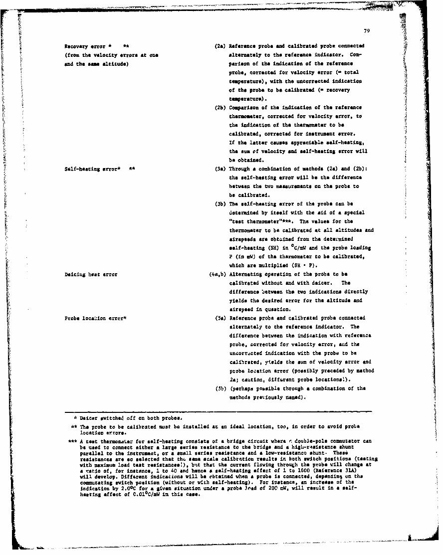
79

Recovery error * ** (2a) Reference probe and calibrated probe connected

(from the velocity errors at one alternately to the reference indicator. Con-

and the some altitude) perison of the indication of the reference

probe, corrected for velocity error (- total

temperature), with the uncorrected indication

of the probe to be calibrated (- recovery

temperature).

(2b) Comparison of the indication of the reference

thermometer, corrected for velocity error, to A

the indication of the thermometer to be

calibrated, corrected for instrument error.

If the letter causes appreciable self-heating,

the sum of velocity and eelf-heating error will

be obtained.

Self-heating error* ** (3a) Through a combination of methods (2a) and (2b):

"the self-heating error will be the difference

between the two measurements on the probe to

be calibrated.

(3b) The self-heating error of the probe can be

determined by itself with the aid of a special

"test thermometer"***. The values for the

thermometer to be calibrated at all altitudes and

airspeeds are obtained from the deteoimned

self-heating (SH) in 0 C/mW and the probe loading

P (in mW) of the thermometer to be calibrated,

which are multiplied (SH• P).

Deiciao heat error (4a,b) Alternating operation of the probe to be

calibrated without and with deicer. The

difference between the two indications directly

yields the desired error for the altitude and

airspeed in question.

Probe loc1aion error* (Sa) Reference probe and calibrated probe connected

alternately to the reference indicator. The

difference between the indication with reference

probe, corrected for velocity error, and the

uncorrected indication with the probe to be

calibrated, yields the sum of velocity error and

probe location error (possibly preceded by method

2a; caution, diffirent probe locations!).

(Sb) (perhaps possible through a combination of the

methods previously named).

SDeicer switched off on both probes.

** The probe to be calibrated must be installed at an ideal location, too, in order to avoid probelocation errors.

•** A test thermometer for self-heating consists of a bridge circuit where , double-pole commutator canbe used to connect either a large series resistance to the bridge and a high-r4sistance shuntparallel to the inctrumaat, or a small series resistance and a low-resistanco shunt. Theseresistances are so selected that th. mane scale calibrntion results in both switch positions (testingwith maximum load test resistances:), but that the current flowing through the probe will change ata tatio of, for instance, 1 to 40 and hence a self-heating effect of 1 to 1600 (Reference 31A)will develop. Different indications will be obtained when a probe is connected, depandinS un thacommutating switch position (without or with self-heating). For instance, an increase of theindication by 2.OOC for a given situation under a probe load of 20C mW, will result in a self-heating effect of C.Ol°C/mW in this case.

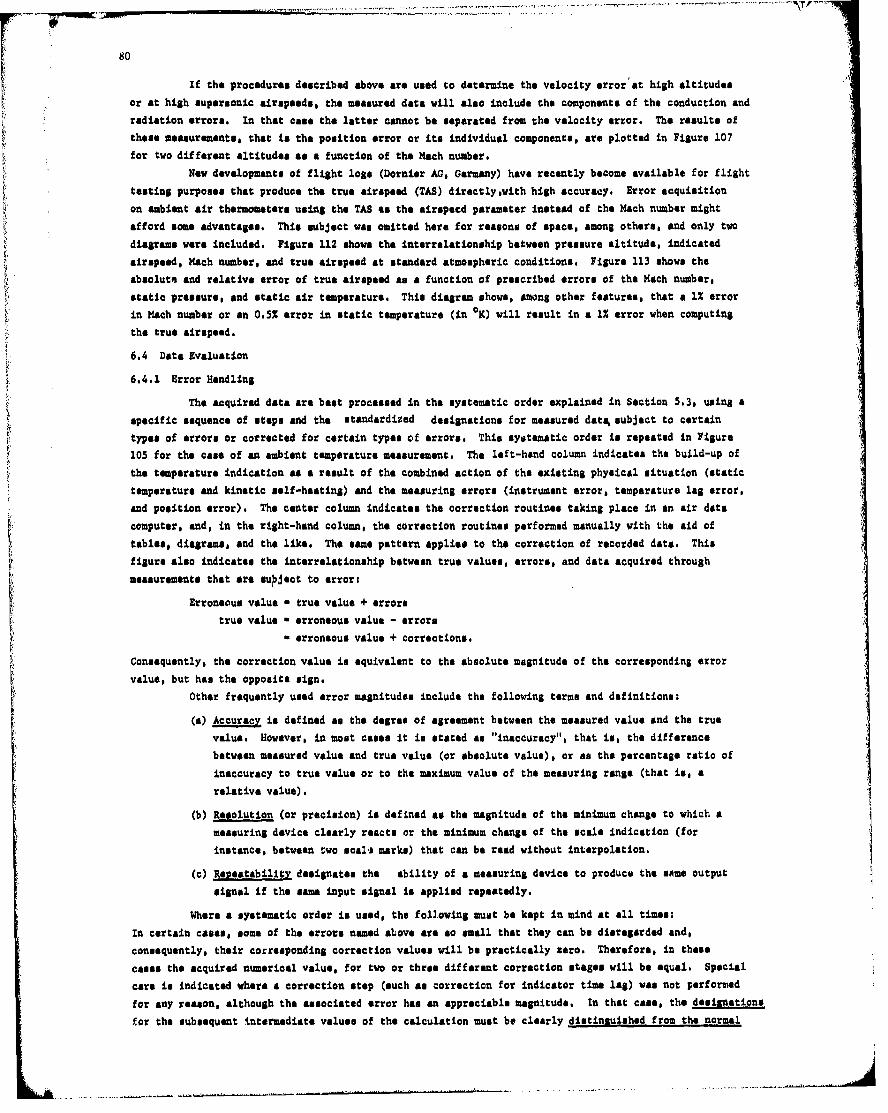
80

If the procedures described above are used to determine the velocity error at high altitudesor at high supersonic airspeeds, the measured data will also include the components of the conduction andradiation errors. In that case the latter cannot be separated from the velocity error. The results of

these measurements, that is the position error or its individual components, are plotted in Figure 107

for two different altitudes as a function of the Mach number.

New developments of flight logs (Dornier AG, Germany) have recently become available for flighttesting purposes that produce the true airspeed (TAS) directly,with high accuracy. Error acquisitionon ambient air thermometers using the TAS an the airspeed parameter instead of the Mach number mightafford some advantages. This subject was omitted here for reasons of space, among others, and only two

diagrams were included. Figure 112 shows the interrelationship between pressure altitude, Indicated

airspeed, Koch number, and true airspeed at standard atmospheric conditions, Figure 113 shows theabsolute, and relative error of true airspeed as a function of prescribed error. of the Mach number,

static pressure, and static air temperature. This diagram shows, among other features, that a 1% errorin Mach number or an 0.52 error in static temperature (in 0K) will result in a 1% error when computing

the true airspeed.

6.4 Data Evaluation

6,4.1 Error Handling

The acquired data are best processed in the systematic order explained in Section 5.3, using a

specific sequence of steps and the standardized designations for measured datsý subject to certaintypes of errors or corrected for certain types of error.. This systematic order is repeated in Figure

105 for the case of an ambient temperature measurement. The left-hand column indicates the build-up ofthe temperature indication as a result of the combined action of the existing physical situation (statictemperature and kinetic self-heating) and the measuring error. (instrument error, temperature lag error.

and position error). The center column indicates the correction routines taking place in an air datacomputer, and, in the right-hand column, the correction routines performed manually with the aid of

tables, diagrams, and the like. The same pattern applies to the correction of recorded data. This

figure also indicates the interrelationship between true values, errors, and data acquired throughmeasurements that are supject to error-

Erroneous value n true value + errorstrue value a erroneous value - errors

- erroneous value + corrections.

Consequently, the correction value is equivalent to the absolute magnitude of the corresponding error

value, but ha. the opposite sign.

Other frequently used error magnitudes include the following terms and definitions:

(a) Accuracy is defined as the degree of agreement between the measured value and the truevalue. However, in most cases it is stated as "inaccuracy", that is, the differencebetween measured value and true value (or absolute value), or as the percentage ratio ofinaccuracy to true value or to the maximum value of the measuring rsnge (that is, arelative value).

(b) Resiolution (or precision) is defined as the magnitude of the minimum change to which a

measuring device clearly reacts or the minimum change of the scale indication (for

instance, between two scal-i marks) that can be read without interpolation.

(c) Repeatability designates the ability of a measuring device to produce the some output

signal If the same input signal is applied repeatedly.

Where a systematic order is used, the following must be kept in mind at all times:

In certain cases, some of the errors named above are so small that they can be disregarded and,

consequently, their corresponding correction values will be practically zero. Therefore, in thesecases the acquired numerical value, for two or three different correction stages will be equal. Special

care is indicated where a correction step (such as correction for indicator time lag) was not performed

for any reason, although the associated error has an appreciable magnitude. In that case, the designations

for the subsequent intermediate values of the calculation must be clearly distinguished from the normal

__ 81case (for instance, stating "total temperature, not corrected for indicator time la$ error"). Only themost important error categories (pnsition error, temperature lU& error, and instrument error) are named

in the systematic order shown in this paper. In certain boundary cases, the group of meteorological

errors can be added, which is bc..: processed in conjunction with the position errors. Since each error

group consists of individual errors, their overall value must be determined from the individual error

values in a secondary calculation not included here, before these are entered into the systen (cf. below),

This is the reason why the term "recovery temperature" does not appear in Figure 103, since it is merely

an intermediate value for the calculation of the position error.

Since any computation routine is a time-consuming nuisance during the measurement period, in

addition to introducing new sources of error, attempts must be made beforehand to reduce the number of

error types and their magnitudes as much as possible. All avoidable err&or, such as read-out errors,

errors due to recording paper shrinkage, errors duc to using instruments with excessive self-heatinl

characteristics, probe location errors, and the like*, must be avoided using appropriate instrumentation

techniques. Also, every care must be taken to ensure that the absolute magnitudes of the remaining

unavoidable errors are kept as small as possible. The reader is referred to the appropriate discussion

in the preneding chapters and to Table 8 in Section 6.1.1.

The errors encountered in accomplishing the different calibrations (according to Section 6.3)

can be generally subdivided as follows:

Random errors. These are errors with a statistical distribution of values and indefinite

sign (positive or negative).

Example: E =_+ 0.23°C.

Systematicaerrors have a certain magnitude and definite sign for a given nst of circumstances,

Example: E I + 0.46°C (at scale point + 25.0°C).

However, because of the limited measuring accuracy, they are frequently encountered as systematic errors

with uncertainty, that have a definite sign but a magnitude which is variable within certain limits,

Example: Z a + 0.52°-C + 0.260 C.

Systematic errors can be corrected, since they are determined with respect to sign and magnitude.

Several individual systematic errors can be combined through addition into a single magnitude for an

error group. Random errors, like the uncertainties of systemartic errors, have Alternating signs

and therefore partially cancel each other, so that they must be combined on a statistical basis, A good

approximation for this purpose is provided by the square root of the squared absolute magnitudes of

random errors (RS sumamtion):

+ _+ E +E +E2+ . (89)

where E., Eb, etc are random errors, generally expressed in standard deviattions (of. page 82).Systematic errors with uncertainty can develop, for instance, as follows: The error,.. E is

normally defined as the deviation of the measured value X from the true value XC. Even with carefulexecution of a series of measurements specifically designed to dstermine, for instance, the scale

error ESC, the readings taken at a certain point on the scale (such as +250C) during twenty repetitions

of the measurement will yield 20 different measured values (X, X26 . . . X20), which will show a certain

amount of dispersion in their values**.

COnsequently, we obtain for n measurements of a point n measured values: X1 , X , . . . Xn,

The true value is XC.

The measured error values are:

v e.8. temperature-sensitive DC-amplifiers or oscillators in telemetry equipment.

**This is due, among other causes, to the fact that both the instrument and the test equipment connectedto it have a finite accuracy. In addition, there are environmental effects, read-out errors, etc.

• * This i8........................................................................................cte

•' 82

Bl X -,,/: I , I - c

. E2 -X 2 -C

Y En -Xn -Xc,

The arithmetic mean value of the error is:

- (E1 + E2 - . . .÷ En)/n (90)

The mean arrox spread a ist

u-[(El &E) + (E2 - E) + + (En -) Jb In (91)

Thus we can obtain a systematic error with uncertainty in the following form:

E - a (for example, ESC - + 1.97°C + 0.045°C).

Where it is intended to add this error to another systematic error with uncertainty (for instance,

EW - 0.470C + 0.050°C), the following procedure is followed:

Evral "+ 1.970C - 0,470C + ±0,0452 + 0,0502

- + 1.50°C + 0.067oC

Mostly, the standard deviation a is used instead of the mean error spread a, in which case:

E -E lo[for example, E. + 0.900C O.0l70 C (l)j.

The standard deviation o is defined as follows:

•/ E - Eh2 + (E '- B)2 . . . .+ (; - E)2

n

Generally, measurement errors can be represented by a gaussian distribution. In this case

the probability that an error of a particular measurement falls in the interval E ± 1 0 , E + 2 ,

or Ei .3a is 69.3%, 95.4%, or 99.7%, respectively.

For a gsaussian distribution the value of the standard deviation a can be expressed in termsof the mean error spread ot by:

o~cf T12 25 (92)o .a • 1.25 01•2

Now we can transform the form of the error ESC mentioned above through multiplication

(±0.0450 C . 1.25) into*:

ESC a + 1.97 C + 0.0560C; (la).

* If needed we can also obtain the form for 3a by multiplication (. 0.056 3): ESC + 1.970 C +0.168°C; (30)

.........

83

The comoination of several individual errors into one overall errot is achieved, in the examples used

here, through direct addition of the systematic components and forming the square root of the sum of

the squared statistical error components (RSS summation of the uncertainties), as follows:

Eoverall C +Ew

1.97 C + 0.90°C + 0562 + 04017•°C

o o+ 2.87 C + 0.0575 C; (10)

It is seen that, in the combination of uncertainties or standard deviations, as well as

statistically distributed errors (random errors), it is always the maximum value that governs the

overall value. In most instances, all values can be disregarded if they are smaller than one fifth of

the maximum value. Moreover, it is impractical to calculate with a greatly different number of

integers behind the decimal point, since this will not increase the accuracy but merely the computation

effort. Therefore, numerical values with too many decimals should be rounded off.

In the calculation routine described above, the overall error for a certain point of the

instrument scale (indication + 250 C) was determined. If this routine is repeated for a number N of

additional scale points, a different mean for the overall error will be obtained for every poinc on

the scale, where the standard deviation can assume different values. If, as in the example of

Figure lOlb, the variation of the means is small, an overall error with uncertainty can be derived

from the number N of the overall errors that are each valid only for one single point. Here, the

sum of the means and the separate standard deviations uan be combined as follows:

Eoverall" E(B + . + E j)/N4 /(Gl +01 +0 (93)

Thus we obtain a single value that is valid for the entire range with sufficient accuracy.

The same procedure would be possible for an error profile of the type shown in Figure lOla, for low

Mach numbers, but it would yield a false statement on the characteristic error profile over a large

part of the range.

Practical examples for the acquisition of the overall error as a function of different

parameters are provided below. However, it should be noted here that, in addition to the linear error

distribution discussed above, where the uncertainty boundaries are located symmetrically to the mean

value, there are also nonlinear error distributions where the uncertainty boundaries are located

asymmetrically to the mean value. One typical example of this situation is the velocity error. For

instance, if the recovery factor fluctuates by + 0.1 in the subsonic range, the velocity error will

have an asymmetrical error distribution, Figure 106* shows a velocity error of EV U -Z.3OC + 1.45/

-1.05 C for Mach 0.5. Conversion into a symmetrical form (by forming a simple mean of uncertainty),

Ev - -2.3 0 C + 1.25°C, is not correct, but in this case, is acceptable in place of cumbersome computationroutines, because the error value so obtained is located "on the safe side" (conservative), meaning that

it is more likely too high than too low. This form of a systematic error with symmetrical uncertainty

can be combined subsequently with other errors of any type, by the procedure described above.

in our discussion of the individual components of the position error in Section 5.2, we

mentioned only a few systematic errors that always have a positive sign (such as the self-heating error

ESH and the deicing heat error EDH), or always a negative sign (such as the velocily error EV and

the attitude error Ea). Other systematic errors :an have different signs, depending on prevailing

* These figures will be discussed at greater length in the section which follows.

84

conditions (heat addition greater than heat subtraction, and vice versa), for instance, the heat

conduction error Ec and the radiation error ER. When all of these components are combined into the

position error, a systematic overall error will arise that has a positive sip below a certain Mach

number, passes through zero at this Mach number, and then has a negative sign (cf. Figures 108 and 109)*.

The uncer iinty or standard deviation of the position error will be very great in the presence of a self-

heating error and/or a deicing heat error at extremely low airspeeds, but will decrease very rapidly

with increasing airspeed, and rise again gradually above about Mach 0.2. Where these two errors are

absent, the uncertainty of standard deviation will be almost equal to zero at very slow airspeeds, and

will rise slowly with increasing airspeed, as a function of the velocity error (cf. Figures 106 and 107)*.

In most instances, the temperature lag error can be -disregarded, since the measurements arc

normally performed in a steady-state flight (that is, at constant altitude and airspeed). Where the

probe has a simple time constant, and in the event that temperature jumps or temperature changes at

constant temperature gradient occur during the measurement, these could be corrected as described in

Section 5.2.3. Since it is very difficult, in most cases, to determine whether temperatures belong to

one of these two types, or whether they have a sinusoidal pattern, rather elaborate mathematical treatment

will usually become necessary (cf. Reference 3). These are subject to great uncertainty, especially

in those cases where measurements acquired in accelerated flights are to be evaluated**. Measurements

using probes that have several time constants are normally even more difficult to correct. However,

in the case of the probe shown in Figure 83, it can be expected that, at airspeeds above Mach 0.2

(that Is, where the tine constant has values of T2 < 0.4 see), the error will be less than 1% of the

temperature change within one second after its occurrence, so that it can be disregarded for practical

purposes.

The components of the instrument error E1 (probe calibration error 2CAL and scale error

Esc) are dependent on the temperature measured in every instance, and no regular interrelationship

exists between error magnitude and temperature. These errors are due to random variations in the

production process. These must be measured individually for every probe and instrument (cf. Figures

106 and 108)* , unless units with close tolerances and servoed indicators, or signal conditioners with

extremely small errors, are used (cf. Figure 107)* . The electric lead error EW is dependent on the

indicated temperature also, but it can be made so small, through use of three-wire or four-wire leads

if low-resistance elements are used, that it can be disregarded,

6.4.2 Data Evaluation and Error Correction

Here, data evaluation and error correction are discussed using the example of ambient

fIemperature measurement, and the values illustrated in the form of tables and diagrams.

As a rule we must distinguish between two cases:

(a) if the data are needed over the entire flight envelope of the aircraft, the dependence of

all errors on Mach number must be plotted for the different altitudes at increments of

typically 10,000 ft. This rather voluminous effort will be required in most instances for

flight tests of civil as well as military aircraft.

(b) In the case of aircraft used for ci,.-il transportation or -imilar use, a

certain range about a standard flight profile will be exceeded only under exceptional

circumstances, Possibly, two such flight profiles can suffice, where an aircraft is

employed in both short-range and long-range flights.

In the first case, five diagrams may be required. This could even double in number where both

operations with and without probe deicer are to be covered. However, in the second case, tha probe de-

icer system will always be turned on at take-off, so that one or two diagrams will suffice. In the

case of VTOL aircraft or helicopters, relationships will possibly range between these two boundary cases.

* These figures are discussed in-more detail in the section which follows.

** The time lag e-ror of the recorded pressure values must first be corrected also.

85

As a rule, it will be sufficient to plot the appropriate values of the standard atsphere asstatic temperatures for the different altitudes. However, it should be pointed out that, near the

ground, the static temperature can deviate considerably from the standard value. In those cases where

the Instrument errors that sae dependent on the Indicated temperature reach large values, it may prove

necessary to prepare two or three diagrams for the lowest altitude level (for instance, 1000 ft)*,

since the indicated temperature is a function of at least static tmperature and Mach number. For

practical purposes (meaning the correction of the indicated values in the aircraft), the usual procedure

is to establish a small correction table from the graph presentations, possibly stating the applicable

range of the table.

The first type of data evaluation is shown In Figure 106 fov a 1200 ohm flush-bulb probe

with ratio meter at an altitude of 100 ft and a static temperature of + 16°C. The same presentations

would have to be prepared for the altitudes of 10,000 ft, 20,000 ft, and 30,000 ft (depending on theceiling of the aircraft). In the upper part of Figure 106, the self-heating error S and the airspeed

error 1. with its dispersion range, are plotted versus the Mach number. Sinc the components of the

Instrument error depend on the temperature of the probe or on the prevailing Indication of the

instrument, the probe calibration error , the scale error ESC and their sm, the Instrument

error 2 (each measured individually in the laboratory) are plotted in the lower part of this figure as

a function of temperature. The electric lead error was considered negligible, since the probe

has very high resistance and is operated in a three-wire configuration. In order to be able to transfer

the Instrument error to the upper part of the figure as a function of Mach number, we must firstdetermine the recovery temperatures Tr associated with the Individual Mach numbers, assuming a m--a

recovery factor of r - 0.85** for the altitude in question and for the static temperature prevailing

there, using Figure 110. The values of the Instrument error that are associated with the recovery

temperature values found by this procedure can be plotted subsequently in the upper diagram versus the

corresponding Mach numbers. Addition of self-heating error, Instrument error, and velocity error (man)

will yield the solid line of the overall error, by which the mean of the indication deviates from thetotal temperature. The uncertainty of the velocity error would have to be displaced in accordance with

the overall error of -2.8°C with an uncertainty of about + 0.8 0 C*** at Mach 0.4. To be quite precise,

specific uncertainties would have to be taken Into consideration for the other error values as well,

but in the case shown here these are very small and can therefore be disregarded. The uncertainty would

Increase rapidly with increasing airspeed and would reach a value of about + 40C at Mach 0.85, for

instance, making the measurement useless.

It is seen from this example that, in the case of simple temperature probes located in the

aircraft's boundary layer, the airspeed error, and dispersion, is so large at intermediate Mach numbers

that it overshadovs all other errors. Further, it is seen that the effort Involved in the calibration

and in the summation of the instrument errors that are dependent on the indicated temperature, and the

position errors that are dependent on the Mach number are extremely laborious and time-consuming If

an acceptable accuracy is to be obtained.

The opposite ezample is illustrated in Figure 107, where the error components for a total

temperature probe of 500 ohms and a servoed indicator are shown. In this system, the rsplacement of theprobe or the instrument requires only the adjustment of the line compensation for the Instrument at two

measuring points. In that case, the instrument error, like its individual errors, is defined by

its tolerance limits:

+A_ - +_. + - . + 0.2 - + 0.2?c (94)

(cf. the upper part of the figure). This value is not dependent on the indicated temperature, since the

• This corresponds approximately to minimum altitude, except for take-off end landing.

** To simplify the presentativc., a very favorable probe location was assumed; this may result in analmost constant recovery factor.

e** In this case, dispersion range should be esymmetrical: +0.90C, -0.70C; it can be rounded off withlittle error to + 0.8°C, cf. above.

86

limits fo0r Es and E apply for the enir temperature range. Where probes with normal tolerancesare used (cf.* the dotted curves), thia would not be the case.* However,* during normal climbing and let-

down flights the temperature in the subsonic airspeed range would be displaced to such a degree that the

probe calibration error should not exceed the limits of +0. 30 C. The result would be an instrument error

V ~of +0.36 C over the entire subsonic range, that would include the scale error limits. The canter diagram

shove the deicing heat error ZHof a probe housing with one element*, and the velocity error Ewith uncertainties up to an altitude of about 1000 ft. The lower diagram shows the corresponding values

for the stratosphere. Thia type of a T&T probe will also yield an asymmetrical measured value

distribution, where the mean will be located nearer to the smaller values. Consequently, if the

probe deicer were, turned off, only thq velocity error Eýwould have an effect, and its uncertainty

would have to be summd (after conversion to symmetrical values) with the uncertainty of the instrument

error (Rss sumation).* If the probe deicer were turned on, the velocity error Evwould be compensated

by the deicing haat error %Hat about Mach 0.35 in sea level flight, and Mach 0.55 at am altitude of

40,000 ft. At greater airspeecs, the velocity error would be predominant, and at slower airspeeds

the deicing heat error predominates. The resulting overall error** was not plotted in this figure, but

the self-heating; error E Hwhen using galvanometers and ratio meters is shown for comparison purposes.

This error is hardly noticeable in the case of good servoed instruments.

Figure 108 shows an ea-, le for case (b) identified above, where the resulting overall error

is shown for a flight profile with Mach 0.2 at sea level, Mach 0.85 at 40,000 ft, and Mach 2.0 at

50,000 ft, using servoed instruments with enclosed and exposed elements, each set with and without

probe deicer system.,

Figure 109 shows a combination of a probe having an enclosed 500 ohm platinum element with a

galvanometer and with a ratio meter, for the same flight profile. The means and the associated

uncertainties are represented for the conditions with and without probe deicer.* In this Caae the

tolerance limits of the instrument error and probe calibration error were entered into the calculation of

f the uncertainty, since the stipulation bad been made that the probes and the indicators should be

interchangeable without individual recalibration. It is Rsee from this figure that this requirement,

which is made by some aircraft operators, results in uncertainties or tolerance limits ranging from0 0

+ 1.5 C to 2.5 C, in spite oZ7 using TAT probes. Under these conditions the employment of probes havingclose tolerances would hardly yield en advantage, since the instrument tolerances are the governing

factor. However, where simple probes are used in the aircraft's boundary layer ***, the uncertainties

would incresas very rapidly at airspeed. in excess of about Mach 0.4. The case of a combination of a

TAT probes (with normal calibration tolerances) with a galvanometer is shown for comparison purposes,

both elements being calibrated in the laboratory. This results in a considerably narrowed uncertainty.

cf. the shaded zone, of about +0.5 0C. However, the mean can have such en unfavorable profile versus.

the Mach number that a strange correction table would result.

The following conclusions can be drawn from these figures:

(a) The customary combination of TAT probe with enclosed element (normal tolerances) and

galvanometer or ratio meter will permit only moderate accuracy with a dispersion of + 2.5 0

in the case of the galvanometer or + 1.5 0C for the ratio meter (applicable for measuring

ranges from -50 0 C to +70%). unless correction tables are used.

(b) If an instrument error correction (composed from individual calibrations of instrument

and probe), which is dependent on the indicated temperature, is allowed for the

equipment array named above, supplemented by ar, additional correction for the position

error (velocity error + deicing heat error), which is dependent on the Mach number,

cuite reasonable accuracy will be achieved with en uncertainty of about + 0.5 a .

However, the correction tables must list a large number of values and become too

cumbersome to handle in practical application.

*Deicing heat error is considerably greater in housings with two elements (by sore than 10C at slowairspeeds).

**Cf. Figure 108.seAs is the case in Figure 106.

(c) The beat accuracy (0 to + 0.250C with an uncertainty of + 0.25 C) is provided by a probe

with an open-wire element and close tolerances, combined with a servoed indicator. In

that case the correction tables may become entirely superfluous. However, because of

their fragile nature, these open-wire elements are hardly feasible for sustained use In

supersonic aircraft.

(d) Vary good results (0 to -0.6 0 C + 0.32°C) are achieved with probes having sealed elenents

and close tolerances, combined with a servoed indicator. In this case, the correction

tables could be eliminated for many types of applications, and where it is needed, the

table will be much simpler than it is in the case of itam (b) above.

An additional inaccuracy of + 0.5°C will develop during the conversion of total temperature

to static temperature (using tables or Figure 110, line r - 1.00), increasing the uncertainty to a

maxium of +2.6°C or + 1.6°C, respectively, in case (a), and to about + 0.6 0 C in case (d).

In an air data computer, the corrections for the systematic error component of the output

signal (that is fed to other systems and indicators) should be done automatically. In that case, the

theoretical uncertainty for the static temperature in a computer for the subsonic airspeed range

(at a mean error of + 0.01 Mach in the acquisition of the Mach number) would have a maxinim of + 0.8°C*.

However, the "guarantaed" values are + 3.0°C from Mach 0.3 upward for the older systems (referred to the

* indication on the instrument), because of the difficulties involved in acquiring the Mach number at the

*- low airspeeds. However, in this respect, the following should be noted:

The "guaranteed" values of air data computers apply almost always with the stipulation that

the position error at the inputs for static and total pressure are present only above Mach 0.4, end

that the position error table acquired during the flight test program is valid for all aircraft of the

sane type and permits 1002 correction. Also, it is usually stipulated that the velocity error be the

only appreciable error of the temperature probe (which in the case of TAT probes has been reduced to the

magnitude of the other errors). Moreover, in the majority of cases the computer manufacturers prescribe

neither the selection of the TAT probe (for instance, types with close tolerances and two elements),

nor that the deicer be turned on (while taxiing and in flight). And in any event, the temperature

probes are in most cases operated at greatly excessive voltages, so that self-heating will assuma

considerable values. Consequently, it is worthy of examination whether the "guaranteed temperature

values" are maintained only with a substitute resistance (that can be loaded as desired) or whether

they can be maintained with a probe exposed to an air flow, taking into consideration whether the

probe deicer is turned on or off.

Consequently, there are the following uncertainties as absolute and relative values for the

determination of the static air temperature, the relative values referred to a static air temperature

"of 216.70K - - 56.50C in the stratosphere* (for airspeeds up to about Mach 2.3 and altitudes below about

60,000 ft):

Conversion Galvanometer +2.6 0 C - +1.2%from the TAT Ratio-meter T1.60C - +0.774indication Sarvoed instrument .0.60C - +0.28%

(With PCI)

Air data No we +1 0 C - +0.46%computer (manufacturer's data)/ Old +_3°c - +....4%:

k (manufacturer' s data)

r New (calibrated +0.7 0C - +0.33%Radiosonde prior to take-off) +50C - +2.3%In general, mazinum-- -

When the compressor inlet temperature CIT is meatured, the data are evaluated by the amn

procedure, except that they may be plotted versus the flowrate (mass velocity) instead of the Mach

number. In the cue of the OAT measurement, it was sufficient to plot the airspeed as a function of

• Provided that Mach numbers of greater value are flown only at greater altitudes.

** Values are slightly more favorable at lower altitudes ard airspeeds, if no flights in clouds, dense

fog, or intense rain are made.

88

Mach number and altitud•t, since low Mach numbers at high altitude (such as Mach 0.2 at 40.000 ft) is v

situation outside the flight regime of normal aircraft. Since it is quite possible that low air

velocities at relatively low pressures are encountered in engine inlets at throttled angine output, the

values shown in the diagrams for the recov*ry error rl will no longer be valid In such cases. An

additional recovery correction factor must be applied that is a function of probe design and can assum

values between about 0.4 and 4.7. Probe designs of the type shown in Figure 20b have an appreciably

greater recovery error compared to the TAT probei used for OAT mea=uaments, but have a recoverycorrection factor instead, that is close to 1.0. In that case, the correction vtalues for the rocovery

error that must be applied will be appropriately greater, but the additioual correction for the

correction factor will be eliminated. These problems are discussed in detail in Reference 60.

Similar considerations should be valid for measurements of the engine exhaust gas temperature.

EGT. Here we are concerned with very high temperatures, where we will always encounter relatively high

radiation and heat conduction errors whenever there are major temperature differences between the gas

and the wall of the jet nozzle (which occurs especially after a change in engine output). Under these

conditions, it would be very difficult to isolate the radiation and heat conduction error from the

velocity error or its change as a result of a change in the recovery error. Also, it should be pointed1 out again that the general practice in computing the total temperature is to use n value of y - 1.33in place of the y value of 1.4 that is customary for OAT measurements. This is because of the high

static temperature of the gas. Publications available to date on EGT measurements (References 41 and

S48) do not yet cover all the conditions that are possible for the OAT measurement.

In the case of temperature measurements in liquids. in solid bodies, and on surfaces, the

only error in addition to the instrument errors is usually the heat conduction error E , which is the

only component of the position error of concern here. It is dependent on a great variety of parameters,

such as flying time, engine operation temperature, altitude and airspeed, and the like. Very

frequently the data evaluation is limited to the addition of probe calibration error I and scale

error ESC as functions of the indicated temperature. Any self-heating effect that may have to be

taken into consideration, for instance, where the temperature of solid bodies is measured with tip-

sensitive probes, can be included Implicitly through an appropriate offset of the values of the scale

error. Position errors that must be processed, as in an OAT measurement, will be encountered only in

surface temperature measurements on the aircraft skin or in the air inlets or exhaust gas tubes. In

that case, special attention must be devoted to the radiation error ER unless the temperature probes

have the same emissivity as the surface concerned (Reference 111).

CONCLUSION

The first temperature measurements in aircraft were probably made more than 50 years ago.

Perhaps this period should have been sufficient to clarify all the open questions in spite of the

advances that have been made in the perfcrmance of aircraft. That this is not at all tfue, and that the

number of unsolved problems has increased rather than decreased, shall be discussed briefly in this

section.

it was seen from the preceding sections that considerable progress has been achieved only in

the last decades, especially with respect to ambient temperature measurements, but this progress has

certainly not been fully exploited. The development trend in modern avionic systems shmws that the

importance of air data, and hence of temperature measurements, will continue to increase in the future,

since a continuously rising number of black boxes demand more and sore inputs of high accuracy that

must be derived from air data. with the aid of appropriately designed modern air data computers, itshould be possible to limit the error in temperature values to about three to five parts per thousand,

provided that the boundaries that correspond to the flight regime of present-day conventional

aircraft are not exceeded:Sea level: approximately Mach 0 to 1.2;

40,000 ft: approximately Mach 0.7 to 1.7;

60,000 fti approximately Mach 1.5 to 2.3.

89

This range is also characteriatic for the validity limnits of the simplified equations usingy -1.40 and of the diagrams listed in this book. That is, provided the air has a limited content ofwater vapor and liquid water.

However, the list of flight regimes mentioned above =uit be supplemented by at leasnt oneadditional range:

80,000 ft: approximately Mach 2.0 to 3.0.

At this altitudk the density of the air is very low so that a sharp rise of the otherwisenegligible heat conductio&t error must be expected If the air speed is considerably below the minimumnamed above. On the other hand,* very high total temperatures will develop in this airspeed range(according to Figure 61, u p to a maximum of about +460 C). Under these conditions,* the radiation errorwill reach appreciable magnitudes, since it depends on the fourth power of the gas temperatures Insidethe probe housing and of the housing wall. Figure 71 shows that it can amount to between 0.08Z and

0.12Z of absolute total temperature, corresponding to in absolute error between -0.35 C and -0.88 C.Among other effects, both of these errors are influenced by the fact that, at high altitudes, theboundary layer about the individual probe elements (sensor, radiation shield, inner wall of housing)become very thick, depending on the Reynolds number, and start penetrating each other so that measureddata acquired at low altitudes cannot be simply extrapolated to higher altitudes (References 103 and 112).In the case of modern probes, this condition will not be encountered, especially at higher air speeds,as long as the total pressure behind the shock wave does not drop below a value of about 300 mm Ug(about 400 mb) .* Also, we should keep in mind that the given equations and diagrams for supersonicflight apply only behind normal shock waves but not behind oblique or intersecting shock waves.However, with increasing Mach number and altitude the shock wave formed at the nose will becomecontinuously sharper so that interaction between the nose shock and the shock wave formed at the probeinlet can take place. Conditions become even more complicated when the boundary layer at the fuselage,which becomes thicker with increasing airspeed as a result of the rising temperature, immerses theprobe inlet. In addition, it mist be kept in mind here that, at altitudes of 80,000 ft and at high

total temperatures, we approach the zone where the air no longer behaves as a continuous fluid. In

this zone significant changes in the aerodynamic and heat transfer processes take place. in that case

the theories on rarefied gas dynamics must be used. When the ratio of mean free molecular path lengthto boundary layer thickness, known as the Knudsen number K, reaches a value of about 0.01, thecontinuous flow will be replaced by a so-called slip flow. The layer of air which contacts the surface

of en aerodynamic body directly will no longer stick to it but will slide along the surface, and acorresponding temperature jump will take place (Reference 106). The practical implications of this

phenomenon are not by any means completely understood from the viewpoint of instrumentationtechnology.

Moreover, it was already indicated in Section 5.2 that the value y - c /cv - 1.40 which isnormally used to compute the kinetic temperature rise is no longer valid at very high temperatures.The change in the y values is due to the fact that with increasing static temperature more and moredegrees of freedom of diatomic molecules are excited (cf. References 107, aet.). Thus, the value of y

drops from 1.67 at very low temperatures to about 1.40 at room temperature. At about 350 K, vibrationaldegrees of freedom are excited in addition to the rotational and translational degrees of freedom.

These achieve their full value at about 1.8000 K, where y drops down to 1.29. In addition, when the

sensor is located immediately behind the shock wave, it must be remembered that y is not only a

function of temperature and pressure but also of the rate of expansion or compression, since theair molecules require a certain period of tine to achieve temperature equilibrium. Under these

conditions, the effective values of y decrease at a much slower rate with respect to the totaltemperature than the y values for the static temperatures (cf. Figure 62). This change of the Yvalue from its standard value of 1.40, also celled caloric Imperfection, is not a source of error in

measuring the total temperature but, at total t, 4peratures ai."ve AbZnlt 42150 0 C, that is, at air speeds

*At high supersonic speeds exceeding M - 3, corrections of the TAT indications indea.sndent of the totalpressure must be found. it must also be kept in mind that at high temperatures all iusulators convertslowly to conductors and that at about M - 6.7 the TAT approach"s the melting temp., of ilatirum-rhodium thermocouples (cf. Reference 112).

90

in excess of about Mach 2.1, the corresponding y value (instead of the standard value of 1.40) muetbe used when the static temperature is computed from the total temperature (e.l. in air data computers

Caloric Imperfections can play a role even in the subsonic air steed range. Let us be

reminded that, for instance, in flights near the ground at transonic air speeds and a static temperature0iof +30°C accompanied by a relative humidity of more than 802, errors of more than 12 must be expected

in the values supplied by an air data computer (true air speed, static air temperature, and the like).

These increase very rapidly with Increasing temperature and humidity (Reference 105). Another area

where the practical implications are not understood are the consequences that result when water vanor

condenses In expansion zones about the aircraft or in the engine inlet*, a phenomenon that is not

unusual. Similar conditions prevail when the aircraft enters a cloud formation. Here a different

temperature and air density prevails than in the adjacent clear air; however, it is certain that the

values read from the altimeter, air speed indicator, and temperature indicator are subject to very large

errors. This applies especially to the temperature values when the cloud contains undercooled water

droplets that have subfreezing temperatures. All of these effects, in addition to the effects of an

intensive rainfall, are not satisfactorily understood at all (References 39, 49. 97, 98, and 105 to 110).

These effects deserve special attention not only for poor weather approaches by civilian aircraft, but

even more so for militavy aircraft that must operate at high air speeds and low altitude in order to

escape radar acquisition.

In the case of an OAT measurement, it is relatively simple to determine the absolute value

of the velocity error as a furction of recovery error and Mach number. In the case of the CIT and .GT

measurements, the velocity error is more difficult to determine since the flow rate (mass velocity) in

the engine is dependent, among other things, on the flight Xach number and engine rpm or engins output.

"On the other hand, little experimental confirmation exists for the mathematical relationships between

local Mach number in the engine and mass velocity as a function of pressure and temperature (c€. Figure

62c). Detailed investigations are still needed on the yoff values to be used in ECT measurements

(static value about 1.316 near 800°C, normally used "effective value" - 1.33). Since this is en area

where relatively primitive probe types are used, and the service life of the engine is a logarithmic

function of EGT, the remaining open quest4 -ns should be clarified experimentally, considering the

continuous increases in engine performance.

As a rule, the remaining types of measurements are relatively straight forward and do not

require detailed discussion here. One exception could be the measurement of the temperature of a surface

located in an inflow. Here the problems outlined above are coupled with the uncertainties involved in

measurements obtained in a boundary layer, and special attention will have to be devoted to the radiation

error.

In compiling this volume the authors encountered a highly variable nomenclature in the

different publications on the subjects discussed here. Therefore, an attempt was made to achieve a

certain uniformity of presentation, at the same time retaining certain terms and symbols that have be-

come well established in practical use. Especially great divergence in the terms and symbols used

"exists between the purely scientific literature (for instance on wind tunnel Investigations) and the

flight testing results published by the practitioners. But even nog the latter, it is rarely possible

to evaluate and compare the results directly, since important information is lacking in most instances

(such as, whether data wear obtained in steady-state or accelerated flight, whether or not corrected

for instrument error or self-heating error, resistance value of the element, instrument type end

harnmos type used, statement of probe loading, and the like). It would be of great advantage if the

symbols and terms used in science end practical aeronautics could be standardized.

* This applies just as well for condensation shocks behind shock waves in supersonic flight(Reference 107).

91

We express our thank to Prof. Dr. H. G. Wasller, of the DFVL Institute for Physics of the

Atmosphese, for giving us the opportunity to compile this report at the Institute and his constant

encouragement of this work, and to Dr. H. Brusning, of the DPVLR Institute for Plight Systems Dynamics,

for the suggestion to compile this subject within the frawork of the AGARD publications.

We particularly thank Mr. A. Pool, AR Amsterdam, for his fruitful discussions of the entire

subject as well as Important Individual points. We thank also Mr. Stickney, Mianeapolia, for his high

Interest sad his particular contribution to eone special subjects.

Miss G. Flentje designed the computer program for the diagrams; Mrs. M. Then was responsiblefor the typing, and Mrs. I. Strunden gave us her valuable assistance In drafting the diagrams. We

extend our sincere thanks to them.

ri

4

92

REFERENCES

1. Walz, A., Stroem s- und Temperatur-Grenzechichten, (Current and Temperature Boundary Layers),G. Uraun-Verlag, Karlsruhe, 1966.

2. Do Leo, R. V. and Werner, F. D., Temperature Sensing from Aircraft with Immersion Sensors, Inetr.Society of American, Preprint NY60-91, 1960.

3. Woodfield, A. A. and Haynes, P. J., Measurement of Air Temperature on an Aircraft Travelling at HighSubsonic and Supersonic Speeds, Min. of Aviation, Aeron , Res. Council, CP No. 809, 1965.

4. Walz, A., A Contribution to the Theory of Heat Transfer for Large Temuerature and PressureGradients in the Direction of the Current for Plane and Rotationally Symetrical Boundary Layers,

* Deutsche Luft- und Raumfahrt, Report 65-21, 1965.

5. Eckert, E. and Weise, W., Measurements of the Temperature Distribution on the Surface of UnheatedBodies Hit by a Rapidly Moving Current, Forsch. Gebiete Ingeuieurw., No. 13, pp. 246-254, 1942.

6. Slack, E. G., Eperimental Investisation of Heat Transfer through Laminar and Turbulent BoundaryLayers on a Cooled Flat Plate at a Mach Number of 2.4, NASA, TN 2686, 1952.

7. Eckert, E. and Weise, W., The Temperature of Unheated Bodies in a High-Velocity Gas Stream, Forech."Gebiete, Ingenieurw. No. 12, pp. 40-50, 1941.

78. Schmidt, E. and Wenner, K., Heat Loss on the Surface of a Heat Cylinder in a Current, Forsch.Gebiete Ingenieurv., No. 12, pp. 66-73, 1941.

9. Wimmoer, W., Measurement of Stagnation Temperature, Ing. Arch., Vol. II, H. 1, 1940.10. Ackermann, G., Plate Thermometers in a Current with High Velocity and Turbulent Boundary Layer,

Forach. aebiete Ingenieurw., No. 13, pp. 226-235, 1942.

11. Eckert, E. R. G., Heat and Mass Transfer, McGraw Hill Series in Mechanical Engineering, 1963.

12. McAdams, W. H., Heat Transmission, McGraw Hill, New York, London, Toronto, 1954.

13. Technische Temperaturmessung, (Technical Temperature Measurements), VDE/VDI-Richtlinien, VDE/VDI3511 VDI-Verlags Duesseldorf, 1967.

14. Lion, K. S. and Harries, W. L., Elements of Instrumentation/II. Temperature Transducers, June 1955,Lab. of Applied Airphysics (_IT), US Dept. of Commerce Office of Technical Services, PB 121 296,1955.

15. Schwarzer, H., "Electrical Temperature Measurement and Measurement Equipment," Archiv f. tachn.Hassen. ATM V 212-5, 1965.

16. Walcher, Th., Grundlagan und Anwendun*asebiete der elektrischen Widerstands-Maesbruecke,(Bases and Areas for Use of Electrical Resistance Bridges), Conti-Electro Ferichte, October-December.1960.

17. Rosemount Eno. Co., Model 510 BF Signal Conditioning Amplifier, REC Bulletin 5102, Minneapolis,Minnesota, 1967.

18. E 400 Series Precision Resistance Bridge Systems, Rosemount Eng. Co., Bognor Regis, Sussex, BulletinE 126419, Rev. A., 1964.

19. Type 4056 Probe and Signal Conditioner System for Precision Temperature Measurement, RdF Data Sheet36612, Arthur C. huge Ass. Inc., Hudson, New Hampshire.

20. Brombacher, W. G., Methods of Measuring Free Air Temperature ard Aircraft True Airspeed and Ground

Speed, National Bureau of Standards Report 5740, (ASTIA AD 50980), 1958.

21. Platinum Resistance Temperature Sensors, Rosemount Eng. CO., Bulletin 9612, Rev. B, 1963.

22. Saunders. R. N., Methods of Measuring Temperature Sensor Time Constant and Self-Heating, RosemountEng. Co ., Bulletin 7619 A*, 1961.

23. Werner, F. D., Tim Constant and Self-Heating Effect for Temperature Probes in Moving Fluids,Rosemount 3ng. Co ,, Bulletin 106017 A*, 1960.

24. Werner, F. D., and De Leo, R. V., Frictional Heating of the Temperature Sensor for the Case of MovingLiquids, Rosemount Eng. Co., Bulletin 8628*, 1962.

25. Werner, F. D., Royle, R. D. and Anderson, L. E., Stem Conduction Error for Temperature Sensors,Rosemount Eng. Co., Bulletin 9622*, 1962.

* All contained in Reference 21.

.. . .. . .. . .. dhI

93

26. Lode, T., Warner. F. D. and Mooers, H. T., Errors Analysis with Amplicationa to Platinum ReoiatanceTomperature Sensors, Rosemount Eng. Co. *Bletin 9628*, 1962. $

27. Axial Flow Vortex Thermometer, Bendix-Friez Instrument Div. Data Sheet, 81-001-12, 1958. .

28. Vonnegut, B., Vortex Thermometer for Measuring True Air Temperatures and True Air Speeds in Flight,The Review of Scientific Instr., Vol. 21, Feb. 1950.

29. Robinson, R. B., Vortex Free Air Thermometry System, Rep. No. 1, Final Rep., Project TED, No-PTR-AE-71115 Cornell Aeronautical Laboratory, NATC, Patucet River, Maryland, 1960. 45

30. Rushkin, R. E., Schecter, R. M., Dinger, J. E., and Merril, R. D., Development of the NRL Axial-FlowVortex Thermometer, NRL Rep. No. 4008, 1952.

31A. Pool, A., Ontwikkeling en beproevina van an stuwpuntsthermometers, (A Development and Testing of aStagnation Point Thermometer), National Lucht en Ruimtevaarslaboratoriun, NLR, Report V, 1610, 1951.

31B. Pool, A., Meting van de recovery factor van do N.L.L. stuwpuntathermometer in sea Windtunnel,(Measuring the Recovery Factor of the N.L.L. Stagnation Point Thermometer in a Wind Tunnel), NLR, ýkReport V, 1622, 1951.

32A. Total Temperature Probes, Rosemount EnS. Co. Bulletin 126027, 1960. 5

32B. Total Temperature Sensors, Rosemount Eng. Co. Bulletin 7637, Rev. B, 1963.

33. Werner, F. D.. Koppel, R. E. and Bernards, M. A., Design and Performance Studies for Improved.Multiple-Shielded Total Temperature Probes, WADC Techn. Report 53-194, 1953.

34. Werner, F. D. and Keppel, R. E., Development and Tests of Total Toemerature Probes, WADC Tachn.Report 56-613, Aetia Document No. AD 110622, 1955.

35. Kappel, R. E., An Investigation to Determine the Optimum Internal Mach Number in a Multi-ShieldedStagnation Temperature Probe, A Thesis shbmitted to University of Minnesota, 1956.

36. Werner, F. D., Keppel, R. E. and Huppert, L. D., Characteristics of Several Total Tem•erature ProbesSuitable for Flight Service, University of Minnesota, Minneapolis, Research Report 139, 1957.

37. Henshaw, D. H. and Dew, D. F., Design of Total Temperature Probes, National Aaron. Establ. NAE,Canada, LR-184, 1957.

38. Sampling Plan Test Report for Transmitter Total Temp. Model 102 ARZU-UK, Rosemount Eng. Co., RECTest Report 106727A, 1967.

39. Do Leo, R. V., Humidity Effects on Total Temperature Measurements, Rosemount Eng. Co., Minneapolis,Report 66021, 1960.

40. Boisson. A., Synthese do Resultats sur lax Caracteristiqueo do Sondes do Temperature d'Impact,(Synthesis of the Results on the Characteristics of Impact Temperature Probes), Centre d'Essais,Bretigny, Sept. 1966.

41. Stickney, T. M., Recovery and TIne-Response Characteristics of Six Thermocouple Probes in Subsonicand Supersonic Flow, NASA Technical Note 3455, 1955.

42. Finch, D. I., 1. General Principles of Thermoelectric Thermometry, in Reference 46, 1962.

43. Moffat, R. I., 2. The Gradient Approach to Thermocouple Circuitry, in Reference 46, 1962.

44. Moffat, R. I., 52. Gas Temperature Measurement, in Reference 46, 1962.

45. Wagner, Stewart, An Exploration of the Thermoelectric Properties of Certain Cobalt-Base Alloys,in Reference 47, 1962.

46. Herzfeld, Oh. M., Tmerature. Its Measurement and Control in Science and Industry. Volume Three,Parts I and II, Reinhold Publishing Corp., New York, Chapman & Hall, Ltd., London, 1962.

47. Dahl, A. I., and Fiock, E. F., Rosponse Characteristics of Temperature Sensing Elements for Use inthe Control of Jet Engines, Journ. of Res. of the NUS, Vol. 45, No. 4, Research Faper 2136,October 1950.

48. Hawthorne, W. R., Aerodynamics of Turbines and Compressors. High So*ed Aerodymmcs and Jet PropulsionVol. X, Princeton University Press, 1964.

49. Thomann, H. end White, R. A., An Experimental Investigation of the Influence of Humidity on theRecovery Tomeraturs at Mach Number 3, Flygteokniska Forsokanstalten Report 89, 1961.

50. Hunsinger, W., Temperature Measurements with Thermocouples I/Il, Archiv f. Tachn. Messen, ATM(J 2402-2, 3), 1958.

* All Contained in Reference 21.

94

51. Fricks, H. W.,* T!EratuEj Measurmewdce with Philips Miniature Shell-Typ. Thermocouples (Therwicoen)

Philips Industri Elektronik GmbH. Hamburg, 1969.

52. Shepard, Ch. E., Warshavaky, I.,* Electrical Techniques for Compensation of Thermal Tine Lag ofThermocouples and Resistance Thermwoeter Element, NASA Technical Note 2703, 1952.

53. De Leo, R. V., Werner, F. D. and Ragan, F. W., Measurement of Mean Temperature in a Duct.Rosemount Eng. Co., Bulletin 116017A, 1960 (in Reference 21_).

54. Rogal, B., Sensing of Air Enzine Inlet Temprature in VIOL Aircraft, Rosemount Eng. Co.* Ltd.Technical Note E 56316, 1963.

55. The Development of the Concorde Engine, Aero-Revue, November. 1967.

56. Koch, H., The Use of Temeature Measurement Techniques in Flow Technology, Archiv f. tecbm.Mesaen, ATM V116-13,19614.

57. Stottmanm, P., Pressure and Temperature Measurement in Examinations on Jet Engines, DFL-Mitt. No. 8,1968.

58. Ott, M., The Use of Mechanical Flow Amplifiers in the Regulatory System of Jet Engine$,Luftfahrttechnik-Raimfahrttecbnik No. 12, 1966.

59. Shapiro, A. H., The Dynamics and Thermodynamics of Compressible Fluid Flow, Vol. 1, Parts I and II,The Ronald Press Company, New York, 1958.

60. Stickney, T., Accuracy of Gas Temperature Sensors in Gas Turbine Engine Appliatons, RosemountEng. Co., REC Report 56810, 1968.

61. Fleming, M. and Rose, D.,* Temperature Problems in the Structure of VTOL Jet Transporters#WGLR/DGRR-Jahrestagung, Karlsruhe, Dornier GmbH., Friedrichahaf en, October 1967.

62. Surface Temperature Sensors, Rosemount Eng. Co., Bulletin 1181 A, 1966.

63. Haurin, E., Vallat, P. and Harpur, N. F., The Structure of the "Concorde' Supersonic Aircraft,Luftfahrttechnik-Raumfahrttechnik, Vol. 12, No. 1, 1966.

64. Scherhag, R., Warnecke, G. and Wahry, W., Meteorological Parameters Affecting SupersonicTransport Operation *First Internm Report to Working Group on SST Navitation, Inst. f.Meteorologie u. Geophysik a1. f. 1Jniveruitit Berlin, 1965.

65. Webry, W., Frequency of Unfavorable Temperatures over the North-Atlantic at the Cruise-Level of SSTAircraft, Inst. f. Meteorologic und Geophysik der Freien Universitat Berlin, 1967.

66. AGARD Report 507, 19l65. Selected instrumentation application papers from the 26th m~amt.hgof the AGARD Flight Mechanics Panel.

67. An Airborne Data-Acquisition System for Use in Flight-Testing the SB-70 Airiplane, 26th Session,AGARW Fligh~t Mech. Panel, 1965.

68. Reed, R. D. and Watts, I. D., Skin and Structural Temperatures Measured on the X-15 Airplane Duringa Flight to Mach Number 3.3. NASA Technical Memorandum X-468, 1961.

69. Banner, R. D. and Kinsler, M. R., Status of the X-15 Aerodynamic-Heating Studios, American RocketSociety, Los Angeles, ARS No. 1629-61. 1961.

70. Grundverte der MeBwiderstaende fuer Widerstandethermometer (Platin, Nickel), (Basic Values of thePrecision Resistance for Resistance Thermometers), DIN 43760, Beuth-Vertrieb, 1968.

71. Weber, P. J., Platinum Filaments for Measuring the Heat Flux in Wind Tunnels, DLR-Hitt. 67-15,ZLDI, Muenchen, 1967.

72. Harris, H., Comparing the Three Most Popular Temperature Sensors, Electronic Design Jan. 1965.

73. 2.1 Structural Components/Resistances (Cold Conductors), Elektronik, Arbeitoblatt, No. 13, 1968.

74. "Tempw-Sensor." Solid State Temperature Gauges.L Micro Systems, Inc., Pasadena, California, 1962.

75. Kulite Semiconductor Strain Gauges. V Temperature Sensors, Bulletin KSG-4. Kulite SemiconductorProducts, Inc., Ridgefield, Now Jersey, 1966.

76. VECO Plusistor Positive T!Merature Coefficient Thermistors, VECO, Victory Engineering Corp.,Springfield, N. -J.. 1969.

77. Pool, A., Temperature Sensing Techniques, MAGAD Flight Test Manual, Volume IV, Part II A 4, 1962.

78. KanterI H. Temerature Sensitive Resistors 1. 11. 111. IV. ATM Archiv fuer Techniuches KanssanZ 119-3, -4, -5, -6, 1955/56.

79. Goodyear, R. S., Thermistors. Descrý.ytions.' Applications & Stability Date. Thermistor TechnicalDate TD-3/EM339 Fenwal Electronics, Inc. Framingham, Mass., 1965.

80A. Capsule Thermistor Course, L-3, Fenwal Electronics, Inc., Framinghan, Mess., 1965.

:: • i i i i • -•• ::• :•r•] T :% •'•:••'-• : .. .......• ; . ...... m -• • •mm m~.,........ ........ :

805. Thermistor .S'lmea Manual, L-5, Yeavl Electronics, Inc., Fra.ingham, mass., 1967.

81. "Hot Conductors", Siemes, AGh, Mueachen, 1968.

82A. YSI Precision Thermistors, YSI Components Div., Yellov Springs., Ohio, 1965.

825. YSI Thernolinear Comonents. Linear Output Thermistor Devices, YSI Components Div., Yellow Springs,Ohio, 1965.2

83. Domeach, D. 0., at al., Airspeed. Altitude and Temerature Measurements. AGARD Flight Test Manual,Val. I, Chapter 7, 1962.

84. Pogach, B., Transducer Conditioning 1967, Instrument Society of America, Pri.2rint No. 16.17(301 Instruments, Inc.), April 1966.

85. Resistance Temperature Detectors for Aircraft and Missiles, Catalog 260, The Lewis Eng. Co.Naugatuck, Coon., 1965.

86. "Comou-Thers." Principle, Technical Note 2628, Arthur C. Ruge Ass.,Inc. 1962.

87. RdF. "Compu-Therm Stikon" Surface Temperature Sonsora, Data Sheet 36223, Arthur C. Rure Ass. Inc., 1965.

88. "Stikorl' Resietance Elements, Form T-67, Arthur C. Ruge Ass. Inc., 1967.

89. Thermofoils, Bulletin TF, Mince Products, Inc., Minneapolis, Minn., 1967.

90. Thermocouples and Accessories for Industry, Marine. Aircraft, Bull. T-300, The Lewis Eng. Co.,Na•gatuck, Conn., 1965.

91k. RdF Foil Thermocouples, Data Sheet 36510, Arthur C. Huge Ass. Inc., 1969.

91B. RdF Micro Foil Heat Flow Sensors, Data Sheet 36615, Arthur C. Ruge Ass.Inc., 1968.

92. Gardon, R., Transducer for the Measurement of Heat Flow Rate, Journal of Heat Transfer, Series Cof Transaction of the ASKE, Nov. 1960.

93. Versatile Tyve 52'O_ " .&u..' Transducers, Data Sheet 36427, Arthur C. Ruge Ass. Inc., 1969.

94.. Ruggedized "Unitr.n ,A lmeter". Technical Note, Arthur C. Ruge Ass. Inc., 1968.

95. "Temp-Plate' ;at Dat Sheet, William Wahl Corp., Santa Maria, Cal., 1968.

96. "Thermochro- ._-c. cc DaVa Shs.gts .V. Brady Europa S. A. Sint Niklaas, Waus Belgiun, 1969.

97. Bongards, H.. .'euchtsi. -% i • i 'osuring Humidity), Verlag Oldenbourg, Muenchen & Berlin, 1926.

98. Mueller, H. G., Diba- i Bee !. u Aerologtscher Thermometer durch Wolkenlrenzen, (The Effectof a Clo,,d Li;& _rUn Aj.- ,lob...,'. ¶e io- ters), Berichte d. Deutachen Wetterdienstee in der US-Zone,No. 12, 195C.

99A. Dubi., F., A*er k d. refaen aterschallstroemung, (Aerodynamics of Pure Subsonic Flows),1 ~Bir'caauser-VaIlig, .484, Stuttgart, 1-954.

99B. Dubs, F., Hochgesch• .•iSkeits-Aerodynamik, Birkhleuser-Verlag, Basel, Stuttgart, 1961.

100. Trenkle, F., Introduction to Air Data Systems, ZLDI, Muenchan, (in preparation).

101. Bone, A. G., Aircraft Aerodynamic Height and Speed Quantities. their Characteristics and Co-Relation,Royal Aircraft Establiatment, Farnborough, Techn. Note IAP 1085, 1958.

102. Daniel, P., New Field for Diamonds in Industry, Engineer. Vol. 229 No. 5923, 1969.

103. Stickney, T. M. and Dutt, M., Thermal Recovery and the Accuracy of Air and Total Temperature Sensors,Rosemount Engineering Co., Minneapolis. Paper presented at 16th National ISA AerospaceInstrumentation Symposium, Seattle, Washington, May 11-13, 1970.

104. Weber, F., The Temperature Structure in Polar Front Beam Curren t, Deutsche Luft- und Raunfahrt,DLR fl 69-47, 1969.

105. Huston, W. B., Accuracy of Airspeed Measuremnts and Flight Calibration Procedures, NASA ReportNo. 919, 1946.

106. Schaaf, S. A., Talbot, L., Mechanics of Rarefied Gases, Section 16, Handbook of SupersonicArodyna•ics, NAVOND Report 1488. Vol. 5. Bureau of Ordnance Publication , 1959.

107. Hill, J. F. F., Schindel, J. H. and Markhm, J. R., Mach Number Measurements in digh Speed WindTunnels, AGARDograph 22, 1956.

108. Schwartz, H., Prealimary Revort on Three Temperature Probes for Measuring Ambiaet Air Temperaturesin Clear Air and Clouds, Wright Air Development Center, Techn. Note WCT 54-94, 1954.

96

109. Pearcy, E. H,, The Effect of the Condensation of Amospbheric Water Vayour on Total Heat and OtherMeaSUrements in the N,..L. HRih Speed Tunnels. ARC Reports and Memoranda No. 2249, 1944.

110. Petit, K. a., Atmospheric Water Vapour and Ici•g Sensing Techniques, AGARD Flight Test Manual,Vol. IV, Part 11 A 10, 1962.

111. Watson, 0. G., A Survey of Technaues for Measuring Surface Temperatures, NationalIngSieeria La boratory, Rest Klibride, blangog , NEL Report No. 153 1964o.

112. Bogue, R. K. end Webb, D., Advanced Air Data Sensai Technigue, XASA Paper, presented at 5thInt. Aerospace Instrummntaton Symposium, Cranfield, England, March 25-28, 1968, TH X-61115.

113. Schlichting, H., Boundary-Layer Theory, McGraw Hill, 1968.

.. ....

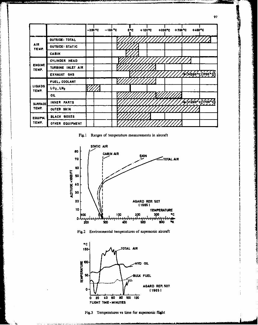
97

-20000C -100eC 06C +iO00C +2000C +3000 9C +00Cnfl -

OUTSIDE: TOTALAIR _______________________ ________ _________ _________ _________

TEP OUTSIDE; STATIC

CA BINK

ENIE TURBINE INLET AIR

TEMP. (va

FUEL, COOLANT ___ _______

LIQUIDS L0LNrONTEMP.

3U~F INNER PARTS 0C104

TEMP. OUTER SKIN_

EUP.BLACK BOXESt

EOUIP I I

TEMP. OTHER EQUIPMENT

Fig. 1 Ranges of temperature measurements in aircraft .

gaoa70~ -- OA I

20 AGR REP050

00 1 200 '*'C0'

2 00 5010 60 '

Fig.2 Environmental temperatures of supersonic aircraft

'C

IS0- _TOTALAIR

_.-HYD OIL

a. 50.,-BULK~ FUEL

AGARD REP. 5070- 119651

0 20 40 60 SO 100 120FUIGHT TIME -MINUTES

Fig.3 Temperatures vs time for supersonic fight

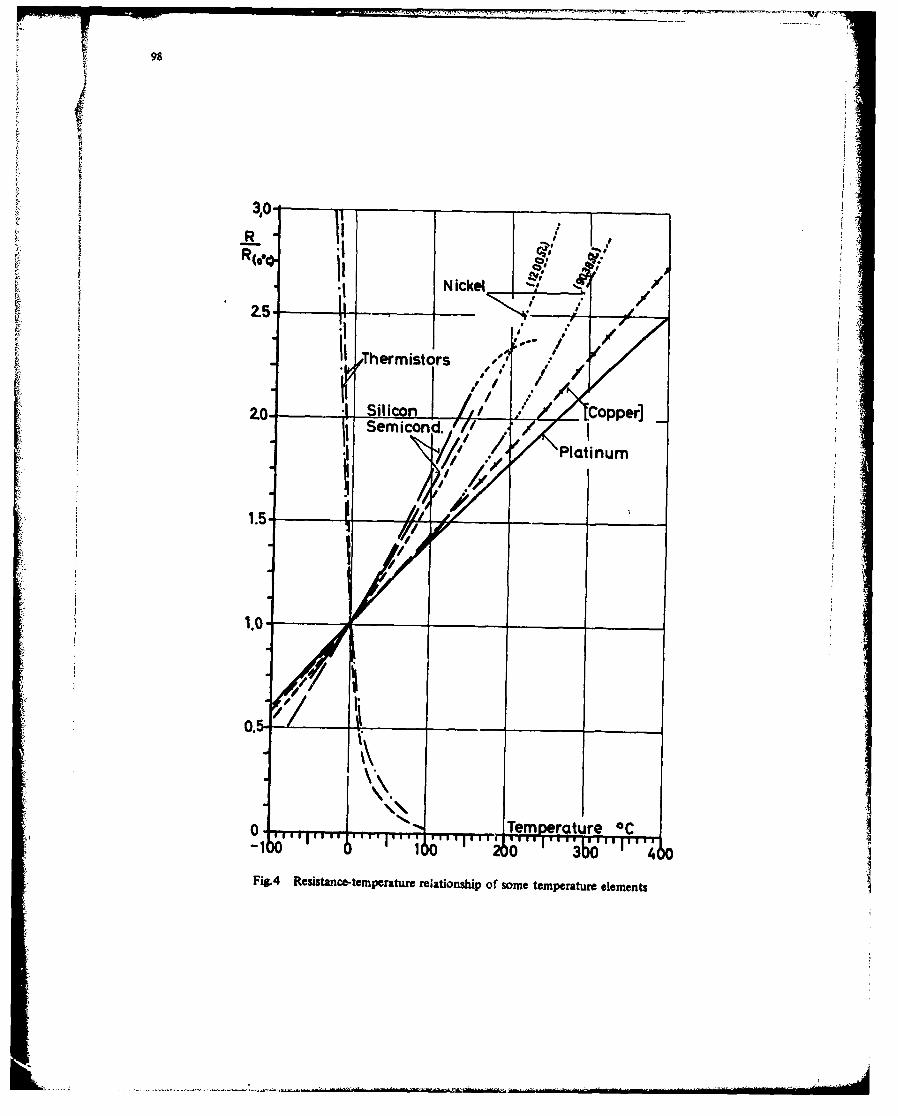
98

ip3,0-

RR(0 4

IThermistors

Semi~cond.

1.5-A

I~~Temrnte rot

V I

Fi8.4 Resistance-temperature relationship of some temperature elements

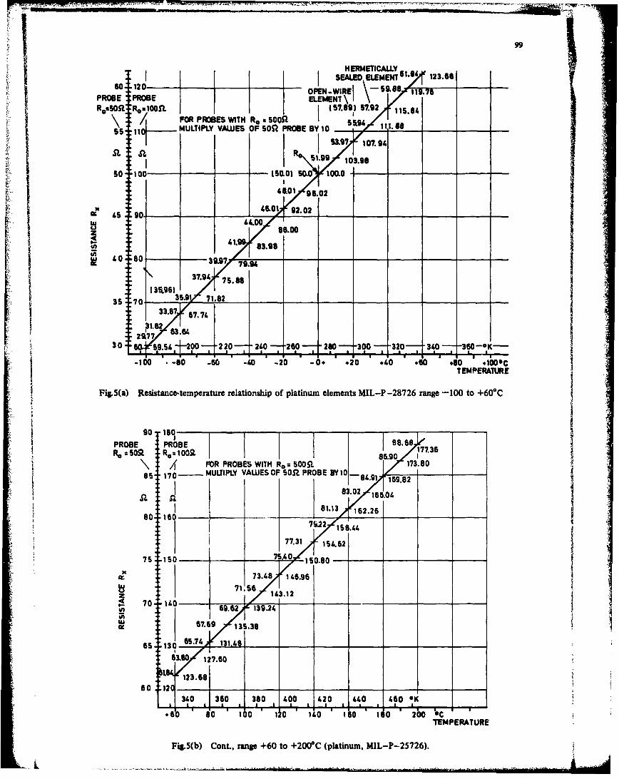
99-- HERMETICALLY

I____ ___ I......... __ J SEAUI LED 123.4Sso.• 1120'e' Sao$"120 " oPEN-WIRE \--:. ,

PROBE PROSE ELEMENT\I \ IIR0-50SSRo:I .OOf (57.09) s7.92 IIs.e0

/ FOR PROBES WITH R. 500o I""5';] MULTIPLY VAWES OF PROSE BY 10 S 1.

so 100-- -(S0L)50.0 100.0

45. 902 .0

640 6.00

40 180ý,, '003

II3S. .70- 35-912 71.82 ___ ______

30 59.54 00 PO 220-2,140 260 260 -300 32 10 3G0-

-100 4 -S0 -60 -, -20 -0 * .20 .1.0 .60 .50 100O*CTEMPERATURE

Fig.5(a) Resistance-temperature relationship of platinum elements MIL-P-28726 range -100 to +60°C

90189 6•17

PROBE PROBE 88Ro =505 Ro:t00Ik177.36 , 86.90 I\• 4 FOR PROBES WITH R0 : 5Q0.9 173.80

85 170- MULTIPLY VALUESOF 50.• PROBE BYVIO 9 .85'" 10 • 8• 1 169.82

183.02 166.0480 ______ 81.13 ~~162.26I___ ______

76.22

77.31I 154.6

75 50____ 75~.&.0 150.50-

773.48 146.9671.56 113.12

4 70 140 69.62 139.24

.67.691 - 13S.36

65 130 65.74Y l31,/.8

63.90 127.60

S123.61 860 12_ 1

3o0 360 380 1.00 1.20 .1.0 1.60 *KSIi i o IbOl l I o lb

o 8 1 10 11.0 160 1 0 2 UCTEMPERATURE

FiB.5(b) Cont, range +60 to +200*C (platinum, MIL-P-25726).

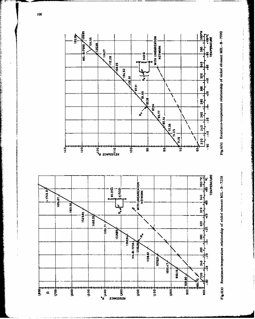
100

*0 o

* 0"

4' AA

"" no C '04

NN

____t 00__

y~~~~~ M___ __________

*A10

II10 AU

la C2

a0.,

0

C4C

040

0~0 0 0* a 0 0. 0 0a

-- CXs 33wNsisI3a ,

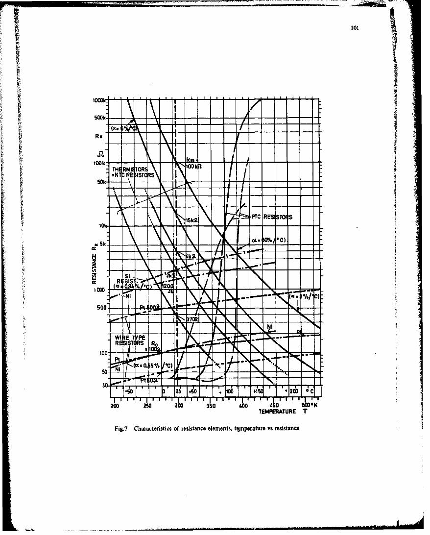
101 l

S4k

100k---.- - -

~ S?1 THERMIST10k -

5 NI RE IST( RS I- -- -

PTC RES! STOS

-i - %- -k

Ix R SISTFig. Chrcei0c frssac lmns eprtr srssac

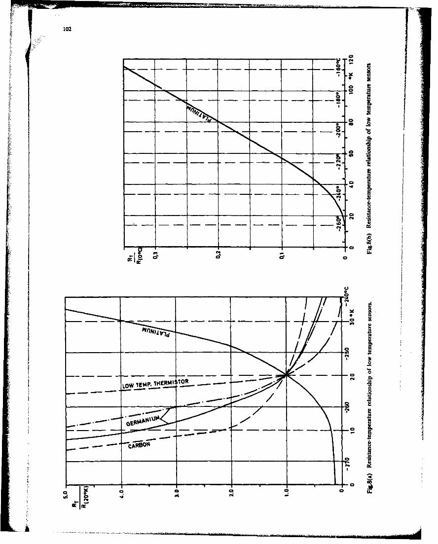
102

______

00

_ CD

C4A

C!U

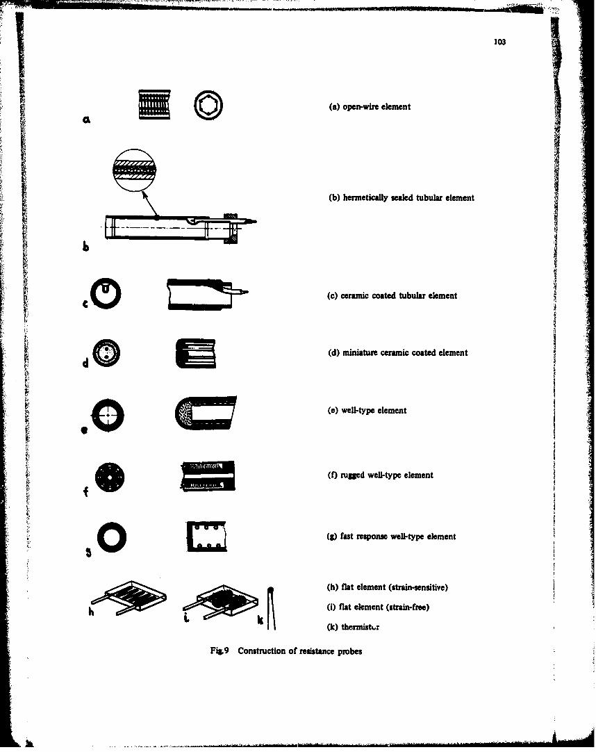
103

(a) open-wire element

6 (b) hermetically sealed tubular element

(c) ceramic coated tubular element

(d) miniature ceramic coated element

(e) well-type element

(f) rugged well-type element

(g) fast response well-type element

()flat element (strain-sensitive)

(i) flat element (strain-free)

(k) thermist.,r

Fi&.9 Construction of resistance probes

AL

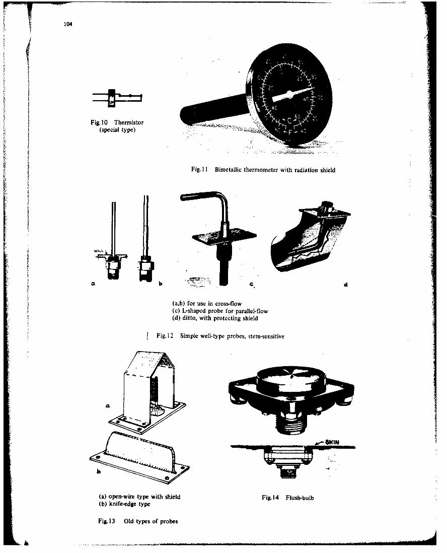
II

Fig. 10 Thermistor(special type)

Fig. II Bimetallic thermometer with radiation shield

1V

WAAM

a b- d

(a,b) for use in cross-flow(c) L-shaped probe for parallel-flow(d) ditto, with protecting shield

Fig. 12 Simple well-type probes, stem-sensitive

(a) open-wire type with shield Fig, 14 Flush-bulb(b) knife-edge type

Fig. 13 Old types of probes

&k

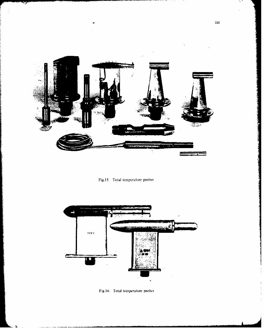
4-4

Fig. 16 Total temnperature probes

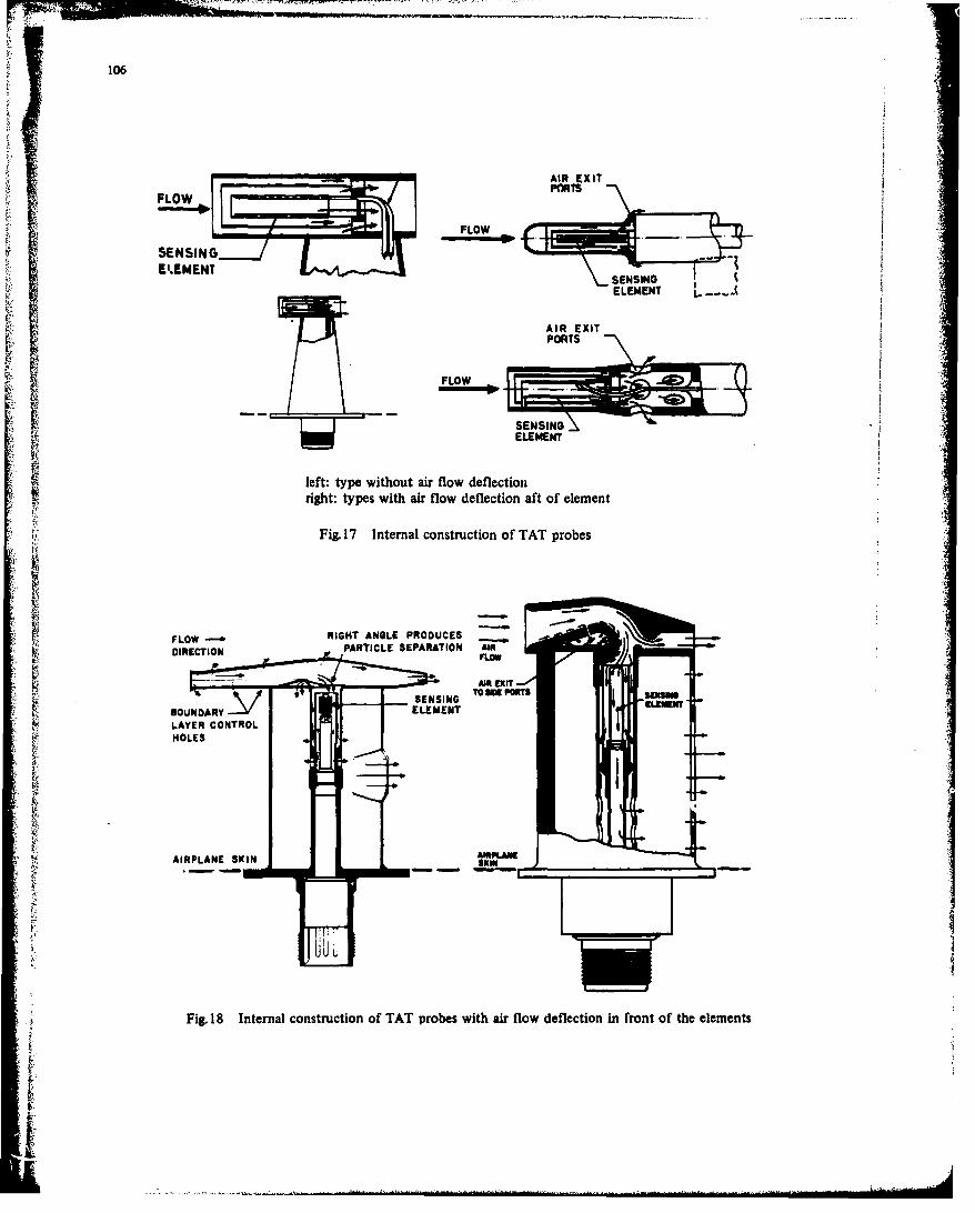
106

FLLOW

4 FLOW:

PARTICLEMEN SEAAILLf

FLOW

LAYERECONTRO

~~~~~Fig. 18 Internal construction of TAT probeswiharfodelconifotofhelmns

RIH NLEPOUE

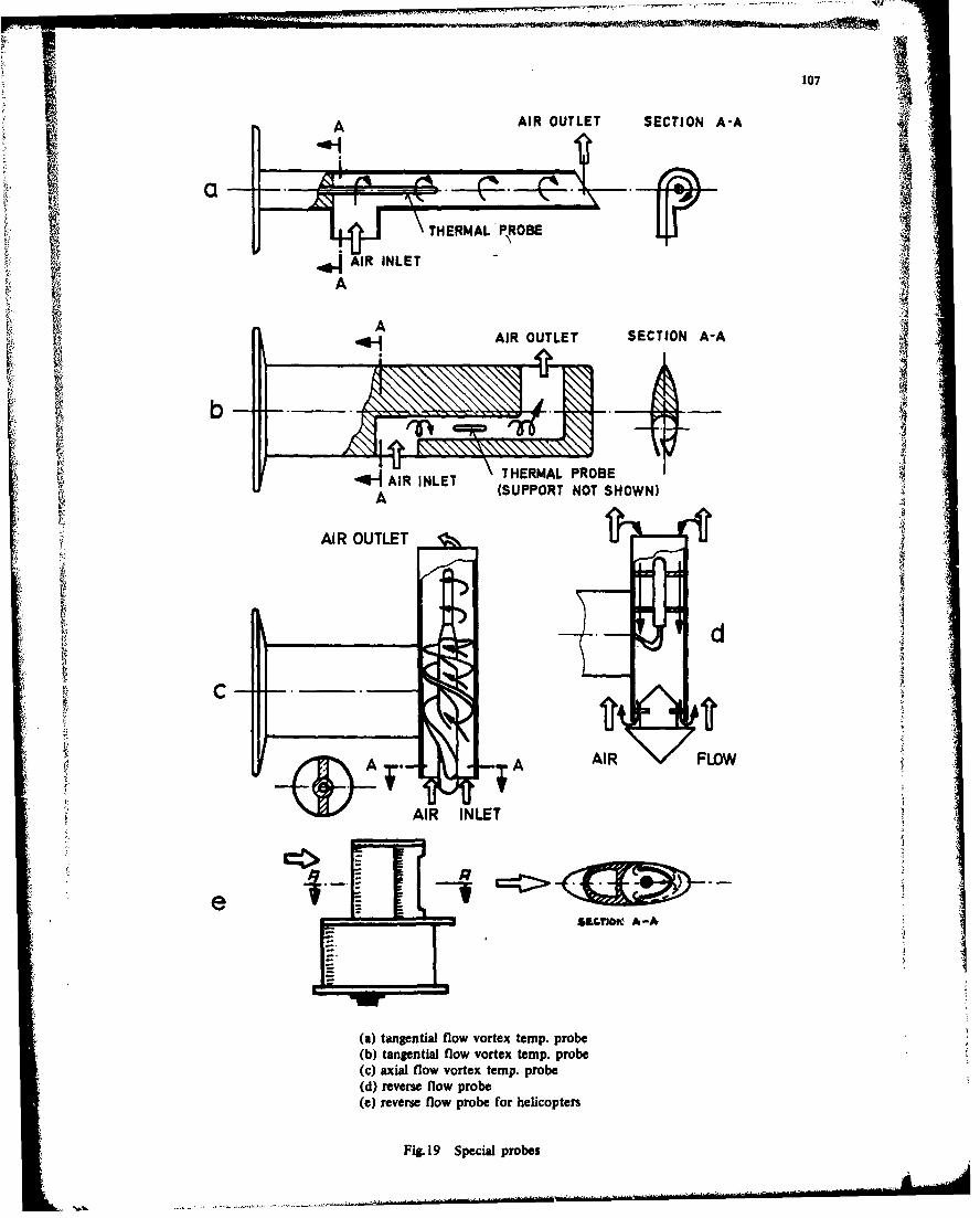
107

AAIR OUTLET SECTION A-A

*T VA

AAIR OUTLET SECTION A-A

.4AuRINLET THERMAL PROBE4A"A(SUPPORT NOT SHOWN)

AIR OUTLET

AAIR FLOW

AIR INLET

(a) tangential flow vortex temp. probe(b) tangential flow vortex temp. probe(c) axial flow vortex temp. probe(d) reverse flow probe(e) reverse flow probe for helicopters

Fig. 19 Special probes

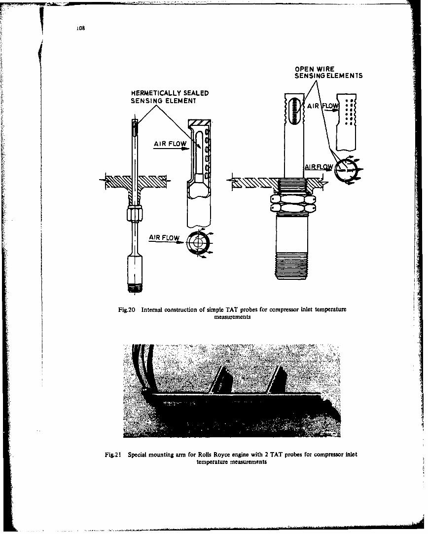
OPEN WIRESENSINGELEMENTS

HERMETICALLY SEALEDSENSING ELEMENT ARt

AIRA

(A I FO

* Fig.20 Internal construction of simple TAT probes for compressor inlet temperaturemeasurements

. ... -....... ..

4i 1'.]~

Fig.2 1 Special mounting arm for Rolls Royce engine with 2 TAT probes for compressor inlettemperature measurements

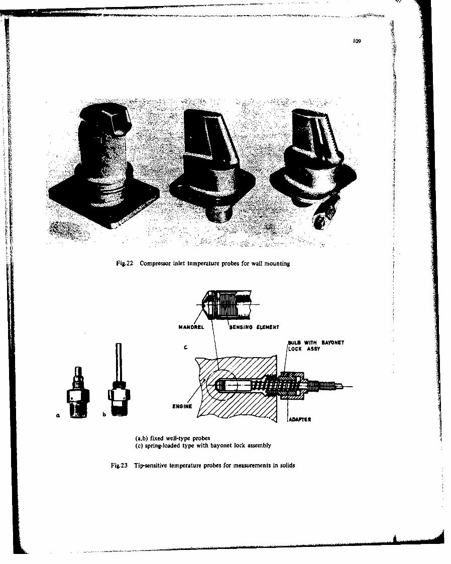
109

P 4

Fig. 22 Compressor inlet temperature probes for wall mounting

MANDREL SENSING ELEMENT

C BULB WITH BAYONET

(a,b) fixed well-type probes(c) spring-loaded type with bayonet lock assembly

Fig.23 Tip-sensitive temperature probes for measurements in solids

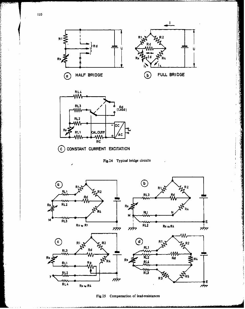
110

R1 RRRI

RRd

Rxx

HALF BRIDGE FULL BRIDGE

ROC

RRL3

R3 R

Fig2 Copestin fled-eisane

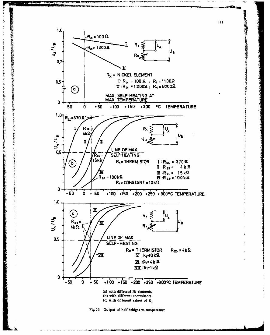
111

1.0. 100 St

Rx ~ 7j0.7-

Rx = NICKEL ELEMENTP0.(5" 1: Re a100. A RI=110051J.

.. L, Q ti: Ra = 1 2002 ; Ri =4.000A.

MAX. SELF-HEATING ATI .MAX. TEaMPERATURE

50 0 *50 +100 +150 +200 OC TEMPERATURE

R mc

a Ii,, •LINE OF MAX.

(X5 -R 26= SELF-HEATING iI-50 Rx= THERMISTOR I :Ris = 3705t

B :Rs = 4k.,R"I:R 2L= 15kS,

.Rzs=100kSZ I!:R %6 100 kS.R4 = CONSTANT 10kdL

0'•-50 0+ 50 .100 +150 +200 .250 .3000C TEMPERATURE

1.0-

R1 -

SRe•= Ue

0.5 LINE OF MAXSELF-HEATING

Rx a THERMISTOR Rin 4k2-•/11 " • ":1R t-1 0 k •

MI :Rs4kit"MlT:Ri-l k2

0 ý '-50 0 *+50 .1 200C TEMPERATURE

(a) with different Ni elements(b) with different thermistors(c) with different values of R,

Fig.26 Output of half-bridges vs temperature

; ,S -

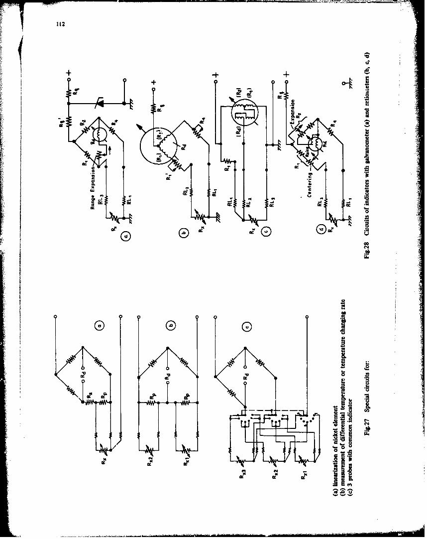
112

.0 •

aa

a:,4

-. J2

C ,V.

00Ke

bo

-00

*09 0

cc ce

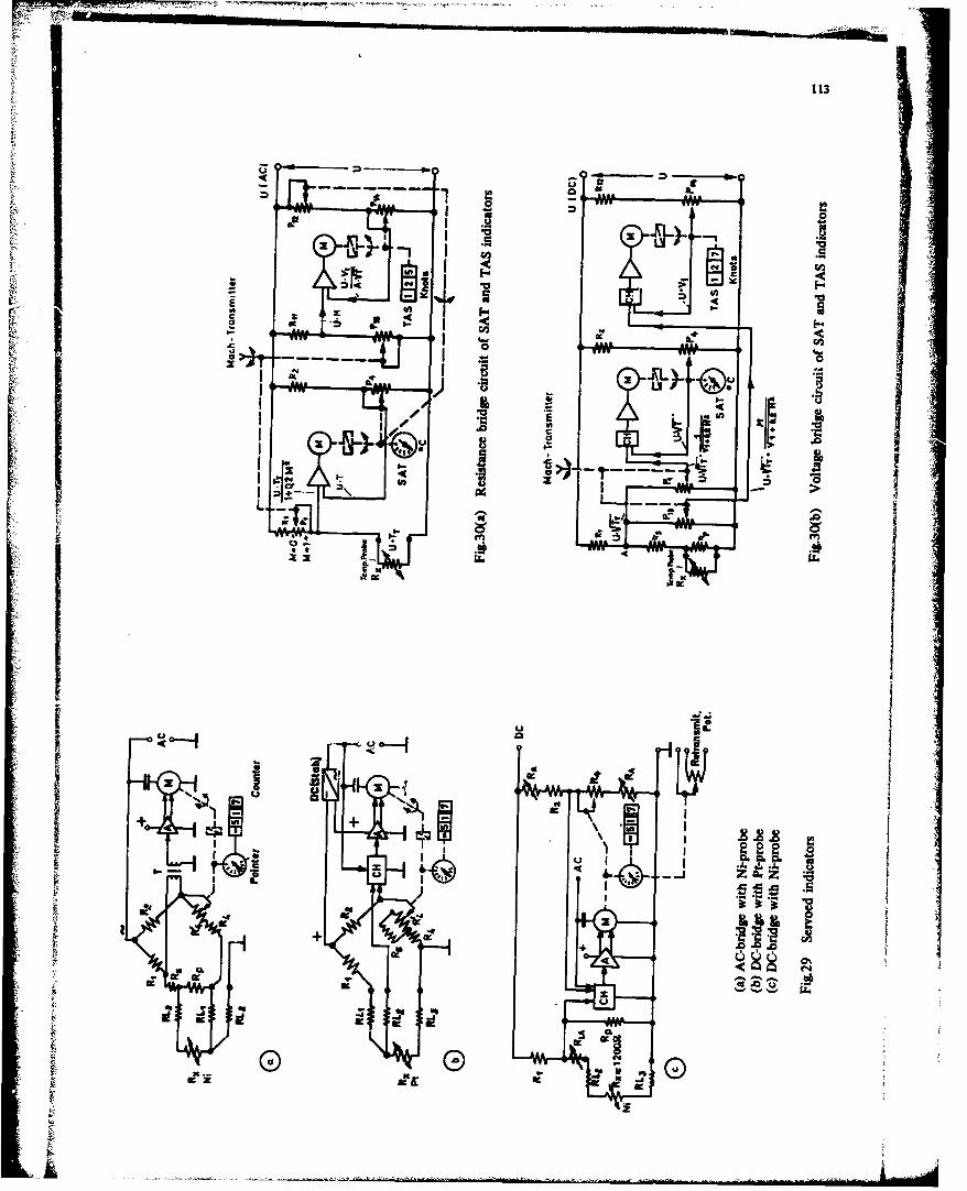
113

It ,,.... V` V- , l ilI ' 0

-I-. I AA- A

"I"it.

w -

-' ,. a,, ,

I- I

* K+ a -+

H i-- (f -

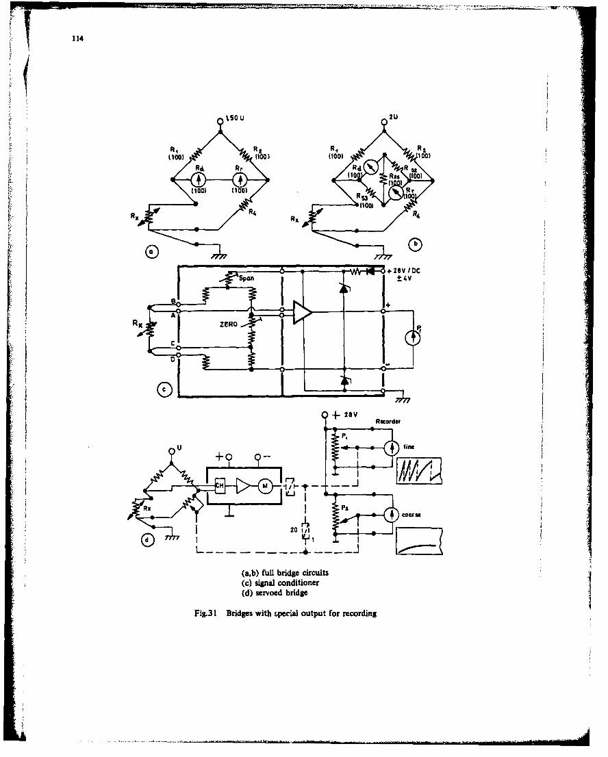
114

%so U2U

(too) (1001 00)i:R& Rr Rd

+ .25V I C

Z R 4-2-0

RP 4

J in

R RRcord

I U_ __in

Spa ®:t 1.I Pa

02 0,I

S(a~b) fuli bridge circuitsBI ; (c) signal conditioner

(d) servoed bridge

Fig.31 Bridges with specia output for recording

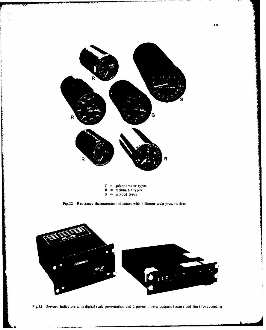
115

R R)

G = glvonnwtertypeR = rtionetertype

S? 0 seroe tye

Fig.32~ ~ ~ ~ ~~~~~1 Reitac throee"niatr'ihdfeen l rsnAtin

Fig.3 Srvod idictor wih dgitl salepreenttio an 2 otetioete ouput (cars an fie) or ecodin

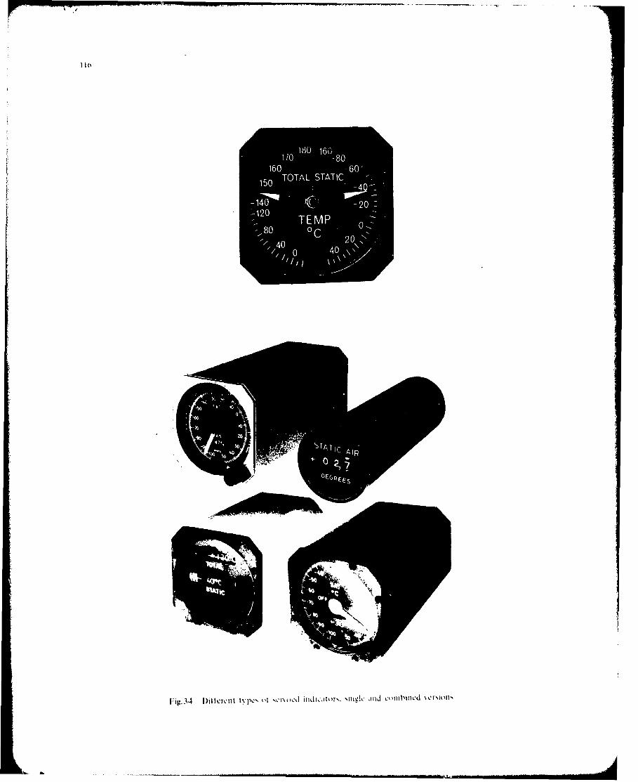
110 -8

15 TOA SAI

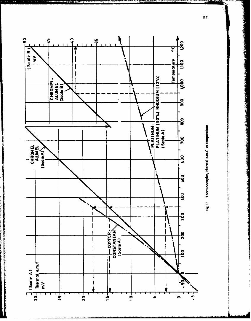
117

Sn 2 0

W Eu

04

OS 0

op lk

00 l

_ _ "K>CD4'

_ _ VIC3* I I I I

t~'4 -

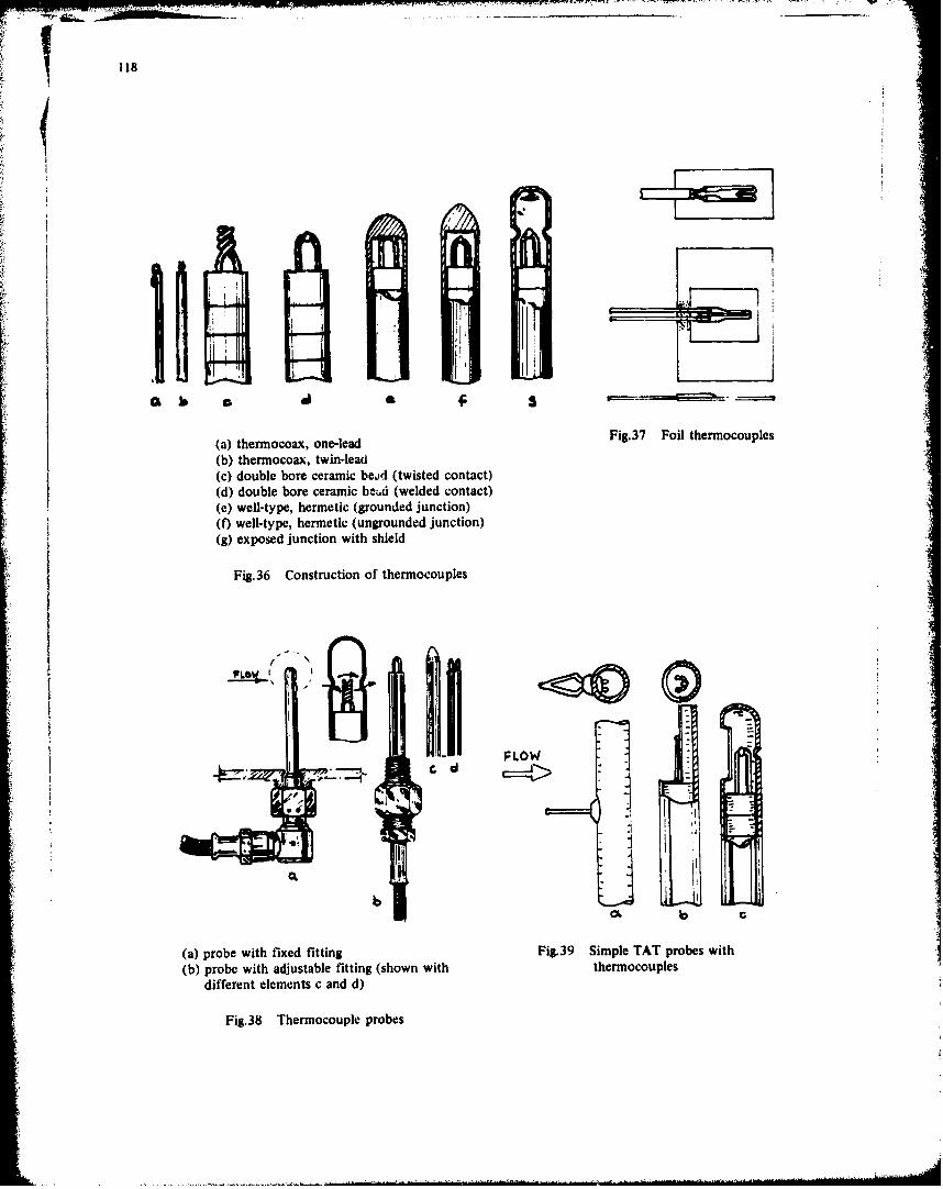
118

f)

(a) thermocoax, one-lead F,7Fi hroope

(b) thermocoax, twin-lead(c) double bore ceramic be..d (twisted contact)(d) double bore ceramic beud (welded contact)(e) well-type, hermetic (grounded junction)(f) well-type, hermetic (ungrounded junction)(g) exposed junction with shield

Fig.36 Construction of thermocouples

- FLOW

1QI

ab , d

(a) probe with fixed fitting Fig.39 Simple TAT probes with(b) probe with adjustable fitting (shown with thermocouples

different elements c and d)

Fig.38 Thermocouple probes

FLO

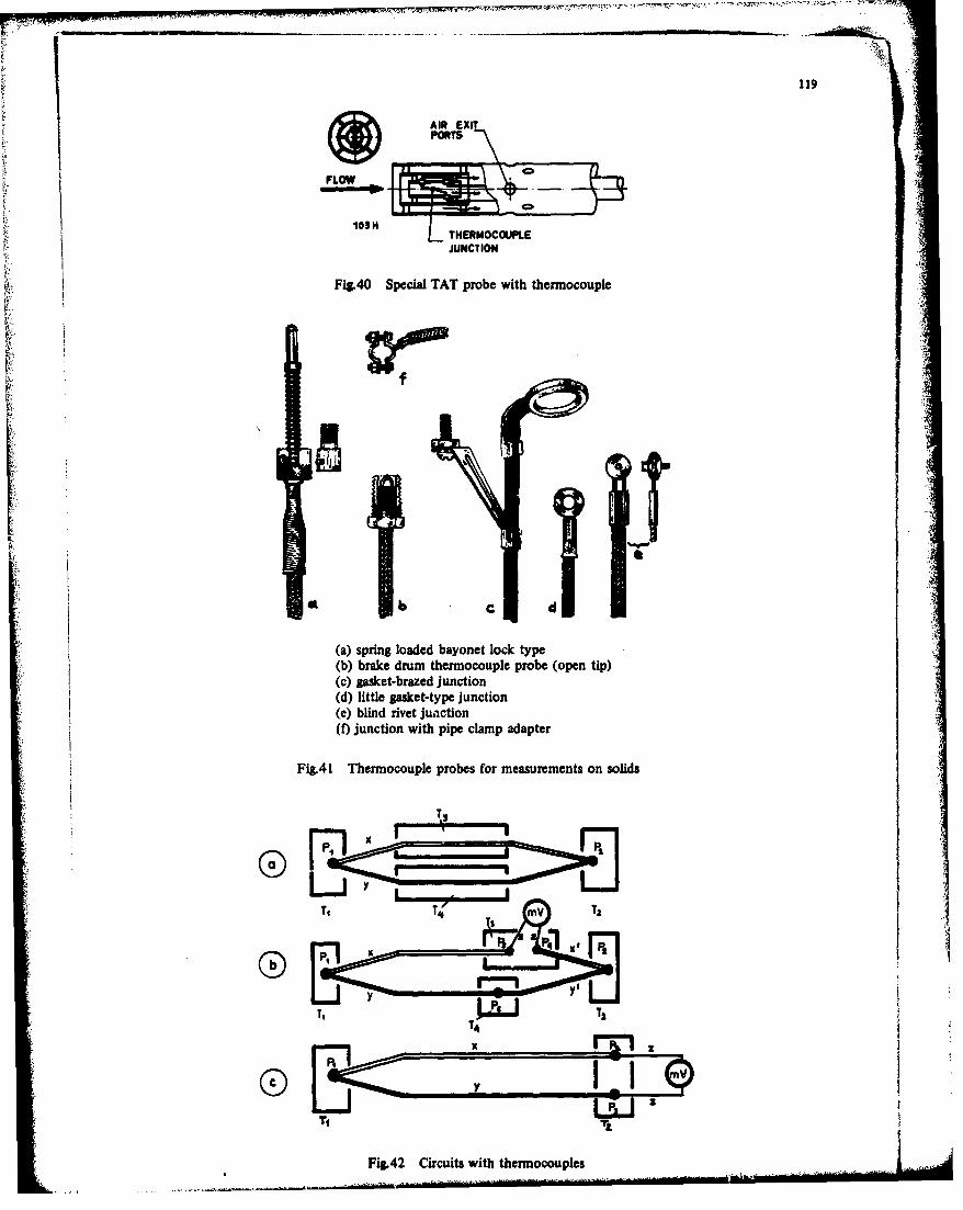
119

AIR EXIT

FLOW 10o3rH

10!1H -- TERMOCOUPLEr

JUNCTION

Fi&40 Special TAT probe with thermocouple

bt C

(a) spring loaded bayonet lock type(b) brake drum thermocouple probe (open tip)(c) gasket-brazed junction(d) little gasket-type junctionWe) blind rivet junction(f) junction with pipe clamp adapter

Fig.41 Thermocouple probes for measurements on solids

•;T1 T1" MV TS

P.1, ,'L.I

"" •o

Fig.42 Circuits with thermocouples

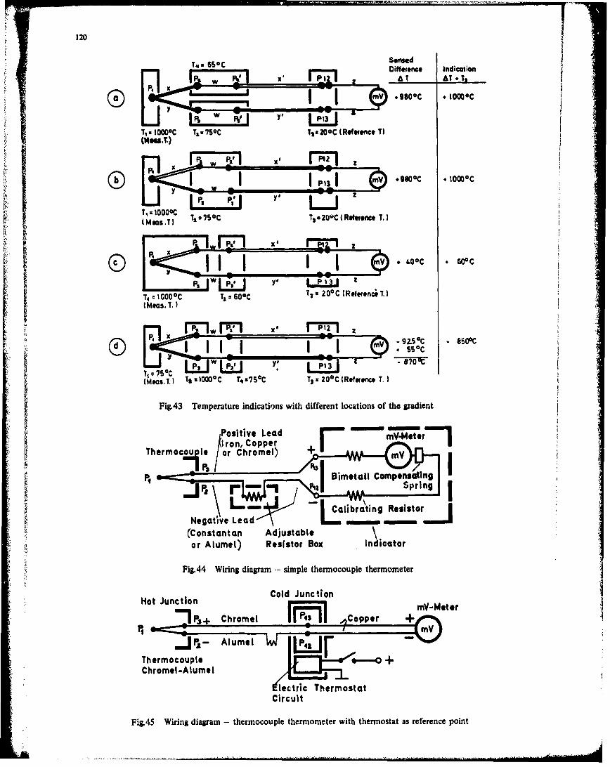
120

'! T• 650(;Sensed

Diffrence Indicationiw I X' A TATT *TT._

IP31mV 2600C 10000C

Tiu aI000C Tgo 7SOC TI,2OOC (Refetonce T)(14f..T.)

• a w _--o"-o"

rIOGOOC*2 0 C OO O

T•:1000o

(MgOs.T) T A 750 C Ts 200C tRefgence T.

I~m. , ),.(:D 4 ,; ' : -i•ic mV$ "9"*+S°C "8C"

T P-, ? oC

T .1000 0C TA 600C T,: 200 C (Reference TI.(Maoos. 1.

SFig.43 Temperature indications with different locations of the gradient

I ,~~~~~Positive Lead -- m' tr l

I hl~ron, Coppe~r .|

P !* P13 870

! • I__"_:_"•J• -- I Calib'rating\ Resistor INegat ive Lead .---...

(•Constantan Adjustable\-• ,.or Alumet) Resistor Box Indicator

•- ~Fig.44 Wiring diagram -- simple thermocouple thermometer

Hot Junction ClJucin mY-Meter•, ,,•nP,- Chromel ,Copper +-

Thermocouple ---ehr--.-O -A

Electric ThermostatCircuit

Fig.45 Wiring diagram - thermocouple thermometer with thermostat as reference point

Wa r

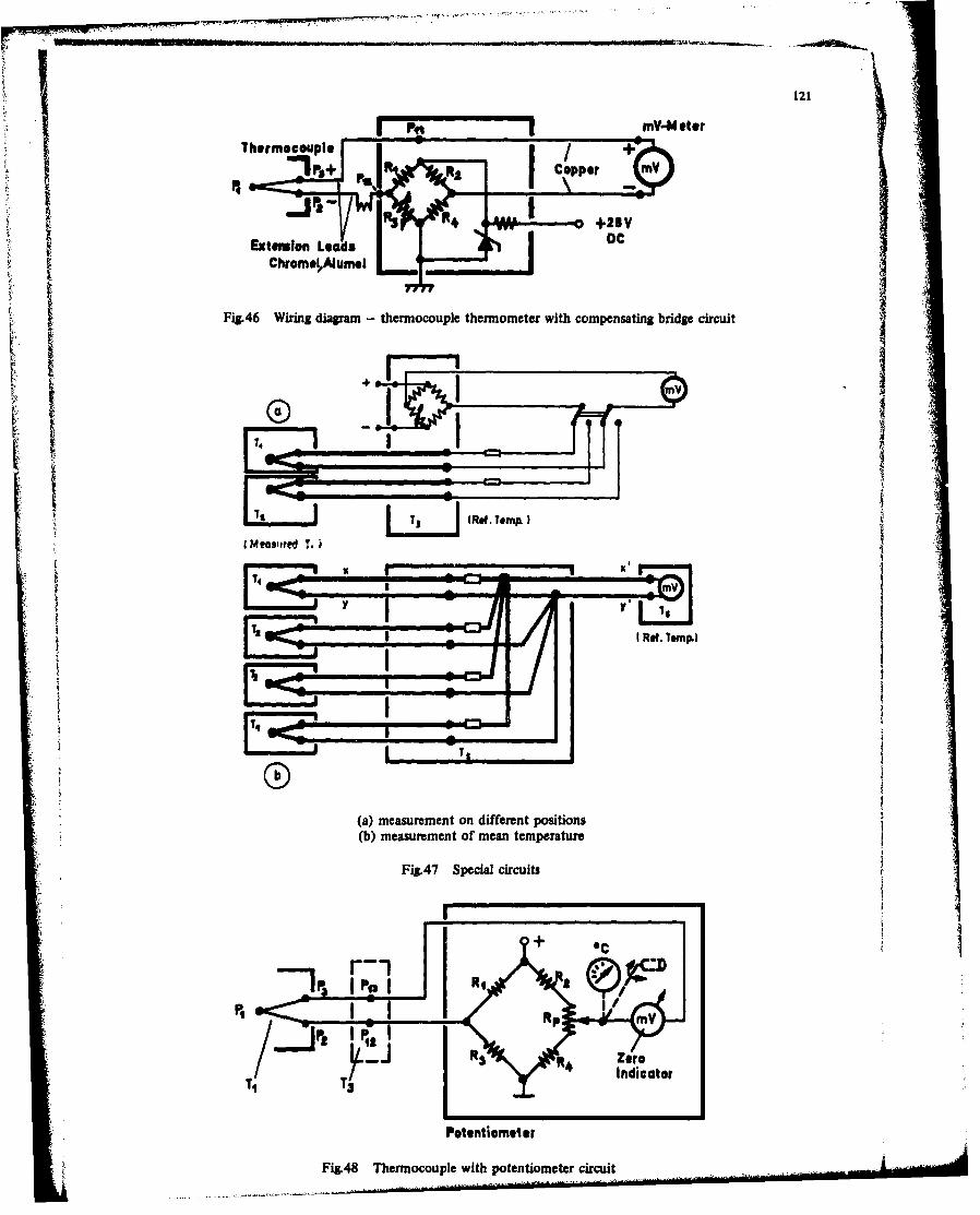
:1 121mnV-etier

Thermocouple

vvq111 0+28VExt Ion Leod s

ChromelAlumsI

Fig.46 Wiring diagram - thermocouple thermometer with compensating bridge circuit

j S (RefT, mptl

(MT4~e T

(a) measurement on different positions(b) measurement of mean temperature

Fig.47 Special circuits

R <

Rp pm

T3

Fig. 48 Thermocouple with potentiometer circuit

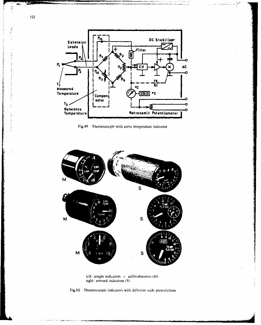
122

F"o7 DC Stabiijzer

Leaseds'

RefF [tercTempeatur RetaitPtnioee2

Fi.9 Temcul ihsev3eprtr niao

fp C M A

P, '

rig t: s roe i0iaor

Fig.4O Thermocouple idctr with se iofemeratusrae i sndi ations

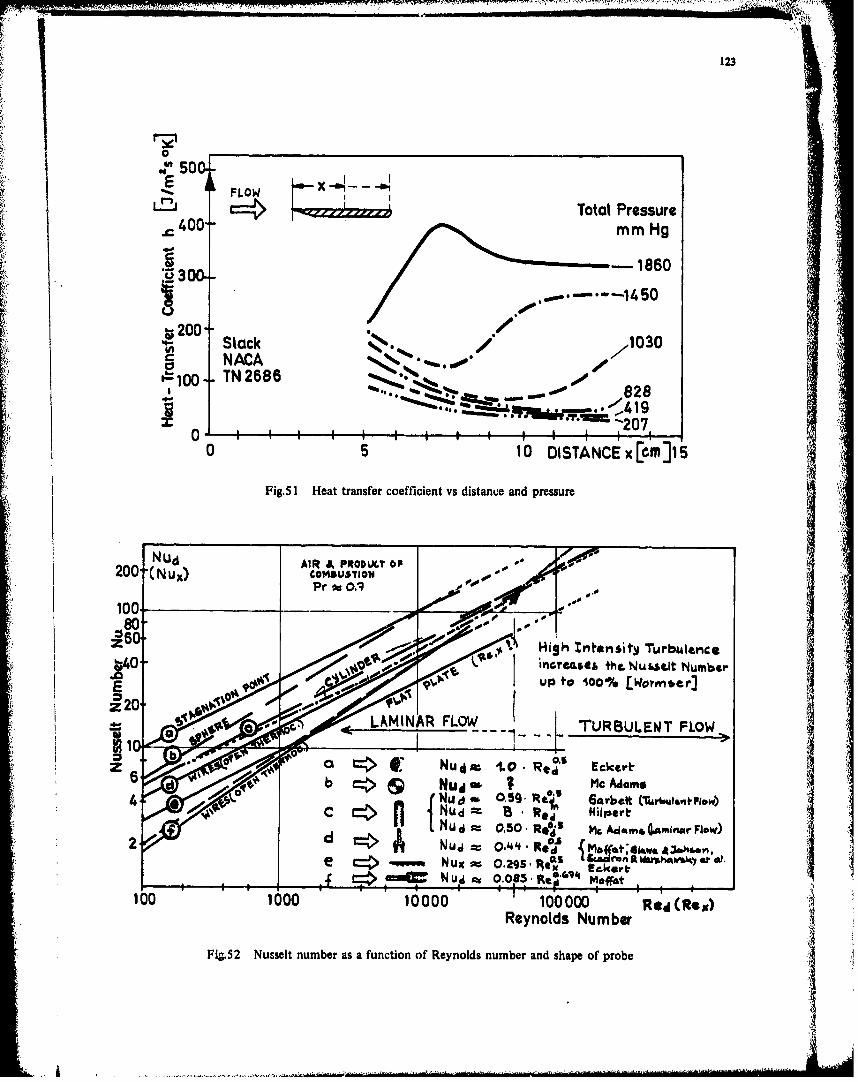
123 -

50E 50

E FLOWL2J Total Pressure

~400mmH

V200- Slack 1030NACA q

100o TN 2686elm mono828 <419

~2070 I III I I0 5 10 DISTANCE x[Cm]15

Fig. 5 1 Heat transfer coefficient vs distance and pressure

nCO56 1u0eI Numbir0

200--(ux) cmpM$7010m'6 ~ ~ P dg 01 ( u10 e ~k

e'rr~t +he Nugel Number¶~ II~~

R pynolds o NumbrrnbrEi.2 Nsetnme safnto fRyod ubradsaeo rb

A . . . . .. '. j..

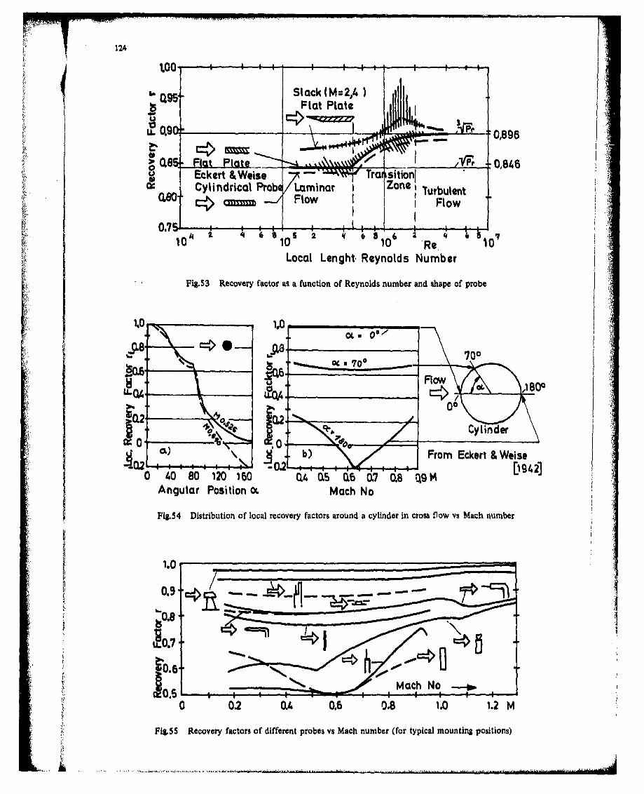
13a9 Stack (M:-2,4)

Flat Plote

0,9

U Eckert &Weise -Tra si0,89

~:eoCylinridcal ProbeLaminar I Zone Lrrbr7

0.76 5~.

-0.2- . 0 010 0 1hQ 6 07 0.8 D90

Local oitono acght RenolsNme

Fig.54 DsRiuinolcarecovery factora s a rfnt o un d af eyn lisndmer ind crshap ofo proa ube r

1.0__ __ __ __ __ __ ___ __ __ __ __ ___.0_

~~700Mah0o0.-

i a a a0 0.2 h 0.60.8 101802

Pig55 ecoeryfacorsofdiferet pobe vsMah nmbe (fr tpicl ouniipstos

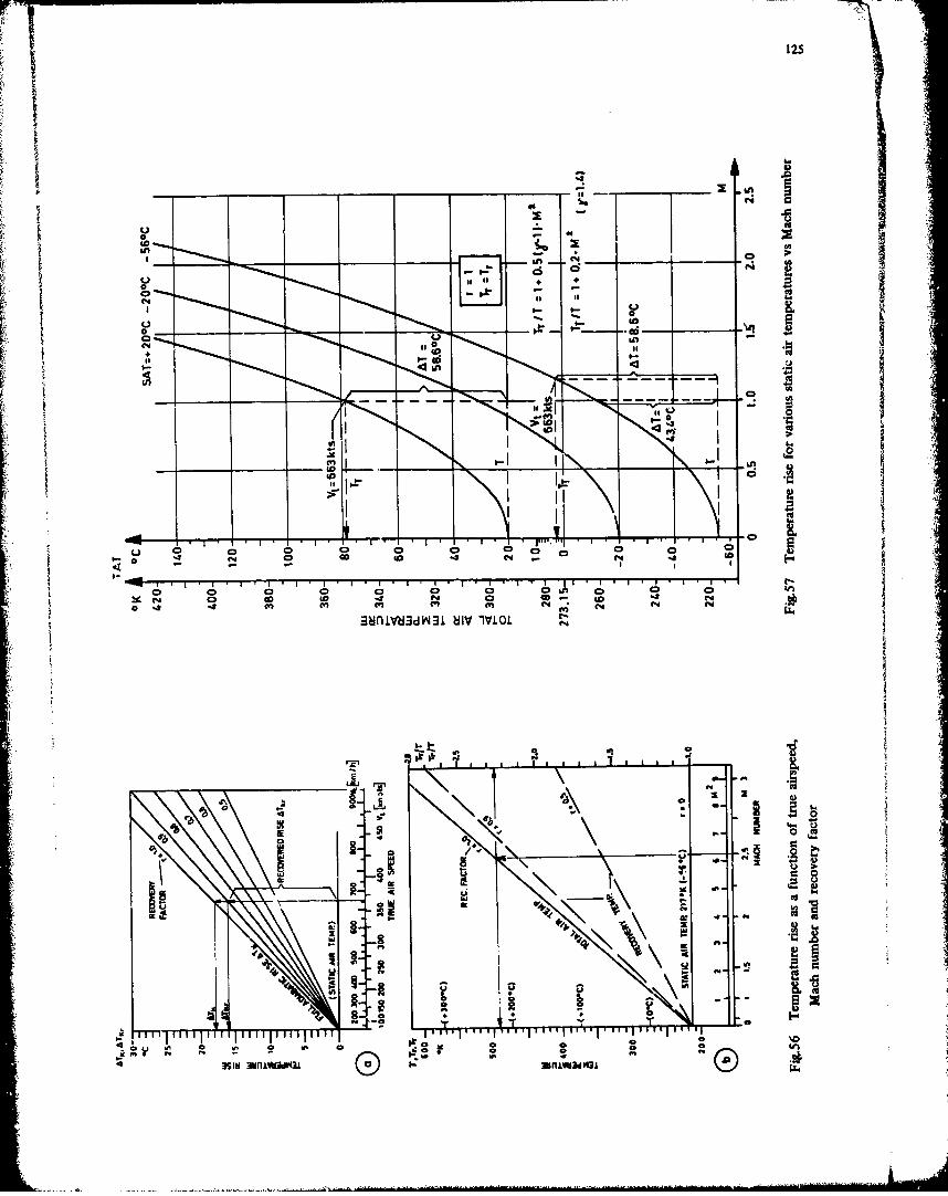
125

.4 N4- -

CS d

40 0 I

coo

In

Lai

-F-U-

4 Ol 0C v 0 a 3N 0 00

0 ~ ~ 31 301* rI36P N * 0

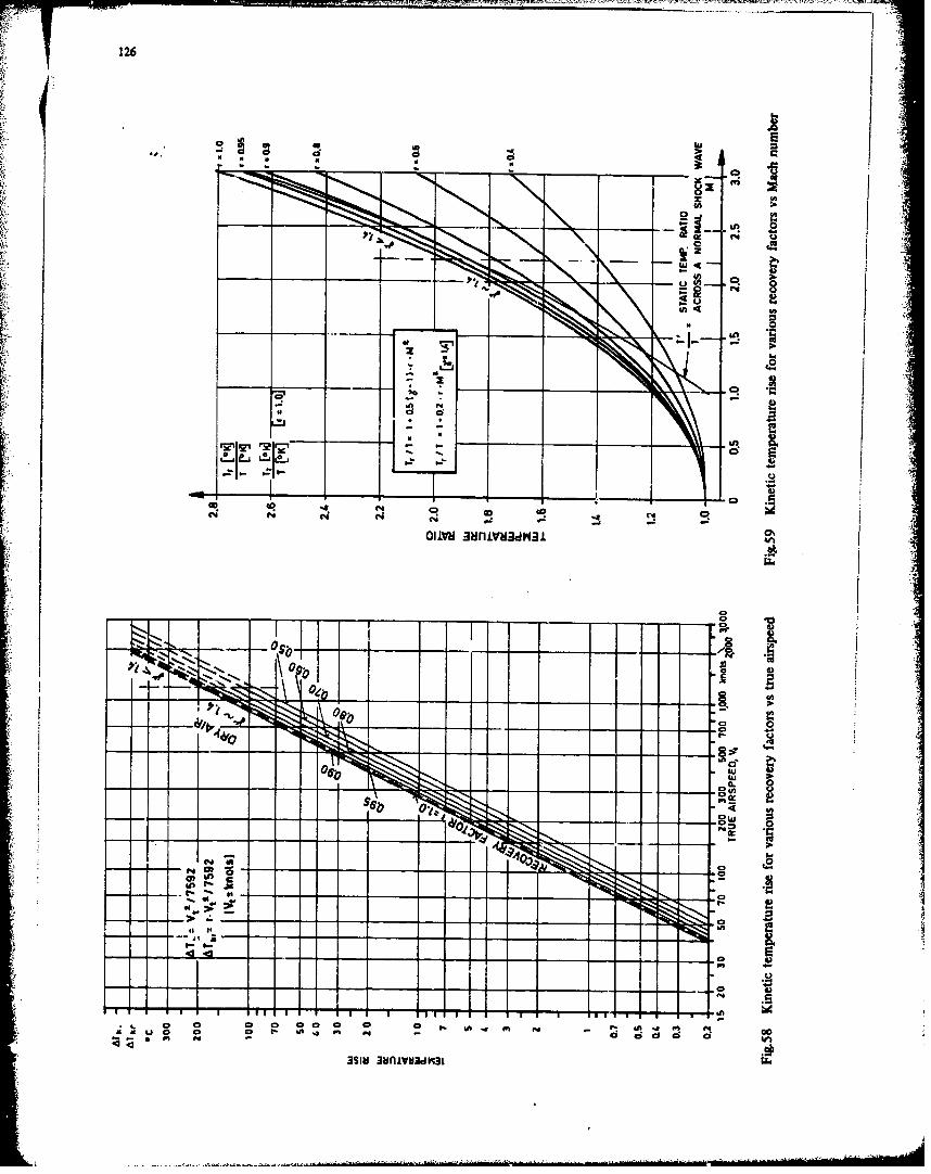
126

N - -t -9

J8..

da

ZIIFF-

- b-

- f'~ a ad 4 Cq C4 40

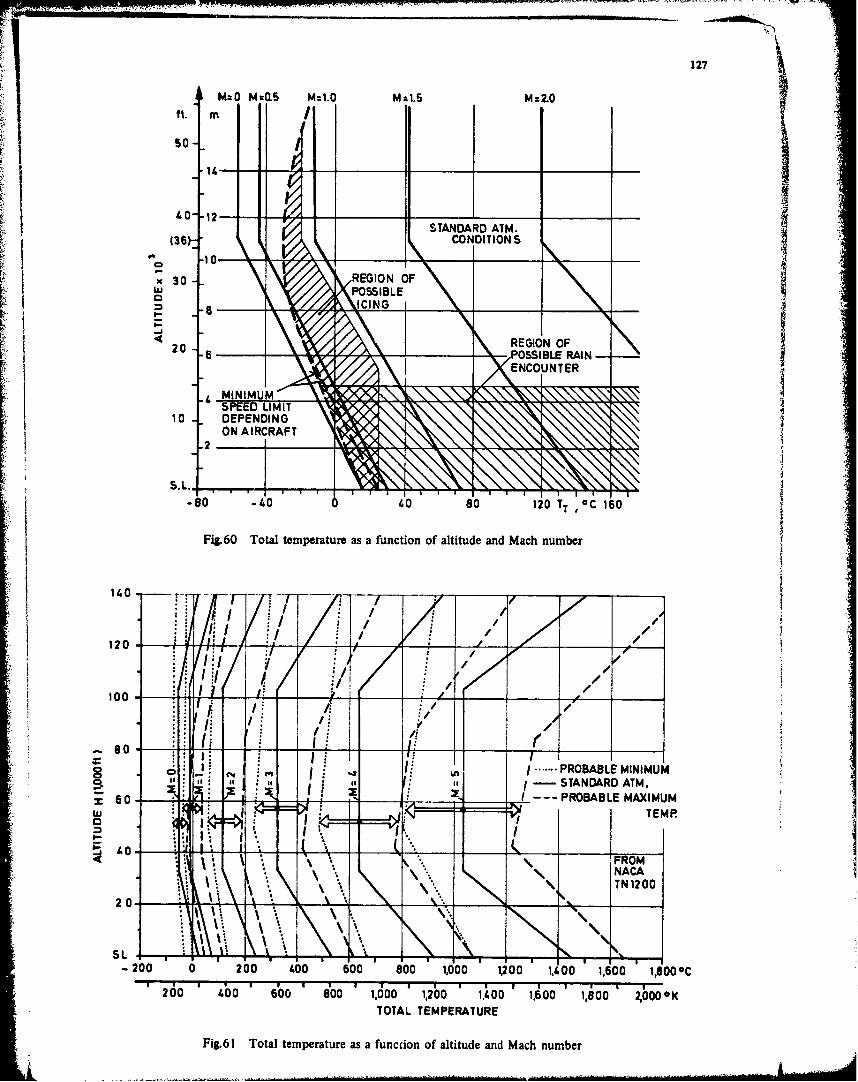
127

M-O Mz0.5 M:1.0 M21.5 M:2.0ft.m/

10

-x 30 REGEGON OFF

S20P-6PSBLE

1 . DEPENDINGONREGIONAFF

-20

£. 8 -, 0 80 120 TT ,0 C 160

Fig.60 Total temperature as a function of altitude and Mach number

6I0 - - POSIL RAI

1 1 0 /

! 120o • / ," I/

SP .E L /-

-8 o4 I)4 o10T ~ 6

:10

a:.. .... ROAL MINMULai" , - STANDARD ATM.

•50 .IZ _ --- PROBABLE MAXIMUM

60 - I I..

-J __ __ FROMNACA

\.z...\*...TN120020 -\*

" 'i

SL,- 200 0 200 400 600 800 1,000 1,200 1,400 1,600 1,800 0 C

200 * ,00 600 , 800 1.000 1,200 , 1,100, 1.A00 1,00 , 4000 1KTOTAL TEMPERATURE

Fig.61 Total temperature as a function of altitude and Mach number

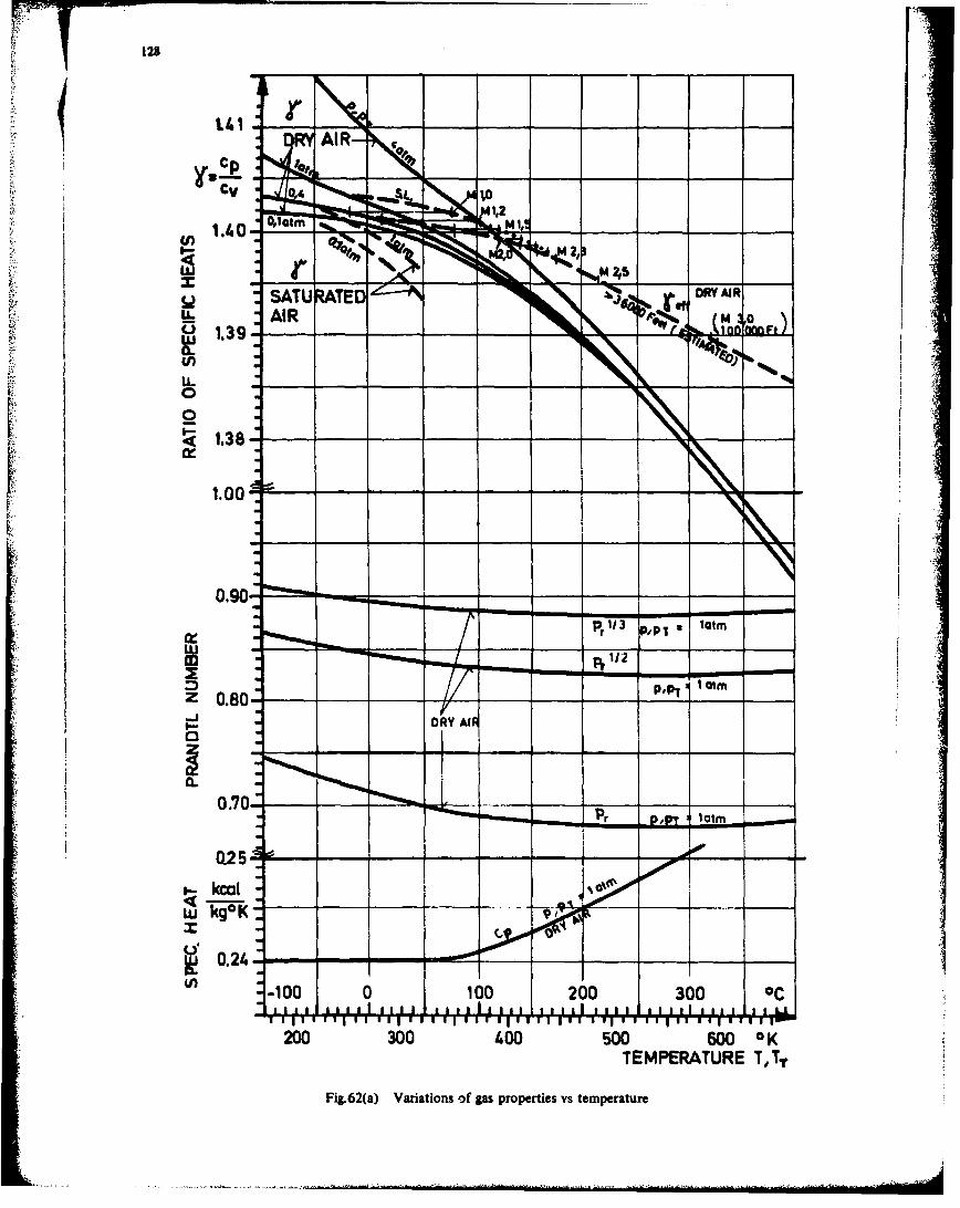
<V128

AIRAI

C.)

(n1

1.39

LiL

0

1.00030

2000.60 0

TEM3PERAUR ltTFir.(a Varaton o7 gspoetesv eprtr

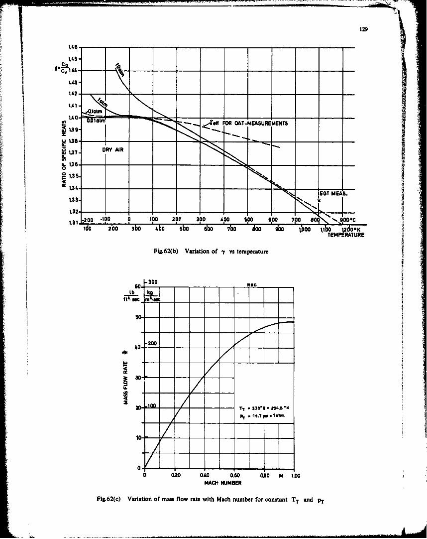
129

tlA -- _ _ _--

1.( 5

lAt

ONm FOR OET-MEASURTMENES

1.32- --- _ x

02-O1.31 200 .100 0 100 200 300 400 %00 600o 700 800 ý 90*

do 2'00 30o i-0 0o 600 700 00o 900 1000 1100o %2 0*KTEMPERATURE

Fig.62(b) Variation of y, vs temperature

200W-"

30/- - - "S1* -Z4S"

30'

0 0.20 O0O 0.60 080 M 1.00MACH NUMBER

Fig.62(c) Variation of mass flow rate with Mach number for constant TT and PT

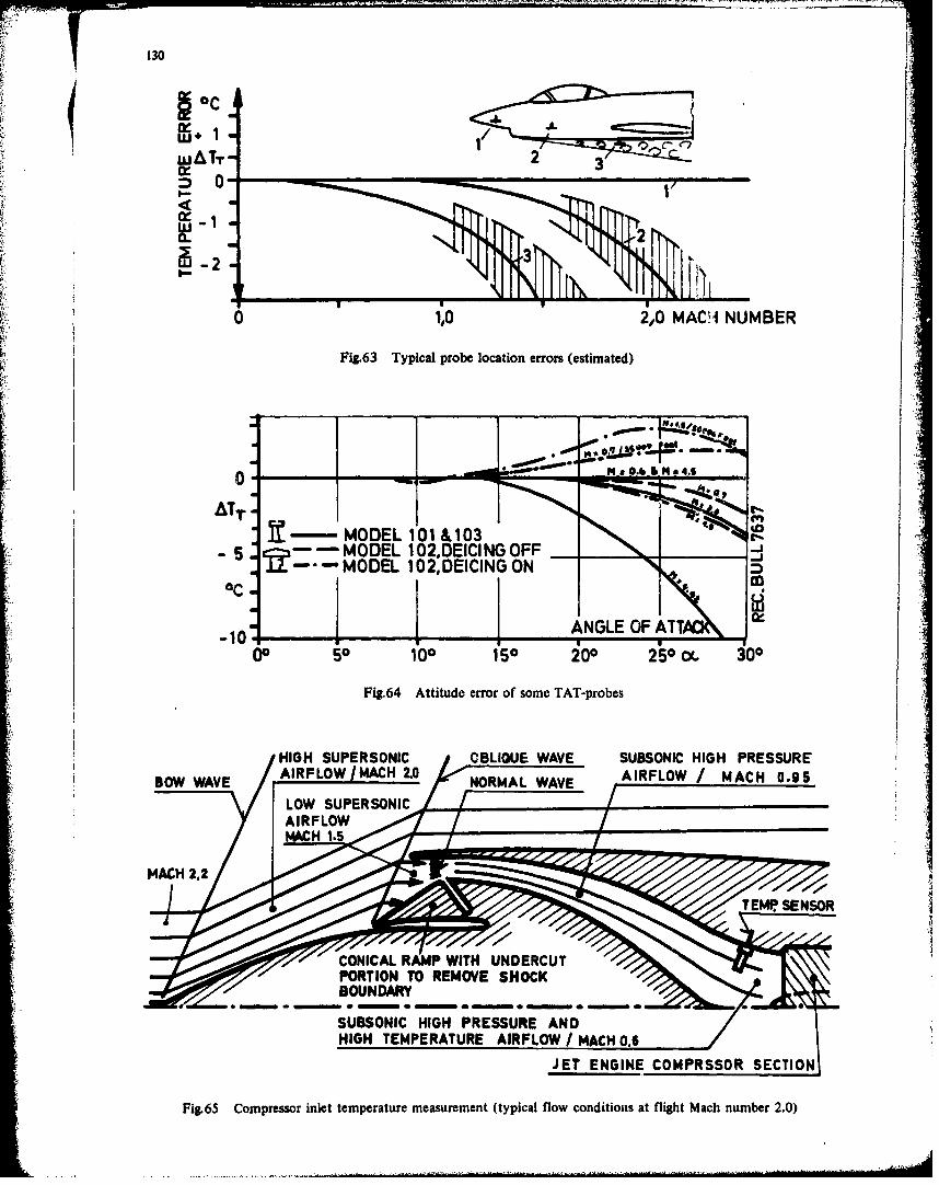
130

0C.

0*-

-T2

0 1',0 M0DEL 102DENUMNER

Fig.6 ATtpitudproelcto errorof so(estiatpoes)

HIGH~~~~~~~~H SUPRSNI &MeOU WAE SBONCHG PESRA0 FO/AH20 NRA WV IFO AH09

SUSNI IH RSUR N

JE-ODE ENGIE COPRSSRSETIO

Fig65 omresor nlt tmpeatre easreent(tyicl fow onitins t ligt Mchnumert .0

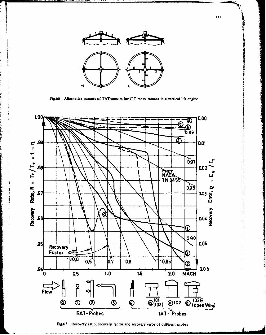
131

Fig.66 Alternative mounts of TAT-sensors for CIT measurement in a vertical lift engine

to 00

0.02w

w

1.9505Recovery

Factor~

0.0 6

Flow

(9 ( () ) (D @'101' 02( 10 2E_ _ _ _ _ _ _ _ _ _ _ _ S( 3 0 1 0 -o p e n W i r l )

RAT -Probes TAT - Probes

Fig.67 Recovery ratio, recovery factor and recovery error of different probes

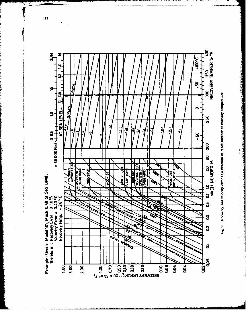
NOW. .-. r r ~ r,~ fr'4

132

CLl

LAn

070

A 0 IIM a

0 L)

0 ID +

00

0 0I

.. .. ....iI. .-

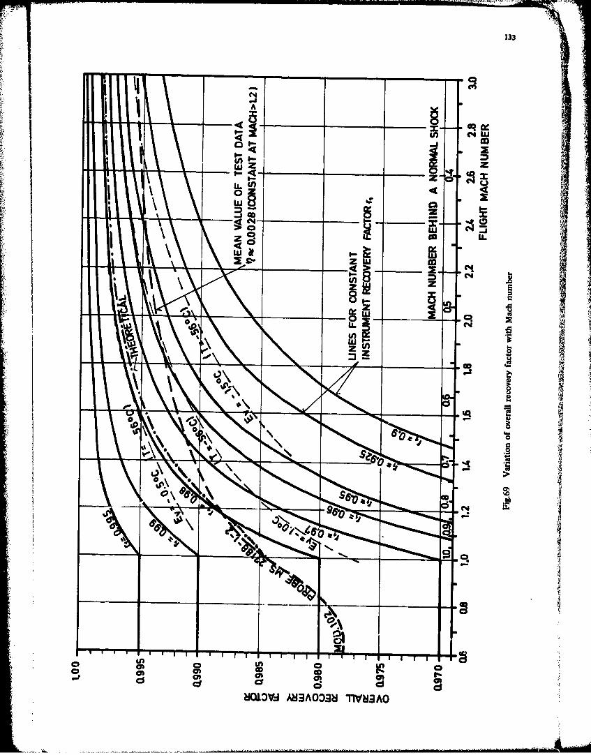
133

1~ U,

090

w I

I-D.

zS e

ILON

C4

_______ _ L\

00c" 0a9

ýJOXDQ AH3AO~33 11VSEAO

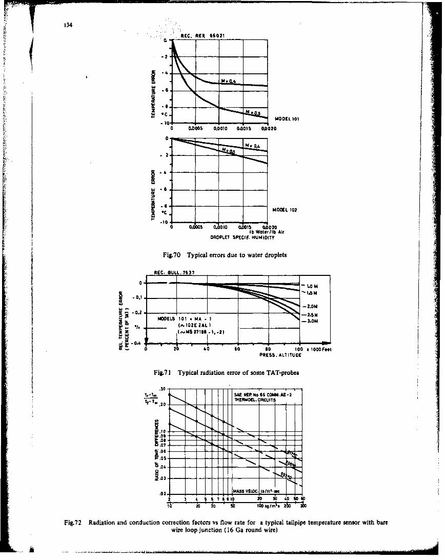
( REC. RER 66021

IO.I

ec MOOEL l0t

0 0.0001 0.0010 0.0015 04020

Xec MOOEL 10

0 =5 010 0 8W5 020 0xOO~~-~~ ~~~~ Water/___ __ P 1bS ALir UD

Fig.7 radicatierons dero tof soter TAT-proets

TREC. BULL 7E637SOMA-

00$

-0.2 -2.-

MODEL -~ it MA MAS 10MC b~t

2 3eM 276611 03 O56

30 60 sokgm~ 10 10 Fo

Fig.2Raiaton ad coducion7 corecionl fadactorisfow errat ofsore aTyiAlTaipproestmeauesn ihbr

wireM Roop jucto (1 Ga round wiE)2

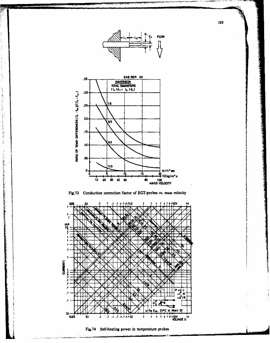
135

d, LOW

s5 SAE REP. 65 ___

IMMERSIONTOTAL DIAMETERS

- .30 ~(I14d4* 111ds1 ____

-30

.20

0*-

iiI 151 - .. .4on. 00 fM.s10 20 30 40 so 90 100

MASS VELOCITY

Fig.73 Conduction correction factor of EGT-probes vs. mass velocity

'It X

0.6 01.mA.4.

4i 7 Sefhetn poe.nte p rtre po e

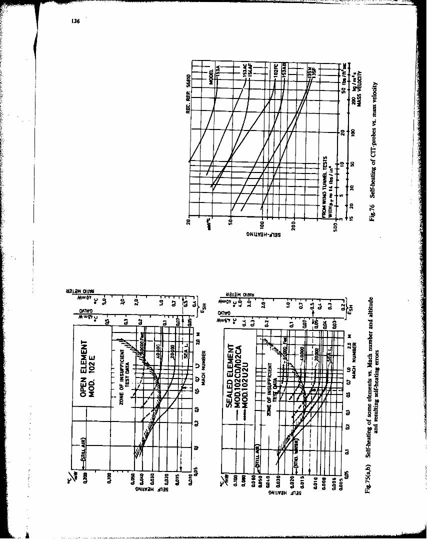
C 0C

~~ I~

MWOT-VT.

; AS

criF d- -0 Id

w -

100w Wd

~$ I 0NNWI a d3f Z=

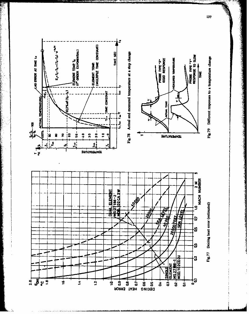
137

00

- IN40U

~ .2

' Tme -- 0o

w- - 00 .,0 0%

000

........... ........ -------- ......------- - - - - - - -------

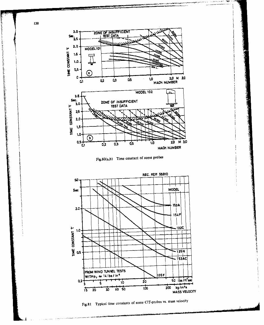
138

3.0 ~ZONE Of IS CE

I- S

i1.O

~0.

0.1 0.2 0.3 to1. 2.0 M 10MACH NUMBER

35 MODEL 102

7 ~ ~ZONE OF INSUFFICIENT ___

?13.0 TEST DATA

0.5 0.O. .5 . . M 3.0MACH NUMBER

Fig.8O(a,b) Time constant of sonmc probes

REC, REP 55880

2-0-

FROM WIND TUNNEL TESTS

WA~ *A1.-/i& 3

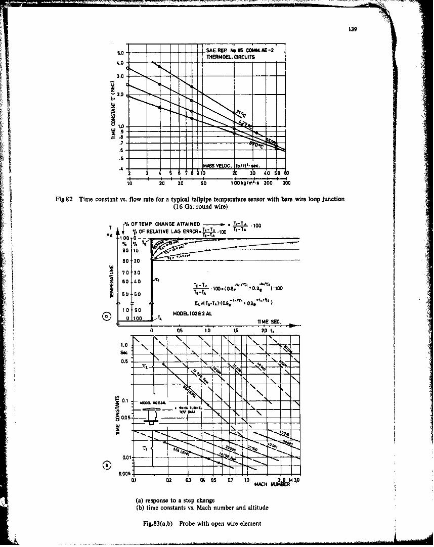
-. .-,--.0139

5.0~~ - - 1 qEREPMOSS CIRCUITS 2

LU

10 20 30 so 1+00 kilm's 200 ý 3400

Fig.82 Time constant vs. flow rate for a typical tailpipe temperature sensor with bare wire loop Junction(16 Ga. round wire)

f/ OF TEMP. CHANGE ATTAINED ----- TE-TA .100

100 OF RELATIVE LAG ERROR.!!..IL.100 Tg-TA--100 .00. T#-TA

1,70 30t

80-27 0 530 T-A ~ *., [

a ia TA MODEL 102E 2ALTIME SEC.

a 0.S 1.0 1.5 2D I,

0.5 21

0.1 MOD.CEL M - -IAa- __________ a INO 1UNNEL _

19SWT DAIA

0.01 -

C 02 0.3 W. Q5 0.7 to 2.0 MAO0MACH NUMBER

(a) response to a step change(b) time constants vs. Mach number and altitude

Fig.83(a,b) Probe with open wire element

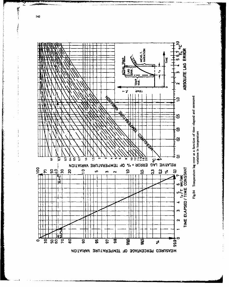
140

i (0

wo

waa

-In

T

x p IN\4

00 00 0 0f -

CO)I~V 0f1~ a~ ~ 0 Ln1~D~ enflV~

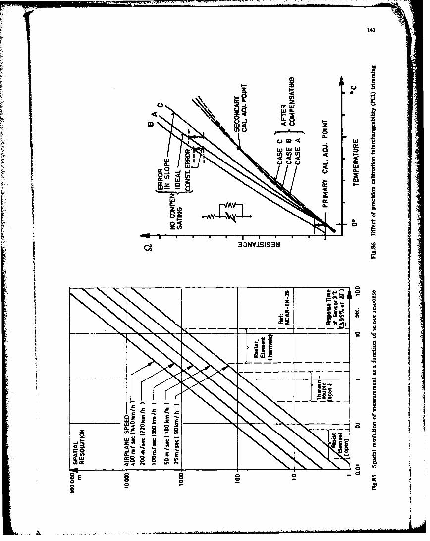
141

cj cr wW C

~MLL4Eau

I-U) U

4c 4 4c

Ix0-jC

CLC

IT I

LU x X

Z.11

c~el- U.2

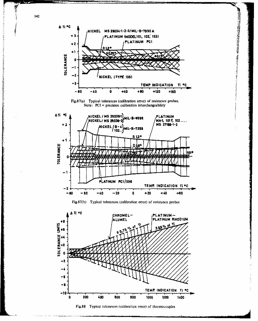
142

N ICKEL MS 2SO34-1-2-3I MIL-B-7990 A

z0-

LuJ -

S-2/NCE YP13)S

-3 TEMP INDICATION TI OC

-60 -0 +44 +90 +420 ,+160

Fig.87(a) Typical tolerances (calibration error) of resistance probes.Note: PCI = precision calibration interchangeability

N~ I NCKEL / MS 250381, M-B-6594 LTIU

t+12

+1

o-

TEMP. INDICATION Ti OC

-80 -60 -40 -20 0 +20 +40 -160

Fig.87(b) Typical tolerances (calibration error) of resistance probes

A Ti 0C

+8 LMLPAIU HDU

zW+w

0-

2.-

TEMP INDICATION Ti OC

0 2,00 40,0 Boo Boo 1ooo i200 , OO0

Fig.88 Typical tolerances (calibration error) of thermocouples

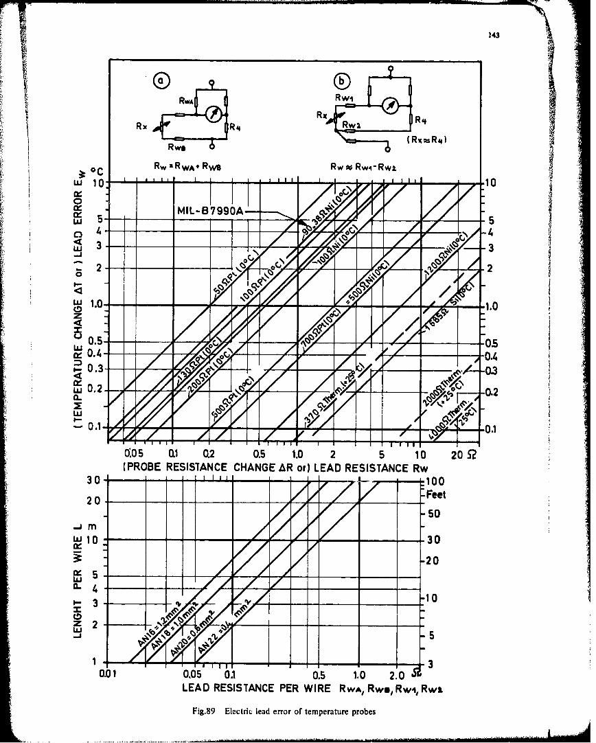
143

Rwi

(RxzsRe)

CRw RWA+ RW Rw w, Rwi Rwi

MIL-B7990A-

w 3 -

z

U _ _

0.5 0 r 0.2

0..1 0.2 0. 1. 5 142

-0300

6.6 01 0.20.5 1.0 2 .5 02(PRO LEA RESISTANCE PHNEAR WIr)EA RESISTANCERwiw

30-.8 Elcr edero1fteprtrepoe

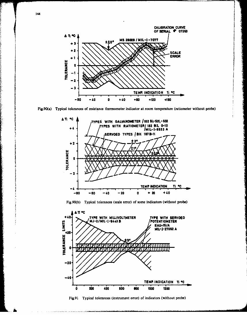
144

CAU1SRATION CURVE

MS 29009 1 MIL-1 -7077

+ IZ.w 0 .

TEMP. INDICATION Ti *C

-60 -40 0 +40 +60 +120 +16'0

Fig.90(a) Typical tolerances of resistance thermometer indicator at room temperature (ratiometer without probe)AT *C TYE IHGLAOMETER /162 BL-501,-502

4 SERVOED TYPES jBH 1675-11

+2

TEMP INDICATION Ti *C

Ki.90b yia oeane saeerr of 0oeidctos(ihu probe)

440 TPWIHMLIOTEETYEWITH SERVOEDMJ-2/MIL I -9'e.3 5 POTENTIOMETER

420

-0

Fig.91 Typical tolerances (instrument error) of indicators (without probe)

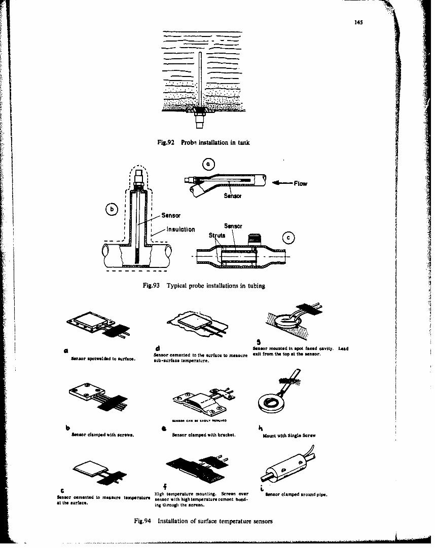
145

Fig.92 ProbW installation in tanik

* 4 - Flow

Sensor

Fig.93 Typical probe installations in tubing

* d Sensor mounted in spot faced cavity. Lead

Sensor cemented to the surface to measure exit from the top at the sensor.

Sensor spotweldad to surface. sub-surface temperature.

b S UNOO CAN U RA6.6 U5MOIAD

Sensor clamped with screws. Sensor clamped with bracket. mount with Single Screw

HeerFi 4 ingh temproturte screntn. Scenoe eorlapdrudpi.Sesrcemented to measure temperature sensor with high temperature cement bond-

Fi.4 Installation of surface temperature sensors

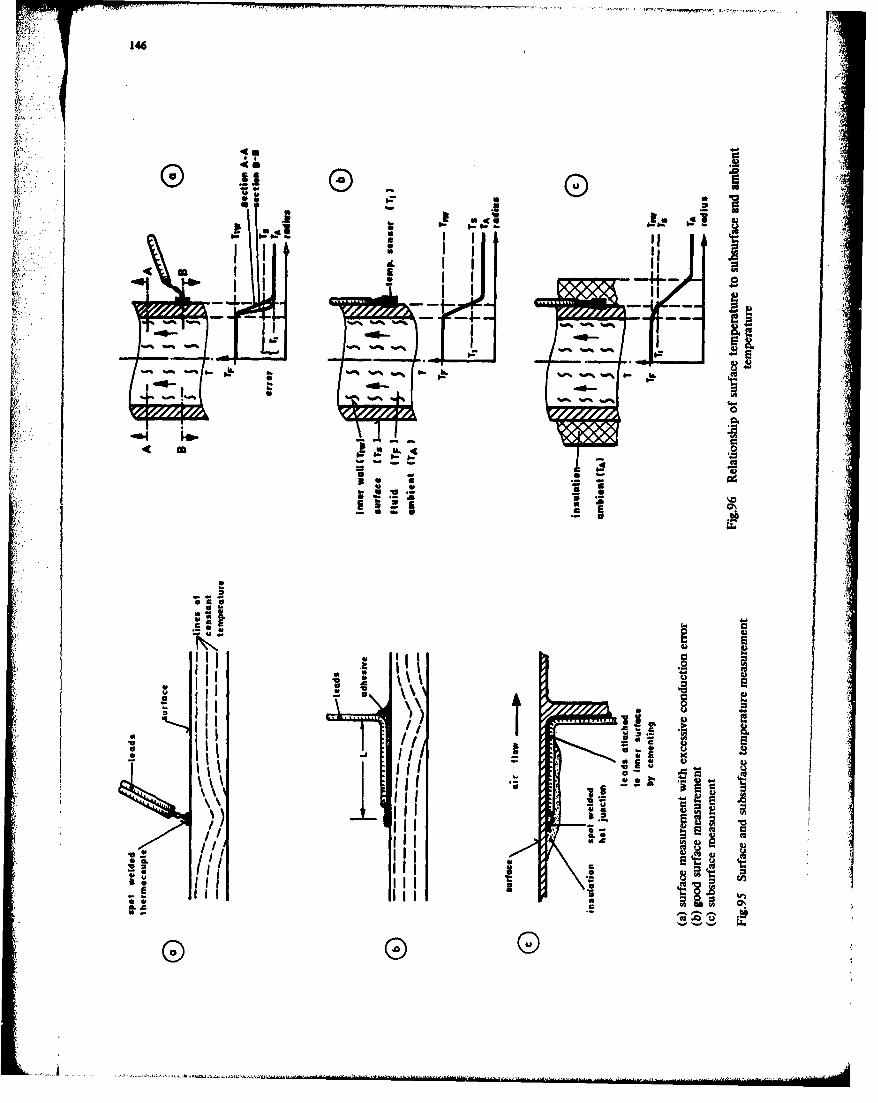
146

S S

__ 4S

(.!) Al

S UU a 0

U .3 w�y. a .3 m�u E.U4U 1 b I- CU

a� b-a-. a I II

4 ii II *1I,

-- 4- --

I �.54- 11�' H-� a.

a - �

a I.= 4)CUa3..

45

- a w

.5'I'

U

Ua -U-

C-

UIII * HIIII a * �

.1 *�5* II, � A �'�.! : \\ A 4)

- I �

U Ii;5- 'II I .

III II £ - � .�

a IaII 3 - S

Hi - 4) 4)1:1 - .5 5,('U I a U5-

IC� iii U� U

'I- 5 5- U � .44U

a -- k

lii .3-

'a.! �'l III a£lie iii a �t�4)

.3 Ii, utI CtIII U 0

30 III III �III IIIbaa- �

o 0 0

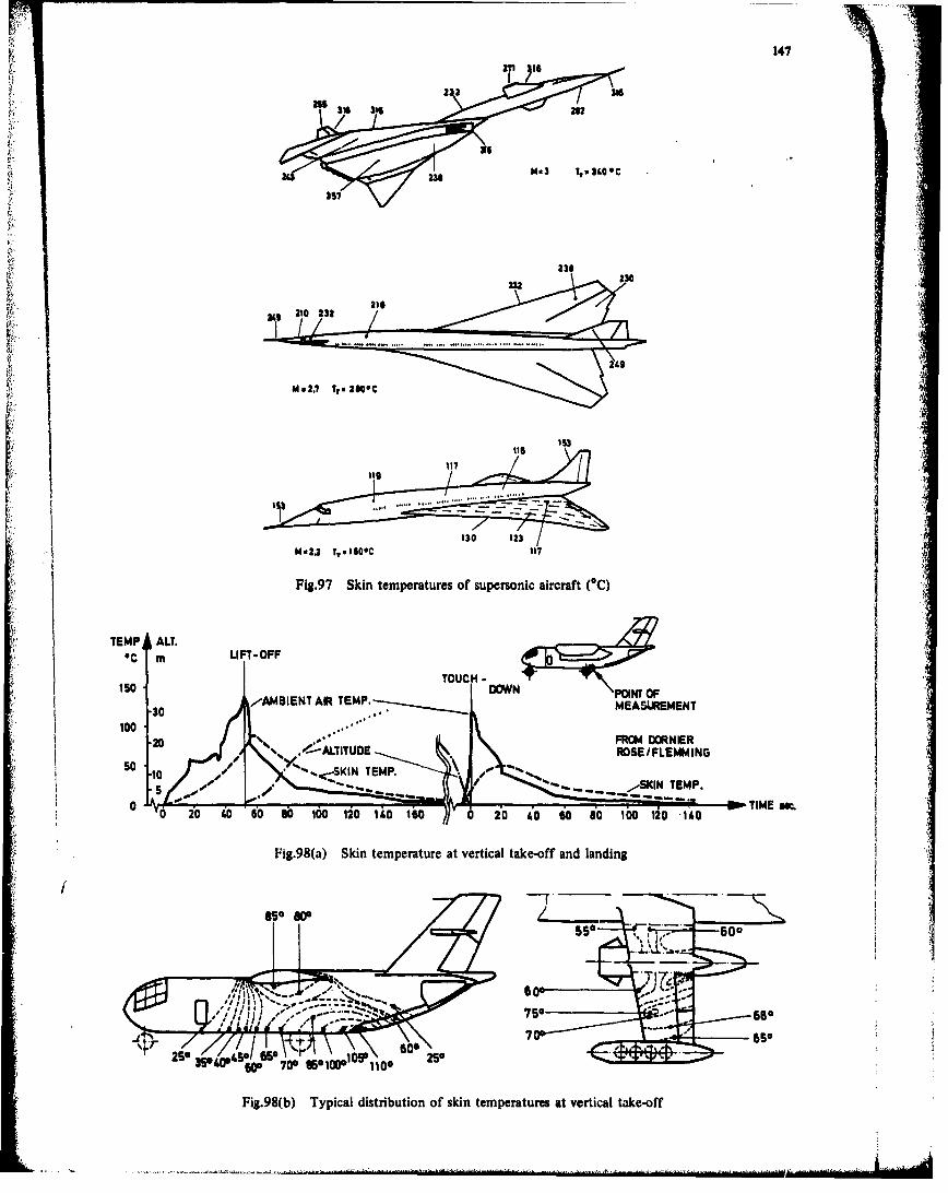
147

411

ISI,10021 2E32EMN

50~ ~ ~~1 10232SI EM.-

... .... .... I TEMP....

0~3 2012M3c

Flg.98(a Skin temperatures at suertical take-offt andla in

550 M,~ LI600 F

100 *O3 10

20.9(b Typica ditiuinoDkntmeaue tvria aeoff

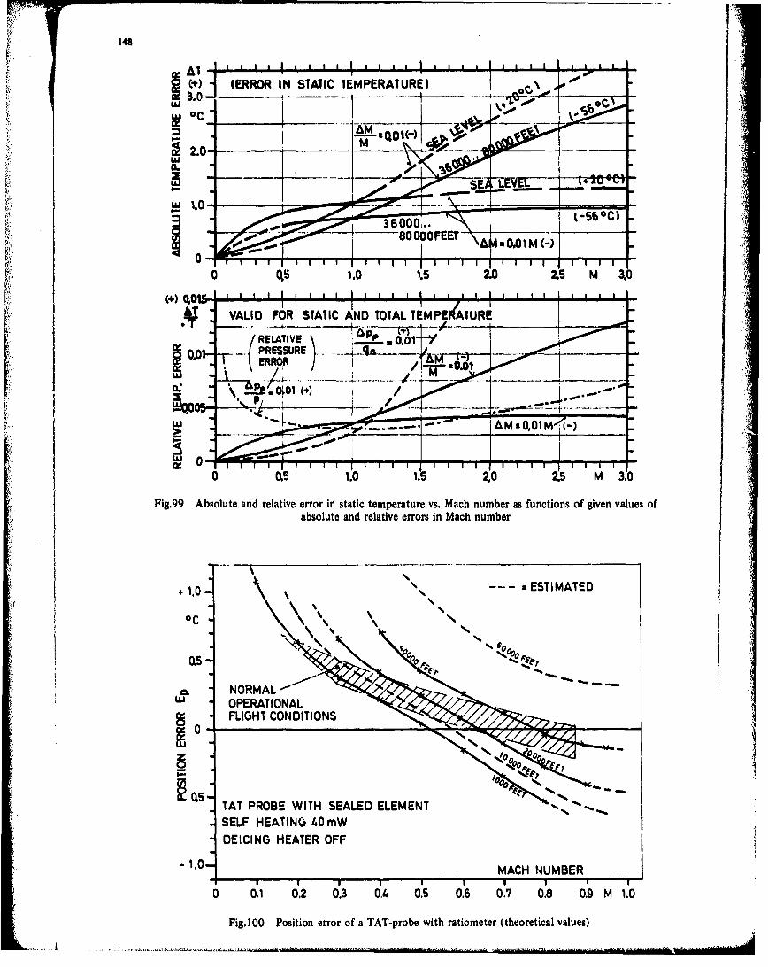
148

() (ERROR IN STATIC TEMPERATURE) 00~3.0

2.0

us10 .1.

000 C ERROR ,t --

'Li 011_ _ _

OPERATIONALo.

TTPROESWTHSELEREEMN

- ~ RO am AC UME

I ý0 I IIo . . . 04 05 06 07 . . .FifO oito ro f A-rb wt aimee tertia aus

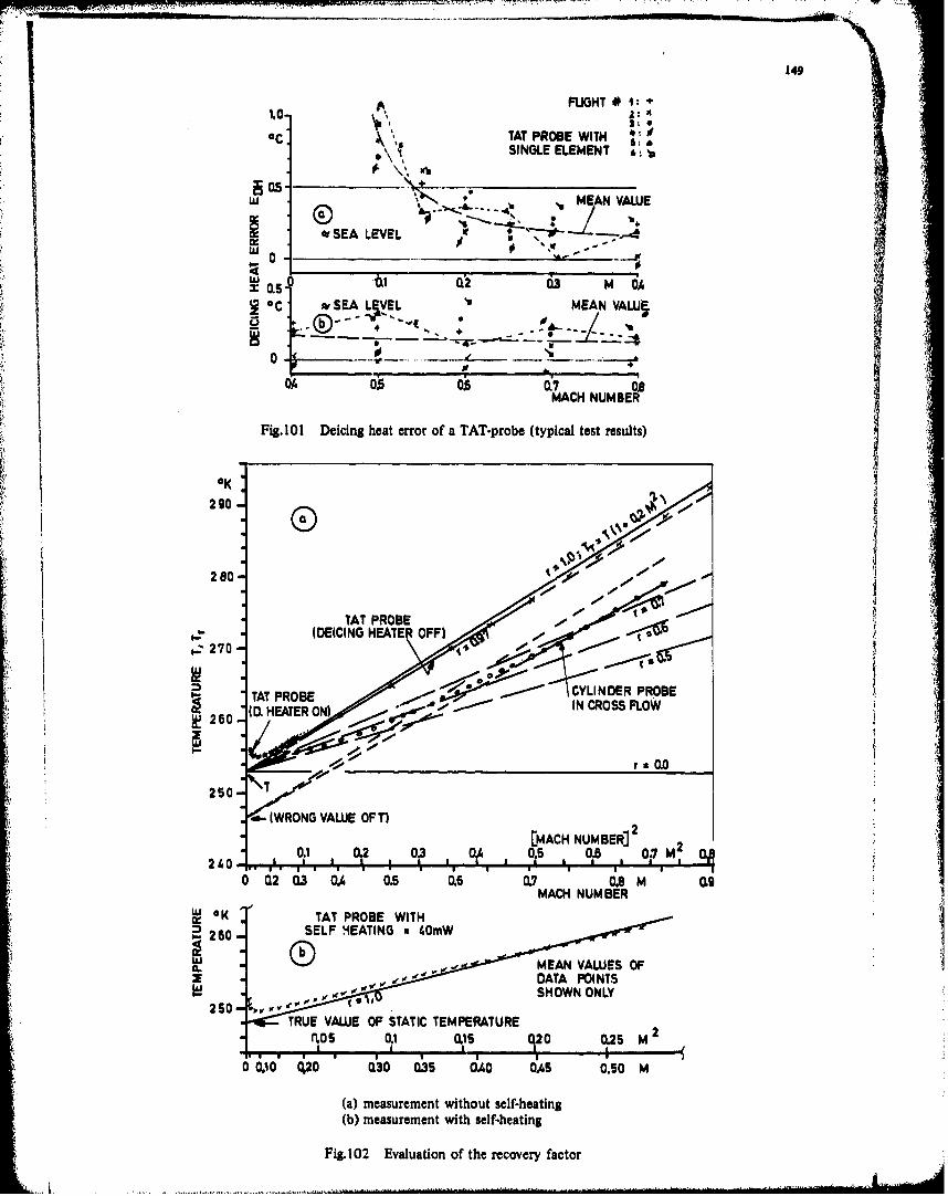
RIM"

149

10 ~FLIGHT 0 1

TAT PROBE WITHSINGLE ELEMENT

05.w "EN "MEAN VALUE

orSEA LEVEL '4

0

CC vSEA, 4VEL MENVAL%~

0A 0ý7 6`70

Fig. 101 Deicing heat error of a TAT-probe (typical test results)

290-~"

280- 10

TAT PROBEOlIDEICING HEATE OFF)

g270-tW~

TAT PROBE A4.CYLINDER PROBE

S20(OLHEATER ON) IN CROSS FLOW

r 20.0

00.20.3 ~ o~ [MACH NUMBER] 2

0jSOh203 Q 0.5 0.6 0.7 0*b M

aw O TAT PROBE WITHMAHN BEN-260- SELF 4EATING 4 OmW

0'060 0.20 Q30 035 OhO OAS 0.50 M

(a) measurement without self-heating

(b) measurement with self-heating

Fig. 102 Evaluation of the recovery factor

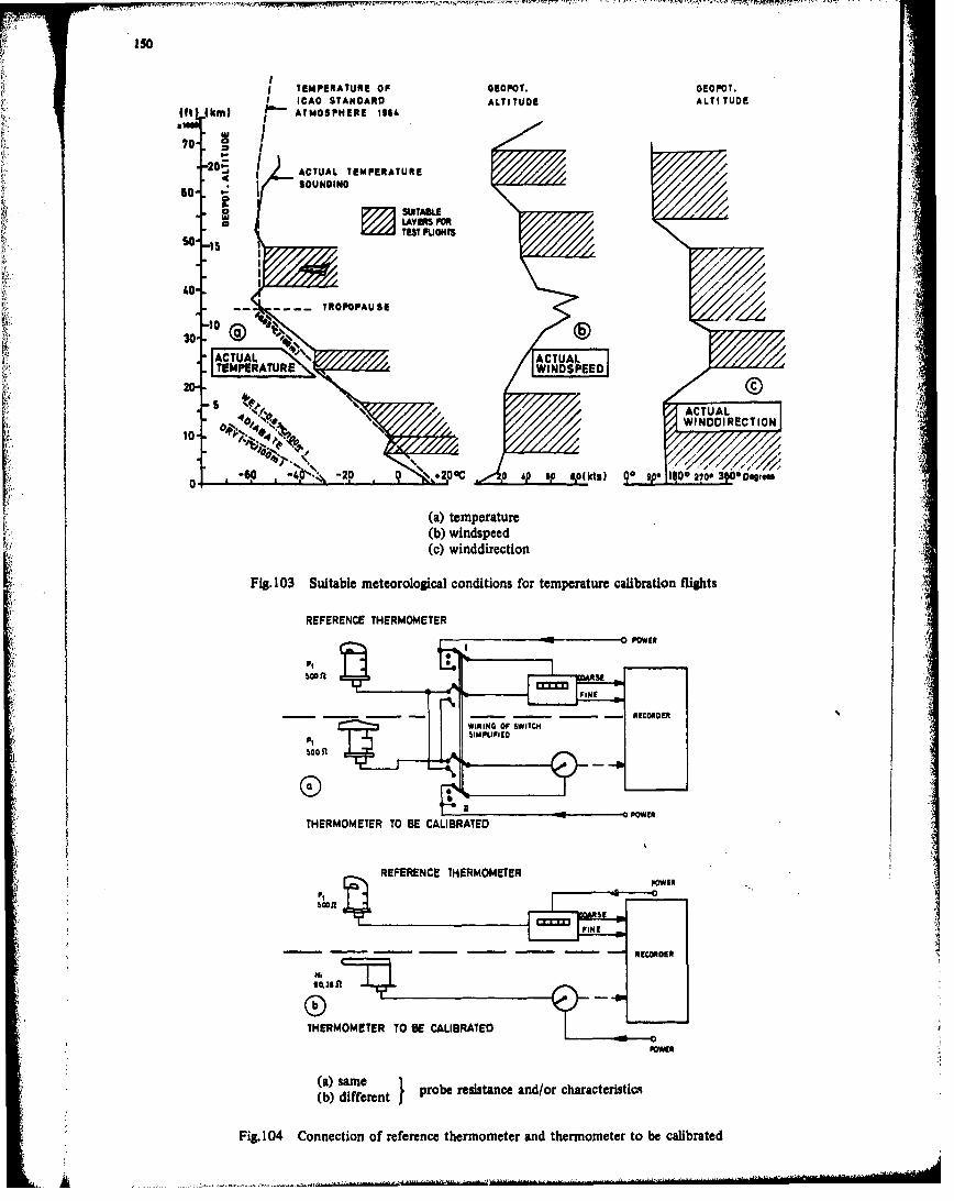
I TEMPERATURE OF GEOPOT. EOPOT.

If (m ICAO STANDARD ALTITUDE ALTI TUDE

70-. I~ g ACTUAL TEMPERATURE

I SOUNDINO,

a I7~SUIT~k

40.

10®%) TROPOPAUSE

30

FiA F'N%. ACTUALTEMPEATUREWINOSPEED

-S ACTUALWINDDIRECT ION

(a) temperature(b) windspeed(c) winddirection

Fig. 103 Suitable meteorological conditions for temperature calibration flights

REFERENCE THERMOMETER

No 0 POWER

S01 1

WIRIN orSII

THERMOMETER TO BE CALIBRATED

REFERENCE THERMOMETER

Pt

- - - RECORDERt

THERMOMETER TO BE CALIBRATED O

(a) same 1probe resistance and/or characteristics(b) different

Fig. 104 Connection of reference thermometer and thermometer to be calibrated

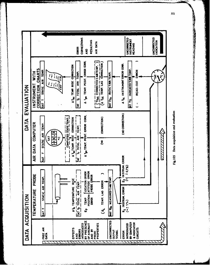
-0 0 I I..t. L ~ ~

U) I-

W0

z~ Z04..a

1,1 - 0

-. z

o U Z-w Z t ' i

8 a8 8

Li UU,

w A: n:

0a U ~I4 ;5 co

C- w

5 w~ a-

o in Z_ L__ _ ___ _

0 ILZ z 15.

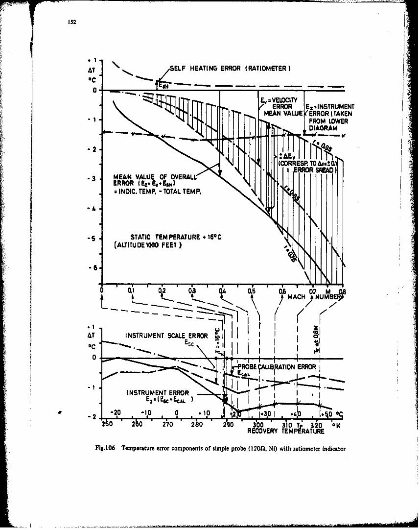
152

AT SELF HEATING ERROR (RATIOMETER)

IT~rr. EyVELOCITY-. '"4.1'i41111 ERROR VLEsEsINSTRUMENT(TKNRO

-1FROM LOWERDIAGRAM

.2.AEv 11

-3 MEAN VALUE OF OVERALLERROR IEZ*EV.Esm) 1

aINDIC. TEMP. -TOTAL TEMP.

-6 STATIC TEMPERATURE *160C(ALTITUDEIOOO FEET)

SMACH)'NUMS?

AT INSTRUMENT SCALE ERROR c I I I0C

ROBECA EALIBA ION ERROR

-20 -10 0 +.100

20 2h0 200 280 20 300 310 T 320 OKRECOVERY TEMPIRATURE

Fig. 106 Temperature error components of simple probe (1 2012, NI) with ratiomneter indicator

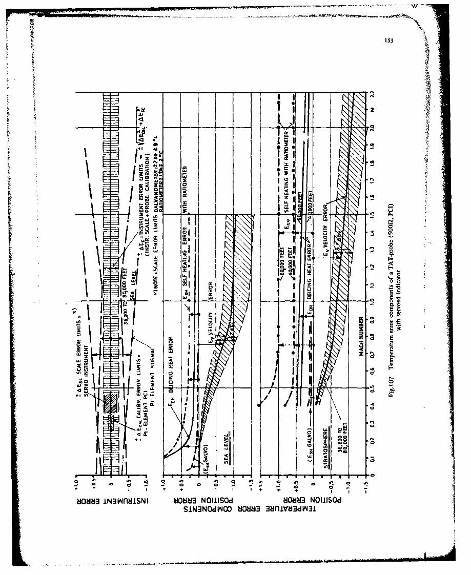
wt

IS3.

fuj

Z 4

NAN

LI

0 i

cc 0* 0

",i qg

00 .

't I 'a. I M ILa z

0 W

-J a:

2-

+ + +

NI iNpnwN H08 N+I~ 808 N I I I

SiN3NOdINOO 80883 UnMUV~~dIN

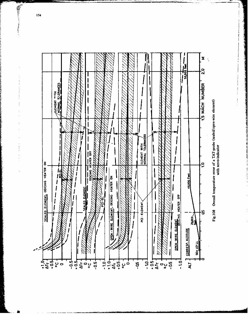
154

*f

z IIJ

- x

I 4'K '4 -.

00

I"

uj 06

-I-' VZ__ LU LUZ

a

1Ii1 \\I

-j 00

I -a Lo

z $4

I ~ _

1A ' /4 dr-4

I c; C3Cp3-I I >1t I~i Cn+r 0~ + 0 0

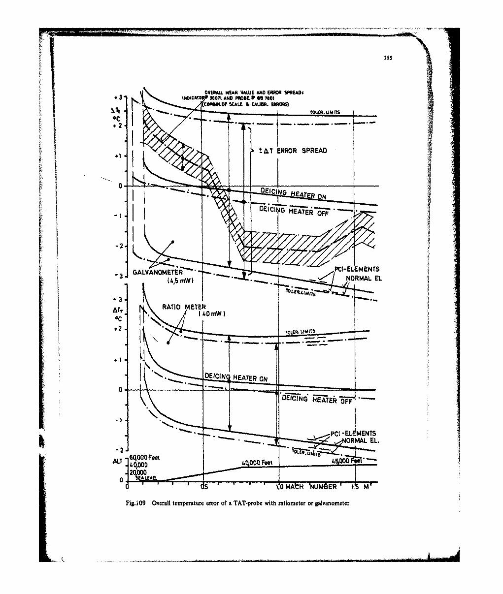
OVER"L 14FAN VALUE ANDO ERWRO SPREADs.3 1"MocA 30071 AND PROBE4 0 6 730)COMM NOf SCALE 3CAUBSR. IEOI0 4

oc -.2

0

AA

GALVANOMETEIZ ,PC(-ELEMENTS

.3

RATIO METER

DEDEUCIG HEATER OON

-2 PCI ELEMENTS

AT6C4O00 Feet

Fig. 109 Overall temperature error of a TAT-probe with ratiometer 0r galvanometer

.~. ............... .......

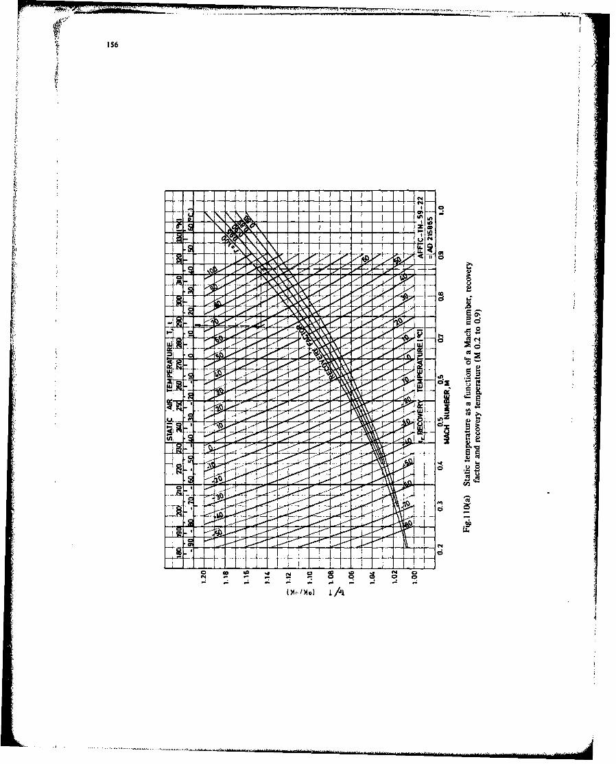
156

at

-~ -4 -~ ILI IN - - to

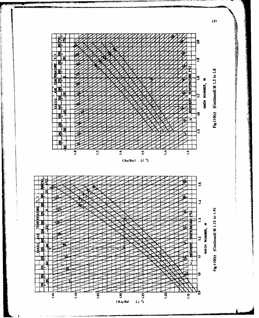
157

ow-

-. 00

-L - - - - <

CC44

.P- .4

* Acz

()0)0 1 .- i

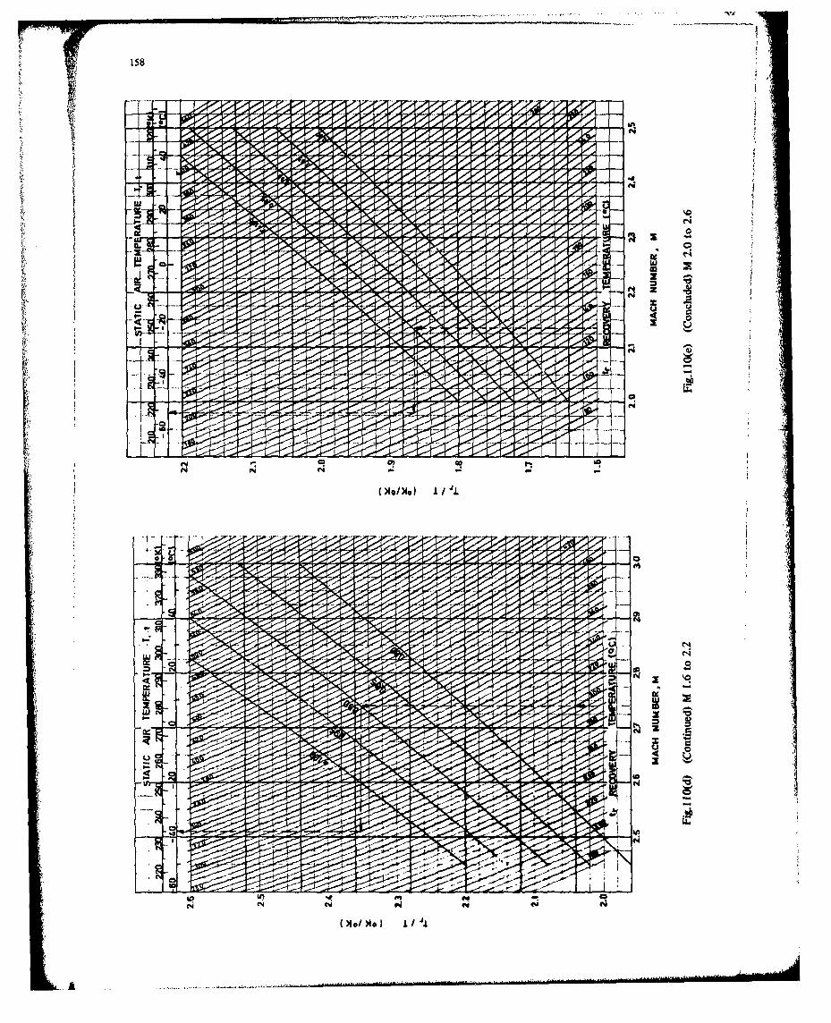
158

000

Ap ...

Xe/ )1) 1 J

N NN

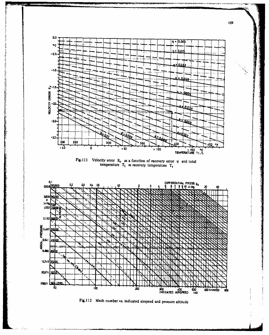
~.J-~7 -. 30

-NIAE A kR-E A

Fig. 11 Ma Vlcht nmerrr vas. i fndcated n airs e oed y adpesreo 1 altitude l

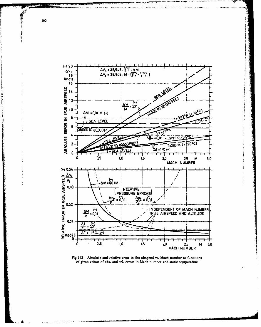
160

()20 II I I I ' I -

AVj z38,94S.fl .. &M1not 4Vt z38.94.5- MiT-VT r)

Knt - I

J16

1'~ ~ ~ ~ L 3600108,00F _4,

0C. . 15202, .MAC NUMBE

1VV +/4Uj Vto

L'a 0.01 M

u .~ .0 0 3 _ _ _ _ _ _ _ _ _ _ _ _ _ _ _ _ _ _ _ _ _ _ _ _ _ _ _ _ _ _ _ _ _ _ _

0 .z. . . . .-7ý-SMACH NUMBER- 6 _4

Fig 1 13 bolt a nd0 reaieerri hearpe s ah ubra ucinofgvnvlewfas n e.err nMc ubradsai eprtr

UAK -