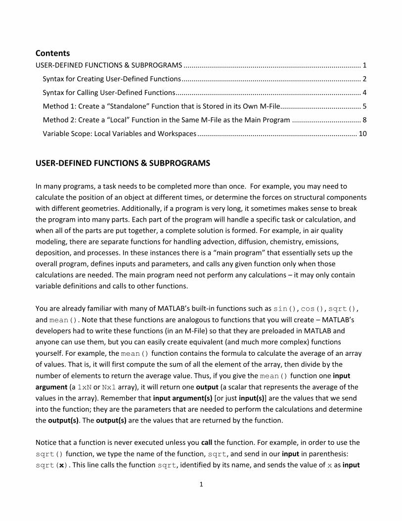
1

Contents

USER-DEFINED FUNCTIONS & SUBPROGRAMS .......................................................................................... 1

Syntax for Creating User-Defined Functions ........................................................................................... 2

Syntax for Calling User-Defined Functions .............................................................................................. 4

Method 1: Create a “Standalone” Function that is Stored in its Own M-File......................................... 5

Method 2: Create a “Local” Function in the Same M-File as the Main Program ................................... 8

Variable Scope: Local Variables and Workspaces ................................................................................. 10

USER-DEFINED FUNCTIONS & SUBPROGRAMS

In many programs, a task needs to be completed more than once. For example, you may need to

calculate the position of an object at different times, or determine the forces on structural components

with different geometries. Additionally, if a program is very long, it sometimes makes sense to break

the program into many parts. Each part of the program will handle a specific task or calculation, and

when all of the parts are put together, a complete solution is formed. For example, in air quality

modeling, there are separate functions for handling advection, diffusion, chemistry, emissions,

deposition, and processes. In these instances there is a “main program” that essentially sets up the

overall program, defines inputs and parameters, and calls any given function only when those

calculations are needed. The main program need not perform any calculations – it may only contain

variable definitions and calls to other functions.

You are already familiar with many of MATLAB’s built-in functions such as sin(), cos(), sqrt(),

and mean(). Note that these functions are analogous to functions that you will create – MATLAB’s

developers had to write these functions (in an M-File) so that they are preloaded in MATLAB and

anyone can use them, but you can easily create equivalent (and much more complex) functions

yourself. For example, the mean() function contains the formula to calculate the average of an array

of values. That is, it will first compute the sum of all the element of the array, then divide by the

number of elements to return the average value. Thus, if you give the mean() function one input

argument (a 1xN or Nx1 array), it will return one output (a scalar that represents the average of the

values in the array). Remember that input argument(s) [or just input(s)] are the values that we send

into the function; they are the parameters that are needed to perform the calculations and determine

the output(s). The output(s) are the values that are returned by the function.

Notice that a function is never executed unless you call the function. For example, in order to use the

sqrt() function, we type the name of the function, sqrt, and send in our input in parenthesis:

sqrt(x). This line calls the function sqrt, identified by its name, and sends the value of x as input

2

to the function. The function will then return the output, which will be the square root of x. Notice

that when we call a function, we need to have a variable to the left-hand side of the equals sign to

store the output of the function (otherwise it will be stored to the default ans variable, which is

undesirable). Thus, the line of code that calls the function sqrt, sends the value of x as input, and

saves the output to a variable called sq_x would look like the following:

sq_x = sqrt(x)

When a function has more than one output, you need to provide more than one variable to the left of

the equals sign to store the values of all the outputs. You have most likely already experienced this

when using the built-in size() function. This will be discussed in more detail later when we cover

examples of user-defined functions with multiple outputs.

Note that functions may only accept certain types of input arguments and/or return certain types of

outputs, and that the type of output returned may depend on the input. For example, the sqrt()

function will accept scalars or numerical arrays as input, but not character arrays. Additionally, the

output will depend on the input. If went send a scalar x as input, the output will be a scalar that

represents the square root of x. However, if we send an array x as input, the output will be an array of

the same dimensions as x, where each element of the output array is the square root of the

corresponding element of in input array. Notice too that different functions behave differently; if we

send a MxN array as input to the mean() function, the output will be a 1xN array of values (this

function takes the mean of each column of values). Thus, we need to be mindful of the inputs and

outputs when we are creating and calling our own user-defined functions.

Syntax for Creating User-Defined Functions

Now that you know some basic terminology and see how built-in functions operate, let’s see how we

can write our own functions to perform any tasks/calculations that our program needs to do. First, let’s

look at the syntax used to create a user-defined function:

function [outputs, listed, here] = function_name(inputs,listed,here)

% Comments that describe the function and its use/purpose

% - These show when you type “help function_name”

<Commands / Statements / Calculations go here>

<Use anything you have learned in MAE10>

end

When creating a function, we always start with the keyword function.

3

After that, on the same line, we list any outputs. The outputs will be variables that we define

(assign values to) inside the function. The outputs will hold the results of the calculations that

we perform inside the function so that they can be passed back to the main program (or

another function) that called the function_name function.

o A function can have any number of outputs, including none.

If a function has no outputs, you can omit the square brackets (and the equals

sign as mentioned below).

o If the function has more than one output, the output variables must be enclosed in

square brackets (analogous to how the disp() command requires square brackets

when it has more than one argument).

The square brackets are not required if the function has zero or only one output.

After listing the outputs, you put a single equals sign, then the name of the function

(function_name in the above example). The same rules for valid variable names apply to

function names.

o If the function does not have any outputs, you can omit the square brackets and equals

sign as mentioned above. In this case, you simply put the word function, followed by

the name of the function.

After the name of the function, you list any input arguments enclosed in parenthesis and

separated by commas. The inputs are values that are passed into the function when it is called;

they are the values that we need inside the function to perform the calculations that determine

the values of the outputs.

o A function can have any number of inputs, include none.

o If a function has no inputs, you can omit the parenthesis altogether, meaning that the

function definition line will stop after the name of the function.

The first few lines inside the function are typically used to provide some documentation on the

function in the form of comments. These comments can describe what the function does, what

inputs are needed, what the outputs are, warnings to the potential user, and so on.

o Including comments in the beginning of your function allows you to use the help

command to get information about the function (just as you would for getting quick

help on a built-in function in the command window). Any comments that are included as

the first few lines inside the function will show up when you type “help

function_name” in the command window. This only applies to standalone functions

and not local functions (discussed below).

Inside the function we can use anything we have already learned in MAE10: if statements,

loops, fprintf(), etc. Any commands that you can use in a regular script M-File you can use

inside a function.

4

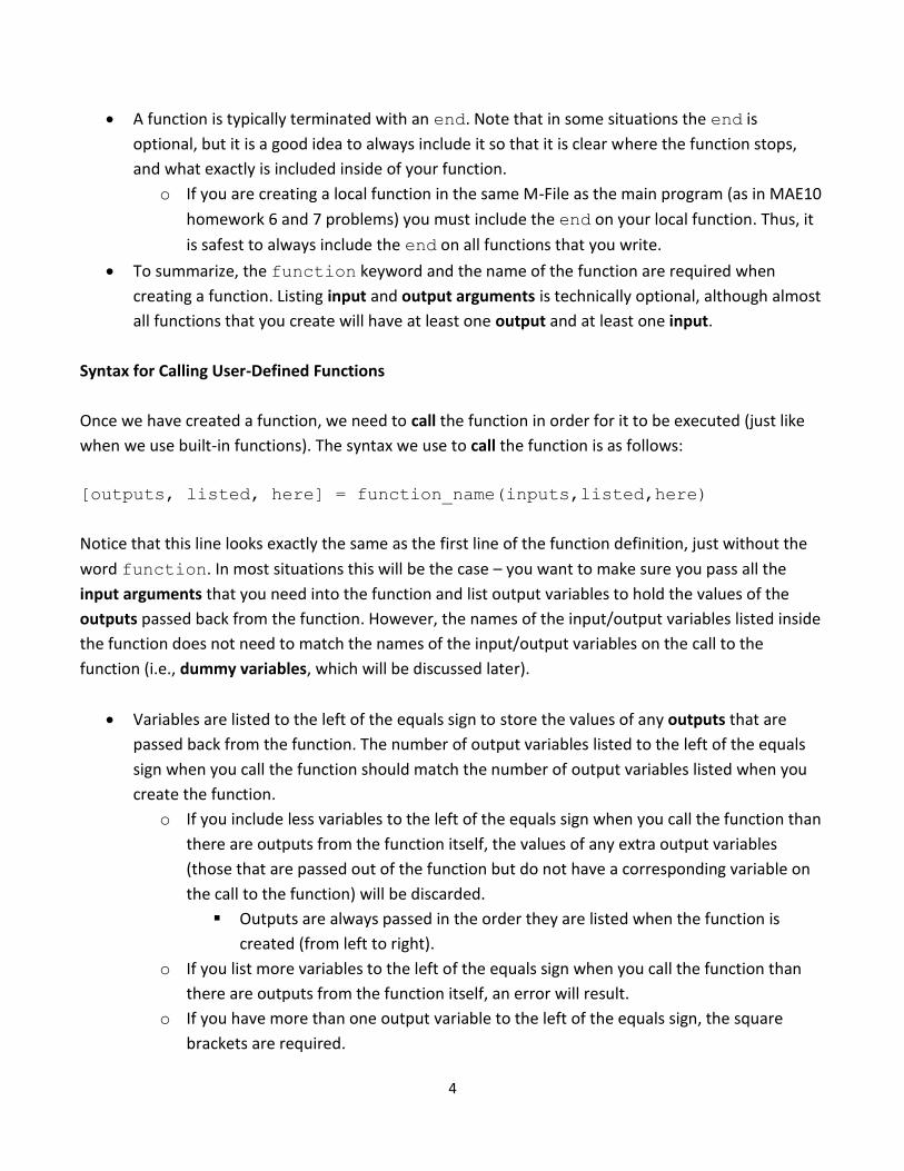
A function is typically terminated with an end. Note that in some situations the end is

optional, but it is a good idea to always include it so that it is clear where the function stops,

and what exactly is included inside of your function.

o If you are creating a local function in the same M-File as the main program (as in MAE10

homework 6 and 7 problems) you must include the end on your local function. Thus, it

is safest to always include the end on all functions that you write.

To summarize, the function keyword and the name of the function are required when

creating a function. Listing input and output arguments is technically optional, although almost

all functions that you create will have at least one output and at least one input.

Syntax for Calling User-Defined Functions

Once we have created a function, we need to call the function in order for it to be executed (just like

when we use built-in functions). The syntax we use to call the function is as follows:

[outputs, listed, here] = function_name(inputs,listed,here)

Notice that this line looks exactly the same as the first line of the function definition, just without the

word function. In most situations this will be the case – you want to make sure you pass all the

input arguments that you need into the function and list output variables to hold the values of the

outputs passed back from the function. However, the names of the input/output variables listed inside

the function does not need to match the names of the input/output variables on the call to the

function (i.e., dummy variables, which will be discussed later).

Variables are listed to the left of the equals sign to store the values of any outputs that are

passed back from the function. The number of output variables listed to the left of the equals

sign when you call the function should match the number of output variables listed when you

create the function.

o If you include less variables to the left of the equals sign when you call the function than

there are outputs from the function itself, the values of any extra output variables

(those that are passed out of the function but do not have a corresponding variable on

the call to the function) will be discarded.

Outputs are always passed in the order they are listed when the function is

created (from left to right).

o If you list more variables to the left of the equals sign when you call the function than

there are outputs from the function itself, an error will result.

o If you have more than one output variable to the left of the equals sign, the square

brackets are required.

5

o If you have only one output variable, the brackets enclosing the output variable list are

not required (but can still be included, similar to using the disp() command).

o If you have no outputs, you can omit the list of output variables and the equals sign, and

the call to the function will begin with the name of the function.

The list of output variables (if any) is followed by an equals sign, and then the name of the

function. When calling a function, be sure to use the full function name exactly as it appears

when you define the function.

Immediately following the name of the function, any input arguments are listed in parenthesis

and separated by commas.

o The number of input arguments listed when calling the function must be exactly the

same as the number of inputs listed when the function is defined if all the inputs are

used inside the function to perform calculations. Including too few or too many input

arguments when trying to call a function will produce an error.

There are two different ways that you can create user-defined functions in MATLAB that we will learn

in MAE10. While the content and syntax of the function definition is exactly the same in both methods,

there are important differences between the two methods in the way the files that contain the

functions are structured and the way the functions are accessed. These two methods are discussed in

detail in the following sections.

NOTE: Anonymous functions, a special type of function in MATLAB, are discussed in a separate

document.

Method 1: Create a “Standalone” Function that is Stored in its Own M-File

The first method for creating functions that we use in MAE10 is to write the function in its own M-File.

The first line of this M-File should be the function definition line. That is, the line that contains the

word function, the list of outputs (if any), the equals sign, the function name, and the list of inputs

(if any). The limitation of the standalone method is that the function must be in its own M-File,

separate from the main program or script that calls it, and the name of the M-File must match the

name of the function. The reason is that MATLAB will only be able to find this function by locating an

M-File with the same name. When you use this method, you are essentially creating a new built-in

function – you can call this function from the command line or from any other M-File so long as the M-

File that contains the function is in your current working directory (Current Folder in MATLAB). Let’s

look at an example of a standalone function to illustrate this method.

6

In my_func.m:

function [out1,out2,out3] = my_func(a,b,c)

% Include comments that describe my_func here

out1 = a + b + c

out2 = a * b * c

out3 = 10

end

In the command window:

>> [x,y,z] = my_func(7,5,2)

out1 =

14

out2 =

70

out3 =

10

x =

14

y =

70

z =

10

In my_func.m we define the function called my_func that has three inputs and three outputs. This

time we are passing values directly into the function when we call it (7, 5, 2), but we could also list

variables here if they have values stored in memory. Inside the function there are some basic

calculations to determine the values of the output variables, which are then passed back to where the

function is called, which in this case is the command window. Notice that the names of the output

variables listed inside my_func.m where we define the function did not match the names of the

7

variables in the command window when we call the function. Again, this is not a problem for MATLAB,

and the important thing to remember is that the values of the inputs and outputs (regardless of the

variable names) are passed from the function file to the command window, in the order they are listed,

which you can see from what is displayed in the command window during execution. Notice that the

variables out1, out2, and out3 are calculated and assigned values first since they are inside the

function. Then, after the function finishes, it passes the values of these three variables to the three

variables listed to the left of the equals sign when the function is called, in the order they are listed.

Thus, since x is the first output variable listed on the function call, it takes the value of the first output,

out1, and so on for y and z.

The next thing you might notice is that there are a lot of variables displayed in the command window

during execution. We get variables’ values displayed in the command window from inside the function

when we calculate the values of the outputs since they are not suppressed, and we also get values

displayed from when the function call is finished and x, y, and z are assigned values in the workspace.

We can also call this function from another M-File (in the same folder on your computer). In this

example, we will define our inputs as variables rather than passing values directly, and call the function

from a separate M-File than the one that contains the function.

In my_func.m:

function [out1,out2,out3] = my_func(a,b,c)

% Include comments that describe my_func here

out1 = a + b + c

out2 = a * b * c

out3 = 10

end

In my_file.m:

a = 5;

b = 1;

c = 9;

[red,blue,green] = my_func(c,b,a)

In the command window:

>> my_file

out1 =

15

8

out2 =

45

out3 =

10

red =

15

blue =

45

green =

10

Notice that we execute the M-File my_file.m that contains the main program – we do not execute

the function file. When we execute my_file.m, it defines the values of a, b, and c, calls the function

my_func, and passes in the values of the input variables. Inside my_func.m it follows the same

procedure described above, where it first calculates the values of the outputs and then when the

function is finished, it passes the values of the outputs back to where the function is called, which in

this case is my_file.m, rather than the command window. We again use different variable names for

the output variables in my_file.m than the output variables in my_func.m to illustrate that the

names of the variables is not important, the order and values of the variables is key.

Method 2: Create a “Local” Function in the Same M-File as the Main Program

The other method for creating user-defined functions in MATLAB is to write the function in the same

M-File as the main program. This is called a local function, because it is in the same M-File as the main

program and it can only be called and used from within this M-File. This means that we cannot call

local functions from the command line or from any other M-Files.

In this construct the main program must come first in the M-File, then one or more local functions can

be defined after (below) the main program. This is the method that is required for MAE10 homework

problems because it allows us to choose any filename for the M-File that contains both the main

9

program (given) and the function (that you must write to solve the problem). Thus, be sure to stick to

the file naming convention when creating and uploading your homework M-Files to the EEE DropBox.

The main program typically just defines parameters and variables that will be passed as input to the

local function to perform the calculations. The main program itself need not perform any calculations.

You will see this in homework 6 and homework 7 problems where you are given the main program but

must create the local function that performs the calculations necessary to solve the problem. The

inputs variables are defined in the main program and passed to the local function when it is called, and

the function calculates the values of the outputs and passes them back to the main program. In the

following example, we will use exactly the same function, my_func, as in the previous example. The

only difference will be how we construct the M-File, which in this case will contain both the main

program and the local function my_func.

In any_file_name.m:

% Put main program first (at top of M-File)

a = 5;

b = 1;

c = 9;

[red,blue,green] = my_func(c,b,a)

% Define one or more local functions after main program

function [out1,out2,out3] = my_func(a,b,c)

out1 = a + b + c

out2 = a * b * c

out3 = 10

end

In the command window:

>> any_file_name

out1 =

15

out2 =

45

out3 =

10

10

red =

15

blue =

45

green =

10

In this example we have essentially merged the two M-Files from the standalone function example

together into one M-File that contains both the main program and the function. Notice that the main

program and the function contain exactly the same code in both examples. We essentially just moved

the main program from my_file.m to the top of any_file_name.m and moved the function from

my_func.m to any_file_name.m (below the main program).

However, since the M-File now contains both the main program and the function my_func,

my_func is now a local function. This means that we cannot call my_func from the command line or

from any other M-File; it can only be accessed and used from within the same M-File that it is defined.

The benefit is that we can now name the M-File anything we like, and the function is now contained

within the same M-File as the main program so we don’t have to worry about making sure the function

M-File is in the same directory as the main program M-File.

Variable Scope: Local Variables and Workspaces

Before learning about user-defined functions, any variable that you declared (assigned a value to) from

the command line or within an M-File was automatically saved in the workspace. You could see this

variable in MATLAB’s GUI or list all variables currently in the workspace using commands like who or

whos. More specifically, this is called the base workspace. Variables stored in the base workspace

remain in memory until you clear them or exit MATLAB. However, functions do not use or access the

base workspace. Every function uses its own, completely separate, function workspace. Each function

workspace is different from the base workspace and all other function workspaces. Even local functions

in the same M-File each have their own separate workspaces. Therefore, variables that are defined

(assigned a value) inside the main program or from the command line are not automatically defined

within a function. For this reason, any variable’s value that we need inside a function must be passed in

as an input.

11

Similarly, variables that are defined (assigned a value) inside a function are not automatically defined

in the base workspace that you see in MATLAB’s GUI. Each function stores variables locally, meaning

that they are only defined within that specific function. In other words, each function has their own

function workspace, which is completely separate from the base workspace shown in your MATLAB

GUI. Variables defined inside functions will not show up in the base workspace that you can see, nor

will they show up when using commands that access the base workspace like who or whos. Thus, if

you need a variable’s value that was calculated inside a function to be available in the main program

(base workspace), you must pass this value out of the function as an output.

NOTE: Technically, it is possible to never use functions in your MATLAB codes. However, your codes

may become unnecessarily complicated and lengthy if you do not use them. Additionally, using

functions allows you to easily track down errors and debug your code since specific calculations are

isolated to certain functions.

Let’s summarize user-defined functions by comparing and contrasting the similarities and differences

between standalone and local functions:

Standalone Functions

o Use this method when you want to create a more generally applicable function that can

be called from the command line or will be used by many different programs that you

write.

o Standalone functions must be placed in their own M-File and the name of the function

must match the name of the M-File. There should be no main program or any other

code in the M-File that contains the standalone function.

o To call/use a standalone function, it must be in the same directory (e.g., in your Current

Folder) as the M-File that calls it. MATLAB locates the function by looking for a filename

with the same name as the function, and it only searching in your Current Folder.

Local Functions

o Use this method when you are creating a more specific and specialized function that will

be used only by the program that is located in the same M-File as the function.

o Local functions must be placed after (below) the main program in the M-File.

o Since the local function is located in the same M-File as the main program, you do not

need to worry about any other M-Files when running the program. MATLAB will

automatically scan the M-File for the function (by its name) when it is called.

The syntax for creating and calling the functions is the same in both cases. Although it is

technically optional in certain situations, it is good practice to always include an end to signify

the end of your functions.

12

Remember that the names of the input/output variables listed when the function is called do

not need to match the names of the variables listed when the function is defined. The values

are passed in the order the variables are listed.

Remember that variables declared in the main program (which uses the base workspace) are

not automatically defined inside of a function (which uses a completely separate function

workspace). Any variable’s values that you need to send into the function or pass out of the

function must be transferred via the functions inputs and outputs. This applies to both local and

standalone functions.

o In other words, the only way that functions exchange values with the main program or

other functions is through the function’s inputs and outputs.