Aft Notes 12

7/30/2019 Aft Notes 12

http://slidepdf.com/reader/full/aft-notes-12 1/80

Advanced Quantum Field Theory

Dr Arttu Rajantie2011/12 Second Term

Contents

I Path Integral Quantization 3

1 Derivation of the Path Integral 3

1.1 Heuristic Argument . . . . . . . . . . . . . . . . . . . . . . . . . . . . . . . . . . . . . . 3

1.2 Quantum Mechanics . . . . . . . . . . . . . . . . . . . . . . . . . . . . . . . . . . . . . 41.3 Many Particles . . . . . . . . . . . . . . . . . . . . . . . . . . . . . . . . . . . . . . . . 6

1.4 Scalar Field Theory . . . . . . . . . . . . . . . . . . . . . . . . . . . . . . . . . . . . . . 7

2 Correlation Functions 82.1 Path Integral Representation . . . . . . . . . . . . . . . . . . . . . . . . . . . . . . . . . 8

2.2 Gaussian Integrals . . . . . . . . . . . . . . . . . . . . . . . . . . . . . . . . . . . . . . . 10

2.3 Generating Functional . . . . . . . . . . . . . . . . . . . . . . . . . . . . . . . . . . . . 11

3 Propagators 11

3.1 Scalar Propagator . . . . . . . . . . . . . . . . . . . . . . . . . . . . . . . . . . . . . . . 11

3.2 Complex Scalar Field . . . . . . . . . . . . . . . . . . . . . . . . . . . . . . . . . . . . . 13

3.3 Dirac Propagator . . . . . . . . . . . . . . . . . . . . . . . . . . . . . . . . . . . . . . . 14

4 Gauge Fields 17

4.1 Abelian Symmetry . . . . . . . . . . . . . . . . . . . . . . . . . . . . . . . . . . . . . . 17

4.2 Non-Abelian Symmetry . . . . . . . . . . . . . . . . . . . . . . . . . . . . . . . . . . . . 18

4.3 Gauge Fixing . . . . . . . . . . . . . . . . . . . . . . . . . . . . . . . . . . . . . . . . . 20

4.4 Gauge and Ghost Propagators . . . . . . . . . . . . . . . . . . . . . . . . . . . . . . . . 23

4.5 Summary of Propagators . . . . . . . . . . . . . . . . . . . . . . . . . . . . . . . . . . . 24

5 Interaction Vertices 255.1 Scalar Theory . . . . . . . . . . . . . . . . . . . . . . . . . . . . . . . . . . . . . . . . . 25

5.2 Complex Scalar . . . . . . . . . . . . . . . . . . . . . . . . . . . . . . . . . . . . . . . . 31

5.3 QED . . . . . . . . . . . . . . . . . . . . . . . . . . . . . . . . . . . . . . . . . . . . . . 32

5.4 QCD . . . . . . . . . . . . . . . . . . . . . . . . . . . . . . . . . . . . . . . . . . . . . . 33

II Renormalisation 35

6 Perturbative Renormalisation 356.1 Ultraviolet Divergence . . . . . . . . . . . . . . . . . . . . . . . . . . . . . . . . . . . . 35

6.2 Connected and 1PI Correlators . . . . . . . . . . . . . . . . . . . . . . . . . . . . . . . . 376.3 Renormalised Couplings . . . . . . . . . . . . . . . . . . . . . . . . . . . . . . . . . . . 40

6.4 Field Renormalisation . . . . . . . . . . . . . . . . . . . . . . . . . . . . . . . . . . . . . 426.5 Power Counting . . . . . . . . . . . . . . . . . . . . . . . . . . . . . . . . . . . . . . . . 43

7 Renormalised Perturbation Theory 46

1

7/30/2019 Aft Notes 12


8 Wilsonian Renormalisation 498.1 Effective Theory . . . . . . . . . . . . . . . . . . . . . . . . . . . . . . . . . . . . . . . 49

8.2 Renormalisation Group Transformation . . . . . . . . . . . . . . . . . . . . . . . . . . . 53

8.3 Renormalisation Group Flow . . . . . . . . . . . . . . . . . . . . . . . . . . . . . . . . . 54

9 Advanced Methods 589.1 Dimensional Regularisation . . . . . . . . . . . . . . . . . . . . . . . . . . . . . . . . . . 58

9.2 Minimal Subtraction . . . . . . . . . . . . . . . . . . . . . . . . . . . . . . . . . . . . . 629.3 Callan-Symanzik Equation . . . . . . . . . . . . . . . . . . . . . . . . . . . . . . . . . . 63

10 Renormalisation of QCD 66

10.1 Counterterms . . . . . . . . . . . . . . . . . . . . . . . . . . . . . . . . . . . . . . . . . 6610.2 Correlation Functions . . . . . . . . . . . . . . . . . . . . . . . . . . . . . . . . . . . . . 70

10.2.1 Gluon . . . . . . . . . . . . . . . . . . . . . . . . . . . . . . . . . . . . . . . . . 7010.2.2 Quark . . . . . . . . . . . . . . . . . . . . . . . . . . . . . . . . . . . . . . . . . 74

10.2.3 Ghost . . . . . . . . . . . . . . . . . . . . . . . . . . . . . . . . . . . . . . . . . 75

10.2.4 Quark-gluon coupling . . . . . . . . . . . . . . . . . . . . . . . . . . . . . . . . 76

10.2.5 Summary . . . . . . . . . . . . . . . . . . . . . . . . . . . . . . . . . . . . . . . 76

10.3 Beta Function . . . . . . . . . . . . . . . . . . . . . . . . . . . . . . . . . . . . . . . . . 7710.4 Renormalisation Group Flow . . . . . . . . . . . . . . . . . . . . . . . . . . . . . . . . . 78

Index 80

2

7/30/2019 Aft Notes 12


Part I

Path Integral Quantization

1 Derivation of the Path Integral

1.1 Heuristic Argument

Double slit experiment:

- Light emitted at source S, observed at detector O

- Probability given by the modulus of the amplitude squared:

p(S → O) = |A(S → O)|2 (1)

- Superposition principle: Total amplitude is sum over two holes

A(S → O) = A(S → A1 → O) + A(S → A2 → O) (2)

- Drill n holes:

A(S → O) =ni=1

A(S → Ai → O) (3)

- Add another screen:

3

7/30/2019 Aft Notes 12


A(S

→O) =

n

i,j=1 A

(S

→A1,i

→A2,j

→O) (4)

- Add infinite number of screens, drill infinite number of holes in each:

⇒ Sum over all paths:

A(S → O) =

all paths

A(S → (path) → O) (5)

1.2 Quantum Mechanics

- Non-relativistic particle in 1D potential:

H =

ˆ p2

2m + V (q ) (6)

- Amplitude from point q a to point q b in time T :

U (q a, q b; T ) = q b|U (T )|q a, (7)

where the time evolution operator is

U (T ) = exp(−iT H/ ) (8)

- Split interval T into N shorter ones of duration = T /N , so that U (T ) = U ()N

U (q a, q b; T ) = q b|U ()U () · · · U ()U ()|q a, (9)

4

7/30/2019 Aft Notes 12


- Insert complete sets of states

1 = dq k|q kq k| (10)

between all factors and write q b = q N and q a = q 0:

U (q a, q b; T ) =

dq 1 · · · dq N −1

N −1k=0

q k+1|U ()|q k (11)

- If is small, we can expand to linear order

q k+1|U ()|q k = q k+1| exp(−iH/ )|q k ≈ q k+1|

1 − i

H

|q k (12)

- In general H (ˆ p, q ) can contain terms that are products of ˆ p s and q s:

Use commutation relations [ˆ p, q ] = i to move q s to the left of ˆ p s

(Other choices possible: Symmetric ordering in P&S)- Again, insert a complete set of states

q k+1|H (ˆ p, q )|q k =

dpkq k+1|H (ˆ p, q )| pk pk|q k =

dpkH ( pk, q k+1)q k+1| pk pk|q k (13)

- Remembering that the standard choice of the momentum operator ˆ p = −i ∂/∂q implies

p |q =1√ 2π

e−ipq/, (14)

we find

q k+1

|H (ˆ p, q )

|q k

= dpk

2π

H ( pk, q k+1)exp i

pk(q k+1

−q k) , (15)

and consequently for infinitesimal ,

q k+1|U ()|q k =

dpk2π

exp

i

( pk(q k+1 − q k) − H ( pk, q k+1)

, (16)

which does not involve any operators

- We can therefore express the amplitude U (q a, q b; T ) as a multidimensional integral

U (q a, q b; T ) =

N −1j=1

dq j

N −1

k=0

dpk2π

exp

i

N −1k=0

( pk(q k+1 − q k) − H ( pk, q k+1))

(17)

- Integral over all values of p and q at all times

- One more p integral than q integral

- Denote integral by shorthand Dq (t)D p(t) and note that q k+1 − q k → q

U (q a, q b; T ) =

Dq (t)D p (t)exp

i

T 0

dt ( p q − H ( p, q ))

, (18)

- Boundary conditions: q (0) = q a and q (T ) = q b

- Hamiltonian path integral: Very general, works for any H

- Usually ˆ p only appears as a square: In our case ˆ p2/2m

⇒ one can do the p integrals in Eq. (17) explicitly

5

7/30/2019 Aft Notes 12


dp

2π exp

i

( p ∆q − H ( p, q )) = exp− i

V (q )

dp

2π exp−

i

2m p2 − 2m∆q

p

= ei ( m

22∆q2−V (q))

dp

2π e−

i2m( p−m∆q

)2

= ei ( m

22∆q2−V (q))

d˜ p

2π exp

− i

2m ˜ p2

- We need to evaluate the Gaussian integral over ˜ p:

- Strictly speaking not defined, because does not converge

- Use analytical continuation dp

2πexp

−1

2cp2

=

1√ 2πc

, c =i

m (19)

⇒ dp

2π exp

i

( p ∆q − H ( p, q ))

=

m

2π iexp

i

m

22∆q 2 − V (q )

(20)

- Thus, the amplitude is

U (q a, q b; T ) =

N −1j=1

dq j

N −1

k=0

m

2π iexp

i

m

22(q k+1 − q k)2 − V (q k+1)

=

m

2π i

N −1j=1

m

2π idq j

exp

i

N −1k=0

m

22(q k+1−q k)2 − V (q k+1)

→

Dq (t)exp

i

T

0

dt

12

mq 2 − V (q )

=

q(T )=qb

q(0)=qa

Dq (t)exp

i

T 0

dtL(q, q )

=

q(T )=qb

q(0)=qa

Dq (t)eiS/ (21)

- This is the path integral expression of the amplitude

- Note: When action is large, S =

dtL , integrand highly oscillatory

- Stationary phase approximation:

Only paths where S is roughly stationary contribute significantly: δS/δq = 0

= Classical Lagrangian mechanics

1.3 Many Particles

- Generalise to M distinguishable particles:

- Operators q α and ˆ pα, with α = 1, . . . , M

- For notational simplicity, define M -component vectors q = (q 1, . . . , q M ) and p = (ˆ p1, . . . , ˆ pM )

- Consider Hamiltonian H (p, q)

- Everything is more or less identical to the one-particle case:

U (qa,qb; T ) = qb|U ()U () · · · U ()U ()|qa (22)

- Different components of the position operator q commute, so a complete set of states is

6

7/30/2019 Aft Notes 12


1 =

M α=1

dq αk

|qkqk| (23)

- The analogue of Eq. (11) is

U (qa,qb; T ) =

N −1j=1

M α=1

dq αj

N −1

k=0

qk+1|U ()|qk (24)

- The matrix elements of the Hamiltonian are [cf. Eq. (13)]

qk+1|H (p, q)|qk =

M α=1

dpαk

H (pk,qk+1)qk+1|pkpk|qk (25)

- The scalar product between eigenstates of p and q is

p

|q

= (2π )−M/2 exp−1

M

α=1

p αq α (26)

- Consequently, for an infinitesimal time evolution we find

qk+1|U ()|qk =

M α=1

dpαk2π

exp

i

α

pαk (q αk+1 − q αk ) − H (pk,qk+1

, (27)

and for finite T , in analogy with Eq. (17)

U (qa,qb; T ) =

α

j

dq αjk

dpαk2π

exp

i

k

α

pαk (q αk+1 − q αk ) − H (pk,qk+1)

(28)

- Assume that the Hamiltonian is

H (p, q) =α

(ˆ pα)2

2m+ V (q) (29)

and do the p integrals using Eq. (19)

U (qa,qb; T ) =

α

m

2π i

j

m

2π idq αj

exp

i

k

m

2

α

(q αk+1−q αk )2

2− V (qk+1)

→

Dq(t)exp

i

T 0

dt

1

2mα

q αq α − V (q)

(30)

1.4 Scalar Field Theory

- Consider now the Hamiltonian of a 1+1D relativistic scalar field

H =

dx

1

2π2 +

1

2

dφ

dx

2

+ V (φ)

(31)

- Discretize: Lattice spacing δx ⇒ x = αδx

φ(x)

→φα

dφ/dx → (φα+1 − φα)/δx

7

7/30/2019 Aft Notes 12


- Because the canonical commutation relation for fields is

[φ(t, x), π(t, y)] = i δ (x − y) = i δ αβδx

, (32)

we define π(x) → ˆ pα/δx

- Then we have [φα, ˆ pβ ] = i δ αβ as for particles

- This gives the Hamiltonian

H (ˆ p, φ) =1

2δx

α

ˆ pαˆ pα + V (φ), V (φ) =α

δx

1

2δx2

φα+1 − φα

2+ V (φα)

(33)

which is of the same form as Eq. (29) but with m = δx

- The amplitude from field configuration φa(x) to φb(x) in time T is therefore

U (φa, φb; T ) = Dφα(t)exp i

T

0

dtα

δx1

2

φαφα

− V (φ)

=

Dφα(t)exp

i

T 0

dtα

δx

1

2φαφα − 1

2

(φα+1 − φα)2

δx2− V (φα)

→

Dφ (t, x)exp

i

T 0

dt

dx

1

2φ2 − 1

2

∂φ

∂x

2

− V (φ(t, x))

=

Dφ exp

i

d2x

1

2∂ µφ∂ µφ − V (φ)

=

Dφ eiS/ (34)

- The integral is over two-dimensional Minkowski spacetime:

µ = 0, 1, ηµν = diag(1,

−1)

- Action S =

d2xL, where L is the Lagrangian density

- The integration measure Dφ : Integrate over all values of φ at each point (t, x) in spacetime

- Boundary conditions φ(0, x) = φa(x), φ(T, x) = φb(x)

- Spacetime integral from 0 to T - Otherwise fully Lorentz invariant

2 Correlation Functions

2.1 Path Integral Representation

- Practical applications:Correlation functions such as DF (t1 − t2, x1 − x2) ≡ 0|T φ(t1, x1)φ(t2, x2)|0 rather than amplitudes

- Start with a slightly different problem:

- Assume that at t = −T , the field is φ(−T, x) = φa(x) and at t = T it is φ(T, x) = φb(x)

- Heisenberg picture: Field operator φ(t, x) = U (−t)φ(0, x)U (t)

- Denote by |φa; t the eigenstate of φ(t, x) with eigenvalue φa(x)

φ(t, x)|φa; t = φa(x)|φa; t (35)

- Note: The t-dependence of |φa; t is NOT Schrodinger picture time evolution

- Instead: |φa; t = U (−t)|φa; 0

- Also write |φa ≡ |φa; 0

8

7/30/2019 Aft Notes 12


- In principle, the action is integrated over complex time path

S = (1−i)∞

−(1−i)∞

dt dx

L(45)

- Dependence on the boundary conditions of φ has dropped out

(unless there are degenerate vacua!)

2.2 Gaussian Integrals

- When the action is quadratic in fields (and ignoring the i), Eq. (44) is of the form

q i1 · · · q in ≡

dN q q i1 · · · q in exp−1

2qT Mq

dN q exp

−1

2qT Mq

, (46)

where q is an N -component vector and M is a symmetric N × N matrix- These integrals can be calculated by defining a generating function

Z (J) =

dN q exp

−1

2qT Mq + JT q

(47)

and noting that

q i1 · · · q in =1

Z (0)

∂

∂J i1· · · ∂

∂J inZ (J)

J=0

(48)

- We can evaluate Z (J) by diagonalising the matrix M:

M = ΛMΛT , M ij = miδ ij =

m1 0m2

. . .0 mN

(49)

and writing q = Λq, J = ΛJ.

Because Λ is orthogonal, the integral becomes

Z (J) =

dN q exp

−1

2qT Mq + JT q

=i

dq i exp

−1

2miq 2i + J iq i

=i

2π

miexp

J 2i

2mi

=

(2π)N/2 detM

exp

1

2JT M−1J

=

(2π)N/2

√ detM exp1

2JT

M

−1

J

(50)

- The second moment is

q jq j =1

Z (0)

∂

∂J i

∂

∂J jZ (J)

J=0

=1

Z (0)

∂

∂J i

(M−1)jkJ kZ (J)

J=0

= (M−1)ij (51)

- In an nth order moment q i1 · · · q in- Half of the derivatives must act on the exponent, bringing down factors of J i

- The other half has to act on these factors, removing them

- Each pair i, j gives a factor (M−1)ij = q iq j- Thus,

10

7/30/2019 Aft Notes 12


q i1 · · · q in = q i1q i2 · · · q in−1q in + (all other pairings) (52)

- For example,q iq jq kq l = q iq jq kq l + q iq kq jq l + q iq lq jq k (53)

- This means that to evaluate the moments of a Gaussian integral all we need to know is

the “two-point function” q iq j

2.3 Generating Functional

- In continuum, a vector f corresponds to a function f (x), and the natural scalar product is

f T g→ d4xf (x)g(x) (54)

- A matrix corresponds to an operator (or a function of two variables),

Mij → M(x, y), (55)

and its inverse M−1(x, y) is defined as d4yM(x, y)M−1(y, z) = δ (x − z) (56)

- If the action is quadratic (which corresponds to non-interacting fields), i.e.,

iS = −1

2 d4xd4yφ(x)M(x, y)φ(y), (57)

then the two-point function is given in analogy with Eq. (51) by,

φ(x)φ(y) = (M−1)(x, y) (58)

- Even in interacting scalar field theory, we can generalise Eq. (47) and define a generating functional

Z [J ] =

Dφ exp

iS + i

d4xJ (x)φ(x)

(59)

- Correlation functions are given by functional derivatives with respect to J ,

φ(x1) · · · φ(xN ) =(−i)N

Z [0]

δ

δJ (x1)· · · δ

δJ (xn)Z [J ]

J =0

(60)

3 Propagators

3.1 Scalar Propagator

- Consider a free real scalar field in 3+1 dimensions

L =1

2∂ µφ∂ µφ − 1

2m2φ2 (61)

- By integrating by parts, we can write the action as

11

7/30/2019 Aft Notes 12


iS = − i

2

d4xd4y φ(x)δ (x − y)

∂ µ∂ µ + m2

φ(y) (62)

- This is of the quadratic form (57), with

M(x, y) = iδ (x − y)

∂ µ∂ µ + m2

(63)

- The two-point function (i.e. the Feynman propagator), is given by Eq. (58)

DF (x − y) = φ(x)φ(y) = (M−1)(x, y) (64)

- We can invert the matrix M by taking its Fourier transform

M(k, q ) =

d4yd4x eikµx

µ

M(xµ, yµ)eiqµyµ

= i

d

4

x e

ikµxµ

∂ µ∂

µ

+ m

2e

iqµxµ

= i

d4x ei(kµ+qµ)xµ

−q µq µ + m2

= −i(2π)4δ (k + q )

k2 − m2

(65)

- Inserting this into the Fourier transform of Eq. (56), d4q

(2π)4M(k, q )M−1(q, p) = (2π)4δ (k − p), (66)

we find

(M−1)(k, q ) = (2π)4δ (k + q )i

k2 − m2(67)

- Transforming back to coordinate space, we have

DF (x − y) = (M−1)(x, y) =

d4k

(2π)4

d4q

(2π)4e−ikµx

µ−iqµyµ

M−1(k, q )

=

d4k

(2π)4

ie−ikµ(xµ−yµ)

k2 − m2=

d4k

(2π)4


k20 − k2 − m2

(68)

- Two problems:

(i) M is imaginary → Integral (47) does not converge

(ii) The integral over k0 in Eq. (68) crosses the poles at k0 = ± k

2

+ m2

The complex time used in Eq. (45) solves these problems:

- When we rotate t → (1 − i)t, we also have to change

dt → (1 − i)dt, ∂ 0 =∂

∂t→ 1

1 − i

∂

∂t(69)

- Therefore the action becomes

S = (1 − i)

d4x

1

2(1 − i)2(∂ 0φ)

2 − 1

2(∂ iφ)

2 − 1

2m2φ2

, (70)

and the matrix M becomes

M(x, y) = ( + i)δ (x − y) (1 + i2)∂ 20 − ∂ 2i + m2

(71)

12

7/30/2019 Aft Notes 12


- Real part ⇒ Gaussian integral becomes well defined

- Frequency k0 turns into (1 + i)k0 and the Feynman propagator becomes

DF (x − y) = (M−1)(x, y) =1

1 − i

d4k

(2π)4


(1 + i2)k20 − k2 − m2

(72)

- This shifts the poles away from the real axis to k0 = ±(1 − i)

k2 + m2

- Note: We are taking → 0

- The residues are finite, so we can ignore the prefactor 1/(1 − i)

- For the poles, it only matters which way we go around them, so we can modify the expression to

DF (x − y) =

d4k

(2π)4


k2 − m2 + i, (73)

- This moves the poles to k0 = ±

k2 + m2 − i

- Lorentz invariant

- Finally, it is illuminating to note that if we had made time fully imaginary in Eq. (70), we would have found that

iS → −

d4x

1

2(∂ 0φ)2 +

1

2(∂ iφ)2 +

1

2m2φ2

≡ −S E (74)

- The path integral becomes real Dφe−S E (75)

- Same form as classical canonical partition function exp(−βH )

- 3+1D QFT ↔ 4D classical statistical mechanics

3.2 Complex Scalar Field

- Consider now a complex scalar field φ, with Lagrangian

L = ∂ µφ∗∂ µφ − m2φ∗φ (76)

(Note the different normalisation! No 1/2s!)

- Write φ in terms of real and imaginary parts

φ =1

√ 2(φR + iφI ) (77)

- The Lagrangian becomes

L =1

2∂ µφR∂ µφR +

1

2∂ µφI ∂ µφI − 1

2m2φ2

R − 1

2m2φ2

I (78)

- Two uncoupled real scalar fields!

- The Feynman propagator is

φ∗(x)φ(y) =1

2[φR(x)φR(y) + iφR(x)φI (y) − iφI (x)φR(y) + φI (x)φI (y)]

=1

2[φR(x)φR(y) + φI (x)φI (y)] (79)

13

7/30/2019 Aft Notes 12


where we have used φR(x)φI (y) = 0

- Fields φR and φI are identical and their two-point functions are given by Eq. (72), so we find that

the propagator for the complex field is the same as for the real field

φ∗(x)φ(y) = DF (x − y) =

d4k

(2π)4


k2 − m2 + i(80)

3.3 Dirac Propagator

- Fermions: Equal-time anticommutation relations

ψα(x), ψ†β(y) = δ (x − y)δ αβ , ψα(x), ψβ(y) = ψ†

α(x), ψ†β(y) = 0 (81)

- Cannot be represented by normal path integrals:

Real/complex numbers commute

ψα(x), ψβ(y) = 2ψα(x)ψβ(y) = 0 (82)

- Instead: Use path integrals over Grassmann numbers

- Anticommuting: For any pair θ and η,

θη = −ηθ (83)

⇒ θ2 = −θ2 = 0

- Generators of Grassmann algebra:

- Vector space: Addition and scalar multiplication

- Multiplication rule fixed by the rule for single Grassmann numbers

- Elements of algebra not anticommuting in general: (θ1η1)(θ2η2) = (θ2η2)(θ1η1).

- General function of a Grassman number θ can be written as f (θ) = A + θB

(Taylor expansion: θ2 = 0)

- A and B can be any elements of the algebra

- Derivative

dθ

dθ= 1,

dconst

dθ= 0 ⇒ d

dθf (θ) = B (84)

- Acts on the first factor

d

dθηθ =

−d

dθθη =

−d

dθθ η =

−η (85)

- Define integral over θ as an analog of ∞−∞

dx

- Should be linear: For any elements C and D of the Grassmann algebra dθ [f (θ)C + g(θ)D] =

dθf (θ)

C +

dθg(θ)

D (86)

- This implies that for f (θ) = A + θB dθf (θ) =

dθ

A +

dθθ

B (87)

- Invariant under arbitrary shift θ → θ + η:

14

7/30/2019 Aft Notes 12


dθ θ =

dθ(θ + η) =

dθ θ +

dθη (88)

- This implies dθ

η = 0 (89)

and because η is arbitrary,

dθ = 0

- Finally, we choose the overall normalisation to be dθ θ = 1 (90)

so that for a general function f (θ) = A + θB we have dθ f (θ) = B (91)

- Note: Integral = Derivative!

- Complex Grassman numbers

θ =θR + iθI √

2, θ∗ =

θR − iθI √ 2

(92)

- Integration dθ∗dθ = −i

dθRdθI (93)

- One-dimensional Gaussian integral (with complex b)

dθ∗dθ exp(

−θ∗bθ) = dθ∗dθ(1

−θ∗bθ) = dθ∗dθ(1 + θθ∗b) = b (94)

- n-dimensional complex Gaussian integral (i = 1, . . . , n, Hermitean Mij , sum over i, j )

ni=1

dθ∗i dθi

exp

−

ij

θ∗iMijθj

=

i

dθ∗i dθi

exp(θjθ∗iMij)

=∞k=0

1

k!

i

dθ∗i dθi

(θjθ∗iMij)

k(95)

- Only the k = n term survives:

For k > n some θi has to appear twice – Vanishes because θ2i = 0

For k < n some θi will not appear at – Vanishes because

dθi = 0 i

dθ∗i dθi

exp(−θ∗iMijθj) =

1

n!

i

dθ∗i dθi

(θjθ∗iMij)

n(96)

- Each θi can only appear once: n! such terms

Factors θjθ∗i commute ⇒ Put in decreasing numerical order1

n!(θjθ∗iMij)

n=

θnθ∗inMin,n

· · · θ1θ∗i1Mi1,1

(97)

- Put the θ∗i factors in the same order: Gives a factor i1,...,in (Levi-Civita tensor)1

n!(θjθ∗iMij)

n= i1,...,inMi1,1 · · ·Min,nθnθ∗n · · · θ1θ∗1 (98)

15

7/30/2019 Aft Notes 12


and therefore

i

dθ∗i dθi

exp(−θ

∗iMijθj) = i1,...,inMi1,1 · · ·Min,n

i

dθ∗i dθi

θnθ

∗n · · · θ1θ

∗1 (99)

- The integral is equal to 1, and the prefactor is just the definition of a determinant

detM = i1,...,inMi1,1 · · ·Min,n (100)

and therefore we have i

dθ∗i dθi

exp(−θ∗i M ijθj) = detM (101)

(cf. normal complex numbers (2π)N / detM)

- External field η (Grassmannian)

Z (η∗, η) ≡

i

dθ∗i dθi

exp(−θ∗iMijθj + η∗i θi + θ∗i ηi) (102)

- Shift θi → θi + (M−1)ijηj

θ∗i → θ∗i + η∗j (M−1)ji

Z (η∗, η) =

i

dθ∗i dθi

exp−θ∗iMijθj + η∗i (M−1)ijηj

= eη

∗i (M−1)ijηj detM (103)

- The second moments can be calculated as derivatives

θiθ∗j =

1

Z (0, 0)

∂

∂ηj

∂

∂η∗iZ (η∗, η)

η∗=η=0

=∂

∂ηj

∂

∂η∗ieη

∗i (M−1)ijηj

η∗=η=0

= (M−1)ij (104)

- The same result as for normal numbers (but keep track of the order)

- Dirac Lagrangian

L = ψα(i / ∂ − m)αβψβ (105)

where ψ = ψ†γ 0, / ∂ = γ µ∂ µ,

and α, β = 1 . . . 4 are spinor indices

- Matrix M

Mαβ(x, y) = −iδ (x − y)(i / ∂ − m)αβ (106)

- Feynman propagator

S F,αβ(x − y) ≡ ψα(x)ψβ(y) = (M−1)αβ(x, y) =

d4k

(2π)4


/ k − m + i

αβ

(107)

16

7/30/2019 Aft Notes 12


4 Gauge Fields

4.1 Abelian Symmetry

- The QED Lagrangian is

L = −1

4F µν F µν + ψ(i / D − m)ψ, (108)

where ψ is the electron field (and ψ = ψ†γ 0)

F µν = ∂ µAν − ∂ ν Aµ is the field strength tensor

Dµ = ∂ µ + ieAµ is the covariant derivative

- Gauge invariance: The Lagrangian is symmetric under gauge transformations

- Local rotation of the complex phase, compensated by changing Aµ

ψ(x) → eiθ(x)ψ(x)

Aµ(x) → Aµ(x) − 1

e∂ µθ(x) (109)

- To derive the propagator, let us focus on the Maxwell term

S =

d4x

−1

4F µν F µν

; F µν = ∂ µAν − ∂ ν Aµ

=1

2

d4xAµ(x)

∂ 2gµν − ∂ µ∂ ν

Aν (x); gµν = diag(1, −1, −1, −1)

=

1

2 d4k

(2π)4 Aµ(k)−k

2

gµν

+ kµ

kν

Aν (−k) (110)

- The matrix we need to invert is therefore

Mµν (k, q ) = i(2π)4δ (k + q )

k2gµν − kµkν

(111)

- Unfortunately, this matrix cannot be inverted:

- Zero eigenvalue:

Mµν (k, q )kν = 0 (112)

⇒ singular

- The reason: gauge invariance

Aµ(x) → Aµ(x) +1

e∂ µα(x) (113)

which in momentum space is

Aµ(k) → Aµ(k) +i

ekµα(k) (114)

does not change the action (or indeed any physical observable)

- Momentum space: Longitudinal component ALµ ∝ kµ unphysical

- The path integral will be infinite (even with complex time)

- Will be cured by gauge fixing

17

7/30/2019 Aft Notes 12


4.2 Non-Abelian Symmetry

- This is a brief reminder of the basic features of non-Abelian gauge theories.For more details, see the Unification course, Chapter 15 in Peskin&Schroeder

or Chapter 9 in Bailin&Love

- SU(N ) gauge symmetry + fermions in fundamental representation (for QCD, N = 3)

- Other gauge groups and scalar fields follow the same lines

- The Lagrangian is

L = −1

2TrF µν F µν + ψ(i / D − m)ψ, (115)

where - ψ is an N -component vector consisting of spinors ψi

(i = 1, . . . , N labels different “colours”)

- Dµ

= ∂ µ

+ igAµ

is the covariant derivative

(be careful with the sign of g: Peskin&Schroder use “-”)

- The gauge field Aµ is a traceless, self-adjoint(=Hermitean) N × N matrix

(element of the SU(N ) Lie algebra)

- The field strength tensor is

F µν = − i

g[Dµ, Dν ] = ∂ µAν − ∂ ν Aµ + ig[Aµ, Aν ] (116)

- The Lagrangian is invariant under transformation of the form

ψ(x) → U (x)ψ(x), (117)

where U (x) is an element of the Lie group SU(N )

[= unitary (U †U = 1), special (det U = 1), N × N matrices]

provided that the covariant derivative transforms as

Dµ(x) → U (x)Dµ(x)U †(x) (118)

[because then F µν (x) → U (x)F µν (x)U †(x)]

- From this, we can determine how the gauge field has to transform

- Let us write

Dµ → Dµ ≡ ∂ µ + igAµ (119)

- According to Eq. (118), this is equal to

Dµ = UDµU † = U (∂ µ + igAµ)U † = ∂ µ + ig

U AµU † − i

gU ∂ µU †

(120)

- Therefore Aµ must transform as

Aµ → UAµU † − i

gU ∂ µU † (121)

(Check that Aµ remains traceless and self-adjoint!)

- Let us then count the number of independent degrees of freedom in the field Aµ:

- A general complex N × N matrix has 2N 2 real degrees of freedom

- Self-adjoint: Removes half of them⇒ N

2

18

7/30/2019 Aft Notes 12


- Traceless: Removes one⇒ Altogether 2N 2 − N 2 − 1 = N 2 − 1 real degrees of freedom

- We can write Aµ as a linear combination of matrices t

a

Aµ = Aaµta, a = 1, . . . , N 2 − 1 (122)

where Aaµ are real numbers

- The matrices ta are known as the generators of the group

- In principle any set of linearly independent, traceless, self-adjoint N × N matrices would do

In practice, it is conventional to choose them is such a way that

Trtatb =1

2δ ab (123)

- The matrices do not commute, but the commutator is traceless and anti-self-adjoint, so we can write

[ta

, tb

] = if abc

tc

, (124)

where the coefficients f abc are known as structure constants

- Note that

Tr [ta, tb]tc = if abdTr tdtc =i

2f abc, (125)

from which it follows that f abc is cyclic and fully antisymmetric

- For SU(2) one can choose ta = σa/2, where σa are the Pauli matrices

⇒ Then the structure constants are given by the Levi-Civita tensor f abc = abc

- Furthermore, the structure constants satisfy the Jacobi identity

f ade

f bcd

+ f bde

f cad

+ f cde

f abd

= 0 (126)

- Other representations: Any set of p × p matrices T a which satisfy Eq. (124)

- ψ is then a p-component vector, and Dµψ = ∂ µψ + igAaµT aψ

- E.g. adjoint representation T abc = if abc

- For more details on groups, representations etc. see Peskin&Schroeder 15.4

(Note the standard set of SU(3) generators on p.502!)

- Yang-Mills Lagrangian

L = −1

2Tr F µν F µν (127)

- In terms of the componentsA

a

µ, the field strength tensor is

F µν = ∂ µAν − ∂ ν Aµ + ig[Aµ, Aν ]

= (∂ µAaν − ∂ ν A

aµ)ta + igAb

µAcν [t

b, tc]

= (∂ µAaν − ∂ ν A

aµ − gf abcAb

µAcν )ta (128)

- Thus, if we write F µν = F aµν ta, we have

F aµν = ∂ µAaν − ∂ ν A

aµ − gf abcAb

µAcν (129)

- The Lagrangian Eq. (127) is

19

7/30/2019 Aft Notes 12


L = −1

4F aµν F aµν

= −14

(∂ µAaν − ∂ ν Aa

µ − gf abcAbµAc

ν )(∂ µAa ν − ∂ ν Aaµ − gf adeAd µAe ν )

= −1

4(∂ µAa

ν − ∂ ν Aaµ)(∂ µAaν − ∂ ν Aaµ)

+g

2f abc(∂ µAa

ν − ∂ ν Aaµ)AbµAcν − g2

4f abcf adeAb

µAcν A

d µAe ν (130)

- Not purely quadratic: Interacting theory

- Limit g → 0: Free theory

- Simply (N 2 − 1) copies of the Maxwell term (110)

⇒ Singular, cannot be inverted: We need to fix the gauge

4.3 Gauge Fixing

- Consider the integral

I O =

DAµO[Aµ]eiS [Aµ] (131)

- Denote gauge transformed field by

AU µ = U AµU † − i

gU ∂ µU † (132)

- Gauge invariance: S [AU

µ] = S [A

µ]

⇒ (Gaussian) integral diverges

- Fix the gauge:

- Impose a gauge condition G[Aµ] = 0 that removes the ambiguity

- G[Aµ] is some linear functional of Aµ, which maps a field configuration Aµ(x) to

a Lie-algebra-valued function of x, with N 2 − 1 real-valued components Ga[Aµ](x)

- For instance G[Aµ] = ∂ µAµ (Lorenz gauge)

- For a given fixed field configuration Aµ(x), G[AU µ ] defines a map from gauge transformations U (x)

to Lie-algebra-valued functions of x

- Write the unity as an integral over a delta function

1 = DGδ (G) =

DU δ

G[A

U

µ ]

detδG[AU

µ ]

δU

, (133)

where DU is the Haar measure (the unique invariant measure for the Lie group)

and the Jacobian determinant when changing the integration variable from G to U

- Invariant under multiplication by a constant group element V DU f (U ) =

DU f (U V ) (134)

- This determines the measure uniquely up to a multiplicative constant

- The integral gets a contribution only from point U 0, where G[AU 0 ] = 0

⇒ Consider infinitesimal region around U 0

- We write U = (1 + iα)U 0 where α is infinitesimal

20

7/30/2019 Aft Notes 12


self-adjoint (so that U is unitary)

and traceless (so that det U = 1)

- We can therefore write α = α

a

t

a

- For |α| 1, the integration measure becomes

DU →a

Dαa (135)

- We can write the Jacobian explicitly as

det

δG[AU

µ ]

δU

→ det

δGa[A

(1+iα)U 0µ ]

δαb

(136)

- Let us now consider a particular choice of the gauge fixing functional

G[Aµ] = ∂ µAµ(x)

−ω(x) (137)

where ω(x) is some fixed Lie-algebra-valued function

- This means imposing the gauge condition ∂ µAµ(x) = ω(x)

- To compute the Jacobian, we Taylor expand in α

δAU 0µ = A(1+iα)U 0

µ − AU 0µ

= (1 + iα)AU 0µ (1 − iα) − i

g(1 + iα)∂ µ(1 − iα) − AU 0

µ

= i[α, AU 0µ ] − 1

g∂ µα = −1

g

∂ µαa + gf abcαb(AU 0

µ )c

ta (138)

- Thus,

(δAU µ )a = −1

g

∂ µαa + gf abcαb(AU

µ )c

= −1

g

δ ab∂ µ + gf cab(AU

µ )c

αb ≡ −1

g(DU

µ )abαb, (139)

where we can now think of δAU µ and α as (N 2−1)-component vectors rather than N × N matrices

- The operator (DU µ )ab is the covariant derivative in the adjoint representation

- Therefore we find

δGa[AU µ ]

δαb

=∂ µ(δAU

µ )a

δαb

=

−1

g

∂ µ(DU µ )ab (140)

- We will omit the indices ab from now on. This operator can be thought of as a multidimensional

“matrix” with indices labelled by a = 1, . . . , (N 2−1) and spacetime points.

- Thus, we have found that

1 =

DU δ

G[AU

µ ]

det

−1

g∂ µDU

µ

∝

DU δ

G[AU µ ]

det

i∂ µDU µ

, (141)

where we dropped the factor i/g because it gives an uninteresting constant factor

- Inserting Eq. (141) into Eq. (131) (and changing the order of integrations) we obtain

21

7/30/2019 Aft Notes 12


I O =

DU DAµδ

G[AU

µ ]

det

i∂ µDU µ

O[Aµ]eiS [Aµ] (142)

- We can change the integration variable from Aµ to Aµ ≡ AU µ , and the measure remains unchanged

DAµ = DAµ (143)

because this only involves a unitary rotation and a shift

- Note that Aµ = AU †

µ

- Because of gauge invariance, S [Aµ] = S [AU †

µ ] = S [Aµ]

- Assuming that the correlator we are calculating is also gauge-invariant,

i.e., O[Aµ] = O[AU †

µ ] = O[Aµ], we have

I O =

DU DAµδ

G[Aµ]

det

i∂ µDµ

O[Aµ]eiS [Aµ] (144)

- We can now relabel Aµ → Aµ and find

I O =

DU DAµδ (G[Aµ])det(i∂ µDµ) O[Aµ]eiS [Aµ] (145)

- The integrand is now independent of U , and the integral factorizes

I O =

DU ×

DAµδ (G[Aµ])det(i∂ µDµ) O[Aµ]eiS [Aµ] (146)

- Integral over U gives a constant: Volume of the gauge group!

- Finite for compact groups such as SU(N )

(Gaussian integral diverges, but it is only an approximation)

- Will cancel from any correlator, because they are ratios of these integrals

- Writing the gauge constraint explicitly, we have

I O ∝ I O[ω] ≡

DAµδ

∂ µAaµ − ωa

det(i∂ µDµ) O[Aµ]eiS [Aµ] (147)

- The integral I O[ω] is independent of ωa

- We average over ωa(x) with a Gaussian weight

I O ∝

Dω I O[ω]exp

−i

d4x

ωaωa

2ξ

∝ Dω

DAµ exp−

i d4xωaωa

2ξ δ ∂ µAa

µ

−ωa det(i∂ µDµ)

O[Aµ]eiS [Aµ]

=

DAµ exp

−i

d4x

(∂ µAaµ)2

2ξ

det(i∂ µDµ) O[Aµ]eiS [Aµ] (148)

where we changed the order of the integrations

- We have exchanged the delta function to an extra Gaussian factor

- Can be absorbed into the action as a gauge fixing term

I O ∝

DAµ det(i∂ µDµ) O[Aµ]ei

S [Aµ]−

d4x

(∂µAaµ)2

2ξ

(149)

- Physical quantities are independent of the gauge fixing parameter ξ : Useful check!

22

7/30/2019 Aft Notes 12


- According to Eq. (101), a determinant can be written as a Gaussian Grassmann integral

- Thus, we introduce a (N 2 − 1)-component Grassmann-valued field ca, and write

det(i∂ µDµ) =

Dc∗Dc exp

−i

d4xc∗∂ µDµc

=

Dc∗Dc exp

i

d4x (∂ µca∗)

∂ µca − gf abcAb

µcc

(150)

- This field is:

- Anticommuting ⇒ fermion field

- Scalar (and thus violates the spin-statistics theorem)

- In the adjoint representation

- Known as the Faddeev-Popov ghost field

- Thus, we have been able to write the integral I O as

I O =

DAµDc∗DcO[Aµ]ei

d4xLξ , (151)

with the gauge-fixed Lagrangian

Lξ = −1

4(∂ µAa

ν − ∂ ν Aaµ)(∂ µAaν − ∂ ν Aaµ)

+g

2f abc(∂ µAa

ν − ∂ ν Aaµ)AbµAcν − g2

4f abcf adeAb

µAcν A

d µAe ν

− 1

2ξ (∂ µAa

µ)2 + ∂ µca∗∂ µca − gf abc∂ µca∗Abµcc (152)

- By construction, this Lagrangian gives the same expectation values for gauge-invariant operators

as the original Lagrangian, so it describes exactly the same physics, but it is not gauge invariant

- The result can be directly applied to the Abelian case, too

- The U(1) group has only one generator t1 = 1

- The colour index a has only one possible value a = 1

- The only structure constant vanishes f 111 = 0

- All the interaction terms vanish, including the photon-ghost interaction

- Therefore the ghost decouples and can be ignored

4.4 Gauge and Ghost Propagators

- For photons (i.e. Abelian gauge symmetry), the gauge-fixed action is

S ξ =

d4x

−1

4F µν F µν − 1

2ξ (∂ µAµ)2

=

d4x

1

2Aµ

∂ 2gµν −

1 − 1

ξ

∂ µ∂ ν

Aν (153)

- Our matrix M becomes

23

7/30/2019 Aft Notes 12


Mµν (k, q ) = i(2π)4δ (k + q )

k2gµν −

1 − 1

ξ

kµkν

(154)

- This is invertible and gives the photon propagator

Aµ(x)Aν (y) =M−1

µν

(x, y) =

d4k

(2π)4

−ie−ikµ(xµ−yµ)

k2 + i

gµν − (1 − ξ )

kµkν k2

≡ DF

µν (x − y) (155)

- Convenient choices for ξ :

ξ = 0 Landau gauge (Dµν F transverse)

ξ = 1 Feynman gauge (Dµν F looks like scalar propagator)

- For gluons (i.e., non-Abelian gauge symmetry), each component has the same propagator as the photonAa

µ(x)Abν (y) = δ abDF

µν (x − y) =

d4k

(2π)4e−ikµ(xµ−yµ) −iδ ab

k2

gµν − (1 − ξ )

kµkν k2

(156)

- For ghosts, the free action is

S =

d4xca∗

−δ ab∂ 2

cb, (157)

so the matrix to invert is

Mab(k, q ) = −i(2π)4δ (k + q )δ abk2 (158)

- Therefore, the propagator is

ca(x)cb∗(y) =

d4k

(2π)4e−ikµ(xµ−yµ) iδ ab

k2 + i(159)

4.5 Summary of Propagators

- Propagators in momentum space:

- Scalar field:

DF (k) =i

k2 − m2 + i (160)

- Dirac fermion:

S F (k) =i

/ k − m + i(161)

- Photon:

Dµν F (k) =

−i

k2 + i

gµν − (1 − ξ )

kµkν

k2

(162)

- Gluon:

24

7/30/2019 Aft Notes 12


δ abDµν F (k) = δ ab

−i

k2 + i

gµν − (1 − ξ )

kµkν

k2

(163)

- Ghost:

δ abDF (k) =i

k2 + i(164)

5 Interaction Vertices

5.1 Scalar Theory

- Consider now a (weakly) interacting scalar field theory

L =1

2∂ µφ∂ µφ − 1

2m2φ2 − 1

4!λφ4 = L0 + LI (165)

where L0 is the free Lagrangian (61) and LI is the interaction part

but this is now non-Gaussian

- We can write full expectation values OI in terms of free ones,

OI ≡ DφO[φ]exp

i

d4x(L0 + LI ) Dφ exp

i

d4x(L0 + LI )

=O[φ]exp i d

4xLI 0

exp

i

d4xLI 0

(166)

where ···0 is the expectation value in the free theory

- Therefore, we need to calculate free expectation values of the form

O[φ]exp

i

d4xLI

0 =

k

ik

k!O[φ]

d4xLI

k0, (167)

which are given by Gaussian path integrals

- If O is polynomial, all we need are terms like

1

k!

−iλ

4!

k d4y1 · · · d4ykφ(x1) · · · φ(xn)φ(y1)4 · · · φ(yk)40 (168)

- Gaussian expectation value:

Sum of all possible pairings into products of φ(x)φ(y)0 = DF (x − y)

- In particular, we want to calculate n-point correlation functions in the interacting theory

Gn(x1, . . . , xn) ≡ φ(x1) · · · φ(xn)I (169)

- As an example, consider the two-point function G2(x1, x2) ≡ φ(x1)φ(x2)I - To linear order in λ, we have

25

7/30/2019 Aft Notes 12


G2(x1, x2) =φ(x1)φ(x2)

1 − iλ

4!

d4yφ(y)4

0

1

−iλ

4! d4yφ(y)4

0

+ O(λ2)

= φ(x1)φ(x2)0 − iλ

4!φ(x1)φ(x2)

d4yφ(y)40

+iλ

4!φ(x1)φ(x2)0

d4yφ(y)40 + O(λ2) (170)

- In the second term, we have to consider pairings of φ(x1)φ(x2)φ(y)φ(y)φ(y)φ(y)0:

- If x1 is connected to x2,

φ(x1)φ(x2)φ(y)φ(y)φ(y)φ(y)0 (171)

we obtain

− iλ4!

× 3 × DF (x1 − x2)

d4yDF (y − y)2 (172)

where the factor 3 arises because the first φ(y) can choose between 3 other φ(y)s

- If x1 is connected to y,

φ(x1)φ(x2)φ(y)φ(y)φ(y)φ(y)0 (173)

we have

− iλ

4!× 4 × 3 ×

d4yDF (x1 − y)DF (x2 − y)DF (y − y) (174)

where the factor 4 × 3 = 12 arises because x1 can choose between 4 and x2 between 3 φ(y)s- The third term only has one possible contraction,

φ(x1)φ(x2)0φ(y)φ(y)φ(y)φ(y)0 (175)

and gives

iλ

4!× 3 × DF (x1 − x2)

d4yDF (y − y)2 (176)

which cancels Eq. (172)

- Thus the whole two-point function is

G2(x1, x2) = DF (x1

−x2)

−iλ

2DF (0) d4yDF (x1

−y)DF (x2

−y) (177)

- We can give this result a simple pictorial representation in terms of Feynman diagrams:

- Spacetime points xi are represented by points in the diagram

- Propagator DF (x − y) is represented by a dashed line connecting points x and y:

¡

x y

- The two-point function looks like

26

7/30/2019 Aft Notes 12


G2(x1, x2) =

¢

− iλ

4!

3 ×

£ + 4 × 3 ×

¤

+iλ

4!

¥

× 3 ×¦

=

§

− iλ

2

¨

(178)

- Consider then the four-point function G4(x1, x2, x3, x4)

- Two-to-two scattering process

- To linear order in λ, we have

G4(x1, x2, x3, x4) = φ(x1)φ(x2)φ(x3)φ(x4)0

−iλ

4! φ(x1)φ(x2)φ(x3)φ(x4)

d4

yφ(y)4

0

+iλ

4!φ(x1)φ(x2)φ(x3)φ(x4)0

d4yφ(y)40 + O(λ2) (179)

- The leading term gives

φ(x1)φ(x2)φ(x3)φ(x4)0 = DF (x1 − x2)DF (x3 − x4) + DF (x1 − x3)DF (x2 − x4)

+DF (x1 − x4)DF (x2 − x3)

=

©

+

+

(180)

- Particles propagating between points without interacting

- The second term consists of diagrams with five points: four lines end at y

- The ones in which all xis disconnected from y,

φ(x1)φ(x2)φ(x3)φ(x4)φ(y)φ(y)φ(y)φ(y)0, (181)

giving

+ permutations (182)

27

7/30/2019 Aft Notes 12


are again cancelled by the third term: Generally the case for disconnected bubbles!

- There are six diagrams in which one pair of xis is connected to each other and the rest to y,

φ(x1)φ(x2)φ(x3)φ(x4)φ(y)φ(y)φ(y)φ(y)0 (183)

corresponding to

+ permutations (184)

Each gives a contribution

− iλ

4!× 4 × 3 × DF (x1 − x2)

d4yDF (x3 − y)DF (x4 − y)DF (y − y) (185)

where the factor 4 × 3 arises because x3 can choose between 4 legs of y andx4 can choose between 3 remaining legs

- Finally there is one diagram in which all xis are connected to y,

φ(x1)φ(x2)φ(x3)φ(x4)φ(y)φ(y)φ(y)φ(y)0 (186)

corresponding to

(187)

and giving

− iλ

4!× 4 × 3 × 2 × 1 ×

d4yDF (x1 − y)DF (x2 − y)DF (x3 − y)DF (x4 − y) (188)

The factor 4 × 3 × 2 × 1 = 4! arises because x1 can choose between 4 φ(y)s etc.

- In summary, the diagrammatic expression for G4(x1, x2, x3, x4) is

G4(x1, x2, x3, x4) =

+

+

−iλ

2

+ +

+

!

+

"

+

#

−iλ

$

(189)

- It is easy to read the full expression from the diagrams using these rules:

• The n-point function is given by the sum of all diagrams with n external legs, arbitrary number of

28

7/30/2019 Aft Notes 12


four-point vertices and no disconnected “bubbles” (as we will see later)

•Each four-point vertex gives

% ↔ − iλ

4!

d4y (190)

• Each line gives

& x y ↔ DF (x − y) (191)

• Multiply by the number of contractions leading to the same diagram

• Multiply by 1/(number of vertices)! from the Taylor expansion of the exponential

- For example, the so-called sunset diagram

'

x1 x2

(192)

corresponds to

1

2!

− iλ

4!

2

× 8 × 4 × 3 × 2

d4y1d4y2DF (x1 − y1)DF (y2 − y1)3DF (y2 − x2)

=(−

iλ)2

6

d4y1d4y2DF (x1 − y1)DF (y2 − y1)3DF (y2 − x2) (193)

- The numerical factors are usually combined to one symmetry factor:

- If the diagram consist of k vertices, the integral is divided by

k!(4!)k

number of different contractions(194)

- Here the numerator counts the total number of possible permutations of the legs of the internal vertices:

Any such permutation will give the same diagram

- When this is divided by the number of different contractions, it gives the number of permutations

that give the same contraction:

This is the level of symmetry of the diagram

- For example, the symmetry factor for the sunset diagram (192) is 1/6 because it has a six-fold

symmetry under permutations of internal lines

- It is generally more convenient to work in momentum space, because the propagator is simpler

- Writing the interaction term in terms of the Fourier transformed field

φ(x) =

d4k

(2π)4e−ikxφ(k), (195)

we find

29

7/30/2019 Aft Notes 12


iS I = i

d4xLI = − iλ

4! d4xφ(x)4

= − iλ4!

d4k1

(2π)4d4k2

(2π)4d4k3

(2π)4d4k4

(2π)4(2π)4δ (k1 +k2 +k3 +k4)φ(k1)φ(k2)φ(k3)φ(k4) (196)

- The free two-point function is

φ( p)φ(q )0 =i

p2 − m2(2π)4δ ( p + q ) (197)

- The delta functions simply enforce momentum conservation at all vertices

- Fixes all but loop momenta

- Sign choice: Positive momentum = inward

- Thus, repeating the same arguments as in the coordinate space, we find the Feynman rules

1. The n-point function is given by the sum of all diagrams with n external legs, arbitrary number of

four-point vertices and no disconnected “bubbles”

2. Each four-point vertex gives

( k3

k1

k4

k2

↔ −iλ (momentum conservation k1 +k2 +k3 +k4 = 0) (198)

More generally, write iS in momentum space, and the vertex is the coefficient of the corresponding

term multiplied by the number of permutations of legs

3. Each line gives

) p q ↔ i

p2 − m2(momentum conservation p+q = 0) (199)

4. Multiply by the symmetry factor (i.e., divide by the level of symmetry)

5. Integrate over loop momenta

- Example: Sunset diagram (192)

(−

iλ)2

6

i

p2 − m2

i

q 2 − m2 (2π)4δ ( p + q ) d4k1

(2π)4

d4k2

(2π)4

i

k21 − m2

i

k22 − m2

i

( p−k1−k2)2 − m2 (200)

- We usually do not write the “trivial” factors:i

p2 − m2

i

q 2 − m2(2π)4δ ( p + q ) (201)

- A propagator for each external leg, and overall momentum conservation

- Remember to include these when calculating the correlator Gn

⇒ 0

=(−iλ)2

6

d4k1

(2π)4

d4k2

(2π)4

i

k2

1 − m2

i

k2

2 − m2

i

( p−k1−k2)2

− m2

(202)

30

7/30/2019 Aft Notes 12


5.2 Complex Scalar

- Interacting LagrangianL = ∂ µφ∗∂ µφ − m2φ∗φ − λ

4(φ∗φ)2

(203)

- Note that the normalisation of the interaction term is different from the real scalar:

There are only 4 rather than 4! equivalent permutations of the factors φ and φ∗

- Interaction term

i

d4xLI = − iλ

4

d4xφ∗(x)φ∗(x)φ(x)φ(x)

= − iλ

4

d4x

d4k1

(2π)4· · · d4k4

(2π)4ei(k1+k2−k3−k4)·xφ∗(k1)φ∗(k2)φ(k3)φ(k4)

= − iλ4

d4k1

(2π)4· · · d4k4

(2π)4δ (k1 + k2 − k3 − k4)φ∗(k1)φ∗(k2)φ(k3)φ(k4) (204)

- Feynman rules:

- Propagator

1 φ∗(q ) φ(k)

i

k2 − m2(mom cons k − q = 0) (205)

- Vertex

2 φ(k3)

φ∗(k1)

φ(k4)

φ∗(k2)

−iλ (mom cons k1 + k2

−k3

−k4) (206)

- Note:

- Lines have a direction:

- On vertices, outgoing lines ↔ creation operators φ∗

incoming lines↔ annihilation operators φ

- A propagator line goes from a creation operator to an annihilation operator φ

- Thus: The φ∗ end of a line is attached to a φ∗ leg of a vertex etc.

- Momentum is defined in the direction of the arrow

- Example: Sunset in complex theory

3

k1

k2

− p+k1 +k2 p q ↔ φ∗( p)φ(q ) φ∗φ∗φφ φ∗φ∗φφ

=1

2!

− iλ

4

2

× 4 × 2 × 2

d4k1

(2π)4

d4k2

(2π)4

i

k21 − m2

i

k22 − m2

i

( p − k1 − k2)2 − m2

=(−iλ)2

2

d4k1

(2π)4

d4k2

(2π)4

i

k21 − m2

i

k22 − m2

i

( p − k1 − k2)2 − m2(207)

31

7/30/2019 Aft Notes 12


where we have again omitted the trivial factor

- The numerical factor 1/2: Symmetry between the top and bottom arcs

5.3 QED

- Theory of fermions coupled to photon field

L = ψ(i / D − m)ψ − 1

4F µν F µν (208)

where Dµ = ∂ µ + ieAµ and F µν = ∂ µAν − ∂ ν Aµ

- Free part

L0 = ψ(i / ∂ − m)ψ − 1

4F µν F µν (209)

- Interaction part (with spinor indices α, β written explicitly)

LI = −eψγ µψAµ = −eψαγ µαβψβAµ (210)

- Momentum space

i

d4xLI = −ie

d4k1

(2π)4

d4k2

(2π)4

d4k3

(2π)4(2π)4δ (k1 − k2 − k3)ψα(k1)γ µαβψβ(k2)Aµ(k3) (211)

- Feynman rules:

- Interaction vertex

4 k2

k3

k1

ψβ

ψα

Aµ − ieγ µαβ (momentum cons k1 − k2 − k3 = 0) (212)

- Propagators

5 kAµ(k) Aν (−k) ↔ Dµν

F (k) =−i

k2

gµν − (1 − ξ )

kµkν

k2

(213)

6 kψβ(k) ψα(k) ↔ S αβF (k) =

i

/ k − m

αβ

(214)

- Trace over each fermion loop

- Factor (−1) for each fermion loop

(Need to anticommute one pair)

- Example:

32

7/30/2019 Aft Notes 12


7

p + k

k

Aµ( p) Aν (− p)

α

β

δ

γ ↔ Aµ( p)Aν (− p)¯ψψA

¯ψψA

=1

2!× (−2)

d4k

(2π)4

−ieγ µαβ

S βγ F (k)

−ieγ ν γδ

S δαF ( p + k)

= −(−ie)2

d4k

(2π)4tr

γ µ

i

/ k − mγ ν

i

/ p + / k − m

(215)

- Third line: Trace over spinor indices

Order of matrix factors opposite to the direction of the arrow in loop

5.4 QCD

- SU(N ) gauge field + fundamental fermions

- After gauge fixing, the Lagrangian (115) becomes L = L0 + LI , with

L0 =1

2Aaµ

∂ 2gµν −

1 − 1

ξ

∂ µ∂ ν

A2ν − ca∗∂ 2ca + ψi (i / ∂ − m) ψi (216)

and

LI =

g

2f abc(∂ µAa

ν

−∂ ν A

aµ)AbµAcν

−

g2

4f abcf adeAb

µAcν A

dµAe ν

−gf abc∂ µca∗Abµcc − gγ µαβtaijAa

µψiαψjβ (217)

- There are three different fields:

- Gluons (gauge field): Each component has the same propagator as the photon

8 kAaµ(k) Ab

ν (−k) ↔ δ abDµν F (k) =

−iδ ab

k2

gµν − (1 − ξ )

kµkν

k2

(218)

- Quarks (fermions): Each component has the same propagator as the electron

9 kψjβ(k) ψiα(k) ↔ δ ijS αβF (k) = δ ij

i

/ k − m

αβ

(219)

- Ghosts: Just like charged scalars

@ kcb∗(k) ca(k) ↔ iδ ab

k2(220)

- There are also four types of vertices:

- The three-gluon vertex arises from the term

iS = . . . +

d4x

ig

2f abc(∂ ν Aaρ − ∂ ρAaν )Ab

ν Acρ = . . . +

d4x

ig

2f abc(gρµ∂ ν Aa

µ − gµν ∂ ρAaµ)Ab

ν Acρ

(221)

- Going to momentum space ∂ ν

Aa

µ → −ikν

1 Aa

µ(k1), and we obtain

33

7/30/2019 Aft Notes 12


d4k1

(2π)4

d4k2

(2π)4

d4k3

(2π)4(2π)4δ (k1 + k2 + k3)

g

2f abc(gρµkν 1 − gµν kρ1 )Aa

µ(k1)Abν (k2)Ac

ρ(k3) (222)

- In the symmeric form, the integrand isg

6f abc [gµν (kρ2 − kρ1) + gνρ(kµ3 − kµ2 ) + gµρ(kν 1 − kν 3 )] Aa

µ(k1)Abν (k2)Ac

ρ(k3) (223)

- Including a factor 3! counting permutations of legs, the Feynman rule is

A

Aaµ(k1)

Abν (k2) Ac

ρ(k3)

↔ gf abc [gµν (kρ2 − kρ1) + gνρ(kµ3 − kµ2 ) + gµρ(kν 1 − kν 3 )] (224)

- The four-gluon vertex is given by the term

− g2

4f abef cdeAa

µAbν A

c µAd ν = −g2

4f abef cdegµρgνλAa

µAbν A

cρAd

λ

= −g2

24

f abef cde

gµρgνλ − gµλgνρ

+f acef bde

gµν gρλ − gµλgνρ

+f adef bce

gµν gρλ − gµρgνλ

AaµAb

ν AcρAd

λ (225)

and including the factors i and 4! we have the rule

B

Aaµ Ab

ν

Acρ Ad

λ

↔ −ig2

f abef cde


+f acef bde


+f adef bce gµν gρλ −gµρgνλ (226)

- The ghost-gluon interaction term is

− gf abc∂ µca∗Abµcc → −igf abckµ1 ca∗(k1)Ab

µ(k2)cc(k3) (227)

and therefore we have

34

7/30/2019 Aft Notes 12


C

Abµ(k2)

ca∗(k1) cc(k3)

↔ gf

abc

k

µ

1 (228)

- Finally, the quark-gluon coupling is given by the term

− gγ µαβtaijAaµψiαψjβ (229)

whereby

D

Aaµ

ψiα ψjβ

− igγ µαβt

aij (230)

- In addition, we have the usual rules that we integrate over all loop momenta

and have a factor (−1) for each fermion (quark or ghost) loop

Part II

Renormalisation

6 Perturbative Renormalisation

6.1 Ultraviolet Divergence

- Quantum correction (178) to scalar propagator

G2( p, q ) =

E

+

F

=i

p2 − m2(2π)4δ ( p + q )

1 − iλ

2

i

p2 − m2

d4k

(2π)4

i

k2 − m2

(231)

- Need to evaluate the integral

I 1(m) =

d4k

(2π)4

1

k2 − m2= (2π)−4

d3k

dk0

k20 − k2 − m2 + i

(232)

- The k0 integrand has two poles at k0 = ±(

k2 + m2 − i)

- Rotate the integration contour

35

7/30/2019 Aft Notes 12


Re

Im

∞

−∞

dk0

k2

0 −ω2 + i

= −iR π/2

0

dθeiθ

R2e2iθ

−ω2 k0 = −Reiθ

+i

∞−∞

dkE −k2

E − ω2[k0 = ikE ]

−iR

π/2

0

dθeiθ

R2e2iθ − ω2

k0 = Reiθ

→ −i

∞−∞

dkE k2E + ω2

(233)

- This implies

I 1(m) = −i(2π)−4

d3k

dkE

k2E +

k2 + m2= −i

Eucl

d4k

(2π)4

1

k2 + m2(234)

where the subscript ”Eucl” indicates a four-dimensional Euclidean integral

- In spherical polar coordinates

I 1(m) = − i

(2π)4

dΩ4

∞0

k3dk

k2 + m2(235)

where

dΩ4 is the integral over the angles, i.e., the volume of S 3

- We can calculate it by considering

πd/2 =

∞−∞

dxe−x2

d=

ddxe−x

2

=

dΩd

∞0

dr rd−1e−r2

=1

2 dΩd

∞

0

dz zd/2−1e−z =Γ(d/2)

2 dΩd

⇒

dΩd =2πd/2

Γ(d/2)(236)

where Γ(x) is the gamma function and satisfies xΓ(x) = Γ(x + 1) and Γ(n) = (n − 1)! for n ∈ Z

- Since Γ(2) = 1, we find

I 1(m) = − i

8π2

∞0

k3dk

k2 + m2(237)

- The k integral is obviously divergent

- Introduce a ultraviolet cutoff Λ

36

7/30/2019 Aft Notes 12


I 1(m) = − i

8π2 Λ

0

k3dk

k2 + m2= − i

16π2 Λ2

0

udu

u + m2= − i

16π2 Λ2

0

du1 − m2

u + m2= − i

16π2

Λ2 − m2 ln

Λ2 + m2

m2

= − i

16π2

Λ2 − 2m2 ln

Λ

m+ O(m4/Λ2)

(238)

- Diverges at Λ → ∞- Has both quadratic (Λ2) and logarithmic (ln Λ) divergences

- Therefore, the two-point function is

G2( p, q ) =i

p2 − m2(2π)4δ ( p + q )

1 +

1

p2 − m2

λ

32π2

Λ2 − 2m2 ln

Λ

m

(239)

- Let us then look at the four-point function (189)

G4(k1, k2, k3, k4) = 3 ×G

+ 6 ×H

+

I

(240)

where each diagram should be averaged over all possible permutation of external legs

- The second diagram has obviously the same divergence as Eq. (239)

- Not a new divergence: First and second diagram simply correspond to G2

- Look at the expansion more systematically to avoid repeating the same calculation

6.2 Connected and 1PI Correlators

- Consider the generating functional Z [J ] defined in Eq. (59)

- Diagrammatic expansion:

- External field gives one-point vertex with coupling J (x)

- Sum of all bubble diagrams (no external legs) with arbitrarily many disconnected pieces

- Consider diagram with k disconnected pieces

- Integral: Product of integrals corresponding to each individual piece

- Symmetry:

k! for permutation of disconnected pieces

multiplied by the symmetry factors of each individual piece

- Organise the sum as a sum over k:

Z [J ] = sum over all diagrams

=

∞k=1

1

k!× (sum over all connected diagrams)k

= exp(sum over all connected diagrams) (241)

- Define generating functional of connected correlators

E [J ] = i ln Z [J ] (242)

- Given by sum over all connected diagrams

- Analogous to free energy in statistical physics (F = −kBT ln Z )

37

7/30/2019 Aft Notes 12


- Define connected correlator Gn(x1, . . . , xn) as functional derivative

Gn(x1, . . . , xn) = φ(x1) · · · φ(xn)conn = (−i)n+1 δ

δJ (x1)· · · δ

δJ (xn)E [J ]

J =0

(243)

- Given by diagrams in which all vertices are connected to each other

- Examples:

- Connected two-point correlator

G2(x, y) = iδ

δJ (x)

δ

δJ (y)E [J ]

J =0

= − δ

δJ (x)

δ

δJ (y)ln Z [J ]

J =0

= − 1

Z [J ]

δ

δJ (x)

δZ [J ]

δJ (y)

J =0

+1

Z [J ]

δZ [J ]

δJ (x)

1

Z [J ]

δZ [J ]

δJ (y)

J =0

= φ(x)φ(y) − φ(x)φ(y) (244)

- If the one-point function φ(x) vanishes, as it does in our theory, then G2(x, y) = G2(x, y)

- Connected four-point correlator

G4(k1, k2, k3, k4) = G4(k1, k2, k3, k4) − G2(k1, k2)G2(k3, k4)

−G2(k1, k3)G2(k2, k4) − G2(k1, k4)G2(k2, k3) (245)

- More generally, subtract all possible ways of expressing in terms of products of lower correlators

- To quadratic order in λ

G4 =

P

+ 4 ×Q

+ 3 ×R

(246)

- The second diagram factorises

- In fact, any diagram with separate parts that are connected by only one propagator factorises

into a product of two separate integrals

S k1

k2

k3

k4

k5

k6

=

T k1

k2

k3

−k × i

k2 + m2×

U

k

k4

k5

k6

(247)

with k = k1 + k2 + k3 etc

- Define one-particle irreducible (1PI) diagrams:

Cutting any single line will not split the diagram into two disconnected pieces

- 1PI correlator Γn(k1, . . . , kn):

- Sum of all 1PI diagrams with n external legs

- The external leg propagators are not included

- Generating functional: Effective action Γ[φc(x)]

- Defined as the Legendre transform

Γ[φc] = −E [J ] − d4xJ (x)φc(x),δE [J ]

δJ (x)= −φc(x) (248)

38

7/30/2019 Aft Notes 12


- Correlators as derivatives

Γn(x1, . . . , xn) = iδ

δφc(x1)· · · δ

δφc(xn)Γ[φc] (249)

- Connected n-point correlator Gn (black circle):

- Given by sum of all tree level (i.e. no loops) diagrams with 1PI correlators Γi with i ≤ n as vertices (shaded circles)

- First example: two-point function

- All diagrams consist of an arbitrary number of Γ2’s in a row

V

=

W

+

X

+

Y

+ · · · (250)

- Thus,

G2( p, q ) = G2( p, q ) = (2π)4δ ( p + q )i

p2 − m2

∞k=0

i

p2 − m2Γ2( p)

k

= (2π)4δ ( p + q )i

p2 − m2

1 − i

p2 − m2Γ2( p)

−1

= (2π)4δ ( p + q )i

p2 − m2 − iΓ2( p)(251)

- Second example: four-point function

- Symmetry: Odd n-point correlators vanish

⇒ The only contributing 1PI vertices are Γ2 and Γ4

- The only way to make a 4-point diagram: One Γ4 and any number of Γ2’s in legs⇒ Legs are just connected two-point functions

`

=

a

(252)

- The 1PI contribution is

Γ4 =

b

+ 3

× c

(253)

- The second diagram gives the integral

d

=(−iλ)2

2

d4 p

(2π)4

i

p2 − m2

i

( p + k1 + k2)2 − m2≡ −(−iλ)2

2I 2(k1 + k2, m) (254)

- At high p, we have

d4 p/p4 = log Λ: Logarithmic divergece

- Momentum cutoff not well suited for this calculation because it breaks shift invariance p → p + const

- We’ll use a better approach later

- To find the divergence, let us calculate this for the special case k1 + k2 = 0

39

7/30/2019 Aft Notes 12


I 2(0, m) = d4 p

(2π)4

1

( p2

−m2)2

= i Eucl

d4 p

(2π)4

1

( p2 + m2)2=

i

8π2 Λ

0

p3dp

( p2 + m2)2

=∂

∂m2I 1(m) =

i

8π2

log

Λ

m− 1

2

+ O

m2/Λ2

(255)

- Since the divergence comes from high p, it is independent of k1 and k2, and we have

I 2(k, m) =i

8π2

log

Λ

m+ (finite piece)

(256)

- The 1PI four-point function is therefore

Γ4 = −iλ + 3 × λ2

2

i

8π2log

Λ

m= −iλ

1 − 3λ

16π2log

Λ

m

(257)

where we have omitted the finite part

6.3 Renormalised Couplings

- Our theory seems to give divergent results, but is this real?

- Look at physical, observable quantities such as scattering cross section

dσ

dΩ=

1

64π2E 2cm

|M|2 (258)

where the scattering amplitude is

iM = (sum of amputated 4-point diagrams) = Γ4 (259)

- This was indeed divergent,

iM = −iλ

1 − 3λ

16π2

log

Λ

m+ (finite piece)

+ O(λ3) (260)

- Assume there is a finite physical cutoff Λ

- Theory not applicable above Λ

- Makes everything finite

- The finite piece in Eq. (260) is a function of k1, k2, k3, k4 and m

- Lorentz invariant, only dependent on Lorentz-invariant combinations (Mandelstam variables)

s = (k1 + k2)2, t = (k1 + k3)2, u = (k1 + k4)2

- Dimensionless: Can only depend on dimensionless ratios s/m2, t/m2 and u/m2

iM = −iλ

1 − 3λ

16π2

log

Λ

m+ f

s

m2,

t

m2,

u

m2

+ O(λ3), (261)

where f is a function that we can calculate by evaluating the full integral I 2(k, m)

- M is now finite, but dependent on Λ

- If an experimentalist want to test the theory, (s)he needs to know the coupling λ

- This can be determined by measuring M0 ≡ M(s0, t0, u0) for a given set of Mandelstam variables

- According to our theory, this is equal to

40

7/30/2019 Aft Notes 12


iM0 = −iλ

1 − 3λ

16π2

log

Λ

m+ f 0

+ O(λ3) (262)

where we have defined

f 0 = f

s0

m2,

t0

m2,

u0

m2

(263)

- We can find λ by inverting this,

λ = −M0

1 − 3M0

16π2

log

Λ

m+ f 0

+ O(M3

0) (264)

- Once we have this, we can write Eq. (261) in terms of M0 as

iM(s,t,u) = iM0

1 +

3M0

16π2

f

s

m2,

t

m2,

u

m2

− f 0

+ O(M3

0), (265)

- This expression is independent of Λ: The divergence has disappeared!

- Since M0 rather than λ measures the real strength of the interaction, it makes sense to define

the “physical” or renormalised coupling λR ≡ −M0

iM(s,t,u) = −iλR

1 − 3λR

16π2

f

s

m2,

t

m2,

u

m2

− f 0

+ O(λ3

R), (266)

- The original coupling λ is called the “bare” coupling and denoted by λB

- We can rewrite Eq. (262) as

λR = λB

1 − 3λB

16π2

log

Λ

m+ f

s0

m2,

t0

m2,

u0

m2

+ O(λ3

B) (267)

- Inverting this to order λ2R, we have

λB = λR

1 +

3λR16π2

log

Λ

m+ f

s0

m2,

t0

m2,

u0

m2

+ O(λ3

R) (268)

- Note that

λB - depends on Λ and diverges in the limit Λ → ∞- is the actual coeffient of φ4 in the Lagrangian

- is given by the fundamental theory, if Λ is a real cutoff

λR - is finite and independent of Λ

- depends on which values (s0, t0, u0) were used define it

= scale and scheme dependence

- Measures (roughly) the strength of interaction at low energies

- Consider then the two-point function

- The 1PI two-point function diverges [see Eq. (239)]

Γ2(k) = − iλ

32π2

Λ2 − m2 log

Λ2 + m2

m2

+ O(λ2) (269)

- According to Eq. (251), the full two-point function is

41

7/30/2019 Aft Notes 12


G2(k, q ) = φ(k)φ(q ) = (2π)4δ (k + q )i

k2

−m2

−iΓ2(k)

= (2π)4δ (k + q ) ik2 − m2 + λ

32π2

Λ2 − m2 log Λ2+m2

m2

+ O(λ2) (270)

- The physical mass of a particle corresponds to the pole of its propagator,

so an experimentalist would measure

m2meas = m2 +

λ

32π2

Λ2 − m2 log

Λ2 + m2

m2

+ O(λ2) (271)

- We call this the renormalised mass m2R and the original mass the bare mass m2

B = m2,

m2B = m2

R − λ

32π2

Λ2 − m2

R logΛ2 + m2

R

m2R

+ O(λ2) (272)

- Again, the bare mass is divergent but the two-point function G2(k, q ) is finite

6.4 Field Renormalisation

- In scalar theory, the leading-order expression for Γ2(k) in Eq. (269) is independent of k

- Not true generally: O(λ2) term is k-dependent

O(e2) term in QED

- Lorentz invariance: Can only depend on k2, i.e., Γ2 = Γ2(k2)

- The k2 term is generally logarithmically divergent

- The general two-point function is

G2(k, q ) = φ(k)φ(q ) = (2π)4δ (k + q )i

k2 − m2 − iΓ2(k2)(273)

- Again, define m2R as the location of the pole

m2R − m2 − iΓ2(k2 = m2

R) = 0 (274)

- Expand Γ2(k2) around k2 = m2R in powers of (k2 − m2

R)

iΓ2(k2) =

∞i=0

bi(k2 − m2R)i (275)

where dimensional analysis tells us that generally b0

∼Λ2 and b1

∼logΛ

- Combining Eqs. (275) and (274), we find

b0 = iΓ2(k2 = m2R) = m2

R − m2 (276)

- In general bi for i > 0 are non-zero

- The full two-point function then has the expansion

42

7/30/2019 Aft Notes 12


1

k2

−m2

−iΓ2(k2)

=1

−(m2

−m2R + b0) + (1

−b1)(k2

−m2R)

−∞i=2 bi(k2

−m2R)i

= 1(1 − b1)(k2 − m2

R) −∞i=2 bi(k2 − m2

R)i

=Z

k2 − m2R

+∞i=0

ai(k2 − m2R)i, (277)

where ai are calculable coefficients, and Z = 1/(1 − b1)

- Thus, we have

G2(k, q ) = (2π)4δ (k + q )

iZ

k2 − m2R

+ (regular terms)

(278)

- In general the residue of the pole Z is not one

⇒ Cannot identify the pole with a canonically normalised particle

- Rescale, or renormalise, the field

φR = Z −1/2φ (279)

- This implies

GR2 (k, q ) ≡ φR(k)φR(q ) = Z −1G2(k, q ) = (2π)4δ (k + q )

i

k2 − m2R

+ (regular terms)

(280)

which has the correct normalisation

- Similarly, any n-point function Gn

≡ φn

is generally divergent,

but GRn ≡ φnR = Z −n/2Gn is finite

- In terms of the renormalised field, the Lagrangian is

L =1

2Z∂ µφR∂ µφR − 1

2Zm2

Bφ2R − 1

4!Z 2λBφ4

R (281)

- To higher order in λ:

- We must solve the equations for λR, m2R and Z simultaneously:

Can be messy because the results can be complicated functions of λ and m2

- The power series makes little sense because λ is large (divergent)

- There could also be more divergences to take care of, so we need to identify them systematically first

6.5 Power Counting

- Consider a 1PI diagram with E external legs, L loops and I internal lines

in d spacetime dimensions

- Each internal line corresponds to a propagator D(k)

(use ˜ for quantities in momentum space)

- Each loop corresponds to integration over ddk

- Each vertex gives one power of coupling λ

43

7/30/2019 Aft Notes 12


e ∼

λV ddLk D(k)I (282)

- In the UV (i.e. k → ∞), D(k) will go like some power of k, so the integrand will behave like

∼ λV Λ

0

dk kD−1 ∝ λV ΛD, (283)

where we have defined the superficial degree of divergence D to parameterise the behaviour

- If D ≥ 0, the diagram is superficially divergent

(though not always actually divergent)

- We can determineD

with dimensional analysis

- Denote the dimensionality of X by [X ]: If X has dimensions of massn then [X ] = n

- First, because the diagram contributes to the momentum-space 1PI correlator ΓE (k), Eq. (283) impliesΓE (k)

=

λV ΛD

= V [λ] + D, (284)

from which we obtain

D =

ΓE (k)

− V [λ] (285)

- Now, we need to find the dimensionality of ΓE (k)

- The full momentum space correlator GE has “trivial” factors, which are absent from the 1PI correlator ΓE :

- Momentum conservation delta function δ d(k1 + · · · + kE )

- External propagators Di(k)GE (k)

=

ΓE (k)

+

δ d(k1 + · · · + kE )

+E i=1

Di

=

ΓE (k)− d +

E i=1

Di

(286)

- Therefore we find ΓE (k)

=

GE (k)

+ d −E i=1

Di

(287)

- Take the Fourier transform to go to coordinate space

GE (k)

=

dd

x1 · · · dd

xE eikixi

GE (x)

= dE [x] + [GE (x)] = [GE (x)] − dE (288)

- This gives ΓE (k)

= [GE (x)] − dE + d −

E i=1

Di

(289)

- The dimensionality of the coordinate space correlator is

[GE (x)] = [φ1(x1) · · · φE (xE )] =E i=1

[φi(x)], (290)

where we each φi could be a different field

- To calculate [Di], we note that it is just the free two-point function,

44

7/30/2019 Aft Notes 12


G2,i = φi(k)φi(q ) = (2π)dδ d(k + q )Di(k) (291)

- Using Eq. (288), this becomesDi

= d +

G2,i

= d + [G2,i] − 2d = 2 [φi] − d (292)

- Substituting this into Eq. (289), we findΓE (k)

= d − [GE (x)] , (293)

and finally

D = d − [GE (x)] − V [λ] (294)

- Furthermore, if one expands the correlator in powers of external momenta k,

each power reduces the superficial degree of divergence of the corresponding term by one:

ΓE (k) ∼n

knΛD−n (295)

- Three possibilities:

[λ] > 0: “superrenormalisable”

Degree of divergence decreases with increasing V

Only finite number of divergent diagrams (assuming [φ] > 0)

[λ] = 0: “renormalisable”

Degree of divergence independent of V

Infinite number of divergent diagrams

Finite number of divergent correlators (assuming [φ] > 0)Examples: QED, QCD, EW theory in four dimensions

[λ] < 0: “non-renormalisable”

Degree of divergence grows with V

Infinite number of divergent diagrams

Infinite number of divergent correlators (in fact all of them)

Examples: gravity [GN ] = −2, Fermi theory of weak interactions [GF ] = −2

- Caveat: The actual degree of divergence may not be the same as D

- The leading divergence may cancel, especially if the theory has symmetries (e.g. SUSY)

- The actual divergence may be higher if there is a divergent subdiagram:

D

f

= −2 (296)

but the diagram has a divergent subdiagram (tadpole loop)

- The divergence comes from the two-point function, and disappears as it is renormalised

- Therefore it is enough to make sure all superficially divergent correlators are finite

- Example: Scalar theory

- The action is dimensionless 0 = [S ] = [

ddxL] = d[x] + [L], so [L] = d

45

7/30/2019 Aft Notes 12


- The Lagrangian contains the derivative term [∂ µφ∂ µφ] = 2 + 2[φ] = [L] = d, so

[φ(x)] = d/2 − 1 (297)

- The Lagrangian also contain the interaction term [λφ(x)4] = [λ] + 4[φ(x)] = [L] = d,

which implies

[λ] = d − 4[φ(x)] = 4 − d (298)

- The theory is non-renormalisable in d > 4 dimensions

- In particular, the scalar coupling is dimensionless in d = 4, so the theory is renormalisable

- The divergent correlators are E ≤ 4, which means:

Γ0 ∼ Λ4 – cosmological constant

Γ2 ∼ Λ2 + k2 log Λ – two-point function

Γ4

∼logΛ – four-point function

- In general, determine every parameter in the Lagrangian (including kinetic terms) from measurements

- If the number of divergences is less than or equal to the number of coefficients,

the theory can be renormalised

- Symmetries: Fewer divergences, fewer parameters

- Renormalisable theories:

- Eq. (294) ⇒ Superficial degree of divergence of expectation value O:

D (O) = d − [O] (299)

- Compare with the corresponding term in the Lagrangian:

L = · · · + gO (300)

- [L] = d ⇒ [O] = d − [g] ⇒ D (O) = [g]

⇒ The superficial degree of divergence is the same as the dimensionality of the coupling

for the corresponding term in L- Divergences are in one-to-one correspondence with renormalisable terms

- Just enough parameters to account for all divergences

- Non-renormalisable theories:

- Infinite number of divergences ⇒ infinite number of parameters and measurements required

⇒ No predictive power!

7 Renormalised Perturbation Theory

- In principle we could follow Section 6 and do our calculations in terms of λB and m2B

- Two problems:

- To renormalise, we would calculate λR and m2R, and invert the expressions

but the expressions can be complicated if one works at high order in perturbation theory

- Our expansion parameter would be λB which is divergent

- The general philosophy in perturbative calculations:

46

7/30/2019 Aft Notes 12


- Take a simple model (L0) that you can solve and is a good approximation to the full theory

- Do a Taylor expansion in powers of LI = L − L0

- This should be a good approximation if the subleading terms in the expansion are small- In bare perturbation theory, the two-point function in the free theory is

G2(k, q ) = (2π)4δ (k, q )i

k2 − m2B

(301)

where m2B is divergent, while the interacting theory gives Eq. (278), where m2

R is finite but Z is divergent

⇒ L0 not a very good approximation!

- Clearly, it would be better to perturb around

L0 =1

2∂ µφR∂ µφR − 1

2m2Rφ2

R (302)

and use λR as the expansion parameter

- To do this, we write

Zm2B = m2

R + δm2

Z 2λB = λR + δλ

Z = 1 + δZ (303)

where δm2, δλ and δZ are known as counterterms

- Our Lagrangian then becomes

L =1

2∂ µφR∂ µφR − 1

2m2Rφ2

R − 1

4!λRφ4

R

+ 12

δZ∂ µφR∂ µφR − 12

δm2φ2R − 14!

δλφ4R (304)

- Note that we haven’t changed the Lagrangian, we have only written it in a different way

- We can now use the first two terms as our free theory L0 and the rest as interaction LI - The last three terms are known as counterterms

- The interaction vertices are

g ↔ −iλR

h ↔ i(k2

δZ − δm2

)

i ↔ −iδλ (305)

- The counterterms are treated as next order in λR:

δm2 = O(λR)

δλ = O(λ2R)

δZ = O(λR) (306)

- We also need to specify the renormalisation scheme, i.e., how we choose m2R, λR and Z

47

7/30/2019 Aft Notes 12


- Our previous renormalisation scheme consisted of

(i) The scattering amplitude at (s0, t0, u0) is equal to −λR

Γ4(s0, t0, u0) = −iλR (307)

(ii) The two-point function has a pole at k2 = m2R

Γ2(m2R) = 0 (308)

(iii) The residue of the pole is one

∂

∂k 2Γ2(k2)

k2=m2

R

= 0 (309)

- Use these conditions order by order to determine the values of the counterterms δm2, δλ and δZ

- As we will see later, there are other alternatives that can be more convenient

- Let us see how this works

- The 1PI two-point function is given by

Γ2(k2) =

p

+

q

= − iλR32π2

Λ2 − m2

R logΛ2 − m2

R

m2R

+ i

k2δZ − δm2

(310)

- This has to satisfy the renormalisation conditions (309)

∂ ∂k 2

Γ2(k2)k2=m2

R

= iδZ = 0 (311)

and (308)

Γ2(m2R) = − iλR

32π2

Λ2 − m2

R logΛ2 − m2

R

m2R

− iδm2 = 0

⇒ δm2 = − λR32π2

Λ2 − m2

R logΛ2 − m2

R

m2R

(312)

- The four-point function is given by

Γ4(s0, t0, u0) =

r

+ 3 ×s

+

t

= −iλR

1 − 3λR

16π2

log

Λ

mR+ f (s0, t0, u0)

− iδλ = −iλR

⇒ δλ =3λ2R

16π2log

Λ

mR+ f (s0, t0, u0) (313)

- We could now, in principle, move to the next order

- Calculate Γ2(k2) and Γ4 to next order in λR

- Determine the values of the counterterms to next order from Eqs. (307), (308) and (309)

- This would cancel all divergences to that order in λ

48

7/30/2019 Aft Notes 12


- BHPZ (Bogoliubov-Parasiuk-Hepp-Zimmermann) theorem:

All correlators finite to all orders in λ

8 Wilsonian Renormalisation

8.1 Effective Theory

- So far we have taken the “experimentalist’s view”, expressing everything in terms of renormalised

parameters and essentially ignoring the bare ones

- But bare parameters are what actually appear in the Lagrangian, and they can give us important insight

- Therefore, let us look at the dependence of the bare theory on the cutoff,

keeping physical observables fixed

- Consider a “fundamental” theory with action S [φ] and a physical cutoff Λ (e.g. Planck scale)

- Observables are given by derivatives of the generating functional

Z [J ] =

DφeiS +i

ddxJ (x)φ(x) (314)

- Cutoff: Integrate only over those φ(x) whose Fourier transform φ(k) vanishes for |k2| > Λ2

- Does not work well in Minkowski space:

Allows arbitrarily high energies when momentum is nearly lightlike

- Wick rotation t = −iτ

iS = dtd3x1

2(∂ tφ)2

−1

2(∂ iφ)2

−V (φ)

= −

dτ d3x

1

2(∂ τ φ)2 +

1

2(∂ iφ)2 + V (φ)

= −

Eucl

d4x

1

2(∂ µφ)2 + V (φ)

≡ −S E (315)

- Write τ = x4: Four-dimensional Euclidean integral

- Exactly the same rotation k0 → ikE we did in Eq. (233)

- The cutoff becomes meaningful and we have

Z [J ] = 0<k<Λ

Dφe−S E− ddxJ (x)φ(x) =

|k|<Λ

dφ(k)

e−S E (316)

- Compare with classical statistical mechanics

Z =

all configs

e−βH ⇔ βH ↔ S E (317)

- 3+1D QFT = 4D classical statistical mechanics

- In statmech, the cutoff is physical: Atomic spacing Λ = 1/δ in ferromagnets

- Usually relevant length scales ξ comparable to δ

- At critical (phase transition) point ξ → ∞

49

7/30/2019 Aft Notes 12


Critical phenomena ⇔ QFT

ξ δ ⇔ m ΛUniversality

⇔Renormalisability

(Independence of microscopic details) (Independence of UV physics)

- Now, we want to move the cutoff from Λ to Λ < Λ, but still describe the same physics

- This is known as coarse-graining, or integrating out momenta Λ < k < Λ

- We can do this by splitting the integration into two pieces: k < Λ and Λ < k < Λ

- Write φ → φ + φ where

φ(k) =

nonzero for k < Λ

0 for Λ < k < Λ0 for k > Λ

, φ(k) =

0 for k < Λ

nonzero for Λ < k < Λ0 for k > Λ

(318)

- Let us assume that we are only interested in observables with momenta less than the new cutoff Λ:

J (k) = 0 for k > Λ

- Then we have

Z [J ] =

0<k<Λ

Dφ

Λ<k<Λ

Dφe−S [φ+φ]− ddxJ (x)φ(x) (319)

and defining the effective action S Λ

eff [φ] as

S Λ

eff [φ] = − log

Λ<k<Λ

Dφ e−S [φ+φ] (320)

we can write this as

Z [J ] =

0<k<Λ

Dφ e−S Λ

eff [φ]− ddxJ (x)φ(x) (321)

- Any correlation function can be obtained from Z [J ]

⇒ S Λ

eff gives an effective theory, with a lower cutoff Λ, with exactly the same low-energy physics

- We say that we “integrate” out the high-momentum ( k > Λ) modes to obtain an effective field theory

- The effective theory can then be used just as if it was the fundamental one

- Now, let us consider the scalar theory with Euclidean action

S =

ddx

1

2(∂ µφ)2 +

1

2m2φ2 +

1

4!λφ4

(322)

- The effective action (320) is then

S

Λ

eff [φ] = S [φ] − log

Λ<k<Λ Dˆφe

−∆S [φ]

(323)

where

∆S [φ] = S [φ + φ] − S [φ]

=

ddx

1

2(∂ µφ)2 +

1

2m2φ2 + λ

1

6φ3φ+

1

4φ2φ2 +

1

6φφ3 +

1

24φ4

(324)

and the quadratic cross terms φφ cancel because of momentum conservation

- Eq. (323) is essentially the generating functional for connected correlators E [J ] (242)

in theory with dynamical field φ and action ∆S [φ]

- The low-energy field φ plays roughly the role of the external field J (x)

50

7/30/2019 Aft Notes 12


- The path integral can be calculated using similar perturbative techniques as before

- Euclidean ⇒ No imaginary units

- Momenta restricted to Λ

< k < Λ- Represent φ by double line u : Internal lines

- Propagator:

v ↔ θ(k)

k2 + m2(325)

where θ(k) = 1 if Λ < k < Λ and = 0 otherwise

- Vertices:

w

↔ −λ

6φ3

x

↔ −λ

2φ2

y

↔ −λφ

↔ −λ

(326)

where dashed lines represent factors of φ

- Note that what we denote by “φn” is, strictly speaking

φn = φ(x)n → Λ

0

ddk1

(2π)d· · · ddkn

(2π)dφ(k1) · · · φ(kn)(2π)dδ (k1 + k2 + k3 + k4) (327)

- To order O(λ), the integral in Eq. (323) is

(assuming m2 Λ2 so that we can approximate m2 ≈ 0)

Dφe−∆S = 1 +

+

+ O(λ2)

= 1 +

const × λ − λ

4φ2

Λ

Λ

ddk

(2π)d1

k2

+ O(λ2)

= 1 − λ

1

4φ2(2π)−d

dΩd

Λ

Λ

dk kd−3 + const

+ O(λ2)

= 1 − λ

1

2

Λd−2 − Λd−2

(d − 2)(4π)d/2Γ(d/2)φ2 + const

+ O(λ2) (328)

where the constant arises from the figure-eight diagram

- Taking the logarithm, we find the effective Lagrangian

51

7/30/2019 Aft Notes 12


Leff = L + λ1

2

Λd−2 − Λd−2

(d

−2)(4π)d/2Γ(d/2)

φ2 + const+ O(λ2)

=12

(1 + ∆Z )(∂ µφ)2 +12

m2 + ∆m2

φ2 +

14!

λφ4 + O(λ2) (329)

where we have dropped the uninteresting constant and defined

∆m2 = λΛd−2 − Λd−2

(d − 2)(4π)d/2Γ(d/2)

d=4−→ λ

32π2

Λ2 − Λ2

(330)

- Thus, we have found an effective theory:

- Lower cutoff Λ < Λ

- Equivalent to the original one to linear order in λ

- To this order, we can compensate for the change in the cutoff by changing the bare mass

- To order O(λ2), we have

Dφe−∆S = . . . +

+

+

+

+

+

+

+

+

+

+

(331)

- The first row gives an uninteresting constant term

- The sixth and eighth terms vanish because of momentum conservation

- The logarithm in Eq. (323) removes the disconnected diagrams

- Thus, the effective action to order O(λ) is

S eff [φ] = S [φ] −

−

−

−

−

(332)

- The first three diagrams are proportional to φ2 and give contributions to the mass term

- Because the two-loop diagrams are subleading, we ignore them

52

7/30/2019 Aft Notes 12


- The fourth diagram gives a correction to the φ4 term (ignoring the external momenta):

∆λ = −3

2 λ2 Λ

Λ

ddk

(2π)d 1

k22

= −3

2 λ2 2πd/2

(2π)dΓ(d/2) Λ

Λ dk kd−5

=

− 3λ2

(4π)d/2(d−4)Γ(d/2)

Λd−4 − Λd−4

, when d = 4

− 3λ2

16π2 log ΛΛ , when d = 4

(333)

- The fifth diagram gives rise to a new, six-point interaction vertex

p3

p2

p1

∼ λ2φ6

( p1 + p2 + p3)2θ( p1 + p2 + p3) ≈ λ2

Λ2φ6θ( p1 + p2 + p3) (334)

- This may look worrying: We wanted to understand why QFTs in particle physics are renormalisable,

but instead, we found that even if we start from a renormalisable fundamental theory,

it creates a non-renormalisable effective interaction

⇒ Does it make any difference whether the “fundamental” theory is renormalisable

because it is equivalent to a non-renormalisable theory anyway?

- Note, however, that the effective φ6 coupling is suppressed by Λ−2

- In summary, the effective Lagrangian with cutoff Λ in 4D is

LΛ

eff ≈ 1

2(∂ µφ)2 +

1

2

m2 +

λ

32π2

Λ2 − Λ2

φ2 +

1

4!

λ − 3λ2

16π2log

Λ

Λ

φ4 + #

λ2

Λ2φ6(335)

- Because we ignored the external momenta, we are missing derivative terms such as φ2(∂ µφ)2

- It is easy to see that at higher order in λ, all terms allowed by symmetries appear

- Because Λ is the only dimensionful parameter in loops, the coefficient of φn is ∝ Λ4−n

8.2 Renormalisation Group Transformation

- In the previous section, we changed the cutoff from Λ to Λ

- In general, this gives an effective Lagrangian of the form

Leff = 12

(1 + ∆Z )(∂ µφ)2 + 12

(m2 + ∆m2)φ2 + 14!

(λ + ∆λ)φ4 + ∆C (∂ µφ)4 + ∆Dφ6 + . . . , (336)

where we have included the contribution ∆Z , which is closely related to field renormalisation and

two examples of non-renormalisable terms ∆C and ∆D

- Now, zoom out by the same amount: Rescale all lengths by factor b = Λ/Λ

x → x = xb

k → k = k/b (337)

- This takes the cutoff back to its original value

53

7/30/2019 Aft Notes 12


Λ → Λ

b= Λ (338)

- Basically, we are expressing everything in units of the cutoff

- Coarse-graining + rescaling = renormalisation group transformation

- Maps the theory to a different theory in the same space (i.e. same cutoff)

- The action becomes

S eff =

ddxLeff

=

ddxb−d

1

2(1 + ∆Z )b2(∂ µφ)2 +

1

2(m2 + ∆m2)φ2 +

1

4!(λ + ∆λ)φ4

+∆Cb4(∂ µφ)4 + ∆Dφ6 + . . .

, (339)

- As before, it is convenient to rescale the field back to the canonical normalisation

φ =

b2−d(1 + ∆Z )φ (340)

so that the kinetic term (and therefore the free propagator) has the canonical normalisation

S eff =

ddx

1

2(∂ µφ)2 +

1

2

m2 + ∆m2

1 + ∆Z b−2φ2 +

1

4!

λ + ∆λ

(1 + ∆Z )2b4−dφ4

+∆C

(1 + ∆Z )2bd(∂ µφ)4 +

∆D

(1 + ∆Z )3b2d−6φ6 + . . .

(341)

- The coefficient G of a general term with n powers of φ and m derivatives is

G =G + ∆G

(1 + ∆Z )n/2b(d/2−1)n+m−d =

G + ∆G

(1 + ∆Z )n/2b−[G] (342)

8.3 Renormalisation Group Flow

- Often useful to consider infinitesimal transformations

- Write b = Λ/Λ = 1 − , with 1

- The corrections ∆m2, ∆λ, ∆Z etc. are then O()

- The mass parameter changes

m2 = m2 + dm2 =m2 + ∆m2

1 + ∆Z (1 + 2) , ⇒ dm2 = m2

∆m2

m2− ∆Z + 2

(343)

- To linear order in λ we had (in 4D)

∆m2 = (1 − b2)λ

32π2Λ2 =

λ

16π2Λ2

∆Z = 0 (344)

- Thus, writing

= d log1

b

(345)

54

7/30/2019 Aft Notes 12


we have

dm2 = 2m2 +λ

16π2Λ2

d log1

b, (346)

which we can write as a differential equation

dm2

d log(1/b)= 2m2 +

λ

16π2Λ2 (347)

- For λ, we have

λ =λ + ∆λ

(1 + ∆Z )2= λ − 3λ2

16π2d log

1

b, (348)

which implies

dλ

d log(1/b)= − 3λ2

16π2(349)

- We have a similar equation for every coupling

dG

d log(1/b)= [G]G +

∆G − (n/2)∆Z

(350)

- Formally, we can write an infinite-dimensional vector g = (m2, λ , C , D , . . .),containing all the couplings, and write

dg

d log(1/b)= f (g) (351)

- This tells how the effective theory changes under gradual coarse-graining

- Flow in the space of all possible theories

= Renormalisation group flow

- First-order equation ⇒ Trajectories cannot cross

- There can be fixed points g∗ with f (g∗) = 0

- They define scale-invariant (conformal) field theories

- Example: Gaussian fixed point m2 = λ = C = D = . . . = 0, i.e.,

L =1

2(∂ µφ)2 (352)

- Let us look at the flow near the fixed point:

- λ 1, m2/Λ2 1 just as in our perturbative calculation

- Leading order: Ignore corrections ∆m2, ∆λ etc

⇒ Scaling

m2 = m2b−2 → m2/b2 in 4D

λ = λbd−4 → λ

G = Gb−[G] (353)

- Following the flow toward smaller b, we find three different possibilities

- [G] > 0: Coupling grows (unstable direction)

= Relevant operator

- Corresponds to a superrenormalisable term

- Only m2

in our theory

55

7/30/2019 Aft Notes 12


- [G] = 0: Coupling does not change

= Marginal operator

- Corresponds to a renormalisable term- Only λ in our theory

- [G] < 0: Coupling decreases (stable direction)

= Irrelevant operator

- Corresponds to a non-renormalisable term

- All other terms

- Thus, if we start with some “fundamental” theory with all couplings of order 1

- Relevant operators grow

- These must be fine tuned to remain small even at low energies in order to stay near the fixed point

- This is known as the hierarchy problem

- Irrelevant operators decrease

- Theory becomes automatically renormalisable

- This means that only relevant operators have to be fine-tuned!

- Sometimes no renormalisable terms are compatible with symmetries

- Then the least irrelevant term determines the strength of the interaction

- The strength of the interaction is suppressed by a power of b

- Examples: Gravity, Fermi theory of weak interactions

- There may also be other fixed points, which would also define valid low-energy theories

- However, these will be non-perturbative

- For example, second-order phase transitions define non-trivial fixed points

- Let us then include the leading quantum corrections

dm2

d log(1/b)= 2m2 +

λ

16π2Λ2

dλ

d log(1/b)= − 3λ2

16π2(354)

- Flow is somewhat more complicated

-1 0 1 2

λ

-0.1

-0.05

0

0.05

0.1

m 2

- Fixed point still at m2

= λ = 0

56

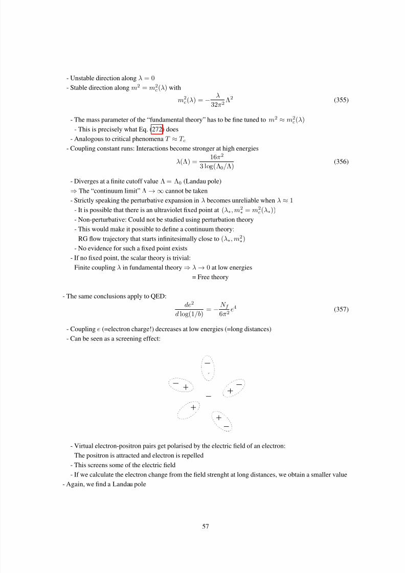
7/30/2019 Aft Notes 12


- Unstable direction along λ = 0

- Stable direction along m2 = m2c(λ) with

m2c(λ) = −λ

32π2 Λ2 (355)

- The mass parameter of the “fundamental theory” has to be fine tuned to m2 ≈ m2c(λ)

- This is precisely what Eq. (272) does

- Analogous to critical phenomena T ≈ T c

- Coupling constant runs: Interactions become stronger at high energies

λ(Λ) =16π2

3 log(Λ0/Λ)(356)

- Diverges at a finite cutoff value Λ = Λ0 (Landau pole)

⇒ The “continuum limit” Λ → ∞ cannot be taken

- Strictly speaking the perturbative expansion in λ becomes unreliable when λ ≈ 1- It is possible that there is an ultraviolet fixed point at (λ∗, m2

∗ = m2c(λ∗))

- Non-perturbative: Could not be studied using perturbation theory

- This would make it possible to define a continuum theory:

RG flow trajectory that starts infinitesimally close to (λ∗, m2∗)

- No evidence for such a fixed point exists

- If no fixed point, the scalar theory is trivial:

Finite coupling λ in fundamental theory ⇒ λ → 0 at low energies

= Free theory

- The same conclusions apply to QED:

de2

d log(1/b)= − N f

6π2e4 (357)

- Coupling e (=electron charge!) decreases at low energies (=long distances)

- Can be seen as a screening effect:

- Virtual electron-positron pairs get polarised by the electric field of an electron:

The positron is attracted and electron is repelled

- This screens some of the electric field

- If we calculate the electron change from the field strenght at long distances, we obtain a smaller value

- Again, we find a Landau pole

57

7/30/2019 Aft Notes 12


e2(Λ) =6π2

N f log(Λ0/Λ)(358)

⇒ QED does not exist as a (perturbative) continuum theory

- Little experimental significance:

If Λ = me (the electron mass), e2(me) = 0.09 and N f = 1, then

Λ0 ≈ 10300 GeV (359)

- QED can only exist as a part of some more fundamental theory (GUT?)

- Most 4D theories have a Landau pole and are trivial

- Main exception: Non-Abelian gauge field theories

9 Advanced Methods

9.1 Dimensional Regularisation

- The cutoff regularisation Λ is concrete and easy to understand but usually impractical

- Multi-loop integrals become very cumbersome

- Incompatible with gauge invariance

- An elegant (but abstract) alternative: Dimensional regularisation

- Consider an Euclidean loop integral I E n (m) in d dimensions (cf Eq. (232)

I E n (m) = E

ddk

(2π)d1

(k2 + m2)n= (2π)d dΩd

∞

0

kd−1dk

(k2 + m2)n(360)

- Using Eq. (236), we can write this as

I E n (m) =2

(4π)d/2Γ(d/2)

∞0

kd−1dk

(k2 + m2)n=

1

(4π)d/2Γ(d/2)

∞0

(k2)d/2−1dk2

(k2 + m2)n(361)

- Now, let us change the integration variable to

x =m2

k2 + m2, (362)

so that the integral becomes

I E n (m) =md−2n

(4π)d/2Γ(d/2) 1

0

xn−d/2−1(1 − x)d/2−1dx (363)

- Now, recall the definition of the beta function 1

0

xα−1(1 − x)β−1dx = B(α, β ) =Γ(α)Γ(β )

Γ(α + β )(364)

- This implies that

I E n (m) =md−2n

(4π)d/2Γ(d/2)

Γ(n − d/2)Γ(d/2)

Γ(n)=

md−2n

(4π)d/2

Γ(n − d/2)

Γ(n)(365)

- The Gamma function Γ(z) has poles at z = 0, −1, −2, . . .

⇒ In 4D, I E n (m) diverges for n = 1, 2, as we have seen before

- But for non-integer d it is always finite!

- We can use Eq. (365) to define the integral for d ∈ R

58

7/30/2019 Aft Notes 12


- In practice, we consider d = 4 − with 1

- For integer l ≥ 0 one has

Γ(−l + /2) =(−

1)l

l!2

+ ψ1(l + 1) + O()

, (366)

where

ψ1(l + 1) = 1 +1

2+ . . . +

1

l− γ, (367)

and γ ≈ 0.577216 is the Euler-Mascheroni constant

- For n ≥ 3, the result is finite (and therefore agrees with momentum cutoff)

- For n = 2, we have

I E 2 (m) =m−

(4π)2−/2Γ(/2) =

1 − log m

(4π)2 1 −

2

log4π 2

− γ + O()

=1

16π2

2

+ log

4π

m2− γ

+ O() (368)

- Comparison this with Eq. (255) shows that the two results agree if we identify

logΛ ↔ 1

+ finite terms (369)

- For n = 1, we find

I E 1 (m) =m2−

(4π)2−/2Γ(−1 + /2) =

m2

(4π)2

1 − log m

1 − 2

log4π(−1)

2

+ 1 − γ

+ O()

= − m2

16π2

2

+ log 4πm2

+ 1 − γ

+ O() (370)

- Comparing this with Eq. (238),

I 1(m) =1

16π2

Λ2 − m2 ln

Λ2

m2

+ O

m2

Λ2

, (371)

we see that the logarithmic terms agree again, but there is no analogue of the quadratic term Λ2

- Generally true: Only log divergences are present

- Simplifies calculations

- Can be sometimes misleading!

- In our results (370) and (368), we seem to have logs of dimensionful quantities- Solutions: In d = 4 − , the coupling has dimensions [λ] =

- Let us therefore write the 4 − dimensional coupling as

λ = λµ, (372)

where [λ] = 0 and [µ] = 1

- Consider a diagram with L loops and V vertices

- The integral is (schematically) proportional to

λV µV

ddk

(2π)d

L(373)

- Using the results in Problem Sheet 4, we find that the number of loops L in a diagram is

59

7/30/2019 Aft Notes 12


L = V − E/2 + 1 (374)

- Using this, our integral becomes

λV µ(L+E/2−1)

ddk

(2π)d

L= µ(E/2−1)λV

µ

ddk

(2π)d

L(375)

- Each loop comes therefore with a factor µ

- Also an overall factor µ(E/2−1), if the whole correlator is finite, this goes to 1 as → 0

- Thus, when going to d = 4 − dimensions, we should replace the integration measure by d4k

(2π)4→ µ

ddk

(2π)d(376)

and we have

I E n (m) = µ E

ddk

(2π)d1

(k2 + m2)n =4πµ2

m2/2

m4−2n

(4π)2

Γ(n−

2 + /2)

Γ(n) (377)

- Then, Eq. (368) becomes

I E 2 (m) =

4πµ2

m2

/21

(4π)2Γ(/2) =

1 + 2

log 4πµ2

m2

(4π)2

2

− γ

+ O()

=1

16π2

2

+ log

4πµ2

m2− γ

+ O() (378)

and Eq. (368) becomes

I E 1 (m) =

4πµ2

m2

/2

m2

(4π)2Γ(−1 + /2) = m2

(4π)2

1 +

2log 4πµ2

m2

(−1)

2

+ 1 − γ

+ O()

= − m2

16π2

2

+ log

4πµ2

m2+ 1 − γ

+ O() (379)

- Finally, consider a massless (m = 0) integral I E n (0)

- If d > 2n, Eq. (365) implies that I E n (0) = 0

- If d < 2n, it diverges

- However, we define it by analytically continuing from high enough d

I E n (0) = 0 for any n and d

- More generally, any scale-free integral is set to vanish

- This procedure is known as dimensional regularisation

- Go to d dimensions by replacing the integrals according to Eq. (376)

- Calculate the integral using Eq. (377)

- If the integral is scale-free, it vanishes

- This way power-law divergences disappear, and log divergences appear as

logΛ2

m2∼ 2

+ log

4πµ2

m2(380)

- To use dimensional regularisation in practice, we need to show that this can be applied to an arbitrary

Minkowskian integral of the form

60

7/30/2019 Aft Notes 12


µ

ddk

(2π)dkµ1 · · · kµm

(k2 − m21)((k + p2)2 − m2

2) · · · ((k + pn)2 − m2n)

(381)

- First, use the identity

1

(k2 − m21)((k + p)2 − m2

2)=

1

0

dx

(k2 + x(2k · p + p2 − m22 + m2

1) − m21)2

=

1

0

dx

((k + xp)2 + x(1 − x) p2 − x(m22 − m2

1) − m21)2

=

1

0

dx

(k2 − ∆)2(382)

where x is known as a Feynman parameter, k = k + xp and

∆ =

−x(1

−x) p2 + x(m2

2

−m2

1) + m21 (383)

- Furthermore, we can write

1

(k2 − ∆)2=

∂

∂ ∆

1

k2 − ∆

(384)

- Using these steps iteratively, we can write the general loop integral (381) in terms of

I µn···µm1 (∆) ≡

µddk

(2π)dkµ1 · · · kµm

(k2 − ∆)n(385)

(Of course, the expression will involve complicated derivatives, and an n − 1-dimensional integral

over Feynman parameters x1, . . . , xn!)

- To deal with the numerator, note that I

µ1···µm

1 (∆) is a symmetric tensor of rank m- Depends only on a scalar quantity ∆, and therefore has to be Lorentz invariant

- The only symmetric tensor available is gµν , and therefore the tensor structure must

be a combination of gµν s only!

- Note, odd number of Lorentz indices ⇒ vanish

- For example,

I µν 1 (∆) = Cgµν , (386)

with some Lorentz scalar C

- Contracting this with gµν , we find

gµν I µν

1 (∆) = µ ddk

(2π)dk2

k2 − ∆ = Cgµν gµν

= dC, (387)

and therefore

I µν 1 (∆) =gµν

dµ

ddk

(2π)dk2

k2 − ∆= gµν

∆

dµ

ddk

(2π)d1

k2 − ∆= −igµν

∆

dI E 1 (∆1/2), (388)

where we used the result that any scale-free integral vanishes

- This way, we can write an arbitrary loop integral as a multi-dimensional integral over Feynman

parameters (which can still be extremely difficult to evaluate!)

- We must do it consistently in d = 4 − dimensions and only take → 0 at the very end

- As an example, let us calculate

61

7/30/2019 Aft Notes 12


I 2( p, m) = µ

ddk

(2π)d1

k2 − m2

1

(k + p)2 − m2(389)

- Using Feynman parameters (382) we can write this as

I 2( p, m) = µ

ddk

(2π)d

1

0

dx

((k + xp)2 + x(1 − x) p2 − m2)2

=

1

0

dx µ

ddk

(2π)d1

(k2 − ∆(x))2, (390)

where

∆(x) = −x(1 − x) p2 + m2 (391)

- Going to Euclidean space, this becomes

I 2( p, m) = i

1

0

dx µ

ddkE (2π)d

1

(k2E + ∆(x))2

= i

1

0

dx I E 2 (∆1/2)

=i

16π2

1

0

dx

2

+ log

4πµ2

∆(x)− γ

=i

16π2

2

+

1

0

dx log4πµ2

−x(1 − x) p2 + m2− γ

(392)

- The integral over x can be done analytically, but leads to a long expression which we omit here

9.2 Minimal Subtraction

- In dimensional regularisation, the one-loop 1PI correlators are

Γ2(k2) =

+

=iλRm2

R

32π2

2

+ log

4πµ2

m2R

+ 1 − γ

+ i

k2δZ − δm2

(393)

and

Γ4 =

+ 3 ×j

+

k

= −iλR

1 − 3λR

32π2

2

+ log

4πµ2

m2R

− γ + f (s,t,u)

− iδλ (394)

- To renormalise the theory, we need to specify how we split the bare parameters to

renormalised parameters and counterterms [see Eq. (303)]

- This split is completely artificial and does not affect the final result

(i.e. relationships between physical observables)

- Earlier we used the “physical” scheme (307)–(309), which has a clear physical interpretation

62

7/30/2019 Aft Notes 12


but is rather clumsy

- Simpler alternative: Minimal subtraction

- Choose counterterms in such a way that they cancel the divergences, but only contain the 1/ pole- Even more convenient: MS (modified minimal subtraction)

- For each pole, include the combination

1

+

1

2

log

4πµ2

M 2− γ

(395)

in the counterterm (because these terms always appear together)

- The mass scale M (renormalisation scale) is arbitrary

- The value does not affect physical results

- Analogous to the energy scales s0, t0 and u0 in Eq. (307)

- One often identifies the scales M = µ, but we keep them separate:

-µ ⇔

regularisation

- M ⇔ renormalisation

- Using MS and Eqs. (393) and (394), we find

δZ = 0

δm2 =λRm2

R

32π2

2

+ log

4πµ2

M 2− γ

δλ =3λ2R

32π2

2

+ log

4πµ2

M 2− γ

(396)

- Substituting these back in Eqs. (393) and (394), we find

Γ2(k2) =iλRm2R

32π2

log

M 2

m2R

+ 1

Γ4 = −iλR

1 − 3λR

32π2

log

M 2

m2R

+ f (s,t,u)

(397)

- We could have even taken a shortcut and simply “subtracted the divergences” from Eqs. (393)

and (394) (and replace µ → M )

- Now m2R and λR do not have any direct physical interpretation

- They are dependent on the renormalisation scale M

- Their scale dependence cancels the explicit M -dependence in Eq. (397)

9.3 Callan-Symanzik Equation

- Physics independent of the renormalisation scale M

⇒ Explicit scale dependence cancelled by the scale dependence of renormalised couplings

- Similarly, bare n-point function GBn ( p1, . . . , pn) is independent of M (for fixed bare couplings)

- On the other hand, the renormalised n-point function GRn ( p1, . . . , pn) is a finite function of the

renormalised couplings and the scale M

GRn ( p1, . . . , pn; m2

R(M ), λR(M ); M ) (398)

- Field renormalisation relates the two

63

7/30/2019 Aft Notes 12


GBn ( p1, . . . , pn) = Z n/2(M )GR

n ( p1, . . . , pn; m2R(M ), λR(M ); M ) (399)

- The M dependence on the RHS must cancel- Let us differentiate GB

n with respect to M

0 = M ∂

∂M GBn

B

= Z n/2(M )

n

M

Z 1/2

∂Z 1/2

∂M

B

+ M ∂m2

R

∂M

B

∂

∂m2R

R

+ M λR

∂M

B

∂

∂λR

R

+ M ∂

∂M

GRn (m2

R, λR; M ), (400)

where |B and |R show whether we keep the bare parameters m2B or λB or the renormalised

parameters m2R, λR fixed when taking the partial derivative

- We then define

γ φ =M

Z 1/2

∂Z 1/2

∂M

B

=1

2Z

∂Z

∂ log M

B

β =∂λR

∂ log M

B

γ 2 =1

m2R

∂m2R

∂ log M

B

(401)

where γ φ is known as the anomalous dimension and β as the beta function

- This leads to the Callan-Symanzik equationM

∂

∂M + β

∂

∂λR+ γ 2m2

R

∂

∂m2R

+ nγ φ

GRn (m2

R, λR; M ) = 0, (402)

which is closely related to our previous RG flow equations but in terms of renormalised quantities

- It shows how the renormalised correlation functions depend on the renormalisation scale M

when the fundamental (“bare”) theory is kept fixed

- This is useful, because we can optimise perturbative calculations by a good choice of M :

- We want our renormalised perturbation theory to converge as fast as possible

- In general, this happens when M is comparable with the characteristic energy scale of the

process we are looking at

- For instance, the scattering amplitude for φφ → φφ scattering is given by Γ4 in Eq. (397):- If we choose M appropriately, the quantum correction becomes small, and λR is

a good approximation of the actual scattering amplitude

- This typically means that M is close to the most relevant energy scales for the process

- The beta function β tells how the interaction strength depends on the characteristic energy scale

- According to Eq. (303), we can write the renormalised parameters as

64

7/30/2019 Aft Notes 12


Z (M ) = 1 + δZ (M )

λR

(M ) = Z (M )2λB −

δλ(M )

m2R(M ) = Z (M )m2

B − δm2(M ) (403)

- This means that to leading order we have

γ φ =1

2Z

∂δZ

∂ log M

B

≈ 1

2

∂δZ

∂ log M

R

β = 2ZλB∂Z

∂ log M

B

− ∂δλ

∂ log M

B

≈ 4λRγ φ − ∂δλ

∂ log M

R

γ 2 =m2B

m2R

∂Z

∂ log M

B

− 1

m2R

∂δm2

∂ log M

B

≈ 2γ φ − ∂δm2

∂ log M

R

(404)

- In the M S scheme, we obtain the counterterms in terms of the renormalised couplings

- The counterterms are are proportional to

2

+ log

4π2µ2

M 2− γ, (405)

with no other (explicit) M dependence

- The coefficients γ φ, β and γ 2 are therefore M -independent

- In fact, we can write the counterterms as

δZ = −γ φ 2

+ log

4π2µ2

M 2− γ

δm2 =

1

2γ 2 − γ φ

m2R

2

+ log

4π2µ2

M 2− γ

δλ =

1

2β − 2λRγ φ

2

+ log

4π2µ2

M 2− γ

(406)

- Comparing with Eq. (396), we find

γ φ = 0

β =3λ2R

16π2

γ 2 =

λR16π2 (407)

- Compare with Eq. (354):

dλ

d log(1/b)= − 3λ2

16π2= −β (λ) + O(λ3) (408)

- The leading term is generally the same:

65

7/30/2019 Aft Notes 12


β =∂λR

∂ log M B = − ∂λR∂λB M

∂λB∂ log M R

=∂λR∂λB

M

∂λB∂ logΛ

R

≈ ∂λB∂ log Λ

R

=∂λB

∂ log1/b

R

(409)

where we used the fact that between the cutoff and dimensional regularisation, the divergences

correspond to each other as

log Λ ∼ logµ

M (410)

and that to leading order λR = λB

- Higher orders depend on the renormalisation scheme

- Leading order is enough to determine the nature of the Gaussian fixed point

and therefore whether the theory is trivial or asymptotically free

10 Renormalisation of QCD

10.1 Counterterms

- The gauge-fixed Lagrangian (152) has six parameters:

- Three field normalisations: Aµ, c and ψ

- Parameters: g, ξ and m

- Do we need to include more terms to renormalise the theory?- Generally all terms compatible with symmetries

- Gauge invariance is broken by gauge fixing, so it cannot protect the Lagrangian

- The gauge fixed theory has a more complicated BRST (Becchi-Rouet-Stora-Tyutin) symmetry

- Introduce auxiliary field Ba with Lagrangian

LB =1

2ξBaBa + Ba∂ µAa

µ (411)

- Integrating over Ba gives the gauge fixing term DBei

ddxLB = const × ei

ddx(− 1

2ξ (∂ µAaµ)2) (412)

- We can therefore replace in the Lagrangian (152)− 1

2ξ (∂ µAa

µ)2 → 1

2ξBaBa + Ba∂ µAa

µ (413)

- The resulting Lagrangian has a peculiar BRST symmetry

66

7/30/2019 Aft Notes 12


Aaµ → Aa

µ + Dacµ cc

ψi →

ψi −

igtaij

caψj

ca → ca +1

2gf abccbcc

ca∗ → ca∗ + Ba

Ba → Ba (414)

- This symmetry does not allow any new terms, and therefore it is enough to consider

Lagrangians of the form (152)

- All four interactions have coupling g (or g2)

- Related by gauge invariance, even in quantum theory

- We treat them as independent at first

- To set up renormalised perturbation theory, we first rescale the fields by renormalisation constants:

Aaµ → Z

1/2A Aa

µ, ca → Z 1/2c c2, ψi → Z

1/2ψ ψi (415)

- The Lagrangian (152) becomes

L = −1

4Z A(∂ µAa

ν − ∂ ν Aaµ)(∂ µAaν − ∂ ν Aaµ) − 1

2

Z Aξ B

(∂ µAaµ)2

+Z c∂ µca∗∂ µca + Z ψψi (i / ∂ − mB) ψi

+1

2gBZ

3/2A f abc(∂ µAa

ν − ∂ ν Aaµ)AbµAcν − 1

4g2BZ 2Af abcf adeAb

µAcν A

d µAe ν

−gBZ cZ 1/2A ∂ µca∗f abcAb

µcc − gBZ ψZ 1/2A γ µαβtaijAa

µψiαψjβ , (416)

where we have also added the subscripts “B” to the parameters to indicate they are bare ones

- We define renormalised parameters by introducing multiplicative renormalisation constants

Z Aξ B

=Z ξξ

Z ψmB = Z mm

Z 3/2A gB = Z 3g

Z 2Ag2B = Z 4g2

Z cZ 1/2A gB = Z 1g

Z ψZ 1/2A gB = Z 2g (417)

- Note that the renormalisation constants Z 1, Z 2, Z 3 and Z 4 are related to each other

- In terms of the renormalised fields and parameters, the Lagrangian is therefore

67

7/30/2019 Aft Notes 12


L = −1

4Z A(∂ µAa

ν − ∂ ν Aaµ)(∂ µAaν − ∂ ν Aaµ) − 1

2

Z ξξ

(∂ µAaµ)2

+Z c∂ µca∗∂ µca + ψi

iZ ψ / ∂ − Z mm

ψi

+1

2Z 3gf abc(∂ µAa


4Z 4g2f abcf adeAb

µAcν A

dµAe ν

−Z 1g∂ µca∗f abcAbµcc − Z 2gγ µαβtaijAa

µψiαψjβ , (418)

- Next we write the renormalisation constants Z X in terms of counterterms, Z X = 1 + δZ X

- This gives

L = −1

4(∂ µAa

ν − ∂ ν Aaµ)(∂ µAaν − ∂ ν Aaµ) − 1

2ξ (∂ µAa

µ)2

+∂ µca∗∂ µca + ψi i / ∂

−mψi

+1

2gf abc(∂ µAa


4g2f abcf adeAb

µAcν A

dµAe ν

−g∂ µca∗f abcAbµcc − gγ µαβtaijAa

µψiαψjβ

−1

4δZ A(∂ µAa

ν − ∂ ν Aaµ)(∂ µAaν − ∂ ν Aaµ) − 1

2

δZ ξξ

(∂ µAaµ)2

+δZ c∂ µca∗∂ µca + ψi

iδZ ψ / ∂ − δZ mm

ψi

+1

2δZ 3gf abc(∂ µAa


4δZ 4g2f abcf adeAb

µAcν A

d µAe ν

−δZ 1g∂ µca∗f abcAbµcc − δZ 2gγ µαβtaijAa

µψiαψjβ (419)

- The propagators were given in Eqs. (218)–(220)

- The interaction vertices are Eqs. (224), (226), (228) and (230), together with the counterterm vertices

68

7/30/2019 Aft Notes 12


l

Aaµ(k) Ab

ν (−k) ↔ −iδ ab δZ A k2gµν − kµkν − δZ ξ

ξ kµkν

m ψjβ(k) ψiα(k) ↔ iδ ij (δZ ψ / k − δZ mm)αβ

n cb∗(k) ca(k) ↔ −iδ abδZ ck2

o

Aaµ(k1)

Abν (k2) Ac

ρ(k2)

↔ gδZ 3f abc [gµν (kρ2 − kρ1 ) + gνρ(kµ3 − kµ2 ) + gµρ(kν 1 − kν 3 )]

Aaµ Ab

ν

Acρ Ad

λ

↔ −ig2δZ 4

f abef cde


+f acef bde


+f adef bce gµν gρλ − gµρgνλ

Abµ(k2)

ca∗(k1) cb(k3)

↔ δZ 1gf abckµ1

Aaµ

ψiα ψjβ

↔ −iδZ 2gγ µαβtaij (420)

- To determine the counterterms, we have to find out which correlator gets a tree-level contribution

from each counterterm

69

7/30/2019 Aft Notes 12


δZ A, δZ ξ ↔

δZ c ↔

δZ ψ, δZ m ↔

δZ 1 ↔

δZ 2 ↔

δZ 3 ↔

δZ 4 ↔

(421)

- We need to compute all the two-point functions, but because Z 1–Z 4 are related, it is enough

to compute one of the last four correlators

- We choose the quark-gluon interaction δZ 2, because it consists of fewer diagrams than

the gluon-gluon interactions, and it corresponds to a real physical process unlike

the ghost-gluon interaction

⇒ We need four correlation functions to determine the six counterterms

10.2 Correlation Functions

10.2.1 Gluon

- We start by looking at the gluon two-point function

70

7/30/2019 Aft Notes 12


z

=

+

|

+

+

~

+

(422)

- The quark loop is

p + k

p

Aaµ(k) Ab

ν (−k)i α

j β

γ i

δ j

=1

2!× (−1) × 2 ×

−igγ µαβtaij

−igγ ν γδ tbji×

×µ

dd p

(2π)d

i

/ p + / k − m

δα

i

/ p − m

βγ

= g2tr tatbµ

dd p

(2π)dTr

i

/ p + / k − m

γ µ

i

/ p − m

γ ν ,(423)

where tr is a trace over colour indices ij and Tr over spinor indices αβ

- To proceed, we have to recall some identities involving gamma matrices

γ µ, γ ν = 2gµν ⇒ 1

/ p − m=

/ p + m

p2 − m2

Tr γ µγ ν = 12 Tr γ µ, γ ν = gµν Tr 1 = 4gµν

Tr γ µγ ν γ ρ = 0

Tr γ µγ ν γ ργ λ = 4

gµν gρλ + gµλgνρ − gµρgνλ

(424)

- Thus, we have

= −g2tr tatbµ

dd p

(2π)dTr ( / p + / k + m)γ µ( / p − m)γ ν

((k + p)2 − m2)( p2 − m2)

= −g2tr tatb 1

0

dxµ dd p

(2π)dTr ( / p + / k + m)γ µ( / p − m)γ ν

(( p + xk)2

−∆(x))2

, (425)

where on the second line we have used the Feynman parameter trick (382) and defined

∆(x) = −x(1 − x)k2 + m2 (426)

- We shift the integration variable p + xk → p,

71

7/30/2019 Aft Notes 12


= −g2tr tatb 1

0

dxµ dd p

(2π)dTr ( / p + (1 − x) / k + m)γ µ( / p − x / k − m)γ ν

( p2

−∆(x))2

(427)

= −g2tr tatb 1

0

dxµ

dd p

(2π)d( p + (1−x)k)ρ( p − xk)λTrγ ργ µγ λγ ν + m2Tr γ µγ ν

( p2 − ∆(x))2

= −g2tr tatb 1

0

dxµ

dd p

(2π)d( pρ pλ − x(1−x)kρkλ)Trγ ργ µγ λγ ν + m2Tr γ µγ ν

( p2 − ∆(x))2,

where in the last step we used the fact that terms with one power of p in the numerator vanish

- As in Eq. (388), we have

µ

dd p

(2π)d pρ pλ

( p2 − ∆)2=

gρλd

µ

dd p

(2π)d p2

( p2 − ∆)2=

gρλd

(I 1(∆) + ∆I 2(∆)) , (428)

where

I n(∆) = µ

dd p

(2π)d1

( p2 − ∆)n(429)

- The values of the integrals are given by Eq. (365)

I 1(∆) = −i∆d/2−1

(4π)d/2Γ(1 − d/2)

I 2(∆) = i∆d/2−2

(4π)d/2Γ(2 − d/2) (430)

- The Gamma function satisfies zΓ(z) = Γ(z + 1), which implies

(2 − d)I 1(∆) = −2i∆d/2−1

(4π)d/2

1 − d

2

Γ(1 − d/2) = −2i

∆d/2−1

(4π)d/2Γ(2 − d/2) = −2∆I 2(∆) (431)

and further

µ

dd p

(2π)d pρ pλ

( p2 − ∆)2=

gρλd

2

d − 2∆I 2(∆) + ∆I 2(∆)

=

gρλd − 2

∆I 2(∆) (432)

- Using Eqs. (424), we find

= −4g2tr tatb

1

0

dx

gρλ

d

−2

∆I 2(∆) − x(1 − x)kρkλI 2(∆)

×

× gµρgνλ + gµλgνρ − gµν gρλ

+m2gµν I 2(∆)

= −4g2tr tatb 1

0

dx

2 − d

d − 2gµν ∆I 2(∆)

−x(1 − x)

2kµkν − k2gµν

I 2(∆) + m2gµν I 2(∆)

= −4g2tr tatb 1

0

dx−∆ + x(1− x)k2 + m2

gµν − 2x(1−x)kµkν

I 2(∆)

= −4g2tr tatb 1

0

dx 2x(1−x)

k2gµν − kµkν

I 2(∆), (433)

where we used ∆ = m2 − x(1 − x)k2

72

7/30/2019 Aft Notes 12


- Near four dimensions, when d = 4 − , we have

I 2(∆) ≈ i

16π2 2

+ finite , (434)

and therefore

= − 4ig2

16π2tr tatb

k2gµν − kµkν

2

+ finite

1

0

dx 2x(1 − x)

= − ig2

16π2tr tatb

4

3

k2gµν − kµkν

2

+ finite

(435)

- We could calculate the finite part, but for MS renormalisation it is not needed

- The group factor tr tatb ≡ C (r)δ ab depends on the quark representation r

- For the fundamental representation (our case), Eq. (123) gives C (r) = 1/2

- For N f fermion species, the total result is

= − ig2

16π2

4

3N f C (r)δ ab

k2gµν − kµkν

2

+ finite

(436)

- The second diagram in Eq. (422) gives

=

ig2

16π2f acdf bcd

25

12− ξ

2

k2gµν −

17

6− ξ

kµkν

2

+ finite

= ig

2

16π2 C 2(G)δ ab

2512 − ξ 2

k2gµν − kµkν

+−34 + ξ 2

kµkν

×

×

2

+ finite

, (437)

where we have written f acdf bcd = C 2(G)δ ab in terms of the quadratic Casimir invariant

of the adjoint representation (for SU(N ), C 2(G) = N )

- The third diagram is

= 0, (438)because the integral is scale-free

- The ghost loop (4th diagram) gives

=

ig2

16π2f acdf bcd

1

12k2gµν +

1

6kµkν

2

+ finite

=ig2

16π2C 2(G)δ ab

1

12

k2gµν − kµkν

+

1

4kµkν

2

+ finite

, (439)

- Finally, the counterterm diagram gives

73

7/30/2019 Aft Notes 12


= −iδZ A

k2gµν − kµkν

− iδZ ξ

ξ kµkν (440)

- Putting all of these together, we find

=

ig2

16π2δ ab

−4

3N f C (r) +

13

6− ξ

2

C 2(G)

k2gµν − kµkν

+

ξ − 1

2C 2(G)kµkν

2

+ finite

−iδZ A

k2gµν − kµkν − i

δZ ξξ

kµkν (441)

- Following the MS scheme, we must therefore choose

δZ A =g2

16π2

−4

3N f C (r) +

13

6− ξ

2

C 2(G)

2

+ log

4πµ2

M 2− γ

δZ ξ

ξ =

g2

16π2

ξ − 1

2C 2(G)

2

+ log

4πµ2

M 2− γ

(442)

- There are some interesting points to note:

- The counterterms depend on ξ , but that is not a problem because they are not physical observables

- The gauge fixing parameter ξ gets renormalised:

It is therefore not consistent to simply fix its value to something convenient

10.2.2 Quark

- The quark two-point function consists of only two diagrams

=

+

(443)

- The loop diagram is

p + k

− p

ψiα(k) ψjβ (k)a µ

i l

ν a

l j

=−igγ µγαtali

−igγ ν βδ tajl×

×µ

dd p

(2π)dDµν F ( p)S δγ F ( p + k)

= −g2(tata)jiµ

dd p

(2π)dDµν F ( p)

γ ν S δγ F ( p + k)γ µ

βα

(444)

74

7/30/2019 Aft Notes 12


- Note that the order of the matrices is opposite to the propagation of the quark

- We have here the quadratic Casimir of the quark representation

(ta

ta

)ij = C 2(r)δ ij (445)

- For the fundamental representation in SU(N ), C 2(r) = (N 2 − 1)/2N

- Doing the algebra and evaluating the integral, one finally obtains

=ig2

16π2δ ijC 2(r) (ξ / k − (3 + ξ )m)βα

2

+ finite

(446)

- The counterterm diagram gives

= i (δZ ψ / k

−δZ mm) δ ij (447)

- In the M S scheme, we therefore have

δZ ψ = − g2

16π2C 2(r)ξ

2

+ log

4πµ2

M 2− γ

δZ m = − g2

16π2C 2(r)(3 + ξ )

2

+ log

4πµ2

M 2− γ

(448)

10.2.3 Ghost

- The ghost two-point function consists of

=

+

, (449)

where

=ig2

16π2δ abC 2(G)

3 − 5ξ

4k2

2

+ finite

(450)

and

= −iδ abk2δZ c (451) -Therefore, we have

δZ c =g2

16π2C 2(G)

3 − 5ξ

4

2

+ log

4πµ2

M 2− γ

(452)

75

7/30/2019 Aft Notes 12


10.2.4 Quark-gluon coupling

- To compute δZ 2, we need the quark-gluon interaction

Aaµ(q )

ψiα(k) ψjβ(k + q )

=

+

+

, (453)

where

= −ig3

16π2

C 2(r) −1

2 C 2(G)

ξt

a

jiγ

µ

βα2

+ finite

, (454)

= − ig3

16π2C 2(G)

3(1 + ξ )

4tajiγ µβα

2

+ finite

, (455)

and

= −iδZ 2gγ µβαtaji (456)

- This means that the counterterm is

δZ 2 =g2

16π2

−3(1 + ξ )

4C 2(G) − ξC 2(r) +

ξ

2C 2(G)

2

+ log

4πµ2

M 2− γ

= − g2

16π2

3

4C 2(G) +

1

4C 2(G) + C 2(r)

ξ

2

+ log

4πµ2

M 2− γ

(457)

10.2.5 Summary

- In summary, the values of the counterterms are

76

7/30/2019 Aft Notes 12


δZ A =g2

16π2 13

6− ξ

2C 2(G) − 4

3N f C (r)

2

+ log

4πµ2

M 2− γ

δZ ψ = − g2

16π2C 2(r)ξ

2

+ log

4πµ2

M 2− γ

δZ c =g2

16π2C 2(G)

3 − 5ξ

4

2

+ log

4πµ2

M 2− γ

δZ ξ

ξ =

g2

16π2

ξ − 1

2C 2(G)

2

+ log

4πµ2

M 2− γ

δZ m = − g2

16π2C 2(r)(3 + ξ )

2

+ log

4πµ2

M 2− γ

δZ 2 = − g2

16π2

3

4C 2(G) +

1

4C 2(G) + C 2(r)

ξ

2

+ log

4πµ2

M 2− γ

(458)

10.3 Beta Function

- We can now compute the QCD beta function

β (g) = M ∂g

∂M

B

(459)

- In terms of the bare coupling and the counterterms, the renormalised coupling is

g =

Z ψZ 1/2A

Z 2 gB =

1 + δZ ψ +

1

2 δZ A − δZ 2

gB + O(g5

B) (460)

- Therefore, we have

β (g) = 2g

∂δZ ψ

∂ log M 2+

1

2

∂δZ A∂ log M 2

− ∂δZ 2∂ log M 2

= 2g

g2

16π2ξC 2(r)

−1

2

g2

16π2

13

6− ξ

2

C 2(G) − 4

3N f C (r)

−g2

16π2 3

4

C 2(G) + 1

4

C 2(G) + C 2(r) ξ =

2g3

16π2

(ξ − ξ ) C 2(r) +

−13

12+

ξ

4− 3

4− ξ

4

C 2(G) +

2

3N f C (r)

=g3

16π2

−11

3C 2(G) +

4

3N f C (r)

(461)

- The gauge (ξ ) dependence has now disappeared

- For SU(N ) and fundamental quarks we have C 2(G) = N and C (r) = 1/2, and therefore

β (g) =g3

16π2

−11N

3+

2

3N f

(462)

- If N f < (11/2)N , the beta function is negative

77

7/30/2019 Aft Notes 12


⇒ The interaction gets weaker at higher energies (=asymptotic freedom)

- This is precisely what deep inelastic scattering results showed already in 1970s

- Interaction becomes strong at low energies: This is why we cannot see individual quarks and gluons- This calculation gave Gross, Politzer and Wilczek the 2004 Nobel prize

10.4 Renormalisation Group Flow

- Consider the flow in the Wilsonian approach (Section 8.3)

- Use g and m/Λ as coordinates

- How does the effective bare coupling g change as we lower the cutoff?

- It is given by the equation

dg

d logΛ

= β (g) =g3

16π2 −

11N

3

+2

3

N f (463)

- If N f < (11/2)N , β (g) < 0, and g is marginally unstable

- This is easy to solve

1

g2=

1

8π2

11N

3− 2

3N f

log

Λ

ΛQCD, (464)

where ΛQCD is an integration constant

0 0.5 1g

0

1

m / Λ

- Because the beta function is negative (not positive as in QED or scalar theory), the flow is directed

away from the Gaussian fixed point (circle)

- Continuum limit Λ → ∞ corresponds to following the flow trajectory backwards- We can go arbitrarily far ⇒ The theory has a continuum limit (unlike QED or scalar theory)

- Following the flow towards low energies, g diverges at Λ = ΛQCD

- Analogue of the Landau pole but at low energies

- Physics does not really become singular:

It just becomes non-perturbative, so our assumptions fail

- Below ΛQCD we need a different effective theory:

- The relevant degrees of freedom are protons and neutrons, not quarks and gluons

- In a sense, the flow does not actually hit g = ∞ but it leaves the two-dimensional plane

- The appropriate theory is known as chiral perturbation theory

- This explains why we don’t see massless gluons or individual quarks

- The hadron masses given by ΛQCD

78

7/30/2019 Aft Notes 12


- Account for most of the mass of everyday objects

- Nothing to do with the Higgs field!

- In the Callan-Symanzik approach, the same equation tells how the renormalised coupling depends on M ,1

g2R

=1

8π2

11N

3− 2

3N f

log

M

ΛQCD(465)

- Note that gR depends only on how far above ΛQCD we are:

- There is no free dimensionless parameter

- LEP:

αs(M Z ) =g2(M Z )

4π= 0.1176 ± 0.002 ⇒ ΛQCD ≈ 250 GeV (466)

- Compare with classical theory

- Classical Yang Mills:- scale-invariant

- interaction strength is given by dimensionless parameter g

- Quantised Yang-Mills:

- scale-dependent

- interaction strength given by dimensionful scale ΛQCD

- If we assume the quarks are massless, ΛQCD is the only scale in the theory

⇒ There is nothing we could compare it with

- This means that Yang-Mills or QCD with massless quarks is a unique theory:

There is no free parameter that we could vary

79

7/30/2019 Aft Notes 12


Index

1PI correlator, 38

anomalous dimension, 64

asymptotic freedom, 78

beta function, 64

BHPZ theorem, 49

BRST symmetry, 66

Casimir invariant, 73

coarse-graining, 50

conformal field theory, 55connected correlator, 38

continuum limit, 57

counterterm, 47

critical phenomena, 57

dimensionality, 44

effective action, 50

effective field theory, 50

Faddeev-Popov ghost, 23

Feynman diagram, 26

Feynman gauge, 24

Feynman parameter, 61

Feynman propagator, 12

Feynman rules, 30

fixed point, 55

gauge condition, 20

gauge fixing parameter, 22

gauge invariance, 17

Gaussian fixed point, 55

generating function, 10

Grassmann algebra, 14

Grassmann numbers, 14

marginal operator, 56

modified minimal subtraction (MS ), 63

non-renormalisable, 45

one-particle irreducible, 38

relevant operator, 55

renormalisable, 45

renormalisation constant, 67

renormalisation group transformation, 54

renormalisation scale, 63renormalisation scheme, 48

renormalised coupling, 41

renormalised mass, 42

running coupling, 57

scale-free integral, 60

scattering cross section, 40

structure constants, 19

superficial degree of divergence, 44

superrenormalisable, 45

symmetry factor, 29

trivial theory, 57

ultraviolet cutoff, 36

Wick rotation, 49

Aft Notes 12

Documents

Transcript of Aft Notes 12