Aerothermodynamic Calculations on X-34 at Mach 6 Wind ... · PDF fileAerothermodynamic...
26
NASA/TM 1999 208998 Aerothermodynamic Calculations on X-34 at Mach 6 Wind Tunnel Conditions William A. Wood Langley Research Center, Hampton, Virginia February 1999 https://ntrs.nasa.gov/search.jsp?R=19990018442 2018-05-22T01:33:00+00:00Z
Transcript of Aerothermodynamic Calculations on X-34 at Mach 6 Wind ... · PDF fileAerothermodynamic...

NASA/TM 1999 208998
Aerothermodynamic Calculations onX-34 at Mach 6 Wind TunnelConditions
William A. Wood
Langley Research Center, Hampton, Virginia
February 1999
https://ntrs.nasa.gov/search.jsp?R=19990018442 2018-05-22T01:33:00+00:00Z

The NASA STI Program Office ... in Profile
Since its founding, NASA has been dedicated
to the advancement of aeronautics and spacescience. The NASA Scientific and Technical
Information (STI) Program ONce plays a keypart in helping NASA maintain this
important role.
The NASA STI Program Office is operated by
Langley Research Center, the lead center forNASA's scientific and technical information.
The NASA STI Program Office providesaccess to the NASA STI Database, the
largest collection of aeronautical and spacescience STI in the world. The Program Officeis also NASA's institutional mechanism for
disseminating the results of its research anddevelopment activities. These results are
published by NASA in the NASA STI Report
Series, which includes the following reporttypes:
TECHNICAL PUBLICATION. Reports of
completed research or a major significantphase of research that present the results
of NASA programs and include extensivedata or theoretical analysis. Includes
compilations of significant scientific andtechnical data and information deemed
to be of continuing reference value. NASAcounterpart and peer-reviewed formal
professional papers, but having lessstringent limitations on manuscriptlength and extent of graphic
presentations.
TECHNICAL MEMORANDUM.
Scientific and technical findings that arepreliminary or of specialized interest,
e.g., quick release reports, workingpapers, and bibliographies that containminimal annotation. Does not contain
extensive analysis.
CONTRACTOR REPORT. Scientific and
technical findings by NASA-sponsored
contractors and grantees.
CONFERENCE PUBLICATION.
Collected papers from scientific andtechnical conferences, symposia,
seminars, or other meetings sponsored orco-sponsored by NASA.
SPECIAL PUBLICATION. Scientific,
technical, or historical information fromNASA programs, projects, and missions,
often concerned with subjects havingsubstantial public interest.
TECHNICAL TRANSLATION. English-
language translations of foreign scientificand technical material pertinent toNASA's mission.
Specialized services that complement the STIProgram Office's diverse offerings include
creating custom thesauri, building customizeddatabases, organizing and publishingresearch results.., even providing videos.
For more information about the NASA STI
Program Office, see the following:
Access the NASA STI Program HomePage at http://www.sti, nasa.gov
E-mail your question via the Internet to
Fax your question to the NASA STI HelpDesk at (301) 621 0134
Phone the NASA STI Help Desk at (301)621 0390
Write to:
NASA STI Help Desk
NASA Center for AeroSpace Information7121 Standard Drive
Hanover, MD 21076-1320

NASA/TM 1999 208998
Aerothermodynamic Calculations onX-34 at Mach 6 Wind TunnelConditions
William A. Wood
Langley Research Center, Hampton, Virginia
National Aeronautics andSpace Administration
Langley Research CenterHampton, Virginia 23681-2199
February 1999

Available from:
NASA Center for AeroSpace Information (CASI)7121 Standard Drive
Hanover, MD 21076 1320
(301) 621-0390
National Technical Information Service (NTIS)
5285 Port Royal Road
Springfield, VA 22161 2171
(703) 605-6000

Abstract
The effects of Reynolds number and turbulence on surface heat-transfer rates
are numerically investigated for a 0.015 scale X-34 vehicle at wind tunnel con-
ditions. Laminar heating rates, non-dimensionalized by Fay-Riddell stagnation
heating, do not change appreciably with an order of magnitude variation in
Reynolds number. Modeling a turbulent versus laminar boundary layer at the
same Reynolds number increases the windside heating by a factor of four, por-
tions on the leeside by a factor of two, and causes a 30 percent increase in
wing leading edge heating. A discrepancy between laminar and turbulent heat-
ing trends on the windside centerline is explained by the presence of attached
windside vortices in the laminar solutions, structures that are inhibited by the
turbulence modeling.
Nomenclature
CD
CLCMCpi, j, k
L/DM
QReT
V
x,y,z
P
Drag coefficientLift coefficient
Pitching-moment coefficientPressure coefficient
Streamwise, circumferential, and body-normal computational indices
Lift-to-drag ratioMach number
Nondimensionalized heat-transfer rate
Reynolds number based on model length
Temperature, K
Velocity magnitude, m/s
Cartesian coordinates, m
Density, kg/m 3
Subscripts
oc Freestream
1 Introduction
X-3411, 2] is a NASA program with Orbital Sciences Corporation as the prime
contractor[3]. The X-34 purpose is to demonstrate next-generation reusablelaunch vehicle technologies. The X-34 program goals are to build a flight vehicle
with first-flight in 1999, demonstrating fully-reusable operation with efficient
ground support and quick turn-around times. It is anticipated that a more
aircraft-like operational capability will lead to greatly reduced launch costs over
current space transportation systems.
The X-34 will be air-launched from an L 1011 airplane. Landing will be
on a conventional runway. An artist's sketch of the flight sequence, taken from

Coast
aurnou_'__ DescentLaunch L-1011 / _\
carrier aircraft _
___. / Ascent _
Ignition
I Down range landing
Recovery
Landing _=_
Runway91
Figure 1:X-34 flight sequence, taken from Ref. [4].
Ref. [4], is depicted in Fig. 1. Flight tests will focus on both low and high-speed
performance, with a peak Mach number of 8. Peak heating is expected to occur
around Mach 6, with turbulent flow.
NASA Langley has participated in a task agreement with Orbital Sciences
to assist in the prediction of the X-34 aerothermodynamic environment and the
analysis of the aerothermal design of the vehicle. To this end, a series of wind
tunnel experiments and numerical simulations have been performed. Berry et
a/[5] and Merski[6] conducted a matrix of ground-based experimental heating
tests using the thermographic phosphor technique at Mach 6 and Mach 10 for
both laminar and turbulent flows. Kleb et al[4, 7] and Riley et a/J8] have com-
puted heating rates at flight conditions covering Mach 3 7, with most of thecalculations for turbulent flow. Comparisons between the experimental heat-
ing data, extrapolated to flight values, and computations has been presented in
Refs. [4]-[7].The present study seeks to provide overlap between the numerical and exper-
imental data sets by performing computational simulations of the X-34 vehicle
at wind tunnel conditions. The primary emphasis is on the detailed definition of
the thermal environment, though vehicle aerodynamic coefficients and flowfield
features are also presented.
2 Configuration
The geometry is a 0.015 scale model of the X-34 outer mold lines, including the
thermal protection covering, truncated at the body-flap hinge line. The body
flap and rocket nozzle were omitted from the calculations, with an assumed base
pressure equal to freestream static pressure. A depiction of the model used in
this study is presented in Fig. 2.
The model length is 0.246 m. For convenience, moments are taken about the
nose tip, the reference length for aerodynamic coefficients is the model length,
and the reference area is the model length squared.
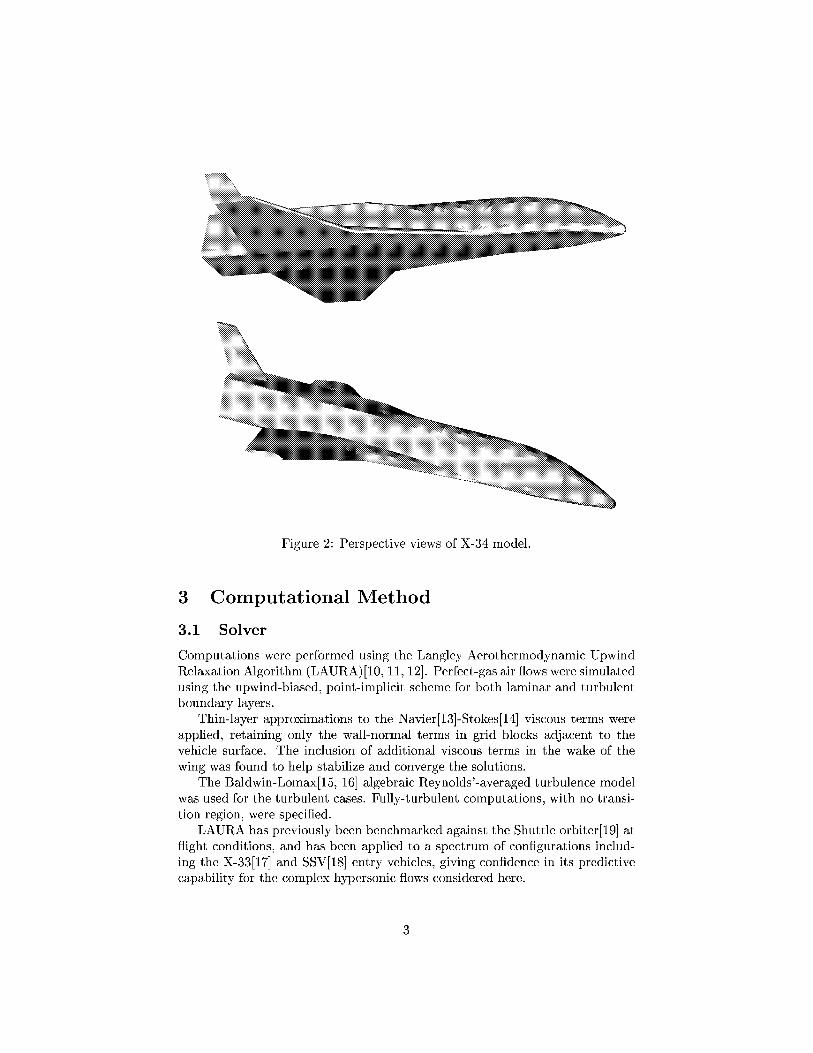
Figure2: PerspectiveviewsofX-34model.
3 Computational Method
3.1 Solver
Computations were performed using the Langley Aerothermodynamic Upwind
Relaxation Algorithm (LAURA)[10, 11, 12]. Perfect-gas air flows were simulated
using the upwind-biased, point-implicit scheme for both laminar and turbulentboundary layers.
Thin-layer approximations to the Navier[13]-Stokes[14] viscous terms wereapplied, retaining only the wall-normal terms in grid blocks adjacent to thevehicle surface. The inclusion of additional viscous terms in the wake of the
wing was found to help stabilize and converge the solutions.
The Baldwin-Lommx[15, 16] algebraic Reynolds'-averaged turbulence model
was used for the turbulent cases. Fully-turbulent computations, with no transi-
tion region, were specified.
LAURA has previously been benchmarked against the Shuttle orbiter[19] at
flight conditions, and has been applied to a spectrum of configurations includ-
ing the X-33[17] and SSV[18] entry vehicles, giving confidence in its predictive
capability for the complex hypersonic flows considered here.
Wing
:_iiiiiiiiii:_iiiiiliiiii_ Ciiiiiiiiiiiiii_
iiiiiiiiiiiiiiii rank Nose
Aftbody _iiiiiiiiiiiiiiiiii__ Strake \
Forebody\...... .......' -0.'25 -0'.2 -0.'15 -0'.1 -0.'05
z,m
Figure 3: Streamwise blocking for circumferential coarsening.
3.2 Grid
The structured computational mesh contains 369 points in the streamwise di-
rection, 305 points around the vehicle from the windside to leeside symmetry
planes, and 65 points normal to the surface. An additional 72 x 16 x 80 grid was
inserted behind the wing trailing edge. Details of the grid generation process,
including grid-quality assessments, have been reported by Alter[9].The domain was partitioned into six streamwise blocks, referred to as the
nose (i=1 21), forebody (i=21 61), strake (i=61 133), crank (i=133 225), wing
(i=225 297), and aftbody (i=297 369). The number of circumferential points,
305, was chosen to resolve all surface features around the wings. Fewer points
are needed to resolve the geometrically simpler cross sections forward of the
wings. Hence, the strake and crank blocks were coarsened, in the circumferential
direction only, by a factor of two, the forebody by a factor of four, and the nose
by a factor of eight. A planform view of the configuration with breaklines for
the six streamwise blocks is shown in Fig. 3.
The domain was further split into a total of 31 blocks to reduce mere-
ory requirements. With this mesh and blocking scheme, the solution required
530 MWords of memory on a 16-processor Cray C-90. Grid adaption was per-
formed to align the mesh with the bow shock and to cluster points in the bound-
ary layer. Solutions required approximately 200 CPU hours each on the C-90.
4 Cases
Two sets of freestream conditions simulate the perfect gas flow of air in a Mach-6wind tunnel. The core flow is assumed to be uniform.
For the low Reynolds number case: Vo_ = 927 m/s, T_ = 60.7 K, andp_ = 0.0160 kg/m 3. This corresponds to M_ = 5.94 and Re = 0.9 x 10⁶ based
on model length. A laminar solution was computed at these conditions.
For the high Reynolds number case: Vo_ = 954 m/s, T_ = 62.4 K, andp_ = 0.1136 kg/m 3. This corresponds to M_ = 6.02 and Re = 6.4 x 10⁶. Both
laminar and turbulent solutions were computed at these conditions.
The wall temperature is held constant at 300 K and the angle of attack is

Re x 10 -_ Boundary layer CD CL CM L/D0.9 laminar 0.003467 0.008280 -0.005813 2.396.4 laminar 0.003180 0.008358 -0.005807 2.63
6.4 turbulent 0.003410 0.008472 -0.005932 2.48
Table 1: Aerodynamic coefficients.
15 deg for all cases. Heating results for the high Reynolds number case are nor-
realized by 405 kW/m 2 and for the low Reynolds number case by 128 kW/m 2.
These values are determined by a Fay and Riddell[20] stagnation point calcula-
tion on a sphere of radius 2.5 mm at the same freestream conditions.
5 Results
5.1 Aerodynamics
To illustrate the effects of Reynolds number and turbulence on the static longi-
tudinal aerodynamic characteristics, lift, drag, and pitching-moment coefficients
are presented in Table 1. Recall that the X-34 configuration modeled in this
study lacks the aft body flap and bell nozzle present on the true vehicle.
Increasing Reynolds number is seen to reduce CD and increase C5, leading
to a 10 percent increase in lift-to-drag ratio. Forcing a turbulent boundary layer
at the higer Reynolds number further increases CL by another 1.4 percent, but
the 7 percent increase in CD, leads to an overall 6 percent reduction in L/D.
5.2 Surface Heating
Contour plots of normalized surface heat-transfer rates are presented in Figs. 4 9
for windside, leeside and starboard views. The two laminar solutions, for the
low and high Reynolds number cases, are compared side-by-side in Figs. 4 6.
Variation of Reynolds number changes neither the contour patterns nor the mag-
nitude of the normalized heating. The only exception is a numerical anomaly
in the low Reynolds number case on the fuselage side at the wing-aftbody block
boundary, Fig. 6. The localized erratic heating fluctuation at this point is re-
lated to a local numerical instability aggravated by very low densities in that
region, and is an unreliable representation of the physical heating at that point.
Laminar versus turbulent heating is compared in Figs. 7-9 for the higher
Reynolds number case. Windside heating for the turbulent case is as much
as four times greater than for the laminar case, though the contour patterns
remain largely the same. Turbulent leeside heating, Fig. 8, is about twice as
high as laminar heating. The turbulent contours also suggest stronger scrubbing
on the leeside fuselage. On the fuselage side, Fig. 9, the turbulent heating on
the forebody is about twice the laminar value, but in the middle section of
the fuselage both solutions show low heating values. Puselage heating on the

M=6, c_=15 °, laminar
Re = 0.9xl 06
Re = 6.4xl 06
Figure 4: Laminar heat transfer comparison with Reynolds number variation;
windside. Contours vary on [0, 0.3] with 0.03 increment.
M=6, c_=15 °, laminar
.0.05
O5
z_ In
Figure 5: Laminar heat transfer comparison with Reynolds number variation;
leeside. Contours vary on [0, 0.2] with 0.02 increment.

M=6, c_=15 °, laminar
Re = 0.9xl 06
0.04
Re = 6.4xl 06
Figure 6: Laminar heat transfer comparison with Reynolds number variation;side. Contours vary on [0, 0.2] with 0.02 increment.
M=6, _=15 °, Re = 6.4xl 06
Turbulent
Laminar
-0.2 -0.1 0Z_ HI
Figure 7: Laminar/turbulent heat transfer comparison; windside. Contoursvary on [0, 0.3] with 0.03 increment.
M=6, _=15 °, Re = 6.4xl 06
.0.05
o5
z_ In
Figure 8: Laminar/turbulent heat transfer comparison; leeside. Contours vary
on [0, 0.2] with 0.02 increment.
M=6, _=15 °, Re = 6.4xl 06
Turbulent
Laminar
Figure 9: Laminar/turbulent heat transfer comparison; side. Contours vary on
[0, 0.3] with 0.03 increment.

aftbody is more than twice as high in the turbulent solution than in the laminar
solution, though the contour on the sides of the vertical tail are similar for thetwo sets of results.
Next, line plots of normalized surface heat-transfer rates are presented, ex-
tracted froln representative cuts along the vehicle. Windside and leeside cen-
terline heating is shown in Figs. 10 and 11, respectively, for all three cases.
Turbulent windside heating is seen to be as much as four times greater than the
laminar heating. The effect of turbulence on the leeside centerline produces the
most change on the forebody region, where the turbulent heating exceeds the
lalninar values by more than a factor of two. Increasing the Reynolds number
lowers the normalized windside laminar heating between 0 10 percent, but dou-
bles the leeside centerline normalized laminar heating on the rear three-quarters
of the vehicle. Normalized heating rates on the vertical tail are similar for all
three cases, with the low-Reynolds-number case experiencing some localized nu-
merical difficulties due to extremely high kinetic to internal energy ratio in thatregion. Both of the laminar solutions show a sudden increase in windside cen-
terline heating at z = -0.08 m. This is due to a windside vortex structure,
to be discussed in more detail in a following section, upstream of that point.The turbulent solution does not exhibit the same windside vortex structure and
subsequent similar heating change there.
Another axial heating plot is shown in Fig. 12. The cut is taken from the
nose to the end of the wing tip, following the leading edges of both the strake
and the wing. Along the leading edge of the forebody, the turbulent normalized
heating is elevated over the laminar values by 50-200 percent. Turbulence has
a much smaller effect on the strake leading-edge heating, but then causes about
a 30 percent increase in the wing leading-edge heating. Heating along the wing
leading edge is seen to be comparable to that at the nose stagnation point.Normalized heat-transfer rates taken from three cross-sectional slices on the
vehicle are presented in Figs. 13 15 versus the x-axis station (positive z points
"up" relative to the vehicle). The cuts are from stations z = -0.03, -0.13,
and -0.16 m. The windside and leeside contour plots of Figs. 7 and 8 can beused to locate these z locations on the vehicle.
The first cross-sectional slice is taken on the forebody at z = -0.03 m,
Fig. 13. This station corresponds to the location of the windside vortices in
the laminar solutions. Figure 13 shows the laminar heating rates drop on the
windside by an order of magnitude between the chine and the centerline (left
end of the plot). Normalized turbulent heating is 50 percent higher than thelaminar values on the chine and twice the laminar values on the leeside.
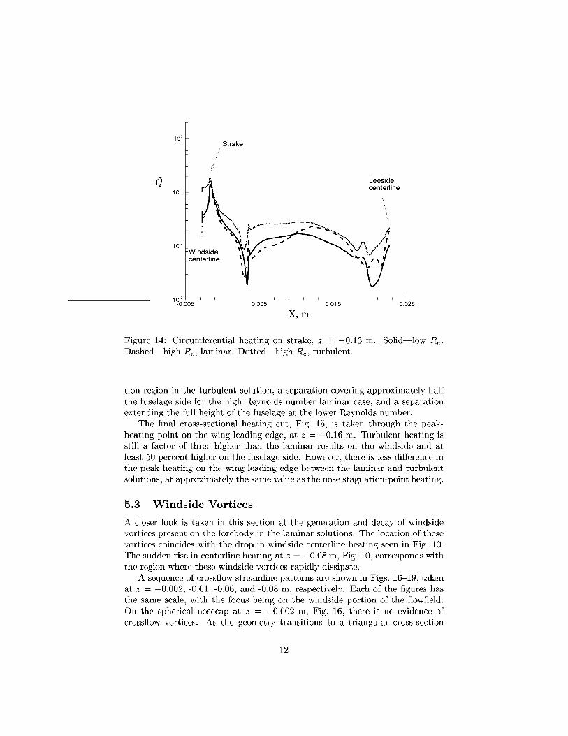
The second cross-sectional heating cut, Fig. 14, is taken on the strake atz -- -0.13 m. This station is where the leeside fuselage transitions from a round
to rectangular profile. Normalized windside heating distributions for the two
laminar solutions are qualitatively similar. The turbulent windside heating is
elevated by a factor of three over the laminar values toward the centerline.
However, the peak normalized heating on the strake leading edge is comparable
for all three cases, at 0 =0.13 0.18. Laminar heating rates on the side of the
fuselage are half the turbulent levels, with the trends suggesting a small separa-

0
10 o
10 _
10 2
Nose
................. °.......................................... , ............................ ..-'°'
Body flap
hinge line
-0.25 -0.2 -0.15 -0.1 -0.05 0
Z;m
Figure 10: Centerline heat transfer rates; windside. Solid low Re. Dashed
high Re; laminar. Dotted high Re, turbulent.
Q
100
10 _
10 2
Vertical tail'o._
"-°°_
4
¢
Nose
°.°° °_
................. ._ .j.._"--.._........ :-
_°. o.*
I I I I I I I I I I I I I I I I I-0.25 -0.2 -0.15 -0.1 -0.05 0
Z; HI
Figure 11: Centerline heat transfer rates; leeside. Solid low Re. Dashed high
Re, laminar. Dotted high Re, turbulent.
10

0
10o
10 _
.."
Wing
,°%°.
y5I
i/.'-0.2
Nose
o°*°°_
Strake ..-'"" ,/.°°°
_ _ _ I _ _ _ _ I _ _ _ _ I _ _ _ _ I-0.15 -0.1 -0.05 0
Z_ Ill
Figure 12: Heat transfer rates along wing leading edge. Solid low Re.
Dashed high Re, laminar. Dotted high Re, turbulent.
0
100
10 _
102
Chine/
Windside Leesidecenterline centerline
1_0;_, _ _ _ _ I _ _ _ _ I _ _ _ _ I.005 0.005 0.015 0.025
X_ m
Figure 13: Circumferential heating on forebody, z = -0.03 m. Solid low Re.
Dashed high R_, laminar. Dotted high Re, turbulent.
11
0
10 o
10 _
102
31
1_00.005
Strake
.-'_ Leeside
._..... _ centerline
'- ;..................................
0.005 0.015 0.025
X, In
Figure 14: Circumferential heating on strake, z = -0.13 m. Solid--low Re.
Dashed high Re, laminar. Dotted high Re, turbulent.
tion region in the turbulent solution, a separation covering approximately half
the fuselage side for the high Reynolds number laminar case, and a separation
extending the full height of the fuselage at the lower Reynolds number.
The final cross-sectional heating cut, Fig. 15, is taken through the peak-
heating point on the wing leading edge, at z = -0.16 m. Turbulent heating is
still a factor of three higher than the laminar results on the windside and at
least 50 percent higher on the fuselage side. However, there is less difference inthe peak heating on the wing leading edge between the laminar and turbulent
solutions, at approximately the same value as the nose stagnation-point heating.
5.3 Windside Vortices
A closer look is taken in this section at the generation and decay of windsidevortices present on the forebody in the laminar solutions. The location of these
vortices coincides with the drop in windside centerline heating seen in Fig. 10.The sudden rise in centerline heating at z = -0.08 m, Fig. 10, corresponds with
the region where these windside vortices rapidly dissipate.
A sequence of crossflow streamline patterns are shown in Figs. 16-19, taken
at z = -0.002, -0.01, -0.06, and -0.08 m, respectively. Each of the figures has
the same scale, with the focus being on the windside portion of the flowfield.
On the spherical nosecap at z = -0.002 m, Fig. 16, there is no evidence of
crossflow vortices. As the geometry transitions to a triangular cross-section
12

100
10 _
102
- Windside
centerline
3 I1O" ' '-0 I O 05
.... _ Wing L.E.
Leesidecenterline
#
, , I , , , , I , , , , I0.005 0.015 0.025
X, nt
Figure 15: Circumferential heating on wing, z = -0.16 m. Solid--low Re.
Dashed high Re, laminar. Dotted high Re, turbulent.
Figure 16: Crossflow streamline patterns at z = -0.002 m.
13
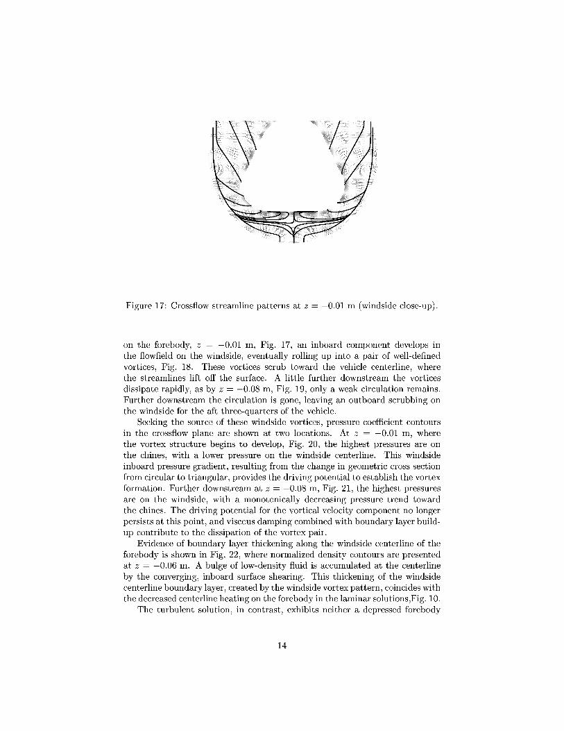
Figure17:Crossflowstreamlinepatternsat z = -0.01 m (windside close-up).
on the forebody, z = -0.01 El, Fig. 17, an inboard component develops in
the flowfield on the windside, eventually rolling up into a pair of well-defined
vortices, Fig. 18. These vortices scrub toward the vehicle centerline, wherethe streamlines lift off the surface. A little further downstream the vortices
dissipate rapidly, as by z = -0.08 m, Fig. 19, only a weak circulation remains.
Further downstream the circulation is gone, leaving an outboard scrubbing on
the windside for the aft three-quarters of the vehicle.
Seeking the source of these windside vortices, pressure coefficient contours
in the crossflow plane are shown at two locations. At z = -0.01 m, where
the vortex structure begins to develop, Fig. 20, the highest pressures are on
the chines, with a lower pressure on the windside centerline. This windside
inboard pressure gradient, resulting from the change in geometric cross section
from circular to triangular, provides the driving potential to establish the vortex
formation. Further downstream at z = -0.08 m, Fig. 21, the highest pressures
are on the windside, with a monotonically decreasing pressure trend toward
the chines. The driving potential for the vortical velocity component no longer
persists at this point, and viscous damping combined with boundary layer build-up contribute to the dissipation of the vortex pair.
Evidence of boundary layer thickening along the windside centerline of the
forebody is shown in Fig. 22, where normalized density contours are presentedat z = -0.06 El. A bulge of low-density fluid is accumulated at the centerline
by the converging, inboard surface shearing. This thickening of the windside
centerline boundary layer, created by the windside vortex pattern, coincides with
the decreased centerline heating on the forebody in the laminar solutions,Fig. 10.
The turbulent solution, in contrast, exhibits neither a depressed forebody
14
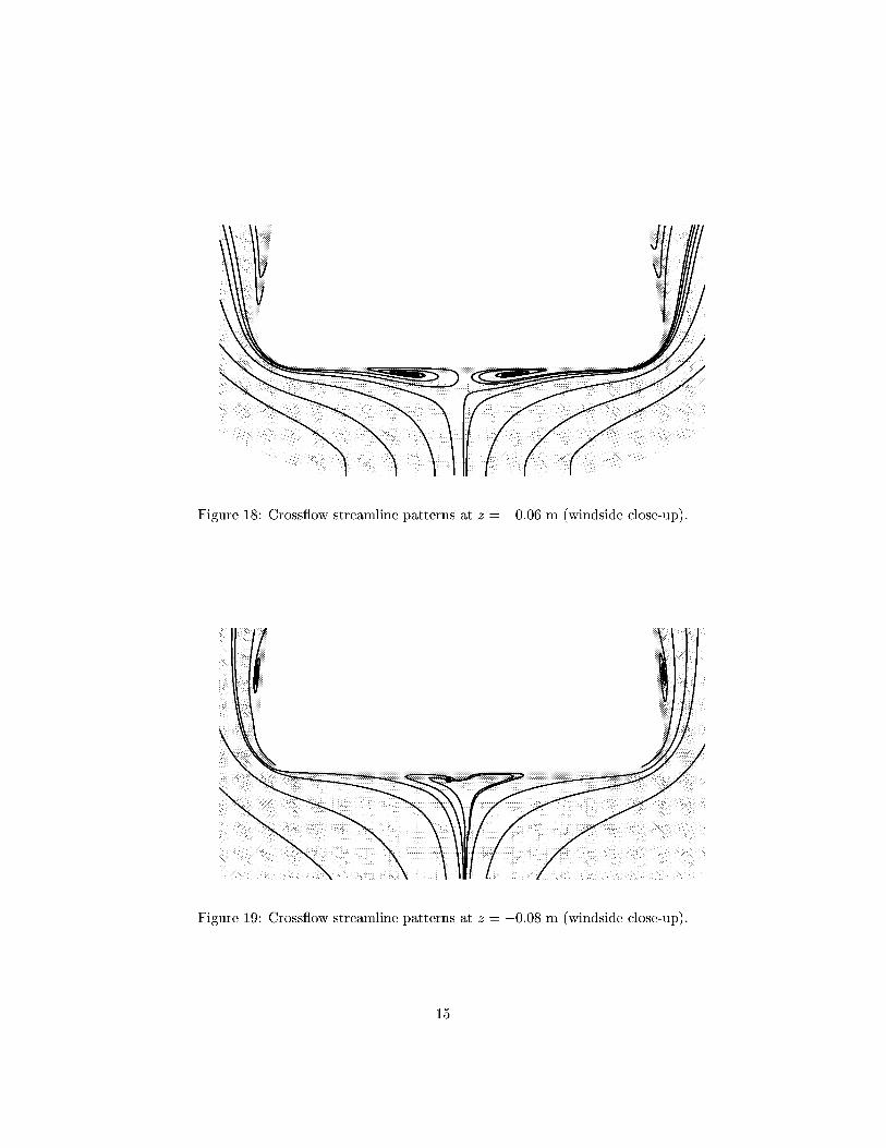
Figure18:Crossflowstreamlinepatternsat z = -0.06 m (windside close-up).
ii
/
Figure 19: Crossflow streamline patterns at z = -0.08 m (windside close-up).
15

Op
0.25
0.20.150.1
0.050
Figure 20: Pressure coefficient in the cross-flow plane at z = -0.01 m (windside
close-up).
Cp0 0.05 0.1 0.15 0.2 0.25
Figure 21: Pressure coefl]cient in the cross-flow plane at z = -0.08 m (windside
close-up).
16

Figure22:Densitycontoursin thecross-flowplaneat z -- -0.06 m (windside
close-up).
centerline heating nor windside vortices on the forebody. The much greater
effective boundary layer viscosities for the turbulent case may inhibit the for-mation of these structures.
6 Summary of Results
A computational study has been performed for the X-34 vehicle (truncated at
the body-flap hinge line) at Mach 6 wind tunnel conditions. Two Reynolds
numbers are considered, with both laminar and turbulent solutions obtained at
the higher Reynolds number.
The effects of Reynolds number variation and turbulence on normalized
surface heat-transfer rates are compared using both surface contour plots and
extracted-data line plots. Reynolds number variation on laminar solutions has
little effect on the normalized windside heating. Some variation in leeside center-
line heating is seen between the laminar solutions at different Reynolds numbers.
The increase in heating due to turbulence is seen to vary with location on the
vehicle. General trends show windside turbulent heating to be as much as four
times greater than laminar heating. On the leeside, the effect of turbulence is
most pronounced on the forebody, where heating is elevated by a factor of two.Wing leading edge heating, which is comparable in magnitude to the stagnation
point heating, is less effected by turbulence, showing a 30 percent rise over thelaminar values.
An abrupt increase in windside centerline heating is indicated for the lain-
inar cases at one-quarter of the vehicle length, unexpected because of the flat,
17
featurelessbottomonthevehicleat that point.Furtherinvestigationrevealsapairofwindsidevorticesupstreamoftheheatingrise,generatedbythenosecap-to-forebodychangein crosssectionon thevehicle.Thesevorticesdissipateatexactlythesamelocationastheheatingincrease.Thepostulationis thatthesevorticesaccumulateathickerwindsideboundarylayeralongthecenterlineoverthequarterforebodyofthevehicle,locallydepressingthecenterlineheating.Asthesevorticesdissipate,thecenterlineheatingrisesto thegeneralvalueoverthewholeoftheflatwindsidefuselage.Neitherthewindsidevorticesnoraheatingchangeat thequarterforebodylocationareobservedin theturbulentresults.
References
[1] Foley, T. M., "Big Hopes for Small Launchers," Aerospace America, Vol. 33,No. 7, Jul. 1995, pp. 28 34.
[2] Cook, S. A., "The Reusable Launch "Vehicle Technology Program and the
X-33 Advanced Technology Demonstrator," NASA TM 111868, Apr. 1995.
[3] NASA, "Reusable Launch Vehicle (RLV), Small Reusable Booster, X-34,"
Cooperative Agreement Notice CAN 8-2, Jan. 1995.
[4] Kleb, W., Wood, W., Gnoffo, P., and Alter, S. J., "Computational Aero-
heating Predictions for X-34," AIAA Paper 98 0879, Jan. 1998.
[5] Berry, S., Horvath, T., DiFulvio, M., Glass, C., and Merski, N. R., "X-34
Experimental Aeroheating at Mach 6 and i0," AIAA Paper 98-0881, Jan.1998.
[6] Merski, N., "Reduction and Analysis of Phosphor Thermography Data withthe IHEAT Software Package," AIAA Paper 98 0712, Jan. 1998.
[7] Kleb, W. L., Wood, W. A., and Gnoffo, P. A., "Computational Aeroheating
Predictions for X-34," NASA/TM 1998 206289, USA, Jan. 1998.
[8] Riley, C., Kleb, W., and Alter, S. J., "Aeroheating Predictions for X-34
using an Inviscid-Boundary Layer Method," AIAA Paper 98-0880, Jan.1998.
[9] Alter, S. J., "Surface Modeling and Grid Generation of Orbital Science's
X-34 Vehicle (Phase I)," Contractor Report CR97 206243, NASA, Nov.1997.
[I0] Cheatwood, F. M. and Gnoffo, P. A., "User's Manual for the Langley
Aerothermodynamic Upwind Relaxation Algorithm (LAURA)," NASA TM
4674, Apr. 1996.
[11] Gnoffo, P. A., Gupta, R. N., and Shinn, J. L., "Conservation Equations
and Physical Models for Hypersonic Air Flows in Thermal and Chemical
Nonequilibrium," NASA TP 2867, Feb. 1989.
18

[12]Gnoffo,P.A., "An Upwind-Biased,Point-ImplicitRelaxationAlgorithmfor Viscous,CompressiblePerfect-GasFlows,"NASATP 2953,February1990.
[13]Navier,M., "M_moiresurlesloisduMouvementdesFluides,"Mdmoire de
l'Acadgmie des Sciences, Vol. 6, 1827, pp. 389.
[14] Stokes, G. G., "On the Theories of the Internal Friction of Fluids in Mo-
tion," Trans. Cambridge Philosophical Society, Vol. 8, 1849, pp. 227-319.
[15] Baldwin, B. S. and Lomax, H., "Thin Layer Approximation and Algebraic
Model for Separated Turbulent Flows," AIAA Paper 78 257, January 1978.
[16] Cheatwood, F. M. and Thompson, R. A., "The Addition of Algebraic Tur-
bulence Modeling to Program LAURA," NASA TM 107758, April 1993.
[17] Gnoffo, P. A., Weilmuenster, K. J., Hamilton, H. H., Olynick, D. R., andVenkatapathy, E., "Computational Aerothermodynamic Design Issues for
Hypersonic Vehicles," AIAA Paper 97-2473, Jun. 1997.
[18] Weilmuenster, K. J., Gnoffo, P. A., Greene, F. A., Riley, C. J., Hamilton,H. H., and Alter, S. J., "Hypersonic Aerodynamic Characteristics of a Pro-
posed Single-Stage-to-Orbit Vehicle," Journal of Spacecraft and Rockets,
Vol. 33, No. 4, Jul. 1996, pp. 463 469.
[19] Weilmuenster, K. J., Gnoffo, P. A., and Greene, F. A., "Navier-Stokes Sim-
ulations of the Shuttle Orbiter Aerodynamic Characteristics with Emphasis
on Pitch Trim and Body Flap," AIAA Paper 93-2814, July 1993.
[20] Fay, J. A. andin Dissociated
Feb. 1958, pp.
Riddell, F. R., "Theory of Stagnation Point Heat Transfer
Air," Journal of the Aeronautical Sciences, Vol. 25, No. 2,73 85.
[21] Brauckmann, G. J., "X-34 Vehicle Aerodynamic Characteristics," AIAA
Paper 98 2531, Jun. 1998.
19
REPORT DOCUMENTATION PAGE FormApprovedOMB No. 0704-0188
Public reporting burden for this collection of information isestimated to average 1 hour per response, includingthe time for reviewing instructions, searching existingdata sources,gathering and maintainingthe data needed, and completing and reviewingthe collection of information. Send comments regarding this burden estimate or any other aspect of thiscollection of information, including suggestions for reducing this burden, to Washington HeadquartersServices, Directoratefor Information Operationsand Reports, 1215 Jefferson DavisHighway, Suite 1204, Arlington, VA 22202-4302, and to the Office of Management and Budget, Paperwork Reduction Project (0704-0188), Washington, DC 20503.
1. AGENCY USE ONLY (Leave blank) 2. REPORT DATE 3. REPORT TYPE AND DATES COVERED
February 1999 Technical Memorandum
4. TITLE AND SUBTITLE
Aerothermodynamic Calculations on X-34 at Mach 6 Wind TunnelConditions
6. AUTHOR(S)
William A. Wood
7. PERFORMING ORGANIZATION NAME(S) AND ADDRESS(ES)
NASA Langley Research CenterHampton, VA 23681-2199
9. SPONSORING/MONITORING AGENCY NAME(S) AND ADDRESS(ES)
National Aeronautics and Space AdministrationWashington, DC 20546-0001
5. FUNDING NUMBERS
WU 242-80-01-01
8. PERFORMING ORGANIZATIONREPORT NUMBER
L-17794
10. SPONSORING/MONITORINGAGENCY REPORT NUMBER
NASA/TM-1999-208998
11. SUPPLEMENTARY NOTES
12a. DISTRIBUTION/AVAILABILITY STATEMENT
Unclassified-UnlimitedSubject Category 16,34 Distribution: StandardAvailability: NASA CASI (301) 621-0390
12b. DISTRIBUTION CODE
13. ABSTRACT (Maximum 200 words)
The effects of Reynolds number and turbulence on surface heat-transfer rates are numerically investigated for a0.015 scale X-34 vehicle at wind tunnel conditions. Laminar heating rates, non-dimensionalized by Fay-Riddellstagnation heating, do not change appreciably with an order of magnitude variation in Reynolds number. Modelinga turbulent versus laminar boundary layer at the same Reynolds number increases the windside heating by a factorof four, portions on the leeside by a factor of two, and causes a 30 percent increase in wing leading edge heating. Adiscrepancy between laminar and turbulent heating trends on the windside centerline is explained by the presenceof attached windside vortices in the laminar solutions, structures that are inhibited by the turbulence modeling.
14. SUBJECT TERMS
X-34, access to space
17. SECU RITY CLASSIFICATIONOF REPORT
Unclassified
18. SECURITY CLASSIFICATIONOF THIS PAGE
Unclassified
19. SECU RITY C LASSIFICATIONOF ABSTRACT
Unclassified
15. NUMBER OF PAGES
24
16. PRICE CODE
A03
20. LIMITATION OF ABSTRACT
NSN 7540-01-280-5500 Standard Form 298 (Rev. 2-89)PrescribedbyANSI Std. Z39-18298-102