Aerospace research through statistical engineering · Aerospace research through statistical...

Calhoun: The NPS Institutional Archive

Faculty and Researcher Publications Faculty and Researcher Publications Collection

2012

Aerospace research through statistical engineering

Silvestrini, Rachel T.

Taylor & Francis

Quality Engineering, v.24, 2012, pp. 292-305

http://hdl.handle.net/10945/47555

Aerospace Research throughStatistical Engineering

Rachel T. Silvestrini1,Peter A. Parker2

1Operations ResearchDepartment, Naval PostgraduateSchool, Monterey, California2National Aeronautics and SpaceAdministration, Hampton,Virginia

ABSTRACT The application of statistical engineering as described here is

applied to fundamental research in support of hypersonic air breathing

propulsion. An aerospace experiment that took place in a wind tunnel is

the application of interest. One goal of the project was to accurately model

the relationship between specific input and output parameters in the hyper-

sonic combustion process within a controlled environment. Response surface

methodology (RSM) was applied in a nontraditional manner to develop the

response surface as the final deliverable rather than a tool to optimize a

product or process.

KEYWORDS design of experiments, face-centered cube, repeat measures,

replication, sample size

INTRODUCTION

This article presents the successful implementation of statistical engineer-ing applied to aerodynamic research at NASA’s Langley Research Center.The implementation of the statistical methodology was described in detailin a paper published by Johnson et al. (2009). In this article, we will revisitthe supersonic combustion experiment but discuss the experiment to high-light the entire statistical engineering process rather than an emphasis on thestatistical tools and methods.

Statistical engineering as described here is applied to fundamentalresearch in support of hypersonic air breathing propulsion. The probleminvolved a high degree of complexity to accurately model the relationshipbetween specific input and output parameters in the hypersonic combustionprocess within a controlled environment. The experiment was designed tocharacterize flow-field parameters as a function of the location, specificallyaxial and radial distance, within a coaxial free jet. The characterizationexperiment required the adaption and extension of response surfacemethodology (RSM) to study turbulent mixing properties with the goal toimprove computational modeling.

The flow-field responses are unsteady (turbulent) due to instabilities;however, the experiment is designed such that the distribution of the flowparameters, mean and variance, are statistically stationary. Ultimately theresearchers are interested in understanding the effect of turbulence through

This article is not subject to U.S.copyright law.

Address correspondence to Peter A.Parker, NASA Langley ResearchCenter, MS 238, Hampton, VA 23681,USA. E-mail: [email protected]

Quality Engineering, 24:292–305, 2012ISSN: 0898-2112 print=1532-4222 onlineDOI: 10.1080/08982112.2012.641146

292

a collection of statistics such as mean, variance, andcovariance of parameters of interest throughout theentire jet engine flow field.

In this application, a statistical engineeringapproach was able to deliver an experimentalapproach to meet the specified objectives, and itclearly managed expectations about what could beobtained within the severe resource constraints priorto execution. As a result of this particular study andnumerous other examples, the use of a statisticalengineering approach is now becoming more widelyaccepted for these types of experiments. The impactis more efficient aerospace research that enables ourknowledge to increase more quickly.

This article provides a case study of applying a stat-istical engineering approach to common class ofproblems encountered in aerospace research. Weseek to highlight the application of statistical engin-eering and, in particular, the collaborative effort toestablish a systematic method for solving complexproblems of this nature. Moreover, we highlightefforts that NASA has made to improve the collabor-ation between statisticians and engineers=physicists.Aerospace research is a process of discovery, requir-ing a series of experiments that require efficientexperimental design techniques. These techniquesalso often require the blending of many differentstatistical toolsets, combined with nonstatisticalknowledge to fit the complexity and restrictions ofthe problem at hand. This article represents a success-ful illustration of the strategy for blending differentstatistical tools sets along with subject matter expert-ise that is applicable to many aerospace researchprojects.

BACKGROUND

Ground-based laboratory research facilities areused to simulate flight conditions to support a widevariety of aerospace research. In particular, recentresearch efforts include the study of supersonic andhypersonic flight and propulsion. Understandingthe aerodynamic properties of supersonic and hyper-sonic flight is extremely important to the success ofnew aircraft that achieve speeds required by theseflights. Barnstorff (2007) stated that these experi-ments help NASA engineers ‘‘address some of thechallenges of hypersonic flight, a speed regime that’sdifficult to simulate and predict’’ (p. 11).

Experimentation in these types of facilities iscomplex and expensive. For these two reasons, it isimportant to develop statistically sound methodsfor developing and carrying out experiments that willbe conducted in order to maximize the knowledgeobtained. Developing statistically sound methodsis a process that involves multiple subject-matterexperts (SMEs) across multiple science and engineer-ing disciplines. In the next section we introduce thestatistical engineering approach that integratedcomputational fluid dynamics (CFD) modelingresults, SME input, and several experimental designapproaches to developing an overall experimentaldesign strategy for a hypersonic wind tunnel test.An application of this methodology will then beillustrated, followed by a discussion.

METHODOLOGY

Statistical engineering is the terminology thatdescribes the overall approach we used to developa methodology that can be used to integrate CFDresults and SME knowledge into experimental deci-sions as shown in Figure 1. As mentioned in theBackground section, this problem is not unique tothe application discussed in the next section; it is areoccurring problem that could greatly benefit froma standardized approach.

Montgomery (2009) described statistical design ofexperiments as the ‘‘process of planning the experi-ment so that appropriate data will be collected andanalyzed by statistical methods, resulting in validand objective conclusions.’’ This process includes asequence of steps that start with preexperimentalplanning and end with conclusions and recommen-dations. For a detailed discussion on the process ofdesigning and analyzing experiments, see Colemanand Montgomery (1993). Simpson et al. (2011)

FIGURE 1 External influences used for the development of theexperimental design used for testing. (Color figure availableonline.)

293 Aerospace Research through Statistical Engineering

discussed the design of experiments (DOE) processas a circular cycle of experimentation. The steps inthe circular experimentation process are summarizedinto four broad categories: plan, design, execute, andanalyze. Figure 2 illustrates these steps and highlightsthe area of discussion, planning, and designing in thisarticle. The integration of CFD model results and SMEknowledge into an aerospace test requires an exten-sive iterative process in the planning and designingphase of experimental design and analysis. Thoughthe focus of this article is on the plan and designsteps, we will also briefly discuss the execute andanalyze steps of the process through an applicationusing a portion of CFD results.

Experimental designs are created in order to meetthe goals of the problem as it is defined. The choice ofdesign is based on a goal that typically falls into oneof three categories: screening design, response sur-face methodology, or robust process design. Resultsfrom aerospace experiments are often utilized bymany groups of people involved in the researchprocess. Because of this, experiments often have avariety of goals that span multiple categories. Com-mon statistical research tools and=or considerationsthat aerospace experiments and data analysis relyon include but are not limited to the following:

. Response surface methodology

. Robust process design (RPD)

. Complex statistical inference

. Data analysis for multiple responses

. Repeat measures

. Limitations of experiments due to physics constraintsand=or equipment constraints

The theoretical foundation surrounding the tools andmethods was used to create an integrated approach

to wind tunnel experiments. The strategy used tointegrate the tools was based on combining standardexperimental design process in combination withSME involvement. Based on the needs of the projectand the requests for information, it becameevident that these tools were required throughoutthe process.

The first part of the experimental design processincludes the planning phase as shown in Figure 2.In the methodology we suggest, we use the samepreexperimental phases as given in Montgomery(2009), which include recognition of the statementof the problem, selection of the response variables,and choice of factors, levels, and ranges. In ourexperience, no aerodynamic experiment is focusedon a single response variable, so we would like toemphasize the selection of multiple response vari-ables. In this phase of the experimental planning, itis extremely important to have group meetings withall of the SMEs involved. This includes but is notlimited to the physicists, statisticians, and engineersinvolved in both computational experiments andlaboratory experiments.

The second part of the experimental design pro-cess covers the choice of experimental design. Wehave expanded this phase to include additional com-ponents beyond the goals of the experiment (whichare identified in the planning phases under recog-nition and statement of the problem). The initialexperimental design is modified by the use CFDresults and modifications required by the physicsand engineering concerns as depicted in Figure 3.

The overall process of planning and designing theexperiment is presented in Figure 3. In the Application

FIGURE 2 Experimental design focus; the iterative processbetween the planning and designing phases in experimentaldesign. (Color figure available online.)

FIGURE 3 Planning and designing phases of aerospace exper-imentation. (Color figure available online.)

R. T. Silvestrini and P. A. Parker 294

section, we identify the specific areas of research; forexample, statistical inference, response surface meth-odology, and engineeringmodifications that influencethe final choice of design.

AN APPLICATION OF AEROSPACEEXPERIMENTATION

This section is divided into three subsections:Planning (planning of the laboratory experiment),Designing (designing the experiment), and Execut-ing and Analyzing (illustrating modeling approachesusing CFD test data). An important facet of statisticalengineering is that there is considerably more effortrequired to assist the SME to unequivocally definethe objectives. In this example, we emphasize thesolicitation and interpretation from the SME toensure that we are solving the right problem.

Planning

Planning an experiment, as shown in Figure 3,includes all of the preexperimental design phasesof the experimental design and analysis process.There are three main components to this phase: rec-ognition of the statement of the problem, selection ofthe response variables, and choice of factors, levels,and ranges.

Recognition of the Statement ofthe Problem

The experimental design was created to ultimatelycharacterize a number of flow-field parameters(response) as a function of the location within acoaxial free jet. From a physics and engineering per-spective, this would allow the study and advancedresearch in turbulent mixing and computational mod-eling (for use in developing and validating the CFD).Ultimately the researchers involved in the project areinterested in understanding the effect of turbulencethrough a collection of statistics. Essentially, the goalswere to provide a comprehensive set of descriptiveand inferential statistics and to characterize theresponse surface through the use of several differentmathematical models.

At first glance, this goal seems to be RSM. How-ever, the inferential statistics, complexity of the differ-ent responses, and the need to integrate CFD with theapproach pulled this application out of the realm of

RSM. This application involved a high degree ofcomplexity, requiring more than one statistical tech-nique to solve, and required both technical and non-technical challenges, such as communication across anumber of SMEs.

Choice of Response Variables

There are six main response variables of interest,shown in Table 1. In addition to these six responsevariables, it was of interest to characterize not onlythe mean of each response as a function of the inputfactors but also the variance and the covarianceamong pairs of responses. In addition to the sixmean responses, there are six variance measure-ments (one for each response) and 15 (six choosetwo) covariance measurements. This makes a totalof 27 responses of interest.

Choice of Factors, Levels, and Ranges

There are only two inputs of interest in the experi-ment, which are located within the open jet flame.The open jet flame is a three-dimensional area, butonly two dimensions are modeled for the purposeof this experiment. An infrared image of the flamewithin an open jet can be seen in Figure 4, along witha picture of a cross section along the axis of the jetengine nozzle. (Note that the picture is compressedby a factor of 2 along the x-axis relative to the r-axisfor the purpose of illustration.) Figure 4 also illus-trates, for reference, the two input factors (x-axisand r-axis, both measured in millimeters) and theirdirectionality within the open jet flame. It wasassumed that the response would be symmetric aboutthe z-axis (third dimension, going into the page), thusremoving the need for a third input factor.

Designing

Developing an experimental design based on theunique goals and the complexity of aerodynamic

TABLE 1 Responses of interest in the wind tunnel tests

Temperature (K)u-Axis velocity (m=s)v-Axis velocity (m=s)N2 (%)H2 (%)O2 (%)


research is considered a phase in itself. We treat thecreation of the experimental design as a process thatinvolves all of the SMEs interested in the problem.Though this phase is iterative, we discuss each ofthe four main components separately in this article.The components, as shown in Figure 3, are selectionof the experimental design based on the statement ofthe problem (and goals of the experiment), use of theCFD results to modify experimental design choice,physicist SMEs’ input=modification of the design,and engineers’ input=modification of the design.

Note that using an experimental design approachfor this problem is actually a unique application ofexperimental design in itself. This is because weusually think of experimental design as a way of con-trolling factors and studying their relationship (if any)with respect to a response. Our factors in this studyare locations within an open jet flame. Thus, we areusing experimental design as a sampling strategy.

Choice of Experimental Design

Employing design of experiments principles inhypersonic research has greatly improved the cost-effectiveness and information efficiency comparedto previous methods. The choice of experimentaldesign should always support the goals of the pro-ject and experiment. In the case of this application,the goals were quite broad and somewhat vague.There were so many SMEs involved in the experi-ments that a concise description incorporating allstakeholders’ goals was challenging. As mentionedin the section ‘‘Recognition of the Statement of theProblem,’’ the goals of the experimentation wereto provide a comprehensive set of descriptive and

inferential statistics and to characterize the responsesurface through the use of several different math-ematical models.

The present experiment was an extension from asmall-scale study to full-scale apparatus and was partof a much larger research effort in hypersonic air-breathing propulsion. As a result of this, there wasprior knowledge available about several portions ofthe expected results. Prior knowledge about expectedoutcome of experiments can greatly aid the experi-mental design process. In particular, the prior knowl-edge provided the general nature of several of theresponse surfaces. This prior knowledge led to theestablishment of several assumptions:. Axis symmetric flow field. Less drastic change in the x-axis direction than ther-axis direction

. Sharp points of inflection in the design space at theshear layer (see Figure 5)

. Constant gas flow rate during testing

. Unsteady flow-field parameters

The use of these assumptions allowed the experi-mental design to be developed in a more efficientmanner. The axis symmetry assumption led to theremoval of the rotational axis (as mentioned in the‘‘Choice of Factors, Levels, and Ranges’’ section),meaning that the design was two-dimensional asopposed to three. The less drastic change in the x-axis direction than in the r-axis direction allowedfor wider spacing of design points in the x-axis

FIGURE 5 Angled–nested FCCD design based on peak anglewith respect to the open jet nozzle.

FIGURE 4 Diagram of the Mach 1.6 nozzle and infrared imageof the open jet that issue from the nozzle.


direction and more densely packed points in ther-axis direction. Additional points at the shear layerlocation were found to be very important due to thesharp transitions of response variable outputs andthe need for higher fidelity models around the shearlayer. The flow-field parameters are expected to beunsteady (turbulent) due to instabilities; however,the experiment is designed such that the distributionof the flow parameters, mean and variance, are stat-istically stationary.

The data collected from the experiment will beused for the development of response surface mod-els over different, sometimes overlapping, regionsin the design space. Therefore, the precise estimationof single points of data, the ability to fit varying typesof models, and the ability to fit models of both meanand variance were all of equal importance. Finally,the focus on the precision of the response surfacefor both mean and variance models of a particularvariable was of interest. Modeling the relationshipof the variance of a response variable for multiplerandom variables is not a topic that is often discussedor found in the literature. Vining and Schaub (1996)discussed designs for mean and variance functionsof variables. Other useful references on this topiccan be found in Myers et al. (2009). This statisticalengineering application illustrates the use of a modi-fied, partitioned classical experimental design in aninnovative manner that accounts for the unusualdesign problem, design restrictions, and incorporatesa robust method of systematically accounting fornoise, or variability of the responses, inherent inthe system.

In this case, RSM was applied in a nontraditionalmanner to develop the response surface as the finaldeliverable rather than a tool to optimize a productor process. In classical RSM, the goal is to approxi-mate the response surface in order to specify optimalfactor settings; in this usage of RSM we are not seek-ing to optimize the location within the flow field butrather to efficiently characterize the flow field todevelop insights and to compare the experimentalresults with computational prediction. Though thismay seem to be a relatively minor difference in ourgoal, it has a significant impact on the design. Forexample, we are interested in specifying a designthat produces an absolute prediction variance, ratherthan a design with certain efficiency that essentiallyconsiders the reduction in prediction variance per

point. In this case, we are interested in the unscaledprediction variance.

Another departure from classical RSM is our desireto develop a global response surface over the entireregion of interest, or a partitioned quilt of responsesurfaces rather than a confirmed response surface ina local region of estimate optimum conditions, whichis the classical RSM objective. Due to the complex andpotentially discontinuous nature of the entire regionof interest, the design region was partitioned toprovide local second-order response surfaces in sub-regions of interest. This design approach also sup-ports higher-order models over larger subregionsand nonparametric modeling approaches.

Discussions about potential outcomes of theresponse variables, what types of models would beof interest to fit, and the design region lead to severaloptions in the choice of experimental design thatcould be used. The following design types wereconsidered:. Optimal designs (D and I). Classical designs. Space filling designs

Design D- and I-optimality were omitted as poten-tial options early in the experimental design discus-sions due to uncertainty regarding the model overthe entire space and the need to fit multiple models,perhaps in a piecewise manner, across the designregion. Montgomery (2009) pointed out that optimaldesign criterion are of particular interest when theform of the model is known prior to experimen-tation. In this case, small-scale experimentationdemonstrated very complex nonlinear models overlarge regions of the design space. Speculations aboutmodel forms over very small regions of the designspace led to the possibility of piecewise second-order models.

The choice of a classical design often used inresponse surface methodology (Myers et al. 2009) isusually the central composite design (CCD). TheCCD has the ability to fit up to a second-order modeland consists of only nine design points in two factors.In two factors, the design has four corner runs, fouraxial runs, and a center run. In a spherical designspace, the axial runs are set on the outside of thesquare region, so that the points lie along a circlesurrounding the center point. Due to the near-rectangular design space, a face-centered central


composite design (FCCD; also known as the facecentered cube—FCC) was chosen over the CCD. Inthis design, the axial runs lie on the edge centers ofa cuboidal space.

Space-filling designs are experimental designs thataim to fill the interior of a design region. The lowerand upper bounds on the input variables definethe design region. For a comprehensive discussionabout different space filling designs see Santneret al. (2003) or Fang et al. (2006); also see Jonesand Johnson (2009) for a graphical example of fivedifferent space-filling designs placed in a two-dimensional input design region.

The choice of space-filling designs is compellingfor use in deterministic computer simulation models,where the output response does not have a stochasticcomponent. The classical design option for responsesurface modeling was placed above the space-fillingoption because of the highly stochastic nature ofthe response variable, the experimenters’ previousexperience, and the need to fit models along radialtraces (see x-axis locations; see Figure 4). Also, indesigns such as the FCCD, near uniformity is attained,making it an attractive choice, especially if the needfor a nonparametric model is foreseen.

Use of CFD to Modify Experimental Design

The FCCD design was chosen as the initial experi-mental design choice. The FCCD was chosen for sev-eral reasons, including the fitting of second-ordermodels and its near uniformity. We mean that theFCCD has points spread equally throughout the regionof design space, and this property is ideal for the fittingof both parametric and nonparametric models. TheFCCD, though an excellent choice for RSM problems,was expected to have several drawbacks. The first setsof modifications to the design were created based onboth infrared pictures of the small-scale open jetexperiment and the CFD output results. The CFDmodel was a simulation model developed to mimicreal aerodynamic properties of hypersonic flight.

Though a traditional FCCD (classical squareshape) was used to start with, it was determined thatthe design needed to be set at an angle to the nozzleexit of the jet so that each of the points was on linesof a particular slope as opposed to parallel lines onthe horizontal. This created a truncated cone shapeinstead of the traditional square. The reason for this

modification of the classic design was due to theshape of the design region and the knowledge ofthe turbulent flow patterns throughout the open jetflame. The FCCD was set at angles correspondingto patterned turbulent flows exiting the nozzle head.See Figure 5 for the truncated cone shaped designregion. Figure 5 also illustrates where the shear layeris located. From an experimental design perspective,the design region is a truncated cone shape withfurther restricted regions due to the data collectionapparatus and its mobility limitations. In essence, thisdesign approach mapped a nonrectangular truncatedcone shape into a coded rectangular region where aFCCD was specified.

In addition to the modified shape of the FCCD, itwas determined that a single FCCD would not pro-vide enough degrees of freedom to fit the complexresponse expected in the r-axis direction because ofthe need for a much higher fidelity model over thelarger design regions. In addition, the ability to poss-ibly fit piecewise polynomial models in smallerdesign regions was desired. Therefore, it was decidedthat stacked FCCD designs would be implemented.Note that we could have chosen a single design withmore levels (for example, a factorial with nine levelsin each factor), which essentially would result in thesame design we created. But because we wanted tovisualize the piecewise polynomial models, so wechose to design and think about the factor space interms of layered FCCDs.

Three FCCD design were stacked on top of theother with overlapping top and bottom points.Figure 5 illustrates three stacked FCCDs, whichresults in seven design points along each of threeradial traces (r-axis lines at a given x-axis location).If the FCCDs were not overlapped, three FCCDdesign would create nine points along each of thethree the radial traces; therefore, a saving of sixdesign points was realized. Therefore, a stackedFCCD approach was used to fill the design space.In essence, the design consisted of a stacked andnested FCCD, which provides the largest preexperi-mental flexibility for modeling options over largersubregions or employing higher-order models. Incontrast to a purely space-filling design, we incor-porated all of the SME prior knowledge based oncomputational simulation and previous small-scaleexperiments to efficiently sample the entire regionof interest.


The modified FCCD was attractive for two reasons:not only did it meet the ability to match patterns ofthe turbulent flow but it was also consistent withthe shape of the flame that results after the combus-tion takes place.

The region of experimentation spanned a large dis-tance in the x-axis direction (relative to the r-axisdirection). Three FCCD designs as shown in Figure 5were only enough to capture a small part of thedesign region just after the nozzle exit. One of theinitial modeling assumptions listed was that therewould be less drastic changes in the flow-field para-meters, or response variables, in the x-axis direction.This assumption paired with the design space led tothree main design regions of interest. The stackedFCCDs were therefore repeated in three separatedesign regions. The edges of each design region wereoverlapped so that savings on design point locationscould be realized. A single region contained 21design points, seen in Figure 5, so three regionswould have a total of 63 design points, but becauseof the overlapping among the three regions of nestedFCCDs only 49 design points were needed to coverthe full region of interest. The adaptive scaling ofthe designs along the factor space based on priorknowledge dramatically reduced the number ofdesign points while maintaining the ability to capturethe behavior of the flow field.

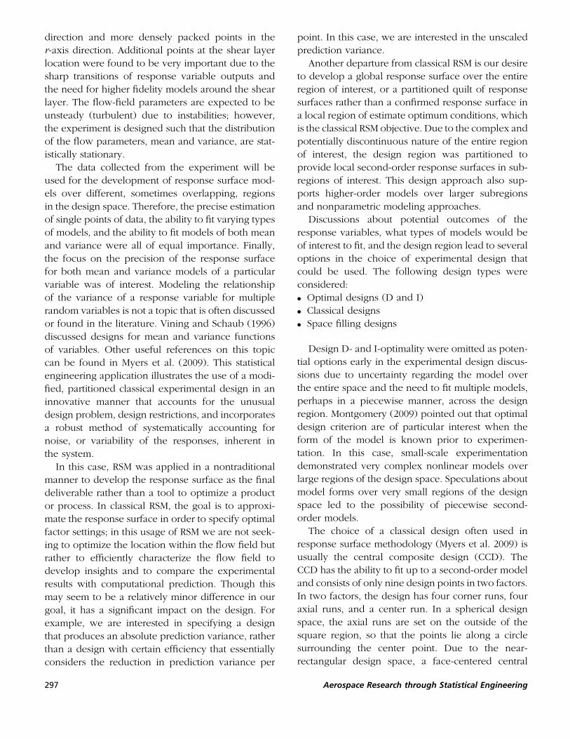
Another modeling assumption mentioned was thesharp inflection points in the response variables inthe radial axis direction due to steep gradients ofvariability in turbulent flow. At these points, evenhigher fidelity models were required. In the openjet experiment, nonconstant variance was expected,but no models of its form were known prior to exper-imentation. Only the knowledge that there would bean increase in turbulence, translating to extra varia-bility, along the line known as the shear was avail-able. The need for more points in regions of highervariance, without the knowledge of the form of thevariance structure, led to the addition of points alongseveral radial traces (or fixed x-axis locations inpoints of high gradient areas as seen from previousCFD models). Figure 6 shows several of the x-axisdesign locations with added radial (r-axis) points inregions of high gradient. Ultimately, the choice wasmade to add nine extra design points in the firstregion of the design space. This resulted in the modi-fied FCCD design containing 58 unique locations.

Physicists’ Concerns and the Modificationof the Experimental Design

Several of the SMEs involved in the wind tunnelexperiments were interested in purely descriptiveand inferential statistical measures of the responses.Of particular interest was the variability over time ata single location under homogenous experimentalconditions. In order to achieve precise statisticalmetrics concerning the mean and variance of theresponses, it was important to control the subsampleswithin a single design point. The idea of subsamplingis different than replication in that the subsamples arerepeat measurements taken by the measurementapparatus at a specific location prescribed by thedesign. Note that replications, which are visits backto that same design point location, are also important,especially in terms of the mathematical model. Repli-cation is addressed in the next section on engineers’concerns.

In this section, we illustrate the development ofthe subsampling strategy by first introducing somebasic statistical notation and then developing themethod used in the experiment with a more sophis-ticated example and sensitivity analysis.

Let yi be a single measurement at one location inthe flow field, which we assume to be independentand identically distributed (iid) normal with a meanof ly and a variance r2y. Let multiple measurementsat a single location be denoted by a vector

y ¼ y1; y2; . . . ; ys½ #0

where s is the number of measurements at a designpoint. We refer to these readings as subsamples

FIGURE 6 Illustration of CFD results with added points inregions of high gradient.


because multiple measurements at a single designpoint, without changing x-axis or r-axis (the inputs),are not replicate measurements but rather repeatmeasurements.

There are two main components that contribute tothe variability among the measurements in y. Theyare the measurement system noise (also referred toas precision of the measurement system), r2m, andthe variability in the flow media (turbulent flow),denoted by r2t . Therefore, we can write

r2y ¼ r2m þ r2t ½1#

Note that we cannot separate the measurementsystem noise from the turbulence in a single experi-ment. Therefore, an estimate of r2m was obtained ina nonturbulent flow field. The estimation of r2t isintuitively restricted by r2m. Using this notation, wecan illustrate the estimate of the mean and varianceof the response the vector y as, m̂my ¼ !yy and r̂r2y ¼ S2,respectively. These statistics are both unbiasedestimators and their variances are

Var l̂ly! "

¼r2ys

½2#

Var r̂r2y! "

¼2 r2y! "2

s% 1¼

2r4ys% 1

½3#

We see that increasing the number of measurements,s, at a single design point decreases the variance of mylinearly and the standard deviation by

ffiffis

p. However,

the variance of r̂r2y is a power of 2 larger than that ofmy. Clearly, this implies the estimation of a variancerequires more subsamples, a well-known result.See Casella and Berger (2002) for a discussion ofEq. [3].

Though Eqs. [2] and [3] describe the variance offlow-field parameters at a single design pointlocation, we are also interested in identifying andquantifying the sources of variability over the entireflow field. To do this, consider taking multiple mea-surements at two different design points denoted byy1 and y2. The data collection protocol involves goingto a design point (x1, r1) and collecting s1 measure-ments and then proceeding to (x2, r2) and collectings2 measurements. We assume that there is a functionalrelationship between the distributional parametersand the location in the flow field. We can model the

change in the mean response level (e.g., tempera-ture) as a function of location within the flow fieldwith a regression model:

!yy ¼ f x; rð Þ þ E; ½4#

where E represents the residual regression error, andf(x, r) is the functional form of the model. We assumeE to be iid normal with mean zero and a variance ofr2E . The contributors to r2E are defined to be experi-mental error e and the lack-of-fit of the mathematicalmodel, expressed as

r2E ¼ r2PE þ r2lof ½5#

The experimental error, or pure error, is defined asthe variability among the response measurementswhen all of the factors are precisely set to the samelevel, which includes the location in the flow fieldand the turbulence level. For example, we alternatelyset (x1, r1) and (x2, r2) collecting a vector of measure-ments at each location and compute the variabilityamong the distributional parameters (because weare interested in estimating both the mean and vari-ance). As we would expect, the estimated parameterswill vary due to replication. This is independent of thefunctional relationship (mathematical model),because we have set all of the explanatory factors toidentically the same level, within our ability to doso. In a response surface design, we include randomlyallocated genuine replicates to estimate r2PE .

To summarize the partitioning of the residualregression error, we have the r2PE , which is a functionof the two components of pure error identified ear-lier; measurement systems precision (r2m) and thevariability in the environment (turbulence, r2t ).Additionally, we have the r2lof component, whichrepresents variability in the residual that could beexplained by employing additional model terms.Thus, the partitioning of variance can be written as

VarðlyÞ ¼ r2m þ r2t þ r2lof ½6#

Using this equation we can see the different compo-nents of variance in the modeled response. The sameexpression can be written for modeling the meanvariance of the response, where instead of Varð!yyÞwe have Varð!SS2Þ, which is the average variability ata location within the flow field.


In this experimental design case study, one of themain design criteria was to specify the number ofreplications and subsamples required to achieve cer-tain precision levels needed in order to estimate themean and variance at a design point (locationswithin the flow field). We illustrated that the pureerror is a function of the number of subsamples, s,taken to form one measurement, !yy, used to fit theregression model. We can reduce the variance inthe estimate of r2PE by increasing the number of sub-samples in the design; likewise, we can reduce thevariance of the mean of y by increasing the replica-tions because of the relationship

Varð!yyÞ ¼r2yN

½7#

where N represents the summation of all of the sub-samples across the number of replications at a singledesign point i.

The number of replications plays a role in control-ling the variance of the mean of the response vari-ables, as seen in Eq. [7]. The number of subsamplesdirectly impacts the ability to estimate the variancecomponents on the flow parameters. Equation [3]demonstrates the number of measurements (subsam-ples) necessary to achieve a certain precision in thevariance of a single output response variable.

In order to determine the subsample size requiredby the experimenters, it was important to have esti-mates of the variability components measurementand turbulence. Initial measures to acquire estimateswere obtained through pilot runs of the system. Varia-bility due to measurement error was realized with theopen jet turned off and was assumed constant overthe measurement range by the subject-matter experts.Measurements of turbulent flow variability were muchharder to obtain, and expert knowledge was used tomake reasonable estimates. Several estimates of thevariability from the noise components were comparedto study how the number of replications and subsam-ples would change based on the estimates.

Figure 7 is a plot of the number of subsamplesneeded to attain a specified precision in the turbu-lence measurement. Note that the experimenters pre-ferred to focus on the precision of all measurements,whether mean or variance, in engineering units.Therefore, the variability in the turbulence measure-ments is expressed as the square root of the standard

deviation, in this case, to result in units of degreesKelvin. Different lines in the plot correspond todifferent estimates in the turbulent flow variability.Thus, Figure 7 demonstrates the sensitivity to thevariance of the noise variables and its impact onhow many subsamples are needed to achieve a parti-cular precision level in the variance of an outputresponse. For example, if the standard deviation ofthe noise variable contributed by turbulence wasequal to 50K (when studying the response variableof temperature), less than 10 subsamples would beneeded in order to attain a precision in the standarddeviation of temperature turbulence of 50K. If theestimate of turbulent flow standard deviation wasmuch higher, for example, 450K, then well over4,000 subsamples would be needed in order to attainthe same precision of 50K. This demonstrates thesensitivity of the effect of noise variables on theprecision of variability of the response variables.

Figure 7 demonstrates that achieving certain preci-sions levels for a variance response variable can bevery expensive in terms of experimental effort, muchmore so than achieving precise estimates of the mean.After consulting with the experimenters, estimatingthe variance components, and determining the feas-ible amount of experimental effort, a decision wasmade to take 200 subsamples at each design pointlocation and replicate a specific set of design pointssix times each. Subsampling 1,200 points (six times200) represents a balance between the amount ofexperimental effort we could afford and the flat part

FIGURE 7 Plot of standard deviation of variance of a responsevariable as a function of number of subsamples collected forseveral estimates of turbulent flow variability.


of the curve in Figure 7, where adding more subsam-ples does not provide much additional precision. Thebalance between the precision of the estimates andthe amount of time the jet could be operated duringone design run was delicate.

Engineers’ Concerns and the Modificationof the Experimental Design

Three pillars of experimental design are repli-cation, randomization, and blocking. Communi-cation between the subject-matter experts’ and thestatisticians’ understandings of what was possibleallowed for the resulting choices in replication andblocking strategy. The open jet could only be runfor approximately one minute at a time, due to theextreme heat levels and safety precautions. In thisminute, only a total of 1,200 design points could berecorded if the data collection apparatus was keptin only one physical location. If the apparatus hadto be moved to accommodate multiple points, pointswould be lost during the transition from one designpoint location to the other; the transition time wasnot instantaneous.

The final design featured 58 unique design pointsthat specified physical locations across the experi-mental flow region (see Figure 8). At each designpoint, 200 subsamples were collected. Out of the 58design points, 26 of them included replication thatrequired moving away from the location in the flowfield and returning to the set point. Twenty-one pointswere replicated six times and five points were repli-cated two times. Based on this replication strategy,the final design contained 168 runs at 58 unique loca-tions. To further clarify the number of measurementsobtained, at 21 locations 1,200 subsamples were col-

lected, at 5 locations 400 subsamples were collected,and at the remaining 32 unreplicated points 200subsamples were collected, resulting in 33,600 totalmeasurements.

Execute and Analyze—An Example

The purpose of this article is to highlight the stat-istical engineering approach required for planningand designing the experimental design strategy fora hypersonic wind tunnel test. We also present a briefportion on execution of the experimental design andanalysis techniques. The data used for this article arebased on CFD models that were created throughoutthe design process. Though these are not the datafrom the actual controlled wind tunnel testing, theyhighlight the approaches we use in the analysis ofthe actual data.

Execution—Implementing the ExperimentalDesign Approach

CFD models were created to mimic the aerody-namic properties in the ground facility tests. TheCFD data were used to influence the experimentaldesign approach, as mentioned in the previous sec-tion. For this article, we use some of the results fromthe CFD models to illustrate the execute and analyzesteps of the entire experimental design and analysisapproach. The design points from region 1 are shownin Figure 9, which contains all of the simulated points

FIGURE 8 Open jet with final design points depicted.

FIGURE 9 Light grey points: all points created by CFD simula-tion model; black points: the experimental design points fromregion 1.


along three radial traces of the experimental design.Note that there are many more design points simu-lated than points in the experimental design region.The CFD model, though computationally expensiveto run, is not nearly as expensive or time consumingas running live experiments in the testing facility. Inorder to illustrate the analysis approach, as will beapplied to the live data, we show the experimentaldesign points from region 1 highlighted in Figure 9.The model fitting (conducted in the analysis portionof this section) will be done using only those pointsin the design region. The additional points will beused for cross-validation and model assessment.

The output data used for this analysis is tempera-ture. The data from the 32 design points in region 1are presented in Table 2.

Analysis—Fitting Different ResponseSurface Models to the Data

Two response surfaces were chosen to test on thisdata set: a multiple linear regression (MLR) modelingtechnique and a Gaussian process (GP) modelingtechnique. Multiple linear regression modeling is acommon choice for experimental design and RSM(see Montgomery 2009) model fitting. It is simple todo and easy to explain to SMEs who are not expertsin statistics or mathematical model fitting. Gaussianprocess modeling has become popular as a modelingtechnique when used for fitting data from CDFmodels (an often cited paper is Sacks et al. [1989]and two books on the subject are Santner et al.[2003] and Fang et al. [2006]).

We treat the response of the data, temperature, as arealization of a stochastic random variable. Stepwiselinear regression modeling was used to determinewhat factors, up through order 5, are significant inTABLE 2 Region 1 data from CDF model

x-Axis (m) r-Axis (m) Temperature (K)

0.027 0 1174.7880.0295 0 1216.4840.0323 0 1224.6560.027 0.00147 1193.8980.0295 0.00149 1193.5380.0323 0.00152 1215.4480.027 0.0037 1174.7630.0295 0.00374 1168.0310.0323 0.0038 1170.8080.0295 0.00421 1157.4630.027 0.00454 1137.2780.0295 0.00459 1122.0770.0323 0.00466 1044.4930.0295 0.00496 844.7210.027 0.00506 756.3350.0295 0.00513 667.1410.0323 0.00521 641.750.0295 0.00534 547.9070.027 0.00549 456.9410.0295 0.00558 522.8490.0323 0.00568 711.3470.0295 0.00588 628.2520.027 0.00608 544.5860.0295 0.00621 974.3290.0323 0.00635 1212.8780.0295 0.00646 1311.5480.027 0.00672 1486.8840.0295 0.00686 1755.9070.0323 0.00703 1794.6250.027 0.00859 2188.9070.0295 0.00875 2154.3860.0323 0.00893 2115.773

FIGURE 10 MLR and GP model surface plots.


the x-axis and y-axis components of the inputs. TheGP model is assumed to have the Gaussian corre-lation form; this is also the kriging model (Sackset al. 1989). Plots of the response surfaces from thetwo models are shown in Figure 10.

Table 3 shows the fitted parameter estimatesfor the MLR and Table 4 shows the fitted parameterestimates for the GP model.

Using the extra points simulated by the CFD, theroot mean square error (RMSE) was compared foreach of the MLR and GP model fits. The RMSE forthe MLR model was approximately 85,000, whereasthe RMSE for the GP model was 212. In thisinstance, the GP model was much better than theMLR model. Though it is possible that the GP modelcould potentially overfit the data, we do not feelthat this was the case here because of the low RMSEfor the data that were held back. The MLR modeldoes seem to be overfitting the data and this couldpotentially be avoided by not allowing such higherorder terms. However, the removal of the higherorder terms in the MLR results in extremely poor fitswhere the turbulent flow is high and where thetemperature spikes in the region of interest. TheGP model has been shown to be a very effectiveinterpolator, especially for use in CFD output.Further investigation into modeling techniques forthe actual data, including using alternative modelsand fitting to smaller portions (including piecewiselinear regression) of the design region, will beundertaken.

DISCUSSION

In this article we provide an expanded example ofa statistical engineering approach to further theresearch into hypersonic propulsion. In many aero-space applications the use of design of experimentsis the exception rather than the norm. There arenumerous reasons, some of which are nontechnical,that hinder the routine application of statistical meth-ods. One obvious reason is that there is no textbooksolution available for our case study, and therefore acombination and extension of statistical tools wererequired. Someone exposed to an elementary intro-duction to design of experiments may conclude thatit cannot be applied to our case. However, our casestudy shows that employing a statistical engineeringapproach that engineers the use of statistical sciencesto achieve a better solution approach was successful.

Due to the problem’s complexity, developing theexperimental approach required close interactionamong a multidisciplinary team that included statisti-cians, aerodynamic research scientists, measurementscientists, computational experts, and experimentalfacility operators. We emphasize that early involve-ment in clearly defining the research objectives inquantitative metrics that can be recognized whenachieved was a significant departure from the typicalrole of the applied statistician, who may have beenprovided the factors and responses and simply askedto design an experiment in an independent effort. Byemploying a team approach, we sought to maximizethe knowledge obtained from the experiment. Asignificant lesson learned in this example is that ittakes the collaborative effort of a statistician andSME to solve complex problems and practice statisti-cal engineering.

Once unequivocal metrics were obtained, funda-mental statistical principles were applied and com-municated to the team in a tutorial manner, whichbrought about buy-in from the nonstatisticians. Acritical element of statistical engineering is havingthe statistician in a leading and=or full team mem-ber role during the problem solving, which oftenrequires a much higher demand for education ofother team members on statistical principles andthinking in addition to the ability to communicatethose ideas into their subject-matter context. In thiscase, the communication of the number of subsam-ples necessary to estimate the variability within a

TABLE 3 Fitted parameter estimates for the MLR model

Term Estimate Std. Errort

RatioProb> jtj

Intercept 464.28 444.1448892 1.05 0.3059x-Axis 25,063.24 14,677.11944 1.71 0.1001r-Axis %1,411,976.65 326,260.4993 %4.33 0.0002r-Axis2 1,664,543,975 290,695,319.3 5.73 <.0001r-Axis3 %6.02Eþ11 92,499,229,184 %6.51 <.0001r-Axis4 8.43Eþ13 1.21Eþ13 6.95 <.0001r-Axis5 %4.00Eþ15 5.58Eþ14 %7.17 <.0001

TABLE 4 Fitted parameter estimates for the GP model

Theta Total sensitivity Main effect

x-Axis 8,449.46 0.012759715 0.000768633r-Axis 2,467,680.74 0.999231367 0.987240286


prespecified precision was tantamount to the designof the experiment and reshaped the team’s perspec-tive on the execution of the experiment. Thoughthis may seem obvious to an applied statistician,unless the subject-matter experts understood thisimportant design criterion, they would have likelybeen opposed to the level of replication.

This example also illustrates the statistical engin-eering practice to link, adapt, combine, and=orextend existing statistical methods to solve a parti-cular application. Combining fundamental statisticalestimation principles with a nontraditional appli-cation of response surface methods enabled thedesign approach that supported parametric and non-parametric modeling methods. In particular, RSMprinciples, which were developed for product andprocess optimization, were applied to develop anefficient design strategy to create high-dimensional,global response surface models of both factor meanand variance. We note that this adaption naturally ledto several promising statistical research areas notedin the article.

Overall, an application of statistical engineeringwas demonstrated to solve a large, complex problemthat required a multidisciplinary team and synthesiz-ing statistical principles and methods. We note alsothat our metric for success in applying statisticalengineering was the multidisciplinary team embrac-ing the proposed experimental approach as theirown and not the statistician’s approach.

ABOUT THE AUTHORS

Rachel T. Silvestrini is an assistant professor in theOperations Research Department at the NavalPostgraduate School. She received her Ph.D. andM.S. in industrial engineering from Arizona State Uni-versity and her B.S. in industrial engineering fromNorthwestern University. Her research interests arein the design and analysis of both physical and com-puter experiments. She is a recipient of the Mary G.and Joseph Natrella Scholarship for excellence instatistics. She is a member of the American Societyfor Quality and the Institute for Operations Researchand Management Sciences.

Peter A. Parker is a research scientist in theAeronautics Systems Engineering Branch at theNational Aeronautics and Space Administration’sLangley Research Center. He holds a B.S. in engin-eering from Old Dominion University (1989), anM.S. in applied physics and computer science fromChristopher Newport University (2000), and an M.S.(2003) and Ph.D. (2005) in statistics from VirginiaTech. He is a senior member of the AmericanSociety for Quality and the American Institute forAeronautics and Astronautics and a memberAmerican Statistical Association. His research inter-ests include experimental design and analysis,response surface methodology, statistical qualitycontrol and improvement, and the integration ofcomputational and physical experimentation.

REFERENCES

Barnstorff, K. (2007). Wind tunnel tests help engineers go with the flow.Available at: http://www.nasa.gov/vision/earth/improvingflight/hybolt.html (accessed 6 September 2011).

Casella, G., Berger, R. L. (2002). Statistical Inference. Pacific Grove, CA:Duxbury.

Coleman, D. E., Montgomery, D. C. (1993). A systematic approachto planning for a designed industrial experiment (with discussion).Technometrics, 35(1):1–27.

Fang, K. T., Li, R., Sudjianto, A. (2006). Design and Modeling forComputer Experiments. Boca Raton, FL: Taylor & Francis Group.

Johnson, R. T., Parker, P. A., Montgomery, D. C., Cutler, A. D., Danehy, P.M., Rhew, R. D. (2009). Design strategies for response surfacemodels for the study of supersonic combustion. Quality and ReliabilityEngineering International, 25:365–377.

Jones, B., Johnson, R. T. (2009). The design and analysis of the Gaussianprocess model. Quality and Reliability Engineering International,25:515–524.

Montgomery, D. C. (2009). Design and Analysis of Experiments, 7th ed.New York: Wiley.

Myers, R. H., Montgomery, D. C., Anderson-Cook, C. (2009). ResponseSurface Methodology: Process and Product Optimization UsingDesigned Experiments. New York: Wiley.

Sacks, J., Welch, W. J., Mitchell, T. J., Wynn, H. P. (1989). Design andanalysis of computer experiments. Statistical Science, 4(4):409–423.

Santner, T. J., Williams, B. J., Notz, W. I. (2003). The Design and Analysisof Computer Experiments. Springer Series in Statistics. New York:Springer-Verlag.

Simpson, J., Hutto, G., Sewell, A. (2011). Embedding DOE in militarytesting: One organization’s roadmap. Paper read at the NASAStatistical Engineering Symposium, 3–5 May, Williamsburg, VA.

Vining, G. G., Schaub, D. (1996). Experimental designs for estimatingboth mean and variance functions. Journal of Quality Technology,28:135–147.


Copyright of Quality Engineering is the property of Taylor & Francis Ltd and its content may not be copied oremailed to multiple sites or posted to a listserv without the copyright holder's express written permission.However, users may print, download, or email articles for individual use.

Aerospace research through statistical engineering · Aerospace research through statistical...

Documents

Transcript of Aerospace research through statistical engineering · Aerospace research through statistical...