Journal of Traffic and Transportation Engineering 5 (2017) 237-245 doi: 10.17265/2328-2142/2017.05.001

Aerodynamics Loads on a Heeled Ship

Romain Luquet1, Pierre Vonier1, Jean-Francois Leguen1 and Andrew Prior2

1. DGA Hydrodynamics, 27105 Val de Reuil, France;

2. Royal Canadian Navy, DGMEPM, DNPS 2-3, 27105 Val de Reuil, France

Abstract: Verification of ship stability is based on rules which account for the effects of wind. Restrictive hypotheses are employed to

define those rules and especially the influence of ship heeling. This study reviews some stability rules and applies them to the case of the F70 frigate. Then, two alternate approaches are considered: (1) accounting for the actual lateral areas and respective centroids of the heeled ship; and (2) CFD (computational fluid dynamics) calculations to determine aero and hydro dynamic coefficients at each heel angle. Finally, comparison is made between the results of these alternate approaches and the stability rules. Key words: Wind, CFD, rules, naval ships.

1. Introduction

Strong winds can increase the risk of capsizing, thus,

stability assessment must account for wind effects.

This study reviews some of the assumptions commonly

embedded in stability rules and investigates two

alternate approaches.

1.1 Stability Rules

The first phase of this study was a review of some

stability rules (i.e., French Navy, Dutch Navy, IMO,

Brown & Dreybach). The formulations defined in

these rules were employed to calculate wind heeling

moments for the French Navy F70 class frigate.

Whether it is because they are very old (sometimes

established more than 50 years ago) or to facilitate the

calculations, some of the assumptions common to

stability rules are simplistic and do not reproduce

faithfully the physics of the studied phenomenon.

Examples of such assumptions include:

(1) Fixed value for aerodynamic drag coefficient

regardless of ship geometry or heel angle (e.g., CD =

1.12);

(2) Fixed locations (centroid of projected lateral

Corresponding author: Romain Luquet, Dr.; research fields:

naval hydrodynamics (manoeuvrability, seakeeping, towed bodies and weapon launching). E-mail: romain.luquet@intradef.gouv.fr.

areas) of application of aero and hydro dynamic forces;

(3) Dead ship condition (zero forward speed with a

beam wind) considered the worst case. Blendermann [1]

has shown that beam wind is not the worst case;

(4) Constant wind speed. Gusting is accounted for as

either an increase in wind lever arm (IMO) or by

defining requirements for righting arm area ratios

(naval stability rules);

(5) No variation in amplitude of wind against

altitude (IMO) or simple wind profile (naval stability

rules). No variation in direction;

(6) Simplified windage area.

1.2 Alternate Approaches

The second phase of this study was to address the

first two assumptions of the previous section and

investigate two alternate approaches:

Aerodynamic approach uses the same basic wind

moment formulation found in the stability rules. Except,

the fixed distance between the upright centroid of

windage area and half draft (along with cosine function)

is replaced with calculated centroids for above

waterline windage area and below waterline hull area

(Zaero, Zhydro);

CFD (computational fluid dynamics) approach

uses a CFD model to generate aerodynamic and

hydrodynamic coefficients (CY, CZ, Ck) for the ship at

D DAVID PUBLISHING

Aerodynamics Loads on a Heeled Ship

238

each heel angle.

1.3 Comparison

The last phase of this study was to compare wind

heeling moment results to assess their consistency. The

study focused only on the determination of the heeling

moment on a ship exposed to a given constant wind

speed. The relevance of the choice of speed and

associated regulatory criteria is not discussed.

2. Stability Rules

2.1 French Naval Rules

The wind heeling moment formula in the French

military regulations, IG6018 [5] is derived from the

work of Sarchin and Goldberg [7]. It requires a

reference wind speed (at 10 m height above waterline),

assumes a wind speed profile (~ h1/7) and integrates

over the projected surface area exposed to wind.

Integration is simplified by dividing this surface area

into horizontal strips, each being subjected to a

constant wind speed depending on the average height

of the considered strip. The inclining lever arm in

meters or BLI, due to wind (wind heeling moment

divided by Δ·g) is then obtained by summing the

influence of each strip as follows:

220.0195

. . . cos1000

i i i

i

A h VB L I ϕ⋅ ⋅ ⋅=

⋅ Δ

(1)

where:

Vi = wind speed at strip center [knots];

Ai = projected area of each strip [m2];

hi = vertical distance between the center of the strip

and the drift center (assumed immersed at T/2) [m];

φ = heel angle [deg];

Δ = vessel displacement [t].

The coefficient 0.0195 is derived from the

combination of physical constants and the unitsused for

wind speed:

21 1.852

0.01952 3.6

YC

g

ρ =

[kg·m-2·kts-2] (2)

where:

CY = 1.12;

ρ = 1.29 kg/m3; and

g = 9.81 m2/s.

The cos2 term, which is used in many other

regulations, comes from historical studies of sail ships

[6]. Sail ships have a large windage area (upright) that

decreases drastically with heel [6]. The formulation is

obviously flawed as at 90° heel, a ship will still have a

windage area.

2.2 Dutch Naval Rules

The formula used in naval regulations of the

Netherlands is similar to the French regulations except

that it utilizes a cos3 term and does not take into

account the wind speed profile. These regulations are

derived from Germany naval rules [1]. The wind

heeling arm formula is as follows:

31 3cos. . .

1000 4

P A IB L I

ϕ⋅ ⋅ += ⋅⋅Δ

2

2w lC V

Pρ⋅ ⋅=

where:

P = wind pressure [Pa];

A = windage surface area [m2];

I = distance between the half-draft and the windage

area center;

CW = 1.2;

ρl = 0.125 kg·s2·m-4.

The advantage of this formulation lies in its ability to

model the decay of the heeling moment while

maintaining a non-zero value at φ = 90°. The choice to

keep one quarter of the zero heel value seems

somewhat arbitrary.

2.3 IMO

In the regulations established by the IMO, and

therefore applicable to civilian vessels, the pressure

applied on the windage surface is specified instead of

(3)

the wind sp

considered

calculated as

where:

P = press

Z = distan

and the cent

by default lo

This form

large comm

tankers, whi

almost indep

It is possi

where:

CD = drag

B= ship b

Lpp= ship

CW= wate

3. Case Stu

The ship

F70 type ant

(computer a

study has

antennae ar

Blenderman

the details o

coefficients

followed. Th

presented in

4. Aerodyn

The formu

(other than I

angle (or at

peed. In addi

invariant wit

s follows:

. . .B L I =

ure applied to

nce between t

ter of the und

ocated at T/2)

mulation is acc

mercial vesse

ich by their s

pendent of th

ible to compu

. . .B L I =

g coefficient =

eam;

length;

er plane area

udy

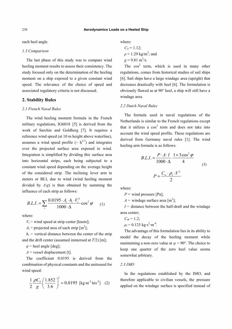
chosen for th

ti-aircraft frig

ided design)

a simplified

re not consid

nn [2] provide

of the supers

and its re

he hydrostatic

n Table 1.

namic App

ulae for wind

IMO) use the

t best taking

A

ition, the hee

th heel angl

1000

P A Z

g

⋅ ⋅=⋅ Δ ⋅

owindagesurf

the center of

derwater later

) [m].

ceptable as it

els like con

shape, have a

e heel angle.

ute an equiva

21

2 DC Vρ= ⋅

= 1.12;

coefficient.

his study is t

gate shown in

model of the

d superstruct

dered) as sh

es guidance on

structure on

ecommendati

c characterist

proach (I)

d heeling in t

aerodynamic

into account

Aerodynamic

eling momen

le. The B.L.I

face [Pa];

the windage

ral area (assu

applies mainl

ntainer ships

windage sur

alent wind sp

2PP

W

L BC ⋅

the French N

Fig. 1. The C

ship used for

ture (masts

hown in Fig

n the influenc

the aerodyna

ions have b

tics of the hul

the stability r

c drag at zero

t variation u

cs Loads on a

nt is

I. is

(4)

area

umed

ly to

s or

rface

peed

by

Com

obta

W

gus

kno

use

2.4

B

that

the

foll

1000

W

BA C

g

+ −

⋅ ⋅Δ

Navy

CAD

r this

and

g. 2.

ce of

amic

been

ll are

rules

heel

using

Fig.

Fig.

a Heeled Ship

comparing th

mparing with

ained is:

V

With the usua

t) and assumi

ots (IMO with

d in naval sta

Brown and D

Brown and

t considere

ship. Their

lows:

cos2

PPL B⋅

Δ

. 1 French fri

. 2 CAD mod

p

he IMO and n

h the French

0.019

PV =

al value of P

ing CY = 1.12

h gust) instea

ability rules fo

Deybach

Deybach [4

d the pri

wind heelin

s

2

BL

ϕ +

igate “Jean Ba

del of “Jean Ba

naval formula

h regulations,

5 g⋅

P = 504 Pa (I

2, then V = 5

ad of 100 kn

for combatant

4] proposed

incipal dim

ng arm form

cos2

BL ϕ−

art”.

art”.

239

a at zero heel.

the relation

(5)

IMO without

1 knots or 63

ots generally

ts.

d a formula

mensions of

mula was as

ϕ

(6)

9

.

n

)

t

3

y

a

f

s

)

Aerodynamics Loads on a Heeled Ship

240

Table 1 Main characteristics.

Lpp m 129.00

BWL m 14.00

T m 4.82 ∆ t 4873

LCG m 58.92

YG m 0.00

VCG m 5.96

Windage area m² 1346

Zaero m 6.24

Drift area m² 592

Zhydro/calm water plane m -2.37

cos2 or cos3 functions). In addition, they assume that

the drift center is located at half draft.

One way to improve upon these formulae is to

remove the assumption of an a-priori law of decrease

(cos2 or cos3) by calculating the actual projected

windage area and centroid height (Zaero) and immersed

lateral area and centroid depth (Zhydro) at each heel

angle. The wind heel lever formula is thus:

( ) 21

. . .2 1000

Y aero hydroC A Z Z VB L I

g

⋅ ⋅ − ⋅=

⋅Δ ⋅ (7)

where:

V = wind speed [m/s] (at height Zaero);

CY = 1.12;

ρ = 1.29 kg/m3;

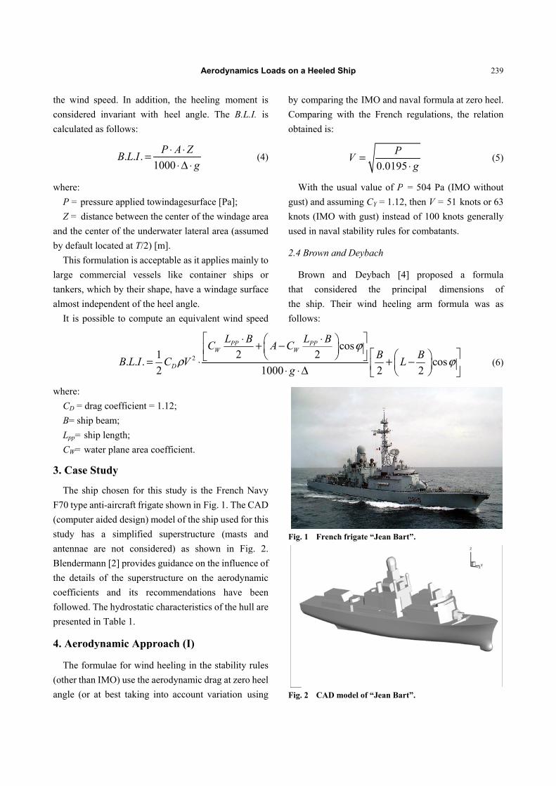
A, Zaero, Zhydro are calculated at each heel angle. This

is done by using FASTABI (DGA ydrodynamics code)

to establish the hull equilibrium position (waterline

position relative to hull) at each heel angle and then

using the CAD model to calculate projected areas and

centroids. Fig. 3 illustrates this procedure.

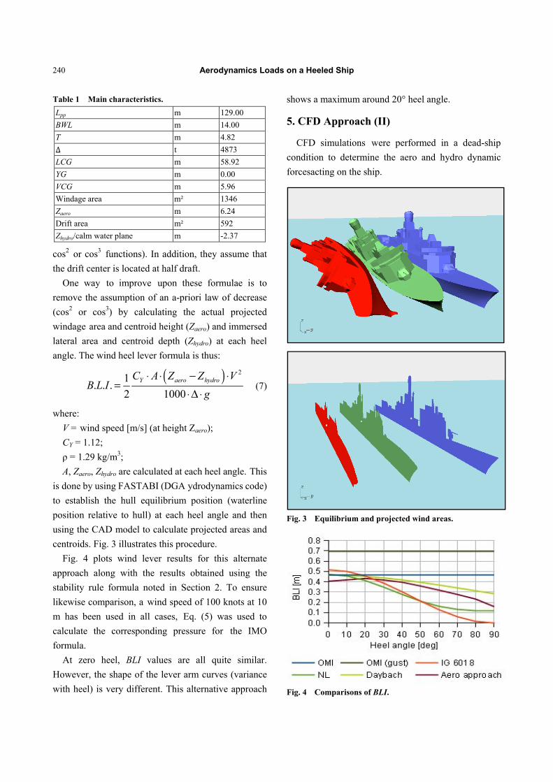
Fig. 4 plots wind lever results for this alternate

approach along with the results obtained using the

stability rule formula noted in Section 2. To ensure

likewise comparison, a wind speed of 100 knots at 10

m has been used in all cases, Eq. (5) was used to

calculate the corresponding pressure for the IMO

formula.

At zero heel, BLI values are all quite similar.

However, the shape of the lever arm curves (variance

with heel) is very different. This alternative approach

shows a maximum around 20° heel angle.

5. CFD Approach (II)

CFD simulations were performed in a dead-ship

condition to determine the aero and hydro dynamic

forcesacting on the ship.

Fig. 3 Equilibrium and projected wind areas.

Fig. 4 Comparisons of BLI.

Aerodynamics Loads on a Heeled Ship

241

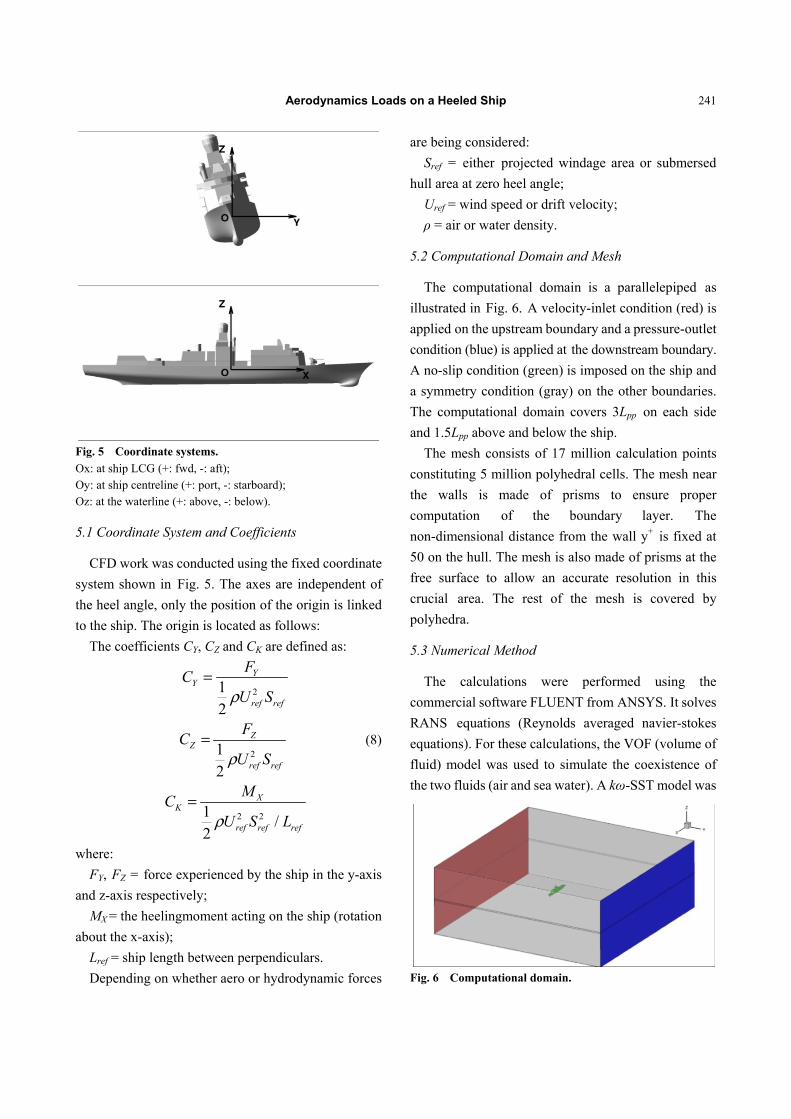
Fig. 5 Coordinate systems.

Ox: at ship LCG (+: fwd, -: aft); Oy: at ship centreline (+: port, -: starboard); Oz: at the waterline (+: above, -: below).

5.1 Coordinate System and Coefficients

CFD work was conducted using the fixed coordinate

system shown in Fig. 5. The axes are independent of

the heel angle, only the position of the origin is linked

to the ship. The origin is located as follows:

The coefficients CY, CZ and CK are defined as:

212

YY

ref ref

FC

U Sρ=

212

ZZ

ref ref

FC

U Sρ= (8)

2 21/

2

XK

ref ref ref

MC

U S Lρ=

where:

FY, FZ = force experienced by the ship in the y-axis

and z-axis respectively;

MX = the heelingmoment acting on the ship (rotation

about the x-axis);

Lref = ship length between perpendiculars.

Depending on whether aero or hydrodynamic forces

are being considered:

Sref = either projected windage area or submersed

hull area at zero heel angle;

Uref = wind speed or drift velocity;

ρ = air or water density.

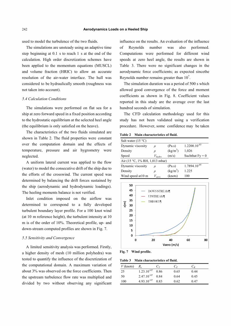
5.2 Computational Domain and Mesh

The computational domain is a parallelepiped as

illustrated in Fig. 6. A velocity-inlet condition (red) is

applied on the upstream boundary and a pressure-outlet

condition (blue) is applied at the downstream boundary.

A no-slip condition (green) is imposed on the ship and

a symmetry condition (gray) on the other boundaries.

The computational domain covers 3Lpp on each side

and 1.5Lpp above and below the ship.

The mesh consists of 17 million calculation points

constituting 5 million polyhedral cells. The mesh near

the walls is made of prisms to ensure proper

computation of the boundary layer. The

non-dimensional distance from the wall y+ is fixed at

50 on the hull. The mesh is also made of prisms at the

free surface to allow an accurate resolution in this

crucial area. The rest of the mesh is covered by

polyhedra.

5.3 Numerical Method

The calculations were performed using the

commercial software FLUENT from ANSYS. It solves

RANS equations (Reynolds averaged navier-stokes

equations). For these calculations, the VOF (volume of

fluid) model was used to simulate the coexistence of

the two fluids (air and sea water). A kω-SST model was

Fig. 6 Computational domain.

Aerodynamics Loads on a Heeled Ship

242

used to model the turbulence of the two fluids.

The simulations are unsteady using an adaptive time

step beginning at 0.1 s to reach 1 s at the end of the

calculation. High order discretization schemes have

been applied to the momentum equations (MUSCL)

and volume fraction (HRIC) to allow an accurate

resolution of the air-water interface. The hull was

considered to be hydraulically smooth (roughness was

not taken into account).

5.4 Calculation Conditions

The simulations were performed on flat sea for a

ship at zero forward speed in a fixed position according

to the hydrostatic equilibrium at the selected heel angle

(the equilibrium is only satisfied on the heave).

The characteristics of the two fluids simulated are

shown in Table 2. The fluid properties were constant

over the computation domain and the effects of

temperature, pressure and air hygrometry were

neglected.

A uniform lateral current was applied to the flow

(water) to model the consecutive drift of the ship due to

the efforts of the crosswind. The current speed was

determined by balancing the drift forces sustained by

the ship (aerodynamic and hydrodynamic loadings).

The heeling moments balance is not verified.

Inlet condition imposed on the airflow was

determined to correspond to a fully developed

turbulent boundary layer profile. For a 100 knot wind

(at 10 m reference height), the turbulent intensity at 10

m is of the order of 10%. Theoretical profile, up- and

down-stream computed profiles are shown in Fig. 7.

5.5 Sensitivity and Convergence

A limited sensitivity analysis was performed. Firstly,

a higher density of mesh (10 million polyhedra) was

tested to quantify the influence of the discretization of

the computational domain. A maximum variation of

about 3% was observed on the force coefficients. Then

the upstream turbulence flow rate was multiplied and

divided by two without observing any significant

influence on the results. An evaluation of the influence

of Reynolds number was also performed.

Computations were performed for different wind

speeds at zero heel angle, the results are shown in

Table 3. There were no significant changes in the

aerodynamic force coefficients; as expected sincethe

Reynolds number remains greater than 107.

The simulation duration was a period of 500 s which

allowed good convergence of the force and moment

coefficients as shown in Fig. 8. Coefficient values

reported in this study are the average over the last

hundred seconds of simulation.

The CFD calculation methodology used for this

study has not been validated using a verification

procedure. However, some confidence may be taken

Table 2 Main characteristics of fluid.

Salt water (15 °C)

Dynamic viscosity μ (Pa.s) 1.2200.10-03

Density ρ (kg/m3) 1,026

Speed Vhydro (m/s) Suchthat Fy = 0

Air (15 °C, 1% RH, 1,013 mbar)

Dynamic viscosity μ (Pa.s) 1.7894.10-05

Density ρ (kg/m3) 1.225

Wind speed at10 m Vaero (knots) 100

Fig. 7 Wind profile.

Table 3 Main characteristics of fluid.

V (knots) Re CY CZ CK

25 1.23.10+07 0.86 0.65 0.44

50 2.47.10+07 0.84 0.64 0.45

100 4.93.10+07 0.83 0.62 0.47

Aerodynamics Loads on a Heeled Ship

243

Fig. 8 Force and moment time trace.

from comparison of the results obtained to data from

wind tunnel tests. Blendermann [2, 3] conducted zero

heel angle tests for two ships with silhouettes similar to

that of the F70 frigate (see Fig. 9). Table 4 presents the

CY and CK coefficients from CFD and the Blendermann

tests.

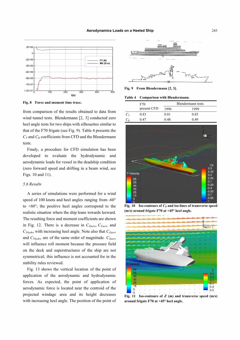
Finaly, a procedure for CFD simulation has been

developed to evaluate the hydrodynamic and

aerodynamic loads for vessel in the deadship condition

(zero forward speed and drifting in a beam wind, see

Figs. 10 and 11).

5.6 Results

A series of simulations were performed for a wind

speed of 100 knots and heel angles ranging from -60°

to +60°; the positive heel angles correspond to the

realistic situation where the ship leans towards leeward.

The resulting force and moment coefficients are shown

in Fig. 12. There is a decrease in CZaero, CYaero and

CYhydro with increasing heel angle. Note also that CZaero

and CYhydro are of the same order of magnitude. CZaero

will influence roll moment because the pressure field

on the deck and superstructures of the ship are not

symmetrical; this influence is not accounted for in the

stability rules reviewed.

Fig. 13 shows the vertical location of the point of

application of the aerodynamic and hydrodynamic

forces. As expected, the point of application of

aerodynamic force is located near the centroid of the

projected windage area and its height decreases

with increasing heel angle. The position of the point of

Fig. 9 From Blendermann [2, 3].

Table 4 Comparison with Blendermann.

F70 present CFD

Blendermann tests

1996 1999

CY 0.83 0.81 0.85

CK 0.47 0.48 0.49

Fig. 10 Iso-contours of CP and iso-lines of transverse speed (m/s) around frigate F70 at +45° heel angle.

Fig. 11 Iso-contours of Z (m) and transverse speed (m/s) around frigate F70 at +45° heel angle.

Aerodynamics Loads on a Heeled Ship

244

Fig. 12 Force and moment coefficients for different heel angles.

Fig. 13 Vertical location of hydro and aero forces.

application of hydrodynamic forces is above the free

surface at zero heel but moves below with increasing

heel angle to approach the mid-draft position. The

Table 5 Drifting speeds for 100 knots of wind.

Heel (°)

CY hydro (-)

CY aero (-)

Vhydro (knots)

-60 0.65 0.78 5.7

-45 0.69 0.78 5.6

-30 0.85 0.77 5.0

-15 0.73 0.75 5.3

0 0.72 0.83 5.6

15 0.72 0.83 5.6

30 0.69 0.85 5.8

45 0.68 0.78 5.6

60 0.65 0.72 5.5

Fig. 14 BLI comparisons.

heeling moment lever arm, z (aero)-z (hydro), does not

change greatly with heel angle.

Table 5 presents drift velocity (Vhydro) and the lateral

force coefficients CYhydro and CYaero for each heel angle.

There are little variations in CYhydro and CYaero and thus

Vhydro over the range of heel angles.

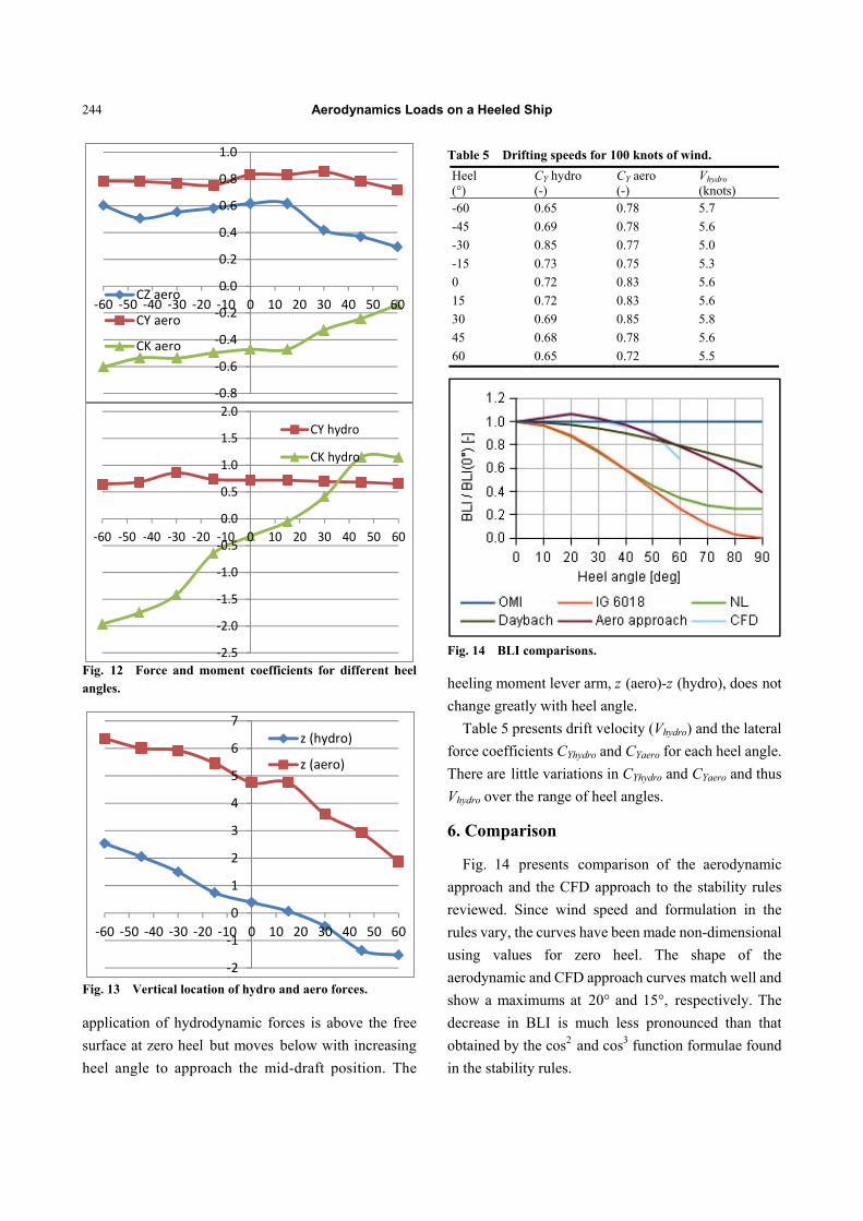
6. Comparison

Fig. 14 presents comparison of the aerodynamic

approach and the CFD approach to the stability rules

reviewed. Since wind speed and formulation in the

rules vary, the curves have been made non-dimensional

using values for zero heel. The shape of the

aerodynamic and CFD approach curves match well and

show a maximums at 20° and 15°, respectively. The

decrease in BLI is much less pronounced than that

obtained by the cos2 and cos3 function formulae found

in the stability rules.

-2

-1

0

1

2

3

4

5

6

7

-60 -50 -40 -30 -20 -10 0 10 20 30 40 50 60

z (hydro)

z (aero)

-0.8

-0.6

-0.4

-0.2

0.0

0.2

0.4

0.6

0.8

1.0

-60 -50 -40 -30 -20 -10 0 10 20 30 40 50 60CZ aero

CY aero

CK aero

-2.5

-2.0

-1.5

-1.0

-0.5

0.0

0.5

1.0

1.5

2.0

-60 -50 -40 -30 -20 -10 0 10 20 30 40 50 60

CY hydro

CK hydro

Aerodynamics Loads on a Heeled Ship

245

7. Conclusions

A review was made of different stability rule

formulae to account for the effects of wind heeling.

These formulae have been applied to the case of F70

frigate. The results obtained were compared to those

derived from two alternate approaches. The first

approach adopted the same basic formula of the

stability rules but replaced the fixed upright windage

area, centroids and cos2 terms with actual areas and

centroids determined for each heel angle. The second

approach employed CFD analysis to determine force

and moment coefficients at each heel angle. A

procedure for CFD simulation has been developed to

evaluate the hydrodynamic and aerodynamic loads for

vessel in the deadship condition (zero forward speed

and drifting in a beam wind).

For the F70 frigate, the two alternate approaches

produced similar BLI results. The BLI versus heel

angle curves for both have a significantly different

shape than that derived from stability rule formula

based on a cos2 law. Of particular note is that both

approaches show a peak in BLI (maximum

destabilizing moment) in the 15° to 20° range of heel.

The alternate approaches presented here are

interesting and deserve further study. In particular,

further work can be done to improve the accuracy of

the CFD simulations and validate the results obtained.

This would provide the tool necessary for more

comprehensive analysis leading to improved stability

rule formulae.

Acknowledgments

This study was based on CRNAV (Cooperative

Research Navies) discussions. Thanks also to Hélène

Eudier who started the work in Val de Reuil during a

training course. For the French part, the study is found

by the French Ministry of Defence to support DGA

Hydrodynamics in its research activities.

References

[1] Arndt, B., Brandl, H., and Vogt, K. 1982. “20 Years of

Experience—Stability Regulations of the West-German

Navy.” Presented at STAB’82, Tokyo, 111-21.

[2] Blendermann, W. 1999. “Influence of Model Details on

the Wind Loads Demonstrated on a Frigate.”

Schiff&Hafen.

[3] Blendermann, W. 1996. Wind Loadings of

Ships—Collected Data from Wind Tunnel Tests in

Uniform Flow. Report 574. Institute of Naval

Architecture.

[4] Brown, A. J., and Deybach, F. 1998. “Towards a Rational

Intact Stability Criteria for Naval Ships.” Naval Engineers

Journal 110: 65-77.

[5] DGA/DSA/SPN IG 6018 Indice A. 1999. Stabilité des

Bâtiments de la Marine. (in French)

[6] Middendorf. 1903. Bemastung und Takelung des Schiffe.

MSC.267(85). (in German)

[7] Sarchin & Goldberg. 1962. “Stability and Buoyancy

Criteria for US Naval Surface Ship.” SNAME

Transactions 70: 418-34.