Ae11 sol
62
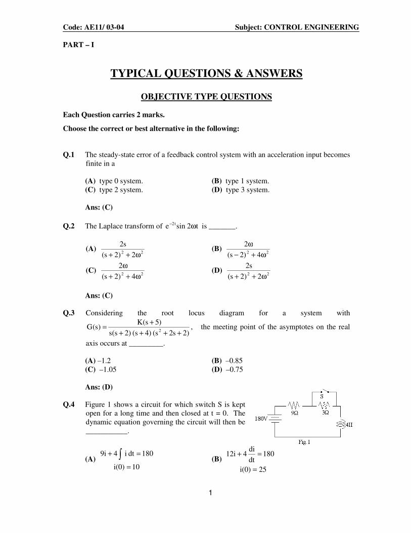
Code: AE11/ 03-04 Subject: CONTROL ENGINEERING 1 PART – I TYPICAL QUESTIONS & ANSWERS OBJECTIVE TYPE QUESTIONS Each Question carries 2 marks. Choose the correct or best alternative in the following: Q.1 The steady-state error of a feedback control system with an acceleration input becomes finite in a (A) type 0 system. (B) type 1 system. (C) type 2 system. (D) type 3 system. Ans: (C) Q.2 The Laplace transform of t 2 sin e t 2 ω - is _______. (A) 2 2 2 ) 2 s ( s 2 ω + + (B) 4 ) 2 s ( 2 2 2 ω + - ω (C) 4 ) 2 s ( 2 2 2 ω + + ω (D) 2 ) 2 s ( s 2 2 2 ω + + Ans: (C) Q.3 Considering the root locus diagram for a system with ) 2 s 2 (s 4) (s ) 2 s ( s ) 5 s ( K ) s ( G 2 + + + + + = , the meeting point of the asymptotes on the real axis occurs at _________. (A) –1.2 (B) –0.85 (C) –1.05 (D) –0.75 Ans: (D) Q.4 Figure 1 shows a circuit for which switch S is kept open for a long time and then closed at t = 0. The dynamic equation governing the circuit will then be ___________. (A) 10 i(0) 180 dt i 4 9i = = + ∫ (B) 25 i(0) 180 dt di 4 12i = = +
-
Upload
lecturer-in-mit -
Category
Documents
-
view
255 -
download
0
Transcript of Ae11 sol
Code: AE11/ 03-04 Subject: CONTROL ENGINEERING
1
PART – I
TYPICAL QUESTIONS & ANSWERS
OBJECTIVE TYPE QUESTIONS
Each Question carries 2 marks.
Choose the correct or best alternative in the following:
Q.1 The steady-state error of a feedback control system with an acceleration input becomes
finite in a (A) type 0 system. (B) type 1 system. (C) type 2 system. (D) type 3 system.
Ans: (C)
Q.2 The Laplace transform of t 2sin e t2 ω− is _______.
(A) 22 2)2s(
s2
ω++ (B)
4)2s(
222 ω+−
ω
(C) 4)2s(
222 ω++
ω (D)
2)2s(
s222 ω++
Ans: (C)
Q.3 Considering the root locus diagram for a system with
)2s2(s 4)(s )2s(s
)5s(K)s(G
2 ++++
+= , the meeting point of the asymptotes on the real
axis occurs at _________. (A) –1.2 (B) –0.85 (C) –1.05 (D) –0.75 Ans: (D) Q.4 Figure 1 shows a circuit for which switch S is kept
open for a long time and then closed at t = 0. The dynamic equation governing the circuit will then be ___________.
(A) 10i(0)
180dt i49i
=
=+ ∫ (B)
25i(0)
180dt
di 412i
=
=+
Code: AE11/ 03-04 Subject: CONTROL ENGINEERING
2
(C)
15i(0)
180dt
di 49i
=
=+ (D)
15i(0)
180dt i 412i
=
=+ ∫
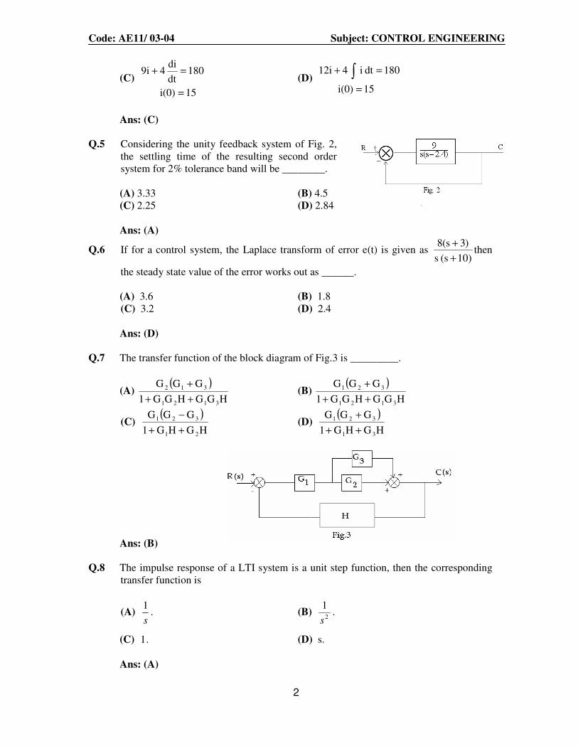
Ans: (C) Q.5 Considering the unity feedback system of Fig. 2,
the settling time of the resulting second order system for 2% tolerance band will be ________.
(A) 3.33 (B) 4.5 (C) 2.25 (D) 2.84 Ans: (A)
Q.6 If for a control system, the Laplace transform of error e(t) is given as )10s( s
)3s(8
+
+then
the steady state value of the error works out as ______. (A) 3.6 (B) 1.8 (C) 3.2 (D) 2.4
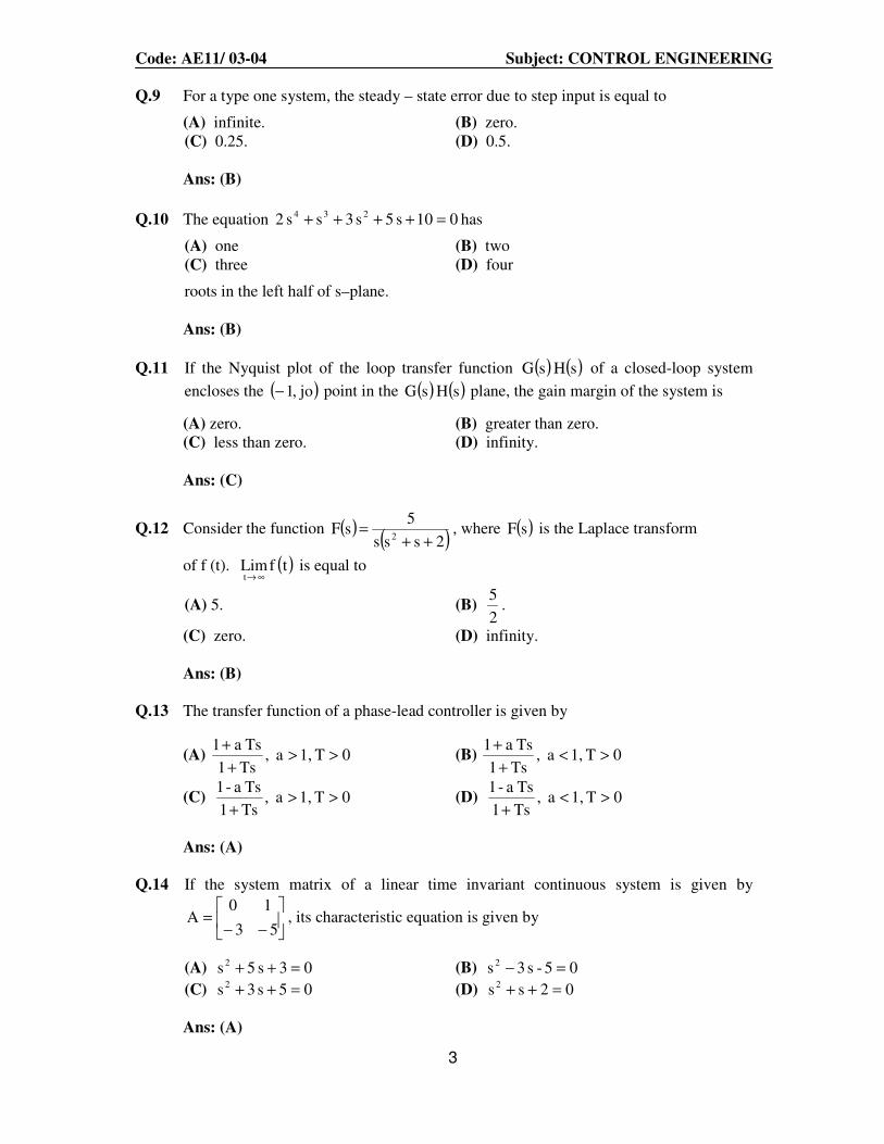
Ans: (D) Q.7 The transfer function of the block diagram of Fig.3 is _________.
(A) ( )
HGGHGG1
GGG
3121
312
++
+ (B)
( )HGGHGG1
GGG
3121
321
++
+
(C) ( )
HGHG1
GGG
21
321
++
− (D)
( )HGHG1
GGG
31
321
++
+
Ans: (B)
Q.8 The impulse response of a LTI system is a unit step function, then the corresponding transfer function is
(A) s
1. (B)
2
1
s.
(C) 1. (D) s.
Ans: (A)
Code: AE11/ 03-04 Subject: CONTROL ENGINEERING
3
Q.9 For a type one system, the steady – state error due to step input is equal to
(A) infinite. (B) zero. (C) 0.25. (D) 0.5.
Ans: (B)
Q.10 The equation 010s 5s 3ss 2 234 =++++ has
(A) one (B) two (C) three (D) four
roots in the left half of s–plane.
Ans: (B)
Q.11 If the Nyquist plot of the loop transfer function ( ) ( )sH sG of a closed-loop system
encloses the ( )jo,1− point in the ( ) ( )sH sG plane, the gain margin of the system is
(A) zero. (B) greater than zero. (C) less than zero. (D) infinity.
Ans: (C)
Q.12 Consider the function ( )( )2sss
5 sF
2 ++= , where ( )sF is the Laplace transform
of f (t). ( )tfLim t ∞→
is equal to
(A) 5. (B) 2
5.
(C) zero. (D) infinity.
Ans: (B) Q.13 The transfer function of a phase-lead controller is given by
(A) 0T 1,a ,Ts1
Ts a1>>
+
+ (B) 0T 1,a ,
Ts1
Ts a1><
+
+
(C) 0T 1,a ,Ts1
Ts a-1>>
+ (D) 0T 1,a ,
Ts1
Ts a-1><
+
Ans: (A) Q.14 If the system matrix of a linear time invariant continuous system is given by
−−=
53
10A , its characteristic equation is given by
(A) 03s 5s 2 =++ (B) 05-s 3s 2 =−
(C) 05s 3s 2 =++ (D) 02s s 2 =++
Ans: (A)

Code: AE11/ 03-04 Subject: CONTROL ENGINEERING
4
Q.15 Given a unity feedback control system with ( )( )
,4ss
KsG
+= the value of K for a
damping ratio of 0.5 is
(A) 1. (B) 16. (C) 32. (D) 64.
Ans: (B)
Q.16 Given ( ) ( ) ( )[ ]ate tf L,sFtf L −= is equal to
(A) ( )asF + . (B) ( )
( )as
sF
+.
(C) ( )sFeas . (D) ( )sFe-as .
Ans: (A) Q.17 The state-variable description of a linear autonomous system is
XAX.
=
Where X is a two-dimensional state vector and A is a matrix given by
=
0 2
2 0A
The poles of the system are located at (A) -2 and +2 (B) -2j and +2j (C) -2 and -2 (D) +2 and +2 Ans: (A) Q.18 The LVDT is primarily used for the measurement of
(A) displacement (B) velocity (C) acceleration (D) humidity Ans: (A)
Q.19 A system with gain margin close to unity or a phase margin close to zero is
(A) highly stable. (B) oscillatory. (C) relatively stable. (D) unstable. Ans: (C)
Q.20 The overshoot in the response of the system having the transfer function
( )16s 2ss
K 162 ++
for a unit-step input is
(A) 60%. (B) 40%. (C) 20%. (D) 10%. Ans: (B)

Code: AE11/ 03-04 Subject: CONTROL ENGINEERING
5
Q.21 The damping ratio of a system having the characteristic equation
08s2s 2 =++ is (A) 0.353 (B) 0.330. (C) 0.300 (D) 0.250. Ans: (A) Q.22 The input to a controller is (A) sensed signal. (B) desired variable value. (C) error signal. (D) servo-signal. Ans: (C)
Q.23 If the transfer function of a first-order system is s21
10)s(G
+= , then the time constant
of the system is
(A) 10 seconds. (B) 10
1 second.
(C) 2 seconds. (D) 2
1 second.
Ans: (C) Q.24 The unit-impluse response of a system starting from rest is given by
0for t e1C(t) 2t ≥−= −
The transfer function of the system is
(A) s21
1
+ (B)
2s
2
+
(C) )2s(s
2
+ (D)
2s
1
+
Ans: (C)
Q.25 Closed-loop transfer function of a unity-feedback system is given by
( ) ( ) ( )1s1sRsY +τ= . Steady-state error to unit-ramp input is
(A) ∞ (B) τ
(C) 1 (D) τ1
Ans: (B)

Code: AE11/ 03-04 Subject: CONTROL ENGINEERING
6
Q.26 Electrical time-constant of an armature-controlled dc servomotor is (A) equal to mechanical time-constant. (B) smaller than mechanical time-constant. (C) larger than mechanical time-constant. (D) not related to mechanical time-constant.
Ans: (B) Q.27 In the system of Fig.1, sensitivity of
)s(R)s(Y)s(M = with respect to
parameter 1K is
(A)21KK1
1
+
(B))s(GK1
1
1+
(C) 1
(D) None of the above.
Ans: (C) Q.28 The open-loop transfer function of a unity feedback system is
[ ] 0K; )5s(sK)s(G 2 >+=
The system is unstable for (A) K>5 (B) K<5 (C) K>0 (D) all the above.
Ans: (D) Q.29 Peak overshoot of step-input response of an underdamped second-order system is
explicitly indicative of (A) settling time. (B) rise time. (C) natural frequency. (D) damping ratio.
Ans: (D)
Q.30 A unity feedback system with open-loop transfer function [ ])(4)( psssG += is
critically damped. The value of the parameter p is (A) 4. (B) 3. (C) 2. (D) 1. Ans: (A)

Code: AE11/ 03-04 Subject: CONTROL ENGINEERING
7
Q.31 Consider the position control system of Fig.2. The value of K such that the steady-
state error is °10 for input 400tθ r = rad/sec, is
(A) 104.5 (B) 114.5 (C) 124.5 (D) None of the above.
Ans: (B)
Q.32 Polar plot of [ ])j1(j1)j(G ωτ+ω=ω
(A) crosses the negative real axis. (B) crosses the negative imaginary axis. (C) crosses the positive imaginary axis. (D) None of the above.
Ans: (D)

Code: AE11/ 03-04 Subject: CONTROL ENGINEERING
8
PART – II
NUMERICALS
Q.1 Write the dynamic equation in respect of the mechanical system given in Fig.4. Then using force-voltage analogy obtain the equivalent electrical network.
Legend
21 K,K spring constants
1B viscous friction damping coefficient
21 M,M inertial constants of masses
21 x,x displacements
F (t) .. Force. (14)
Ans :
From figure, a force F(t) is applied to mass M2.
Free body diagrams for these two masses are

Code: AE11/ 03-04 Subject: CONTROL ENGINEERING
9
From these, the following differential equations describing the dynamics of the system.
F(t) - K2( 2X - 1X ) =M2 2X••
K2 ( 2X -1X ) –K1 1X – B1 1X
•
=M1 1X••
From above we can write down
M2 2X••
+ K2( 2X - 1X ) = F(t)
M1 1X••
+ K1 1X + B1 1X•
- K2 ( 2X -1X ) = 0;
These two are simultaneous second order linear differential equations. Manipulation of these equations results in a single differential equations relating the response X2 (or X1) to input F(t).
Electrical Analogous for the circuit:

Code: AE11/ 03-04 Subject: CONTROL ENGINEERING
10
The dynamic equations of the system could also be obtained by writing nodal equations for the electrical network.
f 1 1V + K1 1
t
V−∞∫ dt 11M V
•
+ + K2 1 2( )t
V V−∞
−∫ dt = 0;
M2 2V•
+ K2 1 2( )t
V V−∞
−∫ dt = F(t)
Force Voltage Analogy:
The dynamical equations of the system could also obtained by writing nodal equations for electrical network.
K1 1
t
i−∞
∫ dt + R1 i1 + M1 1i•
+ K2 1 2( )t
i i−∞
−∫ dt = 0;
M2 i2 + K2 1 2( )t
i i−∞
−∫ dt = F(t)
Q.2 Determine the transfer function ( )
)s(R
sC for the block diagram shown in Fig.5 by first
drawing its signal flow graph and then using the Mason’s gain formula. (14)
Code: AE11/ 03-04 Subject: CONTROL ENGINEERING
11
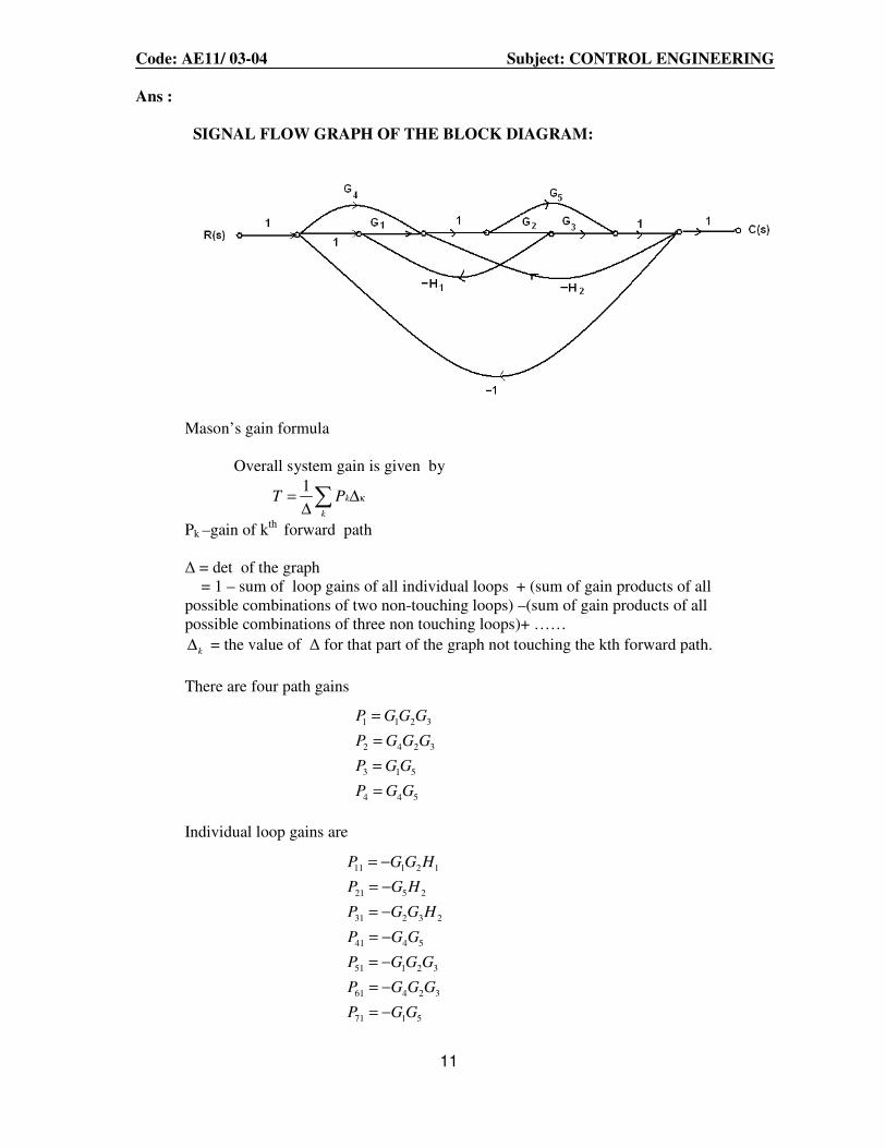
Ans : SIGNAL FLOW GRAPH OF THE BLOCK DIAGRAM:
Mason’s gain formula Overall system gain is given by
1
k
k
T P κ= ∆∆∑
Pk –gain of kth forward path ∆ = det of the graph = 1 – sum of loop gains of all individual loops + (sum of gain products of all possible combinations of two non-touching loops) –(sum of gain products of all possible combinations of three non touching loops)+ ……
k∆ = the value of ∆ for that part of the graph not touching the kth forward path.
There are four path gains
1 1 2 3
2 4 2 3
3 1 5
4 4 5
P G G G
P G G G
P G G
P G G
=
=
=
=
Individual loop gains are
11 1 2 1
21 5 2
31 2 3 2
41 4 5
51 1 2 3
61 4 2 3
71 1 5
P G G H
P G H
P G G H
P G G
P G G G
P G G G
P G G
= −
= −
= −
= −
= −
= −
= −

Code: AE11/ 03-04 Subject: CONTROL ENGINEERING
12
There are no non touching loops ∆ = 1-(- G1G2H1-G5H2-G2G3H2-G4G5-G1G2G3-G4G2G3-G1G5) P1 ∆1 + P2 ∆2 + P3 ∆3 +P4 ∆4 T = ------------------------------------------ ∆ G1G2G3 + G4G2G3 +G1G5 + G4G5 = ------------------------------------------------------------------------- 1+ G1G2H1+G5H2+G2G3H2+G4G5+G1G2G3+G4G2G3+G1G5
Q.3 The open loop transfer functions of three systems are given as
(i) ( )( )2s1s
4
++ (ii)
( )( )6s4ss
2
++ (iii)
( )( )10s3ss
52 ++
Determine respectively the positional, velocity and acceleration error constants for these systems. Also for the system given in (ii) determine the steady state errors
with step input )t(u)t(r = , ramp input r(t) = t and acceleration input 2t2
1)t(r = . (10)
Ans :
4 (i) ---------------- (s+1)(s+2) Positional error for unit step input 1 1 1
sse = lim ----------- = ----------- = ------------
s→0 1 + G(s) 1 + G(0) 1 + pk
pk = G(0) is defined as positional error constant
pk = 4/2 = 2 sse = 1/3
vk = lim s G(s) is defined as velocity error constant 0
*4lim 0
( 1)( 2)s
s
s s→= =
+ +
s→0 velocity error for ramp input 1 1 1
sse = lim ---------------- = lim ------ = ------- = ∞
s→0 s( 1 + G(0)) s→0 sG(s) vk
Acceleration error constant
ak = lim s2 G(s) is defined as velocity error constant 2
0
*4lim 0
( 1)( 2)s
s
s s→= =
+ +
s→0
Code: AE11/ 03-04 Subject: CONTROL ENGINEERING
13
1 1 1
sse = lim ------------- = lim --------- = ------- = ∞
s→0 s2(1+G(s)) s→0 s2G(s) ak
(ii)
pk = lim G(s)H(s)
s→0 2 = lim ------------------ = ∞ s→0 s(s+4)(s+6) 2s 2 1
vk = lim sG(s)H(s) = lim ---------------- = ------ = ------
s→0 s→0 s(s+4)(s+6) 24 12 2s2
ak = lim s2G(s)H(s) = lim --------------- = 0
s→0 s→0 s(s+4)(s+6) 5 (iii) ------------------- s2(s+3)(s+10)
pk = lim G(s)H(s)
s→0 5 = lim ------------------ = ∞ s→0 s2(s+3)(s+10) 5 s
vk = lim sG(s)H(s) = lim ---------------- = ∞
s→0 s→0 s2(s+3)(s+10) 5 s2 1
ak = lim s2G(s)H(s) = lim --------------- = ------
s→0 s→0 s2(s+3)(s+10) 6 taking the second system, 2 ------------------- s(s+4)(s+6) step input u(t)
Code: AE11/ 03-04 Subject: CONTROL ENGINEERING
14
1 1
sse = ---------- = ----------- = 0
1 + pk 1 + ∞
Ramp input t 1
sse = ------ = 12
vk
parabola input t2/2 1
sse = ----- = ∞
ak
Q.4 Describe a two phase a.c. servomotor and derive its transfer function. (4)
Ans :
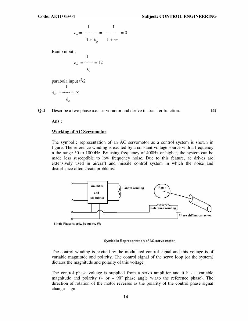
Working of AC Servomotor: The symbolic representation of an AC servomotor as a control system is shown in figure. The reference winding is excited by a constant voltage source with a frequency n the range 50 to 1000Hz. By using frequency of 400Hz or higher, the system can be made less susceptible to low frequency noise. Due to this feature, ac drives are extensively used in aircraft and missile control system in which the noise and disturbance often create problems.
The control winding is excited by the modulated control signal and this voltage is of variable magnitude and polarity. The control signal of the servo loop (or the system) dictates the magnitude and polarity of this voltage. The control phase voltage is supplied from a servo amplifier and it has a variable magnitude and polarity (+ or – 90o phase angle w.r.to the reference phase). The direction of rotation of the motor reverses as the polarity of the control phase signal changes sign.

Code: AE11/ 03-04 Subject: CONTROL ENGINEERING
15
It can be proved that using symmetrical components that the starting torque of a servo-motor under unbalanced operation is proportional to E, the rms value of the sinusoidal control voltage e(t) . A family of torque-speed characteristics curves with variable rms control voltage is shown in figure. All these curves have negative slope.
Note that the curve for zero control voltage goes through the origin and the motor develops a decelerating torque. From the torque speed characteristic shown above we can write
n c c
dT k k e
dt
θ= − + (1)
Where T = torque
nk = a positive constant = -ve of the slope of the torque-speed curve
ck = a positive constant = torque per unit control voltage at zero speed
θ = angular displacement Further, for motor we have
2
2
d dT J f
dt dt
θ θ= + (2)
Where J = moment of inertia of motor and load reffered to motor shaft f = viscous friction coefficient of the motor and load referred to the motor shaft form eqs.(1) and (2) we have
2
2
d dJ f
dt dt
θ θ+ =
n c c
dk k e
dt
θ− +

Code: AE11/ 03-04 Subject: CONTROL ENGINEERING
16
2
2( )n c c
d dJ f k k e
dt dt
θ θ+ + = (3)
Taking the laplace transform on both sides, putting initial conditions zero and simplifying we get
2
( )
( ) ( ) ( 1)c m
c n m
k ks
E s Js f k s s s
θ
τ= =
+ + + (4)
Where
( )c
m
n
kk
f k=
+= motor gain constant
If the moment of inertia J is small. Then mτ is small and for the frequency range of
relevance to ac servometer 1msτ << ,then from eq (4) we can write the transfer
function as
( )
( )m
c
ks
E s s
θ= (5)
It means that ac servometer works as an integrator. Following figure gives the simplified block diagram of an ac servometer.
Q.5 For the system shown in the block diagram of Fig.7 determine the values of gain
1K and velocity feedback constant 2K so that the maximum overshoot with a unit
step input is 0.25 and the time to reach the first peak is 0.8 sec. Thus obtain the rise time and settling time for 5% tolerance band. (10)
( 1)m
m
k
s sτ +
( )cE s ( )sθ

Code: AE11/ 03-04 Subject: CONTROL ENGINEERING
17
Ans :
k1/(s(s+2) M(s) = ------------------------------- 1 + k1(1 + k2s)/(s(s+2)) k1 k1 = -------------------------------- = ------------------------------ s2 + 2s + k1 + k1k2s s2 + (2 + k1k2)s + k1 peak over shoot = 0.25 = e –ξ π /( 1- ξ 2)1/2
ξ = 0.403 π
pt = 0.8 sec = ----------------------
nw ( 1- ξ2 )1/2
nw = 4.29 rad/sec
1k =nw
2 = 18.4
(2 + 1k 2k ) =2 ξ nw = 3.457
1k 2k = 1.457 2k = 0.079
π – 1tan− ((1- ξ2)1/2/ ξ)
rt = ------------------------------------ = 0.505 sec
nw ((1- ξ2)1/2)
st = 3/ ξ nw = 1.735 sec
Q.6 For the standard second order system shown in Fig.8, with r (t) = u (t) explain how the time domain specifications corresponding to resonant peak and bandwidth can be inferred. (4)

Code: AE11/ 03-04 Subject: CONTROL ENGINEERING
18
Ans :
C(s) nw2
----- = ---------------------------
R(s) s2 + 2 ξnw s+
nw2
1 M(jw) = -------------------------------
(1-w2/ nw2) + j2 ξ(w/ nw )
1
2M = -----------------------------
(1-w2/nw
2)2 + 4 ξ2( 2w /
nw2)
d 2M -4(1-w2/ nw2)(w/ nw
2) + 8 ξ2(w/ nw2)
------ = -----------------------------------------------------
dw [(1-w2/nw
2)2 + 4 ξ2(w2/nw
2)]2
rw = nw (1-2 ξ2)1/2
for this.,
1
rM = -----------------
2 ξ( 1- ξ2)1/2
Band width For M = 1/1.414 is BW 1
----------------------------------------- = 1
2
(1- bw2/ nw
2)2 + 4 ξ2( bw2/ nw
2)
( bw4/ nw
4) -2(1-2 ξ2)( bw2/ nw
2) – 1 = 0
bw2/
nw2 = (1-2 ξ2) ± (4 ξ4 - 4 ξ2 +2)1/2
bw = nw ( (1-2 ξ2) + (4 ξ4 -4 ξ2 + 2)1/2)1/2)

Code: AE11/ 03-04 Subject: CONTROL ENGINEERING
19
Q.7 The characteristic equation of a closed loop control system is given as
024s50s35s10s 234 =++++ . For this system determine the number of roots to the right of the vertical axis located at s = - 2. (10)
Ans : s4 +10s3 +35s2 +50s +24 = 0
shift origin s = -2 so, s = z-2 (z-2)4 + 10(z-2)3 + 35(z-2)2 + 50(z-2) + 24 = (z2 + 4 -4z)2 + 10(z3 -6z2+12z -8) + 35(z2 + 4 – 4z) + 50z -100 +24 = z4 + 16 + 16z2 +8z2 – 32z – 8z3 + 10z3 -80 – 60z2 +120z +35z2 -140z +140-50z - 100+24 =z4 +2z3 –z2 – 2z = 0
z4 1 -1 0
z3 2 -2 0
z2 0 0
A(z) = 2z3 – 2z dA(z) -------- = 6z2 – 2 dz
z3 2 -2 0
z2 3 -1 0
z1 -4/3
z0 -1
There is one sign change so one root to right of s = -2
Q.8 Draw the complete Nyquist plot for a unity feed back system having the open loop
function ( )( )( )s6s5.01s
6sG
++= . From this plot obtain all the information
regarding absolute as well as relative stability. (14)

Code: AE11/ 03-04 Subject: CONTROL ENGINEERING
20
Ans :
6 G(s)H(s) = ---------------------- s(1+0.5s)(6+s)
G(jw) at w = 0 = 090∞∠ − G(jw) at w→∞ = 00 90∠
2
6( )
(0.5 )( 6)s jw
G jws s s
=
=+ +
6 = ---------------------------- = 6(-0.5w2 – jw) (-0.5w2 + jw)(jw + 6) Nyquist contour is given by Semicircle around the origin represented by
0
jS e
θεε →=
θ varying from -900 through 00 to 900 Maps into 6 Lim --------------------------------------- = ∞
ε →0 6 ε je θ (1+0.5 je θ )(1+1/6 je θ ) -900 through 00 to 900 mapping of positive imaginary axis (w =0+ to ∞+) calculate magnitude and phase values of T.F 6 ---------------------------- at various values of w 6jw(1+0.5jw)(1+1/6jw)
1 10 50 100 500
magnitude -1.085 -39.89 -80.389 -98.39 -140.32
phase 234 132.37 99.16 94.59 90.91
Mapping of infinite semicircular arc of the nyquist contour represented by
Re jS
θ= (θ varying from +90 through 0 to -90 as R→ ∞)
1
Re (1 0.5Re )(1 0.166 Re )R j j j
Limθ θ θ→∞=
+ +
= 0 e-j3 Ǿ

Code: AE11/ 03-04 Subject: CONTROL ENGINEERING
21
-2700 through 00 to -2700
NYQUIST PLOT
The system is stable and the relative stability is represented by phase margin and gain margin. Gain margin = 18.1 ,Phase cross frequency = 3.46 rad/sec. Phase margin = 57.2 , Gain cross frequency = 0.902 rad/sec
Q.9 Sketch the root locus diagram for a unity feedback system with its open loop
function as ( ) ( )( )( )( )9s5s2s2ss
3sKsG
2 ++++
+= . Thus find the value of K at a point
where the complex poles provide a damping factor of 0.5. (14)
Ans :
K(s + 3) G(s) = ------------------------------------- s(s2 +2s +2)(s+5)(s+9) Location of poles and zeros
s2 +2s +2 = 0 2 (4 8)
2s
− ± −= = -1± j1
poles s=0, -1±j1, -5,-9 zeros s = -3

Code: AE11/ 03-04 Subject: CONTROL ENGINEERING
22
±180(2q + 1) angle of asympototes = ----------------- (n – m) n =5, m = 1 ± 45 , ± 135 -5-9-1-1-(-3) centroid = ------------------ = -13/4 4 Break away point C(S) k(s+3) ----- = ---------------------------------------- R(s) s(s2 + 2s+2)(s+5)(s+9) +k(s+3) Characterstic equation; (s3 + 2s2 + 2s)(s2 + 14s +45) + k(s+3) =0 s5 +14s4 +45s3 +2s4 +28s3 +90s2 +2s3 +28s2 +90s)+k(s+3) =0 -(s5 +16s4 +75s3 +118s2+90s) k = ---------------------------------------- (s+3) dk -(s+3)(5s4 +64s3+22s2+236s+90)+(s5+16s4+75s3+118s2+90s) ---- = ----------------------------------------------------------------------------- = 0 ds (s+3)2 (4s5+63s4+342s3+793s2+708s+270)=0 s = -7.407, -3.522±j1.22,-0.64±j0.48 -7.4 is the breaking point Angle of departure at A
1φ =900
2φ = 1800-tan-1(1/1) = 1350
3φ = tan-1(1/4) = 14.030
4φ = tan-1(1/8) = 7.1250
A = tan-1 (1/2)= 26.560 1800 – (900+1350+14.030+7.1250) +26.560= -39.60 A* =39.60 To find k at ξ =0.5

Code: AE11/ 03-04 Subject: CONTROL ENGINEERING
23
α = cos-10.5 =60 product of length of vector from all poles to point value of k =-------------------------------------------------------------- product of length from all zeros to point = 14.7
Figure: Root Locus Diagram
Q.10 Obtain the transfer function of the two-phase servo–motor whose torque–speed curve is shown in Fig.2. The maximum rated fixed-phase and control–phase voltages are 115 volts. The moment of inertia of the motor (including the effect of load) is
-4107.77× Kgm- 2m . Motor friction (including the effect of load) is negligible. (7+7)
Code: AE11/ 03-04 Subject: CONTROL ENGINEERING
24
Ans : The transfer function of a two phase servo motor is given by Ө(s) kc ----------- = ----------------------- ---- (1) Ec(s) Js2+ (f + kn) s
Where kc = Torque per unit control voltage at zero speed = 5/115 = 1/23. kn = -ve of the slope of the torque speed curve
=5/4000 = 1/800.
J = Moment of Inertia of motor and load
= 7.77 x 10⁻⁴ kg-n /m2
f = viscous friction coefficient of motor and load = 0
Putting these values in eqn (1) we have the
Ө(s) 1/23
T = ------------ = ----------------------------
Ec(s) 7.77 x 10⁻⁴ s2 + 1/800 s
Q.11 Obtain the unit – step response of a unity feedback control system whose open –
loop transfer function is ( )1ss
1(s)G
+= . Obtain also the rise time, peak time,
maximum overshoot and settling time. (6+8)
Ans :
1
( )( 1)
G ss s
=+
1
( 1)( )
11
( 1)
s sM s
s s
+=
++
1 1 = ----------------- = -------------------------- ---(1) s2+s+1 s2 + 2 ζ wn s + wn
2
( ) ( ) ( )C s R s M s=
1 1 A Bs+C = ---- [ -------------------] = ------ + ----------------- s s2 + s +1 s s2 + s + 1 A=1

Code: AE11/ 03-04 Subject: CONTROL ENGINEERING
25
1 1 1 Bs+C ---- [ -------------------] = ------ + ----------------- s s2 + s +1 s s2 + s + 1
1 = s2 +s + 1 + (Bs+C)s = (1+B) s2 + (1+C) s + 1
B + 1 = 0 B= -1 C + 1 = 0 C= -1 1 s+1 C (s) = ---- - [------------------]
s s2 + s +1
1 s+1 = ----- - [---------------------] s (s+1/2)2 + ¾
1 s+1/2 1/2 = ----- - [---------------------] - [-------------------] s (s+1/2)2 + ¾ (s+1/2)2 + ¾
1 s+1/2 ½ (3/4) = ----- - [---------------------] - [-------------------------] s (s+1/2)2 + ¾ 3/4 [ (s+1/2)2 + ¾ ]
c(t) = 1 – e-1/2t cos 3
2t –
2
3e-1/2t sin
3
2t
1/ 2ζ = wn = 1
rise time =
1 (1/ 4)tan 1( )
1/ 2
1 1/ 4rt
π−
− −=
− = 2.41 sec
peak time =1 1/ 4
ptπ
=−
= 3.62 sec
% Mp = e (-1/2 ∏ /(1- ¼)1/2 ) * 100 = 16.3%
st = 4/(1/2) = 8 sec

Code: AE11/ 03-04 Subject: CONTROL ENGINEERING
26
Q.12 Consider the closed-loop system given by ( )2nn
2
2n
s2s)s( R
(s) C
ω+ξω+
ω= . Determine
the values of ξ and nω so that the system responds to a step input with
approximately 5% overshoot and with a settling time of 2 seconds (use the 2% criterion). (7)
Ans : C(s) wn
2 -------- = ------------------------ R(s) s2 + 2 ζ wns + wn
2
%Mp=5% = e(-πζ / 2(1 )ξ− ) Given;
ζ = 0.698
for 2% st = 4
nwζ = 2 sec
wn = 2.89 rad/sec
Q.13 Obtain the unit-impulse response of a unity feedback control system whose open
loop transfer function is ( )2s
1s2sG
+= . (7)
Ans : 2s+1 G(s) = ----------- s2 G(s) 2s + 1 M(s) = ------------------ = --------------------- 1 + G(s) s2 + 2s + 1 2s + 1 C(s) = -------------- s2 + 2s + 1 2s + 1 2s 1 = -------------- = ------------------- + ------------- (s + 1)2 (s + 1)2 (s + 1)2
= 2 [ (s+1)/(s+1)2 – 1/(s+1)2] + (1/(s+1)2 C(t) = 2 [ e-t – t e-t] + t e-t
= (2-t)e-t

Code: AE11/ 03-04 Subject: CONTROL ENGINEERING
27
Q.14 Determine the range of K for stability of a unity-feedback control system whose
open-loop transfer function is ( )( )( )2s1ss
KsG
++= . (7)
Ans :
Characteristic equation: s(s+1)(s+2) + k = 0 = (s2 + s) (s+2) + k = s3 +2s2 + s2 + 2s + k = s3 +3s2 + 2s + k =0
Routh array:
s3 s2 s1 s0
1 2 3 k
(6 – k ) /3 0 k
For stability .,
6 – k > 0 k < 6 range of k for stability 0 < k < 6
Q.15 Comment on the stability of a unity-feedback control system having the open-loop
transfer function as ( )( )( )3s21-ss
10sG
+= . (7)
Ans :
10 G(s) = ------------------- s(s-1)(2s + 3) Poles s = 0, 1,-1.5 ± 180 (2q +1) Angle of asymptotes = ---------------------- (n-m) ± 60 , ± 180 1 – 1.5 centroid = ------------- = -0.25 2

Code: AE11/ 03-04 Subject: CONTROL ENGINEERING
28
C(s) k ------ = -------------------------- R(s) s(s-1)(2s + 3 ) + k (s2-s)(2s + 3) + k =0 k = -(2s3 + 3s2 – 2s2 -3s) = -(2s3 +s2 -3s) dk/ds = -(6s2 +2s-3) = 0 → s =0.5598
ROOT LOCUS FIGURE
From the root locus, we find that for any gain the system has right half poles. So the closed loop system is always unstable.
Q.16 Sketch the root loci for the system with ( )( )( )
( ) 1sH ,10s6.0s0.5ss
KsG
2=
+++= . (14)
Ans : K G(s) = ------------------------------- H(s)=1 s(s+0.5)(s2 + 0.6s + 10) Poles s=0,-0.5, -0.3 ± j 3.14 Asymptotes ± 45 deg, ± 135 deg -0.5-0.3-0.3 Centroid = ------------------------ = -0.275 4 Break away points
s(s+0.5)( 2s +0.6s+10) + k = 0
K = -(s2 +0.5) (s2 +0.6s+10) = -(s4 + 0.6s3 + 10.5s2 + 0.3s + 5)

Code: AE11/ 03-04 Subject: CONTROL ENGINEERING
29
dk/ds = 0 s = -0.25 angle of departure A = 90 + tan-1(3.14/0.2) + 180 – tan-1(3.14/0.3) = 268 A* = -268
FIGURE ROOT LOCUS
Q.17 A unity feedback control system has the open-loop function as ( )2ss
5
+. Obtain the
response of the system with a controller transfer function as ( )3s2 + and with a bit
step input. (8)
Ans :
5 . G(s) = ------------------ (2s+3) s(s + 2)

Code: AE11/ 03-04 Subject: CONTROL ENGINEERING
30
G(s) M(s) = ------------------ 1+ G(s) H(s)
5
------------------ (2s+3) s(s + 2) = -------------------------
5 1 + ------------------ (2s+3) s(s + 2)
10s+15 = ------------------ s2+12s+15
C(s) 10s+15
----------- = ------------------ R(s) s2+12s+15
10s+15 1 C(s) = ------------------ . ---- s2+12s+15 s
10s+15 C(s) = ------------------ s(s2+12s+15)
10s+15 C(s) = ------------------ s(s+10.58)(s+1.4174)
applying inverse laplace transform c(t) = -0.9367*exp(-10.58*t)- 0.0636*exp(-1.4174*t)+ 1.0003
Q.18 Consider a unity feedback control system with the following open-loop transfer
function ( ) ( )4sss
KsG
2 ++= . Determine the value of the gain K such that the phase
margin is o50 . What is the gain margin for this case? (8+6)
k
Ans : G(s) = ------------------ s(s2 + s + 4)
0.2 0.4 1 5 10
l G(jw) l 2 -3.73 -10 -40 59.7
< G(jw) -92.9 -96 -108 -256 -264

Code: AE11/ 03-04 Subject: CONTROL ENGINEERING
31
For k= 1 GM = 12dB Ø gc = 50 (deg) -180 (deg)= -130(deg) At -130 deg gain is = -10.8 20 log k = 10.8 k = 1.79 For the corresponding k we have GM = 6.98 dB
Bode Diagram
Frequency (rad/sec)
-150
-100
-50
0
50
Magnitu
de (
dB
)
System: sys
Gain Margin (dB): 12
At frequency (rad/sec): 2
Closed Loop Stable? Yes
10-1
100
101
102
-270
-225
-180
-135
-90
Phase (
deg)
System: sys
Phase Margin (deg): 86.3
Delay Margin (sec): 5.94
At frequency (rad/sec): 0.254
Closed Loop Stable? Yes
FIGURE BODE PLOT
Q.18 Consider the system shown in Fig.4. Draw the Bode-diagram of the open-loop
transfer function ( )sG with K = 1. Determine the phase margin and gain margin.
Find the value of K to reduce the phase margin by o10 . (14)
Ans :
k G(s) = ---------------------- s(s+1) (s+10)
0.01 0.1 1 10
l G(jw) l 20 0 -23.2 -63.2
<G(jw) -91.1 -96.7 -141 -220

Code: AE11/ 03-04 Subject: CONTROL ENGINEERING
32
GM = 40.8 dB PM = 83.7 Ø gc = 73.7 – 180 = -106.3 Gain at -106.3 is -8.64 20 log k = 8.64 k = 1.54
Bode Diagram
Frequency (rad/sec)
-200
-150
-100
-50
0
50M
agnitu
de (
dB
)System: sys
Gain Margin (dB): 40.8
At frequency (rad/sec): 3.16
Closed Loop Stable? Yes
10-2
10-1
100
101
102
103
-270
-225
-180
-135
-90
Phase (
deg)
System: sys
Phase Margin (deg): 83.7
Delay Margin (sec): 14.7
At frequency (rad/sec): 0.0995
Closed Loop Stable? Yes
FIGURE BODE PLOT
Q.19 For the system whose signal flow graph is shown by Fig.1, find )s(R
)s(Y (8)
Ans:
1 1 2 3
2 1 4
P G G G
P G G
= −
= −
There are no non touching loops
∆ = 1 2 3 1 2 1 2 3 2 1 4 4 21 ( )G G G G G H G G H G G G H− − − − − −

Code: AE11/ 03-04 Subject: CONTROL ENGINEERING
33
P1 ∆1 + P2 ∆2 T = ---------------------- ∆
Transfer function= 1 2 3 1 4
1 2 3 1 2 1 2 3 2 1 4 4 21
G G G G G
G G G G G H G G H G G G H
+
+ + + + +
Q. 20 Determine the values of K and p of the closed-loop system shown in Fig.2 so that
the maximum overshoot in Unit Step response is 25% and the peak time is 2
seconds. Assume that J=1 Kg- 2m . (14)
Ans : k ----------------- C(s) (kp+Js)s k k/J -------- = ---------------------------- = ------------------------ = -------------------- k Js2 + kps + k s2 + kp/Js +k/J Y(s) 1 + -------------- (kp+Js)s k G(s) = ------------------ J = 1 kg-m2 s2 +kps + k 25% = peak over shoot which gives ξ = 0.403 π
peak time = ---- = 2 dw = 3.14/2
dw
nw = 1.71 nw
2 = k
k=2.94 2 ξ nw =kp
2 ξnw 2 ξ
nw
p = --------- = ----------- = 0.47
k nw2

Code: AE11/ 03-04 Subject: CONTROL ENGINEERING
34
Q.21 Obtain the Unit-step response of a unity-feedback whose open-loop transfer function is
( ) ( )
( )
+++
+=
35.16s41.32s 59.4ss
20s5sG
Find also the steady-state value of the Unit-Step response. (10+4) Ans :
5(s+20) G(s) = ----------------------------------------- s(s+4.59)(s2 +3.41s+16.35) G(s) 5(s+20) M(s) = -------------- = ------------------------------------------------------ 1 + G(s) (s2+4.59s)(s2+3.41s+16.35)+5s+100 5(s+20) = ----------------------------------- s4+8s3+32s2+80.04s+100 C(s) ----- = M(s) C(s) = 1/sM(s) R(s) 5s+100 C(s) = ------------------------------------------- s(s4+8s3+32s2+80.04s+100) Applying inverse laplace transform C(t) = 1+3/8e-tcos(3t) – 17/24 e-tsin(3t) - 11/8e(-3t) cos(t) -13/8 e-3tsin(t) s(5s+100) C(s)= lim c(t) = lim sC(s) = lim ------------------------------------------- t→ ∞ s→0 s→0 s(s4+8s3+32s2+80.04s+100) 100 = ------ = 1 100
Q.22 Consider the characteristic equation
025s92s)K4(3s24s =+++++
Using the Routh’s stability criterion, determine the range of K for stability. (8)
Ans :
s4 +2s3+(4+k)s2+9s+25 = 0
Code: AE11/ 03-04 Subject: CONTROL ENGINEERING
35
Routh array is:
s4 1 (4+k) 25
s3 2 9 0
s2 (-1+2k)/2 25 0
s1 (18k-109)/(2k-1) 0
s0 25
For stability: -1+2k>0 2k>1 k>1/2 18k -109 >0 k>109/18 so, the range of k for stability is k>6.05
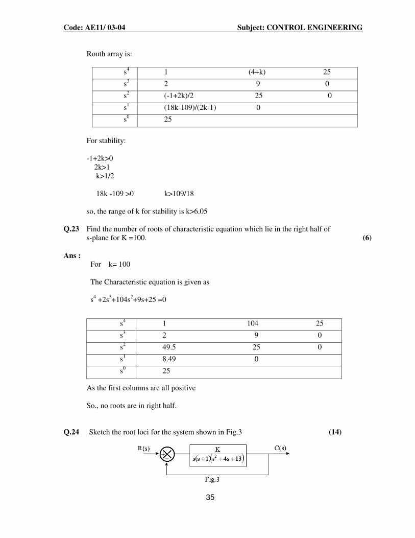
Q.23 Find the number of roots of characteristic equation which lie in the right half of s-plane for K =100. (6)
Ans : For k= 100 The Characteristic equation is given as s4 +2s3+104s2+9s+25 =0 As the first columns are all positive So., no roots are in right half.
Q.24 Sketch the root loci for the system shown in Fig.3 (14)
s4 1 104 25
s3 2 9 0
s2 49.5 25 0
s1 8.49 0
s0 25

Code: AE11/ 03-04 Subject: CONTROL ENGINEERING
36
Ans :
k G(s) = ---------------------- s(s+1)(s2+4s+13) Poles s=0, -1,-2±j3 n=4,m=0 ± 180(2q+1) angle of asymptotes = ----------------- = ±45, ±135 (n-m) -2-2-1 centroid = -------------- = -1.25 4 4 M(s) = ------------------------ (s2+s)(s2+4s+13)+k The Characteristic equation is given as s4+4s3+13s2+s3+4s2+13s+k = 0 k = -(s4+5s3+17s2+13s) dk/ds = -(4s3+15s2+34s+13) = 0 so, s= -0.4664, -1.6418±j2.067 so, the break away point is -0.4664 Angle of departures For complex poles
Ø1= 90, Ø2 = 180 – 1tan− (3/1), Ø3 = 180 – 1tan− (3/2) So., at A
= 180ο – (Ø1+ Ø2+ Ø3)
= -142.12ο
and A* = 142.12ο

Code: AE11/ 03-04 Subject: CONTROL ENGINEERING
37
Figure Root Locus
Q.25 The forward path transfer function of a Unity-feedback control system is given as
( )( )s5.01s1.01s
K)s(G
++=
Draw the Bode plot of G(s) and find the value of K so that the gain margin of the system is 20 dB. (14)
k Ans : G(s) = ----------------------- s(1+0.1s)(1+0.5s)
k G(jw) = ----------------------- jw(1+0.1jw)(1+0.5jw)
corner frequencies:2,10.
1 2 10 20 100
Magnitude db/dec
-20 -40 -60 -60 -60
phase -122.27 -146.3 -216 -238 -263
Code: AE11/ 03-04 Subject: CONTROL ENGINEERING
38
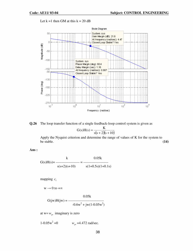
Let k =1 then GM at this k = 20 dB
Q.26 The loop transfer function of a single feedback-loop control system is given as
( )( )10s2ss
K)s(H)s(G
++=
Apply the Nyquist criterion and determine the range of values of K for the system to be stable. (14)
Ans :
k 0.05k G(s)H(s)= -------------------- = --------------------- s(s+2)(s+10) s(1+0.5s)(1+0.1s)
mapping 1c
w → 0 to +∞ 0.05k G(jw)H(jw) = ------------------------------ -0.6w2 + jw(1-0.05w2)
at w= pcw imaginary is zero
1-0.05w2 =0 pcw =4.472 rad/sec.

Code: AE11/ 03-04 Subject: CONTROL ENGINEERING
39
at pcw
GH = -.00417k
Mapping 2c
K
GH(s) = ------ = 0 3je
θ− at s= lim Rej Ө s3 R→ ∞ When
Ө = π /2 G(s)H(s) = 0 / 2ie
π−
Ө =- π /2 G(s)H(s) = 0 3 / 2ie
π+
Mapping 3c
W → - ∞ to 0
It is mirror image of 1c mapping
Mapping 4c
For s= lim Rej Ө R→0
Ө = - π /2 G(s)H(s) = ∞ / 2ie π+
Ө = π /2 G(s)H(s) = ∞ / 2ie
π−
FIGURE: NYQUIST PLOT
Range of values of k for the system to be stable. Limiting value of k

Code: AE11/ 03-04 Subject: CONTROL ENGINEERING
40
-0.00417k = -1 k = 240 So when k<240 , the closed loop system is stable.
Q.27
(a) The transfer functions for a single-loop non-unity-feedback control system are given as
1s
1 H(s) ,
2ss
1G(s)
2 +=
++=
Find the steady-state errors due to a unit-step input, a unit-ramp input and a
parabolic input. (b) Find also the impulse response of the system described in part (a). (5)
Ans :
(a) 1 1 G(s) = ---------------- H(s) = -------- s2 + s+2 (s+1)
R(s)
E(s) = ------------------ sse = lim sE(s)
1 + G(s)H(s) s→0 for unit step input s*1/s
sse = lim -----------------------------
s→0 1 + (1/s2+s+2)(1/s+1) 1 = ----------------------- = 2/3 1 +( ½) for unit ramp input
s*1/ 2s
sse = lim ------------------------ = ∞
s→0 1 + G(s)H(s) for unit parabolic input s*1/s3
sse = lim ------------------- = ∞
s→0 1 + G(s)H(s) C(s) G(S) 1/(s2 + s+2) ----- = --------------------- = --------------------------------- R(s) 1+ G(S)H(s) 1 + (1/s2+s+2)(1/s+1)

Code: AE11/ 03-04 Subject: CONTROL ENGINEERING
41
(s+1) = -------------------------------- (s2+s+2)(s+1)+1 (s+1) = ----------------------------- s3+2s2+3s+3 (b). Impulse response of the system:
Q.28 Derive the transfer function of the op amp circuit shown in Fig.3. Also, prove that the circuit processes the input signal by ‘proportional + derivative + integral’ action. (9)
Ans :
20 2 2 2 1 1
1 211
11
1 1 2 20 2 2 1
1 2 1 2 0
1( ) ( 1)( 1)
1( ) ( )
1
( )1( ) ( ) ( )
i
t
ii
RE s sc R c s R c s
E s R c sRsc
Rsc
de tR c R ce t e t e d R c
R c R c dtτ τ
++ +
= − = −
+
+= − − −∫
Q.29 The electro hydraulic position control system shown in Fig.4 positions a mass M
with negligible friction. Assume that the rate of oil flow in the power cylinder is

Code: AE11/ 03-04 Subject: CONTROL ENGINEERING
42
pKxKq 21 ∆−= where x is the displacement of the spool and p∆ is the differential
pressure across the power piston. Draw a block diagram of the system and obtain
therefrom the transfer function ( ) ( )sRsY .
The system constants are given below.
Mass M = 1000 kg Constants of the hydraulic actuator:
1K = 200 cm2/sec per cm of spool displacement
2K = 0.5 cm2/sec per gm- ω t/ cm2
Potentiometer sensitivity KP = 1 volt/cm Power amplifier gain KA = 500 mA/volt Linear transducer constant K = 0.1 cm/mA Piston area A = 100 cm2
(14)
Ans :
.
1 2
..
2
2
2
( )
( )
( ) 2
( ) 0.02 2
p A
k x A y k p
Ak p M y
k
r y k k k x
Y s
R s s s
− = ∆
∆ =
− =
=+ +

Code: AE11/ 03-04 Subject: CONTROL ENGINEERING
43
Q.30 A servo system is represented by the signal flow graph shown in Fig.5. The nominal
values of the parameters are 5K and 5K 1,K 321 === .
Determine the overall transfer function ( ) ( )sRsY and its sensitivity to changes in
1K under steady dc conditions, i.e., s = 0. (14)
Ans :
Fig: Signal flow graph
1 1( )( )
( )
PY sM s
R s
∆= =
∆
One forward path with gain 3 11 2 ( 1)
k kP
s s=
+
Three feedback loops with gains
11 2
1 221
3 131 2
5
( 1)
( 1)
( 1)
Ps s
k kP
s
k kP
s s
= −+
= −+
= −+
So,
3 11 2
2 2
51
( 1)( 1) ( 1)
k kk k
ss s s s
∆ = − − − −
++ +
1 1∆ = since all loops are touching.

Code: AE11/ 03-04 Subject: CONTROL ENGINEERING
44
1
1
1
2
1 1
2 2
1 1 1
2
1 1 1
01
5( )
( 1 5 ) 5 5
( 1 5 ) 5 5*
( 1 5 ) 5 5
5( ) 0.5
5 5
M
k
M
kw
kM s
s s k k
k s s k k sMS
k M s s k k
S jwk=
=+ + + +
+ + + −∂= =
∂ + + + +
= =+
Q.31 Determine the values of K>0 and a>0 so that the system shown in Fig.6 oscillates at
a frequency of 2 rad/sec. (10)
Ans :
3 2( ) (2 ) 1s s as k s k∆ = + + + + +
s3 1 (2+k) 0
s2 a 1+k 0
s1 (2+k)-(1+k)/a 0
s0 1+k
From the Routh’s array ;we find that for the system to oscillate (2+k)a = 1+k
Oscillation frequency = 1
2k
a
+=
These equations give a = 0.75 , k=2 Q.32 Consider the control system shown in Fig 7 in which a proportional compensator is
employed. A specification on the control system is that the steady-state error must be less than two per cent for constant inputs.
(i) Find Kc that satisfies this specification. (5)
(ii) If the steady-state criterion cannot be met with a proportional compensator, use
a dynamic compensator s
K3)s(D I+= . Find the range of IK that satisfies the
requirement on steady-state error. (9)
Code: AE11/ 03-04 Subject: CONTROL ENGINEERING
45
Ans : (i).
s3 1 5 0
s2 4 2+2Kc 0
s1 (18-2Kc)/4 0 0
s0 2+2Kc 0
The system is stable for Kc < 9.
Kp = 0lims −> D(s)G(s) = Kc; sse = 1/(1+Kc); sse = 0.1 (10 %) is the minimum
possible value for steady state error. Therefore sse less than 2 % is not possible
with proportional compensator.
(ii) Replace Kc by D(s) = 3 + Ki/s . The closed-loop system is stable for 0 < Ki <3. Any value in this range satisfies the static accuracy requirements.
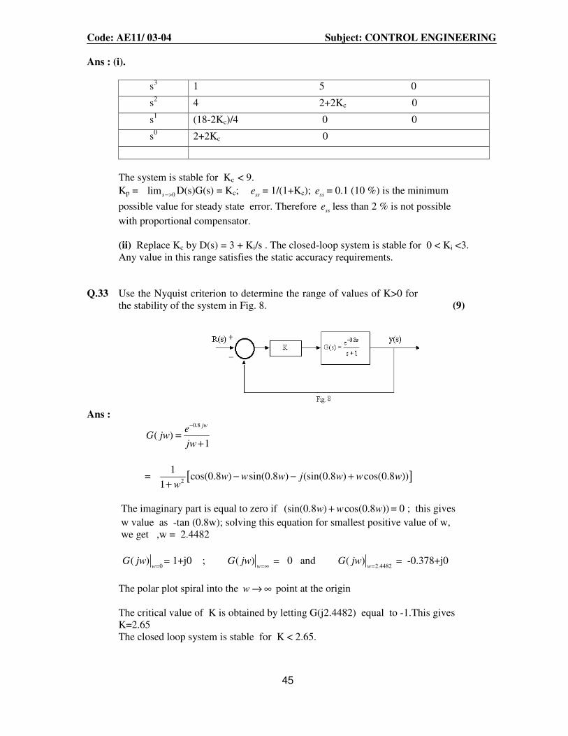
Q.33 Use the Nyquist criterion to determine the range of values of K>0 for the stability of the system in Fig. 8. (9)
Ans :
0.8
( )1
jwe
G jwjw
−
=+
= [ ]2
1cos(0.8 ) sin(0.8 ) (sin(0.8 ) cos(0.8 ))
1w w w j w w w
w− − +
+
The imaginary part is equal to zero if (sin(0.8 ) cos(0.8 ))w w w+ = 0 ; this gives
w value as -tan (0.8w); solving this equation for smallest positive value of w, we get ,w = 2.4482
0
( )w
G jw=
= 1+j0 ; ( )w
G jw=∞
= 0 and 2.4482
( )w
G jw=
= -0.378+j0
The polar plot spiral into the w → ∞ point at the origin The critical value of K is obtained by letting G(j2.4482) equal to -1.This gives K=2.65 The closed loop system is stable for K < 2.65.

Code: AE11/ 03-04 Subject: CONTROL ENGINEERING
46
Q.34 A unity-feedback system has open-loop transfer function )2s)(1s(s
4)s(G
++= .
(i) Using Bode plots of )j(G ω , determine the phase margin of the system.
(ii) How should the gain be adjusted so that phase margin is 50°? (iii)Determine the bandwidth of gain-compensated system. The –3dB contour of the Nichols chart may be constructed using the following table. (10)
Phase, degrees
0 -30 -60 -90 -120 -150 -180 -210
Magnitude, dB
7.66 6.8 4.18 0 -4.18 -6.8 -7.66 -6.8
Ans :
Bode Diagram
Frequency (rad/sec)
-150
-100
-50
0
50
100
Magnitu
de (
dB
)
System: d
Gain Margin (dB): 3.52
At frequency (rad/sec): 1.41
Closed Loop Stable? Yes
10-2
10-1
100
101
102
-270
-225
-180
-135
-90
Phase (
deg)
System: d
Phase Margin (deg): 11.4
Delay Margin (sec): 0.175
At frequency (rad/sec): 1.14
Closed Loop Stable? Yes
(i). From the bode plot we get PM = 11.4 deg (ii). For the phase margin of 50 deg , we require that mag(G(jw)H(jw)) =1 and ang(G(jw)H(jw)) = -130 deg , for some value of w ,from the phase curve of G(jw)H(jw) ,we find that ang(G(jw)H(jw)) = -130 deg at w = 0.5. The magnitude of G(jw)H(jw) at this frequency is approximately 3.5 .The gain must be reduced by a factor of 3.5 to achieve a phase margin of 50 deg . (iii).On a linear scale graph sheet , dB Vs phase curve of open loop frequency response is plotted with data coming from bode plot .On the same graph sheet ,the -3 dB contour using the given data is plotted . The intersection of the curves occurs at w = 0.911 rad
/

Code: AE11/ 03-04 Subject: CONTROL ENGINEERING
47
sec . Therefore band width Wb = 0.911 (Nichols chart is not required).
-250 -200 -150 -100 -50 0-8
-6
-4
-2
0
2
4
6
8
Q.35 Discretize the PID controller
( ) ( ) ( )
+τ+= ∫
t
0 DI
Cdt
tdeTdte
T
1teK)t(u to obtain PID algorithm in
(i) position form (ii) velocity form.
What are the advantages of velocity PID algorithm over the position algorithm?
Ans :
The PID controller can be written as
0
1 ( )( ) ( ) ( )
t
c D
I
de tu t K e t e t dt T
T dt
= + +
∫
It can be realized as
( ) ( ) ( ) ( )p I Du k u k u k u k= + +
Position PID algorithm:
( ) ( )p cu k K e k=
If the S(k-1) approximates the area under the e(t) curve up to t = (k-1)T, Then the approximation to the area under the e(t) curve up to t = kT is given by S(k)=S(k-1)+Te(k)
( ) ( )c
I
I
Ku k S k
T=
[ ]( ) ( ) ( 1)c DD
K Tu k e k e k
T= − −

Code: AE11/ 03-04 Subject: CONTROL ENGINEERING
48
Velocity PID Algorithm :
The PID algorithm can be realized by following equation.
[ ]( ) ( ) ( ) ( ) ( 1)c c D
c
I
K K Tu k K e k S k e k e k
T T= + + − −
[ ]( 1) ( 1) ( 1) ( 1) ( 2)c c Dc
I
K K Tu k K e k S k e k e k
T T− = − + − + − − −
subtracting above two equations
[ ]( ) ( 1) ( ) ( 1) ( ) ( ) 2 ( 1) ( 2)Dc
I I
TTu k u k K e k e k e k e k e k e k
T T
− − = − − + + − − + −
Now only the current change in the control variable ( ) ( ) ( 1)u k u k u k∆ = − − is calculated.
Compared to ‘position form’, the ‘velocity form’ provides a more efficient way to program the PID algorithm from the standpoints of handling the initialization when controller switched from ‘manual’ to ‘automatic’, and of limiting the controller output to prevent reset wind-up. Practical implementation of this algorithm includes the features of avoiding derivative kicks/filtering measurement noise.
Q.36 The open-loop transfer function of a control system is
)s1.01)(s5.01(s
10)s(H)s(G
++=
(i) Draw the Bode plot and determine the gain crossover frequency, and phase and gain margins.
(ii) A lead compensator with transfer function
s023.01
s23.01)s(D
+
+=
is now inserted in the forward path. Determine the new gain crossover frequency, phase margin and gain margin. (6+8)
Ans : (i)

Code: AE11/ 03-04 Subject: CONTROL ENGINEERING
49
From the bode plot of G(jw)H(jw) ; we find that wg= 4.08 rad/sec:
PM = 3.9 deg ; GM = 1.6 dB
(ii)
Bode Diagram
Frequency (rad/sec)
-150
-100
-50
0
50
System: r
Gain Margin (dB): 18.3
At frequency (rad/sec): 17.7
Closed Loop Stable? YesMag
nitu
de (
dB
)
10-1
100
101
102
103
-270
-225
-180
-135
-90
Pha
se (
deg)
System: r
Phase Margin (deg): 37.6
Delay Margin (sec): 0.131
At frequency (rad/sec): 5.02
Closed Loop Stable? Yes
From the new bode plot ,we find that Wg = 5 rad/sec ; PM = 37.6 deg ; GM = 18 dB, The increase in phase margin and gain margin implies that lead
compensation increases margin of stability .The increase in Wg implies that lead compensation increases the speed of response.

Code: AE11/ 03-04 Subject: CONTROL ENGINEERING
50
PART – III
DESCRIPTIVES
Q.1 A typical temperature control system for the continuously stirred tank is given in
Fig.6. The notations are θ for temperature, q for liquid flow and stF for the steam
supplied to the steam coil. Draw the block diagram of the system. (10)
Ans :
Q.2 Considering a typical feedback control system, give the advantages of a P+I controller as compared to a purely proportional controller. (4)
Ans :
P + I controller as compared to a purely proportional controller : If the controller is based on proportional logic, then in the new steady state, a non zero
error sse must exist to get a non zero value of control signal ssU . The operator must then
reset the set point to bring the output to the desired value. We need a controller that automatically brings the output to the set point which is done by PI, which gives a
steady control signal with system error sse = 0.

Code: AE11/ 03-04 Subject: CONTROL ENGINEERING
51
Q.3 Explain the procedure to be followed when in the Routh’s array all the elements of a
row corresponding to 4S are zeros. (4)
Ans : When all the elements of a row corresponding to s4 are zeros, then write the auxiliary equation. This is an equation formed by the coefficients of the row just above the row having all zeros. Here it means make an equation from the row corresponding to s5. Differentiate this equation and replace the entries in Routh’s array by the coefficients of this differential equation. Then follow the usual procedure.
Q.4 Justify the following statements :
(i) The impulse response of the standard second order system can be obtained from its unit step response.
(ii) The Bode plot of the standard second order function 2nn
2
2n
ωsω2s
ω
+ζ+ has a
high frequency slope of 40 db / decade. (iii) The two phase a.c. servomotor has an inherent braking effect under zero-
control-voltage condition. (iv) An L.V.D.T. can be used for measuring the density of milk. (4x3.5)
Ans :
(i) The impulse response of the standard second order system can be obtained from its unit step response by integrating it.
(ii) nw2
----------------------
s2 + 2ξ nw s + nw2
put s = jw 1 ---------------------------
1 + j(2ξ nw ) w – w2/ nw
2
let w/nw = u (normalized frequency)
1 = ----------------- 1 + j2ξu –u2 dB = 20 log ( 1/(1-u2 + j2ξu)) At low frequency such that u<<1 magnitude may be approximately dB = -20 log 1 = 0 For high frequency such that u>>1 the mag may be approximately dB = -20 log(u2)= -40log u Therefore an approximately mag plot for T.F consists of two straight line asymptotes, one horizontal line at 0 dB for u<=1and other line with a slope -40dB/dec for u>=1.

Code: AE11/ 03-04 Subject: CONTROL ENGINEERING
52
(iii)
In two phase AC servo motor there are two supplies. One with constant voltage supply to the reference phase and second one is control phase voltage which is given through servo amplifier. Torque speed characteristics
All these curves have –ve slope and these always depends on control voltage. Note that the curve for zero control voltage goes through the origin and the motor develops a decelerating torque which means braking.
Q.5 Write notes on any TWO of the following:
(i) Disturbance rejection. (ii) Turning method based on the process reaction curve. (iii) Phase lag compensation. (2 x 7)
Ans :
(i) Disturbance rejection :
The degree of disturbance rejection may be expressed by the ratio of ydG Gyd
(the closed loop transfer function between the disturbance d and the output y ) and pG
(the feed forward transfer function between the disturbance d and the output y) or

Code: AE11/ 03-04 Subject: CONTROL ENGINEERING
53
1
1
1
yd
d
p c p
GS
G G G= =
+
To improve the disturbance rejection, make dS small over a wide frequency range
(ii) Phase lag compensator:
It has a pole at -1/ βτ and a zero and -1/τ with zero located to the left of pole on the negative real axis. (s + 1/τ )
cG (s) = -------------
(s + 1/βτ )
oE (s) R2 + 1/sC
------- = ---------------------
iE (s) R1 + R2 + 1/sC
τ = R2C β = (R1 + R2)/R

Code: AE11/ 03-04 Subject: CONTROL ENGINEERING
54
Q.6 Compare the response of a P+D controller with that of a purely proportional
controller with unit step input, the system being a type–1 one. (6)
Ans :
k G(s) = ------------------ Let us consider a type 1 system s(s+a) If considering only proportional controller we can be able to improve the gain of the system. The steady state error due to step commands can theoretically be eliminated from proportional control systems by intentionally misadjusting the input value. By increasing the loop gain the following behavior exists. 1. Steady state tracking accuracy. 2 Disturbance rejection 3. Relative stability. i.e. rate of decay of the transients. All aspects of system behavior are improved by high gain proportional. By P.D. controller: We can able to improve the steady state accuracy using a P.D. controller, improvement of relative stability. The speed of response is also very fast using this type of controller.
Q.7 Write short notes on the following: (7+7)
(i) Controller tuning (ii) Phase-lead compensation
Ans :
(i) Controller tuning
Considering the basic control configuration, wherein the controller input is the error between the desired output and the actual output.

Code: AE11/ 03-04 Subject: CONTROL ENGINEERING
55
METHOD 1. This method is applicable only if dynamic model of plant is not available and step response of the plant is S-shaped curve .Then tuning done by Zeigler –Nichols method. Procedure: Obtaining the step response, from that find the dead time (L) and time constant (T) Then the values of controller is given by
Proportional gain ( pK ) =1.2(T/L)
Integral time constant =2L Derivative time constant=0.5L Note: There are no specific tuning method available if plant model is not known and step response is not S-shaped curve. METHOD 2. This method is applicable only if dynamic model of plant is known and no integral term in the transfer function. Procedure: Find the critical gain (K) and critical time period (T) at which the system is oscillating using routh array or root locus. Then the controller parameters are given by Proportional gain = 0.6 K Integral time constant=0.5 T Derivative time constant= 0.125 T METHOD 3. This method is applicable only dynamic model of the plant, having an integral term in the transfer function. If the critical period and the gain cannot be calculated, then tuning is done through root locus method.
(ii) Phase lag compensator
Consider the following circuit. This circuit
Has the following transfer function Eo T2 ( 1 + T 1 s) ----------- = -------------------------- (1) E1 T1 ( 1 + T 2 s)

Code: AE11/ 03-04 Subject: CONTROL ENGINEERING
56
Where T1 = R1 C1 and T2 = R2/ (R1 + R2) T1.
Obviously T1 > T2. For getting the frequency response of the network, but s = jw i.e.,
2 2
o 2 1
2 2
i 1 2
E T 1
E T 1
w T
w T
+=
+ (2)
And phase ф = tan-1 wT1 - tan-1 wT2
Let us consider the polar plot for this transfer function as shown in figure below. We can observe that at low frequencies, the magnitude is reduced being T2 / T1 at w=0.
Next, let us consider the bode plot the transfer function as shown in figures below.
We observe here that phase ф is always positive. From magnitude plot we observe that transfer function has zero db magnitude at w= 1 / T2 . We can put dф / dw =0 to get maximum value of ф which occurs at some frequency wm
Code: AE11/ 03-04 Subject: CONTROL ENGINEERING
57
i.e., wm = 1 / ( 1 2T / T )
фmax = tan-1 [ T1 / T2 ]1/2 - tan-1 [ T2 / T1 ]
1/2 In this network we have an attenuation of T2 / T1 therefore, we can use an amplification of T1 / T2 to nullify the effect of attenuation in the phase network.
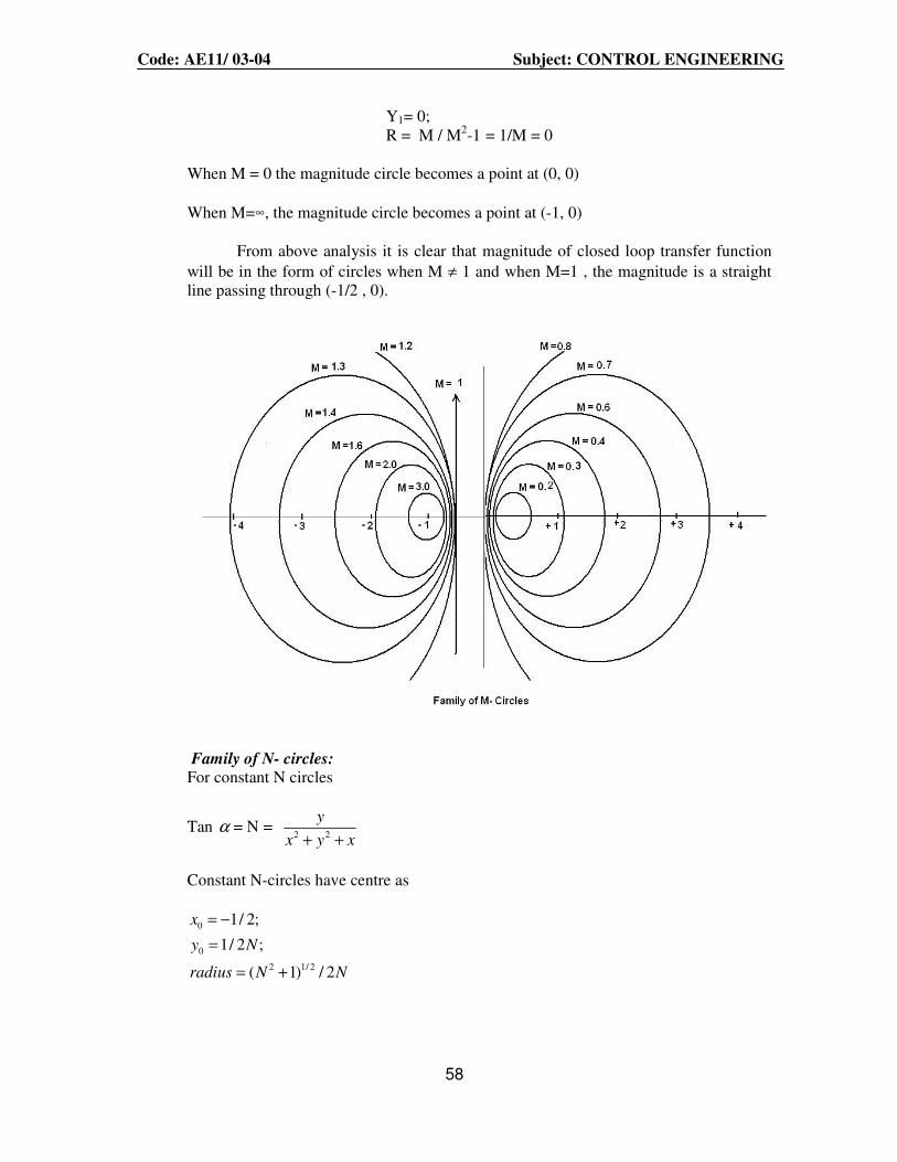
Q.8 Write short notes on the following : (i) Constant M and N circles. (ii) Stepper Motor. (2 x 7 = 14)
Ans.
(i) Constant M and N circles:
The magnitude of closed loop transfer function with unity feedback can be
shown to be in the form of circle for every value of M. These circles are called M-circles. If the phase of closed loop transfer function with unity feedback is α, then it can be shown that tan α will be on the form of circle for every value of α. These circles are called N- circles. The M and N circles are used to find the closed loop frequency response graphically form the open loop frequency response G(jw) without calculating the magnitude and phase of the closed loop transfer for at each frequency . For M circles: Consider the closed loop transfer function of unity feedback system. C(s) / R(s) = G(s) / 1+G(s) Put s = jw; C(jw) /R(jw) =G(jw) / 1 + G(jw) ( X + M2 / M2-1 )2 + γ2 = ( M2 / M2-1 )2 ---- (1)
The equation of circle with centre at (X1,Y1) and radius r is given by ( X - X1)
2 + (Y – Y1 )2 = r2 -----(2)
On comparing eqn (1) and (2) When M = 0; X1 = - M2 / M2-1 =0 Y1 = 0 R = M / M2-1 = 0;
When M = ∞ X1 = - M2 / M2-1 = -1
Code: AE11/ 03-04 Subject: CONTROL ENGINEERING
58
Y1= 0; R = M / M2-1 = 1/M = 0 When M = 0 the magnitude circle becomes a point at (0, 0)
When M=∞, the magnitude circle becomes a point at (-1, 0)
From above analysis it is clear that magnitude of closed loop transfer function
will be in the form of circles when M ≠ 1 and when M=1 , the magnitude is a straight line passing through (-1/2 , 0).
Family of N- circles: For constant N circles
Tan α = N = 2 2
y
x y x+ +
Constant N-circles have centre as
0
0
2 1/ 2
1/ 2;
1/ 2 ;
( 1) / 2
x
y N
radius N N
= −
=
= +

Code: AE11/ 03-04 Subject: CONTROL ENGINEERING
59
Family of N- circles
(ii) Stepper Motor:
A stepper motor transforms electrical pulses into equal increments of shaft motion called steps. It has a wound stator and a non-excited rotor. They are classified as variable reluctance, permanent magnet or hybrid, depending on the type of rotor. The no of teeth or poles on the rotor and the no of poles on the stator determine the size of the step (called step angle). The step angle is equal to 360 divided by no of step per revolution.
Operating Principle:
Consider a stepper motor having 4-pole stator with 2-phase windings. Let the rotor be made of permanent motor with 2 poles. The stator poles are marked A, B, C and D and they excited with pulses supplied by power transistors. The power transistors are switched by digital controllers a computer. Each control pulse applied by the switching device causes a stepped variation of the magnitude and polarity of voltage fed to the control windings.

Code: AE11/ 03-04 Subject: CONTROL ENGINEERING
60
Stepper motors are used in computer peripherals, X-Y plotters, scientific instruments, robots, in machine tools and in quartz-crystal watches.
Q.9 Define the transfer function of a linear time-invariant system in terms of its differential equation model. What is the characteristic equation of the system? (5)
Ans :
The input- relation of a linear time invariant system is described by the following nth-order differential output equation with constant real coefficients:
1 1
1 1 0 1 1 01 1
( ) ( ) ( ) ( ) ( ) ( )..... ( ) ..... ( )
n n m m
n nn n m m
d y t d y t dy t d u t d u t du ta a a y t b b b u t
dt dtdt dt dt dt
− −
− −− −+ + + + = + + + +
“Transfer function is defined as the ratio of Laplace transform of output variable to the input variable assuming all initial condition to be zero.”i.e. T(s)=Y(s)/U(s)=sm+bn-1s
m-1+ …………………..+b0/sn+an-1s
n-1+…….+a0
The characteristic equation is given by
1
1 1 0...... 0n n
ns a s a s a−
−+ + + + =
Q.10 Define the terms: (i) bounded-input, bounded-output (BIBO) stability, (ii) asymptotic stability. (2+2)
Ans :
(i) Bounded Input Bounded Stability :With zero initial conditions, the system is said to be bounded input bonded output (BIBO) stable, if its output y(t) is bounded to a bounded input u(t).

Code: AE11/ 03-04 Subject: CONTROL ENGINEERING
61
(ii) Asymptotic Stability : A linear time-invariant system is asymptotically stable if
for any set of finite ( )
0( )ky t ,there exists a positive number M,which depends on
( )
0( )ky t , such that
( )
( ) 0limt
y t M
y t→∞
≤ < ∞
=
Q.11 Discuss the compensation characteristics of cascade PI and PD compensators using
root locus plots. Show that (i) PD compensation is suitable for systems having unsatisfactory transient
response, and it provides a limited improvement in steady-state performance. (ii) PI compensation is suitable for systems with satisfactory transient response but
unsatisfactory steady-state response. (7+7)
Ans. PI Compensation : When a PI compensator is used in cascade, it increases the type of the system. With the root loci, we can see that steady state error is reduced once the type of the original system is increased. No satisfactory improvement in the transient performance is noted.
( ) ( ) ( ) ( )
( ) /
PI
PI P I
D s G s G s H s
G s K K s
=
= +
1/
1/
1/1
ss v
ss a
ss p
e k
e k
e k
=
=
= +
kp ,kv and ka values increase with the type of the system. PD Compensation: When a PD compensator is used in cascade (forward path),it results in the addition of an open loop zero in the original system.. Since addition of open loop zeros results in the leftward movement of the root loci, this effectively means the increase in the value of the damping ratio which improves the transient response but no satisfactory improvement in the steady state response is seen
( ) ( ) ( ) ( )
( )
PD
PD P D
D s G s G s H s
G s K K s
=
= +
' 2 / nk wξ ξ= +
Q.12 State and explain the Nyquist stability criterion. (5) Ans :
If the contour of the open-loop transfer function G(s)H(s) corresponding to the Nyquist contour in the s-plane encircles the point (-1 +j0) in the counterclockwise direction as many times as the number of right half s-plane poles of G(s)H(s),the closed-loop system is stable. In the commonly occurring case of the open-loop stable system ,the closed-loop system is stable if the counter of G(s)H(s) does not encircle (-1 +j0) point, i.e., the net encirclement is zero.

Code: AE11/ 03-04 Subject: CONTROL ENGINEERING
62
Q.13 When is a control system said to be robust? (4)
Ans :
A control system is said to be robust when (i) It has low sensitivities (ii) It is stable over a wide range of parameter variations; and (iii) The performance stays within prescribed (but practical) limit bounds in presence of changes in the parameters of the controlled system and disturbance input.