Adverse Selection in Credit Markets:Evidence from a Policy Experiment

August 2007

Stefan Klonner, Cornell University

Ashok S. Rai, Williams College

Abstract: We test if riskier borrowers are willing to pay higher interest rates than safer

borrowers are as predicted by Stiglitz and Weiss (1981). The data are from an Indian

�nancial institution where interest rates are determined by competitive bidding. The

government imposed an interest rate ceiling in 1993 and then relaxed the ceiling in 2002:

Changes in default patterns are analyzed before and after each of these policy changes. We

�nd evidence of adverse selection despite the use of collateral as a screening device. This

study isolates adverse selection from moral hazard and controls for information on riskiness

observed by the lender but not by the researcher.

JEL Codes: D82, G21, O16

Keywords: Defaults, Risk, Auctions, Asymmetric Information.

0We thank Garance Gennicot, Bill Gentry, Magnus Hattlebak, Seema Jayachan, Dean Karlan, Ted

Miguel, Rohini Pande, Antoinette Schoar and Jonathan Zinman for useful suggestions. We also thank

seminar/conference participants at Berkeley, Boston University, Cornell, EUI Florence Credit Contracts

Conference, Groningen Micro�nance Conference, Harvard-MIT, Indian School of Business, Montreal CIR-

PEE Conference, NEUDC, Paris-Jourdan, Toulouse, Wharton Indian Financial System conference, and

Williams for comments. We are grateful to the South Indian Chit Fund company for sharing their data and

their time. All errors are our own. Klonner: Dept. of Economics, Cornell University, 444 Uris Hall, Ithaca,

NY 14853 stefan@klonner.de; Rai: Dept. of Economics, Fernald House, Williams College, Williamstown,

MA 01267 arai@williams.edu

1

1 Introduction

Many economists believe that asymmetric information impedes the e¢ cient functioning of

markets. Even though there is substantial theoretical research assuming asymmetric infor-

mation, the empirical evidence is rather mixed and largely con�ned to insurance markets

(Chiappori and Salanie 2003). In this paper we look for evidence of adverse selection in

credit markets. We test if riskier borrowers are willing to pay higher interest rates than

safer borrowers are. This well-known prediction of Stiglitz and Weiss�(1981) adverse se-

lection model has had considerable in�uence in �nance, development and macroeconomics

but has received little empirical scrutiny.

There are three main empirical challenges for such a study. First, the lender may

have "soft" information on borrower riskiness which by de�nition is di¢ cult to transmit or

codify (Berger and Udell, 1995;Petersen and Rajan 1994; Uzzi and Lancaster, 2003). A

researcher who is uninformed about the lender�s soft information may erroneously conclude

that there is adverse selection on unobserved riskiness. Secondly, lenders often require

collateral. Even if adverse selection is an underlying friction in credit markets, the lender

may be able to mitigate adverse selection through collateral requirements (Bester 1985) or

using cosigners as collateral (Besanko and Thakor 1987). Finally, researchers only have

information on defaults. It is entirely possible that higher interest rates increase default

rates for moral hazard reasons instead of adverse selection. It is di¢ cult empirically to

distinguish between the two.

The contribution of this paper is to address all three empirical challenges. We dis-

tinguish unobserved riskiness from riskiness that is observed by the lender but not by the

researcher, we allow for the e¤ects of collateral, and we disentangle adverse selection from

moral hazard. We �nd robust evidence of adverse selection � privately informed risky

borrowers are willing to pay higher interest rates than privately informed safer borrowers

are despite collateral requirements in place to deter them.

Our paper contributes to an empirical literature on adverse selection. This includes tests

for adverse selection in used car markets (Genesove 1993), annuity markets (Finkelstein and

2

Poterba, 2004) and most speci�cally, in credit markets (Ausubel 1999; Karlan and Zinman,

2007). We use a natural experiment involving a South Indian �nancial institution; Ausubel

(1993) and Karlan and Zinman (2007) use randomized �eld experiments. We are able to

isolate adverse selection from moral hazard, while Ausubel (1999) is not able to do so. We

�nd much stronger evidence of adverse selection than Karlan and Zinman (2007) do. A

�nal di¤erence is that both Ausubel (1999) and Karlan and Zinman (2007) use data from

uncollateralized lenders. So unlike us they cannot test whether adverse selection persists

in the presence of collateral.

The �nancial arrangements we study are Roscas (or Rotating Savings and Credit Asso-

ciations). These are popular in many developing countries. In a Rosca, a group of people

get together regularly, each contributes a �xed amount, and at each meeting one of the

participants receives the collected pot. In random Roscas, the pot is awarded in each

round by lottery. In bidding Roscas, the subject of our study, the pot is awarded to the

highest bidder.1 Once a participant has received a pot he is ineligible to bid for another.

Such a participant may default (stop making contributions) after receiving the pot. Unlike

textbook �nancial markets, every participant in a bidding Rosca receives loans of di¤erent

sizes and durations and at di¤erent interest rates.

We test if riskiness is positively related to the willingness to pay by exploiting an ex-

ogenous policy shock. In September 1993; the government unexpectedly imposed a bid

ceiling (of 30% of the total pot). This ceiling typically binds in early rounds of bidding

Roscas transforming them into random Roscas since many participants bid up to the ceiling

but only one of them chosen by lottery receives the pot. To test for self selection based

on unobserved riskiness, we compare the riskiness pro�le of borrowers before and after the

policy shock. Riskier borrowers who have a higher willingness to pay can simply outbid

the others and take early pots in the absence of the ceiling. But the ceiling e¤ectively ties

their hands. Even though safer borrowers have lower willingness to pay for early pots, they

1The rationale for random and bidding Roscas has been examined by Anderson and Baland (2002),

Besley, Coate and Loury (1993), Calomiris and Rajaraman (1998), Klonner (2003, 2006) and Kovsted and

Lyk-Jensen (1999), among others.

3

may still win early pots because of the lottery introduced by the ceiling. Riskier borrowers

are hence pushed back to later pots. In other words. the bid ceiling causes a �attening of

the riskiness pro�le of borrowers. This is easiest to see in an extreme case: suppose the

bid ceiling were set at zero percent transforming the bidding Rosca into a purely random

Rosca. The average riskiness of all borrowers would be the same implying a completely

�at risk pro�le.

We use a di¤erence-in-di¤erence speci�cation to capture this �attening. We predict

that the di¤erence between the riskiness of early and late borrowers is smaller after the policy

shock compared with before if there is self selection based on riskiness but is una¤ected if

there is no such self selection. Borrower riskiness is unobserved, however; only default

rates are observed. We �nd that defaults are indeed �atter as a result of the policy shock

exactly as predicted by selection. But default rates could be �atter for reasons completely

unrelated to selection including (a) di¤erences in riskiness observed by the lender but not

necessarily by the researcher (b) moral hazard (c) changes in the composition of Rosca

participants and (d) transitory aggregate shocks.

We address all four alternative explanations for the �attening of default rates. We

need to isolate the privately observed from the publicly observed component of riskiness

to address concern (a) since we are interested in selection on the former and not on the

latter. We do so by controlling for the collateral required of borrowers since collateral

requirements have been shown to be based on observed riskiness (Berger and Udell 1995;

Jimenez, Salas and Saurina 2006; Liberti and Mian 2006). Since loan terms become more

favorable to early borrowers relative to late as a result of the ceiling, moral hazard could

cause the �attening of observed defaults (concern b). So we control for loan terms while

taking the double di¤erence in defaults to isolate adverse selection from moral hazard. We

address concern (c) by showing how our di¤erence-in-di¤erence test remains consistent even

if changes in the average riskiness of the pool of participants alone caused the �attening of

default rates We exploit the overlaps in the Roscas started before and after the policy

shock to address concern (d). In all four cases we show how our estimator based on the

4

conditional double di¤erence in observed defaults consistently captures the double di¤erence

in unobserved riskiness.

We �nd that borrowers willing to pay higher interest rates are riskier than those who

are not despite the use of collateral requirements. The �attening of defaults caused by self

selection on unobserved riskiness is substantial. Our estimates suggest that defaults of early

borrowers fell by one-�fth and defaults of later borrowers rose by one-�fth as a consequence

of the bid ceiling.. We reject the null hypothesis of no self selection on unobserved riskiness.

This result is remarkably robust to alternative speci�cations of the di¤erence-in-di¤erence

test and to controls for observed riskiness, moral hazard and aggregate shocks.

We also examine the e¤ect of a partial relaxation of the bid ceiling in 2002 on arrears

(overdues at the end of the loan term). We �nd that the 2002 reversal had the opposite

e¤ect on arrears. Riskier participants could get their hands on early pots more easily after

2002 and so observed arrear pro�les became steeper. In sum, exogenously capping interest

rates in 1993 �attened the default pro�le while relaxing the cap in 2002 made the arrear

pro�le steeper exactly as predicted.

Financial constraints on development are a major academic and policy concern (Ar-

mendariz and Morduch, 2005; Banerjee 2003). Our results provide evidence of a speci�c

impediment to �nancial access in developing countries. The bidding Roscas we study

are not small scale and personalized (as in Anderson, Baland and Moene 2004): Instead,

a commercial organizer arranges �nancial intermediation between Rosca participants who

have no social ties. The organizer takes on the default risk and receives a commission

in exchange. It is the Rosca organizer who imposes a collateral requirement (asks for

cosigners with regular salaries) on the winners of the pot based on how risky he perceives

them to be. Cosigners also potentially serve as a deterrent for unobserved riskiness, but we

�nd that they are ine¤ective in doing so.

Finally we brie�y clarify what we do not do in this paper.

1. We test for a speci�c information asymmetry: Do borrowers have private information

on their own riskiness (or equivalently, dishonesty) that the Rosca organizer? There

5

may of course be other unobserved characteristics on which borrowers di¤er such as

impatience or productivity that have nothing to do with riskiness but a¤ect a bor-

rower�s willingness to pay for an early pot. We do not test for asymmetric information

on those dimensions.

2. We �nd evidence that the bid ceiling does reduce self selection on unobserved riskiness.

We follow Stiglitz and Weiss (1981) in referring to such self selection on riskiness as

"adverse" but we make no claims about whether such self selection (or the bid ceiling

that prevents self selection) has positive or negative welfare e¤ects in bidding Roscas.2

Just as Ausubel (1999) and Karlan and Zinman (2007) therefore, we use the term

adverse selection throughout this paper to refer to the positive relationship between

willingness to pay and unobserved riskiness, not to the welfare loss relative to a full

information environment.

3. We do not claim either the presence or absence of moral hazard. At �rst glance it

might seem that the lottery introduced by the bid ceiling could be used to isolate

moral hazard. However identifying moral hazard in this way is impossible since only

the identity of the lottery winner but not of all lottery entrants is recorded.

Paper Outline

We motivate our empirical strategy in section 2. We provide additional background on

bidding Roscas in South India, and on the policy shock in section 3. We construct a

simple model of bidding Roscas when riskiness is unobserved in section 4. We discuss our

identi�cation strategy in section 5. We discuss our main results from the 1993 policy shock

in section 6. We examine a reverse policy shock in 2002 as a robustness check in section

2 In contrast with equilibrium credit rationing in Stiglitz and Weiss (1981), credit rationing was exoge-

nously imposed here. While the bid ceiling constrained riskier borrowers, it also reduced participation in

Roscas which was undesirable from the Rosca organizer�s perspective. Presumably if the gains outweighed

the costs of imposing a bid ceiling, the Rosca organizer would have imposed it voluntarily in the absence of

any government intervention.

6

7. We conclude in section 8.

2 Motivating Examples

In this Section we introduce the rules of bidding Roscas before and after the 1993 policy

shock. We describe our empirical strategy for distinguishing adverse selection (on unob-

served risk) from selection on observed risk and from moral hazard. We do so through

some stylized examples. This section is intended to be an intuitive non-comprehensive

introduction to several issues that will taken up more carefully later in the paper.

Unrestricted and Restricted Roscas

Bidding Roscas match borrowers and savers. Each month participants contribute a �xed

amount to a pot. They then bid to receive the pot in an oral ascending bid auction where

previous winners are not eligible to bid. The highest bidder receives the pot of money less

the winning bid and the winning bid is distributed among all the members as a dividend.

Consequently, higher winning bids mean higher interest payouts to later recipients of the

pot. Over time, the winning bid typically falls as the duration for which the loan is taken

diminishes.

To illustrate these rules, consider a 3 person Rosca which meets once a month and each

participant contributes $10: Suppose the winning bid is $12 in the �rst month. Each

participant receives a dividend of $4: The recipient of the �rst pot e¤ectively has a net

gain of $12 (i.e. the pot less the bid plus the dividend less the contribution). Suppose that

in the second month (when there are 2 eligible bidders) the winning bid is $6: And in the

�nal month, there is only one eligible bidder and so the winning bid is 0:

We shall refer to the �rst recipient as the early borrower in what follows. The second

recipient saves $6 , then borrows $16 and �nally repays $10: Since we focus on the risk of

defaulting contributions owed subsequent to winning the pot in this paper, we will refer to

the second recipient as the late borrower in what follows. The net gains and contributions

7

in this Rosca with unrestricted bidding are:

Example U

Month 1 2 3

Winning bid 12 6 0

Early Borrower 12 -8 -10

Late Borrower -6 16 -10

Saver -6 -8 20

The early recipient receives $12 and repays $8 and $10 in subsequent months (which implies

a 43% monthly interest rate). The �nal recipient is a pure saver: she saves $6 for 2 months

and $8 for a month and receives $20 (which implies a 25% monthly rate). Notice that an

unrestricted bidding Rosca allows participants to self select �a participant with a higher

willingness to pay can outbid another.

Next we discuss an example where bidding is restricted by the policy change. The bid

ceiling is 30% of the pot (or $9): In the �rst month, suppose that two participants are

willing to pay more than $9: Since bidding stops at the ceiling, one of the two is chosen by

lottery to receive the pot. The early recipient contributes $10, receives the pot less the

bid, $21; and also receives a dividend of $3; which provides a net gain of $14 in the �rst

month. Each of the other participants contributes $10 and receives a dividend of $3 in the

�rst month. So the payo¤s in this Rosca with restricted bidding are:

Example R

Month 1 2 3

Winning bid 9 6 0

Early Borrower 14 -8 -10

Late Borrower -7 16 -10

Saver -7 -8 20

The ceiling substantially lowers the interest rate on borrowing for the early borrower (and

8

also the interest rate on savings for the saver). Further, the ceiling makes it di¢ cult for

participants to self select.

Empirical Approach

In example U; the early borrower has demonstrated a higher willingness to pay for the �rst

pot than the late borrower has for the �rst pot. If participants di¤er in their inherent

riskiness, then a riskier participant will be be willing to pay more for the �rst pot than a

safer participant. This is an implication of adverse selection analogous to Stiglitz and Weiss

(1981). So riskier participants will all else equal choose early pots and safer participants

will choose later pots. It is possible that self selection in Roscas is based only on other

characteristics (e.g. impatience or productivity) but participants are all equally risky. In

such a case, the early borrower would be no riskier than the late borrower. There would be

no self selection on riskiness.

Riskiness is unobserved by the researcher however. We do have data on default rates,

i.e. on whether contributions have been made subsequent to receipt of the pot. The

empirical challenge is to infer whether there are di¤erences in unobserved riskiness driving

self selection in Roscas when we just have data on di¤erences in observed defaults.

Consider �rst a naive empirical approach: simply taking the di¤erence between indi-

vidual default rates of early and late borrowers in example U . Adverse selection would

imply that early borrowers have higher default rates than late borrowers. But even if early

and late borrowers were inherently equally risky, there could be several other explanations

for this di¤erence in defaults. For instance, the early borrower has to make contributions

at dates 2 and 3 while the late borrower has contributions due only at date 3: Assume

that the �rst contribution after receiving a pot is easier to make than the second. So for

this purely mechanical reason the early borrower may have a higher default rate than the

late borrower. Taking the di¤erence in defaults between early and late borrowers does not

isolate adverse selection.

The restricted Rosca (example R) provides an opportunity to investigate default pat-

9

terns when self selection is hampered. Consider another empirical approach: di¤erence in

di¤erences. If there were adverse selection, riskier participants should win early pots before

the ceiling but may not after the ceiling. For instance, the early borrower in example U

has clearly demonstrated his willingness to pay more for the �rst pot than the late borrower

has. So the early borrower will all else equal be riskier than the late borrower in example

U: But in example R; it is conceivable that the early borrower has a lower willingness to

pay for the �rst pot than the late borrower�s willingness to pay for the �rst pot. In such a

situation, the late borrower may be riskier than the early borrower. In other words, the bid

ceiling may impede self selection on riskiness by changing the order of receipt of the pot.

We would then expect to see a �attening in the default pro�le as we move from Example

U to Example R: In other words, the di¤erence between default rates of early and late

borrowers should be higher in Example U than in Example R: But even if early and late

borrowers were inherently equally risky, there could be several alternative explanations for

a �attening of the default pro�le. For instance, the early borrower has more favorable

loan terms in the restricted Rosca relative to the early borrower in the unrestricted Rosca.

So moral hazard too would imply a �attening of default rates as a consequence of the bid

ceiling.

Suppose that there were many three person Roscas all with a $10 contributions both

before and after the ceiling was imposed. The participants in these Roscas may di¤er not

just in their riskiness but in other characteristics (such as impatience, productivity shocks

or urgency of consumption needs). The winning bid for the early borrower will vary across

unrestricted Roscas based on these di¤erences. We shall exploit this variation and use

conditional di¤erence in di¤erences to isolate adverse selection from moral hazard. To

illustrate, imagine another three person Rosca with unrestricted bidding (example U 0 say).

Suppose the winning bid in round 1 just happens to be $9 (which is 30% of the pot). There

is no lottery at date 1 and so the participant with the higher willingness to pay receives the

�rst pot for certain. Suppose that the winning bid in the second round is $6: Payo¤s are

10

given by:

Example U0

Month 1 2 3

Winning bid 9 6 0

Early borrower 14 -8 -10

Late borrower -7 16 -10

Saver -7 -8 20

Suppose we compare Example U 0 with Example R and do �nd that the default rates of

early and late borrowers are �atter in example R than in example U 0. Crucially, since loan

terms are the same for both borrowers in both examples the moral hazard explanation is

no longer valid. On the other hand, adverse selection would imply that the early borrower

is riskier than the second in Example U 0 but not necessarily in Example R: So a �attening

of defaults is consistent with adverse selection. In this way, by conditioning on winning

bids (comparing Example R with Example U 0 instead of with example U) we will isolate

adverse selection from moral hazard. In section 5 we show that such a comparison will not

by itself raise any endogeneity concerns.

So far we have ignored the collateral requirement. It is possible that the early borrower

in example R has a collateral requirement while the early borrower in example U 0 does

not. So even though loan sizes and repayment amounts are the same, the early borrower

in example U 0 may be more likely to default if the collateral requirement prevents moral

hazard. To ensure that the �attening is driven by adverse selection and not moral hazard

we would need to ensure that the collateral requirements were the same for early and late

borrowers in examples U 0 and example R: In other words, we will control for all the loan

terms while taking the double di¤erence in defaults.

Controlling for the collateral is important for another reason. A key empirical challenge

is that the researcher is uninformed about what the organizer observes about the borrowers.

Collateral required can be used as a summary measure of observed borrower riskiness.

The organizer will all else equal impose a stricter collateral requirement on borrowers who

11

are known to be riskier than on borrowers known to be safer (as indicated by our �eld

interviews). By conditioning the double di¤erence on defaults on the collateral requirement

we are able to ensure that it is di¤erences in unobserved riskiness that we are capturing.

The collateral requirement may even be e¤ective in deterring riskier borrowers from

taking early pots (when riskiness is privately observed). In other words, if the cosigner

requirement is e¤ective in screening high risks we should see no �attening of defaults when

we compare Roscas U 0 and R (where both have the same collateral requirements). If we

�nd a �attening of defaults (as we do) for the examples, that implies that adverse selection

is a friction and the organizer has been unable to eliminate this problem through collateral.

Finally we �ag two other identi�cation concerns using these examples. Default dif-

ferences between early and late borrower in example R could be smaller than the same

di¤erence in example U 0 for reasons unrelated to adverse selection. For instance, suppose

there were no di¤erences in inherent riskiness between participants but (a) there was an

aggregate shock in date 2 of Example U 0 but no aggregate shock in Example R; or (b) the

participants in Rosca R were simply safer than those who participated in Rosca U 0: In

both these situations the �attening of defaults cannot be attributed to adverse selection.

We postpone our discussion of how our empirical approach deals with both these additional

concerns till section 5.

3 Data and Institutional Context

In this section we provide some background information on the bidding Roscas we study.

We describe the di¤erent Rosca denominations in our sample and the e¤ects of the policy

shock on bidding. We also discuss how contributions are enforced, how we calculate default

rates, and how default rates were a¤ected by the 1993 policy shock.

12

Denominations

In South India, Roscas originated in villages and small communities where participants were

informed about each other and could enforce contributions (Klonner 2004; Radhakrishnan

1975). The bidding Roscas in this study are larger scale and anonymous. Participants

typically do not know each other and the Rosca organizer (a commercial company) takes on

the risk of default. Bidding Roscas are a signi�cant source of �nance in South India (where

they are called chit funds). Deposits in regulated chit funds were 12:5% of bank credit in

Tamil Nadu and 25% of bank credit in Kerala in the 1990s, and have been growing rapidly

(Eeckhout and Munshi 2004). There is also a substantial unregulated chit fund sector.

The data we use is from an established Rosca organizer with headquarters in Chennai.

The organizer (a non-bank �nancial company) began organizing Roscas in 1973 and has

been expanding gradually since then. The most common Rosca denomination o¤ered in

the early 1990s meets for 40 months (with 40 members) and has a contribution of Rs. 250.

This Rosca has a pot of Rs. 10; 000: The organizer also o¤ers other Rosca denominations,

some with shorter durations (e.g. 25months), others with longer durations (e.g. 50months),

and some with higher contributions and some with lower contributions. In this way, the

organizer can match borrowers and savers into Roscas that vary based on investment size

and horizon. In what follows, we will refer to a Rosca of duration n (in months) and

contribution m as (n;m): Since all Roscas administered by the organizer meet once per

month, n also equals the number of members. The available pot is nm:

Policy Shock

In September 1993 the Supreme Court of India enforced the 1982 Chit Fund Act, which

stipulated (among other regulations) a 30% ceiling on bids for every Rosca denomination.

The stated purpose of the intervention was to prevent usurious interest rates. According to

the Rosca organizer, there was considerable uncertainty over which parts of the 1982 Chit

Fund would be enforced and when. Since the Supreme Court ruling was a surprise, it can

13

reasonably be interpreted as an unanticipated policy shock (see also Eeckhout and Munshi

2004 who use the same policy shock to study matching among borrowers and savers).

The ceiling e¤ectively converted bidding Roscas into partial random Roscas. If several

participants bid up to the ceiling only one of them received the pot by lottery.3 This rule

applied to all Roscas started after September 1993. Roscas that were started before Sep-

tember 1993 continued to operate without restrictions on bidding. According to Eeckhout

and Munshi (2004), interest rates fell from 14 � 24% before the policy shock to 9 � 17%

after the shock. This is in accordance with the stated objective of the policy which was to

prevent usurious interest rates in Roscas. The ceiling also created uncertainty about when

a participant would receive the pot.

As we mentioned in the Introduction, this bid ceiling was relaxed in 2002: We postpone

discussion of this reversal to Section 7.

Enforcement

Early borrowers clearly have an incentive to drop out and stop making contributions. The

organizer of the Roscas o¤ers protection to participants against such defaults. If a borrower

fails to make a contribution, the organizer will contribute the funds in his place. The

organizer receives two forms of payment for taking on the default risk. He acts as a special

member of the Rosca who is entitled to the entire �rst pot (i.e. the �rst pot at a zero bid).

He also receives a commission (usually 5� 6 percent) of the pot in each round.

To enforce repayments, the organizer relies on a collateral (cosigner) requirement. Win-

ners of a pot are asked to provide cosigners (typically salaried employees) after they have

won the auction but before winnings are disbursed. Cosigners put their future incomes at

risk by agreeing to guarantee loans for a borrower �and the Rosca organizer enforces pay-

ment from cosigners of defaulting borrowers through a lengthy legal process. The organizer

3We observed the lottery procedure during a recent �eld visit. Plastic tags for all lottery entrants are

placed inside a large tin, then the tin is closed and shaken vigorously, and �nally one plastic tag is drawn at

random from the dark depths of the inside of the tin. The process is transparent and fair.

14

also tries to discourage risky participants by requiring that all borrowers prove that they

have a regular income before pots are awarded to them. The threat of legal action against

both cosigners and borrowers provides incentives for participants to continue making contri-

butions even after they have received the pot. The organizer also told us that screening and

enforcement policies were the same across branches and these were not changed in response

to the policy shock.

Sample

For our core sample, we use Roscas that were started after September 1992 and before

October 1994 (the two year period around the implementation of the bid ceiling). This

has the advantage of taking care of potential seasonality of membership in Roscas as well

as providing a su¢ ciently large number of observations. The latter is especially crucial for

our analysis since default is a low probability event in our sample.

Our sample comprises those eleven denominations that were most popular around the

time of the policy shock. More precisely, we include all denominations in which the Rosca

organizer started at least 35 Roscas between October 1992 and September 1994. The

numbers of Roscas of di¤erent denominations in the sample are in Table 1. According

to Table 1, there was a substantial decrease in the number of Roscas formed for most

of the Rosca denominations, including a drop of 20:8 percent for the popular (40; 250)

denomination. Table 1 shows that 72% of the winning bids in the �rst half of Roscas of

this denomination hit the ceiling of Rs. 3000 after the policy shock. By way of comparison,

79:1% of the winning bids in the �rst half of unrestricted Roscas (i.e. before the policy

shock) were at or higher than Rs. 3000.

Since the Rosca organizer receives the �rst pot, and the last recipient owes no future

contributions, we only include data on recipients in rounds t 2 f2; :::; n�1g for our analysis.

Between 10 and 25% of participants are institutional investors (depending on the Rosca

denomination). Since these investors never default, all pots allocated to them are also

excluded from the empirical analysis. Our sample then consists of the remaining non-

15

institutional borrowers in Roscas that started after September 1992 but before September

1994. This gives a total of 46; 269 observations, where each observation refers to the winner

in a particular round t in Rosca i of the 11 denominations in our sample.

Default Rates

We calculate the default rate of a member of Rosca i who receives the pot in round t

2 f1; :::; ng as

yti =amount not repaid by round t borroweramount owed by round t borrower

. (1)

So yti = 0 if the borrower has made all contributions, and yti = 1 if the borrower has made

no contributions after winning the pot. Partial defaults are observed in the data, which

means that yti is often less than 1.4 The average default rate in the sample is 1:23 percent

(Table 2).

In practice, the Rosca organizer updates repayments continuously as funds are collected

from borrowers and their cosigners. The legal process for collecting funds can take up to

four or �ve years since the courts are so slow. So default rates decrease over time in the

months and years after a Rosca has ended. We collected data on default rates for this

sample in January 2002: This is about �ve years after the conclusion of Roscas of the

popular (40; Rs 250) denomination that were started in 1994.

Loan Terms

There are three components of the loan terms for a round t winner of a Rosca: the cosigner

requirement ct; the winning bid bt and the repayment burden denoted qt: We discuss each

in turn. We use early and late throughout to refer to winners in the �rst and second half

of Roscas respectively.

We use two measures of the cosigner requirement. The �rst is cosigner incidence �one

or more cosigners were required for 39:3 percent of the entire sample (Table 2). The second

4When a participant stops making contributions before receiving a pot, she is excluded from the group

and replaced by another individual.

16

is the number of cosigners, which on average was 0:71 but with considerable variation.

The bid ceiling did little to change the di¤erence in cosigners required for early and late

recipients.

Winning bids were 35:07% of the pot on average for winners of early pots before the

bid ceiling of 30% was imposed. Winning bids for both early and late rounds dropped as a

result of the bid ceiling (in Table 2); but the drop was nearly six times as large for early

winners. Clearly a Rosca winner bene�ts from a lower winning bid since he has to pay

less for the pot. In other words, the policy shock improved the loan terms for both early

and late borrowers but more so for early borrowers than for late borrowers.

We de�ne the repayment burden qt as the sum of future (net) contributions that a Rosca

winner in round t must pay. Let bt be vector of winning bids in all rounds after date t of

the Rosca, bt = (bt+1; :::; bn). Notice that bn always equals zero since there is no auction

in the last round. That vector determines the repayment burden of the round t borrower.

In a Rosca with an individual contribution of m dollars per round the net payment that

a borrower has to make equals m � bj=n in each round after receiving the pot, i.e. for

j = t + 1; :::; n � 1. As a consequence, the (aggregate) repayment burden faced by the

round t borrower equals

qt � (n� t)m�1

n

Xn

j=t+1bj (2)

To give an example, the repayment burden for the round 10 winner in a 40 round Rosca

is the sum of contributions less dividends in rounds 11 to 40: If there were no dividends

paid from rounds 11 to 40; then the repayment burden would be 75 percent of the pot. The

higher the dividends in subsequent rounds, the lower the repayment burden and hence the

more favorable the loan terms. Table 2 shows that the average repayment burden before

the policy shock across denominations for the winners of early pots (�rst half of Roscas)

was 64:33 percent of the pot. The average of total contributions due in subsequent rounds

(i.e. the term (n� t)m in equation (2)) is 75 percent of the pot. So the di¤erence of 10:47

percent is the average dividends in the last three-quarters of the Roscas.

17

4 Theory

In this section we analyze a model of bidding Roscas in which borrowers di¤er in their riski-

ness (or dishonesty) and are prone to unpredictable needs for cash. The model incorporates

the collateral (or cosigner) requirement that the Rosca organizer imposes on borrowers. We

analyze bidding behavior �rst in the absence of a ceiling (unrestricted bidding) and then in

the presence of a bid ceiling (restricted bidding). We show that if the collateral requirement

is not a su¢ cient deterrent riskier borrowers will on average be willing to bid more for a pot

than safer borrowers. Adverse selection then will refer to this positive relationship between

willingness to pay and riskiness. If there is adverse selection then the bid ceiling makes it

harder for riskier borrowers to take the early pots and then stop contributing subsequently.

We establish how the bid ceiling makes early borrowers safer and later borrowers riskier.

This �attening of the riskiness pro�le forms the basis for our empirical tests for adverse

selection in section 5.

The Model

The model has three agents and three dates indexed by t 2 f1; 2; 3g: Agents have additively

separable, risk-neutral intertemporal preferences. The per-period individual discount factor

is denoted by � < 1: Agents are endowed with an income stream of $1 per period. Two

of the agents are borrowers and one is a pure saver. Following Besley, Coate and Loury

(1993) we shall allow for "lumpiness" in the use of Rosca winnings. Borrowers have a

�xed investment or purchase of size 3 at dates 1 and 2, while the saver does not. We shall

index borrowers by �; where � 2 fL;Hg. A borrower�s type � refers to inherent riskiness or

equivalently to the probability of default. One of the borrowers is safer, type L; while the

other is riskier, type H; where 1 � H � L � 0:

Following Calomiris and Rajaraman (1998) and Klonner (2003), we shall assume that

borrowers have unpredictable needs for cash that drives participation in Roscas. Borrowers

draw idiosyncratic productivity/utility shocks at dates 1 and 2: A borrower of type � re-

18

ceives an instantaneous payo¤x�t from funding her cash needs where t 2 f1; 2g. Throughout

this section we will refer to random variables by upper case letters, and their realizations

by lower case letters. We assume that X�t is independently and identically uniformly dis-

tributed with mean � and range �, i.e.X�t � U

��� �

2 ; �+�2

�:

Agents form a bidding Rosca that meets at dates 1; 2 and 3: There is an open ascending

bid auction at dates 1 and 2. Let the winning bid at each date be denoted bt: There is no

auction at date 3 because there is only one eligible bidder and so the winning bid b3 = 0:

The model has been chosen so that the saver always wins the date 3 pot and the borrowers

win at dates 1 and 2: Each agent contributes $1 at date 1 but borrowers may default

on contributions in subsequent rounds. The date 1 borrower either pays the date 2 and

date 3 contribution with probability 1 � � or pays neither contribution with probability

�. Similarly the date 2 borrower pays the third contribution with probability 1 � � and

defaults with probability � at date 3. The Rosca organizer takes on the risk of default,

and contributes $1 if the winner of a pot does not continue to pay.5 We shall assume for

tractability that the riskiness of each borrower � and the realization of the shock x�t are

observed by all Rosca participants. But the Rosca organizer does not observe riskiness �

and the shock x�t �and so cannot distinguish the riskier type from the safer type.

The Rosca organizer imposes a collateral requirement for winners of pots. Even though

the organizer cannot make this collateral requirement contingent on the winner�s type, the

cost of providing the same collateral may vary between risky and safe types. We assume

that the collateral causes an immediate loss in expected utility of �� � 0 per dollar owed in

present value terms. For instance, just as in Bester (1985) or Besanko and Thakor (1987)

collateral costs are likely to be higher for the risky borrower than for the safe borrower:

�H > �L. In our context �� can be interpreted as the bribe that a borrower must pay a

cosigner in order to o¤set the cosigner�s expected loss from default. Since a riskier borrower

has to pay a higher bribe than a safer borrower, this would imply that �H > �L. In what

5To keep the model simple, we abstract from any commission that the Rosca organizer is paid for per-

forming this enforcement role. None of our results would be a¤ected by including such a commission.

19

follows, we do not restrict �H > �L however.

We shall interpret this model fairly broadly. Our interviews with bidding Rosca par-

ticipants in South India suggest that funds are used both for investment needs of small

businesses and for consumption needs in households. These cash needs are sometimes un-

predictable. Under an entrepreneurial �nance interpretation, the project size of 3 refers to

a �xed investment size and the x�t refers to an immediate income from a productivity shock.

Under a consumption �nance interpretation, the project size of 3 refers to the size of the

consumption expenditure and the instantaneous utility of x�t is associated with satisfying

an urgent consumption need. In either interpretation, a participant fails to make his or her

contribution after winning the pot with probability �. If H > L; we can think of either (a)

the high type is more dishonest than the low type, (b) the high type has a riskier project

than the low type does or (c) the high type is better at hiding his money from the Rosca

organizer than the low type is. Even though we model cash needs as unpredictable, our

results would be una¤ected if cash needs were anticipated instead, i.e. both x�1 and x�2 were

realized at the beginning of date 1.

Next we discuss the payo¤s to the participants in the Rosca. Let bt be the winning

bid at the date t auction when bidding is unrestricted. (When bidding is restricted by

ceiling b then denote the winning bids as bct ; where bct � b for each t). The winning bidder

receives the pot of $3 and, according to the rules, pays two thirds of the winning bid to the

other losing bidders. Thus the winner at date 1 receives 3 � 23b1. She needs additional

�nance of 23b1 to undertake the project. As in Kovsted and Lyk-Jensen (1999), we assume

that each member has access to costly external funds to �nance this di¤erence between the

amount received from the Rosca upon winning the auction and the cost of the project. Each

dollar borrowed from this source causes an instantaneous disutility of k > 1.6 To provide

a rationale for the existence of Roscas, we assume that, on average, it is not pro�table to

6This assumption is purely for analytical convenience; our results would be unchanged if borrowers had

no access to outside funds and project size was variable.

20

�nance the investment from only concurrent income and the costly external source of funds,

E(X)� 2k < 1

where E(X)� 2k is the expected instantaneous utility of a borrower who invests (he needs

external �nance of 2 which equals the cost of 3 minus his current income of 1). The right

hand side is the payo¤ to an autarkic individual who does not invest, which equals her unit

income. Since EX = �; we can state this assumption as:

Assumption 1 Investment is not pro�table in the absence of Rosca funding,

� < 1 + 2k: (3)

Next de�ne a borrower of type ��s willingness to pay for a date t pot as gt(xt;��) where

�� = � � ��: Explicit expressions for gt(xt;��) are derived in the appendix by equating

a borrower�s payo¤ between winning the pot at date t and waiting till date t+1: Since we

observe that winning bids are always non-negative, we shall assume that willingness to pay

in the second auction is always non-negative.

Assumption 2 The winning bid in the second auction is always positive, g2(x;��) � 0 for

all x and �� or, equivalently,

� � min�2fL;Hg

�� �2

���� (4)

Condition 4 states that individuals discount future income su¢ ciently to always ensure

a positive willingness to pay for the second pot. Notice that ���=2 is the lower bound of

X and ���� is type ��s gain in utility from winning the third pot.

By de�nition, Stiglitz and Weiss (1981)�s model implies that riskier borrowers have a

higher willingness to pay than safer borrowers if there is no collateral required. In this

paper though we wish to investigate if collateral can successfully overcome such self selection

based on riskiness. In our model, any di¤erences in willingness to pay for a pot will depend

not just on di¤erences in riskiness but also di¤erences in collateral costs ��. If collateral

is a su¢ cient deterrent, then the risky type will not have a higher willingness to pay than

21

the safe type. The following proposition thus characterizes when self selection based on

riskiness persists despite the collateral requirement, and when self selection is eliminated

or even reversed because of the collateral requirement. All proofs are relegated to the

Appendix.

Proposition 1 (Riskiness, Collateral Costs and Willingness to Pay for the First

Pot)

Conditional on the utility shock x,

(i) The riskier borrower has a higher willingness to pay for the �rst pot than the safe borrower

does, g1(x;�H) > g1(x;�L); if and only if

H � �H > L� �L: (5)

(ii) Both types have the same willingness to pay for the �rst pot, g1(x;�H) = g1(x;�L) if

and only if

H � �H = L� �L (6)

(iii) The riskier borrower has a lower willingness to pay for the �rst pot than the safe

borrower does, g1(x;�H) < g1(x;�L) if and only if

H � �H < L� �L (7)

Proposition 1 makes precise the condition (5) under which adverse selection cannot be

eliminated by the collateral requirement. In this context a positive di¤erence in borrower

riskiness, i.e. H > L is not su¢ cient for adverse selection. Instead this di¤erence has to

be su¢ ciently large relative to the di¤erence in the costs of providing collateral. For such

a case, �gure 2 depicts the borrowers�willingness to pay functions. The g1 functions are

parallel with g1(x;�H) being larger than g1(x;�L) for any given x.

On the other hand, there may indeed be no adverse selection even though there are

unobserved di¤erences in riskiness provided collateral is a su¢ cient deterrent (6). Finally,

the proposition gives a case where the riskier borrower may have a lower willingness to pay

than the safe borrower for the �rst pot because the collateral requirement is an excessive

deterrent.

22

Unrestricted Bidding

We �rst discuss how winning bids are determined in the absence of the bid ceiling. Unlike

standard auctions, the losers in any Rosca auction receive a one-third share of the winning

bid � and so have an incentive to bid up the winner to her willingness to pay. In the

equilibrium of this sequential auction game, the borrower with the higher willingness to pay

wins the �rst auction at a winning bid equal to her willingness to pay for the �rst pot, while

the other borrower wins the second pot at a winning bid equal to his willingness to pay for

the second pot. Formally, we have

b1 = max�g1(x

�1;�

�);

b2 = g2(x�2;�

argmin� g1(x�1;�

�)):

Since each borrower�s willingness to pay for the �rst pot is higher than for the second pot,

on average this implies a decreasing winning bid over the course of a Rosca, a feature well

in accordance with auction outcomes in actual Roscas.

Since XL1 and X

H1 are independently and identically distributed, the high type is more

likely to win the pot if condition (5) holds. Nevertheless there will be situations where a

low type has a shock su¢ ciently larger than the high type�s shock and so will win the �rst

pot even if (5) holds.

Restricted Bidding

We turn to the e¤ect of the bid ceiling b on winning bids. When bidding reaches b, there

is a lottery with equal odds among all bidders interested in obtaining the pot at that price.

We focus on a speci�c case in which the e¤ect of the ceiling on riskiness is most clearly

demonstrated. We will assume that the ceiling never binds in the second round. In the

�rst round we require that the ceiling is interior: each borrower�s willingness to pay for the

�rst pot may be larger or smaller than b with positive probability. To illustrate in Figure

2: we require that the ceiling is larger than the ordinate of the left-most point on the dashed

line and smaller than the ordinate of the right-most point of the solid line.

23

Assumption 3

(i) In the second auction, the ceiling is no lower than the highest possible winning bid,

b � max�g2

��+

�

2;��

�:

(ii) In the �rst auction, each borrower�s willingness to pay may be smaller or larger than b

with positive probability,

max�g1

��� �

2;��

�< b < min

�g1

��+

�

2;��

�:

Part (i) of this assumption ensures that the willingness to pay functions in the �rst auc-

tion remain unchanged which simpli�es the analytics. The inequality b < min� g1��+ �

2 ;���

in part (ii) ensures that the ceiling does have an e¤ect on the identity of the winner of the

�rst auction. The inequality max� g1��� �

2 ;���< b ensures that the ceiling is not always

reached as is the case in the data.

The winning bids in rounds one and two are now obtained as

bc1 = min

�max�g1(x

�1;�

�); b

�;

bc2 =

8>>><>>>:g2(x

�2;�

argmin� g1(x�1;�

�)), if min� g1(x�1;��) < b

g2(xL2 ;�

L) with probability 12

g2(xH2 ;�

H) with probability 12

; if min� g1(x�1;��) � b

;

where the superscript c indicates the presence of the bid ceiling. Notice that, in the

�rst round, a lottery between the two borrowers only takes place when both borrowers�

willingness to pay exceeds b. If only one borrower is willing to pay more than b, the other

will not choose to join the lottery once bidding has reached b: Similarly, the saver will never

join a lottery though he will drive the winning bid up to b if at least one of the borrowers

is willing to pay that amount.

Testable Implications

The bid ceiling makes it harder for riskier participants to get their hands on the �rst pot

when adverse selection persists despite the collateral requirement (condition 5). Let us

24

illustrate the argument with Figure 2: Let bx� be the utility shock that makes type ��swillingness to pay for the �rst pot exactly equal to the bid ceiling, i.e.

g1(bx�;��) = b; � 2 fL;Hg:

Provided that xH1 � bxH or xL1 � bxL; the identity and hence the type of the winner willbe the same as in an auction without a ceiling, but not otherwise. When xH1 > bxH and

xL1 > bxL, a lottery with equal odds determines which one of the borrower gets the �rst potwhile, with no ceiling, the H type is more likely to win.

This is made precise in Figure 3. Panel A depicts a situation with adverse selection and

no bid ceiling. As each bidder�s willingness to pay is distributed uniformly, the probability

of the H type winning the �rst auction is

the area of the polygon ABCDFthe area of the square ABCE

Panel B depicts the analogous situation with a bid ceiling of b in place. Here a lottery

determines the winner when the willingness to pay are in the rectangle IGCH, which

corresponds to xH1 > bxH and xL1 > bxL. As the H type wins the lottery with probability

one half, we may depict the corresponding area by the triangle IGC: Thus the total

probability of the H type winning the �rst pot is

the area of the polygon ABCIFthe area of the square ABCE

In this example, the ceiling reduces the probability of the high risk type winning the �rst

auction by the triangle ICD relative to the square ABCE.

In other words, the di¤erence in riskiness between high and low types plays less of a

role in determining the winner in round 1 of restricted Roscas compared with unrestricted

Roscas. As the bid ceiling b approaches 0 for instance, the restricted Rosca approaches a

purely random Rosca, and the probabilities of winning for the two types converge to one

half. Let E(�1) and E(�c1) be the expected riskiness of the winner of the �rst pot without

and with a ceiling in place. Then the expected riskiness falls as a result of the bid ceiling,

E(�1) > E(�c1).

25

In contrast consider a situation where collateral eliminates adverse selection (condition

6), as illustrated in Figures 4 and 5. If both borrowers receive a utility shock xH1 � x� and

xL1 � x�; then there is a lottery just as before in the presence of a bid ceiling. On average,

the riskier borrower has no higher willingness to pay than the safe borrower as in Figure 4:

The expected riskiness of the date 1 winner is una¤ected by the bid ceiling. In Figure 5

this results in the points C and D of Figure 3 coinciding. So the probability of the high

risk type winning the �rst auction without and with a ceiling in place corresponds to the

area of the triangle ABC relative to the square ABCE which is of course precisely one half.

Hence, in this case expected riskiness of borrowers is equalized, E(�1) = E(�c1):

The main implication of our model is that the bid ceiling makes the average riskiness

of participants more equal over time if there is adverse selection but not otherwise. This

�attening of types �the riskier type is pushed to a later pot while the safer type is more

likely receive the earlier pots after the ceiling � is what we will use to identify if adverse

selection persists despite the collateral requirement. Recall that E(�t) and E(�ct) refers to

expected riskiness of date t borrowers before and after the ceiling is imposed, where t = 1

are early borrowers and t = 2 are late borrowers.

Proposition 2 (Testable Implication)

(i) If there is adverse selection, as in (5), then early borrowers are riskier before the ceiling

compared with after, and late borrowers are safer before the ceiling compared with after.

E(�1 � �c1) > 0

E(�2 � �c2) < 0

So the di¤erence in di¤erence in expected riskiness is positive

E(�1 � �c1)� E(�2 � �c2) > 0 (8)

(ii) If there is no adverse selection, as in (6), then there is no di¤erence in either early or

late riskiness

E(�1 � �c1) = E(�2 � �c2) = 0

26

and so the di¤erence in di¤erence in expected riskiness is zero

E(�1 � �c1)� E(�2 � �c2) = 0 (9)

(iii) If collateral is an excessive deterrent, as in (7), then early borrowers are safer before

the ceiling compared with after, and late borrowers are riskier before the ceiling compared

with after.

E(�1 � �c1) < 0

E(�2 � �c2) > 0

So the di¤erence in di¤erence in expected riskiness is negative.

E(�1 � �k1)� E(�2 � �k2) < 0 (10)

In other words, when there is adverse selection despite the collateral requirement, re-

stricted bidding �attens the risk pro�le. With restricted bidding, the winner of the �rst

pot is on average less risky while the winner of the second pot is more risky than with

unrestricted bidding, as in Figure 6. In contrast, when there is no adverse selection (or col-

lateral is e¤ective at equalizing the costs of default for risky and safe types), the risk pro�le

is completely �at with unrestricted as well as with restricted bidding. The risk pro�le is

una¤ected by the policy shock as in Figure 7. So our empirical strategy (which we discuss

in detail in section 5) will be to take the di¤erence between the slopes of the riskiness pro�le

of borrowers before and after the ceiling is imposed. That di¤erence is positive only with

adverse selection (as in Figure 6 and equation 8).

Our null hypothesis that willingness to pay is unrelated to riskiness will be (9). Note

that we will conduct a two sided test of the null of no adverse selection. E¤ectively we

are testing for either of two alternatives (a) riskier borrowers have a higher willingness to

pay than safer borrowers because collateral is an insu¢ cient deterrent (equation 8) or (b)

riskier borrowers have a lower willingness to pay than safer borrowers because collateral is

an excessive deterrent (equation 10). In the latter case, the Rosca organizer has simply set

the collateral requirement such that there is a steepening of the risk pro�le as a consequence

27

of the ceiling. This is certainly an empirical possibility �collateral may sometimes be "too

e¤ective" at deterring risk.

5 Identi�cation

Our goal is to test for self selection based on riskiness in these Roscas. Such self selection

implies that the policy shock will have a �attening e¤ect on the riskiness pro�le of Rosca

borrowers (Proposition 2). As discussed earlier the policy shock was unanticipated. So

we are not confronted with any selection bias arising from deliberate choices by prospective

Rosca members about whether to join unrestricted Roscas that started before September

1993 or to wait to join restricted Roscas that started after that date.

We do not observe the riskiness of Rosca participants however; we only observe their

default rates. In section 3, we have described how the policy shock did lead to �attening

of defaults. But one Rosca participant may have a higher default rate than another for

a variety of reasons that are completely unrelated to inherent riskiness. We shall explain

our identi�cation strategy by �rst assuming as a benchmark that defaults only depend

on riskiness, and then adding on other potential determinants of defaults (loan terms,

compositional changes, aggregate shocks). Our aim is to make precise how the �attening

e¤ect on riskiness implied by the theory can be captured by empirical speci�cations that

test for �attening in default rates.

In all that follows in this section, we shall consider the special case of Roscas with

three participants and three dates. Only the �rst two recipients are at risk of default in

such Roscas. As before, the term early borrower will refer to the date 1 recipient and the

term late borrower will refer to the date 2 recipient. This will then allow us to consider

identi�cation problems in light of the theory developed in section 4.

28

Benchmark

To test if riskier borrowers have a higher willingness to pay than safer borrowers, we will

take the di¤erence in di¤erences in default rates between early and late borrowers before

and after the policy shock. The benchmark econometric speci�cation

yti = �t + � afteri + � afteri latet + uti; (11)

where t denotes the round of receipt of the pot, and i indexes Roscas of a particular

denomination. The unit of observation yti is the individual default rate of the borrower in

round t of Rosca i. The intercept term �t is round speci�c. The dummy variable afteri

equals one if Rosca i started after the policy shock and zero otherwise. The dummy variable

latet is an indicator for whether the borrower in round t was a late (as opposed to an early)

borrower. The interaction term afteri latet interacts the indicator for before/after policy

shock with the indicator for early/late receipt of the pot.

The least-squares estimate of � is the di¤erence between (i) the di¤erence in the average

default rate of borrowers of early and late pots with unrestricted bidding and (ii) the

di¤erence in the average default rate of borrowers of early and late pots with restricted

bidding. If risk and willingness to pay are positively related then the ceiling �attens the

default pro�le and the double di¤erence � > 0 as in equation (8) in Proposition 2. If

unobserved risk and willingness to pay are negatively related then there is steepening of

defaults and � < 0 as in equation (8). Finally, if unobserved risk and willingness to pay

are unrelated then there is no �attening or steepening of the default pro�le. This is the

null hypothesis in equation 9.

The critical question for identi�cation is whether such a test is valid. In other words,

does the double di¤erence of observed default rates capture the double di¤erence of unob-

served riskiness? For expositional purposes, we shall �rst consider a hypothetical case

in which it does. Assume that defaults are only generated by unobserved riskiness �u and

measured with error. Assume the benchmark default generating process is:

yti = �t + �t�uti + �it (12)

29

The parameter �t > 0 represents the e¤ect of unobserved riskiness on defaults while the

parameter �t is a round speci�c intercept:

If the data is indeed generated by (12) then � is a consistent estimator of the double

di¤erence in riskiness:

limN!1

b� = �1(E�u1 � E�uc1 )� �2(E�u2 � E�uc2 )

where E�u1 � E�uc1 is the expected di¤erence in riskiness for early rounds and E�u2 � E�uc2

is the expected di¤erence in riskiness for late rounds (the superscript c refers to Roscas

that are restricted by the bid ceiling). Recall that, according to Proposition 2, �attening

through a ceiling on bids decreases the average riskiness of early borrowers, E�u1 > E�uc1 ;

and increases the average riskiness of late borrowers E�u2 < E�uc2 . So under the null,

limN!1 b� = 0 but under the alternative limN!1 b� > 0: For this admittedly unrealistic

benchmark case, the test for adverse selection is consistent.

What if the collateral requirement is enough to deter unobservably riskier people from

taking early pots? If condition (6) holds, then there is no adverse selection � the null

hypothesis. Recall in this connection that, theoretically, there could be no adverse selection

either because markets (or collateral) work e¢ ciently to overcome the adverse selection

problem or because borrowers do not di¤er in their unobserved riskiness even in the absence

of collateral.

In the data, defaults may be a¤ected by observed riskiness, loan terms, composition of

risks and by aggregate shocks in addition to unobserved riskiness. In such departures from

(12), the estimated double di¤erence of defaults in speci�cation (11) may capture more or

less than the double di¤erence in unobserved riskiness �and so a test that rejects the null

hypothesis of no adverse selection on the basis of speci�cation (11) may be inconsistent.

In what follows we discuss how we augment the speci�cation (11) so that we can identify

adverse selection when the defaults are not generated by (12).

30

Observed Riskiness

In practice defaults are certainly not generated only by unobserved riskiness as we assumed

in (12). In this subsection we shall �rst pose the problem � the unconditional double

di¤erence of defaults in speci�cation (11) picks up both observed and unobserved riskiness.

Then we shall discuss a solution altering our estimation strategy to account for di¤erences

in observed riskiness.

Assume that riskiness comprises both observed and unobserved components, �ti = �uti+

�oti: Suppose defaults depend only on riskiness

yti = �ut + �ut �ti + �it; (13)

then if we run the benchmark econometric speci�cation (11), there will be an omitted

variable bias. We will pick up both the double di¤erence in observed and the double

di¤erence in unobserved riskiness,

limN!1

b� = �u1(E�1 � E�c1)� �u2(E�2 � E�c2) (14)

limN!1

b� = [�u1(E�u1 � E�uc1 )� �u2(E�u2 � E�uc2 )] + [�u1(E�o1 � E�oc1 )� �u2(E�o2 � E�oc2 )]

where it is just the �rst term that we are interested in. We would like to isolate the double

di¤erence in unobserved riskiness.

We need an appropriate measure of the Rosca organizer�s information on borrower risk-

iness as a control in speci�cation (11). As we discussed in section 4, the organizer imposes

a collateral requirement on borrowers after they have won the pot. In practice, this col-

lateral requirement is an attempt to prevent defaults and, according to the organizer, does

depend on all observed factors relevant for expected defaults. We next show that the double

di¤erence of defaults conditional on collateral required can isolate unobserved riskiness.

Suppose �rst that the only such observed factor that determines whether collateral is

required is observed riskiness:

cti = �ot + �ot�oti (15)

31

Substituting (15) into (13) and solving gives a default generating process that depends

on unobserved riskiness and the collateral requirement (eliminating the observed riskiness

term),

yti = �u0t + �

ut �uti + �

u0t cti + �it

where

�u0t = �ut �

�ut�ot�ot and �

u0t =

�ut�ot

So the following regression will capture the �attening in unobserved riskiness,

yti = �t + � afteri + � afteri latet + �t cti + uti: (16)

Here � estimates the double di¤erence in defaults conditional on the cosigner requirement,

limN!1

b� = �u1(E�u1 � E�uc1 )� �u2(E�u2 � E�uc2 ):

Moral Hazard

Observed defaults may not only be a function of a borrower�s inherent riskiness, but also

of the terms at which the loan is obtained. The winning bid and the repayment burden

(de�ned at the end of section 3) are two components of the loan terms. A third component

is the collateral requirement. Recall that the �attening of the winning bid as a consequence

of the policy shock improved the loan terms for early borrowers more than it did for late

borrowers. For moral hazard reasons, then one would expect a �attening of default rates

after the policy shock. Further for completely mechanical reasons as well, favorable loan

terms can lead to reductions in defaults and confound tests of asymmetric information

(Karlan and Zinman 2007). We cannot separate out the moral hazard and mechanical

e¤ects of the policy shock, but we can try to isolate adverse selection from both these e¤ects.

In this section we shall explain in detail how we augment our empirical speci�cation to allow

for changes in winning bids, repayment burdens and the collateral requirement.

Suppose defaults depended on inherent riskiness and the terms at which a participant

obtained the pot

yti = �t0 + �ut �ti + �t1bti + �t2qti+�t3cti + �it; (17)

32

then a test that rejects the null hypothesis of no adverse selection on the basis of speci�cation

(16) is inconsistent because of the omitted variables (the loan terms). In such a test, the

estimate b� would capture the double di¤erence in riskiness and the change in loan termson default.

The cosigner requirement in turn may depend on the loan terms (winning bid and

repayment burden) in addition to depending on observed riskiness. So we can augment

(15) to

cti = gt0 + �ot�oti + gt1bti + gt2qti (18)

We can rewrite the default generating process for yti so that it only depends on unob-

served riskiness �ui and not on observed riskiness. This involves substituting (18) into (17)

and solving to give

yti = �0t0 + �ut �uti + �

0t1bti + �

0t2qti+�

0t3cti + �it (19)

where

�0tj = �tj ��ut�otgtj for j = 0; 1; 2

�0t3 = �t3 +�ut�ot:

Based on (19), we can augment speci�cation (16) to include loan terms: winning bid

and repayment burden. We run the following regression where � now denotes the double

di¤erence in defaults conditional on loan terms

yti = �t + � afteri + � afteri latet + �t cti + tbti + �tqti + uti; (20)

Next we show that limN!1 b� = 0 under the null of no adverse selection. In other

words, controlling for the loan terms leads to a consistent test for adverse selection. Note

33

that limN!1 b� equals

e0

8>>>>>>><>>>>>>>:�u1

0BBBBBB@var26666664After

B1

Q1

C1

37777775

1CCCCCCA

�1

cov

0BBBBBB@

26666664After

B1

Q1

C1

37777775 ;e�u

1

1CCCCCCA� �u2

0BBBBBB@var26666664After

B2

Q2

C2

37777775

1CCCCCCA

�1

cov

0BBBBBB@

26666664After

B2

Q2

C2

37777775 ;e�u

2

1CCCCCCA

9>>>>>>>=>>>>>>>;;

(21)

where e0 = [1 0 0 0], e�ut denotes the unobserved riskiness of a round t borrower as a randomvariable. Under the null hypothesis, e�ut has no variation, as all borrowers are of identicalunobserved riskiness. So the two covariance terms in (21) are vectors of zeros which implies

limN!1 b� = 0.Rosca Composition

In our data, individuals are not randomly assigned into unrestricted and restricted groups.

Instead, only unrestricted Roscas were started before September 30; 1993, and only re-

stricted ones after that date. Ideally for the researcher, an identical set of individuals

signed up Roscas of a particular denomination before and after September 1993. But there

are plausible reasons why the characteristics of Rosca participants may be di¤erent before

and after the ceiling for Roscas of the same denomination. First, individuals may choose to

join a di¤erent denomination when confronted with restricted instead of unrestricted bid-

ding. Second, an individual who chooses to sign up for a certain Rosca denomination when

bidding is unrestricted may choose not to join a Rosca and seek other forms of �nance in-

stead when bidding is restricted. This latter argument could, at least in principle, also work

conversely: an individual for whom other sources of �nance dominate a Rosca membership

with unrestricted bidding may decide to join a Rosca when bidding is restricted.

In this section, we do not take a theoretical stand on how participants of di¤erent

riskiness may sort themselves across Rosca denominations as a result of the policy shock.7

7Eeckhout and Munshi 2004 �nd that borrowers and savers sort themselves across Rosca denominations

before and after the policy shock in predictable ways. Since participants have no default risk both in their

34

Nor do we try to theoretically predict whether safer or riskier borrowers would choose to

join or drop out of the overall pool of Rosca participants. Instead, we analyze whether

our empirical test for adverse selection remains consistent under alternative assumptions

about non-random assignment into Roscas before and after the policy shock. In particular,

suppose that the null hypothesis were true. There are no di¤erences in willingness to pay

according to inherent riskiness between Rosca participants, both before and after the policy

shock (and therefore, no adverse selection). The pool of participants after the shock may

be riskier or safer than those before, however.

In terms of our 3 period model, the two borrowers have riskiness �1;H = �1;H � �1;H =

�1;L��1;L = �1;L before, and �2;H ��2;H = �2;L��2;L = �2 after the policy shock, where

potentially �1;H 6= �2;H and �1;L 6= �2;L. Notice that in this case we have E�1 = E�2 =

(�1;L + �1;H)=2 � �1 and E�c1 = E�c2 = (�2;L + �2;H)=2 � �2: The question is whether such

a shift in riskiness could lead to a nonzero estimate of �: To give an answer, we consider

the probability limit of b� as given by expression (21), which applies if (as before) defaultsare generated by (19).

Proposition 3 (Change in Rosca Composition) If there is no adverse selection in

Roscas with and without a bid ceiling, i.e. �1;L = �1;H and �2;L = �2;H ,

(i) limN!1 b� = (�u1 � �u2)(�1 � �2);(ii)

�limN!1 b���limN!1(b� + b�)� = �u1�

u2(�

1 � �2)2 > 0:

Part (i) of Proposition 3 gives conditions for when our test will inconsistent when if is no

adverse selection and only a change in levels of riskiness. Whether the limit of b� is di¤erentfrom zero depends crucially on how riskiness translates into default rates in di¤erent rounds

of a Rosca. If �u1 = �u2 , our test will be consistent, as is the case in our theoretical model,

where �u1 = �u2 = 1: If there are round-speci�c di¤erences in how defaults depend on

riskiness then our test will be inconsistent.

Part (ii) of Proposition 3 states a property of the coe¢ cients � and � in estimating

equation (20) when there is no adverse selection and only a change in average riskiness.

theory and empirics, however, their results are not directly applicable to our study.

35

Notice that � captures the change in defaults of early borrowers and � + � the change in

defaults of late borrowers. With a change in average riskiness but no adverse selection, the

conditional default pro�les before and after the policy change do not intersect and hence

early and late defaults move in the same direction. This is illustrated in Figure 8, Panel B.

With adverse selection and no change in average riskiness, on the other hand, the default

pro�les will intersect (Figure 8, Panel A), which corresponds to the situation in Figure 6.

So, provided we �nd that � > 0, a test that it is solely a change in composition (and not

adverse selection) that is causing � > 0; is sign(�) = sign(� + �) or �(� + �) > 0. If the

signs are equal then there is no intersection of default pro�les while if the signs are di¤erent,

the null hypothesis of no adverse selection can be con�dently rejected: Notice that this test

is conservative as it will also fail to reject if there is adverse selection but, simultaneously,

a su¢ ciently large change in the average riskiness of Rosca participants such that the two

default pro�les do not intersect.

Aggregate Shocks

We turn �nally to another explanation for why the double di¤erence in observed defaults

may not correspond with the double di¤erence in unobserved riskiness. Rosca participants

may experience transitory aggregate shocks unobserved by the researcher. For instance,

there may be no di¤erences in inherent riskiness, yet it is changes in aggregate shocks that

drive the �attening of defaults. Just as in previous subsections, there is an omitted variable

bias in speci�cation (20) because aggregate shocks are ignored.

We control for such aggregate shocks by exploiting the fact that unrestricted and re-

stricted groups in our sample overlap. To account for transitory aggregate shocks, we aug-

ment (20) by quarterly time dummies. Indexing quarters by j, we introduce the dummy

quarterjti, which equals one for all observations in which round t of Rosca i is in quarter j:

We rewrite (20) as

yti = �t + � afteri + � afteri latet + �t cti + tbti + �tqti + j quarterjti + uti (22)

36

As a consequence, identi�cation of adverse selection � is solely based on di¤erences in

defaults of contemporaneous borrowers.

To illustrate, consider the Rosca denomination (40; 250) and Roscas that started between

October 1992 and September 1994. The overlap between unrestricted and restricted Roscas

in such a sample ranges from 39 months for two Roscas that started in September and

October 1993, respectively, and 17 months for two Roscas that started in October 1992

and September 1994, respectively. The period covered by such a sample is 63 months,

from October 1992 to December 1997. With a partition of that time period into quarters,

we arrive at 20 dummy variables (starting with the �rst quarter of 1993 and ending with

the last quarter of 1997). It is these quarterly dummies that we use in the regression

speci�cation (22).

Notice that we are assuming that transitory aggregate shocks a¤ect defaults identically

in di¤erent rounds of the Rosca. If aggregate shocks a¤ected, say, the defaults of round 5

winners di¤erently from defaults of round 35 winners, then interacting quarterly dummies

with rounds could pick up some of the variation and allow for a �attening of the default

pro�le. But this would substantially reduce the degrees of freedom.

6 Results from the 1993 Policy Shock

In what follows we shall �rst motivate our regression analysis with evidence from simple

means comparisons. We proceed to discuss how to partition Roscas into early and late

rounds. We then describe our main results testing for adverse selection and examine their

robustness.

Simple Differences in Differences

We are interested in how default rates were a¤ected by the bid ceiling. The average

individual default rate remained virtually unchanged from 1:3% before to 1:2% after the

37

policy shock.8 A dramatic change occurred in the timing of defaults, however (see Table

2). Individual default rates in early rounds dropped from 2:04 percent to 1:64 percent but

rose in later rounds from 0:59 percent to 0:74 percent. The double di¤erence of 0:55 is

signi�cantly di¤erent from zero. This �attening of defaults is illustrated in Figure 1 for the

Roscas of a particular denomination (with 30 rounds and Rs. 500 monthly contribution).

As we noted in section 5, however, this double di¤erence does not ensure identi�cation of

adverse selection. For instance, the double di¤erence in the winning bids is also positive and

signi�cant indicating better loan terms for early recipients post-ceiling. Testing carefully

for adverse selection will involve conditioning on cosigner requirement, winning bid and

repayment burden, and allowing for aggregate shocks as in speci�cation (22). Before doing

so we shall brie�y discuss how we will implement speci�cation (22) empirically.

Early vs. Late Partitions

We showed that the speci�cation (22) ensures identi�cation of adverse selection. In this

section, we adapt speci�cation (22) in two ways. First, we allow for 11 denominations in

our sample indexed by k. Second, we allow for di¤erent partitions of early and late rounds

by indexing the late indicator by � ,

ykti = �kt+�k afteri+� afteri late�kt+�kt ckti+ j quarterjkti+ ktbkti+�ktqkti+ukti: (23)

Notice that, except for the aggregate shock terms, we incorporate denomination-speci�c and

round-speci�c controls for collateral ckti, bid bkti and repayment burden qkti throughout.9

Our intention is to partition Roscas into early and late depending on how long the

ceiling binds. Here � 2 (0; 1) determines a �cuto¤ round� that separates early from late

8This is calculated by averaging default rates in columns 2� 3 and then 4� 5 in the �rst row of Table 2:9 In principle, could estimate (23) by OLS and/or by a Tobit speci�cation (since the default rate is

censored at 0 and 1). For the present application the results from an OLS speci�cation are of primary

interest since they are based on changes in the conditional expected value of actual defaults as opposed to

changes in the unobserved default propensity variable. More practically, given that (23) implies a total of

1; 251 right hand side variables and that 121; 943 observations are used, it was computationally infeasible to

maximize the associated likelihood function.

38

borrowers, where, qualitatively, early borrowers correspond to the borrower of the �rst, and

late borrowers to the borrower of the second pot in our theoretical model. To be precise,

late�t equals one if t > n� . For identi�cation, � has to be chosen such that �attening of the

risk pro�le occurs on or around round n� . It is su¢ cient for identi�cation that a lottery

occurs in round n� in at least some of the Roscas with restricted bidding. Here we discuss

alternative speci�cations of this cuto¤ � . The concern is �attening may depend on the

extent to which the bid ceiling binds in each denomination. For the sake of robustness, we

use three alternative speci�cations, which address the concern:

Rounds in Later Two Thirds We �rst specify the cuto¤ � = 13 for all denominations.

So late1=3kt is a dummy equal to one for all rounds in the later two thirds of a Rosca.

Formally, late1=3kt = 0 for t � Tk=3 and late1=3kt = 1 for t > Tk=3.

Rounds in Second Half We next specify the cuto¤ � = 12 for all denominations. So

late1=2kt is a dummy equal to one for all rounds in the second half of a Rosca, i.e.

late1=2kt = 0 for t � Tk=2 and late

1=2kt = 1 for t > Tk=2.

Relative Round Finally, we take the statement "�attening of the default pro�le" literally

and specify the adverse selection e¤ect as

� afterkit

Tk

where tTkis the "relative round". In (23) the estimates �kt capture the trend of the

default pro�le pre-ceiling and the estimated �kt+� afterki tTk the trend of the default

pro�le post ceiling. So a �atter (and thus less downward sloping) default pro�le post

ceiling results in a positive �. If � = 0; then the trend post-ceiling coincides with

pre-ceiling.

Main Results

We turn to our main results. Recall that we are testing if the bid ceiling �attens the

riskiness pro�le. Given that we only observe defaults (and not riskiness directly), we

39

estimate a conditional double di¤erence of defaults (speci�cation 23) and contrast it with

an unconditional double di¤erence (benchmark speci�cation 11).

The OLS results for the double di¤erence in defaults (estimate of �) with and without

controls are in Table 3. The speci�cation in column 1 refers to the benchmark without

controls with � = 13 :

ykti = �kt + �k afteri + � afteri late1=3kt + ukti:

while column 2 includes all the controls as in

ykti = �kt+ �k afteri+ � afteri late1=3kt + �kt ckti+ ktbkti+ �ktqkti+ j quarterjkti+ ukti:

Columns 3 and 4 correspond to the Rounds in Second Half speci�cations (with � = 12)

without and with controls: And columns 5 and 6 correspond to the Relative Rounds spec-

i�cations, again �rst without and then with controls. We use two alternative measures for

the collateral requirement �the incidence of a cosigner (whether any cosigner was required

or not) and the number of cosigners (which ranges from 0 to 5): Each set of controls is

jointly signi�cant, except for the number of cosigners (for which the F test fails to reject

in all speci�cations). However, only the winning bid has a signi�cant average e¤ect. This

positive average e¤ect implies that a higher winning bid results in signi�cantly higher de-

faults. The zero average e¤ect for cosigner incidence suggests that the lender manages to

fully compensate the e¤ect of higher observed riskiness through the cosigner requirement

on average, else we would have found a positive average e¤ect. The cosigner incidence,

repayment burden and aggregate shock controls have di¤erent signs in di¤erent rounds and

denominations (not shown in the table). So we reject on the F-test, but average e¤ects are

not signi�cantly di¤erent from zero.

Our main result is that the double di¤erence b� is positive and (mostly) signi�cant

for all three speci�cations of the adverse selection e¤ect and is remarkably robust to the

introduction of controls for cosigners, winning bids, repayment burden and aggregate shocks.

As expected, for each of the three early-late partitions, the standard errors for the estimatedb� substantially increase when the controls are added. The point estimates, however, remain40

unchanged in sign and similar in magnitude to those without the controls. This establishes

that riskier participants are willing to bid higher than safer participants are, despite the

cosigner requirement, as in part (i) of Proposition 1. The e¤ect of such self selection on

unobserved riskiness is substantial: the point estimate of the �attening e¤ect b� (in column2 of Table 3) is about two-�fth of the mean default rate (column 1; Table 2). This can be

interpreted as a one-�fth fall in early defaults and a one-�fth increase in late defaults.

Changes in Rosca Composition

One concern raised in section 5 is that the �attening of the default pro�le as measured by

� in speci�cation (23) may be due to a change in the composition of Rosca participants

in response to the policy shock even when there is no selection on unobserved riskiness.

Recall, however, that no adverse selection together with a change in the average riskiness of

borrowers implies that all borrowers, both early and late, become either more or less risky

in response to the policy shock. As we have shown in section 5, this implies that � and

(� + �) in

ykti = �kt+� afteri+� afteri late�kt+�kt ckti+ ktbkti+�ktqkti+ j quarterjkti+ukti (24)

have the same sign. We thus conduct non-linear Wald tests of the hypothesis �(� + �) � 0

for di¤erent versions of equation (24). The alternative, �(�+�) < 0 is, of course, one-sided.

Notice that equations (24) and (23) are identical except for the parametrization of the after

dummy. While we allow for a denomination-speci�c e¤ect in (23), there is a uniform e¤ect

in (24), which is needed to conduct the Wald test in a tractable way.

The results are in Table 4. For all three partitions, we �nd indeed that early defaults

decreased while late defaults increased, although not signi�cantly so. Moreover, for the

Relative Round early/late partition, we reject the null hypothesis of (simultaneously) no

adverse selection and a change in average riskiness in response to the policy shock at the 90%

signi�cance level. We fail to reject for the other two partitions at conventional signi�cance

levels, however.

41

Another informal way to jointly assess the three outcomes is to consider the sum of the

three Wald test statistics. If the three tests were from independent trials (which of course

they are not), the sum of �2:34 would correspond to a p�value of 8:8 percent.

To summarize, there is suggestive evidence against a change in the composition of Rosca

participants and no adverse selection in all three speci�cations considered here, with one

speci�cation giving a rejection which is statistically signi�cant. Given the conservative

nature of this test (see the discussion in Section 5), we believe that our results do re�ect

self-selection on unobserved riskiness and not changes in composition.

7 A Policy Reversal in 2002

In this section we conduct a robustness check. We test if a relaxing of the bid ceiling in

2002 led to the opposite e¤ect on default pro�les. In other words, we test if relaxing the

bid ceiling made it easier for riskier participants to take early pot. We do �nd evidence of

an "un-�attening" of the riskiness pro�le. In this section we shall �rst describe the data

from the 2002 policy reversal. Then we shall discuss the results.

Data

The Rosca organizer lifted the bid ceiling on Roscas that started after January 1; 2002;

from 30 to 40 percent of the pot in response to an Amendment to the Chit Fund Act passed

by the Indian government. This was part of a general move towards �nancial liberalization

in India. We collected data from the Rosca organizer on November 30; 2005 nearly three

years after the 2002 policy shock. The organizer records arrears at the time Roscas are

completed as the fraction of payments still outstanding from a borrower. Over time these

arrears are adjusted downwards as legal action and other pressure from the organizer results

in the further collection of repayments. When these arrear rates stabilize several years after

the completion of the Rosca, we refer to them as defaults. Su¢ cient time has not elapsed

since the 2002 policy shock for us to use eventual default rates of Rosca borrowers. For

42

this reason we will use arears while analyzing the lifting of the bid ceiling.10 Arrears are

of course highly correlated with eventual defaults.

We constructed the 2002 sample along the same lines as the sample of Roscas we used

for our analysis of the 1993 policy shock. So we included Roscas that were:

1. Started between January 1; 2001 and December 31; 2002

2. Completed and in the organizer�s database at the time of data collection

3. Of a denomination for which there were at least 35 Roscas started between January

1; 2001 and December 31; 2002.

This leaves us with 12 denominations for the 2002 sample (Table 5). The pot sizes

are (not surprisingly) considerably larger than with the 1993 sample. Just as before, we

eliminated institutional investors, leaving us with 60; 312 observations. Table 5 shows that

there was an increase in Roscas of all denominations as a result of the 2002 policy shock.

As expected, the 30% bid ceiling binds for a large fraction of early rounds but the 40%

bid ceiling binds for a substantially smaller fraction of early rounds. For instance, for the

popular (40 round, Rs. 250) contribution, 54:7 percent of winning bids were at the Rs. 3000

ceiling (30% of the pot) before the policy reversal in the �rst half of Roscas. Only 21:8

percent were at the Rs. 4000 ceiling in early rounds after the policy reversal. A substantial

fraction of the winning bids (65:6 percent) were between Rs. 3000 and Rs. 4000 in the early

rounds after the policy reversal.

Table 6 shows that the arrear rates in the 2002 sample were 13:1 percent on average,

over ten times as high as the default rates in the 1993 sample (Table 2): The incidence

of the cosigner requirement and the number of cosigners required were also higher in 2002

compared with 1993: This presumably re�ects the increased pot sizes (and correspondingly

higher loans).

10 It would be natural to think of the imposition of the bid ceiling in 1993 and the relaxation in 2002 as

one large natural experiment with three time periods. Since our dependent variable di¤ers between the

initial policy shock and the reversal, however, we cannot do so.

43

Results

The theory predicts that lifting the bid ceiling in 2002 will "steepen" the risk pro�le. In

other words, variations in riskiness across Rosca participants will be re�ected in an increase

in the di¤erence between arrear rates of early and late borrowers after the ceiling is lifted.

The double di¤erence in arrears of �1:72 is negative and signi�cant (Table 6). Arrear rates

were �atter before the 2002 policy shock compared with after.

As we discussed in Section 5, unconditional di¤erence-in-di¤erences of arrear rates do

not by themselves indicate variations in inherent riskiness across borrowers. For instance,

loan terms also became less favorable for early borrowers relative to late as a result of the

bid ceiling (the average winning bids increased for early borrowers but dropped for late

borrowers in Table 6): That could indicate an increase in moral hazard propensity for early

borrowers relative to late as as a consequence of the policy reversal.

So in Table 7 we estimate adverse selection e¤ects including controls for moral hazard-

mechanical e¤ects and for aggregate shocks. Our identi�cation strategy is the same as for

the 1993 policy shock. For speci�cation (23), we would now expect negative estimates for

� indicating that riskiness pro�le before the policy reversal was �atter than after the policy

reversal. This is broadly what we �nd in Table 7 in contrast with Table 3 (where the

estimates of � were positive from the imposition of the bid ceiling). We �nd a signi�cant

negative estimate of � for one of the three speci�cations with controls (column 4; Table

7) and a barely insigni�cant negative estimate of � (column 6): The relaxation of the bid

ceiling was only partial (from 30% to 40% of the pot size) �and so the ceiling continued to

bind in the earliest rounds of post 2002 Roscas. It is no surprise then that the partition

"Rounds in Later Two Thirds" yields an insigni�cant estimate of � (in column 2). Since

the relaxation of the bid ceiling was most e¤ective later in the �rst half (but not in the �rst

third) of Roscas, we would expect a smaller and less signi�cant estimate of steepening in

the later two thirds (column 2) compared with the second half (column 4):

The economic magnitude on steepening of arrears in 2002 is smaller than the economic

magnitude of the �attening was (in 1993): Relative to average arrears the estimated double

44

di¤erence in columns 4 and 6 of Table 7 are 8:2 and 6:2 percent only. while these ratios

were much higher in the 1993 default data. There are two possible reasons. First, the

2002 reversal was less dramatic than the imposition of the bid ceiling in 1993. Secondly,

the organizer�s collection of claims is a lengthy process continuing well past the time of

data collection. Some arrears then are probably delays arising from short-term shocks to

borrowers, rather than systematic di¤erences in riskiness relevant for eventual defaults.

Finally we discuss the estimates on the controls in Table 6: In contrast with Table 3;

the number of cosigners is signi�cantly positively associated with arrear rates (when the

number of cosigners exceeds 1): This implies than an increase in the number of cosigners

does not fully compensate for the additional arrear risk of observationally riskier borrowers.

As before the winning bid has a positive and signi�cant average e¤ect on arrear rates.

8 Conclusion

There is a long theoretical literature starting with Akerlof (1970) on adverse selection as

an impediment to e¢ cient trades. In this paper we have used a natural experiment to

investigate adverse selection in credit markets. This experiment involved imposing a bid

ceiling on bidding Roscas in 1993 which e¤ectively made the early rounds more like random

Roscas. The experiment did not substantially change overall default rates. But the di¤er-

ence between early and late defaulters changed substantially. We are thus able to identify

a signi�cant and strong adverse selection e¤ect. Further, we �nd the opposite e¤ect when

the bid ceiling was partially lifted in 2002.

This paper highlights three methodological issues.

1. Loan o¢ cers often have private information on borrowers such as estimates of their

ex ante riskiness. The researcher does not have access to the lender�s soft information

about the borrowers. Such soft information can confound tests for information asym-

metries in credit markets. We propose a novel solution. The loan o¢ cer reveals his

private and soft information on ex ante riskiness of borrowers by his decision on how

45

much collateral to ask them for. So controlling for collateral required can account

for information asymmetries between the researcher and the loan o¢ cer.

2. Stiglitz and Weiss (1981) predict a positive correlation between willingness to pay and

unobserved riskiness in a credit market model of adverse selection . An analogous

positive correlation property has also been the basis of numerous tests of asymmetric

information in the insurance market (Chiappori et al, forthcoming). In this pa-

per we show theoretically that positive correlation between willingness to pay high

interest rates and riskiness in bidding Roscas can be eliminated or even reversed with

collateral. Then we �nd empirically that the positive correlation persists despite the

use of cosigners as collateral in the bidding Roscas we study.

3. Adverse selection is often di¢ cult to disentangle from moral hazard and other me-

chanical e¤ects. This problem has been discussed in the context of insurance markets

(Chiappori and Salanie 2003) and credit markets (Karlan and Zinman, 2007): In this

paper we isolate adverse selection by controlling for loan terms before and after the

bid ceiling.

Finally, our research has speci�c relevance for credit constraints and micro�nance in

developing countries (Armendariz and Morduch, 2005): The organized Roscas we study

are similar to the Grameen Bank model of micro�nance. Both are forms of �nancing that

use local information in the absence of traditional collateral. The organizer of Roscas

makes cosigners liable for repayments of borrowers while the Grameen Bank gives group

loans. We �nd that adverse selection persists despite cosigned loans; Ahlin and Townsend

(2007) �nd that adverse selection persists despite group loans.

9 Appendix

Derivation of the Willingness to Pay Functions g1(x;��); g2(x;��)

Of the two borrowers, the one who did not win the auction at date 1 will win the pot at

46

date 2 at winning bid b2: In the second round, the expected utility of a borrower of type �

with a second period shock of x from winning at date 2 is

b13+ �

�x� 2

3kb2 � ���

�+ �2�: (25)

b1=3 is her share in the �rst period�s winning bid, x� 23b2k is her payo¤ from winning the

second auction while ��� is the cost of furnishing a cosigner in period 2 who guarantees for

a liability of $1 one period later. Finally, in the third period, � is that borrower�s expected

payo¤ from defaulting and consuming her unit income. If that borrower loses the second

auction, on the other hand, her expected utility is

b13+ �

1

3b2 + �

2�: (26)

De�ne �� = � � ��: The willingness to pay for the second pot of a borrower of type �,

g2(x;��), is obtained from equating expressions (25) and (26) and solving for b2;

g2(x;��) =

3

1 + 2k

hx� �(����)

i: (27)

As the losing bidder in this auction has an incentive to drive up the winning bid as far as

possible, g(x�2;��) will be the winning bid if the other bidder is the saver. Notice that this

willingness to pay is increasing in the di¤erence � � ��:

We denote by �� the type complementary to type �, i.e. ��= H if � = L and ��= L if

� = H. Working backwards, a borrower of type � who observes a �rst-period shock of x

and wins the �rst pot, has expected utility of�x� 2k

3b1 � ��

��

�1� 1

3E(g2(X;�

��)

�+ �2

��+ �

�� + (1� �)1

3E(g2(X;�

��))

�+ �2�;

(28)

where the expectations are taken with respect toX, which is distributed as U��� �

2 ; �+�2

�.

In the �rst period, the borrower gains an instantaneous payo¤ of x less the cost of external

�nance 23b1k and the cost of collateral. As the expected liability of the winner of the �rst

pot is 1 � 13EX(g2(X;�

��) in the second and 1 in the third period, the cost of collateral

equals �� times the expression in brackets. In the second and third period, with probabil-

ity �; the winner of the �rst pot keeps her income; while with probability (1� �) she pays

47

contributions in both subsequent periods and, at date 2, receives a one third share of the

winning bid.

If a borrower of type � loses the �rst, but wins the second auction, her expected utility

isb13+ �

��� 2k

3E(g2(X;�

�))� ����+ �2�: (29)

De�ne �� � (��;���). Equating (28) and (29) gives the willingness to pay for the �rst

pot for a borrower of type � with utility shock x;

g1(x;��) =

3

1 + 2k

�x� �

����� + 1

3(1���)E

�g2(X;�

��)�+2k

3E(g2(X;�

�))

��(30)

Notice that assumption 1 implies that g1(x;��) is positive for all x and � because L � H �

1, �� � 0; and so �� = � � �� � 1 for all �.

Proof of Proposition 1

Using (30) and (27) to calculate E(g2(X;�H)) and E(g2(X;�L)), we have that

g1(x;�H)� g1(x;�L) = (�H ��L) 3�

(1 + 2k)2[2(1 + �)k � (1� �)(�� 1)] :

The fraction 3�=(1+2k)2 is clearly positive. To determine the sign of the term in brackets,

we use the upper bound on � from (3). This yields

2(1 + �)k � (1� �)(�� 1) � 2(1 + �)k � (1� �)2k;

which is clearly greater than zero. Thus g1(x;�H)�g1(x;�L) is proportional to (�H��L)

with a positive factor of proportionality. This immediately establishes all three parts of the

proposition.

Proof of Proposition 2

Denote by Prt(�) the probability that the borrower of type � wins the �rst auction in a

Rosca with no ceiling, and by Prct(�) the corresponding probability in a Rosca with a bid

ceiling. We can write

E(�1 � �c1) = (�H � �L) [Pr1(H)� Prc1(H)] : (31)

48

De�ne x = � � �=2, x = � + �=2 and assume for the moment that �H � �L. Together

with assumption 3 this implies that g1(x;�L) � g1(x;�H) < b < g1(x;�

L) � g1(x;�H).

We may now write

Pr1(H) =1

2Pr�g1(X;�

H) � g1(x;�L)�Pr�g1(X;�

L) > g1(x;�H)�

+Pr�g1(X;�

L) � g1(x;�H)�Pr�g1(X;�

H) � g1(x;�L)�

(32)

+Pr�g1(X;�

H) > g1(x;�L)�:

The �rst line of the term on the right hand side captures the intersection of the domains

of the random variables g1(XL1 ;�

L) and g1(XH1 ;�

H). As, conditional on this event, each

individual is equally likely to have a higher willingness to pay, H wins in exactly half of

those cases. The second and third lines of the right hand side capture the event where L

has a willingness to pay smaller than the lower bound of g1(XH1 ;�

H)�s distribution. In all

of those cases, H wins with probability one.

When there is a ceiling in place we have that

Prc1(H) =1

2Pr�g1(X;�

H) � g1(x;�L)�Pr�g1(X;�

L) > g1(x;�H)�

+Pr�g1(X;�

L) � g1(x;�H)�Pr�g1(X;�

H) � g1(x;�L)�

(33)

+Pr�g1(X;�

H) > g1(x;�L)��Pr�g1(X;�

L) � b)�+1

2Pr�g1(X;�

L) > b)��

:

Regarding the �rst line of the right hand side of this equation, notice that in comparison

to equation 32 the ceiling does not change the probability of one half, with which H wins

the �rst pot. Regarding the third line of the right hand side, when H�s willingness to pay

exceeds g1(x;�L), she wins for sure only when L�s willingness to pay is smaller than b.

Otherwise there will be a lottery, which H wins with probability one half.

Substituting 12(1+Pr�g1(X;�

L) � b)�) for Pr

�g1(X;�

L) � b)�+ 12 Pr

�g1(X;�

L) > b)�

in (33), we can take the di¤erence

Pr1(H)� Prc1(H) =1

2Pr�g1(X;�

H) > g1(x;�L)� �1� Pr

�g1(X;�

L) � b)�;

which is clearly strictly greater than zero if, and only if �H > �L. If �H = �L, on the

other hand, Pr�g1(X;�

H) > g1(x;�L)�= 0 and Pr1(H)�Prc1(H) = 0. Combining this

49

with equation 31 and noticing that E(�2 � �c2) = �E(�1 � �c1) establishes parts (i) and (ii)

of the proposition.

By symmetry, if�L > �H , we obtain that Pr1(L)�Prc1(L) > 0, which implies Pr1(H)�Prc1(H) <

0. This establishes part (iii) of the proposition.

Proof of Proposition 3

For � in estimating equation (20), we have that

limN!1

b� = �1e0

0@var24After

X1

351A�1

cov

0@24AfterX1

35 ;e�u11A ; (34)

where

Xt =

26664Bt

Qt

Ct

37775and the prime superscript denotes the transpose operator.

First notice that

var

24AfterX1

35 =24 var(After) cov(X1; After)

0

cov(X1; After) var(X1)

35 : (35)

Moreover, we have that

cov�After;e�u1� = E(After e�u1)� E(After)E(e�u1)

= E(After)E(�u;c1 )� E(After) [(1� E(After))E(�u1)] + E(After)E (�u;c1 )

= E(After) [1� E(After)] [E(�u;c1 )� E(�u1)]

= V (After)��2 � �1

�An analogous argument establishes that

cov�X1;e�u1� = cov(After;X1)(�

2 � �1):

50

Taken together, we have

cov

0@24AfterX1

35 ;e�u11A = (�2 � �1)

24 var(After)

cov(X1; After)

35 (36)

= (�2 � �1)

24 var(After) cov(X1; After)0

cov(X1; After) var(X1)

35 e:cov

�X1;e�u1� = cov(After;X1)(�

2 � �1):

Substituting identities (35) and (36) into (34) immediately establishes

limN!1

b� = �u1(�2 � �1): (37)

For � + � in estimating equation (20), we have that

limN!1

(b� + b�) = �u2e0

0@var24After

X2

351A�2

cov

0@24AfterX2

35 ;e�u21A ;

and an analogous argument establishes that

limN!1

(b� + b�) = �u2(�2 � �1): (38)

Subtracting (37) from (38) immediately establishes part 1 of the proposition. Multiplication

of (37) and (38), and the fact that �u1 and �u2 are both positive by de�nition establishes

part 2 of the proposition.and the prime superscript denotes the transpose operator.

References

[1] Ahlin, C. and R. Townsend 2007. Selection into and across Credit Contracts: Theory

and Field Research. Journal of Econometrics. 136:2, 665-698.

[2] Akerlof, G 1970: The Market for "Lemons": Quality Uncertainty and the Market

Mechanism. Quarterly Journal of Economics, 84 (3): 488-500.

51

[3] Anderson, S. and J. Baland 2002: The Economics of Roscas and Intrahousehold Re-

source Allocation, Quarterly Journal of Economics, 117(3); 963� 995.

[4] Anderson, S., Baland, J. and Moene K. 2004: Enforcement and Organizational Design

in Informal Savings Groups. Manuscript, University of British Columbia.

[5] Ausubel, L., 1999. Adverse Selection in the Credit Card Market. Working paper,

University of Maryland.

[6] Banerjee, A. 2003: �Contracting Constraints, Credit Markets and Economic Devel-

opment�in Dewatripont, M., L. Hansen and S. Turnovsky eds. Advances in Economic

Theory and Econometrics: Theory and Applications, Theory and Applications, Eighth

World Congress of the Econometric Society, Cambridge University Press, 1-46.

[7] Besley, T., Coate, S., Loury, G., 1993: The Economics of Rotating Savings and Credit

Associations. American Economic Review 83, 792-810.

[8] Berger, A.N., Udell, G.F., 1995. Relationship lending and lines of credit in small �rms

�nance. Journal of Business 68, 351�381. Small �rms, commercial lines of credit, and

collateral,

[9] Bester, H. 1985:. Screening vs. Rationing in Credit Markets with Imperfect Informa-

tion, The American Economic Review, 75: 4: 850-855.

[10] Besanko, D. and A.V. Thakor 1987. Collateral and Rationing: Sorting Equilibria in

Monopolistic and Competitive Credit Markets. International Economic Review 28 (3):

671-689.

[11] Calomoris C, Rajaraman I. 1998. The role of Roscas: lumpy durables or event insur-

ance. Journal of Development Economics 56(1): 207�216.

[12] Chiappori, P.A., B. Julien, B. Salanie and F. Salanie (forthcoming). "Asymmetric

Information in Insurance: General Testable Implications." Rand Journal of Economics.

52

[13] Chiappiori, P. and B. Salanie. 2003: "Testing Contract Theory: A Survey of Some

Recent Work," in M. Dewatripont, L. Hansen and P. Turnovsky, eds., Advances in Eco-

nomics and Econometrics: Theory and Applications, Volume 1; Econometric Society

monographs, 115-49.

[14] Eeckhout, J. and K. Munshi, 2004: Economic Institutions as Matching Markets. Man-

uscript, Brown University.

[15] Finkelstein, Amy and James Poterba. 2004. Adverse Selection in Insurance Markets:

Policyholder Evidence from the U.K. Annuity Market. Journal of Political Economy

112, 183-208.

[16] Genesove, D. 1993: Adverse Selection in the Wholesale Used Car Market. Journal of

Political Economy, 101(4), August, 1993, pages 644-65.

[17] Jimenez, G., Salas, V., Saurina, J., 2006. Determinants of collateral. Journal of Finan-

cial Economics 81, 255�281.

[18] Karlan, D. and J. Zinman, 2004: Observing Unobservables: Identifying Information

Asymmetries with a Consumer Credit Field Experiment. Manuscript, Yale University.

[19] Klonner, S., 2003. Rotating Savings and Credit Associations with Risk Averse Partic-

ipants. International Economic Review 44 (3), 979-1005.

[20] Klonner, S., 2004. Private Information and Altruism in Bidding Roscas. Forthcoming,

Economic Journal.

[21] Klonner, S., 2006: Risky Loans and the Emergence of Rotating Savings and Credit

Associations. Manuscript, Cornell University.

[22] Kovsted, J., Lyk-Jensen, P., 1999. Rotating Savings and Credit Associations: the

Choice Between Random and Bidding Allocation of Funds. Journal of Development

Economics 60 (1), 143-172.

53

[23] Petersen, Mitchell, and Raghuram G. Rajan, 1994, The bene�ts of lending relation-

ships, Journal of Finance 49, 3�37.

[24] Radhakrishnan, S., 1975. Chit Funds. Madras: Institute for Financial Management

and Research.

[25] Stiglitz, J. and A. Weiss, 1981. Credit Rationing in Markets with Incomplete Infor-

mation. American Economic Review 71(3), 393-410

[26] Uzzi, B. and R. Lancaster. (2003). Relational embeddedness and learning: The case of

bank loan managers and their clients. Management Science, 49(4), 383-399.

54

Table 1. Descriptive Statistics for the 1993 Sample by Denomination

Number of Roscas Winning Bid ≥ 30% of Pot (%) Before Shock After Shock

Duration Contribution Pot Before Shock After Shock Increase (%) Early Late Early Late

(1) (2) (3) (4) (5) (6) (7) 20 500 10,000 32 84 162.5 3.5 0.0 19.5 0.325 400 10,000 92 79 -14.1 26.7 0.0 43.2 0.025 1,000 25,000 52 56 7.7 28.4 0.0 56.7 1.030 500 15,000 208 240 15.4 42.4 0.0 54.3 0.740 250 10,000 864 684 -20.8 79.1 2.2 72.0 3.740 500 20,000 52 32 -38.5 79.3 4.4 83.3 6.640 625 25,000 202 110 -45.5 70.9 0.6 76.1 5.140 1,250 50,000 12 23 91.7 80.6 0.0 84.8 11.940 2,500 100,000 24 20 -16.7 73.0 0.0 70.1 8.150 1000 50,000 170 86 -49.4 91.8 5.3 94.3 16.360 1,250 75,000 30 14 -53.3 98.7 12.9 100.0 31.4

Notes: Column 1: Roscas started between October 1992 and September 1993. No bid ceiling. Column 2: Roscas started between October 1993 and September 1994. Bid ceiling 30% of pot. Column 3: Percentage difference between values in columns 2 and 1. Columns 4 to 7: Percentage of auctions in which the winning bid is no less than 30% of the pot. Columns 4 and 6: First half of rounds in a Rosca. Columns 5 and 7: Second half of rounds in a Rosca.

Table 2. Default Rates, Cosigners, Winning Bids and Repayment Burdens, 1993 Sample Means

Before Shock After Shock Single Difference Double Difference

Entire Sample Early Late Early Late Early Late

(1) (2) (3) (4) (5) (6) (7) (8) Default Rate (percent) 1.23 2.04 0.59 1.64 0.74 0.40 -0.15 0.55 (7.12) (9.46) (4.64) (8.13) (5.17) [0.10] [0.09] [0.08]

Cosigner Incidence (percentage) 39.3 42.1 40.3 37.5 36.0 4.59 4.35 0.23 (48.8) (49.4) (49.1) (48.4) (48.0) [0.67] [0.63] [0.92]

Number of Cosigners 0.71 0.75 0.74 0.67 0.66 0.08 0.08 0.00 (1.01) (1.01) (1.03) (0.97) (0.99) [1.38] [1.30] [1.90]

Winning Bid (percentage of pot) 20.82 35.07 11.51 27.17 10.22 7.90 1.29 6.61 (13.48) (11.09) (6.76) (5.49) (6.06) [1.11] [1.04] [0.15]

Repayment Burden (percentage of pot) 42.36 64.33 23.38 63.41 22.84 0.92 0.54 0.38 (23.50) (10.12) (12.98) (10.46) (12.73) [0.16] [0.15] [0.22]

Observations 46,269 13,034 13,977 8,744 10,514 Notes: Standard deviations in parentheses for columns 1-5; Standard errors in brackets for columns 6-8. Column 6 reports the difference between the values in columns 2 and 4, column 7 the difference between columns 3 and 5. Column 8 reports the difference between the values in columns 6 and 7.

Table 3. Selection on Unobserved Riskiness, 1993 Sample OLS

Dependent Variable: Default Rate

(1) (2) (3) (4) (5) (6) After*Rounds in Later Two Thirds 0.0067*** 0.0054** (0.0015) (0.0027) After*Rounds in Second Half 0.0037*** 0.0039 (0.0013) (0.0024) After*Relative Round 0.0082*** 0.0113** (0.0024) (0.0052) Controls Cosigner Incidence No Yes No Yes No Yes F(388, 44293) 3.97*** 3.97*** 3.97*** Average Effect -0.0002 -0.0002 -0.0003 (0.0032) (0.0032) (0.0032) Number of Cosigners No Yes No Yes No Yes F(388, 44293) 1.04 1.04 1.04 Average Effect 0.0004 0.0004 0.0004 (0.0016) (0.0016) (0.0016) Winning Bid (logarithmic) No Yes No Yes No Yes F(388, 44293) 5.54*** 5.54*** 5.54*** Average Effect 0.0172*** 0.0177*** 0.0182*** (0.0049) (0.0048) (0.0048) Repayment Burden (logarithmic) No Yes No Yes No Yes F(388, 44293) 1.71*** 1.71*** 1.71*** Average Effect 0.0202 0.0202 0.0202 (0.1306) (0.1306) (0.1306) Aggregate Shocks No Yes No Yes No Yes F(24, 44293) 4.60*** 4.60*** 4.60*** R2 0.0463 0.0917 0.046 0.0917 0.0461 0.0918 Observations 46,269 46,269 46,269 46,269 46,269 46,269

Notes: * significant at 90%; ** significant at 95%; *** significant at 99%. Standard errors in parentheses in all specifications. All specifications include 388 denomination-specific round dummies. There are 2kT − per denomination, where kT is the number of rounds of a Rosca of denomination k. There are 2kT − instead of kT interactions per denomination because there is no auction in the first and last round. The late variable is interacted with 11 denomination-specific dummies. 24 quarterly dummies (first quarter 1993 to 4th quarter 1998) are added in specifications with controls for aggregate shocks. A dummy for the incidence of cosigners, which equals one if there is at least one cosigner attached to the loan and zero otherwise, interacted with denomination-specific round dummies (a total of 388 interactions) are added in specifications with controls for cosigner incidence. The number of cosigners attached to the loan interacted with denomination-specific round dummies (a total of 388 interactions) are added in specifications with controls for the number of cosigners. The logarithm of the winning bid interacted with denomination-specific round dummies (a total of 388 interactions) are added in specifications with controls for the winning bid. The logarithm of the amount owed interacted with denomination-specific round dummies (388 interactions) are added in specifications with controls for repayment burden. The total number of regressors in columns 2, 4 and 6 thus is 1,976.

Table 4. Wald Test for Change in Average Riskiness of Rosca Members, 1993 Sample

Specification of Late Rounds:

Rounds in later two thirds Rounds in Second Half Relative Round

(1) (2) (3) ξ -0.0046* -0.0027 -0.0061** (0.0024) (0.0019) (0.0031)

ξ + β 0.0007 0.0009 0.0040 (0.0016) (0.0018) (0.0028)

W -0.468 -0.57 -1.30* [0.320] [0.284] [0.097]

Notes: * significant at 90%; ** significant at 95%; *** significant at 99%. Each column presents part of the results from a single OLS regression of equation 25. Winning bid and repayment burden are in logarithms. There are 24 quarterly dummies (first quarter 1993 to 4th quarter 1998) in each specification. Number of observations in each specification: 46,269. Standard errors in parentheses. P-values in brackets. W is the test statistic for a non-linear Wald test of the null hypothesis ξ(ξ + β) ≥ 0. The distribution of the test statistic is asymptotically standard normal. As the alternative is one-sided, the associated p-value equals the value of the cumulative distribution function of a standard normal random variable evaluated at W.

Table 5. Descriptive Statistics for the 2002 Sample by Denomination

Number of Roscas Winning Bid ≥ 30% of Pot Winning Bid= 40% of Pot

Before Shock After Shock After ShockDuration Contribution Pot Before Shock After Shock Increase (%) Early Late Early Late Early Late

(1) (2) (3) (4) (5) (6) (7) (8) (9) 25 400 10,000 299 306 2.34 44.0 0.0 30.9 0.1 5.7 0.025 1,000 25,000 204 187 -8.33 51.6 1.2 28.7 0.0 7.9 0.025 2,000 50,000 150 154 2.67 62.2 0.0 49.3 0.0 16.4 0.025 4,000 100,000 76 66 -13.16 69.0 0.5 53.0 0.0 16.2 0.030 500 15,000 286 244 -14.69 59.6 0.2 43.9 0.0 12.9 0.030 1,000 30,000 87 93 6.90 70.4 0.1 46.6 0.1 15.7 0.030 2,500 75,000 38 18 -52.63 73.9 0.8 64.1 0.0 23.9 0.030 10,000 300,000 28 26 -7.14 77.0 0.0 78.7 0.0 35.4 0.040 250 10,000 555 310 -44.14 54.7 0.5 65.6 0.4 21.8 0.040 625 25,000 155 112 -27.74 67.7 0.9 74.3 0.8 32.7 0.040 1,250 50,000 142 124 -12.68 78.0 2.2 86.9 1.8 44.7 0.140 2,500 100,000 130 138 6.15 86.8 4.9 89.7 2.4 57.6 0.0

Notes: Column 1: Roscas started between January 1, 2001 and December 31, 2001. Bid ceiling 30% of pot. Column 2: Roscas started between January 1, 2002 and December 31, 2002, and completed by December 2005. Bid ceiling 40% of pot. Column 3: Percentage difference between values in columns 2 and 1. Columns 4 - 7: Percentage of auctions in which the winning bid is at least 30% of the pot. Columns 8 and 9: Percentage of auctions in which the winning bid equals 40% of the pot. Columns 4, 6 and 8: First half of rounds in a Rosca. Columns 5, 7 and 9: Second half of rounds in a Rosca.

Table 6. Arrear Rates, Cosigners, Winning Bids and Repayment Burdens, 2002 Policy Shift Means

Before Shock After Shock Single Difference Double Difference

Entire Sample Early Late Early Late Early Late

(1) (2) (3) (4) (5) (6) (7) (8) Arrear Rate (percent) 13.1 14.9 11.8 15.8 11.0 -0.92 0.79 -1.72 (20.8) (20.1) (21.3) (20.9) (20.6) [0.26] [0.23] [0.35]

Cosigner Incidence (percentage) 52.8 77.4 33.5 77.5 34.9 0.07 1.34 1.27 (49.9) (41.8) (47.2) (41.8) (47.6) [0.56] [0.49] [0.75]

Number of Cosigners 1.05 1.78 0.47 1.80 0.49 2.00 1.51 0.48 (1.19) (1.22) (0.76) (1.24) (0.49) [1.24] [1.08] [1.65]

Winning Bid (percentage of pot) 17.4 27.2 9.3 30.0 8.8 -2.84 0.57 -3.34 (11.4) (4.9) (5.8) (8.7) (5.3) [0.07] [0.07] [0.10]

Repayment Burden (percentage of pot) 40.7 65.8 21.5 65.9 21.7 -0.09 -0.26 0.17 (24.9) (10.8) (12.8) (10.2) (12.8) [0.15] [0.13] [0.20]

Observations 60,312 15,313 19,732 10,767 14,500 Notes: Standard deviations in parentheses for columns 1-5; Standard errors in brackets for columns 6-8. Column 6 reports the difference between the values in columns 2 and 4, column 7 the difference between columns 3 and 5. Column 8 reports the difference between the values in columns 6 and 7.

Table 7. Selection on Unobserved Riskiness, 2002 Policy Shift

OLS Dependent Variable: Arrear Rate

(1) (2) (3) (4) (5) (6) After*Rounds in Later Two Thirds -0.0103*** -0.0024 (0.0037) (0.0059) After*Rounds in Second Half -0.0170*** -0.0108** (0.0034) (0.0053) After*Relative Round -0.0272*** -0.0162 (0.0059) (0.0106) Controls Cosigner Incidence No Yes No Yes No Yes F(388, 58510) 2.14*** 2.14*** 2.14*** Average Effect -0.0172*** -0.0171*** -0.0171*** (0.0039) (0.0039) (0.0039) Number of Cosigners No Yes No Yes No Yes F(388, 58510) 1.20 1.20*** 1.20*** Average Effect 0.0159*** 0.0159*** 0.0159*** (0.0016) (0.0016) (0.0016) Winning Bid (logarithmic) No Yes No Yes No Yes F(388, 58510) 2.66*** 2.66*** 2.66*** Average Effect 0.0601*** 0.0594*** 0.0594*** (0.0050) (0.0049) (0.0049) Repayment Burden (logarithmic) No Yes No Yes No Yes F(388, 58510) 0.92 0.92 0.92 Average Effect 0.0260 0.0237 0.0243 (0.0602) (0.0602) (0.0602) Aggregate Shocks No Yes No Yes No Yes F(24,44265) 3.40*** 3.40*** 3.40*** R2 0.0739 0.1113 0.0741 0.1113 0.0740 0.1113 Observations 60,312 60,312 60,312 60,312 60,312 60,312

Notes: * significant at 90%; ** significant at 95%; *** significant at 99%. Standard errors in parentheses in all specifications. All specifications include 354 denomination-specific round dummies. There are 2kT − per denomination, where kT is the number of rounds of a Rosca of denomination k. There are 2kT − instead of kT interactions per denomination because there is no auction in the first and last round. The late variable is interacted with 12 denomination-specific dummies. 19 quarterly dummies (second quarter 2001 to 4th quarter 2005) are added in specifications with controls for aggregate shocks. A dummy for the incidence of cosigners, which equals one if there is at least one cosigner attached to the loan and zero otherwise, interacted with denomination-specific round dummies (a total of 354 interactions) are added in specifications with controls for cosigner incidence. The number of cosigners attached to the loan interacted with denomination-specific round dummies (a total of 354 interactions) are added in specifications with controls for the number of cosigners. The logarithm of the winning bid interacted with denomination-specific round dummies (a total of 354 interactions) are added in specifications with controls for the winning bid. The logarithm of the amount owed interacted with denomination-specific round dummies (354 interactions) are added in specifications with controls for repayment burden. The total number of regressors in columns 2, 4 and 6 thus is 1,802.

Figure 1. Empirical Average Default Profiles with Unrestricted (dotted line) and Restricted Bidding (solid line) in Roscas of the <30 round, Rs 500 contribution> denomination.

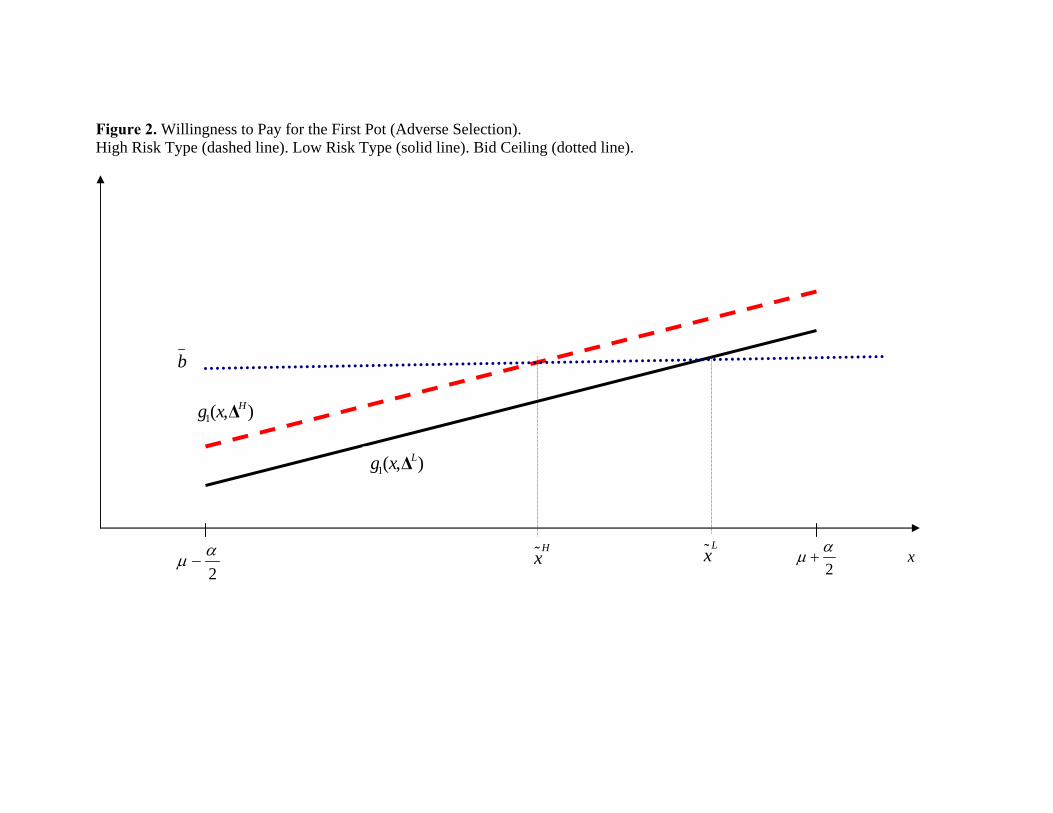
Figure 2. Willingness to Pay for the First Pot (Adverse Selection). High Risk Type (dashed line). Low Risk Type (solid line). Bid Ceiling (dotted line).

2αµ + x

1( , )Lg x ∆

2αµ −

1( , )Hg x ∆

b

LxH

x

Figure 3. Probability of Winning the First Auction with Adverse Selection

Panel A. Unrestricted Bidding.

Panel B. Restricted Bidding.

E CDH

I

45°

F G

BA 1( , )Hg x ∆1 ,

2Lg αµ ⎞⎛ −⎜ ⎟

⎝ ⎠∆

1 ,2

Lg αµ ⎞⎛ +⎜ ⎟⎝ ⎠

∆

1 ,2

Hg αµ ⎞⎛ +⎜ ⎟⎝ ⎠

∆1 ,2

Hg αµ ⎞⎛ −⎜ ⎟⎝ ⎠

∆ b

1( , )Lg x ∆

b

45°

F

E D C

BA 1( , )Hg x ∆1 ,

2Lg αµ ⎞⎛ −⎜ ⎟

⎝ ⎠∆

1 ,2

Lg αµ ⎞⎛ +⎜ ⎟⎝ ⎠

∆

1 ,2

Hg αµ ⎞⎛ +⎜ ⎟⎝ ⎠

∆1 ,2

Hg αµ ⎞⎛ −⎜ ⎟⎝ ⎠

∆

1( , )Lg x ∆

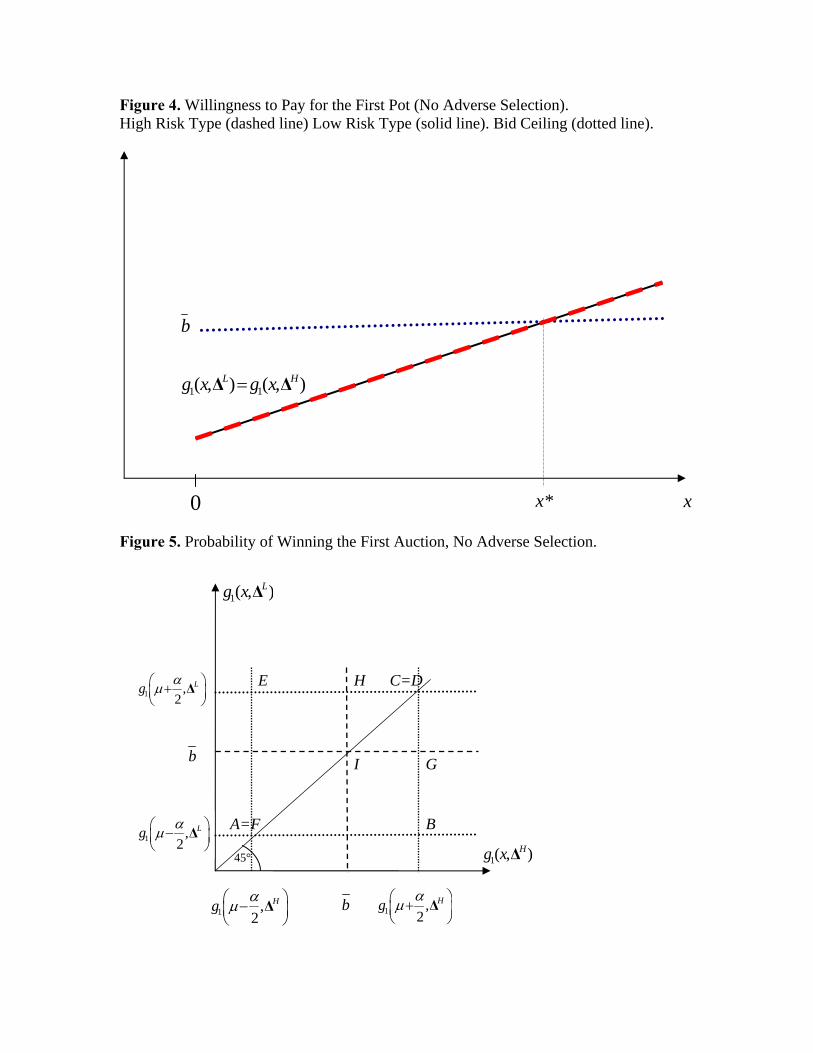
Figure 4. Willingness to Pay for the First Pot (No Adverse Selection). High Risk Type (dashed line) Low Risk Type (solid line). Bid Ceiling (dotted line).

Figure 5. Probability of Winning the First Auction, No Adverse Selection.

E C=D H

I

45°

G

BA=F

1( , )Hg x ∆1 ,

2Lg αµ ⎞⎛ −⎜ ⎟

⎝ ⎠∆

1 ,2

Lg αµ ⎞⎛ +⎜ ⎟⎝ ⎠

∆

1 ,2

Hg αµ ⎞⎛ +⎜ ⎟⎝ ⎠

∆1 ,2

Hg αµ ⎞⎛ −⎜ ⎟⎝ ⎠

∆ b

1( , )Lg x ∆

b

1 1( , ) ( , )L Hg x g x=∆ ∆

x0

b

*x

1 1[ ] [ ]cE Eθ θ=

Figure 6. Riskiness Profiles with Adverse Selection. Rosca with Unrestricted Bidding (dashed line) and Restricted Bidding (solid line).

Figure 7. Riskiness Profiles with No Adverse Selection.

2 2[ ] [ ]cE Eθ θ=

Round t 1 2

1 1[ ] [ ]cE Eθ θ=

2[ ]E θ

2[ ]cEθ

Round t

1[ ]cEθ

2

1[ ]E θ

1

Figure 8. Default Profiles, Rosca with Unrestricted Bidding (dashed line) and Restricted Bidding (solid line). Panel A. Adverse Selection, no Change in Rosca Composition.

Panel B. No Adverse Selection, Change in Rosca Composition.

1[ ]E Y

2[ ]E Y

2[ ]cE Y

Round t

1[ ]cE Y

21

2[ ]cE Y

2[ ]E Y

1[ ]E Y

Round t

1[ ]cE Y

2 1