Adversarial Search - Alan Ritteraritter.github.io/courses/5522_slides/advesarial_search.pdf ·...
134
Adversarial Search CS 5522: Artificial Intelligence II Instructor: Alan Ritter Ohio State University [These slides were adapted from CS188 Intro to AI at UC Berkeley. All materials available at http://ai.berkeley.edu.]
Transcript of Adversarial Search - Alan Ritteraritter.github.io/courses/5522_slides/advesarial_search.pdf ·...

Adversarial Search
CS 5522: Artificial Intelligence II
Instructor: Alan Ritter
Ohio State University [These slides were adapted from CS188 Intro to AI at UC Berkeley. All materials available at http://ai.berkeley.edu.]

Game Playing State-of-the-Art
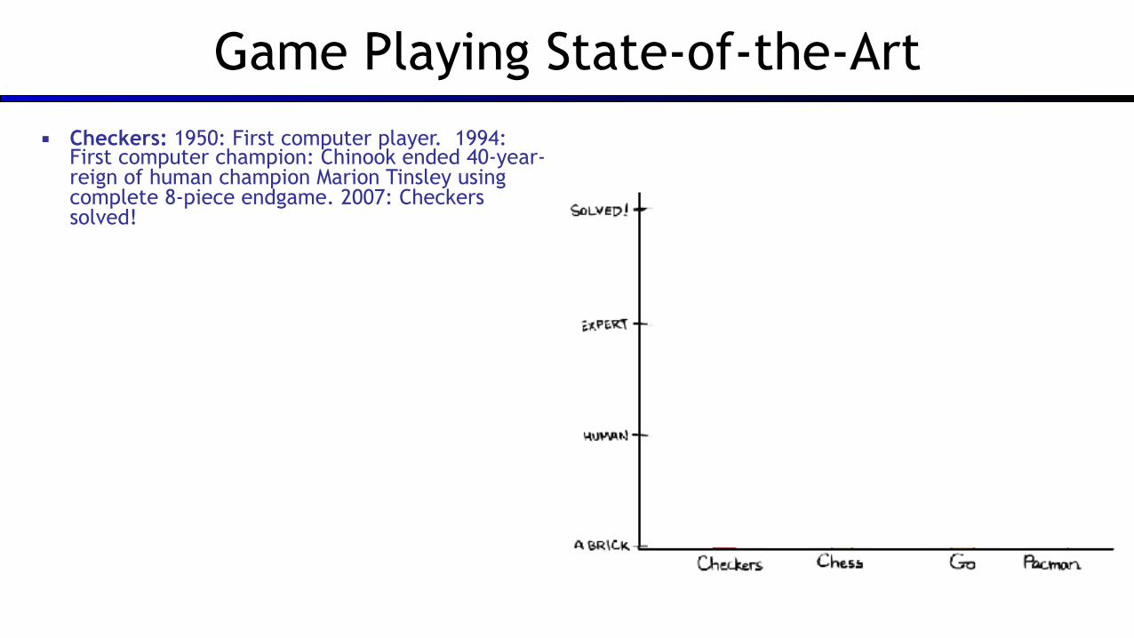
Game Playing State-of-the-Art▪ Checkers: 1950: First computer player. 1994:
First computer champion: Chinook ended 40-year-reign of human champion Marion Tinsley using complete 8-piece endgame. 2007: Checkers solved!

Game Playing State-of-the-Art▪ Checkers: 1950: First computer player. 1994:
First computer champion: Chinook ended 40-year-reign of human champion Marion Tinsley using complete 8-piece endgame. 2007: Checkers solved!

Game Playing State-of-the-Art▪ Checkers: 1950: First computer player. 1994:
First computer champion: Chinook ended 40-year-reign of human champion Marion Tinsley using complete 8-piece endgame. 2007: Checkers solved!
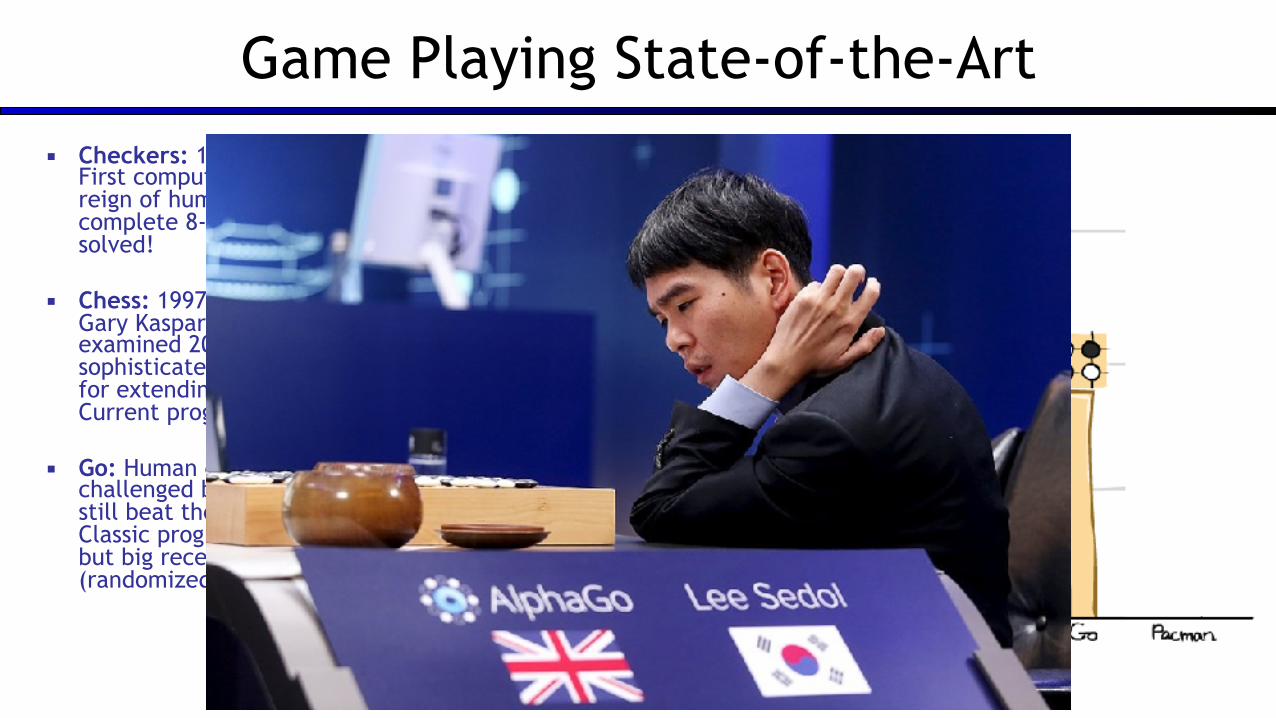
▪ Chess: 1997: Deep Blue defeats human champion Gary Kasparov in a six-game match. Deep Blue examined 200M positions per second, used very sophisticated evaluation and undisclosed methods for extending some lines of search up to 40 ply. Current programs are even better, if less historic.

Game Playing State-of-the-Art▪ Checkers: 1950: First computer player. 1994:
First computer champion: Chinook ended 40-year-reign of human champion Marion Tinsley using complete 8-piece endgame. 2007: Checkers solved!
▪ Chess: 1997: Deep Blue defeats human champion Gary Kasparov in a six-game match. Deep Blue examined 200M positions per second, used very sophisticated evaluation and undisclosed methods for extending some lines of search up to 40 ply. Current programs are even better, if less historic.
▪ Go: Human champions are now starting to be challenged by machines, though the best humans still beat the best machines. In go, b > 300! Classic programs use pattern knowledge bases, but big recent advances use Monte Carlo (randomized) expansion methods.
▪ Pacman

Behavior from Computation
[Demo: mystery pacman (L6D1)]
Adversarial Games

▪ Many different kinds of games!
▪ Axes: ▪ Deterministic or stochastic? ▪ One, two, or more players? ▪ Zero sum? ▪ Perfect information (can you see the state)?
▪ Want algorithms for calculating a strategy (policy) which recommends a move from each state
Types of Games

Deterministic Games
▪ Many possible formalizations, one is: ▪ States: S (start at s0) ▪ Players: P={1...N} (usually take turns) ▪ Actions: A (may depend on player / state) ▪ Transition Function: SxA → S ▪ Terminal Test: S → {t,f} ▪ Terminal Utilities: SxP → R
▪ Solution for a player is a policy: S → A

Zero-Sum Games
▪ Zero-Sum Games ▪ Agents have opposite utilities (values on outcomes) ▪ Lets us think of a single value that one maximizes
and the other minimizes ▪ Adversarial, pure competition
▪ General Games ▪ Agents have independent utilities (values on
outcomes) ▪ Cooperation, indifference, competition, and more
are all possible ▪ More later on non-zero-sum games

Adversarial Search

Single-Agent Trees

Single-Agent Trees

Single-Agent Trees

Single-Agent Trees

Single-Agent Trees
8

Single-Agent Trees
8
2 0 2 6 4 6… …

Value of a State
8
2 0 2 6 4 6… …

Value of a State
8
2 0 2 6 4 6… …
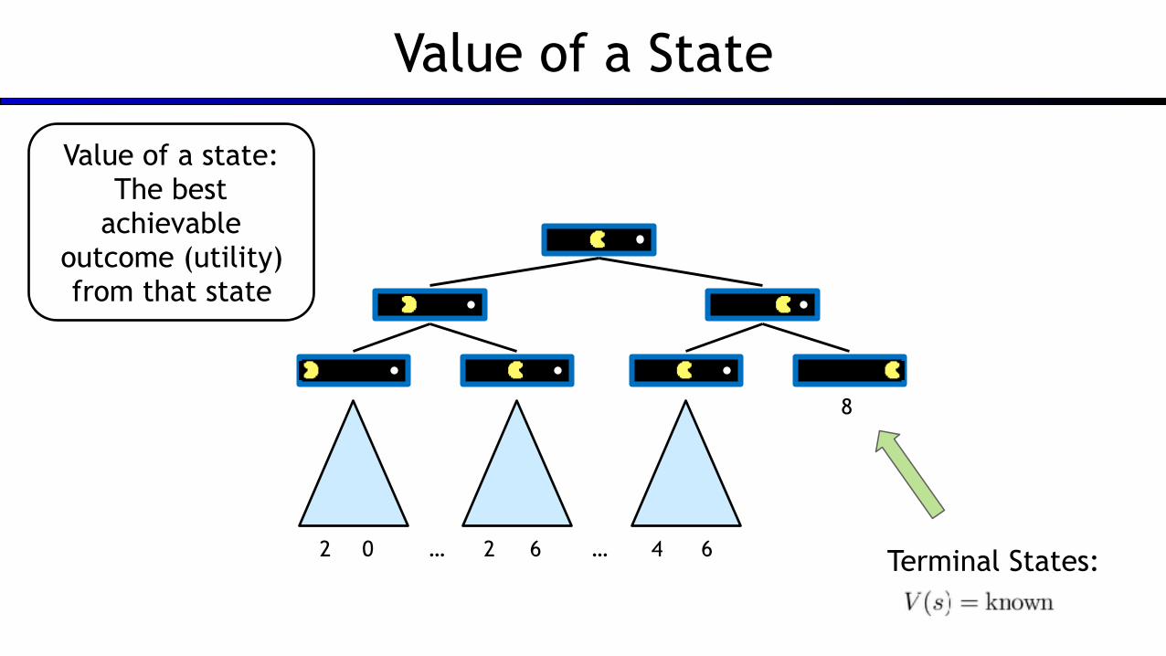
Value of a state: The best
achievable outcome (utility) from that state
Value of a State
8
2 0 2 6 4 6… … Terminal States:
Value of a state: The best
achievable outcome (utility) from that state

Value of a State
Non-Terminal States:
8
2 0 2 6 4 6… … Terminal States:
Value of a state: The best
achievable outcome (utility) from that state
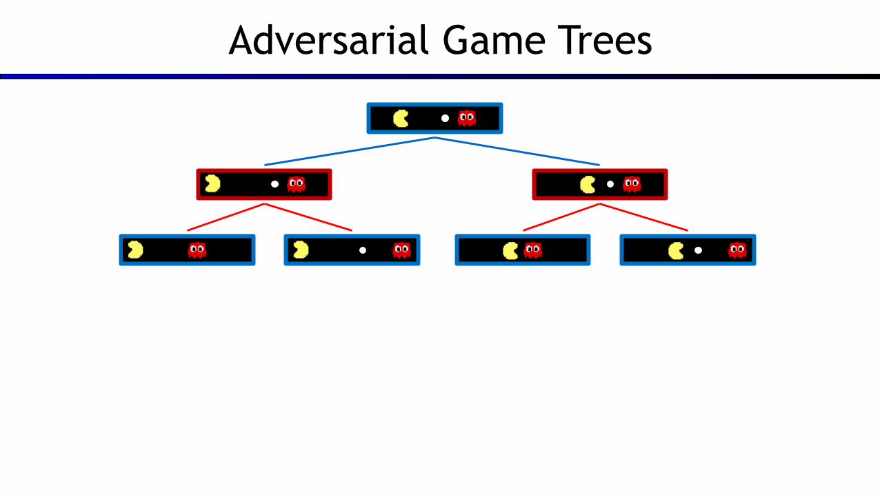
Adversarial Game Trees

Adversarial Game Trees

Adversarial Game Trees
Adversarial Game Trees

Adversarial Game Trees
-20 -8 -18 -5 -10 +4… … -20 +8

Minimax Values
+8-10-5-8

Minimax Values
+8-10-5-8
Terminal States:

Minimax Values
+8-10-5-8
Terminal States:
States Under Opponent’s Control:

Minimax Values
+8-10-5-8
States Under Agent’s Control:
Terminal States:
States Under Opponent’s Control:

Tic-Tac-Toe Game Tree

Adversarial Search (Minimax)
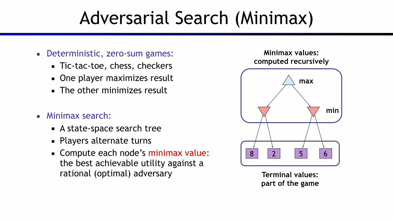
▪ Deterministic, zero-sum games: ▪ Tic-tac-toe, chess, checkers ▪ One player maximizes result ▪ The other minimizes result
▪ Minimax search: ▪ A state-space search tree ▪ Players alternate turns ▪ Compute each node’s minimax value:
the best achievable utility against a rational (optimal) adversary
8 2 5 6
max
min

Adversarial Search (Minimax)
▪ Deterministic, zero-sum games: ▪ Tic-tac-toe, chess, checkers ▪ One player maximizes result ▪ The other minimizes result
▪ Minimax search: ▪ A state-space search tree ▪ Players alternate turns ▪ Compute each node’s minimax value:
the best achievable utility against a rational (optimal) adversary
8 2 5 6
max
min
Terminal values: part of the game
Minimax values:computed recursively

Adversarial Search (Minimax)
▪ Deterministic, zero-sum games: ▪ Tic-tac-toe, chess, checkers ▪ One player maximizes result ▪ The other minimizes result
▪ Minimax search: ▪ A state-space search tree ▪ Players alternate turns ▪ Compute each node’s minimax value:
the best achievable utility against a rational (optimal) adversary
8 2 5 6
max
min2 5
5
Terminal values: part of the game
Minimax values:computed recursively

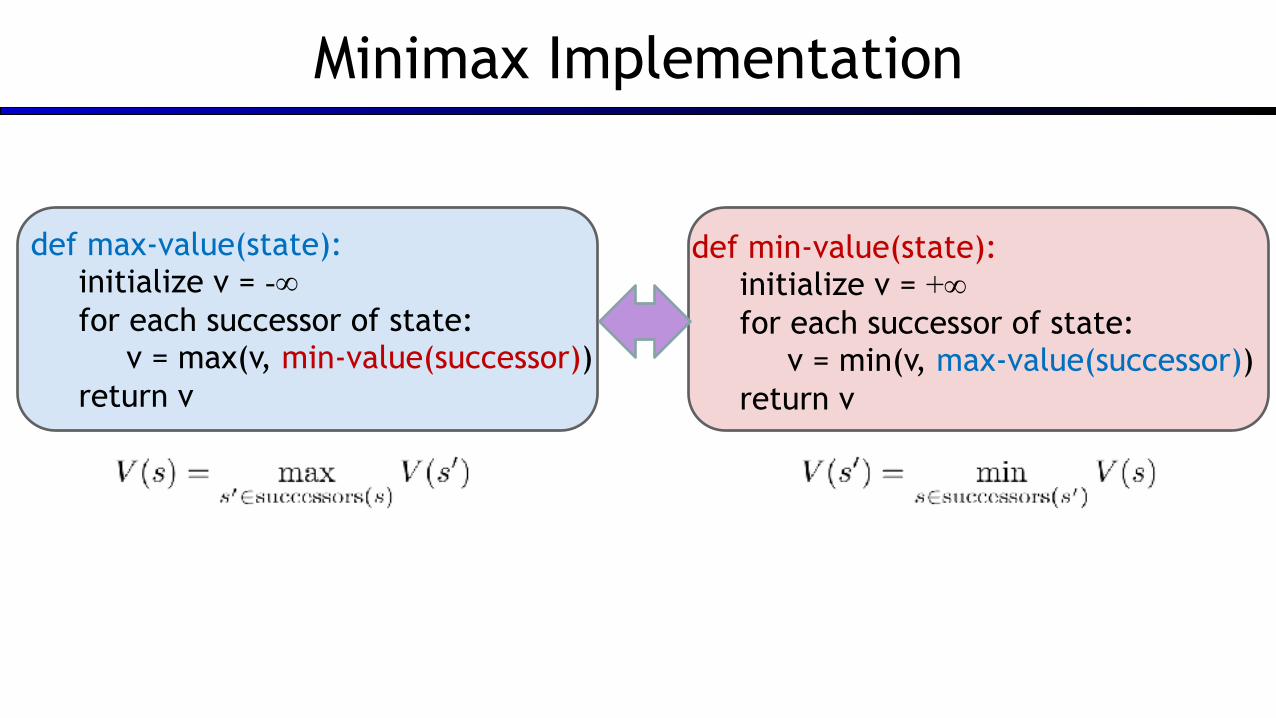
Minimax Implementation
def max-value(state): initialize v = -∞ for each successor of state:
v = max(v, min-value(successor)) return v

Minimax Implementation
def min-value(state): initialize v = +∞ for each successor of state:
v = min(v, max-value(successor)) return v
def max-value(state): initialize v = -∞ for each successor of state:
v = max(v, min-value(successor)) return v

Minimax Implementation
def min-value(state): initialize v = +∞ for each successor of state:
v = min(v, max-value(successor)) return v
def max-value(state): initialize v = -∞ for each successor of state:
v = max(v, min-value(successor)) return v
Minimax Implementation
def min-value(state): initialize v = +∞ for each successor of state:
v = min(v, max-value(successor)) return v
def max-value(state): initialize v = -∞ for each successor of state:
v = max(v, min-value(successor)) return v

Minimax Implementation (Dispatch)
def value(state): if the state is a terminal state: return the state’s utility if the next agent is MAX: return max-value(state) if the next agent is MIN: return min-value(state)

Minimax Implementation (Dispatch)
def value(state): if the state is a terminal state: return the state’s utility if the next agent is MAX: return max-value(state) if the next agent is MIN: return min-value(state)
def min-value(state): initialize v = +∞ for each successor of state:
v = min(v, value(successor)) return v
def max-value(state): initialize v = -∞ for each successor of state:
v = max(v, value(successor)) return v

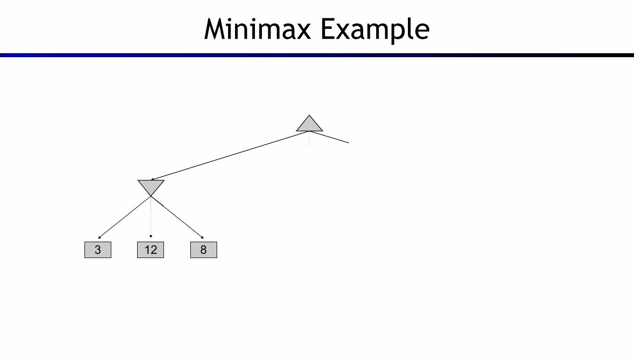
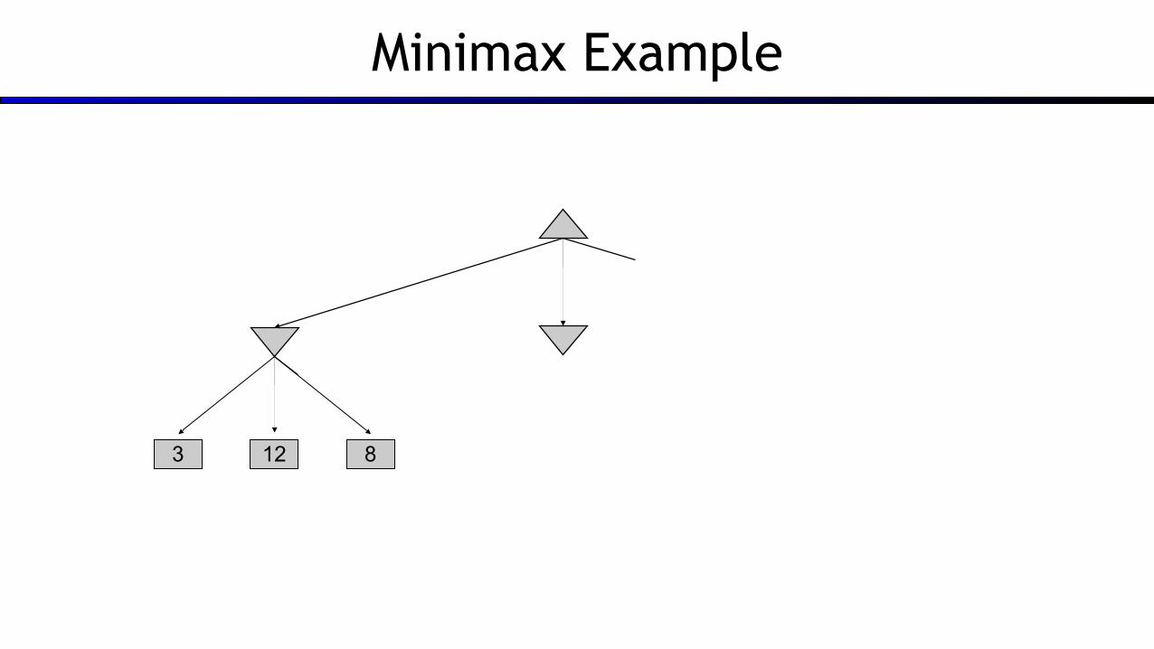
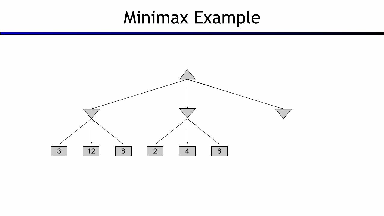
Minimax Example

Minimax Example

Minimax Example
3

Minimax Example
123
Minimax Example
12 83

Minimax Example
12 83
Minimax Example
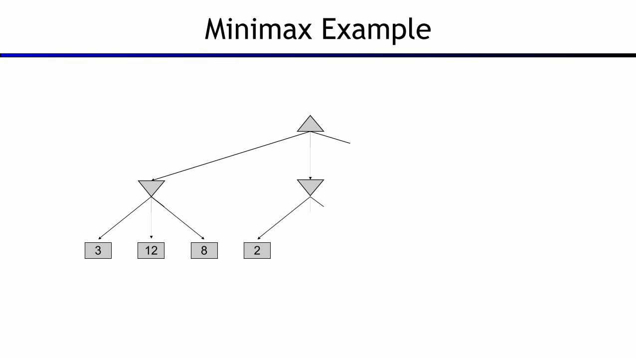
12 83 2

Minimax Example
12 83 2 4
Minimax Example
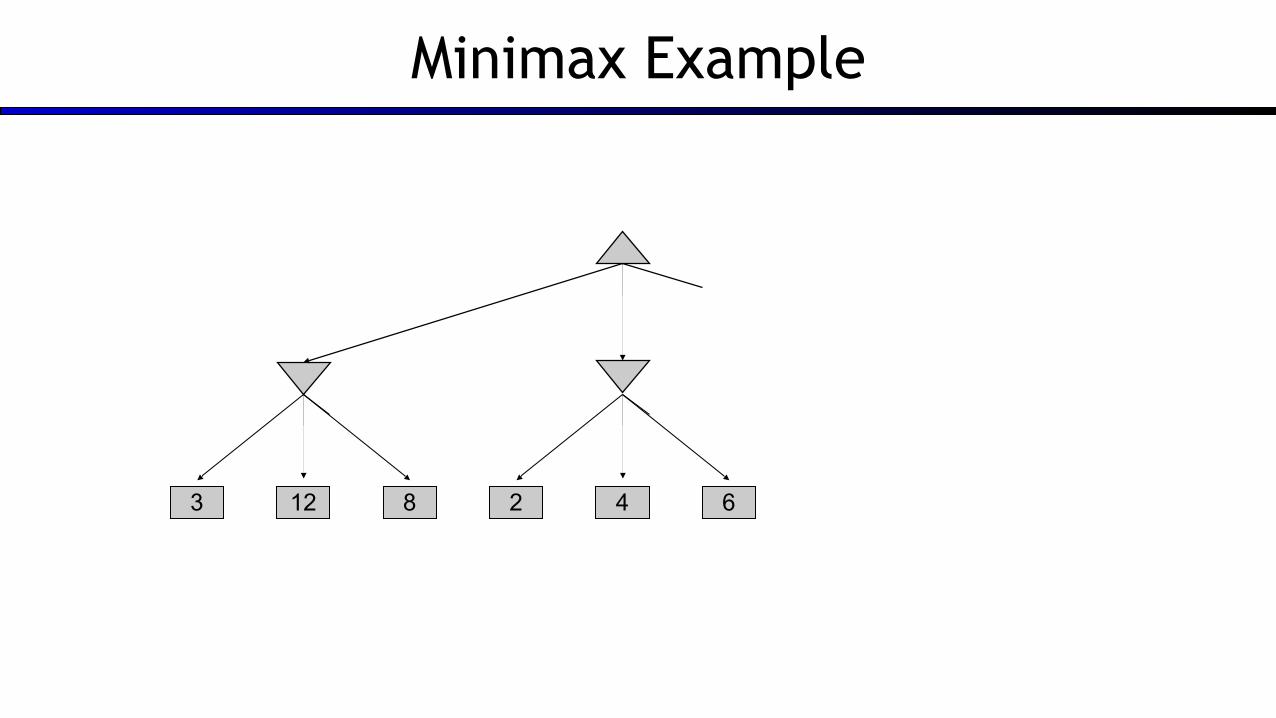
12 83 2 4 6

Minimax Example
12 83 2 4 6

Minimax Example
12 83 2 144 6

Minimax Example
12 8 53 2 144 6

Minimax Example
12 8 5 23 2 144 6
Minimax Efficiency
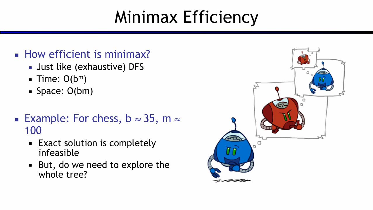
▪ How efficient is minimax? ▪ Just like (exhaustive) DFS ▪ Time: O(bm) ▪ Space: O(bm)
▪ Example: For chess, b ≈ 35, m ≈ 100 ▪ Exact solution is completely
infeasible ▪ But, do we need to explore the
whole tree?

Minimax Properties
Optimal against a perfect player. Otherwise?
10 10 9 100
max
min
[Demo: min vs exp (L6D2, L6D3)]

Minimax Properties
Optimal against a perfect player. Otherwise?
10 10 9 100
max
min
[Demo: min vs exp (L6D2, L6D3)]

Minimax Properties
Optimal against a perfect player. Otherwise?
10 10 9 100
max
min
[Demo: min vs exp (L6D2, L6D3)]

Video of Demo Min vs. Exp (Min)

Video of Demo Min vs. Exp (Min)

Video of Demo Min vs. Exp (Min)

Video of Demo Min vs. Exp (Exp)

Video of Demo Min vs. Exp (Exp)

Video of Demo Min vs. Exp (Exp)

Resource Limits

Resource Limits
▪ Problem: In realistic games, cannot search to leaves!
? ? ? ?
min
max

Resource Limits
▪ Problem: In realistic games, cannot search to leaves!
▪ Solution: Depth-limited search▪ Instead, search only to a limited depth in the tree▪ Replace terminal utilities with an evaluation function for non-
terminal positions
? ? ? ?
min
max

Resource Limits
▪ Problem: In realistic games, cannot search to leaves!
▪ Solution: Depth-limited search▪ Instead, search only to a limited depth in the tree▪ Replace terminal utilities with an evaluation function for non-
terminal positions
? ? ? ?
-1 -2 4 9
min
max

Resource Limits
▪ Problem: In realistic games, cannot search to leaves!
▪ Solution: Depth-limited search▪ Instead, search only to a limited depth in the tree▪ Replace terminal utilities with an evaluation function for non-
terminal positions
? ? ? ?
-1 -2 4 9
4
min
max
-2 4

Resource Limits
▪ Problem: In realistic games, cannot search to leaves!
▪ Solution: Depth-limited search▪ Instead, search only to a limited depth in the tree▪ Replace terminal utilities with an evaluation function for non-
terminal positions
▪ Example:▪ Suppose we have 100 seconds, can explore 10K nodes / sec▪ So can check 1M nodes per move▪ α-β reaches about depth 8 – decent chess program
▪ Guarantee of optimal play is gone
▪ More plies makes a BIG difference
▪ Use iterative deepening for an anytime algorithm? ? ? ?
-1 -2 4 9
4
min
max
-2 4

Depth Matters
▪ Evaluation functions are always imperfect
▪ The deeper in the tree the evaluation function is buried, the less the quality of the evaluation function matters
▪ An important example of the tradeoff between complexity of features and complexity of computation
[Demo: depth limited (L6D4, L6D5)]

Video of Demo Limited Depth (2)

Video of Demo Limited Depth (2)
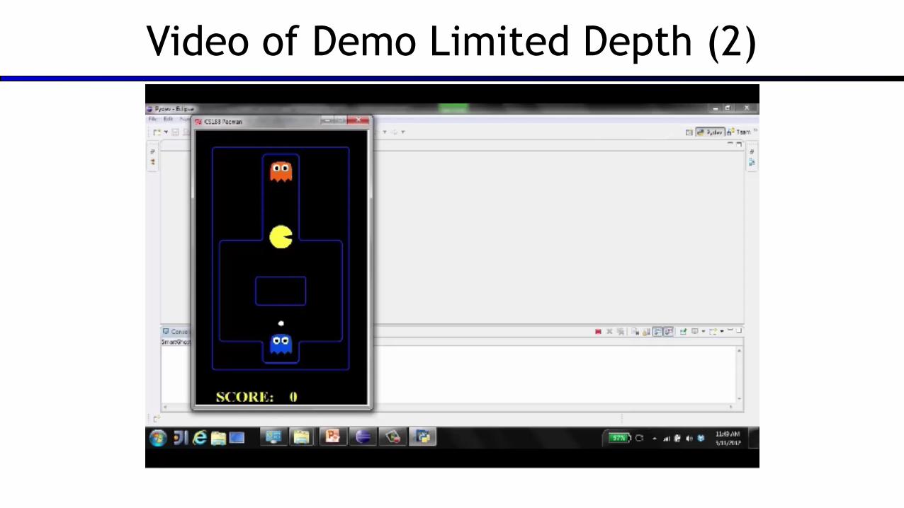
Video of Demo Limited Depth (2)

Video of Demo Limited Depth (10)

Video of Demo Limited Depth (10)

Video of Demo Limited Depth (10)

Evaluation Functions

Evaluation Functions
▪ Evaluation functions score non-terminals in depth-limited search
▪ Ideal function: returns the actual minimax value of the position ▪ In practice: typically weighted linear sum of features:
▪ e.g. f1(s) = (num white queens – num black queens), etc.

Evaluation for Pacman
[Demo: thrashing d=2, thrashing d=2 (fixed evaluation function), smart ghosts coordinate (L6D6,7,8,10)]

Evaluation for Pacman
[Demo: thrashing d=2, thrashing d=2 (fixed evaluation function), smart ghosts coordinate (L6D6,7,8,10)]

Evaluation for Pacman
[Demo: thrashing d=2, thrashing d=2 (fixed evaluation function), smart ghosts coordinate (L6D6,7,8,10)]

Evaluation for Pacman
[Demo: thrashing d=2, thrashing d=2 (fixed evaluation function), smart ghosts coordinate (L6D6,7,8,10)]

Evaluation for Pacman
[Demo: thrashing d=2, thrashing d=2 (fixed evaluation function), smart ghosts coordinate (L6D6,7,8,10)]

Video of Demo Thrashing (d=2)

Video of Demo Thrashing (d=2)

Video of Demo Thrashing (d=2)

Why Pacman Starves
▪ A danger of replanning agents! ▪ He knows his score will go up by eating the dot now (west, east) ▪ He knows his score will go up just as much by eating the dot later (east, west) ▪ There are no point-scoring opportunities after eating the dot (within the horizon, two here) ▪ Therefore, waiting seems just as good as eating: he may go east, then back west in the next
round of replanning!

Video of Demo Smart Ghosts (Coordination)

Video of Demo Smart Ghosts (Coordination)

Video of Demo Smart Ghosts (Coordination)

Video of Demo Smart Ghosts (Coordination) – Zoomed In

Video of Demo Smart Ghosts (Coordination) – Zoomed In
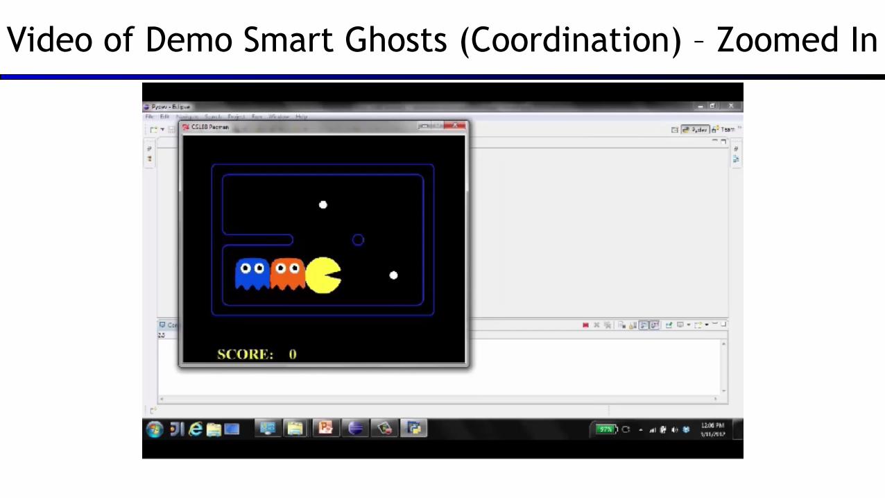
Video of Demo Smart Ghosts (Coordination) – Zoomed In
Game Tree Pruning

Minimax Example

Minimax Example

Minimax Example
3

Minimax Example
123

Minimax Example
12 83
Minimax Example
12 83

Minimax Example
12 83 2

Minimax Example
12 83 2 4

Minimax Example
12 83 2 4 6
Minimax Example
12 83 2 4 6

Minimax Example
12 83 2 144 6

Minimax Example
12 8 53 2 144 6

Minimax Example
12 8 5 23 2 144 6

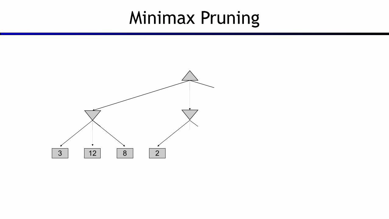
Minimax Pruning

Minimax Pruning

Minimax Pruning
3

Minimax Pruning
123

Minimax Pruning
12 83

Minimax Pruning
12 83
Minimax Pruning
12 83 2

Minimax Pruning
12 83 2

Minimax Pruning
12 83 2 14

Minimax Pruning
12 8 53 2 14

Minimax Pruning
12 8 5 23 2 14

Alpha-Beta Pruning
▪ General configuration (MIN version) ▪ We’re computing the MIN-VALUE at some node n ▪ We’re looping over n’s children ▪ n’s estimate of the childrens’ min is dropping ▪ Who cares about n’s value? MAX ▪ Let a be the best value that MAX can get at any
choice point along the current path from the root ▪ If n becomes worse than a, MAX will avoid it, so we
can stop considering n’s other children (it’s already bad enough that it won’t be played)
▪ MAX version is symmetric
MAX
MIN
MAX
MIN
a
n

Alpha-Beta Implementation
def min-value(state , α, β): initialize v = +∞ for each successor of state:
v = min(v, value(successor, α, β)) if v ≤ α return v β = min(β, v)
return v
def max-value(state, α, β): initialize v = -∞ for each successor of state:
v = max(v, value(successor, α, β)) if v ≥ β return v α = max(α, v)
return v
α: MAX’s best option on path to root β: MIN’s best option on path to root

Alpha-Beta Pruning Properties
▪ This pruning has no effect on minimax value computed for the root!
▪ Values of intermediate nodes might be wrong▪ Important: children of the root may have the wrong value▪ So the most naïve version won’t let you do action selection
10 10 0
max
min

Alpha-Beta Pruning Properties
▪ This pruning has no effect on minimax value computed for the root!
▪ Values of intermediate nodes might be wrong▪ Important: children of the root may have the wrong value▪ So the most naïve version won’t let you do action selection
▪ Good child ordering improves effectiveness of pruning
▪ With “perfect ordering”:▪ Time complexity drops to O(bm/2)▪ Doubles solvable depth!▪ Full search of, e.g. chess, is still hopeless…
▪ This is a simple example of metareasoning (computing about what to compute)
10 10 0
max
min


![EmotiGAN: Emoji Art using Generative Adversarial Networkscs229.stanford.edu/proj2017/final-reports/5244346.pdfA. Generative Adversarial Networks A Generative Adversarial Network[4]](https://static.fdocuments.us/doc/165x107/5ecde2ffc9dc5a794236dce0/emotigan-emoji-art-using-generative-adversarial-a-generative-adversarial-networks.jpg)