Pipe Flow/Friction Factor Calculations

using Excel Spreadsheets

Harlan H. Bengtson, PE, PhD

Emeritus Professor of Civil Engineering

Southern Illinois University Edwardsville

Table of Contents

Introduction

Section 1 – The Basic Equations

Section 2 – Laminar and Turbulent Flow in Pipes

Section 3 – Fully Developed Flow and the Entrance Region

Section 4 – Obtaining Friction Factor Values

Section 5 – Calculation of Frictional Head Loss and/or Frictional Pressure Drop

Section 6 – A Spreadsheet for Calculation of Pipe Flow Rate

Section 7 – A Spreadsheet for Calculation of Required Pipe Diameter

Summary

References

Introduction

The Darcy-Weisbach equation or the Fanning equation and the friction factor (Moody

friction factor or Fanning friction factor) are used for a variety of pressure pipe flow

calculations. Many of these types of calculations require a graphical and/or iterative

solution. The necessary iterative calculations can be carried out conveniently through the

use of a spreadsheet. This book starts with discussion of the Darcy-Weisbach and the

Fanning equations along with the parameters contained in them and the U.S. and S.I.

units typically used in the equations. Several example calculations are included and

spreadsheet screenshots are presented and discussed to illustrate the ways that

spreadsheets can be used for pressure pipe flow/friction factor calculations.

1. The Basic Equations

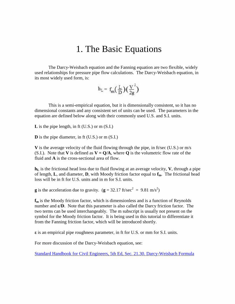
The Darcy-Weisbach equation and the Fanning equation are two flexible, widely

used relationships for pressure pipe flow calculations. The Darcy-Weisbach equation, in

its most widely used form, is:

This is a semi-empirical equation, but it is dimensionally consistent, so it has no

dimensional constants and any consistent set of units can be used. The parameters in the

equation are defined below along with their commonly used U.S. and S.I. units.

L is the pipe length, in ft (U.S.) or m (S.I.)

D is the pipe diameter, in ft (U.S.) or m (S.I.)

V is the average velocity of the fluid flowing through the pipe, in ft/sec (U.S.) or m/s

(S.I.). Note that V is defined as V = Q/A, where Q is the volumetric flow rate of the

fluid and A is the cross-sectional area of flow.

hL is the frictional head loss due to fluid flowing at an average velocity, V, through a pipe

of length, L, and diameter, D, with Moody friction factor equal to fm. The frictional head

loss will be in ft for U.S. units and in m for S.I. units.

g is the acceleration due to gravity. (g = 32.17 ft/sec2 = 9.81 m/s

2)

fm is the Moody friction factor, which is dimensionless and is a function of Reynolds

number and ε/D. Note that this parameter is also called the Darcy friction factor. The

two terms can be used interchangeably. The m subscript is usually not present on the

symbol for the Moody friction factor. It is being used in this tutorial to differentiate it

from the Fanning friction factor, which will be introduced shortly.

ε is an empirical pipe roughness parameter, in ft for U.S. or mm for S.I. units.

For more discussion of the Darcy-Weisbach equation, see:

Standard Handbook for Civil Engineers, 5th Ed, Sec. 21.30. Darcy-Weisbach Formula

A common form of the Fanning equation is:

Like the Darcy-Weisbach equation, the Fanning equation is also a semi-empirical,

dimensionally consistent equation. The parameters D, V, and L are the same as in the

Darcy-Weisbach equation just described above. The other parameters in the Fanning

equation are as follows:

is the density of the flowing fluid in lbm/ft3 for U.S. or kg/m

3 for S.I. units.

Pf is the frictional pressure drop due to the flowing fluid in lb/ft2 for U.S. or Pa for S.I.

units. (Note that lb is being used for a unit of force and lbm as a unit of mass in this

tutorial.)

ff is the Fanning friction factor, which is dimensionless and is a function of Reynolds

number and ε/D. The relationship between the Fanning friction factor and the Moody

friction factor is: fm = 4 ff. Note that the m and f subscripts are not typically used. The

symbol f is commonly used for both the Moody friction factor and the Fanning friction

factor. The subscripts are being used in this book to avoid confusion between the two

different friction factors, which are both in common use.

gc = 32.174 lbm-ft/lbf-sec2 [ a factor to convert force to (mass)x(acceleration ) ]

For more discussion of the Fanning equation, see: Perry's Chemical Engineers'

Handbook, 8th Ed. Sec 6.1.4. Incompressible Flow in Pipes and Channels

Values of ε for common pipe materials are available in many handbooks and

textbooks, as well as on a variety of websites. Table 1 below shows some typical values.

Table 1. Values of Pipe Roughness, ε

The surface roughness values in Table 1 came from the following two sources:

Perry's Chemical Engineers' Handbook, 8th Ed., Table 6-1 - S.I. units

Mark's Standard Handbook for Mechanical Engineers, 11th Ed., Table 3.3.9 - U.S. units

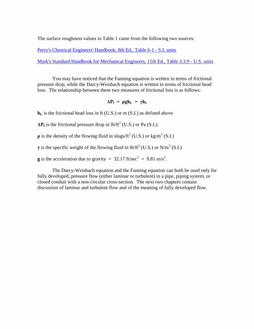
You may have noticed that the Fanning equation is written in terms of frictional

pressure drop, while the Darcy-Weisbach equation is written in terms of frictional head

loss. The relationship between these two measures of frictional loss is as follows:

ΔPf = ρghL = γhL

hL is the frictional head loss in ft (U.S.) or m (S.I.) as defined above

ΔPf is the frictional pressure drop in lb/ft2 (U.S.) or Pa (S.I.).

ρ is the density of the flowing fluid in slugs/ft3 (U.S.) or kg/m

3 (S.I.)

γ is the specific weight of the flowing fluid in lb/ft3 (U.S.) or N/m

3 (S.I.)

g is the acceleration due to gravity = 32.17 ft/sec2 = 9.81 m/s

2.

The Darcy-Weisbach equation and the Fanning equation can both be used only for

fully developed, pressure flow (either laminar or turbulent) in a pipe, piping system, or

closed conduit with a non-circular cross-section. The next two chapters contain

discussion of laminar and turbulent flow and of the meaning of fully developed flow.

2. Laminar and Turbulent Flow in Pipes

Determination of whether a given flow is laminar or turbulent is important for

several types of fluid flow situations. Here we will be concerned in particular with

pressure flow in pipes and whether a given flow is laminar or turbulent.

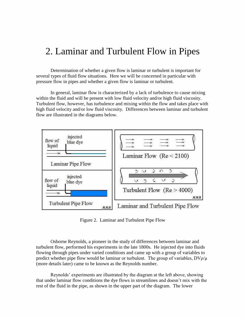
In general, laminar flow is characterized by a lack of turbulence to cause mixing

within the fluid and will be present with low fluid velocity and/or high fluid viscosity.

Turbulent flow, however, has turbulence and mixing within the flow and takes place with

high fluid velocity and/or low fluid viscosity. Differences between laminar and turbulent

flow are illustrated in the diagrams below.

Figure 2. Laminar and Turbulent Pipe Flow

Osborne Reynolds, a pioneer in the study of differences between laminar and

turbulent flow, performed his experiments in the late 1800s. He injected dye into fluids

flowing through pipes under varied conditions and came up with a group of variables to

predict whether pipe flow would be laminar or turbulent. The group of variables, DVρ/µ

(more details later) came to be known as the Reynolds number.

Reynolds’ experiments are illustrated by the diagram at the left above, showing

that under laminar flow conditions the dye flows in streamlines and doesn’t mix with the

rest of the fluid in the pipe, as shown in the upper part of the diagram. The lower

diagram illustrates turbulent flow, in which fluid turbulence mixes the dye throughout the

flowing fluid. The diagrams at the right are schematic illustrations of laminar flow with

straight streamlines and no turbulence and turbulent flow with eddy currents that mix the

flowing fluid.

The Reynolds number mentioned above is defined for pressure flow in pipes as

follows:

Re = DVρ/

The parameters in the equation and typical U.S. and S.I. units are:

D – the diameter of the pipe (ft – U.S. or m – S.I.)

V* – the average velocity of the fluid flowing in the pipe (ft/sec – U.S. or m/s – S.I.)

ρ – the density of the flowing fluid (slugs/ft3 – U.S. or kg/m

3 – S.I.)

µ – the dynamic viscosity of the flowing fluid (lb-sec/ft2 – U.S. or N-s/m

2 – S.I.)

*The average velocity is defined as V = Q/A, where Q is the volumetric flow rate

through the pipe and A is the cross-sectional area of flow.

The generally accepted criteria currently in use for laminar and turbulent flow in

pipes are as follow:

For Re < 2100 the flow will be laminar

For Re > 4000 the flow will be turbulent

For 2100 < Re < 4000 the flow may be either laminar or turbulent, depending upon

other factors such as the roughness of the pipe surface and the pipe entrance conditions.

This is called the transition region.

Pipe flow for transport of water, air or similar fluids is typically turbulent. Flow

of highly viscous fluids, such as lubricating oils, is often laminar. Since density and

viscosity are parameters in the Reynolds number, values for ρ and µ for the flowing fluid

are needed for pipe flow calculations. Values of density and viscosity for water from

32oF to 70

oF are given in the table below for use in example calculations in this tutorial.

To obtain density and viscosity values for a wide range of liquids see:

Table 2-32 in Perry's Chemical Engineers' Handbook, 8th Ed., for density values, and

Table 2-313 in Perry's Chemical Engineers' Handbook, 8th Ed., for viscosity values

Click below for a spreadsheet from which values of density and viscosity can be obtained

for any from a list of 73 liquids.

AccessEngineering Excel Spreadsheet for Incompressible Flow in Pipes and Channels

Table 2. Density and Viscosity of Water

Example #1: Determine whether the flow will be laminar or turbulent for flow of water

at 60oF at 0.8 cfs through a 6 inch diameter pipe.

Solution: For water at 60oF, the density and viscosity are: ρ = 1.938 slugs/ft

3 and

µ = 2.334 x 10-5

lb-sec/ft2.

The average velocity will be: V = Q/A = Q/(πD2/4) = 0.8/(π*(6/12)

2/4) = 4.07 ft/sec

The Reynolds number can now be calculated:

Re = DVρ/µ = ((6/12) ft)(4.07 ft/sec)(1.938 slugs/ft2)/(2.334 x 10

-5 lb-sec/ft

2)

Re = 1.69 x 106

Thus the flow is turbulent.

Note that the units all cancel out giving a dimensionless number when you use the fact

that 1 lb = 1 slug-ft/sec2.

3. Fully Developed Flow and the Entrance

Region

The entrance region for pipe flow is the portion of the pipe near the entry end, in

which the velocity profile is changing. This is illustrated in the diagram below for fluid

entering the pipe with a uniform velocity profile. Near the entrance, the fluid in the

center of the pipe remains uniform and is not affected by friction between the fluid and

the pipe wall. In the fully developed flow region (past the entrance region) the velocity

profile has reached its final shape and no longer changes.

Figure 3. The Entrance Length and Fully Developed Flow

As noted above, the Darcy Weisbach equation and the Fanning Equation apply

only to fully developed flow, which is the region past the entrance length. If the entrance

length is short in comparison with the total length of the pipe for which calculations are

being made, then the effect of the entrance region is commonly neglected and the total

pipe length is used for calculations. Additional head loss or pressure drop due to the

entrance region is typically calculated using an entrance loss coefficient. Discussion of

entrance loss coefficients, or minor loss coefficients in general is beyond the scope of this

tutorial.

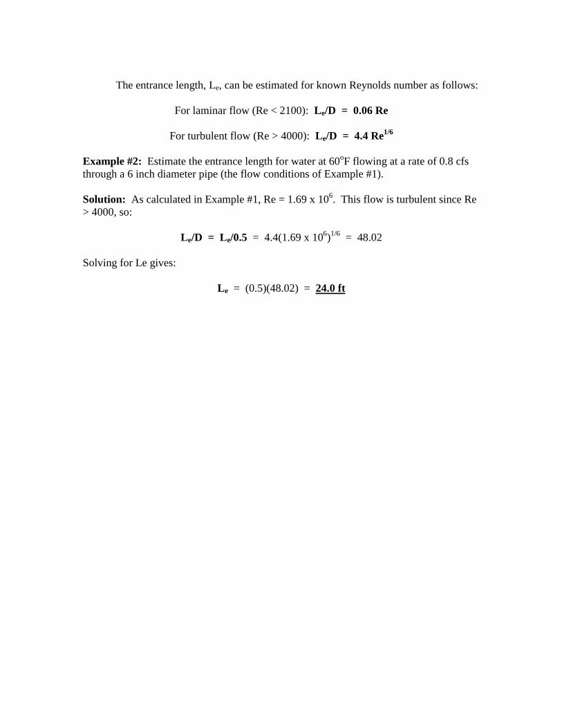
The entrance length, Le, can be estimated for known Reynolds number as follows:

For laminar flow (Re < 2100): Le/D = 0.06 Re

For turbulent flow (Re > 4000): Le/D = 4.4 Re1/6

Example #2: Estimate the entrance length for water at 60oF flowing at a rate of 0.8 cfs

through a 6 inch diameter pipe (the flow conditions of Example #1).

Solution: As calculated in Example #1, Re = 1.69 x 106. This flow is turbulent since Re

> 4000, so:

Le/D = Le/0.5 = 4.4(1.69 x 106)1/6

= 48.02

Solving for Le gives:

Le = (0.5)(48.02) = 24.0 ft

4. Obtaining Friction Factor Values

A value of the Moody friction factor is needed for most calculations with the

Darcy Weisbach equation and a value of the Fanning friction factor is needed for most

calculations with the Fanning equation. The exception is when the friction factor is being

determined empirically by measuring all of the other variables in the equation.

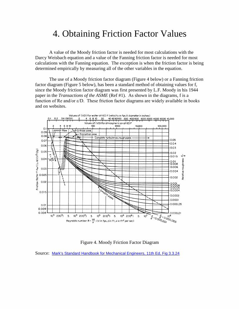
The use of a Moody friction factor diagram (Figure 4 below) or a Fanning friction

factor diagram (Figure 5 below), has been a standard method of obtaining values for f,

since the Moody friction factor diagram was first presented by L.F. Moody in his 1944

paper in the Transactions of the ASME (Ref #1). As shown in the diagrams, f is a

function of Re and/or ε/D. These friction factor diagrams are widely available in books

and on websites.

Figure 4. Moody Friction Factor Diagram

Source: Mark's Standard Handbook for Mechanical Engineers, 11th Ed, Fig 3.3.24

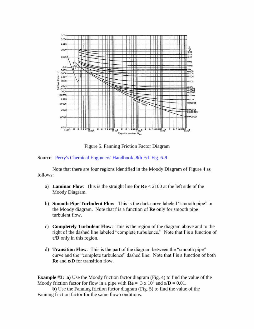
Figure 5. Fanning Friction Factor Diagram

Source: Perry's Chemical Engineers' Handbook, 8th Ed. Fig. 6-9

Note that there are four regions identified in the Moody Diagram of Figure 4 as

follows:

a) Laminar Flow: This is the straight line for Re < 2100 at the left side of the

Moody Diagram.

b) Smooth Pipe Turbulent Flow: This is the dark curve labeled “smooth pipe” in

the Moody diagram. Note that f is a function of Re only for smooth pipe

turbulent flow.

c) Completely Turbulent Flow: This is the region of the diagram above and to the

right of the dashed line labeled “complete turbulence.” Note that f is a function of

ε/D only in this region.

d) Transition Flow: This is the part of the diagram between the “smooth pipe”

curve and the “complete turbulence” dashed line. Note that f is a function of both

Re and ε/D for transition flow.

Example #3: a) Use the Moody friction factor diagram (Fig. 4) to find the value of the

Moody friction factor for flow in a pipe with Re = 3 x 106 and ε/D = 0.01.

b) Use the Fanning friction factor diagram (Fig. 5) to find the value of the

Fanning friction factor for the same flow conditions.

Solution: a) From the Moody Diagram in Figure 4, it can be seen that Re = 3 x 106 and

ε/D = 0.01 corresponds to fm = 0.038. Note that this is “completely turbulent flow.”

b) From the Fanning Diagram in Figure 5, it can be seen that Re = 3 x 106 and

ε/D = 0.01 corresponds to ff = 0.0095. Note that, as expected, fm = 4ff.

There is an alternative to graphical determination of the friction factor using a

Moody diagram or a Fanning diagram. There are equations for the friction factor in

terms of Re and/or ε/D. As shown on the diagrams, fm = 64/Re and ff = 16/Re for

laminar flow. The rest of this tutorial, however, will be devoted to the more complicated

case of turbulent flow.

The most general equation for friction factor under turbulent flow conditions is

the Colebook equation, shown below in its Moody friction factor form and in its Fanning

friction factor form. The turbulent flow portions of the Moody friction factor diagram

and the Fanning friction factor diagram are plots of the Colebrook equation.

fm = {(-2)log[(/3.7D) + (2.51/(Re*fm1/2

)]}-2

(Moody friction factor)

or: ff = {(-4)log[(/3.7D) + (1.256/(Re*ff1/2

)]}-2

(Fanning friction factor)

A difficult aspect of the Colebrook equation in either of the forms shown above is

that it cannot be solved explicitly for the friction factor (fm or ff), so an iterative solution

is required to calculate the friction factor for known values of Re and /D.

An approximation to the Colebrook equation is the Churchill equation, shown

below in its Moody and Fanning friction factor forms. These equations do not agree

quite as well with the friction factor diagrams over the entire turbulent flow range, but

have the advantage of being explicit for the friction factor (fm or ff).

fm = {(-2)log[(0.27/D) + (7/Re)0.9

]}-2

(Moody friction factor)

or: ff = {(-4)log[(0.27/D) + (7/Re)0.9

]}-2

(Fanning friction factor)

This presents the possibility of using the Churchill equation to obtain an initial

estimate of the friction factor and then use that estimate as the starting point for an

iterative solution with the Colebrook equation. This process works quite well and

converges rapidly to a solution as illustrated in the next two examples.

For further discussion of the Colebrook equation and the Churchill equation see:

Perry's Chemical Engineers' Handbook, 8th Ed. Equations (6-38) and (6-39) and

Mark's Standard Handbook for Mechanical Engineers, 11th Ed, Sec 3.3.11. Flow in Pipes

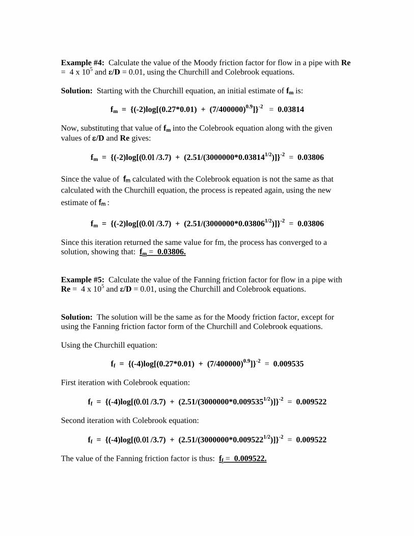
Example #4: Calculate the value of the Moody friction factor for flow in a pipe with Re

= 4 x 105 and ε/D = 0.01, using the Churchill and Colebrook equations.

Solution: Starting with the Churchill equation, an initial estimate of fm is:

fm = {(-2)log[(0.27*0.01) + (7/400000)0.9

]}-2

= 0.03814

Now, substituting that value of fm into the Colebrook equation along with the given

values of /D and Re gives:

fm = {(-2)log[(/3.7) + (2.51/(3000000*0.038141/2

)]}-2

= 0.03806

Since the value of fm calculated with the Colebrook equation is not the same as that

calculated with the Churchill equation, the process is repeated again, using the new

estimate of fm :

fm = {(-2)log[(/3.7) + (2.51/(3000000*0.038061/2

)]}-2

= 0.03806

Since this iteration returned the same value for fm, the process has converged to a

solution, showing that: fm = 0.03806.

Example #5: Calculate the value of the Fanning friction factor for flow in a pipe with

Re = 4 x 105 and ε/D = 0.01, using the Churchill and Colebrook equations.

Solution: The solution will be the same as for the Moody friction factor, except for

using the Fanning friction factor form of the Churchill and Colebrook equations.

Using the Churchill equation:

ff = {(-4)log[(0.27*0.01) + (7/400000)0.9

]}-2

= 0.009535

First iteration with Colebrook equation:

ff = {(-4)log[(/3.7) + (2.51/(3000000*0.0095351/2

)]}-2

= 0.009522

Second iteration with Colebrook equation:

ff = {(-4)log[(/3.7) + (2.51/(3000000*0.0095221/2

)]}-2

= 0.009522

The value of the Fanning friction factor is thus: ff = 0.009522.

An Excel workbook that automates the calculations shown in Example #4 and

Example #5 may be downloaded from the following link:

AccessEngineering Excel Spreadsheet for Incompressible Flow in Pipes and Channels

The use of this spreadsheet workbook for typical pipe flow calculations is

discussed and illustrated with examples in the next three sections.

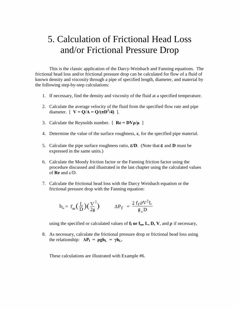
5. Calculation of Frictional Head Loss

and/or Frictional Pressure Drop

This is the classic application of the Darcy-Weisbach and Fanning equations. The

frictional head loss and/or frictional pressure drop can be calculated for flow of a fluid of

known density and viscosity through a pipe of specified length, diameter, and material by

the following step-by-step calculations:

1. If necessary, find the density and viscosity of the fluid at a specified temperature.

2. Calculate the average velocity of the fluid from the specified flow rate and pipe

diameter. [ V = Q/A = Q/(πD2/4) ].

3. Calculate the Reynolds number. [ Re = DVρ/µ ]

4. Determine the value of the surface roughness, ε, for the specified pipe material.

5. Calculate the pipe surface roughness ratio, ε/D. (Note that and D must be

expressed in the same units.)

6. Calculate the Moody friction factor or the Fanning friction factor using the

procedure discussed and illustrated in the last chapter using the calculated values

of Re and ε/D.

7. Calculate the frictional head loss with the Darcy Weisbach equation or the

frictional pressure drop with the Fanning equation:

using the specified or calculated values of ff or fm, L, D, V, and if necessary,

8. As necessary, calculate the frictional pressure drop or frictional head loss using

the relationship: ΔPf = ρghL = γhL.

These calculations are illustrated with Example #6.

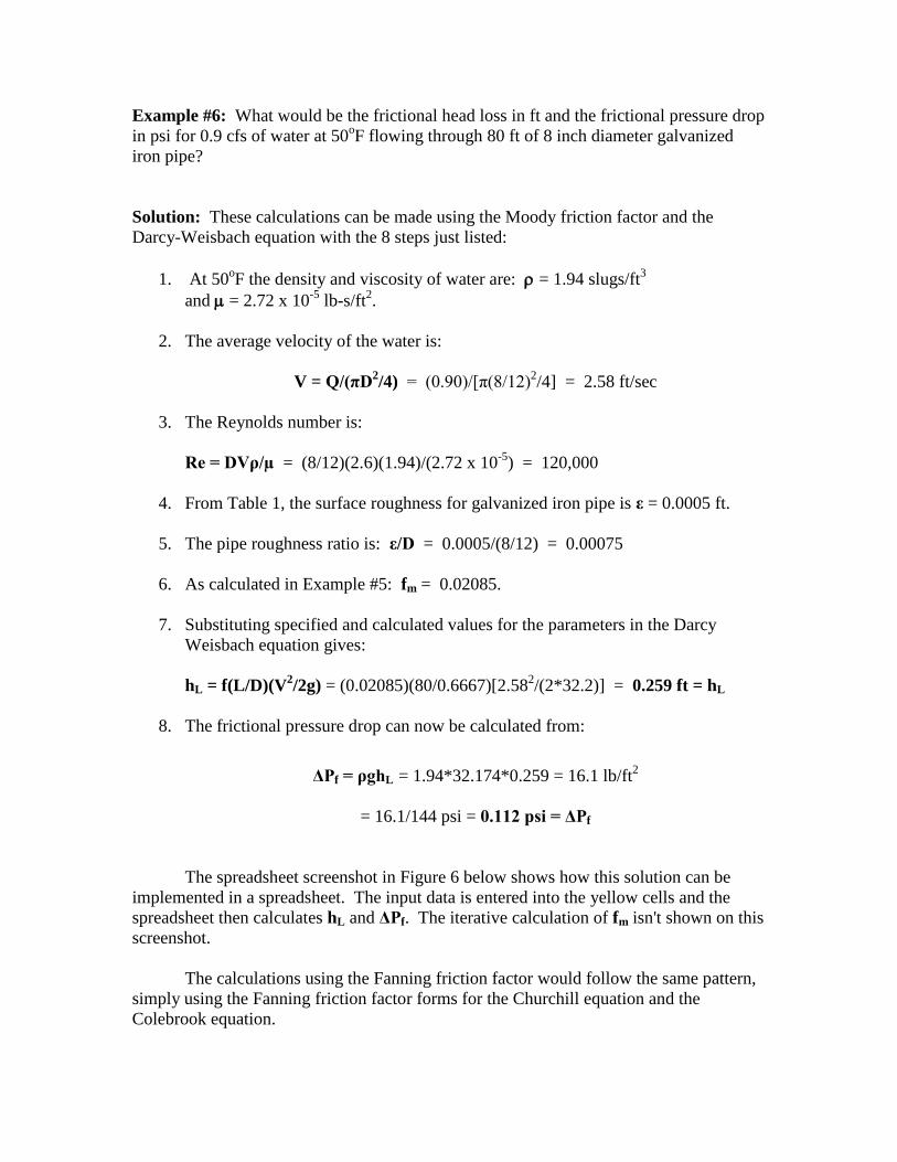
Example #6: What would be the frictional head loss in ft and the frictional pressure drop

in psi for 0.9 cfs of water at 50oF flowing through 80 ft of 8 inch diameter galvanized

iron pipe?

Solution: These calculations can be made using the Moody friction factor and the

Darcy-Weisbach equation with the 8 steps just listed:

1. At 50oF the density and viscosity of water are: = 1.94 slugs/ft

3

and = 2.72 x 10-5

lb-s/ft2.

2. The average velocity of the water is:

V = Q/(πD2/4) = (0.90)/[π(8/12)

2/4] = 2.58 ft/sec

3. The Reynolds number is:

Re = DVρ/µ = (8/12)(2.6)(1.94)/(2.72 x 10-5

) = 120,000

4. From Table 1, the surface roughness for galvanized iron pipe is ε = 0.0005 ft.

5. The pipe roughness ratio is: ε/D = 0.0005/(8/12) = 0.00075

6. As calculated in Example #5: fm = 0.02085.

7. Substituting specified and calculated values for the parameters in the Darcy

Weisbach equation gives:

hL = f(L/D)(V2/2g) = (0.02085)(80/0.6667)[2.58

2/(2*32.2)] = 0.259 ft = hL

8. The frictional pressure drop can now be calculated from:

ΔPf = ρghL = 1.94*32.174*0.259 = 16.1 lb/ft2

= 16.1/144 psi = 0.112 psi = ΔPf

The spreadsheet screenshot in Figure 6 below shows how this solution can be

implemented in a spreadsheet. The input data is entered into the yellow cells and the

spreadsheet then calculates hL and ΔPf. The iterative calculation of fm isn't shown on this

screenshot.

The calculations using the Fanning friction factor would follow the same pattern,

simply using the Fanning friction factor forms for the Churchill equation and the

Colebrook equation.

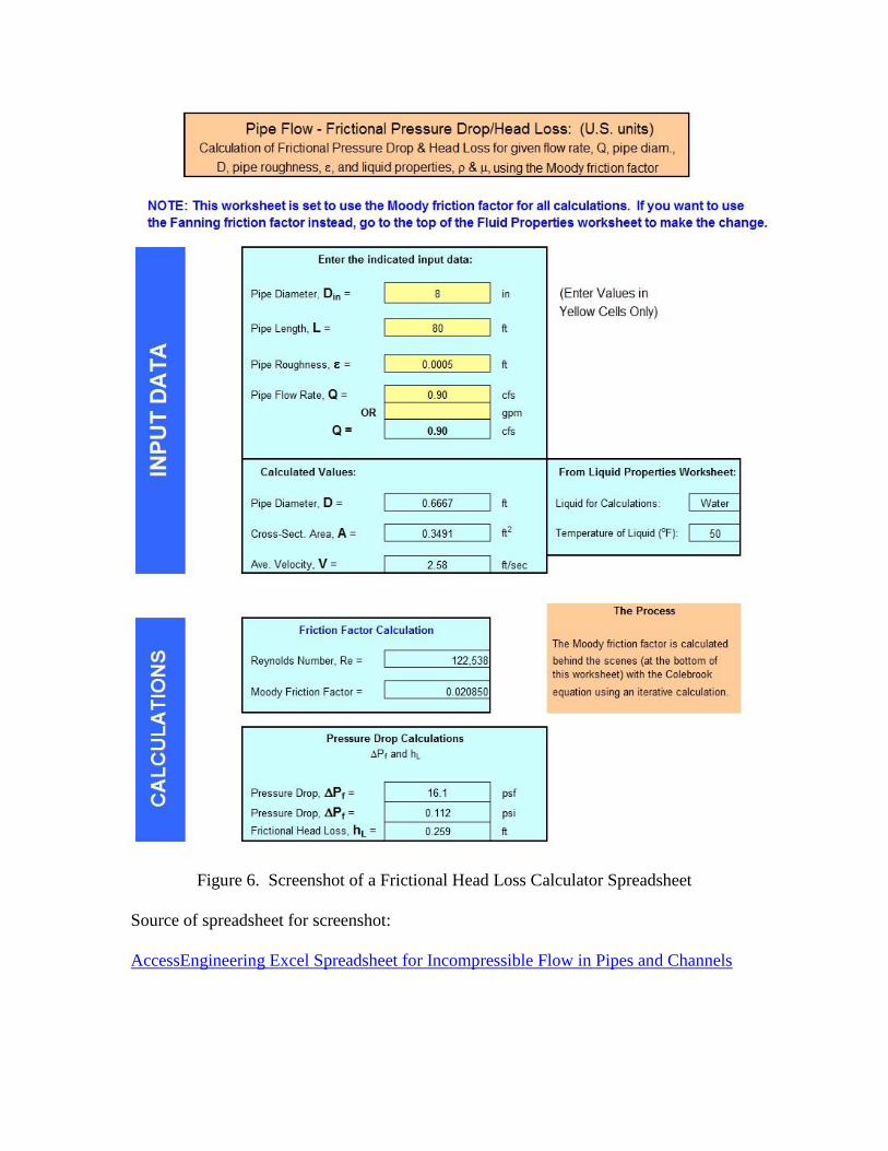
Figure 6. Screenshot of a Frictional Head Loss Calculator Spreadsheet

Source of spreadsheet for screenshot:

AccessEngineering Excel Spreadsheet for Incompressible Flow in Pipes and Channels

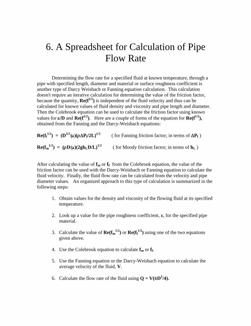
6. A Spreadsheet for Calculation of Pipe

Flow Rate

Determining the flow rate for a specified fluid at known temperature, through a

pipe with specified length, diameter and material or surface roughness coefficient is

another type of Darcy Weisbach or Fanning equation calculation. This calculation

doesn't require an iterative calculation for determining the value of the friction factor,

because the quantity, Re(f1/2

) is independent of the fluid velocity and thus can be

calculated for known values of fluid density and viscosity and pipe length and diameter.

Then the Colebrook equation can be used to calculate the friction factor using known

values for /D and Re(f1/2

). Here are a couple of forms of the equation for Re(f1/2

),

obtained from the Fanning and the Darcy-Weisbach equations:

Re(ff1/2

) = (D3/2

/)(Pf/2L)1/2

( for Fanning friction factor; in terms of Pf )

Re(fm1/2

) = (D/)(2ghLD/L)1/2

( for Moody friction factor; in terms of hL )

After calculating the value of fm or ff from the Colebrook equation, the value of the

friction factor can be used with the Darcy-Weisbach or Fanning equation to calculate the

fluid velocity. Finally, the fluid flow rate can be calculated from the velocity and pipe

diameter values. An organized approach to this type of calculation is summarized in the

following steps:

1. Obtain values for the density and viscosity of the flowing fluid at its specified

temperature.

2. Look up a value for the pipe roughness coefficient, ε, for the specified pipe

material.

3. Calculate the value of Re(fm1/2

) or Re(ff1/2

) using one of the two equations

given above.

4. Use the Colebrook equation to calculate fm or ff.

5. Use the Fanning equation or the Darcy-Weisbach equation to calculate the

average velocity of the fluid, V.

6. Calculate the flow rate of the fluid using Q = V(D2/4).

Example #9: Calculate the flow rate of 50oF water due to a head of 1.2 ft across 80 ft of

6 inch diameter galvanized iron pipe.

Solution: The spreadsheet screenshot in Figure 7 shows the solution to this example.

All of the 6 steps shown above are included in the spreadsheet solution.

1. For the Access Engineering pipe flow calculations spreadsheet, which is the source for

the screenshot in Figure 7, the first step is completed by selecting a fluid and entering the

fluid temperature on a Fluid Properties worksheet. The fluid density and viscosity are

then available for use in the other worksheets.

2. The surface roughness for the pipe may be obtained from Table 1 in Chapter1, or from

the sources shown for the values in Table 1. The value of , needs to be entered into the

indicated yellow cell, along with the pipe diameter, pipe length, and allowable head loss,

each in its respective yellow cell.

3. The value of Re(ff1/2

) calculated by the spreadsheet, using the equation shown near

the beginning of this chapter, and shown in the screenshot, is 12381

4. The value of the Fanning friction factor calculated by the spreadsheet, using the

Colebrook equation, and shown in the screenshot, is 0.00531.

5. The fluid velocity is calculated by the spreadsheet using the Fanning equation, and is

shown in the screenshot to be: 4.8 ft/sec

6. Finally, the fluid flow rate is calculated by the spreadsheet using Q = VA, and shown

in the screenshot to be 0.94 cfs. The spreadsheet also includes unit conversion to gpm,

with a value of 420 gpm.

Figure 7. Screenshot of a Flow Rate Calculator Spreadsheet

Source of spreadsheet for screenshot:

AccessEngineering Excel Spreadsheet for Incompressible Flow in Pipes and Channels

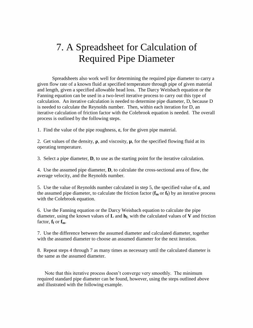
7. A Spreadsheet for Calculation of

Required Pipe Diameter

Spreadsheets also work well for determining the required pipe diameter to carry a

given flow rate of a known fluid at specified temperature through pipe of given material

and length, given a specified allowable head loss. The Darcy Weisbach equation or the

Fanning equation can be used in a two-level iterative process to carry out this type of

calculation. An iterative calculation is needed to determine pipe diameter, D, because D

is needed to calculate the Reynolds number. Then, within each iteration for D, an

iterative calculation of friction factor with the Colebrook equation is needed. The overall

process is outlined by the following steps.

1. Find the value of the pipe roughness, ε, for the given pipe material.

2. Get values of the density, ρ, and viscosity, µ, for the specified flowing fluid at its

operating temperature.

3. Select a pipe diameter, D, to use as the starting point for the iterative calculation.

4. Use the assumed pipe diameter, D, to calculate the cross-sectional area of flow, the

average velocity, and the Reynolds number.

5. Use the value of Reynolds number calculated in step 5, the specified value of , and

the assumed pipe diameter, to calculate the friction factor (fm or ff) by an iterative process

with the Colebrook equation.

6. Use the Fanning equation or the Darcy Weisbach equation to calculate the pipe

diameter, using the known values of L and hL with the calculated values of V and friction

factor, ff or fm.

7. Use the difference between the assumed diameter and calculated diameter, together

with the assumed diameter to choose an assumed diameter for the next iteration.

8. Repeat steps 4 through 7 as many times as necessary until the calculated diameter is

the same as the assumed diameter.

Note that this iterative process doesn’t converge very smoothly. The minimum

required standard pipe diameter can be found, however, using the steps outlined above

and illustrated with the following example.

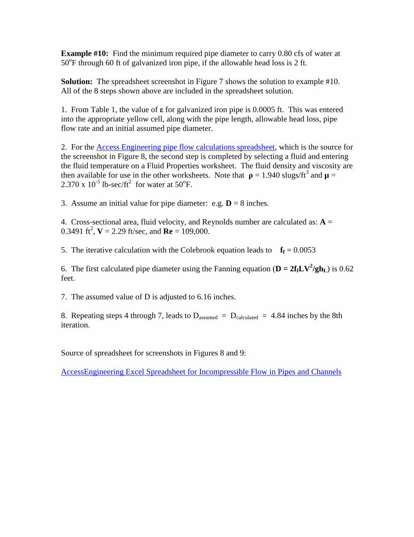
Example #10: Find the minimum required pipe diameter to carry 0.80 cfs of water at

50oF through 60 ft of galvanized iron pipe, if the allowable head loss is 2 ft.

Solution: The spreadsheet screenshot in Figure 7 shows the solution to example #10.

All of the 8 steps shown above are included in the spreadsheet solution.

1. From Table 1, the value of ε for galvanized iron pipe is 0.0005 ft. This was entered

into the appropriate yellow cell, along with the pipe length, allowable head loss, pipe

flow rate and an initial assumed pipe diameter.

2. For the Access Engineering pipe flow calculations spreadsheet, which is the source for

the screenshot in Figure 8, the second step is completed by selecting a fluid and entering

the fluid temperature on a Fluid Properties worksheet. The fluid density and viscosity are

then available for use in the other worksheets. Note that ρ = 1.940 slugs/ft3 and µ =

2.370 x 10-5

lb-sec/ft2 for water at 50

oF.

3. Assume an initial value for pipe diameter: e.g. D = 8 inches.

4. Cross-sectional area, fluid velocity, and Reynolds number are calculated as: A =

0.3491 ft2, V = 2.29 ft/sec, and Re = 109,000.

5. The iterative calculation with the Colebrook equation leads to ff = 0.0053

6. The first calculated pipe diameter using the Fanning equation (D = 2ffLV2/ghL) is 0.62

feet.

7. The assumed value of D is adjusted to 6.16 inches.

8. Repeating steps 4 through 7, leads to Dassumed = Dcalculated = 4.84 inches by the 8th

iteration.

Source of spreadsheet for screenshots in Figures 8 and 9:

AccessEngineering Excel Spreadsheet for Incompressible Flow in Pipes and Channels

Figure 8. Screenshot of a Pipe Diameter Calculator Spreadsheet – Part 1

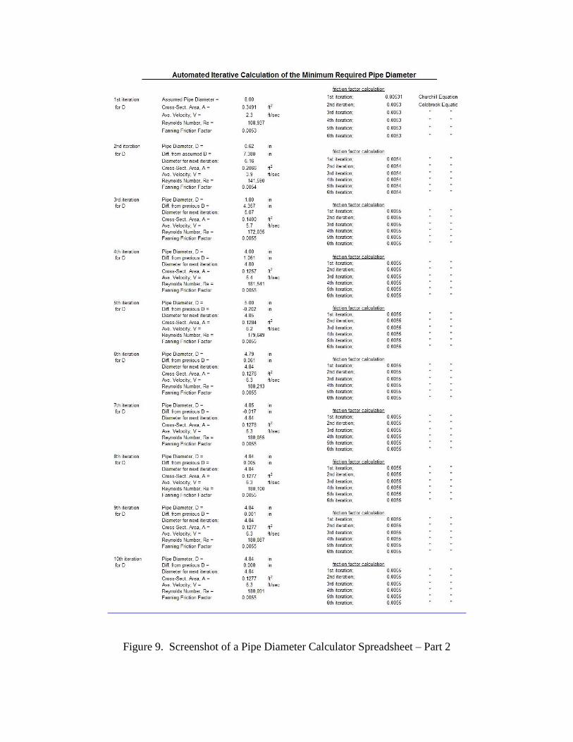
Figure 9. Screenshot of a Pipe Diameter Calculator Spreadsheet – Part 2

Summary

The Darcy-Weisbach equation or Fanning equation can be used together with the

Moody friction factor or the Fanning friction factor to make calculations involving the

pipe flow variables, pipe length, L; pipe diameter, D, pipe roughness, ε, fluid flow rate,

Q; frictional head loss, hL or frictional pressure drop, Pf, average fluid velocity, V; and

fluid properties (density and viscosity), as discussed in this tutorial. Spreadsheets are a

very convenient method for making these calculations because iterative solutions are

required for some of the equations. The three major types of calculations discussed and

illustrated with examples and spreadsheet screenshots in this tutorial are i) calculation of

frictional head loss or frictional pressure drop, ii) calculation of fluid flow rate, and iii)

calculation of minimum required pipe diameter. Each of these can be determined if the

other parameters are known.

References

1. Green, D.W. & Perry, R.H., Perry’s Chemical Engineers’ Handbook, 8th Ed., New

York: McGraw-Hill Book Company, 2008. Sec. 6.1.4. Incompressible Flow in Pipes and

Channels

2. Avallone, E.A., Baumeister III, T. & Sadegh, A., Marks’ Standard Handbook for

Mechanical Engineers, 11th

Ed., New York, McGraw-Hill Book Company, 2006.

Sec. 3.3.11. Flow in Pipes.

3. Ricketts, J.T., Loftin, M.K., & Merritt, F.S., Standard Handbook for Civil Engineers,

New York, McGraw-Hill Book Company, 2004.

Sec. 21.3 Pipe Flow

4. Hicks, T.G., Chopey, N.P., Handbook of Chemical Engineering Calculations, 4th Ed.,

New York, McGraw-Hill Book Company, 2012.

Sec. 6.4. Determining the Pressure Loss in Pipes.

5. Bengtson, Harlan H., Spreadsheet Use for Pipe Flow-Friction Factor Calculations, an

online, continuing education course for PDH credit.