Subject Mediation for Integrated Access to Heterogeneous Information Sources

1/29/2016
1
ADVANCES IN WITHIN-SUBJECT MEDIATION ANALYSIS
Andrew F. Hayes and Kristopher J. Preacher, co-chairs
Authors and Presenters
Andrew F. Hayes*, Ph.D., The Ohio State University
Amanda K. Montoya*, The Ohio State University
Kristopher J. Preacher*, Ph.D, Vanderbilt University
James P. Selig, Ph.D., University of Arkansas
Elizabeth Page-Gould, Ph.D., University of Toronto
Amanda Sharples*, University of Toronto
* presenter
• In this symposium, we each address statistical approaches to mediation analysis in studies that involve repeated measurement of X, M, or Y rather than merely observed or manipulated cross-sectionally and measured only once.
X YM
In the interest of time, please save your questions for the Q&A period.
• a path-analytic approach to quantifying and testing indirect effects in the two-condition experiment where M and Y are repeatedly measured in people assigned to both conditions of X (Hayes and Montoya).
• multilevel random-effects mediation models when X, M, and Y are repeatedly measured on the same person using a variety of stimuli or in a variety of situations (Page-Gould and Sharples).
• an empirical approach to examining the problem of determining the effect of measurement lag on indirect effects (Preacher and Selig).
Specifically, we address…
a b
c'

1/29/2016
2
STRATEGIES FOR INCORPORATING LAG AS MODERATOR IN MEDIATION MODELS
Kristopher J. PreacherVanderbilt University
James P. SeligUniversity of Arkansas for Medical Sciences
Consider the simple mediation model commonly used in social and personality psychology studies:
This model has great heuristic value. Yetmethodologists have had much to say about theinadequacy of this model for drawing causalconclusions.
Perhaps the biggest limitation is that many designsassess X, M, and Y simultaneously, or nearly so.
Yet, causes need time to exert their effects (Hume, 1738).Y
X
M
The common “simple mediation” model
a
b
c'

1/29/2016
3
We could stagger the assessments of X, M, and Y in time, allowing time for the effect and to be more confident when saying things like “Xcauses Y indirectly through M” or “M mediates the effect of X on Y.”
Y
X
M
time
With measurement staggered in time
a
b
c'
Controlling for prior measurements of Mand Y is also recommended. This helps separate out the stable variance in Mand Y, which cannot be explained by other predictors.
Y3
X1
M2
time
M1
Y1
Adding covariance adjustment for prior measurements
a
b
c'

1/29/2016
4
Combining these recommendations leads to the popular cross-lagged panel model (CLPM) approach to assessing mediation (Cole & Maxwell, 2003).
Y3
time
Y1
M3
X3X1
M2M1
Y2
X2
The cross-lagged panel mediation model
The CLPM is a more defensible method for assessing mediation. However, it still suffers from a major problem—the effects in such models depend on the chosen lag, or how much time elapses between the assessments of X, M, and Y.
From Voelkle et al. (2012):
Two researchers studyingthe same variables use twodifferent lags (1 vs. 2 mos.)and draw different conclu-sions about the strengthof the X→Y and Y→X effects.
Effects are not invariant to choice of time lag

1/29/2016
5
In the context of regression (X→Y), Selig, Preacher, & Little (2012) proposed using a variable-lag design, such that the assessment of either X or Y (or both) are deliberately staggered over time allowing lags to vary across persons.
The result is a lag as moderator (LAM) analysis, in which we explicitly model how the X→Y effect changes as a function of lag. Lag itself is treated as a moderator.
This can yield greater insight into the causal process, and can explain why different researchers arrive at different conclusions as a function of the arbitrary amount of time that elapses between the assessment of different variables.
YX
Lag
Lag as moderator (LAM) analysis
Here is how it works. Rather than using:
We proposed instead using:
...an example of a standard interaction model, where is the simple slope relating X to Y at a given lag.
This model requires individual differences in lag, which can be either observational or experimentally manipulated.
0 1ˆi iY b b X
0 1 2 3
0 2 1 3
ˆi i i i i
i i i
Y b b X b Lag b X Lag
b b Lag b b Lag X
1 3 ib b Lag
Lag as moderator (LAM) analysis

1/29/2016
6
The previous model assumes that the effect of X on Y varies as a linear function of lag, which may be approximately true in many cases.
But Selig et al. discuss nonlinear alternatives that may be more realistic in a given setting. For example, the effect of X on Y may follow a negative exponential function of lag:
Estimation requires nonlinear regression, but it can be done with programs like SAS, SPSS, and R.
2
0 1ˆ ib Lag
i iY b b e X
Lag between X and Y
Sim
ple
Slo
pe
Allowing for nonlinearity in the effect of lag
We propose extending the LAM approach to mediation analysis, an approach we term Examining Mediation Effects using a Randomly Assigned Lags Design(EMERALD).
Using the EMERALD, researchers would deliberately vary the lags separating assessments, then incorporate lag into the model as a moderator of the mediation paths a and/or b.
EMERALD

1/29/2016
7
For example, one could hold X and Y fixed in time, deliberately stagger the assessment of M, and estimate the a and b slopes of a mediation model conditional on lag.
Or, one could hold M fixed in time and stagger the assessment of X and Y, etc.
YT
time
M
X1
MMMMMMMMMMMMMMMt
Y1
M1
YT
X1
Mt
time
M1
Y1
Lag
EMERALD
It is straightforward to use ordinary SEM for LAM with linear moderation by lag.
If the moderation by lag is nonlinear (e.g., exponential), could use “constraint variables” in Mplus or “definition variables” in Mx—still in the SEM framework.
EMERALD
1/29/2016
8
We used data from a large longitudinal prevention study (Goldberg et al., 1996) to illustrate a simple application of the EMERALD with X and Y fixed in time, and the timing of M allowed to vary.
X: Intervention Status (Program = 0; Control = 1) was randomly assigned at the beginning of the study.
M: Beliefs about the Severity of Steroid Use was assessed on one of three occasions: approximately 0, 2, and 12 months after the beginning of the study.
Y: Intention to Use Steroids was assessed once approximately 14 months after the beginning of the study.
Goldberg, L., Elliot, D., Clarke, G.N., MacKinnon, D.P., Moe, E., Zoref, L., Green, C., Wolf, S.L., Greffrath, E., Miller, D.J. & Lapin, A., 1996. Effects of a multidimensional anabolic steroid prevention intervention: The Adolescents Training and Learning to Avoid Steroids (ATLAS) Program. JAMA, 276(19), pp.1555-1562.
An Illustration: Measurement
Using the fully longitudinal data, we created an EMERALD study with each participant having one observed value for X, M, and Y.
Times of measurement for X and Y were the same for all participants.
The value for the mediator was randomly selected from values at three different occasions (0, 2, or 12 months after the study began).
An Illustration: Data extraction for EMERALD

1/29/2016
9
EMERALD Design
The mediator can be observed at one of 3 occasions: 0, 2, or 12 months post-intervention.
The 3 possible indirect effects are: a1b1, a2b2, and a3b3.
An Illustration: Indirect effects as a function of lag
With only three discrete lag values, we chose a multi-group regression analysis to separately estimate the indirect effect at the three different values of lag.
We computed 95% confidence intervals for the indirect effect using a Monte Carlo strategy (Preacher & Selig, 2012).
Estimation and inference

1/29/2016
10
Indirect Effects and 95% Confidence Intervals across Three Lags
Months Since Study Began
Ind
irec
t Ef
fect
Results
CLPM: Longitudinal, and easy to apply, but reflects a “snapshot” of mediation at only a single, arbitrary lag.
EMERALD: Yields indirect effects as a function of lag, but requires collecting data such that lag varies across persons. Can be fit in any SEM program.
Deboeck & Preacher (2016) describe continuous time mediation models. These models require data collected at only one choice of lag, but yield indirect effects at any chosen lag. Requires differential equations and specialized software.
In continuous time

1/29/2016
11
• Many effects will vary with lag, yet lags are often chosen arbitrarily.
• Failures to replicate results may be due to varying lags between studies.
• Everyone should record variability in lag, whether observed or manipulated.
• It is feasible to study lag-dependent effects. We have options now!
Take home points
ESTIMATION AND INFERENCE ABOUT INDIRECT EFFECTS IN WITHIN-SUBJECTS MEDIATION ANALYSIS: A PATH ANALYTIC PERSPECTIVE
Based on Montoya, A. K., & Hayes, A. F. (2015). Two-condition within-participant statistical mediation analysis: A path-analytic framework.In review (first R&R) at Psychological Methods
The many details skipped due to time constraints are available in the paper, downloadable from the Mechanisms and Contingencies Lab web page atwww.afhayes.com
Andrew F. Hayes, Ph.D.The Ohio State University
ESTIMATING AND COMPARING INDIRECT EFFECTS IN TWO-CONDITION WITHIN-SUBJECT MULTIPLE MEDIATOR MODELS
Amanda K. MontoyaThe Ohio State University

1/29/2016
12
An exemplar of the common two-condition within-subject experimental design
Data are from Dohle, S., & Siegrist, M. (2014). Fluency of pharmaceutical drug names predicts perceived hazardousness, assumed side effects, and willingness to buy. Journal of Health Psychology, 19, 1241-1249.
22 participants presented with the names of 10 drugs, 5 with simple names (e.g., Fastinorbine), and 5 with complex names (e.g,. Cyrigmcmium).
M = Perceived hazardousness (1 to 7, higher = more)Y = Willingness to purchase (1 to 7, higher = more)Measurement 1 = Average judgment about drugs
with simple namesMeasurement 2 = Average judgment about drugs
with complex name
Analytical goal: Determine if perceived hazardousness of the drug is a mediator of the effect of the drug name complexity on willingness to purchase.
ID M1 Y1 M2 Y2
1 3.8 4.4 4.4 3.62 4.2 4.2 5.2 2.03 4.0 4.0 4.0 4.04 4.4 3.0 3.0 5.2. . . . .. . . . .. . . . .22 3.2 4.2 5.8 2.8
3.9 3.9 4.7 3.3
Simple Complex
Mean
Judd, Kenny, and McClelland (2001)
One of the few treatments of mediationanalysis in this common research design.
A “causal steps”, Baron and Kenny type logic to determining whether M is functioning as a mediator of X’s effect on Y when both M and Yare measured twice in difference circumstances but on the same people.
Judd, C. M., Kenny, D. A., & McClelland, G. H. (2001). Estimating and testing mediation and moderationin within-subject designs. Psychological Methods, 6, 115-134.
1/29/2016
13
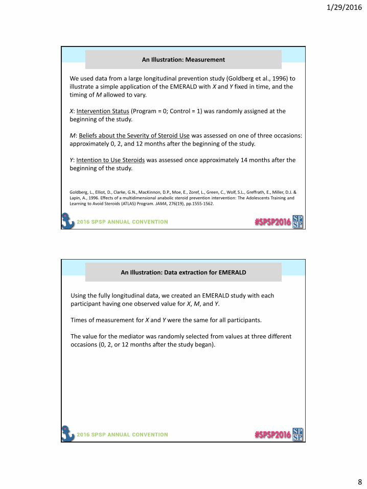
Judd et al.’s criteria to establish mediation
(1) Is there a difference between the two drugs types in participants’ willingness to buy?
(2) Is there a difference between the two drugs types in perceived hazardousness of the drug?
(3) Does the difference in perceived hazardousnesspredict the difference in willingness to buy?
(4) Does the difference in perceived hazardousness accountfor the difference in willingness to buy?
Analytical goal: Determine if perceived hazardousness of the drug is a mediator of the effect of the drug name complexity on willingness to purchase.
ID M1 Y1 M2 Y2
1 3.8 4.4 4.4 3.62 4.2 4.2 5.2 2.03 4.0 4.0 4.0 4.04 4.4 3.0 3.0 5.2. . . . .. . . . .. . . . .22 3.2 4.2 5.8 2.8
3.9 3.9 4.7 3.3
Simple Complex
Mean
Yes, by a paired samples t-test.
Yes, by a paired samples t-test.
Yes, by a regression analysis.
Yes, by a regression analysis. The difference in willingness to buy goes away when controlling for the difference in perceived hazardousness
Observations
(2) This method is squarely rooted in the causal steps tradition to mediation analysisthat has been much criticized. Compare it to the “Baron and Kenny” criteria:
(3) There is no explicit quantification of the indirect effect, but it is the indirect effectthat is the primary focus in 21st century mediation analysis.
• Is Y2 statistically different than Y1? This is like asking whether there is a total effect of X (drug came complexity) on Y (willingness to buy).
• Is M2 statistically different than M1? This is like asking whether X affects the mediator.
• Does difference in M significantly predict difference in Y? This is like asking whether themediator affects the outcome.
All these things can be “fixed” by recasting JK&McC in a more familiar path-analytic form.
• Is there still evidence of a difference in Y after accounting for the mediator? This is like asking whether the mediator completely or partially accounts for the effect of X on Y.
(1) It seems very foreign relative to path-analytic approaches that now dominatemediation analysis in the between-subjects case. Where’s the path analysis?

1/29/2016
14
In a path analytic mediation framework
Goal: Model the effect of the drug name complexity on willingness to buy, directly as well as indirectly through the effect of the drug name complexity on perceived hazardousness.
Where is X in the data?
Perceived hazardousness
Willingness to buy
M2 relative to M1
Y2 relative to Y1
Drug namecomplexity
ID M1 Y1 M2 Y2
1 3.8 4.4 4.4 3.62 4.2 4.2 5.2 2.03 4.0 4.0 4.0 4.04 4.4 3.0 3.0 5.2. . . . .. . . . .. . . . .22 3.2 4.2 5.8 2.8
3.9 3.9 4.7 3.3
Simple Complex
Mean
a b
c'X Y
M
M2 – M1 = a + e2
Y2 – Y1 = c' + b(M2 – M1) + b2(M2 + M1)* + e3
cYX
c = c' + ab
Y2 – Y1 = c + e1
Y2 – Y1
Y2 – Y1
M2 – M1
In a path analytic mediation framework
* mean centered
Y1 = willingness to buy (simple)Y2 = willingness to buy (complex)M1 = hazardousness (simple)M2 = hazardousness (complex)
ab = c – c'
Absent from thisdiagram are the errors and the mean centered sum of mediator values
Regression on just a constant.

1/29/2016
15
c' = -0.085X Y
M
c = -0.564YX
Y2 – Y1
Y2 – Y1
M2 – M1
In a path analytic mediation framework
a = 0.800 b = -0.598
c = c' + ab
c = -0.085 + (0.800)(-0.598) = -0.085 + -0.479 = -0.564
Direct effect Indirect effect Indirect effectDirect effect Total effect
In this form, it is clearthat the effect of Xpartitions into twocomponents direct and indirect in the usual way. We can conduct inferential tests on these estimates as in anymediation analysis.
Statistical inference for the indirect effect
What really matters in mediation analysis is the indirect effect ab. Some options include:
“Sobel” test:Z = ab/se(ab), with p or confidence interval calculated assuming ab is normally distributed. This is not recommended because the sampling distribution of ab is not normal.
Monte Carlo confidence intervalAssumes a normal sampling distribution of a and b individually, then simulates the samplingdistribution of the product using Monte Carlo methods. This method is available in between-subjects mediation analysis and easy to do with the right software.
Test of joint significanceAre both a and b statistically significant? This is what Judd, Kenny, and McClelland use. Wedon’t recommend this as it requires two tests rather than one, and no interval estimate isprovided.
Bootstrap confidence intervalA natural choice as it assumes nothing about the sampling distribution of ab, and this is already common in between-subjects mediation analysis and easy to do with the right software.
1/29/2016
16
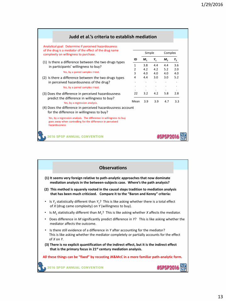
Implementation: Mplus, PROCESS, and MEMORE
MEMORE (MEdiation and MOderation for REpeated measures; pronounced like “memory”) is a bit easier to use than PROCESS for this kind of analysis but has PROCESS-like output. It is a new “macro” available for SPSS and SAS downloadable from www.afhayes.com and described for mediation problems in Montoya and Hayes (2015).
memore y=buy2 buy1/m=hazard2 hazard1/samples=10000.
%memore (data=drugname,y=buy2 buy1,m=hazard2 hazard1,samples=10000);
MEMORE
PROCESS
• Single and multiple mediator models. • Various inferential methods for indirect effects• Contrasts between indirect effects in multiple mediator models• Moderated mediation analysis functions coming soon.
SPSS:
SAS:
PROCESS for SPSS and SAS (www.processmacro.org) can do this. How so is described in Montoya and Hayes (2015). See the discussion there.
MPLUS
See handout or Montoya and Hayes (2015) for code and output.
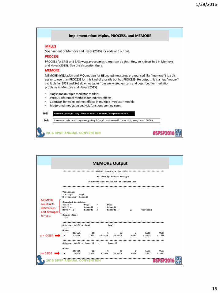
MEMORE Output
************************* MEMORE Procedure for SPSS ****************************
Written by Amanda Montoya
Documentation available at afhayes.com
********************************************************************************
Variables:
Y = buy2 buy1
M = hazard2 hazard1
Computed Variables:
Ydiff = buy2 - buy1
Mdiff = hazard2 - hazard1
Mavg = ( hazard2 + hazard1 ) /2 Centered
Sample Size:
22
********************************************************************************
Outcome: Ydiff = buy2 - buy1
Model
Effect SE t df p LLCI ULCI
'X' -.5636 .1932 -2.9168 21.0000 .0082 -.9655 -.1618
********************************************************************************
Outcome: Mdiff = hazard2 - hazard1
Model
Effect SE t df p LLCI ULCI
'X' .8000 .2579 3.1024 21.0000 .0054 .2637 1.3363
********************************************************************************
a = 0.800
c = -0.564
MEMOREconstructsdifferencesand averagesfor you.

1/29/2016
17
MEMORE Output
********************************************************************************
Outcome: Ydiff = buy2 - buy1
Model Summary
R R-sq MSE F df1 df2 p
.7721 .5961 .3667 14.0213 2.0000 19.0000 .0002
Model
coeff SE t df p LLCI ULCI
'X' -.0851 .1577 -.5399 19.0000 .5955 -.4152 .2449
Mdiff -.5981 .1131 -5.2869 19.0000 .0000 -.8349 -.3613
Mavg -.1818 .1683 -1.0803 19.0000 .2935 -.5341 .1705
********************** TOTAL, DIRECT, AND INDIRECT EFFECTS **********************
Total effect of X on Y
Effect SE t df p LLCI ULCI
-.5636 .1932 -2.9168 21.0000 .0082 -.9655 -.1618
Direct effect of X on Y
Effect SE t df p LLCI ULCI
-.0851 .1577 -.5399 19.0000 .5955 -.4152 .2449
Indirect Effect of X on Y through M
Effect BootSE BootLLCI BootULCI
Ind1 -.4785 .1363 -.7423 -.2063
Indirect Key
Ind1 X -> M1diff -> Ydiff
************************* ANALYSIS NOTES AND WARNINGS **************************
Bootstrap confidence interval method used: Percentile bootstrap.
Number of bootstrap samples for bootstrap confidence intervals: 10000
b = -0.598c' = -0.085
c' = -0.085
c = -0.564
ab with 95% bootstrapconfidence interval. This isconsistent with a claim ofmediation.

1/29/2016
18
Extension to multiple mediator models
A parallel multiple mediator model with k mediators A serial multiple mediator model with 2 mediators
Why do this?(1) More consistent with the complexity of real world-processes and theory.(2) Allows for the testing of competing theories through different processes, as
indirect effects can be formally compared.
An additional mediator measured in each condition
Data are still from Dohle, S., & Siegrist, M. (2014). Fluency of pharmaceutical drug names predicts perceived hazardousness, assumed side effects, and willingness to buy. Journal of Health Psychology, 19, 1241-1249.
Participants also evaluated how effective they thoughtthe drug would be.
M1. = Perceived hazardousness (1 to 7, higher = more)M2. = Perceived effectiveness (1 to 7, higher = more)Y = Willingness to purchase (1 to 7, higher = more)Measurement 1 = Average judgment about drugs
with simple namesMeasurement 2 = Average judgment about drugs
with complex name
Analytical goal: Is the effect of drug name complexity on willingness to purchase mediated by hazardousness? effectiveness? Both? Are the indirect effects the same or different?
M11 M21 Y1 M21 M22 Y2
3.8 4.2 4.4 4.4 4.0 3.64.2 4.4 4.2 5.2 3.6 2.04.0 4.0 4.0 4.0 4.0 4.04.4 4.2 3.0 3.0 4.8 5.2. . . . .. . . . .. . . . .3.2 4.6 4.2 5.8 5.6 2.8
3.9 4.4 3.9 4.7 4.1 3.3
Simple Complex
Mean

1/29/2016
19
X Y
M1
Y2 – Y1
M12 – M11
M2
M22 – M21
cYX
Y2 – Y1
A parallel mediation model in path analytic form
c'
M22 – M21 = a2 + e3
Y2 – Y1 = c' + b1(M12 – M11) + b2(M22 – M21) + b3(M12 + M11)* +b4(M22 + M21)* + e4
c = c' + a1b1+ a2b2
Y2 – Y1 = c + e1
M12 – M11 = a1 + e2
Absent from thisdiagram are the errors and the mean centered sum of mediator values
a1 b1
a2 b2
Y1 = willingness to buy (simple)Y2 = willingness to buy (complex)M11 = hazardousness (simple)M12 = hazardousness (complex)M21 = effectiveness (simple)M22 = effectiveness (complex)
* mean centered
X Y
M1
Y2 – Y1
M12 – M11
M2
M22 – M21
YX
Y2 – Y1
A parallel mediation model in path analytic form
Y1 = willingness to buy (simple)Y2 = willingness to buy (complex)M11 = hazardousness (simple)M12 = hazardousness (complex)M21 = effectiveness (simple)M22 = effectiveness (complex)
c' = -0.036
c = -0.564
a1 = 0.800 b1 = -0.591
a2 = -0.300 b2 = 0.185
c = -0.036 + (0.800)(-0.591) + (-0.300)(0.185) = -0.036 + -0.473 + -0.055 = -0.564
Direct effect Indirect effect via M1 Total effect
c = c' + a1b1+ a2b2
Indirect effect via M2 Direct effect Indirect effects

1/29/2016
20
X Y
M1
Y2 – Y1
M12 – M11
M2
Statistically comparing indirect effects
Y1 = willingness to buy (simple)Y2 = willingness to buy (complex)M11 = hazardousness (simple)M12 = hazardousness (complex)M21 = effectiveness (simple)M22 = effectiveness (complex)
a1 = 0.800 b1 = -0.591
a2 = -0.300 b2 = 0.185
M22 – M21
Specific indirect effect of name complexity through perceived hazardousness:
a1b1= (0.800)(-0.591) = -0.473
Specific indirect effect of name complexity through perceived effectiveness:
a2b2= (-0.300)(0.185) = -0.056
We can easily test whether these indirect effects are equal or different using bootstrapping.MEMORE for SPSS and SAS does this test.
Analytical goal: Determine if
the indirect effect of name
complexity on willingness to
buy through hazardousness is
different than the indirect effect
through effectiveness.
MEMORE Output
MEMORE can do all this, including bootstrap confidence intervals for specific indirect effects and their difference.
Variables:
Y = buy2 buy1
M1 = hazard2 hazard1
M2 = effect2 effect1
Computed Variables:
Ydiff = buy2 - buy1
M1diff = hazard2 - hazard1
M2diff = effect2 - effect1
M1avg = ( hazard2 + hazard1 ) /2 Centered
M2avg = ( effect2 + effect1 ) /2 Centered
Sample Size:
22
********************************************************************************
Outcome: Ydiff = buy2 - buy1
Model
Effect SE t df p LLCI ULCI
'X' -.5636 .1932 -2.9168 21.0000 .0082 -.9655 -.1618
********************************************************************************
Outcome: M1diff = hazard2 - hazard1
Model
Effect SE t df p LLCI ULCI
'X‘ .8000 .2579 3.1024 21.0000 .0054 .2637 1.3363
********************************************************************************
memore y=buy2 buy1/m=hazard2 hazard1 effect2 effect1/contrast=1/samples=10000.
%memore (data=drugname,y=buy2 buy1,m=hazard2 hazard1 effect2 effect1,contrast=1,samples=10000);
SPSS:
SAS:
c path
a1 path

1/29/2016
21
MEMORE Output
********************************************************************************
Outcome: M2diff = effect2 - effect1
Model
Effect SE t df p LLCI ULCI
'X' -.3000 .1798 -1.6683 21.0000 .1101 -.6740 -.0740
********************************************************************************
Outcome: Ydiff = buy2 - buy1
Model Summary
R R-sq MSE F df1 df2 p
.8212 .6744 .3304 8.8040 4.0000 17.0000 .0005
Model
coeff SE t df p LLCI ULCI
'X' -.0357 .1517 -.2352 17.0000 .8169 -.3557 .2844
M1diff -.5905 .1165 -5.0684 17.0000 .0001 -.8364 -.3447
M2diff .1851 .1596 1.1599 17.0000 .2621 -.1516 .5218
M1avg -.2898 .1738 -1.6679 17.0000 .1137 -.6564 .0768
M2avg -.2361 .1625 -1.4528 17.0000 .1645 -.5791 .1068
********************************************************************************
a2 path
b2 path
b1 path
c' path
MEMORE Output
********************** TOTAL, DIRECT, AND INDIRECT EFFECTS **********************
Total effect of X on Y
Effect SE t df p LLCI ULCI
-.5636 .1932 -2.9168 21.0000 .0082 -.9655 -.1618
Direct effect of X on Y
Effect SE t df p LLCI ULCI
-.0357 .1517 -.2352 17.0000 .8169 -.3557 .2844
Indirect Effect of X on Y through M
Effect BootSE BootLLCI BootULCI
Ind1 -.4724 .1469 -.7445 -.1644
Ind2 -.0555 .0964 -.2177 .1943
Total -.5280 .1411 -.7695 -.2173
Indirect Key
Ind1 X -> M1diff -> Ydiff
Ind2 X -> M2diff -> Ydiff
Pairwise Contrasts Between Specific Indirect Effects
Effect BootSE BootLLCI BootULCI
(C1) -.4169 .2045 -.8744 -.0178
Contrast Key:
(C1) Ind1 - Ind2
************************* ANALYSIS NOTES AND WARNINGS **************************
Bootstrap confidence interval method used: Percentile bootstrap.
Number of bootstrap samples for bootstrap confidence intervals: 10000
c path
a1b1
c' path
a2b2
a1b1 – a2b2 = -0.472 – -0.055 = -0.417
Point estimate and 95% bootstrap confidence interval for the difference between the two specific indirect effects. They are statistically different.
Point estimates and 95% bootstrap confidence intervals for the specific indirect effects. These areconsistent with a claim of mediation by hazardousness but not effectiveness.

1/29/2016
22
X Y
M1
Y2 – Y1
M12 – M11
M2
M22 – M21
cYX
Y2 – Y1
A serial mediation model in path analytic form
c'
M22 – M21 = a2 + a3(M12 – M11) + b5(M12 + M11)* + e3
Y2 – Y1 = c' + b1(M12 – M11) + b2(M22 – M21) + b3(M12 + M11)* +b4(M22 + M21)* + e4
c = c' + a1b 1+ a2b2 + a1a3b2
Y2 – Y1 = c + e1
M12 – M11 = a1 + e2
Absent from thisdiagram are the errors and the mean centered sum of mediator values
a1 b1
a2 b2
Y1 = willingness to buy (simple)Y2 = willingness to buy (complex)M11 = hazardousness (simple)M12 = hazardousness (complex)M21 = effectiveness (simple)M22 = effectiveness (complex)
* mean centered
a3
MEMORE Output
MEMORE can do all this, including bootstrap confidence intervals for specific indirect effects and their difference.
Variables:
Y = buy2 buy1
M1 = hazard2 hazard1
M2 = effect2 effect1
Computed Variables:
Ydiff = buy2 - buy1
M1diff = hazard2 - hazard1
M2diff = effect2 - effect1
M1avg = ( hazard2 + hazard1 ) /2 Centered
M2avg = ( effect2 + effect1 ) /2 Centered
Sample Size:
22
********************************************************************************
Outcome: Ydiff = buy2 - buy1
Model
Effect SE t df p LLCI ULCI
'X' -.5636 .1932 -2.9168 21.0000 .0082 -.9655 -.1618
********************************************************************************
Outcome: M1diff = hazard2 - hazard1
Model
Effect SE t df p LLCI ULCI
'X‘ .8000 .2579 3.1024 21.0000 .0054 .2637 1.3363
********************************************************************************
memore y=buy2 buy1/m=hazard2 hazard1 effect2 effect1/contrast=1/serial=1/samples=10000.
%memore (data=drugname,y=buy2 buy1,m=hazard2 hazard1 effect2 effect1,contrast=1,serial=1,samples=10000);
SPSS:
SAS:
c path
a1 path

1/29/2016
23
MEMORE Output
********************************************************************************
Outcome: M2diff = effect2 - effect1
Model Summary
R R-sq MSE F df1 df2 p
.3308 .1094 .7003 1.1675 2.0000 19.0000 .3325
Model
coeff SE t df p LLCI ULCI
'X' -.1224 .2179 -.5618 19.0000 .5808 -.5785 .3337
M1diff -.2220 .1563 -1.4200 19.0000 .1718 -.5493 .1052
M1avg .0411 .2326 .1766 19.0000 .8617 -.4457 .5278
********************************************************************************
Outcome: Ydiff = buy2 - buy1
Model Summary
R R-sq MSE F df1 df2 p
.8212 .6744 .3304 8.8040 4.0000 17.0000 .0005
Model
coeff SE t df p LLCI ULCI
'X' -.0357 .1517 -.2352 17.0000 .8169 -.3557 .2844
M1diff -.5905 .1165 -5.0684 17.0000 .0001 -.8364 -.3447
M2diff .1851 .1596 1.1599 17.0000 .2621 -.1516 .5218
M1avg -.2898 .1738 -1.6679 17.0000 .1137 -.6564 .0768
M2avg -.2361 .1625 -1.4528 17.0000 .1645 -.5791 .1068
a2 path
b2 path
b1 path
c' path
a3 path
MEMORE Output
********************** TOTAL, DIRECT, AND INDIRECT EFFECTS **********************
Total effect of X on Y
Effect SE t df p LLCI ULCI
-.5636 .1932 -2.9168 21.0000 .0082 -.9655 -.1618
Direct effect of X on Y
Effect SE t df p LLCI ULCI
-.0357 .1517 -.2352 17.0000 .8169 -.3557 .2844
Indirect Effect of X on Y through M
Effect BootSE BootLLCI BootULCI
Ind1 -.4724 .1469 -.7445 -.1644
Ind2 -.0227 .0611 -.1531 .1085
Ind3 -.0329 .0912 -.2401 .1499
Total -.5280 .1411 -.7695 -.2173
Indirect Key
Ind1 X -> M1diff -> Ydiff
Ind2 X -> M2diff -> Ydiff
Ind3 X -> M1diff -> M2diff -> Ydiff
Pairwise Contrasts Between Specific Indirect Effects
Effect BootSE BootLLCI BootULCI
(C1) -.4498 .1595 -.7649 -.1419
(C2) -.4396 .2033 -.8409 -.0256
(C3) .0102 .1209 -.2234 .2914
Contrast Key:
(C1) Ind1 - Ind2
(C2) Ind1 - Ind3
(C3) Ind2 - Ind3
************************* ANALYSIS NOTES AND WARNINGS **************************
c path
a1b1
c' path
a2b2
Point estimates and 95% bootstrap confidence intervals for the specific indirect effects. Theseresults are consistent with a claim of mediation by hazardousness alone but not effectiveness orhazardousness and effectiveness in serial.
a1b1 – a2b2 = -0.473 – -0.023 = -0.450
Point estimates and 95% bootstrap confidence intervals for the difference between pairs of specific indirect effects.
a2a3b2
a1b1 – a3b3 = -0.473 – -0.033 = -0.440a2b2 – a3b3 = -0.023 – -0.033 = 0.010

1/29/2016
24
Summary
• Framing Judd, Kenny and McClelland in a path-analytic framework allows for:• Focusing inference about mediation on the indirect effect• Use of modern inferential methods for the indirect effect (e.g., bootstrapping)• Easy generalization to parallel and serial multiple mediation models.
• PROCESS or MEMORE can be used to easily estimate simple mediation models, including a variety of options for inference.
• MEMORE can be used to estimate parallel and serial multiple mediation models, including many options for inference. • Researchers can compare theories about processes, by testing if indirect
effects through proposed mediators differ significantly.
• Easy to extend to conditional process models, where the indirect effect is moderated by some other variable . • Test for order effects, mixed designs (between and within-subject factors),
moderation by individual differences.
Thank you!
Thank you to Simone Dohle and Michael Siegrist for allowing us to use their data! Thanks to the National Science Foundation Graduate Research Fellowship and The Ohio State University Distinguished Dean’s University Fellowship for supporting Amanda Montoya.

1/29/2016
25
ACCURATE INDIRECT EFFECTS IN MULTILEVEL MEDIATION FOR REPEATED MEASURES DATA
Amanda Sharples and Elizabeth Page-GouldUniversity of Toronto
Mediator
OutcomePredictor
a b
c'
Indirect effect = a × bTotal effect = Indirect effect + c'
Mediation

1/29/2016
26
Participant 1
Observation Observation Observation
Participant 2
Observation Observation Observation
Nested (Repeated Measures) Data
Multilevel Models
Multilevel Mediation
Mediator
OutcomePredictor
a b
c'
Indirect effect = a × bTotal effect = Indirect effect + c'
1/29/2016
27
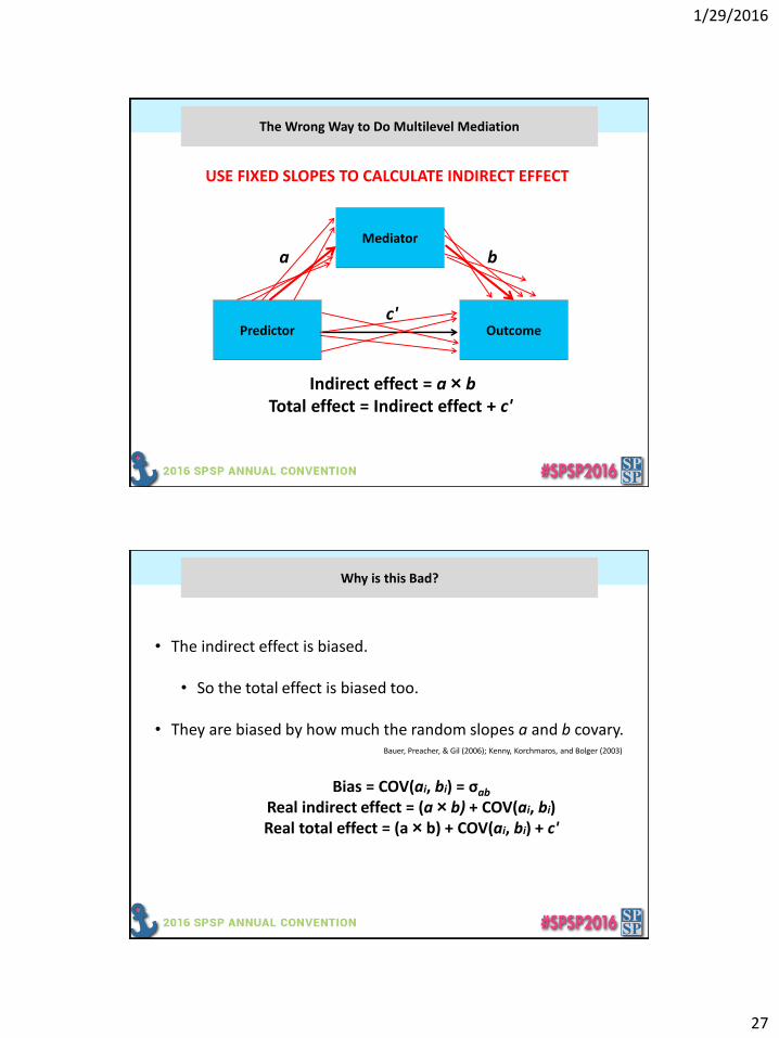
The Wrong Way to Do Multilevel Mediation
Mediator
OutcomePredictor
a b
c'
Indirect effect = a × bTotal effect = Indirect effect + c'
USE FIXED SLOPES TO CALCULATE INDIRECT EFFECT
Bauer, Preacher, & Gil (2006); Kenny, Korchmaros, and Bolger (2003)
Why is this Bad?
• The indirect effect is biased.
• So the total effect is biased too.
• They are biased by how much the random slopes a and b covary.
Bias = COV(ai, bi) = σab
Real indirect effect = (a × b) + COV(ai, bi) Real total effect = (a × b) + COV(ai, bi) + c'

1/29/2016
28
The Right Way to Do Multilevel Mediation
Mediator
OutcomePredictor
a b
c'
Indirect effect = Mean(ai × bi)Total effect = Mean(Indirect effecti + c'i)
TAKE RANDOM SLOPES INTO ACCOUNT
The Right Way to Do Multilevel Mediation
OutgroupSympathy
Outgroup Warmth
Group Membership
a b
c'
Indirect effect = Mean(ai × bi)Total effect = Mean(Indirect effecti + c'i)
TAKE RANDOM SLOPES INTO ACCOUNT
1/29/2016
29
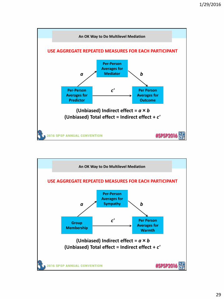
An OK Way to Do Multilevel Mediation
Per-Person Averages for
Mediator
Per Person Averages for
Outcome
Per-Person Averages for
Predictor
a b
c'
(Unbiased) Indirect effect = a × b(Unbiased) Total effect = Indirect effect + c'
USE AGGREGATE REPEATED MEASURES FOR EACH PARTICIPANT
An OK Way to Do Multilevel Mediation
Per-Person Averages for
Sympathy
Per Person Averages for
Warmth
Group Membership
a b
c'
(Unbiased) Indirect effect = a × b(Unbiased) Total effect = Indirect effect + c'
USE AGGREGATE REPEATED MEASURES FOR EACH PARTICIPANT

1/29/2016
30
How do we determine the robustness of our effects?
• There have been approaches put forward, but…
• Bootstrapping is ideal because• It does not require the assumption that the
random effects are normally distributed.• It is already ubiquitous in social psychology
(especially in mediation analysis)
14
1
6
7
10
5
2 9
Original SampleResample 1 Resample 2
Mediator
OutcomePredictor
a bc'
6
11
1
2
7
10
15 8 14
5
8
2
10
15
9 7
Bootstrapping for confidence intervals
Mediator
OutcomePredictor
a bc'
Mediator
OutcomePredictor
a bc'

1/29/2016
31
Goals of Current Demonstration
• Demonstrate how you can calculate unbiased indirect and total effects in multilevel mediation models.
• Demonstrate how you can use a bootstrappingapproach to estimate confidence intervals foryour effects.
Research Questions
• Will people rate their target in-group more warmlythan target outgroups?
• Can this be explained by greater sympathy towardthe target in-group (i.e., an indirect effect).

1/29/2016
32
Method: Sample
• N = 340 (community members)
• 62% female, 38% male
• Age range: 16-75
• Ethnicity: 33% White, 28% East Asian, 28% SouthAsian, 5% Black, 3% Arab, 2% Latino
Arabic BlackEast
AsianSouth Asian
First Nation
WhiteLatino
Method: Questionnaire
• Demographic information (e.g., ethnicity).
• Sympathy (0 = not at all sympathetic to 10 = verysympathetic) toward 7 target ethnic groups.
• Warmth (0 = cold to 10 = warm) toward 7 targetethnic groups.

1/29/2016
33
Arabic BlackEast
AsianSouth Asian
First Nation
WhiteLatino
Participant
Analytic Approach
Bootstrap Analysis in R:
• Created a function “indirect.mlm”
• Runs the relevant multilevel models in each resample
• Multiplies together the random a and b slopes and takes the mean of these products
• Use the “boot” package to do the multilevel mediation
Method: Questionnaire

1/29/2016
34
Within-Person Effects:• Unbiased Indirect effect = Mean(ai × bi)• Unbiased Total effect = Mean(Indirect effecti + c'i)
Between-Person Effects:• Indirect effect = a × b• Total effect = Indirect effect + c'
Analytic Approach
Analytic Approach
boot(data=data.set, R=1000,
strata=ID,
statistic=indirect.mlm,
y=“warmth”, x=“target”,
m=“sympathy”, group.id=“ID”,
between.m=T,
uncentered.x=F)

1/29/2016
35
-.594 [-.707, -.482].178 [.139, .214]within
.471 [.463, .520]between
-.601 [-.686, -.498]
Total effect = -.733 [-.823, -.643]
abwithin -.131 [-.180, -.103]abbetween -.280 [-.352, -.236]
Sympathy
Warmth
Group Membership
-1=in-group, 1 = outgroup
a b
c'
Results (unbiased)
-.594 [-.707, -.482].178 [.139, .214]within
.471 [.463, .520]between
-.601 [-.686, -.498]
Total effect = -.784 [-.871, -.696]
abwithin -.106 [-.138, -.176]abbetween -.280 [-.352, -.236]
Sympathy
Warmth
Group Membership
-1 = in-group, 1 = outgroup
a b
c'
Results (biased)

1/29/2016
36
Bias in indirect effect:
Biased: abwithin = -.106 [-.138, -.076]Unbiased: abwithin = -.131 [-.180, -.103]
Difference = .025 [.015, .058] = σab
Bauer et al. (2006)
Results
• Difference between biased and unbiased effects is equal to covariance between random slopes for paths a and b.
Bauer et al. (2006)
Bias in total effect:
Biased: c = -.784 [-.871, -.696]Unbiased: c = -.733 [-.823, -.643]
Difference = -.052 [-.086, -.020]
Bauer et al. (2006)
Results
• Difference between biased and unbiased total effect is equal to
abunbiased – abbiased + σab
Bauer et al. (2006)

1/29/2016
37
Discussion
• Download R script to run this analysis• www.page-gould.com/r/indirectmlm
• Currently, SPSS doesn’t allow you to save random slopes in its MIXED procedure• You can’t do this analysis in SPSS right now.• IBM says this is planned for future release.
• Good news!• We are creating a web application for non-R users.
Take Home Message
• Proof of concept• You can bootstrap indirect effects in multilevel
mediation analysis.
www.page-gould.com/r/indirectmlm
1/29/2016
38
Thank you!
Co-author:
Elizabeth Page-Gould
Lab and Research Assistants:
Social Psychophysiology and Quantitative Methods Lab (SPRQL)
Funding Sources:
Awarded to Sharples:
Ontario Graduate Scholarship
Awarded to Page-Gould:
Canada Research Chairs
Canada Foundation for Innovation
Connaught Fund New Researcher Award
Ontario Ministry of Research & Innovation
Social Sciences and Humanities Research Council (SSHRC) Insight Grants