Advanced Textbooks in Control and Signal Processing

Series Editors

Professor Michael J. Grimble, Professor of Industrial Systems and DirectorProfessor Michael A. Johnson, Professor Emeritus of Control Systems and Deputy Director

Industrial Control Centre, Department of Electronic and Electrical Engineering,University of Strathclyde, Graham Hills Building, 50 George Street, Glasgow G1 1QE, UK

Other titles published in this series:

Genetic AlgorithmsK.F. Man, K.S. Tang and S. Kwong

Neural Networks for Modelling and Control of Dynamic SystemsM. Nørgaard, O. Ravn, L.K. Hansen and N.K. Poulsen

Modelling and Control of Robot Manipulators (2nd Edition)L. Sciavicco and B. Siciliano

Fault Detection and Diagnosis in Industrial SystemsL.H. Chiang, E.L. Russell and R.D. Braatz

Soft ComputingL. Fortuna, G. Rizzotto, M. Lavorgna, G. Nunnari, M.G. Xibilia and R. Caponetto

Statistical Signal ProcessingT. Chonavel

Discrete-time Stochastic Processes (2nd Edition)T. Söderström

Parallel Computing for Real-time Signal Processing and ControlM.O. Tokhi, M.A. Hossain and M.H. Shaheed

Multivariable Control SystemsP. Albertos and A. Sala

Control Systems with Input and Output ConstraintsA.H. Glattfelder and W. Schaufelberger

Analysis and Control of Non-linear Process SystemsK. Hangos, J. Bokor and G. Szederkényi

Model Predictive Control (2nd Edition)E.F. Camacho and C. Bordons

Principles of Adaptive Filters and Self-learning SystemsA. Zaknich

Digital Self-tuning ControllersV. Bobál, J. Böhm, J. Fessl and J. Machácek

Control of Robot Manipulators in Joint SpaceR. Kelly, V. Santibáñez and A. Loría

Robust Control Design with MATLAB®D.-W. Gu, P.Hr. Petkov and M.M. Konstantinov

Active Noise and Vibration ControlM.O. TokhiPublication due September 2005

W.H. Kwon and S. Han

Receding HorizonControlModel Predictive Control for State Models

With 51 Figures

123

Wook Hyun Kwon, PhDSoohee Han, PhDSchool of Electrical Engineering and Computer ScienceSeoul National UniversitySan 56-1 Shinlim-dong Gwanak-kuSeoul 151-742Korea

British Library Cataloguing in Publication DataKwon, W. H. (Wook Hyun)

Receding horizon control: model predictive control forstate models. - (Advanced textbooks in control and signalprocessing)1. Predictive controlI. Title II. Han, S.629.8

ISBN-10: 1846280249

Library of Congress Control Number: 2005927907

Advanced Textbooks in Control and Signal Processing series ISSN 1439-2232ISBN-10: 1-84628-024-9 e-ISBN: 1-84628-017-6 Printed on acid-free paperISBN-13: 978-1-84628-024-5

© Springer-Verlag London Limited 2005

MATLAB® is the registered trademark of The MathWorks, Inc., 3 Apple Hill Drive Natick, MA 01760-2098, U.S.A. http://www.mathworks.com

Apart from any fair dealing for the purposes of research or private study, or criticism or review, aspermitted under the Copyright, Designs and Patents Act 1988, this publication may only be reproduced,stored or transmitted, in any form or by any means, with the prior permission in writing of thepublishers, or in the case of reprographic reproduction in accordance with the terms of licences issuedby the Copyright Licensing Agency. Enquiries concerning reproduction outside those terms should besent to the publishers.

The use of registered names, trademarks, etc. in this publication does not imply, even in the absence ofa specific statement, that such names are exempt from the relevant laws and regulations and thereforefree for general use.

The publisher makes no representation, express or implied, with regard to the accuracy of the infor-mation contained in this book and cannot accept any legal responsibility or liability for any errors oromissions that may be made.

Typesetting: Camera ready by authorsProduction: LE-TEX Jelonek, Schmidt & Vöckler GbR, Leipzig, GermanyPrinted in Germany

9 8 7 6 5 4 3 2 1

Springer Science+Business Mediaspringeronline.com

Dedicated to Allan and Myrna Pearson

Series Editors’ Foreword

The topics of control engineering and signal processing continue to flourish and develop. In common with general scientific investigation, new ideas, concepts and interpretations emerge quite spontaneously and these are then discussed, used, discarded or subsumed into the prevailing subject paradigm. Sometimes these innovative concepts coalesce into a new sub-discipline within the broad subject tapestry of control and signal processing. This preliminary battle between old and new usually takes place at conferences, through the Internet and in the journals of the discipline. After a little more maturity has been acquired by the new concepts then archival publication as a scientific or engineering monograph may occur.

A new concept in control and signal processing is known to have arrived when sufficient material has evolved for the topic to be taught as a specialised tutorial workshop or as a course to undergraduate, graduate or industrial engineers. Advanced Textbooks in Control and Signal Processing are designed as a vehicle for the systematic presentation of course material for both popular and innovative topics in the discipline. It is hoped that prospective authors will welcome the opportunity to publish a structured and systematic presentation of some of the newer emerging control and signal processing technologies in the textbook series.

In the 1970s many new control ideas were emerging. The optimal control paradigm initiated by the seminal papers of Kalman was growing into maturity For example, in 1971 the IEEE Transactions on Automatic Control published the famous special issue on LQG optimal control edited by Athans. The groundswell of ideas included finite-time optimal control solutions, and the concept of the separation principle partitioning solutions into control and estimation; these were influential concepts for later theorists. At the same time, the rapidly advancing power of digital control was being exploited by industry for the control of ever increasing numbers of process systems. Some control schemes of the 1970s were driven by the practical and commercial needs of industrial processes to operate within process regions bounded by constraints. Dynamic matrix control and model algorithmic control were typical software products that used models, cost functions and prediction to handle constrained industrial control problems.

The practical and theoretical experience of the 1970s finally produced generalised predictive control, model predictive control and the clear use of a receding horizon control principle as key methods for industrial control in the 1980s and 1990s. Today, model predictive control and the receding horizon

viii Series Editors’ Foreword

principle is the subject of a small but influential set of theoretical and practical textbooks.

Wook Hyun Kwon’s work on the receding horizon principle and model predictive control is grounded in the optimal control research of the late 1970s and has followed and contributed to the development of the field ever since. In this textbook, Professor Kwon and his colleague Soohee Han present their distinctive version of this important control methodology. The book can be used for a course study or for self study. Each chapter has a detailed problems section. MATLAB®

codes for various worked examples are given in an appendix so that the reader can try the various control and filter methods. Starred sections alert the reader and the lecturer to material that can be omitted if study time is constrained.

The opening chapter of the book succinctly reviews the concepts of receding horizon control and filters, the output feedback receding control problem and the use of prediction. A neat section on the advantages and disadvantages of the receding horizon control paradigm gives a useful insight into the reasons for the success of these methods. The most difficult task is then to construct a book framework for presenting material that has been evolving and developing since 1970s. The route planned by the authors is direct and effective. First, there is optimal control (Chapter 2). This covers the finite-time and infinite time horizon varieties for general systems, LQ, H-infinity, LQG and H2 optimal control. The chapter interleaves a section on Kalman and H-infinity filters as needed by the appropriate optimal control solutions. Chapter 3 introduces the receding horizon version of these optimal control formulations. A key feature of Chapter 3 is that state feedback is the active control mechanism. However, before moving to the challenging topic of output feedback receding horizon control, a chapter on receding horizon filtering is presented. The filters described in this Chapter 4 are used in the key results on output feedback receding horizon control. An important staging point of the textbook is Chapter 5 which presents detailed solutions to the important practical problem of output feedback receding horizon control. The exhaustive material of this chapter also includes a global optimization approach to the solution of the output feedback receding horizon control problem where a separation principle between control and estimation is proven. This is a highly satisfying outcome to the route taken so far by the authors. The final two chapters of the book then tackle the addition of constraints to the receding horizon control problem (Chapter 6) and receding horizon control with nonlinear dynamical process models (Chapter 7).

Overall, the textbook gives a well-structured presentation to receding horizon control methods using state-space models. The comprehensiveness of the presentation enables flexibility in selecting sections and topics to support an advanced course. The postgraduate student and the academic researcher will find many topics of interest for further research and contemplation in this fine addition to the series of advanced course textbooks in control and signal processing.

M.J. Grimble and M.A. Johnson Industrial Control Centre Glasgow, Scotland, U.K.

March 2005

Preface

This book introduces some essentials of receding horizon control (RHC) thathave been emerged as a successful feedback strategy in many industry fields,including process industries in particular. RHC is sometimes called receding-horizon predictive control (RHPC) and is better known as model predictivecontrol (MPC) for state-space models.

RHC is based on the conventional optimal control that is obtained byminimization or mini-maximization of some performance criterion either for afixed finite horizon or for an infinite horizon. RHC introduces a new concept ofthe receding horizon that is different from a fixed finite horizon and an infinitehorizon. The basic concept of RHC is as follows. At the current time, optimalcontrols, either open loop or closed loop, are obtained on a fixed finite horizonfrom the current time. Among the optimal controls on the fixed finite horizon,only the first one is implemented as the current control law. The procedureis then repeated at the next time with a fixed finite horizon from the nexttime. Owing to this unique characteristic, there are several advantages forwide acceptance of RHC, such as closed-loop structure, guaranteed stability,good tracking performance, input/output (I/O) constraint handling, simplecomputation, and easy extension to nonlinear systems.

Historically, generalized predictive control (GPC) and MPC has been in-vestigated and implemented for industrial applications independently. Origi-nally, RHC dealt with state-space models, while GPC and MPC dealt withI/O models. These three controls are equivalent to one another when the prob-lem formulation is the same. Since the recent problem formulations for theabove three predictive controls are based on state-space models, RHC basedon state-space models in this book will be useful in understanding the globalpicture of the predictive controls.

Discrete-time systems are discussed in this book, since they are useful formodern computer applications and they are easier to convey basic conceptscompared with continuous systems. Most results in this book for discrete-timesystems can be obtained for continuous-time systems. This book starts fromsimpler systems of linear systems without constraints and then moves to linear

x Preface

systems with constraints and to nonlinear systems for better understanding,although we can begin with nonlinear systems for generality. Both minimiza-tion and mini-maximization optimal problems are dealt with for completeness.Also, both state feedback and output feedback controls are dealt with if possi-ble. For output controls, a new type of receding horizon finite impulse response(FIR) filter that utilizes measurement data on the receding filter horizon isintroduced, which may be similar, in concept, to RHC. This filter is used asa state estimator and also as a part of the output feedback RHC.

In this book, optimal solutions of RHCs, the stability and the performanceof the closed-loop system, and robustness with respect to disturbances aredealt with. Robustness with respect to parameter uncertainties is not coveredin this book.

This book is organized as follows. After a brief introduction to conceptsand advantages of RHCs in Chapter 1, conventional optimal controls such asdynamic programming and the minimum principle for nonlinear systems andLQ, LQG, and H∞ controls for linear systems are introduced in Chapter 2,since RHCs are based on these conventional optimal controls. In Chapter 3,state feedback RHCs are investigated in depth. In Chapter 4, state estimatorssuch as receding horizon FIR filters are introduced as alternative filters toconventional filters, which have some connections with RHCs. In Chapter 5,output feedback RHCs will be introduced with a finite memory structure andan unbiased condition. In Chapter 6, RHCs are given for linear systems withinput and state constraints. In Chapter 7, RHCs for nonlinear systems areexplained. In Chapters 6 and 7, introductory topics are covered in this book.Some fundamental theories necessary for RHC are given in the appendices.Sections denoted by an asterisk can be skipped when a course cannot coverall the materials of the book.

In each chapter, we introduce references that help challenging readers ob-tain a detailed knowledge of related areas. We tried to include the importantliterature, but this may not be complete. If we have missed citing some im-portant references, we sincerely apologize for that.

The first author appreciates the constant support of Allan and MyrnaPearson and Thomas Kailath since he was at Brown University as a graduatestudent and at Stanford University as a visiting professor respectively. Wewould like to express our appreciation to Ki back Kim, Young Sam Lee, andYoung Il Lee who finished their Ph.Ds at our laboratory and provided someinput to this book. Also, Choon Ki Ahn, Zhong Hua Quan, Bo Kyu Kwon,Jung Hun Park, and some other graduate students were of great help to us indeveloping this book.

Seoul, Korea Wook Hyun KwonJanuary 2005 Soohee Han

Contents

1 Introduction . . . . . . . . . . . . . . . . . . . . . . . . . . . . . . . . . . . . . . . . . . . . . . . 11.1 Control Systems . . . . . . . . . . . . . . . . . . . . . . . . . . . . . . . . . . . . . . . . . 11.2 Concept of Receding Horizon Controls . . . . . . . . . . . . . . . . . . . . . 31.3 Receding Horizon Filters and Output Feedback Receding

Horizon Controls. . . . . . . . . . . . . . . . . . . . . . . . . . . . . . . . . . . . . . . . . . . 71.4 Predictive Controls . . . . . . . . . . . . . . . . . . . . . . . . . . . . . . . . . . . . . . 81.5 Advantages of Receding Horizon Controls . . . . . . . . . . . . . . . . . . 91.6 About This Book . . . . . . . . . . . . . . . . . . . . . . . . . . . . . . . . . . . . . . . . 111.7 References . . . . . . . . . . . . . . . . . . . . . . . . . . . . . . . . . . . . . . . . . . . . . . 15

2 Optimal Controls on Finite and Infinite Horizons: A Review 172.1 Introduction . . . . . . . . . . . . . . . . . . . . . . . . . . . . . . . . . . . . . . . . . . . . 172.2 Optimal Control for General Systems . . . . . . . . . . . . . . . . . . . . . . 18

2.2.1 Optimal Control Based on Minimum Criterion . . . . . . . . 182.2.2 Optimal Control Based on Minimax Criterion . . . . . . . . . 24

2.3 Linear Optimal Control with State Feedback . . . . . . . . . . . . . . . . 262.3.1 Linear Quadratic Controls Based on Minimum

Criterion . . . . . . . . . . . . . . . . . . . . . . . . . . . . . . . . . . . . . . . . 262.3.2 H∞ Control Based on Minimax Criterion . . . . . . . . . . . . . 42

2.4 Optimal Filters . . . . . . . . . . . . . . . . . . . . . . . . . . . . . . . . . . . . . . . . . 492.4.1 Kalman Filter on Minimum Criterion . . . . . . . . . . . . . . . 492.4.2 H∞ Filter on Minimax Criterion . . . . . . . . . . . . . . . . . . . . 522.4.3 Kalman Filters on Minimax Criterion . . . . . . . . . . . . . . . . 56

2.5 Output Feedback Optimal Control . . . . . . . . . . . . . . . . . . . . . . . . . 572.5.1 Linear Quadratic Gaussian Control on Minimum

Criterion . . . . . . . . . . . . . . . . . . . . . . . . . . . . . . . . . . . . . . . . . 582.5.2 Output Feedback H∞ Control on Minimax Criterion . . . 61

2.6 Linear Optimal Controls via Linear Matrix Inequality . . . . . . . 662.6.1 Infinite Horizon Linear Quadratic Control via Linear

Matrix Inequality . . . . . . . . . . . . . . . . . . . . . . . . . . . . . . . . . 66

xii Contents

2.6.2 Infinite Horizon H∞ Control via Linear MatrixInequality . . . . . . . . . . . . . . . . . . . . . . . . . . . . . . . . . . . . . . . . 68

2.7 ∗ H2 Controls . . . . . . . . . . . . . . . . . . . . . . . . . . . . . . . . . . . . . . . . . . . . 702.8 References . . . . . . . . . . . . . . . . . . . . . . . . . . . . . . . . . . . . . . . . . . . . . . 742.9 Problems . . . . . . . . . . . . . . . . . . . . . . . . . . . . . . . . . . . . . . . . . . . . . . . 76

3 State Feedback Receding Horizon Controls . . . . . . . . . . . . . . . . 833.1 Introduction . . . . . . . . . . . . . . . . . . . . . . . . . . . . . . . . . . . . . . . . . . . . 833.2 Receding Horizon Controls in Predictive Forms . . . . . . . . . . . . . . 84

3.2.1 Predictive Forms . . . . . . . . . . . . . . . . . . . . . . . . . . . . . . . . . . 843.2.2 Performance Criteria in Predictive Forms . . . . . . . . . . . . . 85

3.3 Receding Horizon Control Based on Minimum Criteria . . . . . . . 873.3.1 Receding Horizon Linear Quadratic Control . . . . . . . . . . 873.3.2 Simple Notation for Time-invariant Systems . . . . . . . . . . 913.3.3 Monotonicity of the Optimal Cost . . . . . . . . . . . . . . . . . . . 953.3.4 Stability of Receding Horizon Linear Quadratic

Control . . . . . . . . . . . . . . . . . . . . . . . . . . . . . . . . . . . . . . . . 1043.3.5 Additional Properties of Receding Horizon Linear

Quadratic Control . . . . . . . . . . . . . . . . . . . . . . . . . . . . . . . . . 1153.3.6 A Special Case of Input–Output Systems . . . . . . . . . . . . . 122

3.4 Receding Horizon Control Based on Minimax Criteria . . . . . . . . 1253.4.1 Receding Horizon H∞ Control . . . . . . . . . . . . . . . . . . . . . . 1253.4.2 Monotonicity of the Saddle-point Optimal Cost . . . . . . . 1283.4.3 Stability of Receding Horizon H∞ Control . . . . . . . . . . . . 1333.4.4 Additional Properties . . . . . . . . . . . . . . . . . . . . . . . . . . . . . . 138

3.5 Receding Horizon Control via Linear Matrix Inequality Forms . 1393.5.1 Computation of Cost Monotonicity Condition . . . . . . . . . 1393.5.2 Receding Horizon Linear Quadratic Control via Batch

and Linear Matrix Inequality Forms . . . . . . . . . . . . . . . . . 1433.5.3 Receding Horizon H∞ Control via Batch and Linear

Matrix Inequality Forms . . . . . . . . . . . . . . . . . . . . . . . . . . . 1483.6 References . . . . . . . . . . . . . . . . . . . . . . . . . . . . . . . . . . . . . . . . . . . . . . 1503.7 Problems . . . . . . . . . . . . . . . . . . . . . . . . . . . . . . . . . . . . . . . . . . . . . . . 151

4 Receding Horizon Filters . . . . . . . . . . . . . . . . . . . . . . . . . . . . . . . . . . 1594.1 Introduction . . . . . . . . . . . . . . . . . . . . . . . . . . . . . . . . . . . . . . . . . . . . 1594.2 Dual Infinite Impulse Response Filter Based on Minimum

Criterion . . . . . . . . . . . . . . . . . . . . . . . . . . . . . . . . . . . . . . . . . . . . . . . 1614.3 Optimal Finite Impulse Response Filters Based on Minimum

Criterion . . . . . . . . . . . . . . . . . . . . . . . . . . . . . . . . . . . . . . . . . . . . . . 1654.3.1 Linear Unbiased Finite Impulse Response Filters . . . . . . 1654.3.2 Minimum Variance Finite Impulse Response Filters

with Nonsingular A . . . . . . . . . . . . . . . . . . . . . . . . . . . . . . . . 1674.3.3 Minimum Variance Finite Impulse Response Filters

with General A . . . . . . . . . . . . . . . . . . . . . . . . . . . . . . . . . . . 177

Contents xiii

4.3.4 Numerical Examples for Minimum Variance FiniteImpulse Response Filters . . . . . . . . . . . . . . . . . . . . . . . . . . . 188

4.4 Dual Infinite Impulse Response Filters Based on MinimaxCriterion . . . . . . . . . . . . . . . . . . . . . . . . . . . . . . . . . . . . . . . . . . . . . . . 190

4.5 Finite Impulse Response Filters Based on MinimaxCriterion . . . . . . . . . . . . . . . . . . . . . . . . . . . . . . . . . . . . . . . . . . . . 1954.5.1 Linear Unbiased Finite Impulse Response Filters . . . . . . 1954.5.2 L2-E Finite Impulse Response Filters . . . . . . . . . . . . . . . . 1974.5.3 H∞ Finite Impulse Response Filter . . . . . . . . . . . . . . . . . 2024.5.4 ∗ H2/H∞ Finite Impulse Response Filters . . . . . . . . . . . . . 204

4.6 References . . . . . . . . . . . . . . . . . . . . . . . . . . . . . . . . . . . . . . . . . . . . . . 2074.7 Problems . . . . . . . . . . . . . . . . . . . . . . . . . . . . . . . . . . . . . . . . . . . . . . . 209

5 Output Feedback Receding Horizon Controls . . . . . . . . . . . . . 2175.1 Introduction . . . . . . . . . . . . . . . . . . . . . . . . . . . . . . . . . . . . . . . . . . . . 2175.2 State-observer-based Output Feedback Controls . . . . . . . . . . . . . 2185.3 Predictor-based Output Feedback Controls . . . . . . . . . . . . . . . . . 2205.4 A Special Case of Input–Output Systems of General

Predictive Control . . . . . . . . . . . . . . . . . . . . . . . . . . . . . . . . . . . . . . . 2225.5 Finite Memory Control Based on Minimum Criterion . . . . . . . . 227

5.5.1 Finite Memory Control and Unbiased Condition . . . . . . . 2275.5.2 Linear Quadratic Finite Memory Control . . . . . . . . . . . . . 2305.5.3 ∗ Linear Quadratic Finite Memory Control with

General A . . . . . . . . . . . . . . . . . . . . . . . . . . . . . . . . . . . . . . . 2355.5.4 Properties of Linear Quadratic Finite Memory

Control . . . . . . . . . . . . . . . . . . . . . . . . . . . . . . . . . . . . . . . . 2395.6 Finite Memory Control Based on Minimax Criterion . . . . . . . . 244

5.6.1 Finite Memory Control and Unbiased Condition . . . . . . . 2445.6.2 L2-E Finite Memory Controls . . . . . . . . . . . . . . . . . . . . . . 2455.6.3 H∞ Finite Memory Controls . . . . . . . . . . . . . . . . . . . . . . . 2505.6.4 ∗ H2/H∞ Finite Memory Controls . . . . . . . . . . . . . . . . . . . . 254

5.7 References . . . . . . . . . . . . . . . . . . . . . . . . . . . . . . . . . . . . . . . . . . . . . . 2565.8 Problems . . . . . . . . . . . . . . . . . . . . . . . . . . . . . . . . . . . . . . . . . . . . . . . 256

6 Constrained Receding Horizon Controls . . . . . . . . . . . . . . . . . . . 2616.1 Introduction . . . . . . . . . . . . . . . . . . . . . . . . . . . . . . . . . . . . . . . . . . . . 2616.2 Reachable and Maximal Output Admissible Sets . . . . . . . . . . . . 2626.3 Constrained Receding Horizon Control with Terminal

Equality Constraint. . . . . . . . . . . . . . . . . . . . . . . . . . . . . . . . . . . . . . . . 2696.4 Constrained Receding Horizon Control with Terminal Set

Constraint . . . . . . . . . . . . . . . . . . . . . . . . . . . . . . . . . . . . . . . . . . . . . . 2726.5 Constrained Receding Horizon Control with Free Terminal

Cost . . . . . . . . . . . . . . . . . . . . . . . . . . . . . . . . . . . . . . . . . . . . . . . . . . 2776.6 Constrained Receding Horizon Control with Mixed

Constraints . . . . . . . . . . . . . . . . . . . . . . . . . . . . . . . . . . . . . . . . . . . 284

xiv Contents

6.7 Constrained Output Feedback Receding Horizon Control . . . . . 2866.8 References . . . . . . . . . . . . . . . . . . . . . . . . . . . . . . . . . . . . . . . . . . . . . . 2896.9 Problems . . . . . . . . . . . . . . . . . . . . . . . . . . . . . . . . . . . . . . . . . . . . . . . 290

7 Nonlinear Receding Horizon Controls . . . . . . . . . . . . . . . . . . . . . . 2977.1 Introduction . . . . . . . . . . . . . . . . . . . . . . . . . . . . . . . . . . . . . . . . . . . . 2977.2 Nonlinear Receding Horizon Control with Terminal Equality

Constraint . . . . . . . . . . . . . . . . . . . . . . . . . . . . . . . . . . . . . . . . . . . . . . 2987.3 Nonlinear Receding Horizon Control with Terminal Set

Constraints . . . . . . . . . . . . . . . . . . . . . . . . . . . . . . . . . . . . . . . . . . . . . 3007.4 Nonlinear Receding Horizon Control with Free Terminal Cost . 3047.5 Nonlinear Receding Horizon Control with Infinite Cost

Horizon . . . . . . . . . . . . . . . . . . . . . . . . . . . . . . . . . . . . . . . . . . . . . . . 3117.6 Nonlinear Receding Horizon Minimax Control with Free

Terminal Cost . . . . . . . . . . . . . . . . . . . . . . . . . . . . . . . . . . . . . . . . . . 3137.7 References . . . . . . . . . . . . . . . . . . . . . . . . . . . . . . . . . . . . . . . . . . . . . . 3167.8 Problems . . . . . . . . . . . . . . . . . . . . . . . . . . . . . . . . . . . . . . . . . . . . . . . 316

A Matrix Equality and Matrix Calculus . . . . . . . . . . . . . . . . . . . . . . 323A.1 Useful Inversion Formulae . . . . . . . . . . . . . . . . . . . . . . . . . . . . . . . . 323A.2 Matrix Calculus . . . . . . . . . . . . . . . . . . . . . . . . . . . . . . . . . . . . . . . . . 325

B System Theory . . . . . . . . . . . . . . . . . . . . . . . . . . . . . . . . . . . . . . . . . . . . 327B.1 Controllability and Observability . . . . . . . . . . . . . . . . . . . . . . . . . . 327B.2 Stability Theory . . . . . . . . . . . . . . . . . . . . . . . . . . . . . . . . . . . . . . . . . 330B.3 Lyapunov and Riccati Matrix Equations . . . . . . . . . . . . . . . . . . . . 331

C Random Variables . . . . . . . . . . . . . . . . . . . . . . . . . . . . . . . . . . . . . . . . 335C.1 Random Variables . . . . . . . . . . . . . . . . . . . . . . . . . . . . . . . . . . . . . . 335C.2 Gaussian Random Variable . . . . . . . . . . . . . . . . . . . . . . . . . . . . . . 336C.3 Random Process . . . . . . . . . . . . . . . . . . . . . . . . . . . . . . . . . . . . . . . . 339

D Linear Matrix Inequalities and Semidefinite Programming . 341D.1 Linear Matrix Inequalities . . . . . . . . . . . . . . . . . . . . . . . . . . . . . . . . 341D.2 Semidefinite Programming . . . . . . . . . . . . . . . . . . . . . . . . . . . . . . . . 343

E Survey on Applications . . . . . . . . . . . . . . . . . . . . . . . . . . . . . . . . . . . . 347

F MATLAB Programs . . . . . . . . . . . . . . . . . . . . . . . . . . . . . . . . . . . . . 349

References . . . . . . . . . . . . . . . . . . . . . . . . . . . . . . . . . . . . . . . . . . . . . . . . . . . . . 367

Index . . . . . . . . . . . . . . . . . . . . . . . . . . . . . . . . . . . . . . . . . . . . . . . . . . . . . . . . . . 375

1

Introduction

1.1 Control Systems

In this section, we will briefly discuss important topics for control systems,such as models, control objectives, control structure, and performance critera.

Models

The basic variables of dynamical control systems are input, state, and outputvariables that consist of controlled outputs and measured outputs, as in Fig-ure 1.1. The input variable is the control variable and the measured output isused for feedback. Usually, output variables are a subset of whole state vari-ables. In dynamical control systems, there can be several undesirable elements,such as disturbances, noises, nonlinear elements, time-delay, uncertainties ofdynamics and its parameters, constraints in input and state variables, etc.All or some parts of undesirable elements exist in each system, depending onthe system characteristics. A model can be represented as a stochastic systemwith noises or a deterministic system with disturbances. A model can be alinear or nonlinear system. Usually, dynamic models are described by state-space systems, but sometimes with input and output models.

Fig. 1.1. Control systems

2 1 Introduction

Control Objectives

There can be several objectives for control systems. The control is designedsuch that the controlled output tracks the reference signal under the aboveundesirable elements. Actually, the closed-loop stability and the tracking per-formance even under the undesirable elements are known to be importantcontrol objectives.

In order to achieve control objectives easily, the real system is separatedinto a nominal system without model uncertainties and an additional un-certain system representing the above undesirable elements. The control canbe designed first for the nominal system and then for the uncertain system.In this case, the control objectives can be divided into simpler intermediatecontrol objectives, such as

• Nominal stability: closed-loop stability for nominal systems.• Nominal performance: tracking performance for nominal systems.• Robust stability: closed-loop stability for uncertain systems (robust sta-

bility).• Robust performance: tracking performance for uncertain systems (robust

tracking performance).

The first three are considered to be the most important.

Control Structure

If all the states are measured we can use state feedback controls such asin Figure 1.2 (a). However, if only the outputs can be measured, then we haveto use output feedback controls such as in Figure 1.2 (b).

The state feedback controls are easier to design than the output feedbackcontrols, since state variables contain all the system information. Static feed-back controls are simpler in structure than dynamic feedback controls, butmay exist in limited cases. They are often used for state feedback controls.Dynamic feedback controls are easier to design than static feedback controls,but the dimension of the overall systems increases. They are often used foroutput feedback controls. Finite memory feedback controls, or simply finitememory controls, which are linear combinations of finite measured inputs andoutputs, can be another option, which will be explained extensively in thisbook later. The feedback control is required to be linear or allowed to be non-linear.

Performance Criterion

There are several approaches for control designs to meet control objectives.Optimal control has been one of the widely used methods. An optimal controlis obtained by minimizing or maximizing a certain performance criterion. It isalso obtained by mini-maximizing or maxi-minimizing a certain performance

1.2 Concept of Receding Horizon Controls 3

(a) State feedback control

(b) Output feedback control

Fig. 1.2. Feedback controls

criterion. Optimal controls are given on the finite horizon and also on the infi-nite horizon. For linear systems, popular optimal controls based on minimizingare the LQ controls for state feedback controls and the LQG controls for out-put feedback controls. Popular optimal controls based on mini-maximizing areH∞ controls.

The optimal controls are often given in open-loop controls for nonlinearsystems. However, optimal controls for linear systems often lead to feedbackcontrols. Therefore, special care should be taken to obtain a closed-loop controlfor nonlinear systems.

Even if optimal controls are obtained by satisfying some performance cri-teria, they need to meet the above-mentioned control objectives: closed-loopstability, tracking performance, robust stability, and robust tracking perfor-mance. Closed-loop optimal controls on the infinite horizon tend to meet thetracking performance and the closed-loop stability under some conditions.However, it is not so easy to achieve robust stability with respect to modeluncertainties.

Models, control structure, and performance criteria can be summarizedvisually in Figure 1.3.

1.2 Concept of Receding Horizon Controls

In conventional optimal controls, either finite horizons or infinite horizons aredealt with. Often, feedback control systems must run for a sufficiently longperiod, as in electrical power generation plants and chemical processes. Inthese ongoing processes, finite horizon optimal controls cannot be adopted, but

4 1 Introduction

Fig. 1.3. Components of control systems

infinite horizon optimal controls must be used. In addition, we can introducea new type of control, RHC that is based on optimal control.

The basic concept of RHC is as follows. At the current time, the optimalcontrol is obtained, either closed-loop type, or open-loop type, on a finitefixed horizon from the current time k, say [k, k + N ]. Among the optimalcontrols on the entire fixed horizon [k, k + N ], only the first one is adopted asthe current control law. The procedure is then repeated at the next time, say[k+1, k+1+N ]. The term “receding horizon” is introduced, since the horizonrecedes as time proceeds. There is another type of control, i.e. intervalwiseRHC, that will be explained later.

The concept of RHC can be easily explained by using a company’s invest-ment planning to maximize the profit. The investment planning should becontinued for the years to come as in feedback control systems. There couldbe three policies for a company’s investment planning:

(1) One-time long-term planningInvestment planning can be carried over a fairly long period, which is closer

to infinity, as in Figure 1.4. This policy corresponds to the infinite horizon op-timal control obtained over [k,∞].

(2) Periodic short-term planningInstead of the one-time long-term planning, we can repeat short-term in-

vestment planning, say investment planning every 5-years, which is given inFigure 1.5.

(3) Annual short-term planning

1.2 Concept of Receding Horizon Controls 5

2000 2001 2010

1st 5 years planning

2000 2001 2010

1st 5 years planning

Fig. 1.4. One-time long-term planning

2000 2001 2004

2005 2006 2009

2010 2011 2014

2000 2001 2004

2005 2006 2009

2010 2011 2014

Fig. 1.5. Periodic short-term planning

2000 2001 2004

2001 2002 2005

2009 2010 2013

2010 2011 2014

2000 2001 2009 2010

2000 2001 2004

2001 2002 2005

2009 2010 2013

2010 2011 2014

2000 2001 2009 2010

Fig. 1.6. Annual short-term planning

6 1 Introduction

For a new policy, it may be good to have a short-term planning every yearand the first year’s investment is selected for the current year’s investmentpolicy. This concept is depicted in Figure 1.6.

Now, which investment planning looks the best? Obviously we must deter-mine the definition of the “best”. The meaning of the “best” is very subjectiveand can be different depending on the individual. Among investment plan-nings, any one can be the best policy, depending on the perception of eachperson. The above question, about which investment planning is the best,was asked of students in a class without explaining many details. An averageseven or eight out of ten persons selected the third policy, i.e. annual short-term planning, as the best investment planning. This indicates that annualshort-term planning can have significant meanings.

The above examples are somewhat vague in a mathematical sense, butare adequate to explain the concepts of RHC. An annual short-term planningis exactly the same as RHC. Therefore, RHC may have significant meaningsthat will be clearer in the coming chapters. The periodic short-term investmentplanning in Figure 1.5 corresponds to intervalwise RHC. The term “interval-wise receding horizon” is introduced since the horizon recedes intervalwiseor periodically as time proceeds. Different types of investment planning arecompared with the different types of optimal control in Table 1.1. It is notedthat the short-term investment planning corresponds to finite horizon control,which works for finite time processes such as missile control systems.

Table 1.1. Investment planning vs control

Process Planning ControlOngoing process One-time long-term planning Infinite horizon control

Periodic short-term planning Intervalwise RHCAnnual short-term planning Receding horizon control

Finite time process Short-term planning Finite horizon control

There are several advantages to RHCs, as seen in Section 1.5. We takean example such as the closed-loop structure. Optimal controls for generalsystems are usually open-loop controls depending on the initial state. In thecase of infinite horizon optimal controls, all controls are open-loop controlsexcept the initial time. In the case of intervalwise RHCs, only the first controlon each horizon is a closed-loop control and others are open-loop controls. Inthe case of the RHCs, we always have closed-loop controls due to the repeatedcomputation and the implementation of only the first control.

1.3 Receding Horizon Filters and Output Feedback Receding Horizon Controls 7

1.3 Receding Horizon Filters and Output FeedbackReceding Horizon Controls

RHC is usually represented by a state feedback control if states are available.However, full states may not be available, since measurement of all statesmay be expensive or impossible. From measured inputs and outputs, we canconstruct or estimate all states. This is often called a filter for stochasticsystems or a state observer for deterministic systems. Often, it is called afilter for both systems. The well-known Luenberger observer for deterministicstate-space signal models and the Kalman filter for stochastic state-spacesignal models are infinite impulse response (IIR) type filters. This means thatthe state observer utilizes all the measured data up to the current time k fromthe initial time k0.

Instead, we can utilize the measured data on the recent finite time [k −Nf , k] and obtain an estimated state by a linear combination of the measuredinputs and outputs over the receding finite horizon with some weighting gainsto be chosen so that the error between the real state and the estimated oneis minimized. Nf is called the filter horizon size and is a design parameter.We will call this filter as the receding horizon filter. This is an FIR-typefilter. This concept is depicted in Figure 1.7. It is noted that in the signal

Fig. 1.7. Receding horizon filter

processing area the FIR filter has been widely used for unmodelled signalsdue to its many good properties, such as guaranteed stability, linear phase(zero error), robustness to temporary parameter changes and round-off error,etc. We can also expect such good properties for the receding horizon filters.

An output feedback RHC can be made by blind combination of a statefeedback RHC with a receding horizon filter, just like a combination of an LQ

8 1 Introduction

regulator and a Kalman filter. However, we can obtain an output feedbackRHC by an optimal approach, not by a blind combination. The output feed-back RHC is obtained as a linear combination of the measured inputs andoutputs over the receding finite horizon with some weighting gains to be cho-sen so that the given performance criterion is optimized. This control will becalled a receding horizon finite memory control (FMC). The above approachis comparable to the well-known LQG problem, where the control is assumedto be a function of all the measured inputs and outputs from the initial time.The receding horizon FMC are believed to have properties that are as goodas the receding horizon FIR filters and state feedback RHCs.

1.4 Predictive Controls

An RHC is one type of predictive control. There are two other well-knownpredictive controls, generalized predictive control (GPC) and model predictivecontrol (MPC). Originally, these three control strategies had been investigatedindependently.

GPC was developed in the self-tuning and adaptive control area. Somecontrol strategies that achieve minimum variance were adopted in the self-tuning control [AW73] [CG79]. The general frame work for GPC was suggestedby Clark et al. [CMT87]. GPC is based on the single input and single output(SISO) models such as auto regressive moving average (ARMA) or controlledauto regressive integrated moving average (CARIMA) models which have beenwidely used for most adaptive controls.

MPC has been developed on a model basis in the process industry area asan alternative algorithm to the conventional proportional integrate derivative(PID) control that does not utilize the model. The original version of MPCwas developed for truncated I/O models, such as FIR models or finite stepresponse (FSR) models. Model algorithmic control (MAC) was developed forFIR models [RRTP78] and the dynamic matrix control (DMC) was devel-oped for FSR models [CR80]. These two control strategies coped with I/Oconstraints. Since I/O models such as the FIR model or the FSR model arephysically intuitive, they are widely accepted in the process industry. How-ever, these early control strategies were somewhat heuristic, limited to theFIR or the FSR models, and not applicable to unstable systems. Thereafter,lots of extensions have been made for state-space models, as shown in surveypapers listed in Section 1.7.

RHC has been developed in academia as an alternative control to the cele-brated LQ controls. RHC is based on the state-space framework. The stabiliz-ing property of RHC has been shown for case of both continuous and discretesystems using the terminal equality constraint [KP77a] [KP77c]. Thereafter,it has been extended to tracking controls, output feedback controls, and non-linear controls [KG88] [MM90]. The state and input constraints were not con-

1.5 Advantages of Receding Horizon Controls 9

sidered in the early developments, but dealt in later works, as seen in theabove-mentioned survey papers.

The term “predictive” appears in GPC since the minimum variance isgiven in predicted values on the finite future time. The term “predictive”appears in MPC since the performance is given in predictive values on thefinite future time that can be computed by using the model. The performancefor RHC is the same as one for MPC. Thus, the term “predictive” can beincorporated in RHC as receding horizon predictive control (RHPC).

Since I/O models on which GPC and the early MPC are based can berepresented in state-space frameworks, GPC and the early MPC can be ob-tained from predictive controls based on state-space models. In this book, thepredictive controls based on the state space model will be dealt with in termsof RHC instead of MPC although MPC based on the state-space model is thesame as RHC.

1.5 Advantages of Receding Horizon Controls

RHC has made a significant impact on industrial control engineering andis being increasingly applied in process controls. In addition to industrialapplications, RHC has been considered to be a successful control theory inacademia. In order to exploit the reasons for such a preference, we may sum-marize several advantages of RHC over other existing controls.

• Applicability to a broad class of systems. The optimization problem overthe finite horizon, on which RHC is based, can be applied to a broadclass of systems, including nonlinear systems and time-delayed systems.Analytical or numerical solutions often exist for such systems.

• Systematic approach to obtain a closed loop control. While optimal con-trols for linear systems with input and output constraints or nonlinearsystems are usually open-loop controls, RHCs always provide closed-loopcontrols due to the repeated computation and the implementation of onlythe first control.

• Constraint handling capability. For linear systems with the input and stateconstraints that are common in industrial problems, RHC can be easilyand efficiently computed by using mathematical programming, such asquadratic programming (QP) and semidefinite programming (SDP). Evenfor nonlinear systems, RHC can handle input and state constraints numer-ically in many case due to the optimization over the finite horizon.

• Guaranteed stability. For linear and nonlinear systems with input and stateconstraints, RHC guarantees the stability under weak conditions. Optimalcontrol on the infinite horizon, i.e. the steady-state optimal control, canalso be an alternative. However, it has guaranteed stability only if it isobtained in a closed form that is difficult to find out.

10 1 Introduction

• Good tracking performance. RHC presents good tracking performance byutilizing the future reference signal for a finite horizon that can be knownin many cases. In infinite horizon tracking control, all future referencesignals are needed for the tracking performance. However, they are notalways available in real applications and the computation over the infinitehorizon is almost impossible. In PID control, which has been most widelyused in the industrial applications, only the current reference signal is usedeven when the future reference signals are available on a finite horizon.This PID control might be too short-sighted for the tracking performanceand thus has a lower performance than RHC, which makes the best of allfuture reference signals.

• Adaptation to changing parameters. RHC can be an appropriate strategyfor known time-varying systems. RHC needs only finite future system pa-rameters for the computation of the current control, while infinite horizonoptimal control needs all future system parameters. However, all futuresystem parameters are not always available in real problems and the com-putation of the optimal control over the infinite horizon is very difficultand requires infinite memories for future controls.Since RHC is computed repeatedly, it can adapt to future system parame-ters changes that can be known later, not at the current time, whereas theinfinite horizon optimal controls cannot adapt, since they are computedonce in the first instance.

• Good properties for linear systems. It is well-known that steady-state op-timal controls such as LQ, LQG and H∞ controls have good properties,such as guaranteed stability under weak conditions and a certain robust-ness. RHC also possesses these good properties. Additionally, there aremore design parameters, such as final weighting matrices and a horizonsize, that can be tuned for a better performance.

• Easier computation compared with steady-state optimal controls. Sincecomputation is carried over a finite horizon, the solution can be obtainedin an easy batch form for a linear system. For linear systems with inputand state constraints, RHC is easy to compute by using mathematicalprogramming, such as QP and SDP, while an optimal control on the in-finite horizon is hard to compute. For nonlinear systems with input andstate constraints, RHC is relatively easier to compute numerically thanthe steady-state optimal control because of the finite horizon.

• Broad industrial applications. Owing to the above advantages, there existbroad industrial applications for RHC, particularly in industrial processes.This is because industrial processes have limitations on control inputs andrequire states to stay in specified regions, which can be efficiently handledby RHC. Actually, the most profitable operation is often obtained whena process works around a constraint. For this reason, how to handle theconstraint is very important. Conventional controls behave conservatively,i.e. far from the optimal operation, in order to satisfy constraints since theconstraint cannot be dealt with in the design phase. Since the dynamics of

1.6 About This Book 11

the system are relative slow, it is possible to make the calculation of theRHC each time within a sampling time.

There are some disadvantages of RHC.

• Longer computation time compared with conventional nonoptimal con-trols. The absolute computation time of RHC may be longer comparedwith conventional nonoptimal controls, particularly for nonlinear systems,although the computation time of RHC at each time can be smaller thanthe corresponding infinite horizon optimal control. Therefore, RHC maynot be fast enough to be used as a real-time control for certain processes.However, this problem may be overcome by the high speed of digital pro-cessors, together with improvements in optimization algorithms.

• Difficulty in the design of robust controls for parameter uncertainties. Sys-tem properties, such as robust stability and robust performance due toparameter uncertainties, are usually intractable in optimization problemson which RHCs are based. The repeated computation for RHC makes itmore difficult to analyze the robustness. However, the robustness with re-spect to external disturbances can be dealt with somewhat easily, as seenin minimax RHCs.

1.6 About This Book

In this book, RHCs are extensively presented for linear systems, constrainedlinear systems, and nonlinear systems. RHC can be of both a state feedbacktype and an output feedback type. They are derived with different criteria,such as minimization, mini-maximization, and sometimes the mixed of them.FIR filters are introduced for state observers and utilized for output feedbackreceding RHC.

In this book, optimal solutions of RHC, the stability and the performanceof the closed-loop system, and robustness with respect to disturbances aredealt with. Robustness with respect to parameter uncertainties are not coveredin this book.

In Chapter 2, existing optimal controls for nonlinear systems are reviewedfor minimum and minimax criteria. LQ controls and H∞ controls are alsoreviewed with state and output feedback types. Solutions via the linear matrixinequality (LMI) and SDP are introduced for the further use.

In Chapter 3, state feedback LQ and H∞ RHCs are discussed. In partic-ular, state feedback LQ RHCs are extensively investigated and used for thesubsequent derivations of other types of control. Monotonicity of the optimalcost and closed-loop stability are introduced in detail.

In Chapter 4, as state observers, FIR filters are introduced to utilize onlyrecent finite measurement data. Various FIR filters are introduced for mini-mum, minimax and mixed criteria. Some filters of IIR type are also introducedas dual filters to RHC.

12 1 Introduction

In Chapter 5, output feedback controls, called FMC, are investigated. Theyare obtained in an optimal manner, rather than by blindly combining fil-ters and state feedback controls together. The globally optimal FMC with aquadratic cost is shown to be separated into the optimal FIR filter in Chapter4 and RHC in Chapter 3.

In Chapter 6, linear systems with state and input constraints are discussed,which are common in industrial processes, particularly in chemical processes.Feasibility and stability are discussed. While the constrained RHC is difficultto obtain analytically, it is computed easily via SDP.

In Chapter 7, RHC are extended to nonlinear systems. It is explained thatthe receding horizon concept can be applied easily to nonlinear systems andthat stability can be dealt with similarly. The control Lyapunov function isintroduced as a cost monotonicity condition for stability. Nonlinear RHCs areobtained based on a terminal equality constraint, a free terminal cost, and aterminal invariance set.

Some fundamental theories necessary to investigate the RHC are given inappendices, such as matrix equality, matrix calculus, systems theory, randomvariable, LMI and SDP. A survey on applications of RHCs is also listed inAppendix E.

MATLAB programs of a few examples are listed in Appendix F and youcan obtain program files of several examples at http://cisl.snu.ac.kr/rhc orthe Springer website.

Sections denoted with an asterisk contain H2 control problems and topicsrelated to the general system matrix A. They can be skipped when a coursecannot cover all the materials of the book. Most proofs are provided in orderto make this book more self-contained. However, some proofs are left out inChapter 2 and in appendices due to the lack of space and broad scope of thisbook.

Notation

This book covers wide topics, including state feedbacks, state estimations andoutput feedbacks, minimizations, mini-maximizations, stochastic systems, de-terministic systems, constrained systems, nonlinear systems, etc. Therefore,notation may be complex. We will introduce global variables and constantsthat represent the same meaning throughout the chapters, However, they maybe used as local variables in very limited cases.

We keep the widely used and familiar notation for matrices related tostates and inputs, and introduce new notation using subindices for matricesrelated to the additional external inputs, such as noises and disturbances. Forexample, we use xi+1 = Axi+Bui+Bwwi instead of xi+1 = Axi+B2ui+B1wi

and yi = Cxi + Cwwi instead of yi = C1xi + C2wi. These notations can makeit easy to recognize the matrices with their related variables. Additionally,we easily obtain the existing results without external inputs by just removingthem, i.e. setting to zero, from relatively complex results with external inputs.

1.6 About This Book 13

Just setting to Bw = 0 and Cw = 0 yields the results based on the simplermodel xi+1 = Axi + Bui, yi = Cxi. The global variables and constants areas follows:

• System

xi+1 = Axi + Bui + Bwwi

yi = Cxi + Duui + Dwwi (or Dvvi)zi = Czxi + Dzuui + Dzwwi

xi : stateui : inputyi : measured outputzi : controlled outputwi : noise or disturbancevi : noise

Note that, for stochastic systems, Dv is set to I and the notationG is often used instead of Bw.

• Time indicesi, j : time sequence indexk : current time index

• Time variables for controls and filtersuk+j|k, uk+j : control ahead of j steps from the current

time k as a referencexk+j|k, xk+j : state ahead of j steps from the current time

k as a referencexk|l : estimated state at time k based on the observed data

up to time lNote that uk+j|k and xk+j|k appear in RHC and xk|l in filters. Weuse the same notation, since there will be no confusion in contexts.

• Dimensionn : dimension of xi

m : dimension of ui

l : dimension of wi

p : dimension of yi

q : dimension of zi

• Feedback gainH : feedback gain for controlF : feedback gain for filterΓ : feedback gain for disturbance

• Controllability and observabilityGo : observability GrammianGc : controllability Grammianno : observability indexnc : controllability index

14 1 Introduction

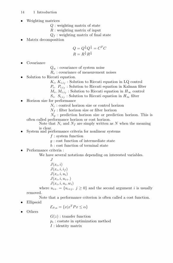
• Weighting matricesQ : weighting matrix of stateR : weighting matrix of inputQf : weighting matrix of final state

• Matrix decomposition

Q = Q12 Q

12 = CT C

R = R12 R

12

• CovarianceQw : covariance of system noiseRv : covariance of measurement noises

• Solution to Riccati equation.Ki, Ki,if

: Solution to Riccati equation in LQ controlPi, Pi,if

: Solution to Riccati equation in Kalman filterMi, Mi,if

: Solution to Riccati equation in H∞ controlSi, Si,if

: Solution to Riccati equation in H∞ filter• Horizon size for performance

Nc : control horizon size or control horizonNf : filter horizon size or filter horizonNp : prediction horizon size or prediction horizon. This is

often called performance horizon or cost horizon.Note that Nc and Nf are simply written as N when the meaningis clear.

• System and performance criteria for nonlinear systemsf : system functiong : cost function of intermediate stateh : cost function of terminal state

• Performance criteria :We have several notations depending on interested variables.

JJ(xi, i)J(xi, i, if )J(xi, i, ui)J(xi, i, ui+·)J(xi, i, ui, wi)

where ui+· = ui+j , j ≥ 0 and the second argument i is usuallyremoved.

Note that a performance criterion is often called a cost function.• Ellipsoid

EP,α = x|xT Px ≤ α• Others

G(z) : transfer functionpi : costate in optimization methodI : identity matrix

1.7 References 15

1.7 References

There are several survey papers on the existing results of predictive control[RRTP78, GPM89, RMM94, Kwo94, May95, LC97, May97, CA98, ML99,MRRS00, KHA04]. There are useful proceedings of conferences or workshopson MPC [Cla94, KGC97, AZ99, Gri02]. In [Kwo94], a very wide ranging listof references up to 1994 is provided. [AZ99, Gri02] would be helpful for thosewho are interested in nonlinear MPC. In [MRRS00], the stability and theoptimality for constrained and nonlinear predictive controls for state-spacemodels are well summarized and categorized. Recent predictive controls fornonlinear systems are surveyed in [KHA04]. In particular, comparisons amongindustrial MPCs are well presented in [QB97], [QB00], [QB03] from a practicalpoint of view.

There are several books on predictive controls [BGW90, Soe92, Mos95,MSR96, AZ00, KC00, Mac02, Ros03, HKH02, CB04]. The GPC for uncon-strained linear systems and its monotonicity conditions for guaranteeing sta-bility are given in [BGW90]. The book [Soe92] provides a comprehensive ex-position on GPC and its relationship with MPC. The book [Mos95] coverspredictive controls and adaptive predictive controls for unconstrained linearsystems with a common unifying framework. The book [AZ00] covers nonlin-ear RHC theory, computational aspects of on-line optimization and applica-tion issues. In the book [Mac02], industrial case studies are illustrated andseveral commercial predictive control products are introduced. Implementa-tion issues for predictive controls are dealt with in the book [CB04].

2

Optimal Controls on Finite and InfiniteHorizons: A Review

2.1 Introduction

In this chapter, important results on optimal controls are reviewed.Optimal controls depend on the performance criterion that should reflect

the designer’s concept of good performance. Two important performance cri-teria are considered for optimal controls. One is for minimization and theother for minimaximization.

Both nonlinear and linear optimal controls are reviewed. First, the generalresults for nonlinear systems are introduced, particularly with the dynamicprogramming and a minimum principle. Then, the optimal controls for linearsystems are obtained as a special case. Actually, linear quadratic and H∞optimal controls are introduced for both state feedback and output feedbackcontrols. Tracking controls are also introduced for future use.

Optimal controls are discussed for free and fixed terminal states. The for-mer may or may not have a terminal cost. In particular, a nonzero terminalcost for the free terminal state is called a free terminal cost in the subsequentchapters. In addition, a fixed terminal state is posed as a terminal equalityconstraint in the subsequent chapters. The optimal controls for the fixed ter-minal and nonzero reference case will be derived in this chapter. They areimportant for RHC. However, they are not common in the literature.

Linear optimal controls are transformed to SDP using LMIs for easiercomputation of the control laws. This numerical method can be useful forobtaining optimal controls in constrained systems, which will be discussedlater.

Most results given in this chapter lay the foundation for the subsequentchapters on receding horizon controls.

Proofs are generally given in order to make our presentation in this bookmore self-contained, though they appear in the existing literature. H2 filtersand H2 controls are important, but not used for subsequent chapters; thus,they are summarized without proof.

18 2 Optimal Controls on Finite and Infinite Horizons: A Review

The organization of this chapter is as follows. In Section 2.2, optimal con-trols for general systems such as dynamic programming and the minimumprinciple are dealt with for both minimum and minimax criteria. In Section2.3, linear optimal controls, such as the LQ control based on the minimumcriterion and H∞ control based on the minimax criterion, are introduced. InSection 2.4, the Kalman filter on the minimum criterion and the H∞ filteron the minimax criterion are discussed. In Section 2.5, LQG control on theminimum criterion and the output feedback H∞ control on the minimax cri-terion are introduced for output feedback optimal controls. In Section 2.6, theinfinite horizon LQ and H∞ control are represented in LMI forms. In Section2.7, H2 controls are introduced as a general approach for LQ control.

2.2 Optimal Control for General Systems

In this section, we consider optimal controls for general systems. Two ap-proaches will be taken. The first approach is based on the minimization andthe second approach is based on the minimaximization.

2.2.1 Optimal Control Based on Minimum Criterion

Consider the following discrete-time system:

xi+1 = f(xi, ui, i), xi0 = x0 (2.1)

where xi ∈ n and ui ∈ m are the state and the input respectively, and maybe required to belong to the given sets, i.e. xi ∈ X ∈ n and ui ∈ U ∈ m.

A performance criterion with the free terminal state is given by

J(xi0 , i0, u) =if−1∑i=i0

g(xi, ui, i) + h(xif, if ) (2.2)

i0 and if are the initial and terminal time. g(·, ·, ·) and h(·, ·) are specifiedscalar functions. We assume that if is fixed here for simplicity. Note thatxif

is free for the performance criterion (2.2). However, xifcan be fixed. A

performance criterion with the fixed terminal state is given by

J(xi0 , i0, u) =if−1∑i=i0

g(xi, ui, i) (2.3)

subject to

xif= xr

if(2.4)

where xrif

is given.

2.2 Optimal Control for General Systems 19

Here, the optimal control problem is to find an admissible control ui ∈ Ufor i ∈ [i0, if − 1] that minimizes the cost function (2.2) or (2.3) with theconstraint (2.4).

The Principle of Optimality and Dynamic Programming

If S-a-D is the optimal path from S to D with the cost J∗SD, then a-D is

the optimal path from a to D with J∗aD, as can be seen in Figure 2.1. This

property is called the principle of optimality. Thus, an optimal policy has theproperty that, whatever the initial state and initial decision are, the remainingdecisions must constitute an optimal policy with regard to the state resultingfrom the first decision.

SD

Fig. 2.1. Optimal path from S to D

Now, assume that there are allowable paths S-a-D, S-b-D, S-c-D, andS-d-D and optimal paths from a, b, c, and d to D are J∗

aD, J∗bD, J∗

cD, and J∗dD

respectively, as can be seen in Figure 2.2. Then, the optimal trajectory thatstarts at S is found by comparing

J∗SaD = JSa + J∗

aD

J∗SbD = JSb + J∗

bD

J∗ScD = JSc + J∗

cD

J∗SdD = JSd + J∗

dD (2.5)

The minimum of these costs must be the one associated with the optimal de-cision at point S. Dynamic programming is a computational technique whichextends the above decision-making concept to the sequences of decisions whichtogether define an optimal policy and trajectory.

Assume that the final time if is specified. If we consider the performancecriterion (2.2) subject to the system (2.1), the performance criterion of dy-namic programming can be represented by

J(xi, i, u) = g(xi, ui, i) + J∗(xi+1, i + 1), i ∈ [i0, if − 1] (2.6)J∗(xi, i) = min

uτ ,τ∈[i,if−1]J(xi, i, u)

= minui

g(xi, ui, i) + J∗(f(xi, ui, i), i + 1) (2.7)

20 2 Optimal Controls on Finite and Infinite Horizons: A Review

S D

Fig. 2.2. Paths from S through a, b, c, and d to D

where

J∗(xif, if ) = h(xif

, if ) (2.8)

For the fixed terminal state, J∗(xif, if ) = h(xif

, if ) is fixed since xifand if

are constants.It is noted that the dynamic programming method gives a closed-loop con-

trol, while the method based on the minimum principle considered next givesan open-loop control for most nonlinear systems.

Pontryagin’s Minimum Principle

We assume that the admissible controls are constrained by some boundaries,since in realistic systems control constraints do commonly occur. Physicallyrealizable controls generally have magnitude limitations. For example, thethrust of a rocket engine cannot exceed a certain value and motors provide alimited torque.

By definition, the optimal control u∗ makes the performance criterion J alocal minimum if

J(u) − J(u∗) = J ≥ 0

for all admissible controls sufficiently close to u∗. If we let u = u∗ + δu, theincrement in J can be expressed as

J(u∗, δu) = δJ(u∗, δu) + higher order terms

Hence, the necessary conditions for u∗ to be the optimal control are

δJ(u∗, δu) ≥ 0

if u∗ lies on the boundary during any portion of the time interval [i0, if ] and

δJ(u∗, δu) = 0

if u∗ lies within the boundary during the entire time interval [i0, if ].

2.2 Optimal Control for General Systems 21

We form the following augmented cost functional:

Ja =if−1∑i=i0

g(xi, ui, i) + pT

i+1[f(xi, ui, i) − xi+1]

+ h(xif, if )

by introducing the Lagrange multipliers pi0 , pi0+1, · · · , pif. For simplicity of

the notation, we denote g(x∗i , u

∗i , i) by g and f(x∗

i , u∗i , i) by f respectively.

Then, the increment of Ja is given by

Ja =if−1∑i=i0

g(x∗

i + δxi, u∗i + δui, i) + [p∗i+1 + δpi+1]T

× [f(x∗i + δxi, u

∗i + δui, i) − (x∗

i+1 + δxi+1)

+ h(x∗if

+ δxif, if )

−if−1∑i=i0

g(x∗

i , u∗i , i) + p∗T

i+1[f(x∗i , u

∗i , i) − x∗

i+1]

+ h(x∗if

, if )

=if−1∑i=i0

[∂g

∂xi

]T

δxi +[

∂g

∂ui

]T

δui + p∗Ti+1

[∂f

∂xi

]T

δxi

+ p∗Ti+1

[∂f

∂ui

]T

δui + δpTi+1f(x∗

i , u∗i , i)

− δpTi+1x

∗i+1 − p∗T

i+1δxi+1

+[

∂h

∂xif

]T

δxif

+ higher order terms (2.9)

To eliminate δxi+1, we use the fact

if−1∑i=i0

p∗Ti+1δxi+1 = p∗T

ifδxif

+if−1∑i=i0

pTi δxi

Since the initial state xi0 is given, it is apparent that δxi0 = 0 and pi0 can bechosen arbitrarily. Now, we have

Ja =if−1∑i=i0

[∂g

∂xi− p∗i +

∂f

∂xip∗i+1

]T

δxi +[

∂g

∂ui+

∂f

∂uip∗i+1

]T

δui

+δpTi+1

[f(x∗

i , u∗i , i) − x∗

i+1

]+[

∂h

∂xif

− p∗if

]T

δxif

+ higher order terms

Note that variable δxi for i = i0 + 1, · · · , if are all arbitrary. Define thefunction H, called the Hamiltonian

22 2 Optimal Controls on Finite and Infinite Horizons: A Review

H(xi, ui, pi+1, i) g(xi, ui, i) + pTi+1f(xi, ui, i)

If the state equations are satisfied, and p∗i is selected so that the coefficient ofδxi is identically zero, that is,

x∗i+1 = f(x∗

i , u∗i , i) (2.10)

p∗i =∂g

∂xi+

∂f

∂xip∗i+1 (2.11)

x∗i0 = x0 (2.12)

p∗if=

∂h

∂xif

(2.13)

then we have

Ja =if−1∑i=i0

[∂H∂u

(x∗i , u

∗i , p

∗i , i)]T

δui

+ higher order terms

The first-order approximation to the change in H caused by a change in ualone is given by[

∂H∂u

(x∗i , u

∗i , p

∗i , i)]T

δui ≈ H(x∗i , u

∗i + δui, p

∗i+1, i) −H(x∗

i , u∗i , p

∗i+1, i)

Therefore,

J(u∗, δu) =if−1∑i=i0

[H(x∗

i , u∗i + δui, p

∗i+1, i) −H(x∗

i , u∗i , p

∗i+1, i)

]+higher order terms (2.14)

If u∗ + δu is in a sufficiently small neighborhood of u∗, then the higher orderterms are small, and the summation (2.14) dominates the expression for Ja.Thus, for u∗ to be an optimal control, it is necessary that

if−1∑i=i0

[H(x∗

i , u∗i + δui, p

∗i+1, i) −H(x∗

i , u∗i , p

∗i+1, i)

]≥ 0 (2.15)

for all admissible δu. We assert that in order for (2.15) to be satisfied for alladmissible δu in the specified neighborhood, it is necessary that

H(x∗i , u

∗i + δui, p

∗i+1, i) −H(x∗

i , u∗i , p

∗i+1, i) ≥ 0 (2.16)

for all admissible δui and for all i = i0, · · · , if . In order to prove the inequality(2.15), consider the control

ui = u∗i , i /∈ [i1, i2]

ui = u∗i + δui, i ∈ [i1, i2]

(2.17)

2.2 Optimal Control for General Systems 23

where [i1, i2] is a nonzero time interval, i.e. i1 < i2 and δui is an admissiblecontrol variation that satisfies u∗ + δu ∈ U .

Suppose that inequality (2.16) is not satisfied in the interval [i1, i2] for thecontrol described in (2.17). So, we have

H(x∗i , ui, p

∗i+1, i) < H(x∗

i , u∗i , p

∗i+1, i)

in the interval [i1, i2] and the following inequality is obtained:

if−1∑i=i0

[H(x∗

i , ui, p∗i+1, i) −H(x∗

i , u∗i , p

∗i+1, i)

]

=i2∑

i=i1

[H(x∗

i , ui, p∗i+1, i) −H(x∗

i , u∗i , p

∗i+1, i)

]< 0

Since the interval [i1, i2] can be anywhere in the interval [i0, if ], it is clearthat if

H(x∗i , ui, p

∗i+1, i) < H(x∗

i , u∗i , p

∗i+1, i)

for any i ∈ [i0, if ], then it is always possible to construct an admissible control,as in (2.17), which makes Ja < 0, thus contradicting the optimality of thecontrol u∗

i . Therefore, a necessary condition for u∗i to minimize the functional

Ja isH(x∗

i , u∗i , p

∗i+1, i) ≤ H(x∗

i , ui, p∗i+1, i) (2.18)

for all i ∈ [i0, if ] and for all admissible controls. The inequality (2.18) indicatesthat an optimal control must minimize the Hamiltonian. Note that we haveestablished a necessary, but not, in general, sufficient, condition for optimality.An optimal control must satisfy the inequality (2.18). However, there may becontrols that satisfy the minimum principle that are not optimal.

We now summarize the principle results. In terms of the Hamiltonian, thenecessary conditions for u∗

i to be an optimal control are

x∗i+1 =

∂H∂pi+1

(x∗i , u

∗i , p

∗i+1, i) (2.19)

p∗i =∂H∂x

(x∗i , u

∗i , p

∗i+1, i) (2.20)

H(x∗i , u

∗i , p

∗i+1, i) ≤ H(x∗

i , ui, p∗i+1, i) (2.21)

for all admissible ui and i ∈ [i0, if − 1], and two boundary conditions

xi0 = x0, p∗if=

∂h

∂xif

(x∗if

, if )

The above result is called Pontryagin’s minimum principle. The minimumprinciple, although derived for controls in the given set U , can also be applied

24 2 Optimal Controls on Finite and Infinite Horizons: A Review

to problems in which the admissible controls are not bounded. In this case,for u∗

i to minimize the Hamiltonian it is necessary (but not sufficient) that

∂H∂ui

(x∗i , u

∗i , p

∗i+1, i) = 0, i ∈ [i0, if − 1] (2.22)

If (2.22) is satisfied and the matrix

∂2H∂u2

i

(x∗i , u

∗i , p

∗i+1, i)

is positive definite, then this is sufficient to guarantee that u∗i makes Ja a local

minimum. If the Hamiltonian can be expressed in the form

H(xi, ui, pi+1, i) = c0(xi, pi+1, i) +[c1(xi, pi+1, i)

]Tui +

12uT

i Rui

where c0(·, ·, ·) and c1(·, ·, ·) are a scalar and an m× 1 vector function respec-tively, that do not have any term containing ui, then (2.22) and ∂2H/∂u2

i > 0are necessary and sufficient for H(x∗

i , u∗i , p

∗i+1, i) to be a global minimum.

For a fixed terminal state, δxifin the last term of (2.9) is equal to zero.

Thus, (2.13) is not necessary, which is replaced with xif= xr

if.

2.2.2 Optimal Control Based on Minimax Criterion

Consider the following discrete-time system:

xi+1 = f(xi, ui, wi, i), xi0 = x0 (2.23)

with a performance criterion

J(xi0 , i0, u, w) =if−1∑i=i0

[g(xi, ui, wi, i)] + h(xif, if ) (2.24)

where xi ∈ n is the state, ui ∈ m is the input and wi ∈ l is the dis-turbance. The input and the disturbance are required to belong to the givensets, i.e. ui ∈ U and wi ∈ W. Here, the fixed terminal state is not dealt withbecause the minimax problem in this case does not make sense.

The minimax criterion we are dealing with is related to a difference game.We want to minimize the performance criterion, while disturbances try tomaximize one. A pair policies (u,w) ∈ U ×W is said to constitute a saddle-point solution if, for all (u,w) ∈ U ×W,

J(xi0 , i0, u∗, w) ≤ J(xi0 , i0, u

∗, w∗) ≤ J(xi0 , i0, u, w∗) (2.25)

We may think that u∗ is the best control, while w∗ is the worst disturbance.The existence of these u∗ and w∗ is guaranteed by specific conditions.

2.2 Optimal Control for General Systems 25

The control u∗ makes the performance criterion (2.24) a local minimum if

J(xi0 , i0, u, w) − J(xi0 , i0, u∗, w) = J ≥ 0

for all admissible controls. If we let u = u∗ + δu, the increment in J can beexpressed as

J(u∗, δu, w) = δJ(u∗, δu, w) + higher order terms

Hence, the necessary conditions for u∗ to be the optimal control are

δJ(u∗, δu, w) ≥ 0

if u∗ lies on the boundary during any portion of the time interval [i0, if ] and

δJ(u∗, δu, w) = 0

if u∗ lies within the boundary during the entire time interval [i0, if ].Meanwhile, the disturbance w∗ makes the performance criterion (2.24) a

local maximum ifJ(u,w) − J(u,w∗) = J ≤ 0

for all admissible disturbances. Taking steps similar to the case of u∗, weobtain the necessary condition

δJ(u,w∗, δw) ≤ 0

if w∗ lies on the boundary during any portion of the time interval [i0, if ] and

δJ(u,w∗, δw) = 0

if w∗ lies within the boundary during the entire time interval [i0, if ].We now summarize the principle results. In terms of the Hamiltonian, the

necessary conditions for u∗i to be an optimal control are

x∗i+1 =

∂H∂pi+1

(x∗i , u

∗i , w

∗i , p∗i+1, i)

p∗i =∂H∂xi

(x∗i , u

∗i , w

∗i , p∗i+1, i)

H(x∗i , u

∗i , wi, p

∗i+1, i) ≤ H(x∗

i , u∗i , w

∗i , p∗i+1, i) ≤ H(x∗

i , ui, w∗i , p∗i+1, i)

for all admissible ui and wi on the i ∈ [i0, if −1], and two boundary conditions

xi0 = x0, p∗if=

∂h

∂xif

(x∗if

, if )

Now, a dynamic programming for minimaxization criterion is explained.Let there exist a function J∗(xi, i), i ∈ [i0, if − 1] such that

26 2 Optimal Controls on Finite and Infinite Horizons: A Review

J∗(xi, i) = minu∈U

maxw∈W

[g(xi, ui, wi, i) + J∗(f(xi, ui, wi, i), i + 1)

]= max

w∈Wminu∈U

[g(xi, ui, wi, i) + J∗(f(xi, ui, wi, i), i + 1)

]J∗(xif

, if ) = h(xif, if ) (2.26)

Then a pair of u and w that is generated by (2.26) provides a saddle pointwith the corresponding value given by J∗(xi0 , i0).

2.3 Linear Optimal Control with State Feedback

2.3.1 Linear Quadratic Controls Based on Minimum Criterion

In this section, an LQ control in a tracking form for discrete time-invariantsystems is introduced in a state-feedback form. We consider the followingdiscrete time-invariant system:

xi+1 = Axi + Bui

zi = Czxi (2.27)

There are two methods which are used to obtain the control of minimizingthe chosen cost function. One is dynamic programming and the other is theminimum principle of Pontryagin. The minimum principle of Pontryagin anddynamic programming were briefly introduced in the previous section. In themethod of dynamic programming, an optimal control is obtained by employingthe intuitively appealing concept called the principle of optimality. Here, weuse the minimum principle of Pontryagin in order to obtain an optimal finitehorizon LQ tracking control (LQTC).

We can divide the terminal states into two cases. The first case is a freeterminal state and the second case is a fixed terminal state. In the following,we will derive two kinds of LQ controls in a tracking form.

1 ) Free Terminal State

The following quadratic performance criterion is considered:

J(zr, u·) =if−1∑i=i0

[(zi − zri )T Q(zi − zr

i ) + uTi Rui]

+ [zif− zr

if]T Qf [zif

− zrif

] (2.28)

Here, xi ∈ n, ui ∈ m, zi ∈ p, zri , Q > 0, R > 0, Qf > 0 are the state,

the input, the controlled output, the command signal or the reference signal,the state weighting matrix, the input weighting matrix, and the terminal

2.3 Linear Optimal Control with State Feedback 27

weighting matrix respectively. Here, zri0

, zri0+1, · · · , zr

ifare command signals

which are assumed to be available over the future horizon [i0, if ].For tracking problems, with Q > 0 and Qf > 0 in (2.28), there is a

tendency that zi → zri . In order to derive the optimal tracking control which

minimizes the performance criterion (2.28), it is convenient to express theperformance criterion (2.28) with the state xi instead of zi. It is well knownthat for a given p × n (p ≤ n) full rank matrix Cz there always exist somen × p matrices L such that CzL = Ip×p. Let

xri = Lzr

i (2.29)

The performance criterion (2.28) is then rewritten as

J(xr, u) =if−1∑i=i0

[(xi − xri )

T CTz QCz(xi − xr

i ) + uTi Rui]

+ [xif− xr

if]T CT

z QfCz[xif− xr

if] (2.30)

The performance criterion (2.30) can be written as

J(xr, u) =if−1∑i=i0

[(xi − xr

i )T Q(xi − xr

i ) + uTi Rui

]+ (xif

− xrif

)T Qf (xif− xr

if) (2.31)

where

Q = CTz QCz and Qf = CT

z QfCz (2.32)

Q and Qf in (2.31) can be independent design parameters ignoring the relation(2.32). That is, the matrices Q and Qf can be positive definite, if necessary,though Q and Qf in (2.32) are semidefinite when Cz is not of full rank. Inthis book, Q and Qf in (2.31) are independent design parameters. However,whenever necessary, we will make some connections to (2.32).

We first form a Hamiltonian:

Hi = [(xi − xri )

T Q(xi − xri ) + uT

i Rui] + pTi+1[Axi + Bui] (2.33)

where i ∈ [i0, if − 1]. According to (2.20) and (2.2.1), we have

pi =∂Hi

∂xi= 2Q(xi − xr

i ) + AT pi+1 (2.34)

pif=

∂h(xif, if )

∂xif

= 2Qf (xif− xr

if) (2.35)

where h(xif, if ) = (xif

− xrif

)T Qf (xif− xr

if).

28 2 Optimal Controls on Finite and Infinite Horizons: A Review

A necessary condition for ui to minimize Hi is ∂Hi

∂ui= 0. Thus, we have

∂Hi

∂ui= 2Rui + BT pi+1 = 0 (2.36)

Since the matrix ∂2Hi

∂u2i

= 2R is positive definite and Hi is a quadratic formin u, the solution of (2.36) is an optimal control to minimize Hi. The optimalsolution u∗

i is

u∗i = −1

2R−1BT pi+1 (2.37)

If we assume that

pi = 2Ki,ifxi + 2gi,if

(2.38)

the solution to the optimal control problem can be reduced to finding thematrices Ki,if

and gi,if. From (2.35), the boundary conditions are given by

Kif ,if= Qf (2.39)

gif ,if= −Qfxr

if(2.40)

Substituting (2.27) into (2.38) and replacing ui with (2.37), we have

pi+1 = 2Ki+1,ifxi+1 + 2gi+1,if

= 2Ki+1,if(Axi + Bui) + 2gi+1,if

= 2Ki+1,if(Axi −

12BR−1BT pi+1) + 2gi+1,if

(2.41)

Solving for pi+1 in (2.41) yields the following equation:

pi+1 = [I + Ki+1,ifBR−1BT ]−1[2Ki+1,if

Axi + 2gi+1,if] (2.42)

Substituting for pi+1 from (2.37), we can write

u∗i = −R−1BT [I + Ki+1,if

BR−1BT ]−1[Ki+1,ifAxi + gi+1,if

] (2.43)

What remains to do is to find Ki,ifand gi,if

. If we put the equation (2.42)into the equation (2.34), we have

pi = 2Q(xi − xri ) + AT [I + Ki+1,if

BR−1BT ]−1[2Ki+1,ifAxi + 2gi+1,if

],

= 2[Q + AT (I + Ki+1,ifBR−1BT )−1Ki+1,if

A]xi

+2[−Qxri + AT (I + Ki+1,if

BR−1BT )−1gi+1,if] (2.44)

The assumption (2.38) holds by choosing Ki,ifand gi,if

as

2.3 Linear Optimal Control with State Feedback 29

Ki,if= AT [I + Ki+1,if

BR−1BT ]−1Ki+1,ifA + Q

= AT Ki+1,ifA − AT Ki+1,if

B(R + BT Ki+1,ifB)−1BT Ki+1,if

A

+ Q (2.45)gi,if

= AT [I + Ki+1,ifBR−1BT ]−1gi+1,if

− Qxri (2.46)

where the second equality comes from

[I + Ki+1,ifBR−1BT ]−1 = I − Ki+1,if

B(R + BT Ki+1,ifB)−1BT (2.47)

using the matrix inversion lemma (A.2) in Appendix A. The optimal controlderived until now is summarized in the following theorem.

Theorem 2.1. In the system (2.27), the LQTC for the free terminal state isgiven as (2.43) for the performance criterion (2.31). Ki,if

and gi,ifin (2.43)

are obtained from Riccati Equation (2.45) and (2.46) with boundary condition(2.39) and (2.40).

Depending on Qf , Ki,ifmay be nonsingular (positive definite) or singular

(positive semidefinite). This property will be important for stability and theinversion of the matrix Ki,if

in coming sections.For a zero reference signal, gi,if

becomes zero so that we have

u∗i = −R−1BT [I + Ki+1,if

BR−1BT ]−1Ki+1,ifAxi (2.48)

The performance criterion (2.31) associated with the optimal control (2.43) isgiven in the following theorem.

Theorem 2.2. The optimal cost J∗(xi) with the reference value can be given

J∗(xi) = xTi Ki,if

xi + 2xTi gi,if

+ wi,if(2.49)

where

wi,if= wi+1,if

+ xrTi Qxr

i − gTi+1,if

B(BT Ki+1,ifB + R)−1BT gi+1,if

(2.50)

with boundary condition wif ,if= xrT

ifQfxr

if.

Proof. A long and tedious calculation is required to obtain the optimal cost us-ing the result of Theorem 2.1. Thus, we derive the optimal cost using dynamicprogramming, where the optimal control and the optimal cost are obtainedsimultaneously.

Let J∗(xi+1) denote the optimal cost associated with the initial state xi+1

and the interval [i + 1, if ]. Suppose that the optimal cost J∗(xi+1) is given as

J∗(xi+1) = xTi+1Ki+1,if

xi+1 + 2xTi+1gi+1,if

+ wi+1,if(2.51)

where wi+1,ifwill be determined later. We wish to calculate the optimal cost

J∗(xi) from (2.51).

30 2 Optimal Controls on Finite and Infinite Horizons: A Review

By applying the principle of optimality, J∗(xi) can be represented as fol-lows:

J∗(xi) = minui

[(xi − xr

i )T Q(xi − xr

i ) + uTi Rui + J∗(xi+1)

](2.52)

(2.52) can be evaluated backward by starting with the condition J∗(xif) =

(xif− xr

if)T Qf (xif

− xrif

).Substituting (2.27) and (2.51) into (2.52), we have

J∗(xi) = minui

[(xi − xr

i )T Q(xi − xr

i ) + uTi Rui + xT

i+1Ki+1,ifxi+1

+ 2xTi+1gi+1,if

+ wi+1,if

](2.53)

= minui

[(xi − xr

i )T Q(xi − xr

i ) + uTi Rui

+ (Axi + Bui)T Ki+1,if(Axi + Bui) + 2(Axi + Bui)T gi+1,if

+ wi+1,if

](2.54)

Note that J∗(xi) has a quadratic equation with respect to ui and xi. For agiven xi, the control ui is chosen to be optimal according to (2.54). Takingderivatives of (2.54) with respect to ui to obtain

∂J∗(xi)∂ui

= 2Rui + 2BT Ki+1,ifBui + 2BT Ki+1,if

Axi + 2BT gi+1,if= 0

we have the following optimal control ui:

ui = −(R + BT Ki+1,ifB)−1[BT Ki+1,if

Axi + BT gi+1,if] (2.55)

= −L1,ixi + L2,igi+1,if(2.56)

where

L1,i= [R + BT Ki+1,if

B]−1BT Ki+1,ifA (2.57)

L2,i= −[R + BT Ki+1,if

B]−1BT (2.58)

It is noted that the optimal control ui in (2.56) is the same as (2.43) derivedfrom the minimum principle. How to obtain the recursive equations of Ki+1,if

and gi+1,ifis discussed later.

From definitions (2.57) and (2.58), we have the following relations:

AT Ki+1,ifB[R + BT Ki+1,if

B]−1BT Ki+1,ifA = AT Ki+1,if

BL1,i

= LT1,iB

T Ki+1,ifA

= LT1,i[R + BT Ki+1,if

B]L1,i

(2.59)

2.3 Linear Optimal Control with State Feedback 31

where the most left side is equivalent to the second term of Riccati Equation(2.45) and these relations are useful for representing the Riccati equation interms of closed-loop system A − BL1,i.

Substituting (2.56) into (2.54) yields

J∗(xi) = xTi

[Q + LT

1,iRL1,i + (A − BL1,i)T Ki+1,if(A − BL1,i)

]xi

+ 2xTi

[−LT

1,iRL2,igi+1,if+ (A − BL1,i)T Ki+1,if

BL2,igi+1,if

+ (A − BL1,i)T gi+1,if− Qxr

i

]+gT

i+1,ifLT

2,iRL2,igi+1,if

+ gTi+1,if

LT2,iB

T Ki+1,ifBL2,igi+1,if

+ 2gTi+1,if

LT2,iB

T gi+1,if+ wi+1,if

+ xrTi Qxr

i (2.60)

where the terms are arranged according to the order of xi. The quadraticterms with respect to xi in (2.60) can be reduced to xT

i Ki,ifxi from Riccati

Equation given by

Ki,if= [A − BL1,i]T Ki+1,if

[A − BL1,i] + LT1,iRL1,i + Q (2.61)

which is the same as (2.45) according to the relation (2.59).The first-order coefficients with respect to xi in (2.60) can be written as

− LT1,iRL2,igi+1,if

+ (A − BL1,i)T Ki+1,ifBL2,igi+1,if

+ (A − BL1,i)T gi+1,if− Qxr

i

= −LT1,iRL2,igi+1,if

+ AT Ki+1,ifBL2,igi+1,if

− LT1,iB

T Ki+1,ifBL2,igi+1,if

+ AT gi+1,if− LT

1,iBT gi+1,if

− Qxri

= −AT [KTi+1,if

B(R + BT Ki+1,ifB)−1BT − I]gi+1,if

− Qxri

= AT [I + KTi+1,if

BR−1B]−1gi+1,if− Qxr

i

which can be reduced to gi,ifif it is generated from (2.46).

The terms without xi in (2.60) can be written as

gTi+1,if

LT2,iRL2,igi+1,if

+ gTi+1,if

LT2,iB

T Ki+1,ifBL2,igi+1,if

+ 2gTi+1,if

LT2,iB

T gi+1,if+ wi+1,if

+ xrTi Qxr

i

= gTi+1,if

B[R + BT Ki+1,ifB]−1BT gi+1,if

− 2gTi+1,if

B[R + BT Ki+1,ifB]−1BT gi+1,if

+ wi+1,if+ xrT

i Qxri

= −gTi+1,if

B[R + BT Ki+1,ifB]−1BT gi+1,if

+ wi+1,if+ xrT

i Qxri

which can be reduced to wi,ifif it is defined as (2.50). If gi,if

and wi,ifare

chosen as (2.46) and (2.50), then J∗(xi) is in a form such as (2.51), i.e.

32 2 Optimal Controls on Finite and Infinite Horizons: A Review

J∗(xi) = xTi Ki,if

xi + 2xTi gi,if

+ wi,if(2.62)

Now, we have only to find the boundary value of gi,ifand wi,if

. J∗(xif) should

be equal to the performance criterion for the final state. Thus, wif ,ifand gif ,if

should be chosen as wif ,if= xrT

ifQfxr

ifand gif ,if

= −Qfxrif

so that we have

J∗(xif) = xT

ifKif ,if

xif+ 2xT

ifgif ,if

+ wif ,if

= xTif

Qfxif− 2xT

ifQfxr

if+ xrT

ifQfxr

if

= (xif− xr

if)T Qf (xif

− xrif

)

This completes the proof.

The result of Theorem 2.2 will be utilized only for zero reference signalsin subsequent sections.

For positive definite Qf and nonsingular matrix A, we can have anotherform of the above control (2.43). Let Pi,if

= K−1i,if

if the inverse of Ki,ifexists.

Then (2.45) can be represented by

P−1i,if

= AT [I + P−1i+1,if

BR−1BT ]−1P−1i+1,if

A + Q (2.63)

Pi,if=

AT [Pi+1,if+ BR−1BT ]−1A + Q

−1

(2.64)

Let Pi,if= Pi,if

+ BR−1BT . Then

Pi,if= (AT P−1

i+1,ifA + Q)−1 + BR−1BT

= A−1(P−1i+1,if

+ A−T QA−1)−1A−T + BR−1BT

= A−1[I + Pi+1,ifA−T QA−1]−1Pi+1,if

A + BR−1BT (2.65)

gi,if= AT [I + P−1

i+1,ifBR−1BT ]−1gi+1,if

− Qxri

= AT [Pi+1,if+ BR−1BT ]−1Pi+1,if

gi+1,if− Qxr

i

= AT P−1i+1,if

(Pi+1,if− BR−1BT )gi+1,if

− Qxri (2.66)

with the boundary condition

Pif ,if= Q−1

f + BR−1BT (2.67)

Using the following relation:

−[I + R−1BT P−1i+1,if

B]−1R−1BT P−1i+1,if

Axi

= −R−1BT P−1i+1,if

[I + BR−1BT P−1i+1,if

]−1Axi

= −R−1BT [Pi+1,if+ BR−1BT ]−1Axi

= −R−1BT P−1i+1,if

Axi

2.3 Linear Optimal Control with State Feedback 33

and

−[I + R−1BT P−1i+1,if

B]−1R−1Bgi+1,if

= R−1B[I + P−1i+1,if

BR−1BT ]−1gi+1,if

= R−1BP−1i+1,if

(Pi+1,if− BR−1BT )gi+1,if

we can represent the control in another form:

u∗i = −R−1BT P−1

i+1,if[Axi + (Pi+1,if

− BR−1BT )gi+1,if] (2.68)

where Pi+1,ifand gi+1,if

are obtained from (2.65) and (2.66) with boundaryconditions (2.67) and (2.40) respectively.

2 ) Fixed Terminal State

Here, the following performance criterion is considered:

J(xr, u) =if−1∑i=i0

[(xi − xr

i )T Q(xi − xr

i ) + uTi Rui

](2.69)

xif= xr

if(2.70)

For easy understanding, we start off from a simple case.

Case 1: zero state weighting

Now, our terminal objective will be to make xifmatch exactly the desired

final reference state xrif

. Since we are demanding that xifbe equal to a known

desired xrif

, the final state has no effect on the performance criterion (2.31). Itis therefore redundant to include a final state weighting term in a performancecriterion. Accordingly, we may as well set Qf = 0.

Before we go to the general problem, we first consider a simple case forthe following performance criterion:

Ji0 =12

if−1∑i=i0

uTi Rui (2.71)

where Q = 0. Observe that the weighting matrix for the state becomes zero.As mentioned before, we require the control to drive xi0 exactly to

xif= xr

if(2.72)

using minimum control energy. The terminal condition can be expressed by

xif= Aif−i0xi0 +

if−1∑i=i0

Aif−i−1Bui = xrif

(2.73)

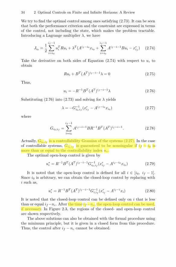
34 2 Optimal Controls on Finite and Infinite Horizons: A Review

We try to find the optimal control among ones satisfying (2.73). It can be seenthat both the performance criterion and the constraint are expressed in termsof the control, not including the state, which makes the problem tractable.Introducing a Lagrange multiplier λ, we have

Ji0 =12

if−1∑i=i0

uTi Rui + λT (Aif−i0xi0 +

if−1∑i=i0

Aif−i−1Bui − xrif

) (2.74)

Take the derivative on both sides of Equation (2.74) with respect to ui toobtain

Rui + BT (AT )if−i−1λ = 0 (2.75)

Thus,

ui = −R−1BT (AT )if−i−1λ (2.76)

Substituting (2.76) into (2.73) and solving for λ yields

λ = −G−1i0,if

(xrif

− Aif−i0xi0) (2.77)

where

Gi0,if=

if−1∑i=i0

Aif−i−1BR−1BT (AT )if−i−1. (2.78)

Actually, Gi0,ifis a controllability Gramian of the systems (2.27). In the case

of controllable systems, Gi0,ifis guaranteed to be nonsingular if if − i0 is

more than or equal to the controllability index nc.The optimal open-loop control is given by

u∗i = R−1BT (AT )if−i−1G−1

i0,if(xr

if− Aif−i0xi0) (2.79)

It is noted that the open-loop control is defined for all i ∈ [i0, if − 1].Since i0 is arbitrary, we can obtain the closed-loop control by replacing withi such as,

u∗i = R−1BT (AT )if−i−1G−1

i,if(xr

if− Aif−ixi) (2.80)

It is noted that the closed-loop control can be defined only on i that is lessthan or equal if −nc. After the time if −nc, the open-loop control can be used,if necessary. In Figure 2.3, the regions of the closed- and open-loop controlare shown respectively.

The above solutions can also be obtained with the formal procedure usingthe minimum principle, but it is given in a closed form from this procedure.Thus, the control after if − nc cannot be obtained.

2.3 Linear Optimal Control with State Feedback 35

Fig. 2.3. Region of the closed-loop solution

Case 2: nonzero state weighting

We derive the optimal solution for the fixed terminal state from that for thefree terminal state by setting Qf = ∞I. We assume that A is nonsingular.

Since Kif ,if= Qf = ∞I, the boundary condition of Pi,if

becomes

Pif ,if= BR−1BT (2.81)

from (2.67). From (2.65), we know that Equation (2.81) is satisfied with an-other terminal condition:

Pif+1,if +1 = 0 (2.82)

It is noted that Pi+1,ifcan be singular on [if − nc + 2, if ]. Therefore, gi,if

cannot be generated from (2.66) and the control (2.68) does not make sense.However, the control for the zero reference signal can be represented as

u∗i = −R−1BT P−1

i+1,ifAxi (2.83)

where gi,ifis not necessary.

For nonzero reference signals we will take an approach called the sweepmethod. The state and costate equations are the same as those of the freeterminal case:

ui = −R−1BT pi+1 (2.84)xi+1 = Axi − BR−1BT pi+1 (2.85)

pi = Q(xi − xri ) + AT pi+1 (2.86)

36 2 Optimal Controls on Finite and Infinite Horizons: A Review

We try to find an optimal control to ensure xif= xr

if. Assume the following

relation:

pi = Kixi + Mipif+ gi (2.87)

where we need to find Si, Mi, and gi satisfying the boundary conditions

Kif= 0

Mif= I

gif= 0

respectively. Combining (2.85) with (2.87) yields the following optimal trajec-tory:

xi+1 = (I + BR−1BT Ki+1)−1(Axi − BR−1BT Mi+1pif

− BR−1BT gi+1) (2.88)

Substituting (2.87) into (2.86) provides

Kixi + Mipif+ gi = Q(xi − xr

i ) + AT [Ki+1xi+1 + Mi+1pif+ gi+1] (2.89)

Substituting xi+1 in (2.88) into (2.89) yields

[−Ki + AT Ki+1(I + BR−1BT Ki+1)−1A + Q]xi +[−Mi − AT Ki+1(I + BR−1BT Ki+1)−1BR−1BT Mi+1 + AT Mi+1]pif

+

[−gi + AT gi+1 − AT Ki+1(I + BR−1BT Ki+1)−1BR−1BT gi+1 − Qxri ] = 0

Since this equality holds for all trajectories xi arising from any initial conditionxi0 , each term in brackets must vanish. The matrix inversion lemma, therefore,yields the Riccati equation

Ki = AT Ki+1(I + BR−1BT Ki+1)−1A + Q (2.90)

and the auxiliary homogeneous difference equation

Mi = AT Mi+1 − AT Ki+1(I + BR−1BT Ki+1)−1BR−1BT Mi+1

gi = AT gi+1 − AT Ki+1(I + BR−1BT Ki+1)−1BR−1BT gi+1 − Qxri

We assume that xrif

is a linear combination of xi, pif, and some specific matrix

Ni for all i, i.e.

xrif

= Uixi + Sipif+ hi (2.91)

Evaluating for i = if yields

Uif= I (2.92)

Sif= 0 (2.93)

hif= 0 (2.94)

2.3 Linear Optimal Control with State Feedback 37

Clearly, then

Ui = MTi (2.95)

The left-hand side of (2.91) is a constant, so take the difference to obtain

0 = Ui+1xi+1 + Si+1pif+ hi+1 − Uixi − Sipif

− hi (2.96)

Substituting xi+1 in (2.88) into (2.96) and rearranging terms, we have

[Ui+1A − B(BT Ki+1B + R)−1BT Ki+1A − Ui]xi

+ [Si+1 − Si − Ui+1B(BT Ki+1B + R)−1BT Mi+1]pif

+ hi+1 − hi − Ui+1(I + BR−1BT Ki+1)−1BR−1BT gi+1 = 0 (2.97)

The first term says that

Ui = Ui+1A − B(BT Ki+1B + R)−1BT Ki+1A (2.98)

The second and third terms now yield the following recursive equations:

Si = Si+1 − MTi+1B(BT Ki+1B + R)−1BT Mi+1 (2.99)

hi = hi+1 − MTi+1(I + BR−1BT Ki+1)−1BR−1BT gi+1 (2.100)

We are now in a position to determine pif. From (2.91), we have

pif= S−1

i0(xr

if− MT

i0xi0 − hi0) (2.101)

We can now finally compute the optimal control

ui = −R−1BT [Ki+1xi+1 + Mi+1pif+ gi+1] (2.102)

by substituting (2.87) into (2.84).ui can be represented in terms of the current state xi:

ui = −R−1BT (I + Ki+1BR−1BT )−1[Ki+1Axi + Mi+1pif+ gi+1],

= −R−1BT (I + Ki+1BR−1BT )−1[Ki+1Axi + Mi+1S−1i0

(xrif

− MTi0xi0 − hi0) + gi+1] (2.103)

What we have done so far is summarized in the following theorem.

Theorem 2.3. The LQTC for the fixed terminal state is given in (2.103). Si,Mi, Pi, gi, hi are as follows:

Ki = AT Ki+1(I + BR−1BT Ki+1)−1A + Q

Mi = AT Mi+1 − AT Ki+1(I + BR−1BT Ki+1)−1BR−1BT Mi+1

Si = Si+1 − MTi+1B(BT Ki+1B + R)−1BT Mi+1

gi = AT gi+1 − AT Ki+1(I + BR−1BT Ki+1)−1BR−1BT gi+1 − Qxri

hi = hi+1 − MTi+1(I + BR−1BT Ki+1)−1BR−1BT gi+1

38 2 Optimal Controls on Finite and Infinite Horizons: A Review

where

Kif= 0, Mif

= I, Sif= 0, gif

= 0, hif= 0

It is noted that the control (2.103) is a state feedback control with respectto the current state and an open-loop control with respect to the initial state,which looks somewhat awkward at first glance. However, if the receding hori-zon scheme is adopted, then we can obtain the state feedback control thatrequires only the current state, not other past states. That will be covered inthe next chapter.

Replacing i0 with i in (2.103) yields the following closed-loop control:

ui = −R−1BT (I + Ki+1BR−1BT )−1[Ki+1Axi + Mi+1S−1i

× (xrif

− MTi xi − hi) + gi+1] (2.104)

where Si is guaranteed to be nonsingular on i ≤ if − nc.If Q in (2.103) becomes zero, then (2.103) is reduced to (2.79), which is

left as a problem at the end of this chapter.For the zero reference signal, gi and hi in Theorem 2.3 become zero due

to xri = 0. Thus, we have

ui = −R−1BT (I + Ki+1BR−1BT )−1[Ki+1A − Mi+1S−1i MT

i ]xi (2.105)

in the form of the closed-loop control. As seen above, it is a little complexto obtain the closed-form solution for the fixed terminal state problem withnonzero reference signals.

Example 2.1

The LQTC (2.103) with the fixed terminal state is a new type of a track-ing control. It is demonstrated through a numerical example.

Consider the following state space model:

xk+1 =

⎡⎣0.013 0.811 0.1230.004 0.770 0.0960.987 0.903 0.551

⎤⎦xk +

⎡⎣0.4560.0180.821

⎤⎦uk (2.106)

Q and R in the performance criterion (2.69) are set to 100I and I respectively.The reference signal and state trajectories can be seen in Figure 2.4 where thefixed terminal condition is met. A batch form solution for the fixed terminalstate is given in Section 3.5, and its computation turns out to be the same asthat of (2.103).

2.3 Linear Optimal Control with State Feedback 39

0 10 20 30 40 50 60 700

0.5

1

1.5

2

2.5

3

Reference

Recursive

Batch

(a) First component of the state

0 10 20 30 40 50 60 700

0.5

1

1.5

2

2.5

Reference

Recursive Batch

(b) Second component of the state

0 10 20 30 40 50 60 700

1

2

3

4

5

6

7

Reference

Recursive Batch

(c) Third component of the state

Fig. 2.4. State trajectory of Example 2.1

40 2 Optimal Controls on Finite and Infinite Horizons: A Review

Infinite Horizon Case

If if goes to ∞ in (2.43), (2.45), and (2.46), an infinite horizon LQTC isgiven by

u∗i = −[I + R−1BT K∞B]−1R−1BT [K∞Axi + gi+1,∞]

= −[R + BT K∞B]−1BT [K∞Axi + g∞] (2.107)

where K∞ is a solution of the following algebraic Riccati Equation (ARE):

K∞ = AT [I + K∞BR−1BT ]−1K∞A + Q (2.108)= AT K∞A − AT K∞B[R + BK∞BT ]−1BT K∞A + Q (2.109)

and g∞ is given by

g∞ = AT [I + K∞BR−1BT ]−1g∞ − Qxr (2.110)

with a fixed reference signal xr. The stability and an existence of the solutionto the Riccati equation are summarized as follows:

Theorem 2.4. If (A,B) is controllable and (A,Q12 ) is observable, the solution

to Riccati Equation (2.108) is unique and positive definite, and the stabilityof ui (2.107) is guaranteed.

We can see a proof of Theorem 2.4 in much of the literature, e.g. in[Lew86a]. The conditions on controllability and observability in Theorem 2.4can be weakened to the reachability and detectability.

Here, we shall present the return difference equality for the infinite horizonLQ control and introduce some robustness in terms of gain and phase margins.From the following simple relation:

K∞ − AT K∞A = (z−1I − A)T K∞(zI − A) + (z−1I − A)T K∞A

+ AT K∞(zI − A) (2.111)

K∞−AT K∞A in (2.111) is replaced with −AT K∞B(BT K∞B+R)−1BT K∞A−Q according to (2.109) to give

(z−1I − A)T K∞(zI − A) + (z−1I − A)T K∞A + AT K∞(zI − A)+AT K∞B(BT K∞B + R)−1BT K∞A = Q (2.112)

Pre- and post-multiply (2.112) by BT (z−1I − A)−T and (zI − A)−1Brespectively to get

BT K∞B + BT K∞A(zI − A)−1B + BT (z−1I − A)−T AT K∞B

+ BT (z−1I − A)−T AT K∞B(BT K∞B + R)−1BT K∞A(zI − A)−1B

= BT (z−1I − A)−T Q(zI − A)−1B (2.113)

2.3 Linear Optimal Control with State Feedback 41

Adding R to both sides of (2.113) and factorizing it yields the following equa-tion:

BT (z−1I − A)−T Q(zI − A)−1B + R

= [I + K∞(z−1I − A)−1B]T (BT K∞B + R)[I + K∞(zI − A)−1B] (2.114)

where K∞ = [R + BT K∞B]−1BT K∞A.From Equation (2.114), we are in a position to check gain and phase mar-

gins for the infinite horizon LQ control. First, let F (z) be I +K∞(zI−A)−1B,which is called a return difference matrix. It follows from (2.114) that

BT K∞B + R = F−T (z−1)[R + BT (z−1I − A)−T Q(zI − A)−1B]F−1(z)

which implies that

σ(BT K∞B + R) ≥ σ2(F−1(z))× σ[R + BT (z−1I − A)−T Q(zI − A)−1B] (2.115)

Note that σ(MT SM) ≥ σ(S)σ2(M) for S ≥ 0. Recalling the two factsσ[F−1(z)] = σ−1[F (z)] and σ(I − z−1A) ≤ 1 + σ(A) for |z| = 1, we have

σ[R + BT (z−1I − A)−T Q(zI − A)−1B]

≥ σ(R)σ[I + R− 12 BT (z−1I − A)−T Q(zI − A)−1BR− 1

2 ]≥ σ(R)[1 + σ−1(R)σ2(B)σ(Q)σ−2(I − z−1A)α]

≥ σ(R)σ(R)

[σ(R) + σ2(B)σ(Q)1 + σ(A)−2α] (2.116)

where α is 1 when p ≤ q and 0 otherwise. Recall that the dimensions of inputsui and outputs yi are p and q respectively. Substituting (2.116) into (2.115)and arranging terms yields

σ2[F (z)] ≥ σ(R)/σ(R)σ(R) + σ2(B)σ(K∞)

[σ(R) + σ2(B)σ(Q)1 + σ(A)−2α]

= R2

f (2.117)

Let a circle of radius Rf centered at (−1, 0) be C(−1, Rf ). The Nyquistplot of the open-loop system of the optimal regulator lies outside C(−1, Rf )for an SISO system, as can be seen in Figure 2.5; the guaranteed gain marginsGM of a control are given by

(1 + Rf )−1 ≤ GM ≤ (1 − Rf )−1 (2.118)

and the phase margins PM of the control are given by

−2 sin−1(Rf

2) ≤ PM ≤ 2 sin−1(

Rf

2) (2.119)

It is noted that margins for discrete systems are smaller than those forcontinuous systems, i.e. 0.5 ≤ GM < ∞, and −π/3 ≤ PM ≤ π/3.

42 2 Optimal Controls on Finite and Infinite Horizons: A Review

Fig. 2.5. Nyquist plot

2.3.2 H∞ Control Based on Minimax Criterion

In this subsection we derive an H∞ tracking control (HTC) for discrete time-invariant systems in a state-feedback form. Consider the following discretetime-invariant system:

xi+1 = Axi + Bwwi + Bui

zi =[

Q12 xi

R12 ui

](2.120)

where xi ∈ n denotes the state, wi ∈ l the disturbance, ui ∈ m the controlinput, and zi ∈ q+n the controlled variable which needs to be regulated. TheH∞ norm of Tzw(ejw) can be represented as

‖Tzw(ejw)‖∞ = supwi

σ(Tzw(ejw)) = supwi

∑∞i=i0

[xTi Qxi + uT

i Rui]∑∞i=i0

wTi wi

= sup‖wi‖2=1

∞∑i=i0

[xTi Qxi + uT

i Rui] = γ∗2 (2.121)

where Tzw(ejw) is a transfer function from wi to zi and σ(·) is the maximumsingular value. zi in (2.120) is chosen to make a quadratic cost function as(2.121).

The H∞ norm of the systems is equal to the induced L2 norm. The H∞control is obtained so that the H∞ norm is minimized with respect to ui.

However, it is hard to achieve an optimal H∞ control. Instead of theabove performance criterion, we can introduce a suboptimal control such that

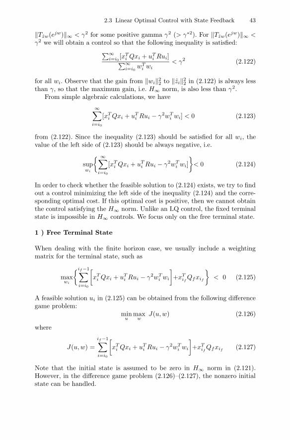
2.3 Linear Optimal Control with State Feedback 43

‖Tzw(ejw)‖∞ < γ2 for some positive gamma γ2 (> γ∗2). For ‖Tzw(ejw)‖∞ <γ2 we will obtain a control so that the following inequality is satisfied:∑∞

i=i0[xT

i Qxi + uTi Rui]∑∞

i=i0wT

i wi< γ2 (2.122)

for all wi. Observe that the gain from ‖wi‖22 to ‖zi‖2

2 in (2.122) is always lessthan γ, so that the maximum gain, i.e. H∞ norm, is also less than γ2.

From simple algebraic calculations, we have

∞∑i=i0

[xTi Qxi + uT

i Rui − γ2wTi wi] < 0 (2.123)

from (2.122). Since the inequality (2.123) should be satisfied for all wi, thevalue of the left side of (2.123) should be always negative, i.e.

supwi

∞∑i=i0

[xTi Qxi + uT

i Rui − γ2wTi wi]

< 0 (2.124)

In order to check whether the feasible solution to (2.124) exists, we try to findout a control minimizing the left side of the inequality (2.124) and the corre-sponding optimal cost. If this optimal cost is positive, then we cannot obtainthe control satisfying the H∞ norm. Unlike an LQ control, the fixed terminalstate is impossible in H∞ controls. We focus only on the free terminal state.

1 ) Free Terminal State

When dealing with the finite horizon case, we usually include a weightingmatrix for the terminal state, such as

maxwi

if−1∑i=i0

[xT

i Qxi + uTi Rui − γ2wT

i wi

]+xT

ifQfxif

< 0 (2.125)

A feasible solution ui in (2.125) can be obtained from the following differencegame problem:

minu

maxw

J(u,w) (2.126)

where

J(u,w) =if−1∑i=i0

[xT

i Qxi + uTi Rui − γ2wT

i wi

]+xT

ifQfxif

(2.127)

Note that the initial state is assumed to be zero in H∞ norm in (2.121).However, in the difference game problem (2.126)–(2.127), the nonzero initialstate can be handled.

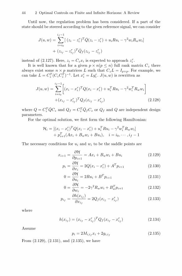
44 2 Optimal Controls on Finite and Infinite Horizons: A Review

Until now, the regulation problem has been considered. If a part of thestate should be steered according to the given reference signal, we can consider

J(u,w) =if−1∑i=i0

[ (zi − zri )T Q(zi − zr

i ) + uiRui − γ2wiRwwi]

+ (zif− zr

if)T Qf (zif

− zrif

)

instead of (2.127). Here, zi = Czxi is expected to approach zri .

It is well known that for a given p × n(p ≤ n) full rank matrix Cz therealways exist some n × p matrices L such that CzL = Ip×p. For example, wecan take L = CT

z (CzCTz )−1. Let xr

i = Lyri . J(u,w) is rewritten as

J(u,w) =if−1∑i=i0

[(xi − xr

i )T Q(xi − xr

i ) + uTi Rui − γ2wT

i Rwwi

]+(xif

− xrif

)T Qf (xif− xr

if) (2.128)

where Q = CTz QCz and Qf = CT

z QfCz or Qf and Q are independent designparameters.

For the optimal solution, we first form the following Hamiltonian:

Hi = [(xi − xri )

T Q(xi − xri ) + uT

i Rui − γ2wTi Rwwi]

+ pTi+1(Axi + Bwwi + Bui), i = i0, · · · , if − 1

The necessary conditions for ui and wi to be the saddle points are

xi+1 =∂H

∂pi+1= Axi + Bwwi + Bui (2.129)

pi =∂H∂xi

= 2Q(xi − xri ) + AT pi+1 (2.130)

0 =∂H∂ui

= 2Rui + BT pi+1 (2.131)

0 =∂H∂wi

= −2γ2Rwwi + BTwpi+1 (2.132)

pif=

∂h(xif)

∂xif

= 2Qf (xif− xr

if) (2.133)

where

h(xif) = (xif

− xrif

)T Qf (xif− xr

if) (2.134)

Assumepi = 2Mi,if

xi + 2gi,if(2.135)

From (2.129), (2.131), and (2.135), we have

2.3 Linear Optimal Control with State Feedback 45

∂Hi

∂ui= 2Rui + BT pi+1

= 2Rui + 2BT Mi+1,ifxi+1 + 2BT gi+1,if

= 2Rui + 2BT Mi+1,if[Axi + Bwwi + Bui] + 2BT gi+1,if

Therefore,∂2Hi

∂u2i

= 2R + 2BT Mi+1,ifB

It is apparent that ∂2Hi

∂u2i

> 0 for i = i0, · · · , if − 1. Similarly, we have

∂Hi

∂wi= −2γ2Rwwi + 2BT

wMi+1,if[Axi + Bwwi + Bui] + 2BT

wgi+1,if

Therefore,∂2Hi

∂w2i

= −2γ2Rw + 2BTwMi+1,if

Bw

From these, the difference game problem (2.126) for the performance criterion(2.128) has a unique solution if and only if

Rw − γ−2BTwMi+1,if

Bw > 0, i = i0, · · · , if − 1 (2.136)

We proceed to obtain the optimal solution w∗i and u∗

i . Eliminating ui andwi in (2.129) using (2.131) and (2.132) yields

xi+1 = Axi +12(−BR−1BT + γ−2BwR−1

w BTw)pi+1 (2.137)

From (2.135) and (2.137) we obtain

pi+1 = 2Mi+1,ifxi+1 + 2gi+1,if

= 2Mi+1,ifAxi + Mi+1,if

(−BR−1BT + γ−2BwR−1w BT

w)pi+1 + 2gi+1,if

Therefore,

pi+1 = 2[I + Mi+1,if(BR−1BT − γ−2BwR−1

w BTw)]−1(Mi+1,if

Axi + gi+1,if)

LetΛi+1,if

= I + Mi+1,if(BR−1BT − γ−2BwR−1

w BTw) (2.138)

Then pi+1 is rewritten as

pi+1 = 2Λ−1i+1,if

[Mi+1,ifAxi + gi+1,if

] (2.139)

If we substitute (2.139) into (2.130), then we obtain

pi = 2Q(xi − xri ) + 2AT Λ−1

i+1,if[Mi+1,if

Axi + gi+1,if]

= 2[AT Λ−1i+1,if

Mi+1,ifA + Q]xi + 2AT Λ−1

i+1,ifgi+1,if

− 2Qxri

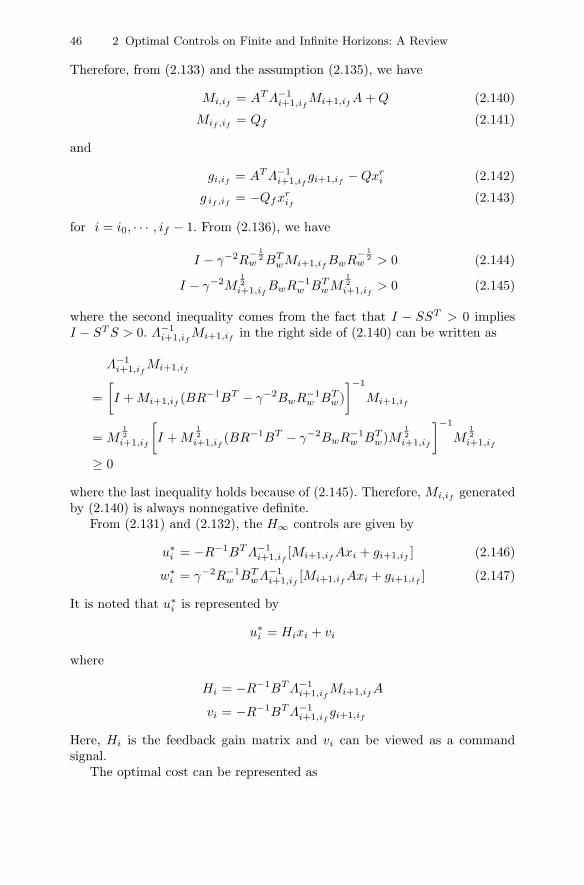
46 2 Optimal Controls on Finite and Infinite Horizons: A Review

Therefore, from (2.133) and the assumption (2.135), we have

Mi,if= AT Λ−1

i+1,ifMi+1,if

A + Q (2.140)

Mif ,if= Qf (2.141)

and

gi,if= AT Λ−1

i+1,ifgi+1,if

− Qxri (2.142)

g if ,if= −Qfxr

if(2.143)

for i = i0, · · · , if − 1. From (2.136), we have

I − γ−2R− 1

2w BT

wMi+1,ifBwR

− 12

w > 0 (2.144)

I − γ−2M12i+1,if

BwR−1w BT

wM12i+1,if

> 0 (2.145)

where the second inequality comes from the fact that I − SST > 0 impliesI − ST S > 0. Λ−1

i+1,ifMi+1,if

in the right side of (2.140) can be written as

Λ−1i+1,if

Mi+1,if

=[I + Mi+1,if

(BR−1BT − γ−2BwR−1w BT

w)]−1

Mi+1,if

= M12i+1,if

[I + M

12i+1,if

(BR−1BT − γ−2BwR−1w BT

w)M12i+1,if

]−1

M12i+1,if

≥ 0

where the last inequality holds because of (2.145). Therefore, Mi,ifgenerated

by (2.140) is always nonnegative definite.From (2.131) and (2.132), the H∞ controls are given by

u∗i = −R−1BT Λ−1

i+1,if[Mi+1,if

Axi + gi+1,if] (2.146)

w∗i = γ−2R−1

w BTwΛ−1

i+1,if[Mi+1,if

Axi + gi+1,if] (2.147)

It is noted that u∗i is represented by

u∗i = Hixi + vi

where

Hi = −R−1BT Λ−1i+1,if

Mi+1,ifA

vi = −R−1BT Λ−1i+1,if

gi+1,if

Here, Hi is the feedback gain matrix and vi can be viewed as a commandsignal.

The optimal cost can be represented as

2.3 Linear Optimal Control with State Feedback 47

J∗ = xTi Mi,if

xi + 2xTi gi,if

+ hi,if(2.148)

where Mi,ifand gi,if

are defined as (2.140) and (2.142) respectively. Thederivation for hi,if

is left as an exercise.The saddle-point value of the difference game with (2.128) for a zero ref-

erence signal is given as

J∗(xi, i, if ) = xTi Mi,if

xi (2.149)

Since Mi,ifis nonnegative definite, the saddle-point value (2.149) is nonneg-

ative.To conclude, the solution of the HTC problem can be reduced to finding

Mi,ifand gi,if

for i = i0, · · · , if − 1. The Riccati solution Mi,ifis a symmet-

ric matrix, which can be found by solving (2.140) backward in time using theboundary condition (2.141). In a similar manner, gi,if

can be found by solving(2.142) backward in time using the boundary condition (2.143).

For a regulation problem, i.e. xri = 0, the control (2.146) and the distur-

bance (2.147) can also be represented as[u∗

i

w∗i

]= −R−1

c,i

[BT

BTw

]Mi+1,if

Axi (2.150)

Mi,if= AT Mi+1,if

A − AT Mi+1,if

[B Bw

]R−1

c,i

[BT

BTw

]Mi+1,if

A

where

Rc,i =[

BT

BTw

]Mi+1,if

[B Bw

]+[

R 00 − γ2Rw

]It is observed that optimal solutions u∗ and w∗ in (2.150) look like an LQsolution.

For a positive definite Qf and a nonsingular matrix A, we can have anotherform of the control (2.146) and the disturbance (2.147). Let

Π = BR−1B − γ−2BwR−1w BT

w (2.151)

It is noted that Mi,ifis obtained from Ki,if

of the LQ control by replacingBR−1BT by Π. If Mi,if

is nonsingular at i ≤ if , then there exists the followingquantity:

Pi,if= M−1

i,if+ Π

In terms of Pi,if, (2.146) and (2.147) are represented as

u∗i = −R−1BT P−1

i+1,if[Axi + (Pi+1,if

− Π)gi+1,if] (2.152)

w∗i = γ−2R−1

w BTwP−1

i+1,if[Axi + (Pi+1,if

− Π)gi+1,if] (2.153)

48 2 Optimal Controls on Finite and Infinite Horizons: A Review

where

Pi,if= A−1Pi+1,if

[I + A−1QA−1Pi+1,if]−1A−1 + Π (2.154)

and

gi,if= −AT P−1

i+1,if(Pi+1,if

− Π)gi+1,if− Qxr

i (2.155)

with

Pif ,if= M−1

if ,if+ Π = Q−1

f + Π > 0, g if ,if= −Qfxr

if(2.156)

Here, Qf must be nonsingular.Note that P−1

i,ifis well defined only if Mi,if

satisfies the condition

Rw − γ−2BTwMi+1,if

Bw > 0 (2.157)

which is required for the existence of the saddle-point.

The terminal weighting matrix Qf cannot be arbitrarily large, since Mi,if

generated from the large Mif ,if= Qf is also large and thus the inequality

condition (2.136) may not be satisfied. That is why the terminal equality con-straint for case of the RH H∞ control does not make sense.

Infinite Horizon Case

From the finite horizon H∞ control of a form (2.150), we now turn to theinfinite horizon H∞ control, which is summarized in the following theorem.

Theorem 2.5. Suppose that (A,B) is stabilizable and (A,Q12 ) is observable.

For the infinite horizon performance criterion

infui

supwi

∞∑i=i0

[xT

i Qxi + uTi Rui − γ2wT

i Rwwi

](2.158)

the H∞ control and the worst-case disturbance are given by[u∗

i

w∗i

]= −R−1

c,∞

[BT

BTw

]M∞Axi

M∞ = AT M∞A − AT M∞[B Bw

]R−1

c,∞

[BT

BTw

]M∞A (2.159)

where

Rc,∞ =[

BT

BTw

]M∞

[B Bw

]+[

R 00 − γ2Rw

]if and only if the following conditions are satisfied:

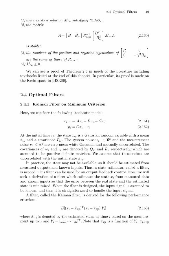
2.4 Optimal Filters 49

(1) there exists a solution M∞ satisfying (2.159);(2) the matrix

A −[B Bw

]R−1

c,∞

[BT

BTw

]M∞A (2.160)

is stable;

(3) the numbers of the positive and negative eigenvalues of[

R 00 − γ2Rw

]are the same as those of Rc,∞;

(4)M∞ ≥ 0.

We can see a proof of Theorem 2.5 in much of the literature includingtextbooks listed at the end of this chapter. In particular, its proof is made onthe Krein space in [HSK99].

2.4 Optimal Filters

2.4.1 Kalman Filter on Minimum Criterion

Here, we consider the following stochastic model:

xi+1 = Axi + Bui + Gwi (2.161)yi = Cxi + vi (2.162)

At the initial time i0, the state xi0 is a Gaussian random variable with a meanxi0 and a covariance Pi0 . The system noise wi ∈ p and the measurementnoise vi ∈ q are zero-mean white Gaussian and mutually uncorrelated. Thecovariances of wi and vi are denoted by Qw and Rv respectively, which areassumed to be positive definite matrices. We assume that these noises areuncorrelated with the initial state xi0 .

In practice, the state may not be available, so it should be estimated frommeasured outputs and known inputs. Thus, a state estimator, called a filter,is needed. This filter can be used for an output feedback control. Now, we willseek a derivation of a filter which estimates the state xi from measured dataand known inputs so that the error between the real state and the estimatedstate is minimized. When the filter is designed, the input signal is assumed tobe known, and thus it is straightforward to handle the input signal.

A filter, called the Kalman filter, is derived for the following performancecriterion:

E[(xi − xi|i)T (xi − xi|i)|Yi] (2.163)

where xi|j is denoted by the estimated value at time i based on the measure-ment up to j and Yi = [yi0 , · · · , yi]T . Note that xi|i is a function of Yi. xi+1|i

50 2 Optimal Controls on Finite and Infinite Horizons: A Review

and xi|i are often called a predictive estimated value and a filtered estimatedvalue respectively.

From Appendix C.1 we have the optimal filter

xi|i = E[xi|Yi] (2.164)

We first obtain a probability density function of xi given Yi and then find outthe mean of it.

By the definition of the conditional probability, we have

p(xi|Yi) =p(xi, Yi)

p(Yi)=

p(xi, yi, Yi−1)p(yi, Yi−1)

(2.165)

The numerator in (2.165) can be represented in terms of the conditional ex-pectation as follows:

p(xi, yi, Yi−1) = p(yi|xi, Yi−1)p(xi, Yi−1)= p(yi|xi, Yi−1)p(xi|Yi−1)p(Yi−1)= p(yi|xi)p(xi|Yi−1)p(Yi−1) (2.166)

where the last equality comes from the fact that Yi−1 is redundant informationif xi is given. Substituting (2.166) into (2.165) yields

p(xi|Yi) =p(yi|xi)p(xi|Yi−1)p(Yi−1)

p(yi, Yi−1)=

p(yi|xi)p(xi|Yi−1)p(Yi−1)p(yi|Yi−1)p(Yi−1)

=p(yi|xi)p(xi|Yi−1)

p(yi|Yi−1)(2.167)

For the given Yi, the denominator p(yi|Yi−1) is fixed. Two conditional prob-ability densities in the numerator of Equation (2.167) can be evaluated fromthe statistical information. For the given xi, yi follows the normal distribution,i.e. yi ∼ N (Cxi, Rv). The conditional probability p(xi|Yi−1) is also normal.Since E[xi|Yi−1] = xi|i−1 and E[(xi − xi|i−1)(xi − xi|i−1)T |Yi−1] = Pi|i−1,p(xi|Yi−1) is a normal probability function, i.e. N (xi|i−1, Pi|i−1). Therefore,we have

p(yi|xi) =1√

(2π)m|Rv|exp−1

2[yi − Cxi]T R−1

v [yi − Cxi]

p(xi|Yi−1) =1√

(2π)n|Pi|i−1|exp−1

2[xi − xi|i−1]T P−1

i|i−1[xi − xi|i−1]

from which, using (2.167), we find that

p(xi|Yi) = C exp−12[yi − Cxi]R−1

v [yi − Cxi] ×

exp−12[xi − xi|i−1]P−1

i|i−1[xi − xi|i−1] (2.168)

2.4 Optimal Filters 51

where C is the constant involved in the denominator of (2.167).We are now in a position to find out the mean of p(xi|Yi). Since the

Gaussian probability density function has a peak value at the average, we willfind xi that sets the derivative of (2.168) to zero. Thus, we can obtain thefollowing equation:

−2CT R−1v (yi − Cxi) + 2P−1

i|i−1(xi − xi|i−1) = 0 (2.169)

Denoting the solution xi to (2.169) by xi|i and arranging terms give

xi|i = (I + Pi|i−1CT R−1

v C)−1xi|i−1

+ (I + Pi|i−1CT R−1

v C)−1Pi|i−1CT R−1

v yi (2.170)

= [I − Pi|i−1CT (CPi|i−1C

T + Rv)−1C]xi|i−1

+ Pi|i−1CT (Rv + CPi|i−1C

T )−1yi (2.171)= xi|i−1 + Ki(yi − Cxi|i−1) (2.172)

where

Ki= Pi|i−1C

T (Rv + CPi|i−1CT )−1 (2.173)

xi+1|i can be easily found from the fact that

xi+1|i = E[xi+1|Yi] = AE[xi|Yi] + GE[wi|Yi] + Bui

= Axi|i + Bui (2.174)= Axi|i−1 + AKi(yi − Cxi|i−1) + Bui (2.175)

Pi+1|i can be obtained recursively from the error dynamic equations.Subtracting xi from both sides of (2.172) yields the following error equa-

tion:

xi|i = [I − KiC]xi|i−1 − Kivi (2.176)

where xi|i= xi|i − xi and xi|i−1 = xi|i−1 − xi. From (2.175) and (2.161), an

additional error equation is obtained as

xi+1|i = Axi|i − Gwi (2.177)

From (2.176) and (2.177), Pi|i and Pi+1|i are represented as

Pi|i = (I − KiC)Pi|i−1(I − KiC)T + KiRvKi = (I − KiC)Pi|i−1

Pi+1|i = APi|iAT + GQwGT

= APi|i−1AT + GQwGT

− APi|i−1CT (Rv + CPi|i−1C

T )−1CPi|i−1AT (2.178)

52 2 Optimal Controls on Finite and Infinite Horizons: A Review

The initial values xi0|i0−1 and Pi0|i0−1 are given by E[xi0 ] and E[(xi0 −xi0)(xi0 − xi0)

T ], which are a priori knowledge.The Kalman filter can be represented as follows:

xi+1|i = Axi|i−1 + APiCT (CPiC

T + Rv)−1(yi − Cxi|i−1) (2.179)

where

Pi+1 = APiAT − APiC

T (Rv + CPiCT )−1CPiA

T + GQwGT

= A[I + PiCT R−1

v C]−1PiAT + GQwGT (2.180)

with the given initial condition Pi0 . Note that Pi in (2.179) is used instead ofPi|i−1.

Throughout this book, we use the predicted form xi|i−1 instead of filteredform xi|i. For simple notation, xi|i−1 will be denoted by xi if necessary.

If the index i in (2.180) goes to ∞, then the infinite horizon or steady-stateKalman filter is given by

xi+1|i = Axi|i−1 + AP∞CT (CP∞CT + Rv)−1(yi − Cxi|i−1) (2.181)

where

P∞ = AP∞AT − AP∞CT (Rv + CP∞CT )−1CP∞AT + GQwGT

= A[I + P∞CT R−1v C]−1P∞AT + GQwGT (2.182)

As in LQ control, the following theorem gives the result on the conditionfor the existence of P∞ and the stability for the infinite horizon Kalman filter.

Theorem 2.6. If (A,G) is controllable and (A,C) is observable, then there isa unique positive definite solution P∞ to the ARE (2.182). Additionally, thesteady-state Kalman filter is asymptotically stable.

We can see a proof of Theorem 2.6 in much of the literature includingtextbooks listed at the end of this chapter. In Theorem 2.6, the conditionson controllability and observability can be weakened to the reachability anddetectability.

2.4.2 H∞ Filter on Minimax Criterion

Here, an H∞ filter is introduced. Consider the following systems:

xi+1 = Axi + Bwwi + Bui

yi = Cxi + Dwwi

zi = Czx(2.183)

where xi ∈ n denotes states, wi ∈ l disturbance, ui ∈ m inputs, yi ∈ p

measured outputs, and zi ∈ q estimated values. BwDTw = 0 and DwDT

w =

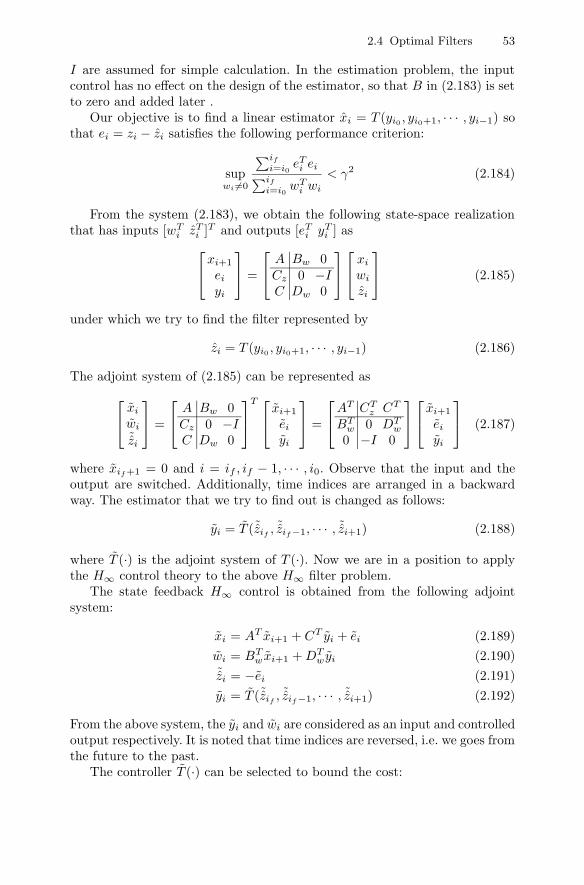
2.4 Optimal Filters 53

I are assumed for simple calculation. In the estimation problem, the inputcontrol has no effect on the design of the estimator, so that B in (2.183) is setto zero and added later .

Our objective is to find a linear estimator xi = T (yi0 , yi0+1, · · · , yi−1) sothat ei = zi − zi satisfies the following performance criterion:

supwi =0

∑if

i=i0eT

i ei∑if

i=i0wT

i wi

< γ2 (2.184)

From the system (2.183), we obtain the following state-space realizationthat has inputs [wT

i zTi ]T and outputs [eT

i yTi ] as⎡⎣xi+1

ei

yi

⎤⎦ =

⎡⎣ A Bw 0Cz 0 −IC Dw 0

⎤⎦⎡⎣ xi

wi

zi

⎤⎦ (2.185)

under which we try to find the filter represented by

zi = T (yi0 , yi0+1, · · · , yi−1) (2.186)

The adjoint system of (2.185) can be represented as⎡⎣ xi

wi

˜zi

⎤⎦ =

⎡⎣ A Bw 0Cz 0 −IC Dw 0

⎤⎦T ⎡⎣ xi+1

ei

yi

⎤⎦ =

⎡⎣AT CTz CT

BTw 0 DT

w

0 −I 0

⎤⎦⎡⎣ xi+1

ei

yi

⎤⎦ (2.187)

where xif+1 = 0 and i = if , if − 1, · · · , i0. Observe that the input and theoutput are switched. Additionally, time indices are arranged in a backwardway. The estimator that we try to find out is changed as follows:

yi = T (˜zif, ˜zif−1, · · · , ˜zi+1) (2.188)

where T (·) is the adjoint system of T (·). Now we are in a position to applythe H∞ control theory to the above H∞ filter problem.

The state feedback H∞ control is obtained from the following adjointsystem:

xi = AT xi+1 + CT yi + ei (2.189)wi = BT

w xi+1 + DTw yi (2.190)

˜zi = −ei (2.191)yi = T (˜zif

, ˜zif−1, · · · , ˜zi+1) (2.192)

From the above system, the yi and wi are considered as an input and controlledoutput respectively. It is noted that time indices are reversed, i.e. we goes fromthe future to the past.

The controller T (·) can be selected to bound the cost:

54 2 Optimal Controls on Finite and Infinite Horizons: A Review

max‖ei‖2,[0,if ] =0

∑if

i=i0wT

i wi∑if

i=i0eT

i ei

< γ2 (2.193)

According to (2.146) and the correspondence

Q ←− BwBTw , R ←− I, Rw ←− I, AT ←− A, B ←− CT , Bw ←− Cz

the resulting controller and the worst case ei are given:

yi = −LTi,i0 xi+1, ei = −NT

i,i0 xi+1 (2.194)

where

LTi,i0 = CΓ−1

i,i0Si,i0A

T , NTi,i0 = −CzΓ

−1i,i0

Si,i0AT (2.195)

Si+1,i0 = ASi,i0Γ−1i,i0

AT + BwBTw (2.196)

Γi,i0 = I + (CT C − γ−2CTz Cz)Si,i0 (2.197)

with Si0,i0 = 0. In Figure 2.6, controls using Riccati solutions are representedin forward and backward ways. The state-space model for the controller isgiven as

xi = AT xi+1 − CT LTi,i0 xi+1 + CT

z ei (2.198)

yi = −LTi,if

xi+1, (2.199)

which can be represented as[xi

yi

]=[

AT − CT LTi,i0

CTz

−LTi,i0

0

] [xi+1

ei

]=[

AT − CT LTi,i0

−CTz

−LTi,i0

0

] [xi+1

˜zi

](2.200)

Forward way

Backward way

Fig. 2.6. Computation directions for H∞ filter

2.4 Optimal Filters 55

which is a state-space realization for the control (2.188). The adjoint systemof (2.200) is as follows:[

ηi+1

zi

]=[

AT − CT LTi,i0

− CTz

−LTi,i0

0

]T [ηi

yi

]=[

A − Li,i0C − Li,i0

−Cz 0

] [ηi

yi

]which is a state-space realization for the filter (2.186). Rearranging terms,replacing −ηi with xi, and adding the input into the estimator equation yieldsthe H∞ filter

zi = Czxi, xi+1 = Axi + Bui + Li,i0(yi − Cxi) (2.201)

The H∞ filter can also be represented as follows:

zi = Czxi, xi+1 = Axi + ASi,i0

[CT CT

z

]R−1

f,i

[y − Cxi

0

](2.202)

Si+1,i0 = ASi,i0AT − ASi,i0

[CT CT

z

]R−1

f,i

[CCz

]Si,i0A

T + BwBTw (2.203)

where

Rf,i =[

Ip 00 − γ2Iq

]+[

CCz

]Si,i0

[CT CT

z

]It is observed that the H∞ filter of the form (2.202) and (2.203) looks like theKalman filter.

From the finite horizon H∞ filter of the form (2.202) and (2.203), we nowturn to the infinite horizon H∞ filter. If the index i goes to ∞, the infinitehorizon H∞ filter is given by

zi = Czxi, xi+1 = Axi + AS∞[CT CT

z

]R−1

f,∞

[y − Cxi

0

](2.204)

S∞ = AS∞AT − AS∞[CT CT

z

]R−1

f,∞

[CCz

]S∞AT + BwBT

w (2.205)

where

Rf,∞ =[

Ip 00 − γ2Iq

]+[

CCz

]S∞[CT CT

z

](2.206)

As in the infinite horizon H∞ control, the following theorem gives the resulton the condition for the existence of S∞ and stability for the infinite horizonH∞ filter.

Theorem 2.7. Suppose that (A,B) is stabilizable and (A,Q12 ) is observable.

For the following infinite horizon performance criterion:

maxwi =0

∑∞i=i0

eTi ei∑∞

i=i0wT

i wi< γ2 (2.207)

the H∞filter (2.204) exists if and only if the following things are satisfied:

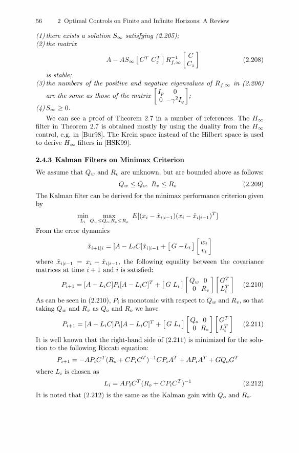
56 2 Optimal Controls on Finite and Infinite Horizons: A Review

(1) there exists a solution S∞ satisfying (2.205);(2) the matrix

A − AS∞[CT CT

z

]R−1

f,∞

[CCz

](2.208)

is stable;(3) the numbers of the positive and negative eigenvalues of Rf,∞ in (2.206)

are the same as those of the matrix[

Ip 00 −γ2Iq

];

(4)S∞ ≥ 0.

We can see a proof of Theorem 2.7 in a number of references. The H∞filter in Theorem 2.7 is obtained mostly by using the duality from the H∞control, e.g. in [Bur98]. The Krein space instead of the Hilbert space is usedto derive H∞ filters in [HSK99].

2.4.3 Kalman Filters on Minimax Criterion

We assume that Qw and Rv are unknown, but are bounded above as follows:

Qw ≤ Qo, Rv ≤ Ro (2.209)

The Kalman filter can be derived for the minimax performance criterion givenby

minLi

maxQw≤Qo,Rv≤Ro

E[(xi − xi|i−1)(xi − xi|i−1)T ]

From the error dynamics

xi+1|i = [A − LiC]xi|i−1 +[G −Li

] [wi

vi

]where xi|i−1 = xi − xi|i−1, the following equality between the covariancematrices at time i + 1 and i is satisfied:

Pi+1 = [A − LiC]Pi[A − LiC]T +[G Li

] [Qw 00 Rv

] [GT

LTi

](2.210)

As can be seen in (2.210), Pi is monotonic with respect to Qw and Rv, so thattaking Qw and Rv as Qo and Ro we have

Pi+1 = [A − LiC]Pi[A − LiC]T +[G Li

] [Qo 00 Ro

] [GT

LTi

](2.211)

It is well known that the right-hand side of (2.211) is minimized for the solu-tion to the following Riccati equation:

Pi+1 = −APiCT (Ro + CPiC

T )−1CPiAT + APiA

T + GQoGT

where Li is chosen as

Li = APiCT (Ro + CPiC

T )−1 (2.212)

It is noted that (2.212) is the same as the Kalman gain with Qo and Ro.

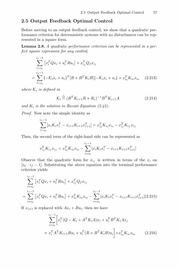
2.5 Output Feedback Optimal Control 57

2.5 Output Feedback Optimal Control

Before moving to an output feedback control, we show that a quadratic per-formance criterion for deterministic systems with no disturbances can be rep-resented in a square form.

Lemma 2.8. A quadratic performance criterion can be represented in a per-fect square expression for any control,

if−1∑i=i0

[xT

i Qxi + uTi Rui

]+ xT

ifQfxif

=if−1∑i=i0

−Kixi + uiT [R + BT KiB]−Kixi + ui + xTi0Ki0xi0 (2.213)

where Ki is defined in

Ki= (BT Ki+1B + Rv)−1BT Ki+1A (2.214)

and Ki is the solution to Riccati Equation (2.45).

Proof. Now note the simple identity as

if−1∑i=i0

[xiKixTi − xi+1Ki+1x

Ti+1] = xT

i0Ki0xi0 − xTif

Kifxif

Then, the second term of the right-hand side can be represented as

xTif

Kifxif

= xTi0Ki0xi0 −

if−1∑i=i0

[xiKixTi − xi+1Ki+1x

Ti+1]

Observe that the quadratic form for xifis written in terms of the xi on

[i0 if − 1]. Substituting the above equation into the terminal performancecriterion yields

if−1∑i=i0

[xT

i Qxi + uTi Rui

]+ xT

ifQfxif

=if−1∑i=i0

[xT

i Qxi + uTi Rui

]+ xT

i0Ki0xi0 −if−1∑i=i0

[xiKixTi − xi+1Ki+1x

Ti+1](2.215)

If xi+1 is replaced with Axi + Bui, then we have

if−1∑i=i0

[xT

i (Q − Ki + AT KiA)xi + uTi BT KiAxj

+ xTi AT Ki+1Bui + uT

i (R + BT KiB)ui

]+xT

i0Ki0xi0 (2.216)

58 2 Optimal Controls on Finite and Infinite Horizons: A Review

If Ki satisfies (2.45), then the square completion is achieved as (2.213), Thiscompletes the proof.

2.5.1 Linear Quadratic Gaussian Control on Minimum Criterion

Now, we introduce an output feedback LQG control. A quadratic performancecriterion is given by

J =if−1∑i=i0

E

[xT

i Qxi + uTi Rui

∣∣∣∣yi−1, yi−2, · · · , yi0

]

+ E

[xT

ifQfxif

∣∣∣∣yif−1, yif−2, · · · , yi0

](2.217)

subject to ui = f(yi−1, · · · , yi0). Here, the objective is to find a controller ui

that minimizes (2.217). From now on we will not include the condition partinside the expectation for simplicity. Before obtaining the LQG control, asin the deterministic case (2.213), it is shown that the performance criterion(2.217) can be represented in a square form.Lemma 2.9. A quadratic performance criterion can be represented in a per-fect square expression for any control,

E

[if−1∑i=i0

[xT

i Qxi + uTi Rui

]+ xT

ifQfxif

]

= E

[if−1∑i=i0

−Kixi + uiT [R + BT KiB]−Kixi + ui]

+ tr[ if−1∑

i=i0

KiGQwGT]+ E

[xT

i0Ki0xi0

](2.218)

where Ki is defined in

Ki= (BT Ki+1B + R)−1BT Ki+1A (2.219)

and Ki is the solution to Riccati Equation (2.45).

Proof. The relation (2.215) holds even for stochastic systems (2.161)-(2.162).Taking an expectation on (2.215), we have

E

[if−1∑i=i0

[xT

i Qxi + uTi Rui

]+ xT

ifQfxif

]

= E

[if−1∑i=i0

[xT

i Qxi + uTi Rui

]+ xT

i0Ki0xi0

−if−1∑i=i0

[xiKixTi − xi+1Ki+1x

Ti+1]]

(2.220)

2.5 Output Feedback Optimal Control 59

Replacing xi+1 with Axi + Bui + Gwi yields

E

[if−1∑i=i0

[xT

i (Q − Ki + AT KiA)xi + uTi BT KiAxj

+ xTi AT Ki+1Bui + uT

i (R + BT KiB)ui

]]+E

[xT

i0Ki0xi0

]

+ tr[if−1∑

i=i0

KiGQwGT

](2.221)

If Ki satisfies (2.140), then the square completion is achieved as (2.218). Thiscompletes the proof.

Using Lemma 2.9, we are now in a position to represent the performancecriterion (2.217) in terms of the estimated state. Only the first term in (2.221)is dependent on ui. So, we consider only this term. Let xi|i−1 be denoted byxi|i−1 = E[xi|yi−1, yi−2, · · · , yi0 ]. According to (C.2) in Appendix C, we canchange the first term in (5.69) to

E

if−1∑i=i0

(Kixi + ui)T Ri(Kixi + ui) =if−1∑i=i0

(Kixi + ui)T Ri(Kixi + ui)

+ trif∑

i=i0+1

R12i KiPiKT

i R12i (2.222)

where

Ri= R + BT KiB (2.223)

and Pi is the variance between xi|i−1 and xi. Note that Kixi|i−1 + ui =

E[Kixi + ui | yi−1, yi−2, · · · , yi0 ] and tr(RiKiPiKTi ) = tr(R

12i KiPiKT

i R12i ).

We try to find the optimal filter gain Li making the following filter mini-mizing Pi:

xi+1|i = Axi|i−1 + Li(yi − Cxi|i−1) + Bui (2.224)

Subtracting (2.161) from (2.224), we have

xi+1|i = xi+1|i − xi+1 = (A − LiC)xi|i−1 + Livi − Gwi (2.225)

which leads to the following equation:

Pi+1 = (A − LiC)Pi(A − LiC)T + LiRvLTi + GQwGT (2.226)

where Pi is the covariance of xi|i−1. As can be seen in (2.226), Pi is indepen-dent of ui, so that Pi and ui can be determined independently. Pi+1 in (2.226)can be written as

60 2 Optimal Controls on Finite and Infinite Horizons: A Review

Pi+1 =[Li(CPiC

T + Rv) − APi

](CPiC

T + R)−1

[Li(CPiC

T + Rv) − APi

]T

+ GQwGT + APi(CPiCT + Rv)−1PiA

T

≥ GQwGT + APi(CPiCT + Rv)−1PiA

T (2.227)

where the equality holds if Li = APiCT (Rv + CPiC

T )−1.It can be seen in (2.227) that the covariance Pi generated by the Kalman

filter is optimal in view that the covariance Pi of any linear estimator islarger than Pi of the Kalman filter, i.e. Pi ≤ Pi. This implies that tr(Pi) ≤tr(Pi), leading to tr(R

12i KiPiK

Ti R

12i ) ≤ tr(R

12i KiPiK

Ti R

12i ). Thus, the xi|i−1

minimizing (2.222) is given by the Kalman filter as follows:

xi+1|i = Axi|i−1 + [APiCT (Rv + CPiC

T )−1](yi − Cxi|i−1) + Bui (2.228)

Pi+1 = GQwGT + APi(CPiCT + Rv)−1PiA

T (2.229)

with the initial state mean xi0 and the initial covariance Pi0 . Thus, the fol-lowing LQG control minimizes the performance criterion:

u∗i = −(BT Ki+1B + R)−1BT Ki+1Axi|i−1 (2.230)

Infinite Horizon Linear Quadratic Gaussian Control

We now turn to the infinite horizon LQG control. It is noted that, as thehorizon N gets larger, (2.217) also becomes larger and finally blows up. So,the performance criterion (2.217) cannot be applied as it is to the infinitehorizon case. In a steady state for the infinite horizon case, we may write

minui

J = minui

E[xTi Qxi + uT

i Rui] (2.231)

= minui

12π

∫ 2π

0

tr(T (ejω)T ∗(ejω)) dω (2.232)

where T (ejω) is the transfer function from wi and vi to ui and xi. The infinitehorizon LQG control is summarized in the following theorem.

Theorem 2.10. Suppose that (A,B) and (A,G) are controllable and (A,Q12 )

and (A,C) are observable. For the infinite horizon performance criterion(2.232), the infinite horizon LQG control is given by

u∗i = −(BT K∞B + R)−1BT K∞Axi|i−1 (2.233)

where

K∞ = AT K∞A − AT K∞B[R + BK∞BT ]−1BT K∞A + Q

xi+1|i = Axi|i−1 + [AP∞CT (Rv + CP∞CT )−1](yi − Cxi|i−1) + Bui

P∞ = GQwGT + AP∞(CP∞CT + Rv)−1P∞AT

2.5 Output Feedback Optimal Control 61

We can see a proof of Theorem 2.10 in many references, e.g. in [Bur98,Lew86b]. The conditions on controllability and observability in Theorem 2.10can be weakened to the reachability and detectability.

2.5.2 Output Feedback H∞ Control on Minimax Criterion

Now, we derive the output feedback H∞ control. The result of the previousH∞ filter will be used to obtain the output feedback H∞ control. First, theperformance criterion is transformed in perfect square forms with respect tothe optimal control and disturbance.

Lemma 2.11. H∞ performance criterion can be represented in a perfectsquare expression for arbitrary control.

if−1∑i=i0

[xT

i Qxi + uTi Rui − γ2wT

i Rwwi

]+xT

ifQfxif

=if−1∑i=i0

[(ui − u∗

i )TVi(ui − u∗

i ) − γ2(wi − w∗i )TWi(wi − w∗

i )]

+ xTi0Mi0xi0 (2.234)

where w∗i and u∗

i are given as

w∗i = (γ2Rw − BT

wMi+1Bw)−1BTwMi+1(Axi + Bui) (2.235)

u∗i = −R−1BT Mi+1[I + (BR−1BT − γ−2BwR−1

w BTw)Mi+1]−1Axi (2.236)

Vi = R + BT Mi+1(I − γ−2BwR−1w BT

wMi+1)−1B

Wi = γ2Rw − BTwMi+1Bw

and Mi shortened for Mi,ifis given in (2.140).

Proof. Recalling the simple identity as

if−1∑i=i0

[xiMixTi − xi+1Mi+1x

Ti+1] = xT

i0Mi0xi0 − xTif

Mifxif

we have

xTif

Mifxif

= xTif

Qfxif= xT

i0Mi0xi0 −if−1∑i=i0

[xTi Mixi − xT

i+1Mi+1xi+1] (2.237)

By substituting (2.237) into the final cost xTif

Qfxif, the H∞ performance

criterion of the left-hand side in (2.234) can be changed as

62 2 Optimal Controls on Finite and Infinite Horizons: A Review

if−1∑i=i0

[xT

i Qxi + uTi Rui − γ2wT

i Rwwi

]+ xT

ifQfxif

=if−1∑i=i0

[xT

i Qxi + uTi Rui − γ2wT

i Rwwi

]+ xT

i0Mi0xi0

−if−1∑i=i0

[xTi Mixi − xT

i+1Mi+1xi+1]

=if−1∑i=i0

[xT

i Qxi + uTi Rui − γ2wT

i Rwwi − xTi Mixi

+ xTi+1Mi+1xi+1

]+xT

i0Mi0xi0 (2.238)

Now, we try to make terms inside the summation represented in a perfectsquare form. First, time variables are all changed to i. Next, we complete thesquare with respect to wi and ui respectively.

Terms in the summation (2.238) can be arranged as follows:

xTi+1Mi+1xi+1 − xT

i Mixi + xTi Qxi + uT

i Rui − γ2wTi Rwwi

+ xTi Qxi + uT

i Rui − γ2wTi Rwwi

= ATo,iMi+1Ao,i + wT

i BTwMi+1Ao,i + AT

o,iMi+1Bwwi

− wTi (γ2Rw − BT

wMi+1Bw)wi + xTi (−Mi + Q)xi + uT

i Rui (2.239)

where Ao,i = Axi + Bui. Terms including wi in (2.239) can be arranged as

wTi BT

wMi+1Ao,i + ATo,iMi+1Bwwi − wT

i (γ2Rw − BTwMi+1Bw)wi

= −WTi (γ2Rw − BT

wMi+1Bw)−1Wi

+ ATo,iMi+1Bw(γ2Rw − BT

wMi+1Bw)−1BTwMi+1Ao,i (2.240)

where Wi = (γ2Rw − BTwMi+1Bw)wi − BT

wMi+1Ao,i. After completing thesquare with respect to disturbance wi, we try to do that for the control ui.Substituting (2.240) into (2.239) yields

−WTi (γ2Rw − BT

wMi+1Bw)−1Wi

+ ATo,iMi+1Bw(γ2Rw − BT

wMi+1Bw)−1BTwMi+1Ao,i

+ ATo,iMi+1Ao,i + xT

i (−Mi + Q)xi + uTi Rui

= −WTi (γ2Rw − BT

wMi+1Bw)−1Wi + ATo,iMi+1(I − γ−2BwR−1

w BTwMi+1)−1

× Ao,i + xTi (−Mi + Q)xi + uT

i Rui (2.241)

where the last equality comes from

P (I − RQ−1RT P )−1 = P + PR(Q − RT PR)−1RT P

2.5 Output Feedback Optimal Control 63

for some matrix P , R, and Q.The second, the third, and the fourth terms in the right-hand side of

(2.241) can be factorized as

(Axi + Bui)T Mi+1Z−1i (Axi + Bui) + xT

i (−Mi + Q)xi + uTi Rui

= uTi [R + BT Mi+1Z−1

i B]ui + uTi BT Mi+1Z−1

i Axi + xTi AT Mi+1Z−1

i Bui

+ xTi [AT Mi+1Z−1

i A − Mi + Q]xi = UTi

[R + BT Mi+1Z−1

i B]−1

Ui (2.242)

where

Ui =[R + BT Mi+1Z−1

i B]ui + BT Mi+1Z−1

i Axi

Zi = I − γ−2BwR−1w BT

wMi+1

and the second equality comes from the Riccati equation represented by

Mi = AT Mi+1(I + (BR−1BT − γ−2BwR−1w BT

w)Mi+1)−1A + Q

= AT Mi+1(Zi + BR−1BT Mi+1)−1A + Q

= AT Mi+1

[Z−1

i −Z−1i BR−1BT (Mi+1Z−1

i BR−1BT + I)−1Mi+1Z−1i

]A

+ Q

or

AT Mi+1Z−1i A − Mi + Q

= AT Mi+1Z−1i BR−1BT (Mi+1Z−1

i BR−1BT + I)−1Mi+1Z−1i A

= AT Mi+1Z−1i B(BT Mi+1Z−1

i B + R)−1BT Mi+1Z−1i A

This completes the proof.

Note that by substituting (5.154) into (5.153), w∗i can be represented as

w∗i = γ−2R−1

w BTwMi+1[I + (BR−1BT − γ−2BwR−1

w BTw)Mi+1]−1Axi

which is of very similar form to u∗i .

For the zero initial state, the inequality

if−1∑i=i0

[xT

i Qxi + uTi Rui − γ2wT

i Rwwi

]+xT

ifQfxif

< 0 (2.243)

guarantees the bound on the following ∞ norm:

sup‖wi‖2,[0,if ] =0

∑if−1i=i0

(ui − u∗i )

TVi(ui − u∗i )∑if−1

i=i0(wi − w∗

i )TWi(wi − w∗i )

< γ2 (2.244)

where u∗i and w∗

i are defined in (5.154) and (5.153) respectively. Here, Rw = I,DwBT

w = 0, and DwDTw = I are assumed for simple calculation.

64 2 Optimal Controls on Finite and Infinite Horizons: A Review

According to (2.244), we should design ui so that the H∞ norm betweenthe weighted disturbance deviation

wi= W

12i wi −W

12i (γ2I − BT

wMi+1Bw)−1BTwMi+1(Axi + Bui)

and the weighted control deviation

ui= V

12i ui + V

12i R−1BT Mi+1[I + (BR−1BT − γ−2BwBT

w)Mi+1]−1Axi

is minimized. By using wi, we obtain the following state-space model:

xi+1 = Aa,ixi + Ba,iui + BwW− 1

2i wi

yi = Cxi + DwW− 1

2i wi (2.245)

where Aa,i = A + Bw(γ2I − BTwMi+1Bw)−1BT

wMi+1A, and Ba,i = B +Bw(γ2I − BT

wMi+1Bw)−1BTwMi+1B. Note that DwBT

w = 0 is assumed asmentioned before.

The performance criterion (2.244) for the state-space model (2.245) is justone for the H∞ filter that estimates u∗

i with respect to wi by using mea-surements yi. This is a similar structure to (2.183). Note that the variable zi

in (2.183) to be estimated corresponds to u∗i . Using the result of H∞ filters,

we can think of this as finding out the output feedback H∞ control ui byobtaining the estimator of u∗

i .All derivations require long and tedious algebraic calculations. In this

book, we just summarize the final result. The output feedback H∞ controlis given by

ui = −Kof,ixi

Kof,i = R−1BT Mi+1[I + (BR−1BT − γ−2BwBTw)Mi+1]−1A

xi+1 = Aa,ixi + Lof,i

[0

yi − Cxi

]+ Bui

where Mi, i.e. Mi,if, is given in (2.140) and Lof,i is defined as

Lof,i =(

Aa,iSof,i

[−KT

of,i CT]− γ2Bw

[Si 0

])R−1

of,i

Sof,i+1 = Aa,iSof,iATa,i − γ2BwW−1

i BTw − Lof,iRof,iL

Tof,i

Rof,i =[−γ2Z−1

i 00 I

]+[−Kof,i

C

]Sof,i

[−KT

of,i CT]

[W−1

i Si

STi Z−1

i

]=([

−γ2I 00 R

]+[

BTw

BT

]Mi+1

[Bw B

])−1

with the initial conditions Mif ,if= Qf and Si0 = 0.

2.5 Output Feedback Optimal Control 65

Infinite Horizon Output Feedback H∞ Control

Now we introduce the infinite horizon H∞ output feedback control in thefollowing theorem:

Theorem 2.12. Infinite horizon H∞ output feedback control is composed of

ui = −Kof,∞xi

Kof,∞ = R−1BT M∞[I + (BR−1BT − γ−2BwBTw)M∞]−1A

xi+1 = Aa,∞xi + Lof,∞

[yi − Cxi

0

]+ Bui

where

Aa,∞ = A + Bw(γ2I − BTwM∞Bw)−1BT

wM∞A

Lof,∞ =(

Aa,∞Sof,∞[−KT

of,∞ CT]− γ2Bw

[S∞ 0

])R−1

of,∞

Sof,∞ = Aa,∞Sof,∞ATa,∞ − γ2BwW−1

∞ BTw − Lof,∞Rof,∞LT

of,∞

Rof,∞ =[−γ2(Z∞)−1 0

0 Ip

]+[−Kof,∞

C

]Pi

[−KT

of,∞ CT]

[W−1

∞ S∞ST∞ Z−1

∞

]=([

−γ2Il 00 R

]+[

BTw

BT

]M∞

[Bw B

])−1

and achieves the following specification∑∞i=i0

xTi Rxi + uT

i Qui∑∞i=i0

wTi wi

< γ2

if and only if there exists solutions M∞ ≥ 0 satisfying (2.159) and Sof,∞ ≥ 0such that

(1)A−[B Bw

]([R 00 −γ2I

]+[

BT

BTw

]M∞

[B Bw

])−1[BT

BTw

]M∞A is stable.

(2)The numbers of the positive and negative eigenvalues of the two followingmatrices are the same:[

R 00 −γ2Il

],

[R 00 −γ2Il

]+[

BT

BTw

]M∞

[B Bw

](2.246)

(3)Aa,∞ − Lof,∞

[C

(I + BT M∞B)12 Kof,∞

]is stable.

(4)The numbers of the positive and negative eigenvalues of[

Ip 00 −γ2Im

]are

the same as those of the following matrix:[Ip 00 −γ2Im + T

]+[

C

X12 Kof,∞

]Sof,∞

[CT KT

of,∞X12

](2.247)

66 2 Optimal Controls on Finite and Infinite Horizons: A Review

where T = X− 12 BT M∞Z−1M∞BX− 1

2 , Z = I−BT M∞(I+BBT M∞)−1B,and X = I + BT M∞B.

We can see a proof of Theorem 2.12 in [HSK99]. It is shown in [Bur98] thatoutput feedback H∞ control can be obtained from a solution to an estimationproblem.

2.6 Linear Optimal Controls via Linear MatrixInequality

In this section, optimal control problems for discrete linear time-invariantsystems are reformulated in terms of linear matrix inequalities (LMIs). SinceLMI problems are convex, it can be solved very efficiently and the globalminimum is always found. We first consider the LQ control and then move toH∞ control.

2.6.1 Infinite Horizon Linear Quadratic Control via Linear MatrixInequality

Let us consider the infinite horizon LQ cost function as follows:

J∞ =∞∑

i=0

xT

i Qxi + uTi Rui

,

where Q > 0, R > 0. It is noted that, unlike the standard LQ control, Q ispositive-definite. The nonsingularity of Q is required to solve an LMI problem.We aim to find the control ui which minimizes the above cost function. Themain attention is focused on designing a linear optimal state-feedback control,ui = Hxi. Assume that V (xi) has the form

V (xi) = xTi Kxi, K > 0

and satisfies the following inequality:

V (xi+1) − V (xi) ≤ −[xTi Qxi + uT

i Rui] (2.248)

Then, the system controlled by ui is asymptotically stable and J∞ ≤ V (x0).With ui = Hxi, the inequality (2.248) is equivalently rewritten as

xTi (A + BH)T K(A + BH)xi − xT

i Kxi ≤ −xTi [Q + HT RH]xi (2.249)

From (2.249), it is clear that (2.248) is satisfied if there exists H and K suchthat

(A + BH)T K(A + BH) − K + Q + HT RH ≤ 0 (2.250)

2.6 Linear Optimal Controls via Linear Matrix Inequality 67

Instead of directly minimizing xT0 Kx0, we take an approach where its upper

bound is minimized. For this purpose, assume that there exists γ2 > 0 suchthat

xT0 Kx0 ≤ γ2 (2.251)

Now the optimal control problem for given x0 can be formulated as follows:

minγ2,K,H

γ2 subject to (2.250) and (2.251)

However, the above optimization problem does not seem easily solvable be-cause the matrix inequalities (2.250) and (2.251) are not of LMI forms. In thefollowing, matrix inequalities (2.250) and (2.251) are converted to LMI con-ditions. First, let us turn to the condition in (2.250), which can be rewrittenas follows:

−K +[(A + BH)T HT I

] ⎡⎣K−1 0 00 R−1 00 0 Q−1

⎤⎦−1 ⎡⎣ (A + BH)HI

⎤⎦ ≤ 0

From the Schur complement, the above inequality is equivalent to⎡⎢⎢⎣−K (A + BH)T HT I

(A + BH) −K−1 0 0H 0 −R−1 0I 0 0 −Q−1

⎤⎥⎥⎦ ≤ 0 (2.252)

Also from the Schur complement, (2.251) is converted to[γ2 xT

0

x0 K−1

]≥ 0 (2.253)

Pre- and post-multiply (2.252) by diagK−1, I, I, I. It should be notedthat this operation does not change the inequality sign. Introducing new vari-ables Y HK−1 and S K−1, (2.252) is equivalently changed into⎡⎢⎢⎣

−S (AS + BY )T Y T S(AS + BY ) −S 0 0

Y 0 −R−1 0S 0 0 −Q−1

⎤⎥⎥⎦ ≤ 0 (2.254)

Furthermore, (2.253) is converted to[γ2 xT

0

x0 S

]≥ 0 (2.255)

Now that (2.254) and (2.255) are LMI conditions, the resulting optimizationproblem is an infinite horizon control, which is represented as follows:

minγ2,Y,S

γ2

subject to (2.254) and (2.255)

Provided that the above optimization problem is feasible, then H = Y S−1

and K = S−1.

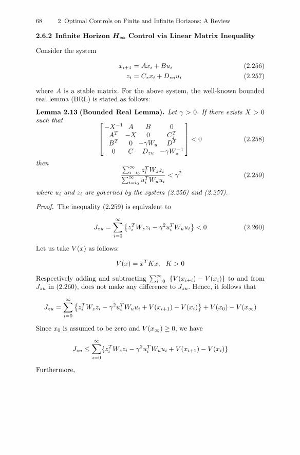
68 2 Optimal Controls on Finite and Infinite Horizons: A Review

2.6.2 Infinite Horizon H∞ Control via Linear Matrix Inequality

Consider the system

xi+1 = Axi + Bui (2.256)zi = Czxi + Dzuui (2.257)

where A is a stable matrix. For the above system, the well-known boundedreal lemma (BRL) is stated as follows:

Lemma 2.13 (Bounded Real Lemma). Let γ > 0. If there exists X > 0such that ⎡⎢⎢⎣

−X−1 A B 0AT −X 0 CT

z

BT 0 −γWu DT

0 C Dzu −γW−1z

⎤⎥⎥⎦ < 0 (2.258)

then ∑∞i=i0

zTi Wzzi∑∞

i=i0uT

i Wuui< γ2 (2.259)

where ui and zi are governed by the system (2.256) and (2.257).

Proof. The inequality (2.259) is equivalent to

Jzu =∞∑

i=0

zT

i Wzzi − γ2uTi Wuui

< 0 (2.260)

Let us take V (x) as follows:

V (x) = xT Kx, K > 0

Respectively adding and subtracting∑∞

i=0 V (xi+i) − V (xi) to and fromJzu in (2.260), does not make any difference to Jzu. Hence, it follows that

Jzu =∞∑

i=0

zT

i Wzzi − γ2uTi Wuui + V (xi+1) − V (xi)

+ V (x0) − V (x∞)

Since x0 is assumed to be zero and V (x∞) ≥ 0, we have

Jzu ≤∞∑

i=0

zTi Wzzi − γ2uT

i Wuui + V (xi+1) − V (xi)

Furthermore,

2.6 Linear Optimal Controls via Linear Matrix Inequality 69

∞∑i=0

zTi Wzzi − γ2uT

i Wuui + V (xi+1) − V (xi)

=∞∑

i=0

[Czxi + Dzuui]T Wz[Czxi + Dzuui] − γ2uT

i Wuui

+[Axi + Bui]T K[Axi + Bui] − xTi Kxi

=

∞∑i=0

[xi

ui

]T

Λ

[xi

ui

]

where

Λ [−K + AT KA + CT

z WzCz AT KB + CTz WzDzu

BT KA + DTzuWzCz BT KB + DT

zuWzDzu − γ2Wu

](2.261)

Hence, if the 2-by-2 block matrix Λ in (2.261) is negative definite, then Jzu < 0and equivalently the inequality (2.259) holds.

The 2-by-2 block matrix Λ can be rewritten as follows:

Λ =[−K 00 −γ2Wu

]+[

AT CTz

BT DTzu

] [K 00 Wz

] [A BCz Dzu

]From the Schur complement, the negative definiteness of Λ is guaranteed ifthe following matrix equality holds:⎡⎢⎢⎣

−K 0 AT CTz

0 −γ2Wu BT DTzu

A B −K−1 0Cz Dzu 0 −W−1

z

⎤⎥⎥⎦ < 0 (2.262)

Define Π as follows:

Π

⎡⎢⎢⎣0 I 0 00 0 I 0I 0 0 00 0 0 I

⎤⎥⎥⎦Pre- and post-multiplying (2.262) by ΠT and Π respectively does not changethe inequality sign. Hence, the condition in (2.262) is equivalently representedby ⎡⎢⎢⎣

−K−1 A B 0AT −K 0 CT

z

BT 0 −γ2Wu DTzu

0 Cz Dzu −W−1z

⎤⎥⎥⎦ < 0 (2.263)

Pre- and post-multiplying (2.263) by diag√γI,√

γ−1I,√

γ−1I,√

γI and in-troducing a change of variables such that X 1√

γ K, the condition in (2.263)is equivalently changed to (2.258). This completes the proof.

70 2 Optimal Controls on Finite and Infinite Horizons: A Review

Using the BRL, the LMI-based H∞ control problem can be formulated.Let us consider the system

xi+1 = Axi + Bwwi + Bui, x0 = 0zi = Czxi + Dzuui

As in the LMI-based LQ problem, the control is constrained to have a state-feedback, ui = Hxi. With ui = Hxi, the above system is rewritten as follows:

xi+1 = [A + BH]xi + Bwwi, x0 = 0zi = [Cz + DzuH]xi

According to the BRL, H which guarantees ‖Gcl(z)‖∞ < γ∞ should satisfy,for some X > 0,⎡⎢⎢⎣

−X−1 (A + BH) Bw 0(A + BH)T −X 0 (Cz + DzuH)T

BTw 0 −γ∞I 00 (Cz + DzuH) 0 −γ∞I

⎤⎥⎥⎦ < 0 (2.264)

where Gcl(z) = [Cz + DzuH](zI −A−BH)−1Bw. Pre- and post-multiplying(2.264) by diagI,X−1, I, I and introducing a change of variables such thatS∞ X−1 and Y HX−1 lead to⎡⎢⎢⎣

−S∞ (AS∞ + BY ) Bw 0(AS∞ + BY )T −S∞ 0 (CzS∞ + DzmY )T

BTw 0 −γ∞I 00 (CzS∞ + DzuY ) 0 −γ∞I

⎤⎥⎥⎦ < 0 (2.265)

Provided that the above LMI is feasible for some given γ∞, H∞ state-feedbackcontrol guaranteeing ‖Gcl(z)‖∞ < γ∞ is given by

H = Y S−1∞

In this case, we can obtain the infinite horizon H∞ control via LMI, whichminimizes γ∞ by solving the following optimization problem:

minγ∞,Y,S∞

γ∞ subject to (2.265)

2.7 ∗ H2 Controls

Since LQ regulator and LQG control problems are studied extensively in thisbook, H2 controls and H2 filters are introduced in limited problems and areonly briefly summarized without proofs in this section.

To manipulate more general problems, it is very useful to have a generalsystem with the input, the disturbance, the controlled output, and the measureoutput given by

2.7∗ H2 Controls 71

xi+1 = Axi + Bwwi + Bui

yi = Cxi + Dwwi

zi = Czxi + Dzwwi + Dzuui (2.266)

The standard H2 problem is to find a proper, real rational controller u(z) =K(z)y(z) which stabilizes the closed-loop system internally and minimizes theH2 norm of the transfer matrix Tzw from wi to zi.

The H2 norm can be represented as

‖Tzw(ejw)‖22 =

12π

∫ π

−π

trT ∗zw(ejw)Tzw(ejw)dw =

∞∑k=i0

trH∗k−i0Hk−i0

=m∑

l=1

∞∑i=−∞

zlTi zl

i (2.267)

where

Tzw(ejw) =∞∑

k=0

Hke−jwk

and A∗ is a complex conjugate transpose of A and zl is an output resultingfrom applying unit impulses to lth input. From (2.267), we can see that the H2

norm can be obtained from applying unit impulses to each input. We shouldrequire the output to settle to zero before applying an impulse to the nextinput. In the case of single input systems, the H2 norm is obtained by thedriving unit impulse once, i.e. ‖Tzw(ejw)‖2 = ‖z‖2.

The H2 norm can be given another interpretation for stochastic systems.The expected power in the error signal zi is then given by

EzTi zi = tr[Eziz

Ti ] =

12π

∫ π

−π

trTzw(ejw)T ∗zw(ejw) dw

=12π

∫ π

−π

trT ∗zw(ejw)Tzw(ejw) dw

where the second equality comes from Theorem C.4 in Appendix C.Thus, by minimizing the H2 norm, the output (or error) power of the

generalized system, due to a unit intensity white noise input, is minimized.It is noted that for the given system transfer function

G(z) [

A BC D

]= C(zI − A)−1B + D

‖G(z)‖2 is obtained by

‖G(z)‖22 = tr(DT D + BT LoB) = tr(DDT + CLcC

T ) (2.268)

72 2 Optimal Controls on Finite and Infinite Horizons: A Review

where Lc and Lo are the controllability and observability Gramians

ALcAT − Lc + BBT = 0 (2.269)

AT LoA − Lo + CT C = 0 (2.270)

The H2 norm has a number of good mathematical and numerical properties,and its minimization has important engineering implications. However, the H2

norm is not an induced norm and does not satisfy the multiplicative property.It is assumed that the following things are satisfied for the system (2.266):

(i) (A,B) is stabilizable and (C,A) is detectable,(ii) Dzu is of full column rank with

[Dzu D⊥

]unitary and Dw is full row with[

Dw

D⊥

]unitary,

(iii)[

A − ejθI BCz Dzu

]has full column rank for all θ ∈ [0 2π],

(iv)[

A − ejθI Bw

C Dw

]has full rank for all θ ∈ [0 2π].

Let X2 ≥ 0 and Y2 ≥ 0 be the solutions to the following Riccati equations:

A∗x(I + X2BBT )−1X2Ax − X2 + CT

z D⊥DT⊥Cz = 0 (2.271)

Ay(I + Y2CT C)−1Y2A

Ty − Y2 + BwDT

⊥D⊥BTw = 0 (2.272)

where

Ax = A − BDTzuCz, Ay = A − BwCT

wC (2.273)

Note that the stabilizing solutions exist by the assumptions (iii) and (iv). Thesolution to the standard H2 problem is given by

xi+1 = (A2 − BL0C)xi − (L2 − BL0)yi (2.274)ui = (F2 − L0C)xi + L0yi (2.275)

where

F2 = −(I + BT X2B)−1(BT X2A + DTzuCz)

L2 = −(AY2CT + BwCT

w )(I + CY2CT )−1

L0 = (F2Y2CT + F2C

Tw )(I + CY2C

T )−1

A2 = A + BF2 + L2C

The well-known LQR control problems can be seen as a special H2 problem.The standard LQR control problem is to find an optimal control law u ∈l2[0 ∞] such that the performance criterion

∑∞i=0 zT

i zi is minimized in thefollowing system with the impulse input wi = δi:

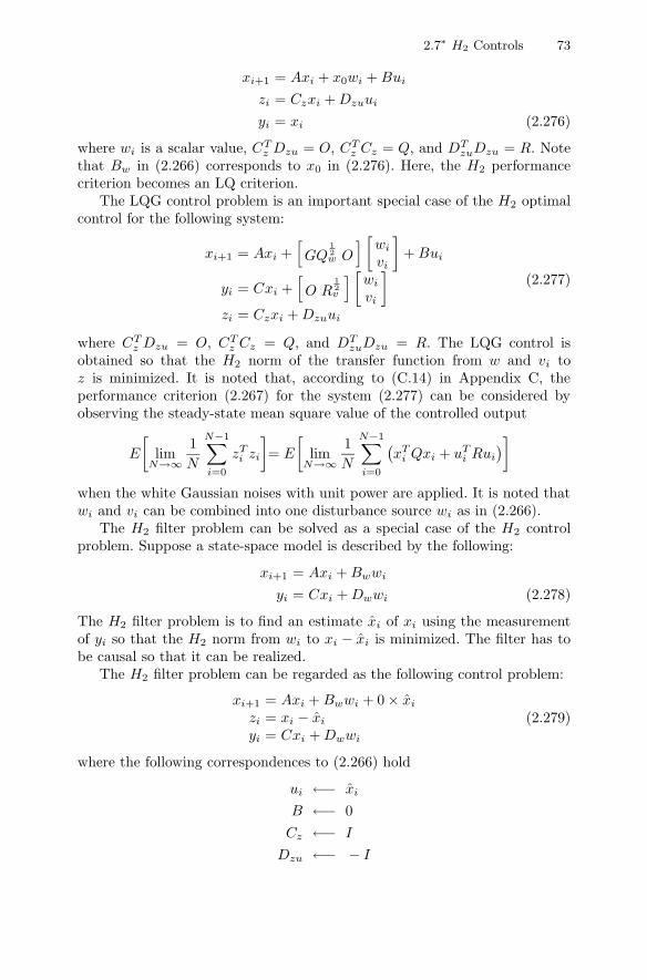
2.7∗ H2 Controls 73

xi+1 = Axi + x0wi + Bui

zi = Czxi + Dzuui

yi = xi (2.276)

where wi is a scalar value, CTz Dzu = O, CT

z Cz = Q, and DTzuDzu = R. Note

that Bw in (2.266) corresponds to x0 in (2.276). Here, the H2 performancecriterion becomes an LQ criterion.

The LQG control problem is an important special case of the H2 optimalcontrol for the following system:

xi+1 = Axi +[GQ

12w O

] [wi

vi

]+ Bui

yi = Cxi +[O R

12v

] [wi

vi

]zi = Czxi + Dzuui

(2.277)

where CTz Dzu = O, CT

z Cz = Q, and DTzuDzu = R. The LQG control is

obtained so that the H2 norm of the transfer function from w and vi toz is minimized. It is noted that, according to (C.14) in Appendix C, theperformance criterion (2.267) for the system (2.277) can be considered byobserving the steady-state mean square value of the controlled output

E

[lim

N→∞1N

N−1∑i=0

zTi zi

]= E

[lim

N→∞1N

N−1∑i=0

(xT

i Qxi + uTi Rui

)]when the white Gaussian noises with unit power are applied. It is noted thatwi and vi can be combined into one disturbance source wi as in (2.266).

The H2 filter problem can be solved as a special case of the H2 controlproblem. Suppose a state-space model is described by the following:

xi+1 = Axi + Bwwi

yi = Cxi + Dwwi (2.278)

The H2 filter problem is to find an estimate xi of xi using the measurementof yi so that the H2 norm from wi to xi − xi is minimized. The filter has tobe causal so that it can be realized.

The H2 filter problem can be regarded as the following control problem:

xi+1 = Axi + Bwwi + 0 × xi

zi = xi − xi

yi = Cxi + Dwwi

(2.279)

where the following correspondences to (2.266) hold

ui ←− xi

B ←− 0Cz ←− I

Dzu ←− − I

74 2 Optimal Controls on Finite and Infinite Horizons: A Review

H2/H∞ Controls Based on Mixed Criteria

Each performance criterion has its own advantages and disadvantages, so thatthere are trade-offs between them. In some cases we want to adopt two or moreperformance criteria simultaneously in order to satisfy specifications. In thissection, we introduce two kinds of controls based on mixed criteria. It is notedthat an LQ control is a special case of H2 controls. Here, the LQ control isused for simplicity.

1. Minimize the H2 norm for a fixed guaranteed H∞ norm such that

minγ2,Y,S

γ2 (2.280)

subject to

[γ2 xT

0

x0 S

]≥ 0 (2.281)⎡⎢⎢⎣

−S (AS + BY )T Y T S(AS + BY ) −S 0 0

Y 0 −R−1 0S 0 0 −Q−1

⎤⎥⎥⎦ ≤ 0 (2.282)

⎡⎢⎢⎣−S (AS + BY ) Bw 0

(AS + BY )T −S 0 (CzS + DzuY )T

BTw 0 −γ∞I 00 (CzS + DzuY ) 0 −γ∞I

⎤⎥⎥⎦ < 0 (2.283)

From Y and S, the state feedback gain is obtained, i.e. H = Y S−1.2. Minimize the H∞ norm for a fixed guaranteed H2 norm such that

minγ∞,Y,S

γ∞ (2.284)

subject to(2.281), (2.282), (2.283).

The state feedback gain is obtained from Y and S, i.e. H = Y S−1.

2.8 References

The material presented in this chapter has been established for a long timeand is covered in several excellent books. The subject is so large that it wouldbe a considerable task to provide comprehensive references.

Therefore, in this chapter, some references will be provided so that it isenough to understand the contents.

2.8 References 75

Dynamic programming and the minimum principle of Section 2.2 are dis-cussed in many places. For general systems, dynamic programming and theminimum principle of Pontryagin appeare in [BD62, BK65, Bel57] and in[PBGM62] respectively. For a short review, [Kir70] is a useful reference forthe minimum criterion in both dynamic programming and the minimum prin-ciple. For a treatment of the minimax criterion, see [Bur98] for the minimaxprinciple and [BB91] [BLW91] [KIF93] for dynamic programming. Readersinterested in rigorous mathematics are referred to [Str68].

The literature on LQ controls is vast and old. LQR for tracking problemsas in Theorems 2.1, 2.2, and 2.4 is via dynamic programming [AM89] and viathe minimum principle [BH75] [KS72]. In the case of a fixed terminal with areference signal, the closed-loop solution is first introduced in this book as inTheorem 2.3.

The H∞ control in Section 2.3.2 is closely related to an LQ differencegame. The books by [BH75] and [BO82] are good sources for results on gametheories. [BB91] is a book on game theories that deals explicitly with theconnections between game theories and H∞ control. The treatment of thefinite horizon state feedback H∞ control in this book is based on [LAKG92].

The Kalman filters as in Theorem 2.6 can be derived in many ways forstochastic systems. The seminal papers on the optimal estimation are [KB60]and [KB61].

The perfect square expression of the quadratic cost function in Lemmas2.8 and 2.9 appeared in [Lew86b, Lew86a]. A bibliography of LQG controls iscompiled by [MG71]. A special issue of the IEEE Transactions on AutomaticControl was devoted to LQG controls in 1971 [Ath71]. Most of the contentsabout LQG in this book originate from the text of [Lew86b]. The LQG sep-aration theorem appeared in [Won68]. The perfect square expression of theH∞ cost function in Theorem 2.11 appeared in [GL95].

Even though finite horizon and infinite horizon LQ controls are obtainedanalytically from a Riccati approach, we also obtain them numerically froman LMI in this book, which can be useful for constrained systems. Detailedtreatments of LMI can be found in [BGFB94, GNLC95]. The LMIs for LQ andH∞ controls in Sections 2.6.1 and 2.6.2 appear in [GNLC95]. The boundedreal lemma in Section 2.6.2 is investigated in [Yak62], [Kal63], and [Pop64],and also in a book by [Bur98].

The general H2 problem and its solution are considered well in the fre-quency domain in [ZDG96]. This work is based on the infinite horizon. In[BGFB94], H2 and H∞ controls are given in LMI form, which can be usedfor the H2/H∞ mixed control. The work by [BH89] deals with the problemrequiring the minimization of an upper bound on the H2 norm under an H∞norm constraint.

76 2 Optimal Controls on Finite and Infinite Horizons: A Review

2.9 Problems

2.1. Consider the system

xi+1 = αxi + ui −u2

i

M − xi(2.285)

where 0 < α < 1 and xi0 < M . In particular, we want to maximize

J = βif−i0cxif+

if−1∑i=i0

[pxi − ui]βi−i0 (2.286)

where p > 0, 0 < β < 1, and c > 0. Find an optimal control ui so that (2.286)is maximized.

2.2. Consider a nonlinear system xk+1 = f(xk, uk) with constraints given byφ(xk) ≥ 0 and the performance criterion (2.2).

(1) Show that above φ(xk) ≥ 0 can be represented by an extra state variablexn+1,k+1 such as

xn+1,k+1 = xn+1,k + [φ1(xk)]2u(−φ1(xk)) + · · · + [φl(xk)]2u(−φl(xk))

where u(·) is a unit function given by u(x) = 1 only for x > 0 and 0otherwise with

xn+1,i0 = 0, xn+1,if= 0

(2) Using the minimum principle, find the optimal control so that the system

x1,k+1 = 0.4x2,k (2.287)x2,k+1 = −0.2x2,k + uk (2.288)

is to be controlled to minimize the performance criterion

J =3∑

k=0

0.5[x21,k + x2

2,k + u2k] (2.289)

The control and states are constrained by

−1 ≤ uk ≤ 1 (2.290)−2 ≤ x2,k ≤ 2 (2.291)

2.3. Suppose that a man has his initial savings S and lives only on interestthat comes from his savings at a fixed rate. His current savings xk are thereforegoverned by the equation

xk+1 = αxk − uk (2.292)

2.9 Problems 77

where α > 1 and uk denotes his expenditure. His immediate enjoyment dueto expenditure is uk

12 . As time goes on, the enjoyment is diminished as fast

as βk, where |β| < 1. Thus, he wants to maximize

J =N∑

k=0

βku12k (2.293)

where S, α, and β are set to 10, 1.8, and 0.6, respectively. Make simulationsfor three kinds of planning based on Table 1.1. For the long-term planning,use N = 100. For the periodic and short-term plannings, use N = 5 and thesimulation time is 100. Using the minimum principle, find optimal solutionsui analytically, not numerically.

2.4. Consider the following general nonlinear system:

xi+1 = f(xi) + g(xi)wi, zi = h(xi) + J(xi)wi (2.294)

(1) If there exists a nonnegative function V : n → with V (0) = 0 suchthat for all w ∈ p and k = 0, 1, 2 · · ·

V (xk+1) − V (xk) ≤ γ2‖wk‖2 − ‖zk‖2 (2.295)

show that the following inequality is satisfied:

N∑k=0

||zk||2 ≤ γ2N∑

k=0

||wk||2

Conversely, show that a nonnegative function V : n → with V (0) = 0exists if the H∞ norm of the system is less than γ2.(2) Suppose that there exists a positive definite function V (x) satisfying

gT (0)∂2V

∂2x(0)g(0) + JT (0)J(0) − γ2 < 0 (2.296)

0 = V (f(x) + g(x)α(x)) − V (x)

+12(||h(x) + J(x)α(x)|| − γ2||α(x)||) (2.297)

where α(x) is a unique solution of

∂V

∂α(x)(x)g(x) + α(x)T (JT (x)J(x) − γ2) = −hT (x)J(x) (2.298)

and the systems is observable, i.e.

zk|wk=0 = h(xk) = 0 → limk→∞

xk = 0 (2.299)

Show that the system xi+1 = f(xi) is stable.

78 2 Optimal Controls on Finite and Infinite Horizons: A Review

2.5. We consider a minimum time performance criterion in which the objectiveis to steer a current state into a specific target set in minimum time.

For the system

xi+1 =[

1 10 1

]xi +

[0.51

]ui (2.300)

the performance criterion is given as

J =if−1∑i=i0

1 = if − i0 (2.301)

where |ui| ≤ 1. Find the control ui to bring the state from the initial pointxi0 = [1 4]T to the origin in the minimum time.

2.6. An optimal investment plan is considered here. Without any externalinvestment, the manufacturing facilities at the next time k + 1 decrease inproportion to the manufacturing facilities at the current time k. In order toincrease the manufacturing facilities, we should invest money. Letting xk anduk be the manufacturing facilities at time k and the investment at the time krespectively, we can construct the following model:

xk+1 = αxk + γuk (2.302)

where |α| < 1, γ > 0, and x0 are given. Assume that manufacturing facilitiesare worth the value proportional to the investment and the product at thetime k is proportional to the manufacturing facilities at time k. Then, theprofit can be represented as

J = βxN +N−1∑i=0

(βxi − ui) (2.303)

The investment is assumed to be nonnegative and bounded above, i.e. 0 ≤ui ≤ u. Obtain the optimal investment with respect to α, β, γ, and N .

2.7. Let a free body obey the following dynamics:

yi+1 = yi + vi (2.304)vi+1 = vi + ui (2.305)

with yi the position and vi the velocity. The state is xi = [yi vi]T . Let theacceleration input ui be constrained in magnitude by

|ui| ≤ 1 (2.306)

Suppose the objective is to determine a control input to bring any given initialstate (yi0 , vi0) to the origin so that

2.9 Problems 79[yif

vif

]= 0 (2.307)

The control should use minimum fuel, so let

J(i0) =if∑

i=i0

|ui| (2.308)

(1) Find the minimum-fuel control law to drive any xi0 to the origin in a giventime N = if − i0 if |ui| ≤ 1.(2) Draw the phase-plane trajectory. N , yi0 , and vi0 are set to 35, 10, and 10respectively.

2.8. Consider a performance criterion with Q = R = 0 and a positive definiteQf . The control can be given (2.43)–(2.45) with the inverse replaced by apseudo inverse.

(1) Show that the solution to Riccati Equation (3.47) can be represented as

Kif−k = (Q12f Ak)T

[I − Q

12f Wk(Q

12f Wk)T [Q

12f Wk(Q

12f Wk)T ]†

](Q

12f Ak). (2.309)

where Wk = [B AB A2B · · · Ak−1B] for k = 1, 2, ..., N−1 with W0 = 0and A† is a pseudo inverse of A.

(2) In the deadbeat control problem, we desire that xif= 0; this can happen

only if a performance criterion is equal to zero, i.e. if Ki0 = 0. Show thatKi0 can be zero if the following condition holds for some k:

Im(Ak) ⊂ Im(Wk) (2.310)

where Im(M) is the image of the matrix M .(3) Show that (2.310) is satisfied if the system is controllable.

2.9. Consider the following performance criterion for the system (2.27):

J(xr, u) =if−1∑i=i0

[xi

ui

]T [Q M

MT R

] [xi

ui

]+ xT

ifQfxif

where

Q = QT ≥ 0,[

Q MMT R

]≥ 0, R = RT > 0

Show that the optimal control is given as

ui = −Kixi

Ki = (BT Si+1B + R)−1(BT Si+1A + MT )Si = AT Si+1A − (BT Si+1A + MT )T (BT Si+1B + R)−T (BT Si+1A + MT )

+ Q

where Sif= Qf .

80 2 Optimal Controls on Finite and Infinite Horizons: A Review

2.10. Show that the general tracking control (2.103) is reduced to the simplertracking control (2.79) if Q in (2.103) becomes zero.

2.11. Consider the minimum energy performance criterion given by

J =if−1∑i=i0

uTi Rui (2.311)

for the system (2.27). Find the control ui that minimizes (2.311) and satisfiesthe constraints |ui| ≤ u and xif

= 0.

2.12. Consider an optimal control problem on [i0 if ] for the system (2.27)with the LQ performance criterion

J(x, u) =if−1∑i=i0

(xTi Qxi + uT

i Rui) (2.312)

(1) Find the optimal control uk subject to Cxif+ b = 0.

(2) Find the optimal control uk subject to xTif

Pxif≤ 1, where P is a sym-

metric positive definite matrix.

2.13. Consider the following performance criterion for the system (2.120):

J(xr, u) =if−1∑i=i0

[xi

ui

]T [Q M

MT R

] [xi

ui

]− γ2wT

i wi

+xT

ifQfxif

,

where

Q = QT ≥ 0,[

Q MMT R

]≥ 0, R = RT > 0. (2.313)

Derive the H∞ control.

2.14. Derive the last term hi,ifin the optimal cost (2.148) associated with

the H∞ control.

2.15. Consider the stochastic model (2.161) and (2.162) where wi and vi arezero-mean, white noise sequences with variance given by

E[

wi

vi

] [wT

j vTj

]=[

Ξ11 Ξ12

Ξ12 Ξ22

]δi−j

(1) Show that (2.161) and (2.162) are equivalent to the following model:

xi+1 = Axi + Bui + GΞ12Ξ−122 yi + Gξi

yi = Cxi + vi

where

A = A − GΞ12Ξ−122 C, ξi = wi − Ξ12Ξ

−122 vi

2.9 Problems 81

(2) Find EξivTi .

(3) Show that the controllability and observability of the pairs A, B andA, C are guaranteed by the controllability and observability of the pairsA,B and A,C, respectively.

(4) Find the Kalman filter xk+1|k.

2.16. Consider the following system:

xk+1 =

⎡⎣0 1 00 0 10 0 0

⎤⎦xk +

⎡⎣001

⎤⎦ ξk

yk =[1 0 0

]xk + θk

where ξk and θk are zero-mean Gaussian white noises with covariance 1 andµ.

(1) Express the covariance of the state estimation error Pk as a function of µ.(2) Calculate the gain matrix of the Kalman filter.(3) Calculate and plot the poles and zeros of the closed-loop system.

2.17. Consider the LQG problem[x1,i+1

x2,i+1

]=[

1 10 1

] [x1,i

x2,i

]+

√ρ

[1 01 0

]w +

[01

]u (2.314)

y =[1 0] [x1

x2

](2.315)

for the following performance criterion:

J =if−1∑i=i0

ρ(x1 + x2)2 + u2i (2.316)

Discuss the stability margin, such as gain and phase margins, for steady-statecontrol.

2.18. Consider a controllable pair A,B and assume A does not have unit-circle eigenvalues. Consider also arbitrary matrices Q,S,R of appropriatedimensions and define a Popov function

Sy(z) =[BT (zI − AT )−1 I

] [ Q SST R

] [(z−1I − A)−1B

I

](2.317)

where the central matrix is Hermitian but may be indefinite. The KYPlemma[KSH00] can be stated as follows.The following three statements are all equivalent:

(a) Sy(ejw) ≥ 0 for all w ∈ [−π , π].

82 2 Optimal Controls on Finite and Infinite Horizons: A Review

(b) There exists a Hermitian matrix P such that[Q − P + AT PA S + AT PB

ST + BT PA R + BT PB

]≥ 0 (2.318)

(c) There exist an n × n Hermitian matrix P , a p × p matrix Re ≥ 0, and ann × p matrix Kp, such that[

Q − P + AT PA S + AT PBST + BT PA R + BT PB

]=[

Kp

I

]Re

[KT

p I]

(2.319)

Derive the bounded real lemma from the above KYP lemma and compare itwith the LMI result in this section.

3

State Feedback Receding Horizon Controls

3.1 Introduction

In this chapter, state feedback receding horizon controls for linear systemswill be given for both quadratic and H∞ performance criteria.

The state feedback receding horizon LQ controls will be extensively inves-tigated because they are bases for the further developments of other recedingcontrols. The receding horizon control with the quadratic performance cri-terion will be derived with detailed procedures. Time-invariant systems aredealt with with simple notations. The important monotonicity of the opti-mal cost will be introduced with different conditions, such as a free terminalstate and a fixed terminal state. A nonzero terminal cost for the free terminalstate is often termed a free terminal state thereafter, and a fixed terminalstate as a terminal equality constraint thereafter. Stability of the recedinghorizon controls is proved under cost monotonicity conditions. Horizon sizesfor guaranteeing the stability are determined regardless of terminal weight-ing matrices. Some additional properties of the receding horizon controls arepresented.

Similar results are given for the H∞ controls that are obtained from theminimax criterion. In particular, monotonicity of the saddle-point value andstability of the state feedback receding horizon H∞ controls are discussed.

Since cost monotonicity conditions look difficult to obtain, we introduceeasy computation of receding horizon LQ and H∞ controls by the LMI.

In order to explain the concept of a receding horizon, we introduce the pre-dictive form, say xk+j , and the referenced predictive form, say xk+j|k, in thischapter. Once the concept is clearly understood by using the reference predic-tive form, we will use the predictive form instead of the reference predictiveform.

The organization of this chapter is as follows. In Section 3.2, predictiveforms for systems and performance criteria are introduced. In Section 3.3, re-ceding horizon LQ controls are extensively introduced with cost monotonicity,stability, and internal properties. A special case of input–output systems is

84 3 State Feedback Receding Horizon Controls

investigated for GPC. In Section 3.4, receding horizon H∞ controls are dealtwith with cost monotonicity, stability, and internal properties. In Section 3.5,receding horizon LQ control and H∞ control are represented via batch andLMI forms.

3.2 Receding Horizon Controls in Predictive Forms

3.2.1 Predictive Forms

Consider the following state-space model:

xi+1 = Axi + Bui (3.1)zi = Czxi (3.2)

where xi ∈ n and ui ∈ m are the state and the input respectively. zi in(3.2) is called a controlled output. Note that the time index i is an arbitrarytime point. This time variable will also be used for recursive equations.

With the standard form (3.1) and (3.2) it is not easy to represent thefuture time from the current time. In order to represent the future time fromthe current time, we can introduce a predictive form

xk+j+1 = Axk+j + Buk+j (3.3)zk+j = Czxk+j (3.4)

where k and j indicate the current time and the time distance from it re-spectively. Note that xk+j , zk+j , and uk+j mean future state, future output,and future input at time k + j respectively. In the previous chapter it wasnot necessary to identify the current time. However, in the case of the RHCthe current time and the specific time points on the horizon should be dis-tinguished. Thus, k is used instead of i for RHC, which offers a clarificationduring the derivation procedure. The time on the horizon denoted by k + jmeans the time after j from the current time. This notation is depicted inFigure 3.1. However, the above predictive form also does not distinguish thecurrent time if they are given as numbers. For example, k = 10 and j = 3give xk+j = x13. When x13 is given, there is no way to know what the currenttime is. Therefore, in order to identify the current time we can introduce areferenced predictive form

xk+j+1|k = Axk+j|k + Buk+j|k (3.5)zk+j|k = Czxk+j|k (3.6)

with the initial condition xk|k = xk. In this case, when k = 10 and j = 3,xk+j|k can be represented as x13|10. We can see that the current time k is 10and the distance j from the current time is 3. A referenced predictive form

3.2 Receding Horizon Controls in Predictive Forms 85

Fig. 3.1. Times in predictive forms

improves understanding. However, a predictive form will often be used in thisbook because the symbol k indicates the current time.

For a minimax problem, the following system is considered:

xi+1 = Axi + Bui + Bwwi (3.7)zi = Czxi (3.8)

where wi is a disturbance. In order to represent the future time we can intro-duce a predictive form

xk+j+1 = Axk+j + Buk+j + Bwwk+j (3.9)zk+j = Czxk+j (3.10)

and a referenced predictive form

xk+j+1|k = Axk+j|k + Buk+j|k + Bwwk+j (3.11)zk+j|k = Czxk+j|k (3.12)

with the initial condition xk|k = xk.In order to explain the concept of a receding horizon, we introduce the

predictive form and the referenced predictive form. Once the concept is clearlyunderstood by using the referenced predictive form, we will use the predictiveform instead of the referenced predictive form for notational simplicity.

3.2.2 Performance Criteria in Predictive Forms

In the minimum performance criterion (2.31) for the free terminal cost, i0 canbe arbitrary and is set to k so that we have

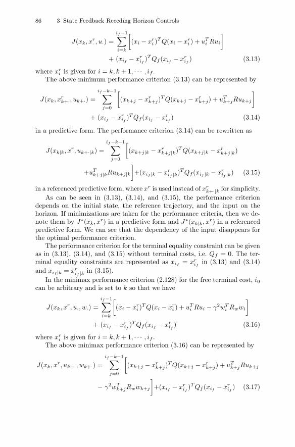
86 3 State Feedback Receding Horizon Controls

J(xk, xr· , u·) =

if−1∑i=k

[(xi − xr

i )T Q(xi − xr

i ) + uTi Rui

]+ (xif

− xrif

)T Qf (xif− xr

if) (3.13)

where xri is given for i = k, k + 1, · · · , if .

The above minimum performance criterion (3.13) can be represented by

J(xk, xrk+·, uk+·) =

if−k−1∑j=0

[(xk+j − xr

k+j)T Q(xk+j − xr

k+j) + uTk+jRuk+j

]+ (xif

− xrif

)T Qf (xif− xr

if) (3.14)

in a predictive form. The performance criterion (3.14) can be rewritten as

J(xk|k, xr, uk+·|k) =if−k−1∑

j=0

[(xk+j|k − xr

k+j|k)T Q(xk+j|k − xrk+j|k)

+uTk+j|kRuk+j|k

]+(xif |k − xr

if |k)T Qf (xif |k − xrif |k) (3.15)

in a referenced predictive form, where xr is used instead of xrk+·|k for simplicity.

As can be seen in (3.13), (3.14), and (3.15), the performance criteriondepends on the initial state, the reference trajectory, and the input on thehorizon. If minimizations are taken for the performance criteria, then we de-note them by J∗(xk, xr) in a predictive form and J∗(xk|k, xr) in a referencedpredictive form. We can see that the dependency of the input disappears forthe optimal performance criterion.

The performance criterion for the terminal equality constraint can be givenas in (3.13), (3.14), and (3.15) without terminal costs, i.e. Qf = 0. The ter-minal equality constraints are represented as xif

= xrif

in (3.13) and (3.14)and xif |k = xr

if |k in (3.15).In the minimax performance criterion (2.128) for the free terminal cost, i0

can be arbitrary and is set to k so that we have

J(xk, xr, u·, w·) =if−1∑i=k

[(xi − xr

i )T Q(xi − xr

i ) + uTi Rui − γ2wT

i Rwwi

]+ (xif

− xrif

)T Qf (xif− xr

if) (3.16)

where xri is given for i = k, k + 1, · · · , if .

The above minimax performance criterion (3.16) can be represented by

J(xk, xr, uk+·, wk+·) =if−k−1∑

j=0

[(xk+j − xr

k+j)T Q(xk+j − xr

k+j) + uTk+jRuk+j

− γ2wTk+jRwwk+j

]+(xif

− xrif

)T Qf (xif− xr

if) (3.17)

3.3 Receding Horizon Control Based on Minimum Criteria 87

in a predictive form. The performance criterion (3.17) can be rewritten as

J(xk|k, xr, uk+·|k, wk+·|k) =if−k−1∑

j=0

[(xk+j|k − xr

k+j|k)T Q(xk+j|k − xrk+j|k)

+ uTk+j|kRuk+j|k − γ2wT

k+j|kRwwk+j|k

]+ (xif |k − xr

if |k)T Qf (xif |k − xrif |k) (3.18)

in a referenced predictive form.Unlike the minimization problem, the performance criterion for the min-

imaxization problem depends on the disturbance. Taking the minimizationand the maximization with respect to the input and the disturbance respec-tively yields the optimal performance criterion that depends only on the ini-tial state and the reference trajectory. As in the minimization problem, wedenote the optimal performance criterion by J∗(xk, xr) in a predictive formand J∗(xk|k, xr) in a referenced predictive form.

3.3 Receding Horizon Control Based on MinimumCriteria

3.3.1 Receding Horizon Linear Quadratic Control

Consider the following discrete time-invariant system of a referenced predictiveform:

xk+j+1|k = Axk+j|k + Buk+j|k (3.19)zk+j|k = Czxk+j|k (3.20)

A state feedback RHC for the system (3.19) and (3.20) is introduced in atracking form. As mentioned before, the current time and the time distancefrom the current time are denoted by k and j for clarification. The time vari-able j is used for the derivation of the RHC.

Free Terminal Cost

The optimal control for the system (3.19) and (3.20) and the free terminalcost (3.18) can be rewritten in a referenced predictive form as

u∗k+j|k = −R−1BT [I + Kk+j+1,if |kBR−1BT ]−1

× [Kk+j+1,if |kAxk+j|k + gk+j+1,if |k] (3.21)

where

88 3 State Feedback Receding Horizon Controls

Kk+j,if |k = AT [I + Kk+j+1,if |kBR−1BT ]−1Kk+j+1,if |kA + Q

gk+j,if |k = AT [I + Kk+j+1,if |kBR−1BT ]−1gk+j+1,if |k − Qxrk+j|k

with Kif ,if |k = Qf and gif ,if |k = −Qfxrif |k.

The receding horizon concept was introduced in the introduction chapterand is depicted in Figure 3.2. The optimal control is obtained first on thehorizon [k, k + N ]. Here, k indicates the current time and k + N , is the finaltime on the horizon. Therefore, if = k + N , where N is the horizon size. The

Fig. 3.2. Concept of receding horizon

performance criterion can be given in a referenced predictive form as

J(xk|k, xr, uk+·|k) =N−1∑j=0

[(xk+j|k − xr

k+j|k)T Q(xk+j|k − xrk+j|k)

+uTk+j|kRuk+j|k

]+(xk+N |k − xr

k+N |k)T Qf (xk+N |k − xrk+N |k) (3.22)

The optimal control on the interval [k, k+N ] is given in a referenced predictiveform by

u∗k+j|k = −R−1BT [I + Kk+j+1,k+N |kBR−1BT ]−1

× [Kk+j+1,k+N |kAxk+j|k + gk+j+1,k+N |k] (3.23)

3.3 Receding Horizon Control Based on Minimum Criteria 89

where Kk+j+1,k+N |k and gk+j+1,k+N |k are given by

Kk+j,k+N |k = AT [I + Kk+j+1,k+N |kBR−1BT ]−1Kk+j+1,k+N |kA

+ Q (3.24)gk+j,k+N |k = AT [I + Kk+j+1,k+N |kBR−1BT ]−1gk+j+1,k+N |k

− Qxrk+j|k (3.25)

with

Kk+N,k+N |k = Qf (3.26)gk+N,k+N |k = −Qfxr

k+N |k (3.27)

The receding horizon LQ control at time k is given by the first control uk|kamong uk+i|k for i = 0, 1, · · · , k + N − 1 as in Figure 3.2. It can be obtainedfrom (3.23) with j = 0 as

u∗k|k = −R−1BT [I + Kk+1,k+N |kBR−1BT ]−1

× [Kk+1,k+N |kAxk + gk+1,k+N |k] (3.28)

where Kk+1,k+N |k and gk+1,k+N |k are computed from (3.24) and (3.25).The above notation in a referenced predictive form can be simplified to a

predictive form by dropping the reference value.It simply can be represented by a predictive form

u∗k+j = −R−1BT [I + Kk+j+1,if

BR−1BT ]−1

× [Kk+j+1,ifAxk+j + gk+j+1,if

] (3.29)

where

Kk+j,if= AT [I + Kk+j+1,if

BR−1BT ]−1Kk+j+1,ifA + Q (3.30)

gk+j,if= AT [I + Kk+j+1,if

BR−1BT ]−1gk+j+1,if− Qxr

k+j (3.31)

with Kif ,if= Qf and gif ,if

= −Qfxrif

. Thus, uk|k and Kk+1,k+N |k are re-placed by uk and Kk+1,k+N so that we have

u∗k = −R−1BT [I + Kk+1,k+NBR−1BT ]−1[Kk+1,k+NAxk + gk+1,k+N ] (3.32)

where Kk+1,k+N and gk+1,k+N are computed from

Kk+j,k+N = AT [I + Kk+j+1,k+NBR−1BT ]−1Kk+j+1,k+NA + Q (3.33)gk+j,k+N = AT [I + Kk+j+1,k+NBR−1BT ]−1gk+j+1,k+N − Qxr

k+j (3.34)

with

Kk+N,k+N = Qf (3.35)gk+N,k+N = −Qfxr

k+N (3.36)

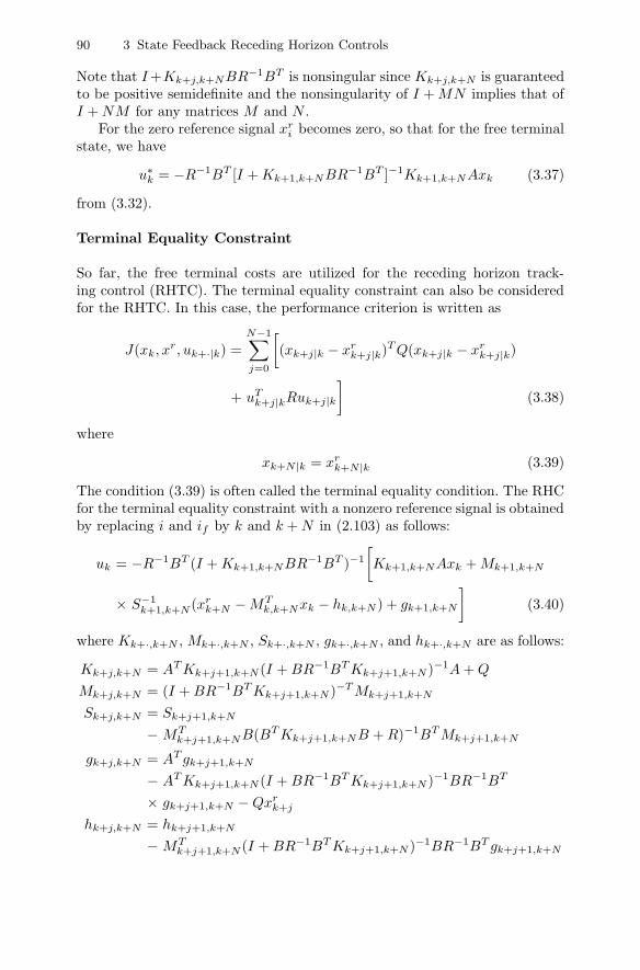
90 3 State Feedback Receding Horizon Controls

Note that I +Kk+j,k+NBR−1BT is nonsingular since Kk+j,k+N is guaranteedto be positive semidefinite and the nonsingularity of I + MN implies that ofI + NM for any matrices M and N .

For the zero reference signal xri becomes zero, so that for the free terminal

state, we have

u∗k = −R−1BT [I + Kk+1,k+NBR−1BT ]−1Kk+1,k+NAxk (3.37)

from (3.32).

Terminal Equality Constraint

So far, the free terminal costs are utilized for the receding horizon track-ing control (RHTC). The terminal equality constraint can also be consideredfor the RHTC. In this case, the performance criterion is written as

J(xk, xr, uk+·|k) =N−1∑j=0

[(xk+j|k − xr

k+j|k)T Q(xk+j|k − xrk+j|k)

+ uTk+j|kRuk+j|k

](3.38)

where

xk+N |k = xrk+N |k (3.39)

The condition (3.39) is often called the terminal equality condition. The RHCfor the terminal equality constraint with a nonzero reference signal is obtainedby replacing i and if by k and k + N in (2.103) as follows:

uk = −R−1BT (I + Kk+1,k+NBR−1BT )−1

[Kk+1,k+NAxk + Mk+1,k+N

× S−1k+1,k+N (xr

k+N − MTk,k+Nxk − hk,k+N ) + gk+1,k+N

](3.40)

where Kk+·,k+N , Mk+·,k+N , Sk+·,k+N , gk+·,k+N , and hk+·,k+N are as follows:

Kk+j,k+N = AT Kk+j+1,k+N (I + BR−1BT Kk+j+1,k+N )−1A + Q

Mk+j,k+N = (I + BR−1BT Kk+j+1,k+N )−T Mk+j+1,k+N

Sk+j,k+N = Sk+j+1,k+N

− MTk+j+1,k+NB(BT Kk+j+1,k+NB + R)−1BT Mk+j+1,k+N

gk+j,k+N = AT gk+j+1,k+N

− AT Kk+j+1,k+N (I + BR−1BT Kk+j+1,k+N )−1BR−1BT

× gk+j+1,k+N − Qxrk+j

hk+j,k+N = hk+j+1,k+N

− MTk+j+1,k+N (I + BR−1BT Kk+j+1,k+N )−1BR−1BT gk+j+1,k+N

3.3 Receding Horizon Control Based on Minimum Criteria 91

The boundary conditions are given by

Kk+N,k+N = 0,Mk+N,k+N = I, Sk+N,k+N = 0, gk+N,k+N = 0, hk+N,k+N = 0

For the regulation problem, (3.40) is reduced to

u∗k = −R−1BT (I + Kk+1,k+NBR−1BT )−1

[Kk+1,k+NA

− Mk+1,k+NS−1k+1,k+NMT

k,k+N

]xk (3.41)

From (2.68), u∗k in (3.41) is represented in another form

u∗k = −R−1BT P−1

k+1,k+N+1Axk (3.42)

where Pk+1,k+N+1 is computed from (2.65)

Pk+j,k+N+1 = A−1[I + Pk+j+1,k+N+1A

−T QA−1]−1

Pk+j+1,k+N+1A

+ BR−1BT (3.43)

with

Pk+N+1,k+N+1 = 0 (3.44)

Note that the system matrix A should be nonsingular in Riccati Equation(3.43). However, this requirement can be relaxed in the form of (3.41) or withthe batch form, which is left as a problem at the end of this chapter.

3.3.2 Simple Notation for Time-invariant Systems

In previous sections the Riccati equations have had two arguments, one ofwhich represents the terminal time. However, only one argument is used fortime-invariant systems in this section for simplicity. If no confusion arises,then one argument will be used for Riccati equations throughout this book,particularly for Riccati equations for time-invariant systems.

Time-invariant homogeneous systems such as xi+1 = f(xi) have a specialproperty known as shift invariance. If the initial condition is the same, thenthe solution depends on the distance from the initial time. Let xi,i0 denotethe solution at i with the initial i0, as can be seen in Figure 3.3. That is

xi,i0 = xi+N,i0+N (3.45)

for any N with xi0,i0 = xi0+N,i0+N .

Free Terminal Cost

Since (3.33) is also a time-invariant system, the following equation is satisfied:

Kk+j,k+N = Kj,N (3.46)

92 3 State Feedback Receding Horizon Controls

Time

Fig. 3.3. Property of shift invariance

with KN,N = Kk+N,k+N = Qf .Since N is fixed, we denote Kj,N by simply Kj and Kj satisfies the fol-

lowing equation:

Kj = AT Kj+1A − AT Ki+1B[R + BT Kj+1B]−1BT Kj+1A + Q

= AT Kj+1[I + BR−1BT Kj+1]−1A + Q (3.47)

with the boundary condition

KN = Qf (3.48)

Thus, the receding horizon control (3.32) can be represented as

u∗k = −R−1BT [I + K1BR−1BT ]−1[K1Axk + gk+1,k+N ] (3.49)

where K1 is obtained from (3.47) and gk+1,k+N is computed from

gk+j,k+N = AT [I + Kj+1BR−1BT ]−1gk+j+1,k+N − Qxrk+j (3.50)

with the boundary condition

gk+N,k+N = −Qfxrk+N (3.51)

It is noted that (3.34) is not a time-invariant system due to a time-varyingsignal, xr

k+j . If xrk+j is a constant signal denoted by xr, then

gj = AT [I + Kj+1BR−1BT ]−1gj+1 − Qxr (3.52)

with the boundary condition

3.3 Receding Horizon Control Based on Minimum Criteria 93

gN = −Qf xr (3.53)

The control can be written as

uk = −R−1BT [I + K1BR−1BT ]−1(K1Axk + g1) (3.54)

It is noted that from shift invariance with a new boundary condition

KN−1 = Qf (3.55)

K1 in (3.49) and (3.54) becomes K0.For the zero reference signal xr

i becomes zero, so that for the free terminalcost we have

u∗k = −R−1BT [I + K1BR−1BT ]−1K1Axk (3.56)

from (3.32).

Terminal Equality Constraint

The RHC (3.40) for the terminal equality constraint with a nonzero refer-ence can be represented as

uk = −R−1BT [I + K1BR−1BT ]−1

[K1Axk

+ M1S−11 (xr

k+N − MT0 xk − hk,k+N ) + gk+1,k+N

](3.57)

where Kj , Mj , Sj , gk+j,k+N , and hk+j,k+N are as follows:

Kj = AT Kj+1(I + BR−1BT Kj+1)−1A + Q

Mj = (I + BR−1BT Kj+1)−T Mj+1

Sj = Sj+1 − MTj+1B(BT Kj+1B + R)−1BT Mj+1

gk+j,k+N = AT gk+j+1,k+N

− AT Kj+1(I + BR−1BT Kj+1)−1BR−1BT gk+j+1,k+N

− Qxrk+j

hk+j,k+N = hk+j+1,k+N

− MTk+j+1,k+N (I + BR−1BT Kj+1)−1BR−1BT gk+j+1,k+N

The boundary conditions are given by

KN = 0, MN = I, SN = 0, gk+N,k+N = 0, hk+N,k+N = 0

For the regulation problem, (3.57) is reduced to

u∗k = −R−1BT [I + K1BR−1BT ]−1

[K1A − M1S

−11 MT

0

]xk (3.58)

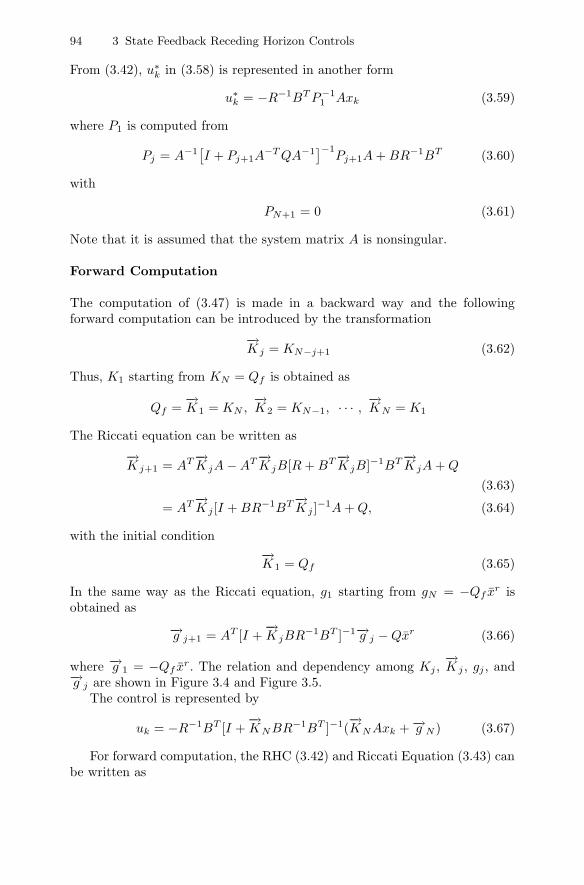
94 3 State Feedback Receding Horizon Controls

From (3.42), u∗k in (3.58) is represented in another form

u∗k = −R−1BT P−1

1 Axk (3.59)

where P1 is computed from

Pj = A−1[I + Pj+1A

−T QA−1]−1

Pj+1A + BR−1BT (3.60)

with

PN+1 = 0 (3.61)

Note that it is assumed that the system matrix A is nonsingular.

Forward Computation

The computation of (3.47) is made in a backward way and the followingforward computation can be introduced by the transformation

−→K j = KN−j+1 (3.62)

Thus, K1 starting from KN = Qf is obtained as

Qf =−→K1 = KN ,

−→K2 = KN−1, · · · ,

−→KN = K1

The Riccati equation can be written as

−→K j+1 = AT−→K jA − AT−→K jB[R + BT−→K jB]−1BT−→K jA + Q

(3.63)

= AT−→K j [I + BR−1BT−→K j ]−1A + Q, (3.64)

with the initial condition−→K1 = Qf (3.65)

In the same way as the Riccati equation, g1 starting from gN = −Qf xr isobtained as

−→g j+1 = AT [I +−→K jBR−1BT ]−1−→g j − Qxr (3.66)

where −→g 1 = −Qf xr. The relation and dependency among Kj ,−→K j , gj , and

−→g j are shown in Figure 3.4 and Figure 3.5.The control is represented by

uk = −R−1BT [I +−→KNBR−1BT ]−1(

−→KNAxk + −→g N ) (3.67)

For forward computation, the RHC (3.42) and Riccati Equation (3.43) canbe written as

3.3 Receding Horizon Control Based on Minimum Criteria 95

index

(a)

(b) (c)

(d)

Fig. 3.4. Computation of Ki and Ki. Initial conditions i = 0 in (a), i = 1 in (b),i = N − 1 in (c), and i = N in (d)

Fig. 3.5. Relation between Ki and gi

u∗k = −R−1BT−→P −1

N Axk (3.68)

where−→P N is computed by

−→P j+1 = A−1−→P j [I + A−T QA−1−→P j ]−1A−T + BR−1BT (3.69)

with−→P 1 = 0.

3.3.3 Monotonicity of the Optimal Cost

In this section, some conditions are proposed for time-invariant systems whichguarantee the monotonicity of the optimal cost. In the next section, under theproposed cost monotonicity conditions, the closed-loop stability of the RHCis shown. Since the closed-loop stability can be treated with the regulationproblem, the gi can be zero in this section.

96 3 State Feedback Receding Horizon Controls

It is noted that the cost function J (3.13)–(3.15) depends on several vari-ables, such as the initial state xi, input ui+·, initial time i, and terminal timeif . Thus, it can be represented as J(xi, ui+·, i, if ) and the optimal cost canbe given as J∗(xi, i, if ).

Define δJ∗(xτ , σ) as δJ∗(xτ , σ) = J∗(xτ , τ, σ + 1) − J∗(xτ , τ, σ). IfδJ∗(xτ , σ) ≤ 0 or δJ∗(xτ , σ) ≥ 0 for any σ > τ , then it is called a costmonotonicity. We will show first that the cost monotonicity condition can beeasily achieved by the terminal equality condition. Then, the more generalcost monotonicity condition is introduced by using a terminal cost.

For the terminal equality condition, i.e. xif= 0, we have the following

result.

Theorem 3.1. For the terminal equality constraint, the optimal cost J ∗(xi, i, if )satisfies the following cost monotonicity relation:

J∗(xτ , τ, σ + 1) ≤ J∗(xτ , τ, σ), τ ≤ σ (3.70)

If the Riccati solution exists for (3.70), then we have

Kτ,σ+1 ≤ Kτ,σ (3.71)

Proof. This can be proved by contradiction. Assume that u1i and u2

i are opti-mal controls to minimize J(xτ , τ, σ + 1) and J(xτ , τ, σ) respectively. If (3.70)does not hold, then

J∗(xτ , τ, σ + 1) > J∗(xτ , τ, σ)

Replace u1i by u2

i up to σ − 1 and then u1i = 0 at i = σ. In this case,

x1σ = 0, u1

σ = 0, and thus x1σ+1 = 0. Therefore, the cost for this control

is J(xτ , τ, σ + 1) = J∗(xτ , τ, σ). Since this control may not be optimal forJ(xτ , τ, σ + 1), we have J(xτ , τ, σ + 1) ≥ J∗(xτ , τ, σ + 1), which implies that

J∗(xτ , τ, σ) ≥ J∗(xτ , τ, σ + 1) (3.72)

This is a contradiction to (3.70). This completes the proof.

For the time-invariant systems we have

Kτ ≤ Kτ+1

The above result is for the terminal equality condition. Next, the costmonotonicity condition using a free terminal cost is introduced.

Theorem 3.2. Assume that Qf in (3.15) satisfies the following inequality:

Qf ≥ Q + HT RH + (A − BH)T Qf (A − BH) (3.73)

for some H ∈ m×n.

3.3 Receding Horizon Control Based on Minimum Criteria 97

For the free terminal cost, the optimal cost J∗(xi, i, if ) then satisfies thefollowing monotonicity relation:

J∗(xτ , τ, σ + 1) ≤ J∗(xτ , τ, σ), τ ≤ σ (3.74)

and thus

Kτ,σ+1 ≤ Kτ,σ (3.75)

Proof. u1i and u2

i are the optimal controls to minimize J(xτ , τ, σ + 1) andJ(xτ , τ, σ) respectively. If we replace u1

i by u2i up to σ − 1 and u1

σ = −Hxσ,then the cost for this control is given by

J(xτ , σ + 1)=

σ−1∑i=τ

[x2Ti Qx2

i + u2Ti Ru2

i ] + x2Tσ Qx2

σ + x2Tσ HT RHx2

σ

+ x2Tσ (A − BH)T Qf (A − BH)x2

σ

≥ J∗(xτ , σ + 1) (3.76)

where the last inequality comes from the fact that this control may not beoptimal. The difference between the adjacent optimal cost is less than or equalto zero as

J∗(xτ , σ + 1) − J∗(xτ , σ) ≤ J(xτ , σ + 1) − J∗(xτ , σ)= x2T

σ Qx2σ + x2T

σ HT RHx2σ

+ x2Tσ (A − BH)T Qf (A − BH)x2

σ − x2Tσ Qfx2

σ

= x2Tσ Q + HT RH + (A − BH)T Qf (A − BH) − Qfx2

σ

≤ 0 (3.77)

where

J∗(xτ , σ) =σ−1∑i=τ

[x2Ti Qx2

i + u2Ti Ru2

i ] + x2Tσ Qfx2

σ (3.78)

From (3.77) we have

J∗(xτ , σ) = xTτ [Kτ,σ+1 − Kτ,σ]xτ ≤ 0 (3.79)

for all xτ , and thus Kτ,σ+1 − Kτ,σ ≤ 0. This completes the proof.

It looks difficult to find out Qf and H satisfying (3.73). One approachis as follows: if H that makes A − BH Hurwitz is given, then Qf can besystematically obtained. First choose one matrix M > 0 such that M ≥ Q +HT RH. Then, calculate the solution Qf to the following Lyapunov equation:

(A − BH)T Qf (A − BH) − Qf = −M (3.80)

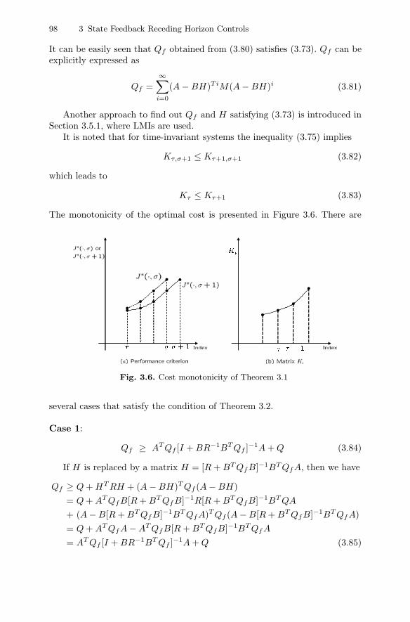
98 3 State Feedback Receding Horizon Controls

It can be easily seen that Qf obtained from (3.80) satisfies (3.73). Qf can beexplicitly expressed as

Qf =∞∑

i=0

(A − BH)TiM(A − BH)i (3.81)

Another approach to find out Qf and H satisfying (3.73) is introduced inSection 3.5.1, where LMIs are used.

It is noted that for time-invariant systems the inequality (3.75) implies

Kτ,σ+1 ≤ Kτ+1,σ+1 (3.82)

which leads to

Kτ ≤ Kτ+1 (3.83)

The monotonicity of the optimal cost is presented in Figure 3.6. There are

Fig. 3.6. Cost monotonicity of Theorem 3.1

several cases that satisfy the condition of Theorem 3.2.

Case 1:

Qf ≥ AT Qf [I + BR−1BT Qf ]−1A + Q (3.84)

If H is replaced by a matrix H = [R + BT QfB]−1BT QfA, then we have

Qf ≥ Q + HT RH + (A − BH)T Qf (A − BH)= Q + AT QfB[R + BT QfB]−1R[R + BT QfB]−1BT QA

+ (A − B[R + BT QfB]−1BT QfA)T Qf (A − B[R + BT QfB]−1BT QfA)= Q + AT QfA − AT QfB[R + BT QfB]−1BT QfA

= AT Qf [I + BR−1BT Qf ]−1A + Q (3.85)

3.3 Receding Horizon Control Based on Minimum Criteria 99

which is a special case of (3.73). All Qf values satisfying the inequality (3.85)are a subset of all Qf values satisfying (3.73).

It can be seen that (3.73) implies (3.85) regardless of H as follows:

Qf − Q − AT Qf [I + BR−1BT Qf ]−1A

≥ −AT Qf [I + BR−1BT Qf ]−1A + HT RH + (A − BH)T Qf (A − BH)

=[AT QfB(R + BT QfB)−1 − H

]T (R + BT QfB

)×[(R + BT QfB)−1BT QfA − H

]≥ 0 (3.86)

Therefore, all Qf values satisfying (3.73) also satisfy (3.85), and thus are asubset of all Qf values satisfying (3.85). Thus, (3.73) is surprisingly equivalentto (3.85).

Qf that satisfies (3.85) can also be obtained explicitly from the solutionto the following Riccati equation:

Q∗f = β2AT Q∗

f [I + γBR−1BT Q∗f ]−1A + αQ (3.87)

with α ≥ 1, β ≥ 1, and 0 ≤ γ ≤ 1. It can be easily seen that Q∗f satisfies

(3.85), since

Q∗f = β2AT Q∗

f [I + γBR−1BT Q∗f ]−1A + αQ

≥ AT Q∗f [I + BR−1BT Q∗

f ]−1A + Q

Case 2:

Qf = Q + HT RH + (A − BH)T Qf (A − BH) (3.88)

This Qf is a special case of (3.73) and has the following meaning. Notethat ui is unknown for the interval [τ σ− 1] and defined as ui = −Hxi on theinterval [σ, ∞]. If a pair (A,B) is stabilizable and ui = −Hxi is a stabilizingcontrol, then

J =∞∑

i=τ

[xTi Qxi + uT

i Rui]

=σ−1∑i=τ

[xTi Qxi + uT

i Rui]

+ xTσ

∞∑i=σ

(AT − HT BT )i−σ[Q + HT RH](A − BH)i−σxσ

=σ−1∑i=τ

[xTi Qxi + uT

i Rui] + xTσ Qfxσ (3.89)

where Qf satisfies Qf = Q + HT RH + (A − BH)T Qf (A − BH). Therefore,Qf is related to the steady-state performance with the control ui = −Hxi.

100 3 State Feedback Receding Horizon Controls

It is noted that, under (3.73), ui = −Hxi will be proved to be a stabilizingcontrol in Section 3.3.4.

Case 3:

Qf = AT Qf [I + BR−1BT Qf ]−1A + Q (3.90)

This is actually the steady-state Riccati equation and is a special case of(3.85), and thus of (3.73). This Qf is related to the steady-state optimal per-formance with the optimal control.

Case 4:

Qf = Q + AT QfA (3.91)

If the system matrix A is stable and ui is identically equal to zero fori ≥ σ ≥ τ , then Qf satisfies Qf = Q + AT QfA, which is also a special case of(3.73).

Proposition 3.3. Qf satisfying (3.73) has the following lower bound:

Qf ≥ K (3.92)

where K is the steady-state solution to the Riccati equation in (3.90) andassumed to exist uniquely.

Proof. By the cost monotonicity condition, the solution to the recursive Ric-cati equation starting from Qf satisfying Case 3 can be ordered

Qf = Ki0 ≥ Ki0+1 ≥ Ki0+2 ≥ · · · (3.93)

where

Ki+1 = AT Ki[I + BR−1BT Ki]−1A + Q (3.94)

with Ki0 = Qf .Since Ki is composed of two positive semidefinite matrices, Ki is also

positive semidefinite, or bounded below, i.e. Ki ≥ 0.Ki is decreasing and bounded below, so that Ki has a limit value, which

is denoted by K. Clearly, it can be easily seen that

Qf ≥ Ki ≥ K (3.95)

for any i ≥ i0.The only thing we have to do is to guarantee that K satisfies the condition

corresponding to Case 3. Taking the limitation on both sides of (3.94), we have

limi→∞

Ki+1 = limi→∞

AT Ki[I + BR−1BT Ki]−1A + Q (3.96)

K = AT K[I + BR−1BT K]−1A + Q (3.97)

The uniqueness of the solution to the Riccati equation implies that K is thesolution that satisfies Case 3. This completes the proof.

3.3 Receding Horizon Control Based on Minimum Criteria 101

Theorem 3.2 discusses the nonincreasing monotonicity for the optimal cost.In the following, the nondecreasing monotonicity of the optimal cost can beobtained.

Theorem 3.4. Assume that Qf in (3.15) satisfies the inequality

Qf ≤ AT Qf [I + BR−1BT Qf ]−1A + Q (3.98)

The optimal cost J∗(xi, i, if ) then satisfies the relation

J∗(xτ , τ, σ + 1) ≥ J∗(xτ , τ, σ), τ ≤ σ (3.99)

and thus

Kτ,σ+1 ≥ Kτ,σ (3.100)

Proof. u1i and u2

i are the optimal controls to minimize J(xτ , τ, σ + 1) andJ(xτ , τ, σ) respectively. If we replace u2

i by u1i up to σ−1, then by the optimal

principle we have

J∗(xτ , σ) =σ−1∑i=τ

[x2Ti Qx2

i + u2Ti Ru2

i ] + x2Tσ Qfx2

σ (3.101)

≤σ−1∑i=τ

[x1Ti Qx1

i + u1Ti Ru1

i ] + x1Tσ Qfx1

σ (3.102)

The difference between the adjacent optimal cost can be expressed as

δJ∗(xτ , σ) =σ∑

i=τ

[x1Ti Qx1

i + u1Ti Ru1

i ] + x1Tσ+1Qfx1

σ+1

−σ−1∑i=τ

[x2Ti Qx2

i + u2Ti Ru2

i ] − x2Tσ Qfx2

σ (3.103)

Combining (3.102) and (3.103) yields

δJ∗(xτ , σ) ≥ x1Tσ Qx1

σ + u1Tσ Ru1

σ + x1Tσ+1Qfx1

σ+1 − x1Tσ Qfx1

σ

= x1Tσ Q + AT Qf [I + BR−1BT Qf ]−1A − Qfx1

σ

≥ 0 (3.104)

where u1σ = −Hx1

σ, x1σ+1 = (A−BH)x1

σ and H = −(R+BT QfB)−1BT QfA.The second equality of (3.104) comes from the following fact:

HT RH + (A − BH)T Qf (A − BH) =AT Qf [I + BR−1BT Qf ]−1A (3.105)

as can be seen in (3.85). The last inequality of (3.104) comes from (3.98).From (2.49) and (3.99) we have

δJ∗(xτ , σ) = xTτ [Kτ,σ+1 − Kτ,σ]xτ ≥ 0 (3.106)

for all xτ . Thus, Kτ,σ+1 − Kτ,σ ≥ 0. This completes the proof.

102 3 State Feedback Receding Horizon Controls

It is noted that the relation (3.100) on the Riccati equation can be repre-sented simply by one argument as

Kτ ≥ Kτ+1 (3.107)

for time-invariant systems.The monotonicity of the optimal cost in Theorem 3.4 is presented in Figure

3.7.

Fig. 3.7. Cost monotonicity of Theorem 3.2

We have at least one important case that satisfies the condition of Theo-rem 3.4.

Case 1: Qf = 0

It is noted that the free terminal cost with the zero terminal weighting,Qf = 0, satisfies (3.98). Thus, Theorem 3.4 includes the monotonicity of theoptimal cost of the free terminal cost with the zero terminal weighting.

The terminal equality condition is more conservative than the free terminalcost. Actually, it is a strong requirement that the nonzero state must go to zerowithin a finite time. Thus, the terminal equality constraint has no solution forthe small horizon size N , whereas the free terminal cost always gives a solutionfor any horizon size N . The free terminal cost requires less computation thanthe terminal equality constraint. However, the terminal equality constraintprovides a simple approach for guaranteeing stability.

It is noted that the cost monotonicity in Theorems 3.1, 3.2 and 3.4 areobtained from the optimality. Thus, the cost monotonicity may hold even fornonlinear systems, which will be explained later.

In the following theorem, it will be shown that when the monotonicity ofthe optimal cost or the Riccati equations holds once, it holds for all subsequenttimes.

3.3 Receding Horizon Control Based on Minimum Criteria 103

Theorem 3.5.

(a) If

J∗(xτ ′ , τ′, σ + 1) ≤ J∗(xτ ′ , τ

′, σ) (or ≥ J∗(xτ ′ , τ

′, σ)) (3.108)

for some τ′, then

J∗(xτ ′′ , τ′′, σ + 1) ≤ J∗(xτ ′′ , τ

′′, σ) (or ≥ J∗(xτ ′′ , τ

′′, σ)) (3.109)

where τ0 ≤ τ′′ ≤ τ

′.

(b) If

Kτ ′ ,σ+1 ≤ Kτ ′ ,σ (or ≥ Kτ ′ ,σ) (3.110)

for some τ′, then

Kτ ′′ ,σ+1 ≤ Kτ ′′ ,σ (or ≥ Kτ ′′ ,σ) (3.111)

where τ0 ≤ τ′′ ≤ τ

′.

Proof. We first prove the part (a). u1i and u2

i are the optimal controls tominimize J(xτ ′′ , τ

′′, σ + 1) and J(xτ ′′ , τ

′′, σ) respectively. If we replace u1

i byu2

i up to τ ′ − 1, then by the optimal principle we have

J∗(xτ ′′ , σ + 1) =τ′−1∑

i=τ ′′[x1T

i Qx1i + u1T

i Ru1i ] + J∗(x1

τ ′ , τ′, σ + 1)

≤τ′−1∑

i=τ ′′[x2T

i Qx2i + u2T

i Ru2i ] + J∗(x2

τ ′ , τ′, σ + 1) (3.112)

The difference between the adjacent optimal cost can be expressed as

δJ∗(xτ ′′ , σ) =τ′−1∑

i=τ ′′[x1T

i Qx1i + u1T

i Ru1i ] + J∗(x1

τ ′ , τ′, σ + 1)

−τ′−1∑

i=τ ′′[x2T

i Qx2i + u2T

i Ru2i ] − J∗(x2

τ ′ , τ′, σ) (3.113)

Combining (3.112) and (3.113) yields

δJ∗(xτ ′′ , σ) ≤τ′−1∑

i=τ ′′[x2T

i Qx2i + u2T

i Ru2i ] + J∗(x2

τ ′ , τ′, σ + 1)

−τ′−1∑

i=τ ′′[x2T

i Qx2i + u2T

i Ru2i ] − J∗(x2

τ ′ , τ′, σ)

= J∗(x2τ ′ , τ

′, σ + 1) − J∗(x2

τ ′ , τ′, σ)

= δJ∗(x2τ ′ , σ) ≤ 0 (3.114)

104 3 State Feedback Receding Horizon Controls

Replacing u2i by u1

i up to τ′ − 1 and taking similar steps we have

δJ∗(xτ ′′ , σ) ≥ δJ∗(x1τ ′ , σ) (3.115)

from which δJ∗(x1τ ′ , σ) ≥ 0 implies δJ∗(xτ ′′ , σ) ≥ 0.

Now we prove the second part of the theorem. From (2.49), (3.108), and(3.109), the monotonicities of the Riccati equations hold. From the inequality

J∗(xτ ′′ , τ′′, σ + 1) − J∗(xτ ′′ , τ

′′, σ) = xT

τ ′′ [Kτ ′′ ,σ+1 − Kτ ′′ ,σ]xτ ′′

≤ (≥) 0

Kτ ′′ ,σ+1 ≤ (≥)Kτ ′′ ,σ is satisfied. This completes the proof.

For time-invariant systems the above relations can be simplified. If

Kτ ′ ≤ Kτ ′+1 (or ≥ Kτ ′+1) (3.116)

for some τ ′, then

Kτ ′′ ≤ Kτ ′′+1 (or ≥ Kτ ′′+1) (3.117)

for τ0 < τ′′

< τ′.

Part (a) of Theorem 3.5 may be extended to constrained and nonlinearsystems, whereas part (b) is only for linear systems.

Computation of the solutions of cost monotonicity conditions (3.73),(3.84), and (3.98) looks difficult to solve, but it can be easily solved by usingLMI, as seen in Section 3.5.1.

3.3.4 Stability of Receding Horizon Linear Quadratic Control

For the existence of a stabilizing feedback control, we assume that the pair(A, B) is stabilizable. In this section it will be shown that the RHC is a stablecontrol under cost monotonicity conditions.

Theorem 3.6. Assume that the pairs (A,B) and (A,Q12 ) are stabilizable and

observable respectively, and that the receding horizon control associated withthe quadratic cost J(xi, i, i+N) exists. If J∗(xi, i, i+N +1) ≤ J∗(xi, i, i+N),then asymptotical stability is guaranteed.

Proof. For time-invariant systems, the system is asymptotically stable if thezero state is attractive. We show that the zero state is attractive. SinceJ∗(xi, i, σ + 1) ≤ J∗(xi, i, σ),

J∗(xi, i, i + N) = xTi Qxi + u∗T

i Ru∗i + J∗(x(i + 1;xi, i, u

∗i ), i + 1, i + N)

≥ xTi Qxi + u∗T

i Ru∗i

+ J∗(x(i + 1;xi, i, u∗i ), i + 1, i + N + 1) (3.118)

3.3 Receding Horizon Control Based on Minimum Criteria 105

Note that ui is the receding horizon control since it is the first control on theinterval [i, i + N ]. From (3.118) we have

J∗(xi, i, i + N) ≥ J∗(x(i + 1;xi, i, u∗i ), i + 1, i + N + 1) (3.119)

Recall that a nonincreasing sequence bounded below converges to a constant.Since J∗(xi, i, i + N) is nonincreasing and J∗(xi, i, i + N) ≥ 0, we have

J∗(xi, i, i + N) → c (3.120)

for some nonnegative constant c as i → ∞. Thus, as i → ∞,

u∗Ti Ru∗

i + xTi Qxi → 0 (3.121)

andi+l−1∑j=i

xTj Qxj + u∗T

j Ru∗j = xT

i

i+l−1∑j=i

(AT − LTf BT )j−i(Q + LT

f RLf )

× (A − BLf )j−ixi = xTi Go

i,i+lxi −→ 0,

where Lf is the feedback gain of the RHC and Goi,i+l is an observability

Gramian of (A − BLf , (Q + LTf RLf )

12 ). However, since the pair (A,Q

12 ) is

observable, it is guaranteed that Goi,i+l is nonsingular for l ≥ nc by Theorem

B.5 in Appendix B. This means that xi → 0 as i → ∞, independently of i0.Therefore, the closed-loop system is asymptotically stable. This completes theproof.

Note that if the condition Q > 0 is added in the condition of Theorem 3.6,then the horizon size N could be greater than or equal to 1.

The observability in Theorem 3.6 can be weakened with the detectabilitysimilarly as in [KK00].

It was proved in the previous section that the optimal cost with the termi-nal equality constraint has a nondecreasing property. Therefore, we have thefollowing result.

Theorem 3.7. Assume that the pairs (A,B) and (A,Q12 ) are controllable and

observable respectively. The receding horizon control (3.42) obtained from theterminal equality constraint is asymptotically stable for nc ≤ N < ∞.

Proof. The controllability and nc ≤ N < ∞ are required for the existence ofthe optimal control, as seen in Figure 2.3. Then it follows from Theorem 3.1and Theorem 3.6.

Note that if the condition Q > 0 is added in the condition of Theorem 3.7,then the horizon size N could be max(nc) ≤ N < ∞.

So far, we have discussed a terminal equality constraint. For the free ter-minal cost we have a cost monotonicity condition in Theorem 3.2 for thestability.

106 3 State Feedback Receding Horizon Controls

Theorem 3.8. Assume that the pairs (A,B) and (A,Q12 ) are stabilizable and

observable respectively. For Qf ≥ 0 satisfying (3.73) for some H, the system(3.4) with the receding horizon control (3.56) is asymptotically stable for 1 ≤N < ∞.

Theorem 3.8 follows from Theorems 3.2 and 3.6. Qf in the four cases inSection 3.3.3 satisfies (3.73) and thus the condition of Theorem 3.8.

What we have talked about so far can be seen from a different perspective.The difference Riccati equation (3.47) for j = 0 can be represented as

K1 = AT K1A − AT K1B[R + BT K1B]−1BT K1A + Q (3.122)Q = Q + K1 − K0 (3.123)

Equation (3.122) no longer looks like a recursion, but rather an algebraicequation for K1. Therefore, Equation (3.122) is called the fake ARE (FARE).

The closed-loop stability of the RHC obtained from (3.122) and (3.123)requires the condition Q ≥ 0 and the detectability of the pair (A, Q

12 ). The

pair (A, Q12 ) is detectable if the pair (A,Q

12 ) is detectable and K1 − K0 ≥ 0.

The condition K1 − K0 ≥ 0 is satisfied under the terminal inequality (3.73).

The free parameter H obtained in Theorem 3.8 is combined with theperformance criterion to guarantee the stability of the closed-loop system.However, the free parameter H can be used itself as a stabilizing control gain.

Theorem 3.9. Assume that the pairs (A,B) and (A,Q12 ) are stabilizable and

observable respectively. The system (3.4) with the control ui = −Hxi is asymp-totically stable where H is obtained from the inequality (3.73).

Proof. Let

V (xi) = xTi Qfxi (3.124)

where we can show that Qf is positive definite as follows. As just said before,Qf of (3.73) satisfies the inequality (3.84). If is defined as

= Qf − AT Qf [I + BR−1BT Qf ]−1A − Q ≥ 0 (3.125)

we can consider the following Riccati equation:

Qf = AT Qf [I + BR−1BT Qf ]−1A + Q + (3.126)

The observability of (A,Q12 ) implies the observability of (A, (Q + )

12 ), so

that the unique positive solution Qf comes from (3.126). Therefore, V (xi)can be considered to be a candidate of Lyapunov functions.

Subtracting V (xi) from V (xi+1) yields

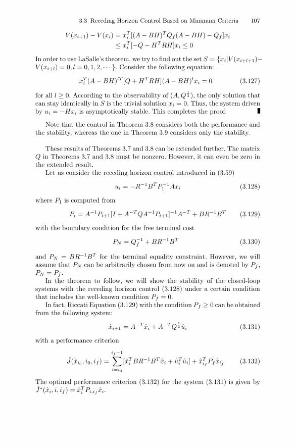
3.3 Receding Horizon Control Based on Minimum Criteria 107

V (xi+1) − V (xi) = xTi [(A − BH)T Qf (A − BH) − Qf ]xi

≤ xTi [−Q − HT RH]xi ≤ 0

In order to use LaSalle’s theorem, we try to find out the set S = xi|V (xi+l+1)−V (xi+l) = 0, l = 0, 1, 2, · · · . Consider the following equation:

xTi (A − BH)lT [Q + HT RH](A − BH)lxi = 0 (3.127)

for all l ≥ 0. According to the observability of (A,Q12 ), the only solution that

can stay identically in S is the trivial solution xi = 0. Thus, the system drivenby ui = −Hxi is asymptotically stable. This completes the proof.

Note that the control in Theorem 3.8 considers both the performance andthe stability, whereas the one in Theorem 3.9 considers only the stability.

These results of Theorems 3.7 and 3.8 can be extended further. The matrixQ in Theorems 3.7 and 3.8 must be nonzero. However, it can even be zero inthe extended result.

Let us consider the receding horizon control introduced in (3.59)

ui = −R−1BT P−11 Axi (3.128)

where P1 is computed from

Pi = A−1Pi+1[I + A−T QA−1Pi+1]−1A−T + BR−1BT (3.129)

with the boundary condition for the free terminal cost

PN = Q−1f + BR−1BT (3.130)

and PN = BR−1BT for the terminal equality constraint. However, we willassume that PN can be arbitrarily chosen from now on and is denoted by Pf ,PN = Pf .

In the theorem to follow, we will show the stability of the closed-loopsystems with the receding horizon control (3.128) under a certain conditionthat includes the well-known condition Pf = 0.

In fact, Riccati Equation (3.129) with the condition Pf ≥ 0 can be obtainedfrom the following system:

xi+1 = A−T xi + A−T Q12 ui (3.131)

with a performance criterion

J(xi0 , i0, if ) =if−1∑i=i0

[xTi BR−1BT xi + uT

i ui] + xTif

Pf xif(3.132)

The optimal performance criterion (3.132) for the system (3.131) is given byJ∗(xi, i, if ) = xT

i Pi,ifxi.

108 3 State Feedback Receding Horizon Controls

The nondecreasing monotonicity of (3.132) is given in the following corol-lary by using Theorem 3.4.

Assume that Pf in (3.132) satisfies the following inequality:

Pf ≤ A−1Pf [I + A−T QA−1Pf ]−1A−T + BR−1BT (3.133)

From Theorem 3.4 we have

Pτ,σ+1 ≥ Pτ,σ (3.134)

For time-invariant systems we have

Pτ ≥ Pτ+1 (3.135)

It is noted that Inequality (3.134) is the same as (3.71). The well-knowncondition for the terminal equality constraint Pf = 0 satisfies (3.133), andthus (3.134) holds.

Before investigating the stability under the condition (3.133), we needknowledge of an adjoint system. The two systems x1,i+1 = Ax1,i and x2,i+1 =A−T x2,i are said to be adjoint to each other. They generate state trajectorieswhile making the value of xT

i xi fixed. If one system is shown to be unstablefor any initial state the other system is guaranteed to be stable. Note that alleigenvalues of the matrix A are located outside the unit circle if and only ifthe system is unstable for any initial state. Additionally, it is noted that theeigenvalues of A are inverse to those of A−T .

Now we are in a position to investigate the stability of the closed-loopsystems with the control (3.128) under the condition (3.133) that includes thewell-known condition Pf = 0.

Theorem 3.10. Assume that the pair (A,B) is controllable and A is nonsin-gular.

(1) If Pi+1 ≤ Pi for some i, then the system (3.4) with the receding horizoncontrol (3.128) is asymptotically stable for nc + 1 ≤ N < ∞.

(2) If Pf ≥ 0 satisfies (3.133), then the system (3.4) with the receding horizoncontrol (3.128) is asymptotically stable for nc + 1 ≤ N < ∞.

Proof. Consider the adjoint system of the system (3.4) with the control (3.128)

xi+1 = [A − BR−1BT P−11 A]−T xi (3.136)

and the associated scalar-valued function

V (xi) = xTi A−1P1A

−T xi (3.137)

Note that the inverse of (3.136) is guaranteed to exist since, from (3.129), wehave

3.3 Receding Horizon Control Based on Minimum Criteria 109

P1 = A−1P2[I + A−T QA−1P2]−1A−T + BR−1BT

> BR−1BT

for nonsingular, A and P2. Note that P1 > 0 and (P1 − BR−1BT )P−11 is

nonsingular so that A − BR−1BT P−11 A is nonsingular.

Taking the subtraction of functions at time i and i + 1 yields

V (xi) − V (xi+1)= xT

i A−1P1A−T xi − xT

i+1A−1P1A

−T xi+1

= xTi+1

[(A − BR−1BT P−1

1 A)A−1P1A−T (A − BR−1BT P−1

1 A)T

− A−1P1A−T

]xT

i+1

= −xTi+1

[P1 − 2BR−1BT + BR−1BT P−1

1 BR−1BT

− A−1P1A−T

]xT

i+1 (3.138)

We have

P1 = (AT P−12 A + Q)−1 + BR−1BT

= A−1(P−12 + A−T QA−1)−1A−T + BR−1BT

= A−1

[P2 − P2A

−T Q12 (Q

12 A−1P2A

−T Q12 + I)−1Q

12 A−1P2

]× A−T + BR−1BT

= A−1P2A−T + BR−1BT − Z (3.139)

where

Z = A−1P2A−T Q

12 (Q

12 A−1P2A

−T Q12 + I)−1Q

12 A−1P2A

−T

Substituting (3.139) into (3.138) we have

V (xi) − V (xi+1) = xTi+1[−BR−1BT + BR−1BT P−1

1 BR−1BT ]xi+1

+ xTi+1[A

−1(P2 − P1)A−T − Z]xi+1

Since P2 < P1 and Z ≥ 0 we have

V (xi) − V (xi+1) ≤ xTi+1[−BR−1BT + BR−1BT P−1

1 BR−1BT ]xi+1

= xTi+1BR− 1

2 [−I + R− 12 BT P−1

1 BR− 12 ]R− 1

2 BT xi+1

= −xTi+1BR− 1

2 SR− 12 BT xi+1 (3.140)

110 3 State Feedback Receding Horizon Controls

where S = I − R− 12 BT P−1

1 BR− 12 . Note that S is positive definite, since the

following equality holds:

S = I − R− 12 BT P−1

1 BR− 12 = I − R− 1

2 BT [P1 + BR−1BT ]−1BR− 12

= [I + R− 12 BT P−1

1 BR− 12 ]−1

where the second equality comes from the relation P1 = P1 + BR−1BT . Notethat P1 > 0 if N ≥ nc +1. Summing both sides of (3.140) from i to i+nc −1,we have

i+nc−1∑k=i

[V (xk+1) − V (xk)

]≥

i+nc−1∑k=i

xTk+1BR− 1

2 SR− 12 BT xk+1 (3.141)

V (xi+nc) − V (xi) ≥ xT

i Θxi (3.142)

where

Θ =i+nc−1∑

k=i

[Ψ (i−k−1)WΨT (i−k−1)

]Ψ = A − BR−1BT P−1

1 A

W = BR− 12 SR− 1

2 BT

Recalling that λmax(A−1P1A−1)|xi| ≥ V (xi) and using (3.142), we obtain

V (xi+nc) ≥ xT

i Θxi + V (xi)≥ λmin(Θ)|xi|2 + V (xi)≥ V (xi) + V (xi) (3.143)

where

= λmin(Θ)1

λmax(A−1P1A−1)(3.144)

Note that if(A,B) is controllable, then (A − BH,B) and ((A − BH)−1, B)are controllable. Thus, Θ is positive definite and its minimum eigenvalue ispositive. is also positive. Therefore, from (3.143), the lower bound of thestate is given as

‖xi0+m×nc‖2 ≥ 1

λmax(A−1P1A−1)( + 1)mV (xi0) (3.145)

The inequality (3.145) implies that the closed-loop system (3.136) is exponen-tially increasing, i.e. the closed-loop system (3.4) with (3.128) is exponentiallydecreasing. The second part of this theorem can be easily proved from the firstpart. This completes the proof.

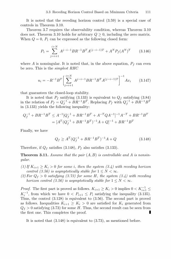
3.3 Receding Horizon Control Based on Minimum Criteria 111

It is noted that the receding horizon control (3.59) is a special case ofcontrols in Theorem 3.10.

Theorem 3.7 requires the observability condition, whereas Theorem 3.10does not. Theorem 3.10 holds for arbitrary Q ≥ 0, including the zero matrix.When Q = 0, P1 can be expressed as the following closed form:

P1 =i+N∑

j=i+1

Aj−i−1BR−1BT A(j−i−1)T + ANPf (AN )T (3.146)

where A is nonsingular. It is noted that, in the above equation, Pf can evenbe zero. This is the simplest RHC

ui = −R−1BT

[ i+N∑j=i+1

Aj−i−1BR−1BT A(j−i−1)T

]−1

Axi (3.147)

that guarantees the closed-loop stability.It is noted that Pf satifying (3.133) is equivalent to Qf satisfying (3.84)

in the relation of Pf = Q−1f + BR−1BT . Replacing Pf with Q−1

f + BR−1BT

in (3.133) yields the following inequality:

Q−1f + BR−1BT ≤ A−1[Q−1

f + BR−1BT + A−T QA−1]−1A−T + BR−1BT

= [AT (Q−1f + BR−1BT )−1A + Q]−1 + BR−1BT

Finally, we have

Qf ≥ AT (Q−1f + BR−1BT )−1A + Q (3.148)

Therefore, if Qf satisfies (3.148), Pf also satisfies (3.133).

Theorem 3.11. Assume that the pair (A,B) is controllable and A is nonsin-gular.

(1) If Ki+1 ≥ Ki > 0 for some i, then the system (3.4) with receding horizoncontrol (3.56) is asymptotically stable for 1 ≤ N < ∞.

(2) For Qf > 0 satisfying (3.73) for some H, the system (3.4) with recedinghorizon control (3.56) is asymptotically stable for 1 ≤ N < ∞.

Proof. The first part is proved as follows. Ki+1 ≥ Ki > 0 implies 0 < K−1i+1 ≤

K−1i , from which we have 0 < Pi+1 ≤ Pi satisfying the inequality (3.135).

Thus, the control (3.128) is equivalent to (3.56). The second part is provedas follows. Inequalities Ki+1 ≥ Ki > 0 are satisfied for Ki generated fromQf > 0 satisfying (3.73) for some H. Thus, the second result can be seen fromthe first one. This completes the proof.

It is noted that (3.148) is equivalent to (3.73), as mentioned before.

112 3 State Feedback Receding Horizon Controls

So far, the cost monotonicity condition has been introduced for stability.Without this cost monotonicity condition, there still exists a finite horizonsuch that the resulting receding horizon control stabilizes the closed-loop sys-tems.

Before proceeding to the main theorem, we introduce a matrix norm‖A‖ρ,ε, which satisfies the properties of the norm and ρ(A) ≤ ‖A‖ρ,ε ≤ρ(A) + ε. Here, ε is a design parameter and ρ(A) is the spectral radius ofA, i.e. ρ(A) = max1≤i≤n |λi|.

Theorem 3.12. Suppose that Q ≥ 0 and R > 0. If the pairs (A,B) and(A,Q

12 ) are controllable and observable respectively, then the receding horizon

control (3.56) for the free terminal cost stabilizes the systems for the followinghorizon:

N > 1 +1

ln ‖ATc ‖ρ,ε + ln ‖Ac‖ρ,ε

ln[

1β‖BR−1BT ‖ρ,ε

1

‖Ac‖ρ,ε− 1 − ε

](3.149)

where β = ‖Qf −K∞‖ρ,ε, Ac = A−BR−1BT [I +K∞BR−1BT ]−1K∞A, andK∞ is the solution to the steady-state Riccati equation.

Proof. Denote Ki,N by Ki,N − K∞, where Ki,N is the solution at timei to the Riccati equation starting from time N , and K∞ is the steady-statesolution to the Riccati equation which is given by (2.108). In order to enhancethe clarification, Ki,N is used instead of Ki. KN,N = Qf and K1,N of i = 1are involved with the control gain of the RHC with a horizon size N . Fromproperties of the Riccati equation, we have the following inequality:

Ki,N ≤ ATc Ki+1,NAc (3.150)

Taking the norm ‖ · ‖ρ,ε on both sides of (3.150), we obtain

‖Ki,N‖ρ,ε ≤ ‖ATc ‖ρ,ε‖Ki+1,N‖ρ,ε‖Ac‖ρ,ε (3.151)

where a norm ‖ · ‖ρ,ε is defined just before this theorem. From (3.151), it canbe easily seen that ‖K1,N‖ρ,ε is bounded below as follows:

‖K1,N‖ρ,ε ≤ ‖ATc ‖N−1

ρ,ε ‖KN,N‖ρ,ε‖Ac‖N−1ρ,ε = ‖AT

c ‖N−1ρ,ε β‖Ac‖N−1

ρ,ε (3.152)

The closed-loop system matrix Ac,N from the control gain K1,N is givenby

Ac,N = A − BR−1BT [I + K1,NBR−1BT ]−1K1,NA (3.153)

It is known that the steady-state closed-loop system matrices Ac and Ac,N in(3.153) are related to each other as follows:

Ac,N =[I + BR−1

o,NBTK1,N

]Ac (3.154)

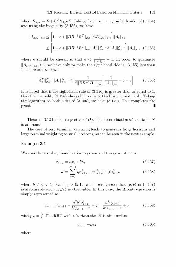
3.3 Receding Horizon Control Based on Minimum Criteria 113

where Ro,N = R+BT K1,NB. Taking the norm ‖·‖ρ,ε on both sides of (3.154)and using the inequality (3.152), we have

‖Ac,N‖ρ,ε ≤[1 + ε + ‖BR−1BT ‖ρ,ε‖K1,N‖ρ,ε

]‖Ac‖ρ,ε

≤[1 + ε + ‖BR−1BT ‖ρ,ε‖AT

c ‖N−1ρ,ε β‖Ac‖N−1

ρ,ε

]‖Ac‖ρ,ε (3.155)

where ε should be chosen so that ε < 1‖Ac‖ρ,ε

− 1. In order to guarantee‖Ac,N‖ρ,ε < 1, we have only to make the right-hand side in (3.155) less than1. Therefore, we have

‖ATc ‖N−1

ρ,ε ‖Ac‖N−1ρ,ε ≤ 1

β‖BR−1BT ‖ρ,ε

[1

‖Ac‖ρ,ε− 1 − ε

](3.156)

It is noted that if the right-hand side of (3.156) is greater than or equal to 1,then the inequality (3.156) always holds due to the Hurwitz matrix Ac. Takingthe logarithm on both sides of (3.156), we have (3.149). This completes theproof.

Theorem 3.12 holds irrespective of Qf . The determination of a suitable Nis an issue.

The case of zero terminal weighting leads to generally large horizons andlarge terminal weighting to small horizons, as can be seen in the next example.

Example 3.1

We consider a scalar, time-invariant system and the quadratic cost

xi+1 = axi + bui (3.157)

J =N−1∑j=0

[qx2k+j + ru2

k+j ] + fx2k+N (3.158)

where b = 0, r > 0 and q > 0. It can be easily seen that (a, b) in (3.157)is stabilizable and (a,

√q) is observable. In this case, the Riccati equation is

simply represented as

pk = a2pk+1 −a2b2p2

k+1

b2pk+1 + r+ q =

a2rpk+1

b2pk+1 + r+ q (3.159)

with pN = f . The RHC with a horizon size N is obtained as

uk = −Lxk (3.160)

where

114 3 State Feedback Receding Horizon Controls

L =abp1

b2p1 + r(3.161)

Now, we investigate the horizon of the RHC for stabilizing the closed-loopsystem. The steady-state solution to the ARE and the system matrix of theclosed-loop system can be written as

p∞ =q

2Π

[±√

(1 − Π)2 +4Π

1 − a2− (1 − Π)

](3.162)

acl = a − bL =a

1 + b2

r p∞(3.163)

where

Π =b2q

(1 − a2)r(3.164)

We will consider two cases. One is for a stable system and the other for anunstable system.

(1) Stable system ( |a| < 1 )Since |a| < 1, 1 − a2 > 0 and Π > 0. In this case, we have the positivesolution as

p∞ =q

2Π

[√(1 − Π)2 +

4Π1 − a2

− (1 − Π)]

(3.165)

From (3.163), we have |acl| < |a| < 1. So, the asymptotical stability isguaranteed for the closed-loop system.

(2) Unstable system ( |a| > 1 )Since |a| > 1, 1 − a2 < 0 and Π < 0. In this case, we have the positivesolution given by

p∞ = − q

2Π

[√(1 − Π)2 +

4Π1 − a2

+ (1 − Π)]

(3.166)

The system matrix acl of the closed-loop system can be represented as

acl =a

1 − 1−a2

2

[√(1 − Π)2 + 4Π

1−a2 + 1 − Π] (3.167)

We have |acl| < 1 from the following relation:

|2 +√

((a2 − 1)(1 − Π) + 2)2 − 4a2 + (a2 − 1)(1 − Π)|> |2 +

√(a2 + 1)2 − 4a2 + (a2 − 1)|

= |2a2| > 2|a|.

3.3 Receding Horizon Control Based on Minimum Criteria 115

From acl, the lower bound of the horizon size guaranteeing the stability isobtained as

N > 1 +1

2 ln |acl| ln[

r

b2|f − p∞|

1

|acl| − 1]

(3.168)

where ε = 0 and absolute values of scalar values are used for ‖ · ‖ρ,ε norm.

As can be seen in this example, the gain and phase margins of the RHCare greater than those of the conventional steady-state LQ control. For thegeneral result on multi-input–multi-output systems, this is left as an exercise.

3.3.5 Additional Properties of Receding Horizon Linear QuadraticControl

A Prescribed Degree of Stability

We introduce another performance criterion to make closed-loop eigenvaluessmaller than a specific value. Of course, as closed-loop eigenvalues get smaller,the closed-loop system becomes more stable, probably with an excessive con-trol energy cost.

Consider the following performance criterion:

J =N−1∑j=0

α2j(uTk+jRuk+j + xT

k+jQxk+j) + α2NxTk+NQfxk+N (3.169)

where α > 1 and the pair (A,B) is stabilizable.The first thing we have to do for dealing with (3.169) is to make transfor-

mations that convert the given problem to a standard LQ problem. Therefore,we introduce new variables such as

xk+j= αjxk+j (3.170)

uk+j= αjuk+j (3.171)

Observing that

xk+j+1 = αj+1xk+j+1 = ααj [Axk+j + Buk+j ] = αAxk+j + αBuk+j (3.172)

we may associate the system (3.172) with the following performance criterion:

J =N−1∑j=0

(uTk+jRuk+j + xT

k+jQxk+j) + xTk+NQf xk+N (3.173)

The receding horizon control for (3.172) and (3.173) can be written as

uk = −R−1αBT [I + K1αBR−1αBT ]−1K1αAxk (3.174)

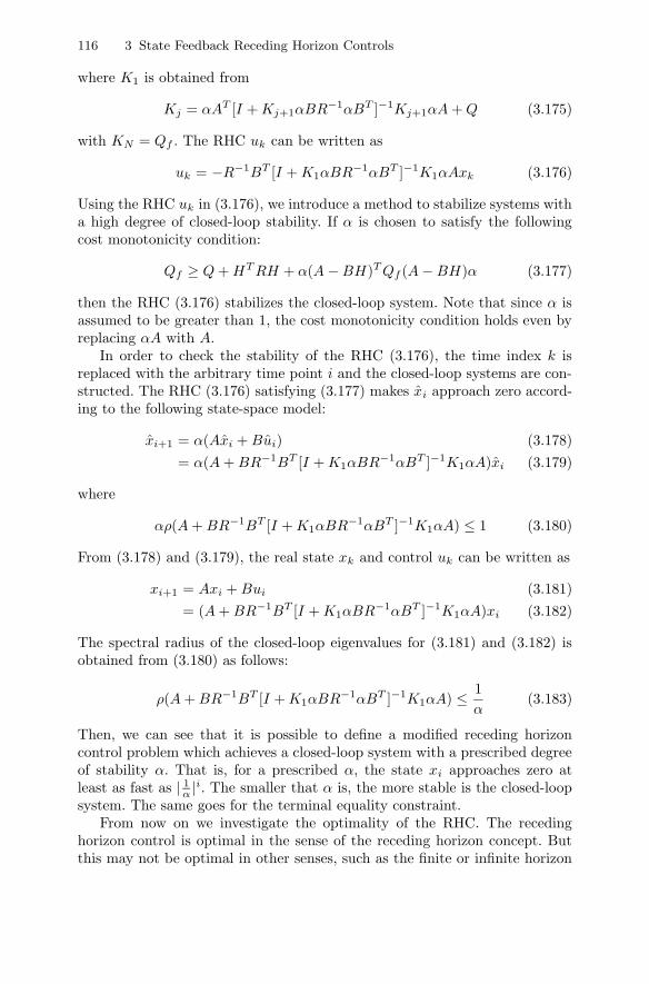
116 3 State Feedback Receding Horizon Controls

where K1 is obtained from

Kj = αAT [I + Kj+1αBR−1αBT ]−1Kj+1αA + Q (3.175)

with KN = Qf . The RHC uk can be written as

uk = −R−1BT [I + K1αBR−1αBT ]−1K1αAxk (3.176)

Using the RHC uk in (3.176), we introduce a method to stabilize systems witha high degree of closed-loop stability. If α is chosen to satisfy the followingcost monotonicity condition:

Qf ≥ Q + HT RH + α(A − BH)T Qf (A − BH)α (3.177)

then the RHC (3.176) stabilizes the closed-loop system. Note that since α isassumed to be greater than 1, the cost monotonicity condition holds even byreplacing αA with A.

In order to check the stability of the RHC (3.176), the time index k isreplaced with the arbitrary time point i and the closed-loop systems are con-structed. The RHC (3.176) satisfying (3.177) makes xi approach zero accord-ing to the following state-space model:

xi+1 = α(Axi + Bui) (3.178)= α(A + BR−1BT [I + K1αBR−1αBT ]−1K1αA)xi (3.179)

where

αρ(A + BR−1BT [I + K1αBR−1αBT ]−1K1αA) ≤ 1 (3.180)

From (3.178) and (3.179), the real state xk and control uk can be written as

xi+1 = Axi + Bui (3.181)= (A + BR−1BT [I + K1αBR−1αBT ]−1K1αA)xi (3.182)

The spectral radius of the closed-loop eigenvalues for (3.181) and (3.182) isobtained from (3.180) as follows:

ρ(A + BR−1BT [I + K1αBR−1αBT ]−1K1αA) ≤ 1α

(3.183)

Then, we can see that it is possible to define a modified receding horizoncontrol problem which achieves a closed-loop system with a prescribed degreeof stability α. That is, for a prescribed α, the state xi approaches zero atleast as fast as | 1

α |i. The smaller that α is, the more stable is the closed-loopsystem. The same goes for the terminal equality constraint.

From now on we investigate the optimality of the RHC. The recedinghorizon control is optimal in the sense of the receding horizon concept. Butthis may not be optimal in other senses, such as the finite or infinite horizon

3.3 Receding Horizon Control Based on Minimum Criteria 117

Fig. 3.8. Effect of parameter α

optimal control concept. Likewise, standard finite or infinite optimal controlmay not be optimal in the sense of the receding horizon control, whereas itis optimal in the sense of the standard optimal control. Therefore, it will beinteresting to compare between them.

For simplicity we assume that there is no reference signal to track.

Theorem 3.13. The standard quadratic performance criterion for the sys-tems with the receding horizon control (3.59) under a terminal equality con-straint has the following performance bounds:

xi0Ki0,ifxi0 ≤

if−1∑i=i0

[xTi Qxi + uT

i Rui] ≤ xTi0P

−10 xi0 (3.184)

Proof. We have the following inequality:

xTi P−1

0 xi − xTi+1P

−10 xi+1 = xT

i P−1−1 xi − xT

i+1P−10 xi+1 + xT

i [P−10 − P−1

−1 ]xi

≥ xTi P−1

−1 xi − xTi+1P

−10 xi+1 (3.185)

which follows from the fact that P−10 ≥ P−1

−1 . By using the optimality, we have

xTi P−1

−1 xi − xTi+1P

−10 xi+1 = J∗(xi, i, i + N + 1) − J∗(xi+1, i + 1, i + N + 1)

≥ J∗(xi, i, i + N + 1) − J(xi+1, i + 1, i + N + 1)≥ xT

i Qxi + uiRui (3.186)

where J(xi+1, i + 1, i + N + 1) is a cost function generated from the statedriven by the optimal control that is based on the interval [i, i+N +1]. From(3.186) we have

118 3 State Feedback Receding Horizon Controls

if−1∑i=i0

[xTi Qxi + uT

i Rui] ≤ xTi0P

−10 xi0 − xT

ifP−1

0 xif≤ xT

i0P−10 xi0 (3.187)

The lower bound is obvious. This completes the proof.

The next theorem introduced is for the case of the free terminal cost.

Theorem 3.14. The standard quadratic performance criterion for the sys-tems with the receding horizon control (3.56) under a cost monotonicity con-dition (3.73) has the following performance bounds:

xi0Ki0,ifxi0 ≤

if−1∑i=i0

[xTi Qxi + uT

i Rui] + xTif

Qfxif

≤ xTi0 [K0 + Θ(if−i0)T QfΘif−i0 ]xi0

where

Θ= A − BR−1BT K1[I + BR−1BT K1]−1A

K0 is obtained from (3.47) starting from KN = Qf , and Ki0,ifis obtained by

starting from Kif ,if= Qf .

Proof. The lower bound is obvious, since Ki0,ifis the cost incurred by the

standard optimal control law. The gain of the receding horizon control is givenby

L= R−1BT K1[I + BR−1BT K1]−1A

= [R + BT K1B]−1BT K1A.

As is well known, the quadratic cost for the feedback control ui = −Lxi isgiven by

if−1∑i=i0

[xTi Qxi + uT

i Rui] + xTif

Qfxif= xT

i0Ni0xi0

where Ni is the solution of the following difference equation:

Ni = [A − BL]T Ni+1[A − BL] + LT RL + Q

Nif= Qf

From (3.47) and (3.48) we have

Ki = AT Ki+1A − AT Ki+1B[R + BT Ki+1B]−1BT Ki+1A + Q

where KN = Qf . If we note that, for i = 0 in (3.188),

3.3 Receding Horizon Control Based on Minimum Criteria 119

AT K1B[R + BT K1B]−1BT K1A = AT K1BL = LT BT K1A

= LT [R + BT K1B]L

we can easily have

K0 = [A − BL]T K1[A − BL] + LT RL + Q

Let

Ti= Ni − K0

then Ti satisfies

Ti = [A − BL]T [Ti+1 − Ti][A − BL] ≤ [A − BL]T Ti+1[A − BL]

with the boundary condition Tif= Qif

−K0, where Ti = K1 −K0 ≥ 0 undera cost monotonicity condition. We can obtain Ti0 by evaluating recursively,and finally we have

Ti0 ≤ Θ(if−i0)T TifΘif−i0

where Θ = A − BL. Thus, we have

Ni0 ≤ K0 + Θ(if−i0)T [Qif− K0]Θif−i0

from which follows the result. This completes the proof.

Since Θ(if−i0)T → 0, the infinite time cost has the following bounds:

xTi0Ki0,∞xi0 ≤

∞∑i=0

xTi Qxi + uT

i Rui (3.188)

≤ xTi0K0xi0 (3.189)

The receding horizon control is optimal in its own right. However, the recedinghorizon control can be used for a suboptimal control for the standard regula-tion problem. In this case, Theorem 3.14 provides a degree of suboptimality.

Example 3.2

In this example, it is shown via simulation that the RHC has good track-ing ability for the nonzero reference signal. For simulation, we consider atwo-dimensional free body system. This free body is moved by two kinds offorces, i.e. a horizontal force and a vertical force. According to Newton’s laws,the following dynamics are obtained:

Mx + Bx = ux

Mx + By = uy

120 3 State Feedback Receding Horizon Controls

where M , B, x, y, ux, and uy are the mass of the free body, the frictioncoefficient, the horizontal position, the vertical position, the horizontal force,and the vertical force respectively. Through plugging the real values into theparameters and taking the discretization procedure, we have

xk+1 =

⎡⎢⎢⎣1 0.0550 0 00 0.9950 0 00 0 1 0.05500 0 0 0.9995

⎤⎥⎥⎦xk +

⎡⎢⎢⎣0.0015 00.0550 0

0 0.00150 0.0550

⎤⎥⎥⎦uk

yk =[

1 0 0 00 0 1 0

]xk

where the first and second components of xi denote the positions of x and yrespectively, and the two components of ui are for the horizontal and verticalforces.

The sampling time and the horizon size are taken as 0.055 and 3. Thereference signal is given by

xri =

⎧⎪⎪⎪⎪⎨⎪⎪⎪⎪⎩1 − i

100 0 ≤ i < 1000 100 ≤ i < 200

i100 − 2 200 ≤ i < 3001 300 ≤ i < 4001 i ≥ 400

yri =

⎧⎪⎪⎪⎪⎨⎪⎪⎪⎪⎩1 0 ≤ i < 1002 − i

100 100 ≤ i < 2000 200 ≤ i < 300

i100 − 3 300 ≤ i < 4001 i ≥ 400

Q and R for the LQ and receding horizon controls are chosen to be unit ma-trices. The final weighting matrix for the RHC is set to 105I. In Figure 3.9,we can see that the RHC has the better performance for the given referencetrajectory. Actually, the trajectory for the LQTC is way off the reference sig-nal. However, one for the RHC keeps up with the reference well.

Prediction Horizon

In general, the horizon N in the performance criterion (3.22) is divided intotwo parts, [k, k+Nc−1] and [k+Nc, k+N ]. The control on [k, k+Nc−1] isobtained optimally to minimize the performance criterion on [k, k + Nc − 1],while the control on [k + Nc, k + N ] is usually a given control, say a linearcontrol ui = Hxi on this horizon. In this case, the horizon or horizon sizeNc is called the control horizon and N is called the prediction horizon, theperformance horizon, or the cost horizon. Here, N can be denoted as Np toindicate the prediction horizon. In the previous problem we discussed so far,the control horizon Nc was the same as the prediction horizon Np. In thiscase, we will use the term control horizon instead of prediction horizon. Weconsider the following performance criterion:

3.3 Receding Horizon Control Based on Minimum Criteria 121

−0.2 0 0.2 0.4 0.6 0.8 1 1.2−0.2

0

0.2

0.4

0.6

0.8

1

1.2

RHC

LQTC

(a) Phase plot

0 50 100 150 200 250 300 350 400 450−0.2

0

0.2

0.4

0.6

0.8

1

1.2

RHC

LQTC

(b) State trajectory

Fig. 3.9. Comparison RHC and LQTC

J =Nc−1∑j=0

(uTk+jRuk+j + xT

k+jQxk+j) +Np∑

j=Nc

(uTk+jRuk+j

+ xTk+jQxk+j) (3.190)

where the control horizon and the prediction horizon are [k, k + Nc − 1] and[k, k +Np] respectively. If we apply a linear control ui = Hxi on [k +Nc, k +Np], we have

122 3 State Feedback Receding Horizon Controls

J =Nc−1∑j=0

[xTk+jQxk+j + uT

k+jRuk+j ]

+ xTk+Nc

⎧⎨⎩Np∑

j=Nc

((A − HB)T )j−Nc [Q + HT RH](A − BH)j−Nc

⎫⎬⎭xk+Nc

=Nc−1∑j=0

[xTk+jQxk+j + uT

k+jRuk+j ] + xTk+Nc

Qfxk+Nc(3.191)

where

Qf =Np∑

j=Nc

((A − HB)T )j−Nc [Q + HT RH](A − BH)j−Nc (3.192)

This is particularly important when Np = ∞ with linear stable control, sincethis approach is sometimes good for constrained and nonlinear systems. Butwe may lose good properties inherited from a finite horizon. For linear systems,the infinite prediction horizon can be reduced to the finite one, which is thesame as the control horizon. The infinite prediction horizon can be changedas

J =∞∑

j=0

[xTk+jQxk+j + uT

k+jRuk+j ]

=Nc−1∑j=0

[xTk+jQxk+j + uT

k+jRuk+j ] + xTk+Nc

Qfxk+Nc(3.193)

where Qf satisfies Qf = Q + HT RH + (A − BH)T Qf (A − BH). Therefore,Qf is related to the terminal weighting matrix.

3.3.6 A Special Case of Input–Output Systems

In addition to the state-space model (3.1) and (3.2), GPC has used the fol-lowing CARIMA model:

A(q−1)yi = B(q−1)ui−1 (3.194)

where

A(q−1) = 1 + a1q−1 + · · · + anq−n, an = 0 (3.195)

B(q−1) = b1 + b2q−1 + · · · + bmq−m+1 (3.196)

where q−1 is the unit delay operator, such as q−1yi = yi−1, and ui =(1 − q−1)ui = ui − ui−1. It is noted that B(q−1) can be

3.3 Receding Horizon Control Based on Minimum Criteria 123

b1 + b2q−1 + · · · + bnq−n+1, m ≤ n (3.197)

where bi = 0 for i > m. It is noted that (3.194) can be represented as

A(q−1)yi = B(q−1)ui (3.198)

where

B(q−1) = b1q−1 + b2q

−2 · · · + bnq−n (3.199)

The above model (3.198) in an input–output form can be transformed to thestate-space model

xi+1 = Axi + Bui

yi = Cxi (3.200)

where xi ∈ Rn and

A =

⎡⎢⎢⎢⎢⎢⎣−a1 1 0 · · · 0−a2 0 1 · · · 0

......

.... . .

...−an−1 0 0 · · · 1−an 0 0 · · · 0

⎤⎥⎥⎥⎥⎥⎦ B =

⎡⎢⎢⎢⎢⎢⎣b1

b2

...bn−1

bn

⎤⎥⎥⎥⎥⎥⎦ (3.201)

C =[1 0 0 · · · 0

]It is clear that yi = xi

(1), where xi(1) indicates the first element of xi.

The common performance criterion for the CARIMA model (3.194) isgiven as

Nc∑j=1

[q(yk+j − yr

k+j)2 + r(uk+j−1)2

](3.202)

Here, Nc is the control horizon.Since yk is given, the optimal control for (3.202) is also optimal for the

following performance index:

Nc−1∑j=0

[q(yk+j − yr

k+j)2 + r(uk+j)2

]+ q(yk+Nc

− yrk+Nc

)2 (3.203)

The performance index (3.202) can be extended to include a free terminalcost such as

Nc∑j=1

[q(yk+j − yr

k+j)2 + r(uk+j−1)2

]+

Np∑j=Nc+1

qf (yk+j − yrk+j)

2 (3.204)

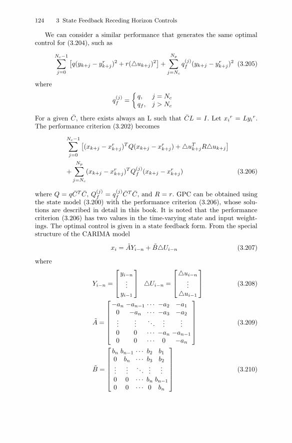
124 3 State Feedback Receding Horizon Controls

We can consider a similar performance that generates the same optimalcontrol for (3.204), such as

Nc−1∑j=0

[q(yk+j − yr

k+j)2 + r(uk+j)2

]+

Np∑j=Nc

q(j)f (yk+j − yr

k+j)2 (3.205)

where

q(j)f =

q, j = Nc

qf , j > Nc

For a given C, there exists always an L such that CL = I. Let xir = Lyi

r.The performance criterion (3.202) becomes

Nc−1∑j=0

[(xk+j − xr

k+j)T Q(xk+j − xr

k+j) + uTk+jRuk+j

]+

Np∑j=Nc

(xk+j − xrk+j)

T Q(j)f (xk+j − xr

k+j) (3.206)

where Q = qCT C, Q(j)f = q

(j)f CT C, and R = r. GPC can be obtained using

the state model (3.200) with the performance criterion (3.206), whose solu-tions are described in detail in this book. It is noted that the performancecriterion (3.206) has two values in the time-varying state and input weight-ings. The optimal control is given in a state feedback form. From the specialstructure of the CARIMA model

xi = AYi−n + BUi−n (3.207)

where

Yi−n =

⎡⎢⎣ yi−n

...yi−1

⎤⎥⎦ Ui−n =

⎡⎢⎣ui−n

...ui−1

⎤⎥⎦ (3.208)

A =

⎡⎢⎢⎢⎢⎢⎣−an −an−1 · · · −a2 −a1

0 −an · · · −a3 −a2

......

. . ....

...0 0 · · · −an −an−1

0 0 · · · 0 −an

⎤⎥⎥⎥⎥⎥⎦ (3.209)

B =

⎡⎢⎢⎢⎢⎢⎣bn bn−1 · · · b2 b1

0 bn · · · b3 b2

......

. . ....

...0 0 · · · bn bn−1

0 0 · · · 0 bn

⎤⎥⎥⎥⎥⎥⎦ (3.210)

3.4 Receding Horizon Control Based on Minimax Criteria 125

the state can be computed with input control and measured output. Theoptimal control can be given as an output feedback control.

If uk+Nc= ... = uk+Np−1 = 0 is assumed, for Np = Nc + n − 1, then

the terminal cost can be represented as

Np∑j=Nc

q(j)f (yk+j − yr

k+j)2

= (Yk+Nc− Y r

k+Nc)T Qf (Yk+Nc

− Y rk+Nc

) (3.211)

where

Qf =[diag(

Np−Nc+1︷ ︸︸ ︷q qf · · · qf )

], Y r

k+Nc=

⎡⎢⎣ yrk+Nc

...yr

k+Nc+n−1

⎤⎥⎦ (3.212)

In this case the terminal cost becomes

(xk+Nc+n − AY rk+Nc

)T (AT )−1Qf˜A−1(xk+Nc+n − AY r

k+Nc)

= (xk+Nc− xr

k+Nc)T Qf (xk+Nc

− xrk+Nc

)

where

Qf = qf (AT )n(AT )−1Qf A−1An (3.213)

xrk+Nc

= (An)−1AY rk+Nc

(3.214)

It is noted that A and A are all nonsingular.The performance criterion (3.204) is for the free terminal cost. We can

now introduce a terminal equality constraint, such as

yk+j = yrk+j , j = Nc, · · · , Np (3.215)

which is equivalent to xk+Nc= xr

k+Nc. GPC can be obtained from the results

in state-space forms that have already been discussed.

3.4 Receding Horizon Control Based on MinimaxCriteria

3.4.1 Receding Horizon H∞ Control

In this section, a receding horizon H∞ control in a tracking form for discretetime-invariant systems is obtained.

Based on the following system in a predictive form:

xk+j+1 = Axk+j + Bwwk+j + Buk+j (3.216)zk+j = Czxk+j (3.217)

126 3 State Feedback Receding Horizon Controls

with the initial state xk, the optimal control and the worst-case disturbancecan be written in a predictive form as

u∗k+j = −R−1BT Λ−1

k+j+1,if[Mk+j+1,if

Axk+j + gk+j+1,if]

w∗k+j = γ−2R−1

w BTwΛ−1

k+j+1,if[Mk+j+1,if

Axk+j + gk+j+1,if]

Mk+j,ifand gk+j,if

can be obtained from

Mk+j,if= AT Λ−1

k+j+1,ifMk+j+1,if

A + Q, i = i0, · · · , if − 1 (3.218)

Mif ,if= Qf (3.219)

and

gk+j,if= −AT Λ−1

k+j+1,ifgk+j+1,if

− Qxrk+j (3.220)

g if ,if= −Qfxr

if(3.221)

whereΛk+j+1,if

= I + Mk+j+1,if(BR−1BT − γ−2BwR−1

w BTw)

If we replace if with k +N , the optimal control on the interval [k, k +N ]is given by

u∗k+j = −R−1BT Λ−1

k+j+1,k+N [Mk+j+1,k+NAxk+j + gk+j+1,k+N ]

w∗k+j = γ−2R−1

w BTwΛ−1

k+j+1,k+N [Mk+j+1,k+NAxk+j + gk+j+1,k+N ]

The receding horizon control is given by the first control, j = 0, at eachinterval as

u∗k = −R−1BT Λ−1

k+1,t+N [Mk+1,k+NAxk + gk+1,k+N ]

w∗k = γ−2R−1

w BTwΛ−1

k+1,k+N [Mk+1,k+NAxk + gk+1,k+N ]

Replace k with i as an arbitrary time point for discrete-time systems to obtain

u∗i = −R−1BT Λ−1

i+1,i+N [Mi+1,i+NAxi + gi+1,i+N ]

w∗i = γ−2R−1

w BTwΛ−1

i+1,i+N [Mi+1,i+NAxi + gi+1,i+N ].

In case of time-invariant systems, the simplified forms are obtained as

u∗i = −R−1BT Λ−1

1 [M1Axi + gi+1,i+N ] (3.222)w∗

i = γ−2R−1w BT

wΛ−11 [M1Axi + gi+1,i+N ] (3.223)

M1 and gi,i+N can be obtained from

Mj = AT Λ−1j+1Mj+1A + Q, j = 1, · · · , N − 1 (3.224)

MN = Qf (3.225)

3.4 Receding Horizon Control Based on Minimax Criteria 127

and

gj,i+N = −AT Λ−1j+1gj+1,i+N − Qxr

j (3.226)gi+N,i+N = −Qfxr

i+N (3.227)

whereΛj+1 = I + Mj+1(BR−1BT − γ−2BwR−1

w BTw)

Recall through this chapter that the following condition is assumed to besatisfied:

Rw − γ−2BTwMiBw > 0 , i = 1, · · · , N (3.228)

in order to guarantee the existence of the saddle point. Note that from (3.228),we have M−1

i > γ−2BwR−1w BT

w , from which the positive definiteness of Λ−1i Mi

is guaranteed. The positive definiteness of Mi is also guaranteed with theobservability of (A,Q

12 ).

From (2.152) and (2.153) we have another form of the receding horizonH∞ control:

u∗i = −R−1BT P−1

1 Axi (3.229)w∗

i = γ−2R−1w BT

wP−11 Axi (3.230)

where Π = BR−1B − γ−2BwR−1w BT

w ,

Pi = A−1Pi+1[I + A−1QA−1Pi+1]−1A−1 + Π (3.231)

and the boundary condition PN = M−1N + Π = Q−1

f + Π.

We can use the following forward computation: by using the new variables−→M j and

−→Λ j such that

−→M j = MN−j and

−→Λ j = ΛN−j , (3.222) and (3.223) can

be written as

u∗i = −R−1BT−→Λ−1

N−1[−→MN−1Axi + gi+1,i+N ] (3.232)

w∗i = γ−2R−1

w BTw

−→Λ−1

N−1[−→MN−1Axi + gi+1,i+N ] (3.233)

where−→M j = AT−→Λ−1

j

−→M j−1A + Q, j = 1, · · · , N − 1

−→M0 = Qf

−→Λ j = I +

−→M j(BR−1BT − γ−2BwR−1

w BTw)

128 3 State Feedback Receding Horizon Controls

3.4.2 Monotonicity of the Saddle-point Optimal Cost

In this section, terminal inequality conditions are proposed for linear discretetime-invariant systems which guarantee the monotonicity of the saddle-pointvalue. In the next section, under the proposed terminal inequality conditions,the closed-loop stability of RHC is shown for linear discrete time-invariantsystems.

Theorem 3.15. Assume that Qf in (3.219) satisfies the following inequality:

Qf ≥ Q + HT RH − ΓT RwΓ + ATclQfAcl for some H ∈ m×n (3.234)

where

Acl = A − BH + BwΓ

Γ = γ−2R−1w BT

wΛ−1QfA (3.235)Λ = I + Qf (BR−1BT − γ−2BwR−1

w BTw) (3.236)

The saddle-point optimal cost J∗(xi, i, if ) in (3.16) then satisfies the followingrelation:

J∗(xτ , τ, σ + 1) ≤ J∗(xτ , τ, σ), τ ≤ σ (3.237)

and thus Mτ,σ+1 ≤ Mτ,σ.

Proof. Subtracting J∗(xτ , τ, σ) from J∗(xτ , τ, σ + 1), we can write

δJ∗(xτ , σ) =σ∑

i=τ

[x1Ti Qx1

i + u1Ti Ru1

i − γ2w1Ti Rww1

i ] + x1Tσ+1Qfx1

σ+1 (3.238)

−σ−1∑i=τ

[x2Ti Qx2

i + u2Ti Ru2

i − γ2w2Ti Rww2

i ] − x2Tσ Qfx2

σ (3.239)

where the pair u1i and w1

i is a saddle-point solution for J(xτ , τ, σ +1) and thepair u2

i and w2i is one for J(xτ , τ, σ). If we replace u1

i by u2i and w2

i by w1i up

to σ − 1, the following inequalities are obtained by J(u∗, w∗) ≤ J(u,w∗):

σ∑i=τ

[x1Ti Qx1

i + u1Ti Ru1

i − γ2w1Ti Rww1

i ] + x1Tσ+1Qfx1

σ+1

≤σ−1∑i=τ

[xTi Qxi + u2T

i Ru2i − γ2w1T

i Rww1i ] + xT

σ Qxσ + u1Tσ Ru1

σ − γ2w1Tσ Rww1

σ

+ x1Tσ+1Qfx1

σ+1

where u1σ = Hxσ, and w1

σ = Γ xσ. By J(u∗, w∗) ≥ J(u∗, w), we have

3.4 Receding Horizon Control Based on Minimax Criteria 129

σ−1∑i=τ

[x2Ti Qx2

i + u2Ti Ru2

i − γ2w2Ti Rww2

i ] + xTσ Qfxσ

≥σ−1∑i=τ

[xTi Qxi + u2T

i Ru2i − γ2w1T

i Rww1i ] + xT

σ Qf xσ

Note that xi is a trajectory associated with u2i and w1

i . We have the followinginequality:

δJ∗(xτ , σ) ≤ xTσ Q + HT RH − ΓT RwΓ + AT

clQfAcl − Qfxσ ≤ 0 (3.240)

where the last inequality comes from (3.234).Since δJ∗(xτ , σ) = xT

τ [Mτ,σ+1 − Mτ,σ]xτ ≤ 0 for all xτ , we have thatMτ,σ+1 − Mτ,σ ≤ 0. For time-invariant systems we have

Mτ+1 ≤ Mτ (3.241)

This completes the proof.

Note that Qf satisfying the inequality (3.234) in (3.15) should be checkedfor whether Mi,if

generated from the boundary value Qf satisfies Rw −γ−2BT

wMi,ifBw. In order to obtain a feasible solution Qf , Rw and γ can

be adjusted.

Case 1: Γ in the inequality (3.234) includes Qf , which makes it difficultto handle the inequality. We introduce the inequality without the variable Γas follows:

Q + HT RH − ΓT RwΓ + ATclQfAcl

= Q + HT RH + ΣT (BTwQfBw − Rw)Σ

− (A − BH)T QfBw(BTwQfBw − Rw)−1BwQf (A − BH),

≤ Q + HT RH − (A − BH)T (BTwQfBw − Rw)−1(A − BH) ≤ Qf (3.242)

where Σ = Γ + (BTwQfBw − R)−1BT

wQf (A − BH).

Case 2:

Qf ≥ AT Qf [I + ΠQf ]−1A + Q (3.243)

where Π = BR−1B − γ−2BwR−1w Bw.

If H is replaced by an optimal gain H = −R−1BT [I +QfΠ]−1 Qf A, thenby using the matrix inversion lemma in Appendix A, we can have (3.243). Itis left as an exercise at the end of this chapter.

130 3 State Feedback Receding Horizon Controls

Case 3:

Qf = Q + HT RH − ΓT RwΓ + ATclQfAcl (3.244)

which is a special case of (3.234). Qf has the following meaning. If the pair(A,B) is stabilizable and the system is asymptotically stable with ui = −Hxi

and wi = γ−1BTγ [I + Mi+1,∞Q]−1Mi+1,∞Axi for σ ≥ i ≥ τ , then

minui,i∈[τ,σ−1]

∞∑i=τ

[xTi Qxi + uT

i Rui − γ2wTi Rwwi]

= minui,i∈[τ,σ−1]

σ−1∑i=τ

[xTi Qxi + uT

i Rui − γ2wTi Rwwi] + xT

σ Qfxσ (3.245)

where Qf can be shown to satisfy (3.244).

Case 4:

Qf = Q − Γ T RwΓ + [A + BwΓ ]T Qf [A + BwΓ ] (3.246)

which is also a special case of (3.234). If the system matrix A is stable withui = 0 and wi = γ−1R−1

w BTw [I + Mi+1,∞Q]−1Mi+1,∞Axi for σ ≥ i ≥ τ then,

Qf satisfies (3.246).In the following, the nondecreasing monotonicity of the saddle-point opti-

mal cost is studied.

Theorem 3.16. Assume that Qf in (3.16) satisfies the following inequality:

Qf ≤ AT Qf [I + ΠQf ]−1A + Q (3.247)

The saddle-point optimal cost J∗(xi, i, if ) then satisfies the following relation:

J∗(xτ , τ, σ + 1) ≥ J∗(xτ , τ, σ), τ ≤ σ (3.248)

and thus Mτ,σ+1 ≥ Mτ,σ.

Proof. In a similar way to the proof of Theorem 3.15, if we replace u2i by u1

i

and w1i by w2

i up to σ − 1, then the following inequalities are obtained byJ(u∗, w∗) ≥ J(u∗, w):

J∗(xτ , τ, σ + 1) =σ∑

i=τ

[x1Ti Qx1

i + u1Ti Ru1

i − γ2w1Ti Rww1

i ] + x1Tσ+1Qfx1

σ+1

≥σ−1∑i=τ

[xTi Qxi + u1T

i Ru1i − γ2w2T

i Rww2i ]

+ xTσ Qxσ + u1T

σ Ru1σ − γ2w2T

σ Rww2σ + xT

σ+1Qf xσ+1

3.4 Receding Horizon Control Based on Minimax Criteria 131

where

u1σ = Hxσ

w1σ = Γ xσ

H = −R−1BT [I + QfΠ]−1QfA

Γ = γ−2R−1w BT

wΛ−1QfA

and xi is the trajectory associated with xτ , u1i and w2

i for i ∈ [τ, σ]. ByJ(u∗, w∗) ≤ J(u,w∗), we have

J∗(xτ , τ, σ) =σ−1∑i=τ

[x2Ti Qx2

i + u2Ti Ru2

i − γ2w2Ti Rww2

i ] + x2Tσ Qfx2

σ

≤σ−1∑i=τ

[xTi Qxi + u1T

i Ru1i − γ2w2T

i Rww2i ] + xT

σ Qf xσ

The difference δJ∗(xτ , σ) between J∗(xτ , τ, σ + 1) and J∗(xτ , τ, σ) is repre-sented as

δJ∗(xτ , σ) ≥ xTσ Q + HT RH − ΓT RwΓ + AT

clQfAcl − Qfxσ ≥ 0 (3.249)

As in the inequality (3.243), (3.249) can be changed to (3.247). The relationMσ+1 ≥ Mσ follows from J∗(xi, i, if ) = xT

i Mi,ifxi . This completes the proof.

Case 1: Qf = 0

The well-known free terminal condition, i.e. Qf = 0 satisfies (3.247). Thus,Theorem 3.16 includes the monotonicity of the saddle-point value of the freeterminal case.

In the following theorem based on the optimality, it will be shown thatwhen the monotonicity of the saddle-point value or the Riccati equations holdsonce, it holds for all subsequent times.

Theorem 3.17. The following inequalities for the saddle-point optimal costand the Riccati equation are satisfied:

(1) If

J∗(xτ ′ , τ′, σ + 1) ≤ J∗(xτ ′ , τ

′, σ) (or ≥ J∗(xτ ′ , τ

′, σ)) (3.250)

for some τ′, then

J∗(xτ ′′ , τ′′, σ + 1) ≤ J∗(xτ ′′ , τ

′′, σ) (or ≥ J∗(xτ ′′ , τ

′′, σ)) (3.251)

where τ0 ≤ τ′′ ≤ τ

′.

132 3 State Feedback Receding Horizon Controls

(2) If

Mτ ′ ,σ+1 ≤ Mτ ′ ,σ (or ≥ Mτ ′ ,σ) (3.252)

for some τ′, then,

Mτ ′′ ,σ+1 ≤ Mτ ′′ ,σ (or ≥ Mτ ′′ ,σ) (3.253)

where τ0 ≤ τ′′ ≤ τ

′.

Proof. (a) Case of J∗(xτ ′ , τ′, σ + 1) ≤ J∗(xτ ′ , τ

′, σ):

The pair u1i and w1

i is a saddle-point optimal solution for J(xτ ′′ , τ′′, σ +1)

and the pair u2i and w2

i for J(xτ ′′ , τ′′, σ). If we replace u1

i by u2i and w2

i byw1

i up to τ′, then

J∗(xτ ′′ , σ + 1) =τ′−1∑

i=τ ′′[x1T

i Qx1i + u1T

i Ru1i − γ2w1T

i Rww1i ] + J∗(x1

τ ′ , τ′, σ + 1)

≤τ′−1∑

i=τ ′′[xT

i Qxi + u2Ti Ru2

i − γ2w1Ti Rww1

i ]

+ J∗(xτ ′ , τ′, σ + 1) (3.254)

by J(u∗, w∗) ≤ J(u,w∗) and

J∗(xτ ′′ , σ) =τ′−1∑

i=τ ′′[x2T

i Qx2i + u2T

i Ru2i − γ2w2T

i Rww2i ] + J∗(x2

τ ′ , τ′, σ)

≥τ′−1∑

i=τ ′′[xT

i Qxi + u2Ti Ru2

i − γ2w1Ti Rww1

i ]

+ J∗(xτ ′ , τ′, σ) (3.255)

by J(u∗, w∗) ≥ J(u∗, w). The difference between the adjacent optimal costscan be expressed as

δJ∗(xτ ′′ , σ) =τ′−1∑

i=τ ′′[x1T

i Qx1i + u1T

i Ru1i ] + J∗(x1

τ ′ , τ′, σ + 1)

−τ′−1∑

i=τ ′′[x2T

i Qx2i + u2T

i Ru2i ] − J∗(x2

τ ′ , τ′, σ) (3.256)

Substituting (3.255) and (3.255) into (3.256), we have

3.4 Receding Horizon Control Based on Minimax Criteria 133

δJ∗(xτ ′′ , σ) ≤ J∗(xτ ′ , τ′, σ + 1) − J∗(xτ ′ , τ

′, σ)

= δJ∗(xτ ′ , σ) ≤ 0 (3.257)

Therefore,

δJ∗(xτ ′′ , σ) ≤ δJ∗(xτ ′ , σ) ≤ 0

where xτ ′ is the trajectory which consists of xτ ′′ , u2i , and w1

i for i ∈ [τ′′, τ

′ −1].

(b) Case of J∗(xτ ′ , τ′, σ + 1) ≥ J∗(xτ ′ , τ

′, σ):

In a similar way to the case of (a), if we replace u2i by u1

i and w1i by w2

i up toτ

′, then

δJ∗(xτ ′′ , σ) ≥ δJ∗(xτ ′ , σ) ≥ 0 (3.258)

The monotonicity of the Riccati equations follows from J∗(xi, i, if ) = xTi Mi,if

xi.This completes the proof.

In the following section, stabilizing receding horizon H∞ controls will beproposed by using the monotonicity of the saddle-point value or the Riccatiequations for linear discrete time-invariant systems.

3.4.3 Stability of Receding Horizon H∞ Control

In case of the conventional H∞ control, the following two kinds of stabilitycan be checked. H∞ controls based on the infinite horizon are required to havethe following properties:

1. Systems are stabilized in the case that there is no disturbance.2. Systems are stabilized in the case that the worst-case disturbance enters

the systems.

For the first case, we introduce the following result.

Theorem 3.18. Assume that the pair (A,B) and (A,Q12 ) are stabilizable and

observable respectively, and that the receding horizon H∞ control (3.222) as-sociated with the quadratic cost J(xi, i, i+N) exists. If the following inequalityholds:

J∗(xi, i, i + N + 1) ≤ J∗(xi, i, i + N) (3.259)

then the asymptotic stability is guaranteed in the case that there is no distur-bance.

Proof. We show that the zero state is attractive. Since J∗(xi, i, σ + 1) ≤J∗(xi, i, σ),

134 3 State Feedback Receding Horizon Controls

J∗(xi, i, i + N) (3.260)= xT

i Qxi + u∗Ti Ru∗

i − γ2w∗Ti Rww∗

i

+ J∗(x1(i + 1; (xi, i, u∗i )), i + 1, i + N)

≥ xTi Qxi + u∗T

i Ru∗i + J∗(x2(i + 1; (xi, i, u

∗i )), i + 1, i + N)

≥ xTi Qxi + u∗T

i Ru∗i + J∗(x2(i + 1; (xi, i, u

∗i )), i + 1, i + N + 1)(3.261)

where u∗i is the optimal control at time i and x2

i+1 is a state at time i+1 whenwi = 0 and the optimal control u∗

i . Therefore, J∗(xi, i, i+N) is nonincreasingand bounded below, i.e. J∗(xi, i, i + N) ≥ 0. J∗(xi, i, i + N) approaches somenonnegative constant c as i → ∞. Hence, we have

xTi Qxi + uT

i Rui −→ 0 (3.262)

From the fact that the finite sum of the converging sequences also approacheszero, the following relation is obtained:

i+l−1∑j=i

[xT

j Qxj + uTj Ruj

]→ 0, (3.263)

leading to

xTi

⎛⎝i+l−1∑j=i

(A − BH)(j−i)T [Q + HT RH](A − BH)j−i

⎞⎠xi → 0 (3.264)

However, since the pair (A,Q12 ) is observable, xi → 0 as i → ∞ indepen-

dently of i0. Therefore, the closed-loop system is asymptotically stable. Thiscompletes the proof.

We suggest a sufficient condition for Theorem 3.18.

Theorem 3.19. Assume that the pair (A,B) is stabilizable and the pair(A,Q

12 ) is observable. For Qf ≥ 0 satisfying (3.234), the system (3.216) with

the receding horizon H∞ control (3.222) is asymptotically stable for some N ,1 ≤ N < ∞.

In the above theorem, Q must be nonzero. We can introduce another resultas in a receding horizon LQ control so that Q could even be zero.

Suppose that disturbances show up. From (3.229) we have

u∗i = −R−1BT P−1

1 Axi (3.265)

where

Pi = A−1Pi+1[I + A−1QA−1Pi+1]−1A−1 + Π (3.266)PN = M−1

N + Π = Q−1f + Π (3.267)

3.4 Receding Horizon Control Based on Minimax Criteria 135

We will consider a slightly different approach. We assume that Pi,ifin

(2.154) is given from the beginning with a terminal constraint Pif ,if= Pf

rather than Pif ,ifbeing obtained from (2.156).

In fact, Riccati Equation (2.154) with the boundary condition Pf can beobtained from the following problem. Consider the following system:

xi+1 = A−T xi + A−1Q12 ui (3.268)

where xi ∈ n, ui ∈ m, and a performance criterion

J(xi0 , i0, if ) =if−1∑i=i0

[xTi Πxi + uT

i ui] + xTif

Pf xif(3.269)

The optimal cost for the system (3.268) is given by J∗(xi, i, if ) = xTi Pi,if

xi.The optimal control ui is

ui,if= −R−1BT P−1

i+1,ifAxi (3.270)

From Theorem 3.16, it can be easily seen that Pτ,σ+1 ≥ Pτ,σ if

Pf ≤ A−1Pf [I + A−T QA−1Pf ]−1A−T + Π (3.271)

Now, we are in a position to state the following result on the stabiltiy ofthe receding horizon H∞ control.

Theorem 3.20. Assume that the pair (A,B) is controllable and A is nonsin-gular. If the inequality (3.271) is satisfied, then the system (3.216) with thecontrol (3.265) is asymptotically stable for 1 ≤ N .

Proof. Consider the adjoint system of the system (3.216) with the control(3.270)

xi+1 = [A − BR−1BT P−11 A]−T xi (3.272)

and the associated scalar-valued function

V (xi) = xTi A−1P1A

−1xi (3.273)

Note that P1 −BR−1BT is nonsingular, which guarantees the nonsingularityof A − BR−1BT P−1

1 A with a nonsingular A.Subtracting V (xi+1) from V (xi), we have

V (xi) − V (xi+1) = xTi A−1P1A

−1xi − xTi+1A

−1P1A−1xi+1 (3.274)

Recall the following relation:

P0 = (AT P−11 A + Q)−1 + Π = A−1(P−1

1 + A−T QA−1)−1A−T + Π

= A−1

[P1 − P1A

−T Q12 (Q

12 A−1P1A

−T Q12 + I)−1Q

12 A−1P1

]A−T + Π

= A−1P1A−T + Π − Z (3.275)

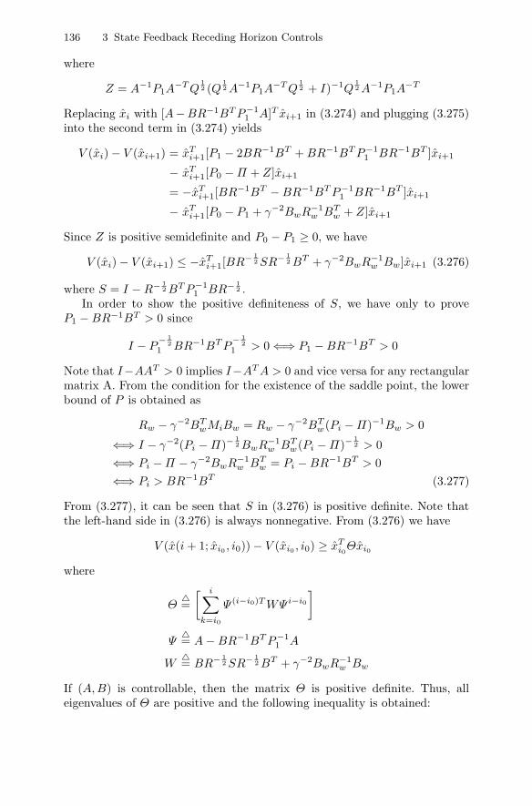
136 3 State Feedback Receding Horizon Controls

where

Z = A−1P1A−T Q

12 (Q

12 A−1P1A

−T Q12 + I)−1Q

12 A−1P1A

−T

Replacing xi with [A−BR−1BT P−11 A]T xi+1 in (3.274) and plugging (3.275)

into the second term in (3.274) yields

V (xi) − V (xi+1) = xTi+1[P1 − 2BR−1BT + BR−1BT P−1

1 BR−1BT ]xi+1

− xTi+1[P0 − Π + Z]xi+1

= −xTi+1[BR−1BT − BR−1BT P−1

1 BR−1BT ]xi+1

− xTi+1[P0 − P1 + γ−2BwR−1

w BTw + Z]xi+1

Since Z is positive semidefinite and P0 − P1 ≥ 0, we have

V (xi) − V (xi+1) ≤ −xTi+1[BR− 1

2 SR− 12 BT + γ−2BwR−1

w Bw]xi+1 (3.276)

where S = I − R− 12 BT P−1

1 BR− 12 .

In order to show the positive definiteness of S, we have only to proveP1 − BR−1BT > 0 since

I − P− 1

21 BR−1BT P

− 12

1 > 0 ⇐⇒ P1 − BR−1BT > 0

Note that I−AAT > 0 implies I−AT A > 0 and vice versa for any rectangularmatrix A. From the condition for the existence of the saddle point, the lowerbound of P is obtained as

Rw − γ−2BTwMiBw = Rw − γ−2BT

w(Pi − Π)−1Bw > 0

⇐⇒ I − γ−2(Pi − Π)−12 BwR−1

w BTw(Pi − Π)−

12 > 0

⇐⇒ Pi − Π − γ−2BwR−1w BT

w = Pi − BR−1BT > 0⇐⇒ Pi > BR−1BT (3.277)

From (3.277), it can be seen that S in (3.276) is positive definite. Note thatthe left-hand side in (3.276) is always nonnegative. From (3.276) we have

V (x(i + 1; xi0 , i0)) − V (xi0 , i0) ≥ xTi0Θxi0

where

Θ=[ i∑

k=i0

Ψ (i−i0)T WΨ i−i0

]Ψ

= A − BR−1BT P−1

1 A

W= BR− 1

2 SR− 12 BT + γ−2BwR−1

w Bw

If (A,B) is controllable, then the matrix Θ is positive definite. Thus, alleigenvalues of Θ are positive and the following inequality is obtained:

3.4 Receding Horizon Control Based on Minimax Criteria 137

V (x(i + 1; xi0 , i0)) − V (xi0) ≥ λmin(Θ)‖xi0‖ (3.278)

This implies that the closed-loop system (3.216) is exponentially increasing,i.e. the closed-loop system (3.216) with (3.270) is exponentially decreasing.This completes the proof.

In Theorem 3.20, Q can be zero. If Q becomes zero, then P1 can be ex-pressed as the following closed form:

P1 =i+N∑

j=i+1

Aj−i−1ΠA(j−i−1)T + ANPfATN (3.279)

where A is nonsingular.It is noted that Pf satisfying (3.271) is equivalent to Qf satisfying (3.243)

in the relation of Pf = Q−1f +Π. Replacing Pf with Q−1

f +Π in (3.271) yieldsthe following inequality:

Q−1f + Π ≤ A−1[Q−1

f + BR−1BT + A−T QA−1]−1A−T + Π

= [AT (Q−1f + BR−1BT )−1A + Q]−1 + Π

Finally, we have

Qf ≥ AT (Q−1f + Π)−1A + Q (3.280)

Therefore, if Qf satisfies (3.280), Pf also satisfies (3.271).

Theorem 3.21. Assume that the pair (A,B) is controllable and A is nonsin-gular.

(1) If Mi+1 ≥ Mi > 0 for some i, then the system (3.216) with the recedinghorizon H∞ control (3.222) is asymptotically stable for 1 ≤ N < ∞.

(2) For Qf > 0 satisfies (3.243) for some H, then the system (3.216) with theRH H∞ control (3.222) is asymptotically stable for 1 ≤ N < ∞.

Proof. The first part is proved as follows. Mi+1 ≥ Mi > 0 implies 0 < M−1i+1 ≤

M−1i , from which we have 0 < Pi+1 ≤ Pi satisfying the inequality (3.271).

Thus, the control (3.265) is equivalent to the control (3.222). The second partis proved as follows: inequalities Ki+1 ≥ Ki > 0 are satisfied for Ki generatedfrom Qf > 0 satisfying (3.234) for some H. Thus, the second result can beseen from the first one. This completes the proof.

It is noted that (3.280) is equivalent to (3.247), as mentioned before.

138 3 State Feedback Receding Horizon Controls

3.4.4 Additional Properties

Now, we will show that the stabilizing receding horizon controllers guaranteethe H∞ norm bound of the closed-loop system.

Theorem 3.22. Under the assumptions given in Theorem 3.18, the H∞ normbound of the closed-loop system (3.216) with (3.222) is guaranteed.

Proof. Consider the difference of the optimal cost between the time i andi + 1:

J∗(i + 1, i + N + 1) − J∗(i, i + N)

=i+N∑

j=i+1

[xT

j Qxj + uTj Ruj − γ2wT

j Rwwj

]+xT

i+N+1Qfxi+N+1

−i+N−1∑

j=i

[xT

j Qxj + uTj Ruj − γ2wT

j Rwwj

]−xT

i+NQfxi+N (3.281)

Note that the optimal control and the worst-case disturbance on the horizonare time-invariant with respect to the moving horizon.

Applying the state feedback control ui+N = Hxi+N at time i + N yieldsthe following inequality:

J∗(i + 1, i + N + 1) − J∗(i, i + N) ≤ −xTi Qxi − uT

i Rui + γ−2wTi Rwwi

+[

wi+N

xi+N

]T

Π

[wi+N

xi+N

](3.282)

where

Π=[−γ2Rw + BT

wQfBw BTwQf (A + BH)

(A + BH)T QfBw (A + BH)T Qf (A + BH) − Qf + Q + HT RH

]From the cost monotonicity condition, Π is guaranteed to be positive semidef-inite. The proof is left as an exercise. Taking the summation on both sides of(3.282) from i = 0 to ∞ and using the positiveness of Π, we have

J∗(0, N) − J∗(∞,∞ + N) =∞∑

i=0

[J∗(i, i + N) − J∗(i + 1, i + N + 1)]

≥∞∑

i=0

[xTi Qxi + uT

i Rui − γ2wTi Rwwi]

From the assumption x0 = 0, J∗(0, N) = 0. The saddle-point optimal costis guaranteed to be nonnegative, i.e. J∗(∞,∞ + N) ≥ 0. Therefore, it isguaranteed that

3.5 Receding Horizon Control via Linear Matrix Inequality Forms 139

∞∑i=0

[xTi Qxi + uT

i Rui − γ2wTi Rwwi] ≤ 0

which implies that ∑∞i=0[x

Ti Qxi + uT

i Rui]∑∞i=0 wT

i Rwwi≤ γ2

This completes the proof.

In the same way, under the assumptions given in Theorem 3.20, the H∞norm bound of the closed-loop system (3.216) with (3.222) is guaranteed withM1 replaced by [P1 − Π]−1. The inverse matrices exist for N ≥ lc + 1 sincePif−i − Π = [AT P−1

if−i−1A + Q]−1.

Example 3.3

In this example, the H∞ RHC is compared with the LQ RHC through sim-ulation. The target model and the reference signal are the same as those ofExample 3.1. except that Bw is given by

Bw =[

0.016 0.01 0.008 00.002 0.009 0 0.0005

]T

(3.283)

For simulation, disturbances coming into the system are generated so thatthey become worst on the receding horizon. γ2 is taken as 1.5.

As can be seen in Figure 3.10, the trajectory for the H∞ RHC is lessdeviated from the reference signal than that for the LQ RHC.

The MATLAB functions used for simulation are given in Appendix F.

3.5 Receding Horizon Control via Linear MatrixInequality Forms

3.5.1 Computation of Cost Monotonicity Condition

Receding Horizon Linear Quadratic Control

It looks difficult to find H and Qf that satisfy the cost monotonicity con-dition (3.73). However, this can be easily computed using LMI.

Pre- and post-multiplying on both sides of (3.73) by Q−1f , we obtain

X ≥ XQX + XHT RHX + (AX − BHX)T X−1(AX − BHX) (3.284)

where X = Q−1f . Using Schur’s complement, the inequality (3.284) is con-

verted into the following:

140 3 State Feedback Receding Horizon Controls

−0.2 0 0.2 0.4 0.6 0.8 1 1.2−0.2

0

0.2

0.4

0.6

0.8

1

1.2

ReferenceLQ RHTCH infinity RHTC

Fig. 3.10. Comparison between LQ RHTC and H∞ RHTC

X − XQX − Y T RY − (AX − BY )T X−1(AX − BY ) ≥ 0[X − XQX − Y T RY (AX − BY )T

AX − BY X

]≥ 0 (3.285)

where Y = HX. Partitioning the left side of (3.285) into two parts, we have[X (AX − BY )T

AX − BY X

]−[

XQX − Y T RY 00 0

]≥ 0 (3.286)

In order to use Schur’s complement, the second block matrix is decomposedas[

X (AX − BY )T

AX − BY X

]−[

Q12 X 0

R12 Y 0

]T [I 00 I

]−1 [Q

12 X 0

R12 Y 0

]≥ 0 (3.287)

Finally, we can obtain the LMI form as⎡⎢⎢⎣X (AX − BY )T (Q

12 X)T (R

12 Y )T

AX − BY X 0 0Q

12 X 0 I 0

R12 Y 0 0 I

⎤⎥⎥⎦ ≥ 0 (3.288)

Once X and Y are found, Qf and H = Y X−1 can be known.

Example 3.4

For the following systems and the performance criterion:

3.5 Receding Horizon Control via Linear Matrix Inequality Forms 141

xk+1 =[

0.6831 0.03530.0928 0.6124

]xk +

[0.6085 0.0158

]uk (3.289)

J(xk, k, k + N) =N−1∑i=0

[xT

k+ixk+i + 3u2k+i

]+xT

k+NQfxk+N (3.290)

The MATLAB code for finding Qf satisfying the LMI (3.288) is given inAppendix F. By using this MATLAB program, we have one possible finalweighting matrix for the cost monotonicity

Qf =[

0.4205 −0.0136−0.0136 0.4289

](3.291)

Similar to (3.73), the cost monotonicity condition (3.85) can be representedas an LMI form. First, in order to obtain an LMI form, the inequality (3.85)is converted into the following:

Qf − AT Qf [I + BR−1BT Qf ]−1A − Q ≥ 0 (3.292)[Qf − Q AT

A Q−1f + BR−1BT

]≥ 0 (3.293)

Pre- and post-multiplying on both sides of (3.293) by some positive definitematrices, we obtain[

Q−1f 00 I

]T [Qf − Q AT

A Q−1f + BR−1BT

] [Q−1

f 00 I

]≥ 0 (3.294)[

X − XQX XAT

AX X + BR−1BT

]≥ 0 (3.295)

where Q−1f = X

Partition the left side of (3.295) into two parts, we have[X XAT

AX X + BR−1BT

]−[

XQX 00 0

]≥ 0 (3.296)

In order to use Schur’s complement, the second block matrix is decomposedas [

X (AX + BY )T

AX + BY X

]−[

Q12 X 00 0

]T [I 00 I

]−1 [Q

12 X 00 0

]≥ 0 (3.297)

Finally, we can obtain the LMI form as⎡⎢⎢⎣X XAT (Q

12 X)T 0

AX X + BR−1BT 0 0Q

12 X 0 I 00 0 0 I

⎤⎥⎥⎦ ≥ 0 (3.298)

142 3 State Feedback Receding Horizon Controls

Once X is obtained, Qf is given by X−1.The cost monotonicity condition (3.98) in Theorem 3.4 can be easily ob-

tained by changing the direction of the inequality of (3.298):⎡⎢⎢⎣X XAT (Q

12 X)T 0

AX X + BR−1BT 0 0Q

12 X 0 I 00 0 0 I

⎤⎥⎥⎦ ≤ 0 (3.299)

In the following section, stabilizing receding horizon controls will be obtainedby LMIs.

Receding Horizon H∞ Control

The cost monotonicity condition (3.234) can be written[ΓI

]T [Rw − BT

wQfBw BTwQf (A − BH)

(A − BH)T QfBw Φ

] [ΓI

]≥ 0 (3.300)

where

Φ = Qf − Q − HT RH − (A − BH)T Qf (A − BH) (3.301)

From (3.300), it can be seen that we have only to find Qf such that[Rw − BT

wQfBw BTwQf (A − BH)

(A − BH)T QfBw Φ

]≥ 0 (3.302)

where we have[Rw 00 Qf − Q − HT RH

]−[

BTw

(A − BH)T

]Qf

[BT

w

(A − BH)T

]T

≥ 0 (3.303)

By using Schur’s complement, we can obtain the following matrix inequality:⎡⎣Rw 0 BTw

0 Qf − Q − HT RH (A − BH)T

Bw (A − BH) Q−1f

⎤⎦ ≥ 0 (3.304)

Multiplying both sides of (3.304) by the matrix diagI,Q−1f , I yields⎡⎣Rw 0 BT

w

0 X − XQX − XHT RHX X(A − BH)T

Bw (A − BH)X X

⎤⎦ ≥ 0 (3.305)

where Q−1f = X. Since the matrix in (3.305) is decomposed as

3.5 Receding Horizon Control via Linear Matrix Inequality Forms 143⎡⎣Rw 0 BTw

0 X (AX − BY )T

Bw AX − BY X

⎤⎦−

⎡⎣ 0 0XQ

12 Y R

12

0 0

⎤⎦⎡⎣ 0 0XQ

12 Y R

12

0 0

⎤⎦T

we have ⎡⎢⎢⎢⎢⎣Rw 0 BT

w 0 00 X (AX − BY )T XQ

12 Y R

12

Bw AX − BY X 0 00 Q

12 X 0 I 0

0 R12 Y T 0 0 I

⎤⎥⎥⎥⎥⎦ ≥ 0 (3.306)

where Y = HX.

3.5.2 Receding Horizon Linear Quadratic Control via Batch andLinear Matrix Inequality Forms

In the previous section, the receding horizon LQ control was obtained ana-lytically in a closed form, and thus it can be easily computed. Here, how toachieve the receding horizon LQ control via an LMI is discussed, which willbe utilized later in constrained systems.

Free Terminal Cost

The state equation in (3.3) can be written as

Xk = Fxk + HUk (3.307)

Uk =

⎡⎢⎢⎢⎣uk

uk+1

...uk+N−1

⎤⎥⎥⎥⎦ , Xk =

⎡⎢⎢⎢⎣xk

xk+1

...xk+N−1

⎤⎥⎥⎥⎦ , F =

⎡⎢⎢⎢⎣IA...

AN−1

⎤⎥⎥⎥⎦ (3.308)

H =

⎡⎢⎢⎢⎢⎢⎣0 0 0 · · · 0B 0 0 · · · 0

AB B 0 · · · 0...

.... . .

......

AN−2B AN−3B · · · B 0

⎤⎥⎥⎥⎥⎥⎦ (3.309)

The terminal state is given by

xk+N = ANxk + BUk (3.310)

whereB =

[AN−1B AN−2B · · · B

](3.311)

144 3 State Feedback Receding Horizon Controls

Let us define

QN = diagN︷ ︸︸ ︷

Q, · · · , Q, RN = diagN︷ ︸︸ ︷

R, · · · , R (3.312)

Then, the cost function (3.22) can be rewritten by

J(xk, Uk) = [Xk − Xrk ]T QN [Xk − Xr

k ] + UTk RNUk

+ (xk+N − xrk+N )T Qf (xk+N − xr

k+N )

where

Xrk =

⎡⎢⎢⎢⎣xr

k

xrk+1...

xrk+N−1

⎤⎥⎥⎥⎦From (3.307) and (3.310), the above can be represented by

J(xk, Uk) = [Fxk + HUk − Xrk ]T QN [Fxk + HUk − Xr

k ] + UTk RNUk

+ [ANxk + BUk − xrk+N ]T Qf [ANxk + BUk − xr

k+N ]

= UTk [HT QNH + RN ]Uk + 2[Fxk − Xr

k ]T QNHUk

+ [Fxk − Xrk ]T QN [Fxk − Xr

k ]+ [ANxk + BUk − xr

k+N ]T Qf [ANxk + BUk − xrk+N ]

= UTk WUk + wT Uk + [Fxk − Xr

k ]T QN [Fxk − Xrk ]

+ [ANxk + BUk − xrk+N ]T Qf [ANxk + BUk − xr

k+N ] (3.313)

where W = HT QNH + RN and w = 2HT QTN [Fxk − Xr

k ]. The optimal inputcan be obtained by taking ∂J(xk,Uk)

∂Uk. Thus we have

Uk = −[W + BT Qf B]−1[w + BT Qf (ANxk − xrk+N )]

= −[W + BT Qf B]−1[HT QN (Fxk − Xrk)

+ BT Qf (ANxk − xrk+N )] (3.314)

The RHC can be obtained as

uk =[1, 0, · · · , 0

]U∗

k (3.315)

In order to obtain an LMI form, we decompose the cost function (3.313) intotwo parts

J(xk, Uk) = J1(xk, Uk) + J2(xk, Uk)

where

J1(xk, Uk) = UTk WUk + wT Uk + [Fxk − Xr

k ]T QN [Fxk − Xrk ]

J2(xk, Uk) = (ANxk + BUk − xrk+N )T Qf (ANxk + BUk − xr

k+N )

3.5 Receding Horizon Control via Linear Matrix Inequality Forms 145

Assume that

UTk WUk + wT Uk + [Fxk − Xr

k ]T QN [Fxk − Xrk ] ≤ γ1 (3.316)

(ANxk + BUk − xrk+N )T Qf (ANxk + BUk − xr

k+N ) ≤ γ2 (3.317)

Note thatJ(xk, Uk) ≤ γ1 + γ2 (3.318)

From Schur’s complement, (3.316) and (3.317) are equivalent to[γ1 − wT Uk − [Fxk − Xr

k ]T QN [Fxk − Xrk ] UT

k

Uk W−1

]≥ 0 (3.319)

and [γ2 [ANxk + BUk − xr

k+N ]T[ANxk + BUk − xr

k+N

]Q−1

f

]≥ 0 (3.320)

respectively. Finally, the optimal solution U ∗k can be obtained by an LMI

problem as follows:

minUk

γ1 + γ2 subject to (3.319) and (3.320)

Therefore, the RHC in a batch form is obtained by

uk =[1, 0, · · · , 0

]U∗

k (3.321)

Terminal Equality Constraint

The optimal control (3.314) can be rewritten by

Uk = −[[

HB

]T [QN 00 Qf

] [HB

]+ RN

]−1 [HB

]T [QN 00 Qf

]×[[

FAN

]xk −

[Xr

k

xrk+N

]]= −R−1

N

[[HB

]T [QN 00 Qf

] [HB

]R−1

N + I

]−1 [HB

]T [QN 00 Qf

]×[[

FAN

]xk −

[Xr

k

xrk+N

]](3.322)

We define

H =[

HB

]F =

[F

AN

]Xr

k =[

Xrk

xrk+N

](3.323)

Then, using the formula (I + AB)−1A = A(I + BA)−1, we have

146 3 State Feedback Receding Horizon Controls

Uk = −R−1N HT [QN HR−1

N HT + I]−1QN [F − I][

xk

Xrk

]= −R−1

N HT [QN2HR−1N HT + Q−1

N1]−1QN2[F − I]

[xk

Xrk

](3.324)

where

QN =[

QN 00 Qf

]=[

I 00 Qf

] [QN 00 I

]= QN1QN2 (3.325)

For terminal equality constraint, we take Qf = ∞I (Q−1f = 0). So Uk is

given as (3.324) with Q−1N1 replaced by

[I 00 0

].

We introduce an LMI-based solution. In a fixed terminal case, (3.317) isnot used. Instead, the condition ANxk + BUk = xr

k+N should be met. Thus,we need an equality condition together with an LMI. In order to removethe equality representation, we parameterize Uk in terms of known variablesaccording to Theorem A.3. We can set Uk as

Uk = −B−1(ANxk − xrk+N ) + MUk (3.326)

where B−1 is the right inverse of B and columns of M are orthogonal to eachother, spanning the null space of B.

From (3.316) we have

J(xk, Uk) = UTk WUk + wT Uk + [Fxk − Xr

k ]T QN [Fxk − Xrk ]

= (−B−1(ANxk − xrk+N ) + MUk)T W (−B−1(ANxk − xr

k+N )

+ MUk) + wT (−B−1(ANxk − xrk+N ) + MUk) + [Fxk − Xr

k ]T QN

× [Fxk − Xrk ]

= UTk V1Uk + V2Uk + V3

where

V1 = MT WM

V2 = −2(ANxk − xrk+N )T B−T WM + wT M

V3 = (ANxk − xrk+N )T B−T WB−1(ANxk − xr

k+N )

+ [Fxk − Xrk ]T QN [Fxk − Xr

k ] − wT B−1(ANxk − xrk+N )

The optimal input can be obtained by taking ∂J(xk,Uk)

∂Uk. Thus we have

Uk = −V−11 VT

2

The RHC in a batch form can be obtained as in (3.315). The optimal con-trol for the fixed terminal case can be obtained from the following inequality:

J(xk, Uk) = UTk V1Uk + V2Uk + V3 ≤ γ1

3.5 Receding Horizon Control via Linear Matrix Inequality Forms 147

which can be transformed into the following LMI:

min γ1[γ1 − V2Uk − V3 −UT

k V121

−V121 Uk I

]≥ 0

where Uk is obtained. Uk is computed from this according to (3.326). Whatremains to do is just to pick up the first one among Uk as in (3.321).

GPC for the CARIMA model (3.194) can be obtained in a batch formsimilar to that presented above. From the state-space model (3.200), we have

yk+j = CAjxk +j−1∑i=0

CAj−i−1Buk+i (3.327)

The performance index (3.204) can be represented by

J = [Y rk − V xk − WUk]T Q [Y r

k − V xk − WUk] + UTk RUk

+[Y r

k+Nc− Vfxk − WfUk

]TQf

[Y r

k+Nc− Vfxk − WfUk

](3.328)

where

Y rk =

⎡⎢⎣ yrk+1...

yrk+Nc

⎤⎥⎦ , V =

⎡⎢⎣ CA...

CANc

⎤⎥⎦ , Uk =

⎡⎢⎣ uk

...uk+Nc−1

⎤⎥⎦

Y rk+Nc

=

⎡⎢⎣ yrk+Nc+1

...yr

k+Np

⎤⎥⎦ , Vf =

⎡⎢⎣ CANc+1

...CANp

⎤⎥⎦ , W =

⎡⎢⎣ CB · · · 0...

. . ....

CANc−1B · · · CB

⎤⎥⎦

Wf =

⎡⎢⎣ CANcB · · · CAB...

. . ....

CANp−1B · · · CANp−NcB

⎤⎥⎦ , R =[diag(

Nc︷ ︸︸ ︷r r · · · r)

]

Qf =[diag(

Np−Nc︷ ︸︸ ︷qf qf · · · qf )

], Q =

[diag(

Nc︷ ︸︸ ︷q q · · · q)

].

Using

∂J

∂Uk= 0

we can obtain

Uk =[WT QW + WT

f QfWf + R]−1

WT Q [Y rk − V xk]

+WTf Qf

[Y r

k+Nc− Vfxk

]

148 3 State Feedback Receding Horizon Controls

Therefore, uk is given by

uk =[I 0 · · · 0

] [WT QW + WT

f QfWf + R]−1

WT Q [Y rk − V xk]

+WTf Qf

[Y r

k+Nc− Vfxk

](3.329)

3.5.3 Receding Horizon H∞ Control via Batch and Linear MatrixInequality Forms

In the previous section, the receding horizon H∞ control was obtained ana-lytically in a closed form and thus it can be easily computed. Here, how toachieve the receding horizon H∞ control via LMI is discussed.

The state equation (3.9) can be represented by

Xk = Fxk + HUk + HwWk (3.330)

where Hw is given by

Hw =

⎡⎢⎢⎢⎢⎢⎣0 0 0 · · · 0G 0 0 · · · 0

AG G 0 · · · 0...

.... . .

......

AN−2G AN−3G · · · G 0

⎤⎥⎥⎥⎥⎥⎦ (3.331)

and Uk, F , Xk, and H are defined in (3.308) and (3.309).The H∞ performance criterion can be written in terms of the augmented

matrix as

J(xk, Uk,Wk) = [Fxk + HUk + HwWk − Xrk ]T QN [Fxk + HUk + HwWk

− Xrk ] + [ANxk + BUk + GWk − xr

k+N ]T Qf [ANxk + BUk

+ GWk − xrk+N ] + UT

k RNUk − γ2WTk Wk

Representing J(xk, Uk,Wk) in quadratic form with respect to Wk yields thefollowing equation:

J(xk, Uk,Wk) = WTk V1Wk + 2WT

k V2 + [Fxk + HUk − Xrk ]T QN [Fxk + HUk

− Xrk ] + UT

k RNUk + [ANxk + BUk − xrk+N ]T Qf [ANxk + BUk

− xrk+N ]

= [V1Wk + V2]TV−11 [V1Wk + V2] − VT

2 V−11 V2 + UT

k RNUk

+ [Fxk + HUk − Xrk ]T QN [Fxk + HUk − Xr

k ]+ [ANxk + BUk − xr

k+N ]T Qf [ANxk + BUk − xrk+N ]

= [V1Wk + V2]TV−11 [V1Wk + V2] + UT

k P1Uk + 2UTk P2

+ P3 (3.332)

3.5 Receding Horizon Control via Linear Matrix Inequality Forms 149

where

V1= −γ2I + GT Qf G + HT

w QNHw (3.333)

V2= HT

w QTN [Fxk + HUk − Xr

k ] + GT QTf [ANxk + BUk − xr

k+N ] (3.334)

P1= −(HT

w QTNH + GT QT

f B)TV−11 (HT

w QTNH + GT QT

f B)

+ HT QNH + RN + BT Qf B (3.335)

P2= −(HT

w QTNH + GT QT

f B)TV−11 (HT

w QTN (Fxk − Xr

k)

+ GT QTf (ANxk − xr

k+N )) + HT QNFxk + BT QfANxk (3.336)

and P3 is a constant that is independent of Uk and Wk.In order that the solution to the saddle point exists, V1 must be negative.

Thus, we have

−γ2I + GT Qf G + HTw QNHw < 0

In order to maximize (3.332) with respect to Wk, we have only to maximize

[V1Wk + V2]TV−11 [V1Wk + V2] (3.337)

to obtainWk = −V−1

1 V2 (3.338)

If we put (3.338) into (3.332), (3.332) can be represented by

J(xk, Uk,Wk) = UTk P1Uk + 2UT

k P2 + P3 (3.339)

Then the optimal input can be obtained by taking ∂J(xk,Uk,Wk)∂Uk

. Thus we have

Uk = −P−11 P2

Now we can introduce an LMI form for the receding horizon H∞ control.In order to maximize (3.332) with respect to Wk, we have only to minimize

−[V1Wk + V2]TV−11 [V1Wk + V2] (3.340)

Then we try to minimize (3.339). It follows finally that we have the followingLMI:

minUk,Wk

r1 + r2 (3.341)[r1 − PT

2 Uk UTk

Uk P−11

]≥ 0[

r2 (V1Wk + V2)T

(V1Wk + V2) −V1

]≥ 0

The stabilizing RH H∞ control can be obtained by solving the semidefiniteprogram (3.306) and (3.341) where Qf = X−1. What remains to do is just topick up the first one among Uk as in (3.321).

An LMI representation in this section would be useful for constrainedsystems.

150 3 State Feedback Receding Horizon Controls

3.6 References

In order to explain the receding horizon concept, the predictor form and thereference predictive form are introduced first in Section 3.2.1 of this chapter.

The primitive form of the RH control was given in [Kle70] [Kle74], whereonly input energy with fixed terminal constraint is concerned without theexplicit receding horizon concept. The general form of the RHC was firstgiven with receding horizon concepts in [KP77a], where state weighting isconsidered. The RHTC presented in Section 3.3.1 is similar to that in [KB89].

With a terminal equality constraint which corresponds to the infinite ter-minal weighting matrix, the closed-loop stability of the RHC was first provedin a primitive form [Kle70] and in a general form [KP77a]. There are alsosome other results in [Kle74] [KP78] [AM80] [NS97].

The terminal equality constraint in Theorem 3.1 is a well-known result.Since the terminal equality constraint is somewhat strong, finite terminal

weighting matrices for the free terminal cost have been investigated in [Yaz84][BGP85] [KB89] [PBG88] [BGW90] [DC93] [NP97] [LKC98]. The monotoneproperty of the Ricatti equation is used for the stability [KP77a]. Later, themonotone property of the optimal cost was introduced not only for linear, butalso for nonlinear systems. At first, the cost monotonicity condition was usedfor the terminal equality constraint [KRC92] [SC94][RM93][KBM96] [LKL99].The cost monotonicity condition for free terminal cost in Theorem 3.2 is firstgiven in [LKC98]. The general proof of Theorem 3.2 is a discrete version of[KK00]. The inequality (3.84) is a special case of (3.73) and is partly studied in[KB89] [BGW90]. The terminal equality constraint comes historically beforethe free terminal cost. The inequality between the terminal weighting matrixand the steady-state Riccati solution in Proposition 3.3 appeared first in thisbook.

The opposite direction of the cost monotonicity in Theorem 3.4 is firstintroduced for discrete systems in this book. It is shown in [BGW90] thatonce the monotonicity of the Riccati equation holds at a certain point it holdsfor all subsequent times as in Theorem 3.5.

The stability of RHCs in Theorems 3.6 and 3.7 is first introduced in[LKC98] and the general proofs of these theorems in this book are discreteversions of [KK00].

The stability of the RHC in the case of the terminal equality constraint inTheorem 3.7 is derived by using Theorems 3.1 and 3.6.

A stabilizing control in Theorem 3.9 is first introduced in [LKC98] withouta proof, and thus a proof is included in this book by using Lyapunov theory.

The observability in Theorems 3.6 and 3.9 can be weakened with de-tectability, similar to that in [KK00].

The results on Theorems 3.10 and 3.11 appear first in this book and areextensions of [KP77a]. For time-invariant systems, the controllability in The-orems 3.10 and 3.11 can be weakened with stabilizability, as shown in [RM93]

3.7 Problems 151

and [KP77a]. The closed-loop stability of the RHC via FARE appears in[PBG88, BGW90]

The lower bound of the horizon size stabilizing the system in Theorem3.12 appeared in [JHK04].

The RH LQ control with a prescribed degree of stability appeared in[KP77b] for continuous-time systems. In Section 3.3.5 of this book, slightmodifications are made to obtain it for discrete-time systems.

The upper and lower bounds of the performance criteria in Theorems3.13 and 3.14 are discrete versions of the result [KBK83] for continuous-timesystems.

It was shown in [KBK83] that the RH LQ control stabilizes the system fora sufficiently large horizon size irrespective of the final weighting matrix.

The RH H∞ control presented in Section 3.4.1 is a discrete version of thework by [KYK01]. The cost monotonicity condition of the RH H∞ control inTheorems 3.15, 3.16, and 3.17 is a discrete version of the work by [KYK01].The stability of the RH H∞ control in Theorems 3.18 and 3.19 also appeared in[KYK01]. The free terminal cost in the above theorems was proposed in [LG94][LKL99]. The relation between the free terminal cost and the monotonicity ofthe saddle point value was fully discussed in [KYK01].

The RH H∞ control without requiring the observability of (A,Q12 ), as in

Theorems 3.20 and 3.21, is first discussed in this book in parallel with the RHLQ control.

The guaranteed H∞ norm of the H∞ RHC in Theorem 3.22 is first givenin this book for discrete-time systems by a modification of the result oncontinuous-time systems in [KYK01].

In [LKC98], how to obtain the receding horizon control and a final weight-ing matrix satisfying the cost monotonicity condition was discussed by usingLMIs. Sections 3.5.1 and 3.5.2 are mostly based on [LKC98].

The RHLQC with the equality constraint and the cost monotonicity con-dition for the H∞ RHC in an LMI form appear first in Sections 3.5.2 and3.5.3 of this book respectively.

3.7 Problems

3.1. Referring to Problem 2.6, make simulations for three kinds of planningbased on Table 1.1. α, γ, β, u are set to 0.8, 1.3, 10, and 1 respectively. Forlong-term planning, use N = 100. For periodic and short-term planning, useN = 5 and a simulation time of 100.

3.2. Derive a cost monotonicity condition for the following performance cri-terion for the system (3.1):

J(xi0 , u·) =if−1∑i=i0

[xi

ui

]T [Q SST R

] [xi

ui

]+ xT

ifQfxif

152 3 State Feedback Receding Horizon Controls

3.3. (1) If Qf satisfies a cost monotonicity condition, show that the RHCwith this Qf can be an infinite horizon optimal control (2.107) with somenonnegative symmetric Q and some positive definite R.

(2) Verify that the RHC with the equality constraint has the property thatit is an infinite horizon optimal control (2.107) associated with some non-negative symmetric Q and some positive definite R.

3.4. Consider the cost monotonicity condition (3.73).

(1) Show that the condition (3.73) can be represented as

Qf ≥ minH

Q + HT RH + (A − BH)T Qf (A − BH)

(3.342)

(2) Choose H so that the right side of (3.342) is minimized.

3.5. Consider a discrete-time system as

xi+1 =[

0 01 0

]xi +

[10

]ui (3.343)

(1) Find an RHC for the following performance criterion:

xTk+1|k

[1 22 6

]xk+1|k + u2

k|k (3.344)

where the horizon size is 1. Check the stability.(2) Find an RHC for the following performance criterion:

1∑j=0

xTk+j|k

[1 22 6

]xk+j|k + u2

k+j|k + xTk+2|k

[1 00 0

]xk+2|k (3.345)

where the horizon size is 2. Check the stability.(3) In the problem (b), introduce the final weighting matrix as

1∑j=0

xTk+j|k

[1 22 6

]xk+j|k + u2

k+j|k + xTk+2|kQfxk+2|k (3.346)

and find Qf such that the system is stabilized.

3.6. Suppose that Qf is positive definite and the system matrix A is nonsin-gular.

(1) Prove that the solution to Riccati Equation (3.49) is positive definite.(2) Let V (xi) = xT

i A−1(K−11 + BR−1BT )A−T xi, where K1 is obtained from

the Riccati equation starting from KN = Qf , then show that the systemcan be stabilized. (Hint: use Lasalle’s theorem and the fact that if A isHurwitz, then so is AT .)

3.7 Problems 153

Remark: in the above problem, the observability of (A,Q12 ) is not required.

3.7. Prove the stability of the RHC (3.49) by using Lyapunov theory.

(1) Show that K1 defined in (3.47) satisfies

K1 ≥ (A − BL1)T K1(A − BL1) + LT1 RL1 + Q (3.347)

starting from KN = Qf satisfying (3.73) and L1 = [R+BT K1B]−1BT K1A.(2) Show that xT

i K1xi in (3.347) can be a Lyapunov function. Additionally,show the stability of the RHC under assumptions that (A,B) and (A,Q

12 )

are stabilizable and observable respectively.

3.8. Consider the FARE (3.122). Suppose that (A,B) is stabilizable, Q ≥ 0,and (A, Q

12 ) is observable. If Ki0+2 − 2Ki0+1 + Ki0 ≤ 0 for some i0, then the

system with the RHC (3.55) is stable for any N ≥ i0.

3.9. ∗ Denote the control horizon and the prediction horizon as Nc and Np

respectively. This book introduces various RHC design methods in the caseof N = Nc = Np. When we use different control and prediction horizons(Nc = Np):

(1) discuss the effect on the computational burden.(2) discuss the effect on the optimal performance.

3.10. In this chapter, ‖A‖ρ,ε is introduced.

(1) Take an example that does not satisfy the following inequality

ρ(AB) ≤ ρ(A)ρ(B)

where ρ(A) is the spectral radius.(2) Show that there always exists a matrix norm ‖A‖ρ,ε such that

ρ(A) ≤ ‖A‖ρ,ε ≤ ρ(A) + ε (3.348)

for any ε > 0.(3) Disprove that ρ(A) ≤ 1 implies ‖A‖2 ≤ 1

3.11. Let Ki be the solution to the difference Riccati equation (2.45) and Li

its corresponding state feedback gain (2.57). K and L are the steady-statevalues of Ki and Li.(1) Show that

Li+1 − L = −R−1o,i+1B

TKi+1Ac (3.349)

Ac,i+1 = A − BLi+1 = (I − BR−1o,i+1B

TKk+1)Ac (3.350)

where

Ro,i+1= R + BT KiB, Ki

= Ki − K, Ac

= A − BL

(2) Show that

Ki = ATc [Ki+1 −Ki+1BR−1

o,i+1BTKi+1]Ac (3.351)

154 3 State Feedback Receding Horizon Controls

3.12. Suppose that the pair (A,B) and (A,Q12 ) are controllable and observ-

able respectively.

(1) Show that the closed-loop system can be written as

xi+1 = Gixi + BR−1BT Kei+1,NAxi (3.352)

with

Gi = A − BR−1BT Ki+1,∞A (3.353)

Ki+1,i+N = [K−1i+1,i+N + BR−1BT ]−1 (3.354)

Kei+1,N = Ki+1,∞ − Ki+1,i+N (3.355)

where Ki+1,i+N is given in (3.47) and Ki+1,∞ is the steady-state solutionof (3.47).

(2) Prove that, for all x,

limN→∞

|BR−1BT Kei+1,NAx|

|x| = 0 (3.356)

(3) Show that there exists a finite horizon size N such that the RHC (3.56)stabilizes the closed-loop system.Hint. Use the following fact: suppose that xi+1 = f(xi) is asymptoticallystable and g(xi, i) satisfies the equality limi→∞

g(xi,i)xi

= 0. Then, xi+1 =f(xi) + g(xi, i) is also stable.

3.13. A state-space model is given as

xi+1 =[

2 13 4

]xi +

[23

]ui (3.357)

where

Q =[

2 00 2

], R = 2 (3.358)

(1) According to the formula (3.149), find a lower bound of the horizon sizeN that guarantees the stability irrespective of the final weighting matrixQf .

(2) Calculate a minimum horizon size stabilizing the closed-loop systems bydirect computation of the Riccati equation and closed-loop poles.

3.14. MAC used the following model:

yk =n−1∑i=0

hiuk−i

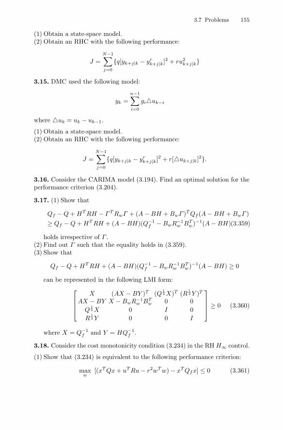
3.7 Problems 155

(1) Obtain a state-space model.(2) Obtain an RHC with the following performance:

J =N−1∑j=0

q[yk+j|k − yrk+j|k]2 + ru2

k+j|k

3.15. DMC used the following model:

yk =n−1∑i=0

giuk−i

where uk = uk − uk−1.

(1) Obtain a state-space model.(2) Obtain an RHC with the following performance:

J =N−1∑j=0

q[yk+j|k − yrk+j|k]2 + r[uk+j|k]2.

3.16. Consider the CARIMA model (3.194). Find an optimal solution for theperformance criterion (3.204).

3.17. (1) Show that

Qf − Q + HT RH − ΓT RwΓ + (A − BH + BwΓ )T Qf (A − BH + BwΓ )≥ Qf − Q + HT RH + (A − BH)(Q−1

f − BwR−1w BT

w)−1(A − BH)(3.359)

holds irrespective of Γ .(2) Find out Γ such that the equality holds in (3.359).(3) Show that

Qf − Q + HT RH + (A − BH)(Q−1f − BwR−1

w BTw)−1(A − BH) ≥ 0

can be represented in the following LMI form:⎡⎢⎢⎣X (AX − BY )T (Q

12 X)T (R

12 Y )T

AX − BY X − BwR−1w BT

w 0 0Q

12 X 0 I 0

R12 Y 0 0 I

⎤⎥⎥⎦ ≥ 0 (3.360)

where X = Q−1f and Y = HQ−1

f .

3.18. Consider the cost monotonicity condition (3.234) in the RH H∞ control.

(1) Show that (3.234) is equivalent to the following performance criterion:

maxw

[(xT Qx + uT Ru − r2wT w) − xT Qfx] ≤ 0 (3.361)

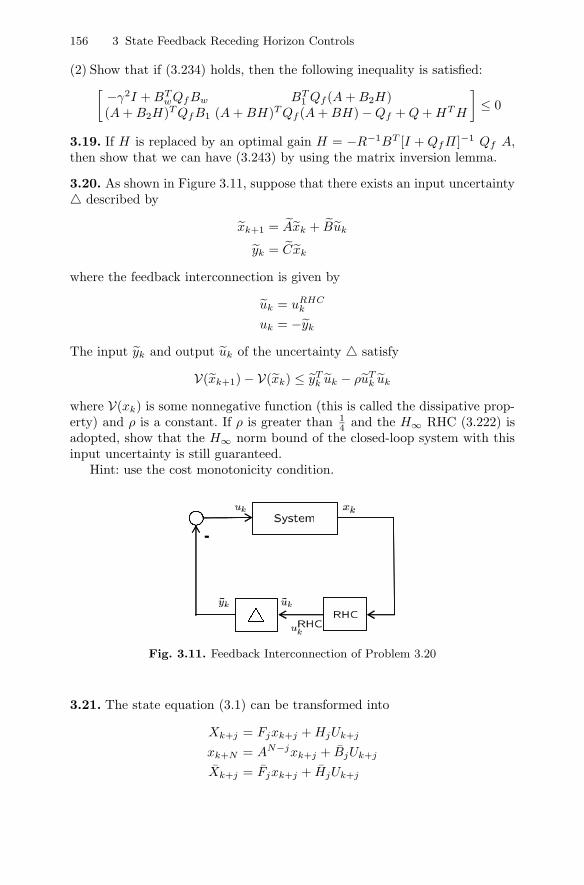
156 3 State Feedback Receding Horizon Controls

(2) Show that if (3.234) holds, then the following inequality is satisfied:[−γ2I + BT

wQfBw BT1 Qf (A + B2H)

(A + B2H)T QfB1 (A + BH)T Qf (A + BH) − Qf + Q + HT H

]≤ 0

3.19. If H is replaced by an optimal gain H = −R−1BT [I + QfΠ]−1 Qf A,then show that we can have (3.243) by using the matrix inversion lemma.

3.20. As shown in Figure 3.11, suppose that there exists an input uncertainty described by

xk+1 = Axk + Buk

yk = Cxk

where the feedback interconnection is given by

uk = uRHCk

uk = −yk

The input yk and output uk of the uncertainty satisfy

V(xk+1) − V(xk) ≤ yTk uk − ρuT

k uk

where V(xk) is some nonnegative function (this is called the dissipative prop-erty) and ρ is a constant. If ρ is greater than 1

4 and the H∞ RHC (3.222) isadopted, show that the H∞ norm bound of the closed-loop system with thisinput uncertainty is still guaranteed.

Hint: use the cost monotonicity condition.

--

Fig. 3.11. Feedback Interconnection of Problem 3.20

3.21. The state equation (3.1) can be transformed into

Xk+j = Fjxk+j + HjUk+j

xk+N = AN−jxk+j + BjUk+j

Xk+j = Fjxk+j + HjUk+j

3.7 Problems 157

where 0 ≤ j ≤ N − 1.

Uk+j =

⎡⎢⎢⎢⎣uk+j

uk+j+1

...uk+N−1

⎤⎥⎥⎥⎦ , Xk+j =

⎡⎢⎢⎢⎣xk+j

xk+j+1

...xk+N−1

⎤⎥⎥⎥⎦

Fj =

⎡⎢⎢⎢⎣IA...

AN−1−j

⎤⎥⎥⎥⎦ =[

IFj+1A

]

Hj =

⎡⎢⎢⎢⎢⎢⎣0 0 0 · · · 0B 0 0 · · · 0

AB B 0 · · · 0...

.... . .

......

AN−2−jB AN−3−jB · · · B 0

⎤⎥⎥⎥⎥⎥⎦ =[

0 0Fj+1B Hj+1

]

Bj =[AN−1−jB AN−2−jB · · · AB B

]Xk+j =

[Xk+j

xk+N

], Fj =

[Fj

AN−j

], Hj =

[Hj

Bj

](1) We define

Kj = FTj QjFj − FT

j QjHj(HTj QjHj + Rj)−1HT

j QjFj

where

Qj = diagN−j+1︷ ︸︸ ︷

Q, · · · , Q Qf, Rj = diagN−j+1︷ ︸︸ ︷

R, · · · , R.Then, show that the optimal control (3.314) can be rewritten by

Uk+j = −[HTj QjHj + Rj ]−1HT

j QjFjxk+j (3.362)

=[

−[R + BT Kj+1B]−1BT Kj+1Axk+j

−[Rj+1 + HTj+1Qj+1Hj+1]−1HT

j+1Qj+1Fj+1xk+j+1

]=[

uk+j

Uk+j+1

](2) Show that the above-defined Kj satisfies (3.47), i.e. the recursive solution

can be obtained from a batch form of solution.

3.22. Consider the GPC (3.329) for the CARIMA model (3.194).

(a) Using (3.329), obtain the GPC uk when Qf = ∞I.(b) Show that the above GPC is asymtotically stable.3.23. In Section 2.5, the optimal control Uk on the finite horizon was obtainedfrom the LMI approach. Derive an LMI for the control gain H of Uk = Hxk,not the control Uk itself.

4

Receding Horizon Filters

4.1 Introduction

In the previous chapters we have used state feedback under the assumptionthat all the state variables are available. However, this assumption may nothold in practice, since the state information may not be measurable or it maycost a lot to measure all state variables. In this case we have to use outputfeedback controls that utilize measured inputs and outputs. A state can beestimated from measured inputs and outputs. Thus, output feedback controlscan be obtained by replacing the real state in state feedback controls by theestimated state. In this chapter we shall introduce state observers, or filtersthat estimate the state from the measured inputs and outputs.

In the control area, filters can be used for the output feedback control, andin the signal processing area, filters can be used for the separation of real sig-nals from noisy signals. Therefore, the results in this chapter will be useful notonly for control, but also for signal processing. In Chapter 1, control models,control objectives, control structures, and control performance criteria werediscussed for control designs. In this chapter, signal models, filter objectives,filter structures, and filter performance criteria are introduced, as in Figure4.1, for filter designs.

Signal Models

Models, often called signal models, are mathematical description of physi-cal systems under consideration. Models are constructed from the measureddata about physical systems. The more a priori information we can incor-porate into the model, the better model we can obtain. Models fall into theseveral classes by the type of underlying mathematical equations, i.e. linearor nonlinear, state space or I/O, deterministic or stochastic, time-invariant orvarying. Undesirable elements such as disturbances, noises, and uncertaintiesof dynamics can be included in the model. In this chapter we focus on lineartime-invariant systems that are represented by state-space models with deter-ministic disturbances or stochastic noises.

160 4 Receding Horizon Filters

Filter Objectives

There can be several objectives of filter designs. Actually, the stability andthe performance even under the above undesirable elements are consideredimportant. Since it is difficult to obtain a filter under general frameworks, thefilter can be designed first for simpler models, i.e. nominal systems and thenfor general systems, i.e. uncertain systems. Thus, the goals can be categorizedinto some simpler intermediate ones, such as:

• Nominal stability. The estimation error approaches zero for signal modelswithout uncertainties.

• Nominal performance. The filter satisfies the performance criteria for sig-nal models without uncertainties.

• Robust stability. The estimation error approaches zero for signal modelswith uncertainties.

• Robust performance. The filter satisfies the performance criteria for signalmodels with uncertainties.

Filter Structure

Filters are of various forms. Filters can process the given information linearlyor nonlinearly. Linear filters are easily implemented and have less computationload than nonlinear filters.

Filters can be divided into FIR filters and IIR filters on the basis of theduration of the impulse response. Recursive IIR filters such as the conventionalKalman filters are especially popular in control areas, but they may havesome undesirable problems, such as divergences. Nonrecursive FIR filters arepopular in signal processing areas and may have some good properties, suchas the guaranteed stability.

Filters can be independent of the initial state information. There are somecases in which initial state information is not used: the initial state informationis unknown, as it often is in the real world; the measurement of the initialstate is avoided due to its cost; or the initial state can be ignored because wecan use certain approaches that do not require the initial state information.Kalman filters are implemented under the assumption that the information ofthe initial state is available. Thus, filter coefficients or gains may be dependenton the initial state, which does not make sense.

Unbiasedness has been considered to be a good property in the literaturefor a long time. Conventionally, this is checked after a filter is designed. How-ever, the unbiased property can be built in to a filter during the design phase.

Performance Criterion

The performance criteria can take many forms. An optimal filter is obtainedby minimizing or mini-maximizing a certain performance criterion. In the

4.2 Dual Infinite Impulse Response Filter Based on Minimum Criterion 161

stochastic case, the performance criterion such as a minimum variance can becast as a minimization problem. In the deterministic case, the performancecriteria such as H∞ can be posed mathematically as a mini-maximizationproblem. A least squares operation for the minimization performance crite-rion can be used for both deterministic and stochastic systems.

In this chapter we introduce either IIR or FIR filters which correspondto receding horizon controls in Chapter 3. In particular, we introduce a dualIIR filter whose gain is dual to the receding horizon control. Then we willintroduce optimal FIR filters which use the receding horizon concept for themeasured data. FIR filters are implemented each time with the finite recentmeasurement information.

For FIR filters, linearity, unbiasedness, FIR structure, and the indepen-dence of the initial state information are built in during the design phase. Inthe signal processing area, the FIR filter has been widely used for unmodelledsignals due to its many good properties, such as guaranteed stability, linearphase(zero error), robustness to temporary parameter changes and round-offerror, etc. Good properties of FIR filters for the state estimation will be in-vestigated in this chapter.

The sections with an asterisk are provided for a general system matrix A.Complex notation is required, so that this section may be skipped for a firstreading.

The organization of this chapter is as follows. In Section 4.2, dual filtersto receding horizon LQ controls are introduced with inherent properties. InSection 4.3, minimum variance FIR filters are first given for the nonsingularmatrix A for simplicity and then for the general (possibly singular) matrixA. Both batch and recursive forms are provided. In Section 4.4, dual filtersto receding horizon H∞ controls are introduced with inherent properties. InSection 4.5, minimax FIR filters, such as L2-E FIR filters and H∞ filters, areintroduced.

4.2 Dual Infinite Impulse Response Filter Based onMinimum Criterion

Consider a linear discrete-time state-space model:

xi+1 = Axi + Bui + Gwi (4.1)yi = Cxi + vi (4.2)

where xi ∈ n is the state, and ui ∈ l and yi ∈ q are the input andmeasurement respectively. At the initial time i0 of the system, the state xi0

is a random variable with a mean xi0 and a covariance Pi0 . The system noisewi ∈ p and the measurement noise vi ∈ q are zero-mean white Gaussianand mutually uncorrelated. The covariances of wi and vi are denoted by Qw

162 4 Receding Horizon Filters

Fig. 4.1. Filter components

and Rv respectively, which are assumed to be positive definite matrices. Thesenoises are uncorrelated with the initial state xi0 . (A,C) of the system (4.1)and (4.2) is assumed to be observable, so that the stable observer can beconstructed.

Before we introduce a filter for (4.1) and (4.2), we will compare the LQcontrol with the Kalman filter and investigate structural differences betweenthem. The LQ control (2.48) with a zero reference signal and a terminal timei0 + N is given by

u∗i = −[R + BT Ki+1B]−1BT Ki+1Axi (4.3)

where Riccati Equation (2.45) is given by

Ki = AT [I + Ki+1BR−1BT ]−1Ki+1A + Q (4.4)

with

Ki0+N = Qf (4.5)

Meanwhile, the receding horizon control (3.56) is given by

u∗i = −R−1BT [I + K1BR−1BT ]−1K1Axi

= −[R + BT K1B]−1BT K1Axi (4.6)

where K1 is computed from (4.4) with the terminal condition KN = Qf . Ki

in the control gain matrix in (4.3) is time-varying and K1 in the gain matrix(4.6) is fixed. That is, K1 is said to be frozen at time 1 calculating from timeN in backward time.

4.2 Dual Infinite Impulse Response Filter Based on Minimum Criterion 163

The standard Kalman filter (2.179) can be written as

xi+1|i = Axi|i−1 + APiCT (CPiC

T + Rv)−1(yi − Cxi|i−1) (4.7)

where

Pi+1 = APiAT − APiC

T (Rv + CPiCT )−1CPiA

T + GQwGT (4.8)= A[I + PiC

T R−1v C]−1PiA

T + GQwGT

with the given initial condition Pi0 .The Kalman filter is said to be dual to the LQC in the sense that two Ric-

cati equations, (4.4) and (4.8), become the same each other if some variablesare changed as

A ←→ AT

B ←→ CT

Q ←→ GQwGT

R ←→ Rv

Ki+1 ←→ Pi

(4.9)

Note that indexes of Ki+1 and Pi are based for backward and forward com-putations respectively. We can see that the filter gain in (4.7) and the controlgain in (4.3) are similar to each other, in the sense that the transpose of thecontrol gain (4.3) replaced by (4.9) is the same as the filter gain in (4.7). Inthat view, the corresponding closed-loop system matrices of the LQC and theKalman filter are also similar. It is noted that properties of the Kalman filtercan be obtained from properties of the LQC, since they are structurally dual.

Likewise, we can introduce the dual filter to the receding horizon LQ con-trol as follows:

xi+1|i = Axi|i−1 + APNCT (Rv + CPNCT )−1(yi − Cxi|i−1) + Bui (4.10)

where PN is obtained from (4.8) starting from P1. It turns out that the newfilter (4.10) is just the Kalman filter with a frozen gain from (4.7). This filterwill be called the dual filter to the RHLQC or the Kalman filter with frozengains throughout this book. The final weighting matrix Qf and K1 in theRHLQC correspond to the initial covariance P1 and PN in the dual filter as

Qf ←→ P1 (4.11)K1 ←→ PN (4.12)

Since some important properties of the receding horizon controls are ob-tained in Chapter 3, we can utilize those results for the investigation of thestability and additional properties of the dual filter.

Theorem 4.1. Suppose that (A,C) is observable. The dual filter to the RHLQCis stabilized under the following condition:

P1 ≥ AP1AT + GQwGT − AP1C

T (Rv + CP1CT )−1CP1A

T (4.13)

164 4 Receding Horizon Filters

In other words, the following matrix is Hurwitz:

A − APNCT (Rv + CPNCT )−1C

Proof. The closed-loop system matrix of the filter is as follows:

A − APNCT (CPNCT + Rv)−1C = A(I − PNCT (CPNCT + Rv)−1C) (4.14)

where the transpose of the right side is

(I − CT (CPNCT + Rv)−1CPN )AT (4.15)

The original matrix (4.14) is stable if and only if its transpose (4.15) is stable.Compare (4.15) with the closed-loop system matrix of the control

(I − B(BT K1B + R)−1BT K1)A (4.16)

which is obtained with the changes listed in (4.9) and in this case Ki =PN+1−i. Therefore, the above result follows from Theorem 3.6. This completesthe proof.

The error covariance of the filter is bounded above by a constant matrix as inthe following theorem.

Theorem 4.2. The error covariance matrix of the dual filter to the RHLQCxi|i−1, i.e. P r

i at time i, is bounded as the following inequality

P ∗i ≤ P r

i ≤ PN+1 + Θi−i0 [P ri0 − PN+1]Θ(i−i0)T

where P ∗i is the covariance matrix of the optimal Kalman filter and P r

i =E[(xi|i−1 − xi)(xi|i−1 − xi)T ].

Proof. From the state-space model and the dual filter to the RHLQC, errordynamics are represented as

ei+1 = (A − LC)ei − Gwi + Lvi (4.17)

where L = APNCT (Rv + CPNCT )−1.From the error dynamics we can obtain the propagating error covariance

P ri+1 = (A − LC)P r

i (A − LC) + GQwGT + LRvLT (4.18)

If we use the following results:

APNCT (Rv + CPNCT )−1CPNAT = LCPNAT

= APNCT LT = L(Rv + CPNCT )LT

then we can easily have

4.3 Optimal Finite Impulse Response Filters Based on Minimum Criterion 165

PN+1 = (A − LC)PN (A − LC)T + GQwGT + LRvLT (4.19)

Define

Ti= P r

i − PN+1 (4.20)

Subtracting (4.19) from (4.18) yields

Ti+1 = (A − LC)[Ti + PN+1 − PN ](A − LC)T (4.21)≤ (A − LC)Ti(A − LC)T (4.22)

Therefore, we can obtain Ti by evaluating recursively, and finally we have

Ti ≤ Θi−i0Ti0Θ(i−i0)T

where Θ = A − LC. Thus, we have

P ri ≤ PN+1 + Θi−i0 [P r

i0 − PN+1]Θ(i−i0)T

from which follows the result. This completes the proof.

It is noted that, as in the receding horizon control, the steady-state filterhas the following bounds:

P r∞ ≤ PN+1 (4.23)

since Θi−i0 → 0 as i goes to ∞.

4.3 Optimal Finite Impulse Response Filters Based onMinimum Criterion

4.3.1 Linear Unbiased Finite Impulse Response Filters

The concept of FIR filters was given in Section 1.3 and is also depicted inFigure 4.2.

The FIR filter can be represented by

xk|k−1 =k−1∑

i=k−N

Hk−iyi +k−1∑

i=k−N

Lk−iui (4.24)

for discrete-time systems, where N is a filter horizon. The IIR filter has asimilar form to (4.24), with k − N replaced by the initial time i0. For IIRand FIR types, the initial state means xi0 and xk−N respectively. The FIRfilter (4.24) does not have an initial state term and the filter gain must beindependent of the initial state information.

166 4 Receding Horizon Filters

Fig. 4.2. Receding horizon filter

It is noted that a standard Kalman filter (4.7) has an initial state termand the filter gain depends on the initial state information, such as

xk|k−1 = Mk−i0xi0 +k−1∑i=i0

Hk−iyi +k−1∑i=i0

Lk−iui (4.25)

As can be seen in (4.24), FIR filters make use of finite measurements of inputsand outputs on the most recent time interval [k − N, k], called the recedinghorizon or horizon.

Since filters need to be unbiased as a basic requirement, it is desirable thatthe linear FIR filter (4.24) must be unbiased. The unbiased condition for theFIR filter (4.24) can be

E[xk|k−1] = E[xk] (4.26)

for any xk−N and any ui on k − N ≤ i ≤ k − 1.If there exist no noises on the horizon [k−N, k−1], xk|k−1 and xk become

deterministic values and xk|k−1 = xk. This is a deadbeat property, as seen inFigure 4.3. Thus, the constraint (4.26) can be called the deadbeat condition.

Among linear FIR filters with the unbiased condition, optimal filters willbe obtained to minimize the estimation error variance in the next section.These filters are called minimum variance FIR (MVF) filters.

4.3 Optimal Finite Impulse Response Filters Based on Minimum Criterion 167

Fig. 4.3. Deadbeat property without noise

4.3.2 Minimum Variance Finite Impulse Response Filters withNonsingular A

Batch Form

The system (4.1) and (4.2) will be represented in a batch form on the mostrecent time interval [k−N, k], called the horizon. We assume that the systemmatrix A is nonsingular. The case of a general matrix A will be discussed inthe next section. On the horizon [k−N, k], the finite number of measurementsis expressed in terms of the state xk at the current time k as follows:

Yk−1 = CNxk + BNUk−1 + GNWk−1 + Vk−1 (4.27)

where

Yk−1= [yT

k−N yTk−N+1 · · · yT

k−1]T (4.28)

Uk−1= [uT

k−N uTk−N+1 · · · uT

k−1]T (4.29)

Wk−1= [wT

k−N wTk−N+1 · · · wT

k−1]T (4.30)

Vk−1= [vT

k−N vTk−N+1 · · · vT

k−1]T

and CN , BN , GN are obtained from

Ci=

⎡⎢⎢⎢⎢⎢⎣CA−i

CA−i+1

CA−i+2

...CA−1

⎤⎥⎥⎥⎥⎥⎦ =[

Ci−1

C

]A−1 (4.31)

168 4 Receding Horizon Filters

Bi= −

⎡⎢⎢⎢⎢⎢⎣CA−1B CA−2B · · · CA−iB

0 CA−1B · · · CA−i+1B0 0 · · · CA−i+2B...

......

...0 0 · · · CA−1B

⎤⎥⎥⎥⎥⎥⎦=[

Bi−1 −Ci−1A−1B

0 −CA−1B

](4.32)

Gi= −

⎡⎢⎢⎢⎢⎢⎣CA−1G CA−2G · · · CA−iG

0 CA−1G · · · CA−i+1G0 0 · · · CA−i+2G...

......

...0 0 · · · CA−1G

⎤⎥⎥⎥⎥⎥⎦=[

Gi−1 −Ci−1A−1G

0 −CA−1G

](4.33)

1 ≤ i ≤ N

The noise term GNWk−1 +Vk−1 in (4.27) can be shown to be zero-mean withcovariance ΞN given by

Ξi= Gi

[diag(

i︷ ︸︸ ︷Qw Qw · · · Qw)

]GT

i +[diag(

i︷ ︸︸ ︷Rv Rv · · · Rv)

]=

⎡⎣ Gi−1

[diag(

i−1︷ ︸︸ ︷Qw Qw · · · Qw)

]GT

i−1 +[diag(

i−1︷ ︸︸ ︷Rv Rv · · · Rv)

]0

0 Rv

⎤⎦+[

Ci−1

C

]A−1GQwGT A−T

[Ci−1

C

]T

=[

Ξi−1 00 Rv

]+[

Ci−1

C

]A−1GQwGT A−T

[Ci−1

C

]T

(4.34)

An FIR filter with a batch form for the current state xk can be expressed as alinear function of the finite measurements Yk−1 (4.28) and inputs Uk−1 (4.29)on the horizon [k − N, k] as follows:

xk|k−1 = HYk−1 + LUk−1 (4.35)

where

H=[HN HN−1 · · · H1

]L

=[LN LN−1 · · · L1

]and matrices H and L will be chosen to minimize a given performance criterionlater.

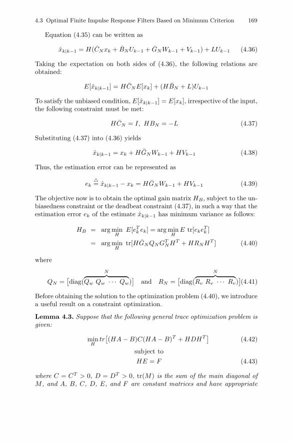
4.3 Optimal Finite Impulse Response Filters Based on Minimum Criterion 169

Equation (4.35) can be written as

xk|k−1 = H(CNxk + BNUk−1 + GNWk−1 + Vk−1) + LUk−1 (4.36)

Taking the expectation on both sides of (4.36), the following relations areobtained:

E[xk|k−1] = HCNE[xk] + (HBN + L)Uk−1

To satisfy the unbiased condition, E[xk|k−1] = E[xk], irrespective of the input,the following constraint must be met:

HCN = I, HBN = −L (4.37)

Substituting (4.37) into (4.36) yields

xk|k−1 = xk + HGNWk−1 + HVk−1 (4.38)

Thus, the estimation error can be represented as

ek= xk|k−1 − xk = HGNWk−1 + HVk−1 (4.39)

The objective now is to obtain the optimal gain matrix HB , subject to the un-biasedness constraint or the deadbeat constraint (4.37), in such a way that theestimation error ek of the estimate xk|k−1 has minimum variance as follows:

HB = arg minH

E[eTk ek] = arg min

HE tr[ekeT

k ]

= arg minH

tr[HGNQNGTNHT + HRNHT ] (4.40)

where

QN =[diag(

N︷ ︸︸ ︷Qw Qw · · · Qw)

]and RN =

[diag(

N︷ ︸︸ ︷Rv Rv · · · Rv)

](4.41)

Before obtaining the solution to the optimization problem (4.40), we introducea useful result on a constraint optimization.

Lemma 4.3. Suppose that the following general trace optimization problem isgiven:

minH

tr[(HA − B)C(HA − B)T + HDHT

](4.42)

subject toHE = F (4.43)

where C = CT > 0, D = DT > 0, tr(M) is the sum of the main diagonal ofM , and A, B, C, D, E, and F are constant matrices and have appropriate

170 4 Receding Horizon Filters

dimensions. The solution to the optimization problem (4.42) and (4.43) is asfollows:

H =[F B

] [ (ET Π−1E)−1ET Π−1

CAT Π−1(I − E(ET Π−1E)−1ET Π−1)

](4.44)

where Π= ACAT + D. H has an alternative representation as

H =[F B

] [W1,1 W1,2

WT1,2 W2,2

]−1 [ET

AT

]D−1 (4.45)

where

W1,1= ET D−1E (4.46)

W1,2= ET D−1A (4.47)

W2,2= AT D−1A + C−1 (4.48)

Proof. For convenience, partition the matrix H in (4.43) as

HT =[h1 h2 · · · hn

](4.49)

From HE = F , the sth unbiasedness constraint can be written as

ET hs = fs, 1 ≤ s ≤ n (4.50)

where fs is the sth column vector of F . In terms of the partitioned vector hs,the cost function (4.42) is represented as

n∑s=1

[(hT

s A − bTs )C(hT

s A − bTs )T + hT

s Dhs

](4.51)

where bs is the sth column vector of B. It can be seen that the sth constraint(4.50) and sth term in the summation (4.51) are dependent only on hs, nothp, p = s. Thus, the optimization problem (4.43) is reduced to n independentoptimization problems

minhs

(hTs A − bT

s )C(hTs A − bT

s )T + hTs Dhs (4.52)

subject toET hs = fs (4.53)

for 1 ≤ s ≤ n. Obtaining the solutions to each optimization problem (4.53)and putting them together, we can finally obtain the solution to (4.42) and(4.43).

In order to solve the optimization problem, we establish the following costfunction:

4.3 Optimal Finite Impulse Response Filters Based on Minimum Criterion 171

φs= (hT

s A − bTs )C(hT

s A − bTs )T + hT

s Dhs + λTs (ET hs − fs)

= hTs (ACAT + D)hs − bT

s CAT hs − hTs ACbs + bT

s Cbs

+ λTs (ET hs − fs) (4.54)

where λs is the sth vector of a Lagrange multiplier, which is associated withthe sth unbiased constraint. Under the constraint (4.53), hs will be chosen tooptimize (4.52) with respect to hs and λs for s = 1, 2, · · · , n.

In order to minimize φs, two necessary conditions

∂φs

∂hs= 0 and

∂φs

∂λs= 0

are necessary, which give

hs = (ACAT + D)−1(ACbs −12Eλs) = Π−1(ACbs −

12Eλs) (4.55)

where Π = ACAT + D and the inverse of Π is guaranteed since C > 0 andD > 0. Pre-multiplying (4.55) by ET , we have

ET hi = ET Π−1(ACbs −12Eλs) = fs (4.56)

where the second equality comes from (4.50). From (4.56), we can obtain

λs = 2(ET Π−1E)−1[ET Π−1ACbs − fs]

from which hs is represented as

hTs = [fT

s − bTs CAT Π−1E](ET Π−1E)−1ET Π−1 + bT

s CAT Π−1

by using (4.55). H is reconstructed from hs as follows:

H = BCAT Π−1[I − E(ET Π−1E)−1ET Π−1

]+ F (ET Π−1E)−1ET Π−1

=[F B

] [ (ET Π−1E)−1ET Π−1

CAT Π−1(I − E(ET Π−1E)−1ET Π−1)

](4.57)

Now, we shall derive a more compact form by using variables (4.46), (4.47),and (4.48). It is first noted that the nonsingularity of W1,1 is guaranteed toexist under the assumption that E is of a full rank. The first row block of thesecond block matrix in (4.57) can be represented using the defined variables(4.46)–(4.48) as

(ET Π−1E)−1ET Π−1

=(

ETND−1E − ET D−1A(AT D−1A + C−1)−1AT C−1E

)−1

×(

ET D−1 − ET D−1A(AT D−1A + C−1)−1AT D−1

)=(

W1,1 − W1,2W−12,2 WT

1,2

)−1

(ET D−1 − W1,2W−12,2 AT D−1) (4.58)

172 4 Receding Horizon Filters

It is observed from (4.46)–(4.48) that

CAT Π−1 = CAT (D−1ACAT + I)−1D−1

= (AT D−1A + C−1)−1AT D−1 = W2,2AT D−1

and

CAT Π−1E = W2,2AT D−1E = W−1

2,2 WT1,2

from which we obtain

CAT Π−1(I − E(ET Π−1E)−1ET Π−1)= W−1

2,2 AT D−1

− W−12,2 WT

1,2(W1,1 − W1,2W−12,2 WT

1,2)−1(ET D−1 − W1,2W

−12,2 AD−1)

= (W2,2 − WT1,2W

−11,1 W1,2)−1WT

1,2W−11,1 ED−1

+ (W2,2 − WT1,2W

−11,1 W1,2)−1AT D−1 (4.59)

where the second equality can be derived from

W−12,2 WT

1,2(W1,1 − W1,2W−12,2 WT

1,2)−1

= W−12,2 WT

1,2(I − W−11,1 W1,2W

−12,2 WT

1,2)−1W−1

1,1

= W−12,2 (I − W T

1,2W−11,1 W1,2W

−12,2 WT

1,2)−1WT

1,2

= (W2,2 − WT1,2W

−11,1 W1,2)−1WT

1,2W−11,1

and

W−12,2 − W−1

2,2 WT1,2(W1,1 − W1,2W

−12,2 WT

1,2)−1W1,2W

−12,2

= (W2,2 − WT1,2W

−11,1 W1,2)−1

Substituting (4.58) and (4.59) into (4.57) yields[(ET Π−1E)−1ET Π−1

CAT Π−1(I − E(ET Π−1E)−1ET Π−1)

]=[

(W1,1 − W1,2W−12,2 WT

1,2)−1 −Z

ZT (W2,2 − WT1,2W

−11,1 W1,2)−1

] [ET D−1

AT D−1

]=[

W1,1 W1,2

WT1,2 W2,2

]−1 [ET D−1

AT D−1

](4.60)

where Z= (W1,1 −W1,2W

−12,2 WT

1,2)−1W1,2W

−12,2 . Therefore, the gain matrix H

in (4.57) can be written as (4.45). This completes the proof.

By using the result of Lemma 4.3, the solution to the optimization problem(4.40) can be obtained according to the following correspondence:

4.3 Optimal Finite Impulse Response Filters Based on Minimum Criterion 173

A ←− GN

B ←− OC ←− QN

D ←− RN

E ←− CN

F ←− I

(4.61)

In the following theorem, the optimal filter gain HB is represented in anexplicit form.

Theorem 4.4. When A,C is observable and N ≥ n, the MVF filterxk|k−1 with a batch form on the horizon [k − N, k] is given as follows:

xk|k−1 = HB(Yk−1 − BNUk−1) (4.62)

with the optimal gain matrix HB determined by

HB = (CTNΞ−1

N CN )−1CTNΞ−1

N (4.63)

where Yk−1, Uk−1, CN , BN , and ΞN are given by (4.28), (4.29), (4.31),(4.32), and (4.34) respectively.

From Theorem 4.4, it can be known that the MVF filter xk|k−1 (4.62)processes the finite measurements and inputs on the horizon [k−N, k] linearlyand has the properties of unbiasedness and minimum variance by design. Notethat the optimal gain matrix HB (4.63) requires computation only on theinterval [0, N ] once and is time-invariant for all horizons. This means thatthe MVF filter is time-invariant. It is a general rule of thumb that, due to theFIR structure, the MVF filter may also be robust against temporary modellinguncertainties or round-off errors, as seen in Example 4.1.

It is true that even though the MVF filter xk|k−1 (4.62) is designed withnonzero Q and R, it has the deadbeat property, i.e. xk|k−1 = xk, when appliedto the following noise-free observable systems:

xi+1 = Axi + Bui (4.64)yi = Cxi (4.65)

If there is no noise on the horizon [k − N, k − 1], then xk|k−1 and xk becomedeterministic. Since xk|k−1 is unbiased, xk|k−1 must be equal to xk. Since MVFfilter (4.62) is obtained with nonzero Qw and Rv, it may be less sensitive tonoises or disturbances than existing deterministic deadbeat observers thatare obtained from (4.64) and (4.65), as seen in Example 4.2. The deadbeatproperty indicates finite convergence time, and thus fast tracking ability fornoise-free systems. Therefore, an MVF filter may have a faster tracking abilitythan an IIR filter even with noises.

An MVF filter can be used in many problems, such as fault detection anddiagnosis of various systems, manoeuvre detection and target tracking of fly-ing objects, and model-based signal processing.

174 4 Receding Horizon Filters

Recursive Form

In this section, the MVF filter xk|k−1 (4.62) with a batch form is representedin an iterative form for computational advantage in the case of nonsingularA.

First, the MVF filter xk|k−1 (4.62) will be represented in an iterative form.Define

Ωi= CT

i Ξ−1i Ci (4.66)

Then it can be represented in the following discrete Riccati Equation using[Lew86a]:

Ωi+1 = CTi+1Ξ

−1i+1Ci+1

= A−T

[Ci

C

]T (∆i +

[Ci

C

]A−1GQwGT A−T

[Ci

C

]T )−1[Ci

C

]A−1

= A−T

[Ci

C

]T (∆−1

i − ∆−1i

[Ci

C

]A−1G ×

I + GT A−T

[Ci

C

]T

∆−1i

×[

Ci

C

]A−1G

GT A−T

[Ci

C

]T

∆−1i

)−1[Ci

C

]A−1

=(

I − A−T

[Ci

C

]T

∆−1i

[Ci

C

]A−1G ×

I + GT A−T

[Ci

C

]T

∆−1i

×[

Ci

C

]A−1G

GT

)A−T

[Ci

C

]T

∆−1i

[Ci

C

]A−1

=(

I − A−T (Ωi + CT R−1v C)A−1G

I + GT A−T (Ωi + CT R−1

v C)

× A−1G

GT

)A−T

[Ci

C

]T

∆−1i

[Ci

C

]A−1

=(

I + A−T (Ωi + CT R−1v C)A−1GQwGT

)−1

× A−T

[Ci

C

]T

∆−1i

[Ci

C

]A−1 (4.67)

Finally, we have

Ωi+1 = [I + A−T (Ωi + CT R−1v C)A−1GQwGT ]−1

× A−T (Ωi + CT R−1v C)A−1 (4.68)

Since Ω1 in the batch form (4.66) can be expressed as

Ω1 = CT1 Ξ−1

1 C1 = (CA−1)T (CA−1GQwGT A−T CT + Rv)−1CA−1

= [I + A−T CT R−1v CA−1GQwGT ]−1A−T CT R−1

v CA−1

4.3 Optimal Finite Impulse Response Filters Based on Minimum Criterion 175

Ω0 = 0 should be satisfied to obtain the above Ω1 in Riccati Equation (4.68).Let

xk−N+i= CT

i Ξ−1i (Yk−N+i−1 − BiUk−N+i−1) (4.69)

where

Yk−N+i= [yT

k−N yTk−N+1 · · · yT

k−N+i]T

Uk−N+i= [uT

k−N uTk−N+1 · · · uT

k−N+i]T

Then, on the interval 0 ≤ i ≤ N − 1, the subsidiary estimate xk−N+i+1 attime k − N + i + 1 is obtained from the definition (4.69) as follows:

xk−N+i+1

= CTi+1Ξ

−1i+1(Yk−N+i − Bi+1Uk−N+i)

= CTi+1Ξ

−1i+1

([Yk−N+i−1 − BiUk−N+i−1

yk−N+i

]+[

Ci

C

]A−1Buk−N+i

)(4.70)

In (4.70), the matrix CTi+1Ξ

−1i+1 can be written as

CTi+1Ξ

−1i+1

= A−T

[Ci

C

]T (∆i +

[Ci

C

]A−1GQwGT A−T

[Ci

C

]T )−1

= A−T

[Ci

C

]T (∆−1

i − ∆−1i

[Ci

C

]A−1G

×

Q−1w + GT A−T

[Ci

C

]T

∆−1i

[Ci

C

]A−1G

−1

GT A−T

[Ci

C

]T

∆−1i

)=(

I − A−T

[Ci

C

]T

∆−1i

[Ci

C

]A−1G

×

Q−1w + GT A−T

[Ci

C

]T

∆−1i

[Ci

C

]A−1G

−1

GT

)A−T

[Ci

C

]T

∆−1i

=(

I − A−T (Ωi + CT R−1v C)A−1G

×

Q−1w + GT A−T (Ωi + CT R−1

v C)A−1G

−1

GT

)A−T

[Ci

C

]T

∆−1i

= [I + A−T (Ωi + CT R−1v C)A−1GQwGT ]−1A−T

[Ci

C

]T

∆−1i (4.71)

where ∆i is defined as

∆i=[

Ξi 00 Rv

]

176 4 Receding Horizon Filters

Substituting (4.71) into (4.70) gives

xk−N+i+1

= [I + A−T (Ωi + CT R−1v C)A−1GQwGT ]−1A−T

[Ci

C

]T

∆−1i

×([

Yk−N+i−1 − BiUk−N+i−1

yk−N+i

]+[

Ci

C

]A−1Buk−N+i

)= [I + A−T (Ωi + CT R−1

v C)A−1GQwGT ]−1A−T

× [CTi Ξ−1

i (Yk−N+i−1 − BiUk−N+i−1) + CT R−1v yk−N+i

+ (Ωi + CT R−1v C)A−1Buk−N+i]

and thus the subsidiary estimate xk−N+i becomes

xk−N+i+1 = [I + A−T (Ωi + CT R−1v C)A−1GQwGT ]−1A−T [xk−N+i

+ CT R−1v yk−N+i + (Ωi + CT R−1

v C)A−1Buk−N+i] (4.72)

xk−N+1 in a batch form (4.70) can be expressed as

xk−N+1 = CT1 Ξ−1

1 (yk−N − B1Uk−N )= (CA−1)T (CA−1GQwGT ACT + R)−1(yk−N + CA−1Buk−N )= [I + A−T CT R−1

v CA−1GQwGT ]−1A−T

× [CT R−1v yk−N+i + CT R−1

v CA−1Buk−N+i] (4.73)

where xk−N = 0 should be satisfied to obtain the same xk−N+1 in RiccatiEquation (4.72).

Therefore, from (4.69) and (4.72), the MVF filter xk|k−1 with an iterativeform is depicted in Figure 4.4 and given in the following theorem.

Theorem 4.5. Assume that A,C is observable and N ≥ n. Then theMVF filter xk|k−1 with an iterative form is given on the horizon [k −N, k] asfollows:

xk|k−1 = Ω−1N xk (4.74)

where ΩN and xk are obtained from (4.67) and (4.72) respectively.

The recursive filter (4.74) is depicted in Figure 4.4.

4.3 Optimal Finite Impulse Response Filters Based on Minimum Criterion 177

XX

Fig. 4.4. Obtaining the state from recursive equations

4.3.3 Minimum Variance Finite Impulse Response Filters withGeneral A

Batch Form

If it is assumed that the system matrix is nonsingular, then the derivationof the FIR filter becomes somewhat easy. Thus, many results are based onthese assumptions. These restrictions may prevent an FIR filter from beingapplied to many applications. For example, in the case of high-order systems,the system matrix may be a sparse matrix so that there is much chance tohave the singularity in the system matrix. Thus it is desirable to derive theFIR filter for general cases. In this section, the MVF filter is derived based onthe general systems that do not require the inverse of the system matrix.

The system (4.1) and (4.2) will be represented in a batch form on the mostrecent time interval [k − N, k], called the horizon. On the horizon [k − N, k],the finite number of measurements is expressed in terms of the state xk−N atthe initial time k − N on the horizon as follows:

Yk−1 = CNxk−N + BNUk−1 + GNWk−1 + Vk−1 (4.75)

where

Yk−1= [yT

k−N yTk−N+1 · · · yT

k−1]T (4.76)

Uk−1= [uT

k−N uTk−N+1 · · · uT

k−1]T (4.77)

Wk−1= [wT

k−N wTk−N+1 · · · wT

k−1]T

Vk−1= [vT

k−N vTk−N+1 · · · vT

k−1]T

and CN , BN , and GN are obtained from

178 4 Receding Horizon Filters

Ci=

⎡⎢⎢⎢⎢⎢⎣C

CACA2

...CAi−1

⎤⎥⎥⎥⎥⎥⎦ (4.78)

Bi=

⎡⎢⎢⎢⎢⎢⎣0 0 · · · 0 0

CB 0 · · · 0 0CAB CB · · · 0 0

......

......

...CAi−2B CAi−3B · · · CB 0

⎤⎥⎥⎥⎥⎥⎦ (4.79)

Gi=

⎡⎢⎢⎢⎢⎢⎣0 0 · · · 0 0

CG 0 · · · 0 0CAG CG · · · 0 0

......

......

...CAi−2G CAi−3G · · · CG 0

⎤⎥⎥⎥⎥⎥⎦ (4.80)

The noise term GNWk−1 +Vk−1 in (4.75) can be shown to be zero-mean withcovariance ΠN given by

ΠN = GNQN GTN + RN (4.81)

where QN and RN are given in (4.41). The current state xk can be representedusing the initial state xk−N on the horizon as

xk = ANxk−N +[AN−1G AN−2G · · · G

]Wk−1

+[AN−1B AN−2B · · · B

]Uk−1 (4.82)

Augmenting (4.75) and (4.82) yields the following linear model:[Yk−1

0

]=[

CN 0AN −I

] [xk−N

xk

]+[

BN

AN−1B · · · B

]Uk−1

+[

GN

AN−1G · · · G

]Wk−1 +

[Vk−1

0

](4.83)

Using Yk−1 (4.76) and Uk−1 (4.77), the FIR filter is represented as

xk|k−1 = HYk−1 + LUk−1 (4.84)

By using Equation (4.83), the FIR filter (4.35) can be rewritten as

4.3 Optimal Finite Impulse Response Filters Based on Minimum Criterion 179

xk|k−1 =[H −I

] [Yk−1

0

]+ LUk−1,

=[H −I

] [ CN 0AN −I

] [xk−N

xk

]+[H −I

] [ BN

AN−1B · · · B

]Uk−1

+[H −I

] [ GN

AN−1G · · · G

]Wk−1 +

[H −I

] [Vk−1

0

]+ LUk−1, (4.85)

and taking the expectation on both sides of (4.85) yields the following equa-tion:

E[xk|k−1] = (HCN − AN )E[xk−N ] + E[xk] +[H −I

]×[

BN

AN−1B · · · B

]Uk−1 + LUk−1

To satisfy the unbiased condition, i.e. E[xk|k−1] = E[xk], irrespective of theinitial state and the input, the following constraint is required:

HCN = AN (4.86)

L = −[H −I

] [ BN

AN−1B · · · B

](4.87)

Substituting (4.86) and (4.87) into (4.85) yields the somewhat simplified equa-tion as

xk|k−1 = xk + HGNWk−1 −[AN−1G · · · G

]Wk−1 + HVk−1

ek= xk|k−1 − xk = HGNWk−1 −

[AN−1G · · · G

]Wk−1 + HVk−1

Note that the error between the real state and the estimated state dependsonly on H, not L, so that we have only to find H optimizing the give perfor-mance criterion.

The objective now is to obtain the optimal gain matrix HB , subject to theunbiasedness constraints (4.86) and (4.87), in such a way that the estimationerror ek of the estimate xk|k−1 has minimum variance as follows:

HB = arg minH

E[eTk ek] = arg min

HE tr[ekeT

k ]

= arg minH

tr[ΦQNΦT + HRNHT ] (4.88)

where Φ = HGN −[AN−1G · · · G

].

By using the result of Lemma 4.3, the solution to the optimization problem(4.88) can be obtained according to the following correspondence:

180 4 Receding Horizon Filters

A ←− GN

B ←−[AN−1G · · · G

]C ←− QN

D ←− RN

E ←− CN

F ←− AN

W1,1 ←− CTNR−1

N CN

W1,2 ←− CTNR−1

N GN

W2,2 ←− GTNR−1

N GN + Q−1N

(4.89)

The filter gain L can be obtained from (4.87). In the following theorem, wesummarize what we have done so far.

Theorem 4.6. When A,C is observable and N ≥ n, for a general A, theMVF filter xk|k−1 with a batch form on the horizon [k − N, k] is given as

xk|k−1 =[AN AN−1G AN−2G · · · AG G

] [W1,1 W1,2

WT1,2 W2,2

]−1

×[

CTN

GTN

]R−1

N

(Yk−1 − BNUk−1

)+[AN−1B AN−2B AN−3B · · · AB B

]Uk−1 (4.90)

As can be seen in (4.90), the inverse of the system matrix A does not appearin the filter coefficients. The batch form proposed in this section requiresthe inversion computation of matrices ΞN and CT

NΞ−1N CN . The dimension

of these matrices becomes large as the horizon length N increases. To avoidthe inversion computation of large-dimensional matrices, the iterative form isproposed in the next section.

Recursive Form

Now we introduce how to obtain a recursive form without using the inverseof A. An system without inputs is concerned for simple derivation. Beforederiving the recursive form of the MVF filter for general systems, we shallintroduce a batch form of the Kalman filter.

Theorem 4.7. On the horizon [k−N k], the Kalman filter can be representedin a batch form as

xk|k−1 =[AN AN−1G AN−2G · · · AG G

] [W1,1 + P−1k−N W1,2

WT1,2 W2,2

]−1

×([

P−1k−N

0

]xk−N +

[CT

N

GTN

]R−1

N Yk

)(4.91)

4.3 Optimal Finite Impulse Response Filters Based on Minimum Criterion 181

where k−N is the initial time and the covariance and the estimated value forthe initial state on the horizon are given as Pk−N and xk−N respectively. Thesolution to Riccati equation for the Kalman filter is given as

Pk =[AN AN−1G AN−2G · · · AG G

] [W1,1 + P−1k−N W1,2

WT1,2 W2,2

]−1

×[AN AN−1G AN−2G · · · AG G

]T (4.92)

Proof. In time-invariant systems we can always assume, without a loss ofgenerality, that the initial time is 0. Therefore, for simple notations, 0 and Nwill be used instead of k−N and N . In other words, we will focus on obtainingxN |N−1 using the information on x0|−1, P0, and YN−1 where

Yi= [yT

0 yT1 · · · yT

i−1]T (4.93)

for 0 ≤ i ≤ N − 1.Define variables Li, Mi, and Ni as

Li=[Ai Ai−1G Ai−2G · · · AG G

](4.94)

Mi=[

CTi R−1

i Ci + P−10 CT

i R−1i Go

i

GoTi R−1

i Ci GoTi R−1

i Goi + Q−1

i

](4.95)

Ni=[

Mi−1 00 Q−1

w

](4.96)

Ti=[

P−10

0

]xk−i +

[CT

i

GTi

]R−1

i Yi (4.97)

where Ci and Gi are defined in (4.78)–(4.80) and Goi is the matrix which is

obtained by removing the last zero column block from Gi, i.e. Gi =[Go

i 0].

Using the defined variables (4.94)–(4.97), we can represent xN of (4.91)and PN of (4.92) as

xN = LNN−1N TN (4.98)

PN = LNN−1N LT

N (4.99)

First, we will try to derive the batch form of covariance matrix (4.92). Recallthat Riccati equation of the Kalman filter is

Pi+1 = APiAT + GQwGT − APiC

T (Rv + CPiCT )−1CPiA

T (4.100)

which is used to solve for the estimation error covariance matrix.Given an initial covariance matrix P0, we can calculate P1 from (4.100) as

follows:

P1 = AP0AT + GQwGT − AP0C

T (Rv + CP0CT )−1CP0A

T (4.101)= A(P−1

0 + CT R−1v C)−1AT + GQwGT (4.102)

=[A G

] [P−10 + CT R−1

v C 00 Q−1

w

]−1 [A G

]T (4.103)

182 4 Receding Horizon Filters

(4.103) can be written in terms of Li and Ni as

P1 = L1N−11 LT

1 (4.104)

By an induction method, Pi+1 will be calculated from Pi of the batch form,i.e. Pi = LiN

−1i LT

i . Before proceeding, we introduce the following relation:

Ni + LTi CT R−1

v CLi = Mi (4.105)

which is proved as follows. If Si is defined as

Si=[Ai−1G Ai−2G · · · AG G

](4.106)

then Li can be represented as

Li =[Ai Si

](4.107)

from which we have

LTi CT R−1

v CLi =[

AiT CT R−1v CAi AiT CT R−1

v CSi

STi CT R−1

v CAi STi CT R−1

v CSi

](4.108)

The four block elements in Mi can be expressed recursively:

CTi R−1

i Ci = CTi−1R

−1i−1Ci−1 + ATiCT R−1

v CAi (4.109)

CTi R−1

i Goi =

[CT

i−1R−1i−1G

oi−1 0

]+ ATiCT R−1

v CSi (4.110)

GoTi R−1

i Goi =

[GoT

i−1R−1i−1G

oi−1 0

0 0

]+ ST

i CT R−1v CSi (4.111)

Using (4.108) and (4.109)–(4.111), we have

Ni + LTi CT R−1

v CLi (4.112)

=

⎡⎣ CTi−1R

−1i−1Ci−1

[CT

i−1R−1i−1Gi−1 0

][CT

i−1R−1i−1Gi−1 0

]T [ GoTi−1R

−1i−1G

oi−1 + Q−1

i−1 00 Q−1

w

]⎤⎦+[

AiT CT R−1v CAi AiT CT R−1

v CSi

STi CT R−1

v CAi STi CT R−1

v CSi

](4.113)

=[

CTi R−1

i Ci CTi R−1

i Gi

GTi R−1

i Ci GTi R−1

i Gi + Q−1i

]= Mi (4.114)

Starting from (4.100) and using the relation (4.105), we obtain the Pi+1

of the batch form

Pi+1 = ALi

N−1

i − N−1i LT

i CT (Rv + CLiN−1i LT

i CT )−1CLiN−1i

LT

i A

+ GQwGT ,

= ALi(Ni + LTi CT R−1

v CLi)−1LTi A + GQwGT

= ALiM−1i LT

i A + GQwGT = Li+1N−1i+1L

Ti+1 (4.115)

4.3 Optimal Finite Impulse Response Filters Based on Minimum Criterion 183

Now, using the solution of Riccati equation, i.e. the covariance matrix repre-sented in the batch form, we obtain a batch form of the Kalman filter. Thedynamic equation for the Kalman filter is written as follows:

xi+1|i = Axi|i−1 + APiCT (Rv + CPiC

T )−1(yi − Cxi|i−1)

= (A − APiCT (Rv + CPiC

T )−1C)xi|i−1

+ APiCT (Rv + CPiC

T )−1yi (4.116)

where Pi is given by (4.92). To obtain a batch form of the Kalman filter, weshall also use an induction method.

First, by using (4.100), x1|0 will be obtained from x0|−1 and P0:

x1|0 = (A − AP0CT (Rv + CP0C

T )−1C)x0|−1 + AP0CT (Rv + CP0C

T )−1y0,

= A(I + P0CT R−1

v C)−1x0|−1 + AP0CT (Rv + CP0C

T )−1y0

= A(P−10 + CT R−1

v C)−1P−10 x0|−1 + AP0C

T (I + R−1v CP0C

T )−1R−1v y0,

= A(P−10 + CT R−1

v C)−1(x0|−1 + CT R−1v y0)

In terms of Li, Ni, and Ti, x1|0 can be written as

x1|0 = L1N−11 T1 (4.117)

By an induction method, xi+1|i will be calculated from xi|i−1 of the batchform, i.e. xi|i−1 = LiN

−1i Ti.

First, observe that the first and second terms on the right-hand side of theKalman filter reduce to

A − APiCT (Rv + CPiC

T )−1C

xi|i−1

= ALi

N−1

i − N−1i LT

i CT (Rv + CLiN−1i LT

i CT )−1CLiN−1i

Ti

= ALi

Ni + LT

i CT R−1v CLi

−1

Ti = ALiM−1i Ti (4.118)

and

APiCT (Rv + CPiC

T )−1yi

= ALiN−1i LT

i CT (Rv + CLiN−1i LT

i CT )−1yi

= ALi(I + N−1i LT

i CT R−1v CLi)−1N−1

i LTi CT R−1

v yi

= ALi(Ni + LTi CT R−1

v CLi)−1LTi CT R−1

v yi

= ALiM−1i LT

i CT R−1v yi (4.119)

respectively. Substituting (4.118) and (4.119) into the Kalman filter yields

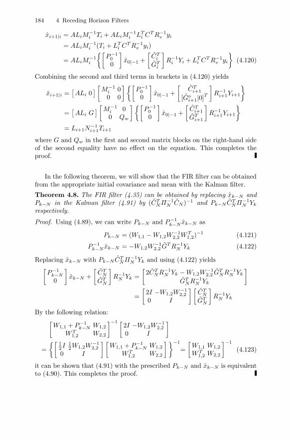
184 4 Receding Horizon Filters

xi+1|i = ALiM−1i Ti + ALiM

−1i LT

i CT R−1v yi

= ALiM−1i (Ti + LT

i CT R−1v yi)

= ALiM−1i

[P−1

0

0

]x0|−1 +

[CT

i

GTi

]R−1

i Yi + LTi CT R−1

v yi

(4.120)

Combining the second and third terms in brackets in (4.120) yields

xi+1|i =[ALi 0

] [M−1i 00 0

][P−1

0

0

]x0|−1 +

[CT

i+1

[Goi+1|0]T

]R−1

i+1Yi+1

=[ALi G

] [M−1i 00 Qw

][P−1

0

0

]x0|−1 +

[CT

i+1

GTi+1

]R−1

i+1Yi+1

= Li+1N

−1i+1Ti+1

where G and Qw in the first and second matrix blocks on the right-hand sideof the second equality have no effect on the equation. This completes theproof.

In the following theorem, we will show that the FIR filter can be obtainedfrom the appropriate initial covariance and mean with the Kalman filter.

Theorem 4.8. The FIR filter (4.35) can be obtained by replacing xk−N andPk−N in the Kalman filter (4.91) by (CT

NΠ−1N CN )−1 and Pk−N CT

NΠ−1N Yk

respectively.

Proof. Using (4.89), we can write Pk−N and P−1k−N xk−N as

Pk−N = (W1,1 − W1,2W−12,2 WT

1,2)−1 (4.121)

P−1k−N xk−N = −W1,2W

−12,2 GT R−1

N Yk (4.122)

Replacing xk−N with Pk−N CTNΠ−1

N Yk and using (4.122) yields[P−1

k−N

0

]xk−N +

[CT

N

GTN

]R−1

N Yk =[

2CTNR−1

N Yk − W1,2W−12,2 GT

NR−1N Yk

GTNR−1

N Yk

]=[

2I −W1,2W−12,2

0 I

] [CT

N

GTN

]R−1

N Yk

By the following relation:[W1,1 + P−1

k−N W1,2

WT1,2 W2,2

]−1 [2I −W1,2W

−12,2

0 I

]=[

12I 1

2W1,2W−12,2

0 I

] [W1,1 + P−1

k−N W1,2

WT1,2 W2,2

]−1

=[

W1,1 W1,2

WT1,2 W2,2

]−1

(4.123)

it can be shown that (4.91) with the prescribed Pk−N and xk−N is equivalentto (4.90). This completes the proof.

4.3 Optimal Finite Impulse Response Filters Based on Minimum Criterion 185

In the following lemma, xk−N and Pk−N in Theorem 4.8 are shown to becomputed recursively.

Lemma 4.9. xk−N and Pk−N in Theorem 4.8 can be computed from

xk−N = (CT R−1v C + PN )−1(CT R−1

v yk−N + ωN ) (4.124)Pk−N = (CT R−1

v C + PN )−1 (4.125)

where PN and wN can be obtained from the following recursive equations:

Pi+1 = AT CT R−1v CA + AT PiA

− AT (CT R−1v C + Pi)G

Q−1

w + GT AT (CT R−1v C + Pi)AG

−1

× GT (CT R−1v C + Pi)A (4.126)

and

ωi+1 = AT CT Rvyk−i + Aωi

− AT (CT R−1v C + Pi)G

Q−1

w + GT AT (CT R−1v C + Pi)AG

−1

× GT (CT R−1v yk−i + ωi) (4.127)

with P1 = 0, w1 = 0, and 1 ≤ i ≤ N − 1.

Proof. Define Ci, Ni, Πi, Pi, and ωi as

Ci=

⎡⎢⎢⎢⎢⎢⎣CA...

CAi−3

CAi−2

CAi−1

⎤⎥⎥⎥⎥⎥⎦ =[

C

Ci−1

]A (4.128)

Ni=

⎡⎢⎢⎢⎣CG 0 · · · 0

CAG CG · · · 0...

......

...CAi−2G CAi−3G · · · CG

⎤⎥⎥⎥⎦ (4.129)

Πi= NiQi−1N

Ti + Ri−1 (4.130)

Pi= CT

i Π−1i Ci (4.131)

wi= CT

i Π−1i Yk−i+1,k−1 (4.132)

Yk−i+1,k−1= [yT

k−i+1 yTk−i+2 · · · yT

k−1]T (4.133)

Using (4.128)–(4.131), Pk−N and xk−N can be represented as

186 4 Receding Horizon Filters

Pk−N = (CTNΠ−1

N CN )−1 = (CT R−1v C + PN )−1 (4.134)

xk−N = Pk−N (CT R−1v yk−N + CT

N Π−1N Yk−N+1,k−1) (4.135)

In order to obtain xk−N and Pk−N , we have only to know CTN Π−1

N Yk−N+1,k−1

and PN , which are calculated recursively.First, a useful equality is introduced for obtaining the recursive form:

Π−1i+1 = (Ni+1QiN

Ti+1 + Ri)−1

=([

Rv 00 Πi

]+[

C

Ci

]GQwGT

[C

Ci

]T )−1

= ∆−1i − ∆−1

i

[C

Ci

]G

Q−1

w + GT AT

[C

Ci

]T

∆−1i

[C

Ci

]AG

−1

GT

[C

Ci

]∆−1

i (4.136)

where

∆i =[

Rv 00 Πi

](4.137)

Pre- and post-multiplying on both sides of (4.136) by[C

Ci

]A (4.138)

we have

Pi+1 = AT CT R−1v CA + AT PiA

− AT (CT R−1v C + Pi)G

Q−1

w + GT AT (CT R−1v C + Pi)AG

−1

× GT (CT R−1v C + Pi)A (4.139)

Pre-multiplying on both sides of (4.136) by (4.138), we obtain another recur-sive equation:

ωi+1 = AT CT Rvyk−i + Aωi

− AT (CT R−1v C + Pi)G

Q−1

w + GT AT (CT R−1v C + Pi)AG

−1

× GT (CT R−1v yk−i + ωi) (4.140)

After obtaining PN from (4.139), we can calculate Pk−N from (4.134). xk−N

in (4.135) can be obtained from Pk−N and ωN that comes from (4.140). Thiscompletes the proof.

4.3 Optimal Finite Impulse Response Filters Based on Minimum Criterion 187

In the following theorem, we summarize what we have done so far.

Theorem 4.10. For general A, the MVF filter is given on the horizon [k −N, k] as follows:

xk|k−1 = βk (4.141)

where βi is obtained from the following recursive equations:

βk−N+i+1 = Aβk−N+i + APiCT (Rv + CPiC

T )−1(yk−N+i − Cβk−N+i)= (A − APiC

T (Rv + CPiCT )−1C)βk−N+i

+ APiCT (Rv + CPiC

T )−1yk−N+i (4.142)Pi+1 = APiA

T + GQwGT − APiCT (Rv + CPiC

T )−1CPiAT (4.143)

Here, P0 = (CT R−1v C + PN )−1 and βk−N = P0(CT R−1

v yk−N + ωN ). PN andωN are obtained from (4.139) and (4.140) respectively.

Note that (4.142) and (4.143) are in a form of the Kalman filter with aspecial initial condition. The recursive filter in Theorem 4.10 is depicted inFigure 4.5.

XX

Fig. 4.5. Backward and forward estimations for general matrix A

188 4 Receding Horizon Filters

4.3.4 Numerical Examples for Minimum Variance Finite ImpulseResponse Filters

Example 4.1: Robustness of Minimum Variance Finite Impulse Re-sponse Filters

To demonstrate the validity of the MVF filter, numerical examples on thediscretized model of an F-404 engine [EWMR94] are presented via simulationstudies. The corresponding dynamic model is written as

xk+1 =

⎡⎣0.9305 + δk 0 0.11070.0077 0.9802 + δk −0.01730.0142 0 0.8953 + 0.1δk

⎤⎦xk +

⎡⎣111

⎤⎦wk

yk =[

1 + 0.1δk 0 00 1 + 0.1δk 0

]xk + vk (4.144)

where δk is an uncertain model parameter. The system noise covariance Qw is0.02 and the measurement noise covariance Rv is 0.02. The horizon length istaken as N = 10. We perform simulation studies for the system (4.144) witha temporary modelling uncertainty.

As mentioned previously, the MVF filter is believed to be robust againsttemporary modelling uncertainties since it utilizes only finite measurementson the most recent horizon. To illustrate this fact and the fast convergence,the MVF filter and the Kalman filter are designed with δk = 0 and comparedwhen a system actually has a temporary modelling uncertainty. The uncertainmodel parameter δk is considered as

δk =

0.1, 50 ≤ k ≤ 1000, otherwise (4.145)

Figure 4.6 compares the robustness of two filters given temporary mod-elling uncertainty (4.145) for the second state related to turbine temperature.This figure shows that the estimation error of the MVF filter is remarkablysmaller than that of the Kalman filter on the interval where modelling un-certainty exists. In addition, it is shown that the convergence of estimationerror is much faster than that of the Kalman filter after temporary modellinguncertainty disappears. Therefore, it can be seen that the suggested MVFfilter is more robust than the Kalman filter when applied to systems with amodel parameter uncertainty.

Example 4.2: Comparison with Deadbeat Infinite Impulse ResponseFilters

It is known that the MVF filter has the deadbeat property without exter-nal disturbances. Via numerical simulation, we compare the MVF filter with

4.3 Optimal Finite Impulse Response Filters Based on Minimum Criterion 189

0 50 100 150 200 250−0.5

0

0.5

1

1.5

2

2.5

3

Time

Est

imat

ion

erro

r

Kalman filter

MVF filter

Fig. 4.6. Estimation errors of MVF filter and Kalman filter

the conventional deadbeat IIR filter, which is known to be sensitive to externaldisturbance.

From the following simple model:

xi+1 = Axi (4.146)yi = Cxi (4.147)

the deadbeat filter of the partial state zi = Nxi will be obtained as

wi+1 = Aowi + Lyi (4.148)zi = Mwi (4.149)

where zi estimates zi exactly in a finite time irrespective of the initial stateerror. First, it is assumed that there exist matrices W and Ao such that

WA = AoW + LC , N = MW, Ado = 0 (4.150)

for some positive integer d. Letting ei = wi − Wxi, we have

ei+1 = wi+1 − Wxi+1 = Aowi + Lyi − WAxi

= Aowi + LCxi − WAxi = Aowi − AoWxi = Aoei (4.151)

and the estimation error zi−zi is represented as Nxi−Mwi = MWxi−Mwi =−Mei. According to (4.150) and (4.151), ei should be zero in a finite time

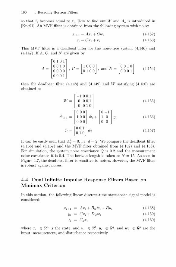
190 4 Receding Horizon Filters

so that zi becomes equal to zi. How to find out W and Ao is introduced in[Kuc91]. An MVF filter is obtained from the following system with noise:

xi+1 = Axi + Gwi (4.152)yi = Cxi + vi (4.153)

This MVF filter is a deadbeat filter for the noise-free system (4.146) and(4.147). If A, C, and N are given by

A =

⎡⎢⎢⎣0 1 0 10 0 1 00 0 0 00 0 0 1

⎤⎥⎥⎦ , C =[

1 0 0 00 1 0 0

], and N =

[0 0 1 00 0 0 1

](4.154)

then the deadbeat filter (4.148) and (4.149) and W satisfying (4.150) areobtained as

W =

⎡⎣−1 0 0 10 0 0 10 0 1 0

⎤⎦ (4.155)

wi+1 =

⎡⎣0 0 01 0 00 0 0

⎤⎦ wi +

⎡⎣0 −11 00 0

⎤⎦ yi (4.156)

zi =[

0 0 10 1 0

]wi (4.157)

It can be easily seen that A2o = 0, i.e. d = 2. We compare the deadbeat filter

(4.156) and (4.157) and the MVF filter obtained from (4.152) and (4.153).For simulation, the system noise covariance Q is 0.2 and the measurementnoise covariance R is 0.4. The horizon length is taken as N = 15. As seen inFigure 4.7, the deadbeat filter is sensitive to noises. However, the MVF filteris robust against noises.

4.4 Dual Infinite Impulse Response Filters Based onMinimax Criterion

In this section, the following linear discrete-time state-space signal model isconsidered:

xi+1 = Axi + Bwwi + Bui (4.158)yi = Cxi + Dwwi (4.159)zi = Czxi (4.160)

where xi ∈ n is the state, and ui ∈ l, yi ∈ q, and wi ∈ p are theinput, measurement, and disturbance respectively.

4.4 Dual Infinite Impulse Response Filters Based on Minimax Criterion 191

15 20 25 30 35 40 45 50 55−1

0

1

2

3

4

5

6

7

Deadbeat filter

MVF filter

Fig. 4.7. Comparison between deadbeat filter and MVF filter

Before we introduce a filter for (4.158) and (4.159), we will compare theH∞ control with the H∞ filter and investigate the structural differences be-tween them.

The H∞ control (2.146) with a zero reference signal and terminal time if ,is given by

u∗i = −R−1BT Λ−1

i+1,ifMi+1,if

Axi (4.161)

where Riccati equation is given by

Mi,if= AT [I + Mi+1,if

(BR−1BT − γ−2BwR−1w BT

w)]−1Mi+1,ifA + Q

= AT Mi+1,ifA − AT Mi+1,if

[(BR−1BT − γ−2BwR−1w BT

w)Mi+1,if

+ I]−1(BR−1BT − γ−2BwR−1w BT

w)Mi+1,ifA + Q (4.162)

Use the following relation:

BR−1BT − γ−2BwR−1w BT

w =[B Bw

] [R 00 Rw − γ2

]−1 [BT

BTw

]we have

192 4 Receding Horizon Filters

Mi,if= AT Mi+1,if

A − AT Mi+1,if

[B Bw

]×[

BT

BTw

]Mi+1,if

[B Bw

]+[

R 00 Rw − γ2

]−1−1[BT

BTw

]Mi+1,if

A

+ Q (4.163)

with

Mif ,if= Qf (4.164)

Meanwhile, the receding horizon H∞ control is given by

u∗i = −R−1BT Λ−1

1,NM1,NAxi (4.165)

where M1,N is computed from (4.163) with the terminal condition (4.164) byreplacing if with N . The gain matrices in (4.161) are time-varying, but thegain M1 in the receding horizon control (4.165) is fixed. That is, M1 is frozenat the time 1.

The standard H∞ filter can be written from (2.201) as

xi+1|i = Axi|i−1 + Bui + Li(yi − Cxi|i−1) (4.166)zi = Czxi|i−1 (4.167)

where

Li = ASiΓ−1i CT (4.168)

and the matrices Si and Γi are given by

Si+1 = ASiΓ−1i AT + BwBT

w (4.169)Γi = I + (CT C − γ−2CT

z Cz)Si (4.170)

where S0 = 0. The recursive equation (4.169) with respect to Si can be writtenas

Si+1 = ASiAT − ASi

[CT CT

z

](4.171)

×[

CCz

]Si

[CT CT

z

]+[

I 00 −γ2I

]−1−1[CCz

]SiA

T + BwBTw (4.172)

The H∞ filter is said to be dual to the H∞ control in the sense that two Ric-catti equations become the same as each other if some variables are changed,such as

A ←→ AT

B ←→ CT

Bw ←→ CTz

Q ←→ BwBTw

R ←→ IMi ←→ Si

(4.173)

4.4 Dual Infinite Impulse Response Filters Based on Minimax Criterion 193

Note that indexes of Mi+1 and Qi are based on backward and forward compu-tations respectively. We can see that the filter gain in (4.168) and the controlgain in (4.161) are similar to each other in the sense that the transpose of thecontrol gain replaced by (4.173) is the same as the filter gain in (4.168). Inthat view, the corresponding closed-loop system matrices of the H∞ controland the H∞ filter are also similar. It is noted that the properties of the H∞filter can be obtained from that of the dual to the H∞ control, since they arestructurally dual.

Likewise, we can introduce the dual filter to the receding horizon H∞control as follows:

xi+1|i = Axi|i−1 +[ASN [I + (CT C − γ−2CT

z Cz)SN ]−1CT

]× (yi − Cxi|i−1) (4.174)

where SN is obtained from (4.169). It turns out that the new filter (4.174) isjust the H∞ filter with a frozen gain from (4.166). This filter will be called thedual filter to the RH H∞ control or the H∞ filter with frozen gains throughoutthis book.

By using the duality (4.173), the inequality (3.234) in Theorem 3.15 ischanged to

K ≥ BwBTw + LLT

− ΓfΓTf + (A − LC + ΓfCz)K(A − LC + ΓfCz)T (4.175)

where matrices L and K correspond to H and Qf in (3.234) and Γf =γ−2AK(I + (CT C − γ−2CT

z Cz)K)−1CTz .

The stability of the dual filter to the RH H∞ control can be obtained.

Theorem 4.11. The dual filter to the RH H∞ control is stabilized if thereexist K and L satisfying (4.175). In other words, the following matrix is Hur-witz:

A − ASN [I + CT C − γ−2CTz CzSN ]−1CT C

where SN is the solution calculated from (4.169) with S0 = K.

Proof. The closed-loop system matrix of the filter is as follows:

A − ASN [I + (CT C − γ−2CTz Cz)SN ]−1CT C

= A[I − SN [I + (CT C − γ−2CTz Cz)SN ]−1CT C] (4.176)

where the transpose of the right side is

[I − CT CI + SN (CT C − γ−2CTz Cz)−1SN ]AT (4.177)

The matrix (4.176) is stable if and only if its transpose (4.177) is stable.

194 4 Receding Horizon Filters

Compare (4.177) with the closed-loop system matrix of the control

[I − BBT I + MN (BBT − γ−2BwBTw)−1MN ]A (4.178)

which is obtained with the changes listed in (4.173) and in this case Si =MN+1−i and K0 = MN . Therefore, the above result follows from Theorem3.15. This completes the proof.

The error covariance of the dual filter to the receding horizon H∞ control isbounded above by a constant matrix as in the following theorem.

Theorem 4.12. If there exist K and L satisfying (4.175), then the dual IIRfilter xi has the following bound:∑∞

i=i0eT

i ei∑∞i=i0

wTi wi

≤ γ2 (4.179)

Proof. The error dynamics can be represented as

ei+1 = (A − LNC)ei + (Bw − LNDw)wi (4.180)

where LN is defined in (4.168). Let the function Vi be defined by

Vi = eTi Kei (4.181)

where K is positive definite. ei0 is assumed to be zero. Then we have

J =∞∑

i=i0

[eT

i ei − γ2wTi wi

]≤

∞∑i=i0

[eT

i ei − γ2wTi wi

]+V∞ − Vi0

≤∞∑

i=i0

[eT

i ei − γ2wTi wi + eT

i+1Kei+1 − eTi Kei

]

=[

ei

wi

]T

Θ

[ei

wi

]≤ 0 (4.182)

where

Θ =

[(A − LNC)T K(A − LNC) − K + I (A − LNC)T K(Bw − LNDw)

(Bw − LNDw)T K(A − LNC) (Bw − LNDw)T K(Bw − LNDw) − γ2I

]and the negative semidefiniteness of Θ is proved in a similar way to the costmonotonicity of the RH H∞ control in Theorem 3.22. This completes theproof.

4.5 Finite Impulse Response Filters Based on Minimax Criterion 195

4.5 Finite Impulse Response Filters Based on MinimaxCriterion

4.5.1 Linear Unbiased Finite Impulse Response Filters

In this section, the FIR filter without a priori initial state information repre-sented by

xk|k−1 =k−1∑

i=k−N

Hk−iyi +k−1∑

i=k−N

Lk−iui (4.183)

is introduced for deterministic systems (4.158) and (4.159).The system (4.158) and (4.159) will be represented in a standard batch

form on the most recent time interval [k − N, k], called the horizon. On thehorizon [k−N, k], the finite number of measurements is expressed in terms ofthe state xk at the current time k as follows:

Yk−1 = CNxk + BNUk−1 + GNWk−1 + DNWk−1 (4.184)

where Yk−1, Uk−1, Wk−1, CN , BN , and GN are given by (4.28), (4.29), (4.30),(4.31), (4.32), and (4.33) respectively and DN is defined by

Di=[diag(

i︷ ︸︸ ︷D D · · · D)

]=[diag(Di−1,D)

](4.185)

1 ≤ i ≤ N (4.186)

An FIR filter with a batch form for the current state xk can be expressedas a linear function of the finite measurements Yk−1 (4.28) and inputs Uk−1

(4.29) on the horizon [k − N, k] as follows:

xk|k−1= HYk−1 + LUk−1 (4.187)

where H and L are gain matrices of a linear filter. It is noted that the filterdefined in (4.187) is an FIR structure without the requirement of any a prioriinformation about the horizon initial state xk−N .

Substituting (4.184) into (4.187) yields

xk|k−1 = HYk−1 + LUk−1

= H(CNxk + BNUk−1 + GNWk−1 + DNWk−1) + LUk−1 (4.188)

Among multiple H and L, we want to choose one that satisfies the followingrelation:

xk|k−1 = xk for any xk−N and any Uk−1 (4.189)

for a zero disturbance wi = 0. For stochastic systems, the unbiasedness con-straint E[xk|k−1] = E[xk] is an accepted requirement for the filter. If noises

196 4 Receding Horizon Filters

become zero on the horizon [k−N, k−1], then xk|k−1 and xk become determin-istic values, i.e. xk|k−1 = xk. For the corresponding property, if disturbancesbecome zero on the horizon [k − N, k − 1], then we have

xk+1 = Axk + Buk (4.190)yk = Cxk (4.191)

where we require xk|k−1 = xk. This is called a deadbeat condition and themodel (4.190) and (4.191) is called a nominal model. It is noted that, con-ventionally, noises are assumed to have zero mean and thus noises fluctuatearound zero. Likewise, the disturbance is assumed to fluctuate around zero.The relation (4.189) is called an unbiased condition in the deterministic sense,as seen in Figure 4.8.

Fig. 4.8. Deadbeat property without disturbance

In the case of wi = 0 we have

xk|k−1 = H(CNxk − BNUk−1) + LUk−1 (4.192)

Therefore, the following constraints are required for the unbiased condition:

HCN = I and L = −HBN (4.193)

which will be called the unbiased constraint. The FIR filter with the unbiasedconstraints for the current state xk can be expressed as

xk|k−1 = H(Yk−1 − BNUk−1) (4.194)

and substituting (4.193) into (4.188) yields

ek= xk − xk|k−1 = H(GN + DN )Wk−1 (4.195)

4.5 Finite Impulse Response Filters Based on Minimax Criterion 197

4.5.2 L2-E Finite Impulse Response Filters

The objective now is to obtain the optimal gain matrices H and L in sucha way that the worst-case gain between the estimation error of the estimatexk|k−1 and disturbance has a minimum value as follows:

minH,L

maxwi

[xk − xk|k−1]T [xk − xk|k−1]∑Ni=1 wT

k−iwk−i

(4.196)

The numerator of the performance criterion (4.196) considers only the currentestimation error. The FIR filter obtain from Equation (4.196) will be calledan L2 − E FIR (LEF) filter. The H and L coming from the performancecriterion (4.196) are dependent on system parameters such as A, B, C, andG, not dependent on any specific real disturbances.

By using (4.195), (4.196) can be written as

minH,L

maxWk−1

WTk−1(GN + DN )T HT H(GN + DN )Wk−1

WTk−1Wk−1

= minH,L

λmax

[(GN + DN )T HT H(GN + DN )

]= min

H,Lλmax

[H(GN + DN )(GN + DN )T HT

](4.197)

for H and L satisfying (4.193).Before obtaining the solution to the optimization problem (4.197), we in-

troduce a useful result in the following lemma.

Lemma 4.13. Suppose that the following general maximum eigenvalue opti-mization problem is given:

minH

λmax

[(HA − B)C(HA − B)T

](4.198)

subject toHE = F (4.199)

where C = CT > 0, D = DT > 0, and A, B, C, D, E, and F are constantmatrices and have appropriate dimensions. The solution to the optimizationproblem (4.198) and (4.199) is given by

H =[BCAT + (F − BCAT Π−1E)(ET Π−1E)−1ET

]Π−1 (4.200)

where Π = ACAT .

Proof. If there exists an HB such that

(HBA − B)C(HBA − B)T ≤ (HA − B)C(HA − B)T (4.201)

198 4 Receding Horizon Filters

where HE = HBE = F and H is arbitrary, we have

αT [(HBA − B)C(HBA − B)T ]α = λmax[(HBA − B)C(HBA − B)T ]αT α

≤ αT (HA − B)C(HA − B)T α

= λmax[(HA − B)C(HA − B)T ]αT α (4.202)

for the vector α that is an eigenvector of (HBA − B)C(HBA − B)T corre-sponding to λmax(HBA−B)C(HBA−B)T . Since α is nonzero, the followinginequality is obtained from (4.202):

λmax[(HBA − B)C(HBA − B)T ] ≤ λmax[(HA − B)C(HA − B)T ] (4.203)

which means that HB is the solution to the optimization problem (4.198) and(4.199).

Thus, we try to find out HB such that the inequality (4.201) is satisfied.In order to make the problem tractable, we change the inequality (4.201) toa scalar one as

vT (HBA − B)C(HBA − B)T v ≤ vT (HA − B)C(HA − B)T v (4.204)

for arbitrary vector v. It can be seen from the inequality (4.204) that theminimum value of vT

[(HA−B)C(HA−B)T

]v is the left side of the inequality

(4.204).Now, all that we have to do is to find the minimum value of right side of

the inequality (4.204) with respect to H and show that it is the same as theleft side of (4.204). The right side of (4.204) can be written as

(wT A − vT B)C(wT A − vT B)T (4.205)

where HT v = w. From HE = F in (4.199), w should satisfy

ET w = FT v (4.206)

Now, the following cost function to be optimized is introduced:

φ = (wT A − vT B)C(wT A − vT B)T + λT (ET w − FT v) (4.207)

where λ is the vector of a Lagrange multiplier. In order to minimize φ, twonecessary conditions

∂φ

∂w= 0,

∂φ

∂λ= 0 (4.208)

are required, which give

w = (ACAT )−1(ACBT v + Eλ) (4.209)

Substituting (4.209) into (4.206) yields

4.5 Finite Impulse Response Filters Based on Minimax Criterion 199

λ = (ET Π−1E)−1[−ET Π−1ACBT v + FT v] (4.210)

where Π = ACAT . Thus, w is obtained as

w = Π−1ACBT + E(ET Π−1E)−1(−ET Π−1ACBT + FT )v (4.211)

Since HT v = w, H can be written as (4.200). This completes the proof.

By using the result of Lemma 4.3, the solution to the optimization problem(4.197) can be obtained according to the following correspondences:

A ←− GN + DN

B ←− OC ←− IE ←− CN

F ←− IΠ ←− (GN + DN )(GN + DN )T

(4.212)

The filter gain L can be obtained from (4.193). In the following theorem, wesummarize what we have done so far.

The following theorem provides the solution to the optimal criterion(4.196) with the unbiased condition (4.193).

Theorem 4.14. Assume that A,C of the given system is observable. TheLEF filter is as follows:

xk|k−1 = (CTNΞ−1

N CN )−1CTNΞ−1

N (Yk−1 − BNUk−1) (4.213)

where

Ξi= GiG

Ti + DiD

Ti

=[

Gi−1GTi−1 + Di−1D

Ti−1 0

0 I

]+[

Ci−1

C

]A−1GGT A−T

[Ci−1

C

]T

=[

Ξi−1 00 I

]+[

Ci−1

C

]A−1GGT A−T

[Ci−1

C

]T

(4.214)

Note that the optimum gain matrix HB (4.196) requires computation onlyon the interval [0, N ] once and is time-invariant for all horizons. It is notedthat the estimation (4.213) holds for k ≥ k0 + N .

The LEF filter xk|k−1 has the unbiased property when applied to thenominal systems without disturbances (4.190) and (4.191), whereas the LEFfilter xk|k−1 is obtained from systems (4.158) and (4.159) with an additivesystem and measurement disturbances wk. The deadbeat property of the LEFfilter is given in the following corollary.

200 4 Receding Horizon Filters

Corollary 4.15. Assume that A,C is observable and N ≥ n. Then, theLEF filter xk|k−1 given by (4.213) provides the exact state when there are nodisturbances on the horizon [k − N, k].

Proof. When there are no disturbances on the horizon [k − N, k], Yk−1 −BNUk−1 is determined by the current state xk as Yk−1 − BNUk−1 = CNxk.Therefore, the following is true:

xk|k−1 = HB(Yk−1 − BNUk−1)

= (CTNΞ−1

N CN )−1CTNΞ−1

N CNxk

= xk

This completes the proof.

Note that the above deadbeat property indicates finite convergence timeand fast tracking ability of the LEF filter. Thus, it can be expected that theapproach would be appropriate for fast estimation and detection of signalswith unknown times of occurrence, which arise in many problems, such asfault detection and diagnosis of various systems, manoeuvre detection, targettracking of flying objects, etc.

In this section, the LEF filter xk|k−1 in batch form is represented in aniterative form, for computational advantage, and then shown to be similarin form to the MVF filter with unknown horizon initial state presented in[HKK01][KKH02].

Theorem 4.16. Assume that A,C is observable and N ≥ n. Then, theLEF filter xk|k−1 is given on the horizon [k − N, k] as follows:

xk|k−1 = Ω−1N xk (4.215)

where k ≥ k0 + N and ΩN and xk are obtained from following recursiveequations:

Ωi+1 = [I + A−T (Ωi + CT C)A−1GGT ]−1A−T (Ωi + CT C)A−1 (4.216)

xk−N+i+1 = [I + A−T (Ωi + CT C)A−1GGT ]−1A−T

[xk−N+i + CT yk−N+i + (Ωi + CT C)A−1Buk−N+i] (4.217)

with xk−N = 0 and Ω0 = 0.

Proof. If Qw and Rv are replaced with unit matrices in the MVF filter, thenthe proof is the same as that of Theorem 4.5.

4.5 Finite Impulse Response Filters Based on Minimax Criterion 201

It is surprising to observe that the LEF filter xk|k−1 (4.215) with an iterativeform is the same as the MVF filter with unknown horizon initial state in[KKP99], where the covariances of the system noise and the measurementnoise are taken as unit matrices.

To summarize, the LEF filter is linear with the most recent finite measure-ments and inputs, does not require a priori information about the horizoninitial state, and has the unbiased property. Thus, it is surprising, in that aclosed-form solution exists even with the unbiased condition. The LEF filtercan be represented in both a standard batch form and an iterative form thathas computational advantages. The LEF filter with the FIR structure for de-terministic systems is similar in form to the existing RHUFF for stochasticsystems with the unit covariance matrices of both the system noise and themeasurement noise. Furthermore, owing to the FIR structure, the LEF filter isbelieved to be robust against temporary modelling uncertainties or numericalerrors, whereas other minimax filters and H∞ filters with an IIR structuremay show poor robustness in these cases.

The LEF filter will be very useful for many signal processing problemswhere signals are represented by state-space models. In addition, the proposedLEF filter is useful for control problems and can substitute the commonly usedH∞ filters where initial state information is unknown, or can be ignored.

For the following structure and performance criterion:

xk|k−1 =k−1∑i=k0

Hk−iyi +k−1∑i=k0

Lk−iui (4.218)

minH,L

maxwi

[xk − xk|k−1]T [xk − xk|k−1]∑k−1i=k0

wTi wi

(4.219)

the L2-E IIR filter still holds in the form of an IIR structure.

xk|k−1 = (CTk−k0

Ξ−1k−k0

Ck−k0)−1CT

k−k0Ξ−1

k−k0(Y[k0,k−1]

− Bk−k0U[k0,k−1]) (4.220)

Note that the estimation (4.220) holds for k ≥ k0 + n, and Y[k0,k−1] andU[k0,k−1] are defined as follows:

Y[k0,k−1]= [yT

k0yT

k0+1 · · · yTk−1]

T

U[k0,k−1]= [uT

k0uT

k0+1 · · · uTk−1]

T

However, in this case, the computational time increases as time elapses. Arecursive form of the batch form (4.220) is introduced as follows:

xk|k−1 = Ω−1k xk (4.221)

and also is given in the following form as

202 4 Receding Horizon Filters

xk+1|k = Axk|k−1 + Buk + APkCT (I + CPkCT )−1(yk − Cxk|k−1) (4.222)

Pk+1 = A(I + PkCT C)−1PkAT + GGT (4.223)

Note that (4.221), (4.222), and (4.223) hold for k ≥ k0 + n.The starting state and Pk of (4.222) and (4.223) can be obtained from

(4.221) and Ωk. It is surprising to see that the LEF filter with the IIR typefor deterministic systems is similar in form to the Kalman filter for stochasticsystems with unit system and measurement noise covariances.

4.5.3 H∞ Finite Impulse Response Filter

For the design of an FIR filter, we can consider an H∞ performance criterionas

infH,L

supwi =0

∑ki=k−Nxi − xi|i−1T xi − xi|i−1∑k

i=k−N wTi wi

(4.224)

If disturbances are all zero on [k−N , k] and are not zero outside this interval,then the numerator in (4.224) is not zero while the denominator in (4.224) iszero. It means that the cost function (4.224) approaches ∞. Thus, the finitehorizon H∞ performance criterion (4.224) does not work in the FIR structure.

Thus, the following infinite horizon H∞ performance criterion is employedto design an H∞ FIR filter:

infH,L

supwi =0

∑∞i=k0

xi − xi|i−1T xi − xi|i−1∑∞i=k0

wTi wi

(4.225)

Both the filter horizon and the performance horizon in (4.224) are both [k −N, k] whereas in (4.225) they are [k − N, k] and [k0 , ∞] respectively.

Similarly to LEF filters, we assume that the filter is of the FIR form(4.187). Additionally, the unbiased condition (4.189) is adopted.

The starting point in this section is to derive the transfer function Tew(z).Exogenous input wk satisfies the following state model on Wk−1:

Wk = AwWk−1 + Bwwk (4.226)

where

Aw =

⎡⎢⎢⎢⎢⎢⎢⎣

0 I 0 · · · 0

0 0 I. . . 0

......

. . . . . ....

0 0 · · · 0 I0 0 · · · 0 0

⎤⎥⎥⎥⎥⎥⎥⎦ ∈ RpN×pN , Bw =

⎡⎢⎢⎢⎢⎢⎣000...I

⎤⎥⎥⎥⎥⎥⎦ ∈ RpN×p (4.227)

Thus, we have W (z) = (zI − Aw)−1Bww(z).

4.5 Finite Impulse Response Filters Based on Minimax Criterion 203

It follows from (4.184) that

Yk−1 − BNUk−1 = CNxk + (GN + DN )Wk−1 (4.228)

Pre-multiplying (4.228) by H and using the unbiasedness constraint HCN = Igives

ek = xk|k−1 − xk = H(GN + DN )Wk−1 (4.229)

From (4.226) and (4.229) we can obtain Tew(z) as follows:

Tew(z) = H(GN + DN )(zI − Aw)−1Bw (4.230)

Using Lemma 2.13, we have the following theorem for the optimal H∞FIR filter:

Theorem 4.17. Assume that the following LMI problem is feasible:

minF,X

γ∞ subject to⎡⎢⎢⎣−X XAw XBw 0

AwT X −X 0 S0

BwT X 0 −γ∞I 00 ST

0 0 −γ∞I

⎤⎥⎥⎦ < 0

where

S0 = (GN + DN )T MFT + (GN + DN )T HT0 (4.231)

H0 = (CTN CN )−1CT

N (4.232)

and columns of M consist of the basis of the null space of CTN . Then, the

optimal gain matrix of the H∞ FIR filter (4.187) is given by

H = FMT + H0

Proof. According to the bounded real lemma, the condition ‖Tew(z)‖∞ < γ∞is equivalent to⎡⎢⎢⎣

−X XAw XBu 0Au

T X −X 0 (GN + DN )T HT

BuT X 0 −γ∞I 00 H(GN + DN ) 0 −γ∞I

⎤⎥⎥⎦ < 0 (4.233)

The equality constraint HCN = I can be eliminated by computing the nullspace of CT

N . If we use following correspondences in Lemma A.3:

A → CTN

X → HT

Y → I

A⊥ → CN (CTNCN )−1

X = A⊥Y + MV → HT = CN (CTNCN )−1 + MF

204 4 Receding Horizon Filters

then it can be seen that all solutions to the equality constraint HCN = I areparameterized by

H = FMT + H0 (4.234)

where F is a matrix containing the independent variables. Replacing H byFMT + H0, the LMI condition in (4.233) is changed into the one in theTheorem 4.17. This completes the proof.

4.5.4∗ H2/H∞ Finite Impulse Response Filters

The H2 filter is to estimate the state using the measurements of yi so thatthe H2 norm from wi to the estimation error is minimized.

Here, we consider the H2 FIR filter. Using the result (2.268) in Section2.7, we have the following theorem for an H2 FIR filter:

Theorem 4.18. Assume that the following LMI problem is feasible:

minF,W

tr(W )

subject to[W ST

0

S0 I

]> 0

where S0 and H0 are given in (4.231) and (4.232), and columns of M consistof the basis of the null space of CT

N .Then the optimal gain matrix of the H2 FIR filter (4.187) is given by

H = FMT + H0, L = −HBN

Proof. The H2 norm of the transfer function Tew(z) in (4.230) is obtained by

‖Tew(z)‖22 = tr

(H(GN + DN )P (GN + DN )T HT

)where

P =∞∑

i=0

AiuBuBT

u (ATu )i

Since Aiu = 0 for i ≥ N, we obtain

P =∞∑

i=0

AiuBuBT

u (ATu )i =

N−1∑i=0

AiuBuBT

u (ATu )i = I

Thus we have

‖Tew(z)‖22 = tr

H(GN + DN )(GN + DN )T HT

(4.235)

Introduce a matrix variable W such that

4.5 Finite Impulse Response Filters Based on Minimax Criterion 205

W > H(GN + DN )(GN + DN )T HT (4.236)

Then tr(W ) > ‖TH(z)‖22. By the Schur complement, (4.236) is equivalently

changed into [W H(GN + DN )

(GN + DN )T HT I

]> 0 (4.237)

Hence, by minimizing tr(W ) subject to HCN = I and the above LMI, wecan obtain the optimal gain matrix H for the H2 FIR filter. The equalityconstraint HCN = I can be eliminated in exactly the same way as in the H∞FIR filter. This completes the proof.

From the viewpoint that the square of the H2 norm is the error variance dueto white noise with unit intensity, we can easily show that ‖Tew(z)‖2

2 in (4.235)is the error variance as follows:

‖Tew(z)‖22 = EeT

k ek = tr(EekeT

k )

= tr(H(GN + DN )EWk−1W

Tk−1(GN + DN )HT

)= tr

(H(GN + DN )(GN + DN )HT

)Using the LMI representation for the H2 FIR filter, we can obtain the

mixed H2/H∞ FIR filters. Let us define γ∗2 to be the ‖Tew(z)‖2

2 due to theoptimal H2 FIR filter. Under the constraint that the estimation error is guar-anteed to be bounded above by αγ∗

2 for α > 1, we try to find out the optimalH∞ filter. We have the following theorem for the mixed H2/H∞ FIR filter:

Theorem 4.19. Assume that the following LMI problem is feasible:

minW,X,F

γ∞

subject totr(W ) < αγ∗

2 , where α > 1[W ST

0

S0 I

]> 0 (4.238)⎡⎢⎢⎣

−X XAu XBu 0Au

T X −X 0 S0

BuT X 0 −γ∞I 00 ST

0 0 −γ∞I

⎤⎥⎥⎦ < 0 (4.239)

where S0 and H0 are given in (4.231) and (4.232) and MT is the basis of thenull space of CT

N . Then, the gain matrix of the mixed H2/H∞ FIR filter ofthe form (4.187) is given by

H = FM + H0

Proof. So clear, hence omitted.

206 4 Receding Horizon Filters

The above mixed H2/H∞ FIR filtering problem allows us to design theoptimal FIR filter with respect to the H∞ norm while assuring a prescribedperformance level in the H2 sense. By adjusting α > 0, we can trade off theH∞ performance against the H2 performance.

The H2 FIR filter can be obtained analytically from [KKH02]

HB = (CTNΞ−1

N CN )−1CTNΞ−1

N

Thus we have

γ∗2 = tr(HBΞNHT

B)

where ΞN are obtained from (4.214).It is noted that γ∞ in Theorem 4.19 is minimized for a guaranteed H2

norm. On the contrary, γ2 can be minimized for a guaranteed H∞ norm asfollows:

minW,X,F

γ2

subject totr(W ) < γ2

(4.238) (4.240)⎡⎢⎢⎣−X XAu XBu 0

AuT X −X 0 S0

BuT X 0 −αγ∞I 00 ST

0 0 −αγ∞I

⎤⎥⎥⎦ < 0 (4.241)

for α > 1.

Example 4.3

To illustrate the validity of the H∞ and mixed H2/H∞ FIR filters, numericalexamples are given for a linear discrete time-invariant state-space model from[KKP99]

xk+1 =[

0.9950 0.0998−0.0998 0.9950 + δk

]xk +

[0.10.1

]uk +

[1 01 0

]wk (4.242)

yk = [1 0]xk + [0 1]wk

where δk is a model uncertain parameter. In this example, H2 and H2 FIRfilters are Kalman and MVF filters respectively. We have designed a mixedH2/H∞ filter with N = 10, α = 1.3, and δk = 0. Table 4.1 compares the H2

and H∞ norms of the conventional IIR filters and the FIR filters. It is shownthat performances of the mixed H2/H∞ FIR filter lie between those of theH2 FIR filter and the H∞ FIR filter. In the case that there is no disturbanceand the real system is exactly matched to the model, the performances of IIR

4.6 References 207

filters seem better than those of FIR filters. However, it is not guaranteed tobe true in real applications. As mentioned previously, it is general that theFIR filter is robust against temporary modelling uncertainties, since it utilizesonly finite measurements on the most recent horizon. To illustrate this factand the fast convergence, we applied the mixed FIR H2/H∞ filter to a systemwhich actually has temporary uncertainty. The uncertain model parameter δk

is considered as

δk =

1, 50 ≤ k ≤ 1000, otherwise

Figure 4.9(a) compares the estimation errors of the mixed H2/H∞ FIR filterwith those of the H2 and the H∞ filter of IIR type in the case that theexogenous input wk is given by

wk = 0.1

[e−

k30

e−k30

]

and Figure 4.9(b) compares the estimation errors in the case that the exoge-nous input wk is given by

wk =[

w1,k

w2,k

], where w1,k ∼ (0, 1), w2,k ∼ (0, 1)

In both cases, it is clearly shown that the mixed H2/H∞ FIR filter is morerobust against the uncertainty and faster in convergence. Therefore, it is ex-pected that the FIR filter can be usefully used in real applications.

Table 4.1. H2 and H∞ norm at N = 10 with α = 1.3

H∞ norm H2 normH∞ filter 2.0009 2.0223MV filter 2.9043 1.8226

H∞ FIR filter 4.2891 3.7295MVF filter 5.4287 2.7624

Mixed H2/H∞ FIR filter 4.4827 3.1497

4.6 References

The dual filter to the receding horizon LQC appeared and its stability was firstdiscussed in [KP77c]. The terminology “Kalman filter with the frozen gain”was used in [BLW91]. The guaranteed performance using the duality and themonotonicity condition for the filter in Theorem 4.1 appeared in [JHK04],

208 4 Receding Horizon Filters

0 50 100 150 200 250 300−0.3

−0.2

−0.1

0

0.1

0.2

0.3

0.4

0.5

0.6

Time

Est

imat

ion

erro

rH∞ filter

H2 filter

Mixed H2/H∞ FIR filter

(a) Estimation error in x1

0 50 100 150 200 250 300−10

−5

0

5

10

15

20

25

30

Time

Est

imat

ion

erro

r

Mixed H2/H∞ FIR filter

H∞ filter

H2 filter

(b) Estimation error in x2

Fig. 4.9. Mixed H2/H∞ FIR filter for system (4.242)

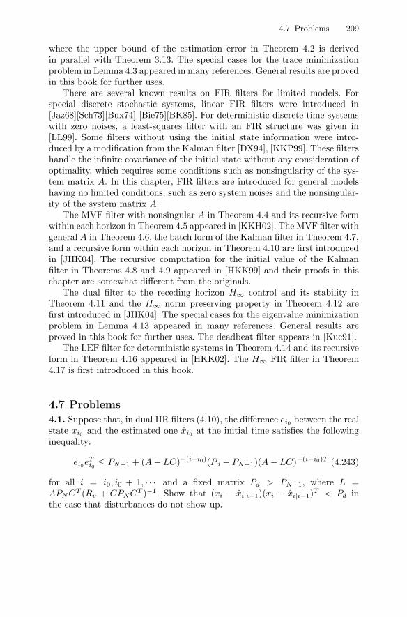
4.7 Problems 209

where the upper bound of the estimation error in Theorem 4.2 is derivedin parallel with Theorem 3.13. The special cases for the trace minimizationproblem in Lemma 4.3 appeared in many references. General results are provedin this book for further uses.

There are several known results on FIR filters for limited models. Forspecial discrete stochastic systems, linear FIR filters were introduced in[Jaz68][Sch73][Bux74] [Bie75][BK85]. For deterministic discrete-time systemswith zero noises, a least-squares filter with an FIR structure was given in[LL99]. Some filters without using the initial state information were intro-duced by a modification from the Kalman filter [DX94], [KKP99]. These filtershandle the infinite covariance of the initial state without any consideration ofoptimality, which requires some conditions such as nonsingularity of the sys-tem matrix A. In this chapter, FIR filters are introduced for general modelshaving no limited conditions, such as zero system noises and the nonsingular-ity of the system matrix A.

The MVF filter with nonsingular A in Theorem 4.4 and its recursive formwithin each horizon in Theorem 4.5 appeared in [KKH02]. The MVF filter withgeneral A in Theorem 4.6, the batch form of the Kalman filter in Theorem 4.7,and a recursive form within each horizon in Theorem 4.10 are first introducedin [JHK04]. The recursive computation for the initial value of the Kalmanfilter in Theorems 4.8 and 4.9 appeared in [HKK99] and their proofs in thischapter are somewhat different from the originals.

The dual filter to the receding horizon H∞ control and its stability inTheorem 4.11 and the H∞ norm preserving property in Theorem 4.12 arefirst introduced in [JHK04]. The special cases for the eigenvalue minimizationproblem in Lemma 4.13 appeared in many references. General results areproved in this book for further uses. The deadbeat filter appears in [Kuc91].

The LEF filter for deterministic systems in Theorem 4.14 and its recursiveform in Theorem 4.16 appeared in [HKK02]. The H∞ FIR filter in Theorem4.17 is first introduced in this book.

4.7 Problems

4.1. Suppose that, in dual IIR filters (4.10), the difference ei0 between the realstate xi0 and the estimated one xi0 at the initial time satisfies the followinginequality:

ei0eTi0 ≤ PN+1 + (A − LC)−(i−i0)(Pd − PN+1)(A − LC)−(i−i0)T (4.243)

for all i = i0, i0 + 1, · · · and a fixed matrix Pd > PN+1, where L =APNCT (Rv + CPNCT )−1. Show that (xi − xi|i−1)(xi − xi|i−1)T < Pd inthe case that disturbances do not show up.

210 4 Receding Horizon Filters

4.2. Consider the dual IIR filter (4.10).

(1) If Pi is the value of the optimal error variance when

Ji0,i= E[(xi − xi|i−1)T (xi − xi|i−1)|y1, y2, · · · , yi−1] (4.244)

is minimized, show that the inequality J∗i0,i+1 − J∗

i0,i ≤ 0 holds under thefollowing condition:

(A − LiC)Pi(A − LiC)T + GQwGT + LiRvLTi − Pi ≤ 0 (4.245)

where Li = APiCT (Rv + CPiC

T )−1 and J∗i0,i = min(4.244).

(2) Show that A − LiC should be Hurwitz in the inequality (4.245).(3) Show the following matrix inequality:[

I + C(ejwI − A)−1Li

](Rv + CPiC

T )[I + LT

i (e−jwI − AT )−1CT

]≥ Rv

4.3. Consider the following model:

xk+1 =[

0.9950 0.0998−0.0998 0.9950 + δk

]xk +

[0.10.1

]uk +

[1 01 0

]wk (4.246)

yk = [1 0]xk + vk (4.247)

where uncertain model parameter δk is defined in (4.146), Qw = 0.1I, andRv = 0.1. The initial state is taken as xT

0 = [2 2].

(1) Derive the steady-state Kalman filter and find its poles.(2) The control input is taken as a constant value by 1. Via simulation, com-

pare the transient response of the Kalman filter with that of the MVF filterwith horizon size 5. Repeat the simulations while changing the horizon sizeand discuss how the transient response of FIR filters is changed.

4.4. Assume that wk and vk are not uncorrelated in the system (4.1) and (4.2)and their covariances are given by

E

[wk

vk

] [wT

k vTk

]=[

Qw Swv

STwv Rv

](4.248)

Find out the MVF filter for the above case.

4.5. Let P1,i and P2,i be the solutions of two DREs

Pi+1 = APiAT − APiC

T [CPiCT + R]−1CPiA

T + Q (4.249)

with the same A,C and R matrices but different Q matrices Q1, Q2 and withinitial conditions P1(0) = P1 ≥ 0 and P2(0) = P2 ≥ 0 respectively. Show thatthe difference between the two solutions Pi = P2,i−P1,i satisfies the followingequation:

4.7 Problems 211

Pi+1 = AcPiATc − Λi(R + CP2,iC

T )Λi + Q (4.250)

where

Ac= A − AP1,iC

T (R + CP1,iCT )−1C

Λi= AcPiC

T (R + CP2,iCT )−1

Q= Q1 − Q2

4.6. Consider an MVF filter and an augmented linear model (4.27) withoutcontrol efforts

Yk−1 = CNxk + GNWk−1 + Vk−1 (4.251)

(1) Show that the minimum variance unbiased FIR filter xk|k−1 = HYk−1 forthe criterion

E[‖HYk−1 − xk‖2]

is determined so that each singular value σi

(H(GNQN GT

N + RN )12

)is

minimized. (σ1(·) ≥ σ2(·) ≥ · · · )(2) In order to handle the high risk more efficiently, we may employ the fol-

lowing criterion:

2γ2 log E exp(1

2γ2‖HYk−1 − xk‖2) (4.252)

Show that, in order to minimize the performance criterion (4.252), we haveonly to solve the following LMI:

minH

γ2 log det[

I γ−1MT

γ−1M I

]−1

subject to[

I γ−1MT

γ−1M I

]> 0

HCN = I

where M is defined by

M= H

[GN I

] [Qw 00 Rv

](4.253)

(3) Show the following inequality:

E[‖HYk−1 − xk‖2] ≤ 2γ2 log E exp(1

2γ2‖HYk−1 − xk‖2) (4.254)

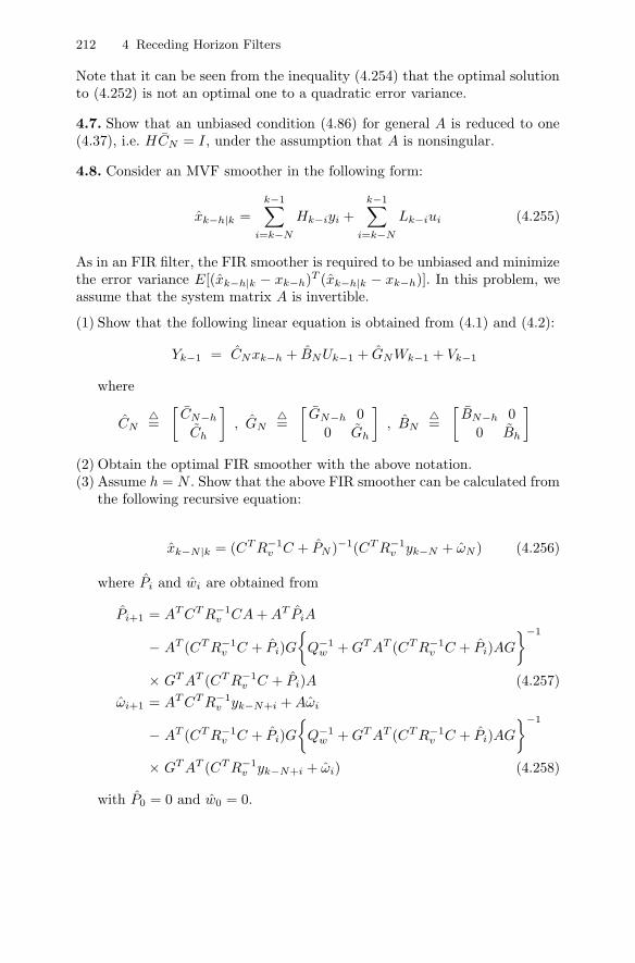
212 4 Receding Horizon Filters

Note that it can be seen from the inequality (4.254) that the optimal solutionto (4.252) is not an optimal one to a quadratic error variance.

4.7. Show that an unbiased condition (4.86) for general A is reduced to one(4.37), i.e. HCN = I, under the assumption that A is nonsingular.

4.8. Consider an MVF smoother in the following form:

xk−h|k =k−1∑

i=k−N

Hk−iyi +k−1∑

i=k−N

Lk−iui (4.255)

As in an FIR filter, the FIR smoother is required to be unbiased and minimizethe error variance E[(xk−h|k − xk−h)T (xk−h|k − xk−h)]. In this problem, weassume that the system matrix A is invertible.

(1) Show that the following linear equation is obtained from (4.1) and (4.2):

Yk−1 = CNxk−h + BNUk−1 + GNWk−1 + Vk−1

where

CN=[

CN−h

Ch

], GN

=[

GN−h 00 Gh

], BN

=[

BN−h 00 Bh

](2) Obtain the optimal FIR smoother with the above notation.(3) Assume h = N . Show that the above FIR smoother can be calculated from

the following recursive equation:

xk−N |k = (CT R−1v C + PN )−1(CT R−1

v yk−N + ωN ) (4.256)

where Pi and wi are obtained from

Pi+1 = AT CT R−1v CA + AT PiA

− AT (CT R−1v C + Pi)G

Q−1

w + GT AT (CT R−1v C + Pi)AG

−1

× GT AT (CT R−1v C + Pi)A (4.257)

ωi+1 = AT CT R−1v yk−N+i + Aωi

− AT (CT R−1v C + Pi)G

Q−1

w + GT AT (CT R−1v C + Pi)AG

−1

× GT AT (CT R−1v yk−N+i + ωi) (4.258)

with P0 = 0 and w0 = 0.

4.7 Problems 213

4.9. In MVF filters, we assume that the horizon size is greater than or equalto the system order. This assumption can be relaxed if the pseudo inverse isused as xk|k−1 = Ω+

N xk, where ΩN and xk are obtained from (4.68) and (4.72)respectively. Show that xk|k−1 = Ω+

N xk is the minimum norm solution to thefollowing performance criterion:

minxk

‖Yk−1 − BNUk−1 − CNxk‖2Ξ−1

N

(4.259)

where Yk−1, Uk−1, BN , CN and Ξk are defined as in (4.27) and (4.34).

4.10. Consider an autoregressive (AR) model signal given by

xi+1 =l∑

m=0

amxi−m + vi+1 (4.260)

where vi is an uncorrelated process noise with zero mean and variance σ andam is a finite sequence with ap−1 = 0.

(1) Represent the AR process (4.260) as a state-space model with Xi =[xi−l+1 ... x1]T .

(2) The above signal (4.260) is transmitted through l different channelsh1, ..., hl and measured with some noises such as

Yi = HXi + Wi

where

Yi =

⎡⎢⎣ y1,i

...yl,i

⎤⎥⎦ , H =

⎡⎢⎣h1

...hl

⎤⎥⎦ , Wi =

⎡⎢⎣w1,i

...wl,i

⎤⎥⎦as seen in Figure 4.10. Find out the MVF filter xk|k−1 = FYk−1 for thenoises Wi with zero means and E[WiW

Ti ] = Q.

4.11. In Section 4.3, two MVF filters (4.90) and (4.62) and (4.63) are derivedfor a general matrix A and a nonsingular matrix A respectively. Show that(4.62) and (4.63) can be obtained from (4.90) under the assumption of anonsingular matrix A.

4.12. Consider the following signal:

zi =ao,i√

2+

bo,i(−1)i

√2

+N−1∑k=1

[ak,i cos

(2πki

T

)+ bk,i sin

(2πki

T

)]+ vi (4.261)

where N is the number of harmonic components presented in zi, vi is the whiteGaussian measurement noise with mean 0 and variance σ2, and ak, bk; k =

214 4 Receding Horizon Filters

kx

lh

2h

1h

| 1ˆk kx −

1,kw

2,kw

,l kw

1,ky

2,ky

,l ky

kx

lh

2h

1h

| 1ˆk kx −

1,kw

2,kw

,l kw

1,ky

2,ky

,l ky

Fig. 4.10. Multi-channel optimal FIR filter

0, 1, 2, · · · , N−1 are the Fourier coefficients of the kth harmonic components.Then, the state model for the signal zi can be represented as

xi+1 = Axi (4.262)zi = Cxi + vi (4.263)

where

A =

⎡⎢⎢⎢⎢⎢⎣1 00 −1

Θ1

. . .ΘN−1

⎤⎥⎥⎥⎥⎥⎦Θk =

[cos kθ sin kθ− sin kθ cos kθ

]C =

[1√2

1√2

1 0 1 · · · 1 0]

where θ = 2πT . Here, the state xi is given by

xi =

⎡⎢⎢⎢⎢⎢⎢⎢⎢⎢⎣

x1,i

x2,i

x3,i

x4,i

...x2N−1,i

x2N,i

⎤⎥⎥⎥⎥⎥⎥⎥⎥⎥⎦=

⎡⎢⎢⎢⎢⎢⎢⎢⎢⎢⎣

a0

(−1)ib0

a1 cos θ + b1 sin θ−a1 sin θ + b1 cos θ

...aN−1 cos[(N − 1)θ] + bN−1 sin[(N − 1)θ]−aN−1 sin[(N − 1)θ] + bN−1 cos[(N − 1)θ]

⎤⎥⎥⎥⎥⎥⎥⎥⎥⎥⎦(1) Obtain the MVF filter.

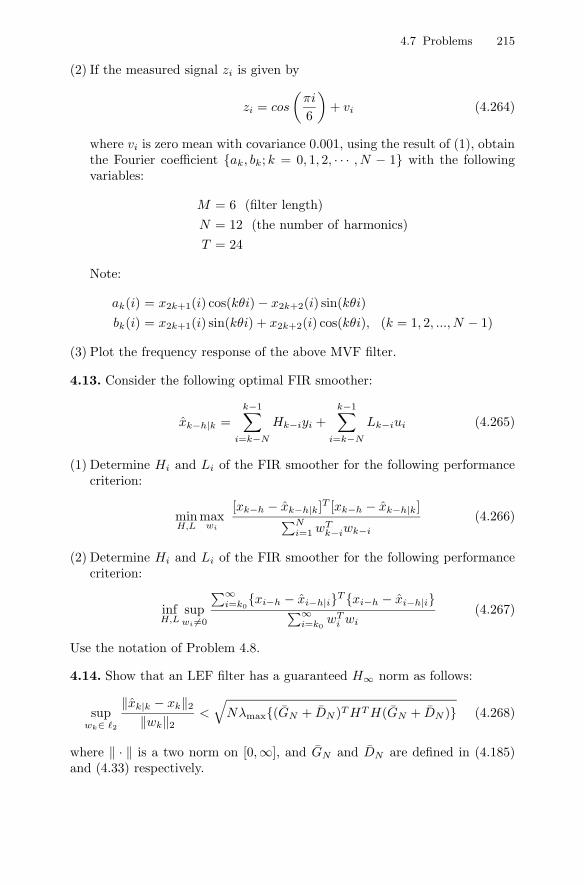
4.7 Problems 215

(2) If the measured signal zi is given by

zi = cos

(πi

6

)+ vi (4.264)

where vi is zero mean with covariance 0.001, using the result of (1), obtainthe Fourier coefficient ak, bk; k = 0, 1, 2, · · · , N − 1 with the followingvariables:

M = 6 (filter length)N = 12 (the number of harmonics)T = 24

Note:

ak(i) = x2k+1(i) cos(kθi) − x2k+2(i) sin(kθi)bk(i) = x2k+1(i) sin(kθi) + x2k+2(i) cos(kθi), (k = 1, 2, ..., N − 1)

(3) Plot the frequency response of the above MVF filter.

4.13. Consider the following optimal FIR smoother:

xk−h|k =k−1∑

i=k−N

Hk−iyi +k−1∑

i=k−N

Lk−iui (4.265)

(1) Determine Hi and Li of the FIR smoother for the following performancecriterion:

minH,L

maxwi

[xk−h − xk−h|k]T [xk−h − xk−h|k]∑Ni=1 wT

k−iwk−i

(4.266)

(2) Determine Hi and Li of the FIR smoother for the following performancecriterion:

infH,L

supwi =0

∑∞i=k0

xi−h − xi−h|iT xi−h − xi−h|i∑∞i=k0

wTi wi

(4.267)

Use the notation of Problem 4.8.

4.14. Show that an LEF filter has a guaranteed H∞ norm as follows:

supwk∈ 2

‖xk|k − xk‖2

‖wk‖2<√

Nλmax(GN + DN )T HT H(GN + DN ) (4.268)

where ‖ · ‖ is a two norm on [0,∞], and GN and DN are defined in (4.185)and (4.33) respectively.

216 4 Receding Horizon Filters

4.15. Derive an L2-E FIR filter again without a requirement of the nonsin-gularity of A.

4.16. Consider the linear discrete time-invariant state-space model as

xk+1 =[

0.9950 0.0998−0.0998 0.9950

]xk +

[11

]uk +

[0.10.1

]wk

yk =[1 1]xk + vk (4.269)

where the initial state is taken as xoT = [0 0] and the system noise covariance

Q is 0.01 and the measurement noise covariance R is 0.01.

(1) Compute the error covariance of the FIR filter and Kalman filter on round-off digits of fourth, third and second with horizon size 5.

(2) From your simulation result in (1), explain why the error covariance of anFIR filter is smaller than the error covariance of a Kalman filter.

5

Output Feedback Receding Horizon Controls

5.1 Introduction

In this chapter, it is assumed that the output can be measured and the inputis known. Controls that use only the measured output and the known controlare called output feedback controls, which are an important class of controls.There are different approaches for output feedback controls.

The first approach is a state-observer-based output feedback control. It canbe called a blind combination approach, where output feedback controls can beobtained by merely combining state feedback controls with state estimators.There exist many well-known state feedback controls, such as LQC in Chapter2 or LQ RHC in Chapter 3, and many state estimators, such as Luenburgerobservers for deterministic systems and Kalman filters for stochastic systemsin Chapter 2 or FIR filters in Chapter 4. This approach is easy to implement.However, it has no built-in optimality. It is noted that the stability of overalloutput feedback systems is determined by those of the controller and theobserver.

The second approach is a predictor-based output feedback control. It canbe called a predictor-based optimization approach. One can obtain predictorsfor the future states from measured outputs and known inputs and thesepredictors are considered in the performance criterion. The optimal controlfor linear systems turns out to be a function of the current estimated state.GPC can be approached this way and provided as output feedback controls,as seen in exercises.

The third approach is a global optimization approach. Usually, the opti-mal control may not provide the output feedback structure. Thus, we intro-duce controls with a built-in output feedback structure as a requirement. Theperformance criterion is optimized subject to controls with a finite memoryfeedback structure. Fortunately, the optimal control for linear systems is givenin the form of an output feedback control.

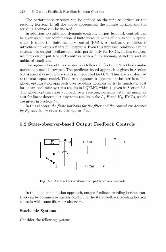
218 5 Output Feedback Receding Horizon Controls

The performance criterion can be defined on the infinite horizon or thereceding horizon. In all the above approaches, the infinite horizon and thereceding horizon can be utilized.

In addition to static and dynamic controls, output feedback controls canbe given as a linear combination of finite measurements of inputs and outputs,which is called the finite memory control (FMC). An unbiased condition isintroduced in various filters in Chapter 4. Even this unbiased condition can beextended to output feedback controls, particularly for FMCs. In this chapter,we focus on output feedback controls with a finite memory structure and anunbiased condition.

The organization of this chapter is as follows. In Section 5.2, a blind combi-nation approach is covered. The predictor-based approach is given in Section5.3. A special case of I/O systems is introduced for GPC. They are transformedto the state-space model. The direct approaches appeared in the exercises. Theglobal optimization approach over receding horizons with the quadratic costfor linear stochastic systems results in LQFMC, which is given in Section 5.5.The global optimization approach over receding horizons with the minimaxcost for linear deterministic systems results in the L2-E and H∞ FMCs, whichare given in Section 5.6.

In this chapter, the finite horizons for the filter and the control are denotedby Nf and Nc in order to distinguish them.

5.2 State-observer-based Output Feedback Controls

Fig. 5.1. State-observer-based output feedback controls

In the blind combination approach, output feedback receding horizon con-trols can be obtained by merely combining the state feedback receding horizoncontrols with some filters or observers.

Stochastic Systems

Consider the following system:

5.2 State-observer-based Output Feedback Controls 219

xi+1 = Axi + Bui + Gwi (5.1)yi = Cxi + vi (5.2)

where xi ∈ n, ui ∈ l and yi ∈ q are the state, the input, and the mea-surement respectively. At the initial time k0, the state xk0 is a random vari-able with a mean xk0 and a covariance Pk0 . The system noise wi ∈ p andthe measurement noise vi ∈ q are zero mean white Gaussian and mutuallyuncorrelated. The covariances of wi and vi are denoted by Qw and Rv respec-tively, which are assumed to be positive definite matrices. These noises areuncorrelated with the initial state xk0 .

The Kalmam filters are the most popular filters or observers for linearstochastic systems in Chapter 2. We can also use Kalman filters with frozengains or MVF filters in Chapter 4. For a typical example, combining a recedinghorizon LQ control in Chapter 3 with an MVF filter in Chapter 4 can be taken.Thus, we have

uk = −R−1BT [I + K1BR−1BT ]−1K1Axk|k−1 (5.3)

where xk|k−1 is obtained from

xk|k−1 = (CTNf

Ξ−1Nf

CNf)−1CT

NfΞ−1

Nf(Yk−1 − BNf

Uk−1) (5.4)

Here, Yk−1, Uk−1, CNf, BNf

and ΞNfare defined in (4.76), (4.77), (4.31),

(4.32) and (4.214) respectively and K1 is obtained from

Kj = AT Kj+1A − AT Ki+1B[R + BT Kj+1B]−1BT Kj+1A + Q

= AT Kj+1[I + BR−1BT Kj+1]−1A + Q

KNc= Qf

Note that it is assumed in (5.4) that A is invertible.This method is easy to implement. However, it has no optimality. The sta-

bility of the observer-based output feedback control for the stochastic systemcan be investigated such as in Section 5.5.4.

Deterministic Systems

Consider the following systems:

xi+1 = Axi + Bui + Bwwi (5.5)yi = Cxi + Cwwi (5.6)

where xi ∈ n, ui ∈ l, and yi ∈ q are the state, the input, and themeasurement respectively. Note that CwBT

w = 0.The most popular filters or observers are H∞ filters for the linear deter-

ministic systems in Chapter 2. We can also use H∞ filters with frozen gains orthe H∞ FIR filters in Chapter 4. For a typical example, combining a receding

220 5 Output Feedback Receding Horizon Controls

horizon H∞ control in Chapter 3 with an H∞ FIR filter in Chapter 4 can betaken. Thus, we have

uk = −R−1BT Λ−1k+1,k+Nc

Mk+1,k+NcAxk|k−1 (5.7)

where

Mj = AT Λ−1j+1Mj+1A + Q, j = 1, · · · , Nc − 1

MNc= Qf

Λj+1 = I + Mj+1(BR−1BT − γ−2BwR−1w BT

w)

xk|k−1 in (5.7) is calculated as

xk|k−1 = [FM + (CTNf

CNf)−1CT

Nf](Yk−1 − CT

NfUk−1)

where the columns of M is the basis of the null space of CTN and F is obtained

from the following LMI:

minF,X>0

γ∞

subject to⎡⎢⎢⎣−X XAu XBu 0

AuT X −X 0 S0

BuT X 0 −γ∞I 00 ST

0 0 −γ∞I

⎤⎥⎥⎦ < 0

Here, Au and Bu are defined in (4.227) and S0 = (GNf+ DNf

)T MT FT +(GNf

+ DNf)T ((CT

NfCNf

)−1CTNf

)T .The stability of the observer-based output feedback control for the deter-

ministic system can be investigated such as in Section 5.6.4.

5.3 Predictor-based Output Feedback Controls

For the predictor-based optimization approach, first a predictor is obtainedand then the optimization is carried out with a performance criterion basedon the predictor, as shown in Figure 5.2.

Stochastic Systems

In the system (5.1) and (5.2), the predictor estimates the future state us-ing the measurements and known inputs, and can be represented as

xk+i|k = x(k + i|y0, y1, · · · , yk, u0, u1 , · · · , uk, uk+1, · · · , uk+i−1) (5.8)

If stochastic noises are considered in plant models, then the predictor canbe expressed using the expectation

5.3 Predictor-based Output Feedback Controls 221

Fig. 5.2. Predictor-based output feedback control

xk+i|k = E

[x(k + i|y0, y1, · · · , yk, u0, u1, · · · , uk, uk+1, · · · , uk+i−1)

](5.9)

For the linear stochastic system (5.1) and (5.2), assume that xk|k is a filter ofxk. Then the predictor xk+i|k can be obtained:

xk+i+1|k = Axk+i|k + Buk+i|k (5.10)

where xk|k = xk and xk is a certain given filter.Thus, a performance criterion is as follows:

Nc−1∑j=0

[xT

k+j|kQxk+j|k + uTk+j|kRuk+j|k

]+ xT

k+Nc|kFxk+Nc|k (5.11)

Then, the solution to the problem (5.10) and (5.11) can be given by

uk = −R−1BT [I + K1BR−1BT ]−1K1Axk (5.12)

where Ki is given by

Ki = AT Ki+1A − AT Ki+1B[R + BT Ki+1B]−1BT Ki+1A + Q

= AT Ki+1[I + BR−1BT Ki+1]−1A + Q (5.13)

with the boundary condition

KNc= F (5.14)

Deterministic Systems

The predictor xk+i|k can be represented as

xk+i+1|k = Axk+i|k + Buk+i|k + Bwwk+i|k (5.15)

where xk|k = xk. The performance criterion is given by

222 5 Output Feedback Receding Horizon Controls

J(xk, uk+·|k, wk+·|k) =Nc−1∑j=0

[xT

k+j|kQxk+j|k + uTk+j|kRuk+j|k

− γ2wTk+j|kRwwk+j|k

]+xT

k+Nc|kQf xk+Nc|k (5.16)

Then, the solution to the problem (5.15) and (5.16) can be given by

uk = −R−1BT Λ−1k+1,k+Nc

Mk+1,k+NcAxk

where

Mj = AT Λ−1j+1Mj+1A + Q

MNc= Qf

Λj+1 = I + Mj+1(BR−1BT − γ−2BwR−1w BT

w)

for j = 1, · · · , Nc − 1.For stochastic and deterministic systems, stabilities of the predictor-based

output feedback controls are determined according to what kinds of filters areused.

5.4 A Special Case of Input–Output Systems of GeneralPredictive Control

In addition to the stochastic state-space system (5.1) and (5.2), GPC has usedthe following CARIMA model:

A(q−1)yi = B(q−1)ui−1 + C(q−1)wi (5.17)

where A(q−1) and B(q−1) are given in (3.195) and (3.196) and C(q−1) is givenas follows:

C(q−1) = 1 + c1q−1 + · · · + cnq−n (5.18)

It is noted that the C(q−1) can often be

1 + c1q−1 + · · · + cpq

−p, p ≤ n (5.19)

The CARIMA model (5.17) can be rewritten as

A(q−1)yi = B(q−1)ui + C(q−1)wi (5.20)

where

B(q−1) = b1q−1 + b2q

−2 · · · + bnq−n+1

From (5.20) we can obtain

5.4 A Special Case of Input–Output Systems of General Predictive Control 223

A(q−1)(yi − wi) = B(q−1)ui + [C(q−1) − A(q−1)]wi (5.21)

where

C(q−1) − A(q−1) = (c1 − a1)q−1 + · · · + (cn − an)q−n (5.22)

Therefore, (5.21) has a similar structure to (3.200), such as

xi+1 = Axi + Bui + Dwwi

yi = Cxi + wi (5.23)

where A,B,C, and Dw are given by

A =

⎡⎢⎢⎢⎢⎢⎣−a1 1 0 · · · 0−a2 0 1 · · · 0

......

.... . .

...−an−1 0 0 · · · 1−an 0 0 · · · 0

⎤⎥⎥⎥⎥⎥⎦ , B =

⎡⎢⎢⎢⎢⎢⎣b1

b2

...bn−1

bn

⎤⎥⎥⎥⎥⎥⎦ (5.24)

C =[1 0 0 · · · 0

], Dw =

⎡⎢⎣ c1 − a1

...cn − an

⎤⎥⎦Stochastic Systems

In (5.23), wi is a zero mean white noise with a covariance qw. It is notedthat the system noise and measurement noise are correlated as seen in (5.23).The performance criterion for (5.17) can be given as

E

⎧⎨⎩Nc∑j=1

[q(yk+j − yr

k+j)2 + r(uk+j−1)2|[ks,k]

]⎫⎬⎭+E

⎧⎨⎩Np∑

j=Nc+1

qf (yk+j − yrk+j)

2|[ks,k]

⎫⎬⎭ (5.25)

where uk+Nc= ... = uk+Np−1 = 0. Expectation is taken under the con-

dition that the measurement data of yi and ui on [ks, k] are given. Theperformance index (5.25) can be changed to

Nc∑j=1

[q(yk+j|k − yr

k+j)2 + r(uk+j−1)2

]+

Np∑j=Nc+1

qf (yk+j|k − yrk+j)

2 (5.26)

224 5 Output Feedback Receding Horizon Controls

We can have predictors

xk+j+1|k = Axk+j|k + Buk+j|k j ≥ 1 (5.27)yk+j|k = Cxk+j|k (5.28)

But, if j = 0, the system noise and measurement noise are correlated. So,by using the result of Problem 2.15, we can change the correlated state-spacemodel (5.23) into the uncorrelated state-space model:

xi+1 = Axi + Bui + Dwyi

yi = Cxi + wi (5.29)

where A = A − DwC. Therefore, if j = 0, then we can have a predictor

xk+1|k = Axk|k + Buk + Dwyk (5.30)

Using (5.27), (5.28), and (5.30), we can obtain

yk+j|k = CAj−1Axk|k +j−1∑i=0

CAj−i−1Buk+i + CAj−1Dwyk (5.31)

where xk|k = xk|k could be a starting point.GPC can be obtained from the predictor (5.31) and the performance cri-

terion (5.26). The GPC can be given similar to (3.329) as follows:

Uk =[W

TQW + W

T

f QfW f + R]−1

WTQ[Y r

k − V xk|k − Nyk

]+ W

T

f Qf

[Y r

k+Nc− V f xk|k − Nfyk

](5.32)

where

Y rk =

⎡⎢⎣ yrk+1...

yrk+Nc

⎤⎥⎦ , V =

⎡⎢⎢⎢⎣CA

CAA...

CANc−1A

⎤⎥⎥⎥⎦ , Uk =

⎡⎢⎣ uk

...uk+Nc−1

⎤⎥⎦

Y rk+Nc

=

⎡⎢⎣ yrk+Nc+1

...yr

k+Np

⎤⎥⎦ , V f =

⎡⎢⎣ CANcA...

CANp−1A

⎤⎥⎦

W =

⎡⎢⎣ CB · · · 0...

. . ....

CANc−1B · · · CB

⎤⎥⎦ , W f =

⎡⎢⎣ CANcB · · · CAB...

. . ....

CANp−1B · · · CANp−NcB

⎤⎥⎦Q =

[diag(

Nc︷ ︸︸ ︷q q · · · q)

], Qf =

[diag(

Np−Nc︷ ︸︸ ︷qf qf · · · qf )

]

5.4 A Special Case of Input–Output Systems of General Predictive Control 225

R =[diag(

Nc︷ ︸︸ ︷r r · · · r)

], N =

⎡⎢⎢⎢⎣CDw

CADw

...CANc−1Dw

⎤⎥⎥⎥⎦ , Nf =

⎡⎢⎣ CANcDw

...CANp−1Dw

⎤⎥⎦Therefore, the GPC uk is given by

uk =[I 0 · · · 0

] [W

TQW + W

T

f QfW f + R]−1

WTQ

×[Y r

k − V xk|k − Nyk

]+ W

T

f Qf

[Y r

k+Nc− V f xk|k − Nfyk

](5.33)

A starting point xk|k can be obtained from an FIR filter:

xk|k =k∑

i=k−N

Hk−iyi +k−1∑

i=k−N

Lk−iui (5.34)

where Hk−i and Lk−i can be obtained similarly as in Chapter 4.

Deterministic Systems

We assume wi in (5.17) is a deterministic disturbance. We can have predictors

xk+j+1|k = Axk+j|k + Buk+j|k + Dwwk+j|k, j ≥ 1 (5.35)yk+j|k = Cxk+j|k + wk+j|k (5.36)

where a filter xk+1|k could be a starting point. From now on, uk+j|k andwk+j|k will be used as uk+j and wk+j respectively. We consider the followingperformance criterion:

Nc∑j=1

[q(yk+j − yr

k+j)2 + r(uk+j−1)2 − γ(wk+j−1)2

]+

Np∑j=Nc+1

qf (yk+j − yrk+j)

2 (5.37)

where uk+Nc= ... = uk+Np

= 0 and wk+Nc= ... = wk+Np

= 0. From thestate-space model (5.23), we have

yk+j = CAj xk|k +j−1∑i=0

CAj−i−1Buk+i +j−1∑i=0

CAj−i−1Dwk+i

+wk+j (5.38)

where xk|k = xk|k could be a starting point. The performance index (5.37)can be represented by

226 5 Output Feedback Receding Horizon Controls

J(xk,Uk,Wk) =[Y r

k − V xk|k − WUk − HWk

]TQ[Y r

k − V xk|k − WUk

− HWk]UTk RUk − WT

k ΓWk + [Y rk+Nc

− Vf xk|k − WfUk

− HfWk]T Qf

[Y r

k+Nc− Vf xk|k − WfUk − HfWk

](5.39)

where

Y rk =

⎡⎢⎣ yrk+1...

yrk+Nc

⎤⎥⎦ , V =

⎡⎢⎣ CA...

CANc

⎤⎥⎦ , Uk =

⎡⎢⎣ uk

...uk+Nc−1

⎤⎥⎦

Y rk+Nc

=

⎡⎢⎣ yrk+Nc+1

...yr

k+Np

⎤⎥⎦ , Vf =

⎡⎢⎣ CANc+1

...CANp

⎤⎥⎦ , Wk =

⎡⎢⎣ wk

...wk+Nc−1

⎤⎥⎦

W =

⎡⎢⎣ CB · · · 0...

. . ....

CANc−1B · · · CB

⎤⎥⎦ , Wf =

⎡⎢⎣ CANcB · · · CAB...

. . ....

CANp−1B · · · CANp−NcB

⎤⎥⎦R =

[diag(

Nc︷ ︸︸ ︷r r · · · r)

], Γ =

[diag(

Nc︷ ︸︸ ︷γ γ · · · γ)

]Qf =

[diag(

Np−Nc︷ ︸︸ ︷qf qf · · · qf )

], Q =

[diag(

Nc︷ ︸︸ ︷q q · · · q)

]

H =

⎡⎢⎢⎢⎢⎢⎣CDw I 0 · · · 0

CADw CDw I · · · 0...

. . . . . . . . ....

CANc−2Dw · · · · · · · · · ICANc−1Dw · · · · · · · · · CDw

⎤⎥⎥⎥⎥⎥⎦Hf =

⎡⎢⎣ CANcDw · · · CAB...

. . ....

CANp−1B · · · CANp−NcB

⎤⎥⎦If we compare (3.332) and (5.39), the condition that the solution to the saddlepoint exists is

HT QH − Γ + HTf QfHf < 0 (5.40)

the maximizing disturbance W ∗k is given by

W ∗k = V−1

1 V2 (5.41)

where

V1 = HT QH − Γ + HTf QfHf

V2 = HT Q[Y r

k − V xk|k − WUk

]+ HT

f Qf

[Y r

k+Nc− Vf xk|k − WfUk

]

5.5 Finite Memory Control Based on Minimum Criterion 227

and the optimal control vector U∗k is given by

U∗k = −P−1

1 P2 (5.42)

where

P1 = −(HT QW + HTf QfWf )TV−1

1 (HT QW + HTf QfWf ) + WT QW

+ RN + WTf QfWf

P2 = (HT QW + HTf QfWf )TV−1

1 [HT Q(Y rk − V xk|k)

+ HTf Qf (Y r

k+Nc− Vf xk|k)] − WT Q(Y r

k − V xk|k) − WTf Qf (Y r

k+Nc− Vf xk|k)

Therefore, the GPC uk is given by

uk = −[I 0 · · · 0

]P−1

1 P2 (5.43)

A starting point xk|k can be also obtained similarly as in an FIR filter (5.34).

5.5 Finite Memory Control Based on MinimumCriterion

5.5.1 Finite Memory Control and Unbiased Condition

Finite Memory Control

Output feedback controls with a finite memory structure can be representedusing measurements and inputs during a filter horizon [k − Nf , k] as

uk =k−1∑

i=k−Nf

Hk−iyi +k−1∑

i=k−Nf

Lk−iui (5.44)

where Hk−j and Lk−j are gain matrices with respect to yi and ui respectively.The control (5.44) can be represented in a simpler matrix form:

uk = HYk−1 + LUk−1 (5.45)

where H, L, Yk−1, and Uk−1 are defined as

H= [HNf

HNf−1 · · · H1] (5.46)

L= [LNf

LNf−1 · · · L1] (5.47)

Yk−1= [yT

k−NfyT

k−Nf+1 · · · yTk−1]

T (5.48)

Uk−1= [uT

k−NfuT

k−Nf+1 · · · uTk−1]

T (5.49)

Controls of the type (5.44) are visualized in Figure 5.3 and will be obtained

228 5 Output Feedback Receding Horizon Controls

Fig. 5.3. Block diagram of FMC

from a performance criterion on the finite horizon. To this end, we introduceintermediate controls on the finite horizon [k, k + Nc]. Intermediate outputfeedback controls with the finite memory structure can be represented usingmeasurements and inputs during a filter horizon [k − Nf + j, k + j] as

uk+j =k+j−1∑

i=k+j−Nf

H(j)k+j−iyi +

k+j−1∑i=k+j−Nf

L(j)k+j−iui (5.50)

where the gains H(j)· and L

(j)· may be dependent on j, and xk+j is the trajec-

tory generated from uk+j . Note that even though the control (5.50) uses thefinite measured outputs and inputs on the recent time interval as FIR filters,this is not of the FIR form, since controls appear on both sides of (5.50).So this kind of the control will be called an output feedback finite memorycontrol, or simply an FMC rather than an FIR control.

The FMC can be expressed as a linear function of the finite inputs Yk−1

and inputs Uk−1 on the horizon [k − Nf k] as follows:

uk+j = H(j)Yk+j−1 + L(j)Uk+j−1 (5.51)

where H(j), L(j), Yk+j−1, Uk+j−1 are defined as

5.5 Finite Memory Control Based on Minimum Criterion 229

H(j) = [H(j)

NfH

(j)Nf−1 · · · H

(j)1 ] (5.52)

L(j) = [L(j)

NfL

(j)Nf−1 · · · L

(j)1 ] (5.53)

Yk+j−1= [yT

k+j−NfyT

k+j−Nf+1 · · · yTk+j−1]

T (5.54)

Uk+j−1= [uT

k+j−NfuT

k+j−Nf+1 · · · uTk+j−1]

T (5.55)

It is a general rule of thumb that the FIR systems are robust against tem-porary modelling uncertainties or round-off errors. Therefore, the FMC mayhave such properties due to the finite memory structure.

Unbiased Condition

We start off from the case that the system matrix A is nonsingular and thenproceed to the case of the general matrix A in the next section.

As in FIR filters in Chapter 4, we are interested in the measured outputyk and the input uk on the finite recent horizon, from which the system (5.1)and (5.2) is represented as

Yk+j−1 = CNfxk+j + BNf

Uk+j−1 + GNfWk+j−1 + Vk+j−1 (5.56)

where Wk+j and Vk+j are given by

Wk+j= [wT

k+j−NfwT

k+j−Nf+1 · · · wTk+j−1]

T (5.57)

Vk+j= [vT

k+j−NfvT

k+j−Nf+1 · · · vTk+j−1]

T (5.58)

and CNf, BNf

, and GNfare obtained from (4.31), (4.32), and (4.33) respec-

tively.Combining (5.51) and (5.56) yields

uk+j = H(CNfxk+j + BNf

Uk+j−1 + GNfWk+j−1 + Vk+j−1)

+ LUk+j−1 (5.59)

If we assume that the full information of the state is available, then thedesirable control is represented in the form of a state feedback control

u∗k+j = −Kj+1xk+j (5.60)

where 0 ≤ j ≤ Nf − 1 and Kj+1 can be chosen to be optimized for a certainperformance criterion. It is desirable that the intermediate FMC (5.59) cantrack the state feedback control (5.60) on the average. Since any output feed-back control cannot be better in view of performance than the optimal statefeedback control, it is desirable that the control (5.59) should be unbiased fromthe optimal state feedback control (5.60). Thus, we require a constraint thatthe control (5.59) must be unbiased from the desired state feedback control(5.60) as

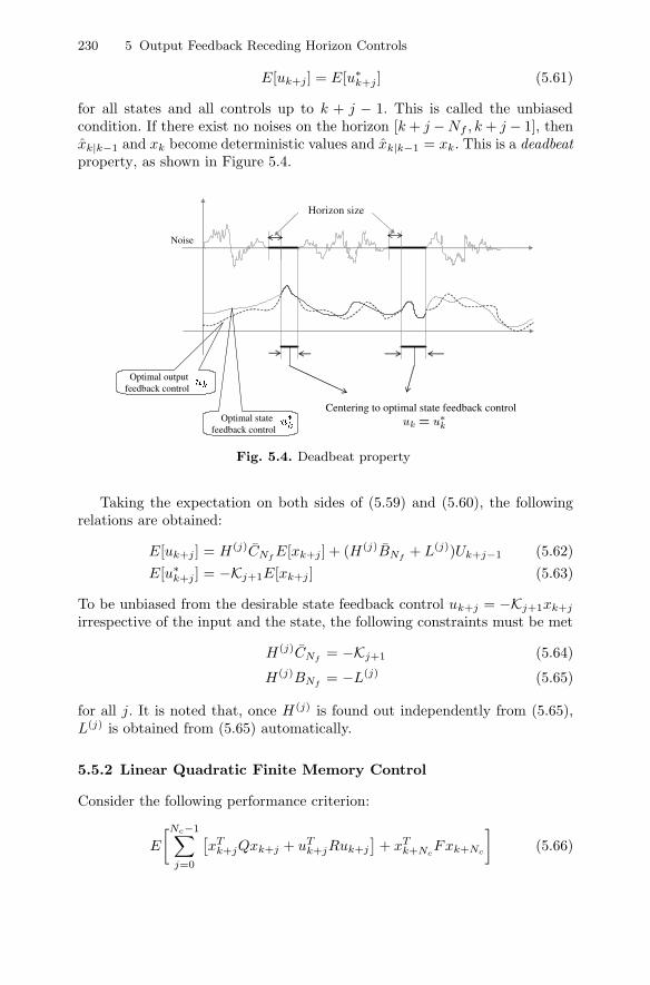
230 5 Output Feedback Receding Horizon Controls

E[uk+j ] = E[u∗k+j ] (5.61)

for all states and all controls up to k + j − 1. This is called the unbiasedcondition. If there exist no noises on the horizon [k + j −Nf , k + j − 1], thenxk|k−1 and xk become deterministic values and xk|k−1 = xk. This is a deadbeatproperty, as shown in Figure 5.4.

Optimal output feedback control

Centering to optimal state feedback control

Noise

Horizon size

Optimal state feedback control

Fig. 5.4. Deadbeat property

Taking the expectation on both sides of (5.59) and (5.60), the followingrelations are obtained:

E[uk+j ] = H(j)CNfE[xk+j ] + (H(j)BNf

+ L(j))Uk+j−1 (5.62)E[u∗

k+j ] = −Kj+1E[xk+j ] (5.63)

To be unbiased from the desirable state feedback control uk+j = −Kj+1xk+j

irrespective of the input and the state, the following constraints must be met

H(j)CNf= −Kj+1 (5.64)

H(j)BNf= −L(j) (5.65)

for all j. It is noted that, once H (j) is found out independently from (5.65),L(j) is obtained from (5.65) automatically.

5.5.2 Linear Quadratic Finite Memory Control

Consider the following performance criterion:

E

[Nc−1∑j=0

[xT

k+jQxk+j + uTk+jRuk+j

]+ xT

k+NcFxk+Nc

](5.66)

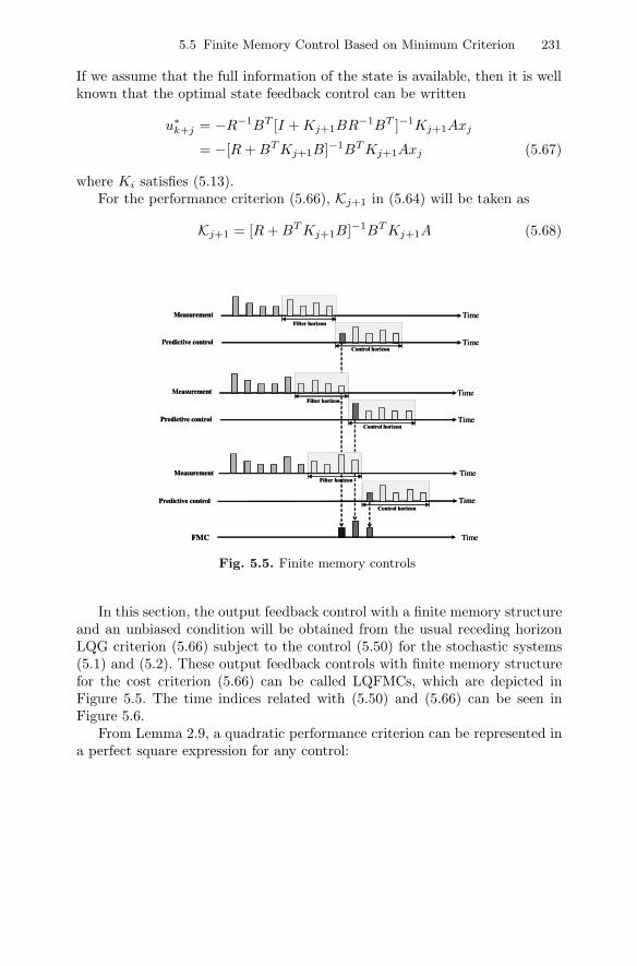
5.5 Finite Memory Control Based on Minimum Criterion 231

If we assume that the full information of the state is available, then it is wellknown that the optimal state feedback control can be written

u∗k+j = −R−1BT [I + Kj+1BR−1BT ]−1Kj+1Axj

= −[R + BT Kj+1B]−1BT Kj+1Axj (5.67)

where Ki satisfies (5.13).For the performance criterion (5.66), Kj+1 in (5.64) will be taken as

Kj+1 = [R + BT Kj+1B]−1BT Kj+1A (5.68)

FMC Time

Predictive control

MeasurementFilter horizon

Control horizon

Time

Time

Predictive control

MeasurementFilter horizon

Control horizon

Time

Time

Predictive control

MeasurementFilter horizon

Control horizon

Time

Time

FMC Time

Predictive control

MeasurementFilter horizon

Control horizon

Time

Time

Predictive control

MeasurementFilter horizon

Control horizon

Time

Time

Predictive control

MeasurementFilter horizon

Control horizon

Time

Time

Fig. 5.5. Finite memory controls

In this section, the output feedback control with a finite memory structureand an unbiased condition will be obtained from the usual receding horizonLQG criterion (5.66) subject to the control (5.50) for the stochastic systems(5.1) and (5.2). These output feedback controls with finite memory structurefor the cost criterion (5.66) can be called LQFMCs, which are depicted inFigure 5.5. The time indices related with (5.50) and (5.66) can be seen inFigure 5.6.

From Lemma 2.9, a quadratic performance criterion can be represented ina perfect square expression for any control:

232 5 Output Feedback Receding Horizon Controls

Fig. 5.6. Time variables for LQFMC

E

[Nc−1∑j=0

[xT

k+jQxk+j + uTk+jRuk+j

]+ xT

k+NcFxk+Nc

]

= E

[Nc−1∑j=0

−Kj+1xk+j + uk+jT Rj−Kj+1xk+j + uk+j]

+ tr[Nc−1∑

j=0

Kj+1GQwGT]+ E

[xT

k K0xk

](5.69)

where Rj= [R + BT Kj+1B], Kj+1 is defined in (5.68), and Kj+1 is the

solution to Riccati Equation (5.13).It is noted that the result of Lemma 2.9 holds for any inputs. By using

Lemma 2.9, the performance criterion can be changed to the following form:

HB = arg minH(0),··· ,H(Nc−1)

E

[Nc−1∑j=0

[xT

k+jQxk+j + uTk+jRuk+j

]+ xT

k+NcFxk+Nc

]

= arg minH(0),··· ,H(Nc−1)

E

[Nc−1∑j=0

Kj+1xk+j + uk+j

TRj

Kj+1xk+j + uk+j

]

+ tr[Nc−1∑

j=0

Kj+1GQwGT]+ E

[xT

k K0xk

](5.70)

It can be seen that the last two terms in (5.70) do not depend on a controlgain H(j). We have only to minimize the first term in (5.70) in order to obtainthe solution.

Since, under the unbiasedness constraint, the following equation is ob-tained:

5.5 Finite Memory Control Based on Minimum Criterion 233

uk+j + Kj+1xk+j = H(j)GNfWk+j−1 + H(j)Vk+j−1 (5.71)

the first term in (5.70) is obtained as

E

[Kj+1xk+j + uk+j

TRj

Kj+1xk+j + uk+j

]= E

[H(j)GNf

Wk+j−1 + H(j)Vk+j−1

TRj

H(j)GNf

Wk+j−1 + H(j)Vk+j−1

]= tr

[R

12j H(j)GNf

QNfGT

NfH(j)T R

12j + R

12j H(j)RNf

H(j)T R12j

](5.72)

The objective now is to obtain the optimal gain matrix H(j)B , subject to the

unbiasedness constraint (5.65), in such a way that the cost function (5.72) hasa minimum variance as follows:

H(j)B = arg min

H(j)tr[R

12j H(j)GNf

QNfGT

NfH(j)T R

12j

+ R12j H(j)RNf

H(j)T R12j

](5.73)

subject toH(j)CNf

= −Kj+1 (5.74)

where

QNf=[diag(

Nf︷ ︸︸ ︷Qw Qw · · · Qw)

]and RNf

=[diag(

Nf︷ ︸︸ ︷Rv Rv · · · Rv)

](5.75)

By using the result of Lemma 4.3, the solution to the optimization problem(5.73) and (5.74) can be obtained according to the following correspondences:

A ←− GNf

B ←− OC ←− QNf

D ←− RNf

E ←− CNf

F ←− −R12j Kj+1

H ←− R12j H(j)

(5.76)

L(j) is determined from (5.65). It follows finally that

uk+j = −H(j)Yk+j−1 + L(j)Uk+j−1

= −Kj+1(CTNf

Ξ−1Nf

CNf)−1CT

NfΞ−1

Nf(Yk+j−1 − BNf

Uk+j−1) (5.77)

If j is fixed to zero in (5.77), then we obtain the optimal solution for LQFMCin the following theorem.

234 5 Output Feedback Receding Horizon Controls

Theorem 5.1. When A,C is observable and Nf ≥ no, the LQFMC uk

is given as follows:

uk = −K1(CTNf

Ξ−1Nf

CNf)−1CT

NfΞ−1

Nf(Yk−1 − BNf

Uk−1) (5.78)

in the case that A is nonsingular. Yk−1, Uk−1, CNf, BNf

, ΞNf, and K1 are

given by (5.54), (5.55), (4.31), (4.32), (4.214), and (5.68) respectively.

The dimension of ΞNfin (5.78) may be large. So a numerical error during

inverting the matrix can happen. To avoid the handling of the large matrix,the optimal gain matrix for a nonsingular A can be obtained from the followingrecursive equations:

HB = −[R + BT K1B]−1BT K1AΩ−1Nf

ΨNf(5.79)

where ΩNfis defined as CT

NfΞ−1

NfCNf

as in Chapter 4 and is written recursivelyas

Ωi+1 = [I + A−T (Ωi + CT R−1v C)A−1GQwGT ]−1A−T (Ωi + CT R−1

v C)A−1

with Ω0 = 0. We define

Ψi+1= CT

i+1Ξ−1i+1 = [I + A−T (Ωi + CT R−1

v C)A−1GQwGT ]−1A−T

×[

Ci

C

]T [Ξi 00 Rv

]−1

(5.80)

with Ψ0 = 0 and then recursive equations for Ψi can be easily derived fromthe structure of the matrix ΞNf

in (5.78) as follows:

Ψi+1 = [I + A−T (Ωi + CT R−1v C)A−1GQwGT ]−1A−T

[Ψi CT R−1

v

](5.81)

which is left as an exercise. From Theorem 5.1, it can be known that theLQFMC uk (5.78) processes the finite measurements and inputs on the horizon[k − Nf , k] linearly and has the properties of unbiasedness from the optimalstate feedback control by design. Note that the optimal gain matrix HB (5.79)requires a computation only on the interval [0, Nf ] once and is time-invariantfor all horizons. This means that the LQFMC is time-invariant. The LQFMCmay be robust against temporary modelling uncertainties or round-off errorsdue to the finite memory structure.

So far, we have derived the LQFMC in a closed form. Besides the analyticalform, the LQFMC can be represented in LMI form to get a numerical solution.

First, from the unbiased condition HCNf= −K1, the control gain H of

the LQFMC can be parameterized as

H = FMT + H0 (5.82)

where H0 = −K1(CTNf

CNf)−1CT

Nfand the columns of M consist of the basis

of the null space of CTNf

. Let us introduce a matrix variable W such that

5.5 Finite Memory Control Based on Minimum Criterion 235

W > R12 HGNf

QNfGT

NfHR

12 + R

12 HRNf

HT R12 (5.83)

where R is given by

R = R + BT K1B

Thus, from (5.83) we have

minW,F

γ (5.84)

subject to

tr(W ) < γ

[W R

12 (FMT + H0)

(FMT + H0)T R12 (GNf

QNfGT

Nf+ RNf

)−1

]> 0 (5.85)

From the optimal H we obtain L = −HBNf.

5.5.3∗ Linear Quadratic Finite Memory Control with General A

Now we turn to the case where the system matrix A is general.The system (5.1) and (5.2) will be represented in a batch form on the time

interval [k+j−Nf , k+j] called the horizon. On the horizon [k+j−Nf , k+j],measurements are expressed in terms of the state xk+j at the time k + j andinputs on [k + j − Nf , k + j] as follows:

Yk+j−1 = CNfxk+j−Nf

+ BNfUk+j−1 + GNf

Wk+j−1 + Vk+j−1 (5.86)

where

Yk+j−1= [yT

k+j−NfyT

k+j−Nf+1 · · · yTk+j−1]

T (5.87)

Uk+j−1= [uT

k+j−NfuT

k+j−Nf+1 · · · uTk+j−1]

T (5.88)

Wk+j−1= [wT

k+j−NfwT

k+j−Nf+1 · · · wTk+j−1]

T (5.89)

Vk+j−1= [vT

k+j−NfvT

k+j−Nf+1 · · · vTk+j−1]

T

and CNf, BNf

, and GNfare obtained from (4.78), (4.79), and (4.80) respec-

tively. The noise term GNfWj−1 + Vj−1 in (4.75) can be shown to be zero

mean with a covariance ΠN given by

ΠNf= GNf

QNfGT

Nf+ RNf

(5.90)

where QNfand RNf

are given in (5.75).

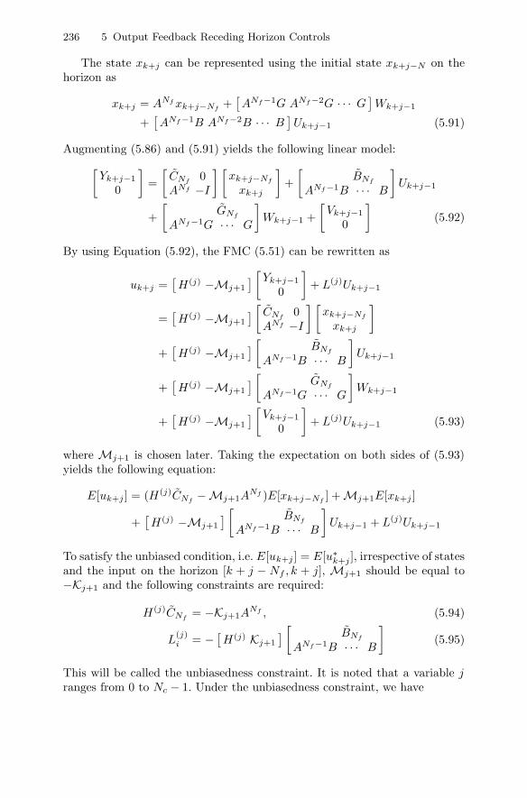
236 5 Output Feedback Receding Horizon Controls

The state xk+j can be represented using the initial state xk+j−N on thehorizon as

xk+j = ANf xk+j−Nf+[ANf−1G ANf−2G · · · G

]Wk+j−1

+[ANf−1B ANf−2B · · · B

]Uk+j−1 (5.91)

Augmenting (5.86) and (5.91) yields the following linear model:[Yk+j−1

0

]=[

CNf0

ANf −I

] [xk+j−Nf

xk+j

]+[

BNf

ANf−1B · · · B

]Uk+j−1

+[

GNf

ANf−1G · · · G

]Wk+j−1 +

[Vk+j−1

0

](5.92)

By using Equation (5.92), the FMC (5.51) can be rewritten as

uk+j =[H(j) −Mj+1

] [Yk+j−1

0

]+ L(j)Uk+j−1

=[H(j) −Mj+1

] [ CNf0

ANf −I

] [xk+j−Nf

xk+j

]+[H(j) −Mj+1

] [ BNf

ANf−1B · · · B

]Uk+j−1

+[H(j) −Mj+1

] [ GNf

ANf−1G · · · G

]Wk+j−1

+[H(j) −Mj+1

] [Vk+j−1

0

]+ L(j)Uk+j−1 (5.93)

where Mj+1 is chosen later. Taking the expectation on both sides of (5.93)yields the following equation:

E[uk+j ] = (H(j)CNf−Mj+1A

Nf )E[xk+j−Nf] + Mj+1E[xk+j ]

+[H(j) −Mj+1

] [ BNf

ANf−1B · · · B

]Uk+j−1 + L(j)Uk+j−1

To satisfy the unbiased condition, i.e. E[uk+j ] = E[u∗k+j ], irrespective of states

and the input on the horizon [k + j − Nf , k + j], Mj+1 should be equal to−Kj+1 and the following constraints are required:

H(j)CNf= −Kj+1A

Nf , (5.94)

L(j)i = −

[H(j) Kj+1

] [ BNf

ANf−1B · · · B

](5.95)

This will be called the unbiasedness constraint. It is noted that a variable jranges from 0 to Nc − 1. Under the unbiasedness constraint, we have

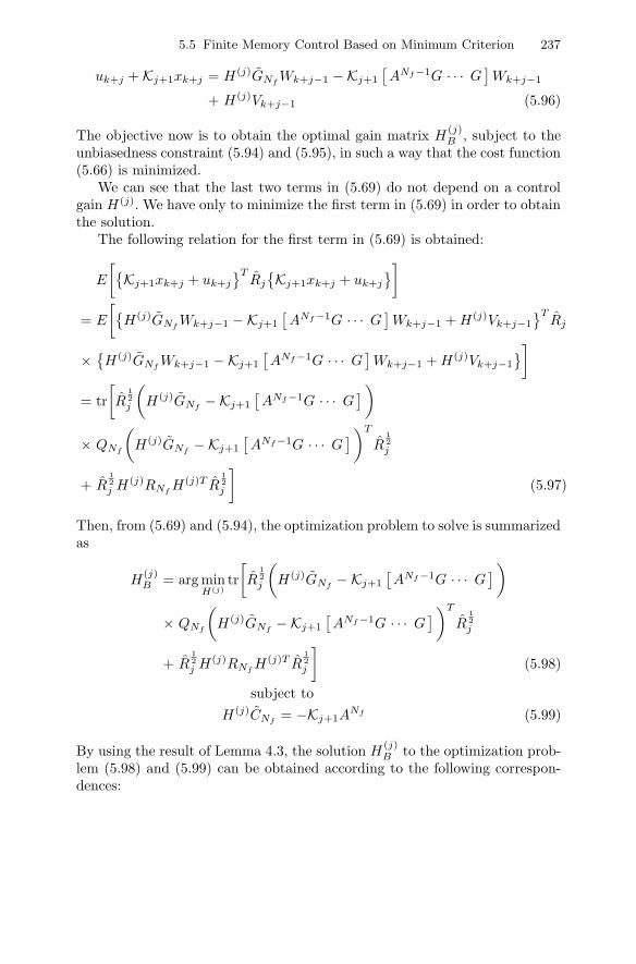
5.5 Finite Memory Control Based on Minimum Criterion 237

uk+j + Kj+1xk+j = H(j)GNfWk+j−1 −Kj+1

[ANf−1G · · · G

]Wk+j−1

+ H(j)Vk+j−1 (5.96)

The objective now is to obtain the optimal gain matrix H(j)B , subject to the

unbiasedness constraint (5.94) and (5.95), in such a way that the cost function(5.66) is minimized.

We can see that the last two terms in (5.69) do not depend on a controlgain H(j). We have only to minimize the first term in (5.69) in order to obtainthe solution.

The following relation for the first term in (5.69) is obtained:

E

[Kj+1xk+j + uk+j

TRj

Kj+1xk+j + uk+j

]= E

[H(j)GNf

Wk+j−1 −Kj+1

[ANf−1G · · · G

]Wk+j−1 + H(j)Vk+j−1

TRj

×H(j)GNf

Wk+j−1 −Kj+1

[ANf−1G · · · G

]Wk+j−1 + H(j)Vk+j−1

]= tr

[R

12j

(H(j)GNf

−Kj+1

[ANf−1G · · · G

])× QNf

(H(j)GNf

−Kj+1

[ANf−1G · · · G

])T

R12j

+ R12j H(j)RNf

H(j)T R12j

](5.97)

Then, from (5.69) and (5.94), the optimization problem to solve is summarizedas

H(j)B = arg min

H(j)tr[R

12j

(H(j)GNf

−Kj+1

[ANf−1G · · · G

])× QNf

(H(j)GNf

−Kj+1

[ANf−1G · · · G

])T

R12j

+ R12j H(j)RNf

H(j)T R12j

](5.98)

subject toH(j)CNf

= −Kj+1ANf (5.99)

By using the result of Lemma 4.3, the solution H(j)B to the optimization prob-

lem (5.98) and (5.99) can be obtained according to the following correspon-dences:

238 5 Output Feedback Receding Horizon Controls

A ←− GNf

B ←− R12j Kj+1

[ANf−1G · · · G

]C ←− QNf

D ←− RNf

E ←− CNf

F ←− −R12j Kj+1

H ←− R12j H(j)

W1,1 ←− CTNf

R−1Nf

CNf

W1,2 ←− CTNf

R−1Nf

GNf

W2,2 ←− GTNf

R−1Nf

GNf+ Q−1

Nf

(5.100)

Then, L(j) is determined from (5.95).If j is replaced by 0, the LQFMC is obtained at the current time k. There-

fore, the LQFMC uk with the optimal gain matrices H and L is summarizedin the following theorem.

Theorem 5.2. When A,C is observable and Nf ≥ no, the LQFMC uk

is given as follows:

uk = −K1

[ANf ANf−1G ANf−2G · · · AG G

] [W1,1 W1,2

WT1,2 W2,2

]−1

×[

CTNf

GTNf

]R−1

Nf

(Yk−1 − BNf

Uk−1

)− K1

[ANf−1B ANf−2B ANf−3B · · · AB B

]Uk−1 (5.101)

W11, W12, and W22 are defined in (5.100). Yk−1, Uk−1, CNf, BNf

and K1

are given by (5.48), (5.49), (4.78), (4.79) and (5.68) respectively.

By using the recursive form of the MVF filter in Theorem 4.10, theLQFMC (5.7) in Theorem 5.1 can be obtained as

uk = −K1βk (5.102)

where

βk−Nf+i+1 = Aβk−Nf+i + APiCT (Rv + CPiC

T )−1(yk−Nf+i − Cβk−Nf+i)

= (A − APiCT (Rv + CPiC

T )−1C)βk−Nf +i

+ APiCT (Rv + CPiC

T )−1yk−Nf+i (5.103)

Pi+1 = APiAT + GQwGT − APiC

T (Rv + CPiCT )−1CPiA

T (5.104)

Here, P0 = (CT R−1v C + PNf

)−1 and βk−Nf= P0(CT R−1

v yk−N + ωNf). PNf

and ωNfare obtained from the following recursive equations:

5.5 Finite Memory Control Based on Minimum Criterion 239

Pi+1 = AT CT R−1v CA + AT PiA

− AT (CT R−1v C + Pi)AG

Q−1

w + GT AT (CT R−1v C + Pi)AG

−1

GT AT (CT R−1v C + Pi)A (5.105)

and

ωi+1 = AT CT Rvyk−i + Aωi

− AT (CT R−1v C + Pi)AG

Q−1

w + GT AT (CT R−1v C + Pi)AG

−1

GT AT (CT R−1v yk−i + ωi) (5.106)

5.5.4 Properties of Linear Quadratic Finite Memory Control

Closed-Loop System

When the LQFMC is adopted, the system order for the internal state in-creases. Now we investigate poles of closed-loop systems

Substituting (5.45) into the model (5.5) yields the following equation:

xk+1 = Axk + Buk + Gwk = Axk + B(HYk−1 + LUk−1) + Gwk (5.107)

It is noted that (5.107) is a dynamic equation with respect to xk and will becombined with the dynamics of Yk−1 and Uk−1 into the overall closed-loopsystem.

Uk and Yk are represented in a form of dynamic equations as follows:

Uk = AuUk−1 + Buuk = AuUk−1 + Bu(HYk−1 + LUk−1) (5.108)Yk = AyYk−1 + Byyk = AyYk−1 + By(Cxk + vk) (5.109)

where

Au =

⎡⎢⎢⎢⎢⎢⎢⎣

0 I 0 · · · 0

0 0 I. . . 0

......

. . . . . ....

0 0 · · · 0 I0 0 · · · 0 0

⎤⎥⎥⎥⎥⎥⎥⎦ ∈ RpNf×pNf , Bu =

⎡⎢⎢⎢⎢⎢⎣000...I

⎤⎥⎥⎥⎥⎥⎦ ∈ RpNf×p (5.110)

and Ay and By are of the same form as Au and Bu respectively except fordimension. From (5.107), (5.108), and (5.109), it can be easily seen that xk+1,Uk, and Wk are augmented into one state and then the following augmentedstate-space can be obtained:

240 5 Output Feedback Receding Horizon Controls⎡⎣xk+1

Uk

Yk

⎤⎦ =

⎡⎣ A BL BH0 Au + BuL BuH

ByC O Ay

⎤⎦⎡⎣ xk

Uk−1

Yk−1

⎤⎦+

⎡⎣G 00 00 By

⎤⎦[wk

vk

]

= Aa

⎡⎣ xk

Uk−1

Yk−1

⎤⎦+ Ba

[wk

vk

](5.111)

Now, instead of the matrix Aa in (5.111), we consider the following matrix:

Ab=

⎡⎢⎢⎣A BL BH BK1

0 Au + BuL BuH BuK1

ByC 0 Ay ByC0 0 0 A

⎤⎥⎥⎦of which eigenvalues consist of ones of the matrix Aa in (5.111) and a matrix A.Suppose that H is related to L according to (5.94) and (5.95). Premultiplyingand postmultiplying Ab by some transformation matrix, we have⎡⎢⎢⎣

I 0 0 00 I 0 00 −M1 I 0I −M2 0 I

⎤⎥⎥⎦⎡⎢⎢⎣

A BL BH BK1

0 Au + BuL BuH BuK1

ByC 0 Ay ByC0 0 0 A

⎤⎥⎥⎦⎡⎢⎢⎣

I 0 0 00 I 0 00 M1 I 0−I M2 0 I

⎤⎥⎥⎦ =

⎡⎢⎢⎣A − BK1 O BH BK1

−BuK1 Au BuH BuK1

0 − M1Au + AyM1 + ByCM2 Ay ByC0 −M2Au + AM2 0 A

⎤⎥⎥⎦ (5.112)

where M1 = BN and M2 = [ANf−1B ANf−2B · · · · · ·B]. Partitioning thematrix in (5.112), we define the following matrices:

A11 =[

A − BK1 O−BuK1 Au

]A12 =

[BH BK1

BuH BuK1

]A21 =

[0 − M1Au + AyM1 + ByCM2

0 −M2Au + AM2

]A22 =

[Ay ByC0 A

]In order to obtain eigenvalues of the matrix Ab, we should calculate

det([

λI − A11 − A12

−A21 λI − A22

])(5.113)

Using the inverse of the block matrix in Appendix A, we have

det(λI − A11) det((λI − A11) − A12(λI − A22)−1A21) (5.114)

Fortunately, it is observed that A12(λI − A22)−1A21 = 0, which is proved asfollows:

5.5 Finite Memory Control Based on Minimum Criterion 241

[H K1

] [λI − Ay − ByC0 λI − A

]−1 [CNf

ANf

]=[H K1

] [ (λI − Ay)−1 (λI − Ay)−1ByC(λI − A)−1

0 (λI − A)−1

] [CNf

ANf

]= H(λI − Ay)−1CNf

+ H(λI − Ay)−1ByC(λI − A)−1ANf

+ K1(λI − A)−1ANf = 0

where the last equality comes from the fact HCNf+ K1A

Nf = 0. Finally, wesee that the eigenvalues of the matrix Ab consist of ones of Aa and A. Whatwe have done so far is summarized in the following theorem.

Theorem 5.3. Suppose that H and L are related to each other according to(5.94) and (5.95). The overall system with the finite memory control (5.45) isrepresented as (5.111), whose eigenvalues consist of eigenvalues of A − BK1

and zeros.

The separation principle and the stability for the proposed LQFMC willbe investigated from now on. It is very interesing to see that the globallyoptimal LQFMC (5.78) can be separated as a receding control and an FIRfilter.

Theorem 5.4. Assume that A is nonsingular. The LQFMC (5.78) can berepresented as a receding horizon LQ control with the state replaced by anMVF filter as

uk = −[R + BT K1B]−1BT K1Axk (5.115)xk = (CT

NfΞ−1

NfCNf

)−1CTNf

Ξ−1Nf

[Yk−1 − BNfUk−1] (5.116)

where xk is an actual state estimator.

Proof. This is obvious from (5.78). This completes the proof.

Note that the result in Theorem 5.4 holds for a general system matrix A.In Chapter 4, it is shown that xk in (5.116) is an optimal minimum variance

state estimator with an FIR structure. It is known that the FIR filter (5.116)is an unbiased filter that has the deadbeat property for systems with zeronoise. From this property, we can show the following theorem.

Theorem 5.5. If the final weighting matrix F in the cost function satisfiesthe following inequality:

F ≥ Q + DT RD + (A − BD)T F (A − BD) for some D (5.117)

the closed-loop system driven by the proposed LQFMC is asymptotically stable.

242 5 Output Feedback Receding Horizon Controls

Proof. According to Theorem 5.3, poles of the closed-loop system consist ofeigenvalues of A − B[R + BT K1B]−1BT K1A and zeros.

From Theorem 3.8 in Chapter 3, A−B[R+BT K1B]−1BT K1A is Hurwitzfor the terminal weighting matrix F satisfying the inequality (5.117). Thiscompletes the proof.

If the power of noises is finite, the following bound is guaranteed forstochastic systems (5.1) and (5.2):

E[xkxTk ] < ∞ (5.118)

for all k ≥ k0 under the condition (5.117).

Example 5.1

To demonstrate the validity of the proposed LQFMC, a numerical exampleon the model of an F-404 engine is presented via simulation. The dynamicmodel is written as

xk+1 =

⎡⎣0.9305 + δk 0 0.11070.0077 0.9802 + δk −0.01730.0142 0 0.8953 + 0.1δk

⎤⎦xk (5.119)

+

⎡⎣0.4182 5.2030.3901 −0.12450.5186 0.0236

⎤⎦uk +

⎡⎣111

⎤⎦wk (5.120)

yk =[

1 0 00 1 0

]xk + vk (5.121)

where δk is an uncertain model parameter. The system noise covariance Qw

is 0.012 and the measurement noise covariance Rv is 0.012.It will be shown by simulation that the proposed LQFMC is robust against

temporary modelling uncertainties since it utilizes only finite outputs andinputs on the most recent horizon. To check the robustness, the proposedLQFMC and the LQG control are compared when a system has a temporarymodelling uncertainty given by δk = 0.05 on the interval 15 ≤ k ≤ 25. Thefilter horizon length Nf and the control horizon length Nc of the LQFMCare both taken as 10. Figure 5.7 compares the robustness of two controlsgiven temporary modelling uncertainties. As can be seen the robustness ofthe LQFMC is significant in Figure 5.7(a) for the first state.

Figure 5.7 shows that the deviation from zero of the LQFMC is signifi-cantly smaller than that of the LQG control on the interval where modelinguncertainty exists. In addition, it is shown that the recovery to the steady stateis much faster than that of the LQG control after the temporary modellinguncertainty disappears. Therefore, it can be seen that the proposed LQFMCis more robust than the LQG control when applied to systems with a modelparameter uncertainty.

5.5 Finite Memory Control Based on Minimum Criterion 243

0 5 10 15 20 25 30 35 40−4

−3.5

−3

−2.5

−2

−1.5

−1

−0.5

0

0.5

1

Time

FMC

LQG

(a) First state trajectory

0 5 10 15 20 25 30 35 40−1

0

1

2

3

4

5

Time

LQG

FMC

(b) Second state trajectory

0 5 10 15 20 25 30 35 40−0.9

−0.8

−0.7

−0.6

−0.5

−0.4

−0.3

−0.2

−0.1

0

0.1

Time

FMC

LQG

(c) Third state trajectory

Fig. 5.7. State trajectory of LQG and LQFMC

244 5 Output Feedback Receding Horizon Controls

5.6 Finite Memory Control Based on Minimax Criterion

As in the FMC based on the minimum performance criterion, a receding hori-zon control is obtained so that the finite memory structure and the unbiasedcondition are required and the L2-E performance criterion for a linear deter-ministic system is minimized.

5.6.1 Finite Memory Control and Unbiased Condition

As in the FMC in the minimum performance criterion, we start from outputfeedback controls with the finite memory structure represented using measure-ments and inputs during a filter horizon [k−Nf , k] as in (5.50). As mentionedbefore, the FMC can be expressed as a linear function of the finite inputsYk−1 and inputs Uk−1 on the horizon [k − Nf k] as in (5.51). In this section,we assume that the system matrix A is nonsingular. In a similar way to theFMC based on the minimum criterion, the case of a general A can be treated.As in FIR filters for deterministic systems in Chapter 4, we are interested inthe measured output yk and input uk on the finite recent horizon, from whichthe system (5.5) and (5.6) is represented as

Yk+j−1 = CNfxk+j + BNf

Uk+j−1 + GNfWk+j−1 + DNf

Wk+j−1 (5.122)

and Yk+j−1, Uk+j−1, Wk+j−1, CNf, BNf

, GNfand DNf

are obtained from(5.87), (5.88), (5.89), (4.31), (4.32), (4.33) and (4.185) respectively. Combining(5.122) and (5.51) yields the following equation:

uk+j = H(j)(CNfxk+j + BNf

Uk+j−1 + GNfWk+j−1 + DNf

Wk+j−1)

+ L(j)Uk+j−1 (5.123)

If we assume that the full information of the state is available, then thedesirable control is represented in the form of a state feedback control

u∗k+j = −Kj+1xk+j (5.124)

where 0 ≤ j ≤ Nf − 1 and Kj+1 can be chosen to be optimized for a certainperformance criterion.

It is desirable that the intermediate output feedback FMC (5.123) cantrack the state feedback control (5.124). Thus, we require a constraint thatthe control (5.123) must be unbiased from the desired state feedback control(5.124) as

uk+j = u∗k+j (5.125)

for all states. This is an unbiased condition. Therefore, the relation should besatisfied

H(j)CNf= −Kj+1, H(j)BNf

= −L(j) (5.126)

in order to achieve (5.125).

5.6 Finite Memory Control Based on Minimax Criterion 245

5.6.2 L2-E Finite Memory Controls

For linear deterministic systems (5.5) and (5.6), the predictor (5.10) is givenby

xk+j+1|k = Axk+j|k + Buk+j|k (5.127)

where it is assumed that disturbances behave around the origin and thus haveno net effects. Hereafter, for simplicity, xk+j and uk+j will be used instead ofxk+j|k and uk+j|k respectively.

The performance criterion is given as

minui

maxwi

J − J∗∑−1j=−Nf

wTk+jwk+j

(5.128)

where

J

∣∣∣∣u=FMC

=Nc−1∑j=0

[xT

k+jQxk+j + uTk+jRuk+j

]+ xT

k+NcFxk+Nc

(5.129)

J

∣∣∣∣∗u=SFC

= minNc−1∑j=0

[xT

k+jQxk+j + uTk+jRuk+j

]+ xT

k+NcFxk+Nc

(5.130)

Note that SFC in (5.130) stands for state feedback controls. It is also notedthat J (5.129) is the cost when the FMC as an output feedback control isapplied under disturbances on [k−Nf , k−1], and J∗ (5.130) is the optimal costwhen the state feedback control is used with no disturbances on [k−Nf , k−1].As can be seen in (5.128), it is observed that the maximization is taken fordisturbances in the past time.

The system (5.5) and (5.6) will be represented in a batch form on the timeinterval [k + j −Nf , k + j] called the horizon. Disturbances are assumed to bezero at a future time, i.e. wk = wk+1 = · · · = 0. We introduce a simple linearoperation that reflects this assumption. On the horizon [k + j − Nf , k + j],measurements are expressed in terms of the state xk+j at the time k + j andinputs as follows:

Yk+j−1 = CNfxk+j + BNf

Uk+j−1 + (GNf+ DNf

)TNf−1−jWk+j−1

where

TNf−1−j =[

INf−j 00 0j .

](5.131)

and TNf−1−jWk+j−1 is made up as follows:

TNf−1−jWk+j−1 = [

Nf−j︷ ︸︸ ︷wT

k+j−NfwT

k+j−Nf+1 · · · wTk−1

j︷ ︸︸ ︷wT

k = 0 · · · wTk+j−1 = 0]T

246 5 Output Feedback Receding Horizon Controls

Matrices H(j) and L(j) in the FMC (5.51) will be chosen to minimize theperformance criterion (5.128).

Under the unbiased condition (5.65), we have

uk+j + Kj+1xk+j = Hj(GNf+ DNf

)TNf−1−jWk+j−1 (5.132)

The objective now is to obtain the optimal gain matrix H(j)B , subject to

the unbiasedness constraints (5.94) and (5.95), in such a way that the costfunction (5.128) is optimized.

HB = arg minH1,··· ,Hn

maxwi

∑Nc−1j=0

[xT

k+jQxk+j + uTk+jRuk+j

]+ xT

k+NcFxk+Nc∑−1

j=−NfwT

k+jwk+j

= arg minH1,··· ,Hn

maxwi

∑Nc−1j=0

Kj+1xk+j + uk+j

TRj

Kj+1xk+j + uk+j

∑−1j=−Nf

wTk+jwk+j

From (5.132), we have the following relation:Kj+1xk+j + uk+j

TRj

Kj+1xk+j + uk+j

=H(j)(GNf

+ DNf)TNf−1−jWk+j−1

T

× Rj

H(j)(GNf

+ DNf)TNf−1−jWk+j−1

≤ λmax

[R

12j H(j)(GNf

+ DNf)TNf−1−jTNf−1−j(GNf

+ DNf)T H(j)T R

12j

]× WT

k+j−1Wk+j−1 (5.133)

which comes from the following fact:

(Ax)T (Ax) ≤ λmax(AT A)xT x = λmax(AAT )xT x (5.134)

where the equality holds if x is the eigenvector corresponding to λmax(AT A).It is noted that there always exists a Wk+j−1 such that the equality holds in(5.133).

Then, from (5.133) and the constraints (5.126), the optimization problemto solve is summarized as

H(j)B = arg min

H(j)λmax

[R

12j H(j)(GNf

+ DNf)TNf−1−jT

TNf−1−j

× (GNf+ DNf

)T H(j)T R12j

](5.135)

subject toH(j)CNf

= −Kj+1 (5.136)

By using the result of Lemma 4.13, the solution to the optimization problem(5.135) and (5.136) can be obtained according to the following correspon-dences:

5.6 Finite Memory Control Based on Minimax Criterion 247

A ←− GNf+ DNf

B ←− OC ←− TNf−1−jT

TNf−1−j

E ←− CNf

F ←− −R12j Kj+1

H ←− R12j H(j)

Π ←− (GNf+ DNf

)TNf−1−jTTNf−1−j(GNf

+ DNf)T

(5.137)

The filter gain L(j) can be obtained from (5.126). If j is replaced by 0, theoptimal solution for the nonsingular A is obtained at the current time, whichis summarized in the following theorem.

Theorem 5.6. When A,C is observable and Nf ≥ no, the L2-E FMCuk is given as follows:

uk = −K1(CTNf

Ξ−1Nf

CNf)−1CT

NfΞ−1

Nf(Yk−1 − BNf

Uk−1) (5.138)

in case that A is nonsingular. Yk−1, Uk−1, CNf, BNf

, ΞNf, and K1 are given

by (5.48), (5.49), (4.31), (4.32), (4.214), and (5.68) respectively.

The Case of General A

On the horizon [k + j − Nf , k + j], measurements are expressed in termsof the state xk+j at the time k + j and inputs as follows:

Yk+j−1 = CNfxk+j−Nf

+ BNfUk+j−1 + GNf

TNf−1−jWk+j−1

+ DNfTNf−1−jWk+j−1 (5.139)

where TNf−1−j is defined in (5.131).The state xk+j can be represented using the initial state xk+j−N on the

horizon as in (5.91) for deterministic systems. Augmenting (5.139) and (5.91)yields the following linear model:[

Yk+j−1

0

]=[

CNf0

ANf −I

] [xk+j−Nf

xk+j

]+[

BNf

ANf−1B · · · B

]Uk+j−1

+[

GNf+ DNf

ANf−1G · · · G

]TNf−1−jWk+j−1 (5.140)

For the minimax performance criterion, the FMC is of the form (5.50) as inthe minimum performance criterion. By using Equation (5.140), the control(5.50) can be rewritten as

248 5 Output Feedback Receding Horizon Controls

uk+j =[H(j) −Mj+1

] [Yk+j−1

0

]+ L(j)Uk+j−1

=[H(j) −Mj+1

] [ CNf0

ANf −I

] [xk+j−Nf

xk+j

]+[H(j) −Mj+1

] [ BNf

ANf−1B · · · B

]Uk+j−1

+[H(j) −Mj+1

] [ GNf+ DN

ANf−1G · · · G

]TNf−1−jWk+j−1

+ L(j)Uk+j−1 (5.141)

where Mj+1 is chosen later. If it is assumed that disturbances do not showup in (5.141), then we have the following equation:

uk+j = (H(j)CNf−Mj+1A

Nf )xk+j−Nf+ Mj+1xk+j

+[H(j) −Mj+1

] [ BNf

ANf−1B · · · B

]Uk+j−1 + L(j)Uk+j−1

To satisfy the unbiased condition, i.e. uk+j = u∗k+j , where u∗

k+j =−Kj+1xk+j , irrespective of the initial state and the input on the horizon[k + j − Nf , k + j], Mj+1 should be equal to −Kj+1 and the following con-straint is required:

H(j)CNf= −Kj+1A

Nf (5.142)

L(j)i = −

[H(j) Kj+1

] [ BNf

ANf−1B · · · B

](5.143)

These will be called the unbiasedness constraint. It is noted that a variable jranges from 0 to Nc − 1.

The system (5.5) and (5.6) will be represented in a batch form on the timeinterval [k+j−Nf , k+j] called the horizon. On the horizon [k+j−Nf , k+j],measurements are expressed in terms of the state xk+j at the time k + j andinputs as follows:

Yk+j−1 = CNfxk+j−Nf

+ BNfUk+j−1

+ (GNf+ DNf

)TNf−1−jWk+j−1 (5.144)

where TNf−1−j is defined in (5.131).The state xk+j can be represented using the initial state xk+j−N on the

horizon as

xk+j = ANf xk+j−Nf+[ANf−1G ANf−2G · · · G

]TNf−1−jWk+j−1

+[ANf−1B ANf−2B · · · B

]Uk+j−1 (5.145)

Augmenting (5.144) and (5.145) yields the following linear model:

5.6 Finite Memory Control Based on Minimax Criterion 249[Yk+j−1

0

]=[

CNf0

ANf −I

] [xk+j−Nf

xk+j

]+[

BNf

ANf−1B · · · B

]Uk+j−1

+[

(GNf+ DNf

)TNf−1−j

ANf−1G · · · · · · G

]Wk+j−1 (5.146)

Matrices H(j) and L(j) in the FMC (5.51) will be chosen to minimize theperformance criterion (5.128) without the assumption of nonsingularity of thesystem matrix A.

It can be observed that (5.146) is different from (5.140) only in that thereis a term TNf−1−j attached to (GNf

+ DNf).

As in the LQFMC, we have

uk+j = u∗k+j + H(j)GNf

Wk+j−1 − Kj+1

[ANf−1G · · · G

]Wk+j−1

+ H(j)Vk+j−1

uk+j − u∗k+j = H(j)GNf

Wk+j−1 − Kj+1

[ANf−1G · · · G

]Wk+j−1

+ H(j)Vk+j−1

Since

uk+j + Kj+1xk+j = H(j)(GNf+ DNf

)TNf−1−jWk+j−1

− Kj+1

[ANf−1G · · · G

]Wk+j−1 (5.147)

the following relation for the first term in (5.133) is obtained:Kj+1xk+j + uk+j

TRj

Kj+1xk+j + uk+j

=H(j)(GNf

+ DNf)TNf−1−jWk+j−1 −Kj+1

[ANf−1G · · · G

]×TNf−1−jWk+j−1

TRj

H(j)(GNf

+ DNf)TNf−1−jWk+j−1

−Kj+1

[ANf−1G · · · G

]TNf−1−jWk+j−1

≤ tr

[R

12j

(H(j)(GNf

+ DNf) −Kj+1

[ANf−1G · · · G

])TNf−1−j

× QNfTNf−1−j

(H(j)(GNf

+ DNf) −Kj+1

[ANf−1G · · · G

])T

R12j

]

where Rj= R + BT Kj+1B.

Then, from (5.133) and (5.126), the optimization problem that we have tosolve is summarized as

250 5 Output Feedback Receding Horizon Controls

H(j)B = arg min

H(j)λmax

[R

12j

(H(j)(GNf

+ DNf) −Kj+1

[ANf−1G · · · G

])× TNf−1−jQNf

TNf−1−j

(H(j)(GNf

+ DNf)

−Kj+1

[ANf−1G · · · G

])T

R12j

]subject to

H(j)CNf= −Kj+1A

Nf (5.148)

By using the result of Lemma 4.3, the solution to the optimization problem(4.197) can be obtained according to the following correspondences:

A ←− GNf+ DNf

B ←− R12j Kj+1

[ANf−1G · · · G

]C ←− TNf−1−jQNf

TTNf−1−j

E ←− CNf

F ←− I

H ←− R12j H(j)

W1,1 ←− CTNf

CNf

W1,2 ←− CTNf

GNf

W2,2 ←− GTNf

GNf+ I

(5.149)

If j is replaced by 0, i.e. the current time, then the optimal solution for thegeneral A is obtained, which is summarized in the following theorem.

Theorem 5.7. When A,C is observable and Nf ≥ no, the L2-E FMCuk is given as follows:

uk = −K1

[[ANf ANf−1G ANf−2G · · · AG G

] [W1,1 W1,2

WT1,2 W2,2

]−1

×[

CTNf

GTNf

]R−1

Nf

(Yk−1 − BNf

Uk−1

)− K1

[ANf−1B ANf−2B ANf−3B · · · AB B

]Uk−1 (5.150)

where W11, W12, and W22 are defined in (5.100) and Yk−1, Uk−1, CNf, BNf

,ΞNf

, and K1 are given by (5.48), (5.49), (4.78), (4.79), (4.214), and (5.68)respectively.

The recursive form of the L2-E FMC is the same as the LQFMC.

5.6.3 H∞ Finite Memory Controls

In this section we introduce the H∞ FMC for the following performance cri-terion:

5.6 Finite Memory Control Based on Minimax Criterion 251

infui

supwi

∑∞i=i0

xTi Qxi + uT

i Rui∑∞i=i0

wTi Rwwi

(5.151)

It is noted that the filter horizon and the performance horizon are [k −N, k]and [k0, ∞] respectively.

Before deriving the FMC based on the minimax performance criterion, weintroduce a useful result that is employed during obtaining the FMC for thesystem (5.5) and (5.6). As in the performance criterion for the LQC, the H∞performance criterion can be represented in a perfect square expression forarbitrary control from Lemma 2.11:

∞∑i=i0

[xT

i Qxi + uTi Rui − γ2wT

i Rwwi

]

=∞∑

i=i0

[(ui − u∗

i )TV(ui − u∗

i ) − γ2(wi − w∗i )TW(wi − w∗

i )]

(5.152)

where w∗i and u∗

i are given as

w∗i = γ−2R−1

w BT M [I + (BR−1BT − γ−2BwR−1w BT

w)M ]−1Axi (5.153)u∗

i = −R−1BT M [I + (BR−1BT − γ2BwR−1w BT

w)M ]−1Axi (5.154)V = γ2Rw − BT

wMBw (5.155)W = I + R−1BT M(I − γ−2BwR−1

w BTwM)−1B (5.156)

and M is given in (2.140) of Chapter 2.From (5.152), the performance criterion (5.151) can be changed to

infui

supwi

∑∞i=i0

(ui − u∗i )V(ui − u∗

i )T∑∞

i=i0(wi − w∗

i )W(wi − w∗i )T

(5.157)

where w∗i and u∗

i are defined in (5.153) and (5.154).From w∗

k and the state-space system (5.5) and (5.6), the following newstate-space equations are obtained:

xi+1 = Axi + Bui + Bwwi

= Axi + Bui + Bw(wi − w∗i ) + Bww∗

i

=[I + γ−2BwR−1

w BTwM [I − γ−2BwR−1

w BTwM ]−1

](Axi + Bui)

+ Bw(wi − w∗i )

= [I − γ−2BwR−1w BT

wM ]−1(Axi + Bui) + Bw(wi − w∗i )

= Aaxi + Baui + Bwwi (5.158)yi = Cxi + Cwwi

= Cxi + Cwwi − γ−2CwBTwM [I − γ−2BwR−1

w BTwM ]−1(Axi + Bui)

= Cxi + Cwwi (5.159)

252 5 Output Feedback Receding Horizon Controls

where

Aa= [I − γ−2BwR−1

w BTwM ]−1A (5.160)

Ba= [I − γ−2BwR−1

w BTwM ]−1B (5.161)

wi= wi − w∗

i (5.162)

The control problem based on (5.151) is reduced to the H∞ problem (5.157)from wi to ui. Disturbances wi are deviated from the worst-case.

The system (5.5) and (5.6) will be represented in a batch form on thetime interval [k − Nf , k] called the horizon. On the horizon [k − Nf , k],measurements are expressed in terms of the state xk at the time k and inputson [k − Nf , k] as follows.

The new state-space equations (5.158)-(5.159) can be represented in abatch form on the time interval [k − Nf , k] as

Yk−1 = C∗Nf

xk + B∗Nf

Uk−1 + (G∗Nf

+ C∗d,Nf

)Wk−1 (5.163)

where C∗Nf

, B∗Nf

, G∗Nf

, C∗d,Nf

, and Wk−1 are given by

C∗Nf

=

⎡⎢⎢⎢⎢⎢⎢⎣CA

−Nfa

CA−Nf +1a

CA−Nf +2a

...CA−1

a

⎤⎥⎥⎥⎥⎥⎥⎦ , BNf

= −

⎡⎢⎢⎢⎢⎢⎢⎣CA−1

a Ba CA−2a Ba · · · CA

−Nfa Ba

0 CA−1a Ba · · · CA

−Nf +1a Ba

0 0 · · · CA−Nf +2a Ba

......

......

0 0 · · · CA−1a Ba

⎤⎥⎥⎥⎥⎥⎥⎦

GNf

= −

⎡⎢⎢⎢⎢⎢⎢⎣CA−1

a Bw CA−2a Bw · · · CA

−Nfa Bw

0 CA−1a Bw · · · CA

−Nf +1a Bw

0 0 · · · CA−Nf +2a Bw

......

......

0 0 · · · CA−1a Bw

⎤⎥⎥⎥⎥⎥⎥⎦

Wk−1=

⎡⎢⎢⎢⎢⎢⎣wk−Nf

− w∗k−Nf

wk−Nf+1 − w∗k−Nf+1

wk−Nf+2 − w∗k−Nf+2

...wk−1 − w∗

k−1

⎤⎥⎥⎥⎥⎥⎦ , Cd,Nf

=[diag(

Nf︷ ︸︸ ︷Cz Cz · · · Cz)

]

uk in (5.45) is represented as

uk = HYk−1 + LUk−1 = HC∗Nf

xk + HB∗Nf

Uk−1 + LUk−1

+ H(G∗Nf

+ C∗d,Nf

)Wk−1 (5.164)

5.6 Finite Memory Control Based on Minimax Criterion 253

With zero disturbance on [k−Nf , k−1], we require the unbiased condition thatuk (5.164) be equal to the optimal state feedback control (2.146) in Chapter2. Therefore, we have

HC∗Nf

= −R−1BT M [I + (BR−1BT − γ−2BwR−1w BT

w)M ]−1A (5.165)

HB∗Nf

= −L (5.166)

Using the result of (A.3) in Appendix A, H satisfying (5.165) can be repre-sented as

H = FMT + H0 (5.167)H0 = −R−1BT M [I + (BR−1BT − γ−2BwR−1

w BTw)M ]−1

× A(C∗TNf

C∗Nf

)−1C∗TNf

(5.168)

for an arbitrary matrix F and a matrix M whose columns span the bases ofthe null space of C∗T

Nf.

Using the constraints (5.165) and (5.166) and considering disturbancesgives

ek= uk − u∗

k = H(G∗Nf

+ C∗d,Nf

)Wk−1 (5.169)

The dynamics of Wk are given in (4.226).From the dynamics of Wk and (5.169), we can obtain a transfer function

Tew(z) from disturbances wk to estimation error ek as follows:

Tew(z) = H(G∗Nf

+ C∗d,Nf

)(zI − Aw)−1Bw (5.170)

In order to handle the weighted H∞ performance criterion (5.157), weconsider the following transfer function:

Tew(z) = V− 12 H(G∗

Nf+ C∗

d,Nf)(zI − Aw)−1BwW

12 (5.171)

Using the result in Lemma 2.13, we can obtain the LMI for satisfying theH∞ performance .

Theorem 5.8. Assume that the following LMI is satisfied for X > 0 and F :

minX>0,F

γ∞

subject to⎡⎢⎢⎢⎣−X XAw XBwW

12 0

AwTX −X 0 ΞT

W 12 Bw

TX 0 −γ∞I 0

0 Ξ 0 −γ∞I

⎤⎥⎥⎥⎦ < 0

where Ξ= V− 1

2 H(G∗Nf

+ C∗d,Nf

).Then, the gain matrices of the H∞ FMC are given by

H = FMT + H0, L = −HB∗Nf

254 5 Output Feedback Receding Horizon Controls

5.6.4∗ H2/H∞ Finite Memory Controls

We introduce the H2 FMC in an LMI form. Since the optimal state feedbackH2 control is an infinite horizon LQ control, the H2 FMC should be unbiasedfrom the control ui = −K∞xi, where

K∞ = R−1BT [I + K∞BR−1BT ]−1K∞A

and K∞ is given in (2.109).

Theorem 5.9. Assume that the following LMI problem is feasible:

minF,W

tr(W )

subject to[W (FMT + H0)(GNf

+ DNf)

(GNf+ DNf

)T (FMT + H0)T I

]> 0 (5.172)

where H0 = −K∞(CTNf

CNf)−1CT

Nfand columns of M are the basis of the null

space of CTNf

. Then, the optimal gain matrices of the H2 FMC are given by

H = FMT + H0, L = −HBNf

Proof. In (5.132), j is set to zero and we have

uk + K1xk = H(GNf+ DNf

)Wk−1 (5.173)

Recalling that Wk = AwWk−1 + Bwwk, we can obtain the H2 norm of thetransfer function Tew(z) given by

‖Tew(z)‖22 = tr

(H(GNf

+ DNf)P (GNf

+ DNf)T HT

)where

P =∞∑

i=0

AiwBwBT

w(ATw)i

Since Aiu = 0 for i ≥ Nf , we obtain

P =∞∑

i=0

AiwBwBT

w(ATw)i =

Nf−1∑i=0

AiwBwBT

w(ATw)i = I

Thus we have

‖Tew(z)‖22 = tr

(H(GNf

+ DNf)(GNf

+ DNf)T HT

)Introduce a matrix variable W such that

5.6 Finite Memory Control Based on Minimax Criterion 255

W > H(GNf+ DNf

)(GNf+ DNf

)T HT (5.174)

Then, tr(W ) > ‖Tew(z)‖22. By the Schur complement, (5.174) is equivalently

changed into (5.172). Hence, by minimizing tr(W ) subject to HCNf= −K∞

and the above LMI, we can obtain the optimal gain matrix H for the H2

FMC. This completes the proof.

Each performance criterion has its own advantages and disadvantages, so thatthere are trade-offs between them. In some cases we want to adopt two ormore performance criteria simultaneously in order to satisfy specifications. Inthis section, we introduce two kinds of controls based on mixed criteria. Theoptimal H2 and H∞ norms are denoted by γ∗

2 and γ∗∞.

1. Minimize the H∞ norm for a fixed guaranteed H2 norm

In this case, the FMC should be unbiased from ui = −Kaxi, where Ka

is obtained from the optimization problem (2.284). Assume that the fol-lowing LMI problem is feasible:

minW,X,F

γ∞ (5.175)

subject to

tr(W ) < αγ∗2

[W (FMT + H0)(GNf

+ DNf)

(GNf+ DNf

)T (FMT + H0)T I

]> 0(5.176)

⎡⎢⎢⎣−X XAw XBwW− 1

2 0AT

wX −X 0 ΞT

W− 12 BT

wX 0 −γ∞I 00 Ξ 0 −γ∞I

⎤⎥⎥⎦ < 0

where α > 1, H0 = −Ka(C∗TNf

C∗Nf

)−1C∗TNf

, Ξ = V 12 (FMT + H0)(G∗

Nf+

C∗d,Nf

), and columns of M consist of the basis of the null space of C∗TNf

.Then, the gain matrices of the H2/H∞ FMC are given by

H = FMT + H0, L = −HB∗Nf

2. Minimize the H2 norm for a fixed guaranteed H∞ norm

In this case, the FMC should be unbiased from ui = −Kbxi, where Kb

is obtained from the optimization problem (2.280). H0 in the above prob-lem should be changed to H0 = −Kb(C∗T

NfC∗

Nf)−1C∗T

Nf.

256 5 Output Feedback Receding Horizon Controls

Instead of minimizing γ∞ for a guaranteed H2 norm, γ2 is minimized fora guaranteed H∞ norm as follows:

minW,X,F

γ2

subject to

tr(W ) < γ2

(5.176),⎡⎢⎢⎣−X XAw XBwW− 1

2 0AT

wX −X 0 ΞT

W− 12 BT

wX 0 −αγ∗∞I 0

0 Ξ 0 −αγ∗∞I

⎤⎥⎥⎦ < 0

where α > 1.

5.7 References

The predictor-based output feedback control has been known for many years.A linear finite memory structure and an unbiased condition were first intro-duced in [KH04].

The batch forms of the LQFMC for nonsingular A and general A in Theo-rems 5.1 and 5.2, and the separation principle in Theorem 5.4 are the discrete-time versions for the continuous-time results in [KH04]. The closed-loop sys-tem with the FMC in Theorem 5.3 appeared in [HK04]. The stability of theLQFMC in Theorem 5.5 appeared in [LKC98].

The L2-E FMC in Theorems 5.6 and 5.7 appeared in [AHK04]. The H∞FMC with the unbiased condition in Theorem 5.8 appeared in [AHK04]. TheH2 FMC in Theorem 5.9 and the mixed H2/H∞ FMC in Section 5.6.4 alsoappeared in [AHK04].

5.8 Problems

5.1. Consider the CARIMA model (5.20) with C(q−1) = 1. Assume that thereexist Ej(q−1) and Fj(q−1) satisfying the following Diophantine equation:

1 = Ej(q−1)A(q−1) + q−jFj(q−1) (5.177)

where

Ej(q−1) = dj0 + dj

1q−1 + ... + dj

j−1q−j+1

Fj(q−1) = f j0 + f j

1q−1 + ... + f jn−1q

−n+1

5.8 Problems 257

Also assume that there exist Gj(q−1) and Hj(q−1) satisfying the followingequation:

Ej(q−1)B(q−1) = Gj(q−1) + q−jHj(q−1) (5.178)

where

Gj(q−1) = gj0 + gj

1q−1 + ... + gj

j−1q−j+1

Hj(q−1) = hj0 + hj

1q−1 + ... + hj

nq−n

(1) By using (5.177) and (5.178), show that the following output predictorform can be obtained:

yk+j = Gj(q−1)uk+j−1 + Hj(q−1)uk−1 + Fj(q−1)yk

+Ej(q−1)wk+j (5.179)

It is noted that the input is divided into the past input and the futureinput.

(2) Show that yk+j|k can be written as

yk+j|k = Gj(q−1)uk+j−1 + Hj(q−1)uk−1 + Fj(q−1)yk (5.180)

(3) (5.180) can be written as

Yk+1 = GUk−1 + F′(q−1)yk + H

′(q−1)uk−1 (5.181)

where Yk and Uk are given in (??). Find the matrices G, F′(q−1), and

H′(q−1).

(4) By using (5.181), represent the performance criterion (5.26) with gf = 0and Nc − 1 replaced by Nc. And find the optimal control.

5.2. Consider the CARIMA model (5.20). Assume that there exist Ej(q−1)and Fj(q−1) satisfying the following Diophantine equation:

C(q−1) = Ej(q−1)A(q−1) + q−jFj(q−1) (5.182)

where Ej(q−1) and Fj(q−1) are given in (5.178) and (5.178) respectively. Alsoassume that there exist Mj(q−1) and Nj(q−1) satisfying the following secondDiophantine equation:

1 = Cj(q−1)Mj(q−1) + q−jNj(q−1) (5.183)

(1) Show that

yk+j = Mj(q−1)Ej(q−1)B(q−1)uk+j−1 + Mj(q−1)Fj(q−1)yk

+ Nj(q−1)yk (5.184)

where Mj(q−1)Ej(q−1)B(q−1)uk+j−1 can be divided into G(q−1)×uk+j−1 + Gp(q−1)uk−1 for some G(q−1) and Gp(q−1).

258 5 Output Feedback Receding Horizon Controls

(2) By using (5.184), represent the performance criterion (5.26) with gf = 0and Nc − 1 replaced by Nc. And find the optimal control.

5.3. Consider the CARIMA model (5.20) with C(q−1) = 1 where wi is adisturbance.

(1) Represent (5.179) in a vector form.(2) Find the minimax GPC that optimizes the following cost function

minu

maxw

[Ny∑i=1

[yk+i − yr

k+i]T q1[yk+i − yr

k+i] + λuTk+i−1uk+i−1

−γ2wT

k+i−1wk+i−1

](3) Obtain an asymptotic stability condition using a cost monotonicity con-

dition.

5.4. Consider the LQFMC (5.78) and LQG (2.230).

(1) Calculate E[xkxTk ] for the LQFMC and the finite-time LQG.

(2) Calculate E[ukuTk ] for the LQFMC and the finite-time LQG.

5.5. Design an FMC in an LMI form that satisfies the specification E[xkxTk ] ≤

γ2.

5.6. If the system matrix A is nonsingular, show that the conditions (5.94)and (5.95) can be reduced to (5.64) and (5.65) by using matrix manipulations.

5.7. If the system matrix A is nonsingular, show by a similarity transformationthat the closed-loop poles for the LQFMC consist of eigenvalues of of A −BHCNf

and zeros. Check whether this property can be preserved in the casethat the unbiased condition is not met. If so, what are the conditions on theFMC gains?

Hint: use the following similarity transformation T :

T =

⎡⎣ I O OO I O

CNf−BNf

I

⎤⎦ (5.185)

5.8. Consider a problem for finding closed poles of the LQFMC for a generalmatrix A.

(1) Suppose that P is given by

P =[

A KMC M

](5.186)

where all matrices are of appropriate sizes and KC = 0. Show thatdet(P ) = det(A) det(M).

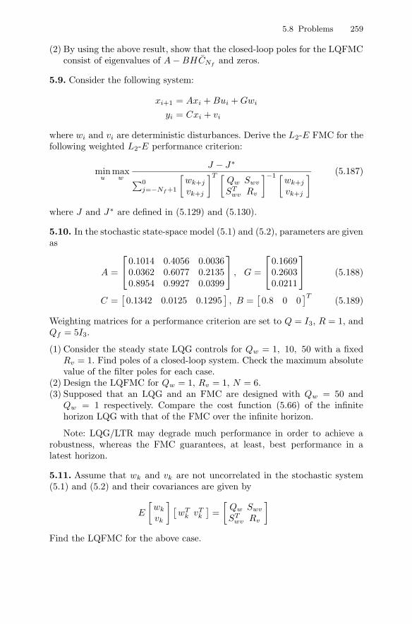
5.8 Problems 259

(2) By using the above result, show that the closed-loop poles for the LQFMCconsist of eigenvalues of A − BHCNf

and zeros.

5.9. Consider the following system:

xi+1 = Axi + Bui + Gwi

yi = Cxi + vi

where wi and vi are deterministic disturbances. Derive the L2-E FMC for thefollowing weighted L2-E performance criterion:

minu

maxw

J − J∗

∑0j=−Nf+1

[wk+j

vk+j

]T [Qw Swv

STwv Rv

]−1 [wk+j

vk+j

] (5.187)

where J and J∗ are defined in (5.129) and (5.130).

5.10. In the stochastic state-space model (5.1) and (5.2), parameters are givenas

A =

⎡⎣0.1014 0.4056 0.00360.0362 0.6077 0.21350.8954 0.9927 0.0399

⎤⎦ , G =

⎡⎣0.16690.26030.0211

⎤⎦ (5.188)

C =[0.1342 0.0125 0.1295

], B =

[0.8 0 0

]T (5.189)

Weighting matrices for a performance criterion are set to Q = I3, R = 1, andQf = 5I3.

(1) Consider the steady state LQG controls for Qw = 1, 10, 50 with a fixedRv = 1. Find poles of a closed-loop system. Check the maximum absolutevalue of the filter poles for each case.

(2) Design the LQFMC for Qw = 1, Rv = 1, N = 6.(3) Supposed that an LQG and an FMC are designed with Qw = 50 and

Qw = 1 respectively. Compare the cost function (5.66) of the infinitehorizon LQG with that of the FMC over the infinite horizon.

Note: LQG/LTR may degrade much performance in order to achieve arobustness, whereas the FMC guarantees, at least, best performance in alatest horizon.

5.11. Assume that wk and vk are not uncorrelated in the stochastic system(5.1) and (5.2) and their covariances are given by

E

[wk

vk

] [wT

k vTk

]=[

Qw Swv

STwv Rv

]Find the LQFMC for the above case.

260 5 Output Feedback Receding Horizon Controls

5.12. Find an optimal FMC for the following performance criterion

minu

maxw

∑Nc

j=0(uk+j − u∗k+j)

T (uk+j − u∗k+j)∑Nc

j=−Nf+1 wTk+jwk+j

(5.190)

where u∗ is an optimal state feedback control.

5.13. Derive the H∞ FMC for the general A if possible.

5.14. Consider the system model (4.246)-(4.247). The system noise covarianceis 0.02 and the measurement noise covariance is 0.02.1) For δk = 0, obtain an LQ FMC with the horizon length N = 10.2) For δk = 0, obtain an LQG controller.3) For δk = 0, perform simulations for the LQ FMC and LQG controller. Andthen compare them.4) Perform simulations on the time interval [0, 250] under the temporary un-certainty

δk =

0.1, 50 ≤ k ≤ 1000, otherwise (5.191)

5.15. Derive the FMC to minimize the following cost function:

2γ2 log E exp[

12γ2

N−1∑i=0

[xTk+iQxk+i + uT

k+iRuk+i] + xTk+NQfxk+N

](5.192)

for a state-space model (5.1) and (5.2) and a fixed γ. Unbiasedness conditions(5.94) and (5.95) are required.

6

Constrained Receding Horizon Controls

6.1 Introduction

In many control systems, input variables cannot be arbitrarily large and mayhave some limitations, such as magnitude limits, since input devices are valves,motors and pumps, etc. Also, state values must be bounded in many cases. Forexample, in process plants, the temperature or the pressure as state variablesmust be within certain limits because of safety. As pointed before, many usefulcontrols can be obtained from optimal controls on the infinite horizon. Thesecontrols for the infinite horizon are difficult to obtain, particularly for inputand state constraints. However, optimal controls for the finite horizon arerelatively easy to obtain for linear systems with input and state constraintsby using SDP. Since receding horizon control is based on the finite horizon,receding horizon controls can handle input and state constraints. Althoughconstrained systems are difficult to stabilize by using conventional controls,RHC provides a systematic way to stabilize the closed-loop system.

Similar to linear systems, the cost monotonicity holds for constrained sys-tems under certain conditions, together with feasibility conditions. Stabilitycan be guaranteed under a cost monotonicity condition. The cost monotonic-ity condition for the constrained RHC can be obtained by three approaches,i.e. the terminal equality constraint, the free terminal cost, and the terminalinvariant set with or without a terminal cost.

It takes a relatively long time to calculate the constrained RHC. Thus, itis necessary to introduce fast algorithms that require less computation time.The feasibility is also an important issue for guaranteeing the existence of theoptimal control satisfying constraints. Output feedback RHCs for constrainedsystems are necessary if the state is not available.

The organization of this chapter is as follows. In Section 6.2, input andoutput constraints, together with reachable and maximal output admissiblesets, are discussed for the feasibility. In Section 6.3, constrained receding hori-zon LQ controls are represented in LMI forms. In Section 6.4, the RHC witha terminal equality and a terminal cost is introduced for constrained systems.

262 6 Constrained Receding Horizon Controls

In particular, a cost monotonicity condition is presented in order to guaranteethe stability. In Section 6.5, constrained RHCs with a terminal invariant setare introduced for constrained systems. Soft constrains are dealt with in Sec-tion 6.6. In Section 6.7, constrained output feedback receding horizon controlsare introduced.

6.2 Reachable and Maximal Output Admissible Sets

In this section we will consider the following linear discrete time-invariantsystem:

xi+1 = Axi + Bui (6.1)

with input and state constraints:−ulim ≤ ui ≤ ulim, i = 0, 1, · · · ,∞−glim ≤ Gxi ≤ glim, i = 0, 1, · · · ,∞ (6.2)

where ulim ∈ m, G ∈ ng×n, and g ∈ ng . It is noted that the inequalityin (6.2) holds component by component. Since Gxi can be considered as anoutput, −glim ≤ Gxi ≤ glim in (6.2) is often called an output constraint. Thesystem (6.1) with constraints (6.2) is said to be feasible if there exist sequencesfor an input and a state that satisfy (6.1) and (6.2). Constraints (6.2) can bewritten as

Euk ≤ e, Gxk ≤ g, k = 0, 1, 2, · · · (6.3)

where

E =[

I−I

], e =

[ulim

−ulim

], G =

[G−G

], g =

[glim

−glim

](6.4)

U and X are defined as

U = u| − ulim ≤ u ≤ ulimX = x| − glim ≤ Gx ≤ glim

In order to observe how the input constraint has an effect on the system, itwill be interesting to investigate all possible states that can be reached fromthe initial state by all available controls. For simplicity, the initial state isconsidered to be the origin. The reachable set is defined as

RN=

x(N ;x0, u)∣∣∣∣x0 = 0, ui ∈ U , 0 ≤ i ≤ N − 1

(6.5)

In order to see whether the state constraint is violated or not, it will beinteresting to investigate all possible initial states, from which all states belong

6.2 Reachable and Maximal Output Admissible Sets 263

to X . For simplicity, the input is considered to be zero. The maximal outputadmissible set O∞ is the largest output admissible set, namely the set of allinitial states x0, which makes the resultant state trajectory xi satisfy xi ∈ Xfor all i > 0.

O∞= x0 | x(i;x0) ∈ X , ∀i = 0, 1, 2., · · · (6.6)

Reachable Sets

Consider the linear system

xk+1 = Axk + Buk (6.7)

where A ∈ n, B ∈ m, n ≥ m, and B is of full rank.Let RN denote the set of reachable states with unit total input energy

RN=

xN

∣∣∣∣x0 = 0,N−1∑i=0

uTi ui ≤ 1

(6.8)

Constraints on total input energy often appear in optimization problems.Suppose that there exists a Lyapunov function Vk = xT

k Pxk such that

Vk+1 − Vk ≤ uTk uk (6.9)

for every xk and uk. Then, summing up from k = 0 to k = N − 1 yields

VN − V0 ≤N−1∑k=0

uTk uk (6.10)

Noting that V0 = xT0 Px0 = 0 since x0 = 0, we get

VN ≤N−1∑k=0

uTk uk ≤ 1 (6.11)

for every input uk satisfying the constraint in (6.8). Thus, the set xN |xTNPxN

≤ 1 contains the reachable set RN . It follows from (6.9) that we have

Vk+1 − Vk = (Axk + Buk)T P (Axk + Buk) − xTk Pxk ≤ uT

k uk (6.12)

leading to [xk

uk

]T [AT PA − P AT PB

BT PA BT PB − I

] [xk

uk

]≤ 0 (6.13)

From the above equation, P can be obtained by[AT PA − P AT PB

BT PA BT PB − I

]≤ 0 (6.14)

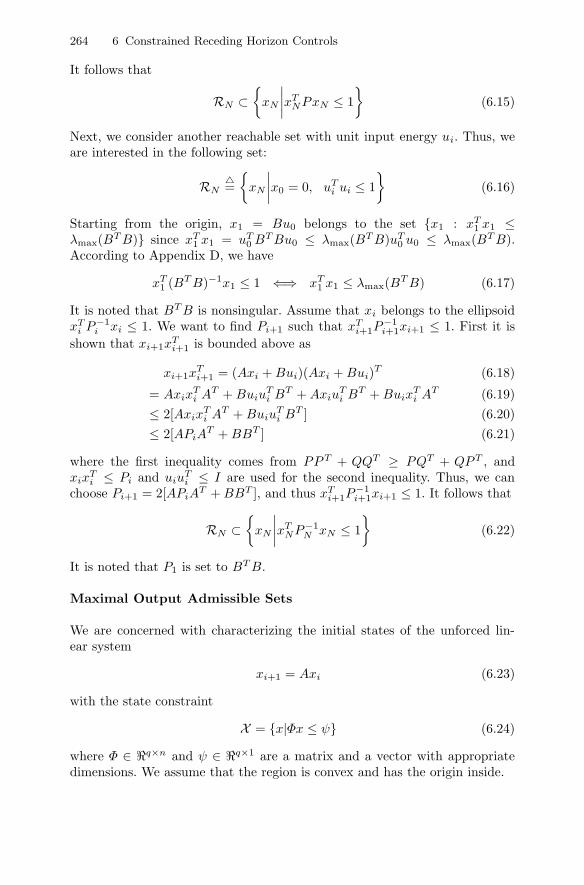
264 6 Constrained Receding Horizon Controls

It follows that

RN ⊂

xN

∣∣∣∣xTNPxN ≤ 1

(6.15)

Next, we consider another reachable set with unit input energy ui. Thus, weare interested in the following set:

RN=

xN

∣∣∣∣x0 = 0, uTi ui ≤ 1

(6.16)

Starting from the origin, x1 = Bu0 belongs to the set x1 : xT1 x1 ≤

λmax(BT B) since xT1 x1 = uT

0 BT Bu0 ≤ λmax(BT B)uT0 u0 ≤ λmax(BT B).

According to Appendix D, we have

xT1 (BT B)−1x1 ≤ 1 ⇐⇒ xT

1 x1 ≤ λmax(BT B) (6.17)

It is noted that BT B is nonsingular. Assume that xi belongs to the ellipsoidxT

i P−1i xi ≤ 1. We want to find Pi+1 such that xT

i+1P−1i+1xi+1 ≤ 1. First it is

shown that xi+1xTi+1 is bounded above as

xi+1xTi+1 = (Axi + Bui)(Axi + Bui)T (6.18)

= AxixTi AT + Buiu

Ti BT + Axiu

Ti BT + Buix

Ti AT (6.19)

≤ 2[AxixTi AT + Buiu

Ti BT ] (6.20)

≤ 2[APiAT + BBT ] (6.21)

where the first inequality comes from PP T + QQT ≥ PQT + QPT , andxix

Ti ≤ Pi and uiu

Ti ≤ I are used for the second inequality. Thus, we can

choose Pi+1 = 2[APiAT + BBT ], and thus xT

i+1P−1i+1xi+1 ≤ 1. It follows that

RN ⊂

xN

∣∣∣∣xTNP−1

N xN ≤ 1

(6.22)

It is noted that P1 is set to BT B.

Maximal Output Admissible Sets

We are concerned with characterizing the initial states of the unforced lin-ear system

xi+1 = Axi (6.23)

with the state constraint

X = x|Φx ≤ ψ (6.24)

where Φ ∈ q×n and ψ ∈ q×1 are a matrix and a vector with appropriatedimensions. We assume that the region is convex and has the origin inside.

6.2 Reachable and Maximal Output Admissible Sets 265

A set O is output admissible if x0 ∈ O implies that xi ∈ X for all k >0. The maximal output admissible set O∞ is the largest output admissibleset, namely the set of all initial states x0, which makes the resultant statetrajectory xi remain inside forever, i.e. xi ∈ X for all i > 0. This set isvisualized in Figure 6.1. A set X is invariant if x0 ∈ X implies that xi ∈ Xfor all i > 0. It is noted that the maximal output admissible set is alwaysinvariant.

Fig. 6.1. Graphical representation of the maximal output admissible set

The maximal output admissible set is defined as

O∞(A,Φ, ψ) = x|ΦAkx ≤ ψ, ∀k = 0, 1, 2., · · · (6.25)

Define the set Oi as

Oi(A,Φ, ψ) = x|ΦAkx ≤ ψ, ∀k = 0, 1, 2., · · · , i (6.26)

Obviously, the set Oi(A,Φ, ψ) satisfies the condition

O∞ ⊂ Oi2 ⊂ Oi1 (6.27)

for all i1 and i2 such that i1 ≤ i2. Now, it may happen that the sequence ofsets Oi (i = 1, 2, · · · ) stops getting smaller as i increases. That is, there maybe the smallest value of i∗ such that Oi = Oi∗ for all i ≥ i∗. We call i∗ theoutput admissibility index. In that case, it is clear that O∞ = Oi∗ .

We say O∞ is finitely determined if, for some i, O∞ = Oi. O∞ is finitelydetermined if and only if Oi = Oi+1 for some i.

If (A,Φ) is observable, then it is known that O∞ is convex and bounded.Additionally, O∞ contains an origin in its interior if A is stable. It is alsoknown that if A is a stable matrix, (A,Φ) is observable, X is bounded, and Xcontains zero, then O∞ is finitely determined.

If O∞ is finitely determined, then the algorithm will terminate for somevalue i = i∗ and

O∞ = x|ΦAix ≤ ψ, 0 ≤ i ≤ i∗ (6.28)

266 6 Constrained Receding Horizon Controls

The following algorithm describes how to obtain O∞. Basically, this algo-rithm is based on linear programming, so it can be solved efficiently.

Algorithm for obtaining maximal output admissible set

1. Take j = 0.2. For i = 1 to q, solve the following linear programming problem:

Ji = maxz

ΦiAj+1z subject to ΦAkz ≤ ψ,∀k = 0, 1, · · · , j

where Φi denotes the ith row of the matrix Φ.3. If Ji > ψi for i = 1 to q, take j = j + 1 and repeat the previous

step.4. If Ji ≤ ψi for i = 1 to q, then O∞ = Oj .

Example 6.1

The unforced linear system and state constraints are given as

xi+1 =[

0.9746 0.1958−0.1953 0.5839

]xi

Φ =

⎡⎢⎢⎢⎢⎢⎢⎣−0.8831 −0.88110.8831 0.88111.0000 0−1.0000 0

0 1.00000 −1.0000

⎤⎥⎥⎥⎥⎥⎥⎦ ψ =

⎡⎢⎢⎢⎢⎢⎢⎣0.50000.50001.50001.50000.30000.3000

⎤⎥⎥⎥⎥⎥⎥⎦Figure 6.2 shows the region corresponding to the O∞ for the above system.

Maximal Output Admissible Set for Constrained Infinite HorizonLinear Quadratic Regulator

The cost function to be minimized is given by

J∞ =∞∑

k=0

[xT

k Qxk + uTk Ruk

](6.29)

subject to (6.3).It is well known that the steady-state LQR for an unconstrained system

is given by

uk = Kxk (6.30)

for some K. The input constraint is equivalently changed into the state con-straint as follows:

6.2 Reachable and Maximal Output Admissible Sets 267

−0.8 −0.6 −0.4 −0.2 0 0.2 0.4 0.6 0.8−0.4

−0.3

−0.2

−0.1

0

0.1

0.2

0.3

x1

x 2

Fig. 6.2. Maximal output admissible sets

Euk ≤ e ⇐⇒ EKxk ≤ e (6.31)

Then the total constraint is given by

Φx ≤ ψ (6.32)

where

Φ =[

EKG

]ψ =

[eg

](6.33)

The closed-loop system is represented by

xk+1 = Aclxk (6.34)yk = Cxk (6.35)

where Acl = A + BK. Because the control uk = Kxk is optimal in the casethat the system is unconstrained, it may not be optimal for the actual system,which has input and state constraints. However, if the initial state x0 is in acertain region, then the input and the state constraints will never be activeand thus the control uk = Kxk for an unconstrained optimal problem isoptimal for a constrained optimal problem. We will obtain such a region forx0. We can conclude that if x0 belongs to O∞(Acl, Φ, ψ), then (6.30) becomesoptimal for the performance criterion (6.29) with constraints (6.32).

If x0 does not belong to O∞(Acl, Φ, ψ), then we will use another controlscheme. An optimal control is used for the finite horizon from the initial timein order to make the final state xN on the horizon enter O∞(Acl, Φ, ψ), andthe steady-state optimal control uk = Kxk is used for the remaining infinitehorizon.

268 6 Constrained Receding Horizon Controls

Note that the J∞ can be decomposed as

J∞ =N−1∑k=0

[xT

k Qxk + uTk Ruk

]+

∞∑k=N

[xT

k Qxk + uTk Ruk

](6.36)

If xN ∈ O∞(Acl, Φ, φ), then the cost function on [N, ∞] can be representedas

∞∑k=N

[xT

k Qxk + uTk Ruk

]= xT

NPxN (6.37)

where P is obtained from the following steady-state Riccati equation:

P = AT PA − AT PB[R + BT PB]−1BT PA + Q (6.38)

Therefore, in a certain the case, the cost J∞ can be rewritten as

JN =N−1∑k=0

[xT

k Qxk + uTk Ruk

]+xT

NPxN (6.39)

Observe that the original infinite horizon cost J∞ can be equivalently replacedby a finite horizon cost JN .

Consider the following optimization problem with constraints:

minui

JN (6.40)

subject to

Euk ≤ e,Gxk ≤ g, k = 0, 1, · · · , N − 1 (6.41)

Assume that the problem is feasible. Let us denote the optimal control andthe resultant state by u∗

k and x∗k respectively. We will use the control strategy

uk = u∗k, k = 0, 1, · · · , N − 1

uk = Kxk, k = N,N + 1, · · ·(6.42)

It is clear that uk and xk, k = 0, 1, · · · , N − 1, satisfy the given inputand the state constraints. However, it is not guaranteed that uk and xk

for k = N,N + 1, · · · satisfy the given constraints. We can conclude thatif xN ∈ O∞(Acl, Φ, φ), uk and xk for k = N,N + 1, · · · satisfy the given con-straints.

6.3 Constrained Receding Horizon Control with Terminal Equality Constraint 269

6.3 Constrained Receding Horizon Control withTerminal Equality Constraint

Input and State Constraints

The system (6.1) and the constraints (6.2) can be represented in the pre-dictive form

xk+j+1 = Axk+j + Buk+j (6.43)

with input and state constraints:−ulim ≤ uk+j ≤ ulim, j = 0, 1, · · · , N − 1−glim ≤ Gxk+j ≤ glim, j = 0, 1, · · · , N

(6.44)

States on [k, k + N ] can be represented as

Xk = Fxk + HUk (6.45)

where Xk, F , H and Uk are given by

Uk =

⎡⎢⎢⎢⎣uk

uk+1

...uk+N−1

⎤⎥⎥⎥⎦ , Xk =

⎡⎢⎢⎢⎣xk

xk+1

...xk+N−1

⎤⎥⎥⎥⎦ , F =

⎡⎢⎢⎢⎣IA...

AN−1

⎤⎥⎥⎥⎦ (6.46)

H =

⎡⎢⎢⎢⎢⎢⎣0 0 0 · · · 0B 0 0 · · · 0

AB B 0 · · · 0...

.... . .

......

AN−2B AN−3B · · · B 0

⎤⎥⎥⎥⎥⎥⎦ (6.47)

Each state on the horizon [k, k + N ] is given by

xk+j = Ajxk + BjUk (6.48)

where

Bj=[Aj−1B Aj−2B · · · B O · · · O

](6.49)

Constraints (6.44) can be written as⎡⎢⎢⎢⎣−ulim

−ulim

...−ulim

⎤⎥⎥⎥⎦ ≤ Uk ≤

⎡⎢⎢⎢⎣ulim

ulim

...ulim

⎤⎥⎥⎥⎦ (6.50)

⎡⎢⎢⎢⎣−glim

−glim

...−glim

⎤⎥⎥⎥⎦ ≤ GN (Fxk + HUk) ≤

⎡⎢⎢⎢⎣glim

glim

...glim

⎤⎥⎥⎥⎦ (6.51)

270 6 Constrained Receding Horizon Controls

whereGN = diagG, · · · , G︸ ︷︷ ︸

N

Input and state constraints in (6.50) and (6.51) can be converted to LMI formas follows:

em×j+lUk − ullim ≤ 0,

−em×j+lUk − ullim ≤ 0, l = 1, 2, · · · ,m, j = 0, 1, · · · , N − 1 (6.52)

eTng×j+qGN (Fxk + HUk) − gq

lim ≤ 0−eT

ng×j+qGN (Fxk + HUk) − gqlim ≤ 0 j = 0, 1, · · · , N, q = 1, 2, · · · , ng (6.53)

where es is a vector such that es = [0, · · · , 0, 1, 0, · · · , 0]T with the nonzeroelement in the sth position, and xa implies the ath component of the vectorx. The inequality (6.53) can be also written as

eq(G(Ajxk + BjUk)) − gqlim ≤ 0

−eq(G(Ajxk + BjUk)) − gqlim ≤ 0 (6.54)

Solution in Linear Matrix Inequality Form

Here, we consider the following performance criterion and the terminal equal-ity constraint:

J(xk, k) =N−1∑j=0

(xTk+jQxk+j + uT

k+jRuk+j) (6.55)

xk+N = 0 (6.56)

where Q ≥ 0 and R > 0. If there is a feasible solution for the system (6.43)and the performance criterion (6.55) with constraints (6.56) at the initial timek0, then the next solution is guaranteed to exist, since at least one feasiblesolution u[k+1,k+N ] = [u[k+1,k+N−1] 0] exists.

For (6.56), it is required to satisfy

ANxk + BUk = 0 (6.57)

where B = BN is given by[AN−1B AN−2B · · · B

](6.58)

and Uk is defined in (6.47). We parameterize Uk in (6.57) in terms of knownvariables. If we use the following correspondences in Lemma A.3:

A → B

X → Uk

Y → − ANxk

6.3 Constrained Receding Horizon Control with Terminal Equality Constraint 271

then it can be seen that all solutions Uk to (6.57) are parameterized by

Uk = −B−1ANxk + MUk (6.59)

where Uk is a matrix containing the independent variables, B−1 is the rightinverse of B, and columns of M are orthogonal to each other, spanning thenull space of B. It is noted that B−1 = BT (BBT )−1. The control (6.59)can be combined with the receding horizon control with the terminal equalityconstraint in Section 3.5.2.

The optimization problem for the fixed terminal case is reduced to thefollowing SDP:

min γ1 (6.60)[γ1 − V3 − V2Uk −UT

k V121

−V121 Uk I

]≥ 0

subject to(6.52) and (6.53)

where

V1 = MT WM

V2 = −2(ANxk − xrk+N )T B−T WM + wT M

V3 = (ANxk − xrk+N )T B−T WB−1(ANxk − xr

k+N )

+ [Fxk − Xrk ]T QN [Fxk − Xr

k ] − wT B−1(ANxk − xrk+N )

W = HT QNH + RN

w = 2xTk FT QNH

and QN and RN are defined in (3.312).It is noted that Uk is obtained from the SDP problem (6.60) and Uk is

computed from Uk according to (6.59).

Theorem 6.1. The optimization problem based on (6.43), (6.44), (6.55), and(6.56) can be formulated into an SDP (6.60).

What remains to do is just to pick the first one up among U ∗k as

u∗k =

[1, 0, · · · , 0

]U∗

k (6.61)

Cost Monotonicity

We already learned in Chapter 3 that the equality condition xk+N = 0 pro-vides the cost monotonicity condition, which also holds in constrained systemsaccording to the following theorem.

272 6 Constrained Receding Horizon Controls

Theorem 6.2. Assume that the system is feasible on [k, σ] with the terminalequality constraint. Then the optimal cost J∗(xτ , τ, σ) for the terminal equalityconstraint satisfies the following monotonicity relation:

J∗(xτ , τ, σ + 1) ≤ J∗(xτ , τ, σ), τ ≤ σ (6.62)

Proof. The proof procedure is the same as Theorem 3.1, except that thereexist the inputs and the corresponding states that satisfy the constraints.This completes the proof.

Stability

We have the following result on the stability of the constrained RHCs.

Theorem 6.3. Assume that the system is feasible at the initial time and somehorizon N∗ with the terminal equality constraint and Q is positive definite.The receding horizon LQ control with the terminal equality constraint stabilizesthe closed-loop system (6.1) for all horizons N ≥ N ∗.

Proof. The proof procedure is the same as Theorem 3.7, except that there existinputs and corresponding states that satisfy the constraints. This completesthe proof.

6.4 Constrained Receding Horizon Control withTerminal Set Constraint

In a fixed terminal case, the condition xk+N = 0 is too strong to have asolution satisfying all constraints. Thus, we relax this condition and requirethat the terminal state has only to enter some ellipsoid instead of going intothe origin exactly, which is depicted in Figure 6.3.

Using the property of the invariant ellipsoid, we introduce a receding hori-zon dual-mode control that satisfies the constraints on the input and the state.Outside the ellipsoid, the receding horizon control is employed. Once the stateenters the ellipsoid, the control is switched to a linear state feedback control,which makes the state stay in the ellipsoid forever and stabilizes the system.This is called a receding horizon dual-mode control.

Terminal Invariant Set for ui = Hxi

Now, we will try to find a stable linear feedback control that meets all in-put and state constraints within the terminal ellipsoid (6.78) and make thestate stay inside forever.

We define an ellipsoid EQf ,α centered at the origin:

6.4 Constrained Receding Horizon Control with Terminal Set Constraint 273

Generalization

Constraints

Fig. 6.3. Terminal ellipsoid constraint and terminal equality constraint

EQf ,α = x ∈ Rn|xT Qfx < α (6.63)

We will choose a stable linear feedback control ui = Hxi so that it meets allgiven input and state constraints

−ulim ≤ ui ≤ ulim (6.64)−glim ≤ Gxi ≤ glim (6.65)

within the ellipsoid (6.78) and make the state stay inside forever.The condition

(A − BH)T Qf (A − BH) − Qf < 0 (6.66)

leads to

‖xi+1‖2Qf

− ‖xi‖2Qf

= xTi [(A − BH)T Qf (A − BH) − Qf ]xi < 0 (6.67)

The matrix inequality (6.66) is converted to the LMI as[Qf A − BH

(A − BH)T Q−1f

]< 0[

X AX − BYXAT − Y T BT X

]< 0 (6.68)

where X = Q−1f and Y = HX.

Therefore, the state trajectory xi, i > 0, with the state feedback controlui = Hxi remains in the ellipsoid EQf ,α and approaches zero asymptotically.

Now we will investigate if the input constraint (6.64) is satisfied in theregion EQf ,α. First, we consider the jth element of ui at time step i whichsatisfies the constraint

|uji | ≤ uj

lim, j ≥ 0, j = 1, · · · ,m (6.69)

274 6 Constrained Receding Horizon Controls

where ujlim is the jth element of ulim.

Recall that (xT x) ≥ (lT x)2 for any vectors x and l with lT l = 1. Then,

maxi≥0

|uji |2 = max

i≥0,xi∈EQf

|(Y X−1xi)j |2

≤ maxz∈EQf ,α

|(Y X−1z)j |2 = maxz∈EQf ,α

|(Y X− 12 X− 1

2 z)j |2

= maxwT w≤α

|(Y X− 12 w)j |2 = α|EjY X− 1

2 |22 = αEjY X−1Y T ETj (6.70)

where Ej is the jth unit row vector with the nonzero element in the jthposition

Ej=[0 · · · 0 1 0 · · · 0

]Note that Ej plays a role in selecting the jth row of a matrix by pre-multiplication.

From (6.69) and (6.70), we have αEjY X−1Y T ETj ≤ uj

lim, which can beconverted to the following LMI:[

(ujlim)2 EjY

(EjY )T 1αX

]> 0 (6.71)

for j = 1, 2, · · · ,m.The state constraint (6.65) can be checked with a similar procedure.

maxi≥0

|(Gxi)j |2 ≤ maxz∈EQf

|(GX12 X− 1

2 z)j |2 = max|w|22=α

|(GX12 w)j |2

= α|EjGX12 |22 = αEjGXGT ET

j (6.72)

From (6.72), the LMI for the state constraint is obtained:

[(gj

lim)2 EjGXXT (EjG)T α−1X

]> 0 (6.73)

For constrained systems, we should make the ellipsoid shrink so that thestate feedback control ui = Hxi asymptotically stabilizes the system whilesatisfying the input and the state constraints. Based on this fact, we introducethe following lemma.

Lemma 6.4. Suppose that there exist X > 0 and Y satisfying the LMIs(6.68), (6.71), and (6.73). For the state feedback controller ui = Y X−1xi =Hxi, the resultant state trajectory xi always remains in the region EQf ,α sat-isfying the constraints on the input and the state.

According to Lemma 6.4, the input and state constraints are expressedby each component. This may be rewritten in another form to consider theconstraints in terms of one LMI.

6.4 Constrained Receding Horizon Control with Terminal Set Constraint 275

If we introduce another variable Z that satisfies

αEjY X−1Y T ETj = α(Y X−1Y T )j,j ≤ Zj,j ≤ uj

lim

where Zj,j is (j, j) elements of the matrices Z, αY X−1Y T ≤ Z implies thatthe input constraint −ulim ≤ ui ≤ ulim is guaranteed in the region EX .Therefore, we obtain the following LMI:[

Z YY T 1

αX

]≥ 0, with Zj,j ≤ (uj

lim)2 (6.74)

If we introduce a variable V that satisfies

α(GXGT )j,j ≤ Vj,j ≤ gjlim

then αGXGT ≤ V implies that the state constraint −glim ≤ Gxi ≤ glim isguaranteed in the region EQf ,α. Therefore, we obtain the following LMI:

αGXGT ≤ V, with Vj,j ≤ (gjlim)2 (6.75)

In order for a dual-mode control to stabilize the system, the state must enterthe ellipsoid within the given finite time

Constrained Receding Horizon Dual-mode Control with Fixed In-variant Set

The following performance is considered:

J1(xk, k)=

Nk−1∑j=0

(xTk+jQxk+j + uT

k+jRuk+j) (6.76)

with the input and state constraints−ulim ≤ uk+j ≤ ulim, j = 0, 1, · · · , Nk − 1−glim ≤ Gxk+j ≤ glim, j = 0, 1, · · · , Nk

(6.77)

and the terminal set constraint

xTk+NPxk+N ≤ α (6.78)

which is represented as

EP,α = x ∈ Rn|xT Px ≤ α (6.79)

The terminal set (6.78) can be written as

(ANkxk + BUk)T P (ANkxk + BUk) < α

276 6 Constrained Receding Horizon Controls

which is converted into the following LMI:[α (ANkxk + BUk)T

(ANkxk + BUk) P−1

]> 0 (6.80)

According to (3.319) and (3.320) in Section 3.5.2, the problem minimizing(6.76) is reduced to the following LMI form:[

γ1 − wT Uk − xTk FT

k QNFkxk UTk

Uk W−1

]≥ 0 (6.81)

We try to find the minimum γ1 subject to (6.81), (6.52), (6.53), and (6.80) toobtain an optimal control which steers the state into the ellipsoid (6.79).

Dual-mode control can be obtained as follows: at time k = 0, if x0 ∈E , switch to a local linear control, i.e. employ a linear feedback law uk =Kxk thereafter such that xk ∈ E . Otherwise, compute a control horizon pair(u0+·, N0) for the problem J(x0, 0, u0+·, N0). Apply the control u0 to the realsystem.

Assume that the control pair (uk−1+·, Nk−1) is found. At the time k, if xk ∈E , switch to a local linear control, i.e. employ the linear feedback control lawKxk thereafter such that xk ∈ E . Otherwise, we compute another admissiblecontrol horizon pair (uk+·, Nk), which is better than the preceding controlhorizon pair in the sense that

J(xk, k, uk+·, Nk) ≤ J(xk, k, u′k+·, Nk−1 − 1) (6.82)

where u′k+· is equal to uk−1+· in the interval [k, k − 1 + Nk−1] and is an

admissible control for J(xk, k, uk+·, Nk). Finally, we apply the control uk tothe real system.

The control uk always exists, since there is at least one feasible solution ifNk is set to Nk−1 − 1. It is noted that Nk is time-varying, whereas N is fixedin previous sections.

Theorem 6.5. Suppose that the system (6.1) is stabilizable. Then, for Nk >1, there exists a control horizon pair (uk, Nk) such that the following equationis satisfied:

J(xk, k, uk, Nk) ≤ J(xk, k, u′k, Nk−1 − 1) (6.83)

and there exists constant 0 < η < ∞ satisfying

J(xk+1, k + 1, uk+1, Nk+1) ≤ J(xk, k, uk, Nk) − η (6.84)

for all k such that both xk and xk+1 are in EP,α.

Proof. The first statement is already explained in (6.82). Since the trajectoryby (uk, Nk) is the same as one by (uk+1, Nk − 1) on [k + 1, k + Nk], we have

6.5 Constrained Receding Horizon Control with Free Terminal Cost 277

J(xk, k, uk, Nk) − J(xk+1, k + 1, u′k+1, Nk − 1) (6.85)

= xTk Qxk + uT

k Ruk (6.86)≥ infxT

k Qxk | xk ∈ EP,α (6.87)

= infxT Qx

xT PxxT Px | x ∈ EP,α (6.88)

≥ λmin(Q)λmax(P )

α (6.89)

for all k such that both xk and xk+1 lie in EP,α. Thus, η can be taken as

η =λmin(Q)λmax(P )

α (6.90)

This completes the proof.

Theorem 6.6. The dual-mode receding horizon controller is asymptoticallystabilizing with a region of attraction X. For all x0 ∈ X, there exists a finitetime N∗ such that xN∗ ∈ EP,α.

Proof. Suppose that there is no such k for which xk ∈ EP,α. From Theorem6.5, it follows that there exists a 0 < η < ∞ such that

J(xk+1, k + 1, uk+1+·, Nk+1) ≤ J(xk, k, uk+·, Nk) − η (6.91)

for all k, which immediately implies that

J(xk, k, uk+·, Nk) < 0 (6.92)

for some k > 0. However, this contradicts the fact that

J(xk, k, uk+·, Nk) ≥ 0 (6.93)

for all k. Therefore, there exists a finite k such that xk ∈ EP,α. xk enters EP,α

within a finite time and then approaches zero by a local linear stabilizing statefeedback control. This completes the proof.

The horizon N is varying with time in the above cases. However, we canuse the fixed horizon N with a stability property. We introduce a dual-modecontrol with a stability property, which will be explained later.

6.5 Constrained Receding Horizon Control with FreeTerminal Cost

Solution in Linear Matrix Inequality Form

The performance criterion can be written into two parts as follows:

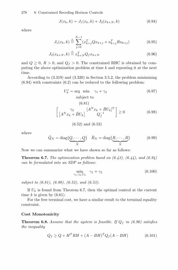
278 6 Constrained Receding Horizon Controls

J(xk, k) = J1(xk, k) + J2(xk+N , k) (6.94)

where

J1(xk, k)=

N−1∑j=0

(xTk+jQxk+j + uT

k+jRuk+j) (6.95)

J2(xk+N , k)= xT

k+NQfxk+N (6.96)

and Q ≥ 0, R > 0, and Qf > 0. The constrained RHC is obtained by com-puting the above optimization problem at time k and repeating it at the nexttime.

According to (3.319) and (3.320) in Section 3.5.2, the problem minimizing(6.94) with constraints (6.2) can be reduced to the following problem:

U∗k = arg min γ1 + γ2 (6.97)

subject to(6.81)[

γ2 [ANxk + BUk]T[ANxk + BUk

]Q−1

f

]≥ 0 (6.98)

(6.52) and (6.53)

whereQN = diagQ, · · · , Q︸ ︷︷ ︸

N

RN = diagR, · · · , R︸ ︷︷ ︸N

(6.99)

Now we can summarize what we have shown so far as follows:

Theorem 6.7. The optimization problem based on (6.43), (6.44), and (6.94)can be formulated into an SDP as follows:

minγ1,γ2,Uk

γ1 + γ2 (6.100)

subject to (6.81), (6.98), (6.52), and (6.53).

If Uk is found from Theorem 6.7, then the optimal control at the currenttime k is given by (6.61).

For the free terminal cost, we have a similar result to the terminal equalityconstraint.

Cost Monotonicity

Theorem 6.8. Assume that the system is feasible. If Qf in (6.96) satisfiesthe inequality

Qf ≥ Q + HT RH + (A − BH)T Qf (A − BH) (6.101)

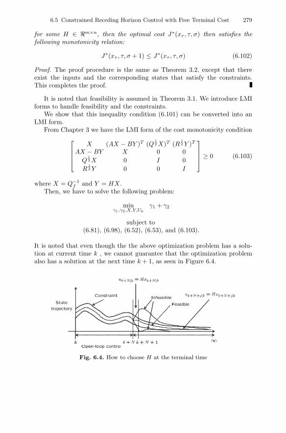
6.5 Constrained Receding Horizon Control with Free Terminal Cost 279

for some H ∈ m×n, then the optimal cost J∗(xτ , τ, σ) then satisfies thefollowing monotonicity relation:

J∗(xτ , τ, σ + 1) ≤ J∗(xτ , τ, σ) (6.102)

Proof. The proof procedure is the same as Theorem 3.2, except that thereexist the inputs and the corresponding states that satisfy the constraints.This completes the proof.

It is noted that feasibility is assumed in Theorem 3.1. We introduce LMIforms to handle feasibility and the constraints.

We show that this inequality condition (6.101) can be converted into anLMI form.

From Chapter 3 we have the LMI form of the cost monotonicity condition⎡⎢⎢⎣X (AX − BY )T (Q

12 X)T (R

12 Y )T

AX − BY X 0 0Q

12 X 0 I 0

R12 Y 0 0 I

⎤⎥⎥⎦ ≥ 0 (6.103)

where X = Q−1f and Y = HX.

Then, we have to solve the following problem:

minγ1,γ2,X,Y,Uk

γ1 + γ2

subject to(6.81), (6.98), (6.52), (6.53), and (6.103).

It is noted that even though the the above optimization problem has a solu-tion at current time k , we cannot guarantee that the optimization problemalso has a solution at the next time k + 1, as seen in Figure 6.4.

Fig. 6.4. How to choose H at the terminal time

280 6 Constrained Receding Horizon Controls

Stability

We have the following results on the stability of the constrained RHCs.

Theorem 6.9. Assume that the system is feasible for all k and some N ∗, andQ is positive definite. The receding horizon LQ control with the free terminalcost under a cost monotonicity condition (6.102) stabilizes the closed-loopsystem (6.1) for N ≥ N∗.

Proof. The proof procedure is the same as Theorem 3.8, except that thereexist the inputs and the corresponding states that satisfy the constraints.Since Q > 0, xT

i Qxi → 0 implies xi → 0. This completes the proof.

A feedback control uσ = Hxσ was obtained from Theorem 6.8. We canutilize the state feedback control every time.

Let σ = k; we must have

(A + BH)xk ∈ X , Hxk ∈ U (6.104)

and

−glim ≤ G(A − BH)xk ≤ glim (6.105)−ulim ≤ Hxk ≤ ulim (6.106)

It is noted that H used in uk = Hxk is obtained at the terminal time k.

Theorem 6.10. If the system is feasible and Qf is positive definite, then thestate feedback control ui = Hxi obtained from (6.103), (6.105) and (6.106)stabilizes the closed-loop system while satisfying the constraints.

Proof. Let V (xi) = xTi Qfxi. Since Qf > 0, V (xi) can be a Lyapunov function.

V (xi+1) − V (xi) = xTi (A − BH)T Qf (A − BH)xi − xiQfxi

= xi(−Qf − HT RH)xi

≤ −xTi Qfxi

Thus, xi → 0. This completes the proof.

It is noted that controls in Theorems 6.3, 6.9, and 6.10 are assumed to existat each time. In order to guarantee the feasibility on the infinite horizon, weintroduce an ellipsoid invariant set in the next section.

When certain constraints are imposed on the given system, it is an impor-tant issue whether the optimization problem formulated has a solution for alltimes k.

6.5 Constrained Receding Horizon Control with Free Terminal Cost 281

Terminal Invariant Ellipsoid

From the optimization problem (6.97), we require additional constraint

γ2 ≤ α (6.107)

in order to improve the feasibility.Here, we introduce an algorithm to solve the optimization problem (6.97).

Now, we will use γ∗2 instead of α, which brings out the advantage that it is not

necessary to make the final state driven to the specific ellipsoid. We can obtainthe ellipsoid while optimizing the given performance criterion. The optimalcost xT Qfx for the final state is equal to γ∗

2 , so that we choose Qf and γ∗2

to make the ellipsoid xT Qfx ≤ γ∗2 invariant. For these Qf and γ∗

2 , the finalstate is on the boundary of the ellipsoid xT Qfx ≤ γ∗

2 . Thus, we have only toreplace X with γ2Q

−1f and find it so that the ellipsoid is invariant. The LMIs

(6.71) and (6.73) should be changed to[(uj

lim)2 EjY(EjY )T 1

γ2X

]> 0 (6.108)

and [(gj

lim)2 EjGXXT (EjG)T γ2X

]> 0 (6.109)

Lemma 6.11. Suppose that there exist X > 0 and Y satisfying (6.103),(6.71), and (6.73). Then, the state feedback controller ui = Y X−1xi = Hxi

exponentially stabilizes the closed-loop system for all x0 ∈ EQf ,α while satisfy-ing the constraint (6.2). And the resultant state trajectory xi always remainsin the region EQf ,α.

The following theorem summarizes the stabilizing receding horizon control.

Theorem 6.12. Consider the optimization problem at time k as follows:

minΛ

γ1 + γ2 (6.110)

subject to (6.52), (6.53), (6.81),[γ2I (ANxk + BUk)T

ANxk + BUk X

]≥ 0 (6.111)

⎡⎢⎢⎣X (AX − BY )T (Q

12 X)T (R

12 Y )T

AX − BY X 0 0Q

12 X 0 γ2I 0

R12 Y 0 0 γ2I

⎤⎥⎥⎦ ≥ 0 (6.112)

282 6 Constrained Receding Horizon Controls[(uj

lim)2 Ej Y

Ej YT X

]> 0 (6.113)

[(gj

lim)2 EjGX

XEjGT X

]> 0 (6.114)

where j = 1, 2, · · · ,m, Λ = γ1, γ2, X, Y , Ut. Then, we can obtain Qf = γ2X

and H = Y X−1. If this optimization problem has a solution at the initialtime, then we can obtain a stabilizing receding horizon control for all the timethat satisfies the constraints on the input and the state.

Proof. In order to combine two variables γ2 and X, we introduce X = γ2X.From (6.98), we have[

γ2I (ANxk + BUk)T

ANxk + BUk X

]≥ 0 (6.115)

Representing X in terms of X and scaling elements in the matrix on the leftside of (6.111) yields

T

[γ2I (ANxk + BUk)T

ANxk + BUk γ−12 X

]TT (6.116)

=[

I (ANxk + BUk)T

ANxk + BUk X

]≥ 0 (6.117)

where

T =[√

γ2−1 0

0√

γ2

](6.118)

Thus, we obtain the LMI (6.111). By using X instead of X, the left side ofthe LMI (6.103) for the cost monotonicity condition can be changed into⎡⎢⎢⎣

γ−12 X γ−1

2 (AX − BY )T (Q12 γ−1

2 X)T (R12 γ−1

2 Y )T

γ−12 (AX − BY ) γ−1

2 X 0 0Q

12 γ−1

2 X 0 I 0R

12 γ−1

2 Y 0 0 I

⎤⎥⎥⎦ (6.119)

Multiplying (6.119) by T2 given as

T2 = diag√γ2,√

γ2,√

γ2,√

γ2

yields (6.112). The input and the state constraints (6.108) and (6.109) in anellipsoid can be represented in a form of the LMIs as[

I 00 γ2I

] [(uj

lim)2 EjYEjY

T 1γ2

X

] [I 00 γ2I

]=[

(ujlim)2 Ej Y

Ej YT X

]> 0 (6.120)

6.5 Constrained Receding Horizon Control with Free Terminal Cost 283

and [I 00 γ2I

] [(gj

lim)2 EjGXXEjG

T γ−12 X

] [I 00 γ2I

]=[

(gjlim)2 EjGX

XEjGT X

]> 0 (6.121)

This completes the proof.

The trajectory of the receding horizon control of Theorem 6.12 is depictedin Figure 6.5.

Fig. 6.5. State trajectory due to the proposed RHC in Theorem 6.12

Example 6.2

To illustrate the validity of the RHC, numerical examples are given for alinear discrete time-invariant system

xi+1 =[

1 0.22120 0.7788

]xi +

[0.02880.2212

]ui (6.122)

where the initial state is set to [1 0.3]T , and ui and xi should be constrainedin the following region:

−0.5 ≤ ui ≤ 0.5 (6.123)[−1.5−0.3

]≤ Gxi =

[1 0 1.50 1 1

]xi ≤

[1.50.3

](6.124)

Here, the performance criterion is taken as4∑

j=0

[ xTk+jxk+j + u2

k+j ] + xTk+5Qfxk+5 (6.125)

where Qf is determined each time. State trajectories are shown in Figure 6.6.

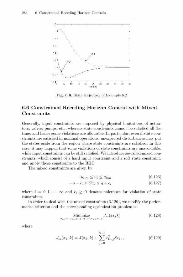
284 6 Constrained Receding Horizon Controls

Fig. 6.6. State trajectory of Example 6.2

6.6 Constrained Receding Horizon Control with MixedConstraints

Generally, input constraints are imposed by physical limitations of actua-tors, valves, pumps, etc., whereas state constraints cannot be satisfied all thetime, and hence some violations are allowable. In particular, even if state con-straints are satisfied in nominal operations, unexpected disturbances may putthe states aside from the region where state constraints are satisfied. In thiscase, it may happen that some violations of state constraints are unavoidable,while input constraints can be still satisfied. We introduce so-called mixed con-straints, which consist of a hard input constraint and a soft state constraint,and apply these constraints to the RHC.

The mixed constraints are given by

−ulim ≤ ui ≤ ulim (6.126)−g − εi ≤ Gxi ≤ g + εi (6.127)

where i = 0, 1, · · · ,∞ and εi ≥ 0 denotes tolerance for violation of stateconstraints.

In order to deal with the mixed constraints (6.126), we modify the perfor-mance criterion and the corresponding optimization problem as

Minimizeuk,··· ,uk+N−1,εk,··· ,εk+N−1

Jm(xk, k) (6.128)

where

Jm(xk, k) = J(xk, k) +N−1∑j=0

εTk+jSεk+j (6.129)

6.6 Constrained Receding Horizon Control with Mixed Constraints 285

subject to

−ulim ≤ uk+j ≤ ulim, j = 0, 1, · · · , N − 1 (6.130)−g − εk+j ≤ Gxk+j ≤ g + εk+j , j = 0, 1, · · · , N − 1 (6.131)

where J(xk, k) is given in (6.94) and S > 0 is a weighting matrix for violationon state constraints. The constraints (6.126) and (6.130) are hard constraints,whereas the constraints (6.127) and (6.131) are soft constraints. They togetherare called mixed constraints if both exist. Note that the additional cost isincluded so as to penalize a measure of the state constraints violation. Werequire that uk+j = Hxk+j is applied for j ≥ N and the state trajectorysatisfies

−ulim ≤ Hxk+j ≤ ulim (6.132)−g ≤ Gxk+j ≤ g (6.133)

for j = N, · · · ,∞.It is shown that the cost monotonicity condition for a hard constraint still

holds under a specific condition for (6.126).u1

i and ε1i are optimal for J(xτ , τ, σ + 1), and u2i and ε2i are optimal for

J(xτ , τ, σ). If we replace u1i and ε1i by u2

i and ε2i up to σ − 1, and we useu1

σ = −Hxσ at time σ, then by the optimal principle we have

J∗(xτ , σ + 1) =σ∑

i=τ

[x1Ti Qx1

i + u1Ti Ru1

i + ε1Ti Sε1i ] + x1T

σ+1Qfx1σ+1

≤σ−1∑i=τ

[x2Ti Qx2

i + u2Ti Ru2

i + ε2Ti Sε2i ] + x2T

σ Qx2σ + x2T

σ HT RHx2σ

+ x2Tσ (A − BH)Qf (A − BH)x2

σ (6.134)

where xσ+1 = (A − BH)xσ.If xσ satisfies the condition (6.133), then the optimal value of εσ must be

zero. How to make xσ satisfy (6.133) will be discussed later. It follows from(6.134) that

δJ∗(xτ , σ) = J∗(xτ , σ + 1) − J∗(xτ , σ) (6.135)

=σ∑

i=τ

[x1Ti Qx1

i + u1Ti Ru1

i + ε1Ti Sε1i ] + x1T

σ+1Qfx1σ+1

−σ−1∑i=τ

[x2Ti Qx2

i + u2Ti Ru2

i + ε1Ti Sε1i ] − x2T

σ Qfx2σ

≤ x2Tσ Qx2

σ + x2Tσ HT RHx2

σ + x2Tσ (A − BH)Qf (A − BH)x2

σ

− x2Tσ Qfx2

σ

= x2Tσ Q + HT RH + (A − BH)T Qf (A − BH) − Qfx2

σ ≤ 0 (6.136)

286 6 Constrained Receding Horizon Controls

Finally, we have the cost monotonicity condition:

Q + HT RH + (A − BH)T Qf (A − BH) − Qf ≤ 0 (6.137)

In order to consider the cost function of a state constraint violation, we in-troduce the variable γ3 as

ETk SNEk < γ3 (6.138)[

γ3 ETk

Ek S−1N

]> 0 (6.139)

where Ek = [εk, · · · , εk+N−1]T and SN = diagS, · · · , S︸ ︷︷ ︸N

.

Finally, we have the following LMI problem:

Minγ1,γ2,γ3,Uk,εγ1 + γ2 + γ3 (6.140)

subject to (6.81), (6.98), (6.111), (6.139), (6.112), (6.113), (6.114).If there is a solution to the optimization problem (6.140), then it satisfies

all the conditions (6.126), (6.132), (6.133), and (6.137).

6.7 Constrained Output Feedback Receding HorizonControl

Constrained Output Feedback Receding Horizon Control with aDisturbance Invariant Set

We will show that an output feedback RHC guarantees the closed-loop sta-bility for a constrained system under some conditions. Since the system withconstraints is nonlinear, we cannot apply the separation principle to prove thestability of the system.

We consider the following system with input, systems disturbance, andmeasurement disturbance constraints:

xk+1 = Axk + Buk + Gwk (6.141)yk = Cxk + vk (6.142)

where

−ulim ≤ uk ≤ ulim

−vlim ≤ vk ≤ vlim

−wlim ≤ wk ≤ wlim

(6.143)

The state is not accessible and an observer of the plant

xk+1 = Axk + Buk + L(yk − Cxk) (6.144)

6.7 Constrained Output Feedback Receding Horizon Control 287

is used to provide estimated states instead. The dynamics of the state esti-mation error ek = xk − xk can be derived as

ek+1 = (A − LC)ek + Gwk − Lvk (6.145)

It is assumed that the bounds on the initial estimation error are given as

|e0| ≤ e0 (6.146)

By combining (6.144) and (6.145), it is possible to build the following aug-mented system:

xak+1 =

[A LC0 A − LC

]xa

k +[

B0

]uk +

[0 LG −L

]da

k (6.147)

where

xak =

[xT

k eTk

]T, da

k =[wT

k vTk

]T (6.148)

It is assumed that the control uk is represented as

uk = Fxk + νk (6.149)

where νk is an additional control which will be explained later. F in (6.149)and L in (6.145) are chosen so that A − BF and A − LC respectively areHurwitz and meet a certain performance. Then, (6.147) can be rewritten as

xak+1 =

[ΦF LC0 ΦL

]xa

k +[

B0

]ck +

[0 LG −L

]da

k

= Φxak +[

B0

]ck + Ξda

k (6.150)

where ΦF = A + BF , ΦL = A − LC, and

Φ =[

ΦF LC0 ΦL

], Ξ =

[0 LG −L

](6.151)

Now, we set νk to zero and introduce a disturbance invariant set where alltrajectories satisfy the constraint once the initial state comes inside.

For the matrix A ∈ m×n, |A| is defined as a matrix each of whose elementsis |Aij |. The following disturbance invariance set is considered:

EW,α = xak ∈ 2n| |Wxa

k| ≤ α, 0 < α ∈ 2n (6.152)

with a weighting symmetric matrix W that is a block diagonal matrix suchas

W =[

W1 00 W2

](6.153)

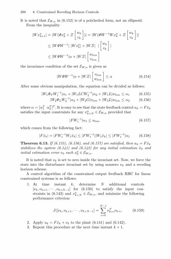
288 6 Constrained Receding Horizon Controls

It is noted that EW,α in (6.152) is of a polyhedral form, not an ellipsoid.From the inequality

|Wxak+1| = |W (Φxa

k + Ξ

[wk

vk

])| = |W (ΦW−1Wxa

k + Ξ

[wk

vk

])|

≤ |WΦW−1| |Wxak| + |WΞ| |

[wk

vk

]|

≤ |WΦW−1|α + |WΞ|[

wlim

vlim

]the invariance condition of the set EW,α is given as

|WΦW−1|α + |WΞ|[

vlim

wlim

]≤ α (6.154)

After some obvious manipulation, the equation can be divided as follows:

|W1ΦF W−11 |α1 + |W1LCW−1

2 |α2 + |W1L|wlim ≤ α1 (6.155)|W2ΦLW−1

2 |α2 + |W2G|vlim + |W2L|wlim ≤ α2 (6.156)

where α = [αT1 αT

2 ]T . It is easy to see that the state feedback control uk = Fxk

satisfies the input constraints for any xak+N ∈ EW,α provided that

|FW−11 |α1 ≤ ulim (6.157)

which comes from the following fact:

|Fxk| = |FW−11 W1xk| ≤ |FW−1

1 ||W1xk| ≤ |FW−11 |α1 (6.158)

Theorem 6.13. If (6.155), (6.156), and (6.157) are satisfied, then uk = Fxk

stabilizes the system (6.141) and (6.142) for any initial estimation x0 andinitial estimation error e0 such xa

0 ∈ EW,α.

It is noted that νk is set to zero inside the invariant set. Now, we force thestate into the disturbance invariant set by using nonzero νk and a recedinghorizon scheme.

A control algorithm of the constrained output feedback RHC for linearconstrained systems is as follows:

1. At time instant k, determine N additional controls[νk, νk+1, · · · , νk+N−1] for (6.150) to satisfy the input con-straints in (6.143) and xa

k+N ∈ EW,α, and minimize the followingperformance criterion:

J([νk, νk+1, · · · , νk+N−1] =N−1∑i=0

νTk+iνk+i (6.159)

2. Apply uk = Fxk + νk to the plant (6.141) and (6.142).3. Repeat this procedure at the next time instant k + 1.

6.8 References 289

It is noted that the above approach provides the stabilizing output feedbackcontrol and tends not to much deviate from the trajectory generated from thecontrol (6.149) with the observer (6.145).

The disturbance invariant set can be designed once or repeatedly eachtime. In the first case, as in dual-mode controls, the control is switched to thelinear output feedback control when the state enters the disturbance invariantset. In the second case, the disturbance invariance set is designed repeatedlyfor a better performance, which will be given as a problem in Section 6.9.

Constrained Linear Quadratic Finite Memory Control

It is shown that LQFMC can easily handle input constraints just by addingLMIs. Assume that the system matrix A is nonsingular and the following LMIproblem is feasible:

minF,W

tr(W )

subject to[W R

12 (FMT + H0)

(FMT + H0)T R12 (GNf

QNfGT

Nf+ RNf

)−1

]> 0 (6.160)

−ulim ≤ HYk−1 − HBNfUk−1 ≤ ulim (6.161)

where H0 = −K1(CTNf

CNf)−1CNf

and the columns of MT consist of the basisof the null space of CT

Nf. Then the gain matrices of the constrained LQFMC

is given byH = FMT + H0, L = −HBNf

It is noted that inequalities (6.161) are of an LMI form, which decreases thefeasibility.

6.8 References

Reachable sets and maximal output admissible sets in Section 6.2 are mostlybased on [BGFB94] and [GT91] respectively. In particular, constrained LQcontrols in Section 6.2 using a maximal admissible set appeared in [KG88][SR98].

The cost monotonicity for the fixed terminal case (xk+N = 0) in The-orem 6.2 and the stability of the RHC in Theorem 6.3 hold for nonlinearand constrained systems, which can be easily proved from well-known resultswithout the help of any references. The stability in the case of a zero termi-nal constraint in Theorem 6.3 appeared in [MM93] for constrained nonlinearsystems.

290 6 Constrained Receding Horizon Controls

The invariant ellipsoid for the linear state feedback control in Lemma 6.4and the feasibility of a solution in Theorem 6.5 appeared in [LKC98]. Thefinite arriving time to the invariant set in Theorem 6.6 is a discrete-timeversion of [MM93].

The constrained receding horizon control in Theorem 6.7 appeared in[LKC98]. A cost monotonicity condition for constrained systems in Theorem6.8 and its stability in Theorem 6.9 appeared in [LKC98]. The stability of alinear feedback control for linear unconstrained systems in Theorem 6.10 ap-peared in [LKC98] without a proof. The property of an invariant ellipsoid inTheorem 6.11 and an LMI representation for the constrained RHC in Theo-rems 6.12 appeared in [LKC98]. The RHC with a mixed constraint in Section6.6 is based on [ZM95].

The constrained output feedback RHC in Theorem 6.13 appeared in[LK01]. The disturbance invariant set in Section 6.7 is introduced in [KG98][Bla91], and how to find it for the dynamic equation (6.147) is dealt with in[LK99].

6.9 Problems

6.1. Consider the system (6.1) with∑N−1

i=0 uTi ui ≤ 1.

(1) Show that (xN − ANx0)T (WWT )−1(xN − ANx0) ≤ 1, where W =[AN−1B · · ·B].

(2) If A and B are given by

A =[

0.9746 0.1958−0.1953 0.5839

], B =

[0.8831−0.8811

](6.162)

compute P satisfying the LMI (6.14).(3) The ellipsoid (6.15) made by P contains the reachable set. Check whether

WWT ≤ P−1 for the system (6.162).

6.2. Show that the maximal output admissible set is positively invariant.

6.3. Suppose that a system and an off-origin ellipsoid are given by

xk+1 = −12xk + uk

(xk − 0.5)2 ≤ α

Find α such that the ellipsoid is invariant with a linear stable feedback control.Additionally, compute the corresponding state feedback controller inside theellipsoid.

6.4. Consider polytopic uncertain systems [BGFB94] described by

xk+1 = Axk + Buk, − ui ≤ uk ≤ ui (6.163)

6.9 Problems 291

where x ∈ Rn, u ∈ Rm, and

(A, B) =np∑i=1

ηi(Ai, Bi), ηi ≥ 0,np∑i=1

ηi = 1

If we use a state feedback controller u = Fx and a state transformationx = V z, we get

zk+1 = Φzk, Φ = V −1(A + BF )V (6.164)

(1) Denote that |z| = |zi| and α is a positive column vector. Derive a nec-essary and sufficient condition to make the set

x ∈ Rn| |z| ≤ α (6.165)

be invariant with respect to the closed-loop dynamics of (6.164).(2) Derive a condition to make F robustly stabilizing.

6.5. Considering the following system with constraints on the state and input:

xi+1 =[

1 10 1

]xi +

[01

]ui (6.166)

where [−1−1

]≤ xi ≤

[11

], − 1 ≤ ui ≤ 1 (6.167)

Find the invariant set xT Px ≤ 1 and compute the corresponding state feed-back control which makes the state stay inside the terminal ellipsoid forever.

6.6. Consider the systems (2.287) and (2.288) in the second problem of Prob-lem 2.2. Obtain an RHC to minimize the performance criterion

J =3∑

j=0

0.5[x21,k+j + x2

2,k+j + u2k+j ] (6.168)

subject to x1,k+4 = x2,k+4 = 0. The control and states are constrained by(2.290) and (2.291).

6.7. Consider an RHC design problem with the minimum energy performancecriterion given by

J =k+N−1∑

i=k

uTi Rui (6.169)

subject to the system xk+1 = Axk +Buk and the equality constraint xk+N =0. Find the RHC uk satisfying the constraint |uk| ≤ uk.

292 6 Constrained Receding Horizon Controls

6.8. Consider a system represented as follows:

xi+1 =[

0.8676 −0.3764−0.0252 0.8029

]xi +

[−0.3764−0.8029

]ui (6.170)

where the initial state x0 is set to [1.2 0.3]T , and ui and xi should be con-strained in the following region:

−1 ≤ ui ≤ 1 (6.171)[−1.5−0.3

]≤ Gxi =

[1 00 1

]xi ≤

[1.50.3

](6.172)

Here, the following performance criterion is considered:

J(xk, k)=

4∑j=0

xTk+jxk+j + u2

k+j (6.173)

(1) Find P such that

EP,1 = x ∈ n|xT Px ≤ 1 (6.174)

is an invariant set with respect to some linear state feedback control.(2) Compute the constrained receding horizon dual-mode control for the ter-

minal set constraint (6.174).

6.9. Consider an RHC design problem with the following performance index:

J =4∑

i=0

(x21,k+i + x2

2,k+i + u2k+i) + xT

k+5Qfxk+5

with initial state x0 = [1.5 0.3]T subject to the systems and the constraints

x1,k+1 = −x1,k − 0.5x2,k

x2,k+1 = −1.2x2,k − x1,k + uk

−2 ≤ x1,k ≤ 2−2 ≤ x2,k ≤ 2−2 ≤ uk ≤ 2

(1) Find the condition on Qf satisfying the cost monotonicity.(2) Represent the condition in an LMI form such that the ellipsoid xk|xT

k Qfxk

≤ 1 is a positive invariance set with a linear state feedback controlleruk = Hxk.

(3) Obtain an RHC in an LMI form.

6.9 Problems 293

6.10. Under the conditions of Problem 2.6, consider an RHC design problemfor the system (2.302) with the following performance criterion:

J = βxk+N +N−1∑j=0

(xk+j − uk+j) (6.175)

(1) Derive the condition on β satisfying the cost monotonicity.(2) Check the stability of the closed-loop system controlled by the RHC.

6.11. (1) Find a condition on Qf satisfying the cost monotonicity for thefollowing system and performance criterion:

xk+1 =12xk + uk

J =N−1∑i=0

(x2k+i + u2

k+i) + xTk+NQfxk+N

Design an RHC in an LMI form under the following constraints:

−1 ≤ xk ≤ 1−1 ≤ uk ≤ 1

(2) Find a condition on Qf satisfying the cost monotonicity for the followingsystem and performance criterion:

x1,k+1 = x1,k +12x2,k

x2,k+1 = −ax1,k − bx2,k + cuk

J =N−1∑i=0

(x21,k+i + x2

2,k+i + u2k+i) + xT

k+NQfxk+N

Obtain an RHC in an LMI form under the following constraints:

−1 ≤ x1,k ≤ 1−1.5 ≤ x2,k ≤ 1.5−2 ≤ uk ≤ 2

6.12. Consider an RHC design problem for the system

xk+1 = Axk + Buk

with the following performance criterion:

J(xk, uk) =k+N−1∑

i=k

[xi

ui

]T [Q SST R

] [xi

ui

]+ xT

k+NQfxk+N

294 6 Constrained Receding Horizon Controls

(1) Derive a condition on Qf satisfying the cost monotonicity.(2) Design the RHC in an LMI form under the following constraints:

−x ≤ xk ≤ x

−u ≤ uk ≤ u

where x and u are given vectors.

6.13. Consider the following system:

xk+1 =[

0.9347 0.51940.3835 0.8310

]xk +

[−1.4462−0.7012

]uk +

[10

]wk

yk =[0.5 0.5

]xk + vk

Assume that input and disturbances are constrained to

−1 ≤ uk ≤ 1−0.05 ≤ wk ≤ 0.05−0.1 ≤ vk ≤ 0.1

and the bound on the initial estimation error is [0.2 0.2]T .

(1) When the state feedback law F and filter gain L are chosen to be LQ andKalman filter gains, obtain F and L.

(2) Find W and α to determine the disturbance invariance set.

(3) Design a constrained output feedback RHC and perform the simulation.

6.14. Consider the following system:

xk+1 = Axk + Buk + Gwk

and the following min-max problem:

J∗(xk0 , k0, k1) = minuk

maxwk

J(xk0 , k0, k1)

where

J(xk0 , k0, k1) =k1∑

k=k0

[xTk Qxk + uT

k Ruk − γ2wTk wk] + xT

k1Qfxk1

(1) Derive a condition on Qf to satisfy J∗(xk0 , k0, k1+1)−J∗(xk0 , k0, k1) ≤ 0.

(2) Let V (xk0 , N) = J∗(xk0 , k0, k1), where N = k1−k0. Show that V (xk0 , N) ≥0 for all xk0 .

6.9 Problems 295

(3) Show that V (0, N) = 0 under the condition of 1).

(4) Assume that wk ∈ W , xk ∈ X, and uk ∈ U , where

W = wk ∈ Rn| wTk Dwk ≤ 1

X = xk ∈ Rn| x− ≤ xk ≤ x+ U = uk ∈ Rm| u− ≤ uk ≤ u+

Consider the following ellipsoid set:

E = xk ∈ Rn|xTk Qfxk ≤ 1

Derive a condition on Qf to satisfy xTk+1Qfxk+1 ≤ xT

k Qfxk for all wk ∈ Wand all xk ∈ ∂E, the boundary of E.

(5) Show that the constrained RHC under conditions obtained in (1) and (4)guarantee the H∞ performance.

(6) Show that, in the case of wk = 0, the RHC scheme of (5) guaranteesasymptotic stability.

7

Nonlinear Receding Horizon Controls

7.1 Introduction

In real plants, control systems are often represented by nonlinear dynamic sys-tems. Inputs and some states may be unconstrained or constrained dependingon the system characteristics. Generally, the finite-time optimal controls canbe obtained more easily than infinite-time optimal controls. Since the reced-ing horizon controls are obtained repeatedly over the finite horizon, they maybe easier to obtain than the infinite-time optimal controls. The optimizationproblems over the finite horizon, on which the RHC is based, can be appliedto a broad class of systems, including nonlinear systems and time-delayedsystems. Thus, the RHC has the same broad applications even for nonlinearsystems.

Often, the optimal controls are given as open-loop controls. Since the re-ceding horizon control uses the first control on a horizon, it is automaticallya closed-loop control, i.e. a function of the the current state. The cost mono-tonicity conditions for nonlinear systems can be easily obtained as in linearsystems. The terminal cost function becomes a control Lyapunov function(CLF) under the cost monotonicity condition. In this chapter, cost mono-tonicity conditions for the nonlinear RHC will be investigated according to aterminal equality constraint, a free terminal cost and a terminal invariant setwith or without a free terminal cost. And it is also shown that the stabilitycan be guaranteed from this cost monotonicity condition. The receding hori-zon control provides a systematic way to design a stabilizing control. Recedinghorizon controls for nonlinear systems are possible not only for minimizationcriteria, but also for minimaximization criteria.

The organization of this chapter is as follows. In Section 7.2, the RHCwith a terminal equality constraint is introduced for nonlinear systems. Inparticular, a cost monotonicity condition is presented in order to guarantee theclosed-loop stability. In Section 7.3, the nonlinear RHC with a fixed terminalset is introduced. In Section 7.4, the nonlinear RHC with a free terminal costis introduced for unconstrained and constrained systems. We shall also show

298 7 Nonlinear Receding Horizon Controls

that the nonlinear RHC can be obtained under a quadratic cost function. InSection, 7.5, the nonlinear RHC with an infinite cost horizon is introduced. InSection 7.6, the minimax RHC is presented for the H∞ performance criterion.

7.2 Nonlinear Receding Horizon Control with TerminalEquality Constraint

We consider the following discrete time-invariant nonlinear system:

xi+1 = f(xi, ui) (7.1)

where the input and the state belong to

ui ∈ U ⊂ m (7.2)xi ∈ X ⊂ n (7.3)

f(·, ·) ∈ C2 is a nonlinear function describing the system dynamics, andf(0, 0) = 0. If U = m and X = n, the system (7.1) is called an “un-constrained system”. In the case of U m or X n, the system (7.1) withconstraints (7.2) and (7.3) is called a “constrained system”. For constrainedsystems, U is often taken as a compact set including the origin.

We try to minimize the performance criterion such as

J(xk, k, k + N) =N−1∑j=0

g(xk+j , uk+j) (7.4)

subject to the terminal equality constraint

xk+N = 0 (7.5)

where g(xk, uk) denotes an intermediate cost. We assume that

c1(‖(xk, uk)‖) ≤ g(xk, uk) ≤ c2(‖(xk, uk)‖) (7.6)

where c1, c2 : R+ → R+ are all strictly increasing functions with c1(0) =c2(0) = 0. Note that g(0, 0) = 0. xk+j and uk+j are the predicted state andcontrol at the current time k. xk+j and uk+j satisfy xk+j+1 = f(xk+j , uk+j)with constraints

uk+j ∈ U , j = 0, 1, · · · , N − 1 (7.7)xk+j ∈ X , j = 0, 1, · · · , N (7.8)

The optimal control which minimizes the performance criterion (7.4) is as-sumed to exist for every initial state xk ∈ X ⊂ n, which is defined asfollows:

7.2 Nonlinear Receding Horizon Control with Terminal Equality Constraint 299

U∗k = [u∗T

k , u∗Tk+1, · · · , u∗T

k+N−1]T (7.9)

Then, the receding horizon control law is represented by

u∗k =

[1 0 · · · 0

]U∗

k (7.10)

All controls uk+j on the horizon are obtained as the open-loop controls de-pending on xk. Since the receding horizon control uses the first control on thehorizon, it is automatically a closed-loop control because it is a function ofthe current state.

If there is a feasible solution for the system (7.1) with constraints (7.5),(7.7) and (7.8) at the initial time 0 and some horizon N ∗, then the next solu-tions are guaranteed to exist, since at least one feasible solution u[k+1,k+N ] =[u[k+1,k+N−1] 0] exists. We have the following general result on feasibility.

Lemma 7.1. If there is a feasible solution on [k0, k0 +N∗], then there existsa feasible solution on [k, k + N ] for all k ≥ k0 and all N ≥ N∗.

Theorem 7.2. If it is assumed that there is a feasible solution on [k, σ] forthe system (7.1) with constraints (7.5), (7.7), and (7.8), then the optimalperformance criterion J∗(xk, k, σ) does not increase monotonically as σ in-creases.

J∗(xk, k, σ + 1) ≤ J∗(xk, k, σ) (7.11)

Proof. This can be proved by contradiction. Assume that u1i and u2

i are opti-mal controls to minimize J(xτ , τ, σ + 1) and J(xτ , τ, σ) respectively. If (7.11)does not hold, then

J∗(xτ , τ, σ + 1) > J∗(xτ , τ, σ)

Replace u1i by u2

i up to σ − 1 and then u1i = 0 at i = σ. In this case, x1

σ = 0,u1

σ = 0, and thus x1σ+1 = 0 due to f(0, 0) = 0. Therefore, the cost for this

control is J(xτ , τ, σ +1) = J∗(xτ , τ, σ). Since this control may not be optimalfor J(xτ , τ, σ + 1), we have J(xτ , τ, σ + 1) ≥ J∗(xτ , τ, σ + 1), which impliesthat

J∗(xτ , τ, σ) ≥ J∗(xτ , τ, σ + 1) (7.12)

This is a contradiction. It is noted that if J∗(xk, k, σ) exists, then J∗(xk, k, σ+1) exists according to Lemma 7.1. This completes the proof.

Theorem 7.3. If it is assumed that there is a feasible solution for the system(7.1) with constraints (7.5), (7.7), and (7.8) at the initial time and somehorizon N∗, then the receding horizon control (7.10) is asymptotically stablefor all horizons N ≥ N∗.

300 7 Nonlinear Receding Horizon Controls

Proof. The optimal performance criteria for the current time and the nexttime are related as

J∗(xk, k, k + N) = g(x1k, u1

k) + J∗(xk+1, k + 1, k + N)≥ g(x1

k, u1k) + J∗(xk+1, k + 1, k + N + 1) (7.13)

from which we have

J∗(xk, k, k + N) − J∗(xk+1, k + 1, k + N + 1) ≥ l(x1k, u1

k) (7.14)

Since the optimal cost J∗(xk, k, k + N) does not increase monotonically astime increases and is lower bounded, J∗(xk, k, k + N) approaches a constantvalue, the limit value. g(xk, uk) is always positive, except for xk = 0 anduk = 0. Since the left-hand side in (7.14) approaches zero, g(xk, uk) shouldalso approach zero. Therefore, the closed-loop system is asymptotically stable.This completes the proof.

7.3 Nonlinear Receding Horizon Control with TerminalSet Constraints

Consider a receding horizon control of the time-invariant nonlinear systemsdescribed by (7.1). An RHC at the current state xk is obtained by solving thefollowing finite-horizon optimal control problem J(xk, k, uk+·, Nk) defined by

J(xk, k, uk+·, Nk) =Nk∑j=0

g(xk+j , uk+j) (7.15)

subject to the control constraint

uk+j ∈ U , xk+j ∈ X (7.16)

where j = 0, 1, 2, · · · , and U ⊂ m and X ⊂ n are compact subsets contain-ing the origin in its interior. It is noted that the horizon size Nk at time kdepends on the current time k, whereas the horizon size was fixed in previoussections. In this section, we include the control uk as an argument of the costfunction for a better understanding.

Since a solution to the finite horizon optimal control problem J(xk, k, uk+·,Nk) with a terminal equality constraint xk+Nk

= 0 rarely exists due to con-straints, we can relax this constraint to a fixed terminal set of the form

xk+Nk∈ E (7.17)

where E is a terminal set that is some neighborhood of the origin. The con-straint (7.17) is a terminal set constraint. If the terminal equality constraintis relaxed in this way, then the receding horizon control is more feasible, but

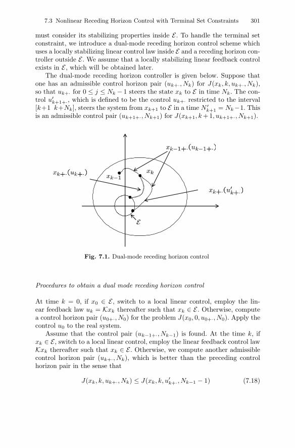
7.3 Nonlinear Receding Horizon Control with Terminal Set Constraints 301

must consider its stabilizing properties inside E . To handle the terminal setconstraint, we introduce a dual-mode receding horizon control scheme whichuses a locally stabilizing linear control law inside E and a receding horizon con-troller outside E . We assume that a locally stabilizing linear feedback controlexists in E , which will be obtained later.

The dual-mode receding horizon controller is given below. Suppose thatone has an admissible control horizon pair (uk+·, Nk) for J(xk, k, uk+·, Nk),so that uk+· for 0 ≤ j ≤ Nk − 1 steers the state xk to E in time Nk. The con-trol u′

k+1+·, which is defined to be the control uk+· restricted to the interval[k+1 k+Nk], steers the system from xk+1 to E in a time N ′

k+1 = Nk−1. Thisis an admissible control pair (uk+1+·, Nk+1) for J(xk+1, k +1, uk+1+·, Nk+1).

Fig. 7.1. Dual-mode receding horizon control

Procedures to obtain a dual mode receding horizon control

At time k = 0, if x0 ∈ E , switch to a local linear control, employ the lin-ear feedback law uk = Kxk thereafter such that xk ∈ E . Otherwise, computea control horizon pair (u0+·, N0) for the problem J(x0, 0, u0+·, N0). Apply thecontrol u0 to the real system.

Assume that the control pair (uk−1+·, Nk−1) is found. At the time k, ifxk ∈ E , switch to a local linear control, employ the linear feedback control lawKxk thereafter such that xk ∈ E . Otherwise, we compute another admissiblecontrol horizon pair (uk+·, Nk), which is better than the preceding controlhorizon pair in the sense that

J(xk, k, uk+·, Nk) ≤ J(xk, k, u′k+·, Nk−1 − 1) (7.18)

302 7 Nonlinear Receding Horizon Controls

where u′k+· is equal to the restriction of uk−1+· to the interval [k, k − 1 +

Nk−1] and is an admissible control for J(xk, k, uk+·, Nk). Finally, we applythe control uk to the real system.

(7.18) is necessary for a good performance. This is similar to the basicconcept of the existing receding horizon controllers which require the repeatedsolution of an optimal control problem.

Let X ∈ n denote the set of initial states which can be steered to E by acontrol in U . The above procedure is depicted in Figure 7.1.

The following procedure shows how to construct W. If the linearized sys-tem of (7.1) near the origin is stabilizable, then it can be shown that W isalways constructed. From the nonlinear system (7.1), we have the followinglinear system:

xi+1 = Axi + Bui (7.19)

where

A =∂f

∂x

∣∣∣∣x=0,u=0

B =∂f

∂u

∣∣∣∣x=0,u=0

(7.20)

By the assumption of the stabilizability, we can choose H such that A −BHis Hurwitz. f(xi,−Hxi) can be represented as

f(xi,−Hxi) = (A − BH)xi + φ(xi) = AHxi + φ(xi) (7.21)

Clearly, φ(xi) satisfies φ(0) = 0 and φ(xi)xi

→ 0 as xi approaches zero.Thus, for any 0 < κ < 1− ρ2(AH), AH√

1−κis Hurwitz and thus there exists

a P > 0 such that (AH√1 − κ

)T

P

(AH√1 − κ

)− P = −M (7.22)

for some positive definite matrix M . Letting P = P1−κ , it follows that

ATHPAH − (1 − κ)P = −M (7.23)

Additionally, there exists α1 such that

2xTi Pφ + φT Pφ ≤ κxT

i Pxi (7.24)

for all xi ∈ EP,α1 , where EP,α1 = x|xT Px ≤ α1, α1 > 0 since φ(xi)xi

→ 0.It is noted that input or state constraints must be satisfied in EP,α1 . As-

sume that there exists a region EP,α2 = x|xT Px ≤ α2, α2 > 0 such that−Hx ∈ U and x ∈ X for all x ∈ EP,α2 . The terminal region EP,α should beinside EP,α1 ∩ EP,α2 . This can be achieved numerically by adjusting α1 suchthat α1 ≤ α2.

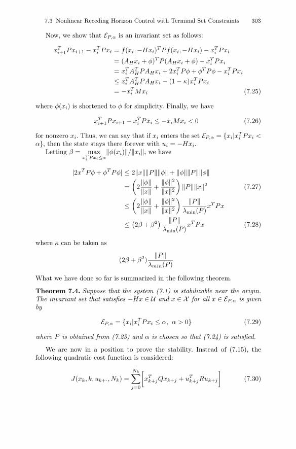
7.3 Nonlinear Receding Horizon Control with Terminal Set Constraints 303

Now, we show that EP,α is an invariant set as follows:

xTi+1Pxi+1 − xT

i Pxi = f(xi,−Hxi)T Pf(xi,−Hxi) − xTi Pxi

= (AHxi + φ)T P (AHxi + φ) − xTi Pxi

= xTi AT

HPAHxi + 2xTi Pφ + φT Pφ − xT

i Pxi

≤ xTi AT

HPAHxi − (1 − κ)xTi Pxi

= −xTi Mxi (7.25)

where φ(xi) is shortened to φ for simplicity. Finally, we have

xTi+1Pxi+1 − xT

i Pxi ≤ −xiMxi < 0 (7.26)

for nonzero xi. Thus, we can say that if xi enters the set EP,α = xi|xTi Pxi <

α, then the state stays there forever with ui = −Hxi.Letting β = max

xTi Pxi≤α

‖φ(xi)‖/‖xi‖, we have

|2xT Pφ + φT Pφ| ≤ 2‖x‖‖P‖‖φ‖ + ‖φ‖‖P‖‖φ‖

=(

2‖φ‖‖x‖ +

‖φ‖2

‖x‖2

)‖P‖‖x‖2 (7.27)

≤(

2‖φ‖‖x‖ +

‖φ‖2

‖x‖2

)‖P‖

λmin(P )xT Px

≤(2β + β2

) ‖P‖λmin(P )

xT Px (7.28)

where κ can be taken as

(2β + β2)‖P‖

λmin(P )

What we have done so far is summarized in the following theorem.

Theorem 7.4. Suppose that the system (7.1) is stabilizable near the origin.The invariant set that satisfies −Hx ∈ U and x ∈ X for all x ∈ EP,α is givenby

EP,α = xi|xTi Pxi ≤ α, α > 0 (7.29)

where P is obtained from (7.23) and α is chosen so that (7.24) is satisfied.

We are now in a position to prove the stability. Instead of (7.15), thefollowing quadratic cost function is considered:

J(xk, k, uk+·, Nk) =Nk∑j=0

[xT

k+jQxk+j + uTk+jRuk+j

](7.30)

304 7 Nonlinear Receding Horizon Controls

Theorem 7.5. Suppose that the linearized systems with respect to (7.1) isstabilizable. Then, for Nk > 1, there exists a control horizon pair (uk, Nk)such that the following equation is satisfied:

J(xk, k, uk, Nk) ≤ J(xk, k, u′k, Nk−1 − 1) (7.31)

and there exists constant 0 < η < ∞ satisfying

J(xk+1, k + 1, uk+1, Nk+1) ≤ J(xk, k, uk, Nk) − η (7.32)

for all k such that both xk and xk+1 are in EP,α.

Proof. The first statement is already explained in (7.18). Since the trajectoryby (uk, Nk) is the same as one by (uk+1, Nk − 1) on [k + 1, k + Nk], we have

J(xk, k, uk, Nk) − J(xk+1, k + 1, uk+1, Nk+1) (7.33)≥ J(xk, k, uk, Nk) − J(xk+1, k + 1, u′

k+1, Nk − 1) (7.34)

= xTk Qxk + uT

k Ruk (7.35)

≥ λmin(Q)λmax(P )

α = η (7.36)

for all k such that both xk and xk+1 lie in EP,α, as seen in Theorem 6.5. Thiscompletes the proof.

Theorem 7.6. The dual-mode receding horizon controller is asymptoticallystabilizing with a region of attraction X. For all x0 ∈ X, there exists a finitetime N∗ such that xN∗ ∈ EP,α.

Proof. The proof of this theorem is the same as Theorem 6.6

In this section, suboptimal controls satisfying (7.18) were considered. How-ever, we can even use optimal controls for the following performance criterion:

minui

N−1∑j=0

g(xk+j , uk+j) (7.37)

instead of (7.18). This requires heavier computation compared with subopti-mal controls, but provides better performance.

7.4 Nonlinear Receding Horizon Control with FreeTerminal Cost

We consider the discrete time-invariant nonlinear systems (7.1) and minimizea cost function such as

7.4 Nonlinear Receding Horizon Control with Free Terminal Cost 305

J(xk, k, k + N) =N−1∑j=0

g(xk+j , uk+j) + h(xk+N ) (7.38)

where h(·) is a terminal weighting function. We assume that

c3(‖x‖) ≤ h(x) ≤ c4(‖x‖)

where c3, c4 : R+ → R+ are all strictly increasing functions with c3(0) =c4(0) = 0. Note that h(0) = 0.

Theorem 7.7. Assume that there is a feasible solution for the system (7.1)with constraints (7.7) and (7.8). If the following inequality is satisfied:

g(xσ,K(xσ)) + h(f(xσ,K(xσ))) − h(xσ) ≤ 0 (7.39)

where xσ ∈ X , f(xσ,K(xσ)) ∈ X , and K(xσ) ∈ U , then the optimal perfor-mance criterion J∗(xk, k, σ) does not increase monotonically as σ increases,

J∗(xk, k, σ + 1) ≤ J∗(xk, k, σ) (7.40)

Proof. In the same way as Theorem 3.2, we can prove the nonincreasingmonotonicity of the optimal cost. u1

i and u2i are optimal controls to mini-

mize J(xk, k, σ + 1) and J(xk, k, σ) respectively. If we replace u1i by u2

i up toσ − 1 and u1

σ = K(xσ), then the cost for this control is given by

J(xk, σ + 1)=

σ−1∑j=k

g(x2j , u

2j ) + g(x2

σ,K(x2σ)) + h(x2

σ+1)

≥ J∗(xk, σ + 1) (7.41)

where the last inequality comes from the fact that this control may not beoptimal. The difference between the adjacent optimal costs is less than orequal to zero as

J∗(xk, σ + 1) − J∗(xk, σ) ≤ J(xk, σ + 1) − J∗(xk, σ)= g(x2

σK(x2σ)) + h(x2

σ+1) − h(x2σ) ≤ 0 (7.42)

where J∗(xk, σ) is given by

J∗(xk, σ) =σ−1∑j=k

g(x2j , u

2j ) + h(x2

σ) (7.43)

This completes the proof.

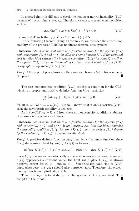
306 7 Nonlinear Receding Horizon Controls

It is noted that it is difficult to check the nonlinear matrix inequality (7.39)because of the terminal state, xσ. Therefore, we can give a sufficient conditionsuch as

g(x,K(x)) + h(f(x,K(x))) − h(x) ≤ 0 (7.44)

for any x ∈ X such that f(x,K(x) ∈ X and K(x) ∈ U .In the following theorem, using Theorem 7.7, we consider the closed-loop

stability of the proposed RHC for nonlinear discrete-time systems.

Theorem 7.8. Assume that there is a feasible solution for the system (7.1)with constraints (7.7) and (7.8) for all k and some horizon N ∗. If the terminalcost function h(x) satisfies the inequality condition (7.44) for some K(x), thenthe system (7.1) driven by the receding horizon control obtained from (7.38)is asymptotically stable for N ≥ N∗.

Proof. All the proof procedures are the same as Theorem 3.6. This completesthe proof.

The cost monotonicity condition (7.39) satisfies a condition for the CLF,which is a proper and positive definite function h(xk) such that

infuk

[h(xk+1) − h(xk) + g(xk, uk)

]≤ 0 (7.45)

for all xk = 0 and uk = K(xk). It is well known that if h(xk) satisfies (7.45),then the asymptotic stability is achieved.

As in the CLF, uk = K(xk) from the cost monotonicity condition stabilizesthe closed-loop systems as follows.

Theorem 7.9. Assume that there is a feasible solution for the system (7.1)with constraints (7.7) and (7.8). If the terminal cost function h(xk) satisfiesthe inequality condition (7.44) for some K(xk), then the system (7.1) drivenby the control uk = K(xk) is asymptotically stable.

Proof. A positive definite function h(xt) can be a Lyapunov function sinceh(xk) decreases at least by −g(xk,K(xk)) as follows:

h(f(xk,K(xk))) − h(xk) = h(xk+1) − h(xk) ≤ −g(xk,K(xk)) < 0 (7.46)

Since h(xk) decreases monotonically as time increases and is lower bounded,h(xk) approaches a constant value, the limit value. g(xk,K(xk)) is alwayspositive, except for xk = 0 and uk = 0. Since the left-hand side in (7.46)approaches zero, g(xk, uk) should also approach zero. Therefore, the closed-loop system is asymptotically stable.

Thus, the asymptotic stability for the system (7.1) is guaranteed. Thiscompletes the proof.

7.4 Nonlinear Receding Horizon Control with Free Terminal Cost 307

It is noted that the receding horizon control obtained from the cost mono-tonicity condition integrated with K(xk) is asymptotically stabilizing if a feed-back control law uk = K(xk) is also asymptotically stabilizing.

We now introduce a terminal invariant ellipsoid Wα which is defined as

Eh,α = xk ∈ X | h(xk) ≤ α K(xk) ∈ U , f(xk,K(xk)) ∈ X , α > 0 (7.47)

Once xk enters the terminal region Eh,α, the state trajectory due to uk =K(xk) would remain in Eh,α because h(xK

k+N+1) ≤ h(xk+N )−g(xk+N ,K(xk+N ))≤ α. Hence, the input and state constraints in (7.63) are all satisfied. We callEh,α an invariant terminal region. If there exists a control that steers the initialstate to Eh,α, then there exist feasible controls for all times since the feasiblecontrol at the time k can be one of the candidates of the feasible controls atthe next time k + 1. What we have done so far is summarized as follows.

Lemma 7.10. If there exists a control that steers the initial state to Eh,α,then there exist feasible controls for all times.

The optimization problem (7.38) can be transformed into

Minimizeγ1,γ2,K,h,Uk

γ1 + γ2

subject to⎧⎪⎪⎨⎪⎪⎩xk+j|k ∈ X , j = 0, 1, · · · , N − 1uk+j|k ∈ U , j = 0, 1, · · · , N − 1∑N−1

j=0 g(xk+j , uk+j) ≤ γ1,h(xk+N |k) ≤ γ2

(7.48)

where h(·) satisfies the inequality (7.44). Additionally, another constraint

γ2 ≤ α (7.49)

is required for introducing an invariant ellipsoid Eh,α such as (7.47). It isnoted that the problem (7.48) and (7.49) is slightly different from the originalproblem (7.38).

In the following theorem, we consider the closed-loop stability of the pro-posed RHC derived from (7.48) and (7.49) for nonlinear systems. Accordingto Lemma 7.10, Theorem 7.8 is changed to the following.

Theorem 7.11. If there exists a control that steers the initial state to Eh,α,then the system (7.1) with the receding horizon control obtained from (7.48)-and (7.49) is asymptotically stable.

In the case of constrained linear systems, the final weighting matrix Qf

can be obtained each time for good performance. However, in the case ofnonlinear systems it is not easy to find a final weighting function h(·) eachtime. Thus, we find h(·) once and then may use it thereafter. The conditionγ2 ≤ α is required so that Eh,γ2 has an invariance property, Eh,γ2 ⊂ Eh,α.

308 7 Nonlinear Receding Horizon Controls

If, at the first step, we can find a terminal region Eh,α and a control se-quence that steers the current state into Eh,α, then feasible solutions existthereafter. However, in order to obtain good performance such as fast conver-gence to zero, we will try to find the Eh,α each time. As Eh,α shrinks more andmore, the control makes the current state closer to the origin.

Figure 6.5 shows the state trajectory due to the RHC which stems from theoptimization (7.48) conceptually. In the proposed RHC, the state at the endof the horizon falls on the boundary of the terminal region Eh,min(α,γ2). Thisis because h, K, and Eh,min(α,γ2) are also free parameters for optimization.However, computing h, K, and Eh,min(α,γ2) at each time is not easy, especiallyfor nonlinear systems, due to the computational burden or the lack of a suit-able numerical algorithm. However, this can be done at least for constrainedlinear systems, using SDP as shown in Section 6.4.

Now, we consider the following quadratic cost function:

N−1∑j=0

[xT

k+jQxk+j + uTk+jRuk+j

]+xk+NQfxk+N (7.50)

for the nonlinear systems (7.1). In a quadratic cost function, the cost mono-tonicity condition (7.39) is changed to

fT (xk,−K(xk))Qff(xk,−K(xk)) − xTk Qfxk

≤ −xTk Qxk − uT

k Ruk (7.51)

In the previous section it was shown that the terminal cost function h(x) ischosen to be a CLF. However, to find K(x) and h(x) satisfying (7.39) is notso easy, as mentioned before.

Here, the cost function is given in a quadratic form as (7.50) and K(x) isa local linear state-feedback −Hx as shown in Section 6.5.

To obtain a local linear state-feedback control, we consider the Jacobianlinearization (7.19) of the system (7.1) at the origin where A and B are givenby (7.20). From A and B in (7.20), H is chosen such that 0 < ρ(A−BH) < 1,where ρ(·) is the spectral radius of a matrix.

Since h(x) = xT Qfx, the terminal region is represented by EQf ,α =x|xT Qfx ≤ α. How to determine α is given later in this section.

For any 0 < κ < 1 − ρ2(AH), it is noted that there exist matrices H andQf such that

ATHQf AH − Qf = −[Q + HT RH] (7.52)

where AH = A−BH√1−κ

, AH = A − BH, and Qf = Qf√1−κ

. Since ||φ||/||x|| → 0,there exists α1 such that

2xTk Qfφ + φT Qfφ ≤ κxT

k Qfxk (7.53)

for all xk ∈ EQf ,α1 , where EQf ,α1 = xk|xTk Qfxk ≤ α1, α1 > 0.

7.4 Nonlinear Receding Horizon Control with Free Terminal Cost 309

It is noted that input or state constraints must be satisfied in EQf ,α1 .Assume that there exists a region EQf ,α2 = xk|xT

k Qfxk ≤ α2, α2 > 0such that −Hxk ∈ U and xk ∈ X for all xk ∈ EQf ,α2 . The terminal regionEQf ,α should be inside (EQf ,α1 ∩EQf ,α2). This can be achieved numerically byadjusting α1 such that α1 ≤ α2.

Now we show that Qf in (7.52) satisfies the inequality (7.51) as follows:

f(xk,−Hxk)T Qff(xk,−Hxk) − xTk Qfxk

= (AHxk + φ)T Qf (AHxk + φ) − xTk Qfxk

= xTk AT

HQfAHxk + 2xTk Qfφ + φT Qfφ − xT

k Qfxk

≤ xTk AT

HQfAHxk − (1 − κ)xTk Qfxk

= −xTk (Q + HT RH)xk (7.54)

where φ(xk) is shortened to φ for simplicity.The cost monotonicity condition and the closed-loop stability of the non-

linear RHC is summarized in the following theorems.

Lemma 7.12. If Qf and EQf ,α are found out from (7.52) and (7.53), thenthe cost monotonicity condition (7.51) holds. In that case, the state startinginside EQf ,α remains in EQf ,α continuously with uk = −Hxk while satisfyingthe input and the state constraints.

Theorem 7.13. If Qf and EQf ,α are found out from (7.52) and (7.53), thereceding horizon control based on the cost function (7.50) asymptotically sta-bilizes the system (7.1) if it is feasible at the initial time.

Given Qf , the terminal region EQf ,α can be determined. The larger that αis, the smaller the control horizon N needed to stabilize the systems. Further-more, a smaller horizon leads to a lesser computational burden. Therefore, alarger α is preferable.

In the following, we give a numerical algorithm to decide a larger α. Thestate constraint X and the input constraint U are assumed as

−ulim ≤ ui ≤ ulim

−glim ≤ Gxi ≤ glim(7.55)

for i = 0, 1, · · · ,∞. It is guaranteed that the input and state constraints aresatisfied in the ellipsoid if the minimum values of the following optimizationproblems are all positive:⎧⎪⎪⎨⎪⎪⎩

min (ulim − Hxi)(i), i = 1, · · · ,mmin (ulim + Hxi)(i), i = 1, · · · ,mmin (glim − Gxi)(i), i = 1, · · · , n

min (glim + Gxi)(i), i = 1, · · · , n

(7.56)

subject to xi ∈ EQf ,α, where vi is an ith component of a vector v and EQf ,α =xi|xT

i Qfxi ≤ α, α > 0.

310 7 Nonlinear Receding Horizon Controls

The inequality (7.53) is satisfied if the minimum value of the followingoptimization problem is positive:

min κxTi Qfxi − 2xT

i Qfφi − φTi Qfφi

subject to xi ∈ EQf ,α

(7.57)

α is chosen so that the minimum values of optimization problems (7.56) and(7.57) are all positive simultaneously. If there is a negative minimum value,then we should decrease α and solve the optimization problem again. If theminimum values are all positive, then we increase α and solve the optimizationproblem to get a larger α.

Control Lyapunov Function-based Nonlinear Receding Horizon Con-tol:

A CLF can be combined with the receding horizon control. These controlschemes retain the global stability due to a Lyapunov function and the im-provement of the performance due to a receding horizon performance. TheCLF can be used with a one-step RHC. In this case, a control uk is obtainedby solving the following optimization problem:

min uTk uk (7.58)

subject to

h(xk+1) − h(xk) ≤ −σ(xk) (7.59)

where σ(xk) is a positive definite function. This scheme minimizes the controlenergy while requiring that h be a Lyapunov function for the closed-loopsystem and decrease by at least σ(xk) at every point, guarantee the stability.The CLF-based one-step RHC is extended to a general RHC based on theCLF such as

minN−1∑j=0

[l(xk+j) + uTk+juk+j ] (7.60)

subject to

h(xk+1) − h(xk) ≤ −σ(xk) (7.61)

Stability is guaranteed for any horizon N and the one-step RHC is recoveredif the horizon size N becomes 1. It is noted that the inequality (7.61) may beimposed over the horizon [k, k + N ] as

h(xk+1+j) − h(xk+j) ≤ −σ(xk+j) (7.62)

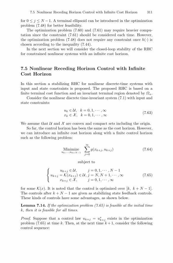
7.5 Nonlinear Receding Horizon Control with Infinite Cost Horizon 311

for 0 ≤ j ≤ N − 1. A terminal ellipsoid can be introduced in the optimizationproblem (7.48) for better feasibility.

The optimization problem (7.60) and (7.61) may require heavier compu-tation since the constraint (7.61) should be considered each time. However,the optimization problem (7.48) does not require any constraint once h(·) ischosen according to the inequality (7.44).

In the next section we will consider the closed-loop stability of the RHCfor constrained nonlinear systems with an infinite cost horizon.

7.5 Nonlinear Receding Horizon Control with InfiniteCost Horizon

In this section a stabilizing RHC for nonlinear discrete-time systems withinput and state constraints is proposed. The proposed RHC is based on afinite terminal cost function and an invariant terminal region denoted by Ωα.

Consider the nonlinear discrete time-invariant system (7.1) with input andstate constraints:

uk ∈ U , k = 0, 1, · · · ,∞xk ∈ X , k = 0, 1, · · · ,∞ (7.63)

We assume that U and X are convex and compact sets including the origin.So far, the control horizon has been the same as the cost horizon. However,

we can introduce an infinite cost horizon along with a finite control horizonsuch as the following problem:

Minimizeuk,...,uk+N−1

∞∑j=0

g(xk+j , uk+j) (7.64)

subject to⎧⎨⎩uk+j ∈ U , j = 0, 1, · · · , N − 1

uk+j = K(xk+j) ∈ U , j = N,N + 1, · · · ,∞xk+j ∈ X , j = 0, 1, · · · ,∞

(7.65)

for some K(x). It is noted that the control is optimized over [k, k + N − 1].The controls after k + N − 1 are given as stabilizing state feedback controls.These kinds of controls have some advantages, as shown below.

Lemma 7.14. If the optimization problem (7.65) is feasible at the initial timek, then it is feasible for all times.

Proof. Suppose that a control law uk+j = u∗k+j exists in the optimization

problem (7.65) at time k. Then, at the next time k +1, consider the followingcontrol sequence:

312 7 Nonlinear Receding Horizon Controls

uk+1|k+1 = uk+1|kuk+1+j|k+1 = u∗

k+1+j|k, j = 1, 2, · · · ,∞

(7.66)

Then, the above control sequence gives a feasible solution for the optimiza-tion problem (7.65) at time k + 1. Hence, by induction, if the optimizationproblem (7.65) is feasible at the initial time k = 0, then we observe that theoptimization problem is always feasible for all times k. This completes theproof.

The cost function (7.64) over the infinite cost horizon is divided into twoparts as follows:

∞∑j=0

g(xk+j , uk+j) =N−1∑j=0

g(xk+j , uk+j) +∞∑

j=N

g(xk+j , uk+j) (7.67)

=N−1∑j=0

g(xk+j , uk+j) + h(xk+N ) (7.68)

where

h(xk+N ) =∞∑

j=N

g(xk+j ,K(xk+j)) (7.69)

It is noted that xi for i ≥ k +N is the trajectory starting from xk+N with thestabilizing control ui = K(xi). As seen in Figure 7.2, the cost function for thefinal state represents one incurred when the stabilizing controller is appliedfor the rest of the time after the end of the horizon. From (7.69) we have

Fig. 7.2. Cost function with infinite cost horizon

7.6 Nonlinear Receding Horizon Minimax Control with Free Terminal Cost 313

h(xk+N+1) − h(xk+N ) =∞∑

j=N+1

g(xk+j ,K(xk+j)) −∞∑

j=N

g(xk+j ,K(xk+j))

= −g(xk+N ,K(xk+N )) (7.70)

It follows finally that

h(xk+N+1) − h(xk+N ) + g(xk+N ,K(xk+N )) = 0 (7.71)

This is a special case of (7.44). Then, the RHC automatically stabilizes thesystem due to (7.71) only if input and state constraints are all satisfied. Resultsin previous sections can be applied to the nonlinear RHC for the infinite costhorizon owing to (7.68) and (7.71).

Calculation of h(xσ) in (7.69) requires the summation of the closed-loopsystem with the stabilizing controller ui = K(xi) over a possibly long period.For linear systems, this is easily obtained from the algebraic Lyapunov equa-tion, but for nonlinear systems no easily computable method exists, whichmay further increase the burden of online computation of (7.69).

7.6 Nonlinear Receding Horizon Minimax Control withFree Terminal Cost

We consider the nonlinear system

xi+1 = f(xi, ui, wi) (7.72)

In this section, the input and the state constraints are not assumed. The finitehorizon optimal differential game at time k consists of the minimization withrespect to ui, and the maximization with respect to wi of the cost function

J(xk, uk, wk, N) =N−1∑j=0

[l(xk+j , uk+j) − γ2q(wk+j)

]+h(xk+N ) (7.73)

For any state xk ∈ n, if a feedback saddle-point solution exists, then wedenote the solution as u∗(k + j, xk) and w∗(k + j, xk). In the following, theoptimal value will be denoted by J∗(xk, k, k+N). In the receding horizon con-trol, at each time k, the resulting feedback control at the state xk is obtainedby optimizing (7.73) and setting

uk = u∗(k, xk) (7.74)

Theorem 7.15. If the following inequality is satisfied for some K(xk) and allxk = 0:

l(xk,K(xk)) − γ2q(w∗(xk)) + h(f(xk,K(xk), w∗k)) − h(xk) < 0 (7.75)

314 7 Nonlinear Receding Horizon Controls

then the optimal cost decreases monotonically as follows:

J∗(xk, k, k + N + 1) − J∗(xk, k, k + N) ≤ 0 (7.76)

for all positive integer N .

Proof. Subtracting J∗(xk, k, k + N) from J∗(xk, k, k + N + 1) yields

J∗(xk, k, k + N + 1) − J∗(xk, k, k + N)

=N∑

j=0

[l(x1

k+j , u1k+j) − γ2q(w1

k+j)]+h(x1

k+N+1)

−N−1∑j=0

[l(x2

k+j , u2k+j) − γ2q(w2

k+j)]−h(x2

k+N ) (7.77)

where the pair u1k+j and w1

k+j is a saddle-point solution for J(xk, k, k+N +1)and the pair u2

k+j and w2k+j for J(xk, k, k+N). If we replace u1

k+j by u2k+j and

w2k+j by w1

k+j on [k k + N − 1], then the following inequalities are obtainedby J(u∗, w∗) ≤ J(u,w∗):

N∑j=0

[l(x1

k+j , u1k+j) − γ2q(w1

k+j)]+h(x1

k+N+1)

≤N−1∑j=0

[l(xk+j , u

2k+j) − γ2q(w1

k+j)]+l(xk+N , u2

k+N )

− γ2q(w1k+N ) + h(xk+N+1) (7.78)

where xi is a trajectory associated with u2i and w1

i , u1σ = K(xσ), and xk+N+1 =

f(xk+N ,K(xk+N )). By J(u∗, w∗) ≥ J(u∗, w), we have

N−1∑j=0

[l(x2

k+j , u2k+j) − γ2q(w2

k+j)]+h(x2

k+N+1)

≥N−1∑j=0

[l(xk+j , u

2k+j) − γ2q(w1

k+j)]+h(xk+N+1) (7.79)

By using the two inequalities (7.78) and (7.79), it follows from (7.77) that

J∗(xk, k, k + N + 1) − J∗(xk, k, k + N)≤ l(xk+N ,K(xk+N )) − γ2q(w1

k+N (xk+N )) ≤ 0

where the last inequality comes from (7.75). This completes the proof.

7.6 Nonlinear Receding Horizon Minimax Control with Free Terminal Cost 315

Under the cost monotonicity condition, we can show that the closed-loopsystem without disturbances is asymptotically stabilized by RH H∞ control.

Theorem 7.16. If the cost monotonicity condition (7.75) is satisfied, thenthe system (7.72) with the RH H∞ control (7.74) is asymptotically stabilizedin the case that there is no disturbance.

Proof. First, we show that the optimal cost decreases monotonically as follows:

J∗(xk, k, k + N) = l(xk, uk) − γ2q(wk) + J∗(x(k + 1; (xk, k, u∗k)), k + 1, k + N)

≥ l(xk, uk) + J∗(x3(k + 1; (xk, k, u∗k)), k + 1, k + N)

≥ l(xk, uk) + J∗(x3(k + 1; (xk, k, u∗k)), k + 1, k + N + 1)(7.80)

where uk is the receding horizon control at time k, x3k+1 is a state at time

k + 1 when wk = 0, and the last inequality comes from the cost monotonicitycondition (7.76). It can be easily seen that J∗(xk, k, k + N) is bounded belowas

J∗(xk, k, k + N) =N−1∑j=0

[l(xk+j , uk+j) − γ2q(wk+j)

]+h(xk+N )

≥N−1∑j=0

l(x3k+j , u

3k+j) + h(x3

k+N ) ≥ 0

where x3k+j and u3

k+j are the state and the input in the case that the dis-turbances on [k , k + N ] are all zero. Therefore, J(xk, k, k + N) is boundedbelow, J∗(xk, k, k + N) ≥ 0. J∗(xk, k, k + N) approaches a constant number.It follows from (7.80) that

l(xk, uk) −→ 0 as k −→ 0 (7.81)

which implies that xk goes to zero. This completes the proof.

Under the cost monotonicity condition, we can show that the H∞ perfor-mance bound is met.

Theorem 7.17. If the cost monotonicity condition (7.75) is satisfied, thenthe nonlinear minimax RH control (7.74) for the system (7.72) satisfies∑∞

k=0 l(xk, uk)∑∞k=0 q(wk)

≤ γ2 (7.82)

Proof. Subtracting J∗(xk, k, k + N) from J∗(xk+1, k + 1, k + N + 1) yields

J∗(xk, k, k + N) = l(xk, uk) − γ2q(wk) + J∗(xk+1, k + 1, k + N)≥ l(xk, uk) − γ2q(wk) + J∗(xk+1, k + 1, k + N + 1) (7.83)

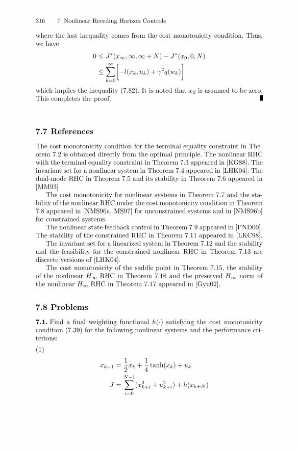
316 7 Nonlinear Receding Horizon Controls

where the last inequality comes from the cost monotonicity condition. Thus,we have

0 ≤ J∗(x∞,∞,∞ + N) − J∗(x0, 0, N)

≤∞∑

k=0

[−l(xk, uk) + γ2q(wk)

]which implies the inequality (7.82). It is noted that x0 is assumed to be zero.This completes the proof.

7.7 References

The cost monotonicity condition for the terminal equality constraint in The-orem 7.2 is obtained directly from the optimal principle. The nonlinear RHCwith the terminal equality constraint in Theorem 7.3 appeared in [KG88]. Theinvariant set for a nonlinear system in Theorem 7.4 appeared in [LHK04]. Thedual-mode RHC in Theorem 7.5 and its stability in Theorem 7.6 appeared in[MM93]

The cost monotonicity for nonlinear systems in Theorem 7.7 and the sta-bility of the nonlinear RHC under the cost monotonicity condition in Theorem7.8 appeared in [NMS96a, MS97] for unconstrained systems and in [NMS96b]for constrained systems.

The nonlinear state feedback control in Theorem 7.9 appeared in [PND00].The stability of the constrained RHC in Theorem 7.11 appeared in [LKC98].

The invariant set for a linearized system in Theorem 7.12 and the stabilityand the feasibility for the constrained nonlinear RHC in Theorem 7.13 arediscrete versions of [LHK04].

The cost monotonicity of the saddle point in Theorem 7.15, the stabilityof the nonlinear H∞ RHC in Theorem 7.16 and the preserved H∞ norm ofthe nonlinear H∞ RHC in Theorem 7.17 appeared in [Gyu02].

7.8 Problems

7.1. Find a final weighting functional h(·) satisfying the cost monotonicitycondition (7.39) for the following nonlinear systems and the performance cri-terions:

(1)

xk+1 =12xk +

14

tanh(xk) + uk

J =N−1∑i=0

(x2k+i + u2

k+i) + h(xk+N )

7.8 Problems 317

(2)

x1,k+1 = x1,k +12x2,k

x2,k+1 = −a sin(x1,k) − bx2,k + cuk

J(xk, k, k + N − 1) =N−1∑i=0

(x21,k+i + x2

2,k+i + u2k+i) + h(xk+N )

7.2. Consider a nonlinear RHC with a terminal equality constraint, xk+N = 0,for the following nonlinear system and the quadratic performance criterion:

xi+1 = f(xi, ui) = f1(xi) + f2(xi)ui (7.84)

and

J(xk, k, k + N − 1) =N−1∑i=0

(xTk+iQxT

k+i + uTk+iRuT

k+i) (7.85)

where R > 0 and Q > 0.

(1) Let fc(x) = f(x, k(x)) where k(x) is an RHC and fg(x) = f(x, φ(k(x)))where φ(x) is a function φ : p → p satisfying

φ(x)T Rφ(x) > (1 + α)(φ(x) − x)T R(φ(x) − x), ∀x = 0 (7.86)

and α is a real number such that

fT2 (x)

∂2J∗(βfc(x) + (1 − β)fg(x), k + 1, k + N − 1)∂x2

f2(x) ≤ αR(7.87)

for all x and 0 ≤ β ≤ 1. Show that J∗(f(xk, φ(k(xk))), k + 1, k + N −1) < J∗(xk, k, k + N − 1). Show that the closed-loop system with φ(·) isasymptotically stable.

(2) Assume that the function ψ : n → p satisfies xT Qx > 12 (1 +

α)ψT (x)Rψ(x) for x = 0. Show that J∗(f(xk, k(xk) + ψ(xk)), k + 1, k +N −1) < J∗(xk, k, k +N −1). Show that the closed-loop system with ψ(·)is asymptotically stable.

7.3. Consider the following nonlinear system:

x1,k+1 = x1,k − 0.5x2,k (7.88)x2,k+1 = −1.2x2,k + x1,k + x2

1,kx2,k + uk (7.89)

(1) Find a linearized model xk+1 = Axk + Buk around the origin and choosea feedback gain H such that A − BH is Hurwitz.

(2) For some κ satisfying 0 < κ < 1 − ρ2(A − BH), find P such that (A −BH)T P (A − BH) − (1 − κ)P = −I.

318 7 Nonlinear Receding Horizon Controls

(3) Find α such that (7.24) is satisfied in the positive invariant ellipsoidx|xT Px ≤ α.

7.4. Suppose that a system and an off-origin ellipsoid are given by

xk+1 = −12xk +

14x2

k + uk

(xk − 0.5)2 ≤ α

Find α such that the ellipsoid is invariant with a linear stable feedback control.Additionally, compute the corresponding state feedback controller inside theellipsoid.

7.5. (1) For the φi defined in (7.21), show that there exists a Ψ such that

|φi| ≤ Ψ |xi| (7.90)

where |v| of a vector v is |vi|.(2) For a given vector x, show that the set x ∈ n||xi| ≤ x is invariant if

(|A − BK| + Ψ)x < x.(3) For a given vector u, consider the following input constraint:

|u| ≤ u (7.91)

where |u| = |ui|. Find the condition to guarantee the feasibility whenthere is an input constraint.

7.6. Consider an RHC design problem with a free terminal cost. We assumethat a local stabilizing control law K, an associated Lyapunov function F , anda level set XF are known. More specifically, we assume that there exist K, F ,α > 0 such that

XF = x ∈ X |F (x) ≤ α (7.92)g(xσ,K(xσ)) + F (f(xσ,K(xσ))) − F (xσ) ≤ 0 (7.93)

Define

X0 = xk ∈ X |xk+N ∈ XF

The terminal cost is selected as

h(xk) :=

F (xk), xk ∈ XF

α, xk ∈ XF

(1) For each x0 ∈ X0, show that the closed-loop system by the control lawfrom the above RHC scheme is asymptotically stable.

(2) Show that X0 is invariant and a domain of attraction for the origin.

7.8 Problems 319

(3) If the assumption

F (xk) =∞∑

j=0

g(xk+j , uk+j), ∀xk ∈ X

is satisfied for all x0 ∈ XN , show that the RHC generates a control se-quence that solves the optimal control problem with the infinite horizonperformance index.

7.7. Consider a real system xk+1 = fr(xk, uk) and its model xk+1 = f(xk, uk).Assume that fr and f are twice continuously differentiable, ||fr(xk, uk) −f(xk, uk)|| ≤ β||(xk, uk)|| is satisfied, and f is Lipschitz continuous. Considerthe following linearized system of f with a local linear control law Kx:

xk+1 = Axk

where A = ∂f∂xk

(0, 0) + ∂f∂uk

(0, 0)K. We define P to satisfy

12xT

k Pxk =12

∞∑k=0

[xTk Qxk + xT

k KT RKxk]

For a given βL > 0, show that the set Wα = xk ∈ Rn|xTk Pxk ≤ α is

invariant if there exist an α > 0 and a K such that

xTk P [f(xk,Kxk) − Axk] − 1

2xT

k Qxk +λmin(P−1/2QP−1/2)

2xT

k Pxk

+βL[1 + ||K||P ]xTk Pxk ≤ 0

where || · ||P is a weighted norm.

7.8. Consider the following nonlinear system:

xk+1 = f(xk, uk)

with the performance index (7.38). The state and input vectors are subjectto the constraints xk ∈ X and uk ∈ U , where X and U are closed subsets ofRn and Rm respectively.

Assume

lim‖(xk,uk)‖ → 0

supk≥0

‖f(xk, uk)‖‖(xk, uk)‖ = 0

where f(xk, uk) = f(xk, uk) − [Akxk + Bkuk] and

A =∂f(xk, uk)

∂xk

∣∣∣∣xk=uk=0

, B =∂f(xk, uk)

∂uk

∣∣∣∣xk=uk=0

320 7 Nonlinear Receding Horizon Controls

(1) When a stable linear state feedback control law uk = Kxk for linearizedsystem is applied, the closed-loop system is given by

xk+1 = fc(xk) (7.94)

where fc(xk) = f(xk,Kxk). Let fc(x) = fc(xk) − [Ak + BkK]xk. Showthat

lim‖xk‖ → 0

supk≥0

‖fc(xk)‖‖xk‖

= 0

(2) In (7.38), assume that terminal cost is selected as

h(xk) =∑∞

j=k g(xcj,k,Kxc

j,k), xk ∈ X(K)∞, otherwise

where xcj,k is the solution of (7.94) at time j ≥ k when xk is given at time

k and X(K) is a stability region for the closed-loop system (7.94). Showthat the optimal performance index satisfies the following relations:

J∗(xk, k, k + N + 1) ≤ J∗(xk, k, k + N) (7.95)J∗(xk+1, k + 1, k + 1 + N) ≤ J∗(xk, k, k + N) (7.96)

(3) Show that the closed loop system controlled by the RHC is asymptoticallystable.

7.9. Consider a class of nonlinear systems:

xk+1 = f(xk, uk, wk) = a(xk) + b(xk)uk + g(xk)wk (7.97)

zk =[

h(xk)uk

](7.98)

We design an RHC based on the following min-max difference game:

V (xk, N) = minu

maxw

J(xk, N) (7.99)

where

J(xk, N) =N−1∑j=0

(||zk+j ||2 − γ2||wk+j ||2) + Vf (xk+N ) (7.100)

(1) Derive a condition on Vf such that

V (xk, N + 1) − V (xk, N) ≤ 0 (7.101)

(2) Under the condition of (1), if h(xk) ∈ K∞, then show that the closed-loopsystem is input-to-state stable with respect to wk, where K∞ is a set ofstrictly increasing functions with zero initial condition which approach ∞.

7.8 Problems 321

(3) Consider the following nonlinear discrete-time switched systems:

xk+1 = fp(xk, uk, wk), fp ∈ F (7.102)

where F = fp|p ∈ P indexed by the parameter p takes on values inthe set of parameters P which is either a finite set or a compact sub-set of some finite-dimensional, normed linear space. For each piece-wiseswitching signal as σ(·) : [0,∞) → P, we can define the switched non-linear systems xk+1 = fσ(xk, uk, wk). Also, we define the set of switchingtimes as T = k0, k1, k2, ... and assume Vf ∈ K∞. Using the result of (2)for each p, derive the condition to make the closed-loop switched systemscontrolled by the RHC satisfy

limi→∞

||xki|| = 0 (7.103)

(4) Using the results of (2) and (3) for each p, derive the condition to makethe closed-loop switched systems controlled by the RHC satisfy

limi→∞

||xi|| = 0 (7.104)

7.10. Consider the RHC design problem mentioned in Problem 7.9.

(1) Define J∗∞(x0) as the optimal cost of the infinite horizon difference game

with the following performance index:

J∞(x0) =∞∑

i=0

(||zi||2 − γ2||wi||2)

Show that

limk→∞

V (xk, N) = J∗∞(x0)

(2) Derive a condition to make the RHC guarantee a global stability result.

7.11. Consider the following nonlinear system and the performance criterion:

xk+1 =12xk +

14

tanh(xk) + wk (7.105)

J =N−1∑i=0

(x2k+i + u2

k+i − w2k+i) + h(xk+N ) (7.106)

Find a state feedback control K(xk) satisfying (7.75).

7.12. If h(xk) satisfies the following inequality:

h(xk) > minuk

maxwk

[l(xk)T l(xk) + uT

k uk − wTk wk

+ h(f(xk,K(xk), wk))]

(7.107)

then show that h(xk) also satisfies the inequality (7.75).

322 7 Nonlinear Receding Horizon Controls

7.13. Consider the input uncertainty in the nonlinear H∞ control (7.74), asshown in Figure 7.3. Assume that input uncertainty ∆ is given by

xk+1 = a(xk) + b(xk)uk (7.108)

yk = φ(xk) (7.109)

The input uk and output yk of the uncertainty ∆ satisfies

V(xk+1) − V(xk) ≤ uTk yk − ρuT

k uk

where V(xk) is some nonnegative function (this is called the dissipative prop-erty) and ρ ∈ R. Consider the following feedback interconnection with theinput uncertainty ∆:

uk = uRHCk

uk = −yk

Find the condition on ρ so that the closed-loop system has an H∞ norm boundγ for all dynamic input uncertainty ∆.

--

Fig. 7.3. Feedback interconnection of Problem 7.13

A

Matrix Equality and Matrix Calculus

A.1 Useful Inversion Formulae

The following relation is very useful even though it looks simple.

Theorem A.1. If (I + GK) is nonsingular, then the following relation issatisfied:

(I + GK)−1G = G(I + KG)−1 (A.1)

Proof.

(I + GK)−1G = G(I + KG)−1

←→ G(I + KG) = (I + GK)G←→ G + GKG = G + GKG

This completes the proof.

Theorem A.2. If it is assumed that A, C, and (A + BCD) are nonsingular,then we have the formula as

(A + BCD)−1 = A−1 − A−1B(DA−1B + C−1)−1DA−1 (A.2)

Proof. Multiplying the right side of (A.2) by A + BCD, we have

(A + BCD)[A−1 − A−1B(DA−1B + C−1)−1DA−1]= I + BCDA−1 − B(DA−1B + C−1)−1DA−1

− BCDA−1B(DA−1B + C−1)−1DA−1

= I + BCDA−1 − B(I + CDA−1B)(DA−1B + C−1)−1DA−1

= I + BCDA−1 − BC(C−1 + DA−1B)(DA−1B + C−1)−1DA−1 = I

Postmultiplying the right side of (A.2) by A+BCD, we have the same result.This completes the proof.

324 A Matrix Equality and Matrix Calculus

It is noted that Theorem A.2 is often called the matrix inversion lemma.

• The following matrix equality is obtained as

(I + GK)−1 = I − G(KG + I)−1K (A.3)= I − GK(GK + I)−1 (A.4)

by replacing A, B, C, and D by I, G, I, and K respectively in TheoremA.2. It is noted that the equality (A.4) comes from (A.1). Additionally, ifC in (A.2) is not invertible, then we can write

(A + BCD)−1 = A−1 − A−1B(CDA−1B + I)CDA−1 (A.5)

• The inverse of some matrices such as (I + KG) and (C−1 + DA−1B)is required on the right side of (A.1) and (A.2). It can be seen that thenonsingularity of I +GK implies that of I +KG in Theorem A.1. It is alsoshown in Theorem A.2 that the nonsingularity of (A+BCD) implies thatof (C−1 + DA−1B) under the assumption that A and C are nonsingular.The nonsingularity of these matrices is checked as follows:[

I 0−DA−1 I

] [A −BD C−1

] [I A−1B0 I

]=[

A 00 C−1 + DA−1B

](A.6)[

I BC0 I

] [A −BD C−1

] [I 0

−CD I

]=[

A + BCD 00 C−1

](A.7)

Using the product rule for determinants, the matrices decomposition in(A.6) and (A.7) give

det[

A −BD C−1

]= detAdet(C−1 + DA−1B) (A.8)

= detC−1 det(A + BCD) (A.9)

which tells us

det(C−1 + DA−1B) = 0 ⇐⇒ det(A + BCD) = 0 (A.10)

under the assumption that A and C are invertible. By replacing A, B, C,and D by I, G, I, and K respectively, it is also shown that the nonsingu-larity of I + GK implies that of I + KG in Theorem A.1.

In the following theorem, it is shown that matrices satisfying the equalityconstraint can be parameterized.

Theorem A.3. Suppose that A ∈ m×n is of full rank and n ≥ m. SolutionsX to the problem AX = Y can be parameterized as X = A⊥Y + MV forarbitrary matrices V , where A⊥ is the right inverse of A and M spans thenull space of A and its columns are orthogonal to each other. The number ofrows of V is equal to the dimension of the null space of A.

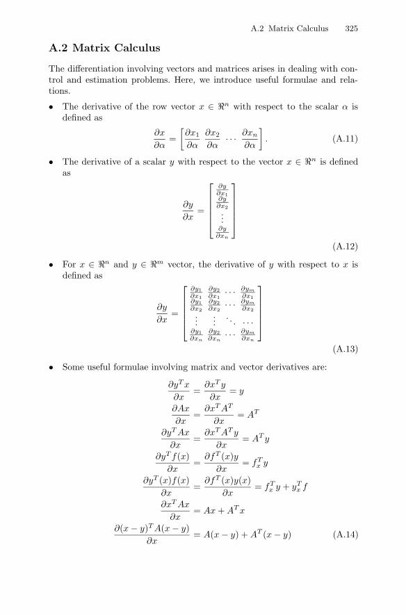
A.2 Matrix Calculus 325

A.2 Matrix Calculus

The differentiation involving vectors and matrices arises in dealing with con-trol and estimation problems. Here, we introduce useful formulae and rela-tions.

• The derivative of the row vector x ∈ n with respect to the scalar α isdefined as

∂x

∂α=[∂x1

∂α

∂x2

∂α· · · ∂xn

∂α

]. (A.11)

• The derivative of a scalar y with respect to the vector x ∈ n is definedas

∂y

∂x=

⎡⎢⎢⎢⎢⎣∂y∂x1∂y∂x2...

∂y∂xn

⎤⎥⎥⎥⎥⎦(A.12)

• For x ∈ n and y ∈ m vector, the derivative of y with respect to x isdefined as

∂y

∂x=

⎡⎢⎢⎢⎢⎣∂y1∂x1

∂y2∂x1

· · · ∂ym

∂x1∂y1∂x2

∂y2∂x2

· · · ∂ym

∂x2...

.... . . · · ·

∂y1∂xn

∂y2∂xn

· · · ∂ym

∂xn

⎤⎥⎥⎥⎥⎦(A.13)

• Some useful formulae involving matrix and vector derivatives are:

∂yT x

∂x=

∂xT y

∂x= y

∂Ax

∂x=

∂xT AT

∂x= AT

∂yT Ax

∂x=

∂xT AT y

∂x= AT y

∂yT f(x)∂x

=∂fT (x)y

∂x= fT

x y

∂yT (x)f(x)∂x

=∂fT (x)y(x)

∂x= fT

x y + yTx f

∂xT Ax

∂x= Ax + AT x

∂(x − y)T A(x − y)∂x

= A(x − y) + AT (x − y) (A.14)

326 A Matrix Equality and Matrix Calculus

If A is symmetrical, then simplified relations are obtained:

∂xT Ax

∂x= 2Ax

∂2xT Ax

∂x2= 2A

∂(x − y)T A(x − y)∂x

= 2A(x − y)

∂2(x − y)T A(x − y)∂x2

= 2A (A.15)

• The Hessian of a scalar function α with respect to a vector x is defined as

∂2α

∂x2=[

∂2α

∂xi∂xj

](A.16)

• The Taylor series expansion of a scalar function α(x) about x0 is

α(x) = α(x0) + (∂α

∂x)T (α − α0) +

12(α − α0)T (

∂2s

∂x2)T (α − α0)

+ terms of higher order (A.17)

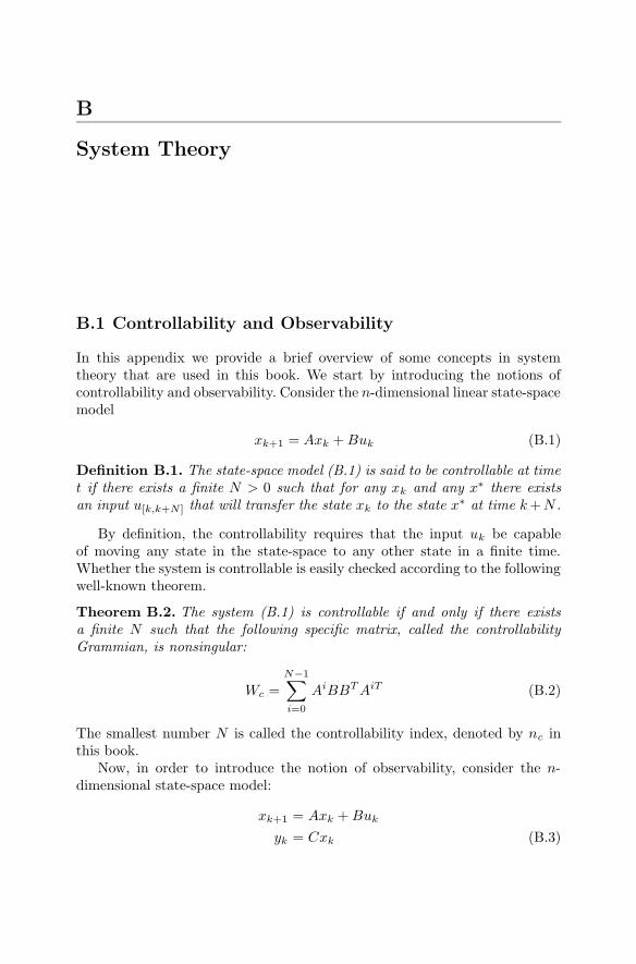
B

System Theory

B.1 Controllability and Observability

In this appendix we provide a brief overview of some concepts in systemtheory that are used in this book. We start by introducing the notions ofcontrollability and observability. Consider the n-dimensional linear state-spacemodel

xk+1 = Axk + Buk (B.1)

Definition B.1. The state-space model (B.1) is said to be controllable at timet if there exists a finite N > 0 such that for any xk and any x∗ there existsan input u[k,k+N ] that will transfer the state xk to the state x∗ at time k +N .

By definition, the controllability requires that the input uk be capableof moving any state in the state-space to any other state in a finite time.Whether the system is controllable is easily checked according to the followingwell-known theorem.

Theorem B.2. The system (B.1) is controllable if and only if there existsa finite N such that the following specific matrix, called the controllabilityGrammian, is nonsingular:

Wc =N−1∑i=0

AiBBT AiT (B.2)

The smallest number N is called the controllability index, denoted by nc inthis book.

Now, in order to introduce the notion of observability, consider the n-dimensional state-space model:

xk+1 = Axk + Buk

yk = Cxk (B.3)

328 B System Theory

Definition B.3. The system (B.3) is said to be observable at k if there existsa finite N such that the knowledge of the input u[k,k+N ] and the output y[k,k+N ]

over the time interval [k, k + N ] uniquely determines the state xk.

We have the following well known theorem.

Theorem B.4. The system (B.3) is observable at time k if and only if thereexists a finite N such that the following matrix observability Grammian isnonsingular:

Wo =N−1∑i=0

AiT CT CAi (B.4)

The smallest number N is called the observability index, denoted by no inthis book.

Note that observability is dependent only on A and C. The following the-orem shows the invariance of the observability.

Theorem B.5. The observability of (A,C) implies that of (A−BH,L) whereCT C + HT RH = LT L.

Proof: From the observability condition,

rank([

λI − AC

]) = n

for any real λ, is satisfied. Since the addition of a row vector does not changethe rank for full rank matrices, the rank of the following matrix is preserved:

rank(

⎡⎣λI − AC

R12 H

⎤⎦) = n.

If the third-row block is added to the first-row block with a pre-multiplicationby BR− 1

2 , the above matrix is changed as

rank(

⎡⎣λI − A + BHC

R12 H

⎤⎦) = n.

From the fact that rank(V ) = n with V ∈ n×m and n ≥ m impliesrank(V T V )=n,

rank(

⎡⎣λI − A + BHC

R12 H

⎤⎦T ⎡⎣λI − A + BHC

R12 H

⎤⎦) = n,

rank([

λI − A + BHL

]T [λI − A + BH

L

]) = n,

rank([

λI − A + BHL

]) = n.

B.1 Controllability and Observability 329

Therefore, (A − BH, L) is observable. This completes the proof.

The method of adjoint equations has been used in the study of terminalcontrol problems. In addition, the duality between control and estimation canbe precisely defined in terms of the adjoint system.

Suppose G : S1 → S2 is a linear system and S1 and S2 are Hilbert spaces.The adjoint system is a linear system G∗ : S2 → S1 that has the property

< Gw, y >S2=< w,G∗y >S1 (B.5)

for all w ∈ S1 and all y ∈ S2. To determine the adjoint of G in the Hilbertspace l2[0 k], consider inputs w ∈ l2[0 k] and represent the linear systemz = Gw by

zk =k∑

i=0

Gk−iwi (B.6)

For any y ∈ l2[0 k],

< Gw, y >=k∑

j=0

j∑i=0

ykGj−iwi =k∑

j=0

j∑i=0

(GTj−iyk)T wi =< w, η > (B.7)

where

ηj =j∑

i=0

GTj−iyk (B.8)

The l2[0 k] adjoint of G is therefore the system G∗ defined by

(G∗y)j =j∑

i=0

GTj−iyk (B.9)

In the case of a state-space system,

Gj−k = CAj−kB (B.10)

and it is easily shown that ηj =∑j

i=0 GTj−iyk satisfies

pi+1 = AT pi + CT yi (B.11)ηi = BT pi (B.12)

which is therefore a state-space realization of the adjoint system G∗.

330 B System Theory

B.2 Stability Theory

Here, we give some definitions on stability, attractivity, asymptotic stability,uniformly asymptotic stability, and exponential stability.

Consider the following nonlinear discrete time-varying system:

xi+1 = f(xi) (B.13)

where xi ∈ n and f(·) : n → n for all i ≥ i0. The solution evaluatedat the ith time with the initial time i0 and the initial state x0 is denoted byx(i; i0, x0).

A point xe ∈ n is called an equilibrium of the system (B.13), if

f(xe) = xe, ∀i ≥ i0

Definition B.6. (Stability) The equilibrium xe of the system (B.13) is stableif, for each ε > 0 and each i0 ≤ 0, there exists a δ = δ(ε, i0) such that

||x0|| < δ(ε, i0) → ||s(i, i0, i0)|| < ε, ∀i ≥ i0

Definition B.7. (Attractivity) The equilibrium xe is attractive if, for eachk0 ≥ 0, there exists an η(k0) such that

||x0|| < η(i0) → ||s(i, i0, i0)|| → 0 as i → ∞

Definition B.8. (Asymptotic stability) The equilibrium xe is asymptoticallystable if it is stable and attractive.

Definition B.9. (Exponential stability) The equilibrium xe is exponentiallystable if there exist constants η, a > 0 and p < 1 such that

||x0|| < η, i0 ≥ 0 → ||s(i0 + i, i0, i0)|| ≤ a||x0||pi, ∀i ≥ 0

Theorem B.10. (Lyapunov theorem) Suppose that V1, V2: + → + arecontinuous nondecreasing functions such that V1(s) and V2(s) are positive fors > 0 and V1(0) = V2(0) = 0. If there exists a continuous function V : n →+ satisfying

V1(‖x‖) ≤ V (x) ≤ V2(‖x‖) (B.14)

then the system is asymptotically stable.

Theorem B.11. (LaSalle’s theorem) Let Ω ⊂ D be a compact set that ispositively invariant with respect to the system xk+1 = f(xk). Let V : D → Rbe a function such that Vk+1 − Vk ≤ 0 in Ω. Let E be the set of all points inΩ where Vk+1 − Vk = 0. Let M be the largest invariant set in E. Then everysolution starting in Ω approaches M as t → ∞.

B.3 Lyapunov and Riccati Matrix Equations 331

B.3 Lyapunov and Riccati Matrix Equations

Lyapunov and Riccati equations arise in many contexts in linear systems the-ory. The characteristics of the two equations are summarized in this appendix.

Lyapunov Matrix Equation

We consider the following linear matrix equation, called a Lyapunov equa-tion:

K − AT KA = Q (B.15)

where Q is symmetric. If K exists and is unique, then K should be symmetric.

Theorem B.12. The Lyapunov equation (B.15) has the following properties:

(1)A unique solution K exists if and only if λi(A)λj(A) = 1 for all i and j.(2) If A is a stable matrix, then a unique solution K exists and can be expressed

as

K =∞∑

i=0

AiT QAi (B.16)

(3) If A is a stable matrix and Q is positive (semi) definite, then the uniquesolution K is positive (semi) definite.

(4) If A is a stable matrix, Q = CT C is positive semidefinite, and the pairA,C is observable, then the unique solution K is positive definite.

(5) Suppose that Q = CT C is positive semidefinite and the pair A,C isobservable. A is a stable matrix if and only if the unique solution K ispositive definite.

Proof. We prove only the fifth statement.(⇐=)Consider V (xi) = xT

i Kxi. Then we have

V (xi+1) − V (xi)= xT

i+1Kxi+1 − xTi Kxi (B.17)

= xTi (AT KA − K)xi = −xT

i Qxi ≤ 0 (B.18)

along any trajectory of xi+1 = Axi.We show that if Q is positive semidefinite and A,C is observable, then

xTi Qxi cannot be identically zero along any nontrivial trajectory of xi+1 =

Axi, which is proved as follows. Since

xTi Qxi = xT

0 AiT CT CAix0 = ‖CAix0‖2 (B.19)

and A,C is observable, all rows of CAi are linearly independent and thusCAix0 = 0 for all i = 0, 1, 2, · · · if and only if x0 = 0. By Lasalle’s theorem,

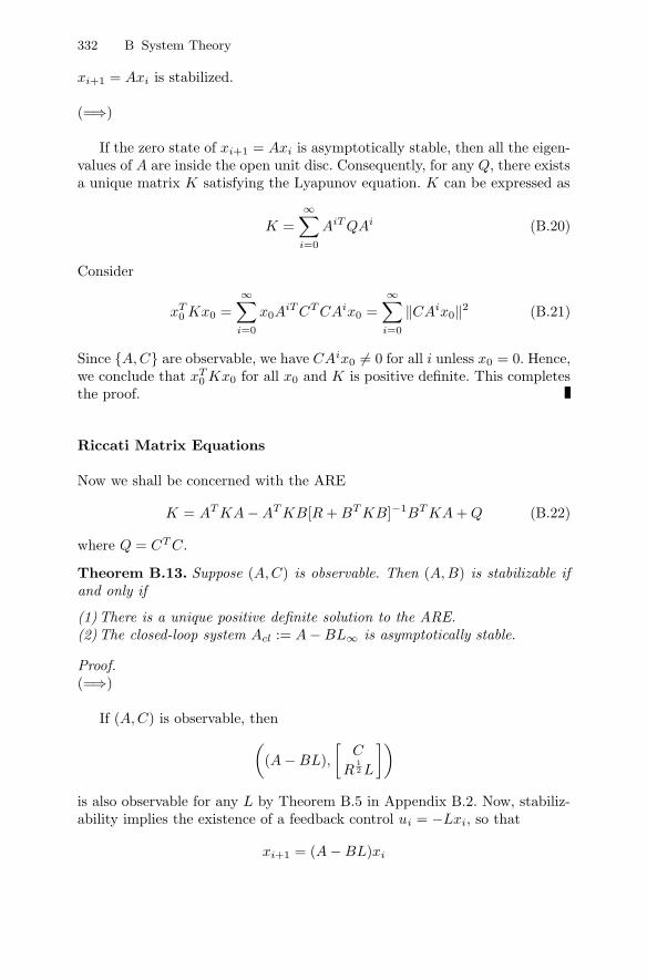
332 B System Theory

xi+1 = Axi is stabilized.

(=⇒)

If the zero state of xi+1 = Axi is asymptotically stable, then all the eigen-values of A are inside the open unit disc. Consequently, for any Q, there existsa unique matrix K satisfying the Lyapunov equation. K can be expressed as

K =∞∑

i=0

AiT QAi (B.20)

Consider

xT0 Kx0 =

∞∑i=0

x0AiT CT CAix0 =

∞∑i=0

‖CAix0‖2 (B.21)

Since A,C are observable, we have CAix0 = 0 for all i unless x0 = 0. Hence,we conclude that xT

0 Kx0 for all x0 and K is positive definite. This completesthe proof.

Riccati Matrix Equations

Now we shall be concerned with the ARE

K = AT KA − AT KB[R + BT KB]−1BT KA + Q (B.22)

where Q = CT C.

Theorem B.13. Suppose (A,C) is observable. Then (A,B) is stabilizable ifand only if

(1)There is a unique positive definite solution to the ARE.(2)The closed-loop system Acl := A − BL∞ is asymptotically stable.

Proof.(=⇒)

If (A,C) is observable, then((A − BL),

[C

R12 L

])is also observable for any L by Theorem B.5 in Appendix B.2. Now, stabiliz-ability implies the existence of a feedback control ui = −Lxi, so that

xi+1 = (A − BL)xi

B.3 Lyapunov and Riccati Matrix Equations 333

is asymptotically stable. The cost of such a control on [i,∞] is

Ji =12xT

i Sxi

where S is the limiting solution of

Si = (A − BL)T Si+1(A − BL) + LT RL + Q (B.23)

The optimal closed-loop system has an associated cost on [i,∞] of

J∗i =

12

∞∑i=i0

[xTi Qxi + uT

i Rui] =12xT

i Kxi ≤12xT

i S∗xi (B.24)

where S∗ is the limiting solution to Riccati Equation (B.23). Therefore, Cxi →0, and since |R| = 0, ui → 0. Then it follows that⎡⎢⎢⎢⎣

Cxi

Cxi+1

...Cxi+n−1

⎤⎥⎥⎥⎦ =

⎡⎢⎢⎢⎣C

CA...

CAn−1

⎤⎥⎥⎥⎦xi −→ 0

and so observability of (A,C) requires xi → 0. Hence, the optimal closed-loopsystem is asymptotically stable.

Write (B.22) as

K = (A − BL∞)T K(A − BL∞) +[

C

R12 L∞

]T [C

R12 L∞

](B.25)

where L∞ = −R−1BT (I + KBR−1BT )−1KA is the optimal feedback. Then,(B.25) is a Lyapunov equation with(

(A − BK∞),[

C

R12 K∞

])observable and (A − BK∞) stable. Therefore, there is a unique positive defi-nite solution S∗ to (B.22).

(⇐=)

If xi+1 = (A − BK∞)xi is asymptotically stable, then (A,B) is certainlystabilizable. This completes the proof.

Theorem B.14. Consider Riccati Equation (B.22) with A,B stabilizableand A,C observable. Let U ∈ n and V ∈ n be any matrices that form abasis for the stable generalized eigenspace of the pair of matrices

334 B System Theory[I BR−1BT

0 AT

] [UV

]Λ =

[A 0−Q I

] [UV

](B.26)

where Λ is an n×n matrix with all its eigenvalues inside the unit circle. Then

(i) V is invertible.(ii)UV −1 is the unique stabilizing solution to (B.22).

C

Random Variables

C.1 Random Variables

The conditional probability density function (p.d.f.) can be written by usingthe joint and marginal pdfs as follows:

pxy(x|y) =px,y(x, y)

py(y)(C.1)

where x ∈ n and y ∈ m.We introduce two important properties in random variables. Two random

variables x and y are said to be independent if px,y(x, y) = px(x)py(y), i.e.px,y(x|y) = px(x) from (C.1). Two random variable x and y are said to beuncorrelated if E[xy] = E[x]E[y]. Note that independent random variablesx and y are always uncorrelated, but the converse is not necessarily true. Inother words, it is possible for X and Y to be uncorrelated but not independent.

Suppose that a random variable x has a mean mx and covariance Px. Thenwe can write, for a symmetric constant matrix Px ≥ 0,

E[xT Mx] = E[(x − mx + mx)T M(x − mx + mx)]= E[(x − mx)T M(x − mx)]+ mT

x ME[x − mx] + E[(x − mx)T ]Mmx + mTx Mmx

= mTx Mmx + tr(E[M(x − mx)(x − mx)T ])

= mTx Mmx + tr(MPx) (C.2)

Note that E[mx − x] = 0.

Theorem C.1. Given measurement z, the means square estimation minimiz-ing E[(x − x(z))T (x − x(z))|z] is given by

x(z) = E[x|z] (C.3)

336 C Random Variables

Proof. Expanding and rearranging E[(x − x(z))T (x − x(z))], we have

E[(x − x(z))T (x − x(z))|z] = E[xT x − xT x(z) − xT (z)x + xT (z)x(z)|z]= E[xT x|z] − E[x|z]T x(z) − xT (z)E[x|z]+ xT (z)x(z)

= E[xT x|z] +[x(z) − E[x|z]

]T [x(z) − E[x|z]

]− E[x|z]T E[x|z] (C.4)

Note that (C.4) is a function of z. It can be easily seen that the minimum isachieved at x(z) = E[x|z] in (C.4). This completes the proof.

C.2 Gaussian Random Variable

In this appendix we collect several facts and formulas for a multivariableGaussian density function that is used for deriving the Kalman filter and theLQG control.

The random variables z1, z2, · · · , and zn are said to be jointly Gaussian iftheir joint pdf is given by

pz(z) =exp− 1

2 (z − mz)T P−1z (z − mz)

(2π)n2 |det(Pz)|

12

(C.5)

where z = [z1 z2 · · · zn], mz = E[z], Pz = E[(z − mz)(z − mz)T ].It is assumed that zi consists of x1, x2, · · · , xn, y1, y2, · · · , and ym.

Thus, (C.5) can be given by

px,y(x, y) =exp− 1

2 (z − mz)T P−1z (z − mz)

(2π)n+m

2 |det(Pz)|12

(C.6)

where

z =[

xy

], mz =

[mx

my

], Pz =

[Px Pxy

Pyx Py

]In terms of Px, Py, Pxy and Pyx, P−1

z can be represented as

P−1z =

[P11 P12

PT12 P22

]where

P11 = (Px − PxyP−1y Pyx)−1 = P−1

x + P−1x PxyP22PyxP−1

x

P12 = −P11PxyP−1y = −P−1

x PxyP22

P22 = (Py − PyxP−1x Pxy)−1 = P−1

y + P−1y PyxP11PxyP−1

y

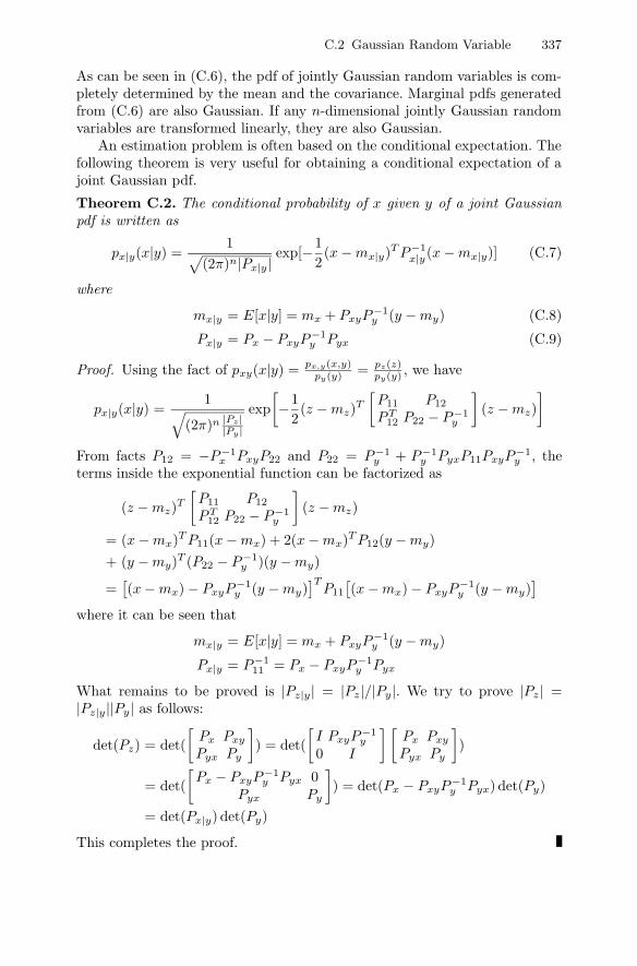
C.2 Gaussian Random Variable 337

As can be seen in (C.6), the pdf of jointly Gaussian random variables is com-pletely determined by the mean and the covariance. Marginal pdfs generatedfrom (C.6) are also Gaussian. If any n-dimensional jointly Gaussian randomvariables are transformed linearly, they are also Gaussian.

An estimation problem is often based on the conditional expectation. Thefollowing theorem is very useful for obtaining a conditional expectation of ajoint Gaussian pdf.

Theorem C.2. The conditional probability of x given y of a joint Gaussianpdf is written as

px|y(x|y) =1√

(2π)n|Px|y|exp[−1

2(x − mx|y)T P−1

x|y(x − mx|y)] (C.7)

where

mx|y = E[x|y] = mx + PxyP−1y (y − my) (C.8)

Px|y = Px − PxyP−1y Pyx (C.9)

Proof. Using the fact of pxy(x|y) = px,y(x,y)py(y) = pz(z)

py(y) , we have

px|y(x|y) =1√

(2π)n |Pz||Py|

exp[−1

2(z − mz)T

[P11 P12

PT12 P22 − P−1

y

](z − mz)

]

From facts P12 = −P−1x PxyP22 and P22 = P−1

y + P−1y PyxP11PxyP−1

y , theterms inside the exponential function can be factorized as

(z − mz)T

[P11 P12

PT12 P22 − P−1

y

](z − mz)

= (x − mx)T P11(x − mx) + 2(x − mx)T P12(y − my)+ (y − my)T (P22 − P−1

y )(y − my)

=[(x − mx) − PxyP−1

y (y − my)]T

P11

[(x − mx) − PxyP−1

y (y − my)]

where it can be seen that

mx|y = E[x|y] = mx + PxyP−1y (y − my)

Px|y = P−111 = Px − PxyP−1

y Pyx

What remains to be proved is |Pz|y| = |Pz|/|Py|. We try to prove |Pz| =|Pz|y||Py| as follows:

det(Pz) = det([

Px Pxy

Pyx Py

]) = det(

[I PxyP−1

y

0 I

] [Px Pxy

Pyx Py

])

= det([

Px − PxyP−1y Pyx 0

Pyx Py

]) = det(Px − PxyP−1

y Pyx) det(Py)

= det(Px|y) det(Py)

This completes the proof.

338 C Random Variables

Note that uncorrelatedness implies independence in the case of Gaussianrandom variables.

Theorem C.3. Let x, y, and z be joint Gaussian random variables. If y andz are independent, then E(x|y, z) = E(x|y) + E(x|z)−mx holds. For generalrandom variables y and z, the relation

E(x|y, z) = E(x|y, z) = E(x|y) + E(x|z) − mx

holds, where z = z − E(z|y).

Proof. In the case that y and z are independent, augmenting y and z into onevector ξ =

[yT zT

]T yields

E(x|y, z) = E(x|ξ) = mx + PxξP−1ξ (ξ − mξ)

Pxξ = E(xξT ) =[Pxy Pxz

]Pξ =

[Py 00 Pz

]from which we have

E(x|ξ) = mx + PxyP−1y (y − my) + PxzP

−1z (z − mz)

= E(x|y) + E(x|z) − mx

Now we consider the case that y and z are general, i.e. the independence oftwo random variables is not required. From Theorem C.2, z can be written as

z = z − Ez|y = z − mz − PzyP−1y (y − my) (C.10)

which means that x, y and z are jointly Gaussian. The mean of z, i.e. mz, is

mz = Ez − Ez|y = Ez − EEz|y = 0 (C.11)

It can be seen that y and z are uncorrelated as follows:

E(y − my)(z − mz)T = E(y − my)zT = EyzT = EyzT − EyEzT |y,= EyzT − EyzT = 0

It follows then that E(x|y, z) is written as

E(x|y, z) = mx + PxyP−1y (y − my) + PxzP

−1z z (C.12)

= E(x|y) + E(x|z) − mx

where

Pxz = Pxz − PxyP−1y Pyz

Pz = Pz − PzyP−1y Pyz

Through a trivial and tedious calculation for C.12, we obtain

E(x|y, z) = E(x|y, z)

This completes the proof.

C.3 Random Process 339

C.3 Random Process

Lemma C.4. Suppose that ui ∈ m is the wide sense stationary (WSS) inputsignal with power spectral density U(ejw) and yi ∈ p is the output signalcoming through the system H(ejw). The power of the output signal can berepresented as

E[yTi yi] = tr(E[yiy

Ti ]) =

12π

∫ 2π

0

tr(H(ejω)U(ejω)H∗(ejω)) dω (C.13)

It is noted that

E

[lim

N→∞1N

i0+N∑i=i0

yTi yi

]= E[yT

i yi] (C.14)

D

Linear Matrix Inequalities and SemidefiniteProgramming

D.1 Linear Matrix Inequalities

Now, we give a brief introduction to LMIs. The basic results of this appendixare from [BLEGB94].

We call F (x) an LMI if it has the following form:

F (x) = F0 +m∑

i=1

xiFi > 0 (D.1)

where the variable x = [x1 · · · xm]T ∈ Rm and the symmetric matricesFi = FT

i ∈ Rn×n, 0, · · · ,m are given. The inequality in (D.1) means thatF (x) is positive definite. It is noted that F (x) depends affinely on x.

The LMI (D.1) is convex on x, i.e. the set x|F (x) > 0 is convex. Eventhough the LMI (D.1) may seem to have a specialized form, it can representseveral nonlinear matrix inequalities, such as quadratic inequalities, includingRiccati inequalities, matrix norm inequalities, and constraints that arise incontrol theory.

Multiple LMIs F 1(x) > 0, · · · , F p(x) > 0 can be expressed as the followingsingle LMI:

diag(F 1(x), · · · , F p(x)) > 0

Therefore, it is usual to make no distinction between a set of LMIs and asingle LMI, i.e. “the LMIs F 1(x) > 0, · · · , F p(x) > 0” also means “the LMIdiag(F 1(x), · · · , F p(x)) > 0”.

Nonlinear matrix inequalities can be represented as LMIs, which is possibleusing the Schur complement. Consider the following LMI:[

Q(x) S(x)S(x)T R(x)

]> 0 (D.2)

where Q(x) and R(x) are symmetric. Note that Q(x), R(x), and S(x) dependaffinely on x. This LMI is equivalent to the following matrix inequalities:

342 D Linear Matrix Inequalities and Semidefinite Programming

R(x) > 0, Q(x) − S(x)R(x)−1ST (x) > 0 (D.3)

or equivalently:

Q(x) > 0, R(x) − ST (x)Q(x)−1S(x) > 0 (D.4)

The above equivalences can be easily proved by using the following matrixdecomposition:[

Q SST R

]=[

I 0ST Q−1 I

] [Q 00 R − ST Q−1S

] [I Q−1S0 I

]=[

I SR−1

0 I

] [Q − SR−1ST 0

0 R

] [I 0

R−1ST I

](D.5)

In other words, the set of nonlinear inequalities (D.3) or (D.4) can be repre-sented as the LMI (D.2). If R(x) and Q(x) are set to unit matrices, we havethe useful formula

I − SST > 0 ⇐⇒ I − ST S > 0 (D.6)

If R(x) and S(x) are set to a unit matrix and a vector x, we have

xxT < Q ⇐⇒ xT Q−1x < I (D.7)

where Q is assumed to be nonsingular.The matrix norm constraint ||Z(x)||2 < 1, where Z(x) ∈ Rp×q and de-

pends affinely on x, is represented as the LMI[I Z(x)

Z(x)T I

]> 0 (D.8)

from the fact that λmax(Z(x)T Z(x)) < 1 implies yT Z(x)T Z(x)y − yT y < 0for all y, i.e. Z(x)T Z(x) < I.

The constraint c(x)T P (x)−1c(x) < 1, P (x) > 0, where c(x) ∈ Rn andP (x) = P (x)T ∈ Rn×n depend affinely on x, is expressed as the LMI[

P (x) c(x)c(x)T 1

]> 0 (D.9)

More generally, the constraint

tr(S(x)T P (x)−1S(x)) < 1, P (x) > 0 (D.10)

where P (x) = P (x)T ∈ Rn×n depend affinely on x, is handled by introducinga new matrix variable X = XT ∈ Rp×p, and the LMI (in x and X)

tr(X) < 1,[

X S(x)T

S(x) P (x)

]> 0 (D.11)

D.2 Semidefinite Programming 343

Even though the variable x is given by a vector in the LMI (D.1), ma-trix variables can be used. Consider the following continuous version of theLyapunov inequality

AT P + PA < 0 (D.12)

where A ∈ Rn×n is given and P = P ′ is the variable which should be found.In this case, instead of representing the LMI explicitly in the form F (x) > 0,we will refer to (D.12) as the LMI where the matrix P is the variable. Ofcourse, the Lyapunov inequality (D.12) can be expressed as the form (D.1) byletting P1, · · · , Pm be a basis for symmetric n×n matrices and taking F0 = 0and Fi = −AT Pi − PiA.

As another example, consider the algebraic Riccati inequality

AT P + PA + PBR−1BT P + Q < 0, R > 0 (D.13)

where A, B, Q = QT , R = RT are given matrices of appropriate size, andP = PT is the variable. Inequality (D.13) can be expressed as the LMI[

AT P + PA + Q PBBT P −R

]< 0 (D.14)

We are often interested in whether a solution exists or not in an LMI.

• Feasibility problemsGiven LMI F (x) > 0, find a feasible solution xfeas such that F (xfeas) > 0or prove that a solution does not exist.

D.2 Semidefinite Programming

Now, we give a brief introduction to SDP which can effectively solve manyother optimization problems involving LMIs. The basic results are from[BLEGB94, VB96].

SDP is an optimization problem of minimizing a linear function of a vari-able x ∈ Rm subject to a matrix inequality:

minimize cT xsubject to F (x) > 0 (D.15)

where

F (x) = F0 +m∑

i=1

xiFi

This SDP is a convex optimization problem, since its objective and constraintare convex: if F (x) > 0 and F (y) > 0, then, for all λ, 0 ≤ λ ≤ 1,

344 D Linear Matrix Inequalities and Semidefinite Programming

F (λx + (1 − λy)) ≤ λF (x) + (1 − λy)F (y)

Even though the SDP (D.15) may seem to be quite specialized, it can rep-resent many important optimization problems, such as a linear programming(LP),

minimize cT xsubject to Gx < h

Gx < h ⇐⇒ diag(h1 h2 · · · hn) −n∑

i=1

xi diag(g1,i g2,i · · · gn,i) ≥ 0

a matrix norm minimization,

‖A‖22 < t2 ⇐⇒ λmax(AT A) < tI ⇐⇒ AT A < tI

⇐⇒ min t subject to[

tI AAT I

]> 0

a maximum eigenvalue minimization,

minimize λsubject to λI − A(x) > 0 (D.16)

where A is symmetric, and a quadratic programming (QP)

minimize 12xT Px + qT x + r

subject to Gx < h⇐⇒

minimize t

subject to[

t − r − qT x xT

x 2P−1

]> 0

Gx < h

Note that the quadratic programming problem involves minimization of aquadratic function subject to linear constraints.

In particular, it can represent a quadratic constrained QP (QCQP), whichis needed to solve the optimization problems. Now we will show how QCQPcan be cast as a special case of SDP. The convex quadratic constraint (Ax +b)T (Ax + b) − cT x − d < 0 can be expressed as[

I Ax + b(Ax + b)T cT x + d

]< 0

The left-hand side depends affinely on the vector x, and it can be also ex-pressed as

F (x) = F0 +m∑

i=1

xiFi

with

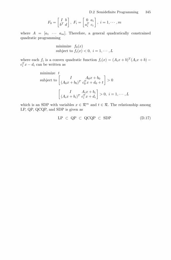
D.2 Semidefinite Programming 345

F0 =[

I bbT d

], Fi =

[0 ai

aTi ci

], i = 1, · · · ,m

where A = [a1 · · · am]. Therefore, a general quadratically constrainedquadratic programming

minimize f0(x)subject to fi(x) < 0, i = 1, · · · , L

where each fi is a convex quadratic function fi(x) = (Aix + b)T (Aix + b) −cTi x − di can be written as

minimize t

subject to[

I A0x + b0

(A0x + b0)T cT0 x + d0 + t

]> 0

[I Aix + bi

(Aix + bi)T cTi x + di

]> 0, i = 1, · · · , L

which is an SDP with variables x ∈ Rm and t ∈ R. The relationship amongLP, QP, QCQP, and SDP is given as

LP ⊂ QP ⊂ QCQP ⊂ SDP (D.17)

E

Survey on Applications

There are many papers that deal with applications of receding horizon con-trols. The terminology “MPC” is more popular in applications, so that we useit instead of “RHC”.

Most survey papers [RRTP78, GPM89, RMM94, Kwo94, May95, LC97,May97, CA98, ML99, MRRS00, KHA04] and books [BGW90, Soe92, Mos95,MSR96, AZ00, KC00, Mac02, Ros03, HKH02, CB04] also report real applica-tions of the RHC. There are a few survey papers on applications of industrialMPC technologies, particularly for process controls [OOH95] [QB97] [QB00][QB03].

We can consider two different kinds of applications. One is a softwareproduct for general uses and the other is a specific process where RHCs areapplied.

There are many commercial software products, such as Aspen Technol-ogy’s DMCPlus (Dynamic Matrix Control) and SMCA (Setpoint Multivari-able Contr. Arch.), Adersa’s IDCOM (identification and command), HIECON(Hierarchical Constraint Control), and PFC (Predictive Functional Control),Honeywell’s Profit Control, RMPCT (Robust MPC Technology), and PCT(Predictive Control Technology), Pavilion Technology’s Process Perfector,SCAP Europa’s APCS (Adaptive Predictive Control System), IPCOS’s INCA(IPCOS Novel Control Architecture), Simulation Sciences’ Connoisseur, andABB’s 3dMPC. This list may not be complete. For additional information,refer to [Mac02] [QB97][QB03].

Applied processes include refining, petrochemicals, chemicals, pulp andpaper, air and gas, utility, mining/metallurgy, food processing, polymer, fur-nace, aerospace/defence, automotive, ammonia synthesis, and so on. It is notso easy to list all applied processes. The surveys on the applied processescan be done by vendors [QB03] and manufacturers [OOH95]. In particular,applications of MPC are widely used in refining and petrochemical processes[QB03].

In the beginning, linear RHCs were applied. Recent years have shown rapidprogress in the development and application of industrial nonlinear MPC.

348 E Survey on Applications

When the operating points change frequently and span a sufficiently widerange of nonlinear process dynamics, the nonlinear MPC is very efficient com-pared with linear MPC. While applications of linear MPC are concentratedin refining, those of nonlinear MPC cover a much broader range of chem-icals, such as pH control, polymer manufacturing, and ammonia synthesis.However, it has been observed that the size of nonlinear MPC applications istypically much smaller than that of linear MPC [MJ98]. This is due to thecomputational complexity of nonlinear MPC.

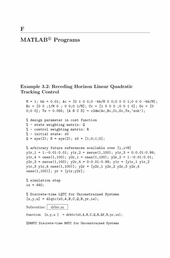
F

MATLAB Programs

Example 3.2: Receding Horizon Linear QuadraticTracking Control

M = 1; bb = 0.01; Ac = [0 1 0 0;0 -bb/M 0 0;0 0 0 1;0 0 0 -bb/M];Bc = [0 0 ;1/M 0 ; 0 0;0 1/M]; Cc = [1 0 0 0 ;0 0 1 0]; Dc = [00;0 0]; Ts = 0.055; [A B C D] = c2dm(Ac,Bc,Cc,Dc,Ts,’zoh’);

% design parameter in cost function% - state weighting matrix: Q% - control weighting matrix: R% - initial state: x0Q = eye(2); R = eye(2); x0 = [1;0;1;0];

% arbitrary future references available over [i,i+N]y1r_1 = 1:-0.01:0.01; y1r_2 = zeros(1,100); y1r_3 = 0:0.01:0.99;y1r_4 = ones(1,100); y2r_1 = ones(1,100); y2r_2 = 1:-0.01:0.01;y2r_3 = zeros(1,100); y2r_4 = 0:0.01:0.99; y1r = [y1r_1 y1r_2y1r_3 y1r_4 ones(1,100)]; y2r = [y2r_1 y2r_2 y2r_3 y2r_4ones(1,100)]; yr = [y1r;y2r];

% simulation stepis = 440;

% Discrete-time LQTC for Unconstrained Systems[x,y,u] = dlqtc(x0,A,B,C,Q,R,yr,is);

Subroutine: drhtc.m

function [x,y,u ] = drhtc(x0,A,B,C,Q,R,Qf,N,yr,is);

%DRHTC Discrete-time RHTC for Unconstrained Systems

350 F MATLAB Programs

% convert reference vector to row vector

[s1,s2] = size(yr); if (s2 == 1)

yr = yr’;

end

% check future reference length for simulation

if (length(yr) < (is + N))

disp(’The future reference is of too small length’);

return

end

% Riccati solution K(N-1) for RHTC

[K_N_1 K_history_vec] = drde2(A,B,C,Q,R,Qf,N);

% initialization of history variables

xi = x0; % state of plant x(i)

ui_history = []; % history of rhc u(i)

xi_history = x0; % history of state of plant x(i)

yi_history = C*x0; % history of output of plant y(i)

for i=1:is

% time-varying feed feedward gain g for RHTC

[g_1 g_history] = dvde(A,B,C,Q,R,Qf,N,K_history_vec,yr,i);

% receding horizon tracking controller u(i)

ui = -inv(R+B’*K_N_1*B)*B’*(K_N_1*A*xi+g_1);

% plant is controlled by rhtc u(i) at time [i,i+1]

xi = A*xi + B*ui;

yi = C*xi;

% history u(i), x(i), y(i)

ui_history = [ui_history ui];

xi_history = [xi_history xi];

yi_history = [yi_history yi];

end

x = xi_history; % state trajectory x

y = yi_history; % output trajectory y

u = ui_history; % RHTC history vector u

return

Subroutine: drde2.m

function [K_N_1,K_history_vec] = drde2(A,B,C,Q,R,Qf,N);

%DRDE2 Discrete-time Riccati Difference Equation Solver

F MATLAB Programs 351

% This RDE appears in LQ Tracking Problem

% system dimension

n = size(A,1);

% boundary condition

K_0 = C’*Qf*C; K_0_vec = mtx2vec(K_0); K_history_vec = K_0_vec;

K_i = K_0;

% solve Riccati Differential Equation 2

for i=1:N-1

K_i = A’*K_i*inv(eye(n)+B*inv(R)*B’*K_i)*A + C’*Q*C;

K_i_vec = mtx2vec(K_i);

K_history_vec = [K_history_vec K_i_vec];

end

% constant feedback gain K(N-1) for RHTC

[s1,s2] = size(K_history_vec); K_N_1 =

vec2mtx(K_history_vec(:,s2));

return

Subroutine: dvde.m

function [g_1,g_history ] =

dvde(A,B,C,R,Q,Qf,N,K_history_vec,yr,i );

%DVDE Discrete-time Vector Differential Equation Solver

% system dimension

n = size(A,1);

% boundary condition

g_N = -C’*Qf*yr(:,i+N); g_history = g_N; g_j = g_N;

% solve Vector Difference Equation

for j=(N-1):-1:1

K_j = vec2mtx(K_history_vec(:,(N-1)-j+1));

g_j = A’*inv(eye(n)+K_j*B*inv(R)*B’)*g_j - C’*Q*yr(:,i+j);

g_history = [g_history g_j];

end

% time-varying feed-forward gain g(1) for RHTC

[m,n] = size(g_history); g_1 = g_history(:,n);

return;

352 F MATLAB Programs

Example 3.3: Receding Horizon H∞ Tracking Control

clear;

% state-space model of original system and its discretization

M = 1; bb = 0.01; Ac = [0 1 0 0;0 -bb/M 0 0;0 0 0 1;0 0 0 -bb/M];

Bc = [0 0 ;1/M 0 ; 0 0;0 1/M]; Cc = [1 0 0 0 ;0 0 1 0]; Dc = [0

0;0 0]; Ts = 0.055;

[A B C D] = c2dm(Ac,Bc,Cc,Dc,Ts,’zoh’); Bw = [ 0 0 ; 0 0.03 ;

0.02 0 ; 0 0.05]

% design parameter in cost function

% - state weighting matrix: Q

% - control weighting matrix: R

% - disturbance weighting matrix: Rw

% - terminal weighting matrix: Qf

% - prediction horizon: N

system_order = size ( A , 1) ; input_order = size ( B , 2 ) ;

dist_order = size ( Bw , 2 ) ;

Q = eye(system_order) ; R = eye(input_order) ; Rw = 1.2

*eye(dist_order) ; N = 5 ; gamma_2 = 5.0 ;

% arbitrary future references available over [i,i+N]

y1r_1 = 1:-0.01:0.01; y1r_2 = zeros(1,100); y1r_3 = 0:0.01:0.99;

y1r_4 = ones(1,100); y2r_1 = ones(1,100); y2r_2 = 1:-0.01:0.01;

y2r_3 = zeros(1,100); y2r_4 = 0:0.01:0.99; y1r = [y1r_1 y1r_2

y1r_3 y1r_4 ones(1,100)]; y2r = [y2r_1 y2r_2 y2r_3 y2r_4

ones(1,100)]; yr = [y1r;y2r];

% simulation step

is = 440;

% Discrete-time RHTC for Unconstrained Systems

% initial state

x0 = [ 1 ; 0 ; 1 ; 0 ]; Qf = 100*eye(2); Q = eye(2) ;

gamma_2=1.5; Bw = [ 0.016 0.002 ; 0.01 0.009 ; 0.008 0 ; 0

0.0005] ;

[x_hinf,y_hinf,u_hinf , w] = drhtc_hinf ( x0 , A , B , Bw , C , Q

, R , Rw , Qf , gamma_2 , N , yr , is);

[x,y,u] = drhtc(x0,A,B,C,Q,R,Qf,N,yr,is, Bw,w);

F MATLAB Programs 353

for k = 0: is

y_rhtc_ws ( k+1 ,: ) = [ k*0.01 y(:,k+1)’ ];

end

for k = 0: is

r_rhtc_ws ( k+1 ,: ) = [k*0.01 yr(:,k+1)’];

end

for k = 0: is

y_rhtc_ws_hinf ( k+1 ,: ) = [k*0.01 y_hinf(:,k+1)’];

end

plot( r_rhtc_ws(:,2) , r_rhtc_ws(:,3) , y_rhtc_ws(:,2) ,

y_rhtc_ws(:,3) ,’-.’ , y_rhtc_ws_hinf(:,2) , y_rhtc_ws_hinf(:,3)

);

legend(’ Reference’,’H infinity RHTC’ , ’LQ RHTC’) ;

Subroutine: drhtc−hinf.m

function [ x , y , u , w] = drhtc_hinf ( x0 , A , B , Bw , C , Q

, R , Rw , Qf , gamma_2, N , yr , is);

% convert reference vector to row vector

[s1,s2] = size(yr); if (s2 == 1)

yr = yr’;

end

% check future reference length for simulation

if (length(yr) < (is + N))

disp(’The future reference is of too small length’);

return

end

% Riccati solution K(N-1) for RHTC

[K_N_1 K_history_vec] = drde2_hinf( A , B , Bw , C , Q , R , Rw ,

Qf , gamma_2 , N);

% initialization of history variables

xi = x0; % state of plant x(i)

ui_history = []; % history of rhc u(i)

xi_history = x0; % history of state of plant x(i)

yi_history = C*x0; % history of output of plant y(i)

wi_history = [];

system_order = size(A,1);

354 F MATLAB Programs

for i=1:is

% time-varying feed feedward gain g for RHTC

[g_1 g_history] = dvde_hinf( A , B , Bw , C , Q , R , Rw , Qf ,...

gamma_2, N , K_history_vec , yr , i);

% receding horizon tracking controller u(i)

Lambda = eye(system_order) + K_N_1 * ( B*inv(R)*B’ ...

- 1 / gamma_2 * Bw*inv(Rw)*Bw’) ;

ui = -inv(R) * B’ * inv( Lambda )*( K_N_1 * A * xi + g_1 ) ;

wi = 1/gamma_2* inv(Rw) * Bw’ * inv ( Lambda ) ...

* ( K_N_1 * A * xi + g_1 ) ;

% plant is controlled by rhtc u(i) at time [i,i+1]

xi = A*xi + B*ui + Bw*wi;

yi = C*xi;

ui_history = [ui_history ui];

xi_history = [xi_history xi];

yi_history = [yi_history yi];

wi_history = [wi_history wi];

end

x = xi_history; % state trajectory x

y = yi_history; % output trajectory y

u = ui_history; % RHTC history vector u

w = wi_history; % RHTC history vector u

return

Subroutine: drde2−hinf.m

function [K_N_1,K_history_vec] = drde2_hinf (A , B , Bw , C , Q

, R , Rw , Qf , gamma_2 , N );

% system dimension

n = size(A,1);

% boundary condition

K_0 = C’*Qf*C;

K_0_vec = mtx2vec(K_0); K_history_vec = K_0_vec; K_i = K_0;

% solve Riccati Differential Equation

F MATLAB Programs 355

for i=1:N-1

if min ( real ( eig ( Rw - 1 / gamma_2 *Bw’ * K_i * Bw) ) ) < 0

error (’error’);

end

Lambda = eye(n) + K_i * ( B*inv(R)*B’ - 1 / gamma_2 ...

* Bw * Rw^(-1) * Bw’ ) ;

K_i = A’ * inv(Lambda) * K_i *A + C’*Q*C;

K_i_vec = mtx2vec(K_i);

K_history_vec = [K_history_vec K_i_vec];

end

% constant feedback gain K(N-1) for RHTC

[s1,s2] = size(K_history_vec); K_N_1 =

vec2mtx(K_history_vec(:,s2)); return

Subroutine: dvde−hinf.m

function [g_1,g_history ] = dvde_hinf( A , B , Bw , C , Q , R ,

Rw , Qf , gamma_2, N , K_history_vec , yr , i);

n = size(A,1);

g_N = -C’*Qf*yr(:,i+N); g_history = g_N; g_j = g_N;

for j = (N-1): -1: 1

K_j = vec2mtx(K_history_vec(:,(N-1)-j+1));

Lambda = eye(n) + K_j * ( B*inv(R)*B’ ...

- 1/gamma_2 * Bw * inv(Rw) * Bw’ ) ;

%g_j = A’*inv(eye(n)+K_j*B*inv(R)*B’)*g_j - C’*Q*yr(:,i+j);

if ( Rw -

g_j = A’*inv(Lambda)*g_j - C’*Q*yr(:,i+j);

g_history = [g_history g_j];

end

% time-varying feed-forward gain g(1) for RHTC

[m,n] = size(g_history); g_1 = g_history(:,n); return;

Example 3.4: Cost Monotonicity Condition for RecedingHorizon Control

A = [ 0.6831 0.0353 ; 0.0928 0.6124 ] ; B = [0.6085;0.0158];

Q =eye(2); R =3;

356 F MATLAB Programs

SystemDim = size(A,1); InputDim = size(B,2);

% Getting started LMISYS description

setlmis([]);

% Defining LMI variables

Y=lmivar(2,[InputDim SystemDim]); X=lmivar(1,[SystemDim 1]);

% Defining LMI

lmiterm([-2 1 1 X],1,1); % LMI (1,1): X

lmiterm([-2 2 1 Y],B,1); % LMI (2,1): B*Y

lmiterm([-2 2 1 X],A,1); % LMI (2,1): A*X

lmiterm([-2 2 2 X],1,1); % LMI (2,2): X

lmiterm([-2 3 1 X],sqrt(Q),1); % LMI (3,1): Q^(1/2)*X

lmiterm([-2 3 3 0],1); % LMI (3,3): 1

lmiterm([-2 4 1 Y],sqrt(R),1); % LMI (4,1): R^(1/2)*Y

lmiterm([-2 4 4 0],1); % LMI (4,4): 1

LMISYS = getlmis; [tmin,xfeas]=feasp(LMISYS);

X=dec2mat(LMISYS,xfeas,X);

Example 4.1: Robustness of Minimum Variance FiniteImpulse Response filters

% Systems and paramteres %

A = [ 0.9305 0 0.1107; 0.0077 0.9802 -0.0173; 0.0142 0 0.8953];

B = [0.0217 0.2510; 0.0192 -0.0051; 0.0247 0.0030];

C = [ 1 0 0;0 1 0 ]; G = [1 1 1]’; Q = 0.02^2; R = 0.04^2*eye(2);

D_1 = 0; D_2 = 0;

N_sample = 250 ; N_order = size(A,1); N_horizon = 10;

% Making big matrices for FIR filters

[B_bar, C_bar, G_bar, Xi] = MakeBigMatrices (A,B,C,G,Q,R,10);

H = inv(C_bar’*inv(Xi) * C_bar) * C_bar’*inv(Xi);

% Parameter initialize

intial_state= [0 0 0 ]’; x = intial_state;

IIR_x_hat = [0 0 0]’; FIR_x_hat = IIR_x_hat;

P = 0.0*eye(N_order); real_state = zeros(N_order , N_sample);

estimated_state = zeros(N_order, N_sample); real_state(:,1)=x;

estimated_state(:,1) = IIR_x_hat;

FIR_estimated_state = zeros(N_order, N_sample);

measurements = zeros(2*N_sample);

F MATLAB Programs 357

delta_A = 0.1*[1 0 0;0 1 0;0 0 0.1 ];

delta_C = 0.1*[0.1 0 0;0 0.1 0 ];

% main procedure

for i = 1: N_sample-1

if( i > 50 & i < 101 )

x = (A+delta_A)*x + G*randn(1)*0.02;

y = (C+delta_C)*x + randn(2,1)*0.04;

else

x = A*x + G*randn(1)*0.02;

y = C*x + randn(2,1)*0.04;

end

real_state(:,i+1)=x;

% IIR_filter: one step predicted estimate

IIR_x_hat = A * IIR_x_hat + A * P *C’ * inv( R + C * P * C’)

*( y - C*IIR_x_hat);

P = A * inv( eye(N_order) + P * C’ * inv(R) * C) * P * A’

+ G * Q * G’;

estimated_state(:,i+1)=IIR_x_hat;

measurements(2*i-1:2*i) = y;

% FIR filter

if i>10

FIR_x_hat = H * (measurements(2*i-19:2*i))’;

end

FIR_estimated_state(:,i+1) = FIR_x_hat;

end

% Plot

plot( 1:N_sample , real_state(2,:)-estimated_state(2,:),

1:N_sample , real_state(2,:)-FIR_estimated_state(2,:))

Subroutine: MakeBigMatrices.m

function [B_bar , C_bar , G_bar , Xi] =

MakeBigMatrices(A,B,C,G,Q,R,horizon);

% Error check

A_inv = inv(A); IsInput = 1;

% initialization

358 F MATLAB Programs

if B == 0

IsInput = 0;

B_bar=0

else

B_bar = C * A_inv * B;

end

C_bar = C * A_inv; G_bar = -C * A_inv * G;

Q_stack = Q ; R_stack = R ; A_inv_i = A_inv;

% parameter setting

N_input = size(B,2); N_output = size(C,1);

N_system_noise = size(G,2); N_order = size(A,1);

% main procedure

for i = 2: horizon

A_inv_i = A_inv_i * A_inv ;

if IsInput == 1

B_bar = [B_bar -C_bar*A_inv*B; zeros(N_output, N_input*(i-1))

-C*A_inv*B ];

end

G_bar = [G_bar -C_bar*A_inv*G; zeros(N_output, N_system_noise*(i-1))

-C*A_inv*G ] ;

C_bar = [C * A_inv_i ;C_bar];

Q_stack = daug(Q_stack,Q); R_stack = daug(R_stack,R);

end

Xi = G_bar * Q_stack *G_bar’ + R_stack ;

Example 5.1: Linear Quadratic Finite Memory Control

% Systems and paramteres

A = [ 0.9305 0 0.1107; 0.0077 0.9802 -0.0173 ; 0.0142 0

0.8953 ]; B = [0.0217 0.2510 ;

0.0192 -0.0051 ;

0.0247 0.0030 ] ;

G = [1 1 1]’; C = [ 1 0 0;0 1 0 ]; Q = 0.02^2; R = 0.04^2*eye(2);

N=zeros(size(A,1),size(B,2));

D_1 = 0; D_2 = 0;

[K,S,E] = dlqr(A,B,eye(3),eye(2),N)

horizon_size =10;

F MATLAB Programs 359

% Making big matrices

[ B_bar , C_bar , G_bar , Xi] = MakeBigMatrices

(A,B,C,G,Q,R,horizon_size) ; H=inv(C_bar’*inv(Xi) * C_bar) *

C_bar’*inv(Xi);

N_sample = 800 ;

N_order = size(A,1); N_horizon = 10;

intial_state= [-1 1 1]’ ; x= intial_state ;

x_1=x; x_2=x;

IIR_x_hat = [0 0 0]’ ; FIR_x_hat = IIR_x_hat ;

P = 0.5*eye(N_order) ; real_state = zeros(N_order , N_sample);

IIR_state = zeros(N_order, N_sample); real_state(:,1)=x;

IIR_state(:,1)=IIR_x_hat; measurements = zeros ( 2*N_sample);

FIR_state = zeros(N_order, N_sample);

% Temporary uncertainty

delta_A = 0.05*[1 0 0;0 1 0;0 0 0.1 ]; delta_C = 0.05*[0.1 0 0;0

0.1 0 ];

% Start time and stop time of temporary uncertainty

dist_start = 300; dist_stop = 501;

for i = 1: N_sample-1

% FIR

sys_noise=randn(1)*0.01;

mea_noise=randn(2,1)*0.01;

if( i > dist_start & i < dist_stop )

x_1 = (A+delta_A)*x_1 - B*K*FIR_x_hat + G*sys_noise;

y_1 = (C+delta_C)*x_1 + mea_noise;

else

x_1 = A*x_1 - B*K*FIR_x_hat +G*sys_noise;

y_1 = C*x_1 + mea_noise;

end

FIR_state(:,i+1) = x_1;

measurements(2*i-1:2*i) = y_1;

if i>10

FIR_x_hat = H * (measurements(2*i-(2*horizon_size-1):2*i))’;

else

FIR_x_hat = zeros(N_order,1);

end

% IIR

if( i > dist_start & i < dist_stop )

x_2 = (A+delta_A)*x_2 - B*K*IIR_x_hat + G*sys_noise;

y_2 = (C+delta_C)*x_2 + mea_noise;

else

360 F MATLAB Programs

x_2 = A*x_2 - B*K*IIR_x_hat +G*sys_noise;

y_2 = C*x_2 + mea_noise;

end

IIR_state(:,i+1) = x_2;

IIR_x_hat = A * IIR_x_hat + A* P *C’ *

inv( R + C * P * C’)*( y_2 - C*IIR_x_hat);

P = A * inv( eye(N_order) + P * C’ * inv(R) * C) * P * A’ + G * Q * G’;

end

% plot

time = 1:N_sample; time = time*0.05;

plot( time ,-IIR_state(1,1:N_sample),’r’,time,-FIR_state(1,1:N_sample),’b’ );

title(’First state trajectory’); xlabel(’Time’); figure;

plot( time ,-IIR_state(2,1:N_sample),’r’ ,time ,-FIR_state(2,1:N_sample),’b’);

title(’Second state trajectory’); xlabel(’Time’); figure;

plot( time ,-IIR_state(3,1:N_sample),’r’ ,time,-FIR_state(3,1:N_sample),’b’ );

title(’Third state trajectory’); xlabel(’Time’);

Subroutine: MakeBigMatrices.m

function [B_bar , C_bar , G_bar , Xi ] =

MakeBigMatrices(A,B,C,G,Q,R,horizon);

A_inv = inv(A);

IsInput = 1;

% initialization

if B == 0

IsInput = 0;

B_bar=0

else

B_bar = C * A_inv * B;

end

C_bar = C * A_inv;

G_bar = -C * A_inv * G;

Q_stack = Q ;

R_stack = R ;

A_inv_i = A_inv

% parameter setting

N_input = size(B,2);

N_output = size(C,1);

N_system_noise = size(G,2);

N_order = size(A,1);

% main procedure

for i = 2: horizon

i

A_inv_i = A_inv_i * A_inv ;

if IsInput == 1

B_bar = [ B_bar -C_bar*A_inv*B ;

zeros(N_output , N_input*(i-1)) -C*A_inv*B ];

F MATLAB Programs 361

end

G_bar = [ G_bar -C_bar*A_inv*G ; zeros(N_output ,

N_system_noise*(i-1)) -C*A_inv*G ] ;

C_bar = [ C * A_inv_i ;C_bar];

Q_stack = daug(Q_stack,Q);

R_stack = daug(R_stack,R);

end

Xi = G_bar * Q_stack *G_bar’ + R_stack ;

Example 6.2: Constrained Receding Horizon Control

% Demonstration of RHC using LMI

clear all;

%% System State Equation

A= [1 0.2212;

0 0.7788];

B = [0.0288;0.2212]; G =[1 0; 0 1; 1.5 1];

%% Initial State

x0 = [1;0.3];

[n,n]=size(A); [n,m]=size(B);

% Let’s get predictor

N = input(’horizon N =’ ); length = input(’total simu time?=’);

% Input Constraint

u_lim=0.5; ubar_lim = []; for i=1:N,

ubar_lim=[ubar_lim;u_lim];

end

% State Constraint

x_lim = [1.5;0.3]; G =[1 0;

0 1];

g_lim = [1.5; 0.3]; gbar_lim = []; for i=1:N,

gbar_lim=[gbar_lim;g_lim];

end

[ng_r, ng_c] = size(G);

% Weighting Matrix

Q = 1*eye(size(A)); R = 1;

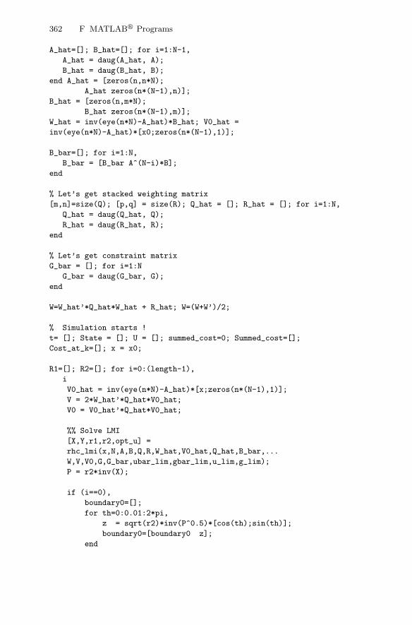
362 F MATLAB Programs

A_hat=[]; B_hat=[]; for i=1:N-1,

A_hat = daug(A_hat, A);

B_hat = daug(B_hat, B);

end A_hat = [zeros(n,n*N);

A_hat zeros(n*(N-1),n)];

B_hat = [zeros(n,m*N);

B_hat zeros(n*(N-1),m)];

W_hat = inv(eye(n*N)-A_hat)*B_hat; V0_hat =

inv(eye(n*N)-A_hat)*[x0;zeros(n*(N-1),1)];

B_bar=[]; for i=1:N,

B_bar = [B_bar A^(N-i)*B];

end

% Let’s get stacked weighting matrix

[m,n]=size(Q); [p,q] = size(R); Q_hat = []; R_hat = []; for i=1:N,

Q_hat = daug(Q_hat, Q);

R_hat = daug(R_hat, R);

end

% Let’s get constraint matrix

G_bar = []; for i=1:N

G_bar = daug(G_bar, G);

end

W=W_hat’*Q_hat*W_hat + R_hat; W=(W+W’)/2;

% Simulation starts !

t= []; State = []; U = []; summed_cost=0; Summed_cost=[];

Cost_at_k=[]; x = x0;

R1=[]; R2=[]; for i=0:(length-1),

i

V0_hat = inv(eye(n*N)-A_hat)*[x;zeros(n*(N-1),1)];

V = 2*W_hat’*Q_hat*V0_hat;

V0 = V0_hat’*Q_hat*V0_hat;

%% Solve LMI

[X,Y,r1,r2,opt_u] =

rhc_lmi(x,N,A,B,Q,R,W_hat,V0_hat,Q_hat,B_bar,...

W,V,V0,G,G_bar,ubar_lim,gbar_lim,u_lim,g_lim);

P = r2*inv(X);

if (i==0),

boundary0=[];

for th=0:0.01:2*pi,

z = sqrt(r2)*inv(P^0.5)*[cos(th);sin(th)];

boundary0=[boundary0 z];

end

F MATLAB Programs 363

elseif(i==1),

boundary1=[];

for th=0:0.01:2*pi,

z = sqrt(r2)*inv(P^0.5)*[cos(th);sin(th)];

boundary1=[boundary1 z];

end

elseif(i==2),

boundary2=[];

for th=0:0.01:2*pi,

z = sqrt(r2)*inv(P^0.5)*[cos(th);sin(th)];

boundary2=[boundary2 z];

end

elseif(i==3),

boundary3=[];

for th=0:0.01:2*pi,

z = sqrt(r2)*inv(P^0.5)*[cos(th);sin(th)];

boundary3=[boundary3 z];

end

elseif(i==4),

boundary4=[];

for th=0:0.01:2*pi,

z = sqrt(r2)*inv(P^0.5)*[cos(th);sin(th)];

boundary4=[boundary4 z];

end

end

K = Y*inv(X);

u = opt_u(1);

State = [State x];

U = [U u]; %% Control Input

cost_at_k = r1+r2;

real_cost = x’*Q*x + u’*R*u;

R1=[R1 r1];

R2=[R2 r2];

summed_cost = summed_cost + real_cost;

Cost_at_k = [Cost_at_k cost_at_k];

Summed_cost = [Summed_cost summed_cost];

% State Update

x = A*x + B*u;

t= [t i+1];

home;

end

Cost_at_k=[Cost_at_k Cost_at_k(length)]; Summed_cost=[Summed_cost

Summed_cost(length)]; U=[U u]; State=[State x]; t=[ 0 t];R2=[R2

R2(length)];R1=[R1 R1(length)];

364 F MATLAB Programs

% Let’s take a look at the simulation results

figure; plot(t,State(1,:),’r:’,t,State(2,:),’b’);

legend(’x1’,’x2’,0); xlabel(’time(sec)’);grid; title(’states’);

if (i>5), figure;

plot(State(1,:),State(2,:),’o’,boundary0(1,:),boundary0(2,:),’b’,

boundary1(1,:),boundary1(2,:),’r’,...

boundary2(1,:),boundary2(2,:),’k’,boundary3(1,:),boundary3(2,:),...

’r’,boundary4(1,:),boundary4(2,:),’r’); axis([-1.7 1.7 -0.35

0.35]);

end

figure; stairs(t,U); xlabel(’time(sec)’);grid; title(’control

input’);

figure; stairs(t,Cost_at_k,’r’); xlabel(’time(sec)’);grid;

title(’Expected cost at time k’);

figure; stairs(t,Summed_cost,’b’);grid; xlabel(’time(sec)’);

title(’Summed cost’);

figure; plot(t,R1,’r’,t,R2,’b’);

Subroutine: dvde−rhclmi.m

% Function: rhc_lmi.m

%

function [X_opt,Y_opt,r1_opt,r2_opt,u_opt] =

rhc_lmi(x,N,A,B,Q,R,W_hat,V0_hat,Q_hat,B_bar,W,V,V0,G,G_bar,...

ubar_lim,gbar_lim,u_lim,g_lim)

% LMI Variable = X, Y, r1, r2, U

[n,n]=size(A); [n,nu]=size(B); [nG_r, nG_c]= size(G); [nglim_r,

nglim_c]= size(g_lim);

if (~isempty(G_bar)),

GW = G_bar*W_hat;

gg1 = gbar_lim + G_bar*V0_hat;

gg2 = gbar_lim-G_bar*V0_hat;

end [nGW_r,nGW_c] = size(GW);

setlmis([]);

% LMI Variable

r1 = lmivar(1,[1 0]); r2 = lmivar(1,[1 0]); X = lmivar(1,[n 1]); Y

= lmivar(2,[nu n]); Z = lmivar(1,[nu 1]); U = lmivar(2,[N*nu 1]);

VV = lmivar(1,[nglim_r 1]);

F MATLAB Programs 365

lmiterm([-1 1 1 r1], 1, 1); lmiterm([-1 1 1 U], 0.5*V’,1,’s’);

lmiterm([-1 1 1 0], -V0); %% (1,1) = r1-V’*U -V0

lmiterm([-1 2 1 U], W^0.5, 1); %% (2,1) = W^0.5*U

lmiterm([-1 2 2 0], 1); %% (2,2) = I

lmiterm([-2 1 1 0],1); %% (1,1) = 1

lmiterm([-2 2 1 0],A^N*x); %% (2,1) = A^N*x

lmiterm([-2 2 1 U], B_bar,1); %% (2,1) = A^N*x + B_bar*U

lmiterm([-2 2 2 X],1,1); %% (2,2) = X

lmiterm([-3 1 1 X], 1, 1); %% (1,1) = X

lmiterm([-3 2 2 X], 1, 1); %% (2,2) = X

lmiterm([-3 3 3 r2], 1,1); %% (3,3) = r2*I

lmiterm([-3 4 4 r2], 1, 1); %% (4,4) = r2*I

lmiterm([-3 2 1 X], A, 1);

lmiterm([-3 2 1 Y], B, 1); %% (2,1) = A*X + B*Y

lmiterm([-3 3 1 X], real(Q^0.5), 1); %% (3,1) = Q^0.5*X

lmiterm([-3 4 1 Y], R^0.5, 1); %% (4,1) = R^0.5*X

% Constraint on u during the horizon from 0 to N-1

Ucon_LMI_1 = newlmi; for i=1:N*nu,

tmp = zeros(nu*N,1);

tmp(i,1) = 1;

%% U(i) >= -ubar_lim(i)

lmiterm([-(Ucon_LMI_1+i-1) 1 1 U], 0.5*tmp’,1,’s’);

lmiterm([-(Ucon_LMI_1+i-1) 1 1 0], ubar_lim(i));

%% U(i) <= ubar_lim(i)

lmiterm([(Ucon_LMI_1+N*nu+i-1) 1 1 U], 0.5*tmp’, 1,’s’);

lmiterm([(Ucon_LMI_1+N*nu+i-1) 1 1 0], -ubar_lim(i));

end

% Constraint on u after the horizon N

Ucon_LMI_2 = newlmi;

lmiterm([-Ucon_LMI_2 1 1 Z], 1,1); %% (1,1) = Z

lmiterm([-Ucon_LMI_2 1 2 Y], 1,1); %% (1,2) = Y

lmiterm([-Ucon_LMI_2 2 2 X], 1,1); %% (2,2) = X

Ucon_LMI_3 = newlmi; for i=1:nu,

tmp = zeros(nu,1);

tmp(i,1) = 1;

lmiterm([(Ucon_LMI_3+i-1) 1 1 Z], tmp’, tmp);

%% (1,1) Z(i,i) <= u_lim(i)^2

lmiterm([(Ucon_LMI_3+i-1) 1 1 0], -u_lim(i)^2);

end

% Constraint on x during the horizon from 0 to N-1

366 F MATLAB Programs

if (~isempty(G_bar)),

Xcon_LMI1 = newlmi;

for i=1:nGW_r,

%% (1,1) GW*U + gg1 > = 0

lmiterm([-(Xcon_LMI1+i-1) 1 1 U], 0.5*GW(i,:),1,’s’);

lmiterm([-(Xcon_LMI1+i-1) 1 1 0], gg1(i));

%% (1,1) -GW*U + gg2 >= 0

lmiterm([-(Xcon_LMI1+nGW_r+i-1) 1 1 U], -0.5*GW(i,:),1,’s’)

lmiterm([-(Xcon_LMI1+nGW_r+i-1) 1 1 0], gg2(i));

end

end

% Constraint on x after the horizon N

if (~isempty(G)),

X_con_LMI2 = newlmi;

lmiterm([X_con_LMI2 1 1 X], G, G’);

lmiterm([X_con_LMI2 1 1 VV], -1, 1); %% (1,1) G*X*G’ <= VV

for i=1:nglim_r,

tmp = zeros(nglim_r,1);

tmp(i,1) = 1;

lmiterm([(X_con_LMI2+i) 1 1 VV], tmp’,tmp);

%% (1,1) VV(i,i) <= g_lim(i)^2

lmiterm([(X_con_LMI2+i) 1 1 0], -g_lim(i)^2);

end

end

rhclmi = getlmis;

% Now we’re ready to solve LMI

n_lmi = decnbr(rhclmi); c = zeros(n_lmi,1); for j=1:n_lmi,

[r1j, r2j]= defcx(rhclmi,j,r1,r2);

c(j) = r1j + r2j;

end

[copt, Uopt]= mincx(rhclmi, c’, [1e-6 300 0 0 0]);

u_opt = dec2mat(rhclmi, Uopt, U); r1_opt = dec2mat(rhclmi, Uopt,

r1); r2_opt = dec2mat(rhclmi, Uopt, r2); X_opt = dec2mat(rhclmi,

Uopt, X); Y_opt = dec2mat(rhclmi, Uopt, Y);

References

[AHK04] C. K. Ahn, S. Han, and W. H. Kwon. Minimax finite memory controlsfor discrete-time state-space systems. Seoul Nat’l Univ., School of EE& CS Tech. Report No. SNU-EE-TR-2004-3, 2004-3, Nov. 2004.

[AM80] B. D. O. Anderson and J. B. Moore. Coping with singular transition ma-trices in estimation and control stability theory. Int. J. Contr., 31:571–586, 1980.

[AM89] D. O. Anderson and J. B. Moore. Optimal Control: Linear QuadraticMethods. Prentice-Hall International Editions, Englewood Cliffs, NJ07632, 1989.

[Ath71] M. A. Athans. Special issue on the LQG problem. IEEE Trans. Au-tomat. Contr., 16(6):527–869, 1971.

[AW73] K. J. Astrom and B. Wittenmark. On self-tuning regulators. Automat-ica, 9(2):185–199, 1973.

[AZ99] F. Allgower and A. Zheng. Nonlinear predictive control: assessmentand future directions. In Proc. of International Workshop on ModelPredictive Control, Ascona 1998, Springer, Berlin, 1999.

[AZ00] Frank Allgower and Alex Zhen. Nonlinear Model Predictive Control(Progress in Systems and Control Theory. Birkhauser,Boston, 2000.

[BB91] T. Basar and P. Bernhard. H∞ – Optimal Control and Related MinimaxDesign Problems: A Dynamic Game Approach. Birkhauser, Boston,1991.

[BD62] R. E. Bellman and S. E. Dreyfus. Applied Dynamic Programming.Princeton University Press, Princeton, NJ, 1962.

[Bel57] R. E. Bellman. Dynamic Programming. Princeton University Press,Princeton, NJ, 1957.

[BGFB94] S. Boyd, L. E. Ghaoui, E. Feron, and V. Balakrishnan. Linear MatrixInequalities in System and Control Theory, volume 15. SIAM, Philadel-phia, PA, 1994.

[BGP85] R. R. Bitmead, M. Gevers, and I. R. Petersen. Monotonicity and sta-bilizability properties of solutions of the Riccati difference equation:propositions, lemmas, theorems, fallacious conjecture and counterex-amples. Systems and Control Letters, 5:309–315, 1985.

[BGW90] R. R. Bitmead, M. Gevers, and V. Wertz. Adaptive Optimal Control:The Thinking Man’s GPC. Prentice-Hall, 1990.

368 References

[BH75] A. D. Bryson and Y. C. Ho. Applied Optimal Control. John Wiley &Sons, Inc., Hemisphere, New York, 1975.

[BH89] D. S. Berstein and W. Haddad. Steady-state kalman filtering with h∞error bound. Systems and Control Letters, 12:9–16, 1989.

[Bie75] G. J. Bierman. Fixed memory least squares filtering. IEEE Trans.Automat. Contr., 20:690–692, 1975.

[BK65] R. E. Bellman and R. E. Kalaba. Dynamic Programming and ModernControl Theory. Academic Press, New York, 1965.

[BK85] A. M. Bruckstein and T. Kailath. Recursive limited memory filteringand scattering theory. IEEE Trans. Inform. Theory, 31:440–443, 1985.

[Bla91] F. Blanchini. Constrained control for uncertain linear systems. Journalof Optimizaton Theory and Applications, pages 465–484, 1991.

[BLEGB94] S. Boyd, E. Feron L. E. Ghaoui, and V. Balakrishnan. Linear matrixinequalities in system and control theory. System and Control Theory,1994.

[BLW91] Sergio Bittanti, Alan J. Laub, and Jan C. Willems. The Riccati Equa-tion. Springer-Verlag, 1991.

[BO82] T. B. and G. J. Olsde. Dynamic Noncooperative Game Theory. Aca-demic Press, London, New York, 1982.

[Bur98] Jeffrey B. Burl. Linear Optimal Control. Addison-Wesley, California,1998.

[Bux74] P. J. Buxbaum. Fixed-memory recursive filters. IEEE Trans. Inform.Theory, 20:113–115, 1974.

[CA98] H. Chen and F. Allgower. Nonlinear model predictive control schemeswith guaranteed stabilty. In NATO ASI on Nonlinear Model BasedProcess Control, 465–494, 1998.

[CB04] E. F. Camacho and C. Bordons. Model Predictive Control (AdvancedTextbooks in Control and Signal Processing). Springer Verlag, 2004.

[CG79] D. W. Clarke and P. J. Gawthrop. Self-tuning control. IEE Proc. Pt.D, 126(6):633–640, 1979.

[Cla94] D. W. Clarke. Advances in model-based predictive control. Advancesin Model-Based Predictive Control, pages 2–21, 1994.

[CMT87] D. W. Clarke, C. Mohtadi, and P. S. Tuffs. Generalized predictivecontrol– part I. the basic algorithm. Automatica, 23(2):137–148, 1987.

[CR80] C. R. Cutler and B. L. Ramaker. Dynamic matrix control: a computercontrol algorithm. In Joint Automatic Control Conf., San Francisco,U.S.A, 1980.

[DC93] H. Demircioglu and D. W. Clarke. Generalised predictive control withend point weighting. IEE Proc. Pt. D, 140(4):275–282, 1993.

[DX94] Liu Danyang and Liu Xuanhuang. Optimal state estimation without therequirement of a priori statistics information of the initial state. IEEETrans. Automat. Contr., 39(10):2087–2091, 1994.

[EWMR94] R. W. Eustace, B. A. Woodyatt, G. L. Merrington, and A. Runacres.Fault signatures obtained from fault implant tests on an F404 engine.ASME Trans. J. of Engine, Gas Turbines, and Power, 116(1):178–183,1994.

[GL95] M. Green and D. J. N. Limebeer. Linear Robust Control. Prentice-Hall,Englewood Cliffs, New Jersey, 1995.

[GNLC95] P. Gahinet, A. Nemirovski, A. J. Laub, and M. Chilali. LMI ControlToolbox. The MATHWORKS Inc., USA, 1995.

References 369

[GPM89] C. E. Garcıa, D. M. Prett, and M. Morari. Model predictive control:Theory and practice–a survey. Automatica, 25(3):335–348, 1989.

[Gri02] M. J. Grimble. Workshop on nonlinear predictive control. Oxford Uni-versity, 18–19 July, 2002.

[GT91] Elmer G. Gilbert and Kok Tin Tan. Linear systems with state andcontrol constraints: the theory and application of maximal output ad-missible sets . IEEE Trans. on Auto. Control, 36(9):1008–1020, 1991.

[Gyu02] E. Gyurkovics. Receding horizon h∞ control for nonlinear discrete-timesystems. IEE Proc.-Control Theory Appl., 149(6):540–546, 2002.

[HK04] S. Han and W. H. Kwon. Receding horizon finite memory controls foroutput feedback controls of disrete-time state space models. In Proc. ofthe 30th Annual Conference of the IEEE Industrial Electronics Society,Busan, Korea, 2004.

[HKH02] Sunan Huang, Tan Kok Kiong, and Lee Tong Heng. Applied PredictiveControl. Springer Verlag, 2002.

[HKK99] S. Han, P. S. Kim, and W. H. Kwon. Receding horizon FIR filter withestimated horizon initial state and its application to aircraft enginesystems . In Proc. IEEE Int. Conf. Contr. Applications, pages 33–38,Hawaii, USA, 1999.

[HKK01] S. Han, W. H. Kwon, and Pyung Soo Kim. Receding horizon unbiasedFIR filters for continuous-time state space models without a priori initialstate information. IEEE Trans. Automat. Contr., 46(5):766–770, 2001.

[HKK02] S. Han, W. H. Kwon, and Pyung Soo Kim. Quasi-deadbeat minimax fil-ters for deterministic state-space models. IEEE Trans. Automat. Contr.,47(11):1904–1908, 2002.

[HSK99] Babak Hassibi, Ali H. Sayed, and Thomas Kailath. Indefinite QuadraticEstimation and Control. SIAM studies in applied and numerical math-ematics, 1999.

[Jaz68] A. H. Jazwinski. Limited memory optimal filtering. IEEE Trans. Au-tomat. Contr., 13:558–563, 1968.

[JHK04] J. W. Jun, S. Han, and W. H. Kwon. Fir filters and dual iir filters. SeoulNat’l Univ., School of EE & CS Tech. Report No. SNU-EE-TR-2004-6,2004-6, Nov. 2004.

[Kal63] R. E. Kalman. Lyapunov functions for the problem of lur’e in automaticcontrol. Proc. Nat. Acad. Sci., 49:201–205, 1963.

[KB60] R. E. Kalman and R. S. Bucy. A new approach to linear filtering andprediction problems. Trans. ASME J. of Basic Engr., 82:35–45, 1960.

[KB61] R. E. Kalman and R. S. Bucy. New results in linear filtering and pre-diction theory. Trans. ASME J. of Basic Engr., 83:95–108, 1961.

[KB89] W. H. Kwon and D. G. Byun. Receding horizon tracking control as apredictive control and its stability properties. Int. J. Contr., 50:1807–1824, 1989.

[KBK83] W. H. Kwon, A. M. Bruckstein, and T. Kailath. Stabilizing state-feedback design via the moving horizon method. Int. J. Contr., 37:631–643, 1983.

[KBM96] M. V. Kothare, V. Balakrishnan, and M. Morari. Robust constrainedmodel predictive control using linear matrix inequalities. Automatica,32:1361–1379, 1996.

[KC00] Basil Kourvaritakis and Mark Cannon. Nonlinear Predictive Control:Theory & Practice. IEE Publishing, 2000.

370 References

[KG88] S. S. Keerthi and E. G. Gilbert. Optimal infinite-horizon feedback lawsfor a general class of constrained discrete-time systems: stability andmoving-horizon approximation. J. of Optimization Theory and Appli-cations, 57:265–293, 1988.

[KG98] I. Kolmanovsky and E. C. Gilbert. Theory and computation of distur-bance invariant sets for discrete-time linear systems. Math. Prob. Eng.,pages 117–123, 1998.

[KGC97] J. C. Kantor, C. E. Garcia, and B. Carnahan. In In Fifth InternationalConference on Chemical Process Control, CACHE, A.I.Ch.E., 1997.

[KH04] W. H. Kwon and S. Han. Receding horizon finite memory controls foroutput feedback controls of state space models. IEEE Trans. Automat.Contr., 49(11):1905–1915, 2004.

[KHA04] W. H. Kwon, S. Han, and C. K. Ahn. Advances in nonlinear predictivecontrol: A survey on stability and optimality. International Journal ofControl, Automations, and Systems, 2(1):15–22, 2004.

[KIF93] Hans W. Knobloch, Alberto Isisori, and Dietrich Flockerzi. Topics inControl Theory. Birkhauser Verlag, 1993.

[Kir70] D. E. Kirk. Optimal Control Theory. Prentice-Hall, Englewood Cliffs,New Jersey, 1970.

[KK00] W. H. Kwon and K. B. Kim. On stabilizing receding horizon controlsfor linear continuous time-invariant systems. IEEE Trans. Automat.Contr., 45(7):1329–1334, 2000.

[KKH02] W. H. Kwon, Pyung Soo Kim, and S. Han. A receding horizon unbiasedFIR filter for discrete-time state space models. Automatica, 38(3):545–551, 2002.

[KKP99] W. H. Kwon, P. S. Kim, and P. Park. A receding horizon Kalman FIRfilter for discrete time-invariant systems. IEEE Trans. Automat. Contr.,44(9):1787–1791, 1999.

[Kle70] D. L. Kleinman. An easy way to stabilize a linear constant system.IEEE Trans. Automat. Contr., 15:692, 1970.

[Kle74] D. L. Kleinman. Stabilizing a discrete, constant, linear system withapplication to iterative methods for solving the Riccati equation. IEEETrans. Automat. Contr., 19:252–254, 1974.

[KP77a] W. H. Kwon and A. E. Pearson. A modified quadratic cost problemand feedback stabilization of a linear system. IEEE Trans. Automat.Contr., 22(5):838–842, 1977.

[KP77b] W. H. Kwon and A. E. Pearson. A note on the algebraic matrix Riccatiequation. IEEE Trans. on Automat. Contr., 22:143–144, 1977.

[KP77c] W. H. Kwon and A. E. Pearson. A modified quadratic cost problem andfeedback stabilization of a linear discrete time system. Brown Univ.,Div. Eng. Tech. Rep., AFOSR-75-2793C/1, Sept. 1977.

[KP78] W. H. Kwon and A. E. Pearson. On feedback stabilization oftime-varying discrete linear systems. IEEE Trans. Automat. Contr.,23(3):479–481, 1978.

[KRC92] B. Kouvaritakis, J. A. Rossiter, and A. O. T. Chang. Stable generalisedpredictive control: an algorithm with guaranteed stability. IEE Proc.Pt. D, 139(4):349–362, 1992.

[KS72] H. Kwakernaak and R. Sivan. Linear Optimal Control Systems. WileyInterscience, 1972.

References 371

[KSH00] Thomas Kailath, Ali H. Sayed, and Babak Hassibi. Linear Estimation.Prentice Hall, 2000.

[Kuc91] V. Kucera. Analysis and Design of Discrete Linear Control Systems.Prentice Hall, 1991.

[Kwo94] W. H. Kwon. Advances in predictive control: theory and application.In Asian Control Conference, Tokyo, 1994.

[KYK01] K. B. Kim, Tae-Woong Yoon, and W. H. Kwon. On stabilizing recedinghorizon H∞ controls for linear continuous time-varying systems. IEEETrans. Automat. Contr., 46(8):1273–1279, 2001.

[LAKG92] D. J. J. Limbeer, B. D. O. Anderson, P. P. Khargonekar, and M. Green.A game theoretic approach to H∞ control for time varing systems. SIAMJournal of Control and Optimization, 30(2):262–283, 1992.

[LC97] J. H. Lee and B. Cooley. Recent advances in model predictive controland other related areas. In Fifth International Conference on ChemicalProcess Control, CACHE, AIChE, pages 201–216, 1997.

[Lew86a] F. L. Lewis. Optimal Control. John Wiley & Sons, Inc., 1986.[Lew86b] F. L. Lewis. Optimal estimation. John Wiley & Sons, Inc., 1986.[LG94] S. Lall and K. Glover. A game theoretic approach to moving horizon

control. Advances in Model-Based Predictive Control, pages 131–144,1994.

[LHK04] Y. S. Lee, S. Han, and W. H. Kwon. Nonlinear receding horizon controlswith quadratic cost functions. Seoul Nat’l Univ., School of EE & CSTech. Report No. SNU-EE-TR-2004-7, 2004-7, Nov. 2004.

[LK99] Y. I. Lee and B. Kouvaritakis. Constrained receding horizon predictivecontrol for systems with disturbances. Int. J. Control, 72(11):1027–1032,1999.

[LK01] Y. I. Lee and B. Kouvaritakis. Receding horizon output feedback controlfor linear systems with input saturation. IEE Proc.-Control TheoryAppl., 148(2):109–115, 2001.

[LKC98] J. W. Lee, W. H. Kwon, and J. H. Choi. On stability of constrainedreceding horizon control with finite terminal weighting matrix. Auto-matica, 34(12):1607–1612, 1998.

[LKL99] J. W. Lee, W. H. Kwon, and J. H. Lee. Receding horizon H∞ trackingcontrol for time-varying discrete linear systems. Int. J. Contr., 68:385–399, 1999.

[LL99] K. V. Ling and K. W. Lim. Receding horizon recursive state estimation.IEEE Trans. Automat. Contr., 44(9):1750–1753, 1999.

[Mac02] J. M. Maciejowski. Predictive Control with Constraints. Prentice Hall,2002.

[May95] D. Q. Mayne. Optimization in model based control. In Proc. of the IFACSymposium on Dynamics and Control Chemical Reactors and BatchProcesses, 229–242, 1995.

[May97] D. Q. Mayne. Nonlinear model predictive control: an assessment. InFifth International Conference on Chemical Process Control, CACHE,A.I.Ch.E, pages 217–231, 1997.

[MG71] J. M. Mendel and D. L. Gieseking. Biblography on the linear quadraticGaussian problem. IEEE Trans. Automat. Contr., 16(6):847–869, 1971.

[MJ98] G. Martin and D. Johnston. Continuous model-based optimization. InProc. of Process Optimization Conference, Texas, 1998.

372 References

[ML99] M. Morari and J. H. Lee. Model predictive control: past, present, andfuture. Computers and Chemical Engineering, 23:667–682, 1999.

[MM90] D. Q. Mayne and H. Michalska. Receding horizon control of nonlinarsystems. IEEE Trans. Automat. Contr., 35(7):814–824, 1990.

[MM93] H. Michalska and D. Q. Mayne. Robust receding horizon control of con-strained nonlinear systems. IEEE Trans. Automat. Contr., 38(11):1623–1633, 1993.

[Mos95] Edoardo Mosca. Optimal, Predictive and Adaptive Control. PrenticeHall, 1995.

[MRRS00] D. Q. Mayne, J. B. Rawlings, C. V. Rao, and P. O. M. Scokaert. Con-strained model predictive control: stability and optimality. Automatica,36:789–814, 2000.

[MS97] L. Magni and R. Sepulchre. Stability magins of nonlinear receding hori-zon control via inverse optimality. System & Control Letters, pages241–245, 1997.

[MSR96] Juan Martin-Sanchez and Jose Rodellar. Adaptive Predictive Control:Industrial Plant Optimization. Prentice Hall, 1996.

[NMS96a] G. D. Nicolao, L. Magni, and R. Scattolini. On the robustness ofreceding-horizon control with terminal constraints. IEEE Trans. Au-tomat. Contr., 41(3):451–453, 1996.

[NMS96b] G. De Nicolao, L. Magni, and R. Scattolini. Stabilizing nonlinear reced-ing horizon control via a nonquadratic penelty. In Proc. of the IMACSMulticonference CESA, Lille, France, 1996.

[NP97] V. Nevistic and J. Primbs. Finite receding horizon linear quadraticcontrol: a unifying theory for stability and performance analysis. Tech-nical Report CIT-CDS 97-001, Automatic Control Lab., Swiss FedralInstitute of Technology, 1997.

[NS97] G. D. Nicolao and S. Strada. On the stability of receding-horizonLQ control with zero-state terminal constraint. IEEE Trans. Automat.Contr., 22(2):257–260, 1997.

[OOH95] M. Ohshima, H. Ohno, and I. Hashimoto. Model predictive control:experience in the university industry joint projects and statistics onmpc applications in japan. In Inernational Workshop on Predictive andReceding Horizon Control, Seoul, Korea, 1995.

[PBG88] M. A. Poubelle, R. R. Bitmead, and M. R. Gevers. Fake algebraic Riccatitechniques and stability. IEEE Trans. Automat. Contr., 33:479–481,1988.

[PBGM62] L. S. Pontryagin, V. G. Boltyanskii, R. V. Gamkrelidze, and E. F. Mis-chenko. The Mathematical Theory of Optimal Processes. IntersciencePublishers, New York, 1962.

[PND00] James A. Primbs, Vesna Nevistic, and John C. Doyle. A receding hori-zon generalization of pointwise min-norm controllers. IEEE Trans. Au-tomat. Contr., 45(5):898–909, 2000.

[Pop64] V. M. Popov. Hyperstability and optimality of automatic systems withseveral control functions. Rev. Roum. Sci. Tech. Ser Electrotech. Energ.,9:629–690, 1964.

[QB97] S. J. Qin and T. A. Badgwell. An overview of industrial model predictivecontrol technology. In In Fifth Int. Conf. on Chemical Process Control,volume 316, 232–256, 1997.

References 373

[QB00] S. J. Qin and T. A. Badgwell. An overview of nonlinear model predictivecontrol applications. In Nonlinear Model Predictive Control, volume 26of Progress in Systems and Control Theory, Birkhauser, 2000.

[QB03] S. Joe Qin and Thomas A. Badgwell. A survey of industrial modelpredictive control technology. Control Engineering Practice, 11(7):733–764, 2003.

[RM93] J. B. Rawlings and K. R. Muske. The stability of constrained recedinghorizon control. IEEE Trans. Automat. Contr., 38:1512–1516, 1993.

[RMM94] J. B. Rawlings, E. S. Meadows, and K. R. Muske. Nonlinear model: atutorial and survey. In ADCHEM 94 Proceedings, Kyoto, Japan, 185–197, 1994.

[Ros03] J. A. Rossiter. Model-Based Predictive Control: A Practical Approach.CRC Press, 2003.

[RRTP78] J. Richalet, A. Rault, J.L. Testud, and J. Papon. Model predic-tive heuristic control: applications to industrial processes. Automatica,14:413–428, 1978.

[SC94] P. O. M. Scokaert and D. W. Clarke. Stability and feasibility inconstrained predictive control. In D. W. Clarke, editor, Advances inmodel-based predictive control, Oxford, England., 1994. Oxford Univer-sity Press.

[Sch73] F. C. Schweppe. Uncertain Dynamic Systems. Prentice-Hall, NJ, En-glewood Cliffs, 1973.

[Soe92] R. Soeterboek. Predictive Control: A Unified Approach. Prentice-Hall,1992.

[SR98] P. O. M. Scokaert and J. B. Rawlings. Constrained linear quadraticregulation. IEEE Trans. Automat. Contr., 43(8):1163–1169, 1998.

[Str68] Aaron Strauss. An Introduction to Optimal Control Theory. Springer-Verlag, 1968.

[VB96] L. Vandenberghe and S. Boyd. Semidefinite programming. SIAM Re-view, 38:49–95, 1996.

[Won68] W. M. Wonham. On the separation theorem of stochastic control. SIAMJournal of Control and Optimization, 6(0):312–326, 1968.

[Yak62] V. A. Yakubovic. The solution of certain matrix inequalities in auto-matic control theory. Dokl. Akad. Nauk, 143:1304–1307, 1962.

[Yaz84] E. Yaz. A suboptimal terminal controller for linear discrete-time sys-tems. Int. J. Contr., 40:271–289, 1984.

[ZDG96] Kemin Zhou, John C. Doyle, and Keith Glover. Robust and OptimalControl. Prentice Hall, 1996.

[ZM95] A. Zheng and M. Morari. Stability of model predictive control withmixed constraints. IEEE Trans. Automat. Contr., 40(10):1818–1823,1995.

Index

Adjoint system, 53, 329Algebraic Riccati equation, 40Asymptotically stable, 330Attractive, 330

Boundary conditions, 23, 28

Closed-loop control, 20, 34Command signal, 26Conditional expectation, 50Conditional probability, 50Constrained LQFMC, 289Constrained RHLQC, 269, 272, 277

dual-mode control, 272stability, 277terminal invariant set, 272terminal set constraint, 275

free terminal cost, 277cost monotonicity, 278solution, 277stability, 280terminal invariant ellipsoid, 281

mixed constraints, 284cost monotonicity, 285solution, 286

output feedback, 286disturbance constraints, 287disturbance invariance set, 288stability, 288

terminal equality constraint, 269cost monotonicity, 271input and state constraints, 269solution, 270stability, 272

Constrained systems, 298

Constraints

hard, 285

input, 262

mixed, 285

output, 262

soft, 285

state, 262

terminal equality, 90, 270, 298

terminal set, 275, 300

Control objectives, 1

Controllability, 327

Controllability Gramian, 34, 72, 327

Controllability index, 34, 327

Controllable, 327

Controlled output, 26

Controller autoregressive integratedmoving average (CARIMA), 122,222

Convex, 341

Convex optimization problem, 343

Cost monotonicity

constrained RHLQC

free terminal cost, 278

mixed constraints, 285

terminal equality constraint, 271

nonlinear receding horizon control

free terminal cost, 305

quadratic cost, 309

terminal equality constraint, 299

nonlinear RH minimax control

free terminal cost, 314

376 Index

receding horizon H∞ control, 128,130

receding horizon LQ controlfree terminal cost, 96, 101terminal equality constraint, 96

Deadbeat IIR filters, 188Deadbeat property, 166Difference game, 43Diophantine equation, 256, 257Dissipative property, 156DMCPlus, 347Dual filter, 163

to RH H∞ control, 193bound, 194stability, 193

to RHLQC, 163bounded, 164stability, 164steady state, 165

Dynamic matrix control (DMC), 155Dynamic programming, 19

Equilibrium, 330Exponentially stable, 330

Feasible solution, 343Filter objectives, 160Filter structure, 160Finite memory controls (FMC), 228

minimax criterionunbiased condition, 244

minimum criteriondeadbeat property, 230unbiased condition, 230

Finite memory structure, 227Finite time process, 6FIR filters, 165, 195

minimax criterion, 195a priori information, 195deadbeat condition, 196unbiased condition, 196

Fixed terminal state, 18, 33Forward computation, 94

RH H∞ control, 127RHLQC

free terminal, 94Fourier coefficient (FC), 214Free terminal state, 18, 26

Gaussian random variable, 336conditional probability, 337joint p.d.f., 336jointly Gaussian, 336

General maximum eigenvalue optimiza-tion, 197

General trace optimization, 169Generalized predictive control (GPC),

8, 122, 222

H2 FIR filter, 204H2 control, 70

H2 filter, 73LQG control, 73LQR control, 72

H2 finite memory control (H2 FMC),254

H2 norm, 71H2/H∞ FIR filter, 205H2/H∞ finite memory control (H2/H∞

FMC), 255H2/H∞ control, 74H∞ control

free terminal state, 46infinite horizon, 48

H∞ tracking control, 42H∞ FIR filter, 202

optimal gain, 203unbiased condition, 202

H∞ filter, 55, 193, 219frozen gains, 193infinite horizon , 55

H∞ finite memory control (H∞ FMC),250

gain, 253H∞ norm, 42Hamiltonian, 21Hessian, 326Hilbert space, 329Horizon

control, 120cost, 120filter, 165, 227finite, 6infinite, 6performance, 120prediction, 120receding, 3, 88, 89, 126size, 88

Index 377

Hurwitz, 97, 113

IDCOM, 347IIR filter, 165Infinite horizon H∞ control, 48Infinite horizon LQG control, 60Input and state constraints, 262Input weighting matrix, 26Intermediate FMC, 229

Kalman filter, 52, 163, 180, 219batch form, 180frozen gain, 163infinite horizon, 52steady-state, 52

KYP lemma, 81

L2-E FIR (LEF) filters, 197deadbeat property, 199recursive form, 200solution, 199

L2-E finite memory control (L2-EFMC), 245

general Asolution, 250

nonsingular Asolution, 247

Lagrange multiplier, 21, 34Largest invariant set, 330LaSalle’s theorem, 107, 330Linear matix inequality (LMI)

H2 FIR filter, 204H2 FMC, 254H2/H∞ FIR filter, 205H2/H∞ FMC, 255H∞ FIR filter, 203H∞ FMC, 253constrained RHLQC

free terminal cost, 278mixed constraints, 286terminal equality constraint, 271terminal invariant ellipsoid, 281

cost monotonicityRH H∞ control, 143RHLQC, 140

Infinite horizon H∞ control, 70Infinite horizon LQ Control, 66RH H∞ control, 149RHLQC

free terminal cost, 145terminal equality constraint, 147

Linear matrix inequalities, 341Linear programming (LP), 344Linear quadratic finite memory control

(LQFMC), 231bound, 242eigenvalue, 241general A, 235

optimal gain, 238recursive form, 238unbiased condition, 236

perfect square expression, 231separation principle, 241solution, 233stability, 241

LQ controlfinite horizon, 26fixed terminal state, 37free terminal state, 29infinite horizon, 40

gain margin, 41phase margin, 41return difference matrix, 41

tracking form, 26LQG control, 60

infinite horizon, 60perfect square expression, 58

Lyapunov equation, 97, 331positive definite, 331unique solution, 331

Lyapunov inequality, 343

Margingain, 115phase, 115

Matrix calculus, 325Matrix equality, 323Matrix inversion lemma, 129Matrix norm minimization, 344Maximal output admissible set, 263,

265algorithm, 266finitely determined, 265for constrained infinite horizon LQR,

266Maximum eigenvalue minimization, 344Maximum singular value, 42Means square estimation, 335

378 Index

Minimax criterion, 24minimax GPC, 258Minimum control energy, 33Minimum criterion, 18Mixed criteria, 74Model algorithmic control (MAC), 154Model predictive control, 8Models, 1Monotonicity

nondecreasing, 101, 108, 130nonincreasing, 101

Multiple LMIs, 341MVF filters, 167, 177

general A, 177batch form, 180recursive form, 187robustness, 188unbiased condition, 179

nonsingular A, 167batch form, 173deadbeat property, 173iterative form, 176optimal gain, 173unbiased condition, 169

Nominal performance, 2, 160Nominal stability, 2, 160Nominal system, 2Nonlinear receding horizon control, 298

control Lyapunov function, 310general RHC, 310one-step RHC, 310

dual-mode control, 300invariant set, 303region of attraction, 304stability, 303terminal set constraints, 300

free terminal cost, 304control Lyapunov function, 306feasible solution, 305monotonicity, 305stability, 306terminal invariant ellipsoid, 307

infinite cost horizon, 311feasible, 311stability, 313

quadratic cost, 308monotonicity, 309numerical algorithm, 309

stability, 309terminal equality constraint, 298

feasible solution, 299monotonicity, 299stability, 299

Nonlinear RH minimax control, 313free terminal cost, 313

H∞ performance bound, 315feedback saddle-point solution, 313monotonicity, 314stability, 315

Observability Gramian, 72, 105, 328Observability index, 328Observable, 328Ongoing process, 6Open-loop control, 20, 34Optimal cost, 29Optimal filter, 49Optimal principle, 101Output admissible, 265Output feedback H∞ control, 64

infinite horizon , 65perfect square expression, 61

Output feedback control, 57, 218, 220perfect square expression, 57predictor based, 220state observer based, 218

Output predictor, 257

Performance boundRH H∞ control, 138RHLQC

free terminal cost, 118terminal equality constraint, 117

Performance criterion, 3, 161minimax, 86

predictive form, 87referenced predictive form, 87

minimum, 86predictive form, 86referenced predictive form, 86

PFC, 347Planning

annual short-term, 4one-time long-term, 4periodic short-term, 4short-term, 6

Pontryagin’s minimum principle, 20

Index 379

Prediction horizon, 120Predictive control, 8Predictive form, 84, 87, 125, 126Predictor, 220Prescribed degree of stability, 115Principle of optimality, 19

Quadratic constrained quadraticprogramming (QCQP), 344

Quadratic programming, 344

Random process, 339power, 339

Random variables, 335conditional probability density

function, 335independent, 335uncorrelated, 335

Reachable set, 262Receding horizon H∞ control

cost monotonicity, 128, 130Riccati equation, 126stability, 134, 135tracker, 126

Receding horizon control, 3intervalwise, 4output feedback, 7

Receding horizon LQ controlfree terminal cost

cost monotonicity, 96, 101regulator, 90, 93Riccati equation, 89, 92stability, 105, 108tracker, 89, 92

terminal equality constraintcost monotonicity, 96regulator, 91, 93Riccati equation, 90, 93stability, 105tracker, 90, 93

Reference signal, 26Referenced predictive form, 84Riccati equation, 29, 332

algebraic, 114asymptotically stable, 332fake algebraic, 106positive definite, 332steady state, 100, 112unique, 332

Riccati inequality, 343RMPCT, 347Robust performance, 2, 160Robust stability, 2, 160

Saddle point, 44solution, 24optimal cost, 128

Schur complement, 67, 341Semidefinite programming, 343Signal models, 159Simplest RHC, 111Stability

constrained RHLQCdual-mode control, 277free terminal cost, 280output feedback, 288terminal equality constraint, 272

dual filterto RH H∞ control, 193to RHLQC, 164

linear quadratic finite memory control(LQFMC), 241

nonlinear receding horizon controldual-mode control, 303free terminal cost, 306infinite cost horizon, 313quadratic cost, 309terminal equality constraint, 299

nonlinear RH minimax controlfree terminal cost, 315

receding horizon H∞ Control, 134,135

receding horizon LQ controlfree terminal cost, 105, 108terminal equality constraint, 105

Stability guaranteed horizon, 112Stable, 330State feedback H∞ control, 53State weighting matrix, 26

Taylor series, 326Terminal weighting matrix, 27

Unbiased condition, 166finite memory controls (FMC)

minimax criterion, 244minimum criterion, 230

FIR filtersminimax criterion, 196

380 Index

H∞ FIR filter, 202linear quadratic finite memory control

(LQFMC)general A, 236

MVF filtersgeneral A, 179nonsingular A, 169

Unit delay operator, 122