ADVANCED TECHNOLOGIES FOR FABRICATION AND TESTING OF LARGE ... · ADVANCED TECHNOLOGIES FOR...

1

ADVANCED TECHNOLOGIES FOR FABRICATION AND TESTING

OF LARGE FLAT MIRRORS

by

Julius Eldon Yellowhair

________________________

Copyright © Julius E. Yellowhair 2007

A Dissertation Submitted to the Faculty of the

COLLEGE OF OPTICAL SCIENCES (GRADUATE)

In Partial Fulfillment of the Requirements For the Degree of

DOCTOR OF PHILOSOPHY

In the Graduate College

THE UNIVERSITY OF ARIZONA

2007

UMI Number: 3257373

32573732007

Copyright 2007 byYellowhair, Julius Eldon

UMI MicroformCopyright

All rights reserved. This microform edition is protected against unauthorized copying under Title 17, United States Code.

ProQuest Information and Learning Company 300 North Zeeb Road

P.O. Box 1346 Ann Arbor, MI 48106-1346

All rights reserved.

by ProQuest Information and Learning Company.

2

THE UNIVERISTY OF ARIZONA

GRADUATE COLLEGE

As members of the Dissertation Committee, we certify that we have read the dissertation

prepared by Julius Yellowhair

entitled Advanced Technologies for Fabrication and Testing of Large Flat Mirrors

and recommend that it be accepted as fulfilling the dissertation requirement for the

Degree of Doctor of Philosophy.

Date: 04/18/07 James Burge, Faculty Advisor

Date: 04/18/07 Jose Sasian, Member

Date: 04/18/07 James Wyant, Member

Date:

Date:

Final approval and acceptance of this dissertation is contingent upon the candidate’s submission of the final copies of the dissertation to the Graduate College. I hereby certify that I have read this dissertation prepared under my direction and recommend that it be accepted as fulfilling the dissertation requirement.

Date: 05/01/07 Dissertation Director: James Burge

3

STATEMENT BY AUTHOR This dissertation has been submitted in partial fulfillment of requirements for an advanced degree at The University of Arizona and is deposited in the University Library to be made available to borrowers under the rules of the Library. Brief quotations from this dissertation are allowable without special permission, provided that accurate acknowledgement of source is made. Requests for permission for extended quotation from or reproduction of this manuscript in whole or in part may be granted by the copyright holder. SIGNED: Julius Eldon Yellowhair

4

ACKNOWLEDGEMENTS

This work was made possible by a tremendous team effort. I acknowledge these

particular individuals – Mr. Norman Schenck who provided the daily extensive polishing

runs, Dr. Jim Burge who provided the technical expertise and guidance, and Mr. Martin

Valente who managed the entire project flawlessly and gave me the opportunity to get

exposed to state of the art optical manufacturing. Others that have contributed

tremendously, technically or otherwise, to this work are Robert Crawford, Thomas Peck,

Dr. Jose Sasian, Dr. Brian Cuerden, Dr. Robert Stone, Dr. Chunyu Zhao, David Hill,

Scott Benjamin, Marco Favela, Daniel Caywood, and numerous enthusiastic

undergraduate and graduate students, in particular, Peng Su, Robert Sprowl, and Proteep

Mallik. Without this team this dissertation would not have been possible.

I also thank my committee, Dr. Jim Burge (my advisor), Dr. Jim Wyant, and Dr.

Jose Sasian, for providing guidance and feedback on my manuscript, and Dr. Matthew

Novak and Mr. Dae Wook Kim (Dan) for painstakingly reviewing my manuscript and

providing timely feedback. I thank my extremely talented and knowledgeable advisor,

Dr. Burge, once more for bailing me out numerous times on challenging problems

(personal, academic and technical).

Lastly I thank my wife, Valencia, who kept my life in balance for the past seven

years, my mother, and the rest of the Yellowhair family for their tremendous love and

support during my entire academic career. With their unbelievable support, failing was

not an option. In particular, my mother (not a single day spent in school) is the driving

force behind my success. Thank you, Mom!

5

DEDICATION

This dissertation is dedicated to my late father, Jimmie, and late brother, Nicholas. Your

prayers are finally answered.

6

TABLE OF CONTENTS LIST OF FIGURES ………………………………………………………………… 10 LIST OF TABLES …………………………………………………………………… 19 ABSTRACT ………………………………………………………………………… 21 INTRODUCTION …………………………………………………………………… 23 CHAPTER 1 – INTRODUCTION TO LARGE FLAT MIRROR FABRICATION … 27 1.1. Introduction ……………………………………………………………… 27 1.2. Current state of the art for flat fabrication ……………………………… 29 1.3. Conventional optical testing of large flats ……………………………… 30 1.3.1. Fizeau interferometer …………………………………………… 30 1.3.2. Ritchey-Common test …………………………………………… 31 1.3.3. Skip flat test ……………………………………………………… 33 SECTION I – ADVANCED TESTING TECHNOLOGIES ………………………… 35 CHAPTER 2 – OPTICAL FLATNESS MEASUREMENTS USING ELECTRONIC

LEVELS ………………………………………………………………………… 37 2.1. Introduction ……………………………………………………………… 37 2.2. Test concept ……………………………………………………………… 39 2.2.1. High precision electronic levels measurement system …………… 39 2.2.2. Principles of operation …………………………………………… 41 2.2.3. Fit using Zernike polynomials……………………………………… 43 2.3. Analysis …………………………………………………………………… 45 2.3.1. Sensitivity analysis: sampling for low order Zernike aberrations … 45 2.3.2. Error analysis …………………………………………………… 48 2.3.3. Other scanning arrangements for uni-axis electronic levels ……… 55 2.4. Measurement of a 1.6 meter flat mirror ………………………………… 56 2.4.1. Single line scan …………………………………………………… 56 2.4.2. Three line scans …………………………………………………… 57 2.5. Comparison of the electronic levels and scanning pentaprism test ……… 59 2.6. Implementation with dual axis electronic levels ………………………… 62 2.7. Conclusion ……………………………………………………………… 64 CHAPTER 3 – ANALYSIS OF A SCANNING PENTAPRISM SYSTEM FOR

MEASUREMENTS OF LARGE FLAT MIRRORS ………………………… 66 3.1. Introduction ……………………………………………………………… 67 3.1.1. Systems with pentaprisms ………………………………………… 68 3.2. System design and development ………………………………………… 69 3.2.1. Test concept ……………………………………………………… 69

7

TABLE OF CONTENTS – Continued 3.2.2. System hardware ………………………………………………… 75 3.2.3. System integration ……………………………………………… 79 3.2.4. System alignment ………………………………………………… 80 3.3. System performance ……………………………………………………… 83 3.3.1. Diagonal line scans: scanning mode ……………………………… 83 3.3.2. Circumferential scans: staring mode …………………………… 87 3.4. Error analysis …………………………………………………………… 89 3.4.1. Errors to line of sight beam motion ……………………………… 89 3.4.2. Errors from angular motions of the pentaprisms, autocollimator

and test surface …………………………………………………… 90 3.4.3. Mapping error …………………………………………………… 91 3.4.4. Thermal errors …………………………………………………… 91 3.4.5. Combined random errors ………………………………………… 92 3.4.6. Errors from coupling lateral motion of the pentaprism …………. 93 3.4.7. Analysis of errors due to beam divergence ………………………. 94 3.4.8. Monte Carlo analysis of system performance …………………… 95 3.4.9. Monte Carlo analysis of sensitivity to noise and number of

measurement points scan …………………………………………. 96 3.4.10. Monte Carlo analysis of noise coupling into mid order Zernike

aberrations for number of line scans and number measurement points per scan …………………………………………………… 101

3.4.11. Effect of sampling spacing and noise on measurement error …… 107 3.4.12. Limitation of Zernike basis set …………………………………… 108 3.5. Conclusion and future work ……………………………………………… 108 CHAPTER 4 – DEVELOPMENT OF A 1 METER VIBRATION INSENSITIVE

FIZEAU INTERFEROMETER ………………………………………………… 110 4.1. Introduction ……………………………………………………………… 110 4.1.1. Testing large flat mirrors ………………………………………… 111 4.1.2. Instantaneous interferometry ……………………………………… 112 4.2. Design and analysis of the 1 meter Fizeau interferometer ……………… 114 4.2.1. Test concept ……………………………………………………… 114 4.2.2. Test tower design ………………………………………………… 116 4.2.3. Collimation OAP design ………………………………………… 117 4.2.4. Field effect errors ………………………………………………… 119 4.2.5. Wedge in the test plate …………………………………………… 120 4.2.6. Distortion correction ……………………………………………… 120 4.3. System integration ……………………………………………………… 122 4.3.1. Reference flat and its mounting support ………………………… 122 4.3.2. System alignment ………………………………………………… 124 4.4. System calibration ……………………………………………………… 125 4.4.1. Calibration of reference surface irregularity ……………………… 126

8

TABLE OF CONTENTS – Continued 4.4.2. Comparison to finite element analysis model …………………… 129 4.4.3. Calibration of reference surface power …………………………… 130 4.5. Error analysis …………………………………………………………… 131 4.5.1. Test error budget from combined error sources ………………… 131 4.6. Measurements on a 1.6 meter flat mirror ………………………………… 132 4.7. Conclusion ………………………………………………………………… 132 SECTION II – ADVANCED FABRICATION TECHNOLOGIES ………………… 133 CHAPTER 5 – METHODOLOGY FOR FABRICATING AND TESTING LARGE

HIGH PERFORMANCE FLAT MIRRORS …………………………………… 134 5.1. Introduction ……………………………………………………………… 134 5.2. Fabrication technologies ………………………………………………… 136 5.2.1. Conventional polishing ………………………………………… 136 5.2.2. Computer controlled polishing …………………………………… 137 5.3. Testing technologies ……………………………………………… 137 5.3.1. Surface measurements using electronic levels …………………… 138 5.3.2. Scanning pentaprism testing ……………………………………… 138 5.3.3. Vibration insensitive Fizeau testing ……………………………… 138 5.4. Manufacture and testing of a 1.6 meter flat mirror ……………………… 139 5.4.1. Introduction ……………………………………………………… 139 5.4.2. Mirror geometry ………………………………………………… 140 5.4.3. Mirror support design …………………………………………… 140 5.4.4. Overview of manufacturing sequence …………………………… 142 5.4.5. Large tool polishing ……………………………………………… 143 5.4.5.1 Efficient metrology ……………………………………… 144 5.4.6. Surface finishing with small tools ………………………………… 145 5.4.6.1. Computer controlled polishing ………………………… 146 5.4.6.2. Scanning pentaprism measurements for power ………… 153 5.4.6.3. Fizeau measurements for surface irregularity…………… 155 5.4.7. Demonstration of the flat mirror with 11 nm rms power and 6 nm

rms surface irregularity ……………………………………… 156 5.5. Manufacture and test plan for a 4 meter flat mirror ……………………… 158 5.5.1. Mirror geometry ………………………………………………… 158 5.5.2. Mirror support …………………………………………………… 158 5.5.3. Overview of manufacturing sequence …………………………… 159 5.5.4. Limitations and risks …………………………………………… 161 5.6. Conclusion ……………………………………………………………… 165 CONCLUSION ……………………………………………………………………… 167

9

TABLE OF CONTENTS – Continued APPENDIX A EDGE SLOPES FROM SURFACE CURVATURE ……………… 170 APPENDIX B SCANNING PENTAPRISM TEST MONTE CARLO ANALYSIS

OF NOISE COUPLING INTO MID ORDER ZERNIKE ABERRATIONS FOR NUMBER OF LINE SCANS, NUMBER OF MEASUREMENT POINTS AND LINE SCAN OFFSETS …… 171

REFERENCES ……………………………………………………………………… 209

10

LIST OF FIGURES FIGURE 1.1. Top view diagram of the continuous polishing machine. The mirror

parts continuously pass over the lap to get uniform wear on the surface ……… 30

FIGURE 1.2. Set Schematic of an optical test using a Fizeau interferometer. Using a commercial Fizeau interferometer to test large flats requires many subaperture measurements and stitching to combine them …………………… 31

FIGURE 1.3. Schematic of a Ritchey-Common optical test. The Ritchey-Common test uses a large spherical reference surface and is typically performed on large flats ……………………………………………………………………… 32

FIGURE 1.4. Schematic of a skip flat optical test. The skip flat test is performed on large flats …………………………………………………………………… 34

FIGURE 2.1. Schematic of the set up for measuring surface inclination with the electronic level ………………………………………………………………… 40

FIGURE 2.2. A Wyler Leveltronic NT electronic level with a custom aluminum three-point base plate for stable positioning …………………………………… 41

FIGURE 2.3. Top view of the electronic levels measurement set up for flatness measurements. A fiberglass guide rail secured to the mirror maintains the pointing of the electronic levels ………………………………………………… 41

FIGURE 2.4. Schematic of differential slope measurements on an optical surface using two electronic levels ……………………………………………………… 42

FIGURE 2.5. Coordinate system for defining the Zernike polynomials (ρ is the normalized radial coordinate and θ is the measurement direction) ……………. 44

FIGURE 2.6. Sampling requirements for measuring low order Zernike aberrations. The dashed lines represent electronic level scan lines …………………………. 45

FIGURE 2.7. Simulated three line scans (separated by 120°) for low order surface errors described by single Zernike polynomial terms terms (power, astigmatism, and spherical aberrtaion) ………………………………………… 47

FIGURE 2.8. Simulated three line scans (separated by 120°) for low order surface errors described by single Zernike polynomial terms (coma and trefoil) ……… 48

FIGURE 2.9. Measured noise in the electronic levels after removing linear drift (1σ = 0.15 μrad). Sample period = 3.3 Hz (full rate) ………………………… 49

FIGURE 2.10. Measured drift and noise over 60 minutes. The amount of drift is about 1.75 μrad over 60 min (30 nrad/min) …………………………………… 50

11

LIST OF FIGURES – CONTINUED

FIGURE 2.11. Simulated changes in pendulum angle due to force of attraction between the pendulum and nearby large objects ……………………………… 53

FIGURE 2.12. Orthogonal scans with up-down (a) and left-right (b) pointing directions using uni-axis electronic levels ……………………………………… 55

FIGURE 2.13. (a) Low order symmetrical Zernike aberrations fitted to measured slope data. (b) Surface profile of the fitted surface map. (c) The corresponding two dimensional fitted surface map with 680 nm PV and 160 nm rms ………… 56

FIGURE 2.14. (a) Fit to measured surface slopes along three line separated by 120°. (b) The resulting surface map of the three line scan (295 nm rms) …………… 58

FIGURE 2.15. Measurements on the 1.6 m flat with electronic levels. (a) Slope measurements and fit to the slope data. (b) A fitted surface map after determining the Zernike coefficients through a least squares fit ……………… 60

FIGURE 2.16. Measurements on the 1.6 m flat with the scanning pentaprism test. (a) Slope measurements and fit to the slope data. (b) A fitted surface map after determining the Zernike coefficients through a least squares fit ……………… 60

FIGURE 2.17. Schematic of performing simultaneous orthogonal measurements with dual-axis levels. The advantage of dual axis levels over uni-axis levels is measurement efficiency ………………………………………………………… 63

FIGURE 2.18. Potential sampling arrangement with the dual axis levels (nine measurement points on a square grid) ………………………………………… 63

FIGURE 2.19. A simulation result of dual axis levels measurement on a 3 × 3 (a) and 5 × 5 (b) square grids assuming the same level of measurement uncertainty as for the uni-axis levels ………………………………………………………… 64

FIGURE 3.1. Schematic of the scanning pentaprism test system. The system used two electronic autocollimators (measurement and alignment) and two pentaprisms aligned to the measurement autocollimator ……………………… 69

FIGURE 3.2. Coordinate system and definition of the degrees of freedom for the autocollimator, scanning pentaprism and the test surface ……………………… 71

FIGURE 3.3. (a) Pentaprism yaw and roll scans. (b) Linear dependence of the angle measured with the autocollimator on the yaw angle of the prism. (c) Quadratic dependence of the angle measured with the autocollimator on the roll angle of the prism ………………………………………………………… 73

FIGURE 3.4. Solid model of the scanning pentaprism rail system showing the mounting platforms and the three point kinematic base ……………………… 76

12


FIGURE 3.5. Pentaprism assemblies integrated into the system. Electronically controlled shutters are located at the exit face of each prism. The autocollimator system (not shown) is mounted to the left …………………… 78

FIGURE 3.6. A fully integrated and operational scanning pentaprism test system. The vertical post next to the Elcomat was used to mount a He-Ne laser for the initial alignment of the system. Cabling attached to the pentaprism assemblies are used to control the Pico-motors™ through active feedback. The UDT beam is folded with a 50 mm mirror to the feedback mirror ………………………… 80

FIGURE 3.7. Schematic showing the initial alignment of the pentaprisms in yaw. The laser was reflected off the front faces of the prisms ……………………… 81

FIGURE 3.8. Schematic showing three line scans with the scanning pentaprism. This example shows the mirror being rotated in 120° steps for each scan …… 84

FIGURE 3.9. Surface slope measurements with the scanning pentaprism system and a low order polynomial fit. A linear component of the polynomial fit on the slope data gives information on power in the surface (11 nm rms) ………… 85

FIGURE 3.10. Comparison of the scanning pentaprism data and the interferometer data. The interferometer data was first diffentiated to get surface slope ……… 86

FIGURE 3.11. Fizeau interferometer measurement on the 1.6 m flat mirror ……… 86

FIGURE 3.12. Circumferential scans, where both prisms were fixed and the mirror was continuously rotated, measured astigmatism and other θ dependent aberrations in the mirror surface ……………………………………………… 87

FIGURE 3.13. Circumferential scans at the center and edge of the large flat mirror (a), and difference in the scans and fit (b). The error bars in the scans indicate good stability of the rotary air bearing table …………………………………… 88

FIGURE 3.14. Schematic showing the test set up to measure the effect of beam divergence on lateral prism motion …………………………………………… 94

FIGURE 3.15. Power (Z4) and spherical aberration (Z9) sensitivity to noise and number of measurement points per scan. Three line scans (separated by 120˚) on a 2 m flat mirror and 1 µrad rms noise were assumed. A = 110 for power and A = 56 for spherical aberration …………………………………………… 98

FIGURE 3.16. Astigmatism (Z5, Z6) sensitivity to noise and number of measurement points per scan. Three line scans (separated by 120˚) on a 2 m flat mirror and 1 µrad rms noise were assumed. A = 185 for cos astigmatism and A = 180 for sin astigmatism ……………………………………………… 99

13


FIGURE 3.17. Coma (Z7, Z8) sensitivity to noise and number of measurement points per scan. Three line scans (separated by 120˚) on a 2 m flat mirror and 1 µrad rms noise were assumed. A = 84 for both components of coma……………100

FIGURE 3.18. Measurement noise normalized to 1 µrad rms coupling into secondary astigmatism (Z12, Z13) for number of line scans and number of measurement points over a 2 m flat. A = 115 for both components of astigmatism …………………………………………………………………… 104

FIGURE 3.19. Measurement noise normalized to 1 µrad rms coupling into secondary coma (Z14, Z15) for number of line scans and number of measurement points over a 2 m flat. A = 40 for both components of coma …… 105

FIGURE 3.20. Measurement noise normalized to 1 µrad rms coupling into secondary and tertiary spherical (Z16, Z25) for number of line scans and number of measurement points over a 2 m flat. A = 35 and 25 for secondary and tertiary spherical, respectively ……………………………………………… 106

FIGURE 3.21. Sampling for secondary spherical aberration (Z16) with two different five equally spaced sample points (sample points are showing noise variation) 107

FIGURE 4.1. Schematic showing a Fizeau interferometer simultaneous phase shifting concept using polarizing element and orthogonal polarizations ……… 113

FIGURE 4.2. Schematic of the 1 m Fizeau interferometer with an OAP for beam collimation and an external 1 m reference ……………………………………… 115

FIGURE 4.3. Solid (a) and FEA dynamic (b) models of the Fizeau test tower …… 117

FIGURE 4.4. OAP mounted in an 18 point whiffletree and band support. The mount provided tip and tilt adjustments ……………………………………… 118

FIGURE 4.5. FEA model of the mounted collimating OAP optical performance (5 nm rms) ……………………………………………………………………… 118

FIGURE 4.6. The 1 m Fizeau interferometer with polarization B as the reference beam (left), polarization A as the reference beam (center), and the average of the two measurements (right) to eliminate field errors ………………………… 120

FIGURE 4.7. Oblique top view of the kinematic support mount for the Fizeau reference flat. Cables, attached to the pucks, and a six point edge supports held the reference flat ……………………………………………………………… 123

FIGURE 4.8. Sensitivity to the OAP motion - after addition of 0.5 mrad of tilt about x (left) and y (center), and clocking about the z-axis (right) to the OAP in an autocollimation test configuration …………………………………………… 125

FIGURE 4.9. Solid model of the 1 m vibration insensitve Fizeau test system fully integrated and aligned ………………………………………………………… 126

14


FIGURE 4.10. Schematic for method of estimating the reference flat by rotating the reference and test flats ………………………………………………………… 127

FIGURE 4.11. The 1 m reference surface estimated by modulation of the reference and test surfaces and performing maximum likelihood estimation. Multiple Zernikes terms were used to generate the surface (42 nm rms). The surface map shows the effect of the three point cable suspension ……………………… 128

FIGURE 4.12. Results of the FEA simulation on the mounted reference flat that shows the effects of the three cables suspension and edge supports …………… 130

FIGURE 5.1. The 1.6 m Zerodur® flat mirror blank geometry …………………… 140

FIGURE 5.2. The mechanical support system used 36 hydraulic actuators to support the 1.6 m flat mirror (left), and a blow up of the plumbing of the hydraulic support points (right). The black cylinder (right figure) is one of six hard contact points; they do not contact the mirror in operation ……………… 141

FIGURE 5.3. (a) Large (100 cm) tool with square tiles in pitch used for grinding. (b) Grinding/polishing with the large tool. (c) 1.6 m flat mirror polished to a smooth finish with a large tool ………………………………………………… 144

FIGURE 5.4. Schematic of the radial stroker and polishing/figuring with small tools. This radial stroker was attached to the Draper machine rail. Two motors provide variable tool stroke and rotation ……………………………………… 146

FIGURE 5.5. The result of Preston’s constant calibration. In software Preston’s proportionality constant was adjusted until the simulated surface removal matched the actual removal amplitude ………………………………………… 148

FIGURE 5.6. Example of reducing zone heights with proper design of removal functions assuming only zonal errors are present in the surface. (a) Initial measured surface radial profile showing two zones and the removal functions designed for each zone. (b) Surface after applying the removal functions …… 150

FIGURE 5.7. Comparison of a simulated and actual surface removal on the 1.6 m flat while it was in production ………………………………………………… 151

FIGURE 5.8. Flowchart diagram of the closed loop computer controlled polishing method ……………………………………………………………………… 153

FIGURE 5.9. Measured slope data on the finished mirror with the scanning pentaprism along a single line and low order polynomial fit to the slope data. The linear component of the polynomial fit gives power in the surface (11 nm rms) ……………………………………………………………………… 154

15


FIGURE 5.10. Result of the 1 m Fizeau measurement on the finished mirror. 24 subaperture measurements were acquired and combined with the maximum likelihood estimation (6 nm rms surface irregularity after removing power and astigmatism) …………………………………………………………………… 155

FIGURE 5.11. The final surface map showing combined power with surface irregularity from the scanning pentaprism and 1 m Fizeau tests on the finished mirror ……………………………………………………………………… 156

FIGURE 5.12. Power trend in the 1.6 meter flat (over about three months) as measured with the scanning pentaprism system. The power trend shows rapid convergence after implementing the polishing software aided computer controlled polishing …………………………………………………………… 157

FIGURE 5.13. Solid Zerodur® 4 m flat mirror geometry …………………………… 158

FIGURE 5.14. A five ring support design for a 4 m mirror. This design will maintain the mirror deflection to about 12 nm rms …………………………… 159

FIGURE 5.15. Potential manufacturing sequence for large high performance flat mirrors ………………………………………………………………… 160

FIGURE 5.16. (a) 1 m subaperture (dashed circular outlines) sampling on the 1.6 m flat mirror, and (b) on a 4 m flat mirror. Multiple subaperture sampling provides full coverage of the large mirror. Combining the subaperture measurements produces a full synthetic map …………………………………… 165

FIGURE B.1. Measurement noise normalized to 1 µrad coupling into cos trefoil (Z10) for the number of line scans and number of measurement points over a 2 m flat ……………………………………………………………………… 173

FIGURE B.2. Measurement noise normalized to 1 µrad coupling into sin trefoil (Z11) for the number of line scans and number of measurement points over a 2 m flat ……………………………………………………………………… 174

FIGURE B.3. Measurement noise normalized to 1 µrad coupling into cos secondary astigmatism (Z12) for the number of line scans and number of measurement points over a 2 m flat …………………………………………… 175

FIGURE B.4. Measurement noise normalized to 1 µrad coupling into sin secondary astigmatism (Z13) for the number of line scans and number of measurement points over a 2 m flat …………………………………………………………… 176

FIGURE B.5. Measurement noise normalized to 1 µrad coupling into cos secondary coma (Z14) for the number of line scans and number of measurement points over a 2 m flat …………………………………………… 177

16


FIGURE B.6. Measurement noise normalized to 1 µrad coupling into sin secondary coma (Z15) for the number of line scans and number of measurement points over a 2 m flat …………………………………………………………………... 178

FIGURE B.7. Measurement noise normalized to 1 µrad coupling into cos pentafoil (Z17) for the number of line scans and number of measurement points over a 2 m flat ……………………………………………………………………… 179

FIGURE B.8. Measurement noise normalized to 1 µrad coupling into sin pentafoil (Z18) for the number of line scans and number of measurement points over a 2 m flat ……………………………………………………………………… 180

FIGURE B.9. Measurement noise normalized to 1 µrad coupling into secondary spherical (Z16) for the number of line scans and number of measurement points over a 2 m flat …………………………………………………………… 181

FIGURE B.10. Measurement noise normalized to 1 µrad coupling into tertiary spherical (Z25) for the number of line scans and number of measurement points over a 2 m flat …………………………………………………………… 182

FIGURE B.11. Scanning pentaprism test examples – line scans (three, four, five, and six) are offset from the center of a 2 m mirror by 250 mm. The line scans are spaced in angle such that the scans are symmetrical around the mirror ……… 184

FIGURE B.12. Measurement noise normalized to 1 μrad rms coupling into trefoil (Z10, Z11) for number of line scans, number of measurement points, and d = 250 mm ……………………………………………………………………… 185

FIGURE B.13. Measurement noise normalized to 1 μrad rms coupling into secondary astigmatism (Z12, Z13) for number of line scans, number of measurement points, and d = 250 mm ………………………………………… 186

FIGURE B.14. Measurement noise normalized to 1 μrad rms coupling into secondary coma (Z14, Z15) for number of line scans, number of measurement points, and d = 250 mm ………………………………………………………… 187

FIGURE B.15. Measurement noise normalized to 1 μrad rms coupling into pentafoil or 4θ (Z17, Z18) for number of line scans, number of measurement points, and d = 250 mm …………………………………………………………………… 188

FIGURE B.16. Measurement noise normalized to 1 μrad rms coupling into secondary and tertiary spherical (Z16, Z25) for number of line scans, number of measurement points, and d = 250 mm ……………………………………… 189

FIGURE B.17. Scanning pentaprism test examples – line scans (three, four, five, and six) are offset from the center of a 2 m mirror by 250 mm. The line scans are spaced in angle such that scans are symmetrical around the mirror …………… 191

17


FIGURE B.18. Measurement noise normalized to 1 μrad rms coupling into trefoil (Z10, Z11) for number of line scans, number of measurement points, and d = 500 mm ……………………………………………………………………… 192

FIGURE B.19. Measurement noise normalized to 1 μrad rms coupling into secondary astigmatism (Z12, Z13) for number of line scans, number of measurement points, and d = 500 mm …………………………………… 193

FIGURE B.20. Measurement noise normalized to 1 μrad rms coupling into secondary coma (Z14, Z15) for number of line scans, number of measurement points, and d = 500 mm ………………………………………………………… 194

FIGURE B.21. Measurement noise normalized to 1 μrad rms coupling into pentafoil or 4θ (Z17, Z18) for number of line scans, number of measurement points, and d = 500 mm …………………………………………………………………… 195

FIGURE B.22. Measurement noise normalized to 1 μrad rms coupling into secondary and tertiary spherical (Z16, Z25) for number of line scans, number of measurement points, and d = 500 mm ……………………………………… 196

FIGURE B.23. Measurement noise normalized to 1 μrad rms coupling into trefoil (Z10, Z11) for number of line scans and 64 measurement points ……………… 198

FIGURE B.24. Measurement noise normalized to 1 μrad rms coupling into secondary astigmatism (Z12, Z13) for number of line scans and 64 measurement points …………………………………………………………… 199

FIGURE B.25. Measurement noise normalized to 1 μrad rms coupling into secondary coma (Z14, Z15) for number of line scans and 64 measurement points ……………………………………………………………………… 200

FIGURE B.26. Measurement noise normalized to 1 μrad rms coupling into pentafoil or 4θ (Z17, Z18) for number of line scans and 64 measurement points ……… 201

FIGURE B.27. Measurement noise normalized to 1 μrad rms coupling into secondary and tertiary spherical (Z16, Z25) for number of line scans and 64 measurement point per scan …………………………………………………… 202

FIGURE B.28. Measurement noise normalized to 1 µrad rms coupling into trefoil (Z10, Z11) for number of line scans and 64 measurement points per scan …… 204

FIGURE B.29. Measurement noise normalized to 1 µrad rms coupling into secondary astigmatism (Z12, Z13) for number of line scans and 64 measurement points per scan …………………………………………………… 205

18


FIGURE B.30. Measurement noise normalized to 1 µrad rms coupling into secondary coma (Z14, Z15) for number of line scans and 64 measurement points per scan ………………………………………………………………… 206

FIGURE B.31. Measurement noise normalized to 1 µrad rms coupling into pentafoil or 4θ (Z17, Z18) for number of line scans and 64 measurement points per scan . 207

FIGURE B.32. Measurement noise normalized to 1 µrad rms coupling into secondary and tertiary spherical (Z16, Z25) for number of line scans and 64 measurement points per scan …………………………………………………… 208

19

LIST OF TABLES TABLE 2.1. List of the low order Zernike (UofA) polynomials and their gradients . 44

TABLE 2.2. Sources of error for slope measurements that are assumed uncorrelated (for a single level) ………………………………………………… 53

TABLE 2.3. Measurement uncertainty for the low order Zernike aberrations with the uni-axis level ……………………………………………………………… 54

TABLE 2.4. Values of the low order Zernike coefficients after fit to surface slopes 58

TABLE 2.5. Zernike coefficients for power (Z4) and spherical aberration (Z9) after fits to the slope data ……………………………………………………… 61

TABLE 2.6. Difference in the Zernike coefficients for power (Z4) and spherical aberration (Z9), and the overall surface ………………………………………… 61

TABLE 3.1. Complete list of the line of sight alignment errors. Only the second order errors contribute to the in-scan slope error ……………………………… 72

TABLE 3.2. Aberrations with θ dependence measured with circumferential scans, fit coefficients and equivalent low order surface error ………………………… 89

TABLE 3.3. Budget for alignment errors for the scanning pentaprism system …… 90

TABLE 3.4. Misalignment and perturbation influences on the in-scan line of sight . 91

TABLE 3.5. Pentaprism test system independent measurement errors assumed to be uncorrelated ………………………………………………………………… 93

TABLE 3.6. Scanning pentaprism measurement uncertainty for the low order Zernike aberrations assuming 0.3 µrad rms noise for a single differential measurement, three line scans, and 42 measurement points per scan ………… 96

TABLE 3.7. Summary of the values of the sensitivity to noise for the proceeding plots (Figures 15 through 17) …………………………………………………… 97

TABLE 3.8. Definition of mid order Zernike (UofA) polynomials. The angle, θ, is measured counter clockwise from the x-axis, and the radial coordinate is the normalized dimensionless parameter, ρ ………………………………………… 101

TABLE 3.9. Table of the values of the sensitivity to noise, A, and number of minimum measurement points required for full sampling of mid order Zernike aberrations ……………………………………………………………………… 103

TABLE 3.10. Values of the sensitivity to noise coefficient using the scaling law. The new values are for the 1.6 m flat with 0.3 μrad rms measurement noise … 103

TABLE 4.1. Fizeau test tower frequency modes ………………………………… 116

20

LIST OF TABLES – CONTINUED

TABLE 4.2. Measurement algorithm for obtaining the unbiased estimates of the reference and test surfaces ……………………………………………………… 127

TABLE 4.3. The reference flat support parameters for the FEA model and simulation ……………………………………………………………………… 129

TABLE 4.4. Combined error sources and the error budget for the subaperture test . 131

TABLE 5.1. Parameters for the 1.6 m Zerodur® flat mirror blank ………………… 140

TABLE 5.2. Accuracy in measuring the low order Zernike aberrations on a 4 m flat mirror ……………………………………………………………………… 163

TABLE B.1. Values of the A coefficient for the mid order Zernike aberrations for the case of the line scans with no offset ……………………………………… 172

TABLE B.2. Values of the A coefficient for the mid order Zernike aberrations for the case of the line scans with 250 mm offsets ………………………………… 183

TABLE B.3. Values of the A coefficient for the mid order Zernike aberrations for the case of the line scans with 500 mm offsets ………………………………… 190

21

ABSTRACT

Classical fabrication methods alone do not enable manufacturing of large flat mirrors that

are much larger than 1 meter. This dissertation presents the development of enabling

technologies for manufacturing large high performance flat mirrors and lays the

foundation for manufacturing very large flat mirrors. The enabling fabrication and

testing methods were developed during the manufacture of a 1.6 meter flat. The key

advantage over classical methods is that our method is scalable to larger flat mirrors up to

8 m in diameter.

Large tools were used during surface grinding and coarse polishing of the 1.6 m

flat. During this stage, electronic levels provided efficient measurements on global

surface changes in the mirror. The electronic levels measure surface inclination or slope

very accurately. They measured slope changes across the mirror surface. From the slope

information, we can obtain surface information. Over 2 m, the electronic levels can

measure to 50 nm rms of low order aberrations that include power and astigmatism. The

use of electronic levels for flatness measurements is analyzed in detail.

Surface figuring was performed with smaller tools (size ranging from 15 cm to 40

cm in diameter). A radial stroker was developed and used to drive the smaller tools; the

radial stroker provided variable tool stroke and rotation (up to 8 revolutions per minute).

Polishing software, initially developed for stressed laps, enabled computer controlled

polishing and was used to generate simulated removal profiles by optimizing tool stroke

22

and dwell to reduce the high zones on the mirror surface. The resulting simulations from

the polishing software were then applied to the real mirror. The scanning pentaprism and

the 1 meter vibration insensitive Fizeau interferometer provided accurate and efficient

surface testing to guide the remaining fabrication. The scanning pentaprism, another

slope test, measured power to 9 nm rms over 2 meters. The Fizeau interferometer

measured 1 meter subapertures and measured the 1.6 meter flat to 3 nm rms; the 1 meter

reference flat was also calibrated to 3 nm rms. Both test systems are analyzed in detail.

During surface figuring, the fabrication and testing were operated in a closed loop. The

closed loop operation resulted in a rapid convergence of the mirror surface (11 nm rms

power, and 6 nm rms surface irregularity). At present, the surface figure for the finished

1.6 m flat is state of the art for 2 meter class flat mirrors.

23

INTRODUCTION

There is a recent push for larger optical systems such as telescopes for space, thus there is

increasing demand for large high performance flat mirrors (as references) to do

component and/or full aperture system testing. Other uses of large flats include turning

mirrors for ground based telescopes, which eliminate the need to point the telescope, and

multipurpose shop use for component testing and periodic calibration of precision optical

and mechanical metrology tools.

The need for large flats is evident, however, the manufacture of large flats (> 1

meter) is challenging for three reasons: 1) lack of techniques for precise and controllable

polishing, 2) lack of accurate and efficient metrology, and 3) manufacturing takes a very

long time to complete (months or even years).

Although technologies exist for manufacturing moderately sized flat mirrors (≤ 1

m), enabling technologies for making larger flat mirrors are limited or have not been

developed. The cut-off is around 1 m diameter: flat mirrors that are 1 m or less in

diameter can be manufactured efficiently and accurately; the cost of manufacturing,

however, increases dramatically for flats larger than 1 m due to current inefficient

fabrication and testing methods.

Flats require accurate surface testing. The requirement on surface power is on the

same order of magnitude as surface irregularity. Conventional testing of flats requires

comparison to another flat that is larger in size and has a much better surface quality.

24

However, large reference flats are almost non-existent, thus testing large flats in this

manner is difficult. Due to fabrication and testing limitations, manufacturing large flat

mirrors may take years, and thus, dramatically increasing cost.

This dissertation addresses the challenges listed above and describes the

development and application of enabling technologies for fabricating and testing large

high performance flat mirrors. Chapter one provides a background on flat mirror

fabrication and conventional optical testing for large flats. The dissertation is then

divided into two sections: Section one contains Chapters two through four and describes

the development of accurate and efficient metrology used to guide the manufacture and

qualify the final surface figure; Section two contains Chapter five and describes the

development of precise and controllable polishing techniques that used small to moderate

sized tools for figuring and polishing simulations for optimizing tool dwells and stroke

enabling computer controlled polishing.

Some aspects of this dissertation have been published and presented. Other

aspects still remain to be published in peer-reviewed journals.

My role on the manufacture of the 1.6 m flat was as the lead systems engineer. In

addition to overseeing the testing and fabrication, I developed the electronic levels test,

performed extensive analysis on the electronic levels and scanning pentaprism tests,

which improved their accuracies, designed polishing runs using polishing simulation

software and measured data, and, finally, integrating the metrology and fabrication into a

closed loop manufacturing operation that eventually led to a rapid convergence of the 1.6

m flat surface errors. However, the work on this project was a lot more than one person

25

can handle. Below is a list of other people that directly contributed solutions to the many

technical challenges that were present in this project:

Dr. Jim Burge – project scientist

Dr. Brian Cuerden (mechanical engineer extraordinaire) – mechanical modeling and

detailed analysis

Dr. Robert Stone – mechanical modeling and analysis

Dr. Chunyu Zhao (technical go-to person) –software development for the Fizeau test and

software support for the scanning pentaprism test

Mr. Norman Schenck – daily polishing runs and electronic levels measurements

Mr. Peng Su – maximum likelihood estimation software development for the reference

and test surface determination in the Fizeau test and data analysis

Mr. Robert Sprowl – Fizeau system alignment and routine testing, and subaperture

stitching and use of Park’s method for test surface determination in the Fizeau test

Mr. Proteep Mallik – initial alignment and set-up of the scanning pentaprism test

Ms. Stacie Hvisc – software support on the scanning pentaprism test

The nice figures of mechanical hardware and structures were provided by Dr.

Robert Stone, David Hill, Scott Benjamin, and Marco Favela. The finite element analysis

results and models were provided by Dr. Robert Stone. The surface maps from the

Fizeau test were provided by Peng Su and Robert Sprowl.

26

Below is a list of all the contributors by sub-projects.

1 meter vibration insensitive Fizeau interferometer development Contributors:

Dr. Robert Stone (mechanical analysis)

David Hill (mechanical support)

Scott Benjamin (mechanical support)

Dr. Chunyu Zhao (software support)

Robert Sprowl – graduate (system alignment, testing, data analysis)

Peng Su – graduate (software support, data analysis)

Joshua Hudman – graduate (initial study)

Scanning pentaprism test development Contributors:

Proteep Mallik – graduate (initial set-up, testing)



Daniel Caywood (mechanical support)

Grant Williams (software support)

Dr. Chunyu Zhao (software support)

Robert Sprowl – graduate (testing support)

Stacie Hvisc - graduate (software support

Stevie Smith – graduate (testing support)

Electronic levels test development Contributors:

Norman Schenck (testing)


David Clark – undergraduate (software support)

Computer controlled polishing development Contributors:

Norman Schenck (polishing support)

Robert Crawford (polishing guidance)

Thomas Peck (polishing guidance)


27

CHAPTER 1

INTRODUCTION TO LARGE FLAT MIRROR FABRICATION

1.1. Introduction

There is a recent push for larger optical systems such as telescopes for space [8-9]. That

comes with an increasing demand for large high performance flat mirrors to do

component and/or full aperture system testing. Large flat mirrors can also be used as

turning mirrors for ground based telescopes, which eliminate the need to point the

telescope. Furthermore, having a large (reference) flat mirror for multipurpose shop use

is helpful for component testing and calibration of precision optical and mechanical

metrology tools.

The need for large high performance flats is evident, however, manufacturing

large flat mirrors that are much larger than 1 meter diameter is challenging [1-2]. For flat

mirrors the tolerance on the radius of the surface is the same magnitude as the tolerance

on surface irregularity; that is, power in the surface is considered an error that must be

removed through careful polishing.

Current fabrication and testing technologies, although well established for

moderately sized optics (≤ 1 m), do not enable the manufacture of high performance flat

mirrors much larger than 1 m. Large flat mirror fabrication poses significant challenges

28

in three areas: 1) techniques for precise and controllable polishing, 2) accurate and

efficient metrology for surface testing, and 3) schedule and economic considerations.

The natural tendency of continuously rubbing two surfaces together (e.g. a

polishing tool on glass) is for the two surfaces to shape themselves into spherical

surfaces. This tendency makes spherical or near-spherical surfaces much easier to make.

For flats, however, careful control of the polishing tool and parameters during polishing

is required to make and keep the glass surface flat. We found during the manufacture of

a 1.6 m flat that precise and controllable polishing is difficult using classical polishing

methods alone. Furthermore, high precision flat surfaces require accurate metrology.

Interferometeric testing of flat surfaces requires comparison to another flat surface that is

larger in size and of significantly better surface quality. But large reference flats are

virtually non-existent. Using liquids as reference flats have been proposed. The

advantages of using liquid surfaces are they provide excellent reference surfaces [3-7]

and large (> 1 m) liquid reference surfaces can be achieved. Large liquid surfaces are

limited only by sag due to the radius of the earth. However, stability and contamination

have been major issues, and the long settling times (hours) of liquid surfaces and test

geometries make efficient testing impractical. Finally, large mirrors take a long time to

make (years), and developing metrology for full surface testing can be cost prohibitive;

thus, the manufacturing process may become very expensive (hundreds of thousands or

even millions of dollars).

29

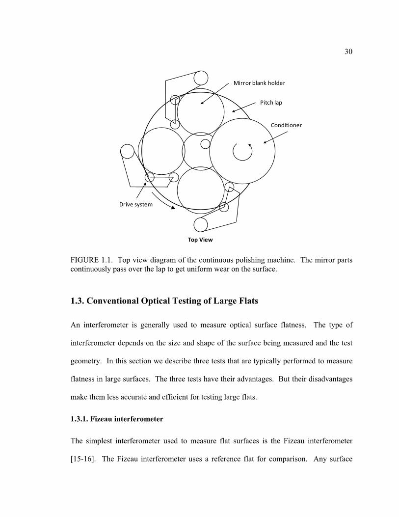
1.2. Current State of the Art for Flat Fabrication

The current state of the art for flat mirror fabrcation uses continuous polisher (CP)

machines, which can produce flat surfaces that are 30 nm rms [10-14]. The CP uses a

large annular lap that is at least three times the size of the part being polished and turns

continuously. A top view diagram of a CP machine is shown in Figure 1.1. The parts to

be polished are placed front surface down on the lap in holders that are fixed in place on

the annulus and are driven so they turn in synchronous motion with the lap. Because the

part is in synchronous motion with the lap, the part always remains in full contact with

the lap, so the wear on the part will be uniform. The uniform contact and wear allows the

surface to become flat rapidly. A conditioner that is as large as the radius of the lap helps

keep the lap flat through the long polishing operation.

There are two advantages of using CP machines: 1) they can produce multiple

flat mirrors simultaneously, making this type of a machine very cost-effective, and 2)

they can polish smoothly out to the mirror edges because of the uniform contact between

the mirror and the lap. The disadvantage, however, is that mirrors polished on a CP

machine can be no larger than about a third of the diameter of the lap. CP machines with

4 m diameter laps are known to exist [13]. These particular CP machines can only

accommodate up to 1.3 m flat mirrors. Any mirror bigger than 1.3 m has to be made with

conventional methods.

30

FIGURE 1.1. Top view diagram of the continuous polishing machine. The mirror parts continuously pass over the lap to get uniform wear on the surface.

1.3. Conventional Optical Testing of Large Flats

An interferometer is generally used to measure optical surface flatness. The type of

interferometer depends on the size and shape of the surface being measured and the test

geometry. In this section we describe three tests that are typically performed to measure

flatness in large surfaces. The three tests have their advantages. But their disadvantages

make them less accurate and efficient for testing large flats.

1.3.1. Fizeau interferometer

The simplest interferometer used to measure flat surfaces is the Fizeau interferometer

[15-16]. The Fizeau interferometer uses a reference flat for comparison. Any surface

Pitch lap

Conditioner

Mirror blank holder

Drive system

Top View

31

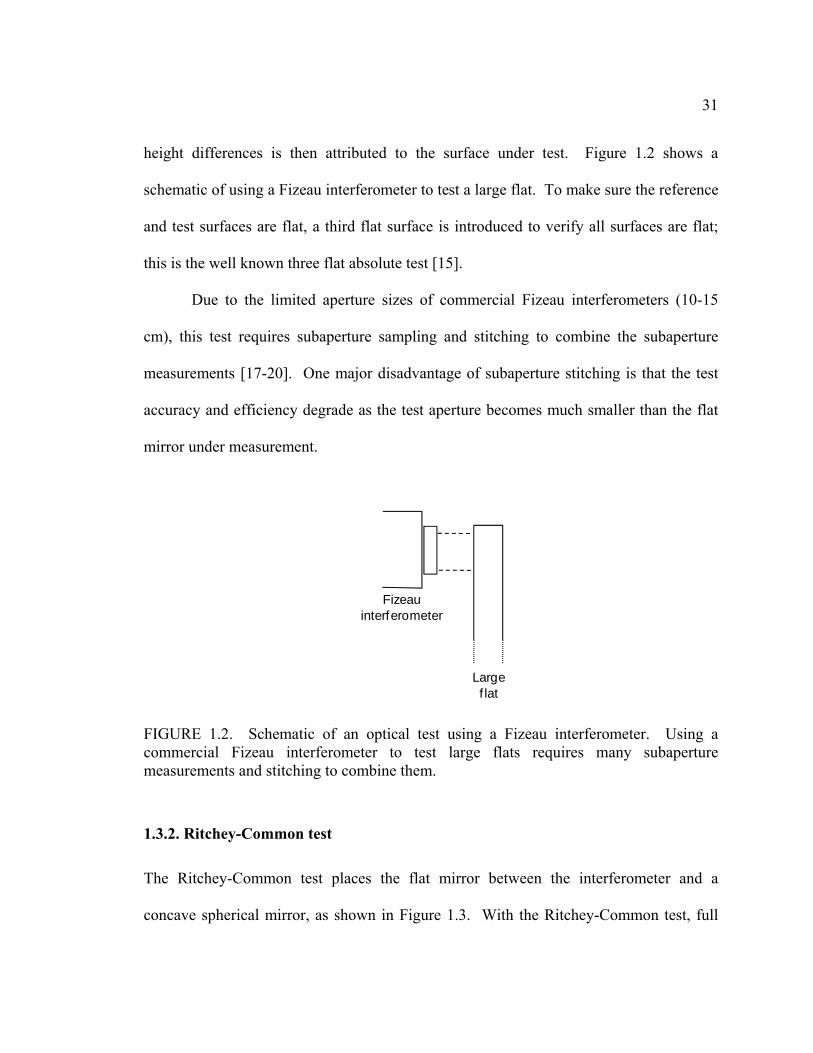
height differences is then attributed to the surface under test. Figure 1.2 shows a

schematic of using a Fizeau interferometer to test a large flat. To make sure the reference

and test surfaces are flat, a third flat surface is introduced to verify all surfaces are flat;

this is the well known three flat absolute test [15].

Due to the limited aperture sizes of commercial Fizeau interferometers (10-15

cm), this test requires subaperture sampling and stitching to combine the subaperture

measurements [17-20]. One major disadvantage of subaperture stitching is that the test

accuracy and efficiency degrade as the test aperture becomes much smaller than the flat

mirror under measurement.

FIGURE 1.2. Schematic of an optical test using a Fizeau interferometer. Using a commercial Fizeau interferometer to test large flats requires many subaperture measurements and stitching to combine them.

1.3.2. Ritchey-Common test

The Ritchey-Common test places the flat mirror between the interferometer and a

concave spherical mirror, as shown in Figure 1.3. With the Ritchey-Common test, full

Large f lat

Fizeauinterferometer

32

surface testing of the large flat is possible. The test measures concavity (or convexity)

accurately in the large flat mirror under test by measuring astigmatism in the surface [16,

21]. Surface irregularity, however, is more difficult to measure because the wavefront

falls off with the cosine of the angle of incidence.

( )θδ cos4=W (1.1)

where δ is the surface error height. The beam is reflected off the flat surface twice so

there is a factor of four in the measured wavefront. The difficulty comes from the angle,

θ, changing across the flat surface. In addition, the sensitivity to surface irregularity

decreases as the angle is increased.

FIGURE 1.3. Schematic of a Ritchey-Common optical test. The Ritchey-Common test uses a large spherical reference surface and is typically performed on large flats.

The advantage of the Ritchey-Common test over the Fizeau test is that it does not

require a reference flat surface for comparison. The disadvantage is, although easy to

Large f lat

Reference spherical mirror

Interferometer focus

θ

33

make, the spherical mirror must be larger than the flat mirror under test. Moving large

optics around the shop, mounting them, and aligning them are not easy tasks. Therefore,

the Ritchey-Common test is difficult and time consuming for very large mirrors.

1.3.3. Skip flat test

A less documented and relatively unknown test of large flat mirrors is the skip flat test

[22, 30]. This test uses an interferometer with a collimated output that is much smaller

than the test surface. The collimated beam is reflected from the test surface at an oblique

angle. The beam is returned with a flat mirror to provide a narrow profile of the mirror.

A schematic of the test geometry is shown in Figure 1.4. There is an anamorphic

magnification between the long and short axes of the beam footprint at the test surface.

Multiple measurements taken in different directions can be performed to determine the

figure of the test surface. The skip flat test is similar to the Ritchey-Common test; the

measured wavefront is multiplied by a factor of four due to the double reflection and falls

off as the cosine of the angle of incidence (Equation 1.1), where the cosine of the angle of

incidence in the skip flat test is the ratio of the diameters of the return flat and the large

test flat.

The skip flat test has been used where conventional surface testing was difficult to

perform (e.g. a cryogenic test of large mirrors). Like other stitching tests, however,

accuracy and efficiency suffer as the size of the measured subaperture decreases with

respect to the size of the mirror under test [17, 20].

34

FIGURE 1.4. Schematic of a skip flat optical test. The skip flat test is performed on large flats.

InterferometerReturn

f lat

Large f latBeam footprint

θ

35

SECTION I

ADVANCED TESTING TECHNOLOGIES

The first section presents testing technologies that were developed, analyzed, and

implemented during the manufacture of a 1.6 meter flat mirror. We developed two slope

tests, electronic levels and scanning pentaprism, and a 1 meter vibration insensitive

interferometer based on the classical Fizeau interferometer. The electronic levels were

used during the early stage of fabrication to measure global surface changes in the flat.

The scanning pentaprism and the 1 m Fizeau interferometer are highly accurate tests that

were used to guide the remaining fabrication and qualify the final surface figure of the

1.6 meter flat.

Two electronic levels, described in Chapter 2, provided an easy and efficient

slope test to guide surface grinding and coarse polishing. An algorithm was developed to

reduce the measured slope data and obtain surface maps represented by Zernike

polynomials. With the electronic levels the surface of the 1.6 m mirror can be measured

to 50 nm rms of low order aberrations.

The scanning pentaprism system, described in Chapter 3, has been used

successfully to test paraboloidal mirrors at the University of Arizona. By replacing the

beam projector and position detector with a high resolution electronic autocollimator and

carefully aligning the two pentaprisms to the autocollimator, this test system can be used

36

to test large flat surfaces to 9 nm rms power by performing diagonal line scans. The test

system has the option of measuring other low and mid order Zernike aberrations and only

θ dependent aberrations, which are obtained by performing circumferential scans where

both pentaprisms are fixed and the test mirror continuously rotates underneath.

The vibration insensitive Fizeau interferometer, described in Chapter 4, used 1 m

subaperture sampling to measure surface irregularity. By using two different techniques

(stitching and maximum likelihood estimation) the subaperture measurements were

combined to produce a full synthetic surface map. This test relied on multiple

overlapping subaperture measurements and measurement redundancy to isolate the errors

in the reference flat and the test flat to 3 nm rms.

37

CHAPTER 2

OPTICAL FLATNESS MEASUREMENTS USING ELECTRONIC

LEVELS

Conventional measurement methods for large flat mirrors are generally difficult and

expensive. In most cases, comparison with a master or a reference flat similar in size is

required. Using gravity, such as in modern pendulum-type electronic levels, takes

advantage of a free reference to precisely measure inclination. We describe using two

electronic levels to measure flatness of large flat mirrors. Using two levels differentially

allows surface slope measurements of large flat mirrors by removing common tilt

between the levels. One level is fixed, while the other level is moved across the mirror

surface. We provide measurement results on a 1.6 meter flat mirror. Our method of

measurement and data reduction resulted in measurement of surface accuracy to 50 nm

rms.

2.1. Introduction

Traditionally, large flat mirror testing can be difficult and expensive. The Ritchey-

Common test (described in Chapter 1), for example, requires a reference spherical mirror

larger in size than the test surface. The test is straight forward on a smaller scale;

however, aligning large optical components is a difficult and time consuming process.

38

The impact on schedule makes this test expensive for large optics. To overcome this

problem, we introduce a simple and cost effective slope test that uses two high precision

electronic levels.

Since the mid-1900’s techniques have been developed to measure flatness of

surfaces, namely industrial surface plates [23]. Methods to estimate the uncertainty in the

measurements to calibrate the surface plates have also been developed [23-24]. The first

measurement instruments included an analog autocollimator with a sliding mirror aligned

to the autocollimator. The autocollimator measured angle deviations in the surface by

sliding the mirror along measurement lines over the surface plate. Height profiles were

obtained by integrating the measured angle deviations or slopes. In the 1990’s high

precision electronic levels were introduced and became commercially available. The

measuring principle of electronic levels is based on a friction free pendulum suspended

between two electrodes. A deflection to the pendulum changes capacitance between the

electrodes, which is detected by a transducer and translated to an angle reading. Due to

their ease of use and cost effectiveness the electronic levels replaced the autocollimator

and mirror for measuring flatness of surfaces. One benefit of electronic levels is that

their use does not require the skill needed to operate an autocollimator. Also, the angle

readings can be recorded from a digital display or an acquisition system, which is a major

advantage over the time consuming process of manual data recording.

At the University of Arizona Optical Engineering and Fabrication Facility (UA-

OEFF), we extended the concept of measuring flatness of surface plates to optical

surfaces. A significant advantage of using electronic levels for surface measurements of

39

large mirrors during fabrication is that the mirror can remain on the polishing supports.

In contrast, other types of test systems may require moving the test mirror to a testing

fixture. In addition to measurement efficiency, their ease of use and cost effectiveness

make the electronic levels ideal for flatness measurements of large mirrors during

manufacturing.

The concept of using uni-axis electronic levels for large flat mirror measurements

is first introduced in Section 2.2. Section 2.3 provides the measurement sensitivities and

the error analysis. Next, Section 2.4 provides results of flatness measurements on a 1.6 m

flat mirror. In Section 2.5 a comparison of the electronic levels and the scanning

pentaprism tests is performed and the results are provided. Section 2.6 describes a

conceptual implementation of dual-axis electronic levels for flatness measurements on

large flat mirrors. A Monte Carlos simulation of dual-axis electronic levels for surface

measurements is also presented. Finally, the concluding remarks are provided in Section

2.7.

2.2. Test Concept

2.2.1. High precision electronic levels measurement system

A single high precision electronic level measures inclination of a surface, α, very

accurately, as shown schematically in Figure 2.1. Two levels used differentially allows

for surface slope measurements along the pointing direction where one level provides the

reference measurement, B, and the other level provides measurement A. The differential

measurement is the difference in the angular reading of the two instruments, A – B. The

40

reference level is normally fixed while level A is moved over the surface maintaining the

common pointing of both levels. Typically, this mode of measurement is used to

measure flatness of surface plates. In our case, we measure the flatness of large mirrors.

FIGURE 2.1. Schematic of the set up for measuring surface inclination with the electronic level.

Two high precision uni-axis electronic levels (Leveltronic NT made by Wyler AG

[25]) were procured along with the necessary hardware and electronics. Uni-axis, as

opposed to dual axis, levels can only measure inclination in the pointing direction. The

standard steel base plates were replaced with custom aluminum plates and three tungsten

carbide half-spheres for surface contact, as shown in Figure 2.2.

Maintaining the pointing of both levels is important when measuring flatness of

large mirrors. To ensure single line scans, a fiberglass guide rail was fabricated to fit

over the flat mirror as shown in Figure 2.3. The guide rail ensured consistent pointing of

the levels, and also provided repeatable measurement locations.

Gravity vector

α

αNormal to surface

(-n)

Pointing direction

Electronic level

41

FIGURE 2.2. A Wyler Leveltronic NT electronic level with a custom aluminum three-point base plate for stable positioning.

FIGURE 2.3. Top view of the electronic levels measurement set up for flatness measurements. A fiberglass guide rail secured to the mirror maintained the pointing of the electronic levels.

2.2.2. Principles of operation

To measure surface slopes the two levels were always used differentially. In this mode,

the reference level remained fixed anywhere along the guide rail while the other level

Electronic level

Custom base plate with three half

spheres

B A

Reference level

Scanning level

Guide rail

Large f lat mirror

x

y

42

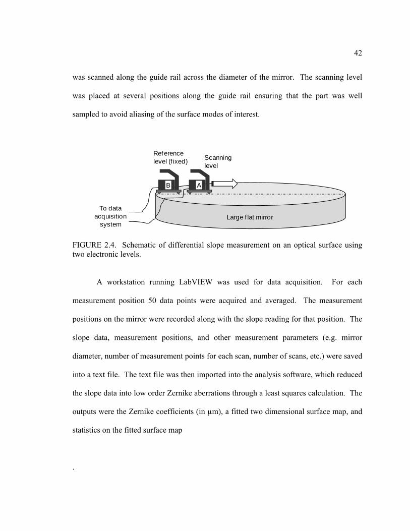
was scanned along the guide rail across the diameter of the mirror. The scanning level

was placed at several positions along the guide rail ensuring that the part was well

sampled to avoid aliasing of the surface modes of interest.

FIGURE 2.4. Schematic of differential slope measurement on an optical surface using two electronic levels.

A workstation running LabVIEW was used for data acquisition. For each

measurement position 50 data points were acquired and averaged. The measurement

positions on the mirror were recorded along with the slope reading for that position. The

slope data, measurement positions, and other measurement parameters (e.g. mirror

diameter, number of measurement points for each scan, number of scans, etc.) were saved

into a text file. The text file was then imported into the analysis software, which reduced

the slope data into low order Zernike aberrations through a least squares calculation. The

outputs were the Zernike coefficients (in µm), a fitted two dimensional surface map, and

statistics on the fitted surface map

.

Large f lat mirror

Reference level (f ixed) Scanning

level

AB

To data acquisition

system

43

2.2.3. Fit using Zernike polynomials

Since the electronic levels measured slope change, we performed the analysis using a

basis set of slope functions derived from the Zernike polynomials. If the surface error is

described by

( ) ( )∑= yxZayxS ii ,, (2.1)

where iZ are the Zernike polynomials in Cartesian coordinates and ia are their

coefficients, and measurements made in a direction is defined by

θθ sinjcosi + , (2.2)

then the slope data can be expressed as

( ) ( ) ( )∑ +⋅∇= θθθα sinjcosi,,, yxZayx ii

v, (2.3)

where ( )yxZi ,∇v

is the gradient of the Zernike polynomials and forms a dot product with

the measurement direction. The low order Zernike aberrations and their gradients are

shown in Table 2.1.

The analysis software creates a matrix of low order slopes and a vector of

measured surface slopes. Through a least squares calculation, the Zernike coefficients

are determined by

[ ] [ ] [ ]'\ za α= , (2.4)

where [ ]'z is a matrix of gradients of the Zernike polynomials projected in the

measurement direction

[ ]α is a vector of measured slope variations across the mirror surface.

44

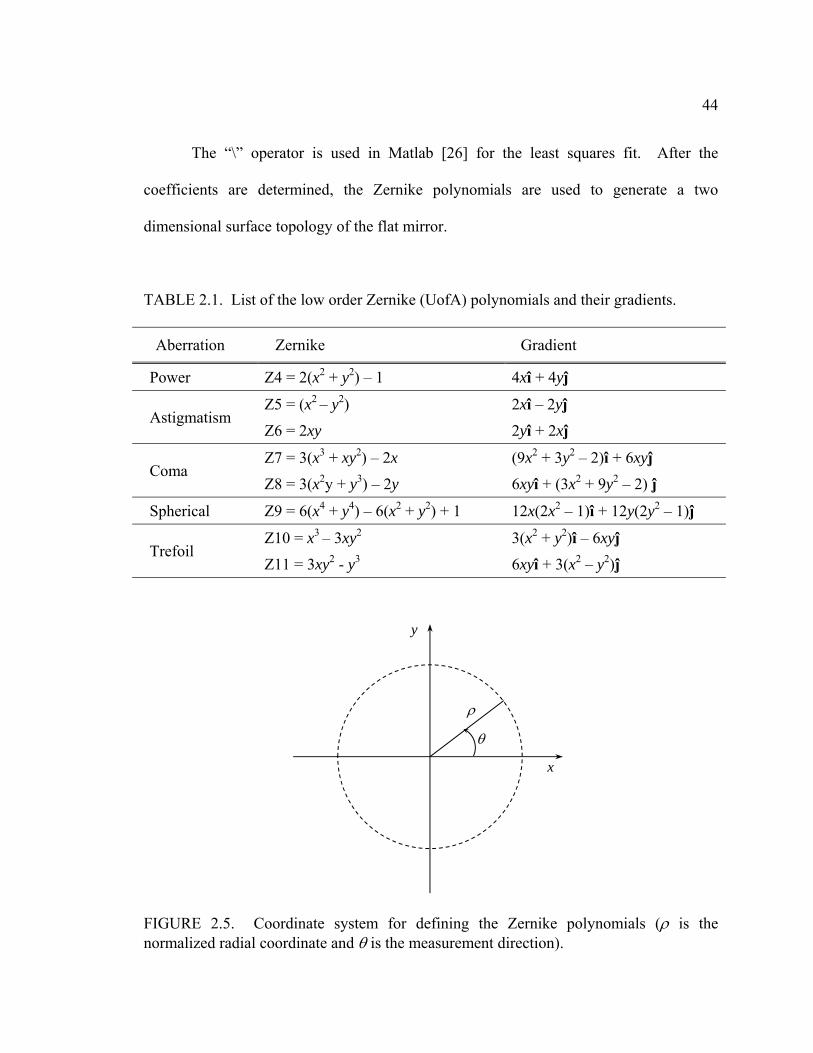
The “\” operator is used in Matlab [26] for the least squares fit. After the

coefficients are determined, the Zernike polynomials are used to generate a two

dimensional surface topology of the flat mirror.

TABLE 2.1. List of the low order Zernike (UofA) polynomials and their gradients.

Aberration Zernike Gradient

Power Z4 = 2(x2 + y2) – 1 4xî + 4yĵ

Astigmatism Z5 = (x2 – y2) 2xî – 2yĵ

Z6 = 2xy 2yî + 2xĵ

Coma Z7 = 3(x3 + xy2) – 2x (9x2 + 3y2 – 2)î + 6xyĵ

Z8 = 3(x2y + y3) – 2y 6xyî + (3x2 + 9y2 – 2) ĵ

Spherical Z9 = 6(x4 + y4) – 6(x2 + y2) + 1 12x(2x2 – 1)î + 12y(2y2 – 1)ĵ

Trefoil Z10 = x3 – 3xy2 3(x2 + y2)î – 6xyĵ

Z11 = 3xy2 - y3 6xyî + 3(x2 – y2)ĵ

FIGURE 2.5. Coordinate system for defining the Zernike polynomials (ρ is the normalized radial coordinate and θ is the measurement direction).

x

y

ρ

θ

45

2.3. Analysis

2.3.1. Sensitivity analysis: sampling for low order Zernike aberrations

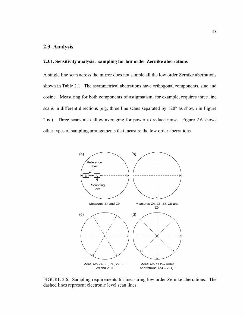
A single line scan across the mirror does not sample all the low order Zernike aberrations

shown in Table 2.1. The asymmetrical aberrations have orthogonal components, sine and

cosine. Measuring for both components of astigmatism, for example, requires three line

scans in different directions (e.g. three line scans separated by 120° as shown in Figure

2.6c). Three scans also allow averaging for power to reduce noise. Figure 2.6 shows

other types of sampling arrangements that measure the low order aberrations.

FIGURE 2.6. Sampling requirements for measuring low order Zernike aberrations. The dashed lines represent electronic level scan lines.

B A

Reference level

Scanning level

Measures Z4 and Z9. Measures Z4, Z5, Z7, Z8 and Z9.

Measures Z4, Z5, Z6, Z7, Z8, Z9 and Z10.

Measures all low order aberrations (Z4 – Z11).

(a) (b)

(c) (d)

46

Scans through the center of the mirror are not a requirement. The scans can be

offset from center; the aberrations measured still hold for the number of line scans made.

The mirror surface should be well sampled along each scan line to avoid aliasing of the

surface modes. For example, we periodically sampled for secondary spherical aberration.

Sampling for secondary spherical requires a minimum of five measurement points across

the diameter of the mirror, but this leaves a large measurement uncertainty for secondary

spherical due to noise (discussed in more detail in Chapter two). More measurement

points across the mirror will reduce the uncertainty.

Figures 2.7 and 2.8 show how the slope measurements would appear for the low

order aberrations if the three line scans (at 0°, 120°, and 240°) shown in Figure 2.6c were

performed. The plots are normalized by assuming the Zernike wavefront coefficients are

1 µm. The amount of each low order term is determined using the least squares fit to the

measured slope data.

The three line scans have excellent sensitivities to the low order aberrations,

except for Zernike 11 (sin trefoil). Trefoil is, thus, not adequately sampled with the three

line scans. To fix this, four line scans shown in Figure 2.6d is required. To avoid

aliasing, a minimum of three measurement points across the mirror diameter is required

to measure all the low order aberrations (spherical aberration requires the most number of

measurement points). But as pointed out previously, the measurement uncertainty due to

noise will be high for a small number of measurement points.

47

FIGURE 2.7. Simulated three line scans (separated by 120°) for low order surface errors described by single Zernike polynomial terms (power, astigmatism, and spherical aberrtaion).

48

FIGURE 2.8. Simulated three line scans (separated by 120°) for low order surface errors described by single Zernike polynomial terms (coma and trefoil).

2.3.2. Error analysis

Drescher [20] reported on a method for estimating uncertainty in the surface slope

measurements of industrial surface plates. We applied a similar analysis for measuring

optical surfaces. The error sources can be separated into two categories: random and

systematic errors. The random errors can be controlled through data averaging. The

49

systematic errors are fixed and cannot be eliminated, but they may be minimized after

characterizing them.

FIGURE 2.9. Measured noise in the electronic levels after removing linear drift (1σ = 0.15 μrad). Sample period = 3.3 Hz (full rate).

Random errors:

1. There is inherent noise associated with the electronic levels. We measured the noise

floor of the levels to less than 0.2 µrad. The plot in Figure 2.9 shows a typical

continuous measurement exhibiting noise after removing the drift effect. The continuous

measurement was performed over one hour at the full sampling rate of the device (3.3

Hz) in the same environment in which the optical surface slope measurements were

performed.

50

2. There was drift observed in the measurements due to environmental effects, notably

thermal. The magnitude and direction of the drift seemed to be random in nature. The

plot in Figure 2.10 represents a typical continuous measurement that shows drift and

noise. The levels were placed on a flat rigid surface and allowed to settle and equilibrate

for one hour. Measurements were then continuously taken over another hour at the full

sampling rate of the device.

FIGURE 2.10. Measured drift and noise over 60 minutes. The amount of drift is about 1.75 μrad over 60 min (30 nrad/min).

The plot shows the level drifted about 1.75 µrad over 60 minutes or 30 nrad per

minute. To minimize the drift effect, a reference measurement was always acquired that

accompanied the data point. The reference measurement was then subtracted from the

data. The two measurements were acquired in rapid succession that was much less than

51

the time constant of the drift. For example, a full measurement performed at one position

on the mirror in three minutes introduced about 90 nrad of error.

3. The fiberglass guide rail used to maintain the pointing of the levels was not perfectly

straight. The straightness was specified to less than 0.5 mm/m. This caused an error in

pointing and coupling of the reading between the orthogonal axes, thus the slope error in

the x direction became

θαα Δ×=Δ yx , (2.5)

where αy is the slope in y

Δθ is the error in pointing (0.5 mrad).

For a ground mirror surface, the slopes can vary by no more than 4 nrad per mm.

The contact point spacing of the electronic levels in the y direction was 64 mm, thus the

slope in y vared by 256 nrad. The error in the slope reading in the x direction was then

0.13 µrad.

4. The slope error due to placement and setting of the levels is described by

2/122

dd

dd

dd

⎥⎥⎦

⎤

⎢⎢⎣

⎡⎟⎟⎠

⎞⎜⎜⎝

⎛+⎟

⎠⎞

⎜⎝⎛=Δ y

yx

xyx αα

α . (2.6)

The fiberglass guide rail helped constrain the placement of the levels to 2 mm in

the pointing direction x and to 0.5 mm in the y direction. If the surface slopes varied by 4

nrad/mm, then the placement error caused about 8 nrad in the measurement direction.

52

5. The residual error from the slope fit calculation consistently introduced an uncertainty

of about 0.13 µrad. This error can be reduced by including more measurement points

across the mirror.

Systematic errors:

There is only one systematic error to consider.

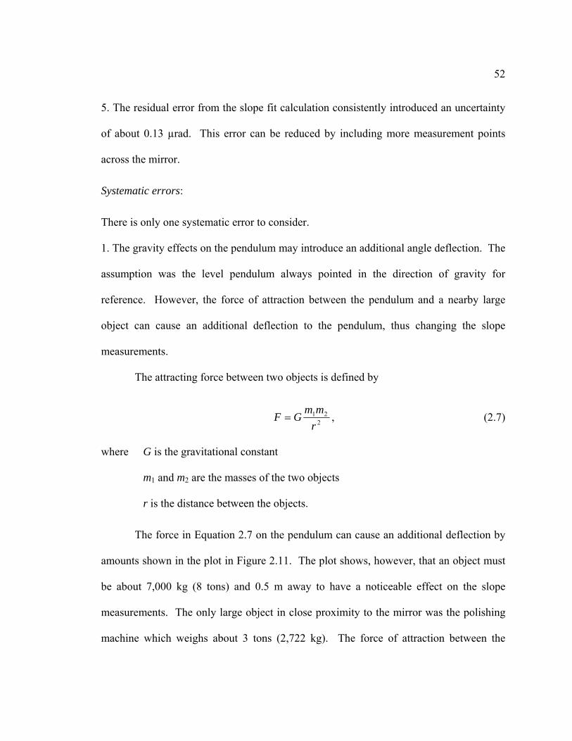
1. The gravity effects on the pendulum may introduce an additional angle deflection. The

assumption was the level pendulum always pointed in the direction of gravity for

reference. However, the force of attraction between the pendulum and a nearby large

object can cause an additional deflection to the pendulum, thus changing the slope

measurements.

The attracting force between two objects is defined by

221

rmmGF = , (2.7)

where G is the gravitational constant

m1 and m2 are the masses of the two objects

r is the distance between the objects.

The force in Equation 2.7 on the pendulum can cause an additional deflection by

amounts shown in the plot in Figure 2.11. The plot shows, however, that an object must

be about 7,000 kg (8 tons) and 0.5 m away to have a noticeable effect on the slope

measurements. The only large object in close proximity to the mirror was the polishing

machine which weighs about 3 tons (2,722 kg). The force of attraction between the

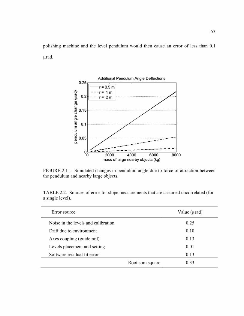
53

polishing machine and the level pendulum would then cause an error of less than 0.1

µrad.

FIGURE 2.11. Simulated changes in pendulum angle due to force of attraction between the pendulum and nearby large objects.

TABLE 2.2. Sources of error for slope measurements that are assumed uncorrelated (for a single level).

Error source Value (μrad)

Noise in the levels and calibration 0.25

Drift due to environment 0.10

Axes coupling (guide rail) 0.13

Levels placement and setting 0.01

Software residual fit error 0.13

Root sum square 0.33

54

Table 2.2 shows a summary of the error sources and their values. A root sum

square (RSS) of all the error sources that are uncorrelated is about 0.33 µrad for a single

level. The error from gravity effects then limits the accuracy of the level to about 0.4

µrad.

A Monte Carlo simulation of the three line scans (shown in Figure 2.6c) on a 2 m

flat mirror was performed to determine the sensitivities of the low order Zernike

aberrations using an uncertainty of 0.56 µrad for a single differential measurement. This

analysis assumed 12 measurement points per scan. From the result of the simulation, the

measurement uncertainty of each of the low order aberrations can be estimated. Table

2.3 shows that the expected accuracy for the measurement of a 2 m flat mirror is 50 nm

rms of low order aberrations.

TABLE 2.3. Measurement uncertainty for the low order Zernike aberrations with the uni-axis levels.

Zernike aberration Measurement uncertainty (nm rms)

Power 16

Cos Astigmatism 29

Sin Astigmatism 29

Cos Coma 11

Sin Coma 11

Spherical 8

Secondary Spherical 6

Root sum square 50

55

2.3.3. Other scanning arrangements for uni-axis electronic levels

There are other possible scanning arrangements for measuring surface slopes in large flat

mirrors using uni-axis electronic levels. Figure 2.12 shows orthogonal scans with up-

down (a) and left-right (b) pointing directions. The data analysis remains the same for

these scanning arrangements. These types of scanning arrangements were not performed

during this work.

FIGURE 2.12. Orthogonal scans with up-down (a) and left-right (b) pointing directions using uni-axis electronic levels.

B

A

A

scan

B

A A

scan

1 2

Large f lat mirror

B

A

A

scan

B

A A

scan

1 2

Large f lat mirror

(a)

(b)

56

2.4. Measurement of a 1.6 Meter Flat Mirror

2.4.1. Single line scan

A single line scan, as shown in Figure 2.6a, provides information only on symmetrical

aberrations (e.g. power). Figure 2.13 shows the result of a single line scan on the 1.6 m

mirror while in was in production. The top left plot (2.13a) shows the measured surface

slopes with 12 measurement points and a fit to them using slope functions for power and

spherical. The bottom left plot (2.13b) shows the surface profile in microns after

determining the Zernike coefficients. The right plot (2.13c) shows the two dimensional

fitted surface map and the scan made on the mirror. All of the plots are normalized in

radius.

FIGURE 2.13. (a) Low order symmetrical Zernike aberrations fitted to measured slope data. (b) Surface profile of the fitted surface map. (c) The corresponding two dimensional fitted surface map with 680 nm PV and 160 nm rms.

57

The results shown in Figure 2.13 yielded an overall surface error of 160 nm rms:

127 nm rms was attributed to power and 128 nm rms to spherical.

2.4.2. Three Line Scans

The three line scans, as shown in Figure 2.6c, provide information on all the low order

Zernike aberrations, except for trefoil. Figure 2.14a shows the result of the three line

scans on the same 1.6 m flat mirror (at an earlier time in the fabrication process) and fits

to them using slope functions of the low order Zernike polynomials. For this set of

measurements we did not sample the center of the mirror.

Figure 2.14b shows the generated two-dimensional surface map and the line scans

after the least squares calculation of the Zernike coefficients. The resulting surface map

shown in Figure 2.14b yielded 295 nm rms of overall surface error. Table 2.4 shows a

breakdown of error contributions from the low order aberrations.

58

FIGURE 2.14. (a) Fit to measured surface slopes along three line separated by 120°. (b) The resulting surface map of the three line scan (295 nm rms).

TABLE 2.4. Values of the low order Zernike coefficients after fit to surface slopes.

Zernike Aberration Value (nm rms)

Power 280

Cos Astigmatism -97

Sin Astigmatism 33

Cos Coma -65

Sin Coma 6

Spherical -141

59

2.5. Comparison of the Electronic Levels and Scanning Pentaprism Tests

This section presents the results of the comparison of the electronic levels and the

scanning pentaprism test. Both test systems measured surface slopes with the scanning

pentaprism providing higher measurement accuracy. To validate the measurements with

the electronic levels, the 1.6 m flat was measured with both test systems while the mirror

was in early production. The same direction on the mirror was measured and 10

measurement points were acquired with both test systems. The sampling spacing

between the two systems differed, however.

Figure 2.15 shows the results from the electronic levels test, and Figure 2.16

shows the results from the scanning pentaprism test. Table 2.5 shows (for comparison)

the surface statistics from both tests after power and spherical aberration were fit to the

slope data. Table 2.6 shows the difference in the data from both tests.

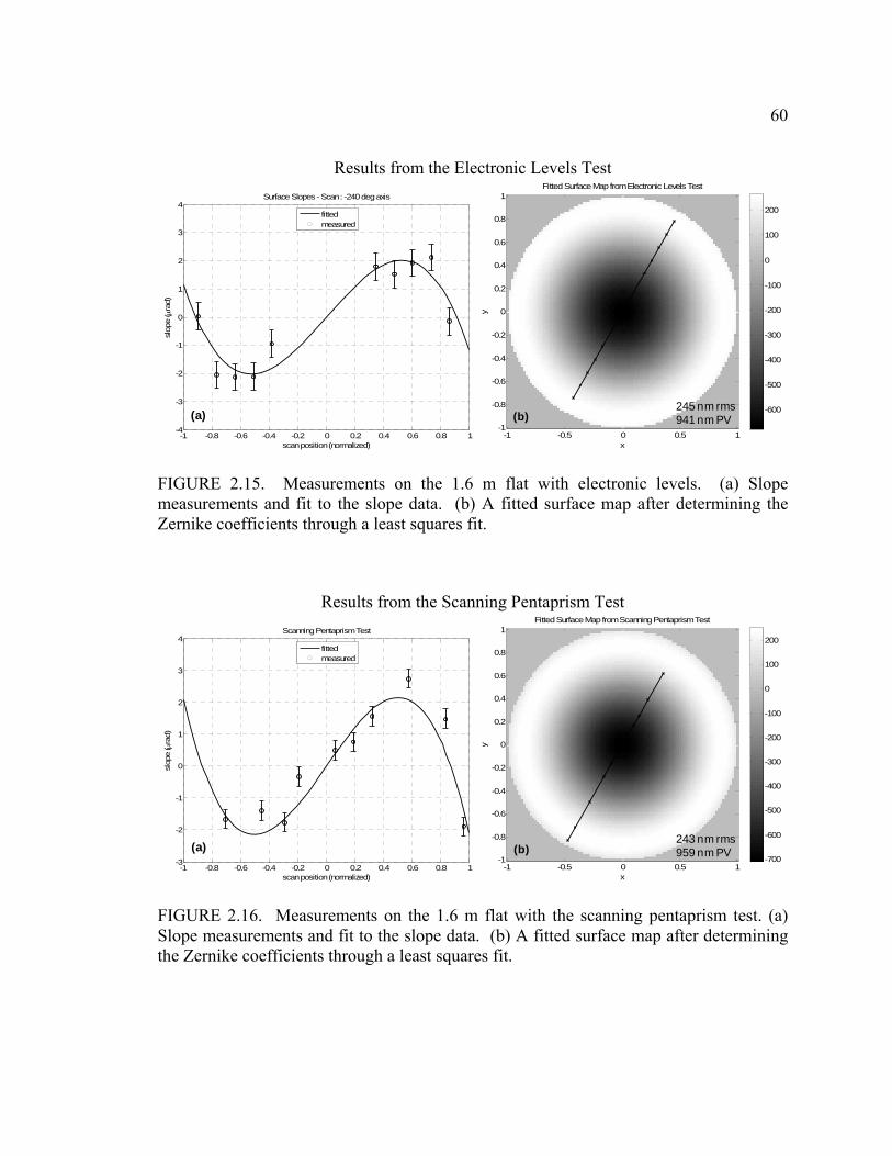
60

Results from the Electronic Levels Test

FIGURE 2.15. Measurements on the 1.6 m flat with electronic levels. (a) Slope measurements and fit to the slope data. (b) A fitted surface map after determining the Zernike coefficients through a least squares fit.

Results from the Scanning Pentaprism Test

FIGURE 2.16. Measurements on the 1.6 m flat with the scanning pentaprism test. (a) Slope measurements and fit to the slope data. (b) A fitted surface map after determining the Zernike coefficients through a least squares fit.

-1 -0.8 -0.6 -0.4 -0.2 0 0.2 0.4 0.6 0.8 1-4

-3

-2

-1

0

1

2

3

4Surface Slopes - Scan : -240 deg axis

scan position (normalized)

slop

e ( μ

rad)

fittedmeasured

(a)(a)

Fitted Surface Map from Electronic Levels Test

x

y

-1 -0.5 0 0.5 1-1

-0.8

-0.6

-0.4

-0.2

0

0.2

0.4

0.6

0.8

1

-600

-500

-400

-300

-200

-100

0

100

200

245 nm rms941 nm PV(b)

-1 -0.8 -0.6 -0.4 -0.2 0 0.2 0.4 0.6 0.8 1-3

-2

-1

0

1

2

3

4Scanning Pentaprism Test

scan position (normalized)

slop

e ( μ

rad)

fittedmeasured

(a)

Fitted Surface Map from Scanning Pentaprism Test

x

y

-1 -0.5 0 0.5 1-1

-0.8

-0.6

-0.4

-0.2

0

0.2

0.4

0.6

0.8

1

-700

-600

-500

-400

-300

-200

-100

0

100

200

243 nm rms959 nm PV(b)

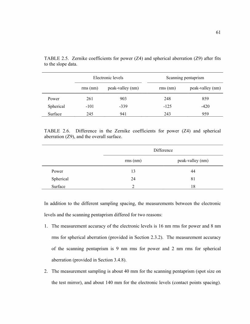
61

TABLE 2.5. Zernike coefficients for power (Z4) and spherical aberration (Z9) after fits to the slope data. Electronic levels Scanning pentaprism

rms (nm) peak-valley (nm) rms (nm) peak-valley (nm)

Power 261 903 248 859

Spherical -101 -339 -125 -420

Surface 245 941 243 959 TABLE 2.6. Difference in the Zernike coefficients for power (Z4) and spherical aberration (Z9), and the overall surface. Difference

rms (nm) peak-valley (nm)

Power 13 44

Spherical 24 81

Surface 2 18

In addition to the different sampling spacing, the measurements between the electronic

levels and the scanning pentaprism differed for two reasons:

1. The measurement accuracy of the electronic levels is 16 nm rms for power and 8 nm

rms for spherical aberration (provided in Section 2.3.2). The measurement accuracy

of the scanning pentaprism is 9 nm rms for power and 2 nm rms for spherical

aberration (provided in Section 3.4.8).

2. The measurement sampling is about 40 mm for the scanning pentaprism (spot size on

the test mirror), and about 140 mm for the electronic levels (contact points spacing).

62

This causes the same effect as averaging the surface slopes over the measurement

sampling, but it is less of a problem for low order aberrations sampling.

The results of the comparison show that both test systems agree to within the

measurement accuracy of the electronic levels, thus validating the electronic levels

measurements.

2.6. Implementation with Dual Axis Electronic Levels

The scanning arrangements shown in Section 2.3.3 can be accomplished more efficiently

with dual axis electronic levels as shown in Figure 2.17. Dual axis levels can measure

two orthogonal axes simultaneously: the pointing direction and the direction orthogonal

to it. Although we did not procure dual axis levels during the work reported here, they

are available commercially. In this section, we analyze the performance of such levels

through Monte Carlo simulations assuming the same type of measurement accuracies for

both axes as for the uni-axis levels.

The data reduction remains the same for the dual axis levels. Slopes in

orthogonal directions will be known for each measurement point; the common pointing

of the levels must still be maintained. The errors contributing to uncertainty in the

measurement can be treated in the same manner as for the uni-axis levels. With dual axis

levels, measurements on a square grid can be made instead of scans through the center of

the mirror to take advantage of the slope information in orthogonal axes (Figure 2.18).

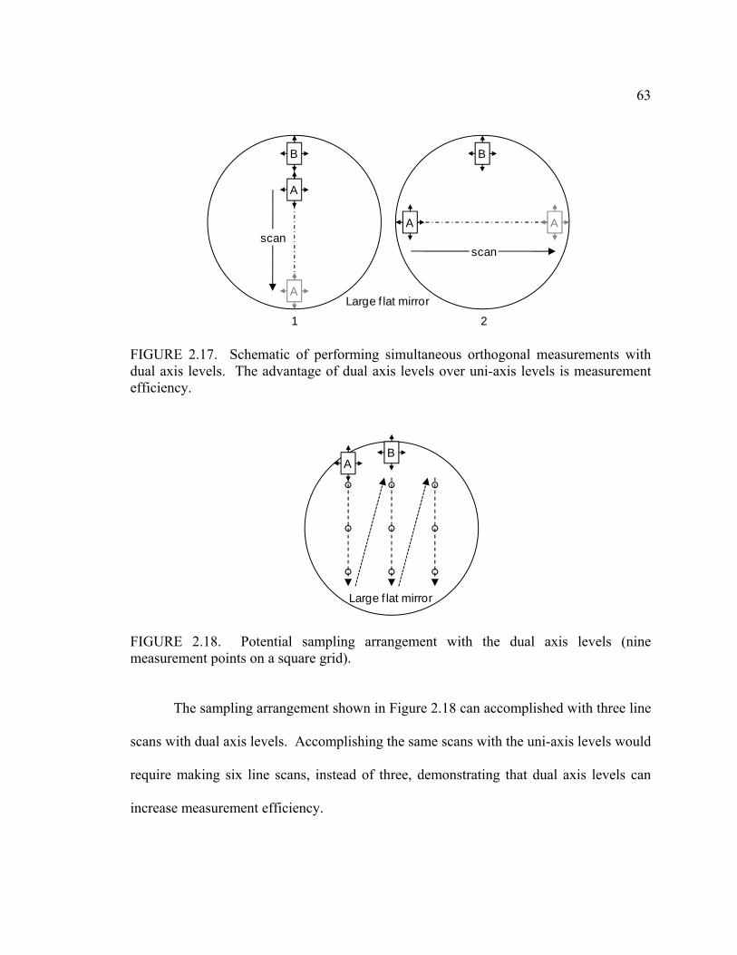
63

FIGURE 2.17. Schematic of performing simultaneous orthogonal measurements with dual axis levels. The advantage of dual axis levels over uni-axis levels is measurement efficiency.

FIGURE 2.18. Potential sampling arrangement with the dual axis levels (nine measurement points on a square grid).

The sampling arrangement shown in Figure 2.18 can accomplished with three line

scans with dual axis levels. Accomplishing the same scans with the uni-axis levels would

require making six line scans, instead of three, demonstrating that dual axis levels can

increase measurement efficiency.

B

A

A

scan

B

A A

scan

1 2

Large f lat mirror

BA

Large f lat mirror

64

Figure 2.19 shows the results of two measurement simulations with dual axis

electronic levels. The sampling arrangements with dual axis levels shown in Figure 2.19

do not adequately sample astigmatism. To fix this, additional measurements on a rotated

measurement grid is required.

FIGURE 2.19. A simulation result of dual axis levels measurement on a 3 × 3 (a) and 5 × 5 (b) square grids assuming the same level of measurement uncertainty as for the uni-axis levels.

The advantage provided by dual axis electronic levels is efficiency, providing

twice the information in a single measurement. Due to this fact, UA-OEFF is interested

in obtaining dual axis electronic levels to do flatness measurements on large flat mirrors

in the future.

2.7. Conclusion

The conventional measurement methods of large flat mirrors are often difficult and

expensive. We provided an analysis of a high precision electronic level measurement

65

system that uses gravity as a reference and measures flatness in large flat mirrors with an

option to measure other low order aberrations. The sources of error that limit the

accuracy of the system were quantified; the errors are minimized through data averaging,

using a guide rail, and making reference measurements. A Monte Carlo simulation of the

system performance was performed based on the measurement uncertainty estimated

from the error analysis. The simulation result showed the uncertainty in the measured

low order Zernike aberrations and measurements to 50 nm rms of low order aberrations

are achievable for 2 m class flat mirrors. The accuracy, efficiency, and low cost of the

test system are ideal for testing of large flat mirrors. This test system can be used to

guide polishing during the early stages of manufacture. In addition, the portability of the

test system allows the test flat to be tested on the polishing table without moving the test

flat to a testing fixture.

66

CHAPTER 3

ANALYSIS OF A SCANNING PENTAPRISM SYSTEM FOR

MEASUREMENTS OF LARGE FLAT MIRRORS

We present an absolute test used to determine shape errors in large flat mirrors by

measuring slope variations across the surface. The system uses two pentaprisms aligned

to a high resolution electronic autocollimator. The pentaprisms deflect the collimated

beam from the autocollimator nominally by 90° to the mirror surface, and the beam then

returns on itself. The collimated beam is scanned across the flat mirror using motion of

one of the pentaprisms on a linear stage. Any additional deflection in the return beam

from the scanning prism provides a direct measurement of the shape error in the mirror

surface. Misalignments and motions in the autocollimator and prisms that occur during

scanning introduce second order error influences to the return beam. An active feedback

system aids in maintaining the alignment of the prisms to minimize the error influences.

Using this methodology, we measured 11 nm rms power in a 1.6 meter diameter flat

mirror. The system can be used in a scanning or non-scanning mode, which measures

only θ dependent aberrations.

67

3.1. Introduction

This chapter describes and analyzes a highly accurate optical slope test for very large flat

mirrors. The test system consisted of a high resolution electronic autocollimator and two

pentaprisms. A second electronic autocollimator was used as part of an active feedback

control system to maintain the angular alignment of the scanning pentaprism during the

scanning operation.

In optical surface metrology, systems with pentaprism(s) are used where

conventional interferometric testing would otherwise be difficult or limited [27-28]. Two

commonly used methods for testing flat mirrors interferometrically are the Fizeau test

and the Ritchey-Common test. Both tests, described in Chapter 1, have limitations in

terms of size for the Fizeau test and difficulty in performing the test on large mirrors for

the Ritchey-Common test. We have developed a slope test system that overcomes these

limitations.

The scanning pentaprism test system is highly accurate for measuring flatness in

large flat mirrors. The system performance is limited in accuracy by second order error

influences due to coupling of misalignments and motions in the autocollimator,

pentaprisms, and test surface, and beam and prism errors coupling into lateral motion of

the scanning pentaprism. The system discussed in this chapter built on a previous

scanning system, which was designed to deflect the autocollimator beam upward to a flat

mirror suspended above the test site and used off the shelf hardware [27-28]. In contrast,

the new system deflected the collimated beam down to where the large test mirror rested

on stable mechanical supports and used custom hardware. In addition to custom

68

hardware, alignment and data analysis techniques were modified in an effort to make the

system more stable and accurate. The entire integrated test system, although heavy (~200

kg), is kinematic and can be transported by a hoist.

3.1.1. Systems with pentaprisms

Pentaprisms are used to deflect light beams at a constant angle (nominally by 90°)

regardless of its orientation in the line of sight direction. Various optical test systems and

devices involving pentaprisms make use of this unique property. Many systems

involving pentaprisms have been developed to measure optical surface errors by

measuring surface slopes [27-30]. Simply integrating the slope data gives surface height

profiles. Through multiple measurements of the optical surface in different directions, a

full synthetic surface map can be obtained. Other systems with pentaprisms are used to

aid in optical alignments or in optical recording heads. Sensitive optical alignments and

error corrections are made possible by the ability of the pentaprisms to project collimated

and nominally parallel reference beams onto optical surfaces. Efforts have been made to

understand the error influences in pentaprism systems [31-33]. Some systems have been

refined to make them more accurate and less sensitive to alignment and motion errors

[31-43].

The scanning pentaprism system design and development is presented in Section

3.2. This includes the system hardware, integration and alignment. The results and

performance for 1.6 m flat mirror measurements are presented in Section 3.3. Finally, an

analysis of error sources that limit the accuracy of the system and Monte Carlo analysis

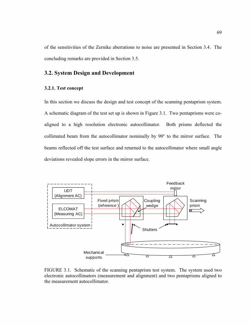
69

of the sensitivities of the Zernike aberrations to noise are presented in Section 3.4. The

concluding remarks are provided in Section 3.5.

3.2. System Design and Development

3.2.1. Test concept

In this section we discuss the design and test concept of the scanning pentaprism system.

A schematic diagram of the test set up is shown in Figure 3.1. Two pentaprisms were co-

aligned to a high resolution electronic autocollimator. Both prisms deflected the

collimated beam from the autocollimator nominally by 90° to the mirror surface. The

beams reflected off the test surface and returned to the autocollimator where small angle

deviations revealed slope errors in the mirror surface.

FIGURE 3.1. Schematic of the scanning pentaprism test system. The system used two electronic autocollimators (measurement and alignment) and two pentaprisms aligned to the measurement autocollimator.

ShuttersAutocollimator system

Fixed prism (reference )

Scanning prism

Feedback mirror

Mechanical supports

Coupling wedge

ELCOMAT(Measuring AC)

UDT(Alignment AC)

70

The system can be used in a scanning or non-scanning mode. In the scanning

mode, the reference prism remained fixed while the scanning prism was translated over

the mirror surface. Since the autocollimator can only measure one return signal at a time,

electronic shutters were used to alternately select the reference path and the scanning

path. By taking a difference between the two prisms, the measurements became

insensitive to the motion of the mirror or the autocollimator in the measurement direction

or pitch (defined in Figure 3.2). An integration of the slope data provided surface height

profiles along the scanning direction. The alternative method to integration is to fit low

order slope functions derived from the Zernike polynomials to the slope data through a

least squares calculation. The description of this method was given in Chapter two. Two

dimensional surface topology maps were then generated from the Zernike polynomials

after several scans at different orientations over the mirror.

In the non-scanning mode, both prisms remained fixed and the flat mirror under

test was rotated while data was acquired continuously. Typically, the reference prism

was positioned at one edge of the mirror, and the scanning prism was positioned at the

center of the mirror. The non-scanning mode measured only θ dependent aberrations

such as astigmatism (2θ) and trefoil (3θ).

The pentaprism system allowed slope determination only in the scan direction.

We call this direction the line of sight pitch or in-scan direction. The prism degrees of

freedom (pitch, yaw, and roll) are defined in Figure 3.2. Coupling between

misalignments and motions of the prisms, autocollimator, and test surface in these

degrees of freedom caused second order error influences to the beam line of sight.

71

Careful alignment of the scanning prism is required to minimize these errors. A second

autocollimator (UDT shown in Figure 3.1), aligned to a small return mirror attached to

the scanning pentaprism, was used to maintain the scanning pentaprism in angular

alignment through an active feedback control. Sources of line of sight errors up to

second order are listed in Table 3.1. The line of sight pitch varies linearly with the

autocollimator and test surface pitch angles, and quadratically with other angular

parameters. The first order effect of the autocollimator and test surface pitch motions

were common to both the fixed and scanning prisms, so it was eliminated by performing

differential measurements between the reference and scanning prisms.

FIGURE 3.2. Coordinate system and definition of the degrees of freedom for the autocollimator, scanning pentaprism and the test surface.

Auto-collimator

αTS

βAC

Scanning pentaprism

Test surface

x

y

z

α: pitchβ: yawγ: roll γTS

γAC γPP

αPPαAC βPP

72

TABLE. 3.1. Complete list of the line of sight alignment errors. Only the second order errors contribute to the in-scan slope error.

Contributions to line-of-sight pitch (in-scan direction)

Contributions to line-of-sight roll (cross-scan direction)

αAC βAC

αTS βPP

γPP2 γPP

γAC × γPP γTS

γAC × βPP αAC × βPP

γAC × γTS αAC × βTS

γTS × γPP αAC × γAC

γTS × βPP αAC × γPP α: pitch β: yaw γ: roll

AC: autocollimator PP: pentaprism TS: test surface

Pentaprism pitch motion sensitivity

Small pitch motion of the pentaprism was expected. This motion, however, had no effect

on the beam deviation in the in-scan direction. This is the beauty of the pentaprism: the

input beam is deviated at a constant (nominally) 90° angle, independent of small pitch

errors. We take advantage of this property. As mentioned previously, this property

makes the pentaprisms useful as reference beam projectors.

73

Pentaprism yaw and roll motion sensitivities

The in-scan (vertical) and cross-scan (horizontal) angles are coupled for yaw and roll

motions of the pentaprism. The dependence is linear for yaw motion and quadratic for

roll motion [31-33].

(a)

‐5‐3‐1135

‐250 ‐150 ‐50 50 150 250

AC vertical angle (μ

rad)

AC horizontal angle (μrad)

Pentaprism yaw scan

012345

‐250 ‐150 ‐50 50 150 250

AC vertical angle (μ

rad)

AC horizontal angle (μrad)

Pentaprism roll scan

(b) (c)

FIGURE 3.3. (a) Pentaprism yaw and roll scans. (b) Linear dependence of the angle measured with the autocollimator on the yaw angle of the prism. (c) Quadratic dependence of the angle measured with the autocollimator on the roll angle of the prism.

Any misalignments in yaw and roll couple with autocollimator, pentaprism, and

test surface motions to cause second order errors. If the pentaprism is aligned, however,

then the spot motion is the same for pentaprism roll and yaw motions. The in-scan

Auto-collimator

Test surface

Yaw scan

Roll scan

74

measurement is then perpendicular to the spot motion caused by motions in pentaprism

roll and yaw. The noise over the amount of motions in roll and yaw gives the accuracy of

the alignment. For example, if the yaw and roll alignments of the pentaprism are

maintained to 50 µrad, the line of sight pitch will vary by less than 10 nrad (shown in

Section 3.4.2).

Information from pentaprism yaw motion can be used to align both the

autocollimator roll and the prism roll (Section 3.2.4). Geckeler [31-33] derives the slope

of the autocollimator angle readings (vertical versus horizontal) from the yaw scan as

ACTSyawscan αα −=M , (3.1)

which reveals information on the difference of the roll angles of the autocollimator and

the test surface. The autocollimator roll is aligned relative to the test surface when the

slope, M, becomes zero. In addition, Geckeler [31-33] derives the minimum of the

parabola from the pentaprism roll scan (vertical versus horizontal) as

yawscanACPP

rollscan 5.0 MH +−= ββ , (3.2)

which depends on the pentaprism yaw, autocollimator yaw, and the result of the

pentaprism yaw scan. Both Equations 3.1 and 3.2 have dependence on pentaprism yaw,

thus prism yaw can be used to align autocollimator roll (from Equation 3.1) and prism

roll (from Equation 3.2).

Beam collimation errors and alignment to the prism motion

The errors in the autocollimator collimated beam couple with lateral pentaprism motion

to cause second order slope errors. We estimated that this effect caused 280 nrad slope

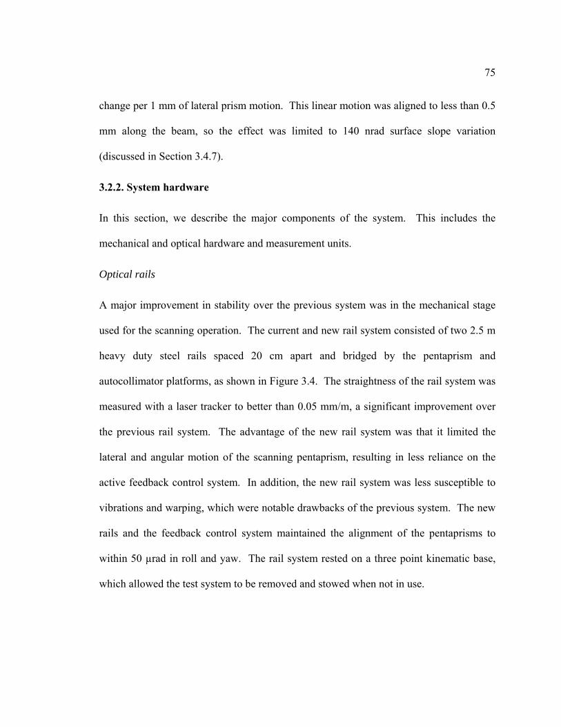
75

change per 1 mm of lateral prism motion. This linear motion was aligned to less than 0.5

mm along the beam, so the effect was limited to 140 nrad surface slope variation

(discussed in Section 3.4.7).

3.2.2. System hardware

In this section, we describe the major components of the system. This includes the

mechanical and optical hardware and measurement units.

Optical rails

A major improvement in stability over the previous system was in the mechanical stage

used for the scanning operation. The current and new rail system consisted of two 2.5 m

heavy duty steel rails spaced 20 cm apart and bridged by the pentaprism and

autocollimator platforms, as shown in Figure 3.4. The straightness of the rail system was

measured with a laser tracker to better than 0.05 mm/m, a significant improvement over

the previous rail system. The advantage of the new rail system was that it limited the

lateral and angular motion of the scanning pentaprism, resulting in less reliance on the

active feedback control system. In addition, the new rail system was less susceptible to

vibrations and warping, which were notable drawbacks of the previous system. The new

rails and the feedback control system maintained the alignment of the pentaprisms to

within 50 µrad in roll and yaw. The rail system rested on a three point kinematic base,

which allowed the test system to be removed and stowed when not in use.

76

FIGURE 3.4. Solid model of the scanning pentaprism rail system showing the mounting platforms and the three point kinematic base.

Autocollimators

We used two electronic autocollimators. The first was a high resolution autocollimator

(Elcomat 2000 made by Moller-Wedel [44]) used for the surface slope measurements.

The Elcomat 2000 provided a 40 mm collimated beam, which was projected onto the

mirror surface using the two pentaprisms (as described previously). The reflected beam

was detected by the Elcomat and angle deviations caused by slope variations in the mirror

surface were measured. The Elcomat also functioned as part of the active feedback

control system that monitored cross-scan motion due to prism roll and yaw motions.

The second autocollimator had less angular resolution (model 3700 made by

United Detector Technologies [45]). The UDT 3700 autocollimator was aligned to a

return flat mirror that was attached to the scanning pentaprism assembly (see Figure 3.1

Reference pentaprism platform

Scanning pentaprism platform

Heavy-duty steel rails

Three-point kinematic base

Scanning pentaprism assembly

Autocollimator system platform

77

or 3.5). The UDT autocollimator was the main component of the active feedback control

used to monitor the yaw motions of the scanning pentaprism. The UDT autocollimator

was insensitive to roll motion of the pentaprism, but the Elcomat sensed the line of sight

roll, which was caused by the combination of the prism roll and yaw motions. The prism

roll was determined as the difference between the line of sight roll and the prism yaw.

The UDT helped decouple the motions for the Elcomat. The feedback control then

maintained both the roll and yaw alignment of the scanning pentaprism to better than 50

µrad (see Section 3.4.2).

Pentaprisms and pentaprism mounts

The first (reference) pentaprism had a coupling wedge that allowed about 50%

transmission of the beam to the second (scanning) pentaprism, as shown schematically in

Figure 3.1. We estimated measuring through the reference prism with the wedge caused

about 50 nrad rms measurement error in the scanning mode (see Section 3.5.2).

The pentaprism holders provided secure mounts and remote adjustment of prism

yaw and roll through Pico-motor™ linear actuators (see Figure 3.5). The Pico-motor™

actuators were controlled through the feedback control system; any misalignments of

prisms were fixed with sending commands to the Pico-motors™ to drive the prisms back

into alignment. The prism assemblies were mounted on rail cars, which moved on the

two parallel steel rails.

78

FIGURE 3.5. Pentaprism assemblies integrated into the system. Electronically controlled shutters are located at the exit face of each prism. The autocollimator system (not shown) is mounted to the left.

Shutters

We used two electronically controlled shutters. The shutters were mounted between the

prisms and the test mirror, as shown in Figure 3.5. The shutters allowed alternating

measurements between the prisms. Shutter A was open and shutter B was closed when

measuring though the reference prism occurred. The shutter states were reversed when

measuring through the scanning prism occurred. A delay of a few seconds between

shutter operation and data acquisition allowed vibrations caused by the shutters to damp

out.

Scanning pentaprism assembly

Reference pentaprism assembly

Pico-motors

Shutters

Feedback mirror

79

Wedge plate for pentaprism apex angle error compensation

The reference pentaprism had a noticeable apex angle error. The beam deviation of this

pentaprism was 90° +ϕ, where ϕ is the additional beam deflection caused by the error in

the prism apex angle. A wedge plate was inserted at the output of the reference prism to

compensate for the additional beam deflection. We assumed the wedge plate introduced

negligible errors to the measurement.

3.2.3. System integration

The system can be thought of as an assembly of subsystems. The subsystems included

1. Autocollimator system,

2. Reference pentaprism assembly,

3. Scanning pentaprism assembly, and

4. Electronics including the workstation and software for the active feedback control.

The rail system is the foundation upon which these subsystems were integrated

(see Figure 3.5). Subsystems one through three were mounted on separate carriage

platforms. The platforms can slide on the rail tracks. Subsystems one and two were

locked into position at one end of the rails. The scanning pentaprism assembly, or

subsystem three, was allowed to translate over the rails. The electronics and cabling for

feedback control were housed in a breakout box and mounted underneath the

autocollimator system platform (not visible in Figure 3.6).

The fully integrated system is shown in Figure 3.6. The entire system can be

lifted with a hoist and positioned kinematically over the large mirror.

80

FIGURE 3.6. A fully integrated and operational scanning pentaprism test system. The vertical post next to the Elcomat was used to mount a He-Ne laser for the initial alignment of the system. Cabling attached to the pentaprism assemblies are used to control the Pico-motors™ through active feedback. The UDT beam is folded with a 50 mm mirror to the feedback mirror.

3.2.4. System alignment

The accurate alignment of the system, especially of the pentaprisms, is essential to slope

measurement accuracy [27-40]. The system alignment was performed in several steps

described below.

1) The large flat mirror rested on stable mechanical supports and a high performance

rotary air bearing table, which was initially leveled to gravity. The pentaprism rails were

also initially leveled to gravity, thus tilt between the test surface and the rails was

minimized from the beginning.

2) A standard He-Ne laser was mounted in place of the measuring autocollimator. The

laser was aligned to the rails by placing a crosshair target on the scanning pentaprism

assembly, then pointing the laser at the crosshair while sliding the penataprism assembly

ELCOMAT autocollimator

UDT autocollimator

Reference pentaprism

Scanning pentaprism

Feedback mirror

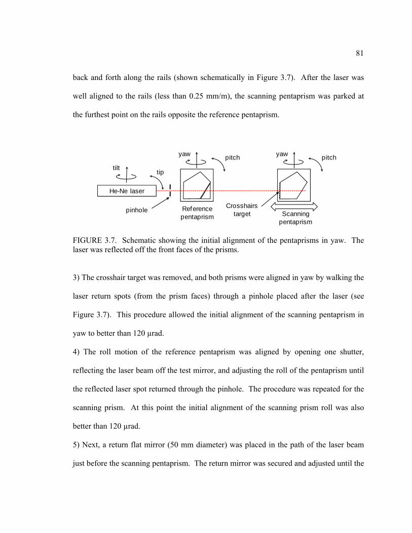
81

back and forth along the rails (shown schematically in Figure 3.7). After the laser was

well aligned to the rails (less than 0.25 mm/m), the scanning pentaprism was parked at

the furthest point on the rails opposite the reference pentaprism.

FIGURE 3.7. Schematic showing the initial alignment of the pentaprisms in yaw. The laser was reflected off the front faces of the prisms.

3) The crosshair target was removed, and both prisms were aligned in yaw by walking the

laser return spots (from the prism faces) through a pinhole placed after the laser (see

Figure 3.7). This procedure allowed the initial alignment of the scanning pentaprism in

yaw to better than 120 µrad.

4) The roll motion of the reference pentaprism was aligned by opening one shutter,

reflecting the laser beam off the test mirror, and adjusting the roll of the pentaprism until

the reflected laser spot returned through the pinhole. The procedure was repeated for the

scanning prism. At this point the initial alignment of the scanning prism roll was also

better than 120 µrad.

5) Next, a return flat mirror (50 mm diameter) was placed in the path of the laser beam

just before the scanning pentaprism. The return mirror was secured and adjusted until the

He-Ne laser

Scanning pentaprism


pitchyaw pitchyaw

tiptilt

Crosshairs targetpinhole

82

reflected laser beam returned through the pinhole. The laser and the pinhole were

removed, and the measuring autocollimator was put in place. The autocollimator was

aligned to the return mirror in both the horizontal and vertical axes. At this point the

autocollimator was aligned to the rails and the pentaprisms to better than 120 µrad.

6) The fine alignment was performed iteratively using the read-out of the autocollimator.

While the test surface remained fixed, adjustments were made to the autocollimator and

the pentaprisms. Table 3.1 lists the angular motions that affected the beam line of sight

pointing (pentaprism yaw and roll and autocollimator roll). These are the motions that

required alignment. First, the reference pentaprism was scanned in yaw by

approximately ±250 µrad, and the autocollimator horizontal and vertical angle readings

were observed. The behavior of this motion is linear on the angle readings (vertical

versus horizontal angle) [31-33]. A finite slope in the angle readings indicated a

misalignment between the autocollimator and test surface in roll [33]. With the test

surface fixed, adjustment was made to the autocollimator to minimize this misalignment.

After adjusting the roll of the autocollimator, the prism was re-scanned in yaw. Roll of

the autocollimator was aligned when the angle readings were no longer coupled for the

prism yaw scan. The procedure was repeated for the scanning prism. The autocollimator

roll was now aligned to better than 50 µrad.

7) Next, the reference prism was scanned in roll by approximately ±250 µrad, and the

autocollimator horizontal and vertical angle readings were observed. The behavior of

this motion is quadratic on the angle readings (vertical versus horizontal angle) [31-33].

Any coupled readings indicated a misalignment of the prism in yaw. Yaw of the prism

83

was adjusted, and the prism was then re-scanned in roll. The prism yaw was aligned

when no noticeable coupling remained between the angle readings during the roll scans.

At this point, the roll motion was constrained to the vicinity of the quadratic minimum

[33]. This procedure was repeated for the scanning prism. Yaw and roll for both prisms

were now aligned to better than 50 µrad. At this point, the system was aligned and ready

to use.

3.3. System Performance

The scanning pentaprism system can be used in two modes: scanning and staring (non-

scanning). Diagonal surface scans were performed in the scanning mode (see Figure

3.8). In the staring mode, circumferential scans were performed where both prisms

remained fixed and the test flat rotated continuously while data was acquired (see Figure

3.12).

3.3.1. Diagonal line scans: scanning mode

In the scanning mode, the reference prism remained fixed and the scanning prism was

scanned across the diameter of the mirror. A diagram of three scan paths is shown in

Figure 3.8. This was achieved by rotating the test flat to two other positions after the first

scan. Using these three scans measured most of the low order aberrations [46]. The

results of three line scans are not presented here, but a similar measurement with

electronic levels was given and analyzed in Chapter two.

84

FIGURE 3.8. Schematic showing three line scans with the scanning pentaprism. This example shows the mirror being rotated in 120° steps for each scan.

A single diagonal scan measures only rotationally symmetric aberrations, as

presented in Chapter two. Figure 3.9 shows the result of a single diagonal scan on the

finished 1.6 m flat mirror. The results from the interferometer measurements showed that

the surface contained mainly symmetric errors (see Figure 3.11). Power was the main

surface error of interest, so only a single line scan was performed. Forward and

backward scans were performed for the same diagonal line, and the data were averaged.

Only the slope functions derived from the symmetric Zernike polynomials were fit to the

slope data. The linear component of the polynomial fit to the slope data then revealed

power in the flat mirror surface. This measurement yielded 11 nm rms in power.

B A

Large f lat mirror

Rotate af ter each scan

Three scan lines af ter two 120˚ rotations

of the test mirror

85

FIGURE 3.9. Surface slope measurements with the scanning pentaprism system and a low order polynomial fit. A linear component of the polynomial fit to the slope data gives information on power in the surface (11 nm rms).

Comparison to interferometric data

A radially normalized plot showing the scanning pentaprism slope data in comparison to

the Fizeau interferometer data for the 1.6 m test flat is shown in Figure 3.10. The figure

shows that the scanning pentaprism data and interferometer data, first differentiated to

obtain the surface slope, have no significant differences, except at the very edge where

high slopes were observed. The rms difference is about 160 nrad after removing the edge

point, which is within the accuracy (given in Section 3.4) of the scanning pentaprism test

in the scanning mode. The large Fizeau interferometer cannot measure power, so the

interferometer data was adjusted for power before the comparison. The description of the

large Fizeau interferometer is given in Chapter four.

86

FIGURE 3.10. Comparison of the scanning pentaprism and the interferometer data. The interferometer data was first diffentiated to get surface slope.

FIGURE 3.11. Fizeau interferometer measurement on the 1.6 m flat mirror.

57 nm PV12 nm RMS

(nm)

87

The Fizeau interferometer used a 1 m custom reference flat and subaperture

testing to measure the 1.6 m flat mirror [47]. The surface map, shown in Figure 3.11, is

on the finished mirror after combining the subaperture measurements.

3.3.2. Circumferential scans: staring mode

The circumferential scans provided information on aberrations that have θ dependence

such as astigmatism (2θ) and trefoil (3θ). Tilt between the autocollimator and the test

surface has a 1θ dependence. The main aberration measured in this mode was

astigmatism.

In the circumferential scans, both pentaprisms were fixed and the flat mirror was

continuously rotated (see Figure 3.12). The slope data were continuously acquired for

several full rotations of the flat mirror. The data were then averaged.

FIGURE 3.12. Circumferential scans, where both prisms were fixed and the mirror was continuously rotated, measured astigmatism and other θ dependent aberrations in the mirror surface.

B A

Large f lat mirror

Continuously rotate the mirror; both prisms are

f ixed

88

For the scans shown in Figure 3.13a, the reference pentaprism (B) was parked

near the edge of the large flat mirror, and the scanning pentaprism (A) was parked at the

center of the mirror. These measurements were performed while the mirror was in

production. The difference between the scans (Figure 3.13b) reveals the amount of

contributions of low order aberrations with θ dependence (dominated by tilt).

FIGURE 3.13. Circumferential scans at the center and edge of the large flat mirror (a), and difference in the scans and fit (b). The error bars in the scans indicate good stability of the rotary air bearing table.

A least squares fit of the difference data was performed using a fitting function of

the form

( ) ( ) ( ) ( )θθθθ 2cos2sincossin 22110 babaaf ++++= (3.3)

( ) ( )θθ 3cos3sin 33 ba ++ .

89

Table 3.2 lists the aberrations with θ dependence and their coefficient values after

the fit. The last column shows the equivalent surface error for each θ dependent

aberration.

TABLE 3.2. Aberrations with θ dependence measured with circumferential scans, fit coefficients and equivalent low order surface error.

Aberration term Fit function term(s) Fit coefficients

(μrad)

Equivalent low order surface

error

Piston 0a 0.0294 ---

Tilt ( ) ( )θθ cossin 11 ba + 0.6328, -1.2888 359 nm rms

Astigmatism ( ) ( )θθ 2cos2sin 22 ba + 0.0366, -0.0043 15 nm rms

Trefoil ( ) ( )θθ 3cos3sin 33 ba + 0.0993, -0.0283 18 nm rms

3.4. Error Analysis

3.4.1. Errors to line of sight beam motion

There were several error sources that contributed to the line of sight beam pitch (or in-

scan) motion. Below we describe the sources and quantify their effect on the beam line

of sight.

90

3.4.2. Errors from angular motions of the pentaprisms, autocollimator and test surface

Taking the second order terms listed in Table 3.1, an expression for the change in the in-

scan line of sight due to misalignments and angular motions of the pentaprism,

autocollimator, and test surface can be derived as:

( ) ( )TSPPPPACTSPPPPACPPPPLOS 2 γβγγγβγγγγα Δ+Δ+Δ+++Δ+Δ⋅=Δ (3.4)

( ) ( )PPPPTSPPPPTS βγγβγγ Δ+Δ++Δ+ ,

where each Δ term indicates the variation in prism, autocollimator, and test surface

motion for that angle. Equation 3.4 shows motions of the three components coupling

with misalignments to cause second order errors. Table 3.3 shows a summary of the

error terms that coupled into the measurement in the in-scan direction, and Table 3.4

shows the amount of contribution from each error term in Equation 3.4.

TABLE 3.3. Budget for alignment errors for the scanning pentaprism system.

Parameter Description Tolerance

γPP Initial misalignment of the prism roll < 0.13 mrad

ΔγPP Variation in prism roll < 0.05 mrad rms

γAC Misalignment of the autocollimator roll relative to direction of motion < 0.10 mrad

ΔγAC Variation in autocollimator roll < 0.05 mrad rms

βPP Initial misalignment of the prism yaw < 0.13 mrad

ΔβPP Variation in prism yaw < 0.05 mrad rms

γTS Misalignment of the test surface roll relative to the direction of motion < 0.10 mrad

ΔγTS Variation in test surface roll < 0.01 mrad rms

91

TABLE 3.4. Misalignment and perturbation influences on the in-scan line of sight.

Contribution (terms from Eq. 3.4)

Amount of line of sight deviation (nrad rms)

2γPP × ΔγPP 13

ΔγAC × γPP 7

ΔγAC × βPP 7

ΔγAC × γTS 5

γAC × ΔγPP 5

γAC × ΔβPP 5

γAC × ΔγTS 1

ΔγTS × γPP 1

ΔγTS × βPP 1

γTS × ΔγPP 5

γTS × ΔβPP 5

Root sum square 20

3.4.3. Mapping error

The slope errors in the polished test surface were expected to be less than 2 nrad/mm rms.

The position of the scanning prism (or the beam) on the test surface was known to better

than 2 mm. The error due to the scanning prism position, thus, contributed about 4 nrad

rms to the total error.

3.4.4. Thermal errors

The pentaprisms were made from BK7, which is fairly sensitive to temperature gradients

(7.1 x 10-6/°C). A linear temperature gradient in the prisms changes the index gradient

and prism geometry. The thermal analysis showed that a temperature gradient of

92

0.01°C/meter in the pentaprisms would cause an additional beam deflection in the line of

sight direction of 17 nrad [48]. The test system was used in scanning and staring modes

(see Section 3.3). The time scale for the modes of operation was relatively short

compared to the pentaprism’s thermal time constant. In the scanning mode we estimated

a single scan took one hour. For a full measurement, three scans were performed that

required about three hours to complete. In the staring mode, a measurement typically

took 10 to 15 minutes. Only the variation in temperature gradients during the 3 hour scan

in scanning mode and 10 to 15 minute scan in staring mode contributed to the line of

sight errors. The top level error budget allowed for change in the thermal gradient of

±0.04°C/meter for the scanning case and ±0.02°C/meter for the staring case. We then

expected a line of sight error of up to 34 nrad rms and 17 nrad rms for scanning and

staring cases, respectively.

3.4.5. Combined random errors

Table 3.5 shows the random errors for the pentaprism staring and scanning modes

separately. There was an additional error in acquiring the measurements from the

scanning pentaprism through the fixed pentaprism. This effect is included directly in

Table 3.5.

93

TABLE 3.5. Pentaprism test system independent measurement errors assumed to be uncorrelated.

Error description Staring mode (nrad

rms) Scanning mode (nrad

rms)

Autocollimator measurement uncertainty (range dependent)a 140 160

Prism and beam angle variation 20 20

Mapping error 4 4

Thermal effects 17 34

Effect of reference prism error 25 50

Coupling of lateral motion -- 80

Root sum square 145 190 a manufacturer’s specification.

3.4.6. Errors from coupling lateral motion of the pentaprisms

Phase or amplitude variations in the collimated beam did not affect the system

performance to first order, because these effects were common to both pentaprisms.

These variations, however, were coupled with lateral motion of the scanning prism

relative to the collimated beam. Similarly, beam errors coupled with lateral motion of the

scanning prism to cause second order errors. Coupling of phase errors, diffraction

effects, beam non-uniformity, and prism errors with lateral motion of the pentaprisms for

the scanning system was analyzed by Mallik et al [27-28]. This analysis for our system is

not repeated here; our system had better control of the lateral motion of the pentaprisms.

The lateral motion of the scanning prism in our system was aligned and maintained to 0.5

mm. The combined effect of these errors was then estimated to be 80 nrad rms.

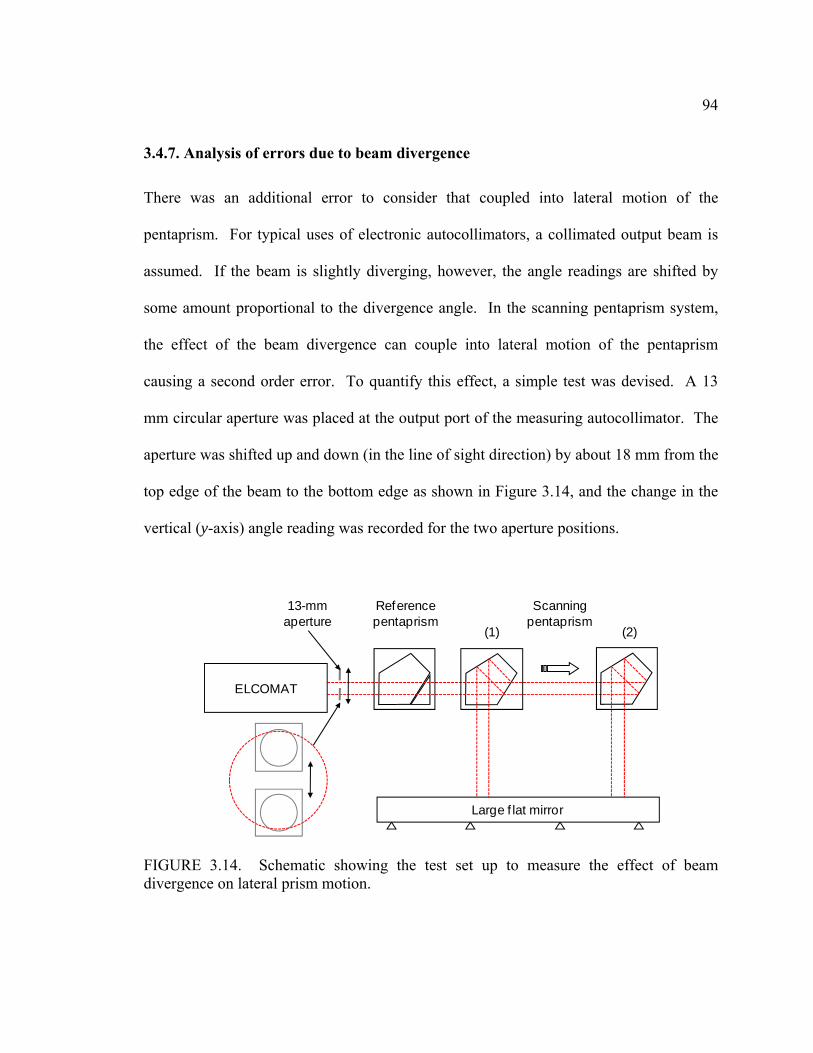
94

3.4.7. Analysis of errors due to beam divergence

There was an additional error to consider that coupled into lateral motion of the

pentaprism. For typical uses of electronic autocollimators, a collimated output beam is

assumed. If the beam is slightly diverging, however, the angle readings are shifted by

some amount proportional to the divergence angle. In the scanning pentaprism system,

the effect of the beam divergence can couple into lateral motion of the pentaprism

causing a second order error. To quantify this effect, a simple test was devised. A 13

mm circular aperture was placed at the output port of the measuring autocollimator. The

aperture was shifted up and down (in the line of sight direction) by about 18 mm from the

top edge of the beam to the bottom edge as shown in Figure 3.14, and the change in the

vertical (y-axis) angle reading was recorded for the two aperture positions.

FIGURE 3.14. Schematic showing the test set up to measure the effect of beam divergence on lateral prism motion.

ELCOMAT

Scanning pentaprism


Large f lat mirror

(1) (2)

13-mm aperture

95

For the case when the scanning pentaprism was close to the reference prism (1),

the change in the autocollimator y-axis angle reading was about 10 µrad. The scanning

prism was then moved to the far edge of the flat mirror (2), and performed the aperture

shifts. For this case, the change in the y-axis angle reading was about 15 µrad. From

these measurements we can estimate that this effect caused 280 nrad slope change per 1

mm of lateral motion. The pentaprism linear motion was aligned to less than 0.5 mm

along the beam, so the effect is limited to 140 nrad surface slope variation. This

systematic slope variation of ±70 nrad corresponds to surface power of less than 8 nm

rms.

3.4.8. Monte Carlo analysis of system performance

A Monte Carlo simulation on the three diagonal surface scans separated by 120° was

performed to determine the uncertainty distributions of the low order Zernike aberrations

using a noise of 0.3 µrad rms for a single differential measurement. This analysis

assumed 42 measurement points per scan. From the simulation the measurement

uncertainty of each of the low order aberrations can be estimated as shown in Table 3.6.

The simulation result in Table 3.6 shows that a 2 m flat mirror can be measured to 14 nm

rms of low order aberrations with the scanning pentaprism system after careful system

alignment. The measurement of power has 8 nm rms due to the systematic effect listed

above, limiting the surface power measurement to 9 nm rms.

96

TABLE 3.6. Scanning pentaprism measurement uncertainty for the low order Zernike aberrations assuming 0.3 µrad rms noise for a single differential measurement, three line scans, and 42 measurement points per scan.

Zernike aberration Measurement accuracy

(nm rms)

Power 9

Cos Astigmatism 8

Sin Astigmatism 8

Cos Coma 4

Sin Coma 4

Spherical 2

Secondary Spherical 2

Root sum square 16

3.4.9. Monte Carlo analysis of sensitivity to noise and number of measurement points per scan

Figures 3.15 through 3.17 show additional results of Monte Carlo simulations of the

sensitivities of the low order Zernike aberrations to noise and the number of

measurements points per scan. The analysis assumes three diagonal line scans (separated

by 120°) across a 2 m flat mirror and measurement noise normalized to 1 µrad rms. The

measurement spacing was varied for each number of measurement points to get a

distribution of the measurement uncertainty.

The sensitivities should get better as N1 , where N is the number of measurement

points per scan. An equation of the form

2/1−= ANε (3.5)

97

was, therefore, fitted to the data points, where ε is the measurement uncertainty and A is

the sensitivity to noise. The coefficient A was determined that allowed that best fit

through the data points. In addition to verifying the N1 effect on the measurement

uncertainty, the analysis also shows that the sensitivities of the aberrations depend on the

how the measurement points are distributed across the mirror diameter. For example,

varying the sample spacing of the five measurement point across the mirror gives a

distribution of the uncertainty values, as seen in the proceeding plots.

TABLE 3.7. Summary of the values of the sensitivity to noise for the proceeding plots (Figures 15 through 17).

Power (Z4)

Cos Astigmatism

(Z5)

Sin Astigmatism

(Z6) Cos Coma

(Z7) Sin Coma

(Z8) Spherical

(Z9)

A 110 185 180 84 84 56

98

1

10

100

1 10 100 1000

Measuremen

t uncertainty (nm

rms)

Number of measurement points per scan

Power (Z4) sensitivity

1

10

100

1 10 100 1000

Measuremen

t uncertainty (nm

rms)


Spherical (Z9) sensitivity

FIGURE 3.15. Power (Z4) and spherical aberration (Z9) sensitivity to noise and number of measurement points per scan. Three line scans (separated by 120˚) on a 2 m flat mirror and 1 µrad rms noise were assumed. A = 110 for power and A = 56 for spherical aberration.

99

1

10

100

1 10 100 1000

Measuremen

t uncertainty (nm

rms)


Cos Astigmatism (Z5) sensitivity

1

10

100

1 10 100 1000

Measuremen

t uncertainty (nm

rms)


Sin Astigmatism (Z6) sensitivity

FIGURE 3.16. Astigmatism (Z5, Z6) sensitivity to noise and number of measurement points per scan. Three line scans (separated by 120˚) on a 2 m flat mirror and 1 µrad rms noise were assumed. A = 185 for cos astigmatism and A = 180 for sin astigmatism.

100

1

10

100

1 10 100 1000

Measuremen

t uncertainty (nm

rms)


Cos Coma (Z7) sensitivity

1

10

100

1 10 100 1000

Measuremen

t uncertainty (nm

rms)


Sin Coma (Z8) sensitivity

FIGURE 3.17. Coma (Z7, Z8) sensitivity to noise and number of measurement points per scan. Three line scans (separated by 120˚) on a 2 m flat mirror and 1 µrad rms noise were assumed. A = 84 for both components of coma.

101

TABLE 3.8. Definition of mid order Zernike (UofA) polynomials. The angle, θ, is measured counter clockwise from the x-axis, and the radial coordinate is the normalized dimensionless parameter, ρ.

Zernike term Polynomial, Z(ρ,θ) rms

Z10 – cos trefoil 8 ρ3 cos 3θ

Z11 – sin trefoil 8 ρ3 sin 3θ

Z12 – cos secondary astigmatism 10 (4ρ2 – 3)ρ2 cos 2θ

Z13 – sin secondary astigmatism 10 (4ρ2 – 3)ρ2 sin 2θ

Z14 – cos secondary coma 12 (10ρ4 – 12ρ2 + 3)ρ cos θ

Z15 – sin secondary coma 12 (10ρ4 – 12ρ2 + 3)ρ sin θ

Z16 – secondary spherical 7 (20ρ6 – 30ρ4 + 12ρ2 – 1)

Z17 – cos pentafoil 10 ρ4 cos 4θ

Z18 – sin pentafoil 10 ρ4 sin 4θ

Z25 – tertiary spherical 9 70ρ8 – 140ρ6 + 90ρ4 – 20ρ2 + 1

3.4.10. Monte Carlo analysis of noise coupling into mid order Zernike aberrations for number of line scans and number of measurement points per scan

The analysis in this section looks at measurement noise normalized to 1 µrad rms

coupling into mid order Zernike aberrations (defined in Table 3.8) for the number of line

scans and number of measurement points per scan on a 2 m diameter flat mirror. The line

scans are equally spaced in angle (as shown in Figure 2.6) and the measurement points

per scan are equally spaced across the diameter of the mirror. The proceeding plots

shown are for the case of three line scans separated by 120° going through the center of

the mirror. More plots are available in the appendix for line scans that are offset from the

center of the mirror.

102

Summary of the proceeding plots (Figures 18 through 20):

1. The analysis assumes measurement noise normalized to 1 μrad rms coupling into mid

order Zernike aberrations for a 2 m flat.

2. The sensitivity to trefoil requires four line scans, and the sensitivity to pentafoil (4θ)

requires five line scans. The proceeding plots are for the case of three line scans only,

so trefoil and pentafoil are omitted. The results for more lines scans are provided in

the appendix.

3. The effect of increasing the number of measurement points generally reduces the

measurement coupling into mid order Zernike aberrations by mAN − , where A would

be the sensitivity to noise and a constant, N is the number of measurement points, and

m is the power with an ideal value of 0.5.

4. The plots were fitted with the function 5.0−AN . The coefficient A was chosen that

allowed a best fit to the distribution of data points. The distribution of the data for

each number of measurement points comes from varying the sampling spacing. For

small N, the plots deviated from the fitting function due to under sampling of the

aberration. The points where the deviations occur are labeled Nmin, a transition point

for under sampling to full sampling.

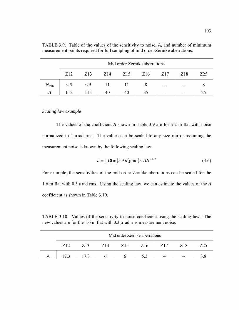
103

TABLE 3.9. Table of the values of the sensitivity to noise, A, and number of minimum measurement points required for full sampling of mid order Zernike aberrations.

Mid order Zernike aberrations

Z12 Z13 Z14 Z15 Z16 Z17 Z18 Z25

Nmin < 5 < 5 11 11 8 -- -- 8

A 115 115 40 40 35 -- -- 25

Scaling law example

The values of the coefficient A shown in Table 3.9 are for a 2 m flat with noise

normalized to 1 μrad rms. The values can be scaled to any size mirror assuming the

measurement noise is known by the following scaling law:

( ) ( ) 2/121 μradm −×Δ×= AND θε (3.6)

For example, the sensitivities of the mid order Zernike aberrations can be scaled for the

1.6 m flat with 0.3 μrad rms. Using the scaling law, we can estimate the values of the A

coefficient as shown in Table 3.10.

TABLE 3.10. Values of the sensitivity to noise coefficient using the scaling law. The new values are for the 1.6 m flat with 0.3 μrad rms measurement noise. Mid order Zernike aberrations

Z12 Z13 Z14 Z15 Z16 Z17 Z18 Z25

A 17.3 17.3 6 6 5.3 -- -- 3.8

104

1

10

100

1 10 100 1000Measuremen

t error (nm rms)


Cos secondary astigmatism (Z12) sensitivity

1

10

100


t error (nm rms)


Sin secondary astigmatism (Z13) sensitivity

FIGURE 3.18. Measurement noise normalized to 1 µrad rms coupling into secondary astigmatism (Z12, Z13) for number of line scans and number of measurement points over a 2 m flat. A = 115 for both components of astigmatism.

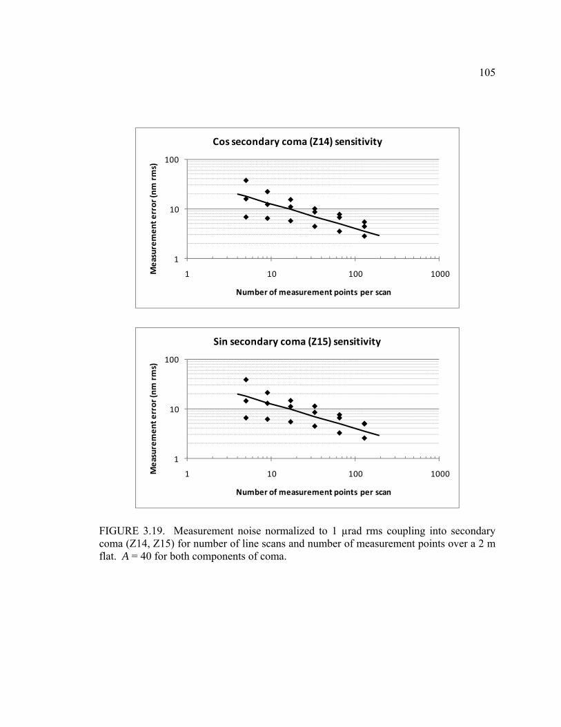
105

1

10

100


t error (nm rms)


Cos secondary coma (Z14) sensitivity

1

10

100


t error (nm rms)


Sin secondary coma (Z15) sensitivity

FIGURE 3.19. Measurement noise normalized to 1 µrad rms coupling into secondary coma (Z14, Z15) for number of line scans and number of measurement points over a 2 m flat. A = 40 for both components of coma.

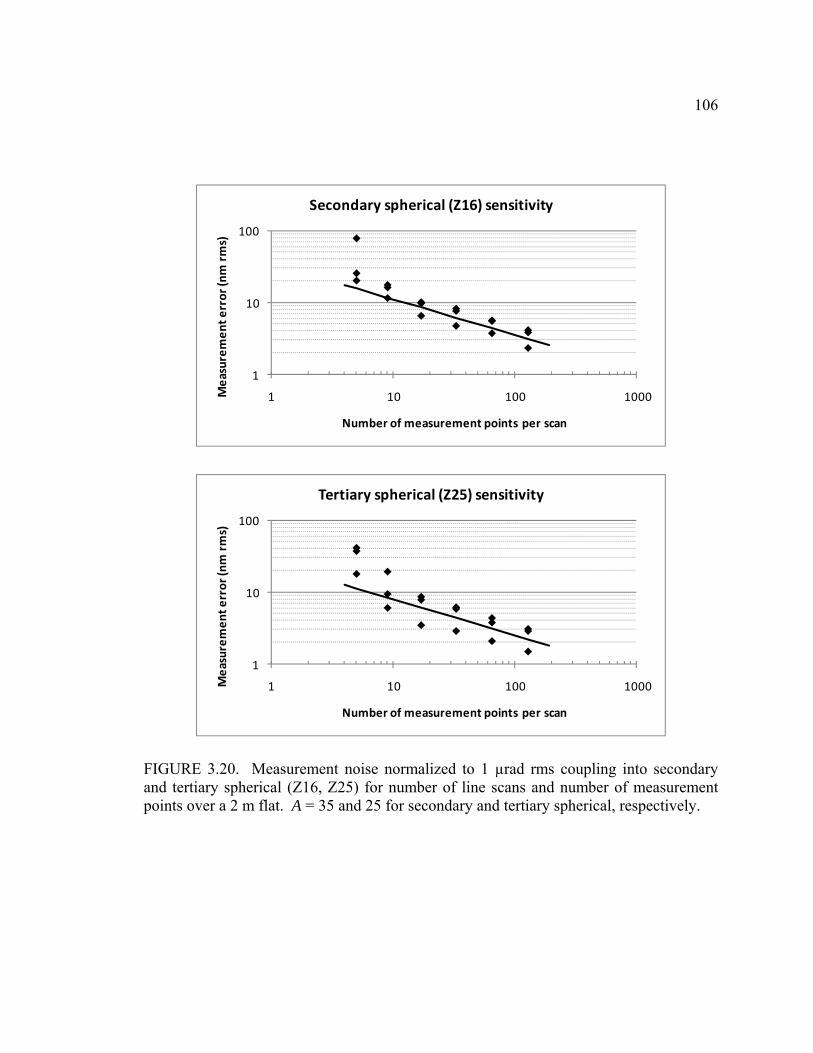
106

1

10

100


t error (nm rms)


Secondary spherical (Z16) sensitivity

1

10

100


t error (nm rms)


Tertiary spherical (Z25) sensitivity

FIGURE 3.20. Measurement noise normalized to 1 µrad rms coupling into secondary and tertiary spherical (Z16, Z25) for number of line scans and number of measurement points over a 2 m flat. A = 35 and 25 for secondary and tertiary spherical, respectively.

107

3.4.11. Effect of sampling spacing and noise on measurement error

The measurement sampling arrangement and noise affects the measurement uncertainty,

especially for higher order Zernike aberrations. The previous set of plots showed a

distribution of data points for each number of measurement points per scan. This can be

explained by varying the sampling spacing. In Figure 3.21 we show two different

sampling arrangements for five measurement points across the mirror and a fit to the

point using the slope function for secondary spherical. The five measurement points,

showing some noise variation, in both cases are distributed evenly across the mirror (the

plot is normalized in radius). In one case (square markers) the edges of the mirror are

sampled. In the other case (triangle markers) the edges are not sampled, but the sample

spacing is smaller.

‐60

‐40

‐20

0

20

40

60

‐1 ‐0.8 ‐0.6 ‐0.4 ‐0.2 0 0.2 0.4 0.6 0.8 1

slope

radius (normalized)

Gradient of Secondary Spherical (Z16)

FIGURE 3.21. Sampling for secondary spherical aberration (Z16) with two different five equally spaced sample points (sample points are showing noise variation).

108

In the case of sampling at the edges the measurement error is better controlled,

because the edge points alone limit the amount of variation in the fit. For the other case

there is no constraint at the edges, so the measurement error is not well controlled and has

more variation. The latter case then is not a recommended sampling arrangement due to

larger measurement error, especially for higher order Zernike aberrations.

3.4.12. Limitation of the Zernike basis set

The fits to the slope data were performed using a Zernike basis. The results of the

Monte Carlo analysis and the example given in Section 3.4.11 showed the polynomials

with this basis seemed to become unbalanced in slope space, because in slope space the

gradients of the Zernike polynomials were used for the least squares fitting. More weight

is given to the higher polynomial orders; therefore, behavior at the edges varies more

rapidly than around the center of the mirror. Perhaps it would be better to develop and

use another orthogonal basis set of polynomials that is more balanced in slope space to

perform the least squares fitting. After the surface has been reconstructed with the new

orthogonal polynomials, the surface can then be related back to Zernike polynomials.

3.5. Conclusion and Future Work

We provided an analysis of the scanning pentaprism system that measured flatness in

large flat mirrors with an option to measure other low to mid order aberrations and only θ

dependent aberrations. The system alignment was discussed in detail. The measurement

accuracy was limited by second order influences from misalignments and autocollimator,

pentaprism, and test surface motions, which were minimized through careful system

109

alignment and active pentaprism motion control. A Monte Carlo simulation of the

system performance was performed based on the measurement uncertainty estimated

from the error analysis. The simulation result showed the uncertainty in the measured

low order Zernike aberrations and measurements to about 15 nm rms of low-order

aberrations are achievable for 2 m class flat mirrors. Additional Monte Carlo analysis

was performed that studied the effect of measurement noise coupling into mid order

Zernike aberrations for the number of line scans and number of measurement points per

scan over a 2 m flat mirror.

The high accuracy of the test system makes it ideal for absolute testing of

arbitrarily large flat mirrors. This test can be used as a final test on the surface figure or

to guide polishing during fabrication. The kinematic base allows the test system to be

moved to the polishing table without moving the test flat to a testing fixture and stowed

when not in use or during polishing.

The results were obtained using the Zernike basis for polynomials. These

polynomials seemed to become unbalanced in slope space. A different orthogonal basis

set of polynomials might work better for the least squares fitting in slope space. This

investigation is left open for future work.

Absolute calibration of the system was not performed. This can be accomplished

using liquid reference surfaces over very long test paths (~4 m), where the liquid surfaces

are only limited by the curvature of the earth (sag/power = 0.31 µm peak to valley over 4

m). The result will be excellent characterization of the system performance. This task

was left open for future work.

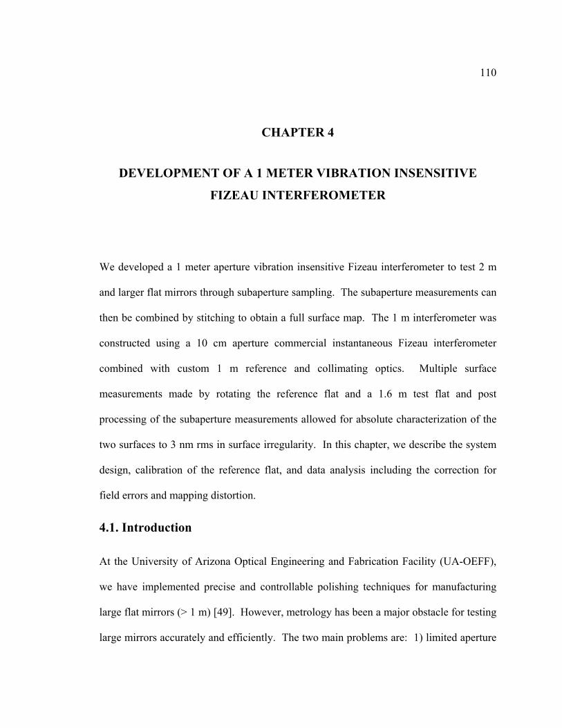
110

CHAPTER 4

DEVELOPMENT OF A 1 METER VIBRATION INSENSITIVE

FIZEAU INTERFEROMETER

We developed a 1 meter aperture vibration insensitive Fizeau interferometer to test 2 m

and larger flat mirrors through subaperture sampling. The subaperture measurements can

then be combined by stitching to obtain a full surface map. The 1 m interferometer was

constructed using a 10 cm aperture commercial instantaneous Fizeau interferometer

combined with custom 1 m reference and collimating optics. Multiple surface

measurements made by rotating the reference flat and a 1.6 m test flat and post

processing of the subaperture measurements allowed for absolute characterization of the

two surfaces to 3 nm rms in surface irregularity. In this chapter, we describe the system

design, calibration of the reference flat, and data analysis including the correction for

field errors and mapping distortion.

4.1. Introduction

At the University of Arizona Optical Engineering and Fabrication Facility (UA-OEFF),

we have implemented precise and controllable polishing techniques for manufacturing

large flat mirrors (> 1 m) [49]. However, metrology has been a major obstacle for testing

large mirrors accurately and efficiently. The two main problems are: 1) limited aperture

111

sizes of commercial interferometers, and 2) stitching is required but limits the

measurement accuracy and efficiency.

To enable surface testing of 2 m class and larger flat mirrors, we scaled up a 10

cm aperture instantaneous Fizeau interferometer to 1 m and performed subaperture

testing. We accomplished this by expanding the 10 cm beam to 1 m and inserting a 1 m

custom reference flat. The collimating optics were arranged such that the test was

performed vertically. The reference flat was held in a kinematic mount. The mount has a

three point base for mechanical stability and placement repeatability, and allowed six

equally spaced rotations of the reference flat. After multiple measurements and

measurement redundancy through rotations of the reference and the test flats, the

nonsymmetrical surface errors in the reference flat can be isolated from the test surface.

Power in the reference flat was calibrated using an auxiliary test system that measured

surface slopes very accurately [50]. The reference flat surface errors were then stored in

a reference data file, which was used to correct each of the subaperture measurements

before combining them.

4.1.1. Testing large flat mirrors

The most efficient and accurate method of measuring flat surfaces uses a Fizeau

interferometer with a flat reference surface. Most commercially available interferometers

are limited to 10 to 15 cm apertures, although 30 cm [51-52] and 60 cm [53] aperture

interferometers have been demonstrated. Large flat surfaces can be measured with small

aperture interferometers, but stitching subaperture data is required [17-20]. As the

112

subaperture becomes smaller compared to the size of the test mirror, the accuracy and

efficiency of the measurement diminishes.

Due to size limitations of commercial interferometers for direct measurements,

large flat mirrors are normally tested in a Ritchey-Common configuration [16, 21]. The

Ritchey-Common test, however, is limited in other areas as discussed in Chapter one.

In order to guide our polishing of high quality flat mirrors, the surface

measurements must be efficient to perform and provide accuracy of a few nanometers. It

is optimal to measure flat mirrors in situ as they rest on our 4 m polishing table, which

allows rapid turnaround between testing and polishing. It is impractical to isolate the

system from vibrations, but the test hardware must function in the shop environment,

which had considerable vibration and air currents.

The vibration insensitive Fizeau interferometer meets all of our requirements.

The 1 m reference surface can be held to a few centimeters above the mirror under test as

it rests on the polishing machine. The short air gap and the use of polarization for

instantaneous phase shifting give high accuracy in the presence of vibration and thermal

effects.

4.1.2. Instantaneous interferometry

Vibration is a major problem in optical testing. Industrial environments, such as optical

fabrication and testing facilities, are prone to vibrations and air motions. Vibrations are

especially problematic in large scale optical testing where the large optics and the

supporting mechanical structures are not easily isolated. In addition, air motions over

long test path lengths contribute to the overall fringe motion. In the presence of

113

vibrations, the standard phase shifting interferometry through temporal phase stepping is

inadequate for accurate optical testing. The time scale for mechanical vibrations is

shorter than the time between exposures. Thus, vibrations limit the ability to collect

accurate data. To overcome these problems, simultaneous acquisition of the phase

shifted frames is needed.

FIGURE 4.1. Schematic showing a Fizeau interferometer simultaneous phase shifting concept using polarizing element and orthogonal polarizations.

We use the Intellium H1000 (made by Engineering Synthesis Design, Inc. [54])

instantaneous Fizeau interferometer. This interferometer uses polarizing elements to

produce three simultaneous phase shifted signals for interference. In this method, two

orthogonal polarizations, A and B, are emitted by the interferometer, as shown in Figure

4.1. The polarizations can either be linear or circular. One polarization, B for example,

is reflected off the reference surface, and the other polarization, A, is reflected off the test

surface. The return signals are combined to produce a set of interference fringes

Decoding module

Reference surfaceWaveplate

Reference beam

Test beam

Polarizing beamsplitter

Test surface

114

simultaneously, which are then recorded by a decoding module. The interference fringes

are then combined to generate a phase map of the test surface.

4.2. Design and Analysis of the 1 Meter Fizeau Interferometer

A schematic of the 1 m Fizeau test system is shown in Figure 4.2. The inset photos are

the actual components of the ones shown schematically. The Intellium H1000

interferometer used a 30 mW laser diode at 657 nm as a source. The source emitted two

circularly polarized beams, as opposed to linearly polarized, to minimize birefringence

though the 1 m reference flat [55]. A standard reference diverger and the off axis

parabola (OAP) formed the beam expansion and collimation. The 1 m reference flat was

suspended over the large test surface (described in section 4.3.1).

4.2.1. Test concept

Fizeau interferometers require a collimated beam and a flat reference surface to test other

flat surfaces [15-16]. The Intellium H1000 emitted a 10 cm collimated beam. The

reference diverger and the OAP expanded the beam to 1 m. A 15 cm fold flat kept the

H1000 horizontally mounted and allowed the test to be done vertically.

In this arrangement of the interferometer, the probe beam was external to the

Intellium H1000 interferometer, hence the external reference surface. Interference

occurred between the reference flat bottom surface and test flat top surface. A small

wedge in the reference flat isolated the reflection off the top surface of the reference flat

from the measurements. The air gap between the reference and test surfaces was kept to

a few centimeters to minimize the errors from illumination. The 1 m beam then

115

subsampled the larger flat mirror under test. Rotating the large flat mirror underneath the

reference flat allowed for complete coverage of the flat mirror. The subaperture

measurements were corrected for errors. The corrected subaperture measurements were

then stitched together to obtain a full surface map.

FIGURE 4.2. Schematic of the 1 m Fizeau interferometer with an OAP for beam collimation and an external 1 m reference.

Large f lat miror

1 m reference f lat

H1000 Fizeau interferometer

Fold f lat

1 m illumination OAP

Rotary air bearing table

116

4.2.2. Test tower design

The test components shown in Figure 4.2 were integrated into a large test tower with base

dimensions 7.2 m × 3.3 m and height 4.2 m. The test tower was a four column weldment

with diagonally braced framework as shown in Figure 4.3. The columns were made out

of 12 mm thick 20 cm square metal tubes. The Intellium H1000 interferometer and the

fold flat were mounted on a platform. The platform was then suspended from the

horizontal cross member in the test tower. The test tower was braced at the top with two

additional brace beams, which held the OAP in place. The fully integrated structure is

shown in Figure 4.9. The entire structure was then moved over the polishing table. The

advantage of doing this was to allow the test flat to remain on the polishing table and

perform testing in situ. An additional horizontal cross member (not shown in the solid

model in Figure 4.3) was used as a place to stow the kinematic reference flat during

polishing. The tower was designed to vibrate below 15 Hz to ensure system stability.

Table 4.1 shows the three lowest vibration modes of the tower from the finite element

analysis (FEA) model.

TABLE 4.1. Fizeau test tower lowest frequency modes.

Frequency (Hz)

Mode Pinned ends Fixed ends

1 8.69 10.75

2 12.71 12.87

3 13.00 13.14

117

FIGURE 4.3. Solid (a) and FEA dynamic (b) models of the Fizeau test tower.

4.2.3. Collimation OAP design

The OAP was used as the beam collimator. The OAP was mounted in a whiffletree type

back support with tangential side supports as shown in Figure 4.4. The OAP was placed

in a downward looking orientation, tilted at 5.7° from vertical. The support allowed tip

and tilt adjustments for initial alignment and locking of the OAP.

118

FIGURE 4.4. OAP mounted in an 18 point whiffletree and band support. The mount provided tip and tilt adjustments.

FIGURE 4.5. FEA model of the mounted collimating OAP optical performance (5 nm rms).

OAP Back supports

Band support

24 nm PV5 nm RMS

(nm)852-1-4-7-10-13-16

119

Figure 4.5 shows the optical performance of the mounted OAP from the finite

element model. A maximum slope error of 0.1 µm/mm due to gravity and mount induced

surface deformation was derived from the system error budget. With this requirement,

the analysis predicted surface errors of 5 nm rms from gravity and the mount.

4.2.4. Field effect errors

The Intellium H1000 interferometer used two beams with orthogonal polarizations that

had a slight shear between them. If polarization A was used as the reference beam, then

polarization B must be the test beam for interference and phase shifting to occur. The

slight shear between the beams and using the OAP for beam collimation caused the

beams to traverse slightly different paths through the system. This effect of traversing

different path lengths caused field, or retrace, errors in the measurements [55]. To fix

this problem, measurements were taken with both polarizations as the reference beam and

the results were averaged to obtain a phase map that was free of field errors. Using

polarization B as a reference beam, however, resulted in inverted surface maps. This

inversion was verified with a simple but unambiguous test of introducing small tilts in

known directions and acquiring the surface data. The surface maps were re-inverted

before combining them with the measurements taken with polarization A as the reference

beam.

Figure 4.6 shows using both polarizations as reference beams to take surface

measurements and the average of the two measurements to eliminate the field errors.

This fix must be applied to each subaperture measurement before further data processing.

120

FIGURE 4.6. The 1 m Fizeau interferometer with polarization B as the reference beam (left), polarization A as the reference beam (center), and the average of the two measurements (right) to eliminate field errors.

The average surface map in Figure 4.6 exhibits trefoil, which is a result of the

three cable suspension of the reference flat (see Figure 4.7).

4.2.5. Wedge in test plate

There was a small wedge in the reference flat. The wedge allowed the reflection from the

back (top) surface of the reference flat to be isolated from the measurements. The wedge,

however, caused the beam spots from the A and B polarizations to be rotated and

translated at the image plane when the reference flat was rotated. Because of this, the

spots were tracked carefully to prevent errors in the measurements.

4.2.6. Distortion correction

Using the OAP to collimate the beam caused slight mapping errors. Mapping errors, also

known as distortion, occur when points on an object do not maintain their relative

spacing in the image plane. Distortion in each of the subaperture measurements must be

121

fixed before combining them to generate a full surface map. We developed a four-step

process to correct for distortion in each of the subaperture measurements.

1. First, we defined and fabricated a Mylar based film fiducial mask. A fiducial mask

contains a regular pattern of small circular apertures or fiducials. The mask is usually

placed at the test surface and that typically cover 5 to 10 pixels for easy locating in

the image plane. The physical spacing of the small apertures must be known. Our

mask contained 12 mm circular apertures spaced 10 cm apart.

2. Next, we imaged the fiducial mask through the system. This was accomplished by

placing the mask at the pupil, or the reference surface, and performing the normal

data acquisition.

3. Then, we defined fitting polynomials and determined their coefficients. This was

accomplished by relating the undistorted points in object space to the distorted

digitized points in image space through polynomials of degree n.

4. Finally, we filtered the distorted image through the fitting functions to generate an

image that was corrected for distortion.

The fitting polynomials were defined as

∑∑

=

=ji

ij

jiij

YXvy

YXux (4.1)

where x and y are the original image coordinates

X and Y are similar object coordinates

iju and ijv are coefficients to be determined through least squares fitting.

122

The degree of the polynomials, n = (i + j), determines the minimum number of

fiducial points required by the following formula,

( ) 1

23+

+≥

nnN . (4.2)

For example, a fitting polynomial of degree three requires a minimum of 10

fiducial points for correct determination of the coefficients

During testing we controlled the mapping to 2 mm, which coupled in as surface

error of about 1 nm rms.

4.3. System Integration

4.3.1. Reference flat and its mounting support

The reference flat was a 1 m transmissive fused silica polished to 100 nm peak to valley.

It was 11 cm thick and weighed about 195 kg. A mechanically stable kinematic mount

was designed to hold the reference flat, as shown in Figure 4.7. Three counter balanced

cables were attached to pucks carefully bonded to the top surface of the reference flat. In

addition, six tangential edge supports were added. The cables and the edge supports

offloaded about 60% of the reference flat weight (117 kg). As stated earlier, the three

cable suspension caused trefoil in the reference flat surface.

The kinematic base rested on three stable points. The three points were equally

spaced which allowed for three equally spaced rotations. Separately, a smaller top

support structure also rested on three points, which were offset by 60° from the base

points and allowed for three additional equally spaced rotations. Combined, the entire

123

support structure provided six equally spaced rotations and good position repeatability of

the reference flat.

The control of the gap between the reference and the test surfaces is important.

As the gap increases the accuracy of the test system degrades. For example, the test flat

may be assessed to an accuracy of 20 nm peak to valley. The illumination error was

expected to be less than 0.5 mrad. For this case, the gap between the reference and test

surfaces must be maintained to

2

1100 θλ

≤t ≈ 8 cm. (4.3)

FIGURE 4.7. Oblique top view of the kinematic support mount for the Fizeau reference flat. Cables, attached to the pucks, and a six point edge supports held the reference flat.

Bonded pucks and attached cables

Reference f lat

Kinematic base

Upper support

Test f lat Polishing

table

124

4.3.2. System alignment

To enable system alignment, each of the components in the test system required multiple

degrees of freedom with coarse and fine adjustments. The OAP mount provided

adjustments in tip and tilt. The reference flat mount provided coarse and fine adjustments

in tip and tilt. The fine adjustment was accomplished through three voltage driven piezo

transducer (PZT) stacks. The Intellium H1000 interferometer with the diverger and fold

flat was mounted on a stage with five degrees of freedom combining coarse and fine

adjustments. The system was first aligned as an autocollimation of the OAP with the

reference flat as the return flat. In this configuration, the diverger surface was the

reference surface and OAP surface was the test surface. During initial alignment, a pan

of oil was used as the return reference surface due to its natural alignment to gravity.

In the autocollimation test configuration, the OAP position was no longer in the

common path of the reference and the test beams, thus the OAP required adjustments to

get a minimum wavefront slope in the interference pattern. Most of the alignment error

introduced astigmatism. A combination of the OAP, H1000 interferometer and fold flat

iterative adjustments minimized the wavefront slope. The alignment of these components

was not critical, because all the surfaces before the reference surface are common path in

the Fizeau test. However, careful alignment was still performed to minimize any high

order effects. After the system alignment, we required the reference flat to be stable to 3

nm rms during testing.

To better understand the effects of OAP motion on the system alignment, the test

system was modeled as an autocollimation test using optical design software.

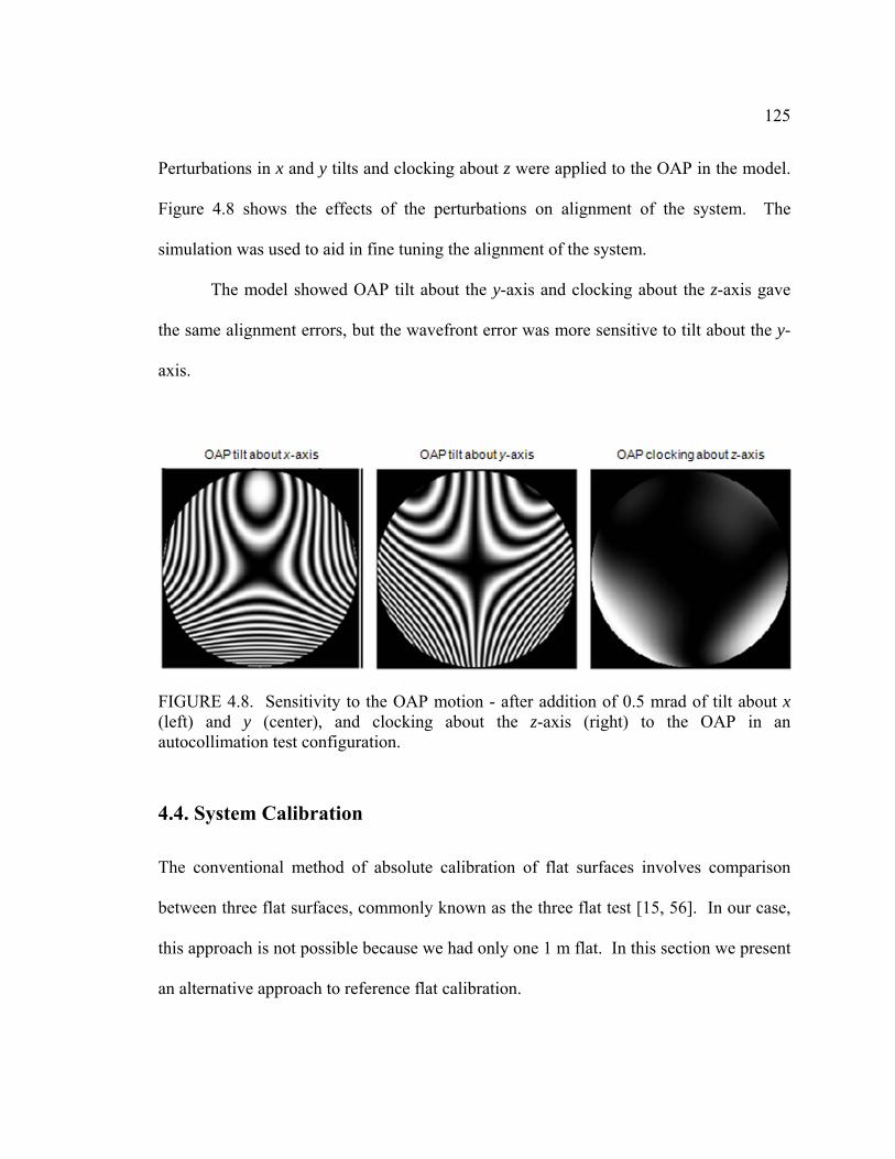
125

Perturbations in x and y tilts and clocking about z were applied to the OAP in the model.

Figure 4.8 shows the effects of the perturbations on alignment of the system. The

simulation was used to aid in fine tuning the alignment of the system.

The model showed OAP tilt about the y-axis and clocking about the z-axis gave

the same alignment errors, but the wavefront error was more sensitive to tilt about the y-

axis.

FIGURE 4.8. Sensitivity to the OAP motion - after addition of 0.5 mrad of tilt about x (left) and y (center), and clocking about the z-axis (right) to the OAP in an autocollimation test configuration.

4.4. System Calibration

The conventional method of absolute calibration of flat surfaces involves comparison

between three flat surfaces, commonly known as the three flat test [15, 56]. In our case,

this approach is not possible because we had only one 1 m flat. In this section we present

an alternative approach to reference flat calibration.

126

FIGURE 4.9. Solid model of the 1 m vibration insensitive Fizeau test system fully integrated and aligned.

4.4.1. Calibration of reference surface irregularity

By using overlapping subapertures along with multiple rotations of the reference and test

flats, we can obtain unbiased estimates of both the reference and the test surfaces [57-58].

The measurement algorithm that was used to obtain 24 subaperture measurements is

provided in Table 4.2. This procedure, shown schematically in Figure 4.10, helped in

separating the errors in the reference and test surfaces. Surface errors that moved with

the reference flat belonged to the reference flat; the remaining errors were associated with

the test flat. This method of rotating surfaces with no translations, however, was immune

Vibration-insensitive Fizeau interferometer

OAP

1 m reference f lat in kinematic mount

1.6 m test f lat

Polishing table on air bearings

Metal support structure

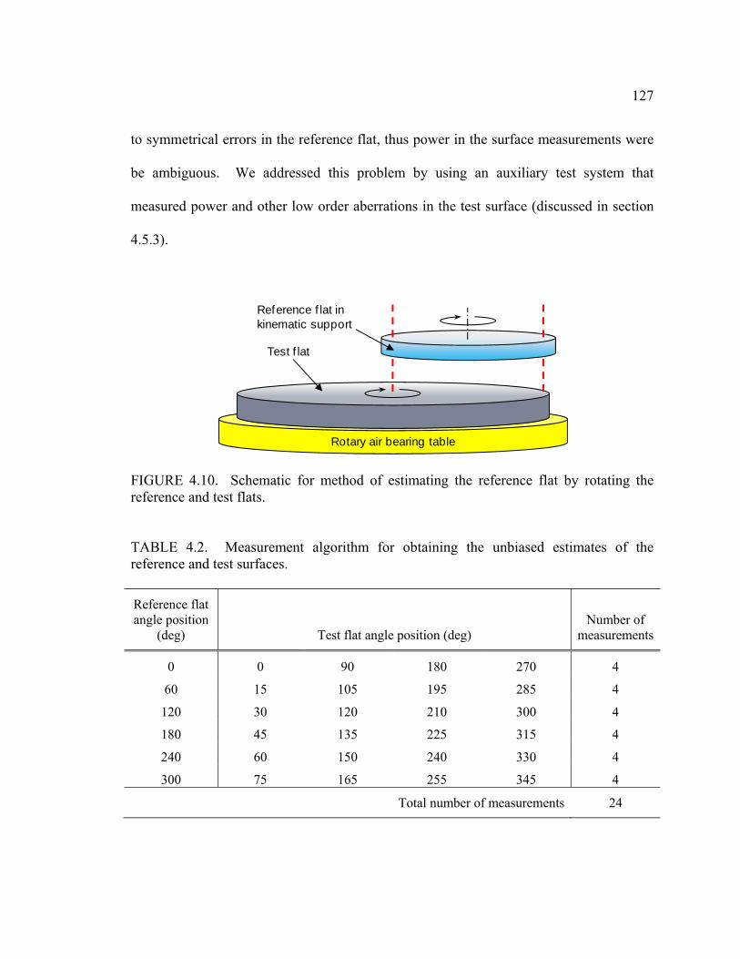
127

to symmetrical errors in the reference flat, thus power in the surface measurements were

be ambiguous. We addressed this problem by using an auxiliary test system that

measured power and other low order aberrations in the test surface (discussed in section

4.5.3).

FIGURE 4.10. Schematic for method of estimating the reference flat by rotating the reference and test flats.

TABLE 4.2. Measurement algorithm for obtaining the unbiased estimates of the reference and test surfaces. Reference flat angle position

(deg) Test flat angle position (deg) Number of

measurements

0 0 90 180 270 4

60 15 105 195 285 4

120 30 120 210 300 4

180 45 135 225 315 4

240 60 150 240 330 4

300 75 165 255 345 4

Total number of measurements 24

Test f lat

Rotary air bearing table

Reference f lat in kinematic support

128

An algorithm was developed that combined all the measurement data and

separated the surface errors in the reference and test surfaces using maximum likelihood

estimation [57-58]. Figure 4.11 shows the reference surface estimated after acquiring 24

subaperture measurements using the algorithm given in Table 4.2 and applying the

maximum likelihood estimation to separate the errors in the reference flat from the errors

in the test flat.

FIGURE 4.11. The 1 m reference surface estimated by modulation of the reference and test surfaces and performing maximum likelihood estimation. Multiple Zernikes terms were used to generate the surface (42 nm rms). The surface map shows the effect of the three point cable suspension.

The surface map shows 42 nm rms after removing ambiguous rotationally

symmetric errors. The surface map reveals the effect of the cable suspension as trefoil.

The positions of the three pucks bonded to the top surface are indicated by the three high

184 nm PV42 nm RMS

Reference Flat Surface Estimation by MLE (nm)

129

spots on the surface map. This surface map was saved as a reference data file. The file

was then be subtracted from each of the subaperture measurements before they are

combined. The error in the surface irregularity calibration was estimated to be 1 nm rms

[58].

4.4.2. Comparison to finite element analysis model

A simulation of optical performance was also performed on the finite element model of

the suspended reference flat. The simulation used the following parameters listed in

Table 4.3 for the mount shown in Figure 4.7.

TABLE. 4.3. The reference flat support parameters for the FEA model and simulation.

Six point edge whiffletree support Top surface cable support

• 60° puck spacing

• Pucks positioned at center of gravity plane of the reference flat

• Three pucks bonded to the top surface positioned at 28 cm from center (56% φ)

• 120° puck spacing

• 45° load wire angle

The result of the simulation is shown in Figure 4.12. The simulation output gave

29 nm rms, which is conservative compared to the result from the previous method

described above. The result from the simulation did not include errors such as

interferometer noise and illumination and alignment errors. Also the systematic errors

were not measured, and therefore were not included in the simulation. They were,

however, automatically included in the measured data, thus giving a higher rms surface

error for the reference flat shown in Figure 4.11.

130

FIGURE 4.12. Results of the FEA simulation on the mounted reference flat that shows the effects of the three cables suspension and edge supports.

4.4.3. Calibration of reference surface power

Power in the reference surface can come from two things: 1) power left in the surface

during polishing, and 2) power due to sag from gravity. Doing the multiple rotations of

the reference and test surfaces to obtain overlapping subapertures did not calibrate power

in the reference surface. An additional degree of freedom in translation of the reference

flat was needed to calibrate the symmetrical errors in the reference surface. This

additional degree of freedom was not available to us. Thus, power in the subaperture

measurements was ambiguous.

One method of measuring the reference surface power is to look at the cosine

effect at the reference surface [59]. With careful measurements of the slope errors and

the gap between the reference and test surfaces, we could quantify this effect, although

Reference Flat FEA Simulation

129 nm PV29 nm RMS

(nm) 7559432711-6-22-38-54

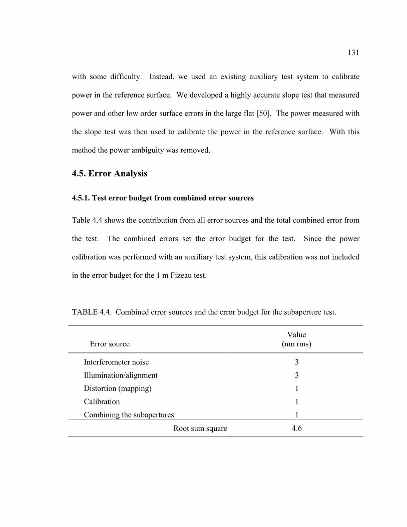
131

with some difficulty. Instead, we used an existing auxiliary test system to calibrate

power in the reference surface. We developed a highly accurate slope test that measured

power and other low order surface errors in the large flat [50]. The power measured with

the slope test was then used to calibrate the power in the reference surface. With this

method the power ambiguity was removed.

4.5. Error Analysis

4.5.1. Test error budget from combined error sources

Table 4.4 shows the contribution from all error sources and the total combined error from

the test. The combined errors set the error budget for the test. Since the power

calibration was performed with an auxiliary test system, this calibration was not included

in the error budget for the 1 m Fizeau test.

TABLE 4.4. Combined error sources and the error budget for the subaperture test.

Error source Value

(nm rms)

Interferometer noise 3

Illumination/alignment 3

Distortion (mapping) 1

Calibration 1

Combining the subapertures 1

Root sum square 4.6

132

4.6. Measurements on a 1.6 Meter Flat Mirror

Su [57-58] showed that the separation of the reference surface and test surface errors can

be accomplished to 3 nm rms using the maximum likelihood estimation method through

the repeatability of the subaperture measurements.

4.7. Conclusion

The developed 1 m vibration insensitive Fizeau interferometer has made accurate and

efficient testing of 2 m class and larger flat mirrors possible. The increased size in

aperture provided more surface coverage, thus less subaperture data to get full surface

coverage lead to less errors from stitching. Through overlapping subaperture

measurements and multiple rotations of the reference and test flats, errors from both

surfaces can be isolated by maximum likelihood estimation. An auxiliary test was used

to calibrate power in the reference flat. A reference data file containing errors from the

reference flat was generated and stored. This file was then subtracted from each

subaperture measurement before combining them. The results from the maximum

likelihood estimation showed that a 2 m mirror can be measured and the reference flat

calibrated to 3 nm rms. This Fizeau is an in situ test and can be used as a final test on the

surface figure or to guide polishing and figuring during fabrication. The kinematic mount

allows the reference flat to be moved and stowed during polishing.

133

SECTION II

ADVANCED FABRICATION TECHNOLOGIES

This second section contains a chapter on the methodology for manufacturing high

performance large flat mirrors with greater emphasis on the fabrication techniques that

we implemented. We found classical fabrication methods alone do not enable the

manufacture of quality large flat mirrors, because the classical methods are not scalable.

We introduced computer controlled polishing that used simulation software combined

with accurate and efficient metrology to achieve rapid convergence of polishing and

produce the best 1.6 meter flat mirror in the world (11 nm rms power and 6 nm rms

surface irregularity). This methodology used to produce the 1.6 meter flat can be

extended to 4 meters or larger flat mirrors, a key advantage over classical fabrication

methods.

134

CHAPTER 5

METHODOLOGY FOR FABRICATING AND TESTING LARGE

HIGH PERFORMANCE FLAT MIRRORS

In this chapter we present on the methodology and enabling technologies for fabricating

and testing high performance flat mirrors larger than 1 meter in diameter. Classical

fabrication methods are combined with predictive software to allow rapid convergence of

polishing and accurate slope and interferometric testing to guide the polishing and

figuring of a 1.6 m flat mirror. The developed technologies are scalable to larger flat

mirrors (≥ 4 meter diameter). We look at the limitations and risks of extending the

technologies to 4 m mirrors.

5.1. Introduction

Large flat mirror fabrication poses significant challenges. The requirement on the radius

of the mirror is at the same level as the requirement on surface irregularity (i.e. a few tens

of nanometers). Current fabrication and testing technologies, although well established

for moderately sized optics (≤ 1 m), do not enable the manufacture of high performance

flat mirrors much larger than 1 m. The standard method of characterizing flat surfaces

uses Fizeau interferometers that require comparison to a reference surface of similar size,

but the development of such interferometers with meter type apertures would be very

135

expensive to produce. In addition, because large mirrors take months or even years to

make, manufacturing becomes very costly.

The current state of the art for flat mirror fabrication uses continuous polishing as

discussed in Chapter one. The advantages of using continuous polishing machines are

they can produce multiple flat mirrors simultaneously, making this type of a machine

very cost-effective, and they can polish smoothly out to the mirror edges. The

disadvantage, however, is that mirrors can be no larger than about a third of the diameter

of the lap. The largest continuous polishing machines known to exist have laps that are 4

m in diameter. These machines can make up to 1.3 m diameter flat mirrors.

Large flat mirrors are typically tested interferometrically. The three tests that can

measure flat surfaces are the Fizeau, Ritchey-Common, and skip flat tests. These tests

were discussed in Chapter one. Each has advantages and disadvantages. Their

disadvantages affect test efficiency and accuracy that is required in large flat mirror

manufacturing.

We provide a brief introduction on the current fabrication technologies for

manufacturing large high quality mirrors in Section 5.2. The testing technologies are

discussed again, but briefly, in Section 5.3 to make this chapter complete. They are

described in more detail in Chapters two through four. Section 5.4 describes the

manufacture and testing of a 1.6 m flat mirror and provides results on the finished mirror.

Section 5.5 covers the feasibility of extending the fabrication and testing technologies

that we developed to 4 m flat mirrors. The concluding remarks are provided in section

5.6.

136

5.2. Fabrication Technologies

Mirror fabrication techniques include a vast array of polishing methods from the tried and

true conventional or classical polishing methods to the modern computer controlled

polishing used to make optical surfaces of varying sizes and shapes. The fabrication of

large mirrors, in particular, is a time consuming process. The optician uses multiple

machines, polishing tools, material and compounds, and specialized skill. This section is

a brief introduction to conventional and computer controlled polishing currently used in

industry.

5.2.1. Conventional polishing

Conventional polishing techniques make use of proven and established polishing

methods, which have been used for many decades [10-11, 71]. Many polishing

machines, tools, and techniques have been developed and refined over the years to

increase efficiency and accuracy in shaping glass surfaces. Polishing pads, formed wax,

or formed pitch, which make contact with the glass, are typically applied to the tool work

surface. Various compounds are used during polishing as abrasives and wet slurry to

help remove and smooth the glass surface. Conventional polishing techniques rely on

controlling the shape of the polishing lap to adjust the entire surface of an optical

element. These techniques can be used to make flat surfaces as well as a variety of other

elements.

137

5.2.2. Computer controlled polishing

In the past few decades, computer controlled polishing has come to the forefront in

optical manufacturing as the cost of computer control has come down and the flexibility

of the method is realized [10-11, 71]. Glass mechanics and polishing parameters are also

now better understood; thus, repeatability and modeling of removal functions can be

established. Polishing strokes can be optimized by performing well controlled polishing

runs. Modeling and optimizing the polishing strokes allow for accurate prediction of the

outcome of a polishing run based on the polishing parameters selected. Important

information related to the polishing tool dwell time and polishing hit can be then

obtained.

5.3. Testing Technologies

There are many metrology techniques in use for optical surface characterization. We

developed three very efficient tests that allowed us to accurately measure and monitor the

flat surface during polishing and figuring with a fairly rapid (within a day) turnaround of

the data. These test systems combined optical and mechanical methods and were used to

guide the fabrication and provide measurements on the finished 1.6 m flat mirror. The

three tests are briefly discussed below. A full description of the test systems were given

in Chapters two through four.

The ability to measure slopes on an optical surface provides an alternative to

interferometric testing. Integrating the slope data gives low order surface profiles.

Below are brief descriptions of the two test systems used to measure surface slopes

138

5.3.1. Surface measurement using electronic levels

Using differential electronic levels is a new way of measuring flat optical surfaces [46].

The test is mechanical (contact), instead of optical (non-contact), and measures low order

aberrations (e.g. power and astigmatism). We used electronic levels during grinding and

coarse polishing to guide the early fabrication of the 1.6 m flat. This method of testing

provided an efficient and cost effective way to measure the mirror surface to an accuracy

of about 50 nm rms.

5.3.2. Scanning Pentaprism Testing

The scanning pentaprism system, which used two pentaprisms aligned to a high

resolution electronic autocollimator, provided a more accurate optical slope test that

operated on the same principles as the electronic levels [50]. The scanning pentaprism

was used during the late polishing and figuring stages of the 1.6 m flat to monitor the

surface and guide the remaining fabrication. It was also used as an absolute test for

power on the finished mirror. This testing technique provided an accuracy of about 9 nm

rms for power.

5.3.3. Vibration Insensitive Fizeau Testing

We developed a custom 1 m vibration insensitive Fizeau interferometer to monitor the

higher order variations in the mirror surface and also guide the remaining fabrication

[47]. This test system used a 1 m beam combined with multiple overlapped subsampling

to provide a complete coverage of the 1.6 m flat. Stitching and maximum likelihood

estimation were used to combine the subaperture measurements and obtain a full surface

139

map. This measurement method also provided an absolute test on the final surface

irregularity to an accuracy of 3 nm rms.

Both the scanning pentaprism system and the 1 m Fizeau reference were designed

for kinematic positioning over the flat mirror during fabrication. The kinematic design

allowed the flat mirror to remain fixed on the polishing table while the test systems were

interchanged for complete surface testing.

5.4. Manufacture and Testing of a 1.6 Meter Flat Mirror

5.4.1. Introduction

The manufacture of large (> 1 m) high performance flat mirrors presents challenges

because of the lack of enabling fabrication and testing technologies that economically

provide measurement efficiency and accuracy. In this section, we describe the

development of novel fabrication techniques that enabled us to manufacture a high

performance 1.6 m flat mirror. The testing technologies described in Section 5.3 were

used to guide the fabrication.

An important consideration for large mirrors is the design of proper mechanical

supports, which must hold the large mirror to some small allowable deflection (e.g. 10

nm rms) during polishing and testing. We discuss the design of the mechanical supports

for the 1.6 m flat mirror and provide an overview of the manufacturing sequence.

Finally, we provide the measurement results on the finished mirror.

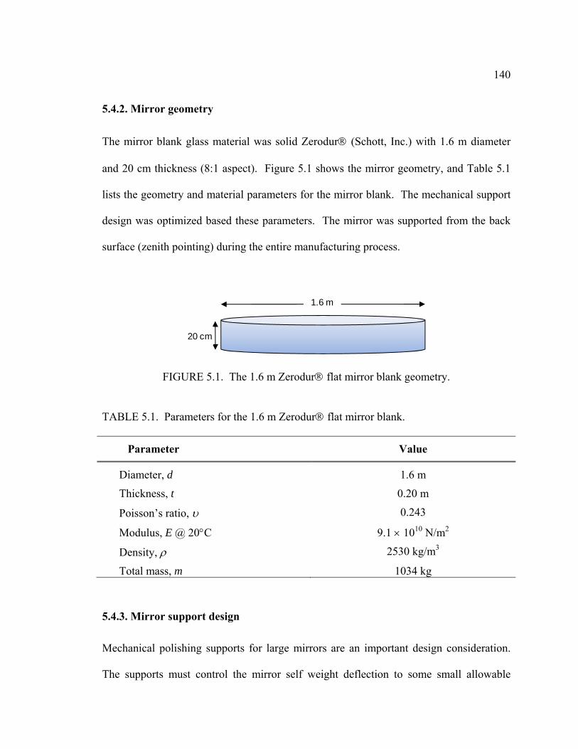
140

5.4.2. Mirror geometry

The mirror blank glass material was solid Zerodur® (Schott, Inc.) with 1.6 m diameter

and 20 cm thickness (8:1 aspect). Figure 5.1 shows the mirror geometry, and Table 5.1

lists the geometry and material parameters for the mirror blank. The mechanical support

design was optimized based these parameters. The mirror was supported from the back

surface (zenith pointing) during the entire manufacturing process.

FIGURE 5.1. The 1.6 m Zerodur® flat mirror blank geometry.

TABLE 5.1. Parameters for the 1.6 m Zerodur® flat mirror blank.

Parameter Value

Diameter, d 1.6 m

Thickness, t 0.20 m

Poisson’s ratio, υ 0.243

Modulus, E @ 20°C 9.1 × 1010 N/m2

Density, ρ 2530 kg/m3

Total mass, m 1034 kg

5.4.3. Mirror support design

Mechanical polishing supports for large mirrors are an important design consideration.

The supports must control the mirror self weight deflection to some small allowable

1.6 m

20 cm

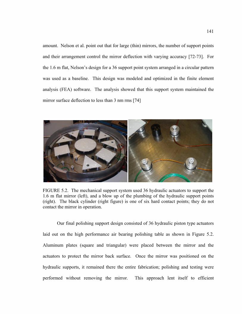
141

amount. Nelson et al. point out that for large (thin) mirrors, the number of support points

and their arrangement control the mirror deflection with varying accuracy [72-73]. For

the 1.6 m flat, Nelson’s design for a 36 support point system arranged in a circular pattern

was used as a baseline. This design was modeled and optimized in the finite element

analysis (FEA) software. The analysis showed that this support system maintained the

mirror surface deflection to less than 3 nm rms [74]

FIGURE 5.2. The mechanical support system used 36 hydraulic actuators to support the 1.6 m flat mirror (left), and a blow up of the plumbing of the hydraulic support points (right). The black cylinder (right figure) is one of six hard contact points; they do not contact the mirror in operation.

Our final polishing support design consisted of 36 hydraulic piston type actuators

laid out on the high performance air bearing polishing table as shown in Figure 5.2.

Aluminum plates (square and triangular) were placed between the mirror and the

actuators to protect the mirror back surface. Once the mirror was positioned on the

hydraulic supports, it remained there the entire fabrication; polishing and testing were

performed without removing the mirror. This approach lent itself to efficient

142

manufacturing. In addition, this approach minimized transfers of the mirrors and, thus,

risk of damaging the mirror.

5.4.4. Overview of the manufacturing sequence

The manufacture of large mirrors requires four phases: surface generation, grinding,

polishing, and figuring [10-11, 71]. We performed the grinding, polishing, and figuring.

After surface generation, the remaining three phases of the manufacture were carried out

in the following sequence:

1. First, we used a 100 cm diameter tool faced with ceramic tiles on the Draper machine

to grind out the generating marks and subsurface damage caused by the diamond

cutting tool. The same 100 cm tool was used with molded soft pitch to polish the

surface to a smooth finish and minimize power and asymmetrical surface variations.

The mirror rested on foam pads during this step.

2. During grinding and initial polishing, we periodically checked the global surface

changes with electronic levels. Polishing with the 100 cm tool continued until the

surface was smooth (with no visible marks and subsurface damage) and the measured

power in the mirror was 100 nm rms or better.

3. Next, the mirror was moved to the air bearing table and onto the hydraulic polishing

supports. We switched to smaller tools (size ranging from 15 to 40 cm diameters) for

polishing and figuring. A Draper machine was retrofitted with a radial stroker

(described in Section 4.5.8), which drove the smaller tools. (Note: We initially used

a 60 cm tool for surface figuring. After we failed to converge (Figure 5.12), we

switched to smaller tools and the radial stroker)

143

4. We used the scanning pentaprism system and the 1 m Fizeau interferometer to

monitor the mirror surface and guide the polishing/figuring.

5. We used polishing simulation software (described in Section 4.5.9) to help with the

polishing decisions. The software provided optimized tool stroke and dwell to reduce

the surface zones.

5.4.5. Large tool polishing

The grinding and coarse polishing were performed with a stiff 100 cm diameter tool on a

Draper machine. The tool applied about 0.3 pounds per square inch (psi) of pressure on

the mirror. Grinding was performed with tiles set in pitch on the work surface side of the

tool. For polishing, molded soft pitch in 10 cm squares was applied to the bottom of the

tool with about 1 cm channels between the squares. Before each polishing run, the tool

(with pitch) was first pressed out overnight on a flat surface. This step ensured a ‘flat’

tool at the beginning of a polishing run. Barnesite [11], a popular polishing compound

that has been used successfully at our facility, was used as the polishing compound or

slurry. To start polishing, the slurry was liberally applied to the mirror surface, and the

large tool was placed on top. The motions of the tool were adjusted based on the

measured surface data from the electronic levels and historical behavior of the large tool

with pitch and Barnesite. The tool was allowed to charge for a short time, after which it

was timed for the actual polishing run. Charging the surface refers to the process of the

polishing compound particles embedding themselves in pitch where they can remain

active for a period of time and is essential for efficient polishing. The mirror surface was

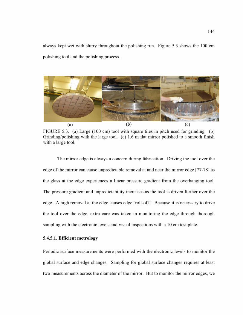
144

always kept wet with slurry throughout the polishing run. Figure 5.3 shows the 100 cm

polishing tool and the polishing process.

(a) (b) (c) FIGURE 5.3. (a) Large (100 cm) tool with square tiles in pitch used for grinding. (b) Grinding/polishing with the large tool. (c) 1.6 m flat mirror polished to a smooth finish with a large tool.

The mirror edge is always a concern during fabrication. Driving the tool over the

edge of the mirror can cause unpredictable removal at and near the mirror edge [77-78] as

the glass at the edge experiences a linear pressure gradient from the overhanging tool.

The pressure gradient and unpredictability increases as the tool is driven further over the

edge. A high removal at the edge causes edge ‘roll-off.’ Because it is necessary to drive

the tool over the edge, extra care was taken in monitoring the edge through thorough

sampling with the electronic levels and visual inspections with a 10 cm test plate.

5.4.5.1. Efficient metrology

Periodic surface measurements were performed with the electronic levels to monitor the

global surface and edge changes. Sampling for global surface changes requires at least

two measurements across the diameter of the mirror. But to monitor the mirror edges, we

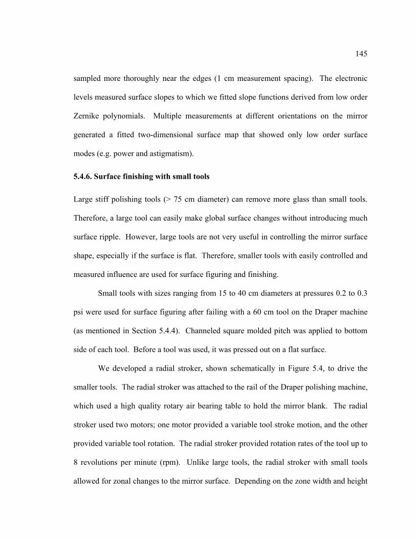
145

sampled more thoroughly near the edges (1 cm measurement spacing). The electronic

levels measured surface slopes to which we fitted slope functions derived from low order

Zernike polynomials. Multiple measurements at different orientations on the mirror

generated a fitted two-dimensional surface map that showed only low order surface

modes (e.g. power and astigmatism).

5.4.6. Surface finishing with small tools

Large stiff polishing tools (> 75 cm diameter) can remove more glass than small tools.

Therefore, a large tool can easily make global surface changes without introducing much

surface ripple. However, large tools are not very useful in controlling the mirror surface

shape, especially if the surface is flat. Therefore, smaller tools with easily controlled and

measured influence are used for surface figuring and finishing.

Small tools with sizes ranging from 15 to 40 cm diameters at pressures 0.2 to 0.3

psi were used for surface figuring after failing with a 60 cm tool on the Draper machine

(as mentioned in Section 5.4.4). Channeled square molded pitch was applied to bottom

side of each tool. Before a tool was used, it was pressed out on a flat surface.

We developed a radial stroker, shown schematically in Figure 5.4, to drive the

smaller tools. The radial stroker was attached to the rail of the Draper polishing machine,

which used a high quality rotary air bearing table to hold the mirror blank. The radial

stroker used two motors; one motor provided a variable tool stroke motion, and the other

provided variable tool rotation. The radial stroker provided rotation rates of the tool up to

8 revolutions per minute (rpm). Unlike large tools, the radial stroker with small tools

allowed for zonal changes to the mirror surface. Depending on the zone width and height

146

determined from the surface measurements, a proper tool size was chosen to reduce the

zone height by 40 to 50% in a single run. This conservative approach avoided removing

too much glass and creating a low zone. A low zone correction requires the entire

surface to be brought down to that level. The small tool was positioned over the high

zones by moving the Draper machine rail, which normally would provide stroke for large

polishing tools. Polishing simulation software, used to optimize the polishing tool stroke

and dwell, enabled computer control to correct the surface figure. We describe our

computer control polishing method next.

FIGURE 5.4. Schematic of the radial stroker and polishing/figuring with small tools. This radial stroker was attached to the Draper machine rail. Two motors provide variable tool stroke and rotation.

5.4.6.1. Computer controlled polishing

We developed computer controlled polishing for surface figuring through the use of

polishing simulation software. The computer control came from the choice of polishing

strokes based on computer simulation and optimization. The polishing simulation

software is based on the finite element modeling of the lap and glass mechanics and

Motor 1 provided stroke

Motor 2 provided rotation

Large f lat mirror

Radial stroker

on rotary air bearing polishing table

Small tool

147

assumed Preston’s relation, that glass removal rate is proportional to pressure and

velocity between the tool and the mirror. The software differed from most by allowing

the use of a rotating tool with a removal function that varies significantly with position of

the tool on the mirror [79]. The computation of the removal function at any point on the

mirror is made by numerically integrating Preston’s relation over the tool stroke position

and mirror rotation angle.

The software simulated polishing given the proper polishing parameters (i.e. tool

size, pressure and geometry, tool and mirror rotation speeds, etc.). Parameters such as

the tool dwell, stroke and position were then optimized for a particular surface zone.

Each surface zone required its own data file. Multiple zonal data files can be combined

to simulate their combined effect on the mirror. The design of the full polishing run was

then given to the optician to execute on the mirror.

In order to predict the surface removal, we first calibrated the Preston’s constant.

Preston’s equation is related to the rate of the material removal caused by the tool

velocity and pressure for each point on the mirror relative to the glass:

( ) vpKvpR ××=, . (5.1)

where R is the local removal rate

K is Preston’s proportionality constant (units µm/hr/psi/m/s)

p is the local tool pressure

v is the instantaneous linear velocity of the tool relative to the mirror surface.

Preston’s constant accounted for other parameters such as the behavior of the

polishing compound. To use the software successfully, the Preston’s constant first

148

required calibration by measuring the effects of the polishing strokes and tool dwell. The

result of our calibration of Preston’s constant is shown in Figure 5.5. A simple polishing

run was designed and simulated with the software. The simulation was then executed on

the mirror. The mirror surface was measured before and after this polishing run.

Preston’s constant was adjusted in software until simulated surface removal matched the

actual removal amplitude. The resulting constant was then recorded and stored for future

simulations. A typical value for our process was 15 µm/hr/psi/m/s.

FIGURE 5.5. The result of Preston’s constant calibration. In software Preston’s proportionality constant was adjusted until the simulated surface removal matched the actual removal amplitude.

For a mirror with only zonal errors, the radial surface profile can be written as

( ) ( )rfz ≤≤= ρρ 0, . (5.2)

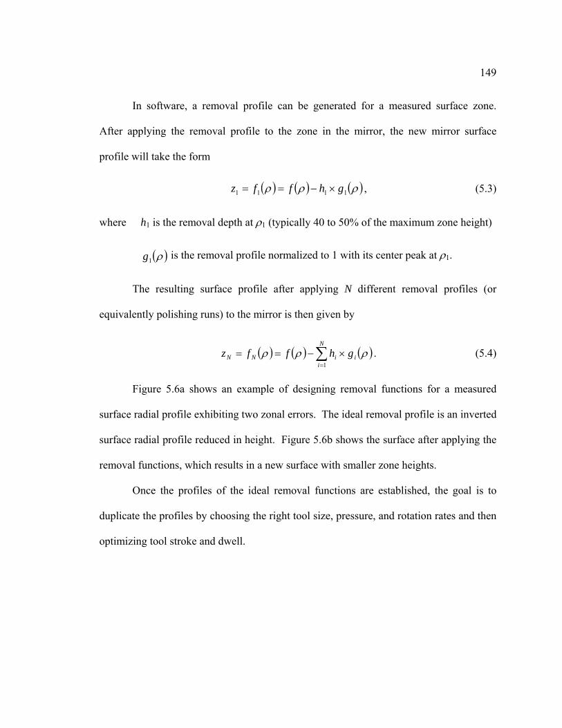
149

In software, a removal profile can be generated for a measured surface zone.

After applying the removal profile to the zone in the mirror, the new mirror surface

profile will take the form

( ) ( ) ( )ρρρ 1111 ghffz ×−== , (5.3)

where h1 is the removal depth at ρ1 (typically 40 to 50% of the maximum zone height)

( )ρ1g is the removal profile normalized to 1 with its center peak at ρ1.

The resulting surface profile after applying N different removal profiles (or

equivalently polishing runs) to the mirror is then given by

( ) ( ) ( )∑=

×−==N

iiiNN ghffz

1ρρρ . (5.4)

Figure 5.6a shows an example of designing removal functions for a measured

surface radial profile exhibiting two zonal errors. The ideal removal profile is an inverted

surface radial profile reduced in height. Figure 5.6b shows the surface after applying the

removal functions, which results in a new surface with smaller zone heights.

Once the profiles of the ideal removal functions are established, the goal is to

duplicate the profiles by choosing the right tool size, pressure, and rotation rates and then

optimizing tool stroke and dwell.

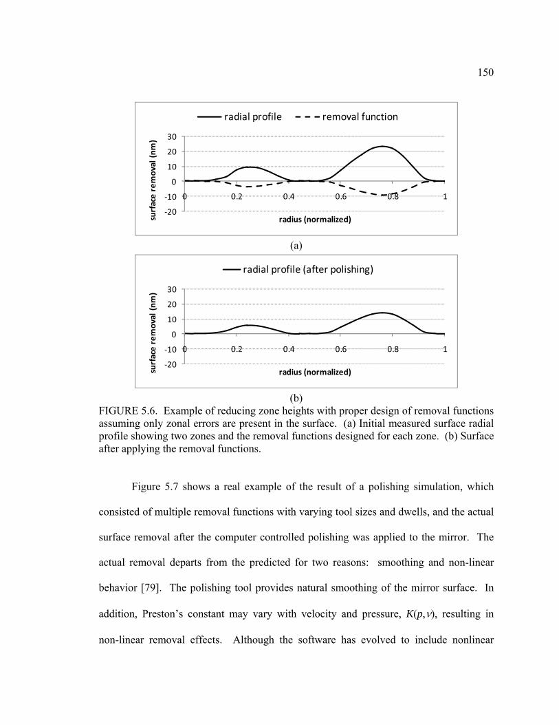
150

‐20

‐10

0

10

20

30

0 0.2 0.4 0.6 0.8 1

surface removal (nm

)

radius (normalized)

radial profile removal function

(a)

‐20

‐10

0

10

20

30

0 0.2 0.4 0.6 0.8 1

surface removal (nm

)

radius (normalized)

radial profile (after polishing)

(b)

FIGURE 5.6. Example of reducing zone heights with proper design of removal functions assuming only zonal errors are present in the surface. (a) Initial measured surface radial profile showing two zones and the removal functions designed for each zone. (b) Surface after applying the removal functions.

Figure 5.7 shows a real example of the result of a polishing simulation, which

consisted of multiple removal functions with varying tool sizes and dwells, and the actual

surface removal after the computer controlled polishing was applied to the mirror. The

actual removal departs from the predicted for two reasons: smoothing and non-linear

behavior [79]. The polishing tool provides natural smoothing of the mirror surface. In

addition, Preston’s constant may vary with velocity and pressure, K(p,ν), resulting in

non-linear removal effects. Although the software has evolved to include nonlinear

151

effects, this option was not used, because the magnitude of the nonlinear effects was not

known.

FIGURE 5.7. Comparison of a simulated and actual surface removal on the 1.6 m flat while it was in production.

Computer controlled polishing procedure

The method of computer controlled polishing was operated in a closed loop. A summary

of the steps for completing a computer controlled run is given next.

1. First, the mirror surface was measured with the scanning pentaprism system and the 1

m Fizeau interferometer, and the average radial profile of the mirror was then

calculated.

2. The average radial profile was imported into the polishing simulation software along

with the expected polishing parameters.

152

3. Inside the software the surface removal function for each zone was generated and

optimized. The target reduction for each zone was typically 40 to 50% of the

maximum zone height.

4. The surface removal on the measured average radial profile was then simulated, and

the result was evaluated.

5. Finally, the optimized polishing design was applied to the mirror. After the polishing

run was complete, the process was repeated from step 1.

Figure 5.8 shows the same closed loop sequence in a flowchart. Typically, polishing

runs required three to five hours to complete. This included time to change out polishing

tools and move the tool to other zones on the mirror. Multiple iterations of the above

sequence were carried out. In the next section, we present measurements obtained after

the final run. The method of closed loop computer controlled polishing convergence of

the surface figure was relatively rapid (an average of about 50 nm rms per week for

power as shown in Figure 5.12).

153

FIGURE 5.8. Flowchart diagram of the closed loop computer controlled polishing method.

5.4.6.2. Scanning pentaprism measurements for power

The result of the scanning pentaprism test on the finished mirror is shown in Figure 5.9.

The measurement was made along a single diagonal line on the mirror. Forward and

Measure and the surface with the scanning pentaprism

and 1 m Fizeau

Design removal functions for zones of interest

Optimize the simulation (tool stroke & dwell)

Apply the simulation to the mirror

Calculate and import the average radial prof ile into the polishing simulation sof tware

Power < 20 nm rmsIrregularity < 20 nm rms

Done

No

Yes

154

backward scans were performed and the data were averaged. Only low order

symmetrical Zernike polynomials were fitted to the data. The linear component of the fit

gives power. This measurement resulted in 11 nm rms power with measurement

uncertainty of 9 nm rms.

The large slopes due to surface irregularity were not represented well with low

order polynomials. Irregularity was more accurately measured interferometrically with

the 1 m Fizeau interferometer.

FIGURE 5.9. Measured slope data on the finished mirror with the scanning pentaprism along a single line and low order polynomial fit to the slope data. The linear component of the polynomial fit gives power in the surface (11 nm rms).

155

FIGURE 5.10. Result of the 1 m Fizeau measurement on the finished mirror. 24 subaperture measurements were acquired and combined with the maximum likelihood estimation (6 nm rms surface irregularity after removing power and astigmatism).

5.4.6.3. Fizeau measurements for surface irregularity

The surface map, shown in Figure 5.10, is the result of the 1 m Fizeau interferometer test

on the finished mirror. A total of 24 overlapping subaperture measurements were

acquired through multiple rotations of the reference and test surfaces. The subaperture

measurements were combined using the maximum likelihood estimation to get a full

surface map. Up to 188 Zernike terms were used to reconstruct the surface. Removing

power and astigmatism leaves surface irregularity of 6 nm rms with measurement

uncertainty of 3 nm rms. The results from stitching are not provided here but can be

found elsewhere [17, 90].

156

5.4.7. Demonstration of the flat mirror with 11 nm rms power and 6 nm rms surface irregularity

Figure 5.11 demonstrates the final surface map, which is the combination of the results

from the scanning pentaprism and Fizeau tests on the finished mirror: 11 nm rms power

and 6 nm rms surface irregularity. The final surface was characterized to 12.5 nm rms

and 57 nm peak to valley.

FIGURE 5.11. The final surface map showing combined power with surface irregularity from the scanning pentaprism and 1 m Fizeau tests on the finished mirror.

By continuing with the computer controlled polishing procedure described in

section 5.4.6.1 and based on the sensitivities of the test systems [47, 50], we estimated 6

nm (λ/100) rms power and 3 nm (λ/200) rms surface irregularity to be achievable for 2 m

157

class mirrors. Due to time constraints this state of the art surface figure of 6 nm rms

power and 3 nm rms irregularity was not achieved for the 1.6 m flat.

Figure 5.12 shows the rapid convergence of surface power on the 1.6 m flat

mirror after implementing our computer controlled polishing. Measurements on the left

side of the vertical dashed line were taken during classical large tool polishing before our

computer controlled polishing. The classical polishing method used a 60 cm polishing

tool to make corrections to the mirror surface. This method managed to bring the surface

to about 60 nm rms power before reversing direction on the error. After several more

polishing runs with the 60 cm tool and a dramatic increase in the surface power, we

switched to the closed loop computer controlled method.

‐0.05

0

0.05

0.1

0.15

0.2

0.25

0.3

1/1 1/11 1/21 1/31 2/10 2/20 3/2 3/12 3/22

Surface error (μm rms)

Date (2006)

Power trend in the flat

closed‐loop computer controlled

polishing

classicalpolishing

FIGURE 5.12. Power trend in the 1.6 meter flat (over about three months) as measured with the scanning pentaprism system. The power trend shows rapid convergence after implementing the polishing software aided computer controlled polishing.

158

5.5. Manufacture and Test Plan for a 4 m Flat Mirror

A key advantage of our manufacturing methodology described is that it is scalable to

larger mirrors. In this section we discuss the feasibility of extending our methodology to

4 m class mirrors.

5.5.1. Mirror geometry

Zerodur® (Schott Glass, Inc.), ULE® (Corning, Inc.), and fused quartz are common low

expansion glass materials for large mirror blanks. Each glass type has properties that

make it ideal for specific applications. Zerodur®, for example, has excellent opto-

thermal properties and chemical resistance, so it is typically chosen for space programs

and other extreme applications. For the purpose of the analysis below, we assumed a

solid Zerodur® mirror blank with a thickness of 10 cm shown in Figure 5.13 (40:1 aspect

ratio).

FIGURE 5.13. Solid Zerodur® 4 m flat mirror geometry.

5.5.2. Mirror support

Using the same approach described by Nelson et al. as a baseline (see Section 4.1.2), a

support system with 120 points, arranged on five rings, was modeled and optimized for a

mirror geometry described above. The support system arrangement is shown in Figure

4 m

10 cm

159

5.14. From the FEA modeling this support arrangement will maintain the mirror surface

deflection to about 12 nm rms after optimization [75-76].

FIGURE 5.14. A five ring support design for a 4 m mirror. This design will maintain the mirror deflection to about 12 nm rms.

5.5.3. Overview of the manufacturing sequence

Many of the same processes that were established during the manufacture of the 1.6 m

flat mirror can be used in larger mirror fabrication. After the mirror surface generation,

the manufacturing process might proceed as follows:

Courtesy of Brian C.Steward Mirror Lab

160

1. Use a large stiff tool (≥ 100 cm) with tiles to grind and then with pitch to polish the

surface to a smooth finish, minimize power and asymmetrical surface variations and

carefully monitor the edges.

2. Use the electronic levels to make surface slope measurements, monitor global surface

changes, and guide the initial polishing.

3. Switch to smaller tools (40 to 80 cm diameter) for figuring after the surface obtains a

smooth finish and power is less than 100 nm rms.

4. Use the scanning pentaprism and 1 m Fizeau tests to monitor the surface and guide

the remaining fabrication.

5. Use polishing simulation software to aid with the decisions on polishing and figuring.

Figure 5.15 shows the manufacturing sequence flowchart.

FIGURE 5.15. Potential manufacturing sequence for large high performance flat mirrors.

Grinding & coarse

polishing w/ large tools

Ef f icient metrology

Figuring w/ smaller tools

(ccp)

Ef f icient & accurate optical

metrology

Final f inished surface

4 m Draper machine Electronic levels

Air bearing table & hydraulic supports

Scanning pentaprism

11 nm rmspower

Conventional methods

Test plate to monitor edges Radial stroker 1 m Fizeau

interferometer6 nm rms

irregularity

Polishing simulation software

> 100 nm rms power > 11 nm rms power

> 6 nm rms irregularity

161

5.5.4. Limitations and risks

Because large mirrors may take a few years to complete, safety is a major concern when

handling mirror blanks that weigh three to five tons (4 m diameter). Damage to the

mirror blank is a significant risk especially during handling and transfer operations. We

minimize handling, however, by keeping the mirror on one table where it is well

supported (Section 5.2). Polishing and testing are performed without moving the mirror.

Additionally, shop risks can be mitigated through proper training and practice.

In this section, we look at other possible limitations and risks of our developed

fabrication and testing methods.

Fabrication: polishing and figuring

Our facility is currently limited to handling 4 m mirrors. Additional modifications to our

polishing table are necessary to accommodate mirrors larger than 4 m.

In addition, our large tool is limited to 100 cm in diameter. A 230 cm diameter or

larger tool, after characterization, can be used on a 4 m mirror for initial polishing. In

some cases, polishing techniques proven for smaller mirrors do not work for large

mirrors. As the tool size increases, so does the pressure it exerts on the mirror surface.

This alone may change the expected polishing outcome.

To succeed within the boundary of our capability, careful planning and design is

essential with special attention to gaining experience with tools and their effect on

mirrors in fabrication.

162

Surface slope testing

For a given magnitude surface error (e.g. 20 nm rms astigmatism) the surface slope errors

are inversely proportional to the mirror size. Thus, slope errors for a large mirror must

become smaller to maintain the same performance as a smaller one. For power, the edge

slope error is inversely proportional to the diameter of the mirror by (derived in the

Appendix)

Ds8

=Δθ , (5.5)

where s is the peak to valley power or sag in the mirror surface

D is the diameter of the mirror.

If the electronic levels, for example, are expected to measure 60 rms power in a 2

m mirror, then the edge slopes are 1 µrad. For the same specification on power for a 4 m

mirror, the edge slopes become 0.5 µrad. The sensitivities of the test systems must be

improved as the mirrors get larger.

We determined the measurement uncertainty in the electronic levels and the

scanning pentaprism system [46, 50]. The results shown in Table 5.2 are of Monte Carlo

simulations using the uncertainties in the slope test systems to estimate the accuracy in

measuring the low order Zernike aberrations in a 4 m flat mirror assuming 0.6 µrad rms

noise for the electronic levels test and 0.4 µrad rms noise for the scanning pentaprism

test. This analysis assumes three diagonal line scans and 12 measurement points per scan

for the electronic levels and 42 measurement points per scan for the scanning pentaprism.

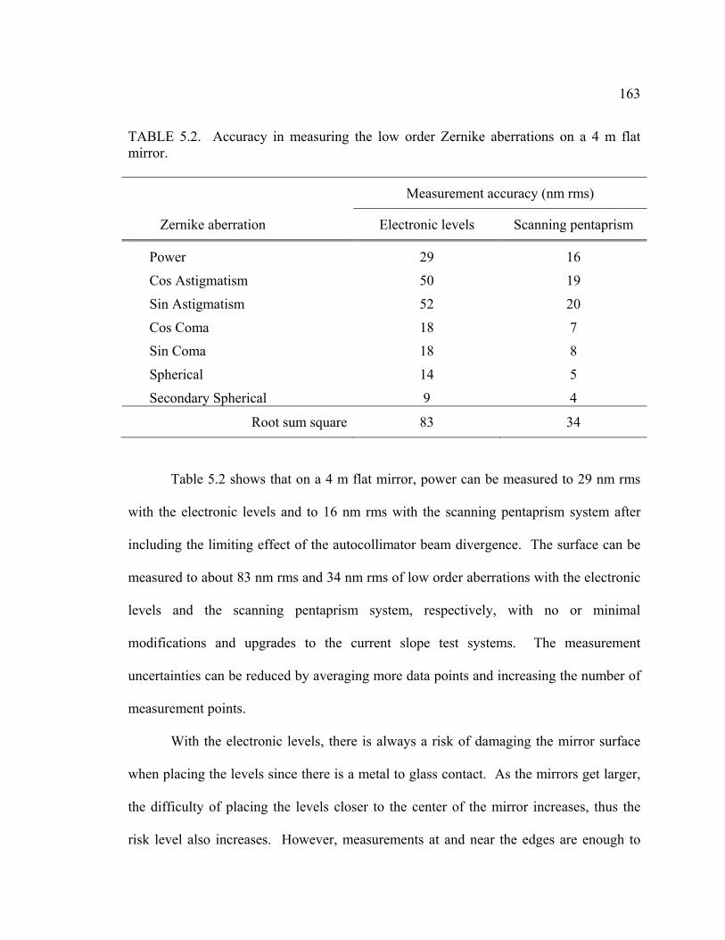
163

TABLE 5.2. Accuracy in measuring the low order Zernike aberrations on a 4 m flat mirror.

Measurement accuracy (nm rms)

Zernike aberration Electronic levels Scanning pentaprism

Power 29 16

Cos Astigmatism 50 19

Sin Astigmatism 52 20

Cos Coma 18 7

Sin Coma 18 8

Spherical 14 5

Secondary Spherical 9 4

Root sum square 83 34

Table 5.2 shows that on a 4 m flat mirror, power can be measured to 29 nm rms

with the electronic levels and to 16 nm rms with the scanning pentaprism system after

including the limiting effect of the autocollimator beam divergence. The surface can be

measured to about 83 nm rms and 34 nm rms of low order aberrations with the electronic

levels and the scanning pentaprism system, respectively, with no or minimal

modifications and upgrades to the current slope test systems. The measurement

uncertainties can be reduced by averaging more data points and increasing the number of

measurement points.

With the electronic levels, there is always a risk of damaging the mirror surface

when placing the levels since there is a metal to glass contact. As the mirrors get larger,

the difficulty of placing the levels closer to the center of the mirror increases, thus the

risk level also increases. However, measurements at and near the edges are enough to

164

measure global errors in the surface by Equation 5.2; measuring the slopes only at the

edges will reduce the risk of placing the electronic levels.

There is a potential limitation with the scanning pentaprism system: the current

system uses rails that are 2.5 m in length, so the current system may become limited in

size for flat mirrors 4 m in diameter or larger. Increasing the length of the rails

overcomes this limitation, but the increase does two things: increases the working

distance of the electronic autocollimator and picks up more noise over the longer beam

paths. Both these problems may limit the test system in accuracy. But more data

averaging can compensate for the additional noise and random errors.

Large Fizeau test

In the current Fizeau test the 1 m reference flat and test mirror are fixed in lateral

translation. This configuration limits how large a mirror we can test by subsampling (≤ 2

m). To measure larger mirrors, another degree of freedom in lateral translation is needed

for the reference flat.

Figure 5.16a shows the current subaperture sampling arrangement to measure 2 m

or smaller flat mirrors. The reference flat remains fixed and the test mirror is rotated

underneath to get full coverage. For a 1.6 m flat mirror eight subaperture measurements

are enough to get full coverage of the test mirror [47]. This type of sampling

arrangement is insufficient for flat mirrors larger than 2 m. Figure 5.16b shows an

example of subsampling a 4 m mirror after introducing lateral translation of the 1 m

reference flat. In this example, the reference flat is translated to three positions and the

test mirror is rotated underneath to acquire 25 subaperture measurements and provide full

165

coverage of the mirror. All 25 measurements must be combined to get a full synthetic

surface map.

Current Fizeau test system - 1 m subsampling of a 1.6 m flat mirror

Additional degree of freedom of the reference - example subsampling of a 4 m flat mirror

(a) (b)

FIGURE 5.16. (a) 1 m subaperture (dashed circular outlines) sampling on the 1.6 m flat mirror, and (b) on a 4 m flat mirror. Multiple subaperture sampling provides full coverage of the large mirror. Combining the subaperture measurements produces a full synthetic map.

Errors in stitching the subaperture measurements increase as more subapertures

are combined. The increase in subaperture measurements limits the accuracy of the test

system. However, the quality of the test in terms of slope, power spectral density or

structure function is not degraded.

5.6. Conclusion

The manufacture of large flat mirrors is challenging. We found classical polishing alone

does not enable the manufacture of large high performance flat mirror much larger than 1

166

m diameter. We reported on the methodology and enabling technologies for fabricating

and testing high performance large flat mirrors. We developed the enabling fabrication

and testing technologies during the manufacture of a 1.6 m flat mirror that measured 11

nm (λ/60) rms in power and 6 nm (λ/100) rms in surface irregularity on the finished

mirror. The enabling technologies are scalable for manufacture of flat mirrors as large as

8 m in diameter with proper tool design and selection. Our discussion of limitations and

risks showed the accurate manufacture of a 4 m flat mirror is within our current

capability.

167

CONCLUSION

A description of the methodology for manufacturing large high performance flat mirrors

that are much larger then 1 m diameter and of solid (i.e. non light weighted) glass

material has been given. We found during the manufacture of a 1.6 meter flat mirror that

classical fabrication methods alone do not enable fabrication of quality large flats and

current metrology for large flats are limited in efficiency and accuracy. To address these

limitations, we developed computer controlled polishing that used polishing simulation

software combined with accurate and efficient metrology. Two slope tests, the electronic

levels and scanning pentaprism, were developed and analyzed in detail. A vibration

insensitive interferometer, based on the classical Fizeau, with an external 1 meter

reference flat was developed, characterized, and calibrated. The Fizeau interferometer

used subaperture sampling and stitching and maximum likelihood estimation to obtain

synthetic surface maps over the full aperture of the flat mirror.

The electronic levels were used during early fabrication (grinding and coarse

polishing with large tools) to provide efficient determination of global changes in the

mirror surface. The scanning pentaprism and the 1 m Fizeau are highly accurate tests and

were used during the remaining fabrication and to qualify the surface figure of the

finished mirror. The surface of the finished 1.6 m flat was measured to 11 nm rms (±9

nm rms) power and 6 nm rms (±3 nm rms) surface irregularity. At present this is the best

large flat in the world.

168

The analysis of the risks and limitations of the fabrication methods and metrology

showed that manufacturing 4 m flat mirrors is within our current capabilities. Mirrors

larger than 4 meters will require modifying mechanics including the polishing machines,

metrology and data analysis techniques. Changes to the fabrication include designing

larger stiff tools and carefully characterizing them. Changes to the metrology include

increasing the data averaging and introducing an additional degree of freedom in lateral

translation for the Fizeau reference flat.

The manufacture of large flat mirror is challenging. We addressed the limitations

and laid the foundation for flat fabrication by developing enabling fabrication and testing

technologies. Our method of computer controlled polishing was operated in closed loop.

The key advantage to our methodology is it is scalable to 8 meter flat mirrors. With

proper design of the mechanics and hardware, including polishing tools, and upgrades to

the data analysis software, high performance 8 meter flat mirrors are possible in the

future.

The amount of work it took to finish this project was a lot more than one person

can handle. It took a tremendous team effort to develop and implement the method of

large flat manufacturing described in this dissertation and produce a very high

performance 2 m class flat mirror. In addition to my role as the lead systems engineer on

this project, I developed the electronic levels test, performed extensive analysis on the

electronic levels and scanning pentaprism test systems, resulting in improved accuracies,

designed polishing runs using predictive software and measured data, and, finally,

integrated the metrology and fabrication methods into a closed loop manufacturing

169

operation that eventually produced the world’s best 2 m class flat. Individuals that

directly contributed technical solutions to this project were acknowledged in the

beginning.

170

APPENDIX A

EDGE SLOPES FROM SURFACE CURVATURE

The sag in a mirror surface is defined as

R

rs2

2

= (A.1)

where r is the semi-diameter of the mirror and R is the radius of curvature. The slope in

the radial direction is then

( )Rr

drdsr ==θ (A.2)

or

( )rs

rr

Rrr 2

22

=⎟⎠⎞

⎜⎝⎛⋅=θ (A.3)

The difference between the edge slopes is now

DsDD 8

22=⎟

⎠⎞

⎜⎝⎛−−⎟

⎠⎞

⎜⎝⎛=Δ θθθ , (A.4)

where D is the diameter of the mirror. Rearranging Equation A.4 shows slope

measurements on opposing edges of the mirror are enough to measure the global

curvature in the surface.

8θΔ⋅

=Ds . (A.5)

171

APPENDIX B

SCANNING PENTAPRISM TEST MONTE CARLO ANALYSIS OF NOISE COUPLING INTO MID ORDER ZERNIKE ABERRATIONS FOR NUMBER OF LINE SCANS, NUMBER OF MEASUREMENT

POINTS AND LINE SCAN OFFSETS

This analysis is a continuation from Section 3.4.10. The Monte Carlo analysis studied

measurement noise normalized to 1 μrad rms coupling into mid order Zernike aberrations

(defined in Table 3.7). The parameters that were varied are the number of line scans

(three to six), number of measurement points per scan, and the distance of the line scans

from the center of the mirror (offset). The line scans were spaced in angle such that scans

were symmetrical around the mirror.

The proceeding plots are for the case when the line scans had no offsets (i.e. the

line scans go through the center of the mirror). The amounts of measurement error due to

measurement noise are plotted against the number of measurement points (for each

number of line scans). A function of the form 2/1−AN was then fitted to the data points,

where the A coefficient is the sensitivity to noise and N is the number of measurement

points. The value of the A coefficient was chose that resulted in the best fit to the data

points. The function shows that the measurement error decreases as N1 . The sampling

spacing was varied to obtain a distribution of data points for the measurement error.

Summary of the proceeding plots (Figures B.1 through B.10):

172


order Zernike aberrations for a 2 m flat mirror.

2. The line scans have no offset.

3. Sampling of trefoil (3θ) requires a minimum of four line scans

4. Ssampling of pentafoil (4θ) requires a minimum of five line scans.

5. The plots generally follow 2/1−AN .

TABLE B.1. Values of the A coefficient for the mid order Zernike aberrations for the case of the line scans with no offset.

Trefoil Secondary

astigmatism Secondary

coma Pentafoil Higher order

spherical

Line scans Z10 Z11 Z12 Z13 Z14 Z15 Z17 Z18 Z16 Z25

3 -- -- 115 115 40 40 -- -- 35 25 4 190 190 58 60 35 36 -- -- 33 22

5 165 170 53 53 33 33 97 99 29 21

6 155 157 50 49 30 29 92 94 26 20

173

1

10

100

1 10 100 1000

Measurement error (nm

rms)


Cos trefoil (Z10) sensitivity (4 line scan)

1

10

100

1 10 100 1000


rms)



1

10

100

1 10 100 1000


rms)



FIGURE B.1. Measurement noise normalized to 1 µrad coupling into cos trefoil (Z10) for the number of line scans and number of measurement points over a 2 m flat.

174

1

10

100

1 10 100 1000


rms)


Sin trefoil (Z11) sensitivity (4 line scan)

1

10

100

1 10 100 1000


rms)



1

10

100

1 10 100 1000


rms)



FIGURE B.2. Measurement noise normalized to 1 µrad coupling into sin trefoil (Z11) for the number of line scans and number of measurement points over a 2 m flat.

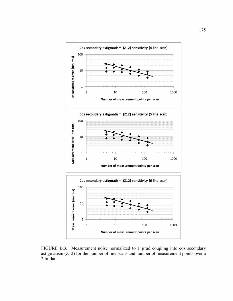
175

1

10

100

1 10 100 1000


rms)


Cos secondary astigmatism (Z12) sensitivity (4 line scan)

1

10

100

1 10 100 1000


rms)



1

10

100

1 10 100 1000


rms)



FIGURE B.3. Measurement noise normalized to 1 µrad coupling into cos secondary astigmatism (Z12) for the number of line scans and number of measurement points over a 2 m flat.

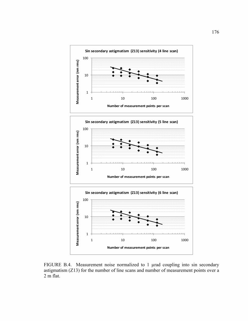
176

1

10

100

1 10 100 1000


rms)


Sin secondary astigmatism (Z13) sensitivity (4 line scan)

1

10

100

1 10 100 1000


rms)



1

10

100

1 10 100 1000


rms)



FIGURE B.4. Measurement noise normalized to 1 µrad coupling into sin secondary astigmatism (Z13) for the number of line scans and number of measurement points over a 2 m flat.

177

1

10

100

1 10 100 1000


rms)


Cos secondary coma (Z14) sensitivity (4 line scan)

1

10

100

1 10 100 1000


rms)



1

10

100

1 10 100 1000


rms)



FIGURE B.5. Measurement noise normalized to 1 µrad coupling into cos secondary coma (Z14) for the number of line scans and number of measurement points over a 2 m flat.

178

1

10

100

1 10 100 1000


rms)


Sin secondary coma (Z15) sensitivity (4 line scan)

1

10

100

1 10 100 1000


rms)



1

10

100

1 10 100 1000


rms)



FIGURE B.6. Measurement noise normalized to 1 µrad coupling into sin secondary coma (Z15) for the number of line scans and number of measurement points over a 2 m flat.

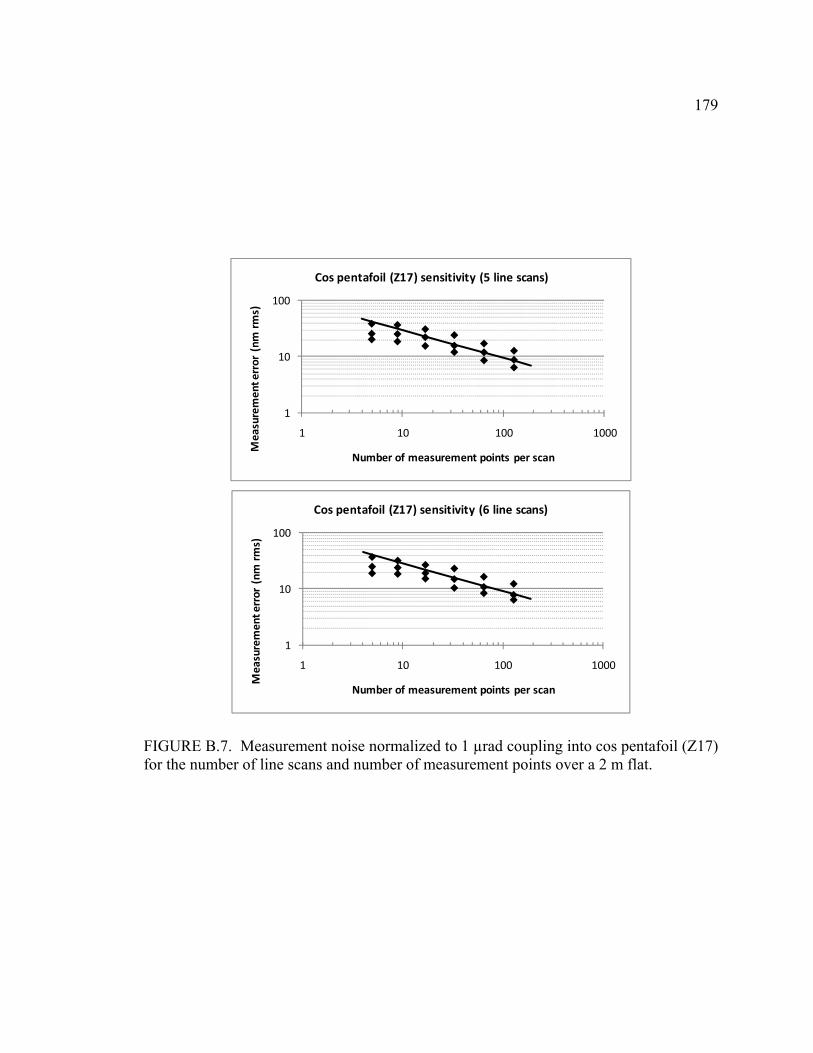
179

1

10

100

1 10 100 1000


rms)


Cos pentafoil (Z17) sensitivity (5 line scans)

1

10

100

1 10 100 1000


rms)


Cos pentafoil (Z17) sensitivity (6 line scans)

FIGURE B.7. Measurement noise normalized to 1 µrad coupling into cos pentafoil (Z17) for the number of line scans and number of measurement points over a 2 m flat.

180

1

10

100

1 10 100 1000


rms)


Sin pentafoil (Z18) sensitivity (5 line scans)

1

10

100

1 10 100 1000


rms)


Sin pentafoil (Z18) sensitivity (6 line scans)

FIGURE B.8. Measurement noise normalized to 1 µrad coupling into sin pentafoil (Z18) for the number of line scans and number of measurement points over a 2 m flat

181

1

10

100

1 10 100 1000


rms)


Secondary spherical (Z16) sensitivity (4 line scan)

1

10

100

1 10 100 1000


rms)



1

10

100

1 10 100 1000


rms)



FIGURE B.9. Measurement noise normalized to 1 µrad coupling into secondary spherical (Z16) for the number of line scans and number of measurement points over a 2 m flat.

182

1

10

100

1 10 100 1000


rms)


Tertiary spherical (Z25) sensitivity (4 line scan)

1

10

100

1 10 100 1000


rms)



1

10

100

1 10 100 1000


rms)



FIGURE B.10. Measurement noise normalized to 1 µrad coupling into tertiary spherical (Z25) for the number of line scans and number of measurement points over a 2 m flat.

183

The proceeding plots are for the case when the line scans offsets was 250 mm as shown

in Figure B.11. The amounts of measurement error due to measurement noise are plotted

against the number of measurement points (for each number of line scans). A function of

the form 2/1−AN was fitted to the data points, where A coefficient is the sensitivity to

noise and N is the number of measurement points. Only the fitted functions are plotted to

get all the number of line scans in a single plot.




2. The line scans have 250 mm offset from the mirror center.

3. Sampling of trefoil (3θ) requires a minimum of four line scans.

4. Sampling of pentafoil (4θ) requires a minimum of five line scans.

5. The plots generally follow 2/1−AN (Note: Except for small N due to under sampling).

TABLE B.2. Values of the A coefficient for the mid order Zernike aberrations for the case of the line scans with 250 mm offsets.

Trefoil Secondary


coma Pentafoil High order spherical


3 -- -- 50 49 36 36 -- -- 39 30 4 122 125 34 52 30 29 -- -- 37 25

5 108 110 38 39 27 27 92 90 29 22

6 100 102 35 35 26 25 82 82 27 21

184

(a) (b)

(c) (d)

FIGURE B.11. Scanning pentaprism test examples – line scans (three, four, five, and six) are offset from the center of a 2 m mirror by 250 mm. The line scans are spaced in angle such that the scans are symmetrical around the mirror.

185

1

10

100

1 10 100

Normalized

measurement error (nm rm

s)


Cos trefoil (Z10) sensitivity (250 mm scan offset)

4 line scans

5 line scans

6 line scans

1

10

100

1 10 100

Normalized


s)


Sin trefoil (Z11) sensitivity (250 mm scan offset)

4 line scans

5 line scans

6 line scans

FIGURE B.12. Measurement noise normalized to 1 μrad rms coupling into trefoil (Z10, Z11) for number of line scans, number of measurement points, and d = 250 mm.

186

1

10

100

1 10 100

Normalized


s)


Cos secondary astigmatism (Z12) sensitivity (250 mm scan offset)

3 line scans

4 line scans

5 line scans

6 line scans

1

10

100

1 10 100

Normalized


s)


Sin secondary astigmatism (Z13) sensitivity (250 mm scan offset)

3 line scans

4 line scans

5 line scans

6 line scans

FIGURE B.13. Measurement noise normalized to 1 μrad rms coupling into secondary astigmatism (Z12, Z13) for number of line scans, number of measurement points, and d = 250 mm.

187

1

10

100

1 10 100

Normalized

easurem

ent error (nm rm

s)


Cos secondary coma (Z14) sensitivity (250 mm scan offset)

3 line scans

4 line scans

5 line scans

6 line scans

1

10

100

1 10 100

Normalized


s)


Sin secondary coma (Z15) sensitivity ( 250 mm scan offset)

3 line scans

4 line scans

5 line scans

6 line scans

FIGURE B.14. Measurement noise normalized to 1 μrad rms coupling into secondary coma (Z14, Z15) for number of line scans, number of measurement points, and d = 250 mm.

188

1

10

100

1 10 100

Normalized


s)


Cos pentafoil (Z17) sensitivity (250 mm scan offset)

5 line scans

6 line scans

1

10

100

1 10 100

Normalized


s)


Sin pentafoil (Z18) sensitivity (250 mm scan offset)

5 line scans

6 line scans

FIGURE B.15. Measurement noise normalized to 1 μrad rms coupling into pentafoil or 4θ (Z17, Z18) for number of line scans, number of measurement points, and d = 250 mm.

189

1

10

100

1 10 100

Normalized


s)


Secondary spherical (Z16) sensitivity (250 mm scan offset)

3 line scans

4 line scans

5 line scans

6 line scans

1

10

100

1 10 100

Normalized


s)


Tertiary spherical (Z25) sensitivity (250 mm scan offset)

3 line scans

4 line scans

5 line scans

6 line scans

FIGURE B.16. Measurement noise normalized to 1 μrad rms coupling into secondary and tertiary spherical (Z16, Z25) for number of line scans, number of measurement points, and d = 250 mm.

190

The proceeding plots are for the case when the line scans offsets was 500 mm as shown

in Figure B.17. The amounts of measurement error due to measurement noise are plotted

against the number of measurement points (for each number of line scans). A function of

the form 2/1−AN was fitted to the data points, where A coefficient is the sensitivity to

noise and N is the number of measurement points. Only the fitted functions are plotted to

get all the number of line scans in a single plot.




2. The line scans have 500 mm offset from the mirror center.

3. Sampling of trefoil (3θ) requires a minimum of four line scans.

4. Sampling of pentafoil (4θ) requires a minimum of five line scans.

5. The plots generally follow 2/1−AN (Note: Except for small N due to under sampling).

TABLE B.3. Values of the A coefficient for the mid order Zernike aberrations for the case of the line scans with 500 mm offsets.

Trefoil Secondary


coma Pentafoil Higher order

spherical


3 -- -- 103 97 65 65 -- -- 49 38 4 90 88 59 35 35 32 -- -- 46 32

5 91 91 44 45 37 36 95 93 37 28

6 128 55 50 48 28 27 100 97 32 25

191

(a) (b)

(c) (d)

FIGURE B.17. Scanning pentaprism test examples – line scans (three, four, five, and six) are offset from the center of a 2 m mirror by 250 mm. The line scans are spaced in angle such that scans are symmetrical around the mirror.

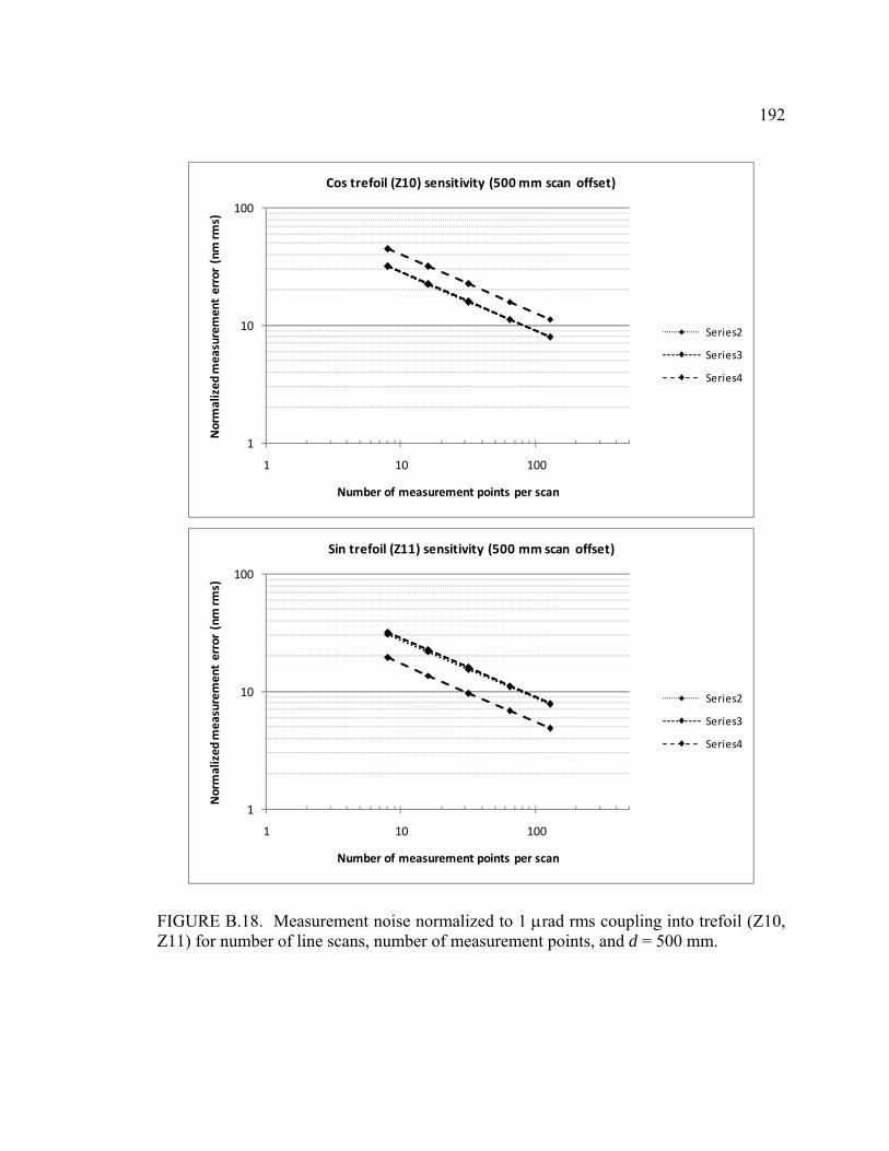
192

1

10

100

1 10 100

Normalized


s)


Cos trefoil (Z10) sensitivity (500 mm scan offset)

Series2

Series3

Series4

1

10

100

1 10 100

Normalized


s)


Sin trefoil (Z11) sensitivity (500 mm scan offset)

Series2

Series3

Series4

FIGURE B.18. Measurement noise normalized to 1 μrad rms coupling into trefoil (Z10, Z11) for number of line scans, number of measurement points, and d = 500 mm.

193

1

10

100

1 10 100

Normalized


s)


Cos secondary astigmatism (Z12) sensitivity (500 mm scan offset)

Series1

Series2

Series3

Series4

1

10

100

1 10 100

Normalized


s)


Sin secondary astigmatism (Z13) sensitivity (500 mm scan offset)

Series1

Series2

Series3

Series4

FIGURE B.19. Measurement noise normalized to 1 μrad rms coupling into secondary astigmatism (Z12, Z13) for number of line scans, number of measurement points, and d = 500 mm.

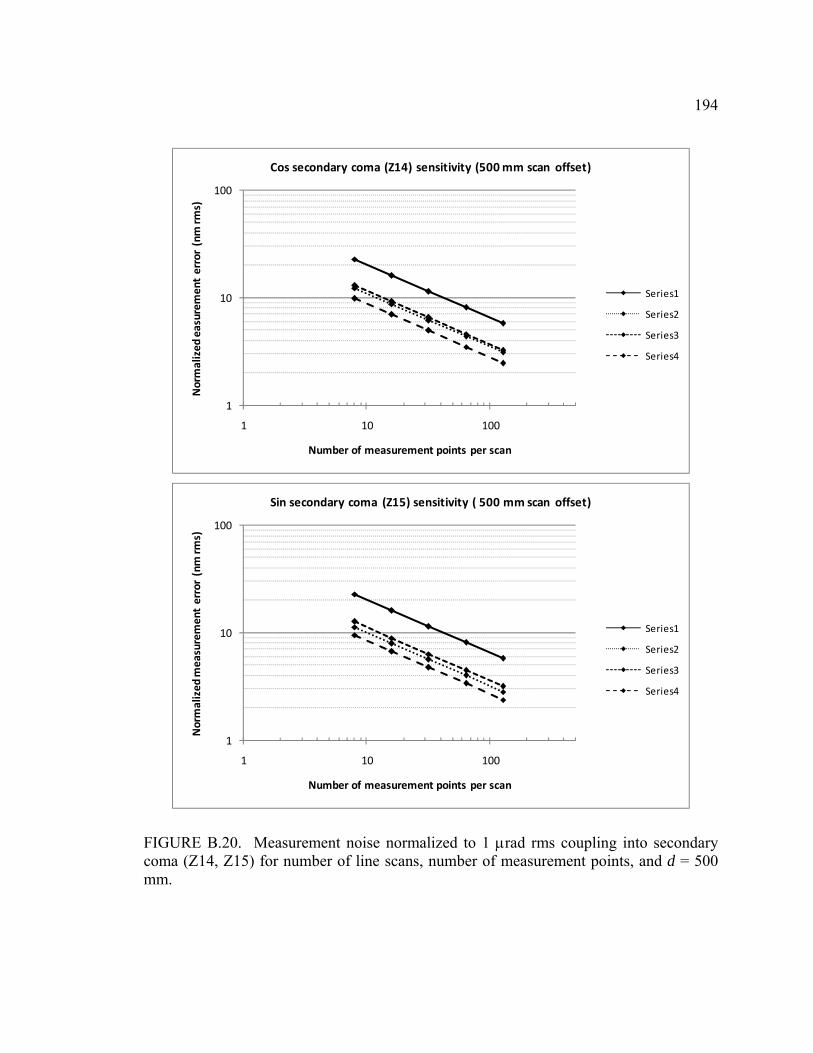
194

1

10

100

1 10 100

Normalized

easurem

ent error (nm rm

s)


Cos secondary coma (Z14) sensitivity (500 mm scan offset)

Series1

Series2

Series3

Series4

1

10

100

1 10 100

Normalized


s)


Sin secondary coma (Z15) sensitivity ( 500 mm scan offset)

Series1

Series2

Series3

Series4

FIGURE B.20. Measurement noise normalized to 1 μrad rms coupling into secondary coma (Z14, Z15) for number of line scans, number of measurement points, and d = 500 mm.

195

1

10

100

1 10 100

Normalized


s)


Cos pentafoil (Z17) sensitivity (500 mm scan offset)

Series1

Series2

1

10

100

1 10 100

Normalized


s)


Sin pentafoil (Z18) sensitivity (500 mm scan offset)

Series1

Series2

FIGURE B.21. Measurement noise normalized to 1 μrad rms coupling into pentafoil or 4θ (Z17, Z18) for number of line scans, number of measurement points, and d = 500 mm.

196

1

10

100

1 10 100

Normalized


s)


Secondary spherical (Z16) sensitivity (500 mm scan offset)

Series1

Series7

Series2

Series3

1

10

100

1 10 100

Normalized


s)


Tertiary spherical (Z25) sensitivity (500 mm scan offset)

Series1

Series7

Series2

Series3

FIGURE B.22. Measurement noise normalized to 1 μrad rms coupling into secondary and tertiary spherical (Z16, Z25) for number of line scans, number of measurement points, and d = 500 mm.

197

The next set of plots shows the same data (measurement noise normalized to 1 µrad rms

coupling into mid order Zernike aberrations), but plotted against the line scans distance

from the center of the mirror or offset, d. The set of plots assumes 64 measurement

points per line scan. The number of measurement points is maintained for each line scan

with offset.




2. The set of plots assumes 64 measurement points per line scan.

3. The behaviors of the measurement errors are mixed; some aberrations get sampled

better with increasing line scan offsets, while others do not.

4. For some aberrations their trends are also mixed (e.g. secondary astigmatism).

5. Due to mixed behaviors, some aberrations get sampled better with a combination of

the number of line scans and line scan offsets. For example, pentafoil is sampled well

with six line scans and 250 mm line scan offset.

198

0

5

10

15

20

25

0 100 200 300 400 500

Normalized


s)

Scan offset from center (mm)

Cos trefoil (Z10) sensitivity (64 points per scan)

4 line scans

5 line scans

6 line scans

0

5

10

15

20

25

0 100 200 300 400 500

Normalized


s)


Sin trefoil (Z11) sensitivity (64 points per scan)

4 line scans

5 line scans

6 line scans

FIGURE B.23. Measurement noise normalized to 1 μrad rms coupling into trefoil (Z10, Z11) for number of line scans and 64 measurement points.

199

0

2

4

6

8

10

12

14

16

0 100 200 300 400 500

Normalized


s)


Cos secondary astigmatism (Z12) sensitivity (64 points per scan)

3 line scans

4 line scans

5 line scans

6 line scans

0

2

4

6

8

10

12

14

16

0 100 200 300 400 500

Normalized


s)


Sin secondary astigmatism (Z13) sensitivity (64 points per scan)

3 line scans

4 line scans

5 line scans

6 line scans

FIGURE B.24. Measurement noise normalized to 1 μrad rms coupling into secondary astigmatism (Z12, Z13) for number of line scans and 64 measurement points.

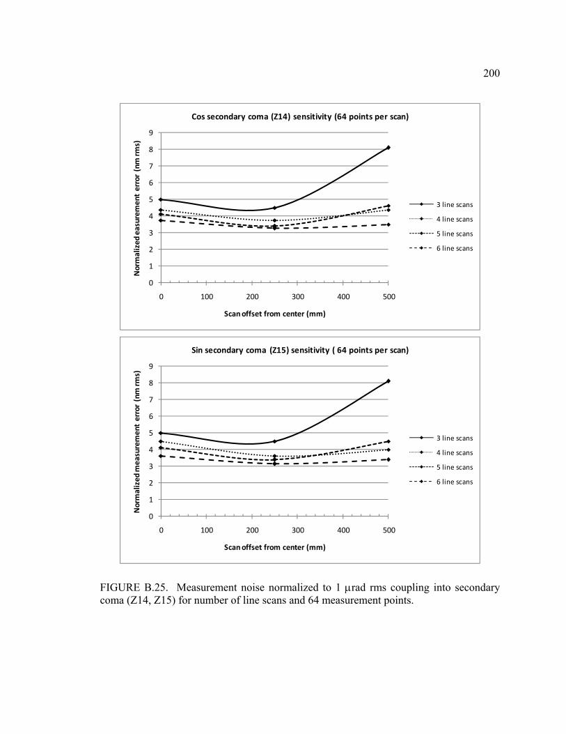
200

0

1

2

3

4

5

6

7

8

9

0 100 200 300 400 500

Normalized

easurem

ent error (nm rm

s)


Cos secondary coma (Z14) sensitivity (64 points per scan)

3 line scans

4 line scans

5 line scans

6 line scans

0

1

2

3

4

5

6

7

8

9

0 100 200 300 400 500

Normalized


s)


Sin secondary coma (Z15) sensitivity ( 64 points per scan)

3 line scans

4 line scans

5 line scans

6 line scans

FIGURE B.25. Measurement noise normalized to 1 μrad rms coupling into secondary coma (Z14, Z15) for number of line scans and 64 measurement points.

201

0

2

4

6

8

10

12

14

0 100 200 300 400 500

Normalized


s)


Cos pentafoil (Z17) sensitivity (64 points per scan)

5 line scans

6 line scans

0

2

4

6

8

10

12

14

0 100 200 300 400 500

Normalized


s)


Sin pentafoil (Z18) sensitivity (64 points per scan)

5 line scans

6 line scans

FIGURE B.26. Measurement noise normalized to 1 μrad rms coupling into pentafoil or 4θ (Z17, Z18) for number of line scans and 64 measurement points.

202

0

1

2

3

4

5

6

7

0 100 200 300 400 500

Normalized


s)


Secondary spherical (Z16) sensitivity (64 points per scan)

3 line scans

4 line scans

5 line scans

6 line scans

0

0.5

1

1.5

2

2.5

3

3.5

4

4.5

5

0 100 200 300 400 500

Normalized


s)


Tertiary spherical (Z25) sensitivity (64 points per scan)

3 line scans

4 line scans

5 line scans

6 line scans

FIGURE B.27. Measurement noise normalized to 1 μrad rms coupling into secondary and tertiary spherical (Z16, Z25) for number of line scans and 64 measurement point per scan.

203

The next set of plots shows the same data (measurement noise normalized to 1 µrad rms

coupling into mid order Zernike aberrations), but plotted against the number of line

scans. The set of plots assumes 64 measurement points per scan. The number of

measurement points is maintained for the line scans with offset.




2. The set of plots assumes 64 measurement points per line scan.

3. The behavior of the measurement errors differ between the aberrations due to the

ability of certain line scans with certain offsets to sample aberrations better. For

example, secondary astigmatism and coma are sampled well with six line scans and

500 mm line scan offset, while secondary and tertiary spherical are sampled well with

six line scans with no offset.

204

0

5

10

15

20

25

1 2 3 4 5 6 7

Normalized


s)

Number of line scans

Cos trefoil (Z10) sensitivity (64 points per scan)

d = 0mm

d = 250mm

d = 500mm

0

5

10

15

20

25

1 2 3 4 5 6 7

Normalized


s)


Sin trefoil (Z11) sensitivity (64 points per scan)

d = 0mm

d = 250mm

d = 500mm

FIGURE B.28. Measurement noise normalized to 1 µrad rms coupling into trefoil (Z10, Z11) for number of line scans and 64 measurement points per scan.

205

0

2

4

6

8

10

12

14

16

1 2 3 4 5 6 7

Normalized


s)


Cos secondary astigmatism (Z12) sensitivity (64 points per scan)

d = 0mm

d = 250mm

d = 500mm

0

2

4

6

8

10

12

14

16

1 2 3 4 5 6 7

Normalized


s)


Sin secondary astigmatism (Z13) sensitivity (64 points per scan)

d = 0mm

d = 250mm

d = 500mm

FIGURE B.29. Measurement noise normalized to 1 µrad rms coupling into secondary astigmatism (Z12, Z13) for number of line scans and 64 measurement points per scan.

206

0

1

2

3

4

5

6

7

8

9

1 2 3 4 5 6 7

Normalized

easurem

ent error (nm rm

s)


Cos secondary coma (Z14) sensitivity (64 points per scan)

d = 0mm

d = 250mm

d = 500mm

0

1

2

3

4

5

6

7

8

9

1 2 3 4 5 6 7

Normalized


s)


Sin secondary coma (Z15) sensitivity ( 64 points per scan)

d = 0mm

d = 250mm

d = 500mm

FIGURE B.30. Measurement noise normalized to 1 µrad rms coupling into secondary coma (Z14, Z15) for number of line scans and 64 measurement points per scan.

207

0

2

4

6

8

10

12

14

1 2 3 4 5 6 7

Normalized


s)


Cos pentafoil (Z17) sensitivity (64 points per scan)

d = 0mm

d = 250mm

d = 500mm

0

2

4

6

8

10

12

14

1 2 3 4 5 6 7

Normalized


s)


Sin pentafoil (Z18) sensitivity (64 points per scan)

d = 0mm

d = 250mm

d = 500mm

FIGURE B.31. Measurement noise normalized to 1 µrad rms coupling into pentafoil or 4θ (Z17, Z18) for number of line scans and 64 measurement points per scan.

208

0

1

2

3

4

5

6

7

1 2 3 4 5 6 7

Normalized


s)


Secondary spherical (Z16) sensitivity (64 points per scan)

d = 0mm

d = 250mm

d = 500mm

0

0.5

1

1.5

2

2.5

3

3.5

4

4.5

5

1 2 3 4 5 6 7

Normalized


s)


Tertiary spherical (Z25) sensitivity (64 points per scan)

d = 0mm

d = 250mm

d = 500mm

FIGURE B.32. Measurement noise normalized to 1 µrad rms coupling into secondary and tertiary spherical (Z16, Z25) for number of line scans and 64 measurement points per scan.

209

REFERENCES

[1] J. W. Mayo, III, “Problem areas in large optics fabrication – a project manager’s perspective,” Proc. SPIE 542, 1 (1985).

[2] G. Bilie, M. Weijun, “The experiment of Φ1m annular continuous polisher (ACP) for LAMOST ultrathin hexagonal flat,” Proc. SPIE 3785, 94 (1999).

[3] L. V. Bourimborde, A. Tonso, L. M. Zerbino, M. Garavaglaia, “Optical interference studies of a confined liquid free surface: meniscus effect compensation and time evolution of the surface, Opt. Eng. 35 (1), 70 (1996).

[4] D. A. Ketelsen, D. S. Anderson, “Optical testing with large liquid flats,” Proc. SPIE 966, 365 (1988).

[5] I. Powell, E. Goulet, “Absolute figure measurements with a liquid-flat reference,” App. Opt. 37 (13), 2579 (1998).

[6] P. C. V. Mallik, J. Burge, C. Zhao, R. Siebel, “Measurement of glass and liquid flats using a pentaprism scanning system,” in Frontiers in Optics OSA Technical Digest Series (Optical Society of America, 2005).

[7] J. Hudman, Analysis of an off-axis null corrector and characterization of a 1 meter liquid flat, Unpublished master’s thesis, University of Arizona, Tucson, Arizona (2005).

[8] W. P. McCray, Giant telescopes: astronomical ambition and the promise of technology, Cambridge, Massachusetts: Harvard University Press (2004).

[9] P. Y. Bely, The design and construction of large optical telescopes, New York: Springer (2003).

[10] D. Anderson, J. Burge, “Optical fabrication,” in Handbook of optical engineering, D. Malacara , Ed., New York: Mercel Dekkar (2001), pp. 915-955.

[11] H. H. Karow, Fabrication Methods for Precision Optics, New York: Wiley-Interscience (1993).

[12] L. Stepp, et al., “Enabling a giant segmented mirror telescope for the astronomical community, Ch. 5 Technical studies, Section 5.4: cost effective mirror fabrication” http://www.aura-nio.noao.edu/book/ch5/5_4.html.

[13] F. Cooke, N. Brown, E. Prochnow, “Annular lapping of precision optical flatware,” Opt. Eng. 15 (5), 407 (1976).

210

[14] Goodrich Corporation, http://www.oss.goodrich.com.

[15] M. V. Mantravadi, “Newton, Fizeau, and Haidinger interferometers,” in Optical Shop Testing, D. Malacara, Ed. (Wiley, 1992), pp. 1-49.

[16] J. Wyant, “Testing flat surface optical components,” optical testing class notes, Tucson, Arizona, University of Arizona, College of Optical Sciences (2004).

[17] C. Zhao, R. Sprowl, M. Bray, J. H. Burge, "Figure Measurements of a Large Optical Flat With a Fizeau Interferometer and Stitching Technique," Proc. SPIE 6293, 62930K (2006).

[18] P. Murphy, J. Fleig, G. Forbes, D. Miladinovic, G. DeVries, S. O’Donohue, “Subaperture stitching interferometry for testing mild aspheres,” Proc. SPIE 6293, 62930J (2006).

[19] S. Chen, S. Li, Y. Dai, “An efficient iterative algorigthm for subaperture stitching interferometry for aspheric surface,” Proc. SPIE 6024, 60241E (2006).

[20] B. E. Catanzaro, J. A. Thomas, E. J. Cohen, “Comparison of full-aperture interferometry to subaperture stitched interferometry for a large-diameter fast mirror,” Proc. SPIE 4444, 224 (2001).

[21] J. Ojeda-Castaneda, “Foucault, wire, and phase modulation tests” in Optical shop testing, D. Malacara, Ed. (Wiley, 1992), pp. 265-320.

[22] J. H. Burge, “Measurement of coma in a large flat mirror using the skip-flat test,” Tucson, Arizona, University of Arizona, College of Optical Sciences (2002).

[23] J. Drescher, “Analytical estimation of measurement uncertainty in surface plate calibration by the Moody method using differential levels,” Precision Engineering 27, 323 (2003).

[24] B. Acko, “Calibration of electronic levels using a special sine bar,” Precision Engineering 29, 48 (2004).

[25] Wyler AG, http://www.wylerag.com.

[26] Mathworks, “Matlab and simulink for technical computing,” http://www.mathworks.com.

[27] P. Mallik, C. Zhao, J. H. Burge, “Measurement of a 2-m flat using a pentaprism scanning system,” Opt. Eng. 46, 023602 (2007).

[28] P. Mallik, C. Zhao, J. H. Burge, “Measurement of a 2-m flat using a pentaprism scanning system,” Proc. SPIE 5869, 58691A (2005).

211

[29] J. Burge, Advanced techniques for measuring primary mirrors for astronomical telescopes, unpublished doctoral dissertation, University of Arizona, Tucson, Arizona (1993).

[30] H. Martin, J. Burge, J. Kingsley, L. Kot, T. Zobrist, “Verification tests for the GMT primary mirror segments,” Tucson, Arizona, University of Arizona, Steward Observatory Mirror Lab (2006).

[31] R. D. Geckeler, “ESAD shearing deflectometry: potential for synchrotron beamline metrology,” Proc. SPIE 6317, 63171H (2006).

[32] R. D. Geckeler, “Error minimization in high-accuracy scanning deflectometry,” Proc. SPIE 6293, 62930O (2006).

[33] R. D. Geckeler, “Optimal use of pentaprisms in highly accurate deflectometric scanning,” Measurement Science and Technology 18, 115-125 (2006).

[34] M. Wurm, R. D. Geckeler, “A novel method and a novel facility for ultra-precise 2D topography measurement of large optical surfaces,” Proc. SPIE 5457, 401 (2004).

[35] J. Illemann, A. Just, “Absolute deflectometric measurement of topography – influence of systematic deviations,” Proc. SPIE 5457, 689 (2004).

[36] J. Illemann, “Absolute high-accuracy deflectometric measurement of topography,” Proc. SPIE 5188, 308 (2003).

[37] M. Schulz, R. D. Geckeler, J. Illemann, “High accuracy form measurement of large optical surfaces,” Proc. SPIE 5190, 211 (2003).

[38] I. Weingartner, et al., “Novel concept for ultraprecise and fast measurement of the nanotopography of large wafers,” Proc. SPIE 4779, 13 (2002).

[39] I. Weingartner, M. Schultz, C. Elster, “Novel scanning technique for ultra-precise measurement of topography,” Proc. SPIE 3782, 306 (1999).

[40] M. Schulz, I. Weingartner, “Avoidance and elimination of errors in optical scanning,” Proc. SPIE 3823, 133 (1999).

[41] S. Qian, P. Takacs, G. Sostero, D. Cocco, “Portable long trace profiler: concept and solution,” Review of Scientific Instruments 72 (8), 3198-3204 (2001).

[42] S. Qian, W. Jark, P. Z. Takacs, “The penta-prism LTP: a long-trace-profiler with stationary optical head and moving penta prism,” Review of Scientific Instruments 66 (3), 2562-2569 (1995).

[43] H. Li, P. Z. Takacs, T. Oversluizen, “Vertical scanning long trace profiler: a tool for metrology of X-ray mirrors,” Proc. SPIE 3152, 180 (1997).

212

[44] Moller-Wedel-Optical, http://www.moeller-wedel-optical.com.

[45] UDT Instruments, http://www.udtinstruments.com.

[46] J. Yellowhair, J. H. Burge, “Measurement of optical flatness using electronic levels,” Manuscript submitted to Opt. Eng. for publication (2007).

[47] J. Yellowhair, College of Optical Sciences, University of Arizona, 1630 East University Boulevard, Tucson, AZ 85721, R. Sprowl, P. Su, R. Stone, and J. H. Burge are preparing a manuscript to be called “Development of a 1-m vibration-insensitive Fizeau interferometer.”

[48] N. Siegel, Algorithms for Data Registration and Subtraction in Optical Testing, Unpublished master’s thesis, University of Arizona, Tucson, Arizona (2005).

[49] J. Yellowhair, College of Optical Sciences, University of Arizona, 1630 East University Boulevard, AZ 85721, R. Sprowl, P. Su, M. Valente, and J. H. Burge are preparing a manuscript to be called “Methodology for fabricating and testing high performance large flat mirrors.”

[50] J. Yellowhair, J. H. Burge (accepted for publication), “Analysis of a scanning pentaprism system for measurements of large flat mirrors.” App. Opt. (2007).

[51] B. F. Oreb, D. I. Farrant, C. J. Walsh, G. Forbes, and P. S. Fairman, "Calibration of a 300-mm-Aperture Phase-Shifting Fizeau Interferometer," Appl. Opt. 39, 5161-5171 (2000).

[52] P. S. Fairman, et al., “300-mm-Aperture Phase-Shifting Fizeau Interferometer,” Opt. Eng. 38, 1371-1380 (1999).

[53] S. Han, “Laser Alignment for 610-mm Large Aperture Fizeau Interferometer,” Proc. SPIE 3782, 469 (1999).

[54] Engineering Synthesis Design, http://www.engsynthesis.com.

[55] C. Zhao, D. Kang, and J. H. Burge, "Effects of birefringence on Fizeau interferometry that uses a polarization phase-shifting technique," Appl. Opt. 44, 7548-7553 (2005).

[56] P. Hariharan, “Interferometric testing of optical surfaces: absolute measurements of flatness,” Opt. Eng. 36 (9), 2478-2481 (1997).

[57] P. Su, J. Burge, R. Sprowl, J. Sasian, “Maximum Likelihood Estimation as a General Method of Combining Sub-Aperture Data for Interferometric Testing,” Proc. SPIE 6342, 63421X (2006).

[58] P. Su, “Estimate accuracy of the flat by the maximum likelihood estimation method,” Tucson, Arizona, University of Arizona, College of Optical Sciences (2006).

213

[59] D. Baiocchi, J. H. Burge, “Radius of Curvature Metrology for Segmented Mirrors,” Proc. SPIE 4093, 58 (2000).

[60] S. Song, Y. W. Lee, J. B. Song, I. W. Lee, H. S. Yang, Y. W. Choi, J. H. Jo, “Dual Testing of Large Aperture Optical System,” Proc. SPIE 4778, 227 (2002).

[61] C-H. Meng, J-H. Zhang, J. Shi, “Design and development of an interferometer with improved angular tolerance and its application to x-y theta measurement,” Review of Scientific Instruments 71 (12), 4633 (2000).

[62] P. R. Yoder, Jr., W. W. Hollis, “Design of a compact wide aperture Fizeau interferometer,” JOSA 47 (9), 858 (1957).

[63] J. S. Song, et al., “Dual testing of large aperture optical system,” Proc. SPIE 4778, 227 (2002).

[64] R. Bunnagel, H. A. Oehring, K. Steiner, “Fizeau interferometer for measuring the flatness of optical surfaces,” Appl. Opt. 7 (2), 331-335 (2005).

[65] B. Kimbrough, J. Millerd, J. Wyant, J. Hayes, “Low coherence vibration insensitive Fizeau interferometer,” Proc. SPIE 6292, 62920F (2006).

[66] P. de Groot, “Phase-shift calibration errors in interferometers with spherical Fizeau cavities, Appl. Opt. 34 (16), 2856-2863 (1995).

[67] N. R. Sivakumar, B. Tan, K. Venkatakrishnan, “Determination of measurement uncertainty in the developed instantaneous phase shifting interferometer,” Proc. SPIE 6342, 63421W (2006).

[68] J. Schwider, et al., “Digital wavefront measuring interferometry: some systematic error sources,” Appl. Opt. 22 (21), 3421-3432 (1983).

[69] M. Vannoni, G. Molesini, A. Righini, “Interferometric test of optical systems: effects of probe beam collimation errors,” Opt. Eng. 44 (3), 035604 (2005).

[70] W. S. Wan Abdullah, J. N. Petzing, “Development of speckle shearing interferometer error analysis as an aperture function of wavefront divergence,” J. of Mod. Opt. 52 (11), 1495-1510 (2005).

[71] J. R. Graham, Mirror manufacture, http://astro.berkeley.edu/~jrg/Polish/node1.html (2003).

[72] J. E. Nelson, J. Lubliner, T. S. Mast, “Telescope mirror supports: plate deflections on point supports,” SPIE 322, 212 (1982).

[73] P. R. Yoder, “Opto-Mechanical Systems Design,” Dekker (1986).

[74] B. Cuerden, “Analysis of surface errors caused by mounting,” Tucson, Arizona, University of Arizona, Steward Observatory Mirror Lab (2003).

214

[75] B. Cuerden, “DCT Primary – five and six ring support patterns,” Tucson, Arizona, University of Arizona, Steward Observatory Mirror Lab (2006).

[76] B. Ceurden, J. Burge, S. Hvisc, “DCT primary polishing support, draft 5,” Tucson, Arizona, University of Arizona, Steward Observatory Mirror Lab (2007).

[77] C. Kiikka, et al., “The JWST infrared scanning Shack-Hartman system: a new in-process way to measure large mirrors during optical fabrication at Tinsley,” Proc. SPIE 6265, 62653D (2002).

[78] P. C. Chen, et al., “Advanced in very lightweight composite mirror technology,” Opt. Eng. 39 (9), 2320 (2000).

[79] J. H. Burge, “Simulation and optimization for a computer-controlled large-tool polisher,” in Optical Fabrication and Testing, OSA Technical Digest 12, 43 (1998).

[80] R. A. Jones, W. J. Rupp, “Rapid optical fabrication with computer-controlled optical surfaces, Opt. Eng. 30 (12), (1991).

[81] Y. Shi-jie, “Computer-aided zonal figuring of aspherical surface,” Proc. SPIE 1236, 706 (1990).

[82] M. H. Krim, “Design of a manufacturing facility for 8 to 10-m class mirrors,” Proc. SPIE 1236, 748 (1990).

[83] T. Wilson, V. Genberg, “Enabling advanced mirror blank design through modern optical fabrication technology,” Proc. SPIE 1994, 183 (1994).

[84] P. Dierickx, “Optical fabrication in the large,” Workshop on Extremely Large Telescopes, Backaskog, Sweden, (1999).

[85] J. Lambropoulos, S. Xu, T. Feng, “Loose abrasive lapping hardness of optical glasses and its interpretation,” App. Opt. 36 (7), 1501 (1997).

[86] F. Preston, “The theory and design of plate glass polishing machines,” J. of the Society of Glass Technology 11, pp. 214-256 (1927).

[87] D. Malacara, Optical shop testing, 2nd ed., New York: Wiley-Interscience (1992).

[88] E. Friedman, J. L. Miller, Photonics rules of thumb – optics, electro-optics, fiber optics, and lasers, 2nd ed., Bellingham, WA: SPIE Press – McGraw-Hill (2003).

[89] M. Born, E. Wolf, Principles of Optics: theory of propagation, interference and diffraction of light, 6th ed., New York: Cambridge University Press (1997).

[90] J. Yellowhair, Unpublished test reports, Tucson, Arizona: University of Arizona, College of Optical Sciences (2005-06).

ADVANCED TECHNOLOGIES FOR FABRICATION AND TESTING OF LARGE ... · ADVANCED TECHNOLOGIES FOR...

Documents

Transcript of ADVANCED TECHNOLOGIES FOR FABRICATION AND TESTING OF LARGE ... · ADVANCED TECHNOLOGIES FOR...