Advanced Signal Integrity Design Kits (ADK)

User's Guide

April 16, 2018

AtaiTec Corporation San Jose, CA 95129

Phone: 408-597-7188, Fax: 408-777-8291 Email: info@ataitec.com, Web: www.ataitec.com

ADK-UG 2

Table of Content

Revision History .............................................................................................................................. 3 Advanced Signal Integrity Design Kits (ADK) .................................................................................. 4

Signal Integrity Analysis Flow ...................................................................................................... 5 Example 1 .................................................................................................................................... 5 Example 2 .................................................................................................................................... 6 Output File Name Convention .................................................................................................... 6 Saving Graphics File .................................................................................................................... 6 AtaiTec Tools in Graphs .............................................................................................................. 7

Interpolate ...................................................................................................................................... 8 Find Connection ............................................................................................................................ 11 Extract or Re-order ....................................................................................................................... 13 Passivity and Causality .................................................................................................................. 14 [S] to Z0, T0, W-element ............................................................................................................... 18 Change Impedance ....................................................................................................................... 20 TDR and TDT .................................................................................................................................. 22 Single to Mixed-Mode ................................................................................................................... 25 Mixed Mode to Single ................................................................................................................... 28 Condense Aggressors .................................................................................................................... 30 Plot Multiple Curves ...................................................................................................................... 32 Combine PEC and PMC ................................................................................................................. 37 RLGC to [S] .................................................................................................................................... 40 Cascade [S] .................................................................................................................................... 44 De-embed [S] ................................................................................................................................ 46 Combine [S] ................................................................................................................................... 49 Merge [S] ....................................................................................................................................... 51 Change Reference Port ................................................................................................................. 52 [S] to SPICE .................................................................................................................................... 53 SPICE to [S] .................................................................................................................................... 56 Scope to Spectrum ........................................................................................................................ 58 Channel Optimization ................................................................................................................... 69 Channel Operating Margin............................................................................................................ 80 IEEE and OIF Spec. ......................................................................................................................... 85 Extract 1X + 2X Traces ................................................................................................................... 88 Extract DK and DF ......................................................................................................................... 91 x2D: 2D Field Solver ...................................................................................................................... 98 Batch ........................................................................................................................................... 106

System command .................................................................................................................... 106 Appendix ..................................................................................................................................... 120

ADK and ISD Installation (for all Windows) ............................................................................. 120 ADK and ISD Server for Linux on Intel 64bit ........................................................................... 123

ADK-UG 3

Revision History

Date Changes Version

02/04/2015 Major enhancements to “Extract DK & DF”; Add TX and RX filters to “Channel Optimization”;

2015.02

04/09/2015 Add log(f) plots and .csv file output to “Change Impedance”; Add batch mode support for “IEEE and OIF Spec”;

2015.04

07/10/2015 New algorithm in “Cascade [S]” for better stability; Add “AtaiTec Tools” button to all graphs.

2015.07

09/01/2015 Add menu bar; Rename “Expand [S]” to “Combine [S]”.

2015.09

10/01/2015 Add Correlation to “Plot multiple curves”; Change the numbering of differential pairs for “1,3,5,… to 2,4,6,…” single-ended port sequence.

2015.10

11/15/2015 Improved speed and more run controls for “S to Spice”; Ability to identify near and far ends in “Find Connection”; Add S-param quality to “Find Connection”.

2015.11

01/05/2016 Add batch mode for “Channel Optimization”. 2016.01

03/17/2016 Add “Channel Operating Margin”. 2016.03

05/10/2016 Enhancements to "Plot multiple curves" and "TDR & TDT". 2016.05

07/11/2016 Additional keywords in batch mode. 2016.07

09/22/2016 Support other graphics file formats in "mplot" batch mode; Automatically center eye diagrams in "Channel optimization".

2016.09

11/12/2016 Add multiple math equations and equivalent inductance plots to "Plot multiple curves";

2016.11

04/01/2017 Add "Reverse polarity" to "Passivty & Causality"; 2017.04

12/06/2017 Add Random Jitter to "Channel Optimization"; Add delay and skew to "Find connection" and "Plot multiple curves";

2017.12

02/19/2018 Refinement to causality correction; 2018.02

04/16/2018 Add Delta-L and enhancements to DK, DF extraction; 2018.04

ADK-UG 4

Advanced Signal Integrity Design Kits (ADK) Advanced Signal Integrity Design Kits (or, ADK) is a collection of many signal integrity utility tools. It was designed to pre- and post-process signal integrity (SI) simulation and measurement data in an easy-to-use, mobile-apps-like package. It helps SI engineers identify and correct errors and correlate between simulation and measurement within a few mouse clicks. A system’s design cycle time is greatly improved as a result. The main window of ADK contains links to many utility functions. In most cases, executing these functions amounts to simply select an input file, and click "run".

Figure 1

ADK-UG 5

Signal Integrity Analysis Flow While there are many ways of exercising ADK, Figure 2 gives one example of how each ADK utility helps the signal integrity analysis.

Figure 2

Example 1 You have this Touchstone file from HFSS simulation (or VNA measurements), and you want to use it in HSPICE (or ADS) simulation. The problems are: (a) there are no DC data, (b) the frequency points are coarse, (c) some data points are obviously incorrect, and (d) there may be passivity or causality violation at some frequencies. In ADK, you select "Correct Passivity and Causality" to fill in DC data and correct any passivity or causality violation. Then, you select "Interpolate [S]" to remove incorrect data points, insert additional data points through spline interpolation, and create a new Touchstone file.

ADK-UG 6

Example 2 You have a large Touchstone file with many ports, and you want to use it for HSPICE or ADS simulation. The problems are: (a) you are not sure if the node connections are correct, and (b) the HSPICE simulation may not converge. In ADK, you select "Find Port Connection" to identify the from- and to-node connections. Then, you select "Extract or Re-order Touchstone File" to re-number the ports in a sequential manner. Then, you apply the same procedures in Example 1 to "Correct Passivity and Causality" and "Interpolate [S]". Finally, you select "Condense Multiple Aggressors" to combine aggressors and reduce the number of ports. The new Touchstone file you created is now free of passivity and causality violation, and is simpler to connect in HSPICE.

Output File Name Convention Depending on which ADK utility is being invoked, output files in the same directory can be found with the following names: InputFileName_scale.sxxp (“Change Impedance”) InputFileName_sym.sxxp (“Symmetry”) InputFileName_pass.sxxp (“Passivity Correction”) InputFileName_causal.sxxp (“Causality Correction”) InputFileName_mixed.sxxp (“Single to Mixed Mode”) InputFileName_diff.sxxp (“Single to Differential Mode Only”) InputFileName_com.sxxp (“Single to Common Mode only”) InputFileName_single.sxxp (“Mixed Mode to Single”) InputFileName_casc.sxxp (“Cascade”) InputFileName_dmbd.sxxp (“De-embed”) InputFileName_new.sxxp (All others)

where xx is the number of ports.

Saving Graphics File ADK invokes Matlab's graphics display (Figure 3), which allows the user to zoom in and out of picture, modify the x- and y-axes, and change each individual curve. By clicking on "File->Save As…", the user can also save the graphics in one of many different formats (such as .bmp, .jpg, .pdf, .fig, …, etc.). If further customization (such as labels, color, or font size, …) is desired, the user can save the graphics file in .fig format, and open it in Matlab.

ADK-UG 7

Figure 3

AtaiTec Tools in Graphs Through the “AtaiTec Tools” button (Figure 3) in any graph, the user can save each graph to a .CSV file or close all figures. When there are multiple plots in one window, the user can choose the plot he/she wants to save by clicking that plot before clicking “AtaiTec Tools->Save .CSV File”.

ADK-UG 8

Interpolate With this utility (Figure 4), the user can interpolate the original Touchstone file in either single-ended or mixed-mode [S] and create a new Touchstone file with more (or fewer) data points through spline interpolation. It is recommended that the user select the mixed-mode method when the following conditions are met:

1. The original Touchstone file has 4*N ports (where N is an integer), and 2. The input port numbers are either sequential (1, 2, 3, …) or odd (1, 3, 5, …).

When the mixed-mode method is selected, this utility will automatically convert the single-ended data into mixed-mode data and interpolate the mixed-mode data before converting the mixed-mode data back to the single-ended data. Figure 5 shows an example of original vs. interpolated single-ended and differential insertion losses (S13 and SDD12). It is noted that SDD12 using mixed-mode interpolation gives smooth response, but SDD12 using single-ended interpolation gives artificial spikes. The latter occurs mainly because the original data are coarse. Besides enforcing reciprocity and passivity, the user has an option of removing bad data before interpolation. The bad frequency points to be removed are entered in GHz, separated by "space". The user can also extrapolate data beyond the original frequency range by entering a larger-than-original maximum frequency. A transition frequency range (“Smooth transition for extrapolation”) can be entered to smooth the transition from original to extrapolated data.

ADK-UG 9

Figure 4

ADK-UG 10

(a)

(b)

Figure 5

ADK-UG 11

Find Connection With this utility (Figure 6), the user can quickly “scan” a Touchstone file or all Touchstone (.sNp) files in a directory and perform the following for each file: 1. Find total # of points.

2. Find min and max frequencies.

3. Find reference impedance.

4. Find phase delay and skew. 5. Compute S-parameter quality of reciprocity, passivity and causality. 6. Find the from-to-port and near- and far-end connections (Table 1). A point-to-point

connection is assumed in this case. Besides from-to connection, this utility can distinguish near and far ends in general. The user is recommended to use “TDR & TDT” for further confirmation.

7. Plot all S parameters for a quick glance. The user can uncheck “Plot figures” to turn off output graphics. When an entire directory is being scanned, “Plot figures” is turned off automatically.

Figure 6

ADK-UG 12

File name: E:\Demo\Examples\example1_findport.s28p Total 100 points from 0.1 GHz to 10 GHz. Reciprocity metric = 99.92 % Passivity metric = 100.00 % Causality metric = 27.65 % Causality metric for each S(i,j): 98.47 99.89 99.47 99.58 99.86 99.94 95.79 94.65 99.40 : From-To Connections: Port 1 -> 15 Port 2 -> 16 Port 3 -> 27 Port 4 -> 28 Port 5 -> 21 Port 6 -> 22 Port 17 -> 7 Port 8 -> 18 Port 9 -> 19 Port 10 -> 20 Port 11 -> 23 Port 12 -> 24 Port 25 -> 13 Port 26 -> 14 L1: Median phase delay (1 to 15) = 80.8714 ps L2: Median phase delay (2 to 16) = 81.019 ps Median skew (L1-L2) = -0.181169 ps L3: Median phase delay (3 to 27) = 83.1532 ps L4: Median phase delay (4 to 28) = 80.0691 ps Median skew (L3-L4) = 3.00546 ps L5: Median phase delay (5 to 21) = 83.395 ps L6: Median phase delay (6 to 22) = 84.0958 ps Median skew (L5-L6) = -0.6408 ps : Copy and paste one of the following strings to re-order: (Use TDT to verify near vs. far end.) All input ports first: 1 2 3 4 5 6 17 8 9 10 11 12 25 26 15 16 27 28 21 22 7 18 19 20 23 24 13 14 Alternating input and output ports: 1 15 2 16 3 27 4 28 5 21 6 22 17 7 8 18 9 19 10 20 11 23 12 24 25 13 26 14

Table 1

ADK-UG 13

Extract or Re-order With this utility (Figure 7), the user can extract or re-order [S]. Here, a new Touchstone file name can be entered. The new port sequence is entered with "space" as separator. This utility helps the user organize the port numbers of his/her Touchstone file in systematic order. If not all port numbers are entered, only portion of Touchstone file will be extracted. Effectively, those un-specified ports are terminated. An option of extracting all combinations of .s4p files from a larger file is also available. This feature allows the user to run certain simulators that do not take more than 4-port S-param files.

Figure 7

ADK-UG 14

Passivity and Causality This utility lets the user correct a Touchstone file’s reciprocity, passivity and/or causality. Depending on which button is enabled (see Figure 8), the newly created Touchstone file takes on one of the following names: InputFileName_sym.sxxp (“reciprocal” only) InputFileName_pass.sxxp (“passive” only) InputFileName_causal.sxxp (causal” only) InputFileName_sym_pass.sxxp (“reciprocal” + “passive”) InputFileName_sym_causal.sxxp (“reciprocal” + “causal”) InputFileName_pass_causal.sxxp (“passive” + “causal”) InputFileName_sym_pass_causal.sxxp (“reciprocal” + “passive” + “causal”) InputFileName_new.sxxp (none)

Where xx is the number of ports. For point-to-point nets, DC resistance for both signals and ground can be entered to quickly fill in S parameters at DC. Multiple numbers (such as “0.5 0.3 0.1”) can be used for different resistance in each signal. The user can also specify the order of port connection: Ports (1,2,3,…) to (n+1,n+2,n+3,…), or Ports (1,3,5,…) to (2,4,6,…), or random/no-thru connection. For multi-drop nets, the user can bring in a resistive circuit file (see the syntax in SPICE to [S] utility) to create the S parameters at DC. Because VNA measurements or 3D full-wave solvers do not provide [S] at DC, the user will find this utility rather convenient in filling in the missing DC values for later data processing (such as interpolation, [S] to SPICE conversion, [S] to TDR/TDT conversion, or SPICE simulation). The passivity and causality correction helps correlate simulation and measurement data by avoiding the situation of trying to correlate non-physical data. In addition, passivity and causality corrected Touchstone files will help convergence in SPICE simulation. Using the utilities of “Convert [S] into TDR & TDT” and “Plot Multiple Curves on the Same Graph” (which are explained in the later sections), the user can compare the time-domain impedance profiles before and after causality correction (on the sample file: zCausal.s2p), as shown in Figure 9. In another example (tCausal.s4p), the causality effect on the transmission curves can be clearly seen in Figure 10.

ADK-UG 15

Theoretically, infinite bandwidth is needed for a causal response. Forcing finite-bandwidth S parameters to represent a causal response requires modification of original data. The user should check their data before and after causality correction to make sure the changes are “reasonable”. In general, the user should apply causality correction only to larger structures (or S parameters with at least several wavelengths at the highest frequency. The user has the option to apply causality correction to (1) insertion loss only and (2) single-ended or mixed-mode S parameters. It is recommended that the user select the correction in mixed mode when the following conditions are met:

1. The original Touchstone file has 4*N ports (where N is an integer), and 2. The input port numbers are either sequential (1, 2, 3, …) or odd (1, 3, 5, …).

When the mixed-mode method is selected, this utility will automatically convert the single-ended data into mixed-mode data and apply causality correction to the mixed-mode data before converting the mixed-mode data back to the single-ended data.

Zero out T<0 and Kramers-Kronig

The default of causality correction is to zero out time-domain response at T<0 for all S parameters except insertion loss before enforcing the Kramers-Kronig criteria. Zeroing out waveform at T<0 helps reduce the change to waveform at T>0. In some cases, the user can disable "Zero out T<0" if a large level shift is observed in TDR waveforms. In other cases, the user may want to enable "Zero out T<0" and disable "Kramers-Kronig" so the insertion loss is not perturbed. ("Kramers-Kronig" modifies the phase angle of insertion loss using the "minimum phase" methodology.)

Reverse polarity

At times the polarity of certain ports can be found reversed beause of improper assignment of from- and to- nodes in simulation or signal and ground probes in measurement. This can be observed by examining either TDT or the phase angle of insertion loss. (The phase angle of insertion loss should be 0 at DC instead of +/- 180 degrees.) This utility lets the user easily correct the polarity error by entering those port numbers, separated by space, under "Reverse polarity".

ADK-UG 16

Figure 8

Figure 9

ADK-UG 17

Figure 10

ADK-UG 18

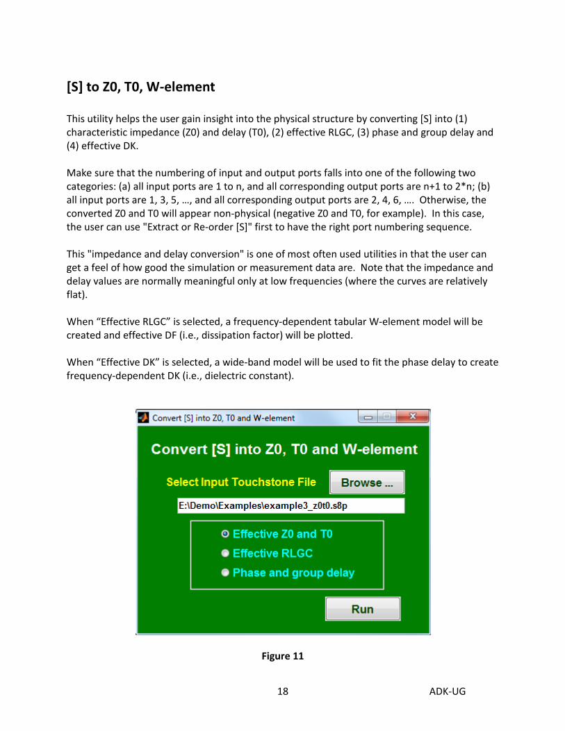
[S] to Z0, T0, W-element This utility helps the user gain insight into the physical structure by converting [S] into (1) characteristic impedance (Z0) and delay (T0), (2) effective RLGC, (3) phase and group delay and (4) effective DK. Make sure that the numbering of input and output ports falls into one of the following two categories: (a) all input ports are 1 to n, and all corresponding output ports are n+1 to 2*n; (b) all input ports are 1, 3, 5, …, and all corresponding output ports are 2, 4, 6, …. Otherwise, the converted Z0 and T0 will appear non-physical (negative Z0 and T0, for example). In this case, the user can use "Extract or Re-order [S]" first to have the right port numbering sequence. This "impedance and delay conversion" is one of most often used utilities in that the user can get a feel of how good the simulation or measurement data are. Note that the impedance and delay values are normally meaningful only at low frequencies (where the curves are relatively flat). When “Effective RLGC” is selected, a frequency-dependent tabular W-element model will be created and effective DF (i.e., dissipation factor) will be plotted. When “Effective DK” is selected, a wide-band model will be used to fit the phase delay to create frequency-dependent DK (i.e., dielectric constant).

Figure 11

ADK-UG 19

Figure 12

Figure 13

region of interest

ADK-UG 20

Change Impedance This utility allows the user to (1) change [S] to different reference impedance, (2) scale the impedance and/or length of [S] ( - think TDR/TDT), (3) output Touchstone files in different format, (4) plot S/Y/Z in log(f) and (5) save in a .csv file for Excel. In this example (Figure 14 to Figure 15), we scale the impedance of Touchstone file: example3.s8p_passivity.s8p up by 1.1x, and create a new Touchstone file: example3.s8p_passivity.s8p_scale.s8p. This type of "impedance scaling" has been found useful in correcting results from 3D full-wave solvers. In other applications, the user may simply want to convert the Touchstone file to different reference impedance. Then, he/she can set "Impedance Scaling" to 1, and vary the "Output Reference Impedance". Optionally, the user can also scale the “length” for the Touchstone file. Effectively, all frequencies are divided by the “length scaling factor”. If the original Touchstone file has [S] from 0 to 20 GHz, and a length scaling factor of 2 is entered, the new Touchstone file will contain the same [S] from 0 to 10 GHz.

ADK-UG 21

Figure 14

Figure 15

Before

After

ADK-UG 22

TDR and TDT This utility allows [S] to be converted into impedance profile, TDR with open end, or TDR/TDT with matched terminations. The user can select step, single-bit or impulse response. (The impulse response corresponds to the derivative of step response with zero rise time.) Zero is assumed for [S] above the Touchstone file bandwidth. When step or single-bit response is selected, the input waveform before filter is assumed to be trapezoidal. With the default of 41.4448ps input rise time (20% to 80%), Butterworth filter with 6.3337GHz bandwidth (=0.35/(10% to 90% rise time)), and -20 dB/dec roll-off, the 20% to 80% rise time of output waveform will be 50ps with 1000GHz bandwidth and 50.0293ps with 20GHz bandwidth. When “TDR & TDT with Matched Termination” is selected, the filter output waveform (VIN) with the same Touchstone file bandwidth is plotted, together with a summary of rise time, delay, skew and maximum crosstalk amplitude, etc. The user has the option of applying TDR/TDT to single-ended, differential-mode or common-mode signals. Two types of port sequence are supported for differential- or common-mode signals: (1) 1 to N as inputs and N+1 to 2N as outputs (which is preferred) and (2) 1, 3, …, 2N-1 as inputs and 2, 4, …, 2N as outputs. See Figure 21 for details about how the differential pairs are numbered. To reveal non-causal behavior, if any, all waveforms are plotted starting at -1 ns. Responses before time x (with x>=0) can be indication of non-causality. The user has the option of adding delay to shift the waveform and observe responses before -1 ns. By default, all curves for TDR/TDT will be plotted (Figure 16 and Figure 17). The user can select an individual curve to plot (Figure 18 and Figure 19). See Figure 21 and Table 3 for valid port indices.

ADK-UG 23

Figure 16

Figure 17

ADK-UG 24

Figure 18

Figure 19

ADK-UG 25

Single to Mixed-Mode With this utility (Figure 20), we can convert single-ended [S] into mixed-mode [S]. Three choices are available. In this example, a .s8p file is converted into a .s4p file if "Diff Mode Only" or “Common Mode Only” is selected. If “Mixed Mode” is selected, a single-ended .s8p file will be converted into an odd-and-even mixed-mode .s8p file with one single reference impedance. The user may note that the odd-mode S parameters with reference to Z are identical to differential-mode S parameters with reference to 2Z, and the even-mode S parameters with reference to Z are identical to common-mode S parameters with reference to Z/2. So, the user can view the differential- and common-mode S parameters directly by viewing the odd- and even-mode S parameters. By default, the program will automatically identify point-to-point connection and assign suitable differential pairs. To override, the user can select one of two differential pair orders. As shown in Figure 21, the output mixed-mode matrix always assumes SDD at the upper left-hand corner and SCC at the lower right-hand corner. Regardless of the single-ended port sequence, the differential pairs are assigned to the input ports first.

Wildcard character

To process many files at the same time, a wildcard character (*) can be used. For example, if "D:\demo\ab*cd.s*p" is specified as input file, the program will look for all files with "*" replaced by any character(s).

ADK-UG 26

Figure 20

ADK-UG 27

Figure 21

ADK-UG 28

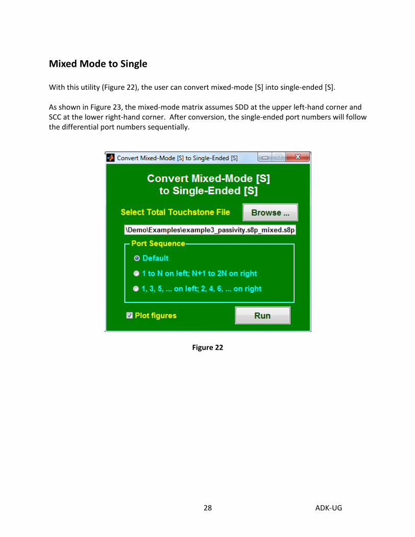
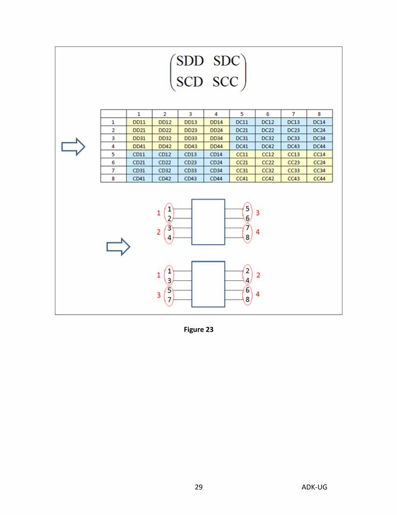
Mixed Mode to Single With this utility (Figure 22), the user can convert mixed-mode [S] into single-ended [S]. As shown in Figure 23, the mixed-mode matrix assumes SDD at the upper left-hand corner and SCC at the lower right-hand corner. After conversion, the single-ended port numbers will follow the differential port numbers sequentially.

Figure 22

ADK-UG 29

Figure 23

ADK-UG 30

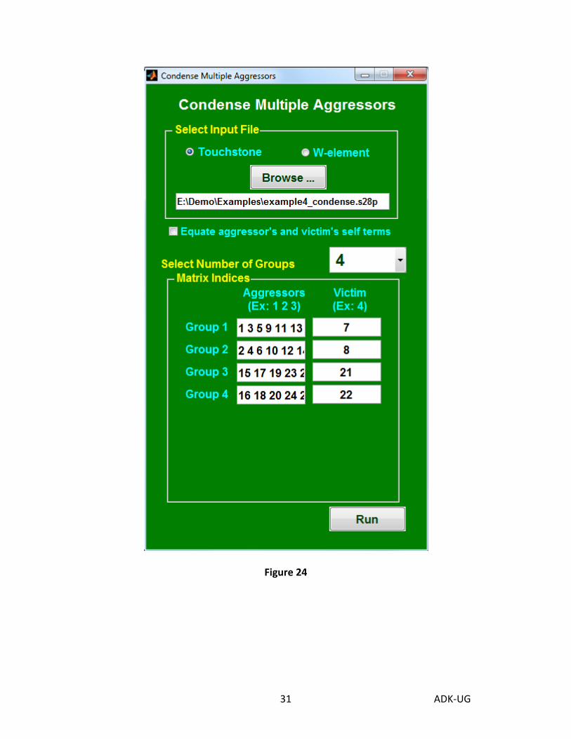
Condense Aggressors With this utility, the user can combine multiple aggressors and reduce the total number of ports. It allows the user to simulate the "worst-case" coupling more efficiently in SPICE, for example. All port numbers in each group of aggressors are entered with "space" as separator (Figure 24). The newly generated Touchstone file follows the port sequence of smallest port indices in each aggressor and victim group (Table 2 in this example). To check, the user can use "Find Port Connection". Optionally, the aggressor's self terms (insertion and return losses, and coupling, if more than 2 ports) are replaced by the victim's. In this example with the new Touchstone file, Port 3, 4, 7, 8 will see the same response as Port 1, 2, 5, 6, respectively. In addition to Touchstone files, the user can condense W-element files. Effectively all aggressor transmission lines are placed in parallel. The final RLGC matrices have the combined coupling, with the aggressor's self terms replaced by the victim's.

Old Port Indices New Port Indices 1 1 2 2 7 3 8 4

15 5 16 6 21 7 22 8

Table 2

ADK-UG 31

Figure 24

ADK-UG 32

Plot Multiple Curves With this utility (Figure 25), the user can import multiple Touchstone files (in .s*p) or time-domain files (in .out), select S-parameter indices, and plot S, Y, Z parameters, equivalent inductance (L), vswr or time-domain curves on the same graph. In addition, the user can import multiple .csv files, select proper column from each file and plot them on the same graph. (Note that only files of the same format can be plotted together.) Table 3 gives an example of various indices that can be entered to plot single-ended, mixed-mode, and single-ended vs. mixed mode responses.

Valid indices Remarks

.snp

3 4 Sgl to Sgl Port 4 to Port 3 3, 4 are port # dd 3 4 d 3 d 4 D to D Pair 4 to Pair 3 3, 4 are pair # dc 3 4 d 3 c 4 C to D Pair 4 to Pair 3 3, 4 are pair # cd 3 4 c 3 d 4 D to C Pair 4 to Pair 3 3, 4 are pair # cc 3 4 c 3 c 4 C to C Pair 4 to Pair 3 3, 4 are pair # dd 5 6 7 8 d 5 6 d 7 8 D to D Pair (7,8) to Pair (5,6) 5, 6, 7, 8 are port # dc 5 6 7 8 d 5 6 c 7 8 C to D Pair (7,8) to Pair (5,6) 5, 6, 7, 8 are port # cd 5 6 7 8 c 5 6 d 7 8 D to C Pair (7,8) to Pair (5,6) 5, 6, 7, 8 are port # cc 5 6 7 8 c 5 6 c 7 8 C to C Pair (7,8) to Pair (5,6) 5, 6, 7, 8 are port # sd 3 5 6 s 3 d 5 6 D to Sgl Pair (5,6) to 3 3, 5, 6 are port # ds 5 6 3 d 5 6 s 3 Sgl to D 3 to Pair (5,6) 3, 5, 6 are port # sc 3 5 6 s 3 c 5 6 C to Sgl Pair (5,6) to 3 3, 5, 6 are port # cs 5 6 3 c 5 6 s 3 Sgl to C 3 to Pair (5,6) 3, 5, 6 are port #

.out 3 4 Sgl to Sgl Port 4 to Port 3 3, 4 are port #

.csv 3 3 is column #

Table 3 To summarize:

1. The row and column indices are separated by space (for example: “3 4”). 2. To plot mixed-mode S, Y, or Z parameters, the user can enter the differential pair indices

with preceding “d” or “c” (for example: “dd 3 4”, “dc 3 4”, “cd 3 4”, “cc 3 4”, “d3 d4”, “d3 c4”, “c3 d4”, or “c3 c4”, etc.). The program will figure out the correct mixed modes as long as the single-ended ports are in one of two ordering sequences: (1) Ports 1 to N are inputs and Ports N+1 to 2*N are outputs, or (2) Ports 1, 3, 5, … are inputs and Ports 2, 4, 6, … are outputs. See Figure 21 for the mixed-mode indices after conversion.

3. An alternate way to plot mixed-mode S, Y, or Z parameters is to enter the single-ended port indices directly for each differential pair. For example, if Ports 5 & 6 form a pair

ADK-UG 33

and Ports 7 & 8 form another pair, the user can enter: “dd 5 6 7 8”, “dc 5 6 7 8”, “cd 5 6 7 8”, “cc 5 6 7 8”, “d 5 6 d 7 8”, “d 5 6 c 7 8”, “c 5 6 d 7 8”, or “c 5 6 c 7 8”.

4. To plot single-ended vs. mixed mode S, Y, or Z parameters, the user can enter the single-ended port indices preceded by “s”, “d”, or “c”. For example, if Ports 5 & 6 form a pair and Port 3 is a separate single-ended port, the user can enter: “sd 3 5 6”, “ds 5 6 3”, “sc 3 5 6”, “cs 5 6 3”, “s 3 d 5 6”, “d 5 6 s 3”, “s 3 c 5 6”, or “c 5 6 s 3”.

5. Useful for EMC application, equivalent inductance (L) is computed by converting S into Z and equating Z to R+jwL.

6. Selecting "Smith" plots the Smith chart: the x axis is the real part of S parameter and the y axis is the imagnary part of S parameter. In this case, Figure Property is disabled except for Xsize, Ysize, Legend and Line Color. See the Figure Property section below.

7. Checking "Delay/DK" plots phase delay or DK values (if length in inch is specified). Length for DK plot can be entered in either a single number or a vector of multiple numbers separated by space (such as "2" or "2 1 1.5"). If phase delay is chosen and only two curves are specified, skew will be displayed on the screen.

8. No “s”, “d”, or “c” prefix is allowed to plot .out files. To plot mixed-mode time-domain responses, the user can convert the single-ended S-param into mix-mode S-param (thru the “Single to Mixed-Mode” utility) before applying TDR/TDT. Then, the .out files will contain mixed-mode responses, and the user just needs to specify the correct indices (see below).

9. Another alternate (though unnecessary) way to plot mixed-mode response is to create a Touchstone file through “Single to Mixed-Mode” utility and plot the corresponding indices. (For example, the user can enter the indices of “2 6” for the mixed-mode file of Figure 21 to plot SDC22.) To be consistent throughout ADK, it’s a good practice to number the input ports from 1 to N and the output ports from N+1 to 2*N. The mixed-mode matrix always assumes SDD at the upper left-hand corner and SCC at the lower right-hand corner:

[ ]

=

CCCD

DCDDmixed SS

SSS

Figure Property

By default, the figure properties are left as blank and the program automatically plots the entire x and y ranges. The user has the option to enter a specific x, y range to plot and override the default label, legend, line color and line width, etc. Valid line colors are in b (blue), r (red), k (black), m (magenta), c (cyan), g (green), y (yellow). The default of "brkmcg" corresponds to that the 1st curve is in blue and the 2nd curve is in red, etc. Certain publications (such as patent, journal, …) require that all graphs be in black and white. The user can just enter "k" in this case and the program will plot all curves in black with solid line, dashed line, …, etc.

ADK-UG 34

The user can enter a math expression in Matlab format with variables: freq for frequency and s1, s2, … for the value of the 1st, 2nd, … curve, etc. Multiple math equations can be entered, separated by semi-colons (";"). When a math expression is entered, an output file: XXX_math.csv, with XXX being the first input file name, is created. The user can import that .csv file back, enter proper column numbers and re-plot the graph.

Reset reference impedance

The user can change reference impedance for all ports by entering either a single number or multiple numbers. Through multiple numbers (in such a vector form as "42.5 45 50 …"), the reference impedance for each port can be specified differently.

Correlation

When only two curves are plotted, “Correlation”, as defined below, is computed and displayed on the screen.

𝑐𝑜𝑟𝑟𝑒𝑙𝑎𝑡𝑖𝑜𝑛 = 1 − 2 ×∫|𝑆1(𝑓) − 𝑆2(𝑓)|2𝑑𝑓

∫|𝑆1(𝑓)|2𝑑𝑓 + ∫|𝑆2(𝑓)|2𝑑𝑓

Both frequency- and time-domain curves are supported.

ADK-UG 35

Figure 25

ADK-UG 36

(a)

(b)

Figure 26

ADK-UG 37

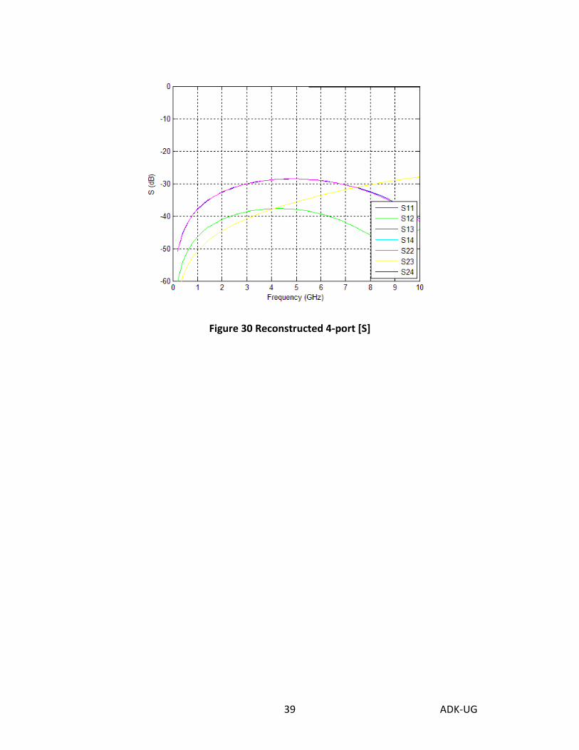
Combine PEC and PMC With this utility, the user can reconstruct the [S] matrix of a symmetric structure by importing two [S] matrices of half the original structure with the symmetry plane replaced by perfect electric conductor (PEC) and perfect magnetic conductor (PMC), respectively. If there exist two symmetry planes, the user can invoke this utility three times, using 4 sets of Touchstone files: [See], [Sem], [Sme], [Smm], where e and m denote PEC and PMC in each symmetry plane. In the first run, the user combines [See] and [Sem] into [Se]. In the second run, the user combines [Sme] and [Smm] into [Sm]. In the third run, the user combines [Se] and [Sm] into [S]. Combining this utility with a field solver (such as HFSS), the user can find more than 2x CPU time reduction in simulating a structure with one symmetry plane, and more than 4x CPU time reduction in simulating a structure with two symmetry planes, etc.

Figure 27

ADK-UG 38

Figure 28 2-port [S] with PEC

Figure 29 2-port [S] with PMC

ADK-UG 39

Figure 30 Reconstructed 4-port [S]

ADK-UG 40

RLGC to [S] With this utility, the user can import coupled transmission lines in W-element file format (Table 4), enter the length and frequency range, and create a Touchstone file. It helps engineers study the insertion loss, return loss, near-end crosstalk (NEXT), and far-end crosstalk (FEXT) of transmission lines at any frequency. The user can pre-process (“ground”, “float”, “group” and “group & float”) the W-element file by specifying conductor indices separated by space. Semicolons (;) are used to separate groups of conductors in “group” and “group & float”. Effectively, “ground” enforces the conductor voltage to be 0, “float” enforces the conductor current to be 0, “group” enforces a group of conductors to be at the same voltage and “group & float” enforces a group of conductors to be at the same voltage before they are floated together. In this example (Figure 31), 14x14 RLGC matrices are reduced to 4x4 RLGC matrices and a new W-element file (ustrip_14lines.rlc_new.rlc) is created before S parameters are generated. The user can also select among causal, non-causal and roughness models to generate S parameters. In this example, in addition to ustrip_14lines.rlc_new.rlc, new files are created, depending on the model that is selected:

Causal -> ustrip_14lines.rlc_causal.s8p ustrip_14lines.rlc_causal.tbl

Non-causal -> ustrip_14lines.rlc_noncausal.s8p

Roughness -> ustrip_14lines.rlc_rough.s8p

ustrip_14lines.rlc_rough.tbl ustrip_14lines.rlc_rough.rlc

The frequency-dependent W-element models (in .tbl) help the user study frequency-dependent RLGC in more details. When the roughness model is selected, a new panel (Figure 32) is displayed, prompting the user to enter the desired insertion loss at two frequencies. The program will then (1) adjust Rs and Gd to fit the insertion loss and (2) adjust frequency-dependent Gd and C0 to fit a causal wideband model (ustrip_14lines.rlc_rough.tbl) and (3) create a Touchstone file (ustrip_14lines.rlc_rough.s8p). For reference, a simple non-causal W-element model (ustrip_14lines.rlc_rough.rlc) is also outputted.

ADK-UG 41

Figure 31

* No. of lines 14 * Lo 2.965041e-07 4.142613e-08 2.945722e-07 1.169020e-08 4.094198e-08 2.944213e-07 : * Co 9.848361e-11 -5.260869e-12 9.888336e-11 -6.117512e-13 -5.201307e-12 9.889183e-11 :

Table 4

ADK-UG 42

* No. of lines 4 * Lo 2.959984e-07 3.973082e-08 2.887619e-07 1.004299e-09 1.125566e-09 1.668722e-07 6.591310e-10 6.804841e-10 1.704956e-08 1.662995e-07 * Co 9.848331e-11 -5.261371e-12 9.888253e-11 -1.106622e-13 -1.505276e-13 1.870441e-10 -5.791703e-14 -7.269244e-14 -6.652536e-12 1.871574e-10 * Ro 2.227016e+00 0.000000e+00 2.227016e+00 0.000000e+00 0.000000e+00 1.113508e+00 0.000000e+00 0.000000e+00 0.000000e+00 1.113508e+00 * Go 0.000000e+00 0.000000e+00 0.000000e+00 0.000000e+00 0.000000e+00 0.000000e+00 0.000000e+00 0.000000e+00 0.000000e+00 0.000000e+00 * Rs 1.160627e-03 1.443745e-04 1.152461e-03 6.649509e-06 7.636781e-06 6.611505e-04 4.585606e-06 4.835392e-06 7.340580e-05 6.597739e-04 * Gd 7.488949e-12 -4.512674e-14 7.455745e-12 2.580537e-15 2.338687e-15 1.481405e-11 2.180607e-15 1.880182e-15 -3.645718e-14 1.481432e-11 * Original index New index * ------------------------------------------ * 1 1 * 2 2 * 3 ground * 4 ground * 5 float * 6 float * 7 3 * 8 3 * 9 4

ADK-UG 43

* 10 4 * 11 float (with 11 original) * 12 float (with 11 original) * 13 float (with 13 original) * 14 float (with 13 original)

Table 5

Figure 32

ADK-UG 44

Cascade [S] With this utility, the user can easily cascade [S] when all Touchstone files have the same number of ports. Two choices of port sequence are available: (1) all input ports are numbered from 1 to N and output ports are numbered from N+1 to 2*N and (2) all input ports are odd-numbered and all output ports are even-numbered. The user also has the option to pad ideal transmission lines, change output reference impedance and specify new Touchstone file name. For arbitrary circuit connection, the utility: "Convert SPICE circuit into [S]" can be used.

ADK-UG 45

Figure 33

ADK-UG 46

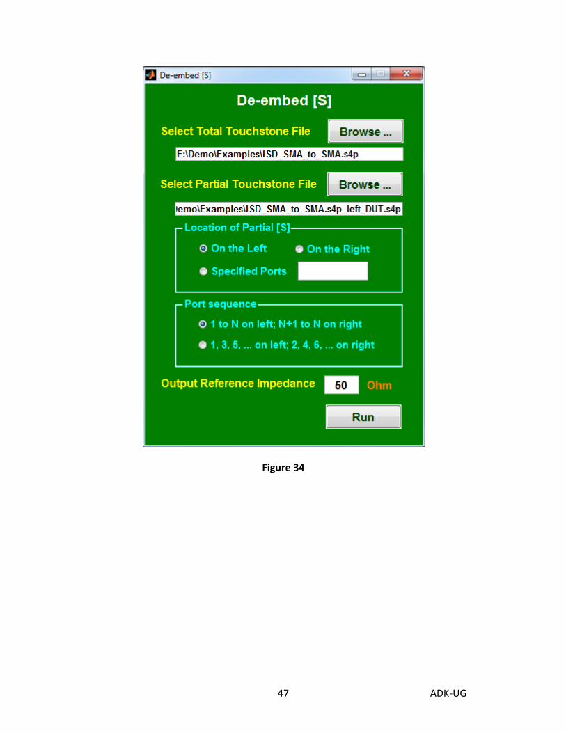
De-embed [S] With this utility, the user can easily de-embed partial [S] from total [S]. Three choices for the location of partial [S] are available (see Figure 35): (1) the partial [S] is on the left side of total [S], (2) the partial [S] is on the right side of total [S], and (3) the partial [S] is at arbitrary location relative to the total [S]. For the first two selections, both partial and total [S] must have the same (even) number of ports with either Ports 1 to N as inputs and Ports N+1 to 2*N as outputs or Ports 1, 3, 5, … as inputs and Ports 2, 4, 6, …. as outputs. For the third selection, the partial [S] must have even number of ports with either Ports 1 to N as inputs and Ports N+1 to 2*N as outputs or Ports 1, 3, 5, … as inputs and Ports 2, 4, 6, … as outputs. The total [S] can have either odd or even number of ports, but the total number of ports must be larger than one half of the total number of ports in partial [S]. In the example of Figure 35, the output ports of partial [S] are connected to Ports 2 and 3 of DUT. The user will select “Specified Ports” and enter “2 3” (i.e., port numbers separated by space) to de-embed partial [S].

ADK-UG 47

Figure 34

ADK-UG 48

Figure 35

ADK-UG 49

Combine [S] With this utility, the user can combine several Touchstone files and expand it into a file with more ports. Zeros are inserted for un-specified [S]. One application is to combine many 4-port measurement files into a larger multi-port file. All Touchstone files will be synced automatically to the first file for the same frequencies and reference impedance. Two methods are available: “Combine by [S]” and “Combine by [Z]”. The user should choose “Combine by [S]” if the un-measured ports are terminated and “Combine by [Z]” if the un-measured ports are open. The following example shows how to combine six .s4p files into a complete .s8p file. Ports 1 to 4 are inputs and Ports 5 to 8 are outputs. The port sequence for six measurements is:

1-2-3-4 (NEXT) 1-2-7-8 (FEXT) 3-4-5-6 (NEXT) 5-6-7-8 (NEXT) 1-2-5-6 (THRU) 3-4-7-8 (THRU)

Note that when there are duplicate port numbers, the data from the file specified later will override the data from the file specified earlier. For more accurate return loss, it’s usually a good idea to specify the file that contains the thru measurement (i.e., insertion loss) last. To skip certain ports from a Touchstone file for combination, the user can assign to those ports a port number that is larger than the “total number of ports after combination”. Then, those “unwanted” ports will be dropped after combination. “Reset Configuration” in the menu bar presets the port sequence and guides the user to combine six .s4p files into one .s8p file.

ADK-UG 50

Figure 36

ADK-UG 51

Merge [S] With this utility, the user can merge several Touchstone files with data at different frequencies. One application is to combine Ansys's HFSS outputs after running several different "sweeps".

Figure 37

ADK-UG 52

Change Reference Port By default, a Touchstone file uses a common ground reference. There are situations that the user wants to use a separate reference port for each input port (or each group of input ports). If all ports are assigned to group(s), the “original” ground reference will be floated. A practical application can be found in making the boundary of waveguide port a temporary reference for HFSS simulations, and then changing the reference to complex ground structures during post-processing.

Figure 38

ADK-UG 53

[S] to SPICE With this tool, the user can convert [S] into equivalent SPICE circuit models. S-to-SPICE is particularly useful for those users who want to simulate [S] in SPICE, but their SPICE simulator does not handle [S] properly. After clicking the “[S] to SPICE” button, the user will see a window (Figure 39) where they can import a Touchstone file, select the number of poles to rationally fit the S parameters, create a new Touchstone file and optionally turn on/off figure plotting. Additional run controls are available to enforce reciprocity and passivity and/or to match DC values after fitting. If the input Touchstone file does not contain DC values and the “Match DC Values” button is enabled, extrapolated DC values will be used. The user is advised to use ADK’s utility: "Passivity and Causality” function to fill in correct DC values. After the “Run” button is pressed, S-to-SPICE will create an output file (under the name of InputFileName.spi) that contains equivalent SPICE models. An example of such output file is shown in Table 6 where n1 to n8 correspond to Port 1 to Port 8 and Lgnd is the ground node. If “Plot figures” is enabled, the fitted S parameters will be plotted to 2x the original maximum frequency by default (unless overridden by “Maximum Frequency” in “Create New Touchstone File Using Fitted Curves”). Plotting fitted S parameters beyond the original maximum frequency allows the user to get a feel of how the fitted model behaves outside the original frequency range. To compare S parameters before and after conversion more closely, the user can enable "Create New Touchstone File Using Fitted Curves", and invoke ADK’s utility: "Plot Multiple Curves” to plot multiple curves on the same graph.

ADK-UG 54

Figure 39

.subckt AtaiTec n1 n2 n3 n4 n5 n6 n7 n8 Lgnd V_1 n1 n1x 0 R_1 n1x n1y 50 H_1 n1y Lgnd V_b1 14.1421 V_2 n2 n2x 0 R_2 n2x n2y 50 H_2 n2y Lgnd V_b2 14.1421

:

.ends AtaiTec

Table 6

ADK-UG 55

Figure 40

ADK-UG 56

SPICE to [S] With this utility, the user can easily convert a SPICE-like circuit into [S]. The input file assumes the following format (Table 7): 1. The header starts with '.subckt' followed by the sub-circuit name and output node names.

The last node is assumed to be ground. A Touchstone file will be created following the sequence of output node names (except the last node).

2. Each statement must be completed in one line. No continuation is allowed. 3. The syntax of each statement is in the form of

R1 A B 10 L2A 1 2 2e-9 C3B X1 Y2 3e-12 K12 L1 L2 0.1 SXX I1 I2 O1 O2 filename

where the first character: R, L, C, K, S indicates whether the statement is for resistance, inductance, capacitance, inductive coupling, or S parameters. In the last entry, only pure numeric values (without such units as pF, nH, …) are allowed for R, L, C, and K; and a Touchstone file name is specified for S. Between the first and last entries, arbitrary alphanumeric node names can be used.

4. The node name '0' is assumed to be ground. 5. All variable names are case insensitive. 6. Blank lines or comment statements (that start with '*') are ignored. 7. A '.ends' statement is always used at the end of circuit description.

ADK-UG 57

Figure 41

.subckt via_conn_via i1 i2 i3 i4 …. 8 o9 o10 o11 o12 o13 o14 gnd0 svia a1 a2 a3 a4 a5 a6 a7 a8 … i13 i14 C:\ADK\examples\via.s28p scon a1 a2 a3 a4 … b10 b11 b12 b13 b14 C:\ADK\examples\conn.s28p svia b11 b12 b13 … o8 o9 o10 o1 o2 o3 o4 C:\ADK\examples\via.s28p .ends via_conn_via

Table 7

ADK-UG 58

Scope to Spectrum With this utility, the user can plot waveforms, eye diagrams or spectra from scope measurement data, tabular data, HSPICE .tr0 files or ADS .mdf files. In addition, the user can perform de-embedding and/or embedding on the above data. The default input file extensions are in .csv, .txt, .out, .tr0 and .mdf.

Scope measurement data (.csv and .txt)

The scope measurement data, with the default file extension of .csv and .txt, are accepted as inputs in three different file formats: WaveformPattern, WaveformYValues and WaveformXYValues. Table 8 to Table 10 show some examples of such file formats. After importing the data, the user can select waveform, eye diagram or spectrum to plot. In this example (Figure 42 to Figure 43), the waveform corresponds to a periodic PRBS7 pattern at 25.78125 Gbps, though it contains more than 127 bits. To see the entire waveform, we enter PRBS20 and the program will display up to the available bits. In Figure 44 to Figure 45, we take a time window of the above waveform and plot a 2-bit eye diagram with eye masks. PRBS7 is now used and the waveform of first 30.1607 ps is being skipped in order to center the eye. (The suggested delay to center the eye, eye height and eye width are echoed to the screen and also saved in a log file: <input_file_name>.log.) Multiple eye masks can be specified with vectors of “x y” pairs separated by semicolon (;). In Figure 44, “10 0 20 0.02 30 0 20 -0.02 10 0; 50 0 60 0.02 70 0 60 -0.02 50 0” was entered. The spectrum of the above PRBS7 pattern, which is assumed to be periodic, is shown in Figure 46 to Figure 47. The user may notice a null at 25.78125 GHz, which corresponds to the data rate (or 2x the fundamental frequency). The total period is 4.9261 ns ( = 127/25.78125e9), so the spectrum is plotted at 0.203 GHz ( = 1/4.9261e-9) interval. Because the # of samples per bit is 10, the maximum frequency one can plot will be 128.91 GHz ( = 1/(2*(1/25.78125e9)/10).

Tabular data (.out)

Tabular data in the form of time and voltage can be imported (see Table 11). The operation is similar to what is described in “Scope measurement data”. An example is shown in Figure 48 to Figure 49.

HSPICE .tr0 files

ADK-UG 59

The HSPICE .tr0 files must be in text format. To create a .tr0 file in text format, the user can add ".option csdf" (for Viewlogic's Common Simulation Data Format) to their HSPICE deck before simulation. The user can click "List …" to show the available variable names in a .tr0 file. Entering the data rate of 6.25 Gbps and delay of 17.374 ps in this example (Figure 50) places the eye crossing the center (Figure 51). Multiple threshold voltages can be specified in a vector form (“0 0.1” in Figure 50) to measure different eye widths at the corresponding voltages. The output file (example11.tr0.log as shown in Table 12) lists the eye height, eye width and suggested delay, etc. The rest of operation is similar to what is described in “Scope measurement data”.

ADS .mdf files

The ADS .mdf file format resembles tabular data with header (Table 13). The user can click "List …" to show the available variable names in an .mdf file. The operation is similar to what is described in “HSPICE .tr0 files”.

De-embedding and embedding

The user can easily de-embed or embed an S-param block (in .s2p or .s4p) from the above time-domain data. When a .s4p file is used, the program will internally convert it into a differential .s2p file. Figure 52 to Figure 53 show a bigger eye than Figure 48 to Figure 49 after a trace is de-embedded. Note that de-embedding and embedding the same file does not get back to the original waveform because de-embedding in this context effectively places a high-impedance probe in front of the S-param block rather than removes the S-param block from the channel.

ADK-UG 60

File Format, WaveformPattern Format Version, 1 Instrument, 86100D SwVersion, A.03.01.5 SerialNumber, MY53060153 Date, 08/02/2014 11:14:27 SourceName, CTLE[D1A] Points, 4064 XOrg, 2.40002580545526E-08 XInc, 1.21212121212121E-12 Bit Rate (b/s), 25781250000 Points/Bit, 32 Pattern Length, 127 X Units, Second Y Units, Volt Data, -0.0972043574277879 -0.0980490695429733

Table 8

File Format, WaveformYValues Format Version, 1 Instrument, 86100D SwVersion, A.03.01.5 SerialNumber, MY53060153 Date, 08/02/2014 11:10:24 SourceName, DFE[F1] Points, 9277 XOrg, 2.42545454545455E-08 XInc, 1.21212121212121E-12 X Units, Second Y Units, Volt Data, -0.0748313216372917 -0.0737548155495842 -0.0728663540076539

Table 9

ADK-UG 61

File Format, WaveformXYValues Format Version, 1 Instrument, 86100D SwVersion, A.03.01.5 SerialNumber, MY53060153 Date, 08/02/2014 10:39:18 SourceName, Differential 1A Points, 8251 X Units, Second Y Units, Volt Data, 2.400755E-08, -0.146654043158611 2.40087621212121E-08, -0.151440414809714 2.40099742424242E-08, -0.152424544124795 2.40111863636364E-08, -0.150073492591298 2.40123984848485E-08, -0.150932909448926 2.40136106060606E-08, -0.152173535800706 2.40148227272727E-08, -0.15194047639801

Table 10

2.400755E-08 -0.146654043158611 2.40087621212121E-08 -0.151440414809714 2.40099742424242E-08 -0.152424544124795 2.40111863636364E-08 -0.150073492591298 2.40123984848485E-08 -0.150932909448926 2.40136106060606E-08 -0.152173535800706 2.40148227272727E-08 -0.15194047639801 2.40160348484849E-08 -0.152857220794053 2.4017246969697E-08 -0.154601631701206 2.40184590909091E-08 -0.149134225888913 2.40196712121212E-08 -0.154363166888618 2.40208833333333E-08 -0.151480579826525 2.40220954545455E-08 -0.153257358212384 2.40233075757576E-08 -0.147140733093904 2.40245196969697E-08 -0.14875042498045 2.40257318181818E-08 -0.152091190098932

Table 11

ADK-UG 62

Figure 42

Figure 43

ADK-UG 63

Figure 44

Figure 45

ADK-UG 64

Figure 46

Figure 47

ADK-UG 65

Figure 48

Figure 49

ADK-UG 66

Figure 50

Figure 51

ADK-UG 67

Variable Selected: V(RX_INPA,RX_INNA) ----- Inputs ----- Input file = E:\Demo\Examples\example11.tr0 Data rate = 6.25 Gbps ----- Outputs ----- *** Threshold voltage = 0 volt Eye height = 0.443558 volt Eye width = 124.44 ps Jitter = 35.5602 ps Skip waveform to center eye = 17.374 ps *** Threshold voltage = 0.1 volt Eye height = 0.443558 volt Eye width = 93.3717 ps Jitter = 66.6283 ps Skip waveform to center eye = 19.022 ps

Table 12

! Created Thu Aug 28 12:19:37 2014 BEGIN Tran1.TRAN % time(real) Vout1(real) Vout2(real) tranorder(real) 1.0000000E-09 1.7202248E-07 -1.7168385E-07 2 1.0001966E-09 1.7223009E-07 -1.7189055E-07 2 1.0006966E-09 1.7276001E-07 -1.7241724E-07 2 1.0011966E-09 1.7329245E-07 -1.7294646E-07 2 1.0016966E-09 1.7382771E-07 -1.7347807E-07 2 1.0021966E-09 1.7436484E-07 -1.7401209E-07 2 1.0026966E-09 1.7490512E-07 -1.7454864E-07 2 1.0031966E-09 1.7544759E-07 -1.7508768E-07 2

Table 13

ADK-UG 68

Figure 52

Figure 53

ADK-UG 69

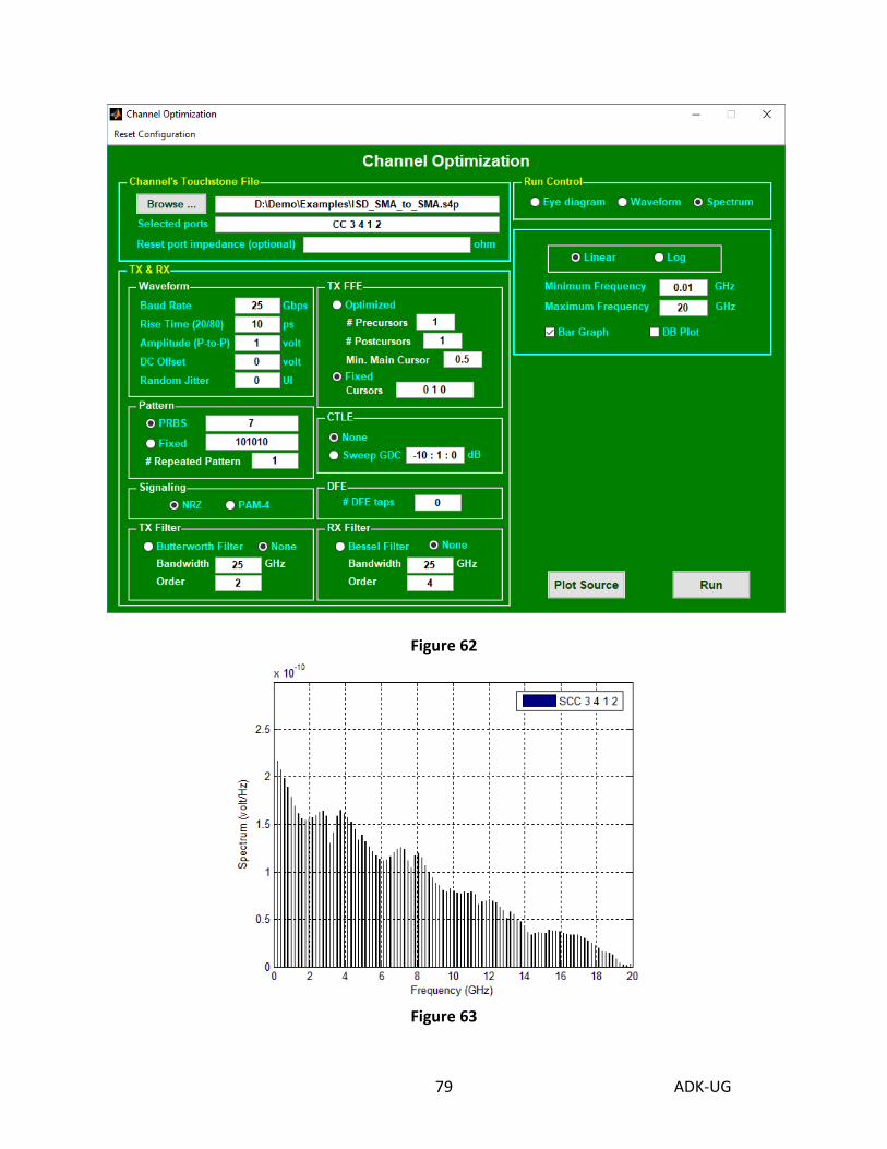
Channel Optimization With this utility, the user can easily import S parameters, select single-ended or mixed-mode IL, RL, NEXT and FEXT, run bit-by-bit simulation for NRZ or PAM-4 signals and plot waveform, eye diagram or spectrum with PRBS or fixed data pattern and TX FFE, RX CTLE and RX DFE tap coefficients.

Inputs and outputs

In Figure 54, we import a .s4p file, select ports: “DD 3 4 1 2” (for differential insertion loss from Ports 1 & 2 to Ports 3 & 4 – see Table 3 in “Plot Multiple Curves” for detailed description), select optimized TX tap coefficients with 1 pre- and 1 post-cursor and plot a 2-bit eye (Figure 55). The optimized tap coefficients, eye height, eye width and jitter are displayed on the screen (Figure 56). In addition, an output .log file (ISD_SMA_to_SMA.s4p.log in this case, also shown in Table 14) that contains pertinent information is saved in the same directory as the input file.

Selected ports

Multiple S parameters can be summed together, with their respective port indices separated by semicolon (;). In Figure 57 to Figure 58, we simulate the single-ended transmission (S31) with NEXT (S34) and FEXT (S32) included.

Random Jitter and Reference BER

Random jitter, specified in unit interval (UI), is used in conjunction with reference BER. When non-zero random jitter (σrms) is entered, the eye diagram will be shifted by ±Q·σrms where

𝑄 = √2 ∙ 𝑒𝑟𝑓𝑐−1(2 ∙ 𝐵𝐸𝑅)

Random jitter must be between 0 and 0.1; BER must be between 1e-40 and 0.1

TX tap coefficients

The user can select either optimized or fixed TX tap coefficients. When fixed TX tap coefficients are selected, the cursors are entered in a vector (such as “-0.02 -0.03 0.85 -0.08 -0.02”) where

• The main cursor takes on the largest value of input vector.

ADK-UG 70

• The pre- and post-cursors are the numbers before and after the main cursor, respectively.

• Any number of pre- and post-cursors can be specified.

Continuous time linear equalization (CTLE)

The transfer function of CTLE is defined by

( ) ( ) ( )bb

G

bbCTLE ffjffj

ffjffH

DC

+⋅⋅⋅+⋅⋅⋅+⋅

⋅=25.0

1025.0 20

where fb is the baud rate (or data rate in the “Channel Optimization” window) and GDC is the DC gain (in dB) which, using the syntax of -10:1:0, for example, is swept from -10 to 0 dB in 1 dB increment.

Decision feedback equalizer (DFE)

The DFE output, y(t), is defined by

( ) ( ) ( )bd

N

ni nTtywtxty −⋅+= ∑

=1

where x(t) is the receiver input, wi’s are the DFE tap coefficients, Tb is the bit time and yd (=1 or -1) is the slicer’s output. DFE is turned off when # DFE taps is set to 0.

TX filter

A TX Butterworth filter can be specified, with transfer function H(f) given by

=

cffjG

fH

1)(

where

ADK-UG 71

( )

=

+

−+

⋅−

=

+

−+

⋅−⋅+=

∏

∏

=

−

=

n

k

n

k

nnkss

nnksss

sG

1

2

21

1

2

evenn 12

12 cos2

oddn 12

12 cos21)(

π

π

and n is order, fc is bandwidth. It can be shown that

n

cff

fH2

1

1)(

+

=

RX filter

An RX Bessel-Thomson filter can be specified, with transfer function H(f) given by

=

cffjG

GfH

)0()(

where ( )

( )k

n

kkn s

knkknsG

! ! 2! 2)(

0∑=

− −−

=

and n is order, fc is bandwidth.

Eye mask

An eye mask can be specified by a vector of “x1 y1 x2 y2 …” with x in ps and y in volt. Multiple eye masks can be specified by several vectors separated by semicolon (;). To turn off the eye mask, this entry can be simply left blank. In Figure 59 and Figure 60, we plot a 2-bit PAM-4 eye with the following eye mask: “35 -0.2 40 -0.15 45 -0.2 40 -0.25 35 -0.2 ; 35 0 40 0.05 45 0 40 -0.05 35 0 ; 35 0.2 40 0.25 45 0.2 40 0.15 35 0.2”.

Threshold voltage

Threshold voltage is used as the reference voltage to measure eye height and width. Multiple threshold voltages can be entered in a vector such as “-0.2 0 0.2”. Table 15 shows the

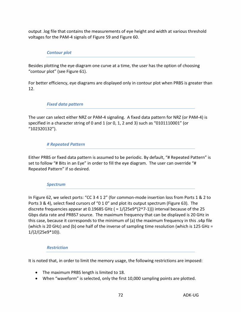
ADK-UG 72

output .log file that contains the measurements of eye height and width at various threshold voltages for the PAM-4 signals of Figure 59 and Figure 60.

Contour plot

Besides plotting the eye diagram one curve at a time, the user has the option of choosing “contour plot” (see Figure 61). For better efficiency, eye diagrams are displayed only in contour plot when PRBS is greater than 12.

Fixed data pattern

The user can select either NRZ or PAM-4 signaling. A fixed data pattern for NRZ (or PAM-4) is specified in a character string of 0 and 1 (or 0, 1, 2 and 3) such as “0101110001” (or “102320132”).

# Repeated Pattern

Either PRBS or fixed data pattern is assumed to be periodic. By default, “# Repeated Pattern” is set to follow “# Bits in an Eye” in order to fill the eye diagram. The user can override “# Repeated Pattern” if so desired.

Spectrum

In Figure 62, we select ports: “CC 3 4 1 2” (for common-mode insertion loss from Ports 1 & 2 to Ports 3 & 4), select fixed cursors of “0 1 0” and plot its output spectrum (Figure 63). The discrete frequencies appear at 0.19685 GHz ( = 1/(25e9*(2^7-1))) interval because of the 25 Gbps data rate and PRBS7 source. The maximum frequency that can be displayed is 20 GHz in this case, because it corresponds to the minimum of (a) the maximum frequency in this .s4p file (which is 20 GHz) and (b) one half of the inverse of sampling time resolution (which is 125 GHz = 1/(2/(25e9*10)).

Restriction

It is noted that, in order to limit the memory usage, the following restrictions are imposed:

• The maximum PRBS length is limited to 18. • When “waveform” is selected, only the first 10,000 sampling points are plotted.

ADK-UG 73

Figure 54

Figure 55

ADK-UG 74

Figure 56

----- Inputs ----- Input file = D:\Demo\Examples\ISD_SMA_to_SMA.s4p Selected ports = DD 3 4 1 2 Data rate = 25.78125 Gbps Rise time (20/80) = 10 ps Fall time (20/80) = 10 ps Amplitude (P-to-P) = 1 volt DC offset = 0 volt Random jitter = 0.01 UI Reference BER = 1e-05 Signaling = NRZ PRBS pattern = 7 TX Butterworth filter order = 2, bandwidth = 25 GHz RX Bessel filter order = 4, bandwidth = 25 GHz ----- Outputs ----- Optimized TX tap coefficients = -0.0651823 0.89267 -0.0421475 Optimized gDC for CTLE = -3 dB Optimized DFE coefficients = 0.00035264 0.00253746 -0.0127973 >>> Deterministic: *** Threshold voltage = 0 volt Eye height = 0.469299 volt Eye width = 34.682 ps Jitter = 4.10587 ps >>> With RJ=0.01 UI, BER=1e-05, Q=4.26489: *** Threshold voltage = 0 volt Eye height = 0.442286 volt Eye width = 31.191 ps Jitter = 7.59686 ps

Table 14

ADK-UG 75

Figure 57

Figure 58

ADK-UG 76

Figure 59

ADK-UG 77

Figure 60

----- Outputs ----- Optimized TX tap coefficients = -0.0570849 0.838403 -0.104512 >>> Deterministic: *** Threshold voltage = -0.2 volt Eye height = 0.158592 volt Eye width = 16.9354 ps Jitter = 23.0646 ps *** Threshold voltage = 0 volt Eye height = 0.157537 volt Eye width = 19.8503 ps Jitter = 20.1497 ps *** Threshold voltage = 0.2 volt Eye height = 0.156588 volt Eye width = 16.0715 ps Jitter = 23.9285 ps

Table 15

ADK-UG 78

Figure 61

ADK-UG 79

Figure 62

Figure 63

ADK-UG 80

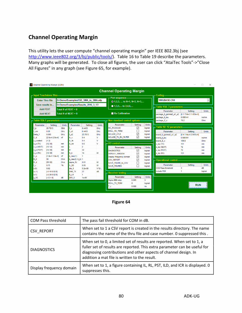
Channel Operating Margin This utility lets the user compute “channel operating margin” per IEEE 802.3bj (see http://www.ieee802.org/3/bj/public/tools/). Table 16 to Table 19 describe the parameters. Many graphs will be generated. To close all figures, the user can click “AtaiTec Tools”->”Close All Figures” in any graph (see Figure 65, for example).

Figure 64 COM Pass threshold The pass fail threshold for COM in dB.

CSV_REPORT When set to 1 a CSV report is created in the results directory. The name contains the name of the thru file and case number. 0 suppressed this .

DIAGNOSTICS

When set to 0, a limited set of results are reported. When set to 1, a fuller set of results are reported. This extra parameter can be useful for diagnosing contributions and other aspects of channel design. In addition a mat file is written to the result.

Display frequency domain When set to 1, a figure containing IL, RL, PST, ILD, and ICR is displayed. 0 suppresses this.

ADK-UG 81

DISPLAY_WINDOW When set to 0, the display window is suppressed. Set to 1 may be useful when running in a batch.

IDEAL_RX_TERM Normally set to 0. When set to 1, an ideal termination replaces the Tx package.

IDEAL_TX_TERM Normally set to 0. When set to 1, an ideal termination replaces the Rx package.

T_r Rise time of transmitter, converted to a TX filter per Equation 93A-46 if IDEAL_TX_TERM is true.

INC_PACKAGE

When set to 1, the package is added to the channel model. If the channel model contains a package set this to 0. When set to 0, C_d, z_p select, z_p (TX), z_p (NEXT),z_p (FEXT), z_p (RX), C_p, R_0, and R_d are ignored.

Include PCB This is normally set to 0. Set to 1 for CR4. When set to 1, a PCB board is concatenated on both sides of the tested channel as specified in 92.10.7.1.1.

INCLUDE_CTLE Normally set to 1. When set to 0, the CTLE is omitted from analysis.

INCLUDE_TX_RX_FILTER Normally set to 1. If set to 0, the Tx and Rx filter are omitted. However, Tx FFE and CTLE are not affected by this parameter.

Port Order order for s-parameter ports [ tx+, tx-, Rx+, Rx-]. Normally set to [1 3 2 4].

RESULT_DIR The name of the results directory. May use relative references.

RX_CALIBRATION Set to 0 for regular channel analysis. Set to 1 for calibrating the noise source in RX compliance test (Annex 93C.2).

Sigma BBN step Initial step used for noise adjustment in Rx calibration.

SAVE_FIGURE_to_CSV Set to one to save figure contents in .csv files in RESULTS_DIR.

SAVE_FIGURES Set to one to save .fig files in RESULTS_DIR.

Table 16

Table 93A-1 parameters

f_b Baud (Signaling) rate.

f_min Minimum start frequency for S parameters.

Delta_f Minimum frequency step size for S parameters.

C_d Device package model. Single-ended device capacitance (die pad).

z_p select z_p test cases to run, with corresponding z_p (TX), z_p (NEXT), z_p (FEXT), z_p (RX) values.

z_p (TX) List of victim transmitter package trace lengths in mm, one per case.

ADK-UG 82

z_p (NEXT) List of NEXT aggressor transmitter package trace lengths in mm, one per case.

z_p (FEXT) List of FEXT aggressor transmitter package trace lengths in mm, one per case .

z_p (RX) List of victim receiver package trace lengths in mm, one per case.

C_p Single-ended package-to-board capacitance (BGA ball).

R_0 Reference single-ended impedance.

R_d Device package model, Single-ended termination resistance

f_r Receiver 3 dB bandwidth for the 4th order Bessel-Thomson filter.

c(0) TX equalizer cursor minimum value (actual value is calculated as 1-c(-1)-c(1), skipped if smaller than the minimum).

c(-1) TX equalizer pre-cursor individual settings or range.

c(1) TX equalizer post-cursor individual settings or range.

g_DC Continuous time filter DC gain settings or range as specified in clause 93A.

f_z Continuous time filter zero frequency. Can be either a single value or a vector of the same length as g_DC.

f_p1 Continuous time filter first pole frequency. Can be either a single value or a vector of the same length as g_DC.

f_p2 Continuous time filter second pole frequency. Can be either a single value or a vector of the same length as g_DC.

A_v Victim differential peak output voltage (half of peak to peak).

A_fe Transmitter differential peak output voltage for Far-end aggressor.

A_ne Transmitter differential peak output voltage for Near-end aggressor.

L Number of symbols levels (PAM-4 is 4, NRZ is 2).

M Samples per UI.

N_b Decision feedback equalizer (DFE) length.

b_max(1) DFE magnitude limit, first coefficient (ignored if Nb=0).

b_max(2..N_b) DFE magnitude limit, second coefficient and on (ignored if Nb<2).

sigma_RJ Voltage sensitivity RMS Gaussian noise.

A_DD Normalized peak dual-Dirac noise, this is half of the total bound uncorrelated jitter (BUJ) in UI.

eta_0 One-sided noise spectral density.

SNR_TX Transmitter SNR noise (RMS).

R_LM Ratio of level separation mismatch. Relevant for PAM-4 only.

DER_0 Target detector error ratio.

Table 17

ADK-UG 83

Table 93A–3 parameters The package trace lengths in mm are specified with z_p (TX), z_p (NEXT), z_p (FEXT), and z_p (RX). The package loads are specified with C_d, C_p, R_0, and R_d.

package_tl_gamma0_a1_a2

Fitting parameters for package model per unit length. First element is in 1/mm that affects DC loss of package model. Second element is in ns1/2/mm that affects loss proportional to sqrt(f). Third element is in ns/mm that affects loss proportional to f.

package_tl_tau Represents propagation delay per unit length, for reflection effects.

package_Z_c Package model characteristic impedance.

Table 18

Table 92–12 parameters The board trace lengths in mm are specified with z_bp (TX), z_bp (NEXT), z_bp (FEXT), and z_bp (RX).

board_tl_gamma0_a1_a2

Fitting parameters for board trace model per unit length. First element is in 1/mm that affects DC loss of package model. Second element is in ns1/2/mm that affects loss proportional to sqrt(f). Third element is in ns/mm that affects loss proportional to f.

board_tl_tau Represents propagation delay per unit length, for reflection effects.

board_Z_c Board model characteristic impedance.

Table 19

ADK-UG 84

Figure 65

ADK-UG 85

IEEE and OIF Spec. With this utility, the user can choose among several IEEE and OIF specs, and compare the power sum of coupled noises, insertion loss crosstalk ratio (ICR), insertion loss, insertion loss deviation (ILD), and integrated crosstalk noise (ICN), etc. (See Figure 66 to Figure 70.) By default, the button: “Convert to Differential Signals” is enabled to convert single-ended S-param into differential S-param. Two types of port sequence are supported: (1) 1 to N as input and N+1 to 2N as output (which is preferred) and (2) 1, 3, …, 2N-1 as input and 2, 4, …, 2N as output. See Figure 21 for details about how the differential pairs are numbered.

Figure 66

ADK-UG 86

Figure 67 Power sum of far-end crosstalk (FEXT)

Figure 68 Insertion loss to crosstalk ratio (ICR)

ADK-UG 87

Figure 69 Insertion loss and fitted attenuation

Figure 70 Insertion loss deviation (ILD)

Figure 71 Return loss (RL)

ADK-UG 88

Extract 1X + 2X Traces Ideal for on-chip or small structure extraction, this utility allows the user to extract probe pad, trace and DUT models from multi-port measurement files. In general, the user inputs three Touchstone files for 1x thru, 2x thru and w/ DUT (see Figure 72 and Figure 73), and the program will output the models for pad, 1x trace and DUT (with the suffix of “pad1”, “trace1” and “DUT” attached to the file names). If the user inputs only two Touchstone files for 1x thru and 2x thru, then the program will output the models for pad and 1x trace only (with the suffix of “pad1” and “trace1” attached to the file names). If the user inputs only one Touchstone file for 1x thru, then the program will output a model (with the suffix of “pad0” attached to the file name) that is equal to the square root of 1x thru’s ABCD matrix. The user also has the option of choosing (1) the “port sequence”, (2) to de-embed from both sides, from the left side only or from the right side only and (3) to symmetrize 1x thru’s and 2x thru’s Touchstone files (e.g., to force S11=S22 in a 2-port file). Note that the DUT is assumed to be a through structure in this utility. To de-embed pad and trace from a non-through structure, the user can create pad and trace models using this utility first, followed by invoking the “De-embed [S]” utility with the selection of “Specified Ports”.

ADK-UG 89

Figure 72

ADK-UG 90

Figure 73

ADK-UG 91

Extract DK and DF With this utility, the user can extract DK, DF, roughness and 2D cross section from trace measurement data. Optionally, the user can create a new Touchstone file for any length and to any frequency. It is recommended that the user use In-Situ De-embedding (ISD) to remove the launch effect and obtain the trace-only data first. Either an .s2p or an .s4p file can be imported. This utility applies the wideband Debye (or Djordjevic-Sarkar) model for dielectric:

⋅+⋅+

⋅−

⋅∆+= ∞ fifi

mm m

m

1

2

1010log1

1012

εεε

and effective conductivity model (Gold & Helmreich, DesignCon 2014) for metal with surface roughness. Both magnitude and phase of insertion and return losses are simultaneously curvefitted. Figure 76 to Figure 77 show the extraction results for the example of Figure 74 where the original 2" trace-only data, up to 40GHz, are curvefitted and a model is created to generate a new Touchstone file (in …_fit.snp) for 2" trace to 50 GHz. This example Touchstone file can be found in the .zip file you download from the web. The output graphs (Figure 75) show the trace impedance and effective conductivity. In Figure 77, eri = ∞ε and erd = ε∆ for the Debye equation above. For good curvefitting:

• "Auto de-skew" can be enabled to de-skew a differential pair for unbiased reading of insertion loss. When "Auto de-skew" is enabled, a new file (in …_noskew.s4p) will be created and used for later processing. The amount of deskew is displayed in the command window. "Auto de-skew" is ignored if the input file is in .s2p.

• Accurate length and stackup (td1, td2, tm) are most important and should be entered accordingly.

• The program numerically optimizes width (wt, wb), pitch, DK, DF and rms roughness (Rq) to match both magnitude and phase of insertion and return losses. Good initial guess of wt, wb, pitch, DK, DF and roughness will help, though not absolutely necessary. After finishing each run, the program automatically updates the above variables in the GUI window. Clicking "Run" again with the updated variables may refine the results further.

Stripline vs. Microstrip

Two templates are supported: stripline with homogeneous dielectric and microstrip with conformal solder mask. In the microstrip case (Figure 78), the solder mask is assumed to have

ADK-UG 92

constant dielectric (DK2) with zero loss tangent. DK2 will not be numerically optimized so an accurate number of DK2 should be entered when the microstrip template is selected.

Delta L

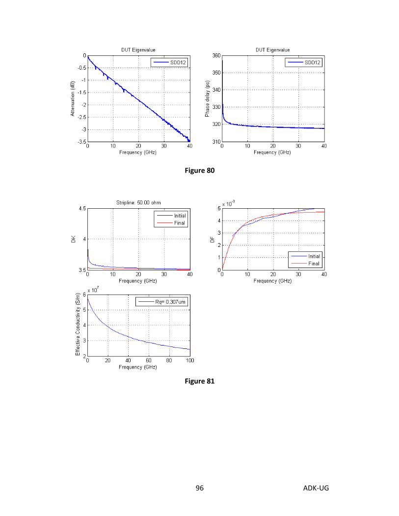
Instead of entering a Touchstone file for de-embedded trace-only data, the user has the option of entering two Touchstone files: one for short trace + launch and another for long trace + launch. The program will then estimate the trace-only attenuation through eigenvalue (or Delta-L) solution and create a new file in …_deltaL.snp. (For details about eigenvalue solution, see Page 14 of http://www.ataitec.com/PDF/Paper_AfullyautomatedSIPlatform.pdf ) Because no return loss information is available, the trace impedance is assumed to be the same as reference impedance in the Touchstone files, resulting in different extracted values (Figure 79 to Figure 82). When "Auto de-skew" and "Create new Touchstone file" are enabled with "Delta L", the following files will be created for .s4p input files: <short trace file name>_noskew.s4p

<long trace file name>_noskew.s4p <long trace file name>_noskew.s4p_deltaL.s4p <long trace file name>_noskew.s4p_deltaL.s4p_fit.s4p

and, for .s2p input files:

<long trace file name>_ deltaL.s2p <long trace file name> _deltaL.s2p_fit.s2p

ADK-UG 93

Figure 74

Figure 75

ADK-UG 94

Figure 76

Input file = D:\mpx_for_ISD\MPX_L7_T5_WS1_Z90_T1234.s4p_DUT.s4p_noskew.s4p --- Stripline --- Optimized eri=3.48419, erd=0.0483458, m1=9.82888, m2=11.4027 sigma=5.8e+07 S/m, roughness=0.320932 um wt=5.40648 mil, wb=5.40648 mil, pitch=14.3688 mil Fixed td1=5.6 mil, td2=6.1 mil, tm=1.2 mil Constant DK=3.51306, DF=0.0043646 Ref Z=44.6618 ohm GHz Effective Conductivity (S/m) DK DF 0.1 5.751924e+07 3.532539 0.000055 0.2 5.727834e+07 3.532535 0.000109

Figure 77

ADK-UG 95

Figure 78

Figure 79

ADK-UG 96

Figure 80

Figure 81

ADK-UG 97

Figure 82

ADK-UG 98

x2D: 2D Field Solver x2D is a 2D RLGC field solver, which accepts inputs either directly from the graphical user interface (GUI) or from a user-defined file. Through GUI (Figure 83 to Figure 84), the user can enter the thickness, top/bottom width, and spacing in scalar or vector form to specify the cross section of each conductor in multi-layered structures. When the number of thickness, top/bottom width, or spacing is less than the specified number of conductors in each layer, the last entered thickness, top/bottom width, or spacing is assumed for the rest of conductors. When the number of thickness, top/bottom width, or spacing is greater than the specified number of conductors in each layer, those entries past the number of conductors are ignored. The user can also ground or float conductors by entering their indices. The sequence of conductor number starts from 1 at the leftmost conductor on the bottom layer and increases from left to right and lower to higher layer. An example of user-defined file is shown in Figure 86, where Er=dielectric constant, tanD=loss tangent, and the division flag=1 (for cosine-weighted mesh), 2 (for cosine-weighted left-shoulder mesh), 3 (for cosine-weighted right-shoulder mesh), or 4 (for uniform mesh). Each segment is associated with one Er and tanD on the right side of segment and another Er and tanD on the left side of segment. The direction of each segment is defined by "from-node" to "to-node". The same Er and tanD are specified for both left and right sides of a conductor segment. This sample file corresponds to the GUI data of Figure 84, and is generated automatically when the GUI data are run. Additional templates, shown in Figure 87 to Figure 93, are available to simplify the simulation of connectors and cables.

Figure 83

ADK-UG 99

Figure 84

Figure 85

ADK-UG 100

68 -> no. of nodes 7 -> no. of conductors (except ground) 4 -> no. of segments for 1st conductor 4 -> no. of segments for 2nd conductor 4 -> no. of segments for 3rd conductor 4 -> no. of segments for 4th conductor 4 -> no. of segments for 5th conductor 4 -> no. of segments for 6th conductor 4 -> no. of segments for 7th conductor 30 -> no. of ground conductor segments 8 -> no. of dielectric segments -5 0.26 -> x, y coordinates of 1st node 16.34 0.26 -> x, y coordinates of 2nd node 0 0.26 -> : -0.14 0.5 6 -> : 0.42 0.26 0.56 0.56 3.42 0.26 3.48 0.41 3.84 0.26 3.78 0.41 4.92 0.26 4.98 0.41 5.34 0.26 5.28 0.41 6.42 0.26 6.28 0.56 6.84 0.26 6.98 0.56 7.92 0.26 7.98 0.41 8.34 0.26 8.28 0.41 9.42 0.26 9.48 0.41 9.84 0.26 9.78 0.41 10.92 0.26 10.78 0.56 11.34 0.26 11.48 0.56 0 0 0.42 0 -5 0 3.42 0 3.84 0 0.42 0 4.92 0 5.34 0 3.84 0 6.42 0 6.84 0 5.34 0 7.92 0 8.34 0

ADK-UG 101

6.84 0 9.42 0 9.84 0 8.34 0 10.92 0 11.34 0 9.84 0 16.34 0 0 1.86 0.42 1.86 -5 1.86 3.42 1.86 3.84 1.86 4.92 1.86 5.34 1.86 6.42 1.86 6.84 1.86 7.92 1.86 8.34 1.86 9.42 1.86 9.84 1.86 10.92 1.86 11.34 1.86 16.34 1.86 3 5 3.6 0.01 3.6 0.01 3 1 -> from-node id, to-node id, Er (right), tanD (right), Er (left), tanD (left), no. of meshes, division flag for 1st segment 4 6 1 0 1 0 3 1 -> from-node id, to-node id, Er (right), tanD (right), Er (left), tanD (left), no. of meshes, division flag for 2nd segment 3 4 1 0 1 0 3 1 5 6 1 0 1 0 3 1 7 9 3.6 0.01 3.6 0.01 3 1 8 10 1 0 1 0 3 1 7 8 1 0 1 0 3 1 9 10 1 0 1 0 3 1 11 13 3.6 0.01 3.6 0.01 3 1 12 14 1 0 1 0 3 1 11 12 1 0 1 0 3 1 13 14 1 0 1 0 3 1 15 17 3.6 0.01 3.6 0.01 3 1 16 18 1 0 1 0 3 1 15 16 1 0 1 0 3 1 17 18 1 0 1 0 3 1 19 21 3.6 0.01 3.6 0.01 3 1 20 22 1 0 1 0 3 1 19 20 1 0 1 0 3 1 21 22 1 0 1 0 3 1 23 25 3.6 0.01 3.6 0.01 3 1 24 26 1 0 1 0 3 1 23 24 1 0 1 0 3 1 25 26 1 0 1 0 3 1 27 29 3.6 0.01 3.6 0.01 3 1 28 30 1 0 1 0 3 1 27 28 1 0 1 0 3 1 29 30 1 0 1 0 3 1 33 31 3.6 0.01 3.6 0.01 8 2

ADK-UG 102

31 32 3.6 0.01 3.6 0.01 3 1 36 34 3.6 0.01 3.6 0.01 5 1 34 35 3.6 0.01 3.6 0.01 3 1 39 37 3.6 0.01 3.6 0.01 3 1 37 38 3.6 0.01 3.6 0.01 3 1 42 40 3.6 0.01 3.6 0.01 3 1 40 41 3.6 0.01 3.6 0.01 3 1 45 43 3.6 0.01 3.6 0.01 3 1 43 44 3.6 0.01 3.6 0.01 3 1 48 46 3.6 0.01 3.6 0.01 3 1 46 47 3.6 0.01 3.6 0.01 3 1 51 49 3.6 0.01 3.6 0.01 3 1 49 50 3.6 0.01 3.6 0.01 3 1 50 52 3.6 0.01 3.6 0.01 8 3 55 53 1 0 1 0 8 2 53 54 1 0 1 0 3 1 54 56 1 0 1 0 5 1 56 57 1 0 1 0 3 1 57 58 1 0 1 0 3 1 58 59 1 0 1 0 3 1 59 60 1 0 1 0 3 1 60 61 1 0 1 0 3 1 61 62 1 0 1 0 3 1 62 63 1 0 1 0 3 1 63 64 1 0 1 0 3 1 64 65 1 0 1 0 3 1 65 66 1 0 1 0 3 1 66 67 1 0 1 0 3 1 67 68 1 0 1 0 8 3 1 3 3.6 0.01 1 0 8 2 5 7 3.6 0.01 1 0 5 1 9 11 3.6 0.01 1 0 3 1 13 15 3.6 0.01 1 0 3 1 17 19 3.6 0.01 1 0 3 1 21 23 3.6 0.01 1 0 3 1 29 2 3.6 0.01 1 0 8 3 25 27 3.6 0.01 1 0 3 1 1e-3 -> unit (mm: 1e-3, mil: 25.4e-6, um: 1e-6, in: 2.54e-2) 5e7 -> conductivity in S/m 3 -> frequency in GHz 1 4 7 -> indices of additional grounding conductors (0 for none) 0 -> indices of additional floating conductors (0 for none) 1 -> order of differential pair (1 for 1->2, 3->4, …, and 2 for 1-> n/2+1, 2->n/2+2, …)

Figure 86

ADK-UG 103

Figure 87

Figure 88

Figure 89

ADK-UG 104

Figure 90

Figure 91

ADK-UG 105

Figure 92

Figure 93

ADK-UG 106

Batch The user can also easily process multiple ADK utilities by clicking “Batch” and running ADK in a batch mode. A batch-mode window (Figure 94) prompts the user for an input text file with .abt extension and syntax shown in Figure 95.

System command To automate ADK runs in a program, the user can launch batch-mode ADK by the following system command, for example:

“C:\Program Files (x86)\AtaiTec\ADK\adk2.exe” adkc D:\input.abt where “C:\Program Files (x86)\AtaiTec\ADK\adk2.exe” is the full-path executable name surrounded by two double quotes (") and D:\input.abt is a full-path input file name.

Figure 94

ADK-UG 107

Batch file Explanation

! Sample ADK batch file # connection infile E:\Demo\test.s4p quality 0 # passive infile E:\Demo\test.s4p reciprocal 1 passive 1 causal 0 zero_t 1 mix_mode_method 1 plot 0

! in the first letter indicates a comment. # connection is a keyword to invoke "Find connection". Keywords and variables are case-insensitive. The variable name infile is followed by an input Touchstone file. 0 (default) to check connection only; 1 to also check infile's passivity and causality; 2 to check connection, passivity and causality of entire directory. # passive invokes “Passivity & Causality”. Input file. 1 (default) to enforce reciprocity of [S] matrix and 0 to disable 1 (default) to enforce passivity of [S] matrix and 0 to disable 0 (default) to disable and 1 to correct causality. 1 (default) to zero out waveform at T<0 before applying Krameres-Kronig criteria for causality correction; 2 to apply Kramers-Kronig only; 3 to zero out waveform at T<0 only. 1 (default) to apply causality correction to mixed-mode [S]; 0 to apply causality correction to single-ended [S]. Used only causal is set to 1. 0 (default) to turn off

ADK-UG 108

dc_method 1 resistance 0.05 ground 0 connection 0 reverse 1 2 # s2mix infile E:\Demo\test.s4p_pass.s4p mixed 1 order 0 # s2tdr infile E:\Demo\test.s4p

figures and 1 to turn on. Method to correct DC: 1 (default) to use DC resistance, 2 to extrapolate and 3 to use original value in the Touchstone file. Signal’s DC resistance (in ohm) for DC method 1; default is 0.05. Multiple numbers (such as “resistance 0.5 0.3 0.1”) can be used for different resistance in each signal. Ground return’s DC resistance (in ohm) For DC method 1; default is 0. Order of port connection: 0 (default) for the program to find out; 1 for (1,2,3) in and (n+1, n+2, n+3) out; 2 for (1,3,5) in and (2,4,6) out; and 3 for no through connection. Reverse polarity of specified ports (optional) # s2mix invokes “Single to Mixed Mode” conversion Input file. A wildcard character "*" can be used in the file name (not directory name) to process multiple files. 1 (default) for differential only, 2 for common only, 3 for mixed mode Differential pair order: 0 for default, 1 for (1,2), (3,4), …, and 2 for (1, N/2+1), (2, N/2+2) pair. # s2tdr invokes S to “TDR & TDT” conversion Input file

ADK-UG 109

differential 0 ports dd 1 2 step_response 1 tdr_out 1 rise_time 41.4448e-12 bit_time 100e-12 duration 5e-9 resolution 5e-12 delay 1e-9 amplitude 2 bandwidth 6.3337e9 rolloff -20 filter 1 # scale

0 (default) for single-ended, 1 for differential-mode and 2 for common-mode signals Port indices (optional) to plot individual curve. 1 (default) for step response, 2 for single-bit response, and 0 for impulse response 1 for impedance profile, 2 for TDR with open termination, and 3 for TDR & TDT with matched termination; default is 1 for impedance profile. Input rise time (20% to 80%) before filter; default is 41.4448 ps. Bit time for single-bit response (default is 100 ps) Duration of waveform (default is 5 ns) Resolution of waveform (default is 5 ps) Delay of waveform. Default is 0 ns. Amplitude of input waveform (default is 2 volt) Bandwidth of filter. Default is calculated by 0.35/((rise_time/0.6)*0.8), if not specified. Filter has -20 dB/dec (default) roll-off beyond bandwidth 1 (default) for Butterworth filter and 0 for Brickwall filter # scale invokes “Change Impedance” to scale impedance and length, and change reference impedance

ADK-UG 110

infile E:\Demo\test.s4p zref 42.5 zscale 1.05 lscale 1 format 2 csvflag 0 syzflag 1 # s2spice infile E:\Demo\test.s4p npoles 40 reciprocal 1 passive 1 matchdc 1 samepoles 0 npoints 201 minfreq 0 maxfreq 20e9

Input file Change output reference impedance (default is 50 ohm) Scale impedance (default is 1) Scale length (default is 1) Output Touchstone file format in MA (1), DB (2) or RI (3). Default is 2. Save additional .csv file. Yes=1 and no=0 (default). Output Touchstone file in S (1), Y (2) or Z (3). Default is 1. # s2spice invokes the utility to convert S to SPICE models Input file Number of poles (40 is default) 1 (default) to enforce reciprocity of [S] matrix and 0 to disable 1 (default) to enforce passivity of [S] matrix and 0 to disable 1 (default) to match DC values and 0 to disable 1 to use same poles for entire [S] and 0 (default) to disable Number of points for new Touchstone file; default is 0 to turn off creation of new Touchstone file. Minimum frequency for new Touchstone file (default is 0) Maximum frequency for new Touchstone file (default is 20 GHz)

ADK-UG 111

linear 1 plot 0 # spice2s infile E:\Demo\test.cir minfreq 0 maxfreq 20e9 npoints 201 linear 1 zref 50 plot 0 # cascade infile E:\Demo\test.s4p infile E:\Demo\test.s4p outfile E:\Demo\test.s4p_casc.s4p Zref 50 Order 1 zleft 50

Flag for frequency spacing (1=linear and 2=log). Default is 1 (linear). 0 (default) to turn off figures or 1 to turn on. # spice2s invokes the utility to convert SPICE models to S Input file name. The output file name is in …_new.sXp Minimum frequency for new Touchstone file (default is 0) Maximum frequency for new Touchstone file (default is 20 GHz) Number of points for new Touchstone file; default is 201. Flag for frequency spacing (1=linear and 2=log). Default is 1 (linear). Reference impedance. Default is 50 ohm. 0 (default) to turn off figures or 1 to turn on. # cascade invokes the utility to cascade multiple [S] Input file name. Multiple input files can be entered. Output file name. If not specified, the default is to append _casc.sXp to the first input file name. Output reference impedance. Default is 50 ohm. Port sequence. 1 (default) for 1->N+1, 2->N+2, …, N->2*N and 2 for 1->2, 3->4, …. Impedance (default is 50 ohm)

ADK-UG 112

tleft 10e-12 zright 50 tright 20e-12 # interpolate infile E:\Demo\test.s4p minfreq 0 maxfreq 20e9 npoints 201 linear 1 mixed 1 passive 1 bad_frequency 1.7e9 smooth_transition 1e9 plot 0 # combine

for optional transmission line padding from the left. Delay (default is 0) for optional transmission line padding from the left. Impedance (default is 50 ohm) for optional transmission line padding from the right. Delay (default is 0) for optional transmission line padding from the right. # interpolate invokes the utility to interpolate [S] Input file name. The output file name is in …_new.sXp Minimum frequency for new Touchstone file (default is 0) Maximum frequency for new Touchstone file (default is 20 GHz) Number of points for new Touchstone file (default is 201) Flag for frequency spacing (1=linear and 2=log). Default is 1 (linear). Use mixed-mode method (0=off and 1=on). Default is 0. Turn on (1=default) or off (0) passivity and reciprocity correction. Remove bad frequency points (optional). Smooth transition frequency range for extrapolation (optional). 0 (default) to turn off figures or 1 to turn on. # combine invokes the utility

ADK-UG 113

infile E:\Demo\test.s4p 1 2 3 4 infile E:\Demo\test.s4p 5 6 7 8 outfile E:\Demo\test_out.s8p method 1 nports 8 # extract infile E:\Demo\test_out.s8p outfile E:\Demo\test_new.s4p new_port_sequence 5 6 7 8 extract_all_s4p 0 # create pecfile E:\Demo\test_pec.s2p pmcfile E:\Demo\test_pmc.s2p outfile E:\Demo\test_create.s4p

to combine and expand multiple Touchstone files Input file followed by new port indices; Multiple input files can be entered. Output file. If not specified, the default is to append _combine.sXp to the first input file name. 1 (default) to combine by S or 0 to combine by Z. Total number of ports after expansion. The default is to use the maximum port index found under “infile”. # extract invokes the “Extract or Re-order” utility to extract a smaller Touchstone file or to reorder the port numbers Input file Output file Port numbers from Input file that will be extracted or re-ordered 0=off (default), 1 to extract all .s4p files with (1,2), (3,4), … pairs and 2 to extract all .s4p files with (1,3), (5,7), … pairs. If set to 1 or 2, outfile and new_port_sequence are ignored. # create invokes the utility to combine Touchstone files with PEC and PMC conditions and create a new Touchstone file Input file with PEC condition Input file with PMC condition Output file name. If not specified, the default is to

ADK-UG 114

port_on_axis 2 new_port_sequence 1 2 3 # mplot infile E:\Demo\test.s4p dd 1 2 infile E:\Demo\test.s4p 1 3 outfile E:\Demo\test.bmp outfile E:\Demo\test2.bmp display 1 syzflag 1 zref 42.5 spec 0 -10 20 -10 size 4 3 xrange 5 15 yrange -20 0 xlabel frequency (GHz) ylabel Insertion Loss (dB) linewidth 2

append _create.sXp to PEC file name. Port indices that crosses the symmetry axis. (Optional) New port sequence. (Optional) # mplot invokes the utility to plot multiple curves and save to a .bmp file Input file followed by single-ended or mixed-mode port indices; Multiple input files can be entered. Output .bmp file. Other extensions (.jpg, .tif, .pdf and .fig) can be used to save into other formats. 2nd output .bmp file for phase. Optional. 1 (default) to display graphs on screen. 0 to close. 1 (default) to plot S or TDR/TDT; 2 to plot Z, 3 to plot Y, 4 to plot VSWR, 5 to plot L and 6 to plot Smith chart. Re-normalize impedance (Optional) Spec curve in “x1 y1 x2 y2 …” (Optional) Size in inches for x and y dimensions. (Optional) Range (in GHz or ns) for x axis. (Optional) Range (in dB, ohm or volt) for y axis. (Optional) Label for x axis. (Optional) Label for y axis. (Optional) Line width (1 to 5) for all curves. Default is 1.

ADK-UG 115

linecolor brkmcg logplot 0 phase_delay 0 length 1.5 2 1.2 title Plotting Example legend SDD12 legend S13 math 20*(log10(abs(s2))-log10(abs(s1))) savecsv 0 # standard infile E:\Demo\test.s28p spec_no 1 differential 1 baud_rate 10.3125e9

Line color for curves in sequence. Default is brkmcg (b: blue, r: red, k: black, m: magenta, c: cyan, g: green) Flag for linear (0) or log (1) plot. Default is 0. Flag (0 or 1) to plot phase delay. (Default is 0 to plot phase angle instead of phase delay.) Length (in inches), if specified with "phase_delay 1", plots DK values. A vector of numbers can be entered to specify length for each curve. Figure title. (Optional) Legend for each curve. Multiple legends can be specified. (Optional) Math expression (optional) to add another curve. Flag (0 or 1) to save graph in .csv file. Default (0) is to not save. # standard invokes the utility to compare with various IEEE and OIF specs. Input file name. Spec (1: 10Gbase-KR, 2: 40GBase-CR4, 3: CEI-25G-LR, 4: CEI-28G-MR or 5: CEI-28G-VSR). Default is 1. Flag (0 or 1) to turn off or on differential conversion. Default is 1. Baud rate (in bps). Default is 10.3125e9, 10.3125e9, 25.8e9, 28.05e9 and 28.1e9 for spec_no=1 to 5, respectively.

ADK-UG 116

ref_freq 5e9 log_plot 0 fit_icr 0 minfreq 0.1e9 maxfreq 5.15625e9 il 1 7 rl 1 1 xtalk 1 2 xtalk 1 3 xtalk 1 4 size 8 6 figure_tag testRun csv_tag test # eye

Reference frequency (in Hz) beyond which a constant ICR spec is used for 10GBase-KR. Flag (0 or 1) to turn off or on the log(f) plot. Default is 0. Flag (0 or 1) to turn off or on ICR curve fitting. Default is 0. Min. frequency (in Hz) for ICR curve fitting. Default is 0.1e9 Hz. Max. frequency (in Hz) for ICR curve fitting. Default is 5.15625e9 Hz. Insertion loss index. Return loss index. Xtalk index. Multiple xtalk (up to 50) can be specified. Figure size in inches in x and y dimension. Default is 8 for x and 6 for y. By default, all figures are saved in .bmp with 10gKR, 40gCR4, 25gLR, 28gMR and 28gVSR appended to the input file name. The appended string can be overridden by the text (“testRun” in this case) specified after the keyword “figure_tag”. When csv_tag (optional) is present, all figures will also be saved in .csv files (under the name of xxx.test.rl.csv, xxx.test.ild.csv, etc. in this case). The default is to NOT output the .csv files. # eye invokes the utility to simulate eye diagrams (through “Channel Optimization”)

ADK-UG 117

infile D:\Demo\example4_s2spice.s8p outfile D:\Demo\test.bmp ports dd 5 6 1 2 ports dd 5 6 3 4 baud_rate 5e9 rise_time 50e-12 pam4 1 prbs 7 rj 0 ber 1e-5 nsamples 20 contour_plot 0 ffe 0 nprecursor 1 npostcursor 1 min_maincursor 0.5 cursor 0 1 0 ctle 0 gdc -10 1 0

Input file name. Save output graphics (optional). Formats in .bmp, .jpg, .tif, .pdf and .fig can be used. Selected ports; default is “dd 3 4 1 2”. Multiple ports can be specified to add crosstalks. Baud rate (in bps); default is 5e9. Rise time (20% to 80%) in seconds; default is 50e-12. 0 (default) for NRZ and 1 for PAM4. PRBS data pattern; default is 7. Random jitter. Default is 0. Must be between 0 and 0.1. Reference BER. Must be between 1e-40 and 0.1 Default is 1e-5. Number of samples per bit; default is 20. Contour plot. 0 (default) to turn off or 1 to turn on. TX FFE. 0 (default) to turn off or 1 to turn on. Number of TXFFE precursors. Default is 1. Number of TXFFE postcursors. Default is 1. Minimum main cursor for TXFFE. Default is 0.5. Fixed cursors. Default is “0 1 0”. Used only when ffe is set to 0. RX CTLE. 0 (default) to turn off or 1 to turn on. gDC sweep when ctle is set to

ADK-UG 118

ndfe 0 butter_filter 0 butter_order 2 butter_bandwidth 25e9 bessel_filter 0 bessel_order 4 bessel_bandwidth 25e9 neyes 2 delay 103.16e-12 minvolt -0.6 maxvolt 0.6 threshold -0.35 0 0.35 eyemask 50 0 100 -0.1 150 0 100 0.1 50 0 eyemask 50 0.32 100 0.22 150 0.32 100 0.42 50 0.32 eyemask 50 -0.32 100 -0.22 150 -0.32 100 -0.42 50 -0.32

1. Default is “-10 1 0” for sweeping from -10 to 0 dB at 1 dB increment. Number of DFE taps. Default is 0. Butterworth filter for TX. 0 (default) to turn off or 1 to turn on. Order of TX Butterworth filter. Default is 2. Bandwidth of TX Butterworth filter. Default is 25e9 in Hz. Bessel filter for RX. 0 (default) to turn off or 1 to turn on. Order of RX Bessel filter. Default is 4. Bandwidth of RX Bessel filter. Default is 25e9 in Hz. Number of bits in an eye. Default is 2. Delay (in seconds) to shift eye diagram. Default is 0. Minimum voltage (in volt) for eye diagram. Default is -0.6. Maximum voltage (in volt) for eye diagram. Default is 0.6. Threshold voltage(s) in volt to compute eye height and eye width. Default is 0. Optional eye mask in “x1 y1 x2 y2 x3 y3…” format. Multiple eyemask’s can be specified.

ADK-UG 119

savecsv 0 # print infile E:\Demo\test.s4p_scale.s4p freq 3.125e9 6.25e9 12.5e9 # system copy E:\Demo\adkbatch.abt E:\test.abt rename E:\test.abt temp.abt del E:\temp.abt

Flag (0 or 1) to save graph in .csv file. Default (0) is to not save. # print invokes the utility to print [S] at specific frequencies. Input file Print S at 3.125, 6.25 and 12.5 GHz # system is a keyword to run such system commands as rename, copy, del, move, …; Enter “help” under Command Prompt in Windows to see all available commands.

Figure 95

ADK-UG 120

Appendix

ADK and ISD Installation (for all Windows) 1. Download and install “Matlab Compiler Runtime 8.0” by running

http://ataitec.com/download/MCR_R2012b_win32_installer.exe

or

http://ataitec.com/download/MCR_R2012b_win32_installer.exe

Make sure that the file size is 351,078 KB. You will get MCR error later if the download file is incomplete.

(You can skip this step if you have installed the Matlab Compiler Runtime 8.0 before.)

2. Download and extract the ADK and ISD .zip file from

http://ataitec.com/download/ADK_ISD.zip

The user guides and examples are in the .zip file. Install ADK and ISD by executing

AtaiTec_SI_Suites_xxxx.xx.msi 3. Install ADK (and ISD) licenses:

Click “All Programs->Accessories->Command Prompt”; Enter “ipconfig /all”; Copy down Physical Address and send it to AtaiTec; Obtain XXX.lic (a license file in .lic extension) from AtaiTec. If you have a floating license, change the hostname in XXX.lic from “localhost” to the server’s hostname. (If you have a node-locked license, there is no hostname to change.) By default, the port number is set to 5053. Change this port number if necessary. For more details, please see: http://www.reprisesoftware.com/RLM_Enduser.html Save XXX.lic under the directory where ADK and ISD were installed (such as C:\Program Files \AtaiTec\License or C:\Program Files (x86) \AtaiTec\License).

4. Run ADK (or ISD)

ADK-UG 121

If you have a node-locked ADK (or ISD) license, simply double-click the ADK (or ISD) icon to run. If you encounter MCR error, check the following: • Was the Matlab Compiler Runtime downloaded completely and installed correctly?

• Enter “path” under Command Prompt. Add the following path to Matlab Compiler

Runtime if it does not appear:

C:\Program Files (x86)\MATLAB\MATLAB Compiler Runtime\v80\runtime\win32

• Reboot the computer. If you have a floating license, make sure you complete Steps 1 to 3 on BOTH server and client computers first. Click “All Programs->AtaiTec SI Suites->License Server” in the server computer. Then, double-click the ADK (or ISD) icon in the client computer to run. Note: (a) The server’s and client’s Command windows contain the license and program status. (b) Closing either server’s or client’s Command window will result in the termination of running ADK or ISD. (c) You don’t need to click “All Programs->AtaiTec SI Suites->License Server” in the client computer. Figure 96 shows an example of floating license where “localhost” is to be renamed to the server’s hostname, “5053” is the default port number which can also be modified, “2012.06” is the maintenance expiration date (or the highest ADK version number for which this license will run), “31-dec-2012” is the license expiration date, and the number “1” before “issued” indicates the number of licenses available.

HOST localhost 0013e86eceed 5053 ISV ataitec LICENSE ataitec adk2 2012.06 31-dec-2012 1 issued=30-jun-2011 _ck=40d6d2f02a sig="c2S25g2K4gm29XCXm+EstFkqEFi+pQ8+BN8mqvbHg581x*0 M4kNg3Ay5YUBfJV8" LICENSE ataitec isd2 2012.06 permanent 1 issued=30-jun-2011 _ck=6b36cac159 sig="c2W25g2x67Asneus~KVnno5Wrk~bQ9joQg8n0aJ0PghedTs JW6PU=xmHKZoPNwsq"

Figure 96

5. To install an updated ADK and ISD release (if you have previously installed ADK and ISD):

ADK-UG 122

Remove the existing ADK and ISD through Control Panel->Add or Remove Programs->AtaiTec SI Suites->Remove, then go to Step 2. (You do not need to remove the “Matlab Compiler Runtime Library”.)

ADK-UG 123

ADK and ISD Server for Linux on Intel 64bit The ADK and ISD executables do not run on Linux. However, if you have a floating license, you can start the license server from an Intel 64bit computer with Linux OS, check out the license from that server, and run ADK or ISD from Windows-based computers. To install the license server on an Intel 64bit computer with Linux OS (not Solaris or HPUX): 1. Download the ADK and ISD license server from

http://ataitec.com/download/AtaiTec_on_Linux.tar

Extract the downloaded .tar file by entering tar –xvf AtaiTec_on_Linux.tar There are several files in the directory: ataitec.set rlm rlmutil testlic

2. Save the license file XXX.lic in the same directory. (Modify XXX.lic for the correct hostname and port number if necessary. Please see the previous pages and http://www.reprisesoftware.com/RLM_Enduser.html for more details.)

3. Start the license server (and keep it running) by entering rlm & You can test the license by entering testlic 4. Follow the steps in “ADK and ISD Installation” to install ADK and ISD on Windows-based

computers, copy the license file XXX.lic to the license directory (…/License), and click ADK or ISD icon to run.