A38 Monitoring manual for bitou bush control and native plant recovery

Additional information The following section provides additional details on the sampling methods described above, for users who wish to learn more about monitoring and generating high quality data. Additional information is included on:

sampling methods measuring vegetation, including

o indices of abundance o demographic measures o response to control

understanding experimental design, and considerations when selecting sampling units.

Sampling methods The following section outlines some additional notes on the three sampling methods used in this manual. They are designed to help you better understand the prescribed methods.

Line-intercept transects Three measures of abundance can be made using the line-intercept method: density, cover, and presence/absence. However, the density technique produces a measure that is ambiguous and dependent on the size of the species being measured, and so is not recommended. The description in this manual therefore only refers to cover (and to a lesser degree presence/absence – floristic survey).

From a species perspective, the line-intercept technique lends itself readily to measuring the cover of shrubs and matted plants; it is less effective for plants with lacy or narrow canopies such as grasses and some forbs. Line-intercept transects can be used quickly for plants with low but densely clustered cover, and they are more practical in sparse vegetation than quadrats. Plants that are sparse, small and well-distributed along a line will require more meticulous evaluation of the transect.

Line-intercept transects are commonly used for shrubs that are less than 1.5 m tall because a tape can be suspended above the shrub canopy and the interception easily measured. Irrespective of the height of the transect, however, you should abide by the definition of cover as the vertical projection on the ground.

Quadrats Biases in quadrat sampling relate to the census technique used. For cover and density, more conspicuous species are likely to be observed and those forming clumps of individuals with broader leaves are likely to be given a higher estimate than those that are less conspicuous, dispersed or with fine-leaves. Careful sampling should overcome this bias.

Very large quadrats can be difficult and time consuming to set up and measure on a regular basis. If species have a non-random distribution over the study area (a common occurrence for plants) then estimates of abundance from a single quadrat will be heavily influenced by the size of the quadrat. Larger quadrats will capture more of the patchiness in the vegetation than smaller quadrats. For this reason single quadrats should never be used. Selecting the appropriate quadrat size, number and spacing according to the vegetation type should help eliminate these effects.

T-square sampling The core area in which T-square sampling occurs should be slightly smaller than the total monitoring area, to allow for the possibility that the nearest individuals to some of the random starting points might be outside the core area. Ideally, the number of random starting points should be greater than 10 (Sutherland 2006).

Advanced monitoring techniques – additional information A39

T-square sampling does not suffer the same degree of bias when individuals are distributed non-randomly as several other nearest-neighbour measures, however it is still advisable to apply a test of randomness to the data. A simple test for randomness is:

ti = {∑i [xi2 / (xi

2 + yi2 / 2)] – m/2}√(12/m)

where: xi = the distance from the random starting point to the nearest tree

yi2 = the distance from the nearest tree (xi) to its nearest neighbour

m = the number of random starting points

If ti is greater than +2 then the distribution is significantly more regular than a random distribution (i.e. dispersed); if it is less than –2 then it is significantly clumped; if it is between -2 and +2 it is considered random. This is an approximate test only; refer to Diggle (1983) for further details.

Measuring vegetation Indices of abundance Cover

Cover (also called canopy cover) is the vertical projection of vegetation from the ground as viewed from above. Cover is a commonly used measure as it enables all species to be compared irrespective of their size or abundance (e.g. from small but abundant to large but rare). Unlike density (see below), cover is closely aligned with biomass or annual production. Cover does not require the ability to distinguish between individuals of the same species. It is, however, sensitive to changes over the growing season. Although the lack of native deciduous species makes this less of an issue in Australia than elsewhere in the world, sampling should be repeated at the same stage of the growing season.

There are a number of ways to estimate cover. When using quadrats, an observer estimates the proportion of the quadrat occupied by a species. In addition to estimating the actual percentage of the quadrat covered by a species, the observer can categorise cover estimates, for example into cover classes, percentage cover ranges, or cover categories (see page 32 of the Standard tier; also Table A8 below). While estimating cover in quadrats is fast in comparison to counting each individual of a species, the estimate is subjective and different observers or one observer at different times may make different estimates. This variability can be somewhat reduced with training and practice and working in pairs or more. Having a defined set of values to use consistently for sampling (e.g. boundary rules, see page A25) may also help to reduce variation as observers become accustomed to estimating within the value boundaries (or rules). As mentioned above (under Quadrats), bias may also result from species conspicuousness, with more conspicuous species more likely to be observed than less conspicuous ones. Those forming clumps of individuals with broader leaves are also more likely to be given a higher estimate than those that are dispersed with fine-leaves. Again, careful sampling and observation should overcome this.

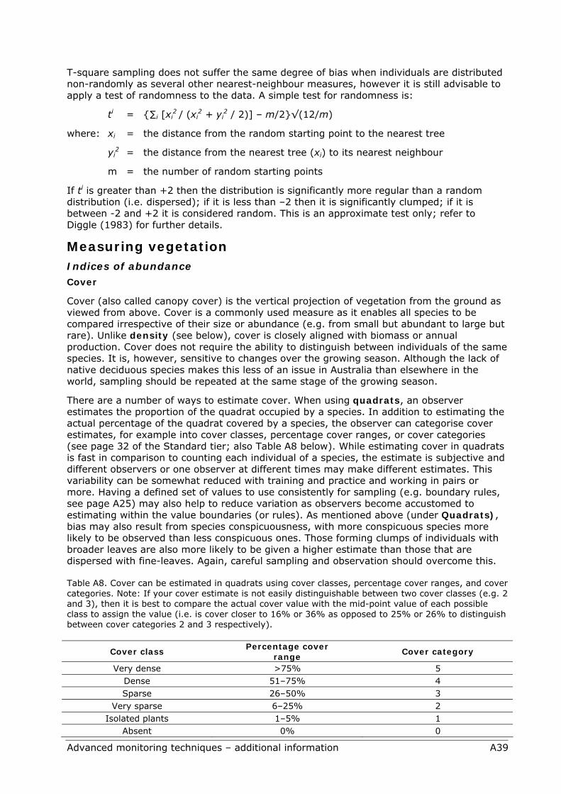
Table A8. Cover can be estimated in quadrats using cover classes, percentage cover ranges, and cover categories. Note: If your cover estimate is not easily distinguishable between two cover classes (e.g. 2 and 3), then it is best to compare the actual cover value with the mid-point value of each possible class to assign the value (i.e. is cover closer to 16% or 36% as opposed to 25% or 26% to distinguish between cover categories 2 and 3 respectively).

Cover class Percentage cover

range Cover category

Very dense >75% 5 Dense 51–75% 4 Sparse 26–50% 3

Very sparse 6–25% 2 Isolated plants 1–5% 1

Absent 0% 0

A40 Monitoring manual for bitou bush control and native plant recovery

Compared with quadrats, cover measured using line-intercept transects is objective and variation between observers is greatly reduced. Care should be taken, however, if permanent transects are being used, as it is more difficult to measure the exact same line-intercept transect each time than measuring a permanent quadrat with all four corners marked out. Changes in the tape tension, blowing in the wind for example, and slightly different placement because of obstacles are examples of factors which may reduce your ability to re-measure the same transect. Failure to intersect a particular plant on a subsequent measurement can therefore result from 1) tape movement and missing the exact location, 2) decline in cover of the plant so that your tape no longer intersects it, and 3) death (or dormancy) of the plant. Only the first is a problem, the others are normal biological occurrences. It would not be practical to use this method in an area of dense brush and undergrowth as this would make it very unlikely that you re-measure the same line. To reduce the chances of not re-measuring the same transect line, it can be permanently marked with a star picket at each end and at intermediate positions along the transect (e.g. at 5 or 10 m intervals). Shorter transects will also reduce issues such as the tape sagging.

For all methods it should also be noted that overlapping cover of individuals of the same species should not be counted twice, but should be recorded as continuous cover. If however, two or more different plant species overlap then the cover of each species should be recorded separately; this may give more than 100% cover if there are many overlapping canopies.

Note: In addition to measuring the cover of plant species, you can also measure the cover of bare ground or leaf litter, and that of different life history categories. These variables are important in some ecological communities.

Density

Density is the number of individuals per unit area. For plants, it is generally calculated as the number of individual plants per metre square or per hectare. Because it is a per-area measure, density estimates can be compared across sampling units, even if the size and shape of sampling units vary.

Density can only be calculated if individual plants are readily and consistently identifiable. Density measurements are not suitable if plants form dense mats or clumps due to the difficulty of distinguishing between plants. Density will also be impractical for very sparsely distributed or rare species. Conversely, counting many individuals for density can be very time consuming and difficult unless you use very small quadrats. Note also that, like cover estimates, density estimates can be biased towards more conspicuous species.

Density estimates will detect changes in abundance via recruitment or mortality. They are unable, however, to detect changes in condition, for example new growth or a decline in foliage or health. In addition to estimating the overall density of plants within an area, the density of different life history categories (e.g. seedlings, juveniles, and adults; reproductive or non-reproductive) can also be calculated. These estimates provide more sensitivity to some changes in the population.

Presence/absence

Presence/absence is a simple record of whether a species is found within a sampling unit or not (this will also result in a floristic survey, except where you have a targeted list of species you wish to sample). The key advantage of this method is that no special skills are required, other than the ability to identify the species. This technique is also very fast, although care must be taken to search thoroughly for all species (or a select list of species you are interested in, e.g. the target species). Presence/absence is insensitive to changes other than the appearance or complete disappearance of a species from a sampling unit.

Advanced monitoring techniques – additional information A41

Therefore, while presence/absence provides information on species richness within a sampling unit, it provides no further information on the abundance, cover, density or diversity of species.

Demographic measures Life history dynamics

Measures of the life history dynamics of a target species (e.g. the percent cover and/or the number of seedling, juvenile, adult, and dead plants) should be used to supplement general measures of cover and density. Measuring the life history dynamics of a species is much more time consuming than straight estimates of cover or density for the species as a whole. However, recording the life history dynamics of target species provides detailed information on the effectiveness of your control methods on the weed species (e.g. adult plants are killed but there is seedling recruitment) and the recovery of native species (e.g. if the increased cover is because adult plants are growing or if there is seedling recruitment). As a minimum, you could separate a species into seedling and non-seedling classes.

You can choose to record the life history dynamics of your target species using cover or density estimates, however these two measures give quite different results. If using cover, you will record the proportion of your plot that is covered by each life history category. Note: If you have overlapping layers then the sum of cover values for all four life history categories combined may be more than the overall percentage cover. This will occur, for example, if you have seedlings growing underneath an adult plant. In contrast, density estimates are the estimated number of individuals in your plot in each of the four life history categories. Details for recording life history dynamics are provided in the relevant section for each of the methods.

Diameter at breast height (DBH)

Diameter at breast height (DBH) is a standard method of measuring the diameter of trees or shrubs. It is measured at 1.3 m above ground level, and on the uphill side if the plant is on a slope. DBH can be measured using callipers, or a tape measure to record the circumference; the diameter is calculated by dividing the circumference by pi (π: 3.14159).

Height

Measuring the height of a plant gives you an additional measure of vigour. You can either measure the height of the tallest individual of a target species in your plot, or you can measure the average height of that species in your plot; if you are measuring the average height then you should measure the height of at least five randomly chosen individuals. Whether you measure the maximum or average height will of course give you different information about a target species. To decide which one to measure (although you can measure both), you should think about the likely changes a species will make after control, and how this measure fits with the aim of your monitoring program.

The heights of small shrubs and groundcover species (e.g. grasses) are easily measured or estimated, however trees are more difficult. Two methods to estimate tree height are outlined below.

Using a clinometer 1. Stand on the same contour as the bottom of the tree (while there is no pre-determined

distance you must stand away from the tree, you must be able to see both the top and bottom of the tree easily) and measure the angle from the horizontal (eye-height on the tree) to the top of the tree using a clinometer (e.g. θ = 38°; Figure A22).

2. Measure the horizontal distance from you to the tree (in Figure A22, for example, this distance ‘x’ equals 20 m).

3. Use trigonometry (on your calculator or a statistical program such as Excel) to calculate the height of the tree, minus your eye-height (distance ‘y’ in Figure A22).

4. Add the height of your eyes above ground level to ‘y’ to calculate the total height of the tree. In Figure A22 this is 1.6 m.

A42 Monitoring manual for bitou bush control and native plant recovery

y = 15.6 m

θ = 38o

1.6 mx = 20 m

17.2 m

Figure A22. An example of how to estimate the height of a tree using a clinometer and trigonometry.

For example, to calculate the height of the tree in Figure A22 you need to calculate the distances ‘x’ and ‘y’, and the angle θ. Measure distance ‘x’ using a tape measure and the angle θ using a clinometer; use trigonometry to calculate ‘y’. Using the formula below, you know that x = 20 m and θ = 38°:

Solving this formula for ‘y’ gives you a value of 15.6 m. Add the height of your eyes above ground level (1.6 m) to the distance ‘y’ to calculate the total tree height: total tree height = 1.6 m + 15.6 m = 17.2 m.

Therefore, the height of the tree in Figure A22 is approximately 17.2 m.

Using a stick

1. Mark a stick or ruler 10% along its length (e.g. at the 3 cm mark for a 30 cm ruler; Figure A23).

2. Walk away from the tree until the top and bottom of the stick line up with the top and bottom of the tree (Figure A23). There is no need to stay on the same contour as the tree.

1.7 m

17 m30 cm ruler

10% mark on ruler (3 cm)

10% mark on tree (1.7 m)

Figure A23. An example of how to estimate the height of a tree using a stick.

θadjacent side = x

hypotenuse = z

oppo

site

sid

e =

y

θθadjacent side = x

hypotenuse = z

oppo

site

sid

e =

y oppositetan θ = = adjacent

yxyx

ytan 38 = 20

y = 20(tan 38) ≈ 15.6

Advanced monitoring techniques – additional information A43

3. Mark the point on the tree which corresponds to the 10% mark on the stick; measure the height of this point above ground level (e.g. 1.7 m above ground level; Figure A23).

4. To calculate the total height of the tree, multiply this measurement by 10. For example, if the 10% mark aligns with a point 1.7 m above ground level, then the total tree height = 1.7 m x 10 = 17 m.

Reproductive status

The flowering (particularly age at first flowering) and fruiting times and the timing of vegetative reproduction are still unknown for many species, so any such reproductive information will be useful. This data also provides an additional measure of the recovery of native species after weed control, and the interval at which weed control is needed for perennial weed species (e.g. before first flowering of the weed species). Such data is also useful for determining the rate at which native species may re-establish seedbanks, by providing information about their time to first flowering and seed set.

Species richness

Species richness is an index of the number of species within a sampling unit. It provides a simple indication of how weed species are affecting species abundance, and whether there is an increase in overall species abundance following weed control. Although conceptually simple, species richness relies on a full floristic survey of the sampling unit, and care must be taken to identify all the species within the sampling unit. It may be difficult to calculate species richness if 1) there are a large number of species, 2) many species are rare, 3) species are cryptic or absent above ground at certain times of the year (e.g. orchids), or 4) the vegetation is dense, making it difficult to assess all areas of the sampling unit.

Species richness can mask important differences in the abundance of different species, however. For example, a quadrat containing one dominant species and 19 rare species is very different to a quadrat containing 20 species with similar abundance, yet it has the same species richness (20 species).

Species diversity

Species diversity is a measure of the ‘evenness’ of species. Species diversity incorporates a measure of species richness, however it also provides additional information on community health by providing an index of the abundance of the range of species present within a community. A diversity index will indicate, for example, whether a community is dominated by only one species with all other species being relatively rare, or whether the abundance of all species is relatively even (see the example below, Figure A24).

There are many different diversity indices, each with their proponents and detractors (see Ludwig and Reynolds 1988, Magurran 1988, Krebs 1998). A commonly used species diversity index is the Shannon index (H'):

S = the number of species (also called species richness) pi = the relative abundance of each species, calculated as the proportion

of individuals of a given species to the total number of individuals (of all species) in the community (ni /N)

ni = the number of individuals of species i

where

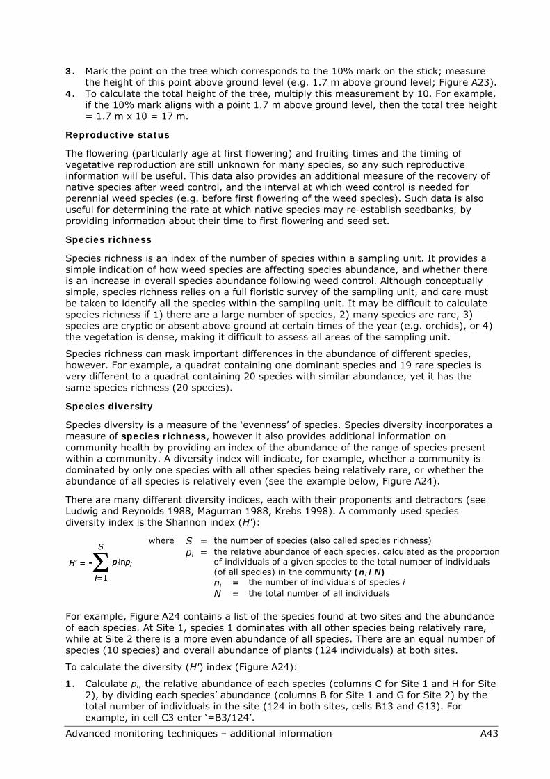
N = the total number of all individuals For example, Figure A24 contains a list of the species found at two sites and the abundance of each species. At Site 1, species 1 dominates with all other species being relatively rare, while at Site 2 there is a more even abundance of all species. There are an equal number of species (10 species) and overall abundance of plants (124 individuals) at both sites.

To calculate the diversity (H') index (Figure A24):

1. Calculate pi, the relative abundance of each species (columns C for Site 1 and H for Site 2), by dividing each species’ abundance (columns B for Site 1 and G for Site 2) by the total number of individuals in the site (124 in both sites, cells B13 and G13). For example, in cell C3 enter ‘=B3/124’.

ΣS

pilnpiH’ =

i=1

-ΣS

pilnpiH’ =

i=1

-

A44 Monitoring manual for bitou bush control and native plant recovery

2. Multiply each value of pi (columns C for Site 1 and H for Site 2) by the natural log (ln) of pi (vales in columns D for Site 1 and I for Site 2). For example, in cell D3 enter ‘=C3*ln(C3)’.

3. Sum these values for all species and multiply the sum by i (or –1) (cell D13 for Site 1 and cell I13 for Site 2). For example, in cell D13 enter ‘=–1*SUM(D3:D12)’.

Figure A24. An example of how to calculate the H' index for two sites.

These calculations give an H' index of 0.82 for Site 1, and 2.29 for Site 2. Site 2 can therefore be said to have higher species diversity than Site 1, although both sites have an equal number of species (species richness, ten species at each site) and an overall equal number of individuals (124 individuals).

Measuring response to control

Information on the response of native species to accidental (off-target) herbicide application is limited to a relatively small number of species (Toth & Winkler 2008). Recording the status of native species after control will supplement what is already known, which will be useful for the wider community, as well as for interpreting your own results.

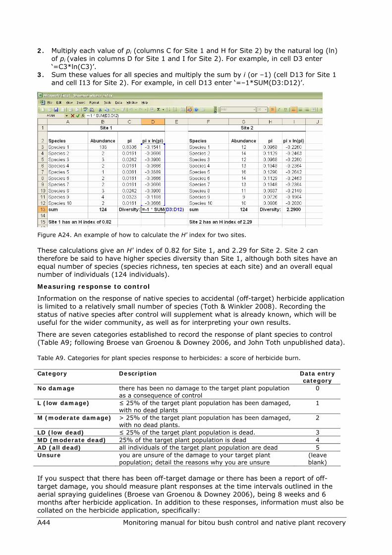
There are seven categories established to record the response of plant species to control (Table A9; following Broese van Groenou & Downey 2006, and John Toth unpublished data).

Table A9. Categories for plant species response to herbicides: a score of herbicide burn.

Category Description Data entry category

No damage there has been no damage to the target plant population as a consequence of control

0

L (low damage) ≤ 25% of the target plant population has been damaged, with no dead plants

1

M (moderate damage) > 25% of the target plant population has been damaged, with no dead plants.

2

LD (low dead) ≤ 25% of the target plant population is dead. 3 MD (moderate dead) 25% of the target plant population is dead 4 AD (all dead) all individuals of the target plant population are dead 5 Unsure you are unsure of the damage to your target plant

population; detail the reasons why you are unsure (leave blank)

If you suspect that there has been off-target damage or there has been a report of off-target damage, you should measure plant responses at the time intervals outlined in the aerial spraying guidelines (Broese van Groenou & Downey 2006), being 8 weeks and 6 months after herbicide application. In addition to these responses, information must also be collated on the herbicide application, specifically:

Advanced monitoring techniques – additional information A45

the herbicide and application rate the interval between application and the observation (e.g. 3 months) a follow-up sample to determine long-term response.

Understanding experimental design A number of important sampling considerations when designing a monitoring program were outlined on page A4. These sampling issues are described in more detail below.

Unbiased sampling Unbiased sampling (also known as random sampling) forms the basis of most statistical techniques. Non-random samples cannot be used to make statistical inferences about your population. Subjective sampling units should therefore be avoided. This does not mean that you cannot stratify (see page A48) your sampling design to target specific species or ecological communities, but that within strata there must be some form of unbiased sampling. There are several methods of unbiased sampling, two of which are recommended below.

Random sampling

The locations of all sampling units are selected randomly. Simple random sampling is useful in relatively small geographic areas with homogenous habitats when temporary quadrats are used. When permanent quadrats are used, simple random sampling can be used over larger areas. Random quadrat sampling does not perform very well when populations have a clumped distribution, and the time taken to determine the random locations and setting up plots can be considerable. Note also that, by chance, some areas within the target population may be left unsampled.

Systematic sampling

Systematic sampling uses a randomly selected starting point as the location of the first sampling unit, with subsequent sampling units placed at regular distances from the starting point. A common form of systematic sampling is the regular placement of quadrats along a transect. A systematic sampling design is recommended when sampling clumped distributions and is commonly used for sampling plant populations. Several advantages of systematic sampling are short set-up times, good interspersion of sampling units (see page A46), and more efficient location of systematically distributed sampling units versus randomly distributed sampling units. It is important that systematic sampling units are independent of one another. Guidelines for minimum distances between systematic sampling units were provided on page A4.

There is some evidence that systematic sampling is more representative than random sampling, primarily because the sampling units are spread evenly throughout the study area (interspersion). However, systematic sampling only allows an estimation of the sampling error if the objects being sampled (e.g. the individuals of a target species) are assumed to be in random order. Systematic sampling is invalid and biased if the unit of repetition (e.g. the distance between systematic sampling units) follows some natural repetition in the distribution of objects being sampled. If, for example, the distance between systematic quadrats along a transect is equivalent to the distance between dune swales, then the same area of a swale would be sampled repetitively and sampling would not provide data on i) the overall vegetation found across dunes or ii) the inter-swale vegetation. If the objects being sampled are distributed randomly, however, then a systematic sample can be treated as being effectively a simple random sample.

The systematic sampling methods outlined in this manual all use the individual sampling unit (e.g. the individual quadrats or sub-transects) as the unit of replication. It is possible, however, to consider the transect upon which these sub-units are placed as the sampling unit. Your choice of sampling unit will affect average and standard error calculations, and of course any further analyses. For example, systematic data can be analysed with the quadrats as the sampling unit (e.g. Figure A25), or by considering the transects as the sampling unit (e.g. Figure A26). In Figure A26, the average for each transect must first be

A46 Monitoring manual for bitou bush control and native plant recovery

calculated (e.g. the average of cells D16:D20 for Transect 1 in D32, D21:D25 for Transect 2 in D33, and D26:D30 for Transect 3 in D34). The monitoring event average and standard error is then calculated from these values (e.g. cells D32:D34).

Figure A25. An example of systematic quadrat sampling where the quadrats (sub-units) are considered the unit of replication.

Figure A26. An example of systematic quadrat sampling where the transects are considered the unit of replication.

A quick comparison shows that the monitoring event averages (e.g. row 32 for Figure A25 and row 36 for Figure A26) are very similar for the two methods, however the standard errors (e.g. row 33 for Figure A25 and row 37 for Figure A26) are mostly larger when the quadrats (sub-units) are the unit of replication (Figure A25), than when the transects are the unit of replication (Figure A26).

Your decision to consider the sub-units or entire transects as the sampling unit should depend on the aim and design of your monitoring program.

Interspersion Interspersion refers to the distribution of sampling units throughout your site. In a robust sampling design, sampling units should be well dispersed throughout the site. To ensure interspersion, you should avoid placing all sampling units along a single (or only a few) transects, even if these have been randomly located.

Advanced monitoring techniques – additional information A47

Independence Independence means that the sampling units are placed far enough apart so that measurements are not spatially correlated, i.e. that what happens in one quadrat will not affect what happens in another simply because they are located near one another. You must take care when selecting the spacing of systematic samples to ensure independence; see page A4 for guidance.

Replication Lack of replication in sampling is identified as one of the most common mistakes that occur. Replication is essential to ensure comparisons can be made both spatially and temporally. A single sample unit provides an imprecise estimate for the whole study population and, no matter how carefully or randomly chosen, might not be representative. To overcome this, more than one sampling unit is required. Replication allows you to measure the precision of the generalisations you make in your study, e.g. average number of a target species in all 20 plots, and also enables the use of standard errors or confidence limits. Tables A5 and A6 provide some advice on the minimum number of samples required to provide adequate replication for each method. Note that the level of replication referred to in this tier is that within a site. As sampling units are not replicated across sites, no generalisations can be made away from the site that is monitored.

Some other important experimental design considerations when designing a monitoring program are whether to have permanent or temporary sampling units, or to stratify your sampling units.

Permanent vs temporary sampling The decision to have either permanent or temporary sampling is a critical one that affects almost all other aspects of your monitoring.

Temporary sampling

Temporary sampling involves the placement of new plots each sampling period. For example, if sampling to detect a change in a plant species density over time then in the first year you would randomly select locations for twenty quadrats within your monitoring site and count the number of species in each quadrat (adhering to your boundary rule; see page A25). In the second year of sampling you would randomly select another twenty (new) locations for your quadrats and count the number of species in each quadrat. The quadrats in this example are temporary and the two samples are independent of each other in both space and time.

Permanent sampling

A permanent sampling procedure can also be used with the same sampling objective, i.e. to detect a change in a plant species density over time. For example, in the first year of sampling you randomly select the twenty locations as above and count the number of individuals in each quadrat. However, instead of selecting new quadrat locations each year, in the first year you permanently mark the locations of the quadrats, typically both physically using star pickets or another type of marker, and spatially with a handheld GPS unit. In the second year of sampling you would count the individuals in the same quadrats as for the first year. In this example the sampling quadrats are permanent and the two samples are dependent in space, but are independent in time.

The main advantage of using permanent instead of temporary sampling is that for many species the statistical tests for detecting change from one period to the next in permanent plots are much more powerful than for those used for temporary plots. This translates into a reduction in the number of sampling units that must be sampled to detect a certain magnitude of change. Permanent plots can also help to reduce the time spent monitoring because although initially intensive to set up, permanently marked plots need only be located at subsequent sampling events. Conversely, when using temporarily marked plots, the location of new temporary plots must be determined and plot boundaries delineated in each sampling period before monitoring can begin.

A48 Monitoring manual for bitou bush control and native plant recovery

Stratified sampling Stratification involves dividing the monitoring area into non-overlapping areas (strata), and selecting a simple random sample (or samples) from each of the strata. Stratified sampling is appropriate if there is some underlying structure to the population, for example if different soil types result in different communities, if fires have burnt some patches of vegetation but not others, or if the units to be sampled are not distributed evenly throughout the study area. Some common methods of stratification include spatial location, such as altitude, vegetation type, and the soil type. The population is expected to be uniform within each strata. There is a natural tendency to stratify sampling according to vegetation type, for example few people would combine monitoring results of Themeda grasslands with littoral rainforest and expect them to be comparable. In some instances, however, care needs to be taken that the study area is suitably stratified, for example into areas with different fire histories.

There are numerous benefits to stratified sampling. Stratified samples will have a smaller standard error than those obtained with a simple random sample if the individuals within strata are more similar than individuals in general. Benefits can also arise from having separate estimates of population parameters for the different strata. By stratifying, you can also sample different parts of a population in different ways, potentially saving time and money (Manly 1992).

Considerations when selecting sampling units Size, shape and number of sampling units The ideal size, shape and number of sampling units to use will depend on the size and density of individuals within the community being sampled and your purpose in monitoring.

Size

Sampling units must be large enough to contain a number of individuals, but small enough that the individuals present can be separated, counted and measured. The ideal dimensions and number of sampling units will therefore vary between vegetation growth forms.

Shape

Most of the literature for sampling design recommends the use of rectangular quadrats as opposed to square or circular quadrats. For sampling bitou bush and native species, we also recommend rectangular quadrats, particularly those that are ≤2 m wide as this will allow you to measure plants from the boundary and therefore reduce the trampling within your quadrats. However, the decision on size and shape will depend on your vegetation type and the species you are targeting.

Sampling unit dimensions are prescribed in the Advanced tier (see Tables A5 and A6), however a wide range of other dimensions are also valid. Table A10 provides you with some suggested quadrat dimensions for different vegetation categories. This takes into account the type of growth form of the plant but also time constraints in sampling. For most plants other than herbaceous growth forms, the larger the quadrat size the better.

Number

The number of sampling units you use is central to your ability to answer your monitoring question(s). A number of points should be considered when deciding upon a sample size:

It should be driven by your monitoring objectives. Generally, more rigorous, scientific studies will require more replicates than those looking for general trends.

It should be based on the variability in the measurements, which should be determined via a pilot study (see below).

Your selection of sample size should also be based upon the time and resources you have available to commit to monitoring over the anticipated life of the project. If you are unable to commit sufficient resources to monitoring a sample size that will answer your monitoring question, then your monitoring question should be changed and the required sample size re-calculated.

Advanced monitoring techniques – additional information A49

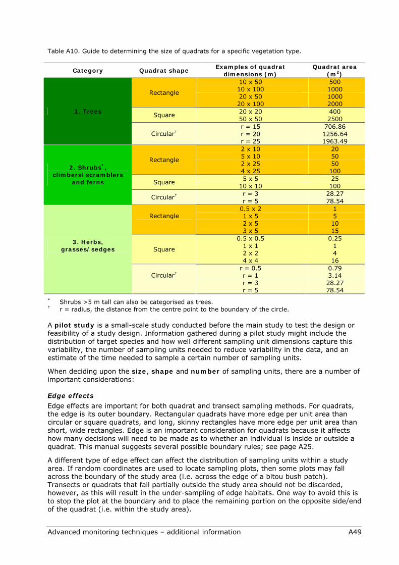
Table A10. Guide to determining the size of quadrats for a specific vegetation type.

Category Quadrat shape Examples of quadrat

dimensions (m) Quadrat area

(m2) 10 x 50 500 10 x 100 1000 20 x 50 1000

Rectangle

20 x 100 2000 20 x 20 400 Square 50 x 50 2500 r = 15 706.86 r = 20 1256.64

1. Trees

Circular† r = 25 1963.49 2 x 10 20 5 x 10 50 2 x 25 50

Rectangle

4 x 25 100 5 x 5 25 Square

10 x 10 100 r = 3 28.27

2. Shrubs*, climbers/scramblers

and ferns

Circular† r = 5 78.54

0.5 x 2 1 1 x 5 5 2 x 5 10

Rectangle

3 x 5 15 0.5 x 0.5 0.25

1 x 1 1 2 x 2 4

Square

4 x 4 16 r = 0.5 0.79 r = 1 3.14 r = 3 28.27

3. Herbs, grasses/sedges

Circular†

r = 5 78.54 * Shrubs >5 m tall can also be categorised as trees. † r = radius, the distance from the centre point to the boundary of the circle.

A pilot study is a small-scale study conducted before the main study to test the design or feasibility of a study design. Information gathered during a pilot study might include the distribution of target species and how well different sampling unit dimensions capture this variability, the number of sampling units needed to reduce variability in the data, and an estimate of the time needed to sample a certain number of sampling units.

When deciding upon the size, shape and number of sampling units, there are a number of important considerations:

Edge effects Edge effects are important for both quadrat and transect sampling methods. For quadrats, the edge is its outer boundary. Rectangular quadrats have more edge per unit area than circular or square quadrats, and long, skinny rectangles have more edge per unit area than short, wide rectangles. Edge is an important consideration for quadrats because it affects how many decisions will need to be made as to whether an individual is inside or outside a quadrat. This manual suggests several possible boundary rules; see page A25.

A different type of edge effect can affect the distribution of sampling units within a study area. If random coordinates are used to locate sampling plots, then some plots may fall across the boundary of the study area (i.e. across the edge of a bitou bush patch). Transects or quadrats that fall partially outside the study area should not be discarded, however, as this will result in the under-sampling of edge habitats. One way to avoid this is to stop the plot at the boundary and to place the remaining portion on the opposite side/end of the quadrat (i.e. within the study area).

A50 Monitoring manual for bitou bush control and native plant recovery

Ease in sampling The size and shape of your sampling unit will affect the ease with which it can be sampled. In a large square quadrat, for example, it may be difficult to keep track of which individuals you have and have not counted, and you may need to subdivide the large quadrat into several smaller quadrats. For this reason, long, narrow quadrats are often easier to search.

Abundance of target population Smaller quadrats are better if the density of individuals is high – this will save you counting data on hundreds or thousands of individuals. Conversely, if the density of individuals is low then larger quadrats will avoid sampling many quadrats with no individuals.

Travel and set up time versus searching and measuring time The terrain and vegetation at a site can have an enormous effect on the time it takes to set up and travel between sampling units, and also the time taken to search within units and conduct monitoring. There are several factors you should consider when designing your monitoring program:

The time required to measure a sampling unit will increase with the size of the sampling unit.

The time required to set up sampling units will increase with vegetation density, the size of sampling units, and terrain complexity.

The travel time between units will increase with vegetation density, terrain complexity, and the distance between sampling units.

The difficulty of locating permanent quadrats and transects will increase with vegetation density and the distance between sampling units.

Spatial distribution of individuals in the population Few species are distributed randomly in space; most are instead aggregated or clumped in their distribution (though some are dispersed). The distribution of a species should affect the size and shape of the sampling unit you select. You should aim to use sampling units that intersect some clumps of a species you are interested in, as this will reduce the number of units with zero counts, and the number of units with very high counts. The sampling unit length (e.g. the length of a transect or the length of the long side of a quadrat) should ideally be longer than the mean distance between clumps of a species.

When orienting sampling units, you should also consider the presence of physical (e.g. slope, soil type, elevation, distance from salt source) or biological (e.g. density, diversity) gradients in the population. Transects or rectangular quadrats should be positioned so that they run parallel with any gradients, as the variation along the gradient will then be captured within sampling units rather than between them. This results in lower variability between sampling units.

You may consider doing a pilot study to assess the above considerations before you establish final sampling methods for the rest of your study.

Disturbance effects from monitoring You should consider what effects your presence might have on the species you are monitoring, for example through trampling. This is especially important when sampling units are permanent, as your repeated visits can impact the population independent to the treatments you are trying to monitor.