Advanced Mathematical Models and Methods - vse.cznb.vse.cz/~fabry/POR-prezentace.pdf · Jan Fábry...
150
Advanced Mathematical Models and Methods Jan Fábry ŠKODA AUTO University Department of Logistics, Quality and Automotive Technology [email protected] http://nb.vse.cz/~fabry November 10, 2017, Mladá Boleslav Jan Fábry Advanced Mathematical Models and Methods 1 / 150
-
Upload
vuongkhanh -
Category
Documents
-
view
219 -
download
0
Transcript of Advanced Mathematical Models and Methods - vse.cznb.vse.cz/~fabry/POR-prezentace.pdf · Jan Fábry...

Advanced Mathematical Models and Methods
Jan Fábry
ŠKODA AUTO UniversityDepartment of Logistics, Quality and Automotive Technology
[email protected]://nb.vse.cz/~fabry
November 10, 2017, Mladá Boleslav
Jan Fábry Advanced Mathematical Models and Methods 1 / 150

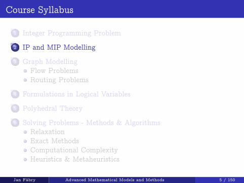
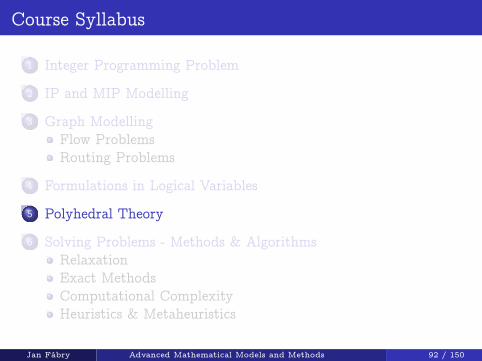
Course Syllabus
1 Integer Programming Problem
2 IP and MIP Modelling
3 Graph ModellingFlow ProblemsRouting Problems
4 Formulations in Logical Variables
5 Polyhedral Theory
6 Solving Problems - Methods & AlgorithmsRelaxationExact MethodsComputational ComplexityHeuristics & Metaheuristics
Jan Fábry Advanced Mathematical Models and Methods 2 / 150

Course Syllabus
1 Integer Programming Problem
2 IP and MIP Modelling
3 Graph ModellingFlow ProblemsRouting Problems
4 Formulations in Logical Variables
5 Polyhedral Theory
6 Solving Problems - Methods & AlgorithmsRelaxationExact MethodsComputational ComplexityHeuristics & Metaheuristics
Jan Fábry Advanced Mathematical Models and Methods 3 / 150

Integer Programming Problem
General linear programming problem (LP):
zLP = maxfcTx : Ax � b; x 2 Rn+g: (1)
Integer programming problem (IP):
zIP = maxfcTx : Ax � b; x 2 Zn+g: (2)
zLP � zIP since Zn+ � Rn
+P = fx : Ax � b; x 2 Rn
+g;S = fx : Ax � b; x 2 Zn+g;S � P
Mixed integer programming problem (MIP):
zMIP = maxfcTx + hTy : Ax +Gy � b; x 2 Rn+; y 2 Zp
+g: (3)
Binary integer programming problem (BIP):
zBIP = maxfcTx : Ax � b; x 2 Bng;B = f0; 1g: (4)
Jan Fábry Advanced Mathematical Models and Methods 4 / 150
Course Syllabus
1 Integer Programming Problem
2 IP and MIP Modelling
3 Graph ModellingFlow ProblemsRouting Problems
4 Formulations in Logical Variables
5 Polyhedral Theory
6 Solving Problems - Methods & AlgorithmsRelaxationExact MethodsComputational ComplexityHeuristics & Metaheuristics
Jan Fábry Advanced Mathematical Models and Methods 5 / 150

IP and MIP Modelling
1. Production Planning ProblemVariables: xi is a number of pcs. of i -th productConstraints: x1; x2; : : : ; xn are integers
2. Cutting Stock ProblemVariables: xi is a number of pcs. of raw products being cutaccording to i -th cutting patternConstraints: x1; x2; : : : ; xn are integersThe objective:
Minimization of pcs. of cut raw productsMinimization of total wasteMaximization of pcs. of assembled products (profit)
Jan Fábry Advanced Mathematical Models and Methods 6 / 150

IP and MIP Modelling
3. (0-1) Knapsack ProblemDefinition: Budget b is available for investments in n consideredprojects, where aj is the outlay for project j and cj is its expectedreturn. The objective is to choose a set of projects to maximize thetotal expected return while not exceeding the budget.Variables:
xj =
(1 if the project j is selected0 otherwise
(5)
Model:max
nXj=1
cj xj (6)
nXj=1
aj xj � b (7)
xj 2 f0; 1g for j = 1; 2; : : : ;n (8)
Jan Fábry Advanced Mathematical Models and Methods 7 / 150

IP and MIP Modelling
4. Perfect Matching ProblemDefinition: On a trip, n (even number) students are to be assignedto double rooms. Satisfaction value cij is given for potentialroommates i and j . The objective is to assign students tomaximize the total satisfaction of the group.Variables:
xij =
(1 if students i and j are roommates0 otherwise
i < j (9)
Model:max
n�1Xi=1
nXj=i+1
cij xij (10)
Xj<i
xji +Xj>i
xij = 1 for i = 1; 2; : : : ;n (11)
xij 2 f0; 1g fori = 1; 2; : : : ;n � 1j = i + 1; i + 2; : : : ;n
(12)
Jan Fábry Advanced Mathematical Models and Methods 8 / 150

IP and MIP Modelling
5. Generalized Assignment ProblemDefinition: Let us assume m stations taking petrol fromn terminals. Each station i can take petrol exactly from oneterminal and its requirement ai is given. Capacity of terminal j isdenoted by bj . If station i takes petrol from terminal j then costcij is calculated. The objective is to minimize the total cost.Variables:
xij =
(1 if station i takes petrol from terminal j0 otherwise
(13)
Jan Fábry Advanced Mathematical Models and Methods 9 / 150

IP and MIP Modelling
5. Generalized Assignment ProblemModel:
minmXi=1
nXj=1
cij xij (14)
nXj=1
xij = 1 for i = 1; 2; : : : ;m (15)
mXi=1
aixij � bj for j = 1; 2; : : : ;n (16)
xij 2 f0; 1g fori = 1; 2; : : : ;mj = 1; 2; : : : ;n
(17)
Jan Fábry Advanced Mathematical Models and Methods 10 / 150

IP and MIP Modelling
6. Linear Assignment ProblemDefinition: There are n people available to carry out n jobs. Eachperson is assigned to carry out exactly one job. Some individualsare better suited to particular jobs than others, so there is anestimated cost cij if person i is assigned to job j . The objective isto find a minimum cost assignment.Variables:
xij =
(1 if person i does job j0 otherwise
(18)
Jan Fábry Advanced Mathematical Models and Methods 11 / 150

IP and MIP Modelling
6. Linear Assignment ProblemModel:
minnXi=1
nXj=1
cij xij (19)
nXj=1
xij = 1 for i = 1; 2; : : : ;n (20)
nXi=1
xij = 1 for j = 1; 2; : : : ;n (21)
xij 2 f0; 1g fori = 1; 2; : : : ;nj = 1; 2; : : : ;n
(22)
Jan Fábry Advanced Mathematical Models and Methods 12 / 150
IP and MIP Modelling
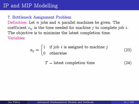
7. Bottleneck Assignment ProblemDefinition: Let n jobs and n parallel machines be given. Thecoefficient cij is the time needed for machine j to complete job i .The objective is to minimize the latest completion time.Variables:
xij =
(1 if job i is assigned to machine j0 otherwise
(23)
T = latest completion time (24)
Jan Fábry Advanced Mathematical Models and Methods 13 / 150

IP and MIP Modelling
7. Bottleneck Assignment ProblemModel:
min T (25)
cij xij � T fori = 1; 2; : : : ;nj = 1; 2; : : : ;n
(26)
nXj=1
xij = 1 for i = 1; 2; : : : ;n (27)
nXi=1
xij = 1 for j = 1; 2; : : : ;n (28)
xij 2 f0; 1g fori = 1; 2; : : : ;nj = 1; 2; : : : ;n
(29)
Jan Fábry Advanced Mathematical Models and Methods 14 / 150

IP and MIP Modelling
8. Quadratic Assignment ProblemDefinition: A set of n facilities has to be allocated to a set ofn locations. The coefficient cij is the flow from facility i to facilityj and the value dkl is the distance from location k to location l .The objective is to allocate each facility to a location such that thetotal cost is minimized.Variables:
xik =
(1 if facility i is assigned to location k0 otherwise
(30)
Jan Fábry Advanced Mathematical Models and Methods 15 / 150

IP and MIP Modelling
8. Quadratic Assignment ProblemModel:
minnXi=1
nXj=1
nXk=1
nXl=1
cijdklxikxjl (31)
nXk=1
xik = 1 for i = 1; 2; : : : ;n (32)
nXi=1
xik = 1 for k = 1; 2; : : : ;n (33)
xik 2 f0; 1g fori = 1; 2; : : : ;nk = 1; 2; : : : ;n
(34)
Jan Fábry Advanced Mathematical Models and Methods 16 / 150

IP and MIP Modelling
8. Quadratic Assignment ProblemLinearization of the objective function:
yijkl =
8>><>>:1 if facility i is assigned to location k
and facility j is assigned to location l0 otherwise
(35)
minnXi=1
nXj=1
nXk=1
nXl=1
cijdklyijkl (36)
yijkl � xik + xjl � 1 for i ; j ; k ; l = 1; 2; : : : ;n (37)
Jan Fábry Advanced Mathematical Models and Methods 17 / 150

IP and MIP Modelling
8. Quadratic Assignment ProblemApplications:
Placement Problem
The Airport Gate Assignment Problem
Jan Fábry Advanced Mathematical Models and Methods 18 / 150
IP and MIP Modelling
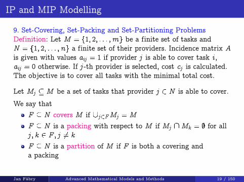
9. Set-Covering, Set-Packing and Set-Partitioning ProblemsDefinition: Let M = f1; 2; : : : ;mg be a finite set of tasks andN = f1; 2; : : : ;ng a finite set of their providers. Incidence matrix Ais given with values aij = 1 if provider j is able to cover task i ,aij = 0 otherwise. If j -th provider is selected, cost cj is calculated.The objective is to cover all tasks with the minimal total cost.
Let Mj �M be a set of tasks that provider j 2 N is able to cover.
We say thatF � N covers M if [j2FMj =MF � N is a packing with respect to M if Mj \Mk = ; for allj ; k 2 F ; j 6= kF � N is a partition of M if F is both a covering anda packing
Jan Fábry Advanced Mathematical Models and Methods 19 / 150

IP and MIP Modelling
9. Set-Covering, Set-Packing and Set-Partitioning ProblemsVariables:
xj =
(1 if provider j is selected, i.e. j 2 F0 otherwise
(38)
Model:min
nXj=1
cj xj (39)
(set-covering)nX
j=1
aij xj � 1 for i = 1; 2; : : : ;m
(set-packing)nX
j=1
aij xj � 1 for i = 1; 2; : : : ;m
(set-partitioning)nX
j=1
aij xj = 1 for i = 1; 2; : : : ;m
(40)
xj 2 f0; 1g for j = 1; 2; : : : ;n (41)
Jan Fábry Advanced Mathematical Models and Methods 20 / 150

IP and MIP Modelling
9. Set-Covering, Set-Packing and Set-Partitioning ProblemsApplications:
Let N = f1; 2; : : : ;ng be a set of potential sites for thelocation of fire stations. A station placed at j costs cj . LetM = f1; 2; : : : ;mg be a set of communities that have to beprotected. The subset of communities that can be protectedfrom j (e.g. reached from the fire station in 10 minutes) is Mj .Assigning airline crews to flights.Scheduling workers to shifts.
Jan Fábry Advanced Mathematical Models and Methods 21 / 150

IP and MIP Modelling
10. Facility Location ProblemDefinition: A set of potential depots M = f1; 2; : : : ;mg and a setof clients N = f1; 2; : : : ;ng are given. Suppose a facility located ati has a capacity of ai and the j -th client has demand bj . Fixed costfi is associated with the use of depot i and transportation cost cijis charged for shipping unit between location i and client j . Theobjective is to decide which depots to open and what quantity totransport between locations and clients such that the total cost isminimized.Variables:
xi =
(1 if depot at location i is open0 otherwise
(42)
yij = quantity transported from location i to client j (43)
Jan Fábry Advanced Mathematical Models and Methods 22 / 150

IP and MIP Modelling
10. Facility Location ProblemModel:
minmXi=1
nXj=1
cijyij +mXi=1
fixi (44)
nXj=1
yij � aixi for i = 1; 2; : : : ;m (45)
mXi=1
yij = bj for j = 1; 2; : : : ;n (46)
xi 2 f0; 1g for i = 1; 2; : : : ;m (47)
yij 2 R+ fori = 1; 2; : : : ;mj = 1; 2; : : : ;n
(48)
Jan Fábry Advanced Mathematical Models and Methods 23 / 150
IP and MIP Modelling
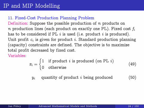
11. Fixed-Cost Production Planning ProblemDefinition: Suppose the possible production of n products onn production lines (each product on exactly one PL). Fixed cost fihas to be considered if PL i is used (i.e. product i is produced).Unit profit ci is given for product i . Standard production planning(capacity) constraints are defined. The objective is to maximizetotal profit decreased by fixed cost.Variables:
xi =
(1 if product i is produced (on PL i)0 otherwise
(49)
yi = quantity of product i being produced (50)
Jan Fábry Advanced Mathematical Models and Methods 24 / 150

IP and MIP Modelling
11. Fixed-Cost Production Planning ProblemModel:
maxnXi=1
ciyi �nXi=1
fixi (51)
(capacity constraints)nXi=1
aliyi � bl for l = 1; 2; : : : ;m (52)
yi �Mxi for i = 1; 2; : : : ;n (53)
xi 2 f0; 1g for i = 1; 2; : : : ;n (54)
yi 2 R+ for i = 1; 2; : : : ;n (55)
M = big number
Jan Fábry Advanced Mathematical Models and Methods 25 / 150
IP and MIP Modelling
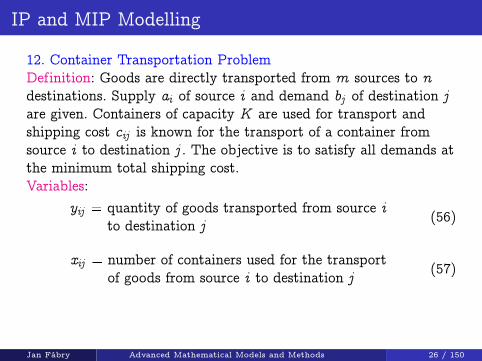
12. Container Transportation ProblemDefinition: Goods are directly transported from m sources to ndestinations. Supply ai of source i and demand bj of destination jare given. Containers of capacity K are used for transport andshipping cost cij is known for the transport of a container fromsource i to destination j . The objective is to satisfy all demands atthe minimum total shipping cost.Variables:
yij = quantity of goods transported from source ito destination j
(56)
xij = number of containers used for the transportof goods from source i to destination j
(57)
Jan Fábry Advanced Mathematical Models and Methods 26 / 150

IP and MIP Modelling
12. Container Transportation ProblemModel:
minmXi=1
nXj=1
cij xij (58)
nXj=1
yij � ai for i = 1; 2; : : : ;m (59)
mXi=1
yij = bj for j = 1; 2; : : : ;n (60)
yij � Kxij fori = 1; 2; : : : ;mj = 1; 2; : : : ;n
(61)
yij 2 R+ fori = 1; 2; : : : ;mj = 1; 2; : : : ;n
(62)
xij 2 Z+ fori = 1; 2; : : : ;mj = 1; 2; : : : ;n
(63)
Jan Fábry Advanced Mathematical Models and Methods 27 / 150
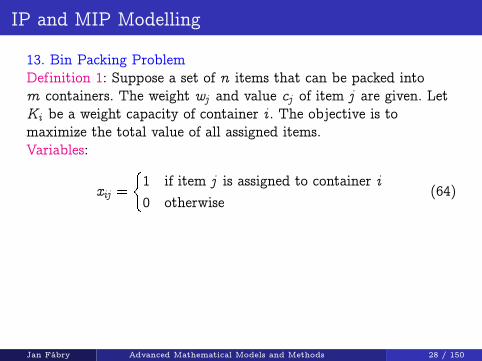
IP and MIP Modelling
13. Bin Packing ProblemDefinition 1: Suppose a set of n items that can be packed intom containers. The weight wj and value cj of item j are given. LetKi be a weight capacity of container i . The objective is tomaximize the total value of all assigned items.Variables:
xij =
(1 if item j is assigned to container i0 otherwise
(64)
Jan Fábry Advanced Mathematical Models and Methods 28 / 150

IP and MIP Modelling
13. Bin Packing ProblemModel:
maxmXi=1
nXj=1
cj xij (65)
mXi=1
xij � 1 for j = 1; 2; : : : ;n (66)
nXj=1
wj xij � Ki for i = 1; 2; : : : ;m (67)
xij 2 f0; 1g fori = 1; 2; : : : ;mj = 1; 2; : : : ;n
(68)
Jan Fábry Advanced Mathematical Models and Methods 29 / 150

IP and MIP Modelling
13. Bin Packing ProblemDefinition 2: Suppose a set of n types of items that have to betransported using m containers of identical weight capacity K . Letwj be a weight of item type j and rj be a number of them to betransported. The objective is to minimize a number of containersused to transport all items.Variables:
xi =
(1 if container i is used0 otherwise
(69)
yij = a number of items of type j beingtransported in container i
(70)
Jan Fábry Advanced Mathematical Models and Methods 30 / 150

IP and MIP Modelling
13. Bin Packing ProblemModel:
minmXi=1
xi (71)
mXi=1
yij = rj for j = 1; 2; : : : ;n (72)
nXj=1
wjyij � Kxi for i = 1; 2; : : : ;m (73)
xi 2 f0; 1g for i = 1; 2; : : : ;m (74)
yij 2 Z+ fori = 1; 2; : : : ;mj = 1; 2; : : : ;n
(75)
Jan Fábry Advanced Mathematical Models and Methods 31 / 150

Course Syllabus
1 Integer Programming Problem
2 IP and MIP Modelling
3 Graph ModellingFlow ProblemsRouting Problems
4 Formulations in Logical Variables
5 Polyhedral Theory
6 Solving Problems - Methods & AlgorithmsRelaxationExact MethodsComputational ComplexityHeuristics & Metaheuristics
Jan Fábry Advanced Mathematical Models and Methods 32 / 150
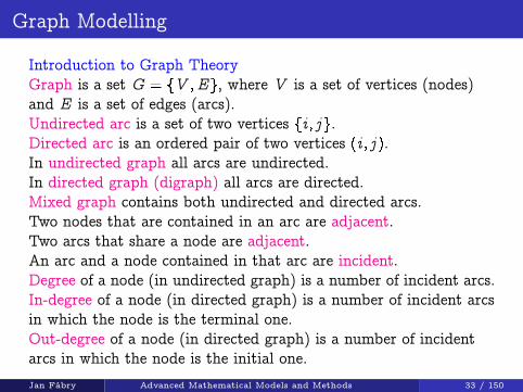
Graph Modelling
Introduction to Graph TheoryGraph is a set G = fV ;Eg, where V is a set of vertices (nodes)and E is a set of edges (arcs).Undirected arc is a set of two vertices fi ; j g.Directed arc is an ordered pair of two vertices (i ; j ).In undirected graph all arcs are undirected.In directed graph (digraph) all arcs are directed.Mixed graph contains both undirected and directed arcs.Two nodes that are contained in an arc are adjacent.Two arcs that share a node are adjacent.An arc and a node contained in that arc are incident.Degree of a node (in undirected graph) is a number of incident arcs.In-degree of a node (in directed graph) is a number of incident arcsin which the node is the terminal one.Out-degree of a node (in directed graph) is a number of incidentarcs in which the node is the initial one.
Jan Fábry Advanced Mathematical Models and Methods 33 / 150
Graph Modelling
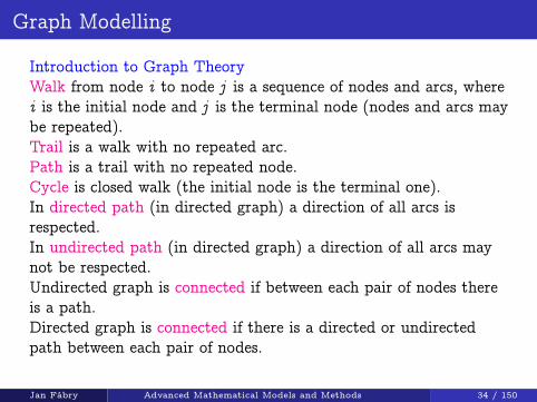
Introduction to Graph TheoryWalk from node i to node j is a sequence of nodes and arcs, wherei is the initial node and j is the terminal node (nodes and arcs maybe repeated).Trail is a walk with no repeated arc.Path is a trail with no repeated node.Cycle is closed walk (the initial node is the terminal one).In directed path (in directed graph) a direction of all arcs isrespected.In undirected path (in directed graph) a direction of all arcs maynot be respected.Undirected graph is connected if between each pair of nodes thereis a path.Directed graph is connected if there is a directed or undirectedpath between each pair of nodes.
Jan Fábry Advanced Mathematical Models and Methods 34 / 150

Graph Modelling
Introduction to Graph TheoryDirected graph is strongly connected if there is a directed pathbetween each pair of nodes.Undirected graph is complete if there is an arc between each pair ofnodes.Tree is a connected undirected graph with no cycles.Subgraph of graph G = fV ;Eg is a graph G 0 = fV 0;E 0g, whereV 0 � V and E 0 � E .Spanning tree of the graph G is a subgraph G 0, where V 0 = V andwhich is a tree.Valued graph has numbers associated with nodes or/and arcs.Hamiltonian cycle is a cycle that includes each node of the graphexactly once.Eulerian cycle includes each arc of the graph exactly once.Eulerian trail is a trail that includes each arc of the graph.Eulerian graph is a graph in which the Eulerian cycle can be found.
Jan Fábry Advanced Mathematical Models and Methods 35 / 150

Course Syllabus
1 Integer Programming Problem
2 IP and MIP Modelling
3 Graph ModellingFlow ProblemsRouting Problems
4 Formulations in Logical Variables
5 Polyhedral Theory
6 Solving Problems - Methods & AlgorithmsRelaxationExact MethodsComputational ComplexityHeuristics & Metaheuristics
Jan Fábry Advanced Mathematical Models and Methods 36 / 150

Flow Problems
1. Maximum Flow ProblemDefinition: Let G = fV ;Eg be a digraph with the flow capacity kijgiven for each arc (i ; j ). The objective is to identify the maximumamount of flow that can occur from source node s to sink node d .Variables: xij = flow from node i to node j (76)
F = total flow (77)
Model: max F (78)
Xj2V
(i ; j )2E
xij �Xj2V
(j ; i)2E
xji =
8>><>>:F for i = s0 for i 2 V n fs ; dg�F for i = d
(79)
xij � kij for (i ; j ) 2 E (80)
xij 2 R+ for (i ; j ) 2 E (81)
F 2 R+ (82)Jan Fábry Advanced Mathematical Models and Methods 37 / 150

Flow Problems
1. Maximum Flow ProblemAlternative approach to modelling: Adding a dummy backward arcfrom d to s with the capacity kds =M (big number).Variables:
xij = flow from node i to node j (83)
Model:max xds (84)X
j2V(i ; j )2E
xij �Xj2V
(j ; i)2E
xji = 0 for i 2 V (85)
xij � kij for (i ; j ) 2 E (86)
xij 2 R+ for (i ; j ) 2 E (87)
Jan Fábry Advanced Mathematical Models and Methods 38 / 150

Flow Problems
2. Minimum-Cost Flow ProblemDefinition: Let G = fV ;Eg be a digraph with the flow capacitykij and unit cost cij given for each arc (i ; j ). The objective is tosatisfy required total flow F0 (from source node s to sink node d)with the minimum total cost.Variables: xij = flow from node i to node j (88)
Model: minXi2V
Xj2V
(i ;j )2E
cij xij (89)
Xj2V
(i ; j )2E
xij �Xj2V
(j ; i)2E
xji =
8>><>>:F0 for i = s0 for i 2 V n fs ; dg�F0 for i = d
(90)
xij � kij for (i ; j ) 2 E (91)
xij 2 R+ for (i ; j ) 2 E (92)
Jan Fábry Advanced Mathematical Models and Methods 39 / 150
Flow Problems
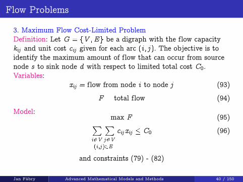
3. Maximum Flow Cost-Limited ProblemDefinition: Let G = fV ;Eg be a digraph with the flow capacitykij and unit cost cij given for each arc (i ; j ). The objective is toidentify the maximum amount of flow that can occur from sourcenode s to sink node d with respect to limited total cost C0.Variables:
xij = flow from node i to node j (93)
F = total flow (94)
Model:max F (95)X
i2V
Xj2V
(i ;j )2E
cij xij � C0 (96)
and constraints (79) - (82)
Jan Fábry Advanced Mathematical Models and Methods 40 / 150
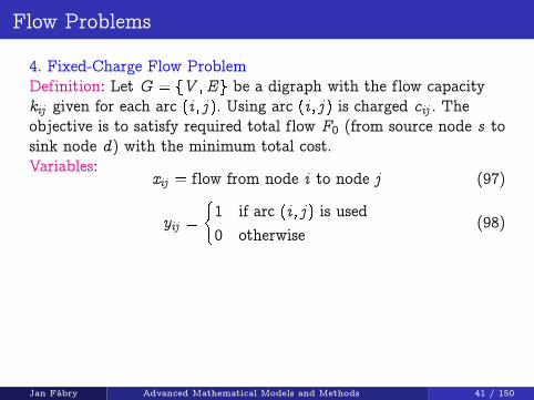
Flow Problems
4. Fixed-Charge Flow ProblemDefinition: Let G = fV ;Eg be a digraph with the flow capacitykij given for each arc (i ; j ). Using arc (i ; j ) is charged cij . Theobjective is to satisfy required total flow F0 (from source node s tosink node d) with the minimum total cost.Variables:
xij = flow from node i to node j (97)
yij =
(1 if arc (i ; j ) is used0 otherwise
(98)
Jan Fábry Advanced Mathematical Models and Methods 41 / 150
Flow Problems
4. Fixed-Charge Flow ProblemModel:
minXi2V
Xj2V
(i ;j )2E
cijyij (99)
Xj2V
(i ; j )2E
xij �Xj2V
(j ; i)2E
xji =
8>><>>:F0 for i = s0 for i 2 V n fs ; dg�F0 for i = d
(100)
xij � kijyij for (i ; j ) 2 E (101)
yij 2 f0; 1g for (i ; j ) 2 E (102)
Jan Fábry Advanced Mathematical Models and Methods 42 / 150
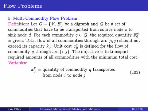
Flow Problems
5. Multi-Commodity Flow ProblemDefinition: Let G = fV ;Eg be a digraph and Q be a set ofcommodities that have to be transported from source node s tosink node d . For each commodity q 2 Q , the required quantity F q
0is given. Total flow of all commodities through arc (i ; j ) should notexceed its capacity kij . Unit cost c
qij is defined for the flow of
commodity q through arc (i ; j ). The objective is to transportrequired amounts of all commodities with the minimum total cost.Variables:
x qij = quantity of commodity q transportedfrom node i to node j
(103)
Jan Fábry Advanced Mathematical Models and Methods 43 / 150
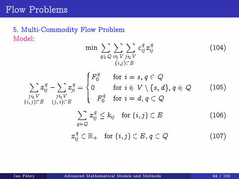
Flow Problems
5. Multi-Commodity Flow ProblemModel:
minXq2Q
Xi2V
Xj2V
(i ;j )2E
cqij xqij (104)
Xj2V
(i ; j )2E
x qij �Xj2V
(j ; i)2E
x qji =
8>><>>:F q0 for i = s ; q 2 Q
0 for i 2 V n fs ; dg; q 2 Q�F q
0 for i = d ; q 2 Q
(105)
Xq2Q
x qij � kij for (i ; j ) 2 E (106)
x qij 2 R+ for (i ; j ) 2 E ; q 2 Q (107)
Jan Fábry Advanced Mathematical Models and Methods 44 / 150

Flow Problems
6. Transshipment ProblemDefinition: Let G = fV ;Eg be a digraph with three sets of nodes:set of sources Vs , set of destinations Vd and set of transshipmentnodes Vt . Let ai > 0 be a supply of the product in source nodei 2 Vs and ai < 0 be a demand for the product in destinationi 2 Vd . For each transshipment node i 2 Vt it is valid ai = 0. Flowcapacity kij and unit cost cij are given for each arc (i ; j ). Demandin all destinations has to be satisfied without exceeding any supply.The objective is to minimize total flow cost. Suppose total demandis equal to total supply.Assumptions:
V = Vs[Vd[Vt and Vs\Vd\Vt = ; (108)Xi2Vs
ai +Xi2Vd
ai = 0 (109)
Jan Fábry Advanced Mathematical Models and Methods 45 / 150

Flow Problems
6. Transshipment ProblemVariables:
xij = flow from node i to node j (110)
Model:min
Xi2V
Xj2V
(i ;j )2E
cij xij (111)
Xj2V
(i ; j )2E
xij �Xj2V
(j ; i)2E
xji = ai for i 2 V (112)
xij � kij for (i ; j ) 2 E (113)
xij 2 R+ for (i ; j ) 2 E (114)
Jan Fábry Advanced Mathematical Models and Methods 46 / 150

Flow Problems
7. Minimal Spanning TreeDefinition: Let G = fV ;Eg be an undirected graph with cost cijgiven for each arc fi ; j g. The objective is to search a spanning treeof G minimizing total cost.Graph transformation: Set of undirected arcs E is transformed toset of directed arcs A in the following way:Each arc fi ; j g 2 E is replaced with directed arcs (i ; j ) 2 A and(j ; i) 2 A, cji = cij .Variables:
xij =
(1 if arc (i ; j ) is selected0 otherwise
(115)
yij = flow from node i to node j (116)
Jan Fábry Advanced Mathematical Models and Methods 47 / 150
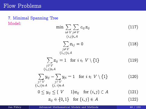
Flow Problems
7. Minimal Spanning TreeModel:
minXi2V
Xj2V
(i ;j )2A
cij xij (117)
Xj2V
(1; j )2A
x1j = 0 (118)
Xj2V
(i ; j )2A
xij = 1 for i 2 V n f1g (119)
Xj2V
(i ; j )2A
yij �Xj2V
(j ; i)2A
yji = 1 for i 2 V n f1g (120)
0 � yij � (jV j � 1)xij for (i ; j ) 2 A (121)
xij 2 f0; 1g for (i ; j ) 2 A (122)
Jan Fábry Advanced Mathematical Models and Methods 48 / 150

Flow Problems
8. Minimal Steiner TreeDefinition: Let G = fV ;Eg be a digraph, s 2 V be a source of thesignal (transmitter), D � V a set of users (receivers, destinations)and T � V a set of transfer stations. Using cables, users can beconnected to transmitter directly or through the transfer stations.Let cij be cost for connection (i ; j ) 2 E . The use of transfer stationi 2 T is charged fi . The objective is to connect all users to thesource with the minimal total cost.Variables:
zi =
(1 if node i is selected0 otherwise
(123)
xij =
(1 if arc (i ; j ) is selected0 otherwise
(124)
yij = flow from node i to node j (125)
Jan Fábry Advanced Mathematical Models and Methods 49 / 150

Flow Problems
8. Minimal Steiner TreeModel:
minXi2V
Xj2V
(i ;j )2E
cij xij +Xi2T
fizi (126)
zi = 1 for i 2 D (127)Xj2V
(i ; j )2E
xij = zi for i 2 V n fsg (128)
Xj2V
(i ; j )2E
yij �Xj2V
(j ; i)2E
yji = zi for i 2 V n fsg (129)
0 � yij � (jV j � 1)xij for (i ; j ) 2 E (130)
xij 2 f0; 1g for (i ; j ) 2 E (131)
zi 2 f0; 1g for i 2 T (132)
Jan Fábry Advanced Mathematical Models and Methods 50 / 150

Course Syllabus
1 Integer Programming Problem
2 IP and MIP Modelling
3 Graph ModellingFlow ProblemsRouting Problems
4 Formulations in Logical Variables
5 Polyhedral Theory
6 Solving Problems - Methods & AlgorithmsRelaxationExact MethodsComputational ComplexityHeuristics & Metaheuristics
Jan Fábry Advanced Mathematical Models and Methods 51 / 150

Routing Problems
Classification of ProblemsNetwork routing
I Node routingF Travelling Salesman Problem (TSP) - infinite capacity of
vehiclesF Vehicle Routing Problem (VRP) - limited capacity of vehicles
I Arc routingF Chinese Postman Problem (CPP)
Number of depots and vehiclesI One depot with one or multiple vehiclesI Multiple depots
Knowledge of customersI Static problems - all customers are known in advanceI Dynamic problems - advanced customers and on-line customers
ObjectiveI Total travelled distance (total cost) minimizationI Total travelled time minimizationI Minimizing the longest time of completing all routes
Jan Fábry Advanced Mathematical Models and Methods 52 / 150

Routing Problems
1. Travelling Salesman ProblemDefinition: Let G = fU ;Eg be a complete digraph with distancecij given for each arc (i ; j ) (matrix C is generally asymmetric). Letnode 1 be a depot and jU j = n . The objective is to determine theminimal Hamiltonian cycle.Variables:
xij =
8>><>>:1 if a vehicle travels directly
between nodes i and j0 otherwise
(133)
ui = dummy variable in sub-tours eliminating constraints (134)
Jan Fábry Advanced Mathematical Models and Methods 53 / 150

Routing Problems
1. Travelling Salesman ProblemModel (Miller, Tucker, Zemlin):
minnXi=1
nXj=1
cij xij (135)
nXj=1
xij = 1 for i = 1; 2; : : : ;n (136)
nXi=1
xij = 1 for j = 1; 2; : : : ;n (137)
ui + 1� (n � 1)(1� xij ) � uj fori = 1; 2; : : : ;nj = 2; 3; : : : ;n
(138)
xij 2 f0; 1g fori = 1; 2; : : : ;nj = 1; 2; : : : ;n
(139)
ui 2 R+ for i = 1; 2; : : : ;n (140)Jan Fábry Advanced Mathematical Models and Methods 54 / 150

Routing Problems
2. Travelling Salesman Problem with Time Windows (TSPTW)Definition: Let Asymmetric TSP be defined. Each node i has to bevisited within time interval hei ; li i. A vehicle spends given time Siat node i . Let dij be the traversal time between nodes i and j . Theobjective is to determine the minimal Hamiltonian cycle (in termsof distance) respecting all time windows.Variables:
xij =
8>><>>:1 if a vehicle travels directly
between nodes i and j0 otherwise
(141)
ti = time node i is visited (142)
Jan Fábry Advanced Mathematical Models and Methods 55 / 150
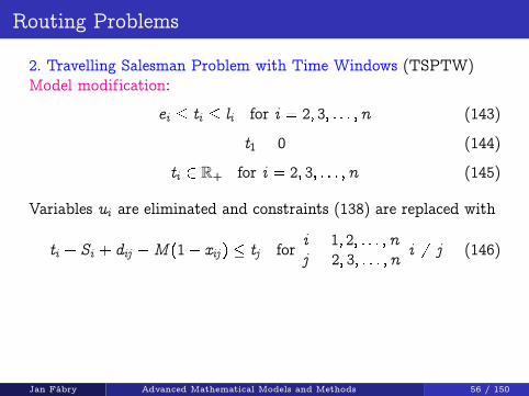
Routing Problems
2. Travelling Salesman Problem with Time Windows (TSPTW)Model modification:
ei � ti � li for i = 2; 3; : : : ;n (143)
t1 = 0 (144)
ti 2 R+ for i = 2; 3; : : : ;n (145)
Variables ui are eliminated and constraints (138) are replaced with
ti + Si + dij �M (1� xij ) � tj fori = 1; 2; : : : ;nj = 2; 3; : : : ;n
i 6= j (146)
Jan Fábry Advanced Mathematical Models and Methods 56 / 150

Routing Problems
3. Metric TSP (� - TSP)Triangle inequality:
cij � cik + ckj for i ; j ; k = 1; 2; : : : ;n ; i 6= j 6= k (147)
4. Euclidian TSP (Planar TSP)Euclidian distance:
cij =q(Xi �Xj )
2 + (Yi �Yj )2 for i ; j = 1; 2; : : : ;n ; i 6= j (148)
5. Open TSPInstead of minimal Hamiltonian cycle, minimal open path throughall nodes is being searched for (a tour is not finished at the depot):
we set ci1 = 0 for i = 2; 3; : : : ;n (149)
Jan Fábry Advanced Mathematical Models and Methods 57 / 150
Routing Problems
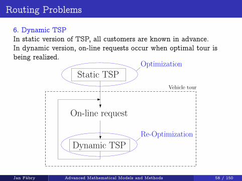
6. Dynamic TSPIn static version of TSP, all customers are known in advance.In dynamic version, on-line requests occur when optimal tour isbeing realized.
Static TSP
Dynamic TSP
On-line request
Re-Optimization
Optimization
Vehicle tour
Jan Fábry Advanced Mathematical Models and Methods 58 / 150

Routing Problems
7. Vehicle Routing ProblemDefinition: Let G = fU ;Eg be a complete digraph with distancecij given for each arc (i ; j ). Let node 1 be a depot, where onevehicle with capacity V is available. Let jU j = n . Each customer iis associated with request of size qi . The objective is to satisfy allcustomers’ requirements and to minimize total length of the routes.Variables:
xij =
8>><>>:1 if a vehicle travels directly
between nodes i and j0 otherwise
(150)
ui = dummy variable for the balance of load on the vehicle (151)
Assumptions: nXi=2
qi > V (152)
qi � V for i = 2; 3; : : : ;n (153)
Jan Fábry Advanced Mathematical Models and Methods 59 / 150

Routing Problems
7. Vehicle Routing ProblemModel:
minnXi=1
nXj=1
cij xij (154)nX
j=1
xij = 1 for i = 2; 3; : : : ;n (155)
nXi=1
xij = 1 for j = 2; 3; : : : ;n (156)
ui + qj �V (1� xij ) � uj fori = 1; 2; : : : ;nj = 2; 3; : : : ;n
(157)
ui � V for i = 2; 3; : : : ;n (158)
u1 = 0 (159)
xij 2 f0; 1g fori = 1; 2; : : : ;nj = 1; 2; : : : ;n
(160)
ui 2 R+ for i = 2; 3; : : : ;n (161)Jan Fábry Advanced Mathematical Models and Methods 60 / 150

Routing Problems
8. Heterogenous Fleet Vehicle Routing ProblemDefinition: Let VRP be defined with K types of vehicles availablein depot. For each type k its capacity Vk , available number pk andcost coefficient dk are given. The objective is to satisfy allcustomers’ requirements and to minimize total cost.Variables:
x kij =
8>><>>:1 if a vehicle of type k travels directly
between nodes i and j0 otherwise
(162)
ui = dummy variable for the balance of load on the vehicle (163)
Assumption: nXi=2
qi �KXk=1
pkVk (164)
Notation:V = max
k=1;2;:::;KVk (165)
Jan Fábry Advanced Mathematical Models and Methods 61 / 150

Routing Problems
8. Heterogenous Fleet Vehicle Routing ProblemModel:
minKXk=1
nXi=1
nXj=1
dkcij x kij (166)
KXk=1
nXj=1
x kij = 1 for i = 2; 3; : : : ;n (167)
nXi=1
x kij =nXi=1
x kji forj = 1; 2; : : : ;nk = 1; 2; : : : ;K
(168)
nXj=2
x k1j � pk for k = 1; 2; : : : ;K (169)
ui + qj �V (1� x kij ) � uj fori = 1; 2; : : : ;nj = 2; 3; : : : ;nk = 1; 2; : : : ;K
(170)
Jan Fábry Advanced Mathematical Models and Methods 62 / 150
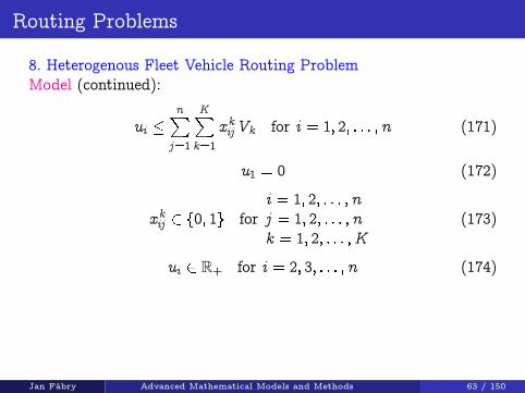
Routing Problems
8. Heterogenous Fleet Vehicle Routing ProblemModel (continued):
ui �nX
j=1
KXk=1
x kijVk for i = 1; 2; : : : ;n (171)
u1 = 0 (172)
x kij 2 f0; 1g fori = 1; 2; : : : ;nj = 1; 2; : : : ;nk = 1; 2; : : : ;K
(173)
ui 2 R+ for i = 2; 3; : : : ;n (174)
Jan Fábry Advanced Mathematical Models and Methods 63 / 150
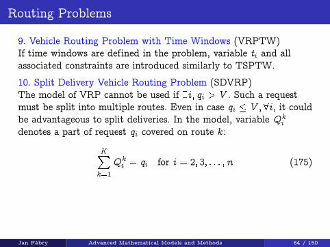
Routing Problems
9. Vehicle Routing Problem with Time Windows (VRPTW)If time windows are defined in the problem, variable ti and allassociated constraints are introduced similarly to TSPTW.
10. Split Delivery Vehicle Routing Problem (SDVRP)The model of VRP cannot be used if 9i ; qi > V . Such a requestmust be split into multiple routes. Even in case qi � V ;8i , it couldbe advantageous to split deliveries. In the model, variable Qk
idenotes a part of request qi covered on route k :
KXk=1
Qki = qi for i = 2; 3; : : : ;n (175)
Jan Fábry Advanced Mathematical Models and Methods 64 / 150

Routing Problems
11. Pickup and Delivery Problem (PDP)One-to-One PDP (Dial-a-Ride Problem, Messenger Problem)Each request originates at one location and is destined foranother location. Vehicle routes start and end at a commondepot.Many-to-Many PDPCommodity may be picked up at one of many locations andalso be delivered to one of many locations.One-to-Many-to-One PDPEach customer receives a delivery originating at a commondepot and sends a pickup quantity to the depot.
Jan Fábry Advanced Mathematical Models and Methods 65 / 150

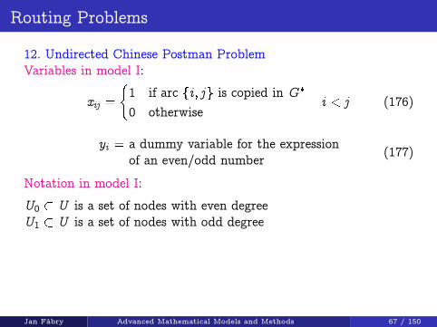
Routing Problems
12. Undirected Chinese Postman ProblemDefinition: Let G = fU ;Eg be an undirected and connected graph.Cost cij for each arc fi ; j g is given. The objective is to finda minimum cost tour passing through each arc at least once.
Theorem: An undirected graph G is Eulerian if and only if G isconnected and the degrees of all of its nodes are even.
If G is not Eulerian, we will construct a supergraph G� of G suchthat G� is Eulerian and includes an Eulerian tour that is shorterthan the Eulerian tour in any other supergraph of G .
Jan Fábry Advanced Mathematical Models and Methods 66 / 150
Routing Problems
12. Undirected Chinese Postman ProblemVariables in model I:
xij =
(1 if arc fi ; j g is copied in G�
0 otherwisei < j (176)
yi = a dummy variable for the expressionof an even/odd number
(177)
Notation in model I:
U0 � U is a set of nodes with even degreeU1 � U is a set of nodes with odd degree
Jan Fábry Advanced Mathematical Models and Methods 67 / 150
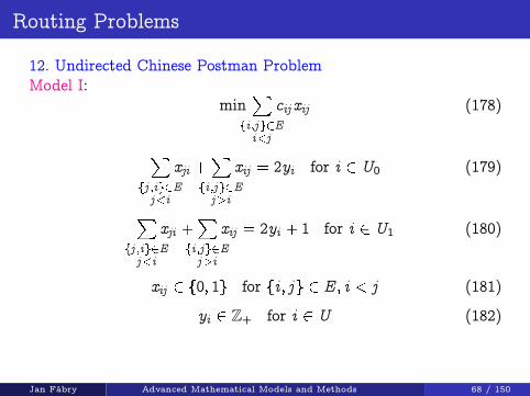
Routing Problems
12. Undirected Chinese Postman ProblemModel I:
minX
fi ;jg2Ei<j
cij xij (178)
Xfj ;ig2Ej<i
xji +X
fi ;jg2Ej>i
xij = 2yi for i 2 U0 (179)
Xfj ;ig2Ej<i
xji +X
fi ;jg2Ej>i
xij = 2yi + 1 for i 2 U1 (180)
xij 2 f0; 1g for fi ; j g 2 E ; i < j (181)
yi 2 Z+ for i 2 U (182)
Jan Fábry Advanced Mathematical Models and Methods 68 / 150

Routing Problems
12. Undirected Chinese Postman ProblemVariables in model II:
xij = a number of copies of arc fi ; j g in G� (183)
Model II:min
Xfi ;jg2E
cij xij (184)
xij + xji � 1 for fi ; j g; fj ; ig 2 E (185)Xfj ;ig2E
xji =X
fi ;jg2E
xij for i 2 U (186)
xij 2 Z+ for fi ; j g 2 E (187)
Jan Fábry Advanced Mathematical Models and Methods 69 / 150

Routing Problems
13. Directed Chinese Postman ProblemDefinition: Let G = fU ;Eg be a strongly connected digraph. Costcij for each arc (i ; j ) is given. The objective is to find a minimumcost tour passing through each arc at least once.
Theorem: An directed graph G is Eulerian if and only if G isstrongly connected and in-degree of each node is equal to itsout-degree.
If G is not Eulerian, we will construct a supergraph G� of G suchthat G� is Eulerian and includes an Eulerian tour that is shorterthan the Eulerian tour in any other supergraph of G .
Jan Fábry Advanced Mathematical Models and Methods 70 / 150

Routing Problems
13. Directed Chinese Postman ProblemNotation:
deg–i = in-degree of node ideg+i = out-degree of node iI = set of nodes i for which deg–i > deg+iJ = set of nodes j for which deg–j < deg+jai = deg–i � deg+i for i 2 Ibj = deg+j � deg–j for j 2 Jdij = the length of a shortest path from i 2 I to j 2 J
Variables:xij = a number of extra times each arc of the shortest
path from i to j has to be traversed(188)
Jan Fábry Advanced Mathematical Models and Methods 71 / 150

Routing Problems
13. Directed Chinese Postman ProblemModel:
minXi2I
Xj2J
dij xij (189)
Xj2J
xij = ai for i 2 I (190)
Xi2I
xij = bj for j 2 J (191)
xij 2 R+ fori 2 Ij 2 J
(192)
Jan Fábry Advanced Mathematical Models and Methods 72 / 150

Routing Problems
14. Mixed Chinese Postman Problem (street sweeping)CPP on mixed graph G = fU ;Eg is defined.
15. Rural Postman Problem (mail delivery)Let G = fU ;Eg be a connected graph with set R � E of requiredarcs that must be traversed at least once. The remaining arcs inE nR are optional and may be used in the optimal solution.
16. Capacitated Arc Routing Problem (garbage collection)Let G = fU ;Eg be a connected graph with requirement qij givenfor each arc fi ; j g (for each required arc in a rural version).Capacity of a vehicle covering requirements is limited. Multipletours have to be found without exceeding the vehicle capacity onany of them.
17. Hierarchical Postman Problem (snow plowing)Different priority levels are defined for arcs in the graph.
Jan Fábry Advanced Mathematical Models and Methods 73 / 150

Course Syllabus
1 Integer Programming Problem
2 IP and MIP Modelling
3 Graph ModellingFlow ProblemsRouting Problems
4 Formulations in Logical Variables
5 Polyhedral Theory
6 Solving Problems - Methods & AlgorithmsRelaxationExact MethodsComputational ComplexityHeuristics & Metaheuristics
Jan Fábry Advanced Mathematical Models and Methods 74 / 150

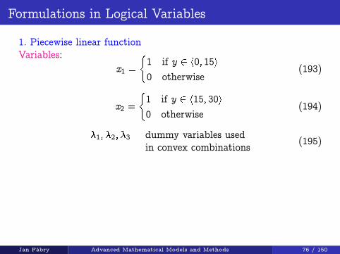
Formulations in Logical Variables
1. Piecewise linear functionDefinition: Let piecewise linear function f (y) be defined on a set ofintervals I1; I2; : : : ; Ir�1 denoted ha1; a2i; ha2; a3i; : : : ; har�1; ar i.For each interval bound ak , function value f (ak ) is given.Create a model of the function with the use of discrete variables.Example:
a1 = 0a2 = 15a3 = 30
f (a1) = 10f (a2) = 30f (a3) = 20
0 15 30
10
20
30
y
f (y)
Jan Fábry Advanced Mathematical Models and Methods 75 / 150
Formulations in Logical Variables
1. Piecewise linear functionVariables:
x1 =
(1 if y 2 h0; 15i0 otherwise
(193)
x2 =
(1 if y 2 h15; 30i0 otherwise
(194)
�1; �2; �3 = dummy variables usedin convex combinations
(195)
Jan Fábry Advanced Mathematical Models and Methods 76 / 150

Formulations in Logical Variables
1. Piecewise linear functionFormulation:
If y 2 h0; 15i then
y = 0�1 + 15�2 = a1�1 + a2�2f (y) = 10�1 + 30�2 = f (a1)�1 + f (a2)�2
)�1 + �2 = 1�1; �2 2 R+
(196)
If y 2 h15; 30i then
y = 15�2 + 30�3 = a2�2 + a3�3f (y) = 30�2 + 20�3 = f (a2)�2 + f (a3)�3
)�2 + �3 = 1�2; �3 2 R+
(197)
x1 = 0) �1 = 0x2 = 0) �3 = 0
) �1 � x1�3 � x2(�2 � x1 + x2)�
(198)
* The inequality is important in case of more than 2 intervals beingdefined (x1 = 0 ^ x2 = 0) �2 = 0):Jan Fábry Advanced Mathematical Models and Methods 77 / 150
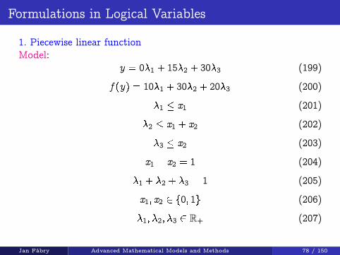
Formulations in Logical Variables
1. Piecewise linear functionModel:
y = 0�1 + 15�2 + 30�3 (199)
f (y) = 10�1 + 30�2 + 20�3 (200)
�1 � x1 (201)
�2 � x1 + x2 (202)
�3 � x2 (203)
x1 + x2 = 1 (204)
�1 + �2 + �3 = 1 (205)
x1; x2 2 f0; 1g (206)
�1; �2; �3 2 R+ (207)
Jan Fábry Advanced Mathematical Models and Methods 78 / 150

Formulations in Logical Variables
1. Piecewise linear functionVariables in general model:
xi =
(1 if y 2 Ii = hai ; ai+1i
0 otherwisefor i = 1; 2; : : : ; r � 1 (208)
�i = dummy variable usedin convex combinations
for i = 1; 2; : : : ; r (209)
General model:y =
rXi=1
ai�i (210)
f (y) =rX
i=1
f (ai )�i (211)
Jan Fábry Advanced Mathematical Models and Methods 79 / 150

Formulations in Logical Variables
1. Piecewise linear functionGeneral model (continued):
r�1Xi=1
xi = 1 (212)
rXi=1
�i = 1 (213)
�1 � x1 (214)
�r � xr�1 (215)
�i � xi�1 + xi for i = 2; 3; : : : ; r � 1 (216)
xi 2 f0; 1g for i = 1; 2; : : : ; r � 1 (217)
�i 2 R+ for i = 1; 2; : : : ; r (218)
Jan Fábry Advanced Mathematical Models and Methods 80 / 150

Formulations in Logical Variables
2. Nonconvex solution spaceExample: Let the following model be given. Use discrete variablesit could be solved as MIP model.
y1 + y2 � 40y1 � 20 or y2 � 10
y1; y2 2 R+
Variables:x1 =
(1 if y1 � 200 otherwise
(219)
x2 =
(1 if y2 � 100 otherwise
(220)
Jan Fábry Advanced Mathematical Models and Methods 81 / 150

Formulations in Logical Variables
2. Nonconvex solution spaceModel:
y1 + y2 � 40 (221)
y1 � 20x1 (222)
y2 � 10x2 (223)
x1 + x2 � 1 (224)
y1; y2 2 R+ (225)
x1; x2 2 f0; 1g (226)
Jan Fábry Advanced Mathematical Models and Methods 82 / 150

Formulations in Logical Variables
3. Disjunctive constraints (either-or constraints)Example: Three products can be produced on a machine either inthe sequence P1 ! P2 ! P3 or P3 ! P2 ! P1. Assume productionof Pi takes ti . Formulate the constraints for allowable production.Variables:
yi = starting production time of product Pi (227)
x =
(1 if sequence P1 ! P2 ! P3 is used0 if sequence P3 ! P2 ! P1 is used
(228)
Jan Fábry Advanced Mathematical Models and Methods 83 / 150

Formulations in Logical Variables
3. Disjunctive constraints (either-or constraints)Model:
y1 + t1 � y2 +M (1� x ) (229)
y2 + t2 � y3 +M (1� x ) (230)
y3 + t3 � y2 +Mx (231)
y2 + t2 � y1 +Mx (232)
yi 2 R+ for i = 1; 2; 3 (233)
x 2 f0; 1g (234)
Jan Fábry Advanced Mathematical Models and Methods 84 / 150

Formulations in Logical Variables
4. Disjunctive constraints (k out of m constraints must hold)Example: Suppose a model includes a set of m constraints. Letconstraint i be defined as aT
i y � bi . Assure exactly k of allconstraints must hold (k < m).Dummy variables:
xi =
(1 if constraint i is chosen0 otherwise
(235)
Constraints:
aTi y � bi +M (1� xi ) for i = 1; 2; : : : ;m (236)
mXi=1
xi = k (237)
Jan Fábry Advanced Mathematical Models and Methods 85 / 150
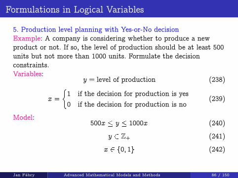
Formulations in Logical Variables
5. Production level planning with Yes-or-No decisionExample: A company is considering whether to produce a newproduct or not. If so, the level of production should be at least 500units but not more than 1000 units. Formulate the decisionconstraints.Variables:
y = level of production (238)
x =
(1 if the decision for production is yes0 if the decision for production is no
(239)
Model:500x � y � 1000x (240)
y 2 Z+ (241)
x 2 f0; 1g (242)
Jan Fábry Advanced Mathematical Models and Methods 86 / 150

Formulations in Logical Variables
6. Planning production on discrete levelsExample: A company decides to produce either 500 or 1000 or 2000units of certain product. Formulate the decision constraints.Variables:
y = level of production (243)
xi =
(1 if the production is set on i -th level0 otherwise
i = 1; 2; 3 (244)
Model:y = 500x1 + 1000x2 + 2000x3 (245)
x1 + x2 + x3 = 1 (246)
y 2 Z+ (247)
xi 2 f0; 1g for i = 1; 2; 3 (248)
Jan Fábry Advanced Mathematical Models and Methods 87 / 150
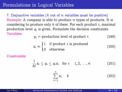
Formulations in Logical Variables
7. Disjunctive variables (k out of n variables must be positive)Example: A company is able to produce n types of products. It isconsidering to produce only k of them. For each product i , maximalproduction level qi is given. Formulate the decision constraints.Variables:
yi = production level of product i (249)
xi =
(1 if product i is produced0 otherwise
(250)
Constraints:1M
xi � yi � qixi for i = 1; 2; : : : ;n (251)
nXi=1
xi = k (252)
Jan Fábry Advanced Mathematical Models and Methods 88 / 150
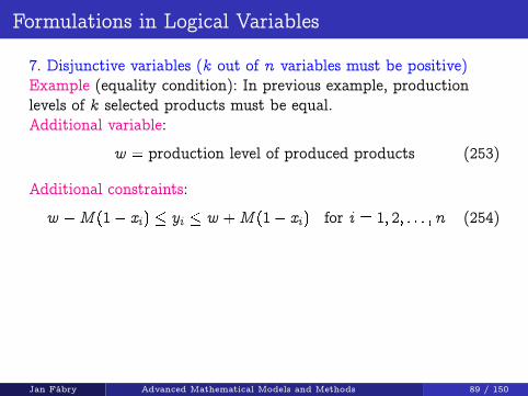
Formulations in Logical Variables
7. Disjunctive variables (k out of n variables must be positive)Example (equality condition): In previous example, productionlevels of k selected products must be equal.Additional variable:
w = production level of produced products (253)
Additional constraints:
w �M (1� xi ) � yi � w +M (1� xi ) for i = 1; 2; : : : ;n (254)
Jan Fábry Advanced Mathematical Models and Methods 89 / 150
Formulations in Logical Variables
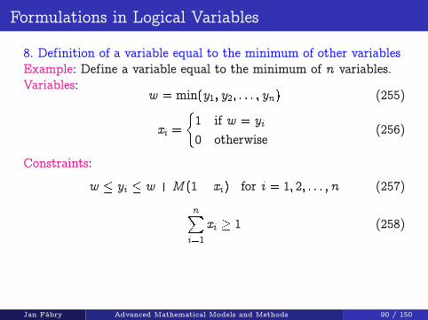
8. Definition of a variable equal to the minimum of other variablesExample: Define a variable equal to the minimum of n variables.Variables:
w = min(y1; y2; : : : ; yn) (255)
xi =
(1 if w = yi0 otherwise
(256)
Constraints:
w � yi � w +M (1� xi ) for i = 1; 2; : : : ;n (257)
nXi=1
xi � 1 (258)
Jan Fábry Advanced Mathematical Models and Methods 90 / 150

Formulations in Logical Variables
9. Simplifying Product of Binary VariablesExample: Simplify the maximization objective function x1x2x3(all variables are binary) to use a linear model (MIP model).Dummy variable:
w = x1x2x3 (259)
Model:max w (260)
x1 + x2 + x3 � 2 � w (261)
w � xi for i = 1; 2; 3 (262)
xi 2 f0; 1g for i = 1; 2; 3 (263)
w 2 R+ (264)
Jan Fábry Advanced Mathematical Models and Methods 91 / 150
Course Syllabus
1 Integer Programming Problem
2 IP and MIP Modelling
3 Graph ModellingFlow ProblemsRouting Problems
4 Formulations in Logical Variables
5 Polyhedral Theory
6 Solving Problems - Methods & AlgorithmsRelaxationExact MethodsComputational ComplexityHeuristics & Metaheuristics
Jan Fábry Advanced Mathematical Models and Methods 92 / 150
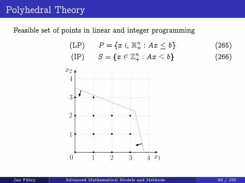
Polyhedral Theory
Feasible set of points in linear and integer programming
(LP) P = fx 2 Rn+ : Ax � bg (265)
(IP) S = fx 2 Zn+ : Ax � bg (266)
0 1 x1
x2
2 3
1
2
3
4
4
Jan Fábry Advanced Mathematical Models and Methods 93 / 150
Polyhedral Theory
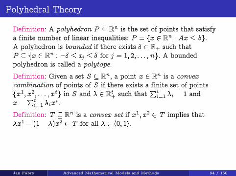
Definition: A polyhedron P � Rn is the set of points that satisfya finite number of linear inequalities: P = fx 2 Rn : Ax � bg.A polyhedron is bounded if there exists � 2 R+ such thatP � fx 2 Rn : �� � xj � � for j = 1; 2; : : : ;ng. A boundedpolyhedron is called a polytope.
Definition: Given a set S � Rn , a point x 2 Rn is a convexcombination of points of S if there exists a finite set of pointsfx 1; x 2; : : : ; x tg in S and � 2 Rt
+ such thatPt
i=1 �i = 1 andx =
Pti=1 �ix
i .
Definition: T � Rn is a convex set if x 1; x 2 2 T implies that�x 1 + (1� �)x 2 2 T for all � 2 h0; 1i.
Jan Fábry Advanced Mathematical Models and Methods 94 / 150

Polyhedral Theory
Definition: A convex hull of S , denoted by conv(S), is the set ofall points that are convex combinations of points in S .
0 1 x1
x2
2 3
1
2
3
4
4
S � conv(S) � P
Jan Fábry Advanced Mathematical Models and Methods 95 / 150

Polyhedral Theory
Definition: The inequality �Tx � �0 is called a valid inequality forS if it is satisfied by all points in S .
0 1 x1
x2
2 3
1
2
3
4
4
π Tx ≤ π0
Jan Fábry Advanced Mathematical Models and Methods 96 / 150

Polyhedral Theory
Definition: If �Tx � �0 is a valid inequality for S and 9x 0 2 S suchthat �Tx 0 = �0 we say that the inequality supports S . The setF = fx 2 conv(S) : �Tx = �0g is called a face of conv(S). We saythat the inequality �Tx � �0 represents F .
0 1 x1
x2
2 3
1
2
3
4
4
π Tx ≤ π0
F
Jan Fábry Advanced Mathematical Models and Methods 97 / 150

Polyhedral Theory
Definition: A face F of conv(S) is called a facet of conv(S) ifdim F = dim conv(S)� 1.
0 1 x1
x2
2 3
1
2
3
4
4
π Tx ≤ π
0F
Jan Fábry Advanced Mathematical Models and Methods 98 / 150

Polyhedral Theory
Definition: The valid inequalities �Tx � �0 and Tx � 0 are saidto be equivalent if = �� and 0 = ��0 for some � > 0.
Definition: Let �Tx � �0 and Tx � 0 be two valid inequalitiesfor conv(S) that are not equivalent. If there exists � > 0 such that � �� and 0 � ��0 then we say that Tx � 0 dominates or isstronger than �Tx � �0. We can also say that �Tx � �0 isdominated or is weaker than Tx � 0.
Observe that if Tx � 0 dominates �Tx � �0 thenfx 2 Rn
+ : Tx � 0g � fx 2 Rn+ : �Tx � �0g.
Definition: A maximal valid inequality is one that is notdominated by any other valid inequality.
Jan Fábry Advanced Mathematical Models and Methods 99 / 150

Polyhedral Theory
Any maximal valid inequality for S defines a nonempty face ofconv(S), and the set of maximal valid inequalities contains all ofthe facet-defining inequalities for conv(S).
0 1 x1
x2
2 3
1
2
3
4
4valid inequalitymaximal valid inequality
0 1 x1
x2
2 3
1
2
3
4
4valid
inequali
ty
maximal valid inequality
Jan Fábry Advanced Mathematical Models and Methods 100 / 150
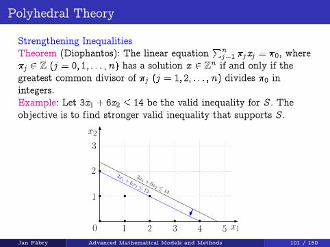
Polyhedral Theory
Strengthening InequalitiesTheorem (Diophantos): The linear equation
Pnj=1 �j xj = �0, where
�j 2 Z (j = 0; 1; : : : ;n) has a solution x 2 Zn if and only if thegreatest common divisor of �j (j = 1; 2; : : : ;n) divides �0 inintegers.Example: Let 3x1 + 6x2 � 14 be the valid inequality for S . Theobjective is to find stronger valid inequality that supports S .
0 1 x1
x2
2 3
1
2
3
4
3x1 + 6x
2 ≤ 14
5
3x1 + 6x
2 ≤ 12
Jan Fábry Advanced Mathematical Models and Methods 101 / 150

Polyhedral Theory
Strengthening Inequalities - LiftingDefinition: Let the inequality
Pnj=1 �j xj � �0 be given, where
�j 2 R+ (j = 0; 1; : : : ;n) and x 2 Bn . If for some �k > 0 theinequality
Pnj=1 �j xj +�kxk � �0 is valid, then it is said to have
been lifted from the original inequality with respect to xk .Algorithm:Repeat for k = 1; 2; : : : ;n :
1 Set xk = 1 and denote �k = maxxk2B
Pnj=1 �j xj � �0
2 Set �k = �0 � �k
3 Replace �k by �k +�k
4 The inequalityPn
j=1 �j xj � �0 is lifted with respect tovariable xk
The inequalityPn
j=1 �j xj � �0 is lifted with respect to all variables.
Jan Fábry Advanced Mathematical Models and Methods 102 / 150

Polyhedral Theory
Strengthening Inequalities - LiftingExample: Lift the inequality 4x1 + 5x2 + 6x3 + 8x4 � 13, wherexj 2 B (j = 1; 2; 3; 4).
x1 = 1! �1 = 12! �1 = 1! �1 = 5! 5x1+5x2+6x3+8x4 � 13
x2 = 1! �2 = 13! �2 = 0! �2 = 5! 5x1+5x2+6x3+8x4 � 13
x3 = 1! �3 = 11! �3 = 2! �3 = 8! 5x1+5x2+8x3+8x4 � 13
x4 = 1! �4 = 13! �4 = 0! �4 = 8! 5x1+5x2+8x3+8x4 � 13
Jan Fábry Advanced Mathematical Models and Methods 103 / 150

Polyhedral Theory
Strengthening Inequalities - Variable fixingExample: Let 2x1 + 3x2 + 4x3 � 15x4 � 2 with xj 2 B (j = 1; 2; 3; 4).If x4 = 1 the inequality cannot be satisfied ! feasible solutionsexist if variable is fixed x4 = 0.
Example: Let 20x1 + 5x2 + 1x3 � 8x4 � 7 with xj 2 B (j = 1; 2; 3; 4).Fixing x1 = 1.
Example: Let x1 + x2 + 3x3 = 4 with xj 2 B (j = 1; 2; 3).Because x3 = 0 is impossible, variable is fixed x3 = 1. Then, theequation is reduced to x1 + x2 = 1.
Jan Fábry Advanced Mathematical Models and Methods 104 / 150

Polyhedral Theory
Strengthening Inequalities - Gomory cutLet S = fx 2 Zn
+ : �Tx = �0g, where �j 2 R (j = 0; 1; : : : ;n). Letus select some d 2 N, then each �j is possible to express as
�j = �jd + �0j ; (267)
where �j =
��j
d
�and �0j = �j mod d . Thus �j 2 Z and �0j 2 h0; d).
Then, the equation nXj=1
�j xj = �0 (268)
can be written asnX
j=1
(�jd + �0j )xj = �0d + �00 (269)
ord(
nXj=1
�j xj � �0) = �00 �nX
j=1
�0j xj : (270)
Jan Fábry Advanced Mathematical Models and Methods 105 / 150

Polyhedral Theory
Strengthening Inequalities - Gomory cutBecause on left-hand side value in (270) is the integer multiple ofd , right-hand side must be also integer value. Due to �00 2 h0; d)and
Pnj=1 �
0j xj � 0, right-hand side value cannot be positive
multiple of d , i.e. it must be non-positive. Hence, left-hand sidevalue must be non-positive as well.
Fractional Gomory cut:
�00 �nX
j=1
�0j xj � 0 !nX
j=1
�0j xj � �00 (271)
All-integer Gomory cut:nX
j=1
�j xj � �0 � 0 !nX
j=1
�j xj � �0 (272)
Jan Fábry Advanced Mathematical Models and Methods 106 / 150
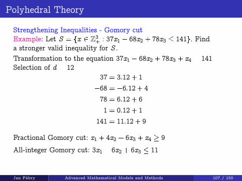
Polyhedral Theory
Strengthening Inequalities - Gomory cutExample: Let S = fx 2 Z3
+ : 37x1 � 68x2 + 78x3 � 141g. Finda stronger valid inequality for S .Transformation to the equation 37x1 � 68x2 + 78x3 + x4 = 141Selection of d = 12
37 = 3:12+ 1�68 = �6:12+ 478 = 6:12+ 61 = 0:12+ 1
141 = 11:12+ 9
Fractional Gomory cut: x1 + 4x2 + 6x3 + x4 � 9
All-integer Gomory cut: 3x1 � 6x2 + 6x3 � 11
Jan Fábry Advanced Mathematical Models and Methods 107 / 150

Course Syllabus
1 Integer Programming Problem
2 IP and MIP Modelling
3 Graph ModellingFlow ProblemsRouting Problems
4 Formulations in Logical Variables
5 Polyhedral Theory
6 Solving Problems - Methods & AlgorithmsRelaxationExact MethodsComputational ComplexityHeuristics & Metaheuristics
Jan Fábry Advanced Mathematical Models and Methods 108 / 150

Solving Problems - Methods & Algorithms
UnimodularityDefinition: A square, integer matrix A is called unimodular if itsdeterminant det(A) = �1. An integer matrix A is called totallyunimodular if every square, nonsingular submatrix of A isunimodular.Observation: If matrix A is totally unimodular, aij 2 f+1;�1; 0gfor all i ; j .Theorem (sufficient condition): A matrix A is totally unimodular if
aij 2 f+1;�1; 0g for all i ; jeach column contains at most two nonzero coefficientsthe rows of A can be partitioned into two sets such that
I if a column has two coefficients of the same sign, their rows arein different sets
I if a column has two coefficients of different signs, their rows arein the same set
Jan Fábry Advanced Mathematical Models and Methods 109 / 150

Solving Problems - Methods & Algorithms
UnimodularityLet the following linear programming problem with integral dataA; b be given:
zLP = maxfcTx : Ax � b; x 2 Rn+g: (273)
A vector of basic variables can be expressed as
xB = B�1b =Badj
det(B)b; (274)
where B is basis, B�1 its inverse and Badj is the adjoint matrix ofB (the transpose of the cofactor matrix of B).Observation: If the optimal basis B is unimodular, then theoptimum solution is integral.Proposition: If matrix A is totally unimodular, then the optimumsolution is integral.Examples: transportation problem, flow problem, ...
Jan Fábry Advanced Mathematical Models and Methods 110 / 150

Course Syllabus
1 Integer Programming Problem
2 IP and MIP Modelling
3 Graph ModellingFlow ProblemsRouting Problems
4 Formulations in Logical Variables
5 Polyhedral Theory
6 Solving Problems - Methods & AlgorithmsRelaxationExact MethodsComputational ComplexityHeuristics & Metaheuristics
Jan Fábry Advanced Mathematical Models and Methods 111 / 150
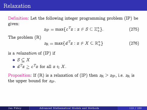
Relaxation
Definition: Let the following integer programming problem (IP) begiven:
zIP = maxfcTx : x 2 S � Zn+g: (275)
The problem (R)zR = maxfdTx : x 2 X � Rn
+g (276)
is a relaxation of (IP) ifS � XdTx � cTx for all x 2 X .
Proposition: If (R) is a relaxation of (IP) then zR � zIP, i.e. zR isthe upper bound for zIP.
Jan Fábry Advanced Mathematical Models and Methods 112 / 150

Relaxation
Linear Programming RelaxationDefinition: Let the following integer programming problem (IP) begiven:
zIP = maxfcTx : Ax � b; x 2 Zn+g: (277)
The problem (LP)
zLP = maxfcTx : Ax � b; x 2 Rn+g (278)
is a linear programming relaxation of (IP).
In case of binary integer programming problem (BIP)
zBIP = maxfcTx : Ax � b; x 2 Bng;B = f0; 1g (279)
a linear programming relaxation is defined as
zLP = maxfcTx : Ax � b; 0 � xj � 1; j = 1; 2; : : : ;ng: (280)
Jan Fábry Advanced Mathematical Models and Methods 113 / 150

Relaxation
Linear Programming RelaxationDefinition: The absolute integrality gap is defined as the difference
Gap = zLP � zIP (281)
and for zIP 6= 0, the relative integrality gap is defined as
Gap% =zLP � zIPjzIPj
100%: (282)
Linear programming relaxation can be also written as
zLP = maxfcTx : x 2 Qg; (283)
where S = fx : Ax � b; x 2 Zn+g � conv(S) � Q .
Jan Fábry Advanced Mathematical Models and Methods 114 / 150

Relaxation
Lagrangian RelaxationDefinition: Let the following integer programming problem (IP) begiven: zIP = maxfcTx : Ax � b; x 2 Zn
+g: (284)
The problem can be rewritten aszIP = maxfcTx : A1x � b1;A2x � b2; x 2 Zn
+g; (285)
where A =
A1
A2
!; b =
b1
b2
!.
A1x � b1 are m1 “complicating constraints” andA2x � b2 are m2 “nice constraints”.
Now for any � 2 Rm1+ , the problem (LR(�))
zLR(�) = maxfcTx + �T(b1 �A1x ) : A2x � b2; x 2 Zn+g (286)
is called the Lagrangian relaxation of (IP) with respect toA1x � b1.Jan Fábry Advanced Mathematical Models and Methods 115 / 150

Relaxation
Lagrangian RelaxationProposition: LR(�) is a relaxation of (IP) for all � � 0,i.e. zLR(�) � zIP for all � � 0.
Definition: The least upper bound available from the infinitefamily of relaxations f(LR(�)g��0 is zLR(��), where �� is anoptimal solution to the problem (LD)
zLD = min��0
zLR(�): (287)
Problem (LD) is called the Lagrangian dual of (IP) with respectto the constraints A1x � b1.
Jan Fábry Advanced Mathematical Models and Methods 116 / 150

Course Syllabus
1 Integer Programming Problem
2 IP and MIP Modelling
3 Graph ModellingFlow ProblemsRouting Problems
4 Formulations in Logical Variables
5 Polyhedral Theory
6 Solving Problems - Methods & AlgorithmsRelaxationExact MethodsComputational ComplexityHeuristics & Metaheuristics
Jan Fábry Advanced Mathematical Models and Methods 117 / 150
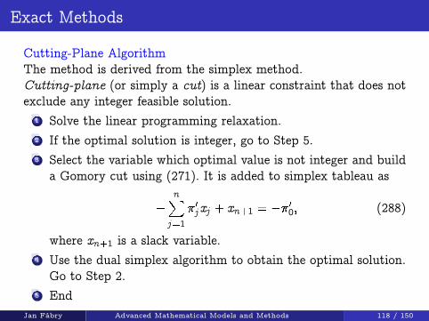
Exact Methods
Cutting-Plane AlgorithmThe method is derived from the simplex method.Cutting-plane (or simply a cut) is a linear constraint that does notexclude any integer feasible solution.
1 Solve the linear programming relaxation.2 If the optimal solution is integer, go to Step 5.3 Select the variable which optimal value is not integer and build
a Gomory cut using (271). It is added to simplex tableau as
�nX
j=1
�0j xj + xn+1 = ��00; (288)
where xn+1 is a slack variable.4 Use the dual simplex algorithm to obtain the optimal solution.
Go to Step 2.5 End
Jan Fábry Advanced Mathematical Models and Methods 118 / 150

Exact Methods
Branch and Bound AlgorithmIt is an enumerative algorithm.Proposition: Let the problem zIP = maxfcTx : x 2 Sg be given. LetS = S1[S2[ : : :[SK be a decomposition of S into smaller sets,and let z k = maxfcTx : x 2 Skg for k = 1; 2; : : : ;K . ThenzIP = maxk z k .Notation:M is a sequence of problems to be solved in particular branches ofan enumeration tree,x � is the best found integer solution,z � = cTx � is the best objective value.Algorithm:
1 Initial settingsM = (LP);LP is a linear programming relaxation,x � is not defined,z � = �1.
Jan Fábry Advanced Mathematical Models and Methods 119 / 150

Exact Methods
Branch and Bound Algorithm2 Selection of the problem to be solved
If M = () then go to Step 5else select the last problem in the sequence M .
3 Solution of selected problem(a) If no feasible solution exists then remove the problem from M
and go to Step 2.(b) If the optimal solution x 0 is found with the objective value z 0
then(b1) if z 0 � z � then remove the problem from M and go to Step 2,(b2) if z 0
> z � and x 0 is integer then set x � = x 0; z � = z 0, remove
the problem from M and go to Step 2,(b3) if z 0
> z � and x 0 is not integer then go to Step 4.
Jan Fábry Advanced Mathematical Models and Methods 120 / 150

Exact Methods
Branch and Bound Algorithm4 Branching
Select the variable xk the optimal value of which is not integer.Copy the last solving problem and add it to the end of thesequence M together with the constraint
xk � bx 0k c: (289)
Add the constraint
xk � bx 0k c+ 1 (290)
to the last but one problem in M .Go to Step 2.
5 EndPrint the optimum integer solution x � and the optimumobjective value z �.
Jan Fábry Advanced Mathematical Models and Methods 121 / 150

Exact Methods
Branch and Bound AlgorithmProposition: The enumeration tree can be pruned at the node ifany one of the following three conditions holds:
problem is infeasible,optimal solution x 0 is integer,it is valid z 0 � z �.
In case of binary enumeration tree (if n binary variables are given),n is a maximal depth of the tree and 2n is a maximal number ofleaves of the tree.
Jan Fábry Advanced Mathematical Models and Methods 122 / 150
Exact Methods
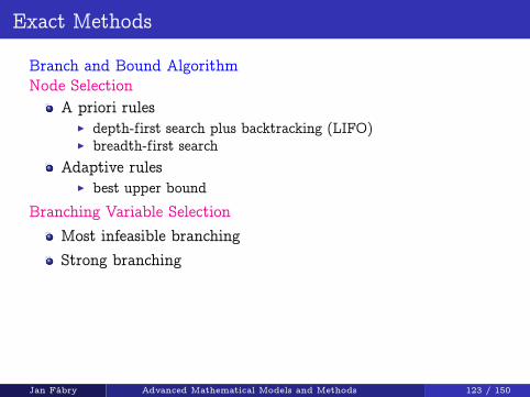
Branch and Bound AlgorithmNode Selection
A priori rulesI depth-first search plus backtracking (LIFO)I breadth-first search
Adaptive rulesI best upper bound
Branching Variable SelectionMost infeasible branchingStrong branching
Jan Fábry Advanced Mathematical Models and Methods 123 / 150
Exact Methods
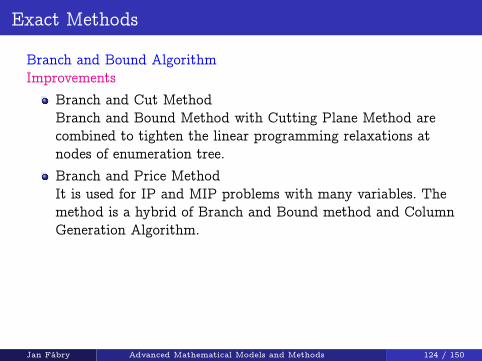
Branch and Bound AlgorithmImprovements
Branch and Cut MethodBranch and Bound Method with Cutting Plane Method arecombined to tighten the linear programming relaxations atnodes of enumeration tree.Branch and Price MethodIt is used for IP and MIP problems with many variables. Themethod is a hybrid of Branch and Bound method and ColumnGeneration Algorithm.
Jan Fábry Advanced Mathematical Models and Methods 124 / 150
Course Syllabus
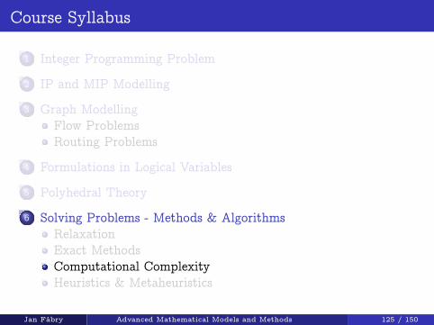
1 Integer Programming Problem
2 IP and MIP Modelling
3 Graph ModellingFlow ProblemsRouting Problems
4 Formulations in Logical Variables
5 Polyhedral Theory
6 Solving Problems - Methods & AlgorithmsRelaxationExact MethodsComputational ComplexityHeuristics & Metaheuristics
Jan Fábry Advanced Mathematical Models and Methods 125 / 150

Computational Complexity
Complexity of AlgorithmsThe size of an instance:
linear programmingm : : :number of constraintsn : : :number of variablesgraph modellingjU j : : :number of nodesjE j : : :number of arcs
Computational complexity of the algorithm is the function of thesize of an instance that the algorithm solves, e.g. f (n).
Jan Fábry Advanced Mathematical Models and Methods 126 / 150

Computational Complexity
Complexity of AlgorithmsLet elementary computer operation take 1 ns. The following tableshows the growth of computational time for various functionsdepending on a size of an instance.
f (n)n (size of instance)
10 20 50 100 1000n 10 ns 20 ns 50 ns 100 ns 1µs
n logn 10 ns 26 ns 85 ns 200 ns 3µsn2 100 ns 400 ns 2:5µs 10µs 1msn3 1µs 8µs 125µs 1ms 1 s2n 1µs 1ms 13 days 1013 years -3n 59µs 4 s 107 years - -n ! 4ms 77 years - - -
Jan Fábry Advanced Mathematical Models and Methods 127 / 150

Computational Complexity
Complexity of AlgorithmsWe are interested in the asymptotic rate of growth of thecomplexity of the algorithm.Definition: Let f (n); g(n) be functions from the positive integersto the positive reals.
We write f (n) = O(g(n)) if there exists a constant c > 0 suchthat, for large enough n ; f (n) � cg(n) (the big O notation).We write f (n) = (g(n)) if there exists a constant c > 0 suchthat, for large enough n ; f (n) � cg(n) (the big omeganotation).We write f (n) = �(g(n)) if there exist constants c; c0 > 0such that, for large enough n ; cg(n) � f (n) � c0g(n) (the bigtheta notation).
Polynomial algorithms: n ;n2;n3; logn ;n lognNon-polynomial algorithms: 2n ; en ;n !
Jan Fábry Advanced Mathematical Models and Methods 128 / 150

Computational Complexity
Complexity ClassesClass PIt is a class of decision problems that can be solved in polynomialtime. The decision problem of size n is in P if there exists thealgorithm with f (n) = O(np) fore some fixed p.Class POIt is a class of optimization problems that can be solved inpolynomial time. The optimization problem of size n is in PO ifthere exists the algorithm with f (n) = O(np) fore some fixed p.
Some problems solvable in polynomial time.Minimal spanning tree.Shortest path problem.Maximal flow problem.Assignment problem.Linear programming problem.
Jan Fábry Advanced Mathematical Models and Methods 129 / 150
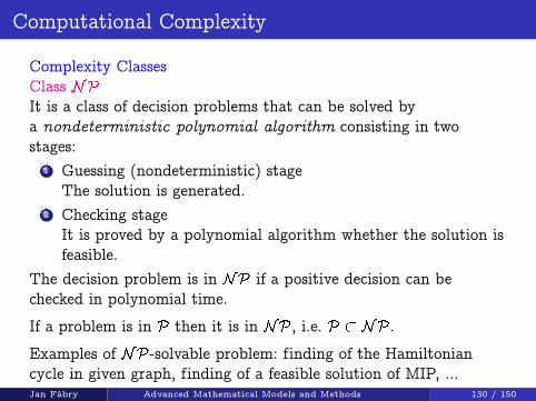
Computational Complexity
Complexity ClassesClass NPIt is a class of decision problems that can be solved bya nondeterministic polynomial algorithm consisting in twostages:
1 Guessing (nondeterministic) stageThe solution is generated.
2 Checking stageIt is proved by a polynomial algorithm whether the solution isfeasible.
The decision problem is in NP if a positive decision can bechecked in polynomial time.
If a problem is in P then it is in NP, i.e. P � NP.
Examples of NP-solvable problem: finding of the Hamiltoniancycle in given graph, finding of a feasible solution of MIP, ...Jan Fábry Advanced Mathematical Models and Methods 130 / 150

Computational Complexity
Complexity ClassesClass NPOThe optimization problem is in NPO if its decision version is inNP.
If a problem is in PO then it is in NPO, i.e. PO � NPO.
Definition: Decision problem A is polynomially reducible todecision problem B if there exists a polynomial functiontransforming definition of problem A to definition of problem Bsuch that from the solution of B , it is possible to derive thesolution of A.
If decision problem A is reducible to decision problem B then, ifwe have the algorithm to solve B , it can be used to solve A.
Decision problem A is a special instance of decision problem B ,i.e. B is more general and, therefore, more difficult.
Jan Fábry Advanced Mathematical Models and Methods 131 / 150

Computational Complexity
Complexity ClassesProposition: If A is polynomially reducible to B and B 2 P,then A 2 P.Proposition: If A is polynomially reducible to B and B 2 NP,then A 2 NP.
Class NPCDecision problem A 2 NP is said to be NP-complete if allproblems in NP can be polynomially reduced to A.
Proposition: If A 2 NPC is polynomially reducible to B 2 NP,then B 2 NPC.Corollary: In order to prove that a problem is NP-complete, wemust show:
that the problem is in NP andthat any known NP-complete problem is reducible to theproblem.
Jan Fábry Advanced Mathematical Models and Methods 132 / 150

Computational Complexity
Complexity ClassesProposition: If P \NPC 6= ; then P = NP.Corollary: If there is a polynomial algorithm to solve anyNP-complete problem then using the reducibility we will be ableto solve all problems in NP in polynomial time.
Examples of NP-complete problems (some of them are binaryversions of optimization problems):
Binary programming feasibility problem.Set partitioning feasibility problem.Knapsack lower-bound feasibility problem.Finding of Hamiltonian cycle.Travelling salesman upper-bound feasibility problem.Quadratic assignment upper-bound feasibility problem.Partition problem.
Jan Fábry Advanced Mathematical Models and Methods 133 / 150

Computational Complexity
Complexity ClassesClass NPHAn optimization problem is NP-hard if its decision version is inNPC.
Examples of NP-hard problems:IP problem.Knapsack problem.TSP.Minimal Steiner tree.Quadratic assignment problem.Container transportation problem.
Jan Fábry Advanced Mathematical Models and Methods 134 / 150

Course Syllabus
1 Integer Programming Problem
2 IP and MIP Modelling
3 Graph ModellingFlow ProblemsRouting Problems
4 Formulations in Logical Variables
5 Polyhedral Theory
6 Solving Problems - Methods & AlgorithmsRelaxationExact MethodsComputational ComplexityHeuristics & Metaheuristics
Jan Fábry Advanced Mathematical Models and Methods 135 / 150
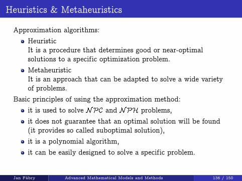
Heuristics & Metaheuristics
Approximation algorithms:HeuristicIt is a procedure that determines good or near-optimalsolutions to a specific optimization problem.MetaheuristicIt is an approach that can be adapted to solve a wide varietyof problems.
Basic principles of using the approximation method:it is used to solve NPC and NPH problems,it does not guarantee that an optimal solution will be found(it provides so called suboptimal solution),it is a polynomial algorithm,it can be easily designed to solve a specific problem.
Jan Fábry Advanced Mathematical Models and Methods 136 / 150
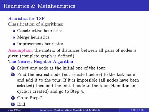
Heuristics & Metaheuristics
Heuristics for TSPClassification of algorithms:
Constructive heuristics.Merge heuristics.Improvement heuristics.
Assumption: the matrix of distances between all pairs of nodes isgiven (complete graph is defined)The Nearest Neighbor Algorithm
1 Select any node as the initial one of the tour.2 Find the nearest node (not selected before) to the last node
and add it to the tour. If it is impossible (all nodes have beenselected) then add the initial node to the tour (Hamiltoniancycle is created) and go to Step 4.
3 Go to Step 2.4 End.
Jan Fábry Advanced Mathematical Models and Methods 137 / 150

Heuristics & Metaheuristics
Savings Algorithm (Clarke and Wright)1 Compute savings
sij = ci1 + c1j � cij fori = 2; 3; : : : ;nj = 2; 3; : : : ;n
i 6= j : (291)
2 Create (n � 1) vehicle routes (1; i ; 1) for i = 2; 3; : : : ;n andorder the savings in a non-increasing fashion.
Parallel version3 (Best feasible merge)
Starting from the top of savings list, execute the following.Given a saving sij , determine whether there exist two routes,one containing arc (1; j ) and the other containing (i ; 1), thatcan feasibly be merged. If so, combine these two routes bydeleting (1; j ) and (i ; 1) and introducing (i ; j ).
Jan Fábry Advanced Mathematical Models and Methods 138 / 150

Heuristics & Metaheuristics
Savings Algorithm (Clarke and Wright)Sequential version
3 (Route extension)Consider the route (1; i ; : : : ; j ; 1). Determine the first savingski or sjl such that k and l are included in other routescontaining arc (k ; 1) or containing arc (1; l).
4 Implement the merge and repeat this operation untilHamiltonian cycle is created.
Insertion Algorithm1 Select any node as the initial one, e.g. node 1.2 Find the farthest node s to the initial one and create the
vehicle route (1; s ; 1).3 Execute the most effective insertion of not-included nodes to
existing route (minimizing the increase of the length of theroute) until Hamiltonian cycle is created.
Jan Fábry Advanced Mathematical Models and Methods 139 / 150

Heuristics & Metaheuristics
Double Spanning-Tree HeuristicLet a complete graph G = fU ;Eg be given.
1 Find the minimal spanning tree G 0 = fU ;E 0g of G.2 Construct the multigraph G� from G 0 by duplicating each arc
from E 0.3 Find an Eulerian cycle Q on G�.4 Delete all node repetitions from Q except for the final return
to the first node. The resulting node sequence T isa Hamiltonian route on G.
Jan Fábry Advanced Mathematical Models and Methods 140 / 150

Heuristics & Metaheuristics
Christofides’ Heuristic (Spanning-Tree/Perfect-Matching)Let a complete graph G = fU ;Eg be given.
1 Find the minimal spanning tree G 0 = fU ;E 0g of G.2 Find the minimal perfect matching on the induced subgraph
G(U0) of G , where U0 � U is the set of nodes of U that areof odd degree in G 0. Let M be the arc set of the perfectmatching.
3 Find an Eulerian cycle Q on the multigraphG� = fU ;E 0 [Mg.
4 Delete all node repetitions from Q except for the final returnto the first node. The resulting node sequence T isa Hamiltonian route on G.
Jan Fábry Advanced Mathematical Models and Methods 141 / 150

Heuristics & Metaheuristics
Cycle Merging HeuristicLet a complete graph G = fU ;Eg be given.
1 Find the initial system of cycles F (e.g. using minimal perfectmatching; if the size of U is odd, one of cycles contains3 nodes).
2 Merge two cycles �� and �� using the following metrics:
D���� = min�;�2F
D�� = mini ;k2�j ;l2�
(cij + ckl � cik � cjl): (292)
Let be the cycle created by merging operation.3 Exclude �� and �� from F , include in F .4 If is not the Hamiltonian cycle then go to Step 2.
Jan Fábry Advanced Mathematical Models and Methods 142 / 150
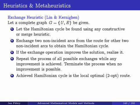
Heuristics & Metaheuristics
Exchange Heuristic (Lin & Kernighen)Let a complete graph G = fU ;Eg be given.
1 Let the Hamiltonian cycle be found using any constructiveor merge heuristic.
2 Exchange two non-incident arcs from the route for other twonon-incident arcs to obtain the Hamiltonian cycle.
3 If the exchange operation improves the solution, realize it.4 Repeat the process of all possible exchanges while any
improvement is achieved. Terminate the process when noimprovement is possible.
5 Achieved Hamiltonian cycle is the local optimal (2-opt) route.
Jan Fábry Advanced Mathematical Models and Methods 143 / 150

Heuristics & Metaheuristics
MetaheuristicsNotation in algorithms:x is a feasible solution to the given problemX is a feasible solution space, i.e. a set of all xN (x ) is a neighborhood of solution x (a set of close solutions)f (x ) is a minimization objective functionx � is the currently best found solutionLocal Search (LS)
1 Choose an initial solution x 2 X and set x � = x .2 Define the neighborhood N (x ) � X and evaluate all solutions.3 Let x 0 be the best solution from N (x ).
If f (x 0) < f (x �) then set x � = x 0 and x = x 0, stop otherwise.4 If the stopping rule is not met go to Step 2.5 Solution x � is a local minimum solution.
Jan Fábry Advanced Mathematical Models and Methods 144 / 150
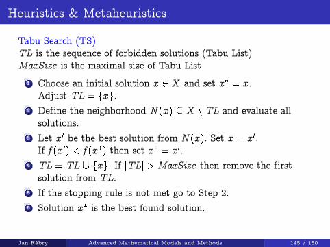
Heuristics & Metaheuristics
Tabu Search (TS)TL is the sequence of forbidden solutions (Tabu List)MaxSize is the maximal size of Tabu List
1 Choose an initial solution x 2 X and set x � = x .Adjust TL = fxg.
2 Define the neighborhood N (x ) � X nTL and evaluate allsolutions.
3 Let x 0 be the best solution from N (x ). Set x = x 0.If f (x 0) < f (x �) then set x � = x 0.
4 TL = TL[ fxg. If jTLj > MaxSize then remove the firstsolution from TL.
5 If the stopping rule is not met go to Step 2.6 Solution x � is the best found solution.
Jan Fábry Advanced Mathematical Models and Methods 145 / 150

Heuristics & Metaheuristics
Threshold Accepting Algorithm (TA)T is the threshold value for accepting worse solutionsT0 is the initial value of thresholdr 2 (0; 1) is the rate of threshold reduction
1 Choose an initial solution x 2 X and set x � = x .Adjust T = T0.
2 Repeat n-times:I choose x 0 2 N (x ),I if f (x 0)�T < f (x ) then x = x 0,I if f (x 0) < f (x �) then x � = x 0.
3 If the stopping rule is not met then execute the reductionT = rT and go to Step 2.
4 Solution x � is the best found solution.
Jan Fábry Advanced Mathematical Models and Methods 146 / 150

Heuristics & Metaheuristics
Simulated Annealing Method (SIAM)T is the temperature valueT0 is the initial temperature valuer 2 (0; 1) is the rate of temperature reduction (cooling rate)
1 Choose an initial solution x 2 X and set x � = x .Adjust T = T0.
2 Repeat n-times:I choose x 0 2 N (x ),I if f (x 0) < f (x ) then x = x 0,I if f (x 0) � f (x ) then x = x 0 with the probability e�
�
T , where� = f (x 0)� f (x ),
I if f (x 0) < f (x �) then x � = x 0.3 If the stopping rule is not met (or the process has not yet
frozen) then execute the reduction T = rT and go to Step 2.4 Solution x � is the best found solution.
Jan Fábry Advanced Mathematical Models and Methods 147 / 150
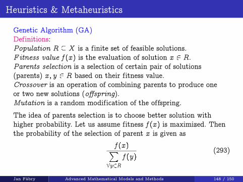
Heuristics & Metaheuristics
Genetic Algorithm (GA)Definitions:Population R � X is a finite set of feasible solutions.Fitness value f (x ) is the evaluation of solution x 2 R.Parents selection is a selection of certain pair of solutions(parents) x ; y 2 R based on their fitness value.Crossover is an operation of combining parents to produce oneor two new solutions (offspring).Mutation is a random modification of the offspring.
The idea of parents selection is to choose better solution withhigher probability. Let us assume fitness f (x ) is maximized. Thenthe probability of the selection of parent x is given as
f (x )X8y2R
f (y)(293)
Jan Fábry Advanced Mathematical Models and Methods 148 / 150

Heuristics & Metaheuristics
Genetic Algorithm (GA)Let parent x be encoded as x1x2 : : : xr , parent y be encoded asy1y2 : : : yr and child z be encoded as z1z2 : : : zr .
Crossover of parentsI 1-point crossover
Child #1: x1 : : : xpyp+1 : : : yr ,Child #2: y1 : : : ypxp+1 : : : xr .
I 2-point crossoverChild #1: x1 : : : xpyp+1 : : : yqxq+1 : : : xr ,Child #2: y1 : : : ypxp+1 : : : xqyq+1 : : : yr .
I Uniform crossoverChild: z1z2 : : : zr , where zi 2 fxi ; yig; i = 1; 2; : : : ; r .
Mutation of a childI 1-point mutation
Modified child: z1 : : : zp�1z �p zp+1 : : : zr , where z �p 6= zp .I 2-point mutation
Modified child: z1 : : : zp�1zqzp+1 : : : zq�1zpzq+1 : : : zr .
Jan Fábry Advanced Mathematical Models and Methods 149 / 150

Heuristics & Metaheuristics
Ant Colony Optimization (ACO)
The method is based on swarm intelligence.Each ant tries to find a route between its nest and a foodsource.On the path, ants lay down a pheromone trail.Ants prefer to take those paths where there is a larger amountof pheromone.The pheromone trails on the longer paths evaporate fasterthan on the shorter paths.Pheromone evaporation also has the advantage of avoiding theconvergence to a local optimal solution.The idea of the ACO is to mimic this behavior with “simulatedants” (agents) walking around the graph representing theproblem to solve.
Jan Fábry Advanced Mathematical Models and Methods 150 / 150