Advanced Machine LearningPractical 3: Classification (SVM, RVM & AdaBoost)

Professor: Aude BillardAssistants: Guillaume de Chambrier,Nadia Figueroa and Denys Lamotte

Spring Semester 2016

1 Introduction

During this week’s practical we will focus on understanding and comparing the perfor-mance of the different classification methods seen in class, namely SVM and its variants(C-SVM and ν-SVM, RVM) and an instance of a Boosting method, specifically AdaBoost.

In non-linear classification methods such as SVM/RVM, we seek to find the optimalhyper-parameters (C: penalty, ν: bounds, σ: kernel width for RBF) which will optimizethe objective function (and consequently the parameters of the class decision function).Choosing the best hyper-parameters for your dataset is not a trivial task, we will analyzetheir effect on the classifier and how to choose an admissible range of parameters. Astandard way of finding these optimal hyper-parameters is by doing a grid search, i.e.systematically evaluating each possible combination of parameters within a given range.We will do this for different datasets and discuss the difference in performance, modelcomplexity and sensitivity to hyper-parameters.

On the other hand, Boosting chooses weak classifiers (WC) iteratively among a largeset of randomly created WC and combines them to create a strong classifier, by increasingthe weights of datapoints not well classified by the previous combination of WC.

We will compare the performance of SVM vs. Adaboost (with decision stumps as theWC) on multiple datasets. We will also evaluate which method is more reliable whenhandling noisy data, data with outliers and data with unbalanced classes.

2 ML toolbox

ML toolbox contains a set of matlab methods and examples for learning about machinelearning methods. You can download ML toolbobx from here: [link] and the matlabscripts for this tutorial from here [link]. The matlab scripts will make use of the toolbox.

Before proceeding make sure that all the sub-directories of the ML toolbox includingthe files in TP3 have been added to your matlab search path. This can be done as followsin the matlab command window:

1

>> addpath(genpath(’path to ML toolbox’))>> addpath(genpath(’path to TP3’))

To test that all is working properly you can try out some examples of the toolbox;look in the examples sub-directory.

3 Support Vector Machines (SVM)

SVM is one of the most powerful non-linear classification methods to date, as it is able tofind a separating hyper-plane for non-seperable data on a high-dimensional feature spaceusing the kernel trick. Yet, in order for it to perform as expected, we need to find the ’best’hyper-parameters given the dataset at hand. In this section we will compare its variants(C-SVM, ν-SVM) and get an underlying intuition of the effects of its hyper-parametersand how to choose them.

3.1 C-SVM

Given a data set (x1, y1), . . . , (xM , yM) of M samples in which the class label yi ∈{−1,+1} is either positive or negative, SVM seeks to optimize the following optimizationproblem for such binary classification task.

minw,ξ

(1

2||w||2 +

C

M

M∑i=1

ξi

)s.t. yi(〈wT ,xi〉+ b) ≥ 1− ξiξi ≥ 0 ∀i = 1, . . .M

(1)

where w is the separating hyper-plane, ξi are the slack variables, b is the bias and C is themisclassification penalty factor used to find a trade-off between maximizing the marginand minimizing classification errors. This yields a decision function y(x)→ {−1,+1} ofthe following form:

y(x) = sign(〈wT ,xi〉+ b

)= sign

(M∑i=1

αiyi〈wT ,xi〉+ b

)(2)

where αi are the Lagrangian multipliers which define the support vectors (α > 0 aresupport vectors). As seen in class, instead of transforming the data to a high-dimensionalfeature space, we use the inner product of the feature space, this is the so-called kerneltrick, the decision function then becomes:

y(x) = sign

(M∑i=1

αmyi k(x,xi) + b

)(3)

where k(x,xi) is the kernel function, which will be the Radial Basis function for thistutorial. The parameters for this decision function are learned by solving the Lagrangiandual of the optimization problem (Eq. 1) in feature space, this was seen in class and willnot be covered here. There are extensions such to be able to handle multi-class problems,but in this tutorial we will be focusing on the binary case.

2

Kernels SVM has the flexibility to handle many types of kernels, we have three optionsimplemented in ML toolbox:

• Homogeneous Polynomial: k(x,xi) = (〈x,x〉)p,where p < 0 and corresponds to the polynomial degree.

• Inhomogeneous Polynomial: k(x,xi) = (〈x,x + d〉)p,where p < 0 and corresponds to the polynomial degree and d ≥ 0, generally d = 1.

• Radial Basis Function (Gaussian): k(x,xi) = exp{− 1

2σ2 ||x− xi||2}

,where σ is the width or scale of the Gaussian kernel centered at xi

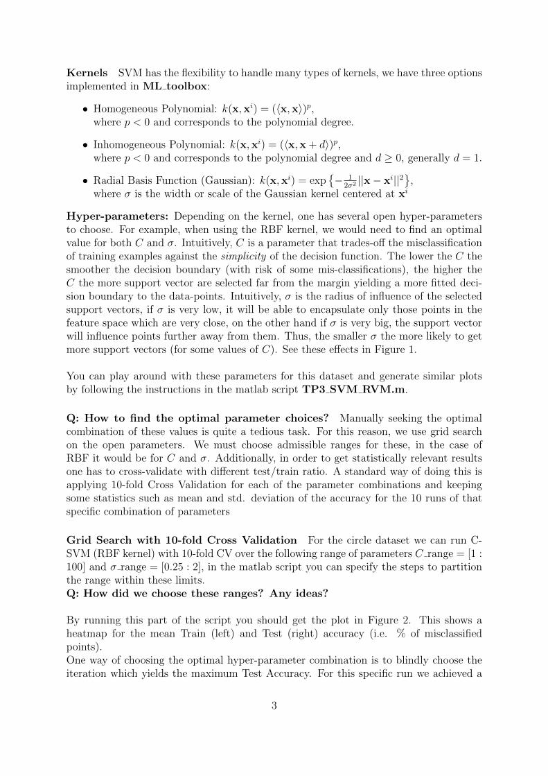
Hyper-parameters: Depending on the kernel, one has several open hyper-parametersto choose. For example, when using the RBF kernel, we would need to find an optimalvalue for both C and σ. Intuitively, C is a parameter that trades-off the misclassificationof training examples against the simplicity of the decision function. The lower the C thesmoother the decision boundary (with risk of some mis-classifications), the higher theC the more support vector are selected far from the margin yielding a more fitted deci-sion boundary to the data-points. Intuitively, σ is the radius of influence of the selectedsupport vectors, if σ is very low, it will be able to encapsulate only those points in thefeature space which are very close, on the other hand if σ is very big, the support vectorwill influence points further away from them. Thus, the smaller σ the more likely to getmore support vectors (for some values of C). See these effects in Figure 1.

You can play around with these parameters for this dataset and generate similar plotsby following the instructions in the matlab script TP3 SVM RVM.m.

Q: How to find the optimal parameter choices? Manually seeking the optimalcombination of these values is quite a tedious task. For this reason, we use grid searchon the open parameters. We must choose admissible ranges for these, in the case ofRBF it would be for C and σ. Additionally, in order to get statistically relevant resultsone has to cross-validate with different test/train ratio. A standard way of doing this isapplying 10-fold Cross Validation for each of the parameter combinations and keepingsome statistics such as mean and std. deviation of the accuracy for the 10 runs of thatspecific combination of parameters

Grid Search with 10-fold Cross Validation For the circle dataset we can run C-SVM (RBF kernel) with 10-fold CV over the following range of parameters C range = [1 :100] and σ range = [0.25 : 2], in the matlab script you can specify the steps to partitionthe range within these limits.Q: How did we choose these ranges? Any ideas?

By running this part of the script you should get the plot in Figure 2. This shows aheatmap for the mean Train (left) and Test (right) accuracy (i.e. % of misclassifiedpoints).One way of choosing the optimal hyper-parameter combination is to blindly choose theiteration which yields the maximum Test Accuracy. For this specific run we achieved a

3

(a) Concentric Circle Classifica-tion Problem (500 datapoints)

(b) C=1, σ=0.75, SV=59 (c) C=500, σ=0.75, SV=19

(d) C=1000, σ=0.75, SV=17 (e) C=100, σ=0.25, SV=138 (f) C=100, σ=2, SV=24

Figure 1: Decision Boundaries with different hyper-parameter values for the circle dataset.Support Vector: data-points with white edges.

Max. Test Accuracy of 98.7% with C = 1, σ = 1.72, by plotting the decision boundarywe get the plot in Figure 3.

As can be seen, the classifier does recover the circular shape of the real boundary fromthe dataset. However, if we take a look at the support vectors, there seems to be manyand quite close to each other.

Q: Could there be a way to recover a similar decision boundary with lesssupport vectors? Let’s take a look back at the heatmap for Test Mean accuracy(Figure 2). The max accuracy was chosen from a very tiny white area close to the x-axisof the heatmap. We can see that there is a bigger region with really high accuracy on thebottom-right corner of the heatmap where the C value is not so close to 0. Intuitively,if σ is larger, we should have less support vectors, so, let’s choose the mid-point of thisarea which gives us C = 10, σ = 1.9, this yields the decision boundary seen in Figure 4,and from our initial guess, we indeed recover the same decision boundary with less thanhalf the amount of support vectors (SV=38) than before.

Q: Why should we seek for the least number of support vectors? The numberof support vectors needed to recover the decision boundary for our classifier is in fact themeasure of model complexity for SVMs.

4

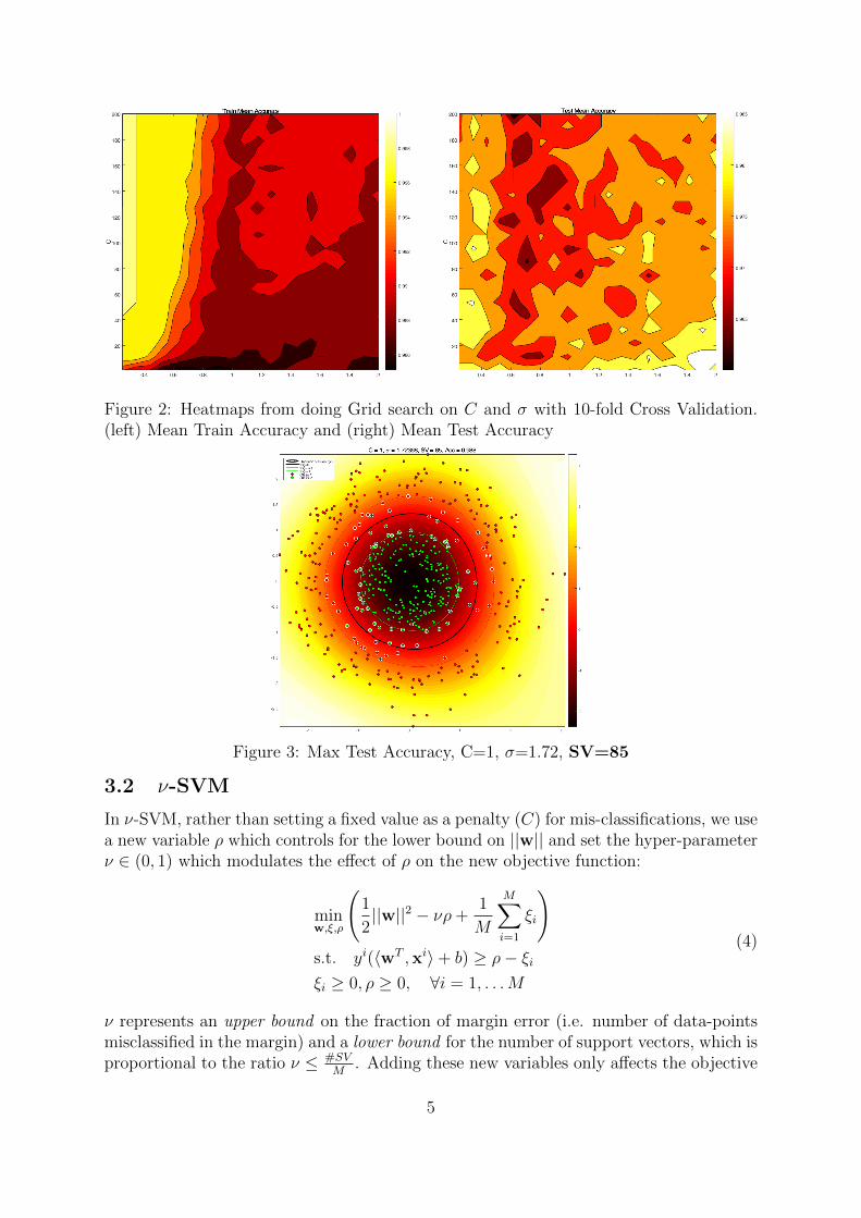
Figure 2: Heatmaps from doing Grid search on C and σ with 10-fold Cross Validation.(left) Mean Train Accuracy and (right) Mean Test Accuracy

Figure 3: Max Test Accuracy, C=1, σ=1.72, SV=85

3.2 ν-SVM

In ν-SVM, rather than setting a fixed value as a penalty (C) for mis-classifications, we usea new variable ρ which controls for the lower bound on ||w|| and set the hyper-parameterν ∈ (0, 1) which modulates the effect of ρ on the new objective function:

minw,ξ,ρ

(1

2||w||2 − νρ+

1

M

M∑i=1

ξi

)s.t. yi(〈wT ,xi〉+ b) ≥ ρ− ξiξi ≥ 0, ρ ≥ 0, ∀i = 1, . . .M

(4)

ν represents an upper bound on the fraction of margin error (i.e. number of data-pointsmisclassified in the margin) and a lower bound for the number of support vectors, which isproportional to the ratio ν ≤ #SV

M. Adding these new variables only affects the objective

5

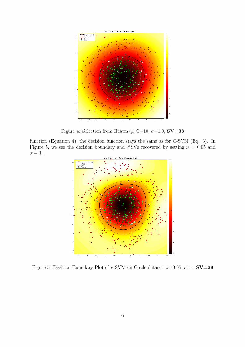
Figure 4: Selection from Heatmap, C=10, σ=1.9, SV=38

function (Equation 4), the decision function stays the same as for C-SVM (Eq. 3). InFigure 5, we see the decision boundary and #SVs recovered by setting ν = 0.05 andσ = 1.

Figure 5: Decision Boundary Plot of ν-SVM on Circle dataset, ν=0.05, σ=1, SV=29

6

3.3 Relevance Vector Machines (RVM)

The Relevance Vector Machine (RVM) applies the Bayesian ’Automatic Relevance De-termination’ (ARD) methodology to linear kernel models, which have a very similarformulation to the SVM, hence, it is considered as sparse SVM. When predictive modelsare linear in parameters, ARD can be used to infer a flexible, non-linear, predictive modelwhich is both accurate and uses a very small number of relevant basis functions (in ourcase support vectors) from a large initial set. The predictive linear model for RVM hasthe following form:

y(x) =M∑i=1

αi k(x,xi) = αTΨ(x) (5)

where Ψ(x) = [Ψ0(x), . . . ,ΨM(x), ]T is a linear combination of basis functions Ψ(x) =k(x,xi), α = [1, 0, 1, 0, , . . . 0, 0, 0, 1] is a sparse vector of weights and y(x) is the binaryclassification decision function y(x) → {1, 0}. The problem in RVM is now to find asparse solution for α, where αi = 1 when the datapoint is a relevant ’support’ vector and0 otherwise. Finding such a sparse solution is not trivial. ARD is a method tailor-madeto discover the relevance of parameters for a predictive model by imposing a prior on theparameter whose relevance needs to be determined. When attempting to calculate α wetake a Bayesian approach and assume that all output labels yi are i.i.d samples from atrue model y(xi) (Equation 5) subject to some Gaussian noise with zero-mean:

yi(x) = y(xi) + ε

= αTΨ(xi) + ε(6)

where ε ∝ N (0, σ2ε ). We can then estimate the probability of a label yi given x with a

Gaussian distribution with mean on y(xi) and variance σ2ε , this is equivalent to:

p(yi|x) = N (yi|y(xi), σ2ε )

= (2πσ2ε )

− 12 exp

{− 1

2σ2ε

(yi − y(xi)2}

= (2πσ2ε )

− 12 exp

{− 1

2σ2ε

(yi − αTΨ(xi))2} (7)

Thanks to the independence assumption we can then estimate the likelihood of the com-plete dataset with the following form:

p(y|x, σ2ε ) = (2πσ2

ε )−M

2 exp

{− 1

2σ2ε

||y − αTΨ(x)||2}

(8)

We could then approximate α and σ2ε through MLE (Maximum Likelihood Estimation),

however, this would not yield a sparse vector α, instead it would give us an over-fittingmodel, setting each point as a relevant basis function. To impose sparsity on the solution,we define an explicit prior probability distribution over α, namely a zero-mean Gaussian:

p(α|a) =M∏i=0

N (αi|0, a−1i ) (9)

7

where a = [a0, . . . , aM ] is a vector of hyper-parameters ai, each corresponding to anindependent weight αi indicating it’s strength (or relevance). For the binary classificationproblem, rather than predicting a discriminative membership of a class y → {1, 0}, inRVM we predict the posterior probability P (y|x) of one class y ∈ {1, 0} given input x bygeneralizing the linear model from Equation 5 with the logistic sigmoid function σ(y) ofthe form:

σ(y) =1

1 + exp{−y}(10)

The Bernoulli distribution is used for P (y|x) and the likelihood then becomes:

P (y|α) =M∏i=1

σ{y(xi)}yi [1− σ{y(xi)}]1−yi (11)

Now, following Bayesian inference, to learn the unknown hyper-parameters α, a we startwith the decomposed posterior1 over unknowns given the data:

p(α, a, |y) = p(α|y, a)p(a|y) (12)

where unfortunately the posterior distribution over the weights p(α|y, a) and the hyper-parameter posterior p(a|y) are not analytically solvable. It can however be approximatedby using Laplace’s method2. Estimating for α then becomes a problem of maximizingthe weight posterior distribution p(α|y, a), and since p(α|y, a) ∝ P (y|α)p(α|a) (whichare Equations 11 and 9 corresponding to the likelihood and prior of the weights α) thisis equivalent to maximizing the following equation over α:

log{P (y|α)p(α|a)} =M∑i=1

[yi log σ{y(xi)}+ (1− yi) log(1− σ{y(xi)})]− 1

2αTAα (13)

where A = diag(a0, . . . , aM). This is optimized in an iterative procedure, a is updatedin each step following some derivations from Tipping. Once we have learned our hyper-parameters, Equation 11 is then used to estimate probabilities for each class, in thebinary case when p(y|x) = 0.5 this corresponds to the decision boundary, values ≥ 0.5correspond to the positive class and consequently < 0.5 to the negative class.

As in SVM, the basis functions for the linear model Ψi(x) = k(x,xi) can be any typeof kernel, in this tutorial we will consider only RBF for the RVM. In Figure 6, we seethe decision boundary and #RVs recovered by setting σ = 1.22 found through 10-foldCross-Validation.

1Refer to the Tipping’s paper on RVM to understand how this and subsequent terms were derived.Tipping, M. E. (2001). Sparse Bayesian learning and the relevance vector machine. Journal of MachineLearning Research 1, 211–244.

2Refer to Tipping paper for Laplace’s Approximation.

8

3.4 Objectives

• Follow the same evaluation as the one done for C-SVM with ν-SVM and RVM on thedifferent datasets (Figure 7) available in the matlab script TP3 SVM RVM.m.

• Try out different kernels and evaluate their performance or feasibility depending onthe dataset.

• Do grid search for C-SVM, ν-SVM and RVM

• Find the admissible range of parameters for each dataset and for each method.

Figure 6: Decision Boundary Plot of RVM on Circle dataset, σ=1.22, RV=4

(a) Checkerboard Dataset (b) Very non-linear dataset (c) Ripley Dataset

Figure 7: Datasets to evaluate C-SVM, ν-SVM and RVM .

9

4 AdaBoost

AdaBoost iteratively builds a strong classifier from a set of weak classifiers. The finalstrong classifier is a weighted linear combination of simple, also known as weak classifiersφ(x)→ {−1,+1}, into a strong classifier, C(x)→ {−1,+1}.

The original formulation of AdaBoost considers binary classification problems. Thereare extensions such to be able to handle multi-class problems, but in this tutorial we willbe focusing on the binary case. Given a data set (x1, y1), . . . , (xm, ym) of m samples inwhich the class label yi ∈ {−1,+1} is either positive or negative we seek to learn a strongclassifier C(x), Equation 14,

C(x) = sign

(M∑m=1

αm φ(xm)

), αm ∈ R (14)

In theory you can use any classifier for φ(xm), but usually it should be a very simpleand cheap to compute. In this tutorial we will be consider decision stumps, Equation15, as the weak classifier:

φ(x; θ) =

{+1 if xθ1 > θ2

−1 otherwise(15)

A decision stump in function which separates the classes along a dimension. It has twoparameters θ = {θ1, θ2}. The first parameter indicates in which dimension the decisionboundary will be placed and the second parameter decides where along this dimensiondoes the split occur.

To understand the mechanism for Boosting methods we will study how a strongclassifier is learned for the circle dataset used in the previous section. The classes arenon-linearly separable, in the previous tutorial we used kPCA to find a projection forwhich the data was linearly separable. This was one approach, now we will proceed tolearn a set of linear classifiers which when combined will result in a non-linear classifier.

In Figure 8(a)-8(b) the result of AdaBoost when only one weak classifier is used; weclearly see the decision stump. The figure on the right illustrate the non-signed outputof Equation 14 and the figure on the left is the result after taking the sign. Points whichare misclassified have a cross on them, but in addition you will see that the width of thedata points have changed (Left column). The width of a data point is proportional tothe weight given by the AdaBoost algorithm.

In the second iteration, the number of weak classifiers goes from one to two. Thesecond decision stump is trained on the new weighted dataset, for which there clas-sification error from points which high weights are consider more important than datapoints with low weights. After the 50 iterations (thus 50 weak classifiers), a nearly perfectclassification is achieved, see Figure 8(e)-8(f).

10

(a) (b)

(c) (d)

(e) (f)

Figure 8: AdaBoost applied to the circle data set. Width of circles on the Left columnare proportional to the classification error and the crosses depict the points which havebeen misclassified. In the Right column, the value is of the strong classifier function C(x)before the sign operator is applied.

11

Figure 9: AdaBoost, 10-fold CV over an increasing number of weak classifiers; for thecircle data set. The accuracy for both the train (green) and test (red) data sets areshown.

10-fold Cross Validation Run AdaBoost with 10-fold CV over the range of parame-ters specified in the matlab script file TP3 Boosting.m. You should get the followingplot, Figure 9. You can see that the test error after 40 decision stumps has settled ataround a 90%.

4.1 Objectives

• Follow the same evaluation for the different datasets available used in the SVmevaluation (Figure 7) in the matlab script TP3 Boosting.m.

This is all good, however the original AdaBoost algorithm can be sensitive to noise,which will study next.

4.2 Comparison SVM VS AdaBoost

Sensitivity to noise in comparison to C-SVM AdaBoost is known to be very sen-sitive to noise. Indeed it has been proved that the objective of AdaBoost is to minimizethe exponential loss (

∑i

e−yiφ(xi)) of the combined classifier on the training data. As

penalties for misclassification grow exponentially with the magnitude of the predictivefunction output, outlier points could have a very strong influence on the final learnedmodel and so make it very sensitive to noisy data/outliers.

12

In order to see this you can run these examples in TP3 SVM Boosting.m. In thisscript, you will see that there is the possibility to add noise in the previously used datasetsin different ways :

Figure 10: C-SVM and AdaBoost, 10-fold CV over an increasing percentage of noisy datafor the circle data set. The accuracy for both the train and test data sets are shown.

• Adding some outliers in the dataset (points which are in the region of some classbut with a wrong label). This can be seen as class noise.

• Adding noisy data in the dataset (points in each class whose attributes are chosenrandomly). This is attribute noise.

• Unbalancing the dataset (one of the class contains more samples than the other(s)).

If we perform a 10-fold cross validation on these modified datasets, using C-SVM and Ad-aBoost for comparison, we should be able to see that the accuracy of Adaboost decreasesmore than the one of SVM if we add some noise in the data. See Figure 10.

4.3 Objectives

• Evalute the accuracy for the different datasets (Figure 7) available in thematlab script TP3 SVM Boosting.m (Figure 7).

• Do the 10-fold cross validation for both C-SVM and AdaBoost choosing the optimalhyperparameters found before on the original dataset and compare the performance.

• Try adding different types of noise to the dataset as mentionned before.

• Compare again the accuracy of C-SVM and AdaBoost on these modified datasets.You can can also compare the evolution of it by increasing the percentage ofnoisy/outlier/unbalanced data.

13