Advanced Linear Algebra - GitHub Pages · 1.1.1. Introduction to Advanced Linear Algebra Advanced...
180
Advanced Linear Algebra MAT3040 Notebook The First Edition
Transcript of Advanced Linear Algebra - GitHub Pages · 1.1.1. Introduction to Advanced Linear Algebra Advanced...

Advanced Linear Algebra
MAT3040 Notebook
The First Edition

A FIRST COURSE
IN
ADVANCED LINEAR ALGEBRA


A FIRST COURSE
IN
ADVANCED LINEAR ALGEBRA
MAT3040 Notebook
Lecturer
Prof. Daniel Wong
The Chinese University of Hongkong, Shenzhen
Tex Written By
Mr. Jie Wang
The Chinese University of Hongkong, Shenzhen


Contents
1 Week1 . . . . . . . . . . . . . . . . . . . . . . . . . . . . . . . . . . . . . . . . . . . . . . . . . . . . . . 1
1.1 Monday for MAT3040 1
1.1.1 Introduction to Advanced Linear Algebra . . . . . . . . . . . . . . . . . . . . . . . . . . . . . . . . 1
1.1.2 Vector Spaces . . . . . . . . . . . . . . . . . . . . . . . . . . . . . . . . . . . . . . . . . . . . . . . . . . . 2
1.4 Wednesday for MAT3040 14
1.4.1 Review . . . . . . . . . . . . . . . . . . . . . . . . . . . . . . . . . . . . . . . . . . . . . . . . . . . . . . . . 14
1.4.2 Spanning Set . . . . . . . . . . . . . . . . . . . . . . . . . . . . . . . . . . . . . . . . . . . . . . . . . . . 14
1.4.3 Linear Independence and Basis . . . . . . . . . . . . . . . . . . . . . . . . . . . . . . . . . . . . . . . 16
2 Week2 . . . . . . . . . . . . . . . . . . . . . . . . . . . . . . . . . . . . . . . . . . . . . . . . . . . . . 33
2.1 Monday for MAT3040 33
2.1.1 Basis and Dimension . . . . . . . . . . . . . . . . . . . . . . . . . . . . . . . . . . . . . . . . . . . . . . 33
2.1.2 Operations on a vector space . . . . . . . . . . . . . . . . . . . . . . . . . . . . . . . . . . . . . . . . 36
2.4 Wednesday for MAT3040 51
2.4.1 Remark on Direct Sum . . . . . . . . . . . . . . . . . . . . . . . . . . . . . . . . . . . . . . . . . . . . . 51
2.4.2 Linear Transformation . . . . . . . . . . . . . . . . . . . . . . . . . . . . . . . . . . . . . . . . . . . . . 52
3 Week3 . . . . . . . . . . . . . . . . . . . . . . . . . . . . . . . . . . . . . . . . . . . . . . . . . . . . . 73
3.1 Monday for MAT3040 73
3.1.1 Remarks on Isomorphism . . . . . . . . . . . . . . . . . . . . . . . . . . . . . . . . . . . . . . . . . . . 73
3.1.2 Change of Basis and Matrix Representation . . . . . . . . . . . . . . . . . . . . . . . . . . . . . . 74
3.4 Wednesday for MAT3040 92
3.4.1 Remarks for the Change of Basis . . . . . . . . . . . . . . . . . . . . . . . . . . . . . . . . . . . . . . 92
4 Week4 . . . . . . . . . . . . . . . . . . . . . . . . . . . . . . . . . . . . . . . . . . . . . . . . . . . . 109
4.1 Monday for MAT3040 109
4.1.1 Quotient Spaces . . . . . . . . . . . . . . . . . . . . . . . . . . . . . . . . . . . . . . . . . . . . . . . . 109
4.1.2 First Isomorphism Theorem . . . . . . . . . . . . . . . . . . . . . . . . . . . . . . . . . . . . . . . . . 112
1

4.4 Wednesday for MAT3040 126
4.4.1 Dual Space . . . . . . . . . . . . . . . . . . . . . . . . . . . . . . . . . . . . . . . . . . . . . . . . . . . . 131
5 Week5 . . . . . . . . . . . . . . . . . . . . . . . . . . . . . . . . . . . . . . . . . . . . . . . . . . . . 145
5.1 Monday for MAT3040 145
5.1.1 Remarks on Dual Space . . . . . . . . . . . . . . . . . . . . . . . . . . . . . . . . . . . . . . . . . . . 146
5.1.2 Annihilators . . . . . . . . . . . . . . . . . . . . . . . . . . . . . . . . . . . . . . . . . . . . . . . . . . . 148
5.4 Wednesday for MAT3040 160
5.4.1 Adjoint Map . . . . . . . . . . . . . . . . . . . . . . . . . . . . . . . . . . . . . . . . . . . . . . . . . . . 161
5.4.2 Relationship between Annihilator and dual of quotient spaces . . . . . . . . . . . . . . . . . 163
6 Week6 . . . . . . . . . . . . . . . . . . . . . . . . . . . . . . . . . . . . . . . . . . . . . . . . . . . . 175
6.1 Monday for MAT3040 175
6.1.1 Polynomials . . . . . . . . . . . . . . . . . . . . . . . . . . . . . . . . . . . . . . . . . . . . . . . . . . . 175
6.4 Wednesday for MAT3040 185
6.4.1 Eigenvalues & Eigenvectors . . . . . . . . . . . . . . . . . . . . . . . . . . . . . . . . . . . . . . . . . 188
7 Week7 . . . . . . . . . . . . . . . . . . . . . . . . . . . . . . . . . . . . . . . . . . . . . . . . . . . . 193
7.1 Monday for MAT3040 193
7.1.1 Minimal Polynomial . . . . . . . . . . . . . . . . . . . . . . . . . . . . . . . . . . . . . . . . . . . . . . 193
7.1.2 Minimal Polynomial of a vector . . . . . . . . . . . . . . . . . . . . . . . . . . . . . . . . . . . . . . 198
7.4 Wednesday for MAT3040 211
7.4.1 Cayley-Hamiton Theorem . . . . . . . . . . . . . . . . . . . . . . . . . . . . . . . . . . . . . . . . . . 211
8 Week8 . . . . . . . . . . . . . . . . . . . . . . . . . . . . . . . . . . . . . . . . . . . . . . . . . . . . 225
8.1 Monday for MAT3040 225
8.1.1 Cayley-Hamiton Theorem . . . . . . . . . . . . . . . . . . . . . . . . . . . . . . . . . . . . . . . . . . 227
8.1.2 Primary Decomposition Theorem . . . . . . . . . . . . . . . . . . . . . . . . . . . . . . . . . . . . . 230
2
9 Week9 . . . . . . . . . . . . . . . . . . . . . . . . . . . . . . . . . . . . . . . . . . . . . . . . . . . . 251
9.1 Monday for MAT3040 251
9.1.1 Remarks on Primary Decomposition Theorem . . . . . . . . . . . . . . . . . . . . . . . . . . . . 251
9.4 Wednesday for MAT3040 268
9.4.1 Jordan Normal Form . . . . . . . . . . . . . . . . . . . . . . . . . . . . . . . . . . . . . . . . . . . . . 268
9.4.2 Inner Product Spaces . . . . . . . . . . . . . . . . . . . . . . . . . . . . . . . . . . . . . . . . . . . . . 273
10 Week10 . . . . . . . . . . . . . . . . . . . . . . . . . . . . . . . . . . . . . . . . . . . . . . . . . . . 285
10.1 Monday for MAT3040 285
10.1.1 Inner Product Space . . . . . . . . . . . . . . . . . . . . . . . . . . . . . . . . . . . . . . . . . . . . . 285
10.1.2 Dual spaces . . . . . . . . . . . . . . . . . . . . . . . . . . . . . . . . . . . . . . . . . . . . . . . . . . . 288
10.4 Wednesday for MAT3040 297
10.4.1 Orthogonal Complement . . . . . . . . . . . . . . . . . . . . . . . . . . . . . . . . . . . . . . . . . . . 297
10.4.2 Adjoint Map . . . . . . . . . . . . . . . . . . . . . . . . . . . . . . . . . . . . . . . . . . . . . . . . . . . 300
11 Week11 . . . . . . . . . . . . . . . . . . . . . . . . . . . . . . . . . . . . . . . . . . . . . . . . . . . 315
11.1 Monday for MAT3040 315
11.1.1 Self-Adjoint Operator . . . . . . . . . . . . . . . . . . . . . . . . . . . . . . . . . . . . . . . . . . . . . 315
11.1.2 Orthononal/Unitary Operators . . . . . . . . . . . . . . . . . . . . . . . . . . . . . . . . . . . . . . 318
11.4 Wednesday for MAT3040 332
11.4.1 Unitary Operator . . . . . . . . . . . . . . . . . . . . . . . . . . . . . . . . . . . . . . . . . . . . . . . . 332
11.4.2 Normal Operators . . . . . . . . . . . . . . . . . . . . . . . . . . . . . . . . . . . . . . . . . . . . . . . 335
12 Week12 . . . . . . . . . . . . . . . . . . . . . . . . . . . . . . . . . . . . . . . . . . . . . . . . . . . 349
12.1 Monday for MAT3040 349
12.1.1 Remarks on Normal Operator . . . . . . . . . . . . . . . . . . . . . . . . . . . . . . . . . . . . . . . 349
12.1.2 Tensor Product . . . . . . . . . . . . . . . . . . . . . . . . . . . . . . . . . . . . . . . . . . . . . . . . . 353
12.4 Wednesday for MAT3040 367
12.4.1 Introduction to Tensor Product . . . . . . . . . . . . . . . . . . . . . . . . . . . . . . . . . . . . . . 367
3

13 Week13 . . . . . . . . . . . . . . . . . . . . . . . . . . . . . . . . . . . . . . . . . . . . . . . . . . . 381
13.1 Monday for MAT3040 381
13.1.1 Basis of V ⌦ W . . . . . . . . . . . . . . . . . . . . . . . . . . . . . . . . . . . . . . . . . . . . . . . . . 383
13.1.2 Tensor Product of Linear Transformation . . . . . . . . . . . . . . . . . . . . . . . . . . . . . . . 387
13.4 Wednesday for MAT3040 399
13.4.1 Tensor Product for Linear Transformations . . . . . . . . . . . . . . . . . . . . . . . . . . . . . . 399
14 Week14 . . . . . . . . . . . . . . . . . . . . . . . . . . . . . . . . . . . . . . . . . . . . . . . . . . . 417
14.1 Monday for MAT3040 417
14.1.1 Multilinear Tensor Product . . . . . . . . . . . . . . . . . . . . . . . . . . . . . . . . . . . . . . . . . 417
14.1.2 Exterior Power . . . . . . . . . . . . . . . . . . . . . . . . . . . . . . . . . . . . . . . . . . . . . . . . . 420
15 Week15 . . . . . . . . . . . . . . . . . . . . . . . . . . . . . . . . . . . . . . . . . . . . . . . . . . . 431
15.1 Monday for MAT3040 431
15.1.1 More on Exterior Power . . . . . . . . . . . . . . . . . . . . . . . . . . . . . . . . . . . . . . . . . . . 431
15.1.2 Determinant . . . . . . . . . . . . . . . . . . . . . . . . . . . . . . . . . . . . . . . . . . . . . . . . . . . 433
4
Acknowledgments
This book is taken notes from the MAT3040 in spring semester, 2019. These lecture notes
were taken and compiled in LATEX by Jie Wang, an undergraduate student in spring
2019. The tex writter would like to thank Prof. Daniel Wong and some students for
their detailed and valuable comments and suggestions, which significantly improved
the quality of this notebook. Students taking this course may use the notes as part of
their reading and reference materials. This version of the lecture notes were revised and
extended for many times, but may still contain many mistakes and typos, including
English grammatical and spelling errors, in the notes. It would be greatly appreciated
if those students, who will use the notes as their reading or reference material, tell any
mistakes and typos to Jie Wang for improving this notebook.
xv


Notations and Conventions
Fn n-dimensional F-valued space
Mm⇥n(F) set of all m ⇥ n F-valued matrices
� Direct Sum
ker(T) The null space of T
V �W vector spaces V and W are isomorphic
(T)B,A Matrix representation of T w.r.t. A and B
vvv +W coset of vvv, i.e., {vvv + www | www 2 W}
aaaTi ith row of matrix AAA
V/W Quotient space of V by the subspace W
V⇤ Dual space of V , i.e., the set of linear transformations from V to F
Ann(S) The annihilator of S ✓ V , i.e., { f 2 V⇤ | f (s) = 0,8s 2 S}
T⇤ Adjoint map T⇤ : W⇤ ! V⇤ for the mapping T : V ! W
AAAH Hermitian transpose of AAA, i.e, BBB = AAAH means bji = ai j for all i, j
XT (x) characteristic polynomial of T
mT (x) Minimal polynomial of the linear operator T
mT ,vvv(x) Minimal polynomial of a vector vvv relative to T
T 0 Hermitian Adjoint map T 0 : V ! V for the mapping T : V ! V
hvvv,wwwi Inner product between vectors vvv and www
V ⌦ W Tensor product between vector spaces V and W
V ^V Wedge product for vector space V
xvii

Chapter 1
Week1
1.1. Monday for MAT3040
1.1.1. Introduction to Advanced Linear Algebra
Advanced Linear Algebra is one of the most important course in MATH major, with
pre-request MAT2040. This course will offer the really linear algebra knowledge.
What the content will be covered?.
• In MAT2040 we have studied the space Rn; while in MAT3040 we will study the
general vector space V .
• In MAT2040 we have studied the linear transformation between Euclidean spaces,
i.e., T : Rn ! R
m; while in MAT3040 we will study the linear transformation from
vector spaces to vector spaces: T : V ! W
• In MAT2040 we have studied the eigenvalues of n⇥ n matrix AAA; while in MAT3040
we will study the eigenvalues of a linear operator T : V ! V .
• In MAT2040 we have studied the dot product xxx · yyy =Õni=1 xiyi ; while in MAT3040
we will study the inner product hvvv1,vvv2i.
Why do we do the generalization?. We are studying many other spaces, e.g., C(R)
is called the space of all functions on R, C1(R) is called the space of all infinitely differ-
entiable functions on R, R[x] is the space of polynomials of one-variable.
1
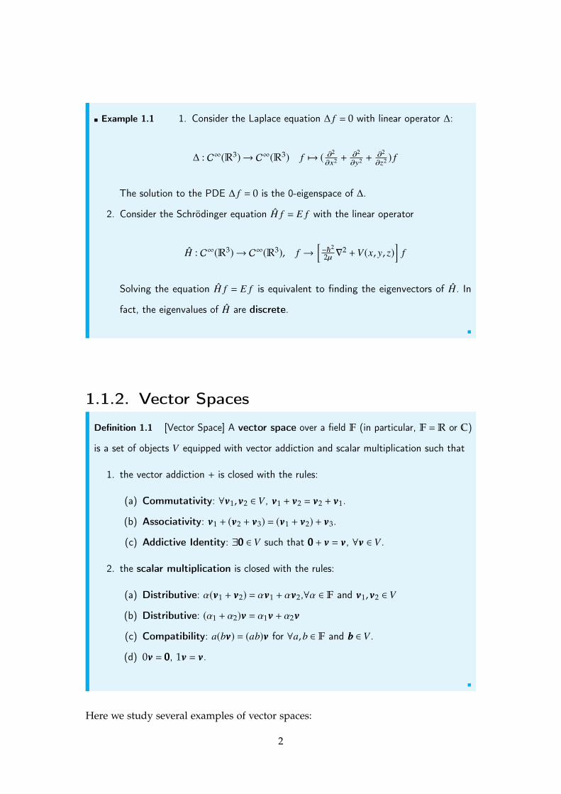
⌅ Example 1.1 1. Consider the Laplace equation � f = 0 with linear operator �:
� : C1(R3)! C1(R3) f 7! ( @2
@x2 +@2
@y2 +@2
@z2 ) f
The solution to the PDE � f = 0 is the 0-eigenspace of �.
2. Consider the Schrödinger equation H f = E f with the linear operator
H : C1(R3)! C1(R3), f !h�h2
2µ r2 +V(x, y, z)i
f
Solving the equation H f = E f is equivalent to finding the eigenvectors of H. In
fact, the eigenvalues of H are discrete.
⌅
1.1.2. Vector Spaces
Definition 1.1 [Vector Space] A vector space over a field F (in particular, F =R or C)
is a set of objects V equipped with vector addiction and scalar multiplication such that
1. the vector addiction + is closed with the rules:
(a) Commutativity: 8vvv1,vvv2 2 V , vvv1 + vvv2 = vvv2 + vvv1.
(b) Associativity: vvv1 + (vvv2 + vvv3) = (vvv1 + vvv2) + vvv3.
(c) Addictive Identity: 9000 2 V such that 000 + vvv = vvv, 8vvv 2 V .
2. the scalar multiplication is closed with the rules:
(a) Distributive: ↵(vvv1 + vvv2) = ↵vvv1 + ↵vvv2,8↵ 2 F and vvv1,vvv2 2 V
(b) Distributive: (↵1 + ↵2)vvv = ↵1vvv + ↵2vvv
(c) Compatibility: a(bvvv) = (ab)vvv for 8a, b 2 F and bbb 2 V .
(d) 0vvv = 000, 1vvv = vvv.
⌅
Here we study several examples of vector spaces:
2
⌅ Example 1.2 For V = Fn, we can define
1. Addictive Identity:
000 =
©≠≠≠≠≠´
0...
0
™ÆÆÆÆƨ
2. Scalar Multiplication:
↵
©≠≠≠≠≠´
x1...
xn
™ÆÆÆÆƨ=
©≠≠≠≠≠´
↵x1...
↵xn
™ÆÆÆÆƨ
3. Vector Addiction:©≠≠≠≠≠´
x1...
xn
™ÆÆÆÆƨ+
©≠≠≠≠≠´
y1...
yn
™ÆÆÆÆƨ=
©≠≠≠≠≠´
x1 + y1...
xn + yn
™ÆÆÆÆƨ
⌅
⌅ Example 1.3 1. It is clear that the set V = Mn⇥n(F) (the set of all m ⇥ n matrices)
is a vector space as well.
2. The set V = C(R) is a vector space:
(a) Vector Addiction:
( f + g)(x) = f (x) + g(x),8 f ,g 2 V
(b) Scalar Multiplication:
(↵ f )(x) = ↵ f (x),8↵ 2 R, f 2 V
(c) Addictive Identity is a zero function, i.e., 000(x) = 0 for all x 2 R.
⌅
3

Definition 1.2 A sub-collection W ✓ V of a vector space V is called a vector subspace
of V if W itself forms a vector space, denoted by W V . ⌅
⌅ Example 1.4 1. For V =R3, we claim that W = {(x, y,0) | x, y 2 R} V
2. W = {(x, y,1) | x, y 2 R} is not the vector subspace of V .
⌅
Proposition 1.1 W ✓ V is a vector subspace of V iff for 8www1,www2 2 W , we have ↵www1 +
�www2 2 W , for 8↵, � 2 F.
⌅ Example 1.5 1. For V = Mn⇥n(F), the subspace W = {A 2 V | AAAT = AAA} V
2. For V = C1(R), define W = { f 2 V | d2
dx2 f + f = 0} V . For f ,g 2 W , we have
(↵ f + �g)00 = ↵ f 00 + �g00 = ↵(� f ) + �(�g) = �(↵ f + �g),
which implies (↵ f + �g)00 + (↵ f + �g) = 0.
⌅
4

1.4. Wednesday for MAT3040
1.4.1. Review1. Vector Space: e.g., R, Mn⇥n(R),C(Rn),R[x].
2. Vector Subspace: W V , e.g.,
(a) V =R2, the set W :=R
2+ is not a vector subspace since W is not closed under
scalar multiplication;
(b) the set W = R2+
–R
2� is not a vector subspace since it is not closed under
addition.
(c) For V =M3⇥3(R), the set of invertible 3 ⇥ 3 matrices is not a vector subspace,
since we cannot define zero vector inside.
(d) Exercise: How about the set of all singular matrices? Answer: it is not a
vector subspace since the vector addition does not necessarily hold.
1.4.2. Spanning Set
Definition 1.11 [Span] Let V be a vector space over F:
1. A linear combination of a subset S in V is of the form
n’i=1
↵isssi, ↵i 2 F, sssi 2 S
Note that the summation should be finite.
2. The span of a subset S ✓ V is
span(S) =(
n’i=1
↵isssi
�����↵i 2 F, sssi 2 S
)
3. S is a spanning set of V , or say S spans V , if
span(S) = V .
14

⌅
⌅ Example 1.12 For V =R[x], define the set
S = {1, x2, x4, . . . , x6},
then 2 + x4 + ⇡x106 2 span(S), while the series 1 + x2 + x4 + · · · < span(S).
It is clear that span(S) ,V , but S is the spanning set of W = {p 2 V | p(x) = p(�x)}. ⌅
⌅ Example 1.13 For V =M3⇥3(R), let W1 = {AAA 2V | AAAT = AAA} and W2 = {BBB 2V | BBBT =�BBB}
(the set of skew-symmetric matrices) be two vector subspaces. Define the set
SSS :=W1
ÿW2
Exercise: SSS spans V . ⌅
Proposition 1.7 Let S be a subset in a vector space V .
1. S ✓ span(S)
2. span(S) = span(span(S))
3. If www 2 span{vvv1, . . . ,vvvn} \ span{vvv2, . . . ,vvvn}, then
vvv1 2 span{www,vvv2, . . . ,vvvn} \ span{vvv2, . . . ,vvvn}
Proof. 1. For each sss 2 S, we have
sss = 1 · sss 2 span(S)
2. From (1), it’s clear that span(S) ✓ span(span(S)), and therefore suffices to show
span(span(S)) ✓ span(S):
Pick vvv =Õn
i=1↵ivvvi 2 span(span(S)), where vvvi 2 span(S). Rewrite
vvvi =ni’j=1
�i j sss j , sss j 2 S,
15

which implies
vvv =n’i=1
↵i
ni’j=1
�i j sss j
=
n’i=1
ni’j=1
(↵i�i j)sss j ,
i.e., vvv is the finite combination of elements in S, whcih implies vvv 2 span(S).
3. By hypothesis, www = ↵1vvv1 + · · · + ↵nvvvn with ↵1 , 0, which implies
vvv1 = �↵2
↵1vvv2 + · · · +
✓� 1↵1
www
◆
which implies vvv1 2 span{www,vvv2, . . . ,vvvn}. It suffices to show vvv1 < span{vvv2, . . . ,vvvn}.
Suppose on the contrary that vvv1 2 span{vvv2, . . . ,vvvn}. It’s clear that span{vvv1, . . . ,vvvn} =
span{vvv2, . . . ,vvvn}. (left as exercise). Therefore,
; = span{vvv1, . . . ,vvvn} \ span{vvv2, . . . ,vvvn},
which is a contradiction.
⌅
1.4.3. Linear Independence and Basis
Definition 1.12 [Linear Independence] Let S be a (not necessarily finite) subset of V .
Then S is linearly independent (l.i.) on V if for any finite subset {sss1, . . . , sssk} in S,
k’i=1
↵isssi = 0 () ↵i = 0,8i
⌅
⌅ Example 1.14 For V = C(R),
16

1. let S1 = {sin x, cos x}, which is l.i., since
↵ sin x + �cos x = 000(means zero function)
Taking x = 0 both sides leads to � = 0; taking x = ⇡2 both sides leads to ↵ = 0.
2. let S2 = {sin2 x, cos2 x,1}, which is linearly dependent, since
1 · sin2 x + 1 · cos2 x + (�1) · 1 = 0,8x
3. Exercise: For V =R[x], let S = {1, x, x2, x3, . . . , }, which is l.i.:
Pick xk1 , . . . , xkn 2 S with k1 < · · · < kn. Consider that the euqation
↵1xk1 + · · · + ↵nxkn = 000
holds for all x, and try to solve for ↵1, . . . ,↵n (one way is differentation.)
⌅
Definition 1.13 [Basis] A subset S is a basis of V if
(a) S spans V ;
(b) S is l.i.
⌅
⌅ Example 1.15 1. For V =Rn, S = {eee1, . . . , eeen} is a basis of V
2. For V =R[x], S = {1, x, x2, . . . } is a basis of V
3. For V = M2⇥2(R),
S =
8>>><>>>:©≠≠´1 0
0 0
™Æƨ
,©≠≠´0 1
0 0
™Æƨ
,©≠≠´0 0
1 0
™Æƨ
,©≠≠´0 0
0 1
™Æƨ
9>>>=>>>;
is a basis of V
⌅
R Note that there can be many basis for a vector space V .
17
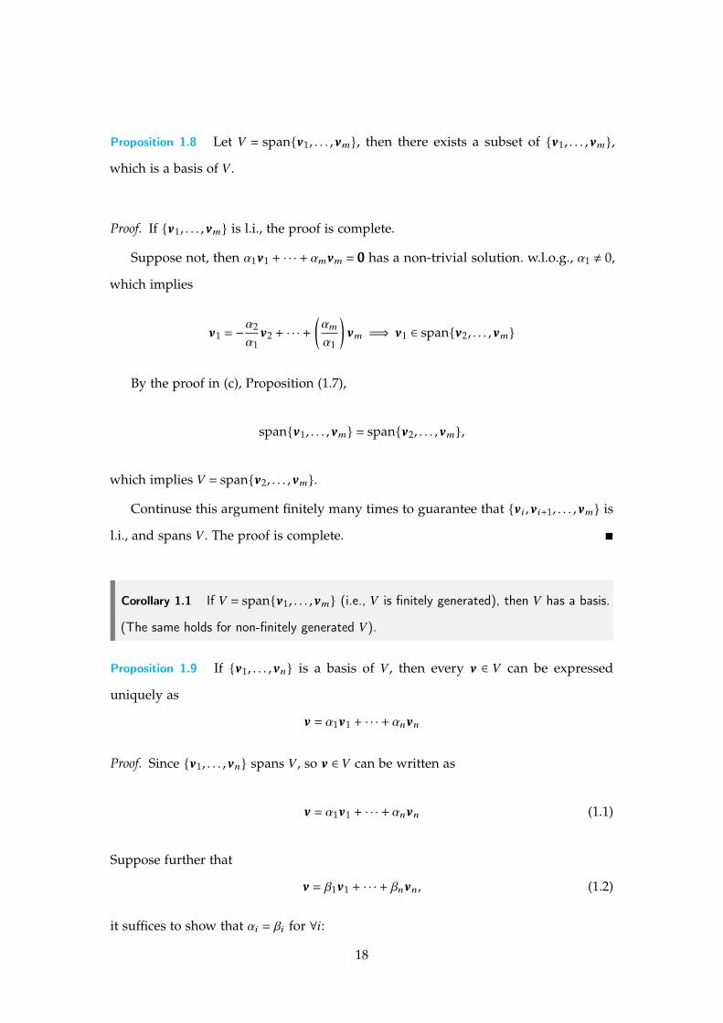
Proposition 1.8 Let V = span{vvv1, . . . ,vvvm}, then there exists a subset of {vvv1, . . . ,vvvm},
which is a basis of V .
Proof. If {vvv1, . . . ,vvvm} is l.i., the proof is complete.
Suppose not, then ↵1vvv1 + · · · + ↵mvvvm = 000 has a non-trivial solution. w.l.o.g., ↵1 , 0,
which implies
vvv1 = �↵2
↵1vvv2 + · · · +
✓↵m↵1
◆vvvm =) vvv1 2 span{vvv2, . . . ,vvvm}
By the proof in (c), Proposition (1.7),
span{vvv1, . . . ,vvvm} = span{vvv2, . . . ,vvvm},
which implies V = span{vvv2, . . . ,vvvm}.
Continuse this argument finitely many times to guarantee that {vvvi,vvvi+1, . . . ,vvvm} is
l.i., and spans V . The proof is complete. ⌅
Corollary 1.1 If V = span{vvv1, . . . ,vvvm} (i.e., V is finitely generated), then V has a basis.
(The same holds for non-finitely generated V).
Proposition 1.9 If {vvv1, . . . ,vvvn} is a basis of V , then every vvv 2 V can be expressed
uniquely as
vvv = ↵1vvv1 + · · · + ↵nvvvn
Proof. Since {vvv1, . . . ,vvvn} spans V , so vvv 2 V can be written as
vvv = ↵1vvv1 + · · · + ↵nvvvn (1.1)
Suppose further that
vvv = �1vvv1 + · · · + �nvvvn, (1.2)
it suffices to show that ↵i = �i for 8i:
18

Subtracting (1.1) into (1.2) leads to
(↵1 � �1)vvv1 + · · · + (↵n � �n)vvvn = 0.
By the hypothesis of linear independence, we have ↵i � �i = 0 for 8i, i.e., ↵i = �i. ⌅
19

Chapter 2
Week2
2.1. Monday for MAT3040Reviewing.
1. Linear Combination and Span
2. Linear Independence
3. Basis: a set of vectors {vvv1, . . . ,vvvk} is called a basis for V if {vvv1, . . . ,vvvk} is linearly
independent, and V = span{vvv1, . . . ,vvvk}.
Lemma: Given V = span{vvv1, . . . ,vvvk}, we can find a basis for this set. Here V is said
to be finitely generated.
4. Lemma: The vector www 2 span{vvv1, . . . ,vvvn} \ span{vvv2, . . . ,vvvn} implies that
vvv1 2 span{www,vvv2, . . . ,vvvn} \ span{vvv2, . . . ,vvvn}
2.1.1. Basis and DimensionTheorem 2.1 Let V be a finitely generated vector space. Suppose {vvv1, . . . ,vvvm} and
{www1, . . . ,wwwn} are two basis of V . Then m = n. (where m is called the dimension)
Proof. Suppose on the contrary that m , n. Without loss of generality (w.l.o.g.), assume
that m < n. Let vvv1 = ↵1www1 + · · ·+↵nwwwn, with some ↵i , 0. w.l.o.g., assume ↵1 , 0. Therefore,
vvv1 2 span{www1,www2, . . . ,wwwn} \ span{www2, . . . ,wwwn} (2.1)
which implies that www1 2 span{vvv1,www2, . . . ,wwwn} \ span{www2, . . . ,wwwn}.
33

Then we claim that {vvv1,www2, . . . ,wwwn} is a basis of V :
1. Note that {vvv1,www2, . . . ,wwwn} is a spannning set:
www1 2 span{vvv1,www2, . . . ,wwwn} =) {www1,www2, . . . ,wwwn} ✓ span{vvv1,www2, . . . ,wwwn}
=) span{www1,www2, . . . ,wwwn} ✓ span{span{vvv1,www2, . . . ,wwwn}} ✓ span{vvv1,www2, . . . ,wwwn}
Since V = span{www1,www2, . . . ,wwwn}, we have span{vvv1,www2, . . . ,wwwn} = V .
2. Then we show the linear independence of {vvv1,www2, . . . ,wwwn}. Consider the equation
�1vvv1 + �2vvv2 + · · · + �nwwwn = 000
(a) When �1 , 0, we imply
vvv1 =
✓� �2
�1
◆www2 + · · · +
✓� �n�1
◆wwwn 2 span{www2, . . . ,wwwn},
which contradicts (2.1).
(b) When �1 = 0, then �2www2 + · · · + �nwwwn = 000, which implies �2 = · · · = �n = 0, due
to the independence of {www2, . . . ,wwwn}.
Therefore, vvv2 2 span{vvv1,www2, . . . ,wwwn}, i.e.,
vvv2 = �1vvv1 + · · · + �nvvvn,
where �2, . . . ,�n cannot be all zeros, since otherwise {vvv1,vvv2} are linearly dependent, i.e.,
{vvv1, . . . ,vvvm} cannot form a basis. w.l.o.g., assume �2 , 0, which implies
www2 2 span{vvv1,vvv2,www3, . . . ,wwwn} \ span{vvv1,www3, . . . ,wwwn}.
Following the simlar argument above, {vvv1,vvv2,www3, . . . ,wwwn} forms a basis of V .
Continuing the argument above, we imply {vvv1, . . . ,vvvm,wwwm+1, . . . ,wwwn} is a basis of V .
34

Since {vvv1, . . . ,vvvm} is a basis as well, we imply
wwwm+1 = �1vvv1 + · · · + �mvvvm
for some �i 2 F, i.e., {vvv1, . . . ,vvvm,wwwm+1} is linearly dependent, which is a contradction. ⌅
⌅ Example 2.1 A vector space may have more than one basis.
Suppose V = Fn, it is clear that dim(V) = n, and
{eee1, . . . , eeen} is a basis of V , where eeei denotes a unit vector.
There could be other basis of V , such as
8>>>>>>>>><>>>>>>>>>:
©≠≠≠≠≠≠≠≠´
1
0...
0
™ÆÆÆÆÆÆÆƨ
,
©≠≠≠≠≠≠≠≠´
1
1...
0
™ÆÆÆÆÆÆÆƨ
, · · · ,
©≠≠≠≠≠≠≠≠´
1
1...
1
™ÆÆÆÆÆÆÆƨ
,
9>>>>>>>>>=>>>>>>>>>;
Actually, the columns of any invertible n ⇥ n matrix forms a basis of V . ⌅
⌅ Example 2.2 Suppose V = Mm⇥n(R), we claim that dim(V) = mn:
8>>><>>>:
Ei j
�������1 i m
1 j n
9>>>=>>>;
is a basis of V ,
where Ei j is m ⇥ n matrix with 1 at (i, j)-th entry, and 0s at the remaining entries. ⌅
⌅ Example 2.3 Suppose V = {all polynomials of degree n}, then dim(V) = n + 1. ⌅
⌅ Example 2.4 Supppose V = {AAA 2 Mn⇥n(R) | AAAT = AAA}, then dim(V) = n(n+1)2 . ⌅
⌅ Example 2.5 Let W = {BBB 2 Mn⇥n(R) | BBBT = �BBB}, then dim(V) = n(n�1)2 . ⌅
35

R Sometimes it should be classified the field F for the scalar multiplication to
define a vector space. Conside the example below:
1. Let V = C, then dim(C) = 1 for the scalar multiplication defined under
the field C.
2. Let V = span{1, i} = C, then dim(C) = 2 for the scalar multiplication
defined under the field R, since all z 2 V can be written as z = a + bi,
8a, b 2 R.
3. Therefore, to aviod confusion, it is safe to write
dimC(C) = 1, dimR(C) = 2.
2.1.2. Operations on a vector spaceNote that the basis for a vector space is characterized as the maximal linearly inde-
pendent set.
Theorem 2.2 — Basis Extension. Let V be a finite dimensional vector space, and
{vvv1, . . . ,vvvk} be a linearly independent set on V , Then we can extend it to the basis
{vvv1, . . . ,vvvk ,vvvk+1, . . . ,vvvn} of V .
Proof. • Suppose dim(V) = n > k, and {www1, . . . ,wwwn} is a basis of V . Consider the set
{www1, . . . ,wwwn}–{vvv1, . . . ,vvvk}, which is linearly dependent, i.e.,
↵1www1 + · · · + ↵nwwwn + �1vvv1 + · · · + �kvvvk = 000,
with some ↵i , 0, since otherwise this equation will only have trivial solution.
w.l.o.g., assume ↵1 , 0.
• Therefore, consider the set {www2, . . . ,wwwn}–{vvv1, . . . ,vvvk}. We keep removing elements
from {www2, . . . ,wwwn} until we first get the set
Sÿ
{vvv1, . . . ,vvvk},
36

with S ✓ {www1,www2, . . . ,wwwn} and S–{vvv1, . . . ,vvvk} is linearly independent, i.e., S is a
maximal subset of {www1, . . . ,wwwn} such that S–{vvv1, . . . ,vvvk} is linearly independent.
• Rewrite S = {vvvk+1, . . . ,vvvm} and therefore S0 = {vvv1, . . . ,vvvk ,vvvk+1, . . . ,vvvm} are linearly
independent. It suffices to show S0 spans V .
– Indeed, for all wwwi 2 {www1, . . . ,wwwn}, wwwi 2 span(S0), since otherwise the equation
↵wwwi + �1vvv1 + · · · + �mvvvm = 000 =) ↵ = 0,
which implies that �1vvv1 + · · · + �mvvvm = 000 admits only trivial solution, i.e.,
{wwwi}ÿ
S0 = {wwwi}ÿ
Sÿ
{vvv1, . . . ,vvvk} is linearly independent,
which violetes the maximality of S.
Therefore, all {www1, . . . ,wwwn} ✓ span(S0), which implies span(S0) = V .
Therefore, S0 is a basis of V .
⌅
R Start with a spanning set, we keep removing something to form a basis; start
with independent set, we keep adding something to form a basis.
In other words, the basis is both the minimal spanning set, and the maximal
linearly independent set.
Definition 2.1 [Direct Sum] Let W1,W2 be two vector subspaces of V , then
1. W1—
W2 := {www 2 V | www 2 W1, and www 2 W2}
2. W1 +W2 := {www1 + www2 | wwwi 2 Wi}
3. If furthermore that W1—
W2 = {000}, then W1 +W2 is denoted as W1 � W2, which is
called direct sum.
⌅
Proposition 2.1 W1—
W2 and W1 +W2 are vector subspaces of V .
37
2.4. Wednesday for MAT3040Reviewing.
• Basis, Dimension
• Basis Extension
• W1—
W2 = ; implies W1 � W2 =W1 +W2 (Direct Sum).
2.4.1. Remark on Direct Sum
Proposition 2.13 The set W1 +W2 = W1 � W2 iff any www 2 W1 +W2 can be uniquely
expressed as
www = www1 + www2,
where wwwi 2 Wi for i = 1,2.
R We can also define addiction among finite set of vector spaces {W1, . . . ,Wk}.
If www1 + · · · + wwwk = 000 implies wwwi = 0,8i, then we can write W1 + · · · +Wk as
W1 � · · · � Wk
Proposition 2.14 — Complementation. Let W V be a vector subspace of a fintie
dimension vector space V . Then there exists W 0 V such that
W � W 0 = V .
Proof. It’s clear that dim(W) := k n := dim(V). Suppose {vvv1, . . . ,vvvk} is a basis of W .
By the basis extension proposition, we can extend it into {vvv1, . . . ,vvvk ,vvvk+1, . . . ,vvvn},
which is a basis of V .
Therefore, we take W 0 = span{vvvk+1, . . . ,vvvn}, which follows that
51
1. W +W 0 = V : 8vvv 2 V has the form
vvv = (↵1vvv1 + · · · + ↵kvvvk) + (↵k+1vvvk+1 + · · · + ↵nvvvn) ,
where ↵1vvv1 + · · · + ↵kvvvk 2 W and ↵k+1vvvk+1 + · · · + ↵nvvvn 2 W 0.
2. W—
W 0 = {000}: Suppose vvv 2 W—
W 0, i.e.,
vvv = (�1vvv1 + · · · + �kvvvk) + (0vvvk+1 + · · · + 0vvvn) 2 W
= (0vvv1 + · · · + 0vvvk) + (�k+1vvvk+1 + · · · + �nvvvn) 2 W 0.
By the uniqueness of coordinates, we imply �1 = · · · = �n = 0, i.e., vvv = 000.
Therefore, we conclude that W � W 0 = V . ⌅
2.4.2. Linear TransformationDefinition 2.7 [Linear Transformation] Let V ,W be vector spaces. Then T : V ! W is a
linear transformation if
T(↵vvv1 + �vvv2) = ↵T(vvv1) + �T(vvv2),
for 8↵, � 2 F and vvv1,vvv2 2 V . ⌅
Proposition 2.15 1. Suppose that S : V ! W and T : W ! U are linear transforma-
tions, then so is T � S : V ! U.
2. For any linear transformation T : V ! W , we have
T(000V ) = 000W
Proof. Simply apply the definition of the linear transformation. ⌅
⌅ Example 2.12 1. The transformation T : Rn ! R
m defined as xxx 7! AAAxxx (where
AAA 2 Rm⇥n) is a linear transformation.
52
2. The transformation T : R[x]! R[x] defined as
p(x) 7! T(p(x)) = p0(x), p(x) 7! T(p(x)) =Ø x
0 p(t)dt
is a linear transformation
3. The transformation T : Mn⇥n(R)! R defined as
AAA 7! trace(AAA) :=n’i=1
aii
is a linear transformation.
However, the transformation
AAA 7! det(AAA)
is not a linear transformation.
⌅
Definition 2.8 [Kernel/Image] Let T : V ! W be a linear transfomation.
1. The kernel of T is
ker(T) = T�1(000) = {vvv 2 V | T(vvv) = 000}
2. The image (or range) of T is
Im(T) = T(vvv) = {T(vvv) 2 W | vvv 2 V}
⌅
⌅ Example 2.13 1. Let T : Rn ! R
n be a linear transformation with T(xxx) = AAAxxx, then
ker(T) = {xxx 2 Rn | AAAxxx = 000} = Null(AAA) Null Space
53

and
Im(T) = {AAAxxx | xxx 2 Rn} = Col(AAA) = span{columns of AAA} Column Space
2. For T(p(x)) = p0(x), ker(T) = {constant polynomials} and Im(T) =R[x].
⌅
Proposition 2.16 The kernel or image for a linear transformation T : V !W also forms
a vector subspace:
ker(T) V , Im(T) W
Proof. For vvv1,vvv2 2 ker(T), we imply
T(↵vvv1 + �vvv2) = 000,
which implies ↵vvv1 + �vvv2 2 ker(T).
The remaining proof follows similarly. ⌅
Definition 2.9 [Rank/Nullity] Let V ,W be finite dimensional vector spaces and T : V !W
a linear transformation. Then we define
rank(T) = dim(im(T))
nullity(T) = dim(ker(T))
⌅
R Let
HomF(V ,W) = {all linear transformations T : V ! W},
and we can define the addiction and scalar multiplication to make it a vector
space:
1. For T , S 2 HomF(V ,W), define
(T + S)(vvv) = T(vvv) + S(vvv),
54

which implies T + S 2 HomF(V ,W).
2. Also, define
(�T)(vvv) = �T(vvv), for 8� 2 F,
which implies �T 2 HomF(V ,W).
In particular, if V =Rn,W =R
m, then
HomF(V ,W) = Mm⇥n(R).
Proposition 2.17 If dim(V) = n,dim(W) = m, then dim(HomF(V ,W)) = mn.
Proposition 2.18 There are anternative characterizations for the injectivity and surjec-
tivity of lienar transformation T :
1. The linear transformation T is injective if and only if
ker(T) = 0,() nullity(T) = 0.
2. The linear transformation T is surjective if and only if
im(T) =W ,() rank(T) = dim(W).
3. If T is bijective, then T�1 is a linear transformation.
Proof. 1. (a) For the forward direction of (1),
xxx 2 ker(T) =) T(xxx) = 0 = T(000) =) xxx = 000
(b) For the reverse direction of (1),
T(xxx) = T(yyy) =) T(xxx � yyy) = 000 =) xxx � yyy 2 ker(T) = 000 =) xxx = yyy
2. The proof follows similar idea in (1).
3. Let T�1 : W ! V . For all www1,www2 2 W , there exists vvv1,vvv2 2 V such that T(vvvi) = wwwi , i.e.,
55

T�1(wwwi) = vvvi i = 1,2.
Consider the mapping
T(↵vvv1 + �vvv2) = ↵T(vvv1) + �T(vvv2)
= ↵www1 + �www2,
which implies ↵vvv1 + �vvv2 = T�1(↵www1 + �www2), i.e.,
↵T�1(www1) + �T�1(www2) = T�1(↵www1 + �www2).
⌅
Definition 2.10 [isomorphism] We say that the vector subspaces V and W are isomorphic
if there exists a bijective linear transfomation T : V ! W . (V �W)
This mapping T is called an isomorphism from V to W . ⌅
R If dim(V) = dim(W) = n <1, then V �W :
Take {vvv1, . . . ,vvvn}, {www1, . . . ,wwwn} as basis of V and W , respectively. Then one can
construct T : V ! W satisfying T(vvvi) = wwwi for 8i as follows:
T(↵1vvv1 + · · · + ↵nvvvn) = ↵nwww1 + · · · + ↵nwwwn 8↵i 2 F
It’s clear that our constructed T is a linear transformation.
R V �W doesn’t imply any linear transformations T : V !W is an isomorphism.
e.g., T(vvv) = 000 is not an isomorphic if W , {000}.
Theorem 2.3 — Rank-Nullity Theorem. Let T : V ! W be a linear transformation
with dim(V) <1. Then
rank(T) + nullity(T) = dim(V).
56
Proof. Since ker(T) V , by proposition (2.14), there exists V1 V such that
V = ker(T) � V1.
1. Consider the transformation T |V1 : V1 ! T(V1), which is an isomorphism, since:
• Surjectivity is immediate
• For vvv 2 ker(T |V1),
T(vvv) = 000 =) vvv 2 ker(T),
which implies vvv = 000 since vvv 2 ker(T)\V1 = 0, i.e., the injectivity follows.
Therefore, dim(V1) = dim(T(V1)).
2. Secondly, given an isomorphism T from X to Y with dim(X) <1, then dim(X) =
dim(T(X)). The reason follows from assignment 1 questions (8-9):
{vvv1, . . . ,vvvk} is a basis of X =) {T(vvv1), . . . ,T(vvvk)} is a basis of Y
3. Note that T(V1) = T(V) = im(T), since:
• for 8vvv 2 V , vvv = vvvk + vvv1, where vvvk 2 ker(T),vvv1 2 V1, which implies
T(vvv) = T(vvvk) +T(vvv1) = 000 +T(vvv1),
i.e., T(V) ✓ T(V1) ✓ T(V), i.e., T(V) = T(V1).
4. We can show that dim(V) = dim(ker(T)) + dim(V1): Let {v1, . . . ,vk} be a basis of
ker(T), and {vk+1, . . . ,vn} be a basis of V1, then by the proof of complementation
proposition (2.14), we imply {v1, . . . ,vn} is a basis of V , i.e., dim(V) = n = k + (n �
k) = dim(ker(T)) + dim(V1).
57

Therefore, we imply
dim(V) = dim(ker(T)) + dim(V1)
= nullity(T) + dim(T(V1))
= nullity(T) + dim(T(V))
= nullity(T) + dim(im(T))
= nullity(T) + rank(T).
⌅
58

Chapter 3
Week3
3.1. Monday for MAT3040Reviewing.
1. Complementation. Suppose dim(V) = n <1, then W V implies that there exists
W 0 such that
W � W 0 = V .
2. Given the linear transformation T : V ! W , define the set ker(T) and Im(T).
3. Isomorphism of vector spaces: T : V �W
4. Rank-Nullity Theorem
3.1.1. Remarks on IsomorphismProposition 3.1 If T : V ! W is an isomorphism, then
1. the set {vvv1, . . . ,vvvk} is linearly independent in V if and only if {Tvvv1, . . . ,Tvvvk} is
linearly independent.
2. The same goes if we replace the linearly independence by spans.
3. If dim(V) = n, then {vvv1, . . . ,vvvn} forms a basis of V if and only if {Tvvv1, . . . ,Tvvvn}
forms a basis of W . In particular, dim(V) = dim(W).
4. Two vector spaces with finite dimensions are isomorphic if and only if they have
the same dimension:
Proof. It suffices to show the reverse direction. Let {vvv1, . . . ,vvvn} and {www1, . . . ,wwwn} be two
73
basis of V ,W , respectively. Define the linear transformation T : V ! W by
T(a1vvv1 + · · · + anvvvn) = a1www1 + · · · + anwwwn
Then T is surjective since {www1, . . . ,wwwn} spans W ; T is injective since {www1, . . . ,wwwn} is
linearly independent. ⌅
3.1.2. Change of Basis and Matrix Representation
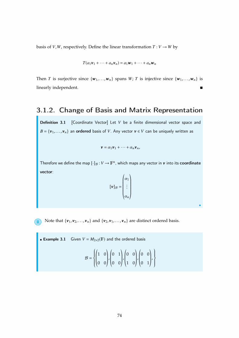
Definition 3.1 [Coordinate Vector] Let V be a finite dimensional vector space and
B = {vvv1, . . . ,vvvn} an ordered basis of V . Any vector vvv 2 V can be uniquely written as
vvv = ↵1vvv1 + · · · + ↵nvvvn,
Therefore we define the map [·]B : V ! Fn, which maps any vector in vvv into its coordinate
vector:
[vvv]B =©≠≠≠≠≠´
↵1...
↵n
™ÆÆÆÆƨ
⌅
R Note that {vvv1,vvv2, . . . ,vvvn} and {vvv2,vvv1, . . . ,vvvn} are distinct ordered basis.
⌅ Example 3.1 Given V = M2⇥2(F) and the ordered basis
B =8>>><>>>:©≠≠´1 0
0 0
™Æƨ
,©≠≠´0 1
0 0
™Æƨ
,©≠≠´0 0
1 0
™Æƨ
,©≠≠´0 0
0 1
™Æƨ
,
9>>>=>>>;
74

Any matrix has the coordinate vector w.r.t. B, i.e.,
2666664©≠≠´1 4
2 3
™Æƨ
3777775B=
©≠≠≠≠≠≠≠≠´
1
4
2
3
™ÆÆÆÆÆÆÆƨ
However, if given another ordered basis
B1 =
8>>><>>>:©≠≠´0 1
0 0
™Æƨ
,©≠≠´1 0
0 0
™Æƨ
,©≠≠´0 0
1 0
™Æƨ
,©≠≠´0 0
0 1
™Æƨ
,
9>>>=>>>;
,
the matrix may have the different coordinate vector w.r.t. B1:
2666664©≠≠´1 4
2 3
™Æƨ
3777775B1
=
©≠≠≠≠≠≠≠≠´
4
1
2
3
™ÆÆÆÆÆÆÆƨ
⌅
Theorem 3.1 The mapping [·]B : V ! Fn is an isomorphism.
Proof. 1. First show the operator [·]B is well-defined, i.e., the same input gives the
same output. Suppose that
[vvv]B =©≠≠≠≠≠´
↵1...
↵n
™ÆÆÆÆƨ
[vvv]B =©≠≠≠≠≠´
↵01...
↵0n
™ÆÆÆÆƨ
,
then we imply
vvv = ↵1vvv1 + · · · + ↵nvvvn
= ↵01vvv1 + · · · + ↵0
nvvvn.
75
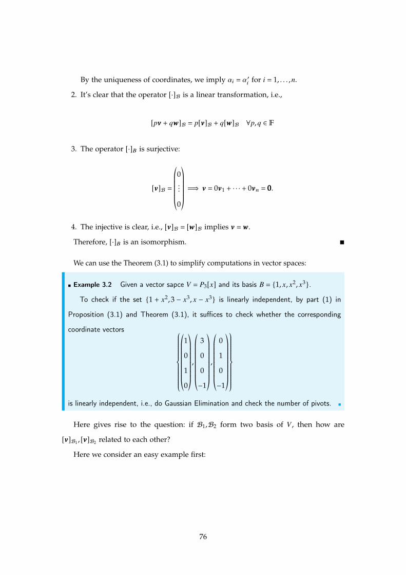
By the uniqueness of coordinates, we imply ↵i = ↵0i for i = 1, . . . ,n.
2. It’s clear that the operator [·]B is a linear transformation, i.e.,
[pvvv + qwww]B = p[vvv]B + q[www]B 8p, q 2 F
3. The operator [·]B is surjective:
[vvv]B =©≠≠≠≠≠´
0...
0
™ÆÆÆÆƨ=) vvv = 0vvv1 + · · · + 0vvvn = 000.
4. The injective is clear, i.e., [vvv]B = [www]B implies vvv = www.
Therefore, [·]B is an isomorphism. ⌅
We can use the Theorem (3.1) to simplify computations in vector spaces:
⌅ Example 3.2 Given a vector sapce V = P3[x] and its basis B = {1, x, x2, x3}.
To check if the set {1 + x2,3 � x3, x � x3} is linearly independent, by part (1) in
Proposition (3.1) and Theorem (3.1), it suffices to check whether the corresponding
coordinate vectors 8>>>>>>>>><>>>>>>>>>:
©≠≠≠≠≠≠≠≠´
1
0
1
0
™ÆÆÆÆÆÆÆƨ
,
©≠≠≠≠≠≠≠≠´
3
0
0
�1
™ÆÆÆÆÆÆÆƨ
,
©≠≠≠≠≠≠≠≠´
0
1
0
�1
™ÆÆÆÆÆÆÆƨ
9>>>>>>>>>=>>>>>>>>>;
is linearly independent, i.e., do Gaussian Elimination and check the number of pivots. ⌅
Here gives rise to the question: if B1,B2 form two basis of V , then how are
[vvv]B1 , [vvv]B2 related to each other?
Here we consider an easy example first:
76
⌅ Example 3.3 Consider V =Rn and its basis B1 = {eee1, . . . , eeen}. For any vvv 2 V ,
vvv =
©≠≠≠≠≠´
↵1...
↵n
™ÆÆÆÆƨ= ↵neee1 + · · · + ↵neeen =) [vvv]B1 =
©≠≠≠≠≠´
↵1...
↵n
™ÆÆÆÆƨ
Also, we can construct a different basis of V :
B2 =
8>>>>>>>>><>>>>>>>>>:
©≠≠≠≠≠≠≠≠´
1
0...
0
™ÆÆÆÆÆÆÆƨ
,
©≠≠≠≠≠≠≠≠´
1
1...
0
™ÆÆÆÆÆÆÆƨ
, . . . ,
©≠≠≠≠≠≠≠≠´
1
1...
1
™ÆÆÆÆÆÆÆƨ
9>>>>>>>>>=>>>>>>>>>;
,
which gives a different coordinate vector of vvv:
[vvv]B2 =
©≠≠≠≠≠≠≠≠≠≠≠≠´
↵1 � ↵2
↵2 � ↵3...
↵n�1 � ↵n↵n
™ÆÆÆÆÆÆÆÆÆÆÆƨ
⌅
Proposition 3.2 — Change of Basis. Let A = {vvv1, . . . ,vvvn} and A 0 = {www1, . . . ,wwwn} be two
ordered basis of a vector space V . Define the change of basis matrix from A to A 0, say
CA0,A := [↵i j], where
vvv j =m’i=1
↵i jwwwi
Then for any vector vvv 2 V , the change of basis amounts to left-multiplying the change of basis
matrix:
CA0,A[vvv]A = [vvv]A0 (3.1)
77

Define matrix CA,A0 := [�i j], where
www j =
n’i=1
�i jvvvi
Then we imply that
(CA,A0)�1 = CA0,A
Proof. 1. First show (3.1) holds for vvv = vvv j , j = 1, . . . ,n:
LHS of (3.1) = [↵i j]eee j =
©≠≠≠≠≠´
↵1j...
↵nj
™ÆÆÆÆƨ
RHS of (3.1) = [vvv j]A0 =
"n’i=1
↵iwwwi
#A0
=
©≠≠≠≠≠´
↵1j...
↵nj
™ÆÆÆÆƨ
Therefore,
CA0,A[vvv j]A = [vvv j]A0, 8 j = 1, . . . ,n. (3.2)
2. Then for any vvv 2 V , we imply vvv = r1vvv1 + · · · + rnvvvn, which implies that
CA0,A[vvv]A = CA0,A[r1vvv1 + · · · + rnvvvn]A (3.3a)
= CA0,A (r1[vvv1]A + · · · + rn[vvvn]A) (3.3b)
=
n’j=1
rjCA0,A[vvv j]A (3.3c)
=
n’j=1
rj[vvv j]A0 (3.3d)
=
266664n’j=1
rjvvv j
377775A0
(3.3e)
= [vvv]A0 (3.3f)
where (3.3a) and (3.3e) is by applying the lineaity of [·]A and [·]A0; (3.3d) is by
applying the result (3.12). Therefore (3.1) is shown for 8vvv 2 V .
78
3. Now we show that (CAA0CA0A) = IIIn. Note that
vvv j =n’i=1
↵i jwwwi
=
n’i=1
↵i j
n’k=1
�kivvvk
=
n’k=1
n’i=1
�ki↵i j
!vvvi
By the uniqueness of coordinates, we imply
n’i=1
�ki↵i j
!= �jk :=
8>>><>>>:
1, j = k
0, j , k
By the matrix multiplication, the (k, j)-th entry for CAA0CA0A is
[CAA0CA0A]k j =
n’i=1
�ki↵i j
!= �jk =) (CAA0CA0A) = IIIn
Noew, suppose
vvv j =n’i=1
↵i jwwwi
=
n’i=1
↵i j
n’k=1
�kivvvk
=
n’k=1
n’i=1
�ki↵i j
!vvvi
By the uniqueness of coordinates, we imply
n’i=1
�ki↵i j
!=
8>>><>>>:
1, j = k
0, j , k
where n’i=1
�ki↵i j
!= (CAA0CA0A) .
Therefore, (CAA0CA0A) = IIIn. ⌅
79

⌅ Example 3.4 Back to Example (3.3), write B1,B2 as
B1 = {eee1, . . . , eeen}, B2 = {www1, . . . ,wwwn}
and therefore wwwi = eee1 + · · · + eeei. The change of basis matrix is given by
CB1,B2 =
©≠≠≠≠≠≠≠≠´
1 1 · · · 1
0 1 · · · 1...
... . . . ...
0 0 · · · 1
™ÆÆÆÆÆÆÆƨ
which implies that for vvv in the example,
CB1,B2[vvv]B2 =
©≠≠≠≠≠≠≠≠´
1 1 · · · 1
0 1 · · · 1...
... . . . ...
0 0 · · · 1
™ÆÆÆÆÆÆÆƨ
©≠≠≠≠≠≠≠≠´
↵1 � ↵2...
↵n�1 � ↵n↵n
™ÆÆÆÆÆÆÆƨ
=
©≠≠≠≠≠´
↵1...
↵n
™ÆÆÆÆƨ= [vvv]B1
⌅
Definition 3.2 Let T : V ! W be a linear transformation, and
A = {vvv1, . . . ,vvvm}, B = {www1, . . . ,wwwm}
be basis of V and W , respectively. The matrix representation of T with respect to (w.r.t.)
A and B is defined as (T)BA := (↵i j) 2 Mm⇥m(F), where
T(vvv j) =m’i=1
↵i jwwwi
⌅
80

3.4. Wednesday for MAT3040
3.4.1. Remarks for the Change of BasisReviewing.
• [·]A : V ! Fn denotes coordinate vector mapping
• Change of Basis matrix: CA0,A
• T : V ! W , A = {vvv1, . . . ,vvvn} and BBB = {www1, . . . ,wwwm}.
HomF(V ,W)! Mm⇥n(F)
⌅ Example 3.10 Let V = P3[x] and A = {1, x, x2, x3}.
Let T : V ! V defined as p(x) 7! p0(x):
8>>>>>>>>>><>>>>>>>>>>:
T(1) = 0 · 1 + 0 · x + 0 · x2 + 0 · x3
T(x) = 1 · 1 + 0 · x + 0 · x2 + 0 · x3
T(x2) = 0 · 1 + 2 · x + 0 · x2 + 0 · x3
T(x3) = 0 · 1 + 0 · x + 3 · x2 + 0 · x3
We can define the change of basis matrix for a linear transformation T as well, w.r.t.
A and A:
CA,A =
©≠≠≠≠≠≠≠≠´
0 1 0 0
0 0 2 0
0 0 0 3
0 0 0 0
™ÆÆÆÆÆÆÆƨ
Also, we can define a different basis A 0 = {x3, x2, x, 1} for the output space for T , say
T : VA ! VA0:
(T)A,A0 =
©≠≠≠≠≠≠≠≠´
0 0 0 0
0 0 0 3
0 0 2 0
0 1 0 0
™ÆÆÆÆÆÆÆƨ
92

Our observation is that the corresponding coordinate vectors before and after linear
transformation admits a matrix multiplication:
(2x2 + 4x3) T�! ((4x + 12x2))
(2x2 + 4x3)A =
©≠≠≠≠≠≠≠≠´
0
0
2
4
™ÆÆÆÆÆÆÆƨ
(4x + 12x2)A =
©≠≠≠≠≠≠≠≠´
0
4
12
0
™ÆÆÆÆÆÆÆƨ
©≠≠≠≠≠≠≠≠´
0 1 0 0
0 0 2 0
0 0 0 3
0 0 0 0
™ÆÆÆÆÆÆÆƨ
©≠≠≠≠≠≠≠≠´
0
0
2
4
™ÆÆÆÆÆÆÆƨ
=
©≠≠≠≠≠≠≠≠´
0
4
12
0
™ÆÆÆÆÆÆÆƨ
CAA · (2x2 + 4x3)A = (4x + 12x2)A
⌅
Theorem 3.3 — Matrix Representation. Let T : V ! W be a linear transformation of
finite dimensional vector sapces. Let A,B the ordered basis of V ,W , respectively.
Then the following diagram holds:
Figure 3.2: Diagram for the matrix reprentation, where n := dim(V) and m := dim(W)
93

namely, for any vvv 2 V ,
(T)B,A(vvv)A = (Tvvv)B
Therefore, we can compute Tvvv by matrix multiplication.
Therefore, linear transformation corresponds to coordinate matrix multiplication.
Proof. Suppose A = {vvv1, . . . ,vvvn} and B = {www1, . . . ,wwwn}. The proof of this theorem follows
the same procedure of that in Theorem (3.1)
1. We show this result for vvv = vvv j first:
LHS = [↵i j]eee j =
©≠≠≠≠≠´
↵1j...
↵nj
™ÆÆÆÆƨ
RHS = (Tvvv j)B =
m’i=1
↵i jwwwi
!B=
©≠≠≠≠≠´
↵1j...
↵nj
™ÆÆÆÆƨ
2. Then we show the theorem holds for any vvv :=Õn
j=1 rjvvv j in V :
(T)BA(vvv)A = (T)BA©≠´
n’j=1
rjvvv j™Æ¨A
(3.8a)
= (T)BA©≠´
n’j=1
rj(vvv j)A™Æ¨
(3.8b)
=
n’j=1
rj(T)BA(vvv j)A (3.8c)
=
n’j=1
rj(Tvvv j)B (3.8d)
=©≠´
n’j=1
rj(Tvvv j)™Æ¨B
(3.8e)
=
266664T(
n’j=1
rjvvv j)377775B
(3.8f)
= (Tvvv)B (3.8g)
94

The justification for (3.8a) is similar to that shown in Theorem (3.1). The proof is
complete.
⌅
R Consider a special case for Theorem (3.3), i.e., T = id and A,A 0 are two
ordered basis for the input and output space, respectively. Then the result in
Theorem (3.3) implies
CA0,A(vvv)A = (vvv)A0
i.e., the matrix representation theorem (3.3) is a general case for the change
of basis theorem (3.1)
Proposition 3.6 — Functoriality. Suppose V ,W ,U are finite dimensional vector spaces,
and let A,B,C be the ordered basis for V ,W ,U, respectively. Suppose that
T : V ! W , S : W ! U
are given two linear transformations, then
(S �T)C,A = (S)C,B(T)B,A
Composition of linear transformation corresponds to the multiplication of change
of basis matrices.
Proof. Suppose the ordered basis A = {vvv1, . . . ,vvvn}, B = {www1, . . . ,wwwm}, C = {uuu1, . . . ,uuup}. By
defintion of change of basis matrices,
T(vvv j) =’i
(TB,A)i jwwwi
S(wwwi) =’k
(SC,B)kiuuuk
95
We start from the j-th column of (S �T)C,A for j = 1, . . . ,n, namely
(S �T)C,A(vvv j)A = (S �T(vvv j))C (3.9a)
=
"S �
’i
(TB,A)i jwwwi
!#C
(3.9b)
=’i
(TB,A)i j (S(wwwi))C (3.9c)
=’i
(TB,A)i j ’
k
(SC,B)kiuuuk
!C
(3.9d)
=’k
’i
(SC,B)ki(TB,A)i j(uuuk)C (3.9e)
=’k
(SC,BTB,A)k j(uuuk)C (3.9f)
=’k
(SC,BTB,A)k jeeek (3.9g)
= j-th column of [SCBTB,A] (3.9h)
where (3.9a) is by the result in theorem (3.3); (3.9b) and (3.9d) follows from definitions
of T(vvv j) and S(wwwi); (3.9c) and (3.9e) follows from the linearity of C; (3.9f) follows from
the matrix multiplication definition; (3.9g) is because (uuuk)C = eeek .
Therefore, (S �T)CA and (SC,B)(TB,A) share the same j-th column, and thus equal
to each other. ⌅
Corollary 3.2 Suppose that S and T are two identity mappings V ! V , and consider
(S)A0A and (T)A,A0 in proposition (3.6), then
(S �T)A0,A0 = (S)A0A(T)A,A0
Therefore,
Identity matrix = CA0,ACA,A0
Proposition 3.7 Let T : V ! W with dim(V) = n,dim(W) = m, and let
• A,A 0 be ordered basis of V
96
• B,B 0 be ordered basis of W
then the change of basis matrices admit the relation
(T)B0,A0 = CB0,B(T)B,ACAA0 (3.10)
Here note that (T)B0,A0, (T)B,A 2 Fm⇥n; CB0,B 2 F
m⇥m; and CAA0 2 Fn⇥n.
Proof. Let A = {vvv1, . . . ,vvvn},A 0 = {vvv01, . . . ,vvv0n}. Consider simplifying the j-th column for
the LHS and RHS of (3.10) and showing they are equal:
LHS = (T)B0,A0eee j
= (T)B0,A0(vvv0j)A0
= (Tvvv0j)B0
RHS = CB0,B(T)B,ACAA0eee j
= CB0,B(T)B,ACAA0(vvv0j)A0
= CB0,B(T)B,A(vvv0j)A
= CB0,B(Tvvv0j)B
= (Tvvv0j)B0
⌅
R Let T : V ! V be a linear operator with A,A 0 being two ordered basisof V ,
then
(T)A0A0 = CA0,A(T)AACA,A0 = (CA,A0)�1(T)AACA,A0
Therefore, the change of basis matrices (T)A0A0 and (T)AA are similar to each
other, which means they share the same eigenvalues, determinant, trace.
Therefore, two similar matrices cooresponds to same linear transformation
using different basis.
97

Chapter 4
Week4
4.1. Monday for MAT3040
4.1.1. Quotient Spaces
Now we aim to divide a big vector space into many pieces of slices.
• For example, the Cartesian plane can be expressed as union of set of vertical lines
as follows:
R2 =
ÿm2R
8>>><>>>:©≠≠´m
0
™Æƨ+ span{(0,1)}}
9>>>=>>>;
• Another example is that the set of integers can be expressed as union of three
sets:
Z = Z1 [ Z2 [ Z3,
where Zi is the set of integers z such that z mod 3 = i.
Definition 4.1 [Coset] Let V be a vector space and W V . For any element vvv 2 V , the
(right) coset determined by vvv is the set
vvv +W := {vvv + www | www 2 W}
⌅
For example, consider V =R3 and W = span{(1,2,0)}. Then the coset determined by
109

vvv = (5,6,�3) can be written as
vvv +W = {(5 + t,6 + 2t,�3) | t 2 R}
It’s interesting that the coset determined by vvv0 = {(4,4,�3)} is exactly the same as the
coset shown above:
vvv0 +W = {(4 + t,4 + 2t,�3) | t 2 R} = vvv +W .
Therefore, write the exact expression of vvv +W may sometimes become tedious and
hard to check the equivalence. We say vvv is a representative of a coset vvv +W .
Proposition 4.1 Two cosets are the same iff the subtraction for the corresponding
representatives is in W , i.e.,
vvv1 +W = vvv2 +W () vvv1 � vvv2 2 W
Proof. Necessity. Suppose that vvv1+W = vvv2+W , then vvv1+www1 = vvv2+www2 for some www1,www2 2W ,
which implies
vvv1 � vvv2 = www2 � www1 2 W
Sufficiency. Suppose that vvv1 � vvv2 = www 2 W . It suffices to show vvv1 +W ✓ vvv2 +W . For any
vvv1 + www0 2 vvv1 +W , this element can be expressed as
vvv1 + www0 = (vvv2 + www) + www0 = vvv2 + (www + www0)| {z }
belong to W
2 vvv2 +W .
Therefore, vvv1 +W ✓ vvv2 +W . Similarly we can show that vvv2 +W ✓ vvv1 +W . ⌅
Exercise: Two cosets with representatives vvv1,vvv2 have no intersection iff vvv1 � vvv2 <W .
Definition 4.2 [Quotient Space] The quotient space of V by the subspace W , is the
collection of all cosets vvv +W , denoted by V/W . ⌅
To make the quotient space a vector space structure, we define the addition and scalar
110

multiplication on V/W by:
(vvv1 +W) + (vvv2 +W) := (vvv1 + vvv2) +W
↵ · (vvv +W) := (↵ · vvv) +W
For example, consider V =R2 and W = span{(0,1)}. Then note that
©≠≠´©≠≠´1
0
™Æƨ+W
™Æƨ+
©≠≠´©≠≠´2
0
™Æƨ+W
™Æƨ=
©≠≠´©≠≠´3
0
™Æƨ+W
™Æƨ
⇡ ·©≠≠´©≠≠´1
0
™Æƨ+W
™Æƨ=
©≠≠´©≠≠´⇡
0
™Æƨ+W
™Æƨ
Proposition 4.2 The addition and scalar multiplication is well-defined.
Proof. 1. Suppose that 8>>><>>>:vvv1 +W = vvv01 +W
vvv2 +W = vvv02 +W, (4.1)
and we need to show that (vvv1 + vvv2) +W = (vvv01 + vvv02) +W .
From (4.1) and proposition (4.1), we imply
vvv1 � vvv01 2 W , vvv2 � vvv02 2 W
which implies
(vvv1 � vvv01) + (vvv2 � vvv02) = (vvv1 + vvv2) � (vvv01 + vvv02) 2 W
By proposition (4.1) again we imply (vvv1 + vvv2) +W = (vvv01 + vvv02) +W
2. For scalar multiplication, similarly, we can show that vvv1 +W = vvv01 +W implies
↵vvv1 +W = ↵vvv01 +W for all ↵ 2 F.
⌅
111

Proposition 4.3 The canonical projection mapping
⇡W :V ! V/W ,
vvv 7! vvv +W ,
is a surjective linear transformation with ker(⇡W ) =W .
Proof. 1. First we show that ker(⇡W ) =W :
⇡W (vvv) = 0 =) vvv +W = 000V/W =) vvv +W = 000 +W =) vvv = (vvv � 000) 2 W
Here note that the zero element in the quotient space V/W is the coset with
representative 000.
2. For any vvv0+W 2V/W , we can construct vvv0 2V such that ⇡W (vvv0)= vvv0+W . Therefore
the mapping ⇡W is surjective.
3. To show the mapping ⇡W is a linear transformation, note that
⇡W (↵vvv1 + �vvv2) = (↵vvv1 + �vvv2) +W
= (↵vvv1 +W) + (�vvv2 +W)
= ↵(vvv1 +W) + �(vvv2 +W)
= ↵⇡W (vvv1) + �⇡W (vvv2)
⌅
4.1.2. First Isomorphism Theorem
The key of linear algebra is to solve the linear system AAAxxx = bbb with AAA 2 Rm⇥n. The
general step for solving this linear system is as follows:
1. Find the solution set for AAAxxx = 000, i.e., the set ker(AAA)
2. Find a particular solution xxx0 such that AAAxxx0 = bbb.
Then the general solution set to this linear system is xxx0 + ker(AAA), which is a coset in
112
the space Rn/ker(AAA). Therefore, to solve the linear system AAAxxx = bbb suffices to study the
quotient space Rn/ker(AAA):
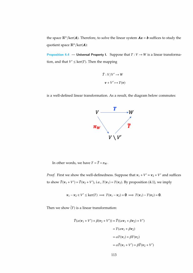
Proposition 4.4 — Universal Property I. Suppose that T : V ! W is a linear transforma-
tion, and that V 0 ker(T). Then the mapping
T : V/V 0 ! W
vvv +V 0 7! T(vvv)
is a well-defined linear transformation. As a result, the diagram below commutes:
In other words, we have T = T � ⇡W .
Proof. First we show the well-definedness. Suppose that vvv1 +V 0 = vvv2 +V 0 and suffices
to show T(vvv1 +V 0) = T(vvv2 +V 0), i.e., T(vvv1) = T(vvv2). By proposition (4.1), we imply
vvv1 � vvv2 2 V 0 ker(T) =) T(vvv1 � vvv2) = 000 =) T(vvv1) �T(vvv2) = 000.
Then we show (T) is a linear transformation:
T(↵(vvv1 +V 0) + �(vvv2 +V 0)) = T((↵vvv1 + �vvv2) +V 0)
= T(↵vvv1 + �vvv2)
= ↵T(vvv1) + �T(vvv2)
= ↵T(vvv1 +V 0) + �T(vvv2 +V 0)
113
⌅
Actually, if we let V 0 = ker(T), the mapping T : V/V 0 ! T(V) forms an isomorphism,
In particular, if further T is surjective, then T(V) =W , i.e., the mapping T : V/V 0 ! W
forms an isomorphism.
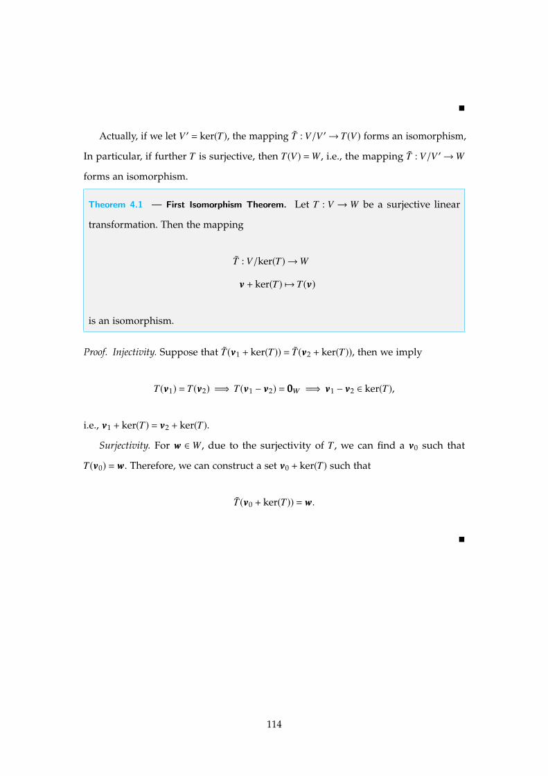
Theorem 4.1 — First Isomorphism Theorem. Let T : V ! W be a surjective linear
transformation. Then the mapping
T : V/ker(T)! W
vvv + ker(T) 7! T(vvv)
is an isomorphism.
Proof. Injectivity. Suppose that T(vvv1 + ker(T)) = T(vvv2 + ker(T)), then we imply
T(vvv1) = T(vvv2) =) T(vvv1 � vvv2) = 000W =) vvv1 � vvv2 2 ker(T),
i.e., vvv1 + ker(T) = vvv2 + ker(T).
Surjectivity. For www 2 W , due to the surjectivity of T , we can find a vvv0 such that
T(vvv0) = www. Therefore, we can construct a set vvv0 + ker(T) such that
T(vvv0 + ker(T)) = www.
⌅
114
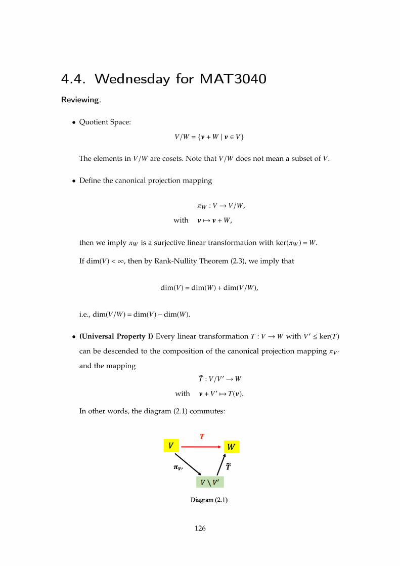
4.4. Wednesday for MAT3040Reviewing.
• Quotient Space:
V/W = {vvv +W | vvv 2 V}
The elements in V/W are cosets. Note that V/W does not mean a subset of V .
• Define the canonical projection mapping
⇡W : V ! V/W ,
with vvv 7! vvv +W ,
then we imply ⇡W is a surjective linear transformation with ker(⇡W ) =W .
If dim(V) <1, then by Rank-Nullity Theorem (2.3), we imply that
dim(V) = dim(W) + dim(V/W),
i.e., dim(V/W) = dim(V) � dim(W).
• (Universal Property I) Every linear transformation T : V ! W with V 0 ker(T)
can be descended to the composition of the canonical projection mapping ⇡V 0
and the mapping
T : V/V 0 ! W
with vvv +V 0 7! T(vvv).
In other words, the diagram (2.1) commutes:
126
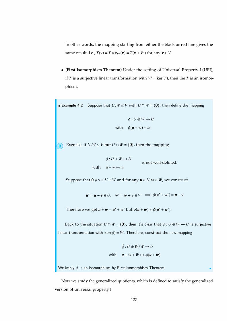
In other words, the mapping starting from either the black or red line gives the
same result, i.e., T(vvv) = T � ⇡V 0(vvv) = T(vvv +V 0) for any vvv 2 V .
• (First Isomorphism Theorem) Under the setting of Universal Property I (UPI),
if T is a surjective linear transformation with V 0 = ker(T), then the T is an isomor-
phism.
⌅ Example 4.2 Suppose that U,W V with U \W = {000}, then define the mapping
� : U � W ! U
with �(uuu + www) = uuu
R Exercise: if U,W V but U \W , {000}, then the mapping
� : U +W ! U
with uuu + www 7! uuuis not well-defined:
Suppose that 000 , vvv 2 U \W and for any uuu 2 U,www 2 W , we construct
uuu0 = uuu � vvv 2 U, www0 = www + vvv 2 V =) �(uuu0 + www0) = uuu � vvv
Therefore we get uuu + www = uuu0 + www0 but �(uuu + www) , �(uuu0 + www0).
Back to the situation U \W = {000}, then it’s clear that � : U � W ! U is surjective
linear transformation with ker(�) =W . Therefore, construct the new mapping
� : U � W/W ! U
with uuu + www +W 7! �(uuu + www)
We imply � is an isomorphism by First Isomorphism Theorem. ⌅
Now we study the generalized quotients, which is defined to satisfy the generalized
version of universal property I.
127

Definition 4.7 [Universal Property for Quotients] Let V be a vector space and V 0 V .
Consider the collection of linear transformations
Obj =
8>>><>>>:
T : V ! W
�������T is a linear transformation
V 0 ker(T)
9>>>=>>>;
(For example, ⇡V 0 : V ! V/V 0 is an element from the set Obj.)
An element (� : V ! U) 2 Obj is said to satisfy the universal property if it satisfies
the following:
Given any element (T : V ! W) 2 Obj, we can extend the transformation
� with a uniquely existing T : U ! W so that the diagram (2.2) commutes:
Or equivalently, for given (T : V ! W) 2 Obj, there exists the unique
mapping T : U ! W such that T = T � �.
⌅
Theorem 4.3 — Universal Property II. 1. The mapping (⇡V 0 : V ! V/V 0) 2 Obj is
a universal object, i.e., it satisfies the universal property.
2. If (� : V !U) is a universal object, then U � V/V 0, i.e., there is intrinsically “one”
element in the set of universal objects.
Proof. 1. Consider any linear transformation T : V ! W such that V 0 ker(T), then
define (construct) the same T : V/V 0 ! W as that in UPI. Therefore, for given T ,
applying the result of UPI, we imply T = T � ⇡V 0 , i.e., ⇡V 0 satisfies the diagram (2.2).
128
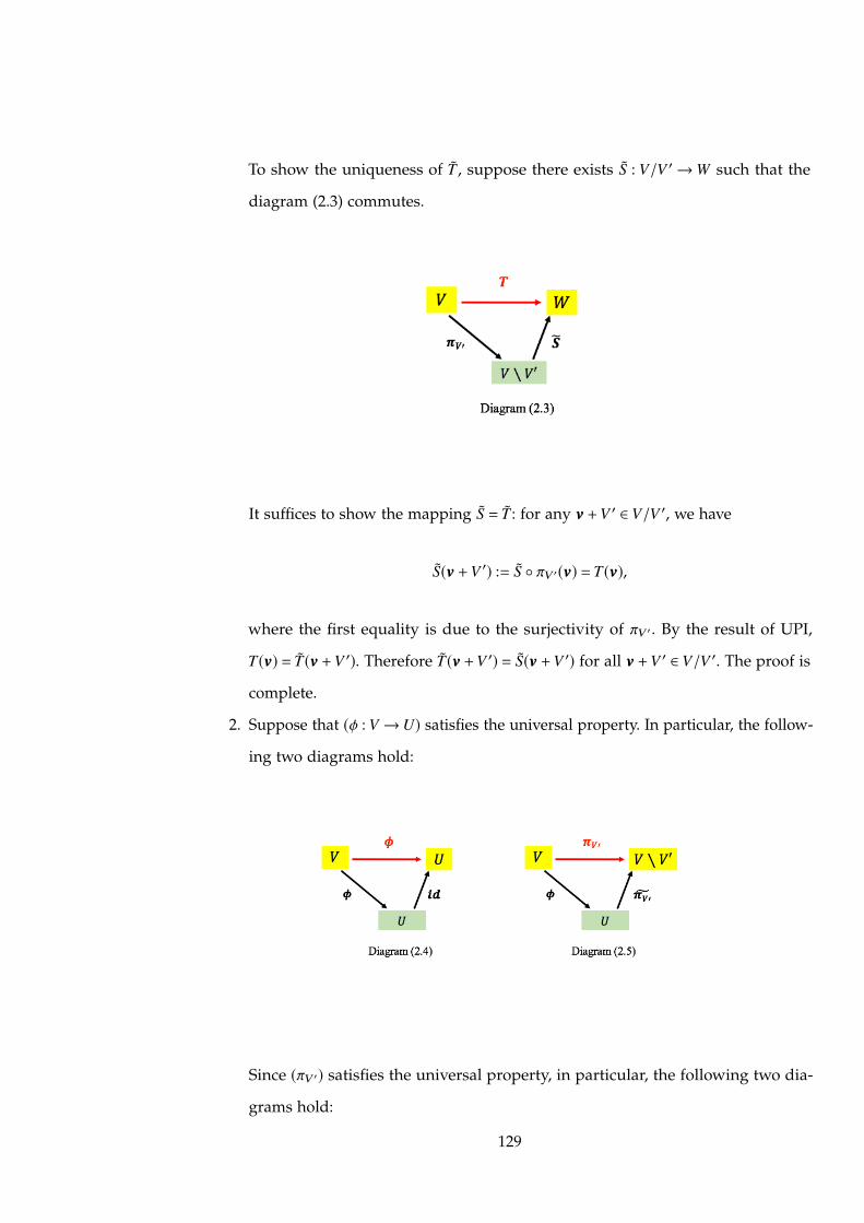
To show the uniqueness of T , suppose there exists S : V/V 0 ! W such that the
diagram (2.3) commutes.
It suffices to show the mapping S = T : for any vvv +V 0 2 V/V 0, we have
S(vvv +V 0) := S � ⇡V 0(vvv) = T(vvv),
where the first equality is due to the surjectivity of ⇡V 0. By the result of UPI,
T(vvv) = T(vvv +V 0). Therefore T(vvv +V 0) = S(vvv +V 0) for all vvv +V 0 2 V/V 0. The proof is
complete.
2. Suppose that (� : V ! U) satisfies the universal property. In particular, the follow-
ing two diagrams hold:
Since (⇡V 0) satisfies the universal property, in particular, the following two dia-
grams hold:
129

Then we claim that: Combining Diagram (2.5) and (2.6), we imply the dia-
gram (2.8):
Graph Description: Note that this diagram commutes, i.e., the mapping startingfrom either the red line or the dash line gives the same result, i.e., ⇡V 0 = ⇡V 0 � � � ⇡V 0.Comparing Diagram (2.7) and Diagram (2.8), we have ⇡V 0 � � = id, by the uniqueness
of the universal object.
Therefore, ⇡V 0 � � = id implies ⇡V 0 is surjective and � is injective.
Also, combining Diagram (2.6) and (2.5), we imply diagram (2.9):
130

Graph Description: Note that this diagram commutes, i.e., the mapping starting fromeither the red line or the dash line gives the same result, i.e., � = � � ⇡V 0 � �. ComparingDiagram (2.9) and Diagram (2.4), we have � � ⇡V 0 = id, by the uniqueness of theuniversal object
Therefore, � � ⇡V 0 = id implies � is surjective and ⇡V 0 is injective.
Therefore, both � : U ! V/V 0 and ⇡V 0 : V/V 0 ! U are bijective, i.e., U � V/V 0. The
proof is complete.
⌅
4.4.1. Dual Space
Definition 4.8 Let V be a vector space over a field F. The dual vector space V⇤ is
defined as
V⇤ = HomF(V ,F)
= { f : V ! F | f is a linear transformation}
⌅
131

⌅ Example 4.3 1. Consider V =Rn and define �i : V ! R as the i-th component of
input:
�i
©≠≠≠≠≠´
x1...
xn
™ÆÆÆÆƨ= xi,
Then we imply �i 2 V⇤. On the contrary, �2i
©≠≠≠≠≠´
x1...
xn
™ÆÆÆÆƨ= x2
i is not in V⇤
2. Consider V = F[x] and define � : V ! F as:
�(p(x)) = p(1),
It’s clear that � 2 V⇤:
�(ap(x) + bq(x)) = ap(1) + bq(1)
= a�(p(x)) + b�(q(x))
3. Also, : V ! F by (p(x)) =Ø 1
0 p(x)dx is in V⇤.
4. Also, for V =Mn⇥n(F), the mapping tr : V !F by tr(M)=Õni=1 Mii is in V⇤. However,
the det : V ! F is not in V⇤
⌅
Definition 4.9 Let V be a vector space, with basis B = {vi | i 2 I} (I can be finite or
countable, or uncountable). Define
B⇤ = { fi : V ! F | i 2 I},
132
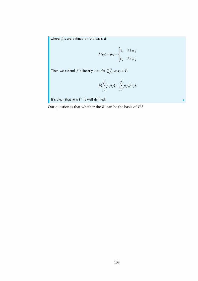
where fi’s are defined on the basis B:
fi(vj) = �i j =8>>><>>>:
1, if i = j
0, if i , j
Then we extend fi’s linearly, i.e., forÕN
j=1↵jvj 2 V ,
fi(N’j=1
↵jvj) =N’i=1
↵j fi(vj).
It’s clear that fi 2 V⇤ is well-defined. ⌅
Our question is that whether the B⇤ can be the basis of V⇤?
133
Chapter 5
Week5
5.1. Monday for MAT3040Reviewing.
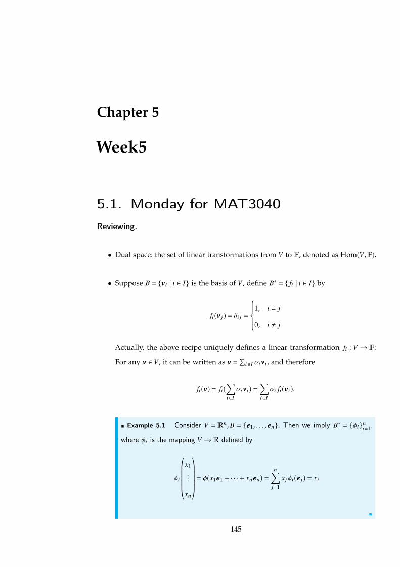
• Dual space: the set of linear transformations from V to F, denoted as Hom(V ,F).
• Suppose B = {vvvi | i 2 I} is the basis of V , define B⇤ = { fi | i 2 I} by
fi(vvv j) = �i j =8>>><>>>:
1, i = j
0, i , j
Actually, the above recipe uniquely defines a linear transformation fi : V ! F:
For any vvv 2 V , it can be written as vvv =Õ
i2I ↵ivvvi, and therefore
fi(vvv) = fi(’i2I
↵ivvvi) =’i2I
↵i fi(vvvi).
⌅ Example 5.1 Consider V = Rn, B = {eee1, . . . ,eeen}. Then we imply B⇤ = {�i}ni=1,
where �i is the mapping V ! R defined by
�i
©≠≠≠≠≠´
x1...
xn
™ÆÆÆÆƨ= �(x1eee1 + · · · + xneeen) =
n’j=1
xj�i(eee j) = xi
⌅
145

5.1.1. Remarks on Dual Space
Proposition 5.1 1. B⇤ is always lienarly independent, i.e., any finite subset of B⇤ is
linearly independent.
2. If V has finite dimension, then B⇤ is a basis of V⇤.
Proof. 1. Suppose that
↵1 fi1 + ↵2 fi2 + · · · + ↵k fik = 000V ⇤ .
In particular, let the input of these linear transformations be vvvi1 , we imply
↵1 fi1(vvvi1) + ↵2 fi2(vvvi1) + · · · + ↵k fik (vvvi1) = 000(vvvi1) ⌘ 000
= ↵1 · 1 + · · · + 0
= ↵1
Applying the same trick, one can show that ↵2 = · · ·=↵k = 0. Therefore, { fi1 , . . . , fik }
is linearly independent.
2. Suppose that B = {vvv1, . . . ,vvvn} and B⇤ = { f1, . . . , fn}. For any f 2 V⇤, construct the
linear transformation
g :=n’i=1
f (vvvi) · fi 2 span{B⇤}.
It follows that for j = 1,2, . . . ,n,
g(vvv j) =n’i=1
f (vvvi) · fi(vvv j) = f (vvv j).
It’s clear that g(vvv) = f (vvv) for all vvv 2 V , i.e., f ⌘ g 2 span(B⇤). Therefore B⇤ spans
V⇤, i.e., forms a basis of V⇤.
⌅
Corollary 5.1 If dim(V) = n, then dim(V⇤) = n.
146

Proof. It’s eay to show the mapping defined as
V ! V⇤
with vvvi 7! fi
is an isomorphism from V ! V⇤. Note that this constructed isomorphism depends on
the choice of basis B in V . (We say this is not a natural isomorphism.) ⌅
R The part 2 for proposition (5.1) does not hold for V with infinite dimension.
The reason is that the spanning set is defined with finite linear combinations.
Check the example below for a counter-example.
⌅ Example 5.2 Suppose that V = F[x], and B⇤ = {1, x, x2, . . . , } forms a basis of V . We
imply that B⇤ = {�0,�1,�2, . . . , }, where �i is the mapping defined as
�i(x j) =8>>><>>>:
1, i = j
0, otherwise
Consider a special element � 2 V⇤ with f (p(x)) = p(1):
�(1) = 1, �(x) = 1, �(x2) = 1, · · · �(xn) = 1, 8n 2 N.
If following the proof in proposition (5.1), we expect that
g :=1’n=0
�(xn)�n =1’n=0
�n 2 span{B⇤},
which is a contradiction, since span{B⇤} consists of finite sum of �i’s only. ⌅
R Therefore, if V is not finite-dimensional, we can say the cardinality of V is
strictly less than the cardinality of V⇤.
Any subspace of a given vector space has some gap. Now we want to describe this
gap formally from the perspective of the dual space.
147

5.1.2. Annihilators
Definition 5.1 Let V be a vector space, S ✓ V be a subset. The annihilator of S is
defined as
Ann(S) = { f 2 V⇤ | f (s) = 0,8s 2 S}
⌅
⌅ Example 5.3 Consider V =R4, B = {eee1, . . . , eee4}. Let B⇤ = { f1, . . . , f4}, S = {eee3, eee4}.
• Then f1 2 Ann(S), since
f1(eee3) = 0, f1(eee4) = 0
Indeed, any a · f1 + b · f2 2 V⇤ is in Ann(S). ⌅
Proposition 5.2 1. The set Ann(S) is a vector subspace of V⇤
2. The mapping Ann(·) is inclusion-reversing, i.e., if W1 ✓ W2 ✓ V , then
Ann(W1) ◆ Ann(W2)
3. The mapping Ann(·) is idempotent, i.e., Ann(S) =Ann(span(S)).
4. If V has finite dimension, and W V , then Ann(W) fills in the gap, i.e.,
dim(W) + dim(Ann(W)) = dim(V)
Proof. 1. Suppose that f ,g 2 Ann(S), i.e., f (s) = g(s) = 0,8s 2 S. It’s clear that (a f +
bg) 2 Ann(S).
2. Suppose that f 2 Ann(W2), we imply f (www) = 0 for any www 2W2. Therefore, f (www1) = 0
for any www1 2 W1 ✓ W2, i.e., f 2 Ann(W1).
3. Note that S ✓ span(S). Therefore we imply Ann(S) ◆ Ann(span(S)) from part (b).
It suffices to show Ann(S) ✓ Ann(span(S)):
148

For any f 2 Ann(S) and anyÕn
i=1 kisssi 2 span(S), we imply
f
n’i=1
kisssi
!=
n’i=1
ki f (sssi)
=
n’i=1
ki · 0
= 0,
i.e., f 2 Ann(span(S)).
4. Let {vvv1, . . . ,vvvk} be a basis of W . By basis extension, we construct a basis of V :
B = {vvv1, . . . ,vvvk ,vvvk+1, . . . ,vvvn}.
Let B⇤ = { f1, . . . , fk , fk+1, . . . , fn} be a basis of V⇤. We claim that { fk+1, . . . , fn} is a
basis of Ann(W):
• Firstly, fj ’s are the elements in Ann(W) for j = k + 1, . . . ,n, since for any
www =Õk
i=1↵i(vvvi) 2 W , we have
fj(www) =k’i=1
↵i fj(vvvi)
=
k’i=1
↵i · 0
= 0, j = k + 1, k + 2, . . . ,n
• Secondly, the set { fk+1, . . . , fn} is linearly independent, since the set B⇤ =
{ f1, . . . , fn} is linearly independent.
• Thirdly, { fk+1, . . . , fn} spans Ann(W): for any g 2 Ann(W) ✓ V⇤, it can be
149
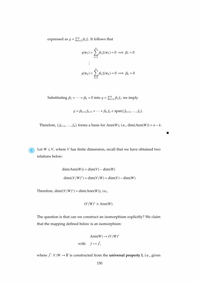
expressed as g =Õn
i=1 �i fi. It follows that
g(vvv1) =n’i=1
�i fi(vvv1) = 0 =) �1 = 0
...
g(vvvk) =n’i=1
�i fi(vvvk) = 0 =) �k = 0
Substituting �1 = · · · = �k = 0 into g =Õn
i=1 �i fi, we imply
g = �k+1 fk+1 + · · · + �n fn 2 span{ fk+1, . . . , fn}.
Therefore, { fk+1, . . . , fn} forms a basis for Ann(W), i.e., dim(Ann(W)) = n � k.
⌅
R Let W V , where V has finite dimension, recall that we have obtained two
relations below:
dim(Ann(W)) = dim(V) � dim(W)
dim((V/W)⇤) = dim(V/W) = dim(V) � dim(W)
Therefore, dim((V/W)⇤) = dim(Ann(W)), i.e.,
(V/W)⇤ � Ann(W).
The question is that can we construct an isomorphism explicitly? We claim
that the mapping defined below is an isomorphism:
Ann(W)! (V/W)⇤
with f 7! f ,
where f : V/W ! F is constructed from the universal property I, i.e., given
150

the mapping f 2 Ann(W), since W ker( f ), there exists f : V/W ! F such
that the diagram below commutes:
i.e., f (vvv +W) = f (vvv).
151

5.4. Wednesday for MAT3040There will be a quiz on next Monday.
Scope : From Week 1 up to (including) the definition of B⇤.
Reviewing.
1. If V is finite dimensional, and B a basis of V , then B⇤ is a basis of the dual space
V⇤.
2. Define the Annihilator Ann(S) V⇤:
Ann(S) = { f 2 V⇤ | f (s) = 0,8s 2 S}
3. If V is finite dimensional, and W V , then Ann(W) fills the gap, i.e.,
dim(Ann(W)) = dim(V) � dim(W)
4. Define a map
� : Ann(W)! (V/W)⇤
f 7! f
where f is defined such that the diagram (5.1) below commutes
Figure 5.1: Construction of f
Or equivalently, f : V/W ! F is such that f (vvv +W) = f (vvv).
160

5.4.1. Adjoint MapThe natural question is that whether � is the isomorphism between Ann(W) and
(V/W)⇤:
Proposition 5.4 � is a linear transformation, i.e.,
�(a f + bg) = a ·�( f ) + b ·�(g).
Proof. Itt suffices to show that
a f + bg = a f + bg
⌅
Therefore, we need to answer whether � a bijective map. We will show this
conjucture at the end of this lecture. The definition of � is natural, i.e., we do not need
to specify any basis to define this � . However, as studied in Monday, the constructed
isomorphism V ! V⇤ with vvvi 7! fi is not natural.
Definition 5.3 [Adjoint Map] Let T : V ! W be a linear transformation. Define the
adjoint of T by
T⇤ : W⇤ ! V⇤
such that for any f 2 W⇤,
[T⇤( f )](vvv) := f (T(vvv)), 8vvv 2 V .
⌅
R
1. In other words, T⇤( f ) = f �T , i.e., a linear transformation from V to F,
i.e., belongs to V⇤.
2. Moreover, the mapping T⇤ itself is a linear transformation: For f ,g 2 W⇤,
161

and 8vvv 2 V ,
[T⇤(a f + bg)](vvv) = (a f + bg)[T(vvv)]
= a f (T(vvv)) + bg(T(vvv)) definition of W⇤ as a vector space
= a[T⇤( f )](vvv) + b[T⇤(g)](vvv)
= [aT⇤( f ) + bT⇤(g)](vvv) definition of V⇤ as a vector space
Proposition 5.5 Let T : V ! W be a linear transformation.
1. If T is injective, then T⇤ is surjective.
2. If T is surjetive, then T⇤ is injective.
This statement is quite intuitive, since T⇤ reverses the dual of output into the dual
of input:
T : V ! W
T⇤ : W⇤ ! V⇤
Proof. We only give a proof of (2), i.e., suffices to show ker(T) = {000}.
Consider any g 2 W⇤ such that T⇤(g) = 000V ⇤ . It follows that
[T⇤(g)](vvv) = 000V ⇤(vvv), 8vvv 2 V . () g(T(vvv)) = 000, 8vvv 2 V . (5.4)
To show g = 000W ⇤ , it suffices to show g(www)= 000 for 8www 2W . For all www 2W , by the surjectivity
of T , there exists vvv0 2 V such that
www = T(vvv0).
By substituting www with T(vvv0) and (5.4), we imply
g(www) = g(T(vvv0)) = 000.
The proof is complete. ⌅
Proposition 5.6 Let T : V ! W be a linear transformation, and A = {vvv1, . . . ,vvvn},B =
{www1, . . . ,wwwm} be the bases of V and W , respectively. Let A⇤ = { f1, . . . , fn},B⇤ = {g1, . . . ,gm}
162

be bases of dual spaces V⇤ and W⇤, respectively. Then T⇤ : W⇤ ! V⇤ admits a matrix
representation
(T⇤)A⇤B⇤ = transpose ((T)BA)
where (T⇤)A⇤B⇤ 2 Fn⇥m and (T)BA 2 F
m⇥n
Proof. Let (T)BA = (↵i j) and (T⇤)A⇤B⇤ = (�i j). By definition of matrix representation,
T(vvv j) =m’i=1
↵i jwwwi, T⇤(gi) =n’
k=1
�ki fk 2 V⇤
As a result,
[T⇤(gi)](vvv j) = gi(T(vvv j))
= gi
m’`=1
↵` jwww`
!
=
m’`=1
↵` jgi(www`)
= ↵i j
and
[T⇤(gi)](vvv j) =
n’k=1
�ki fk
!(vvv j)
=
n’k=1
�ki fk(vvv j)
= �ji
Therefore, �ji = ↵i j . The proof is complete. ⌅
5.4.2. Relationship between Annihilator and dual
of quotient spaces
163

⌅ Example 5.5 Consider the canonical projection mapping ⇡W : V !V/W with its adjoint
mapping:
(⇡W )⇤ : (V/W)⇤ ! V⇤
The understanding of (⇡W )⇤ is as follows:
1. Take h 2 (V/W)⇤ and study (⇡W )⇤(h) 2 V⇤
2. Take vvv 2 V and understand
[(⇡W )⇤(h)](vvv) = h(⇡W (vvv)) = h(vvv +W)
(a) In particular, for all www 2 W V , we have
[(⇡W )⇤(h)](www) = h(www +W) = h(000V/W ) = 000F
Therefore,
(⇡W )⇤(h) 2 Ann(W).
i.e., (⇡W )⇤ is a mapping from (V/W)⇤ to Ann(W).
(b) By proposition (5.5), ⇡W is surjective implies (⇡W )⇤ is injective.
Combining (a) and (b), it’s clear that (i.e., left as homework problem)
� � ⇡⇤W = id(V/W )⇤ and ⇡⇤W �� = idAnn(W )
This relationship implies � is an isomorphism. ⌅
164

Chapter 6
Week6
6.1. Monday for MAT3040
6.1.1. PolynomialsWe recall some useful properties of polynomial before studying eigenvalues/eigenvec-
tors.
Definition 6.1 [Polynomial]
1. A polynomial over F has the form
p(z) = amzm + · · · + a1z + a0, (am , 0).
Here amzm is called the leading term of p(z); m is called the degree; am is called
the leading coefficient; am, · · · ,a0 are called the coefficients of this polynomial.
2. A polynomial over F is monic if its leading coefficient is 1F.
3. A polynomial p(z) 2 F[z] is irreducible if for any a(z), b(z) 2 F[z],
p(z) = a(z)b(z) =) either a(z) or b(z) is a constant polynomial.
Otherwise p(z) is reducible.
⌅
175
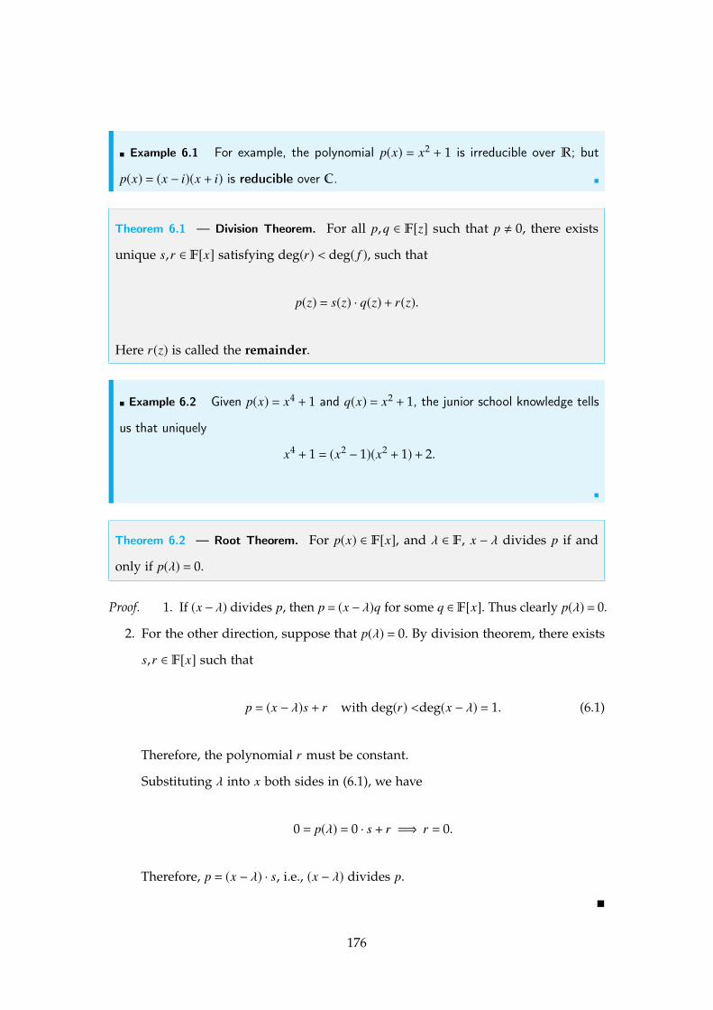
⌅ Example 6.1 For example, the polynomial p(x) = x2 + 1 is irreducible over R; but
p(x) = (x � i)(x + i) is reducible over C. ⌅
Theorem 6.1 — Division Theorem. For all p,q 2 F[z] such that p , 0, there exists
unique s,r 2 F[x] satisfying deg(r) < deg( f ), such that
p(z) = s(z) · q(z) + r(z).
Here r(z) is called the remainder.
⌅ Example 6.2 Given p(x) = x4 + 1 and q(x) = x2 + 1, the junior school knowledge tells
us that uniquely
x4 + 1 = (x2 � 1)(x2 + 1) + 2.
⌅
Theorem 6.2 — Root Theorem. For p(x) 2 F[x], and � 2 F, x � � divides p if and
only if p(�) = 0.
Proof. 1. If (x � �) divides p, then p = (x � �)q for some q 2 F[x]. Thus clearly p(�) = 0.
2. For the other direction, suppose that p(�) = 0. By division theorem, there exists
s,r 2 F[x] such that
p = (x � �)s + r with deg(r) <deg(x � �) = 1. (6.1)
Therefore, the polynomial r must be constant.
Substituting � into x both sides in (6.1), we have
0 = p(�) = 0 · s + r =) r = 0.
Therefore, p = (x � �) · s, i.e., (x � �) divides p.
⌅
176

6.4. Wednesday for MAT3040Reviewing: Root Theorem: p(�) = 0 iff (x � �) divdes p(x).
Corollary 6.2 A polynomial with degree n has at most n roots counting multiplicity.
For example, the polynomial (x � 3)2 has one root x = 3 with multiplicity 2. When
counting multiplicity, we say the polynomial (x � 3)2 has two roots.
Definition 6.5 [Algebraically Closed] A field F is called algebraically closed if every
non-constant polynomial p(x) 2 F[x] has a root � 2 F. ⌅
Theorem 6.5 — Fundamental Theroem of Algebra. The set of complex numbers C is
algebraically closed.
Proof. One way is by complex analysis; Another way is by the topology on C \ {0}. ⌅
R By induction, we can show that every polynomial with degree n on alge-
braically closed field F has exactly n roots, counting multiplicity. Therefore,
for any p(x) on algebraically closed field F,
p(x) = c(x � �1) · · · (x � �n) (6.3)
for c,�1, . . . ,�n 2 F.
The polynomials on general field F may not necessarily be factorized as in (6.3) , but
still admit unique factorization property:
Theorem 6.6 — Unique Factorization. Every f (x) = anxn + · · · + a0 in F[x] can be
factorized as
f (x) = an[p1(x)]e1 · · · [pk(x)]ek
where pi’s are monic, irreducible,distinct. Furthermore, this expression is unique
up to the permutation of factors.
185
Definition 6.6 [Factor] If p(x) = q(x)s(x) with p, q, s 2 F[x], then we say
• p(x) is divisible by s(x);
• s(x) is a factor of p(x);
• s(x)|p(x)
• s(x) divides p(x)
• p(x) is multiple of s(x)
⌅
Definition 6.7 [Common Factor]
1. The polynomial g(x) is said to be a common factor of f1, . . . , fk 2 F[x] if
g | fi, i = 1, . . . , k
2. The polynomial g(x) is said to be a greatest common divisor of f1, . . . , fk if
• g is monic.
• g is common factor of f1, . . . , fk
• g is of largest possible (maximal) degree.
⌅
R
• gcd( f1, . . . , fk) = gcd(gcd( f1, f2), f3, . . . , fk) = gcd(gcd( f1, f2, f3), . . . , fk)
• gcd( f1, . . . , fk) is unique.
• If gcd( f1, . . . , fk) = 1, we say f1, . . . , fk is relatively prime
• Polynomials f1, . . . , fk are relatively prime does not necessarily mean
gcd( fi, fj) = 1 for any i , j.
186

Counter-example: Let a1, . . . ,an distinct irreducible polynomials, and
fi(x) = a1(x) · · · ai(x) · · ·an(x) := a1 · · ·ai�1ai+1 · · ·an,
then gcd( f1, . . . , fn) = 1, but gcd( fi , fj) = a1 · · · ai · · · aj · · ·an, which does not
necessarily equal to 1.
⌅ Example 6.6 The gcd( f1, f2) is easy to compute for factorized polynomials. For example,
let f1(x) = (x2 + x + 1)3(x � 3)2x4 and f2(x) = (x2 + 1)(x � 3)4x2 in R[x], then
gcd( f1, f2) = (x � 3)2x2
⌅
The question is how to find gcd( f1, f2) for given un-factorized polynomials?
Theorem 6.7 — Bezout. Let g = gcd( f1, f2), then there exists r1,r2 2 F[x] such that
g(x) = r1(x) f1(x) + r2(x) f2(x)
More generally, g = gcd( f1, . . . , fk) implies there exists r1, . . . ,rk such that
g = r1 f1 + · · · + rk fk
The derivation of ri’s is by applying Euclidean algorithm. For example, given x3 +
6x + 7 and x2 + 3x + 2, we imply
x3 + 6x + 7 � (x � 3)(x2 + 3x + 2) = 13x + 13
and
x2 + 3x + 2 � x + 213
(13x + 13) = 0
Therefore, gcd(x3 + 6x + 7, x2 + 3x + 2) = gcd(x2 + 3x + 2,13x + 13) = x + 2.
187

6.4.1. Eigenvalues & Eigenvectors
Definition 6.8 [Eigenvalues] Let T : V ! V be a linear operator.
1. We say vvv 2 V \ {000} is an eigenvector of T with eigenvalue � if T(vvv) = �vvv;
2. Or equivalently, vvv 2 ker(T � �I), the �-eigenspace of T . Here the mapping I : V !V
denotes identity map, i.e., I(vvv) = vvv,8vvv 2 V .
⌅
Definition 6.9 A vector vvv 2 V \ {000} is a generalized eigenvector of T with generalized
eigenvalue � if vvv 2 ker((T � �I)k) for some k 2 N+. ⌅
Note that an eigenvector is a generalized eigenvector of T ; while the converse does not
necessarily hold.
⌅ Example 6.7 Consider the linear transformation A : R2 ! R
2 with
A : R2 ! R
2
with xxx ! AAAxxx
where AAA =©≠≠´1 1
0 1
™Æƨ
1. Note that [1,0]T is an eigenvector with eigenvalue 1, since
A©≠≠´1
0
™Æƨ=
©≠≠´1
0
™Æƨ
2. However, [0,1]T is not an eigenvector, since
A©≠≠´0
1
™Æƨ=
©≠≠´1
0
™Æƨ
.
188
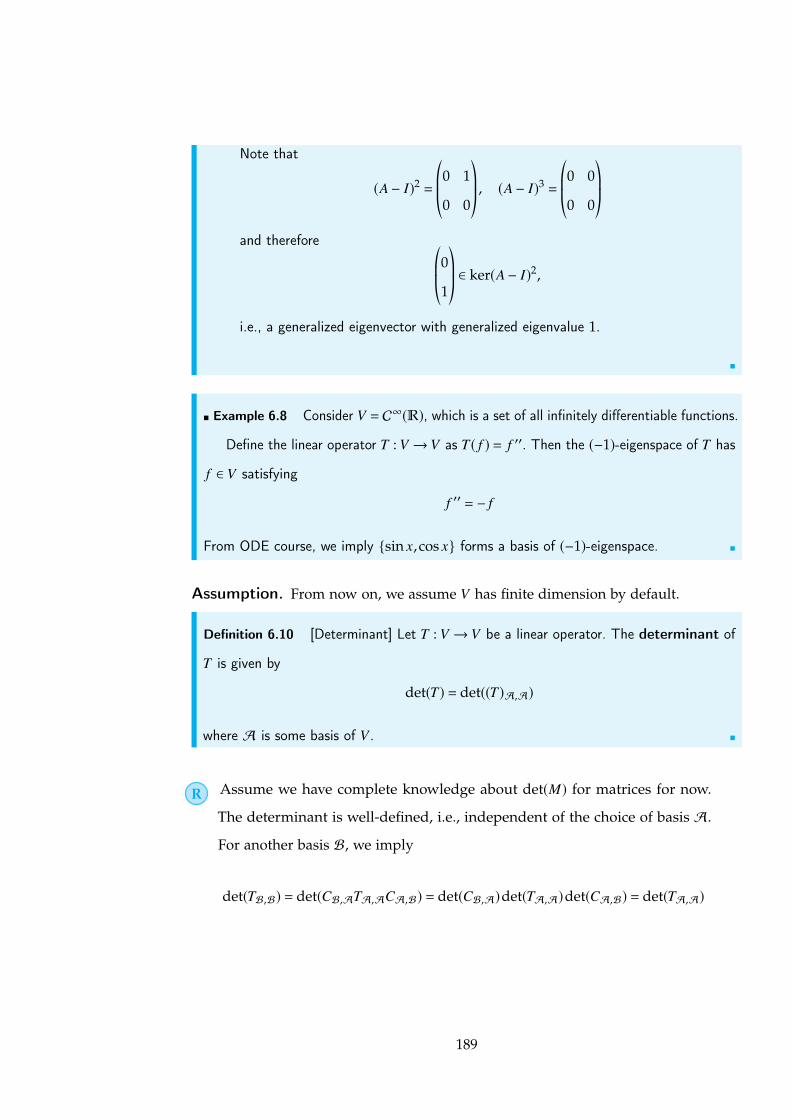
Note that
(A� I)2 =©≠≠´0 1
0 0
™Æƨ
, (A� I)3 =©≠≠´0 0
0 0
™Æƨ
and therefore©≠≠´0
1
™Æƨ2 ker(A� I)2,
i.e., a generalized eigenvector with generalized eigenvalue 1.
⌅
⌅ Example 6.8 Consider V = C1(R), which is a set of all infinitely differentiable functions.
Define the linear operator T : V !V as T( f ) = f 00. Then the (�1)-eigenspace of T has
f 2 V satisfying
f 00 = � f
From ODE course, we imply {sin x, cos x} forms a basis of (�1)-eigenspace. ⌅
Assumption. From now on, we assume V has finite dimension by default.
Definition 6.10 [Determinant] Let T : V ! V be a linear operator. The determinant of
T is given by
det(T) = det((T)A,A)
where A is some basis of V . ⌅
R Assume we have complete knowledge about det(M) for matrices for now.
The determinant is well-defined, i.e., independent of the choice of basis A.
For another basis B, we imply
det(TB,B) = det(CB,ATA,ACA,B) = det(CB,A)det(TA,A)det(CA,B) = det(TA,A)
189
Definition 6.11 [characteristic polynomial] The characteristic polynomial XT (x) of
T : V ! V is defined as
XT (x) = det((T)A,A � xI)
for any basis A ⌅
In the next few lectures, we will study
• Cayley-Hamilton Theorem
• Jordan Canonical Form
These theorems can be stated using matrices, and they both hold up to change of
basis. We have a unified statement of these theorem using vecotor space rather than
Rn.
190

Chapter 7
Week7
7.1. Monday for MAT3040Reviewing. Define the characteristic polynomial for an linear operator T :
XT (x) = det((T)A,A � xIII)
We will use the notation “I/III” in two different occasions:
1. I denotes the identity transformation from V to V with I(vvv) = vvv,8vvv 2 V
2. III denotes the identity matrix (I)A,A , defined based on any basis A.
7.1.1. Minimal Polynomial
Definition 7.1 [Linear Operator Induced From Polynomial] Let f (x) := amxm + · · · + a0
be a polynomial in F[x], and T : V ! V be a linear operator. Then the mapping
f (T) = amTm + · · · + a1T + a0I : V ! V ,
is called a linear operator induced from the polynomial f (x). ⌅
R
1. The composition of linear operators is not abelian, e.g., in general S �T =
T � S does not hold. The reason follows similarly from the fact that
square-matrix multiplication is not abelian in general.
193

2. However, we always have f (T)T = T f (T), where f (T) is a linear operator
induced from the polynomial f (x):
Proof. We can show that TnT =TTn,8n by induction. Suppose that f (x) =Õi aixi, which follows that
f (T)T =’i
aiT iT =’i
aiTT i = T’i
aiT i = T f (T).
⌅
3. We can generalize the statement in (2) into the fact that the composition
of linear operators induced from polynomials is abelian, i.e.,
f (T)g(T) = g(T) f (T)
for any polynomials f (x),g(x).
Definition 7.2 [Minimal Polynomial] Let T : V ! V be a linear operator. The minimal
polynomial mT (x) is a nonzero monic polynomial of least (minimal) degree such that
mT (T) = 000V!V .
where 000V!V denotes the zero vector in Hom(V ,V). ⌅
⌅ Example 7.1 1. Let AAA =©≠≠´1 0
0 1
™Æƨ, then AAA defines a linear operator:
A : F2 ! F
2
with xxx 7! AAAxxx
Here XA(x) = (x � 1)2 and AAA� III = 000, which gives mA(x) = x � 1.
194

2. Let BBB =©≠≠´1 1
0 1
™Æƨ, which implies
XB(x) = (x � 1)2,
The question is that can we get the minimal polynomial with degree 1?
The answer is no, since BBB � kIII =©≠≠´1 � k 1
0 1 � k
™Æƨ, 000.
In fact, mB(x) = (x � 1)2, since
(BBB � III)2 =©≠≠´0 1
0 0
™Æƨ
2
=©≠≠´0 0
0 0
™Æƨ
.
⌅
Two questions naturally arises:
1. Does mT (x) exist? If exists, is it unique?
2. What’s the relationship between mT (x) and XT (x)?
Regarding to the first question, the minimal polynomial mT (x) may not exist, if V has
infinite dimension:
⌅ Example 7.2 Consider V =R[x] and the mapping
T : V ! V
p(x) 7!Ø x
0 p(t)dt
In particular, T(xn) = 1n+1 xn+1. Suppose mT (x) is with degree n, i.e.,
mT (x) = xn + · · · + a1x + a0,
then
mT (T) = Tn + · · · + a0I is a zero linear transformation
195

It follows that
[mT (T)](x) =1n!
xn + an�11
(n � 1)! xn�1 + · · · + a1x + a0 = 0F,
which is a contradiction since the coefficients of xk is nonzero on LHS for k = 1, . . . ,n, but
zero on the RHS. ⌅
Proposition 7.1 The minimal polynomial mT (x) always exists for dim(V) = n <1.
Proof. It’s clear that {I,T , . . . ,Tn,Tn+1, · · · ,Tn2} ✓ Hom(V ,V). Since dim(Hom(V ,V)) = n2,
we imply {I,T , . . . ,Tn,Tn+1, · · · ,Tn2} is linearly dependent, i.e., there exists ai’s that are
not all zero such that
a0I + a1T + · · · + an2Tn2= 0
i.e., there is a polynomial g(x) of degree less than n2 such that g(T) = 0.
The proof is complete. ⌅
Proposition 7.2 The minimal polynomial mT (x), if exists, then it exists uniquely.
Proof. Suppose f1, f2 are two distinct minimal polynomials with deg( f1) = deg( f2). It
follows that
• deg( f1 � f2) < deg( f1).
• f1 � f2 , 0
• ( f1 � f2)(T) = f1(T) � f2(T) = 0V!V
By scaling f1 � f2, there is a monic polynomial g with lower degree satisfying g(T) = 0,
which contradicts the definition for minimal polynomial. ⌅
Proposition 7.3 Suppose f (x) 2 F[x] satisfying f (T) = 000, then
mT (x) | f (x).
Proof. It’s clear that deg( f ) � deg(mT ). The division algorithm gives
f (x) = q(x)mT (x) + r(x).
196
Therefore, for any vvv 2 V
[r(T)](vvv) = [ f (T)](vvv) � [q(T)mT (T)](vvv) = 000V � q(T)000V = 000V � 000V = 000V
Therefore, r(T) = 000V!V . By definition of minimal polynomial, we imply r(x) ⌘ 0. ⌅
Proposition 7.4 If AAA, BBB 2 Fn⇥n are similar to each other, then mA(x) = mB(x).
Proof. Suppose that BBB = PPP�1 AAAPPP, and that
mA(x) = xk + · · · + a1x + a0, mB(x) = x` + · · · + b0.
It follows that
mA(BBB) = BBBk + · · · + a0I
= PPP�1 AAAkPPP + · · · + a0PPP�1PPP
= PPP�1(AAAk + · · · + a0III)PPP
= PPP�1(mA(AAA))PPP
Therefore, mA(BBB) = 000 since mA(AAA) = 000. By proposition (7.3), we imply mB(x) | mA(x).
Similarly, mA(x) | mB(x). Since mA(x) and mB(x) are monic, we imply mA(x) = mB(x). ⌅
R Proposition (7.4) claims that the minimal polynomial is similarity-invariant;
actually, the characteristic polynomial is similarity-invariant as well.
Assumption. We will asssume V has finite dimension from now on. Now we study
the vanishing of a single vector vvv 2 V .
Notation. The mT (x) is a nonzero monic poylnomial of least degree such that
mT (T) = 000V!V .
197
7.1.2. Minimal Polynomial of a vector
Definition 7.3 [Minimal Polynomial of a vector] Similar to the minimal polynomial, we
define the minimal polynomial of a vector vvv relative to T , say mT ,vvv(x), as the monic
polynomial of least degree such that
mT ,vvv(T)(vvv) = 0
⌅
The existence of minimal polynomial of a vector is due to the existence of minimal
polynomial; the uniqueness follows similarly as in proposition (7.2).
Proposition 7.5 Let T : V !V be a linear operator and vvv 2V . The degree of the minimal
polynomial of a vector is upper bounded by:
deg(mT ,vvv(x)) dim(V).
Proof. It’s clear that {vvv,Tvvv, . . . ,Tnvvv} ✓ V and the proof follows similarly as in proposi-
tion (7.1). ⌅
Similar to the division property in proposition (7.3), we have the division proprty
for minimal polynomial of a vector:
Proposition 7.6 Suppose f (x) 2 F[x] satisfying f (T)(vvv) = 000V , then
mT ,vvv(x) | f (x).
In particular, mT ,vvv | mT (x).
Proof. The proof follows similarly as in proposition (7.3). ⌅
Proposition 7.7 Suppose that mT ,vvv(x) = f1(x) f2(x), where f1, f2 are both monic. Let
www = f1(T)vvv, then
mT ,www(x) = f2(x)
198

Proof. 1.
f2(T)www = f2(T) f1(T)vvv = mT ,vvv(T)vvv = 000
By the proposition (7.3), we imply mT ,www | f2.
2. On the other hand,
000 = mT ,www(T)(www) = mT ,www(T) f1(T)vvv = f1(T)mT ,www(T)vvv,
which implies that mT ,vvv(x) | f1(x)mT ,www(x),, i.e.,
f1 · f2 | f1 · mT ,www =) f2 | mT ,www .
The proof is complete.
⌅
199
7.4. Wednesday for MAT3040Reviewing.
• Given the polynomial f (x) 2 F[x], we extend it into the linear operator f (T) : V !
V .
• The minimal polynomial mT (x) is defined to be the polynomial with least degree
such that
mT (T) = 000V!V ,
i.e., [mT (T)]vvv = 0VVV ,8vvv 2 V .
• The minimial polynomial of a vector vvv relative to T is defined to be the polynomial
mT ,vvv(x) with the least degree such that
mT ,vvv(T)(vvv) = 0
• If f (T) = 000V!V , then we imply mT (x) | f (x). If [g(T)](www) = 0V , following the similar
argument, we imply mT ,www(x) | g(x).
• In particular, mT (T)www = 000, which implies mT ,www(x) | mT (x).
7.4.1. Cayley-Hamiton TheoremLet’s raise an motivative example first:
⌅ Example 7.8 Consider the matrix and its induced mapping AAA =©≠≠´1 0
0 2
™Æƨ. It has the
characteristic polynomial
XA = (x � 1)(x � 2).
• Note that mA(x) cannot be with degree one, since otherwise mA(x) = x � k with
211

some k, and
mA(AAA) = AAA� kIII =©≠≠´1 � k 0
0 2 � k
™Æƨ, 000, 8k,
which is a contradiction.
• However, one can verify that the mA(x) is with degree 2:
mA(x) = (x � 1)(x � 2).
• The minimial polynomial with eigenvectors can be with degree 1:
www = [0,1]T =) (A� 2I)www = 000 =) mA,www(x) = x � 2
⌅
R More generally, given an eigen-pair (�,vvv), the minimal polynomial of an vvv
has the explicit form
mT ,vvv(x) = (x � �) =) (x � �) | mT (x)
Now we want to relate the characterstic polynomial mT (x) with XT (x). Sup-
pose that
XT (x) = (x � �1)e1 · · · (x � �k)ek 2 F[x]. (7.1)
Then we imply
• �i is an eigenvalue of T ;
• (x � �i) | mT (x);
which implies that (x � �1) · · · (x � �k) | mT (x).
Furthermore, (a). does mT (x) possess other factors, e.g., does there exist
µ , �i, i = 1, . . . , k such that (x � µ) | mT (x)? (b). does (x � �i) fi | mT (x) when
fi > ei?
The answer is no for both question (a) and (b).
212

Theorem 7.1 — Cayley-Hamilton. mT (x) | XT (x). In particular, XT (T) = 000.
The nice equality in (7.1) does not necessarily hold. Sometimes XT (x) cannot be
factorized into linear factors in F[x], e.g., A =©≠≠´0 �1
1 0
™Æƨ
in R.
However, for every f (x) 2 F[x], we can extend F into the algebraically closed set
F ◆ F such that
f (x) = (x � �1)e1 · · · (x � �k)ek
where �i 2 F.
For example, for f (x) = x2 + 1 2 R[x], we can extend R into C to obtain
f (x) = (x + i)(x � i).
Therefore, the general proof outline for the Cayley-Hamilton Theorem is as follows:
• Consider the case where mT (x),XT (x) are both in F[x]
• Show that mT (x) | XT (x) under F[x].
Before the proof, let’s study the invariant subspaces, which leads to the decomposi-
tion of charactersitc polynomial:
Assumption. From now on, we assume that V is finite dimensional by default.
Definition 7.12 [Invariant Subspace] An invariant subspace of a linear operator T :
V ! V is a subspace W V that is preserved by T, i.e., T(W) ✓ W . We also call W as
T-invariant. ⌅
R If W V is T-invariant, then the restriction of the linear operator T : V ! V
induces the linear operator
T |W : W ! W .
213
⌅ Example 7.9 1. V itself is T-invariant.
2. For the eigenvalue �, the associated �-eigenspace U = ker(T � �I) is T-invariant.
3. More generally, U = ker(g(T)) is T-invariant for any polynomial g:
If vvv 2 ker(g(T)), i.e., g(T)vvv = 000, it suffices to show T(vvv) 2 ker(g(T)):
g(T)[T(vvv)] = (amTm + · · · + a0I)[T(vvv)]
= (amT �Tm + · · · + a1T �T + a0T � I)(vvv)
= T[g(T)vvv] = T(000) = 000
4. For vvv 2 ker(T � �I), U = span{vvv} is T-invariant.
⌅
Proposition 7.10 Suppose that T : V ! V is a linear transformation and W V is
T-invariant, then we construct the subspace mapping and the recipe mapping
T |W : W ! W
with www 7! T(www)(7.2a)
T : V/W ! V/W
with vvv +W 7! T(vvv) +W(7.2b)
(Here the well-definedness of the recipe mapping T is shown in Hw2, Exercise 4),
which leads to the decomposition of the charactersitic polynomial:
XT (x) = XT |W (x)XT (x).
Proof. Suppose C = {vvv1, . . . ,vvvk} is a basis of W , and extend it into the basis of V , denoted
as
B = {vvv1, . . . ,vvvk ,vvvk+1, . . . ,vvvn}
Therefore, B = {vvvk+1 +W , . . . ,vvvn +W} is a basis of V/W . By Homework 2, Question 5,
214

the representation (T)B,B can be written as the block matrix
(T)B,B =©≠≠´(T |W )C,C ⇥
000 (T)B,B
™Æƨ(k+(n�k))⇥(k+(n�k))
Therefore, the characteristic polynomial of T can be calculated as:
XT (x) = det((T)B,B � xI)
= det((T |U )C,C � xI) · det((T)B,B � xI)
⌅
Proposition 7.11 Suppose that
XT (x) = (x � �1) · · · (x � �n)
where �i’s are not necessarily distinct. Then there exists a basis of V , say A, such that
(T)A,A =
©≠≠≠≠≠≠≠≠´
�1 ⇥ ⇥ ⇥
0 �2 · · · ⇥
0 · · · . . . ⇥
0 0 · · · �n
™ÆÆÆÆÆÆÆƨ
Proof. The proof is by induction on n, i.e., suppose the results hold for all vector
spaces with dimension no more than n � 1, and we aim to show this result holds for
dimension n.
1. Step 1: Argue that there exists the associated eigenvector vvv of �1 under the linear
operator T .
Consider any basis M, by MAT2040, there exists associated eigenvector of �1, say
yyy 2 Cn such that
(T)M,M · yyy = �1yyy
Since the operator (·)M : V ! Cn is an isomorphism, there exists vvv 2 V \ {000} such
215
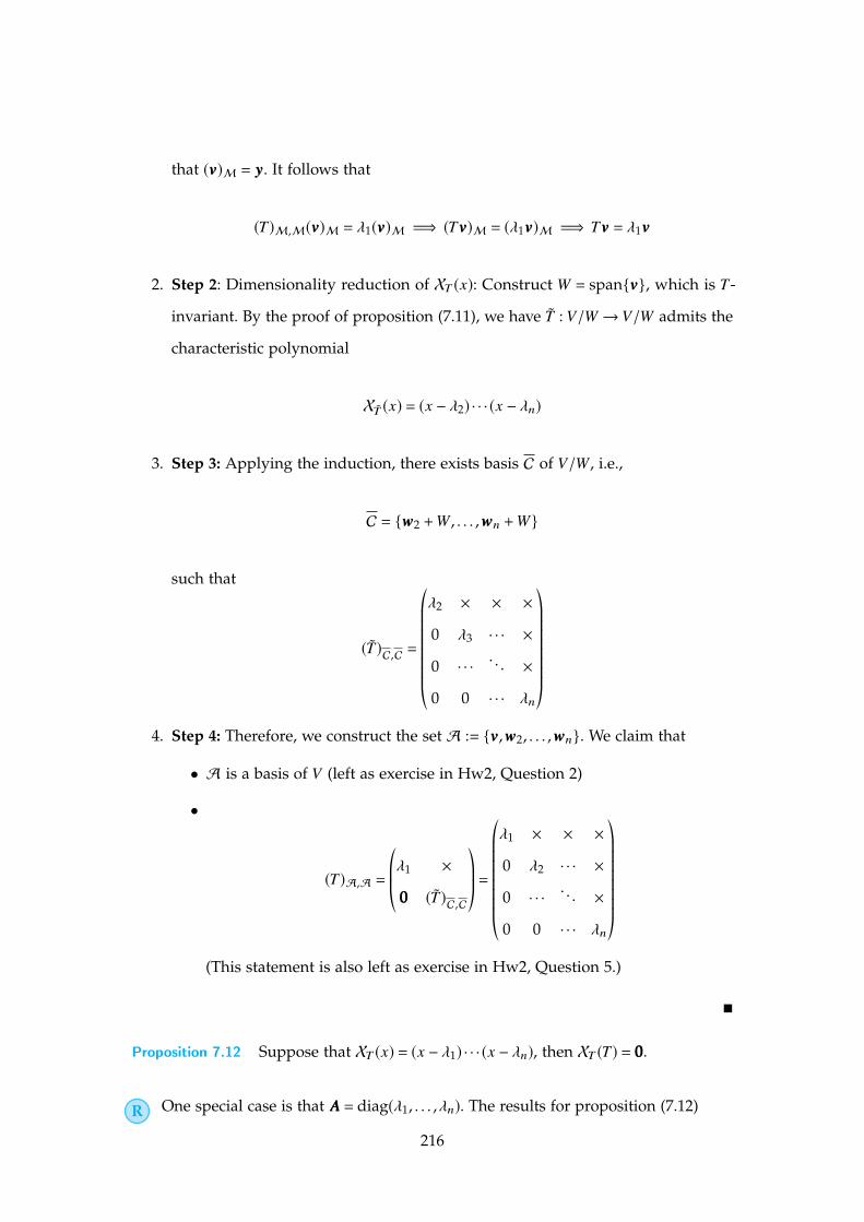
that (vvv)M = yyy. It follows that
(T)M,M(vvv)M = �1(vvv)M =) (Tvvv)M = (�1vvv)M =) Tvvv = �1vvv
2. Step 2: Dimensionality reduction of XT (x): Construct W = span{vvv}, which is T-
invariant. By the proof of proposition (7.11), we have T : V/W ! V/W admits the
characteristic polynomial
XT (x) = (x � �2) · · · (x � �n)
3. Step 3: Applying the induction, there exists basis C of V/W , i.e.,
C = {www2 +W , . . . ,wwwn +W}
such that
(T)C,C =
©≠≠≠≠≠≠≠≠´
�2 ⇥ ⇥ ⇥
0 �3 · · · ⇥
0 · · · . . . ⇥
0 0 · · · �n
™ÆÆÆÆÆÆÆƨ
4. Step 4: Therefore, we construct the set A := {vvv,www2, . . . ,wwwn}. We claim that
• A is a basis of V (left as exercise in Hw2, Question 2)
•
(T)A,A =©≠≠´�1 ⇥
000 (T)C,C
™Æƨ=
©≠≠≠≠≠≠≠≠´
�1 ⇥ ⇥ ⇥
0 �2 · · · ⇥
0 · · · . . . ⇥
0 0 · · · �n
™ÆÆÆÆÆÆÆƨ
(This statement is also left as exercise in Hw2, Question 5.)
⌅
Proposition 7.12 Suppose that XT (x) = (x � �1) · · · (x � �n), then XT (T) = 000.
R One special case is that AAA = diag(�1, . . . ,�n). The results for proposition (7.12)
216

gives
(A� �1III) · · · (A� �nIII) is a zero matrix
217


Chapter 8
Week8
8.1. Monday for MAT3040Reviewing.
• If XT (x) = (x � �1) · · · (x � �n), then
(T)A,A =
©≠≠≠≠≠≠≠≠´
�1 ⇥ ⇥ ⇥
0 �2 · · · ⇥
0 · · · . . . ⇥
0 0 · · · �n
™ÆÆÆÆÆÆÆƨ
for some basis A. In other words, T is triangularizable with the diagonal entries
�1, . . . ,�n.
R I hope you appreciate this result. Consider the example below: In linear
algebra we have studied that the matrix AAA =©≠≠´1 1
0 1
™Æƨ
is not diagonalizable, and
the characteristic polynomial is given by
XA(x) = (x � 1)2.
However, the theorem above claims that AAA is triangularizable, with diagonal
entries 1 and 1. The diagonalization of AAA only uses the eigenvector of AAA, but
the 1-eigenspace has only 1 dimension. Fortunately, the triangularization
gives a rescue such that we can make use of the generalized eigenvector
225

(0,1)T (but not an eigenvector) of AAA by considering the mapping below:
U = span
8>>><>>>:©≠≠´1
0
™Æƨ
9>>>=>>>;
A : V/U ! V/U
Here (0,1)T +U is an eigenvector of A, with eigenvalue 1.
Theorem 8.1 The linear operator T is triangularizable with diagonal entries (�1, . . . ,�n)
if and only if
XT = (x � �1) · · · (x � �n)
Proof. It suffices to show only the sufficiency. Suppose that there exists basis A such
that
(T)A,A =
©≠≠≠≠≠≠≠≠´
�1 ⇥ ⇥ ⇥
0 �2 · · · ⇥
0 · · · . . . ⇥
0 0 · · · �n
™ÆÆÆÆÆÆÆƨ
Then we compute the characteristic polynomial directly:
XT (x) = det[(xI �T)A,A]
= det
©≠≠≠≠≠≠≠≠´
x � �1 ⇥ ⇥ ⇥
0 x � �2 · · · ⇥
0 · · · . . . ⇥
0 0 · · · x � �n
™ÆÆÆÆÆÆÆƨ
= (x � �1) · · · (x � �n)
⌅
226

8.1.1. Cayley-Hamiton TheoremProposition 8.1 — A Useful Lemma. Suppose that XT (x) = (x � �1) · · · (x � �n), then
XT (T) = 0.
Proof. Since XT (x) = (x � �1) · · · (x � �n), we imply T is triangularizable under some basis
A. Note that
• T 7! (T)A,A is an isomorphism between Hom(V ,V) and Mn⇥n(F),
• (T �T � · · · �T| {z }m times
)A,A = [(T)A,A]m, for any m,
It suffices to show XT ((T)A,A) is the zero matrix (why?):
XT ((T)A,A) = ((T)A,A � �1III) · · · ((T)A,A � �nIII).
Observe the matrix multiplication
((T)A,A � �i III)
©≠≠≠≠≠≠≠≠≠≠≠≠≠≠≠´
x1...
xi
0...
0
™ÆÆÆÆÆÆÆÆÆÆÆÆÆÆƨ
=
©≠≠≠≠≠≠≠≠´
�1 � �i ⇥ ⇥ ⇥
0 �2 � �i · · · ⇥
0 · · · . . . ⇥
0 0 · · · �n � �i
™ÆÆÆÆÆÆÆƨ
©≠≠≠≠≠≠≠≠≠≠≠≠≠≠≠´
x1...
xi
0...
0
™ÆÆÆÆÆÆÆÆÆÆÆÆÆÆƨ
2 span{eee1, . . . , eeei�1}
Therefore, for any vvv 2 V ,
((T)A,A � �nIII)vvv 2 span{eee1, . . . , eeen�1}.
Applying the same trick, we conclude that
((T)A,A � �1III) · · · ((T)A,A � �nIII)vvv = 000, 8vvv 2 V ,
i.e., XT ((T)A,A) = ((T)A,A � �1III) · · · ((T)A,A � �nIII) is a zero matrix. ⌅
Now we are ready to give a proof for the Cayley-Hamiton Theorem:
227

Proof. Suppose that XT (x) = xn + an�1xn�1 + · · · + a0 2 F[x]. By considering algebrically
closed field F ◆ F, we imply
XT (x) = xn + an�1xn�1 + · · · + a0 (8.1a)
= (x � �1) · · · (x � �n), �i 2 F (8.1b)
By applying proposition (8.1), we imply XT (T) = 0, where the coefficients in the formula
XT (T) = 0 w.r.t. T are in F.
Then we argue that these coefficients are essentially in F. Expand the whole map
of XT (T):
XT (T) = (T � �1I) · · · (T � �nI) (8.2a)
= Tn � (�1 + · · · + �n)Tn�1 + · · · + (�1)n�1 · · ·�nI (8.2b)
= Tn + an�1Tn�1 + · · · + a0I (8.2c)
where the derivation of (8.2c) is because that the polynomial coefficients for (8.1a) and
(8.1b) are all identical.
Therefore, we conclude that XT (T) = 0, under the field F. ⌅
Corollary 8.1 mT (x) | XT (x). More precisely, if
XT (x) = [p1(x)]e1 · · · [pk(x)]ek , ei > 0,8i
where pi’s are distinct, monic, and irreducible polynomials. Then
mT (x) = [p1(x)] f1 · · · [pk(x)] fk , for some 0 < fi ei,8i
Proof. The statement mT (x) | XT (x) is from Cayley-Hamiton Theorem. Therefore, 0
fi ei,8i. Suppose on the contrary that fi = 0 for some i. w.l.o.g., i = 1.
It’s clear that gcd(p1, pj) = 1 for 8 j , 1, which implies
a(x)p1(x) + b(x)pj(x) = 1, for some a(x), b(x) 2 F[x].
228

Considering the field extension F ◆ F, we have p1(x) = (x � µ1) · · · (x � µ`). For any
root µm of p1, m = 1, . . . ,`, we have
a(µm)p1(µm) + b(µm)pj(µm) = 1 =) b(µm)pj(µm) = 1 =) pj(µm) , 0,
i.e., µm is not a root of pj , 8 j , 1.
Therefore, µm is a root of XT (x), but not a root of mT (x). Then µm is an eigenvalue of
T , e.g., Tvvv = µmvvv for some vvv , 000. Recall that mT ,vvv = x � µm, we imply mT ,vvv = x � µm | mT (x),
which is a contradiction. ⌅
⌅ Example 8.1 We can use Corollary (8.1), a stronger version of Cayley-Hamiltion
Theorem to determine the minimal polynomials:
1. For matrix AAA=©≠≠´0 �1
1 1
™Æƨ, we imply XA(x)= (x2 + x + 1)1. Since x2 + x + 1 is irreducible
in R, we have mA(x) = x2 + x + 1.
2. For matrix
AAA =
©≠≠≠≠≠≠≠≠´
1 1 0 0
0 1 0 0
0 0 2 0
0 0 0 2
™ÆÆÆÆÆÆÆƨ
,
we imply XA(x) = (x � 1)2(x � 2)2.
By Corollary (8.1), we imply both (x � 1) and (x � 2) should be roots of mT (x), i.e.,
mA(x) may have the four options:
(x � 1)2(x � 2)2, or
(x � 1)(x � 2)2, or
(x � 1)2(x � 2), or
(x � 1)(x � 2).
By trial and error, one sees that mA(x) = (x � 1)2(x � 2).
229

⌅
8.1.2. Primary Decomposition Theorem
We know that not every linear operator is diagonalizable, but diagonalization has some
nice properties:
Definition 8.1 [diagonalizable] The linear operator T : V ! V is diagonalizable over F if
and only if there exists a basis A of V such that
(T)A,A = diag(�1, . . . ,�n),
where �i’s are not necessarily distinct. ⌅
Proposition 8.2 If the linear operator T : V ! V is diagonalizable, then
mT (x) = (x � µ1) · · · (x � µk),
where µi’s are distinct.
Proof. Suppose T is diagonalizable, then there exists a basis A of V such that
(T)A,A = diag(µ1, . . . , µ1, µ2, . . . , µ2, . . . , µk , . . . , µk)
It’s clear that ((T)A,A � µ1III) · · · ((T)A,A � µk III) = 000, i.e., mT (x) | (x � µ1) · · · (x � µk).
Then we show the minimality of (x � µ1) · · · (x � µk). In particular, if (x � µi) is
omitted for any 1 i k, then it’s easy to show
(TA,A � µ1III) · · · (TA,A � µi�1III)(TA,A � µi+1III) · · · (TA,A � µk III) , 000,
since all µi’s are distinct. Therefore, mT (x) will not divide (x � µ1) · · · (x � µi�1)(x �
µi+1) · · · (x � µk) for any i, i.e.,
mT (x) = (x � µ1) · · · (x � µk)
230

⌅
R The converse of proposition (8.2) is also true, which is a special case for the
Primary Decomposition Theorem.
Theorem 8.2 — Primary Decomposition Theorem. Let T : V ! V be a linear operator
with
mT (x) = [p1(x)]e1 · · · [pk(x)]ek ,
where pi’s are distinct, monic, and irreducible polynomials. Let Vi = ker([pi(x)]ei )
V , i = 1, . . . , k, then
1. Each Vi is T-invariant (T(Vi) Vi)
2. V = V1 � V2 � · · · � Vk
3. Consider T |Vi : Vi ! Vi, then
mT |Vi (x) = [pi(x)]ei
231
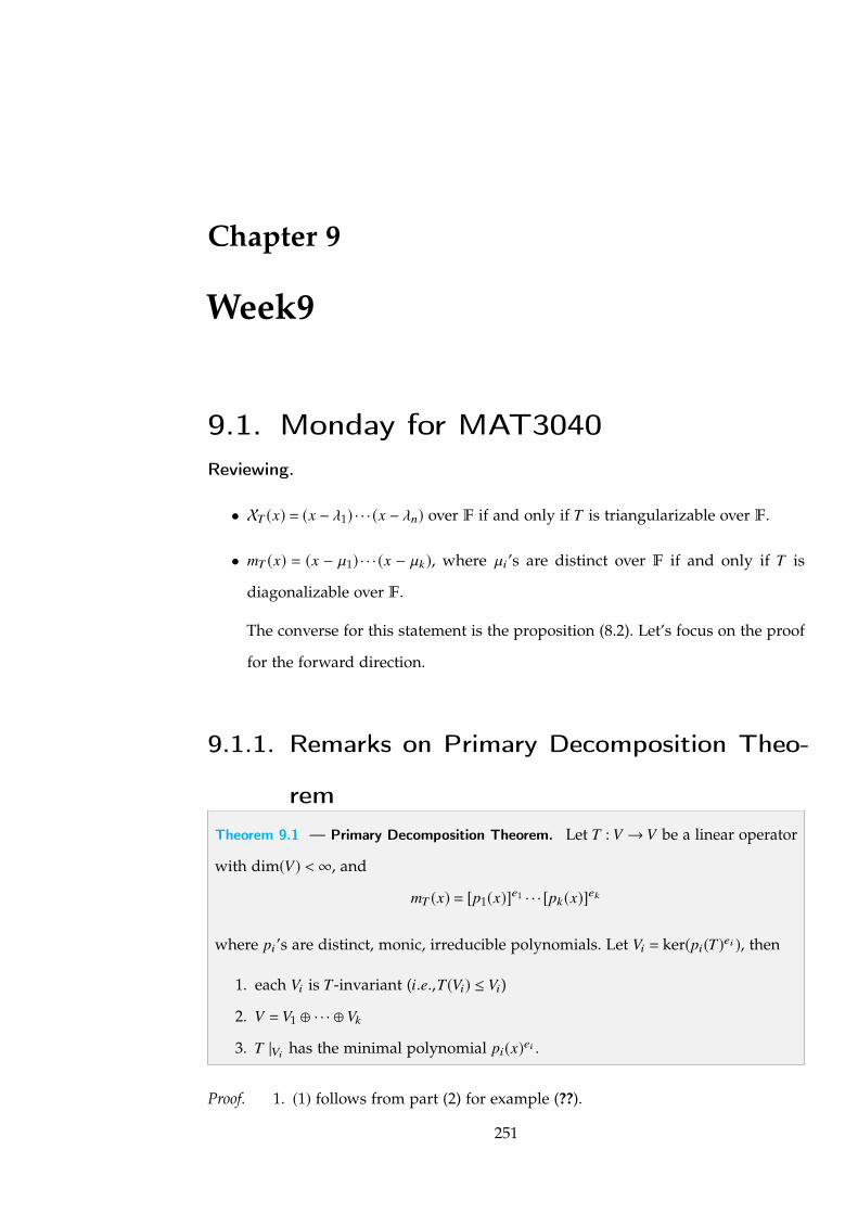
Chapter 9
Week9
9.1. Monday for MAT3040Reviewing.
• XT (x) = (x � �1) · · · (x � �n) over F if and only if T is triangularizable over F.
• mT (x) = (x � µ1) · · · (x � µk), where µi’s are distinct over F if and only if T is
diagonalizable over F.
The converse for this statement is the proposition (8.2). Let’s focus on the proof
for the forward direction.
9.1.1. Remarks on Primary Decomposition Theo-
remTheorem 9.1 — Primary Decomposition Theorem. Let T : V ! V be a linear operator
with dim(V) <1, and
mT (x) = [p1(x)]e1 · · · [pk(x)]ek
where pi’s are distinct, monic, irreducible polynomials. Let Vi = ker(pi(T)ei ), then
1. each Vi is T-invariant (i.e.,T(Vi) Vi)
2. V = V1 � · · · � Vk
3. T |Vi has the minimal polynomial pi(x)ei .
Proof. 1. (1) follows from part (2) for example (??).
251
2. Let qi(x) = [p1(x)]e1 · · · ú[pi(x)]ei · · · [pk(x)]ek := mT (x)/[pi(x)]ei , then it is clear that
(a) gcd(q1, . . . , qk) = 1
(b) gcd(qi, peii ) = 1
(c) qi · peii = mT
(d) If i , j, then mT (x) | qi(x)qj(x)
• By (a) and Bezout’s Theorem (6.7), there exists polynomials a1, . . . ,ak such
that
a1(x)q1(x) + · · · + ak(x)qk(x) = 1,
which implies
a1(T)q1(T)vvv| {z }vvv1
+ · · · + ak(T)qk(T)vvv| {z }vvvk
= vvv
Therefore, vvv = vvv1 + · · · + vvvk for our constructed vvv1, . . . ,vvvk .
• Note that
pi(T)ei vvvi = pi(T)ei ai(T)qi(T)vvv = ai(T)[qi(T)pi(T)ei ]vvv = ai(T)mT (T)vvv = 000,
whcih implies vvvi 2 ker([pi(T)]ei ) := Vi, and therefore
V = V1 + · · · +Vk (9.1)
• To show that the summation in (9.3) is essentially the direct sum, consider
000 = vvv01 + · · · + vvv0k , 8vvv0i 2 Vi. (9.2)
By (a) and Bezout’s Theorem (6.7), there exists bi(x),ci(x) such that
bi(x)qi(x) + ci(x)pi(x)ei = 1 =) bi(T)qi(T) + ci(T)pi(T)ei = I,
i.e.,
bi(T)qi(T)vvv0i + ci(T)pi(T)ei vvv0i = bi(T)qi(T)vvv0i = vvv0i.
252
Appying the mapping bi(T)qi(T) into equality (9.4) both sides, i = 1, . . . , k,
we obtain
000 = bi(T)qi(T)000 = bi(T)qi(T)vvv01 + · · · + bi(T)qi(T)vvv0k
Note that all terms on RHS vanish except for bi(T)qi(T)vvv0i = vvv0i, since qi(x) =
[p1(x)]e1 · · · ú[pi(x)]ei · · · [pk(x)]ek and vvv0j 2 ker([pj(x)]e j ). Therefore, vvv0i = 0 for
i = 1, . . . , k, i.e., V = V1 � · · · � Vk .
3. For any vvvi 2 Vi, we have pi(T)ei vvvi = 000, which implies mT |Vi (x) | pi(x)ei . Together
with Corollary (8.1), mT |vi (x) = pi(x) fi for some 1 fi ei.
Suppose on the contrary that there exists fi < ei for some i, consider any vvv :=
vvv1 + · · · + vvvk 2 V , and
p1(T) f1 · · · pk(T) fk vvv = p1(T) f1 · · · pk(T) fk (vvv1 + · · · + vvvk)
The term on the RHS vanishes since pj(T) fj vvv j = 000, which implies
mT | p f11 · · · p fk
k ,
but there exists i such that ei > fi, which is a contradiction.
⌅
Corollary 9.1 If mi(x) = (x � µ1) · · · (x � µk) over F, where µi’s are distinct, then T is
diagonalizable over F. (the converse actually also holds, see proposition (8.2))
Proof. By primary decomposition theorem,
V = ker(T � µ1I)| {z }V1
� · · ·�ker(T � µk I)| {z }Vk
Take Bi as a basis of Vi , an µi-eigenspace of T . Then B := [ki=1Bi is a basis consisting of
eigenvectors of T .
253
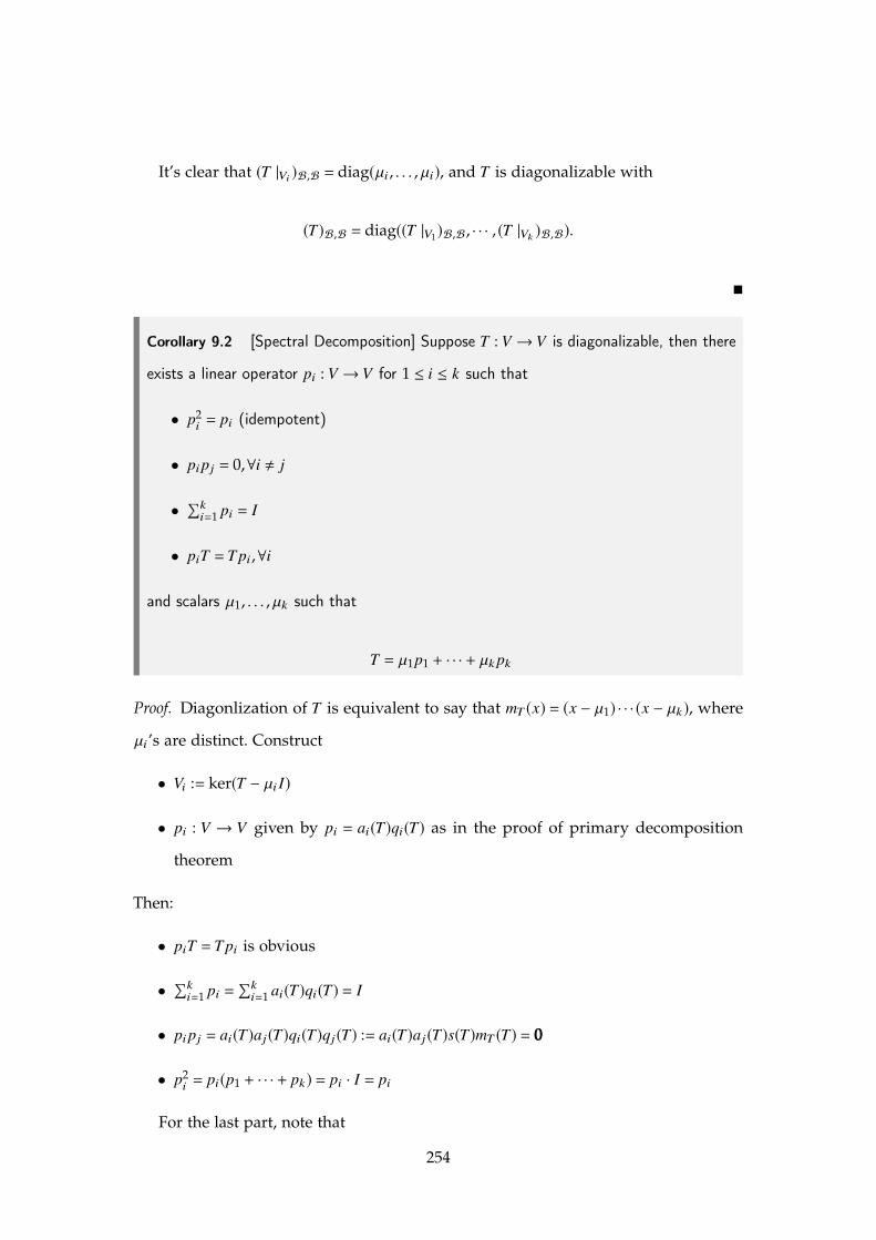
It’s clear that (T |Vi )B,B = diag(µi, . . . , µi), and T is diagonalizable with
(T)B,B = diag((T |V1)B,B , · · · , (T |Vk )B,B).
⌅
Corollary 9.2 [Spectral Decomposition] Suppose T : V ! V is diagonalizable, then there
exists a linear operator pi : V ! V for 1 i k such that
• p2i = pi (idempotent)
• pipj = 0,8i , j
•Õk
i=1 pi = I
• piT = T pi,8i
and scalars µ1, . . . , µk such that
T = µ1p1 + · · · + µkpk
Proof. Diagonlization of T is equivalent to say that mT (x) = (x � µ1) · · · (x � µk), where
µi’s are distinct. Construct
• Vi := ker(T � µi I)
• pi : V ! V given by pi = ai(T)qi(T) as in the proof of primary decomposition
theorem
Then:
• piT = T pi is obvious
•Õk
i=1 pi =Õk
i=1 ai(T)qi(T) = I
• pipj = ai(T)aj(T)qi(T)qj(T) := ai(T)aj(T)s(T)mT (T) = 000
• p2i = pi(p1 + · · · + pk) = pi · I = pi
For the last part, note that
254
• piV Vi,8i: for 8vvv 2 V ,
(T � µi I)pivvv = (T � µi I)ai(T)qi(T)vvv = ai(T)mT (x)vvv = 000
Therefore, piV ker(T � µi I) = Vi
• Now, for all www 2 V ,
Twww = T(p1 + · · · + pk)www
= T p1www + · · · +T pkwww
= (µ1p1)www + · · · + (µkpk)www
and therefore T = µ1p1 + · · · + µkpk
⌅
Organization of future two weeks. We are interested in under which condition
does the T is diagonalizable. One special case is T = A, where AAA is a symmetric matrix.
We will study normal operators, which includes the case for symmetric matrices.
Question: what happens if mT (x) contains repeated linear factors? We will spend
the next whole class to show the Jordan Normal Form:
Theorem 9.2 — Jordan Normal Form. Let F be algebraically closed field such that
every linear operator T : V ! V has the form
mT (x) =k÷i=1
(x � �i)ei
where �i’s are distinct.
Then there exists basis A of V such that
(T)A,A = diag(JJJ1, . . . , JJJk)
255

where
JJJi =
©≠≠≠≠≠≠≠≠´
µ 1 0 0
0 µ 1 0
0... . . . ...
0 0 · · · µ
™ÆÆÆÆÆÆÆƨ
for some µ 2 {�1, . . . ,�k}
256
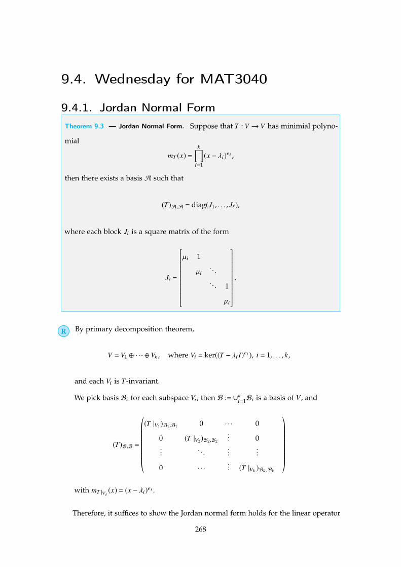
9.4. Wednesday for MAT3040
9.4.1. Jordan Normal FormTheorem 9.3 — Jordan Normal Form. Suppose that T : V ! V has minimial polyno-
mial
mT (x) =k÷i=1
(x � �i)ei ,
then there exists a basis A such that
(T)A,A = diag(J1, . . . , J`),
where each block Ji is a square matrix of the form
Ji =
2666666666664
µi 1
µi. . .. . . 1
µi
3777777777775
.
R By primary decomposition theorem,
V = V1 � · · · � Vk , where Vi = ker((T � �i I)ei ), i = 1, . . . , k,
and each Vi is T-invariant.
We pick basis Bi for each subspace Vi, then B := [ki=1Bi is a basis of V , and
(T)B,B =
©≠≠≠≠≠≠≠≠´
(T |V1)B1,B1 0 · · · 0
0 (T |V2)B2,B2
... 0... . . . ...
...
0 · · · ... (T |Vk )Bk ,Bk
™ÆÆÆÆÆÆÆƨ
with mT |Vi(x) = (x � �i)ei .
Therefore, it suffices to show the Jordan normal form holds for the linear operator
268
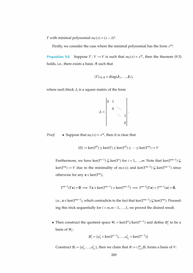
T with minimal polynomial mT (x) = (x � �)e.
Firstly, we consider the case where the minimal polynomial has the form xm:
Proposition 9.6 Suppose T : V ! V is such that mT (x) = xm, then the theorem (9.3)
holds, i.e., there exists a basis A such that
(T)A,A = diag(JJJ1, . . . , JJJ`),
where each block Ji is a square matrix of the form
Ji =
2666666666664
0 1
0 . . .. . . 1
0
3777777777775
.
Proof. • Suppose that mT (x) = xm, then it is clear that
{0} := ker(T0) ker(T) ker(T2) · · · ker(Tm) := V
Furthermore, we have ker(T i�1) $ ker(T i) for i = 1, . . . ,m: Note that ker(Tm�1) $
ker(Tm) := V due to the minimality of mT (x); and ker(Tm�2) $ ker(Tm�1) since
otherwise for any xxx 2 ker(Tm),
Tm�1(T xxx) = 000 =) T xxx 2 ker(Tm�1) = ker(Tm�2) =) Tm�2(T xxx) = Tm�1(xxx) = 000,
i.e., xxx 2 ker(Tm�1), which contradicts to the fact that ker(Tm�1) $ ker(Tm). Proceed-
ing this trick sequentially for i = m,m � 1, . . . ,1, we proved the disired result.
• Then construct the quotient space Wi = ker(T i)/ker(T i�1) and define B 0i to be a
basis of Wi:
B 0i = {ai1 + ker(T i�1), . . . ,ai`i + ker(T i�1)}
Construct Bi = {ai1, . . . ,ai`i }, then we claim that B := [mi=1Bi forms a basis of V :
269

– First proof the case m = 2 first: let U V (dim(V) <1), and B1 = {a11, . . . , a1
k1}
be a basis of U, and
B 02 = {a2
1 +U, . . . ,a2k2+U}
be a basis of V/U. Then to show the statement suffices to show that
2ÿi=1
{ai1, . . . ,aiki } forms a basis of V .
It’s clear that [2i=1{ai1, . . . ,aiki } spans V . Furthermore, dim(V) = dim(U) +
dim(V/U) = k1 + k2, i.e., [2i=1{ai1, . . . ,aiki } contains correct amount of vectors.
The proof is complete.
– This result can be extended from 2 to general m, thus the claim is shown.
• For i < m, consider the set Si = {T(www j) + ker(T i�1) | www j 2 Bi+1}. Note that
– Since T i+1(www j) = 000, T i(T(www j)) = 000, we imply T(www j) 2 ker(T i), i.e., Si ✓ Wi.
– The set Si is linearly independent: consider the equation
’j
k j(T(www j) + ker(T i�1)) = 000Wi () T
’j
k jwww j
!+ ker(T i�1) = 000Wi
i.e.,
T
’j
k jwww j
!2 ker(T i�1)() T i�1(T(
’j
k jwww j)) = 000V ,
i.e.,Õ
j k jwww j 2 ker(T i), i.e.,
’j
k jwww j + ker(T i) = 000Wi+1 ()’j
k j(www j + ker(T i)) = 000Wi+1 .
Since {www j + ker(T i), 8 j} fomrs a basis of Wi+1, we imply k j = 0,8 j.
From Bi+1 we construct Si, which is linearly independent in Wi. Therefore, we
imply |T(Bi+1)| |Bi | for 8i < m (why?).
• Now we start to construct a basis A of V :
– Start with B 0m := {um
1 +ker(Tm�1), . . . ,um`m+ker(Tm�1)}, and Bm = {um
1 , . . . ,um`m
}.
270
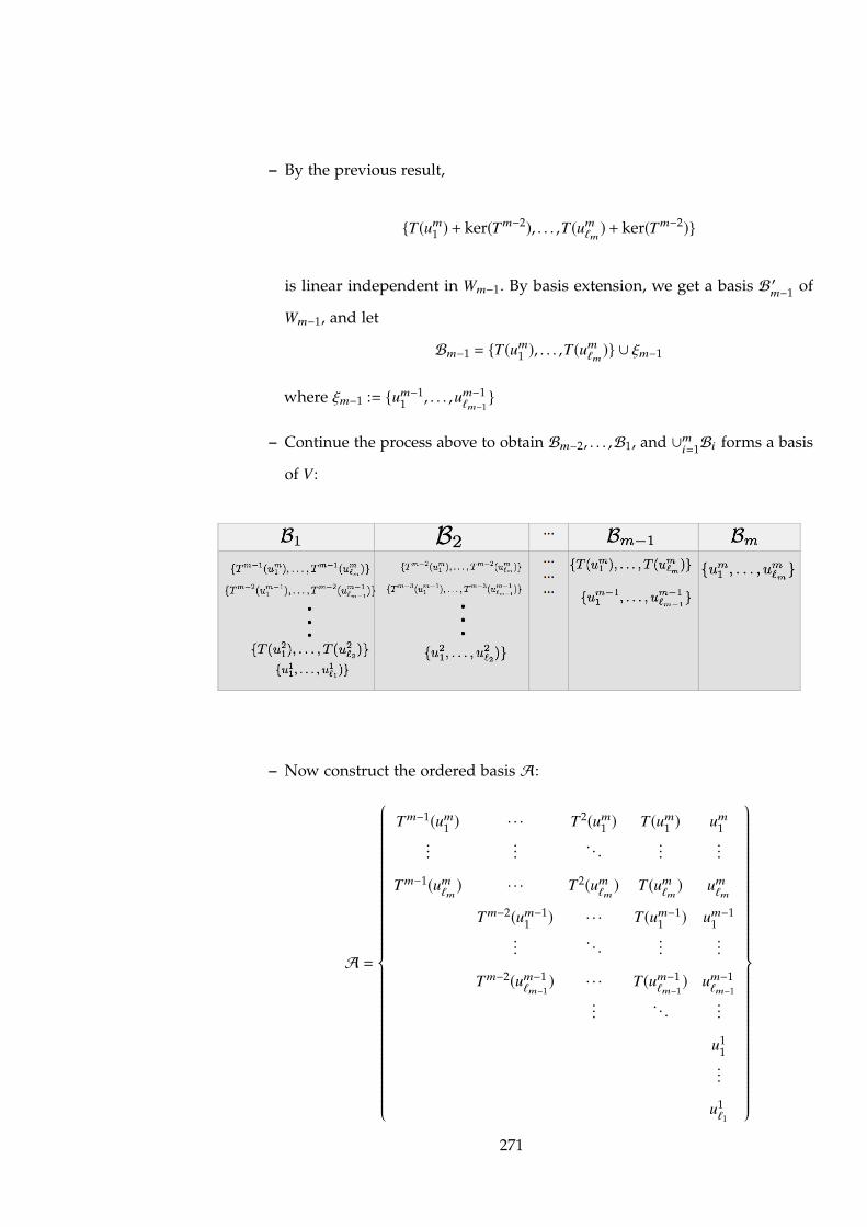
– By the previous result,
{T(um1 ) + ker(Tm�2), . . . ,T(um
`m) + ker(Tm�2)}
is linear independent in Wm�1. By basis extension, we get a basis B 0m�1 of
Wm�1, and let
Bm�1 = {T(um1 ), . . . ,T(um
`m)} [ ⇠m�1
where ⇠m�1 := {um�11 , . . . ,um�1
`m�1}
– Continue the process above to obtain Bm�2, . . . ,B1, and [mi=1Bi forms a basis
of V :
– Now construct the ordered basis A:
A =
8>>>>>>>>>>>>>>>>>>>>>>>>>>>>><>>>>>>>>>>>>>>>>>>>>>>>>>>>>>:
Tm�1(um1 ) · · · T2(um
1 ) T(um1 ) um
1...
... . . . ......
Tm�1(um`m) · · · T2(um
`m) T(um
`m) um
`m
Tm�2(um�11 ) · · · T(um�1
1 ) um�11
... . . . ......
Tm�2(um�1`m�1
) · · · T(um�1`m�1
) um�1`m�1
... . . . ...
u11...
u1`1
9>>>>>>>>>>>>>>>>>>>>>>>>>>>>>=>>>>>>>>>>>>>>>>>>>>>>>>>>>>>;
271
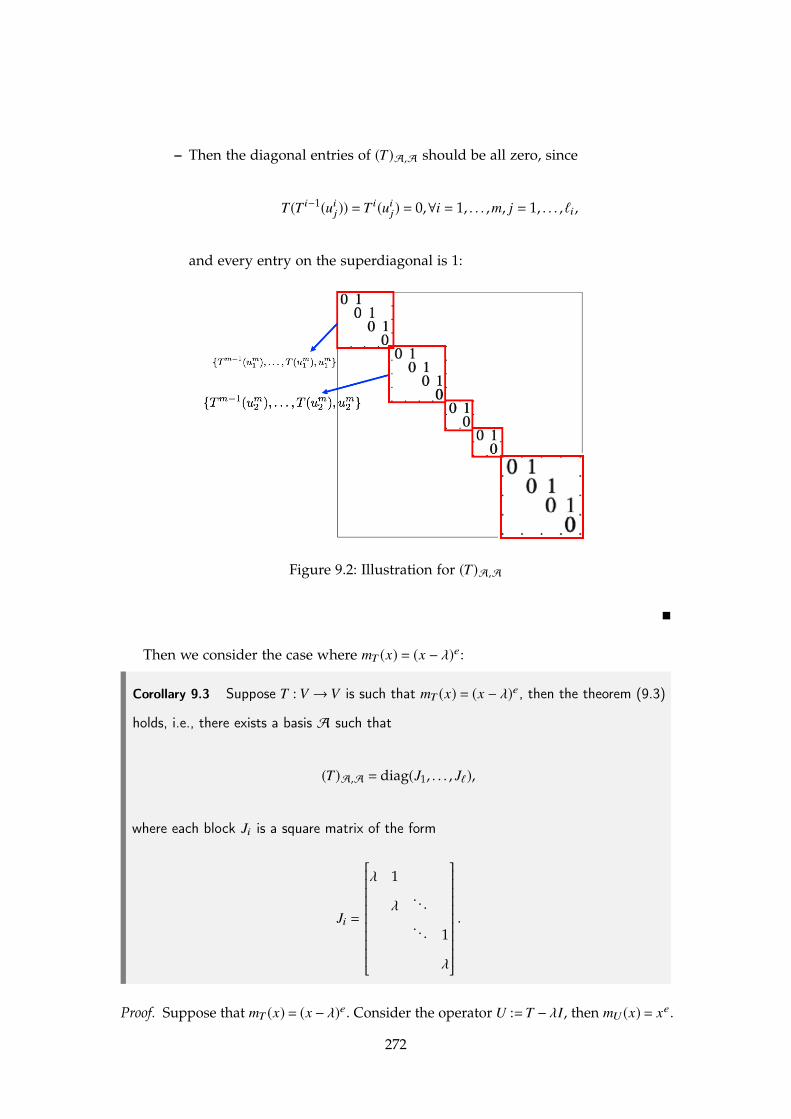
– Then the diagonal entries of (T)A,A should be all zero, since
T(T i�1(uij)) = T i(uij) = 0,8i = 1, . . . ,m, j = 1, . . . ,`i,
and every entry on the superdiagonal is 1:
Figure 9.2: Illustration for (T)A,A
⌅
Then we consider the case where mT (x) = (x � �)e:
Corollary 9.3 Suppose T : V ! V is such that mT (x) = (x � �)e, then the theorem (9.3)
holds, i.e., there exists a basis A such that
(T)A,A = diag(J1, . . . , J`),
where each block Ji is a square matrix of the form
Ji =
2666666666664
� 1
�. . .. . . 1
�
3777777777775
.
Proof. Suppose that mT (x) = (x � �)e. Consider the operator U :=T � �I, then mU (x) = xe.
272

By applying proposition (9.6),
(U)A,A = diag(JJJ1, . . . , JJJ`),
where
Ji =
2666666666664
0 1
0 . . .. . . 1
0
3777777777775
.
Or equivalently,
(T)A,A � �(I)A,A = diag(JJJ1, . . . , JJJ`)
i.e.,
(T)A,A = diag(KKK1, . . . , KKK`),
where
KKK i =
2666666666664
� 1
�. . .. . . 1
�
3777777777775⌅
R The Jordan Normal Form Theorem (9.3) follows from our arguments using
the primary decomposition.
Corollary 9.4 Any matrix A 2 Mn⇥n(C) is similar to a matrix of the Jordan normal form
diag(JJJ1, . . . , JJJ`).
9.4.2. Inner Product Spaces
273
Definition 9.8 [Bilinear] Let V be a vector space over R. A bilinear form on V is a
mapping
F : V ⇥V ! R
satisfying
1. F(uuu + vvv,www) = F(uuu,www) + F(vvv,www)
2. F(uuu,vvv + www) = F(uuu,vvv) + F(uuu,www)
3. F(�uuu,vvv) = �F(uuu,vvv) = F(uuu,�vvv)
We say
• F is symmetric if F(uuu,vvv) = F(vvv,uuu)
• F is non-degenerate if F(uuu,www) = 000 for 8uuu 2 V implies www = 0
• F is positive definite if F(vvv,vvv) > 0 for 8vvv , 000
⌅
R If F is positive-definite, then F is non-degenerate: Suppose that F(vvv,vvv) >
0,8vvv , 000. If we have F(uuu,www) = 0 for any uuu 2 V , then in particular, when uuu = www,
we imply F(www,www) = 0. By positive-definiteness, www = 000, i.e., F is non-degenerate.
274
Chapter 10
Week10
10.1. Monday for MAT3040
10.1.1. Inner Product Space• Symmetric: F(uuu,www) = F(www,uuu),8uuu,www
• Non-degenerate: F(uuu,www) = 0,8www implies uuu = 000
• Positive definite: F(vvv,vvv) > 0,8vvv , 000
Classification. When we say V be a vector space over F, we treat ↵ 2 F as a scalar.
Definition 10.1 [Sesqui-linear Form] Let V be a vector space over C. A sesquilinear
form on V is a function F : V ⇥V ! C such that
1. F(uuu + vvv,www) = F(uuu,www) + F(vvv,www)
2. F(uuu,vvv + www) = F(uuu,vvv) + F(uuu,www)
3. F(�vvv,www) = F(vvv,�www) = �F(vvv,www),8� 2 C
In this case, we say F is conjugate symmetric if
F(vvv,www) = F(www,vvv), 8vvv,www 2 V .
The definition for non-degenerateness, and positve definiteness is the same as that in
bilinear form. ⌅
R In the sesquilinear form, why there is a � shown in condition (3)?
285
Partial Answer: We want our F to be positive definite in many cases:
• Suppose that F(vvv,vvv) > 0 and we do not have � in sesquilinear form F, it
follows that
F(ivvv, ivvv) = i2F(vvv,vvv) = �F(vvv,vvv) < 0
As a result, there will be no positive bilinear form for vector space over
C.
Therefore, � is essential to guarantee that we have a positive definite form on
vector space over C, i.e.,
F(ivvv, ivvv) = iiF(vvv,vvv) = F(vvv,vvv)
⌅ Example 10.1 Consider V = Cn, and a basic sesquilinear form is the Hermitian inner
product:
F(vvv,uuu) = vvvHuuu =✓v1 · · · vn
◆ ©≠≠≠≠≠´
w1...
wn
™ÆÆÆÆƨ=
n’i=1
viwi
In this case, we do not have symmetric property F(vvv,www) = F(www,vvv) any more, instead, we
have the conjugate symmetric property F(vvv,www) = F(www,vvv). ⌅
Definition 10.2 [Inner Product] A real (complex) vector space V with a bilinear (sesquilin-
ear) form with symmetric (conjugate symmetric) and positive definite property is called
an inner product on V . Any vector space equipped with inner product is called an inner
product space. ⌅
Notation. We write h·, ·i instead of F(·, ·) to denote inner product.
Definition 10.3 [Norm] The norm of a vector vvv is kvvvk =phvvv,vvvi. ⌅
R As a result, k↵vvvk =ph↵vvv,↵vvvi =
p↵↵hvvv,vvvi =
p|↵ |2hvvv,vvvi = |↵ |kvvvk.
286

The norm is well-defined since hvvv,vvvi � 0 (positive definiteness of inner prod-
uct).
Definition 10.4 [Orthogonal] We say a family of vectors S = {vvvi | i 2 I} is orthogonal if
hvvvi,vvv ji = 0, 8i , j
If furthermore hvvvi,vvvii = 1,8i, then we say S is an orthonormal set. ⌅
R
1. The Cauchy-Scharwz inequality holds for inner product space:
|huuu,vvvi | kuuukkvvvk, 8uuu,vvv 2 V .
Proof. The proof for huuu,vvvi 2 R is the same as in MAT2040 course. Check
Theorem (6.1) in the note
https://walterbabyrudin.github.io/information/Notes/MAT2040.pdf
However, for huuu,vvvi 2 C \ R, we need the re-scaling technique:
Let www = 1huuu,vvvi
uuu, then hwww,vvvi 2 R:
hwww,vvvi = h 1huuu,vvvi
uuu,vvvi =
1huuu,vvvi
!huuu,vvvi = 1
huuu,vvvi huuu,vvvi = 1.
Applying the Cauchy-Scharwz inequality for hwww,vvvi 2 R gives
�����h1
huuu,vvviuuu,vvvi
����� = |hwww,vvvi |
kwwwkkvvvk =�����
1huuu,vvvi
uuu
����� kvvvk
Or equivalently, ���� 1huuu,vvvi
���� |huuu,vvvi | �����
1huuu,vvvi
����� kuuukkvvvk
287
Since��� 1huuu,vvvi
��� = ��� 1huuu,vvvi
���, we imply
|huuu,vvvi | kuuukkvvvk
⌅
2. The triangle inequality also holds for inner product process:
kuuu + vvvk kuuuk + kvvvk
3. The Gram-Schmidt process holds for finite set of vectors: let S = {vvv1, . . . ,vvvn}
be (finite) linearly independent. Then we can construct an orthonormal
set from S:
www1 = vvv1, wwwi+1 = vvvi+1 �hvvvi+1,www1ikwww1k2 � hvvvi+1,www2i
kwww2k2 � · · ·� hvvvi+1,wwwiikwwwi k2 , i = 1, . . . ,n�1
Then after normalization, we obtain the constructed orthonormal set.
Consequently, every finite dimensional inner product space has an
orthonormal basis.
10.1.2. Dual spaces
Theorem 10.1 — Riesz Representation. Consider the mapping
� : V ! V⇤
with vvv 7! �vvv
where �vvv(w) = hvvv,wi, 8w 2 V
Then the mapping � is well-defined and it is an R-linear transformation.
Moreover, if V is finite dimensional, then � is an isomorphism.
The R-linear transformation V ! V⇤ means that, when V ,V⇤ are vector space over
R, the R-linear transformation deduces into exactly the linear transformation.
288

R The R-linear transformation V !V⇤ is not necessarily linear if V ,V⇤ are vector
spaces over C.
However, we can transform a vector space over C into a vector space over R:
• For example, suppose that {vvv1, . . . ,vvvn} is a basis of V over C, i.e.,
vvv =n’j=1
↵jvvv j
where ↵j = pj + iqj ,8pj , qj 2 R, then
vvv =’j
pjvvv j +’j
qj(ivvv j), pj , qj 2 R
Therefore, {vvv1, . . . ,vvvn, ivvv1, . . . , ivvvn} forms a basis of V over R.
Note that ivvv1 cannot be considered as a linear combination of vvv1 over R, but
a linear combination of vvv1 over C.
In particular, if � : V ! V⇤ is a R-linear transformation, then
�(ivvv) , i�(vvv), but �(2vvv) = 2�(vvv).
Proof. 1. Well-definedness: We need to show �vvv 2 V⇤, i.e., for scalars a, b,
�vvv(awww1 + bwww2) = hvvv,awww1 + bwww2i = ahvvv,www1i + bhvvv,www2i = a�vvv(www1) + b�vvv(www2)
Therefore, �vvv 2 V⇤.
2. R-linearity of �: it suffices to show
�(cvvv1 + dvvv2) = c�(vvv1) + d�(vvv2), 8c, d 2 R,vvv1,vvv2 2 V .
For all www 2 V , we have
�cvvv1+dvvv2(www) = hcvvv1 + dvvv2,wwwi = chvvv1,wwwi + dhvvv2,wwwi = c�vvv1(www) + d�vvv2(www)
289

where the second equality holds because c, d 2 R.
Therefore,
�(cvvv1 + dvvv2) = c�(vvv1) + d�(vvv2).
⌅
290
10.4. Wednesday for MAT3040Reviewing. Consider the mapping
� : V ! V⇤
with �(vvv) = �vvvwhere �vvv(www) = hvvv,wwwi
The Riesz Representation Theorem claims that
1. � is a R-linear transformation.
2. � is injective.
3. If dim(V) <1, then � is an isomorphism.
Proof for Claim (2). Consider the equality �(vvv) = �vvv = 0V ⇤ , which implies
�vvv(www) = hvvv,wwwi = 0,8www 2 V
By the non-degenercy property, vvv = 0vvv, i.e., � is injective. ⌅
Proof for Claim (3). Since dimR(V) = dimR(V⇤), and � is injective as a R-linear transfor-
mation, we imply � is an isomorphism from V to V⇤, where V ,V⇤ are treated as vector
spaces over R. ⌅
10.4.1. Orthogonal Complement
Definition 10.5 [Orthogonal Complement] Let U V be a subspace of an inner product
space. Then the orthogonal complement of U is
U? = {vvv 2 V | hvvv,uuui = 0,8uuu 2 U}
⌅
The analysis for orthogonal complement for vector spaces over C is quite similar as
what we have studied in MAT2040.
297

Proposition 10.7 1. U? is a subspace of V
2. U \U? = {0}
3. U1 ✓ U2 implies U?2 U?
1 .
Proof. 1. Suppose that vvv1,vvv2 2 U?, where a, b 2 K (K = C or R), then for all uuu 2 U,
havvv1 + bvvv2,uuui = ahvvv1,uuui + bhvvv2,uuui
= a · 0 + b · 0 = 0
Therefore, avvv1 + bvvv2 2 U?.
2. Suppose that uuu 2 U \U?, then we imply huuu,uuui = 0. By the positive-definiteness of
inner product, uuu = 000.
3. The statement (3) is easy.
⌅
Proposition 10.8 1. If dim(V) <1 and U V , then V =U � U?
2. If U,W V , then
(U +W)? =U? \W?
(U \W)? ◆ U? +W?
(U?)? ◆ U
Moreover, if dim(V) <1, then these are equalities.
Proof. 1. Suppose that {vvv1, . . . ,vvvk} forms a basis for U, and by basis extension, we
obtain {vvv1, . . . ,vvvk ,vvvk+1, . . . ,vvvn} is a basis for V .
By Gram-Schmidt Process, any finite basis induces an orthonormal basis.
Therefore, suppose that {eee1, . . . ,eeek} forms an orthonormal basis for U, and
{eeek+1, . . . , eeen} forms an orthonormal basis for U?.
It’s easy to show V =U +U? using orthonormal basis.
2. (a) The reverse part (U +W)? ◆ U? \W? is trivial; for the forward part, suppose
298
vvv 2 (U +W)?, then
hvvv,uuu + wwwi = 0, 8uuu 2 U, www 2 W
Taking uuu ⌘ 000 in the equality above gives hvvv,wwwi = 0, i.e., vvv 2 U?. Similarly,
vvv 2 W?.
(b) Follow the similar argument as in (2a). If dim(V) <1, then write down the
orthonormal basis for U? +W? and (U \W)?.
(c) Follow the similar argument as in (2a). If dim(V) <1, then
V =U? � (U?)? =U � U?.
Therefore, (U?)? =U.
⌅
Proposition 10.9 The mapping � : V ! V⇤ maps U? V injectively to Ann(U) V⇤. If
dim(V) <1, then U? � Ann(U) as R-vector spaces
Proof. The injectivity of � has been shown at the beginning of this lecture. For any
vvv 2 U?, we imply �vvv(uuu) = 0,8uuu 2 U, i.e., �vvv 2 Ann(U).
Therefore, �(U?) Ann(U).
Provided that dim(V) <1, by (1) in proposition (10.8),
dim(U) + dim(U?) = dim(V)
Since dim(U) + dim(Ann(U)) = dim(V), we imply dim(U?) = dim(Ann(U)).
Moreover,
� : U? ! Ann(U)
is an isomorphism between R-vector spaces U? and Ann(U). ⌅
299
10.4.2. Adjoint Map
Motivation. Then we study the induced mapping based on a given linear operator
T , denoted as T 0. This induced mapping essentially plays the similar role as taking the
Hermitian for a complex matrix.
Notation. Previously we have studied the adjoint of T : V !W , denoted as T⇤ : W⇤ !
V⇤. However, from now on, we use the same terminalogy but with different meaning.
If T : V ! V is a linear operator, then the adjoint of T is the linear operator T 0 : V ! V
defined as follows.
Definition 10.6 [Adjoint] Let T : V ! V be a linear operator between inner product
spaces. The adjoint of T is defined as T 0 : V ! V satisfying
hT 0(vvv),wwwi = hvvv,T(www)i, 8www 2 V (10.1)
⌅
Proposition 10.10 If dim(V) < 1, then T 0 exists, and it is unique. Moreove, T 0 is a
linear map.
Proof. Fix any vvv 2 V . Consider the mapping
↵vvv : wwwT�! T(www) �vvv��! hvvv,T(www)i
This is a linear transformation from V to F, i.e., ↵vvv 2 V⇤
By Riesz representation theorem, � is an isomorphism from V to V⇤. Therefore, for
any ↵vvv 2 V⇤, there exists a vector T 0(vvv) 2 V such that
�(T 0(vvv)) = ↵vvv 2 V⇤
Or equivalently, �T 0(vvv)(www) = ↵vvv(www),8www 2 V , i.e., hT 0(vvv),wwwi = hvvv,T(www)i.
Therefore, from vvv we have constructed T 0(vvv) satisfying (10.1). Now define T 0 : V !V
by vvv 7! T 0(vvv).
300

• Since the choice of T 0(vvv) is unique by the injectivity of �, T 0 is well-defined.
• Now we show T 0 is a linear transformation: Let vvv1,vvv2 2 V ,a, b 2 K . For all www 2 V ,
we have
hT 0(avvv1 + bvvv2),wwwi = havvv1 + bvvv2,T(www)i
= ahvvv1,T(www)i + bhvvv2,T(www)i
= ahT 0(vvv1),wwwi + bhT 0(vvv2),wwwi
= haT 0(vvv1) + bT 0(vvv2),wwwi
Therfore,
hT 0(avvv1 + bvvv2) � [aT 0(vvv1) + bT 0(vvv2)],wwwi = 0, 8www 2 V
By the non-degeneracy of inner product,
T 0(avvv1 + bvvv2) � [aT 0(vvv1) + bT 0(vvv2)] = 000,
i.e., T 0(avvv1 + bvvv2) = aT 0(vvv1) + bT 0(vvv2)
⌅
⌅ Example 10.2 Let V = Rn, h·, ·i as the usual inner product. Consider the matrix-
multiplication mapping
T : V ! V
T(vvv) = Avvv
Then hT 0(vvv),wwwi = hvvv,T(www)i implies
(T 0(vvv))Twww = hvvv, AAAwwwi
= vvvT AAAwww
= (AAATvvv)Twww
Therfore, T 0(vvv) = ATvvv. ⌅
301

Proposition 10.11 Let T : V ! V be a linear transformation, V a inner product space.
Suppose that B = {eee1, . . . , eeen} is an orthonormal basis of V , then
(T 0)B,B = ((T)B,B)T
Proof. Suppose that (T)B,B = (ai j), where T(eee j) =Õn
k=1 ak jeeek , then
heeei,T(eee j)i = heeei,n’
k=1
ak jeeeki
=
n’k=1
ak j heeei, eeeki
= ai j
Also, suppose (T 0)B,B = (bi j), we imply T 0(eee j) =Õn
k=1 bi jeeek , which follows that
heeei,T 0(eee j)i = bi j =) hT 0(eee j), eeeii = bi j =) heee j ,T(eeei)i = bi j ,
i.e., aji = bi j . ⌅
R Proposition (10.11) does not hold if B is not an orthonormal basis.
302
Chapter 11
Week11
11.1. Monday for MAT3040Reviewing. Adjoint Operator: hT 0(vvv),wwwi = hvvv,T(www)i.
11.1.1. Self-Adjoint Operator
Definition 11.1 [Self-Adjoint] Let V be an inner product space and T : V !V be a linear
operator. Then T is self-adjoint if T 0 = T . ⌅
⌅ Example 11.1 Let V =Cn, and B = {eee1, . . . , eeen} be a orthonormal basis. Let T : V !V
be given by
T(vvv) = AAAvvv, where A 2 Mn⇥n(C).
Or equivalently, there exists basis B such that (T)B,B = AAA.
In such case, T is self-adjoint if and only if (T 0)B,B = (T)B,B , i.e., (T)TB,B = (T)B,B , i.e.,
AAAH = AAA.
Therefore, T(vvv) = AAAvvv is self-adjoint if and only if AAAH = AAA.
Moreover, if C is replaced by R, then T is seld-adjoint if and only if AAA is symmetric. ⌅
R The notion of self-adjoint for linear operator is essentially the generalized
notion of Hermitian for matrix that we have stuided in MAT2040.
We also have some nice properties for self-adjoint, and the proof for which are
essentially the same for the proof in the case of Hermitian matrices.
315

Proposition 11.1 If � is an eigenvalue of a self-adjoint operator T , then � 2 R.
Proof. Suppose there is an eigen-pair (�,www) for www , 000, then
�hwww,wwwi = hwww,�wwwi
= hwww,T(www)i = hT 0(www),wwwi
= hT(www),wwwi = h�www,wwwi
= �hwww,wwwi
Since hwww,wwwi , 0 by non-degeneracy property, we have � = �, i.e., � 2 R. ⌅
Proposition 11.2 If U V is T-invariant over the self-adjoint operator T , then so is U?.
Proof. It suffices to show T(vvv) 2 U?,8vvv 2 U?, i.e., for any uuu 2 U, check that
huuu,T(vvv)i = hT 0(uuu),vvvi = hT(uuu),vvvi = 0,
where the last equality is because that T(uuu) 2 U and vvv 2 U?. Therefore, T(vvv) 2 U?. ⌅
Theorem 11.1 If T : V ! V is self-adjoint, and dim(V) < 1, then there exists an
orthonormal basis of eigenvectors of T , i.e., an orthonormal basis of V such that any
element from this basis is an eigenvector of T .
Proof. We use the induction on dim(V):
• The result is trival for dim(V) = 1.
• Suppose that this theorem holds for all vector spaces V with dim(V) k, then we
want to show the theorem holds when dim(V) = k + 1:
Suppose that T : V ! V is self-adjoint with dim(V) = k + 1, then consider
XT (x) = xk+1 + · · · + a1x + a0, ai 2 K, where K denotes R or C.
316

– If K = C, then XT (x) can be decomposed as
XT (x) = (x � �1) · · · (x � �k+1)
In paricular, we obtain the eigen-pair (�1,vvv)
– If K =R, i.e., we treat real number as scalars, then
XT (x) = (x � �1) · · · (x � �k+1), where �i 2 C.
By proposition (11.1), we imply all �i’s are in R. Moreover, we also obtain
the eigen-pair (�1,vvv)
Consider U = span{vvv}, then
– U is T-invariant
– V =U � U?, since V is finite dimensional
– U? is T-invariant.
Consider T |U? , which is a self-adjoint operator on U?, with dim(U?) = k.
By induction, there exists an orthonormal basis {eee2, . . . , eeek+1} of eigenvectors of
T |U? .
Consider the basis B = {vvv0 = vvv/kvvvk, eee2, . . . , eeek+1}. As a result,
1. B forms a basis of V
2. All vvv0, eeei are of norm 1 eigenvectors of T .
3. B is an orthonormal set, e.g., hvvv0, eeeii = 0, where vvv0 2 U and eeei 2 U?.
Therefore, B is a basis of orthonormal eigenvectors of V .
⌅
Corollary 11.1 If dim(V) <1, and T : V !V is self-adjoint, then there exists orthonormal
basis B such that
(T)B,B = diag(�1, . . . ,�n)
317
In paticular, for all real symmtric matrix AAA 2 Sn, there exists orthogonal matrix P (PTP = IIIn)
such that
P�1 AP = diag(�1, . . . ,�n)
Proof. 1. By applying theorem (11.1), there exists orthonormal basis of V , say B =
{vvv1, . . . ,vvvn} such that T(vvvi) = �ivvvi. Directly writing the basis representation gives
(T)B,B = diag(�1, . . . ,�n).
2. For the second part, consider T : Rn ! R
n by T(vvv) = AAAvvv. Since AAAT = AAA, we imply
T is self-adjoint. There exists orthonormal basis B = {vvv1, . . . ,vvvn} such that
(T)B,B = diag(�1, . . . ,�n).
In particular, if A = {eee1, . . . , eeen}, then (T)A,A = AAA. We construct P := CA,B , which
is the change of basis matrix from B to A, then
P =✓vvv1 · · · vvvn
◆
and
P�1(T)A,AP = (T)B,B
Or equivalently, P�1 AP = diag(�1, . . . ,�n), with
PTP =
©≠≠≠≠≠´
vvvT1...
vvvTn
™ÆÆÆÆƨ
✓vvv1 · · · vvvn
◆= III
⌅
11.1.2. Orthononal/Unitary Operators
318

Definition 11.2 A linear operator T : V !V over K with hT(www),T(vvv)i = hwww,vvvi,8vvv,www 2 V ,
is called
1. Orthogonal if K =R
2. Unitary if K = C
⌅
Proposition 11.3 T is orthogonal / unitary if and only if T 0 �T = I
Proof. The reverse direction is by directly checking that
hT(www),T(vvv)i = hT 0 �T(www),vvvi = hwww,vvvi
The forward direction is by checking T 0 �T(www) = www,8www 2 V :
hT 0 �T(www),vvvi = hT(www),T(vvv)i = hwww,vvvi =) hT 0 �T(www) � www,vvvi = 0,8vvv 2 V
By non-degeneracy, T 0 �T(www) � www = 0, i.e., T 0 �T(www) = www,8www 2 V . ⌅
⌅ Example 11.2 Let T : Kn ! K
n be given by T(vvv) = Avvv. Then T is orthogonal implies
(T 0)B,B(T)B,B = I.
(Orthogonal) When K =R, then AT A = I
(Unitary) When K = C, then AH A = I. ⌅
Definition 11.3 [Orthogonal/Unitary Group]
Orthognoal Group : O(n,R) = {A 2 Mn⇥n(R) | AT A = I}
Unitary Group : U(n,C) = {A 2 Mn⇥n(C) | AH A = I}
⌅
319

11.4. Wednesday for MAT3040Reviewing. Unitary Operators
hTvvv,Twwwi = hvvv,wwwi, 8vvv,www 2 V .
11.4.1. Unitary Operator
⌅ Example 11.8 Let V =Rn with usual inner product. For the linear operator T(vvv) = AAAvvv,
T is orthogonal if and only if AAAT AAA = III.
Let V = Cn with usual inner product. For the linear operator T(vvv) = AAAvvv, T is unitary if
and only if AAAH AAA = III. ⌅
Proposition 11.8 Let T : V !V be a linear operator on a vector space over K satisfying
T 0T = I. Then for all eigenvalues � of T , we have |� | = 1.
Proof. Suppose we have the eigen-pair (�,vvv), then
hTvvv,Tvvvi = hvvv,vvvi
() h�vvv,�vvvi = hvvv,vvvi
() ��hvvv,vvvi = hvvv,vvvi
Since hvvv,vvvi , 0 (vvv , 000), we imply |� |2 = 1, i.e., |� | = 1. ⌅
Proposition 11.9 Let T : V !V be an operator on a finite dimension V over K satisfying
T 0T = I. If U V is T-invariant, then U is also T�1-invariant.
Proof. Since T 0T = I, i.e., T is invertible, we imply 0 is not a root of XT (x), i.e., 0 is not a
root of mT (x). Since mT (0) , 0, mT (x) has the form
mT (x) = xm + · · · + a1x + a0, a0 , 0,
332
which follows that
mT (T) = Tm + · · · + a0I = 0 =) T(Tm�1 + · · · + a1I) = �a0I
Or equivalently,
T✓� 1
a0(Tm�1 + · · · + a1I)
◆= I
Therefore,
T�1 = � 1a0
Tm�1 � · · · � a2
a0T � a1
a0I,
i.e., the inverse T�1 can be expressed as a polynomial involving T only.
Sicne U is T-invariant, we imply U is Tm-invariant for m 2 N, and therefore U is
T�1-invariant since T�1 is a polynomial of T . ⌅
Proposition 11.10 Let T : V !V satisfies T 0T = I (dim(V) <1), then U V is T-invariant
implies U? is T-invariant.
Proof. Let v 2 U?, it suffices to show T(v) 2 U?.
For all u 2 U, we have
hu,T(v)i = hT 0(u),vi = hT�1(u),vi
Since U is T�1-invaraint, we imply T�1(u) 2 U, and therefore
hu,T(v)i = hT�1(u),vi = 0 =) T(v) 2 U?.
⌅
Theorem 11.2 Let T : V ! V be a unitary operator on finite dimension V (over C),
then there exists an orthonormal basis A such that
(T)A,A = diag(�1, . . . ,�n), |�i | = 1, 8i.
Proof Outline. Note that XT (x) always admits a root in C, so we can always find an
333
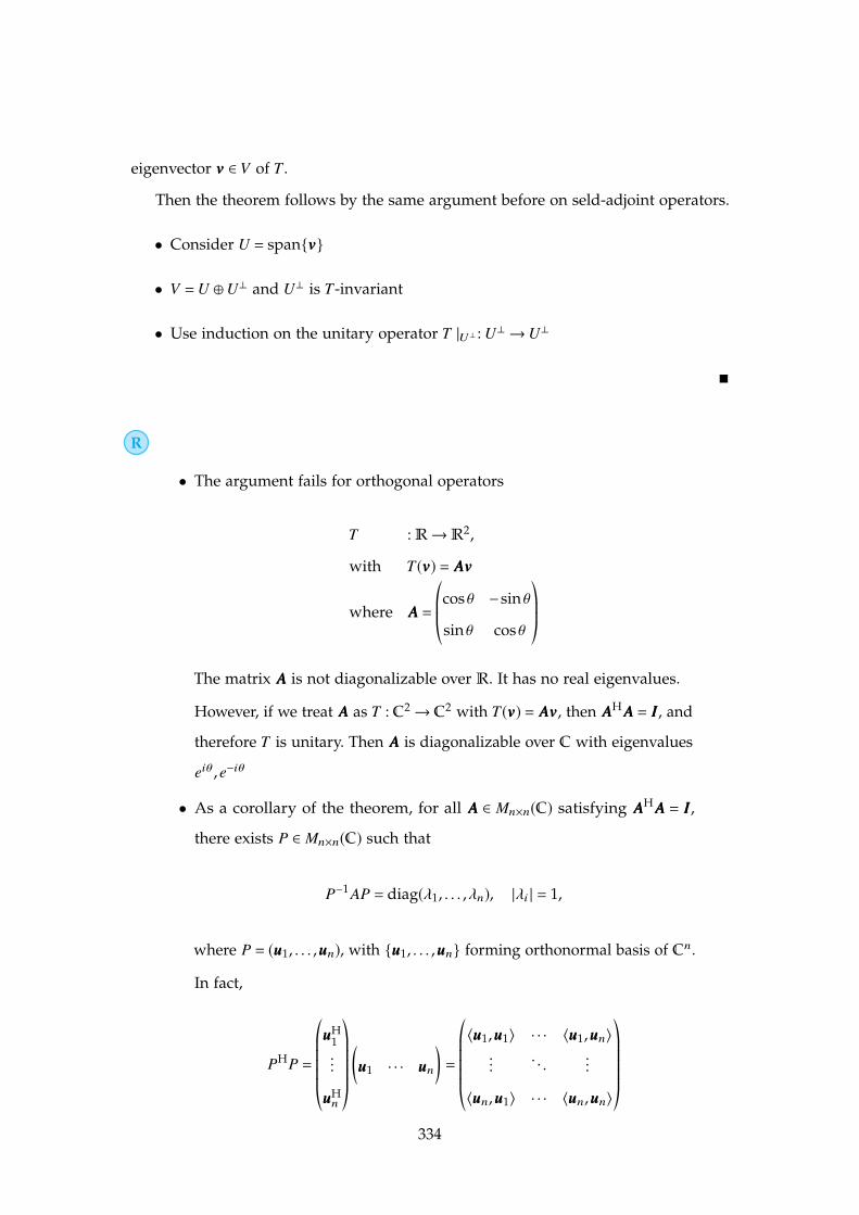
eigenvector vvv 2 V of T .
Then the theorem follows by the same argument before on seld-adjoint operators.
• Consider U = span{vvv}
• V =U � U? and U? is T-invariant
• Use induction on the unitary operator T |U? : U? ! U?
⌅
R
• The argument fails for orthogonal operators
T : R ! R2,
with T(vvv) = AAAvvv
where AAA =©≠≠´cos✓ �sin✓
sin✓ cos✓
™Æƨ
The matrix AAA is not diagonalizable over R. It has no real eigenvalues.
However, if we treat AAA as T : C2 ! C
2 with T(vvv) = AAAvvv, then AAAH AAA = III, and
therefore T is unitary. Then AAA is diagonalizable over C with eigenvalues
ei✓ , e�i✓
• As a corollary of the theorem, for all AAA 2 Mn⇥n(C) satisfying AAAH AAA = III,
there exists P 2 Mn⇥n(C) such that
P�1 AP = diag(�1, . . . ,�n), |�i | = 1,
where P = (uuu1, . . . ,uuun), with {uuu1, . . . ,uuun} forming orthonormal basis of Cn.
In fact,
PHP =
©≠≠≠≠≠´
uuuH1...
uuuHn
™ÆÆÆÆƨ
✓uuu1 · · · uuun
◆=
©≠≠≠≠≠´
huuu1,uuu1i · · · huuu1,uuuni... . . . ...
huuun,uuu1i · · · huuun,uuuni
™ÆÆÆÆƨ
334
Conclusion: all matrices AAA 2 Mn⇥n(C) with AAAH AAA = III can be written as
AAA = PPP�1 diag(�1, . . . ,�n)PPP,
with some PPP satisfying PPPHPPP = III.
Notation. Let U(n) = {AAA 2 Mn⇥n(C) | AAAH AAA = III)} be the unitary group, then all AAA 2 U(n)
can be diagonalized by
A = P�1 diag(�1, . . . ,�n)P, P 2 U(n).
11.4.2. Normal Operators
Definition 11.10 [Normal] Let T : V ! V be a linear operator over a C inner product
vector space V . We say T is normal, if
T 0T = TT 0
⌅
⌅ Example 11.9 • All self-adjoint operators are normal:
T = T 0 =) TT 0 = T 0T = T2
• All (finite-dimensional) unitary operators are normal:
T 0T = TT 0 = I
⌅
Proposition 11.11 Let T be a normal operator on V . Then
1. kT(vvv)k = kT 0(vvv)k,8vvv 2 V .
In particular, T(vvv) = 0 if and only if T 0(vvv) = 0
335
2. (T � �I) is also a normal operator, for any � 2 C
3. T(vvv) = �vvv if and only if T 0(vvv) = �vvv.
Proof. 1.
hTvvv,Tvvvi = hT 0Tvvv,vvvi
= hTT 0vvv,vvvi
= hvvv,TT 0vvvi
= hT 0vvv,T 0vvvi
= hT 0vvv,T 0vvvi
Therefore, kT(vvv)k2 = kT 0(vvv)k2, i.e., kT(vvv)k = kT 0(vvv)k.
2. By hw4, (T � �I)0 = T 0 � �I. It suffices to check
(T � �I)0(T � �I) = (T � �I)(T � �I)0,
Expanding both sides out gives the desired result, i.e.,
(T � �I)0(T � �I) = (T 0 � �I)(T � �I) = T 0T � �T � �T 0 + ��I
and
(T � �I)(T � �I)0 = (T � �I)(T 0 � �I) = TT 0 � �T � �T 0 + ��I
3. The proof for (3) will be discussed in the next lecture.
⌅
336

Chapter 12
Week12
12.1. Monday for MAT3040
12.1.1. Remarks on Normal OperatorProposition 12.1 If T is normal, then
1. kT(vvv)k = kT 0(vvv)k for any vvv 2 V
2. (T � �I) is normal for any � 2 C
3. T(vvv) = �vvv if and only if T 0(vvv) = �vvv
4. If T(vvv) = �vvv and T(www) = µwww with � , µ, then hvvv,wwwi = 0.
Proof. (3) • For the forward direction, if (T � �I)vvv = 0, then by part (2), (T � �I) is
normal, which follows that
k(T � �I)0(vvv)k = 0 =) (T � �I)0(vvv) = 0 =) T 0vvv = �vvv.
• For the reverse direction, suppose that (T 0 � �I)vvv = 0. Since T is normal, we
imply T 0 is normal. Then by part (2), (T 0 � �I) is normal. By applying the
same trick,
(T 0 � �I)0vvv = 0 =) ((T 0)0 � �I)vvv = 0.
By hw4, (T 0)0 = T . Therefore, (T � �I)vvv = 0.
(4) Observe that
�hvvv,wwwi = h�vvv,wwwiby (3)====) �hvvv,wwwi = hT 0(vvv),wwwi = hvvv,T(www)i = hvvv, µwwwi = µhvvv,wwwi
349
Since � , µ, we imply hvvv,wwwi = 0. The proof is complete.
⌅
Theorem 12.1 Let T be an operator on a finite dimensional (dim(V) = n) C-inner
product vector space V satisfying T 0T = TT 0. Then there is an orthonormal basis of
eigenvectors of V , i.e., an orthonormal basis of V such that any element from this
basis is an eigenvector of T .
Proof. Since XT (x) must have a root in C, there must exist an eigen-pair (vvv,�) of T .
• Construct U = span{vvv}, and it follows that
Tvvv = �vvv =) U is T-invariant.
T 0vvv = �vvv =) U is T ’-invariant.
• Moreover, we claim that U? is T and T 0 invariant: let www 2 U?, and for all uuu 2 U,
we have
huuu,T(www)i = hT 0(uuu),wwwi = h�uuu,wwwi = �huuu,wwwi = 0,
i.e., U? is T invariant.
huuu,T 0(www)i = hT(uuu),wwwi = h�uuu,wwwi = �huuu,wwwi = 0,
which implies U? is T 0 invariant.
• Therefore, we construct the operator T |U? : U? ! U?, and
TT 0 = T 0T =) (T |U?)(T 0 |U?) = (T 0 |U?)(T |U?),
i.e., (T |U?) is normal on U?. Moreover, dim(U?) = n � 1.
• Applying the same trick as in Theorem (11.1), we imply there exists an orthonor-
350
mal basis {eee2, . . . , eeen} of eigenvectors of (T |U?). Then we can argue that
B = {vvv0 = vvv/kvvvk, eee2, . . . , eeek+1}
is a basis of orthonormal eigenvectors of V .
⌅
Corollary 12.1 [Spectral Theorem for Normal Operator] Let T : V ! V be a normal
operator on a C-inner product space with dim(V) < 1. Then there exists self-adjoint
operators P1, . . . , Pk such that
P2i = Pi, PiPj = 0, i , j,
k’i=1
Pi = I,
and T =Õk
i=1 �iPi, where �i’s are the eigenvalues of T .
R These Pi’s are the orthogonal projections from V to the �i-eigenspace ker(T �
�i I) of T , i.e.,we have
v = Pi(v) + (v � Pi(v)),
where Pi(v) 2 ker(T � �i I), and v � Pi(v) 2 (ker(T � �i I))?.
You should know how to compute Pi’s when T(vvv)= AAAvvv in the course MAT2040.
Proof. Since T has a basis of eigenvectors, by definition, T is diagonalizable. By propo-
sition (8.2),
mT (x) = (x � �1) · · · (x � �k),
where �i’s are distinct. By spectral decomposition corollary (9.2), it suffices to show
Pi’s are self-disjoint.
• Recall that Pi = ai(T)qi(T) := bmTm + · · · + b1T + b0T , i.e., a polynomial of T , and
therefore
P0i = bm(T 0)m + · · · + b1(T 0) + b0I.
351

We claim that Pi is normal: Since T 0T = TT 0, we imply
(T 0)pTq = Tq(T 0)p,8p, q 2 N
which follows that
PiP0i = (bmTm + · · · + b0I)(bm(T 0)m + · · · + b1(T 0) + b0I)
=’
1x,ymbx by(T)x(T 0)y
=’
1x,ymbybx(T 0)y(T)x
= (bm(T 0)m + · · · + b1(T 0) + b0I)(bmTm + · · · + b0I)
= P0i Pi
• In general, S is self-adjoint, which implies S is normal, but not vice versa. How-
ever, the converse holds if further all eigenvalues of S are real numbers:
By Theorem (12.1), we imply S is orthonormally diagonalizable, and its diagonal
representation is of the form
(S)B,B = diag(�1, . . . ,�k).
Note that B is also a basis for S0 and elements of B are eigenvalues of S0, by
part (3) in proposition (12.1). Therefore,
(S0)B,B = diag(�1, . . . ,�k).
Therefore, S = S0.
In particular, for S = Pi, we can easily show all eigenvalues of Pi are 0 or 1, which are
real. Therefore, Pi’s are self-adjoint. ⌅
352
Corollary 12.2 Let T : V ! V be a linear operator on C-inner product space with
dim(V) <1. Then T is normal if and only if T 0 = f (T) for some polynomial f (x) 2 C[x].
Proof. • For the reverse direction, if T 0 = f (T), then T 0T = f (T)T = T f (T) = TT 0.
• For the forward direction, suppose that T is normal, then by corollary (12.1),
T =k’i=1
�iPi, Pi = fi(T), where Pi’s are self-adjoint,
which follows that
T 0 =
k’i=1
�iPi
! 0=
k’i=1
�iP0i =
k’i=1
�iPi =
k’i=1
�i fi(T)
⌅
R The normal operator is a generalization of Hermitian matrices, and it inherits
many nice properties of Hermitian.
12.1.2. Tensor ProductMotivation. Let U,V ,W be vector spaces. We want to study bilinear maps f : U ⇥W !
U, i.e.,
f (av1 + bv2,w) = a f (v1,w) + b f (v2,w)
f (v,cw1 + dw2) = c f (v,w1) + df (v,w2)
Unfortunately, bilinear form usually is not a linear transformation!
⌅ Example 12.1 • Let f : Rn ⇥ R
n ! R be with (u,v) 7! hu,vi.
• Let f : Mn⇥n(F) ⇥ Mn⇥n(F)! Mn⇥n(F) be with f (A, B) = AB.
• Let f : F[x] ⇥ F[x]! F be with f (p(x), q(x)) = p(1)q(2)
353
• Let f : F[x] ⇥ F[x]! F[x] be with f (p(x), q(x)) = p(x)q(x).
⌅
354
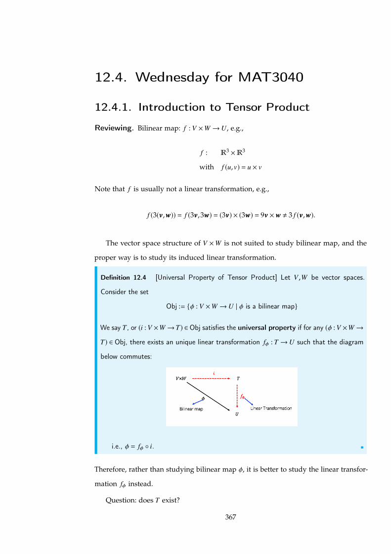
12.4. Wednesday for MAT3040
12.4.1. Introduction to Tensor Product
Reviewing. Bilinear map: f : V ⇥W ! U, e.g.,
f : R3 ⇥ R
3
with f (u,v) = u ⇥ v
Note that f is usually not a linear transformation, e.g.,
f (3(vvv,www)) = f (3vvv,3www) = (3vvv) ⇥ (3www) = 9vvv ⇥ www , 3 f (vvv,www).
The vector space structure of V ⇥W is not suited to study bilinear map, and the
proper way is to study its induced linear transformation.
Definition 12.4 [Universal Property of Tensor Product] Let V ,W be vector spaces.
Consider the set
Obj := {� : V ⇥W ! U | � is a bilinear map}
We say T , or (i : V ⇥W !T) 2 Obj satisfies the universal property if for any (� : V ⇥W !
T) 2 Obj, there exists an unique linear transformation f� : T ! U such that the diagram
below commutes:
i.e., � = f� � i. ⌅
Therefore, rather than studying bilinear map �, it is better to study the linear transfor-
mation f� instead.
Question: does T exist?
367

Definition 12.5 [Spanning Set] Let V ,W be vector spaces. Let S = {(vvv,www) | vvv 2 V ,www 2 W},
then we define
X = span(S).
⌅
R
1. The spanning set X is not addictive, e.g., x1 = 3(0,www) 2 X and x2 = 1(0,www)+
1(0,2www) 2 X, but x1 , x2.
2. Note that we assume no relations on the elements (vvv,www) 2 S. More
precisely, the set S = {(vvv,www) | vvv 2 V ,www 2 W} is linearly independent in X.
For example, (0,www) ? (0,2www).
3. The only legitimate relationship is
2(vvv1,www1) + 3(vvv1,www1) = 5(vvv,www),
which is not equal to (5vvv,5www)
4. S is a basis of X, and therefore X is of uncountable dimension.
Definition 12.6 [Special subspace of X] Let y X be a vector subspace spanned by
vectors of the form
{1(vvv1,vvv2,www) � 1(vvv1,www) � 1(vvv2,www)}, and {1(vvv,www1 + www2) � 1(vvv,www1) � 1(vvv,www2)}
and
{1(kvvv,www) � k(vvv,www) | k 2 F}
and
{1(vvv, kwww) � k(vvv,www) | k 2 F}
⌅
368

Definition 12.7 [Tensor Product] We define the tensor product V ⌦ W by
V ⌦ W = X/y.
Therefore, vvv ⌦ www = (vvv,www) + y 2 X/y ⌅
R
1. As a result, the tensor product is finitely addictive:
(vvv1 + vvv2) ⌦ www = (vvv1 + vvv2,www) + y
= (vvv1 + vvv2,www) � [(vvv1 + vvv2,www) � (vvv1,www) � (vvv2,www)] + y
= 0(vvv1 + vvv2,www) + (vvv1,www) + (vvv2,www) + y
= [(vvv1,www) + y] + [(vvv2,www) + y]
= vvv1 ⌦ www + vvv2 ⌦ www
Similarly,
vvv ⌦ (www1 + www2) = (vvv ⌦ www1) + (vvv ⌦ www2)
(kvvv) ⌦ www = k(vvv ⌦ www)
vvv ⌦ (kwww) = k(vvv ⌦ www)
2. The product space V ⇥ W is different from the tensor product space
V ⌦ W :
(a) (vvv,000) , 000V⇥W in V ⇥W ; but vvv ⌦ 0 2 0V ⌦W :
V ⌦ 0 = V ⌦ (0www)
= 0(V ⌦ w)
= 0V ⌦W
Moreover, f is bilinear implies f (vvv,0) = 000.
369
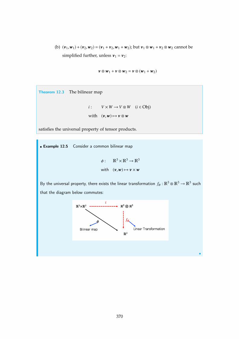
(b) (vvv1,www1)+ (vvv2,www2) = (vvv1 + vvv2,www1 +www2); but vvv1 ⌦ www1 + vvv2 ⌦ www2 cannot be
simplified further, unless vvv1 = vvv2:
vvv ⌦ www1 + vvv ⌦ www2 = vvv ⌦ (www1 + www2)
Theorem 12.3 The bilinear map
i : V ⇥W ! V ⌦ W (i 2 Obj)
with (vvv,www) 7! vvv ⌦ www
satisfies the universal property of tensor products.
⌅ Example 12.5 Consider a common bilinear map
� : R3 ⇥ R
3 ! R3
with (vvv,www) 7! vvv ⇥ www
By the universal property, there exists the linear transformation f� : R3 ⌦ R
3 ! R3 such
that the diagram below commutes:
⌅
370

Chapter 13
Week13
13.1. Monday for MAT3040
Reviewing.
1. Define S = {(vvv,www) | vvv 2 V ,www 2 W} and X = span(S). In X, there are no relations
between distinct elements of S, e.g.,
2(vvv,0) + 3(0,www) , 1(2vvv,3www)
General element in X:
a1(vvv1,www1) + · · · + an(vvvn,wwwn),
where (vvvi,wwwi) are distinct.
2. Define the space V ⌦ W = X/y, with
vvv ⌦ www = 1(vvv,www) + y 2 V ⌦ W .
General element in X/y := V ⌦ W :
a1(vvv1,www1) + · · · + an(vvvn,wwwn) + y = a1((vvv1,www1) + y) + · · · + an((vvvn,wwwn) + y)
= a1(vvv1 ⌦ www1) + · · · + an(vvvn ⌦ wwwn)
= (a1vvv1) ⌦ www1 + · · · + (anvvvn) ⌦ wwwn
381

Therefore, a general element in V ⌦ W is of the form
vvv01 ⌦ www1 + · · · + vvv0n ⌦ wwwn, vvv0i 2 V ,wwwi 2 W . (13.1)
Note that V ⌦ W is different from V ⇥ W , where all elements in V ⇥ W can be
expressed as (vvv,www).
3. The tensor product mapping
i : V ⇥W ! V ⌦ W
with (vvv,www) 7! vvv ⌦ www
satisfies the universal property.
Here we present an example for computing tensor product by making use of the
rules below:
(vvv1 + vvv2) ⌦ www = vvv1 ⌦ www + vvv2 ⌦ www
vvv ⌦ (www1 + www2) = (vvv ⌦ www1) + (vvv ⌦ www2)
(kvvv) ⌦ www = k(vvv ⌦ www)
vvv ⌦ (kwww) = k(vvv ⌦ www)
⌅ Example 13.1 Let V =W =R2, with
eee1 =©≠≠´1
0
™Æƨ
, eee2 =©≠≠´0
1
™Æƨ
.
382

Here we have
©≠≠´3
1
™Æƨ⌦
©≠≠´�4
2
™Æƨ= (3eee1 + 2eee2) ⌦ (�4eee1 + 2eee2)
= (3eee1) ⌦ (�4eee1 + 2eee2) + (eee2) ⌦ (�4eee1 + 2eee2)
= (3eee1) ⌦ (�4eee1) + (3eee1) ⌦ (2eee2) + (eee2) ⌦ (�4eee1) + eee2 ⌦ (2eee2)
= �12(eee1 ⌦ eee1) + 6(eee1 ⌦ eee2) � 4(eee2 ⌦ eee1) + 2(eee2 ⌦ eee2)
⌅
Exercise: Check that eee1 ⌦ eee2 + eee2 ⌦ eee1 cannot be re-written as
(aeee1 + beee2) ⌦ (ceee1 + deee2), a, b,c, d 2 R.
13.1.1. Basis of V ⌦ W
Motivation. Given that {vvv1, . . . ,vvvn} is a basis of V , and {www1, . . . ,wwwm} a basis of W , we
aim to find a basis of V ⌦ W using vvvi’s and wwwi’s.
Proposition 13.1 The set {vvvi ⌦ www j | 1 i n, 1 j m} spans the tensor product space
V ⌦ W .
Proof. Consider any vvv 2 V and www 2 W , and we want to express vvv ⌦ www in terms of vvvi,www j .
Suppose that vvv = ↵1vvv1 + · · · + ↵nvvvn and www = �1www1 + · · · + �mwwwm.
Substituting vvv = ↵1vvv1 + · · · + ↵nvvvn into the expression vvv ⌦ www, we imply
vvv ⌦ www = (↵1vvv1 + · · · + ↵nvvvn) ⌦ www
= (↵1vvv1) ⌦ www1 + · · · + (↵nvvvn) ⌦ wwwn
= ↵1(vvv1 ⌦ www) + · · · + ↵n(vvvn ⌦ www)
For each vvvi ⌦ www, i = 1, . . . ,n, similarly,
vvvi ⌦ www = �1(vvvi ⌦ www1) + · · · + �m(vvvi ⌦ wwwm).
383

Therefore,
vvv ⌦ www =n’i=1
m’j=1
↵i�j(vvvi ⌦ www j) (13.2)
By (13.4), any vector in V ⌦ W is of the form
vvv(1) ⌦ www(1) + · · · + vvv(`) ⌦ www(`)
By (13.5), each vvv(k) ⌦ www(k), k = 1, . . . ,`, can be expressed as
vvv(k) ⌦ www(k) =n’i=1
m’j=1
↵(k)i �(k)j (vvvi ⌦ www j)
Therefore,
vvv(1) ⌦ www(1) + · · · + vvv(`) ⌦ www(`) =’k=1
n’i=1
m’j=1
↵(k)i �(k)j (vvvi ⌦ www j)
In other words, {vvvi ⌦ www j | 1 i n,1 j m} spans V ⌦ W . ⌅
Theorem 13.1 A basis of V ⌦ W is {vvvi ⌦ www j | 1 i n,1 j m}
Proof. By proposition (13.1), it suffices to show that the set {vvvi ⌦ www j | 1 i n, 1 j m}
is linear independent. Suppose that
n’i=1
n’j=1
↵i j(vvvi ⌦ www j) = 000 (13.3)
Suppose that {�1, . . . ,�n} is a dual basis of V⇤, and { 1, . . . , m} is a dual basis of W⇤.
Construct the mapping
⇡p,q : V ⇥W ! F
with ⇡p,q = �p(vvv) q(www)
384
• The mapping ⇡p,q is actually bilinear: for instance,
⇡p,q(avvv1 + bvvv2,www) = �p(avvv1 + bvvv2) q(www)
= (a�p(vvv1) + b�p(vvv2)) q(www)
= a�p(vvv1) q(www) + b�p(vvv2) q(www)
= a⇡p,q(vvv1,www) + b⇡p,q(vvv2,www).
Following the similar ideas, we can check that ⇡p,q(vvv,awww1 + bwww2) = a⇡p,q(vvv,www1) +
b⇡p,q(vvv,www2).
• Therefore, ⇡p,q 2 Obj. By the universal property of the tensor product, ⇡p,q induces
the unique linear transformation
Œp,q : V ⌦ W ! F
withŒ
p,q(vvv ⌦ www) = ⇡p,q(vvv,www)
In other words,Œ
p,q(vvv ⌦ www) = �p(vvv) q(www).
• Applying the mapping ⇧p,q on both sides of (13.3), we imply
⇧p,q©≠´
n’i=1
n’j=1
↵i j(vvvi ⌦ www j)™Æ¨= ⇧p,q(000)
Or equivalently,n’i=1
n’j=1
↵i j⇧p,q(vvvi ⌦ www j) = 0,
i.e.,n’i=1
n’j=1
↵i j�p(vvvi) q(www j) = ↵p,q = 0
Following this procedure, we can argue that ↵i j = 0,8i,8 j.
⌅
Corollary 13.1 If dim(V),dim(W) <1, then dim(V ⌦ W) = dim(V)dim(W)
Proof. Check dimension of the basis of V ⌦ W . ⌅
385

R The universal property can be very helpful. In particular, given a bilinear
mapping, say � : V ⇥ W ! U, we imply � 2 Obj. By theorem (12.3), since i
satisfies the universal property of tensor product, we can induce an unique
linear transformation : V ⌦ W ! U.
Let’s try another example for making use of the universal property:
Theorem 13.2 For finite dimension U and V ,
V ⌦ U � U ⌦ V
Proof. Construct the mapping
� : V ⇥U ! U ⌦ V
with �(vvv,uuu) = uuu ⌦ vvv
Indeed, � is bilinear: for instance,
�(avvv1 + bvvv2,uuu) = u ⌦ (avvv1 + bvvv2)
= a(uuu ⌦ vvv1) + b(u ⌦ vvv2)
= a�(vvv1,uuu) + b�(vvv2,uuu)
Therefore, � 2 Obj. By the universal property of tensor product, we induce an
unique linear transformation
� : V ⌦ U ! U ⌦ V
with �(vvv ⌦ uuu) = uuu ⌦ vvv
Similarly, we may induce the linear transformation
: U ⌦ V ! V ⌦ U
with (uuu ⌦ vvv) = vvv ⌦ uuu
386
Given anyÕ
i uuui ⌦ vvvi 2 U ⌦ V , observe that
(� � ) ’
i
uuui ⌦ vvvi
!= �
’i
(uuui ⌦ vvvi)!
= �
’i
vvvi ⌦ uuui
!
=’i
� (vvvi ⌦ uuui)
=’i
uuui ⌦ vvvi
Therefore, � � = idU⌦V . Similarly, �� = idV ⌦U . Therefore,
U ⌦ V � V ⌦ U.
⌅
13.1.2. Tensor Product of Linear TransformationMotivation. Given two linear transformations T : V ! V 0 and S : W ! W 0, we want
to construct the tensor product
T ⌦ S : V ⌦ W ! V 0 ⌦ W 0
Question: is T ⌦ S a linear transformation?
Answer: Yes. Universal property plays a role!
387

13.4. Wednesday for MAT3040
13.4.1. Tensor Product for Linear TransformationsProposition 13.5 Suppose that T : V ! V 0 and S : W ! W 0 are linear transformations,
then there exists an unique linear transformation
T ⌦ S : V ⌦ W ! V 0 ⌦ W 0
satisfying (T ⌦ S)(v ⌦ w) = T(v) ⌦ S(w)
Proof. We construct the mapping
T ⇥ S : V ⇥W ! V 0 ⌦ W 0
with (T ⇥ S)(v,w) = T(v) ⌦ S(w)
This mapping is indeed bilinear: for instance, we can show that
(T ⇥ S)(av1 + bv2,w) = a(T ⇥ S)(v1,w) + b(T ⇥ S)(v2,w)
Therefore, T ⇥ S 2 Obj. Since the tensor product satisfies the universal property, we
imply there exists an unique linear transformation
T ⌦ S V ⌦ W ! V 0 ⌦ W 0
satisfying (T ⌦ S)(v ⌦ w) = T(v) ⌦ S(w)
⌅
Notation Warning. Does the notion T ⌦ S really form a tensor product, i.e., do we
obtain the addictive rules for tensor product such as
(aT1 + bT2) ⌦ S = a(T1 ⌦ S) + b(T2 ⌦ S)?
399
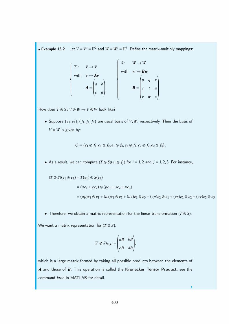
⌅ Example 13.2 Let V =V 0 = F2 and W =W 0 = F
3. Define the matrix-multiply mappings:
8>>>>>>>>><>>>>>>>>>:
T : V ! V
with vvv 7! AAAvvv
AAA =©≠≠´a b
c d
™Æƨ
8>>>>>>>>>>>><>>>>>>>>>>>>:
S : W ! W
with www 7! BBBwww
BBB =
©≠≠≠≠≠´
p q r
s t u
v w x
™ÆÆÆÆƨ
How does T ⌦ S : V ⌦ W ! V ⌦ W look like?
• Suppose {e1, e2}, { f1, f2, f3} are usual basis of V ,W , respectively. Then the basis of
V ⌦ W is given by:
C = {e1 ⌦ f1, e1 ⌦ f2, e1 ⌦ f3, e2 ⌦ f1, e2 ⌦ f2, e2 ⌦ f3}.
• As a result, we can compute (T ⌦ S)(ei ⌦ fj) for i = 1,2 and j = 1,2,3. For instance,
(T ⌦ S)(e1 ⌦ e1) = T(e1) ⌦ S(e1)
= (ae1 + ce2) ⌦ (pe1 + se2 + ve3)
= (ap)e1 ⌦ e1 + (as)e1 ⌦ e2 + (av)e1 ⌦ e3 + (cp)e2 ⌦ e1 + (cs)e2 ⌦ e2 + (cv)e2 ⌦ e3
• Therefore, we obtain a matrix representation for the linear transformation (T ⌦ S):
We want a matrix representation for (T ⌦ S):
(T ⌦ S)C,C =©≠≠´aB bB
cB dB
™Æƨ
,
which is a large matrix formed by taking all possible products between the elements of
AAA and those of BBB. This operation is called the Kronecker Tensor Product, see the
command kron in MATLAB for detail.
⌅
400
Proposition 13.6 More generally, given the linear operator T : V ! V and S : W ! W ,
let A = {v1, . . . ,vn},B = {w1, . . . ,wm} be a basis of V ,W respectively, with
(T)A,A = (ai j) (SB,B) = (bi j) := B
As a result, (T ⌦ S)C,C = A ⌦ B, where C = {v1 ⌦ w1, . . . ,vn ⌦ wm}, and A ⌦ B denotes the
Kronecker tensor product, defined as the matrix
©≠≠≠≠≠´
a1,1B · · · a1,nB... . . . ...
an,1B · · · an,nB
™ÆÆÆÆƨ
.
Proof. Following the similar procedure as in Example (13.2) and applying the relation
(T ⌦ S)(vi ⌦ wj) = T(vi) ⌦ S(wj)
=
n’
k=1
akivk
!⌦
m’`=1
b` jw`
!
=
n’k=1
m’`=1
(akib` j)vk ⌦ w`
⌅
Proposition 13.7 The operation T ⌦ S satisfies all the properties of tensor product. For
example,
(aT1 + bT2) ⌦ S = a(T1 ⌦ S) + b(T2 ⌦ S)
T ⌦ (cS1 + dS2) = c(T ⌦ S1) + d(T ⌦ S2)
Therefore, the usage of the notion “⌦” is justified for the definition of T ⌦ S.
Proof using matrix multiplication. For instance, consider the operation (T +T 0) ⌦ S, with
(T)A,A = (ai j), (T 0)A,A = (ci j), (S)B,B = B.
401
We compute its matrix representation directly:
((T +T 0) ⌦ S)C,C = (T +T 0)A,A ⌦ (S)B,B
= [(T)A,A + (T 0)A,A] ⌦ (S)B,B
= (T)A,A ⌦ (S)B,B + (T 0)A,A ⌦ (S)B,B
where the last equality is by the addictive rule for kronecker product for matrices.
Therefore,
((T +T 0) ⌦ S)C,C = (T ⌦ S)C,C + (T 0 ⌦ S)C,C =) (T +T 0) ⌦ S = T ⌦ S +T 0 ⌦ S
⌅
Proof using basis of T ⌦ S. Another way of the proof is by computing
((T +T 0) ⌦ S)(vi ⌦ wj),
where {vi ⌦ wj | 1 i n,1 j m} forms a basis of (T +T 0) ⌦ S:
((T +T 0) ⌦ S)(vi ⌦ wj) = (T +T 0)(vi) ⌦ S(wj)
= (T(vi) +T 0(vi)) ⌦ S(wj)
= T(vi) ⌦ S(wj) +T 0(vi) ⌦ S(wj)
= (T ⌦ S)(vi ⌦ wj) + (T 0 ⌦ S)(vi ⌦ wj)
Since ((T +T 0) ⌦ S)(vi ⌦ wj) coincides with (T ⌦ S +T 0 ⌦ S)(vi ⌦ wj) for all basis vectors
vi ⌦ wj 2 C, we imply
(T +T 0) ⌦ S = T ⌦ S +T 0 ⌦ S
⌅
Proposition 13.8 Let A,C be linear operators from V to V , and B, D be linear operators
from W to W , then
(A ⌦ B) � (C ⌦ D) = (AC) ⌦ (BD)
402
Proposition 13.9 Define linear operators A : V !V and B : W !W with dim(V),dim(W)<
1. Then
det(A ⌦ B) = (det(A))dim(W )(det(B))dim(V )
Corollary 13.3 There exists a linear transformation
� : Hom(V ,V) ⌦ Hom(W ,W)! Hom(V ⌦ W ,V ⌦ W)
with A ⌦ B 7! A ⌦ B
where the input of � is the tensor product of linear transformations, and the output is the
linear transformation.
Proof. Construct the mapping
� : Hom(V ,V) ⇥ Hom(W ,W)! Hom(V ⌦ W ,V ⌦ W)
with �(A, B) = A ⌦ B
The � is indeed bilinear: for instance,
�(pA+ qC, B) = (pA+ qC) ⌦ B
= p(A ⌦ B) + q(C ⌦ B)
= p�(A, B) + q�(C, B)
This corollary follows from the universal property of tensor product. ⌅
R If assuming that dim(V),dim(W) <1, we imply
dim(Input space of �) = dim(Hom(V ,V))dim(Hom(W ,W))
= [dim(V)dim(V)] · [dim(W)dim(W)] = [dim(V)dim(W)]2
= [dim(V ⌦ W)]2
= dim(Hom(V ⌦ W ,V ⌦ W))
= dim(Output space of �)
403

Therefore, is � is an isomorphism? If so, then every linear operator ↵ : V ⌦W !
V ⌦ W can be expressed as
↵ = A1 ⌦ B1 + · · · + Ak ⌦ Bk
where Ai : V ! V and Bj : W ! W .
404


Chapter 14
Week14
14.1. Monday for MAT3040
14.1.1. Multilinear Tensor ProductDefinition 14.1 [Tensor Product among More spaces] Let V1, . . . ,Vp be vector spaces
over F. Let S = {(v1, . . . ,vp) | vi 2 Vi} (We assume no relations among distinct elements in
S), and define X = span(S).
1. Then define the tensor product space V1 ⌦ · · · ⌦ Vp = X/y, where y is the vector
subspace of X spanned by vectors of the form
(v1, . . . ,vi + v0i , . . . ,vp) � (v1, . . . ,vi, . . . ,vp) � (v1, . . . ,v0i , . . . ,vp),
and
(v1, . . . ,↵vi, . . . ,vp) � ↵(v1, . . . ,vi, . . . ,vp)
where i = 1,2, . . . , p.
2. The tensor product for vectors is defined as
v1 ⌦ · · · ⌦ vp := {(v1, . . . ,vp) + y} 2 V1 ⌦ · · · ⌦ Vp
⌅
R Similar as in tensor product among two space,
417

1. We have
v1 ⌦ · · ·⌦ (↵vi + �v0i )⌦ · · ·⌦ vp =↵(v1 ⌦ · · ·⌦ vi ⌦ · · ·⌦ vp)+ �(v1 ⌦ · · ·⌦ v0i ⌦ · · ·⌦ vp)
2. A general vector in V1 ⌦ · · · ⌦ Vp is
n’i=1
(W (i)1 ⌦ · · · ⌦ W (i)
p ), where W (i)j 2 Vj , j = 1, . . . , p
3. Let Bi = {v(1)i , . . . ,v(dim(Vi ))i } be a basis of Vi, i = 1, . . . , p, then
B = {V (↵1)1 ⌦ · · · ⌦ V (↵p )
p | 1 ↵i dim(Vi)}
is a basis of V1 ⌦ · · · ⌦ Vp. As a result,
dim(V1 ⌦ · · · ⌦ Vp) = (dim(V1)) ⇥ · · · ⇥ (dim(Vp))
Theorem 14.1 — Universal Property of multi-linear tensor. Let Obj= {� : V1 ⇥ · · ·⇥Vp !
W | � is a p-linear map}, i.e.,
�(v1, . . . ,↵vi + �v0i , . . . ,vo) = ↵�(v1, . . . ,vi, . . . ,vp) + ��(v1, . . . ,v0i , . . . ,vp),
8vi,v0i 2 Vi, i = 1, . . . , p,8↵, � 2 F.
For instance, the multiplication of p matrices is a p-linear map.
Then the mapping in the Obj,
i : V1 ⇥Vp ! V1 ⌦ · · · ⌦ Vp
with (v1, . . . ,vp) 7! v1 ⌦ · · · ⌦ vp
satisfies the universal property. In other words, for any � : V1 ⇥ · · · ⇥Vp 2 Obj, there
418

exists the unqiue linear transformation
� : V1 ⌦ · · · ⌦ Vp ! W
such that the diagram below commutes:
In other words, � = � � i.
Corollary 14.1 Let Ti : Vi ! V 0i be a linear transformation, 1 i p. There is a unique
linear transformation
(T1 ⌦ · · · ⌦ Tp) : V1 ⌦ · · · ⌦ Vp ! V 01 ⌦ · · · ⌦ V 0
p
satisfying (T1 ⌦ · · · ⌦ Tp)(v1 ⌦ · · · ⌦ vp) = T1(v1) ⌦ · · · ⌦ Tp(vp)
Proof. Construct the mapping
� : V1 ⇥ · · · ⇥Vp ! V 01 ⌦ · · · ⌦ V 0
p
with (v1, . . . ,vp) 7! T1(v1) ⌦ · · · ⌦ Tp(vp)
which is indeed p-linear.
By the universal property, we induce the unique linear transformation
� : V1 ⌦ · · · ⌦ Vp ! V 01 ⌦ · · · ⌦ V 0
p
⌅
419

Notation. To make life easier, from now on, we only consider V1 = · · · = Vp = V . Then
for any linear transformation T : V ! W , we have
T ⌦p : V ⌦ · · · ⌦ V ! W ⌦ · · · ⌦ W
We use the short-hand notation V ⌦p to denote V ⌦ · · · ⌦ V| {z }p terms in total
Final Exam Ends Here.
14.1.2. Exterior PowerDefinition 14.2 A p-linear map � : V ⇥ · · · ⇥V ! W is called alternating if
�(v1, . . . ,vi, . . . ,vj , . . . ,vp) = 000W , provided that there exists some vi = vj for i , j.
Also, we say � is p-alternating ⌅
⌅ Example 14.1 1. The cross product mapping
� : R3 ⇥ R
3 ! R3
with (vvv,www) 7! vvv ⇥ www
is alternating:
• � is bilinear
• �(vvv,vvv) = vvv ⇥ vvv = 000.
2. The determinant mapping
� : Fn ⇥ · · · ⇥ F
n| {z }n terms in total
! F
with (vvv1, . . . ,vvvn) 7! det([vvv1,vvv2, · · · ,vvvn])
is alternating:
420

• � is n-linear by MAT2040 knowledge
• � is alternating by MAT2040 knowledge
⌅
Theorem 14.2 — Universal Property for exterior power. Let Obj := {� : V ⇥ · · ·V| {z }p terms
!W |
� is p-alternating map}. Then there exists {⇤ : V ⇥ · · · ⇥V ! E} 2 Obj satisfying the
following:
• For all � : V ⇥ · · · ⇥ V ! W 2 Obj, there exists unique linear transformation
� : E ! W satisfying
In other words, � = � �⇤.
421

Chapter 15
Week15
15.1. Monday for MAT3040
15.1.1. More on Exterior PowerReviewing. Let Obj := {� : V ⇥ · · · ⇥V ! W | � is alternating}, then there exists
{⇤ : V ⇥ · · · ⇥V ! E} 2 Obj
such that
� = � �⇤, where � : E ! W is the unique linear transformation
Here we give one way for constructing E :
E = V ⌦p/U,
where U is spanned by vectors of the form
v1 ⌦ · · · ⌦ vp 2 V ⌦p, vi = vj where for some i , j.
For instance, v ⌦ v ⌦ · · · ⌦ vp 2 U.
431
Definition 15.1 [Wedge Product] Define the wedge product space
^pV := V ⌦p/U = E ,
with the wedge product among vectors
v1 ^ · · · ^ vp = v1 ⌦ · · · ⌦ vp +U 2 ^pV
⌅
As a result, the mapping
^ : V ⇥ · · · ⇥V ! E := ^pV
(v1, . . . ,vp) 7! v1 ^ · · · ^ vp
will satisfy the universal property of exterior power.
Proposition 15.1 1. We have the p-linearity for ^pV , i.e.,
v1 ^ · · · ^ (avi + bv0i )^ · · · ^ vp = a(v1 ^ · · · ^ vi ^ · · · ^ vp) + b(v1 ^ · · · ^ v0i ^ · · · ^ vp)
for i = 1, . . . , p.
2. The wedge product is alternating:
v1 ^ · · · ^ v ^ · · · ^ v ^ · · · ^ vp := v1 ⌦ · · · ⌦ v ⌦ · · · ⌦ v ⌦ · · · ⌦ vp +U
= 0 +U
= 0^pV
3. The wedge product reverses sign reversal property:
v1 ^ · · · ^ v ^ · · · ^ w ^ · · · ^ vp = �v1 ^ · · · ^ w ^ · · · ^ v ^ · · · ^ vp
Reason: (v + w)^ (v + w) = 0, which implies v ^ w + w ^ v = 0.
432

Proposition 15.2 1. If dim(V) = n, and 0 p n, then
dim(^pV) =✓np
◆
2. For all linear operators T : V ! V , there is an unique linear operator from ^pV to
^pV :T^p : ^pV !^pV
with v1 ^ · · · ^ vp 7! T(v1)^ · · · ^T(vp)
Proof. 1. Let {v1, . . . ,vn} be basis of V , then {vi1 ⌦ · · · ⌦ vip | 1 ik n} forms basis
of V ⌦p. Note that {vi1 ^ · · · ^ vip | 1 ik n} spans ^pV , since ⇡V : V ! V/U is
surjective. We claim that
B = {vi1 ^ · · · ^ vip | 1 i1 < i2 < · · · < ip n}
is a basis of ^pV
• B spans ^pV : we can use (3) in proposition (15.1) to “rearrange” the indices
j1, . . . , jp into ascending order, and span(B) = span{vi1 ^ · · · ^ vip | 1 ik n}.
• We omit the proof that B is linear independent due to time limit.
The numbre of vectors in B is equal to�np
�.
⌅
15.1.2. Determinant
Previous Approach for defining determinant. We define the determinant for
AAA = Mn⇥n(F) directly. From such complicated definition, we come up with det(AAABBB) =
det(AAA)det(BBB), which implies that the similar matrices share with the same determinant,
then we define the determinant for any linear operator T : V ! V as
det(T) = det((T)B,B), for some basis B of T
433

New Approach. We will define det(T) for linear operators without fixing a basis,
and then we will imply det(T � S) = det(T)det(S) easily. Then det(AAA) for AAA 2 Mn⇥n(F)
belongs to our special case.
Definition 15.2 [Determinant for Linear Operators]
1. Suppose that dim(V) = n, then
dim(^nV) =✓nn
◆= 1
More precisely, for any basis {v1, . . . ,vn} of V , we have ^n(V) = span{v1 ^ · · · ^ vn}.
2. Note tht T^n : ^nV ! ^nV is a linear operator on ^nV � F. Therefore, for all
⌧ 2 ^nV , there exists ↵T 2 F such that
T^n (⌧) = ↵T ⌧
3. Now we define
det(T) = ↵T
This definition of determinant does not depend on any choice of basis of V .
⌅
⌅ Example 15.1 1. Suppose that T = I : V ! V be identity. Take a basis {v1, . . . ,vn}
of V , then
T^n (v1 ^ · · · ^ vn) = T(v1)^ · · · ^T(vn)
Or equivalently,
det(T) · (v1 ^ · · · ^ vn) = v1 ^ · · · ^ vn
Therefore, det(T) = 1.
2. Suppose that T : V ! V is diagonalizable with {w1, . . . ,wn} forming eigen-basis of
T .
434
As a result,
T^n (w1 ^ · · · ^ wn) = T(w1)^T(w2) · · · ^T(wn),
which implies
det(T)(w1 ^ · · · ^ wn) = (�1w1)^ · · · ^ (�nwn),
which implies
det(T)w1 ^ · · · ^ wn = (�1 · · ·�n)w1 ^ · · · ^ wn,
i.e., det(T) = �1 · · ·�n.
⌅
Proposition 15.3 Let T , S : V ! V be linear transformations, then
(T � S)^p : ^pV !^pV
with T^p , S^p : ^pV !^pV
satisfies
(T � S)^p= (T^p ) � (S^p )
Proof. Pick any basis {vi1 ^ · · · ^ vip | 1 i1 < · · · < ip n} of ^pV . Then
(T � S)^p (vi1 ^ · · · ^ vip ) = (T � S)(vi1)^ · · · ^ (T � S)(vip )
On the other hand,
(T^p ) � (S^p )(vi1 ^ · · · ^ vip ) = (T^p )(S(vi1)^ · · · ^ S(vip ))
= (T � S)(vi1)^ · · · (T � S)(vip )
⌅
Corollary 15.1
det(T � S) = det(T)det(S)
435
Proof. Pick any basis {v1 ^ · · · ^ vn} of ^nv, then
det(T � S)v1 ^ · · · ^ vn = (T � S)^nv1 ^ · · · ^ vn
= (T^n ) � ((S^n )v1 ^ · · · ^ vn)
= (T^n )(det(S)v1 ^ · · · ^ vn)
= det(S)T^n (v1 ^ · · · ^ vn)
= det(S)det(T)v1 ^ · · · ^ vn
Therefore, det(T � S) = det(T)det(S).
⌅
Theorem 15.1 Let V = Fn, and
T : V ! V
with T(vvv) = AAAvvv, AAA 2 Mn⇥n(F)
Then det(T) = det(AAA)
Proof. Take {e1, . . . , en} as the usual basis of V ⌘ Fn, then
det(T)e1 ^ · · · ^ en = T(e1)^ · · ·T(en)
= a1 ^ · · · ^ an
where ai denotes the i-th column of AAA.
As we have studied before [c.f. p141 in MAT2040 Notebook], the previous definition
of determinant is based on three basic properties. It suffices to show these three basis
properties:
1. The determinant of the n by n identity matrix is 1: See part (1) in Example (15.1)
2. The determianant changes sign when two columns (w.l.o.g., “rows” are relaced
with “columns”) are exchanged: due to the sign reversal property for wedge
product
436
3. The determinant is a linear function of each column separately, i.e.,
a1 ^ · · · ^ (tai)^ · · · ^ an = t(a1 ^ · · · ^ ai ^ · · · ^ an)
Once we verify these three properties, we conclude that the explicit formula for det(AAA)
is a special case for our new definition. ⌅
Or we can come into the previous definition for determinant directly. For instance,
consider the mapping
T : R2 ! R2
with T©≠≠´
x
y
™Æƨ=©≠≠´a b
c d
™Æƨ©≠≠´
x
y
™Æƨ
Then we imply
det(T)(e1 ^ e2) =©≠≠´a
c
™Æƨ^©≠≠´
b
d
™Æƨ
= (ae1)^ (be1) + (ae1)^ (de2) + (ce2)^ (de1) + (ce2)^ (de2)
= (ad)e1 ^ e2 + (bc)e2 ^ e1
= (ad � bc)e1 ^ e2
Therefore, we imply det(T) = ad � bc.
437