
Advanced kinematics and dynamics of the upper limb … · En résumé, cette thèse a permis de...
163
Advanced kinematics and dynamics of the upper limb for clinical evaluation Alexandre Naaim To cite this version: Alexandre Naaim. Advanced kinematics and dynamics of the upper limb for clinical evaluation. Biomechanics [physics.med-ph]. Universit´ e de Lyon, 2016. English. <tel-01321375v1> HAL Id: tel-01321375 https://hal.archives-ouvertes.fr/tel-01321375v1 Submitted on 25 May 2016 (v1), last revised 6 Jan 2016 (v2) HAL is a multi-disciplinary open access archive for the deposit and dissemination of sci- entific research documents, whether they are pub- lished or not. The documents may come from teaching and research institutions in France or abroad, or from public or private research centers. L’archive ouverte pluridisciplinaire HAL, est destin´ ee au d´ epˆ ot et ` a la diffusion de documents scientifiques de niveau recherche, publi´ es ou non, ´ emanant des ´ etablissements d’enseignement et de recherche fran¸cais ou ´ etrangers, des laboratoires publics ou priv´ es.
Transcript of Advanced kinematics and dynamics of the upper limb … · En résumé, cette thèse a permis de...

Advanced kinematics and dynamics of the upper limb
for clinical evaluation
Alexandre Naaim
To cite this version:
Alexandre Naaim. Advanced kinematics and dynamics of the upper limb for clinical evaluation.Biomechanics [physics.med-ph]. Universite de Lyon, 2016. English. <tel-01321375v1>
HAL Id: tel-01321375
https://hal.archives-ouvertes.fr/tel-01321375v1
Submitted on 25 May 2016 (v1), last revised 6 Jan 2016 (v2)
HAL is a multi-disciplinary open accessarchive for the deposit and dissemination of sci-entific research documents, whether they are pub-lished or not. The documents may come fromteaching and research institutions in France orabroad, or from public or private research centers.
L’archive ouverte pluridisciplinaire HAL, estdestinee au depot et a la diffusion de documentsscientifiques de niveau recherche, publies ou non,emanant des etablissements d’enseignement et derecherche francais ou etrangers, des laboratoirespublics ou prives.

i
N° d’ordre : Année 2015
THESE DE L‘UNIVERSITE DE LYON
Délivrée par
L’UNIVERSITE CLAUDE BERNARD LYON 1
ECOLE DOCTORALE :
MEGA spécialité Biomécanique
DIPLOME DE DOCTORAT
(arrêté du 7 août 2006)
Soutenue publiquement le 15 janvier 2016 par
Alexandre NAAIM
Modélisation cinématique et dynamique avancée du membre supérieur pour l’analyse clinique
Advanced kinematics and dynamics of the upper limb for clinical evaluation
Directeur de thèse: Laurence CHEZE
Co-Directeur de thèse: Thierry HAUMONT
Devant le jury composé de
Mickael BEGON Professeur, S2M, Montreal (CA) Rapporteur Frans C.T VAN DER HELM Professeur, Delft university of Technology, Delft (NL) Rapporteur Laurence CHEZE Professeur des Universités, UCBL, Lyon (FR) Examinateur Thierry HAUMONT PU-PH, CHU de Caen (FR) Examinateur Fabien LEBOEUF Chercheur (PhD), University of Salford, Salford (UK) Examinateur Florent MOISSENET Ingénieur (PhD), CNRFR-Rehazenter, Luxembourg (LU) Examinateur Sylvain BROCHARD MCU-PH, CHU de Brest (FR) Examinateur

i
UNIVERSITE CLAUDE BERNARD - LYON 1
Président de l’Université
Vice-président du Conseil d’Administration
Vice-président du Conseil des Etudes et de la Vie Universitaire
Vice-président du Conseil Scientifique
Directeur Général des Services
M. François-Noël GILLY
M. le Professeur Hamda BEN HADID
M. le Professeur Philippe LALLE
M. le Professeur Germain GILLET
M. Alain HELLEU
COMPOSANTES SANTE
Faculté de Médecine Lyon Est – Claude Bernard
Faculté de Médecine et de Maïeutique Lyon Sud – Charles Mérieux
Faculté d’Odontologie
Institut des Sciences Pharmaceutiques et Biologiques
Institut des Sciences et Techniques de la Réadaptation
Département de formation et Centre de Recherche en Biologie Humaine
Directeur : M. le Professeur J. ETIENNE
Directeur : Mme la Professeure C. BURILLON
Directeur : M. le Professeur D. BOURGEOIS
Directeur : Mme la Professeure C. VINCIGUERRA
Directeur : M. le Professeur Y. MATILLON
Directeur : Mme. la Professeure A-M. SCHOTT
COMPOSANTES ET DEPARTEMENTS DE SCIENCES ET TECHNOLOGIE
Faculté des Sciences et Technologies
Département Biologie
Département Chimie Biochimie
Département GEP
Département Informatique
Département Mathématiques
Département Mécanique
Département Physique
UFR Sciences et Techniques des Activités Physiques et Sportives
Observatoire des Sciences de l’Univers de Lyon
Polytech Lyon
Ecole Supérieure de Chimie Physique Electronique
Institut Universitaire de Technologie de Lyon 1
Ecole Supérieure du Professorat et de l’Education
Institut de Science Financière et d'Assurances
Directeur : M. F. DE MARCHI
Directeur : M. le Professeur F. FLEURY
Directeur : Mme Caroline FELIX
Directeur : M. Hassan HAMMOURI
Directeur : M. le Professeur S. AKKOUCHE
Directeur : M. le Professeur Georges TOMANOV
Directeur : M. le Professeur H. BEN HADID
Directeur : M. Jean-Claude PLENET
Directeur : M. Y.VANPOULLE
Directeur : M. B. GUIDERDONI
Directeur : M. P. FOURNIER
Directeur : M. G. PIGNAULT
Directeur : M. le Professeur C. VITON
Directeur : M. le Professeur A. MOUGNIOTTE
Directeur : M. N. LEBOISNE

ii
Abstract
Keywords: Soft tissue artefact, multibody optimisation, human movement analysis, stereophotogrammetry, modelling, upper limb,
Soft Tissue Artefact (STA) is one of the most important limitations when measuring upper limb kinematics through marker-based motion capture techniques, especially for the scapula. Multi Body Optimisation (MBO) has already been proposed to correct STA when measuring lower limb kinematics and can be easily adapted for upper limb. For this purpose, the joint kinematic constraints should be as anatomical as possible.
The aim of this thesis was thus to define and validate an anatomical upper limb kinematic model that could be used both to correct STA through the use of MBO and for future musculoskeletal models developments. For this purpose, a model integrating closed loop models of the forearm and of the scapula belt have been developed, including a new anatomical-based model of the scapulothoracic joint. This model constrained the scapula plane to be tangent to an ellipsoid modelling the thorax.
All these models were confronted to typical models extracted from the literature through cadaveric and in vivo intracortical pins studies. All models generated similar error when evaluating their ability to mimic the bones kinematics and to correct STA. However, the new forearm and scapulothoracic models were more interesting when considering further musculoskeletal developments: The forearm model allows considering both the ulna and the radius and the scapulothoracic model better represents the constraint existing between the thorax and the scapula.
This thesis allowed developing a complete anatomical upper limb kinematic chain. Although the STA correction obtained was not as good as expected, the use of this approach for a future musculoskeletal models has been validated.

iii
Résumé
Mots-clés: Artefact des tissus mous, optimisation multi-segmentaire, analyse du mouvement, stéréophotogrammétrie, modélisation, membre supérieur
Les Artefacts de Tissus Mous (ATM) sont actuellement une des limitations principales pour la mesure du mouvement du membre supérieur avec les techniques actuelles d'analyse du mouvement. L’optimisation multi-segmentaire (OMS) a déjà prouvé son efficacité pour la mesure du mouvement du membre inférieur. Afin d’avoir la meilleure correction possible, il est nécessaire d’utiliser des modèles d’articulation proches de l’anatomie. L’objectif de cette thèse a donc été de développer et de valider un modèle du membre supérieur qui pourrait être utilisé pour la correction des ATM par OMS.
De nouveaux modèles en boucle fermée de l’avant-bras et de la ceinture scapulaire ont ainsi été développés accompagnés d’un nouveau modèle de l’articulation scapulo-thoracique imposant à la scapula d’être tangente à un ellipsoïde modélisant le thorax. Ces nouveaux modèles ont été confrontés aux modèles courants de la littérature à travers une étude avec vis intra-corticales sur cadavre et in vivo sur sujets asymptomatiques.
Des niveaux d’erreur similaires ont été observés pour tous les modèles quant à leur capacité de corriger les ATM et d’imiter la cinématique osseuse. Les nouveaux modèles semblent cependant beaucoup plus intéressants dans une perspective de développement d’un modèle musculo-squelettique. En effet, le modèle d’avant-bras autorise à la fois d’avoir le mouvement du radius et de l’ulna tandis que le modèle scapulo-thoracique représente mieux la contrainte existant entre le thorax et la scapula.
En résumé, cette thèse a permis de développer un modèle complet proche de l’anatomie du membre supérieur permettant de corriger les ATM en utilisant une OMS. Bien que la correction des ATM obtenue n’est pas aussi satisfaisante qu’espérée, l’utilisation de cette approche pour le développement de futurs modèles musculo-squelettique a été validée.

iv
Remerciements
Je souhaite tout d’abord exprimer ma gratitude au Fonds National de la Recherche Luxembourgeois pour avoir financé l’ensemble de cette thèse. Je voulais aussi remercier Frans C.T Van der Helm et Mickael Begon d’avoir accepté d’évaluer cette thèse, ainsi que Fabien Lebœuf et Sylvain Brochard de faire partie du jury.
A l’issue de ce travail, je suis convaincu que même si la thèse est parfois un travail solitaire elle ne peut pas être réalisée sans le soutien d’un grand nombre de personnes. J’ai eu l’occasion de pouvoir réaliser ce doctorat entre différents laboratoires, de Luxembourg à Lyon, en passant par Caen ou Montréal. J’ai ainsi pu partager cette aventure avec de nombreuses personnes qui sont venues enrichir ce travail de leurs expériences et de leurs connaissances. Sans eux, cette thèse ne serait sûrement pas ce qu’elle est aujourd’hui et je tenais à les en remercier.
Je voulais donc tout d’abord remercier le Centre National de Rééducation Fonctionnelle et de Réadaptation du Luxembourg (CNRFR–Rehazenter) pour m’avoir accueilli au sein de sa structure pour réaliser l’ensemble de ce travail. Je pense tout particulièrement à l’équipe du laboratoire d’analyse du mouvement et de la posture qui m’a accompagné au jour le jour (Dr.Paul Filipetti, Dr.Frederic Chantraine, Dr.Elisabeth Kolanowski, Angelique Remacle et Celine Schreiber). Un remerciement un peu plus spécifique à Florent Moissenet qui m’a encadré et a toujours réussi à canaliser (et supporter) mon trop plein d’énergie. Son implication dans le laboratoire et sa motivation constante ont été dans les moteurs principaux de l’ensemble de cette thèse. Merci de m’avoir toujours impliqué dans les discussions relatives à la recherche clinique ou aux développements du laboratoire. J’ai pu grâce à toi me construire une solide connaissance du fonctionnement d’un laboratoire d’analyse du mouvement en clinique. Si je ne devais avoir qu’un regret dans cette thèse c’est de ne pas avoir pu travailler de manière plus importante avec toi.
Mes remerciements vont également à ma directrice de thèse Laurence Chèze ainsi qu’à Raphaël Dumas pour m’avoir accueilli et encadré au sein du Laboratoire de Biomécanique et Mécanique des Chocs et de m’avoir suivi tout au long de cette thèse. La semaine mensuelle que j’ai pu passer à Lyon a sensiblement participé au bon déroulement de ce travail. Les discussions que nous avons pu avoir m’ont permis d’avancer tant scientifiquement que personnellement. Un grand merci à vous pour vos conseils, votre dynamisme, et votre disponibilité.
Les expérimentations réalisées au cours de cette thèse n’auraient pas été possibles sans la participation de mon co-directeur de thèse, le Dr. Thierry Haumont, que je tiens aussi à remercier. Merci de m’avoir ouvert les portes du laboratoire d’anatomie du CHU de Caen et de m’avoir fait confiance et aidé pour l’ensemble de ces travaux. Un remerciement aussi au Dr. Jean-Pierre Pelage et son équipe pour avoir exceptionnellement accepté d’ouvrir leur service d’imagerie en dehors des horaires d’ouverture pour que nous puissions réaliser nos différentes acquisitions.

v
Finalement, merci à Mickael Begon pour m’avoir accueilli pendant mon stage de trois mois dans son laboratoire (S2M) à Montréal. J’ai ainsi pu confronter mes différents modèles à la réalité expérimentale mais aussi à la rigueur du froid québécois. Merci à toute son équipe (Diane, Benjamin, Pat, Ariane, Colombes, Fabien et tous les autres) qui a su m’accueillir très chaleureusement contrairement à la météo.
Je remercie aussi tous les autres doctorants du LBMC avec qui j’ai eu l’occasion de travailler au cours de cette thèse (Xavier, Angèle, Cindy, Julien, Stéphane, Brice, Pascal, Sylvie, Vincent, Romain). Merci pour toutes les pauses café (‘La machine à café est l’endroit où la recherche avance’), les conseils et la bonne ambiance qui pouvait régner dans la salle doctorant grâce à vous.
Je tenais aussi à remercier mes colocs luxembourgeois (Marion, Ivan, Nicolas, Mélanie, les Rémi et les Clément) pour tous les bons moments de vie au RO85. La vie au Luxembourg aurait été beaucoup plus ennuyeuse sans vous.
D’une manière générale, je voulais remercier chaleureusement tous mes amis (Nico, Jérémie, Thibaut, Elodie, Sandra, Hugo, Alain, André, Justine et tous les autres) pour avoir été là dans tous les moments depuis toutes ces années. Je voudrais remercier plus particulièrement ceux qui ont toujours eu la porte ouverte pour m’accueillir lors de mes semaines lyonnaises. Merci à Calwin, Daniel, Bastien, Blandine, Maxime, Baptiste et Magalie qui ont su m’offrir l’hospitalité en toute occasion et me rappeler qu’on peut toujours compter sur ses amis.
Pour finir, je voudrais adresser toute mon affection à l’ensemble de ma famille. Merci pour tout l’amour et le soutien sans faille qu’ils m’ont donné tout au long de ma vie et de mes études, des plus petites classes de maternelles jusqu’à la fin, aujourd’hui, de mon doctorat. Merci pour toutes ces innombrables choses que vous m’avez apportées, petites et grandes qui font ce que je suis aujourd’hui.
Merci à tous pour ces trois années qui sans vous n’aurez pas été les mêmes !

vi
Table of contents
Abstract ............................................................... ii
Résumé ................................................................ iii
Remerciements .....................................................iv
General introduction ............................................. 1
1. Preamble .............................................................................. 1
1.1. Motion Capture.................................................................................................. 2
1.2. Associated limitations ........................................................................................ 3
2. Aim of the thesis .................................................................. 4
3. Document organisation ......................................................... 5
Correction methods and models available ............. 7
1. Correction methods for STA-related errors .......................... 8
1.1. Regression formulae ........................................................................................... 8
1.2. Double calibration .............................................................................................. 9
1.3. Optimisation method ........................................................................................ 10
2. Existing models................................................................... 12
2.1. Shoulder ............................................................................................................ 13
2.1.1. Glenohumeral ........................................................................................................ 13
2.1.2. Shoulder girdle ....................................................................................................... 14
2.1.2.1. Equivalent mechanism: first approximation for modelling shoulder girdle...... 15
2.1.2.2. Anatomical representation: Open loop vs Closed loop .................................... 16
Open loop model: Considering the different bony structures of the shoulder girdle 16
Closed loop model: Integration of the scapulothoracic joint .................................... 17
2.2. Forearm model: integration of a real pronosupination ..................................... 18
2.2.1. Simple model: Integration of the ulna and radius ................................................. 20
2.2.2. Integration of a more realistic joint kinematic model: Lemay, Pennestri and Weinberg models ............................................................................................................. 20

Table of contents
vii
2.2.3. Integration of supplementary degrees of freedom. ................................................. 23
3. Geometric parameters ........................................................ 24
3.1. Prediction methods ........................................................................................... 24
3.2. Regression and scaling methods ........................................................................ 25
3.3. Functional methods .......................................................................................... 26
3.4. Imaging techniques ........................................................................................... 26
4. Validation procedures ......................................................... 28
4.1. Imaging techniques ........................................................................................... 28
4.2. Palpation methods ............................................................................................ 29
4.3. Intracortical pins ............................................................................................... 30
5. Thesis choices: .................................................................... 31
Theoretical background ....................................... 32
1. Natural coordinates and non-orthogonal coordinate system 32
2. Multibody system with natural coordinates ........................ 34
3. Upper limb model ............................................................... 35
3.1. Kinematics calculation ...................................................................................... 38
3.2. Virtual marker and vector definition ................................................................ 39
4. Multibody optimisation ...................................................... 40
4.1. Motor constraints .............................................................................................. 40
4.2. Rigid body constraints ...................................................................................... 41
4.3. Kinematic constraints ....................................................................................... 42
4.3.1. Scapulothoracic joint ............................................................................................. 42
4.3.1.1. Model tangent to an ellipsoid .......................................................................... 42
4.3.1.2. Contact point model ....................................................................................... 45
4.3.2. Clavicle .................................................................................................................. 47
4.3.3. Glenohumeral joint ................................................................................................ 48
4.3.3.1. Case 1: Spherical joint .................................................................................... 48
4.3.3.2. Case 2: Constant length .................................................................................. 49
4.3.4. Forearm ................................................................................................................. 49

Table of contents
viii
4.3.4.1. Humeroradial joint .......................................................................................... 49
4.3.4.2. Humeroulnar joint ........................................................................................... 50
4.3.4.3. Distal radioulnar joint ..................................................................................... 51
4.3.5. Wrist ..................................................................................................................... 51
4.4. Final formulation .............................................................................................. 52
Cadaveric study .................................................. 53
1. Experimental protocol ........................................................ 54
1.1. Cadaver preparation ......................................................................................... 54
1.2. Motion capture protocol ................................................................................... 57
1.3. CT-scan ............................................................................................................. 58
1.4. Model generation .............................................................................................. 59
1.5. Models comparison ............................................................................................ 61
1.6. Contact point .................................................................................................... 62
1.6.1. Definition ............................................................................................................... 62
1.6.2. Equation ................................................................................................................ 64
2. Results ................................................................................ 65
2.1. Scapulothoracic joint ........................................................................................ 65
2.1.1. Kinematics ............................................................................................................. 65
2.1.1.1. Upward-downward rotation ............................................................................ 69
2.1.1.2. Protraction-retraction ..................................................................................... 69
2.1.1.3. Anterior-posterior tilt ...................................................................................... 69
2.1.2. Contact point ........................................................................................................ 70
2.2. Forearm ............................................................................................................. 72
3. Discussion ........................................................................... 73
3.1. Scapulothoracic model ...................................................................................... 73
3.1.1. Kinematics ............................................................................................................. 73
3.1.2. Contact point ........................................................................................................ 74
3.1.3. Ellipsoid definition ................................................................................................. 75
3.2. Forearm model .................................................................................................. 77
4. Limits ................................................................................. 77

Table of contents
ix
5. Conclusion .......................................................................... 78
In vivo intracortical experimentation .................. 79
1. Validation data ................................................................... 81
1.1. Intracortical pins ............................................................................................... 81
1.2. Comparison method .......................................................................................... 83
2. Study 1: Ability of the different MBO models to mimic the bones kinematics ..................................................................... 84
2.1. Methods ............................................................................................................ 84
2.2. Results .............................................................................................................. 85
2.2.1. Anterior-posterior tilt ............................................................................................ 87
2.2.2. Protraction-retraction ............................................................................................ 87
2.2.3. Upward-downward rotation ................................................................................... 88
2.3. Discussion ......................................................................................................... 88
3. Study 2: Ability of the different MBO models to correct Soft Tissue Artefact ....................................................................... 88
3.1. Method .............................................................................................................. 88
3.2. Results: using ISB motor constraints ................................................................ 89
3.2.1. Upward-downward rotation ................................................................................... 91
3.2.2. Protraction-retraction ............................................................................................ 91
3.2.3. Anterior-posterior tilt ............................................................................................ 92
3.3. Results: using Jackson et al. motor constraints ................................................ 92
3.3.1. Upward-downward rotation ................................................................................... 92
3.3.2. Protraction-retraction ............................................................................................ 92
3.3.3. Anterior-posterior tilt ............................................................................................ 93
3.4. Discussion ......................................................................................................... 95
4. Study 3: Simpler STA correction method ........................... 96
4.1. The neglected-Degree of Freedom method........................................................ 97
4.1.1. Equation ................................................................................................................ 97
4.1.2. Experimentation: definition of different marker sets ............................................. 98
4.2. Results .............................................................................................................. 99

Table of contents
x
4.2.1. Anterior-posterior tilt ............................................................................................ 99
4.2.2. Upward-downward rotation ................................................................................... 99
4.2.3. Protraction-retraction .......................................................................................... 100
4.3. Discussion ....................................................................................................... 102
5. Limits ............................................................................... 103
6. Conclusion ........................................................................ 104
General conclusion ............................................ 106
1. Thesis outcomes ................................................................ 106
1.1. MultiBody Optimisation as a tool for correcting Soft Tissue Artefact ........... 106
1.2. Kinematic chain model development .............................................................. 106
1.3. Models validation: Intracortical pins .............................................................. 107
1.4. Conclusion ....................................................................................................... 107
2. Perspectives ...................................................................... 108
Bibliography ...................................................... 113
List of figures .................................................... 122
List of tables ..................................................... 127
Appendix ........................................................... 128

1
General introduction
1. Preamble The main upper limb functionality is to set the end-effector (i.e., the hand) position and orientation in space, with or without load. In order to achieve this task, a compromise between mobility and stability, strength and loading has to constantly be found. Since the upper limb is often required for repetitive tasks, these constraints can become traumatic and induce osteo-articular or musculo-tendinous disorders (Anglin and Wyss, 2000). The upper limb is also highly impacted by neurological pathologies such as cerebral palsy, hemiplegia, paraplegia or tetraplegia. In that case, the movements of the patient is faced with different motor control impairments (e.g., muscle lack of selectivity, weakness, spasticity). It results in important deficiencies in performance of daily activities and impacts thus directly the quality of life and the independency of the patient. In order to choose an adapted treatment for each patient, an evaluation of the different impairments of their upper limbs is essential. The assessment of these patients is mainly based on a clinical evaluation (e.g., muscle strength, spasticity, range of motion). Sometimes, this evaluation is completed by clinical scales based on functional movements (e.g., Melbourne Assessment of Unilateral Upper Limb Function (Bourke-Taylor, 2003), Quality of Upper Extremity Skill Test (DeMatteo et al., 1992)). However, all these evaluations tend to stay more qualitative than quantitative and can be subjective as they are based on the observation of an assessor. In addition, some tasks might not be sensitive enough to detect changes that would be relevant clinically (Sätilä et al., 2006). Consequently, there is a lack of quantitative analysis in the evaluation of the upper limb in a clinical context.
Some quantitative analysis can be found through the literature and focus commonly on two elements: spatiotemporal characteristics and joint kinematics (Jaspers et al., 2009). The spatiotemporal characteristic are generally associated to the time taken by the subject to perform a specific functional task corresponding to daily activities (e.g., reach and grasp, hand to mouth, hand to back…). This allows having a global quantitative evaluation of the upper limb. However, in order to be able to identify the different compensatory movements or patterns that can exist, and then allow for more precise diagnosis, there is a need to focus on each joint separately. For this purpose, analysing the different joint kinematics and dynamics is useful. It can allow relating the different movement impairment characteristics to the underlying pathology and define different classifications based on these findings. However, the kinematic and dynamic explorations of the whole upper limb during a movement remains challenging. The diagnosis and treatment prescription are thus limited. The main difficulty is located at the shoulder, composed of five high mobility joints and a complex polyarticular muscles layout. A better understanding of the shoulder complex functioning during a movement could allow significant improvements in terms of diagnosis and treatment.

General introduction
2
Motion analysis is a solution that can be used to reach this goal. Its principle is to determine the position and orientation of different body segments in space. This allows obtaining derived information such as the kinematics of each joint by the knowledge of the position and orientation of the anatomical coordinates systems embedded in the body segments. This methodology is already widely used to study the lower limb kinematics when exploring gait (Cappozzo et al., 2005; McGinley et al., 2009; Woltring, 1994). Gait is an efficient movement allowing the energy loss minimisation during the transport of the human body. It is an automatic and repeatable movement. Consequently, the definition and the comparison with normative data is relatively easy and adaptable in a clinical context. Unlikely, due to the high range of motion of the different joints constituting the upper limb, several strategies can arise for a similar task between subjects (Rau et al., 2000). It results that the definition of normative data, classification or the comparison between subjects is much more challenging than for lower limb in a clinical context. Beyond these problems linked to the complexity of the upper limb, the evaluation of the upper limb remains difficult due to technical limitations described below.
1.1. Motion Capture
One of the most common techniques in motion analysis is stereophotogrammetry. Stereophotogrammetry allows determining the spatial position of an object based on multiple cameras recordings. The main technology used is based on optoelectronic cameras which allow reconstructing the 3D position of passive cutaneous reflective markers bouncing back an infrared light emitted by the cameras. Using this technology, the precision for a marker position can be below 1 mm (Chiari et al., 2005).
In order to use stereophotogrammetry, the position and the orientation of each camera must be known. A calibration procedure is thus needed. This procedure must be done carefully as if it is done poorly, errors on the markers position can arise. Basically, the calibration results in the definition of the laboratory coordinate system (i.e., the inertial coordinate system or ICS) and the position and orientation of each camera in this coordinate system. Once this calibration has been performed, markers glued on the skin can be used to define the Segment Coordinate System (SCS) of the associated body segments. Indeed, these body segments are generally considered as non-deformable as the global interest is their position in space.
Different approaches have been proposed to determine SCSs. On one hand, SCSs can be geometrically defined directly through a set of cutaneous markers positioned on palpated anatomical landmarks. These landmarks are generally associated to bony prominences that can be palpated in a repeatable manner (Van Sint Jan, 2007). The axes, defined using these markers, must then approximate as precisely as possible the different anatomical planes (i.e., frontal, transverse and sagittal planes) of the segments. On the other hand, SCSs can be obtained through a Calibrated Anatomical System Technique (CAST) (Cappozzo et al., 2005). Using CAST, a cluster of markers is positioned on each body segment to define a local technical coordinate

General introduction
3
system. These clusters can be placed directly on the skin, on an elastic band or on a rigid plate attached to the body segment. In order to determine the SCSs, each anatomical landmark position is then defined during a static posture data collect and assumed fixed in this technical coordinate system. Thus, it is possible to compute the position of the SCS during the complete motion. The main interest of the CAST method is the possibility to choose the position of the cluster considering other constraints (e.g., the markers forming the cluster can be for example positioned in order to avoid any marker visual loss during acquisition or to minimise their movement with respect to the underlying bones). Finally, once each SCS has been defined, joint kinematics can be computed through Euler angles definition (Wu et al., 2002).
1.2. Associated limitations
Even with a technology able to determine the position of reflective markers with a precision under a millimeter, some limits exist when using stereophotogrammetry. A first limit is the palpation technique used for determining the different anatomical landmarks. Indeed, their positioning impacts directly on the SCS and thus kinematic calculations. Consequently, if the intra-/inter-session and/or operator repeatability is low due to a poor palpation technique, differences can arise in angles patterns without any change of the subject kinematics. This can be illustrated by a phenomenon called cross talk phenomenon. If the main rotation axis (e.g., knee flexion-extension axis) is poorly defined, the associated rotation will be reverberated in another rotation axis (e.g., knee abduction-adduction) (Della Croce et al., 2005; Piazza and Cavanagh, 2000).
Another limit is called Soft Tissue Artefact (STA). STA arises from the relative movements between the cutaneous markers and the underlying bone (Leardini et al., 2005). Indeed, even if theoretically each body segment is considered as a rigid segment, this one is composed of the bony rigid part (i.e., our centre of interest) covered by deformable tissues (i.e., muscles, skin, fat tissues) that move during a movement. As a result, a difference exists between the position of the cutaneous markers and that of the associated anatomical landmarks on the bone. Consequently, as the position of the different body segments is determined directly by external landmarks, a difference can appear between the constructed SCS and the true bone poses resulting in kinematic errors. In the context of the upper limb, and particularly for the scapula, STA can be important and limit the use of motion capture. Indeed, in this case, the position error between the cutaneous markers and the anatomical landmarks can be up to 8 cm (Matsui et al., 2006)(Figure 1).

General introduction
4
Figure 1 : Difference between the position of some anatomical landmarks (i.e., TSp, AIp palpated in the current position) and associated cutaneous markers (i.e., TS, AI palpated in the resting position)
(Senk and Chèze, 2010)
As a result, STA can impact significantly the kinematics with errors up to 35° in internal-external rotation of the shoulder (Cutti et al., 2008). Correcting STA-related errors is then crucial to allow the use of motion analysis in a clinical environment and to obtain reliable data for the upper limb kinematics. As a result, the scapula kinematics is currently often neglected in clinical study. In other word, the kinematics is alternaltively computed for a virtual humero-thoracic joint.
2. Aim of the thesis As suggested, the use of stererophotogrammetry as a tool for measuring the movement in a clinical context seems relevant and could allow obtaining supplementary information for patient diagnosis and follow-up. However, this technic is strongly limited by STA. Thus, to propose and develop methods allowing to correct STA-related errors in a clinical context seems crucial.
As it will be presented in Chapter 1, the correction method chosen in this thesis was based on the development of a MultiBody Optimisation (MBO) model of the upper limb. This kind of model requires the development of precise and physiological joint kinematic models. As a result, this work was also integrated in a larger project of the Laboratoire de Biomécanique et Mécanique des Chocs (LBMC-IFSTTAR, Université Claude Bernard Lyon 1) that aims developing a full musculoskeletal model of the upper limb (i.e., integrating the dynamics and muscle behavior). Such a model would allow obtaining musculo-tendon and joint reaction forces from a simple motion analysis in addition to the classical kinematics (Garner and Pandy, 2001). However, before obtaining correct dynamics and muscle behaviour, there is a need to assess the correct bones kinematics. Without precise and physiological kinematic models, it is difficult to obtain a

General introduction
5
reliable bones kinematics. In order to be able to use the different kinematic models developed as a base for further developments or in a clinical context, validation is needed. This project aims thus not only to develop kinematic models but also to confront them to required validation process.
In short, this thesis aims at the definition and the validation of a correct upper limb kinematic model that could be used both to correct STA-related errors through the use of MBO and for future musculoskeletal model developments.
3. Document organisation Beside this introduction, this document is composed of four different chapters and a general conclusion.
Chapter 1 - Correction methods and models available – In order to be able to use MultiBody Optimisation (MBO) for correcting Soft Tissue Artefact (STA), it is necessary to define a proper upper limb kinematic model. However, before being interested in the development of such a model, it must be understood why this approach has been chosen. Correcting STA can be done through different methods and, in order to appreciate the different choices made in this thesis, it is necessary to determine their advantages and drawbacks. This chapter aims thus answer three main questions:
1) Which correction method seems the most adapted for correcting STA in upper limb?
2) Considering the chosen method (i.e., MBO), which associated kinematic models, in terms of modelling and geometry, should be used in order to obtain the best results?
3) And finally, how these methods and models can be validated?
This chapter is organised as a review of literature of the methods and models available. Each subchapter justifies the different technical choices that have been made further in the project for each of the following elements: STA correction method, kinematic models and validation tools.
Chapter 2 - Theoretical background – The previous chapter introduced the MBO approach which will be used to correct STA. Such an approach requires:
1) Defining the parameters used to position the body segments of the upper limb kinematic chain,
2) Establishing the optimisation procedure,
3) Defining the kinematic constraints of each joint.

General introduction
6
The parameters used to position the body segments will yield the design variables of the optimisation. They also correspond to the different SCSs required to perform the kinematic computation. The aim of this chapter is thus to develop and to present all the different equations used in our upper limb model integrating the complete shoulder complex and the movements existing between the ulna and the radius.
The last two chapters confront our MBO model to validation data. The abilities of the model to mimic the bone kinematics and to correct STA-related errors were then evaluated.
Chapter 3 - Cadaveric intracortical experiment – The aim of this study was to evaluate the ability of our model to mimic the bone kinematics. The first experiment was conducted at the Anatomical laboratory of Caen and consisted in a cadaveric study. This experimentation aimed at:
1) Measuring precisely the bone kinematics of the different body segments in order to validate the kinematic models and the ability of MBO to mimic human motion.
2) Obtaining geometric parameters of the complete upper limb kinematic chain and comparing the results obtained when a method with parameters scaled from a literature model is used.
This experimentation was then constituted of two parts. The first part was a motion analysis with intracortical pins inserted the cadaver upper limb and thorax in order to obtain validation data for both the shoulder complex and the forearm kinematic models. In the second part, a CT-scan was performed after having frozen the cadaver in anatomical position in order to extract geometric parameters. It was then possible to obtain the real geometry of the model and to use it to construct the MBO model.
Chapter 4 - In-vivo intracortical experiment – Thanks to the collaboration established with the S2M laboratory (Montreal, Canada), it was possible to access intracortical pins in vivo data. Due to the invasiveness of the experiment, only the shoulder complex was studied. The main interest of these data, compared to the ones obtained with the cadaveric study, is that it was both possible to access the bones kinematics in active movements and to evaluate the effect of STA. These data allowed to:
1) Evaluate more precisely the ability of the different scapulothoracic kinematic models to mimic the bone kinematics on two living subjects.
2) Evaluate the ability of different MBO models to correct STA-related errors.
3) Develop and evaluate a new simpler STA correction method based on the elimination of the influence of a marker on one specific degree of freedom.

7
Chapter 1
Correction methods and models available
In order to be able to use MultiBody Optimisation (MBO) for correcting the Soft Tissue Artefact (STA), it is necessary to define a proper upper limb kinematic model. However, before being interested in the development of such a model, it must be understood why this approach has been chosen. Correcting STA can be done through different methods and, in order to appreciate the different choices made during this project, it is necessary to determine their advantages and drawbacks.
This chapter aims thus answer three main questions:
- Which correction method seems the most adapted for correcting STA in upper limb?
- Considering the chosen method (i.e., MBO), which associated joint models, in terms of modelling and geometry, should be used in order to obtain the best results?
- And finally, how these methods and models can be validated?
This chapter is organised as a review of literature of the methods and models available. Each subchapter justifies the different technical choices that have been made further in the project for each of the following elements: STA correction method, kinematic models and validation tools.
Contents 1. Correction methods for STA-related errors .......................... 8
1.1. Regression formulae ........................................................................................... 8
1.2. Double calibration .............................................................................................. 9
1.3. Optimisation method ........................................................................................ 10
2. Existing models ................................................................... 12
2.1. Shoulder ............................................................................................................ 13
2.2. Forearm model: integration of a real pronosupination ..................................... 18
3. Geometric parameters ........................................................ 24
3.1. Prediction methods ........................................................................................... 24
3.2. Regression and scaling methods ........................................................................ 25

Correction methods and models available
8
3.3. Functional methods .......................................................................................... 26
3.4. Imaging techniques ........................................................................................... 26
4. Validation procedures ......................................................... 28
4.1. Imaging techniques ........................................................................................... 28
4.2. Palpation methods ............................................................................................ 29
4.3. Intracortical pins ............................................................................................... 30
5. Thesis choices: .................................................................... 31
1. Correction methods for STA-related errors In order to be able to correct STA-related errors, different approaches and methods have been proposed in the literature for the upper limb.
1.1. Regression formulae
One of the most common correction methods consists in using regression formulae. A regression formula determines the supposed true position of the anatomical landmarks based on the position of the cutaneous markers as a function of specific variables (e.g., joint angles). It can also allow defining the position and orientation of a body segment based on the position and orientation of another body segment. These formulae are commonly based on multiple static acquisitions where the anatomical landmarks are palpated and their positions expressed relative to the cutaneous markers. The postures used for these multiple static acquisitions are selected to allow defining the precise position and orientation of the different body segments. Linear regression parameters can then be extracted and the regression formulae defined from this data base. In this sense, DeGroot et al. (2001) defined a regression formula for the scapula rhythm and the clavicle positioning as a function of the humerus elevation and the plane of elevation. This formula was based on 23 positions spread on six elevations (i.e., 0, 30°, 60°, 90°, 120°, 150°) and 4 planes of elevation (i.e., 30°, 60°, 90°, 120°). More recently, Lempereur et al. (2010a) quantified the STA-related errors during elevation to define a correction factor for the three rotation degrees of freedom (DoF) of the scapula (i.e, protraction-retraction, anterior-posterior tilt and upward-downward rotation) as a function of the humeral elevation. These new formulae allowed defining the real position of the scapula based on the collected position with STA-related errors. However, as it has been shown by MCClure et al. (2011), the position in axial rotation of the arm impacts the kinematics of the scapula. Therefore, it can be supposed that even if these regression formulae seem working on simple movements, their validity for more complex ones can be questioned as axial rotation of the humerus was not considered in their establishment. Thus, Grewal &

Correction methods and models available
9
Dickerson (2013) and Xu et al. (2014) proposed a regression formula integrating the internal and external rotation position of the humerus allowing its use on a wider variety of movements.
Anyway, a daily clinical use of these methods remains difficult due to the inter-subject variability (McClure et al., 2011). This seems even more challenging when considering pathological populations (Anglin and Wyss, 2000). As a result, regression formulae do not seem adapted to our requirements due to the important variability of the subjects (e.g., healthy vs. pathological) and because there are limited to simple movements. However, they could be used as a first approximation for clinical studies. Integrating subject-specific measurements in order to personalise the methods could also be interesting and may allow a better adaptability of these formulae. Such an approach is detailed is the next paragraph.
1.2. Double calibration
Double calibration has been initially developed for the lower limb and more precisely when exploring the knee kinematics (Cappello et al., 1997). The basic principle of this method is to measure the position of both different cutaneous markers and anatomical landmarks or bone specific directions relative to a technical coordinate system (like in CAST method) in two extreme positions of the studied joint (e.g., full extension and full flexion for the knee) on the analysed subject. The joint positions used can also be limited to the range of motion observed during the investigated movement. Assuming that the cluster deformation is coherent during the full movement, this method is used to interpolate the bone kinematics based on the corrected position of the clusters all along the movement. It thus aims obtaining a better kinematics of the studied joint by considering the possibility of both a deformation and rigid displacement of the clusters during the movement. This method has been validated through a fluoroscopy study for lower limb (Cappello et al., 2005) and adapted and validated for the scapula during an elevation movement through palpations during static postures using a scapula locator (Brochard et al., 2011) (Figure 2).
Figure 2 : Double calibration for the scapula during elevation

Correction methods and models available
10
However, double calibration has been mainly validated on movements with one main degree of freedom such as knee flexion (e.g., during walking) or arm elevation. For the knee, this method seems perfectly adapted as the knee is a joint with one main independent degree of freedom (i.e., around the flexion-extension axis). However, the upper limb is composed of joints with motion occurring in all different anatomical planes. Consequently, though this method seems decreasing STA-related errors, its use for the upper limb seems compromised. Moreover, the definition of the extreme positions for a complex movement which can be found in upper limb appears more difficult.
1.3. Optimisation method
Methods based only on markers position have also been proposed for correcting STA-related errors. They can be classified as optimisation methods. Two main methods can be considered and opposed to the direct method (i.e., method that refers to the classical method which determines the position of the body segments directly from the position of the different cutaneous markers without any correction): the single-body (segmental) optimisation method and the MBO method. In both of these methods, the deformation of the clusters of markers is minimised.
As it has been shown that the direct method can be impacted by STA (Cappozzo et al., 2005), the segmental optimisation considers each body segment separately. In that condition, the deformation of the clusters, composed of a minimum of three non collinear markers, is minimised for each frame using a least squared method (Cheze et al., 1995). As a result, it is possible to minimise STA-related errors and to obtain a better bone pose. However, by considering each segment separately, non-physiological dislocations may appear at the joints. Indeed, the movement of the clusters of markers, due to STA, can be composed of different deformations (e.g., stretch, homothety) and rigid body motions (i.e., translation, rotation) (Dumas et al., 2014). Unfortunately, while segmental optimisation can correct the deformations, it cannot correct the rigid body motions. As a result, a dislocation appears when the rigid motion component of the STA is not compensated.
MBO can be interesting to avoid this dislocation problem. Instead of considering each body segment separately, this method considers the limb as a kinematic chain. This kinematic chain is composed of the different segments supposed rigid and connected with joints (Dempster, 1965). These joints can be simplified as basic mechanical links such as spherical, hinge or universal joints (Andersen et al., 2009; Duprey et al., 2010). The position and orientation of all segments are then optimised together under kinematic and rigid body constraints in order to minimise the sum of the squared distances between measured and model-determined markers positions (Figure 3). By taking into account all the different segments and their associated markers, this method aims thus compensating for both STA components: rigid body motions and deformations.

Correction methods and models available
11
Figure 3: Multibody optimisation can be used to minimise the squared distance between measured and model-determined markers positions (Andersen et al., 2009)
However, the results obtained with MBO strongly depend on the mechanical links chosen for each joint (Duprey et al., 2010). As an example, it would be impossible to obtain any rotation at the knee, which is a part of its stabilisation mechanism, if the joint is modelled by a hinge. As a result, the model for each joint should be carefully chosen. While simple mechanical mechanisms are usually employed for joint modelling, one of the main interests of MBO is the possibility to use more complex ones such as parallel mechanisms. Parallel mechanisms consist of different mechanical constraints used for the same joint (in parallel) in the purpose to obtain a model closer to the anatomy. For example, the knee can be considered as two spheres (i.e., the two femur condyles) in contact with a plane (i.e., the tibial plateau) and guided by different connecting rods corresponding to the knee ligaments (i.e., lateral and cruciate ligaments) (Figure 4). This kind of mechanism has also been adapted for the ankle where the contacts between the tibia and the talus can be considered as 3 sphere-on-plane contacts or more simply a spherical joint guided by two connecting rods corresponding to the medial and lateral ligaments (Figure 4).
It has been shown (Duprey et al., 2010) that the use of such physiological models allows obtaining a better correction of the kinematics. As a result, the coupled use of MBO and physiological kinematic models of the different joints may improve the quality of the results obtained with motion capture analysis and has been chosen in this thesis as a STA-related errors correction method. One of the main works will thus remain on the adaptation of this method for the upper limb. This can be done through the choice of a set of considered body segments and the selection of different joint kinematic models defining the complete upper limb kinematic chain that should be used in the MBO process. A non-exhaustive list of the models proposed in the literature is given in the following paragraphs.

Correction methods and models available
12
Figure 4: Different parallel mechanisms for multibody optimisation for the knee and the ankle (Moissenet, 2011)
2. Existing models The most common upper limb model integrates the thorax, the arm, the forearm and the hand as rigid body segments connected by the shoulder, the elbow and the wrist modelled as hinge or spherical joints (Ambrósio et al., 2011) (Figure 5).
Figure 5 : Common upper limb model (adapted from Maurel & Thalmann 1999)
While such a model can be used as a first and simplified model, two important issues must be reported. Firstly, the shoulder girdle, composed of the clavicule, scapula and thorax with their three associated joints, is not modelled. Indeed, in such a model, the movement of the shoulder girdle is only considered through the glenohumeral (GH) joint which is assumed fixed in the thorax SCS, while the shoulder girdle movement can modify completely the position of this joint. Secondly, the forearm model does not consider the two forearm bones (i.e., the ulna and the radius), simplifying the associated pronosupination movement between them as a supplementary DoF at the elbow or the wrist joint (Schmidt et al., 1999). However, these two mechanisms have a key role to ensure the important range of motion of the upper limb and the precise positioning of the hand. In this sense, the proper integration in an upper limb model of the shoulder girdle

Correction methods and models available
13
(Gamage and Lasenby, 2002) and of the pronosupination movement should be considered as essential for clinical analysis. Advanced scapular and forearm models should allow to better replicate human anatomy and thus improve the quality of the correction of STA-related errors, as it has been shown previously for the lower limb (Duprey et al., 2010).
2.1. Shoulder
2.1.1. Glenohumeral The GH joint is composed of the glenoid fossa (or glenoid cavity) and the humeral head connecting the scapula to the humerus (Figure 6). The two contact surfaces are spherical resulting in a joint allowing three rotations as DoF. This joint is highly instable due to its bony structures allowing a high range of motion (i.e., abduction 150°-180°, flexion 180°, extension 45-60° and internal external rotation 90°). Indeed, contrary to the hip where the concave surfaces (i.e., acetabulum) surround well the convex surfaces (i.e., femoral head), the glenoid represents a small surface. Consequently, the stability of the joint is mainly assumed by the ligaments surrounding it and by the coaptation effect of the muscles of the rotator cuff which ensure that the humeral head remains in contact with the glenoid fossa.
Figure 6 : Glenohumeral joint illustration (adapted from Netter (2006))
GH joint is commonly modelled as a spherical joint in musculoskeletal models (Engin and Tümer, 1989; Garner and Pandy, 1999; Högfors et al., 1991; Maurel and Thalmann, 1999; van der Helm, 1994). Indeed, in first approximation, this mechanical joint represents perfectly the movement existing between the scapula and the humerus (i.e., the gliding of the spherical humeral head in the concave glenoid fossa). However, as these two elements can have different radii, their movement has also been described as ‘the movement of a ball on a seal nose’ (Hill et al., 2008) suggesting both rotation and translation movements. In practice, while it has been shown through cadaveric studies (Harryman et al., 1990; Kelkar et al., 2001) and a fluoroscopy study (Dal Maso et al., 2014; Hill et al., 2008) that the translation during the 60° first degrees of flexion can reach

Correction methods and models available
14
3mm, and up to 5mm for a complete flexion, the translation movement is commonly neglected. Consequently, it could be interesting to introduce translation in the modelled GH joint. Nevertheless, the use of a six DoF joint could almost be considered as an error or at least a misuse of the MBO method. Indeed, the main interest of this method is to use the kinematic constraints of the different joints to minimise the STA-related errors. Not using any constraint at the GH joint joint (i.e., by the definition of six DoF) would correspond to perform a MBO on two kinematic chains separately: one on the shoulder girdle complex (i.e., thorax, clavicle, scapula), and one on the remaining structures of the upper limb. A solution to avoid such a situation could be to allow translation but only on a specific range. The kinematics of the GH joint can thus be considered as two spheres of different radii rolling with one another which can be modelled as a rigid link between the two rotation centres (i.e., glenoid fossa and humeral head centres) such as proposed by El Habachi et. al (2015a). Such a model allows taking into account a translation between the scapula and the humerus in a physiological range, while remaining suitable for its use in a MBO procedure. Another approach is to consider ‘soft’ constraints or, in other words, to manage the GH spherical constraint with a penalty-based method (Charbonnier et al., 2014)
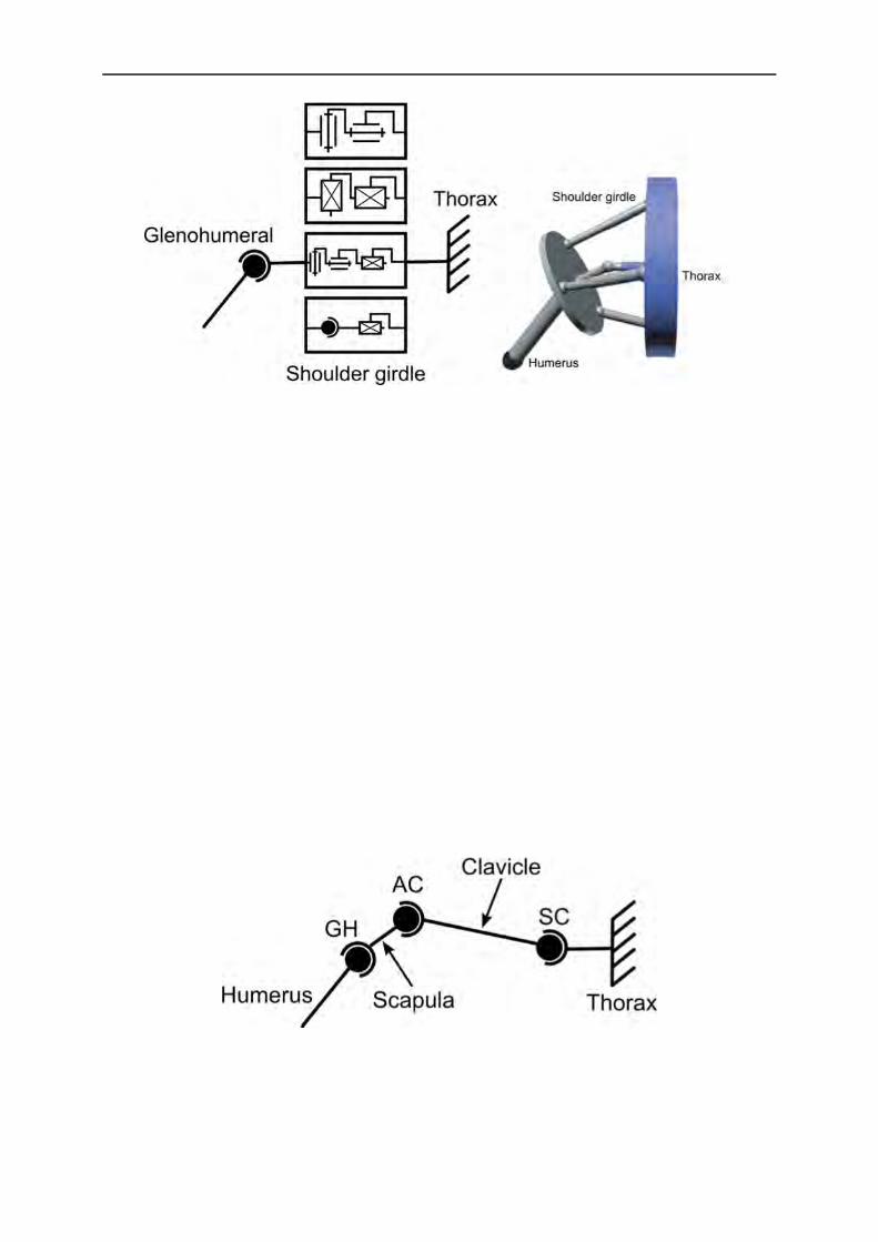
2.1.2. Shoulder girdle While several GH models have been discussed in the previous paragraph, the main differences when modelling the shoulder are due to the representation of the shoulder girdle composed by the scapula, the clavicle and the thorax. This closed chain allows positioning the GH joint in a correct manner and forming with this joint the shoulder complex. Shoulder girdle is composed of 2 true synovial joints: the sternoclavicular (SC) and acromioclavicular (AC) joints, completed by the scapulohoracic (ST) joint which is not considered as a true joint (i.e., no articular structure involved).
The SC joint (Figure 7) is the joint connecting the clavicle to the thorax through the manubrium and the cartilage of the first rib. This joint is commonly assimilated to a saddle joint as the two articular surfaces have a concave and convex torus shape. The torus shape could be assimilated as an inner tube. Consequently, mainly two DoF are allowed through this joint in the vertical and horizontal planes of the clavicle.
The AC joint (Figure 7) is composed of the scapula acromion and the lateral part of the clavicle. This joint allows rotation movements in the three planes but does not allow translation. This joint, due to small articular surfaces, is highly instable and prone to luxation. Its stability is mainly assumed by two external ligaments, the trapezoid and the conoid ligaments, positioned between the clavicle and the coracoid process.

Correction methods and models available
15
Figure 7 : Sternoclavicular and acromioclavicular joints (adapted from Netter (2006))
No articular structure is involved in the ST joint (Figure 8), this is why it is commonly not considered as a true joint. However, the movement of the scapula is constrained by the surrounding muscles to glide over the thorax above the serratus anterior and the subscapularis muscles.
Figure 8 : ScapuloThoracic joint in a coronal view (T3-T4) (adapted from Netter (2006))
2.1.2.1. Equivalent mechanism: first approximation for modelling shoulder girdle
The shoulder girdle can be firstly modelled as an equivalent mechanism representing the movements of the scapula and positioning correctly the GH joint (which, as it has been shown, is commonly modelled as a spherical joint). Different models of this kind can be found in the literature. Lenarcic and Umek (1994) and Malek et al. (Malek et al., 2006) used a simple universal joint while Yang (2005) used 2 prismatic joints. A more complex model was also proposed by Klopcar and Lenarcic (2006; 1999) where a universal joint was coupled with a prismatic joint. Finally, the universal joint was replaced by a spherical joint by Lenarcic and Stanistic (2003) (Figure 9). Alternatively, a robotic parallel mechanism has also been proposed by Lenarcic and Stanistic (2003).
Correction methods and models available
16
Figure 9 : Different equivalent shoulder girdle models (Lenarčič and Stanišić, 2003)
(adapted from (Sapio et al., 2006))
This latest model is a perfect example of equivalent model. With this robotic model, it is possible to have a precise positioning of the GH joint. However, it remains difficult to reobtain the proper kinematics of each bone of the shoulder girdle with such an approach. Consequently, all these models allow a simple representation of the phenomenon occurring in the shoulder girdle but do not allow a precise understanding of the different bones kinematics. They were mainly used as simplification for musculoskeletal models or for ergonomic studies (Malek et al., 2006; Yang et al., 2005) where the aim is to determine the reachable space of the upper limb. This approach seems thus limiting as the different scapular girdle structures cannot be studied separately.
2.1.2.2. Anatomical representation: Open loop vs Closed loop
Open loop model: Considering the different bony structures of the shoulder girdle
In an open loop mechanism (Figure 10), all the different bony structures of the shoulder girdle are considered. The thorax, the clavicle and the scapula are connected in pair by single mechanical links, mostly spherical joints (Engin and Tümer, 1989; Högfors et al., 1991; Yang et al., 2010).
Figure 10 : Example of an open-loop mechanism
Consequently, it is possible to obtain the complete kinematics of the different body segments, with a representation close to the anatomy. However, compared to the shoulder girdle equivalent

Correction methods and models available
17
mechanism which integrates indirectly the scapulothoracic constraints, this open loop model eludes it completely, which seems less physiological. Even if these models are easy to implement due to their simplicity, it could be interesting to consider the ST joint through the use of a closed loop model.
Closed loop model: Integration of the scapulothoracic joint
The closed loop model takes into account the ST joint controlling the scapula position relative to the thorax. The ST joint consists in a sliding of the scapula between different muscular and bursal planes. Consequently, the model allows representing a sliding movement composed of different rotation and translation movements. Therefore, the classical mechanical links are not used to represent this specific joint and are replaced by geometrical constraints. Commonly in the literature, this joint is considered as a contact between an ellipsoid representing the thorax and different points of the scapula (Maurel, 1995; Tondu, 2005) (Figure 11).
Figure 11: Shoulder girdle model considering scapulothoracic joint (Maurel, 1995) in (Yang et al., 2010)
Different models allowing three, four or five DoF have been proposed (Hill et al., 2008; Tondu, 2007) differing only by the number of contact points between the ellipsoid and the scapula (Figure 12). Thus, the three DoF model allows 2 translations and 1 rotation thanks to three contact points (Figure 12-c). By removing one contact point (Figure 12-b), one rotation is added. Finally, when only 1 point of contact (Figure12-a) is maintained, 2 translations and 3 rotations are allowed (Yang, 2003).
Figure 12: Different contact models of the scapulothoracic joint (Maurel, 1995) in (Yang et al., 2010)

Correction methods and models available
18
These models seem adapted as they allow all the DoF needed to represent the scapula movement. An important parameter in these models is the position of the contact points in the scapula. Commonly, one or two points of the medial border of the scapula are used (Garner and Pandy, 1999; Maurel, 1995; Tondu, 2005; van der Helm, 1994). Nevertheless, other points could be used as suggested by Sah and Wang (2009). Indeed, these authors found, through a cadaveric study, that the contact point between an ellipsoid representing the thorax and the scapula plane may be a point close to the barycentre of Angulus Inferior (AI), Angulus Acromialis (AA) and Trigonum Spinae(TS)(Figure 13).
Figure 13 : Scapula landmarks
Yet, considering that the scapula has a fixed contact point could be limiting. Indeed, sliding could occur on a fixed point on the thorax while the scapula is moving. Moreover, this geometrical model could theoretically allow the scapula intersecting the thorax which is not physiological. Indeed, the model constraints a scapula point to belong to an ellipsoid. As a result, the scapula could rotate freely around this point and intersect the ellipsoid modelling the thorax. A solution to this problem has been proposed in literature by imposing the scapula plane to be tangential to different geometrical surfaces. In Berthonnaud et al. (2005), the scapula was imposed to be tangential to a cone surface. For Maurel and Thalmann (1999), the thorax was assimilated to a sphere. This latest model seems the closest to the anatomical reality, although a sphere seems a too simplified representation of the thorax.
2.2. Forearm model: integration of a real pronosupination
The elbow joint allows connecting the humerus with the two bones (i.e, radius and ulna) of the forearm through the humeroulnar (HU) and humeroradial (HR) joints (Figure 14).

Correction methods and models available
19
Figure 14 : Forearm joints (adapted from Netter (2006))
The HU joint consists in the contact of the humeral trochlea and the trochlear notch of the ulna. This joint is commonly assimilated as a hinge joint allowing only flexion-extension movements. This is mainly due to the diabolo shape of the humeral trochlea and to the high adaptation of the trochlear notch of the ulna to this shape. This configuration tends to minimise or prevent any lateral movement and allows a good stability of the joint.
The HR joint connects the humerus capitulum to the radial head. However, if the joint would only be composed of these two elements, it would be strongly instable. A supplementary stabilisation is thus achieved by a contact between the radial head and the ulnar radial notch. Consequently, the radial head is articulated with both the humerus and the ulna. In addition, the radius is also connected distally with the ulna through the radioulnar joint (RU). This configuration allows the radius performing the pronosupination movement relative to the ulna and ensures a precise positioning of the hand which is connected to the wrist joint, allowing 2 rotations as DoF.
Consequently, the same question as for the shoulder girdle arises: could it be interesting to integrate these two bones in a closed loop kinematic chain? In simple models for motion analysis or musculoskeletal modelling, pronosupination has often been directly integrated in the elbow. A DoF in the axis of pronosupination is then added in the elbow joint in order to allow the flexion-extension and pronosupination movements. However, this model does not represent the complexity of the movement existing between humerus, ulna and radius.

Correction methods and models available
20
2.2.1. Simple model: Integration of the ulna and radius
The first model integrating the two bones in the forearm has been proposed by Fick (1904) (Figure 15).
Figure 15: Fick’s pronosupination model (1904)
In this model, the forearm is defined by two L-shaped elements connected with two spherical joints representing the radioulnar and the humeroradial joints. The ulna has only the flexion-extension rotation as DoF with the humerus. This model seems coherent with the elbow anatomy, but has an important issue: The parallelism between the elbow flexion-extension axis and the wrist flexion-extension axis cannot be conserved during a pronosupination movement (Kecskeméthy and Weinberg, 2005)(Figure 16).
Figure 16: Illustration of the unrealistic abduction of the hand during pronosupination with the Fick’s pronosupination model (Kecskeméthy and Weinberg, 2005)
As it can be seen on Figure 16, when the Fick’s model is used, an unrealistic adduction of the hand is observed. Consequently, this forearm model does not seem adapted to define a realistic upper limb kinematic chain.
2.2.2. Integration of a more realistic joint kinematic model: Lemay, Pennestri and Weinberg models
To manage this issue, there is a need to allow translation in the radioulnar joint as shown on Figure 17.

Correction methods and models available
21
Figure 17 : Illustration of the abduction and translation movement of the ulna and the compensation of the tilting (Gattamelata et al., 2007; Kecskeméthy and Weinberg, 2005)
Indeed, integrating additional DoF in the forearm model could improve the realism of Fick’s one (1904). Lemay and Cargo (1996) proposed thus a model allowing the axial displacement of the ulna (Figure 18)
Figure 18 : Lemay and Cargo’s (1996) forearm model
In this model, four body segments are defined: humerus, ulna, radius and hand. The humeroulnar joint is defined as a hinge joint allowing flexion-extension. The flexion-extension axis is defined as the axis from the HR joint centre to the trochlea centre. The HR joint is defined as a spherical joint allowing rotation in all directions such as in the Fick’s model. The proximal RU joint is directly integrated through the two previously described joint kinematic models. The main difference with the Fick’s model remains in the definition of the distal RU joint which is defined as a cylindrical joint. The axis of this cylindrical joint is defined as the axis going through the capitulum and the centre of the distal part of the ulna. This cylindrical joint allows the rotation and the translation of the ulna about the radius. Finally, the wrist model is a universal joint allowing 2 degrees of rotation. This simple joint model does not take into account the different carpal bones constituting the wrist joint. Nevertheless, this wrist model would be sufficient for an upper limb model mainly focusing on the shoulder complex and forearm kinematics, and not

Correction methods and models available
22
on the accurate description of the hand movements. Moreover, it is difficult, almost impossible, to measure the position of the different carpal bones using only cutaneous markers. A similar model was developed by Weinberg (2000) with the same DoF but with a different organisation of the joints (Figure 19). The aim was to represent the evasive motion of the ulna and the radius allowing the parallelism between the wrist and the elbow flexion-extension axes. In this model, the radius has distally a universal joint and proximally a prismatic joint. The ulna is connected proximally with a spherical joint and distally with a hinge joint.
Figure 19: Weinberg’s (2000) pronosupination model
As the Lemay Cargo and Weinberg models are 1 DoF systems, the position of the different body segments is known directly from the knowledge of the pronosupination angle (i.e., on Figure 19). Consequently, this model could be too restrictive for the MBO approach. A similar model has been developed by Pennestri et al (2007) (Figure 20). However, the radioulnar joint has been replaced by a guide instead of the cylinder in the Lemay and Cargo model. It thus allows 3 DoF in rotation and one DoF in translation.
Figure 20 : Pennestri’s model (adapted from Netter (2006))
This model seems more biofidelic as the different joints used better correspond to the anatomical joints (e.g., the guide joint used for the RU joint).
Hand Ulna
Radius
Elbow

Correction methods and models available
23
2.2.3. Integration of supplementary degrees of freedom.
The movement of the ulna is more complex than a simple flexion-extension movement relative to the humerus. Indeed, during pronosupination, the ulna describes an arc of circle composed of an extension followed by a lateral motion and finally a flexion relative to the humerus (Duchenne, 1949; Dwight, 1884; Heinberg, 1884). Two additional phenomenon are observed here: a ulna axial displacement and a swaying, which corresponds to an humeroulnar abduction-adduction movement (Gattamelata et al., 2007). As a result, it could be interesting to add these two DoF on the hinge HU joint in order to better represent its kinematics. These two DoF would be a translation in the direction of the hinge axis and a rotation in order to allow the humeroulnar abduction-adduction movement. However, as it has been highlighted previously, adding too many DoF can be deleterious to the MBO approach as the STA-related errors are partially corrected through the joint constraints. In addition, these two additional movements of the ulna are small compared to the main ones (flexion-extension and pronosupination). As a result, the Pennestri’s model seems a good compromise for the MBO method, as it integrates the two bones, represents well enough the forearm anatomy and seems constraining enough the system to minimise the STA-related errors.
These different forearm models will also allow taking into account one important parameter of the forearm: the carrying angle. The carrying angle corresponds to the angle that can exist between the humerus and the forearm in anatomical position (Figure 21). This can be taken into account by modifying the hinge joint axis in order to use this angle as a parameter of the model.
Figure 21: Illustration of the carrying angle (adapted from Netter (2006))
To conclude this part on the different joint kinematic models that can be used for the upper limb, it is important to note that integrating more bones and a more anatomical behaviour in our model can also be an important feature for further development. Indeed, implementing the different muscles to go towards a musculoskeletal model requires a correct positioning of all the

Correction methods and models available
24
bones during a movement (the muscles being attached on the bones), which is not accessible using the simplest models presented initially.
Choosing the joint kinematic model is an important point for the quality of the expected correction of STA related error. However, another parameter should be considered for the quality of the kinematic model: the model’s geometry and the different methods used to define it.
3. Geometric parameters The previously detailed joint kinematic models rely on a set of geometric parameters (e.g., axis and centre of rotation) having a significant impact on the results obtained. Indeed, if the different axes or centres of rotation are poorly positioned, the resulting models may not be able to reproduce the bone kinematics and correct for the STA.
3.1. Prediction methods
The prediction methods are the most commonly used methods for determining the geometry of the different joints due to their simplicity. No additional manipulation is needed than the basic motion capture protocol as they are based on the positioning of different cutaneous markers. Consequently, these methods can be easily integrated in a daily clinical routine for pathological patients. For example, the 7cm-method developed by Schmidt et al. (Schmidt et al., 1999) considers that the centre of the GH joint is positioned 7 cm below the top of the acromion and in the direction of the middle of the two elbow epicondyles (which is commonly described in prediction methods promoted by ISB recommendations as the centre of the elbow joint (Wu et al., 2005)). A similar method has been developed by Mackey et al. (2005) where the position of the GH centre is determined by two markers positioned on the anterior and posterior faces of the GH joint (Figure 22). On the other hand, axes are commonly defined as the direction between two cutaneous markers (e.g., ISB recommendations (Wu et al., 2002) propose defining the elbow flexion axis thanks to the medial and lateral epicondyles).
Figure 22 : Glenohumeral centre in the Mackey et al.’s method (2005)

Correction methods and models available
25
However, this method is not able to determine precisely the joint centre as it is only based on simple geometry rules and does not take into account the size or the morphology of the subject. These last elements can be taken into account through the use of regression methods.
3.2. Regression and scaling methods
A regression method takes into account some anthropometric measurements and markers position in order to adapt the location of the different joints centre to the subject. The centre is commonly defined as belonging to the longitudinal axis, such as in prediction methods, but the position is adapted as a defined percentage of the body segment length which allows an adaptation to the subject size (De Leva, 1996; Ferrari et al., 2008; Rab et al., 2002) (Figure 23)
Figure 23 : Example of a regression method for the upper limb (De Leva, 1996)
Other regression methods allow defining the centre or axis positions outside of the longitudinal axis and use a regression formula based on the position of different cutaneous markers such as the method defined by Meskers et al. (1998). In this method, the GH centre is defined from the position of bony landmarks of the scapula. Such methods are generally based on cadaveric measurements or imaging techniques (e.g., the regression of Meskers et al. was obtained from measurements on 36 cadavers).
Another method that can be used is the scaling method. In this method, a predefined geometry integrating the different joint centres is scaled using a set of external anatomical landmarks that are known both on the predefined geometry and on the subject. Consequently, the internal geometry can be adapted to any patient size. The more external anatomical landmarks are used, the more precise this technique is. The reference internal geometry can be obtained from imaging techniques performed on multiple subjects or cadavers. The scaling method can be interesting due to its global approach. Indeed, multiple joints can be determined in the same time resulting in a better adaptability on the complete kinematic chain. The position used to define the reference geometry is also crucial as it is needed that the subject and the reference geometry pose match

Correction methods and models available
26
in order to obtain a correct positioning of the different elements. If the reference geometry has some defects due to the positioning, it can be deleterious to the final result.
Anyway, these two methods lack of adaptability. Indeed, they are generally based on the study of a specific population (e.g., for cadaveric studies, the cadaver used is generally the one from elderly). As a result, errors can arise when a regression or scaling method is used on a population different than the one used for its definition. Therefore, using a method which is adaptable to each subject could be more interesting.
3.3. Functional methods
Estimating a joint centre or an axis of rotation is also possible through the motion of the subject. Indeed, using specific movements of the subject, the different parameters defining the joints can be derived. All the methods based on this principle are called functional methods. The different functional methods have been categorised in two types (Ehrig et al., 2006). The first type is based on axis (Gamage and Lasenby, 2002; Halvorsen et al., 1999) or sphere (Cappozzo, 1984; Ehrig et al., 2006; Halvorsen et al., 1999) fitting methods, where the joint centre or axis is optimised in order to fit the markers trajectories. The second type, defined as “coordinates transformation method”, is based on the definition of a segmental coordinate system (SCS) on each body segment. Indeed, instead of considering each marker individually, at least three markers are used to define a SCS for each segment. The axis or centre of rotation can be expressed in each segmental coordinate system and is supposed to be fixed in the others SCSs. As a result, it is possible to obtain its position by minimising for all recorded frames the distance between the centre or axes expressed in each SCS (Ehrig et al., 2007, 2006). These methods can be used on pathological subjects (e.g., patients with prosthesis or altered joints) conversely to prediction or regression methods as they are not based on data from healthy subjects but directly on the movement of the patients, even a passive one. However, functional methods tend to be sensible to the range of motion. Indeed, when the subject performs a movement with small amplitude, the determination of the axis and centre can be imprecise (Bell et al., 1989; Piazza et al., 2001). Consequently, the use of this method for pathological subjects with reduced range of motion (i.e., due to important spasticity or important muscular shortening) can be compromised.
3.4. Imaging techniques
Finally, imaging techniques can be used to obtain the precise geometry of the subject. These techniques are largely available in clinical environments as they are commonly used by clinicians as diagnosis tools. Imaging techniques create a two- (2D) or three-dimensional (3D) representation of the different internal structures of the body with almost no physical damage for the subject (Figure 24). In our case, the organs studied are the bones. As a result, by knowing the 2D or 3D representation of the bones, it is possible to define the different joint parameters based on the fit of geometrical shapes on bones characteristic features. For example, a sphere can
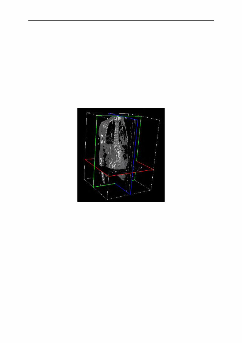
Correction methods and models available
27
be fitted on the humeral head and the centre of this sphere can be used as the GH joint centre. Imaging techniques can be divided in two main categories with ionising or non-ionising modalities (Hill et al., 2007). The main ionising techniques are based on the interaction of the matter with electromagnetic radiation and categorised as X-ray technology. It is possible to obtain a 2D static measurement of the bone through classical X-ray measurements. The CT-scan is based on the same technology and combines different X-ray images taken from different angles. The knowledge of different X-rays allows a 3D reconstruction. As a result, CT-scan creates a complete 3D representation of the skeleton of the subject of interest which allows a more precise kinematic chain modelling. However, these imaging techniques can be harmful for the human body as they are based on X-ray radiations (e.g., they can induce cancer and thus limit their use in a clinical routine context).
Figure 24 : Example of a 3D CT-scan images reconstruction (TurtelSeg)
New devices based on low dose radiation such as EOS allow obtaining a full 3D representation of the body (McKenna et al., 2012; Wybier and Bossard, 2013). EOS is based on the reconstruction obtained from only 2 images taken from 2 different planes. The use of the EOS system could be very interesting in a clinical routine as a full body acquisition can be done quickly with less risk than classical X-ray for the subject. It would allow determining the different internal joint parameters relative to external cutaneous markers positioned beforehand on the subject. However, in order to avoid any risk for the subject, even with low dose techniques, it will be preferred not to use these ionising techniques in clinic routine. In order to avoid this issue, other imaging techniques exist which are not based on the ionising radiation principle. For example, Magnetic Resonance Imaging (MRI) is based on the use of an electromagnetic field. Its interaction with the H2O molecules is measured and more particularly their polarisation which is different in function of the tissues. The use of a magnetic field instead of radiations allows an equivalent precision without any danger for the subject (Figure 25).

Correction methods and models available
28
Figure 25: MRI imaging of the forearm during a pronosupination movement (Nojiri et al., 2008)
If X-ray, MRI or other expensive devices can be used to obtain a precise definition of the different joints, some authors have proposed simpler and less costly methods. The use of ultrasound system techniques has been promoted as another simpler and less harmful imaging technique. They allow obtaining easily the representation in a plane of the different joints but can be difficult to manage for non-experimented users, and can be time consuming.
In any case, one limit can be raised: does joint centres or axes obtained through imaging techniques correspond really to the kinematic centre or axis of rotation? For example, is it better to use the GH joint defined thanks to functional methods based on a movement of the humerus or defining it as the geometric centre of the humeral head as it is done with imaging technique? Which one will give the best results when used with MBO techniques? Despite these latest interrogations, it seems that imaging techniques represent currently the best way to construct a joint kinematic model geometry that represents the subject anatomy.
4. Validation procedures To be able to use in a clinical daily routine the MBO correction method, joint kinematic models and geometries need to be validated. In order to be used as validation tools, the different measurement techniques must of course not be affected by STA.
4.1. Imaging techniques
The previously listed imaging techniques can be directly used for validation as, from the knowledge of successive bones positions, it will be possible to determine the bones kinematics. However, these techniques allow only obtaining static positions as the subject has to be motionless during the acquisition. Consequently, kinematics can only be approximated through multiple static acquisitions (called pseudo-kinematics). This can be a problem for example with X-ray based techniques since they will induce high radiation due to multiple acquisitions. Similar limitations are found when using EOS (a low dose X-ray system) for validation (Duprey et al.,

Correction methods and models available
29
2015) even if in that case the radiation are lower than classical X-ray based techniques. When 3D dynamic acquisitions can be made through the use of double fluoroscopy techniques (Figure 26), acquisition are limited to one joint due to the field of view size limitations. Moreover, in many cases, the subject is positioned in a tube where the range of motion is strongly limited. Even though some Open MRI exist for claustrophobic subjects or for having a better range of motion of the subject, they are rare and their use is often limited to medical purposes. Consequently, it seems difficult to perform a complete upper limb kinematic measurement with imaging technique due to the risk for the patient and the size limitations. Nevertheless, imaging techniques represent a good tool for validation and are often considered as silver standards.
Figure 26: Double fluoroscopy techniques (Boyer et al., 2008)
4.2. Palpation methods
Pseudo-kinematic acquisitions used in imaging techniques can also be used directly with an optoelectronic system as a validation method (Brochard et al., 2011; Lempereur et al., 2010b; Prinold et al., 2011). Indeed, if the subject is able to maintain his position long enough, an operator can palpate and digitise the different anatomical landmarks commonly by using a wand of known geometry and equipped with reflective markers. It is thus possible to get rid of the STA effects. This method is time consuming as each anatomical landmark should be pointed for each state of movement (up to 5 sec for each marker (Lempereur et al., 2010a)). Some tools that allow increasing the speed of pointing can be used. For example, the scapula locator allows digitising the complete scapula in one acquisition (Figure 27).
Figure 27: Scapula locator (Brochard et al., 2012)
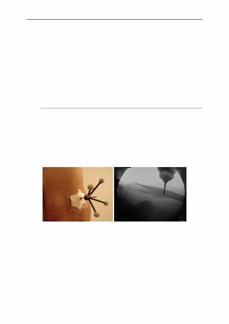
Correction methods and models available
30
However, these techniques are limited by the ability of the operator to determine correctly the position of the anatomical landmarks in a reproducible way. In addition, maintaining the position for the subjects can be difficult and they must thus mainly be in a lying position. Moreover, a bias can arise from the kinematic difference that exists between successive static positions and a dynamic movement. Indeed, the muscle activation patterns are totally different in both movements, and then a dynamic movement may not be the interpolation of the successive static positions. Nevertheless, quasi-static acquisitions using motion capture techniques represent a tool that is accessible and can be performed by any team already equipped with a motion capture system which is less expensive than any imaging system (which are generally not as accessible for research protocols as they are used for medical purposes).
4.3. Intracortical pins
One of the current gold standards for validation in motion capture is the use intracortical pins. In this method, after an incision of the skin, a hole is drilled in the bone allowing to position a screw/pins directly in the bone (Ludewig et al., 2009; McClure et al., 2011). A sensor or a cluster of markers is then rigidly secured to the pin (Figure 28). Consequently, the kinematics obtained is not affected by STA. The only errors could be due to the flexibility of the rod connecting the bone to the cluster which would bend during the motion or the skin limiting the movement of the rod due to a small skin incision.
Figure 28 : Example of intracortical pin ((Ludewig et al., 2009) on the right)
However, this technique cannot be used easily or commonly, even as a validation tool, as it is highly invasive and can result in pain during weeks for the subjects. For these reasons, these techniques are prohibited in many countries. As a result, very few studies are published using directly intracortical pins in vivo. Then, using intracortical pins on a cadaver can be considered as a compromise as there is no problem of invasiveness in that case. However, cadaveric experimentation can still be difficult to perform as the number of cadavers available is often low and the access to the facilities authorised to work with it difficult. In addition, one of the main limitations is that the movements have to be done passively. Indeed, a movement passively done might not represent the true active movement performed by a living subject. Nevertheless, if the

Correction methods and models available
31
cadaver is fresh or conserved correctly with no damage, it can still be used for the validation of the separated joint kinematics.
5. Thesis choices: Regarding the state of the art, it seems that the use of a MBO method with appropriate joint kinematic models (i.e., models that correspond to a description as close as possible to the anatomy) can be a good option to correct STA for the upper limb. In this thesis work, it has been chosen to use the following models. Firstly, the shoulder girdle will not be considered only as the GH joint, but as a complex joint comprising the clavicle, scapula and humerus. The focus will be mainly on the definition of an anatomical scapulothoracic joint. Different models will be integrated beginning with one or multiple points of the scapula being in contact with an ellipsoid representing the thorax. A new constraint that was never used before for correcting STA will also be developed. This new joint definition will constrain the plane defining the scapula to be tangent to the ellipsoid defining the thorax. Secondly, the forearm model will be an adaptation of the Pennestri’s model. This forearm model seems representing correctly the anatomy of the forearm as it integrates the radius and ulna and their different physiological joints. In order to validate these different models, an intracortical pins method will be used on cadaver and on in vivo subjects as this is considered as the current gold standard for measuring motion without any influence of STA.

32
Chapter 2
Theoretical background
The previous chapter introduced a multibody approach that will be used to correct soft tissue artefact (STA). Such an approach requires 1) defining the coordinate parameters used to position the segments of the kinematic chain, 2) establishing an optimisation procedure, and 3) defining the kinematic constraints of each joint. The parameters used to position the segments will yield the design variables of the optimisation. They also correspond to the different segment coordinate systems required to perform kinematics computation.
Contents 1. Natural coordinates and non-orthogonal coordinate system 32
2. Multibody system with natural coordinates ........................ 34
3. Upper limb model ............................................................... 35
3.1. Kinematics calculation ...................................................................................... 38
3.2. Virtual marker and vector definition ................................................................ 39
4. Multibody optimisation ...................................................... 40
4.1. Motor constraints .............................................................................................. 40
4.2. Rigid body constraints ...................................................................................... 41
4.3. Kinematic constraints ....................................................................................... 42
4.4. Final formulation .............................................................................................. 52
1. Natural coordinates and non-orthogonal coordinate system
Commonly in motion capture, either the relative coordinates or the absolute coordinates are used to define the position of the different body segments. In relative coordinates, each segment is defined relative to a previous one of the mechanism when in absolute coordinates each segment is positioned relative to a reference, generally representing the inertial coordinate system (ICS) if dynamic computations are also involved (Figure 29).

Theoretical background
33
Figure 29 : Plane mechanism parameterisation using relative coordinates (left)
and absolute coordinates (right)
However, introducing angles as the parameters to position the different body segments can result in a gimbal lock phenomenon and requires trigonometric functions during the kinematics computation. Gimbal lock occurs when 2 of the 3 axes allowing to position one body segment relative to another are aligned. In that case, the uniqueness of the solution is not respected. In addition, the equations expressing kinematic constraints using both coordinates systems imply an important number of trigonometric functions which are nonlinear. As a result, considering the gimbal lock phenomenon and the non-linearity of the equations, it can be difficult to solve, through the optimisation procedure, our multibody problem using either absolute or relative coordinate systems if angles are introduced. Consequently, it has been chosen to use a specific set of absolute coordinates: the natural coordinates (also called fully Cartesian coordinates).
Instead of using angles, which are likely to result in gimbal lock and leading to nonlinear trigonometric functions highly time consuming during the optimisation process, natural coordinates allow describing a segment position using only Cartesian coordinates of points and components of vectors. Indeed, in 3D, a segment can be described thanks to two points Pir and
Dir and two unit vectors iu and iw (Jalón et al., 1986; Jalón, 2007) (Figure 30). These entities
can be positioned on remarkable points, axes or planes of the defined mechanical joints. Twelve parameters are thus used to define the position of a body in a 3D space (i.e., four vectors with three components).
Natural coordinates can be difficult to implement but offer different advantages compared to the previously introduced parameters used to position the segments. Firstly, no angle is used. Consequently, the computation time is significantly reduced and the gimbal lock phenomenon (and the possible non-convergence issues associated to this phenomenon) is avoided when performing optimisation. Secondly, the position of each interesting anatomical point embedded in the segment can be easily obtained over time through the use of interpolation matrices giving the global coordinates of these points knowing the natural coordinates of the associated segments. These interpolation matrices are constant over time and may thus be defined prior to the
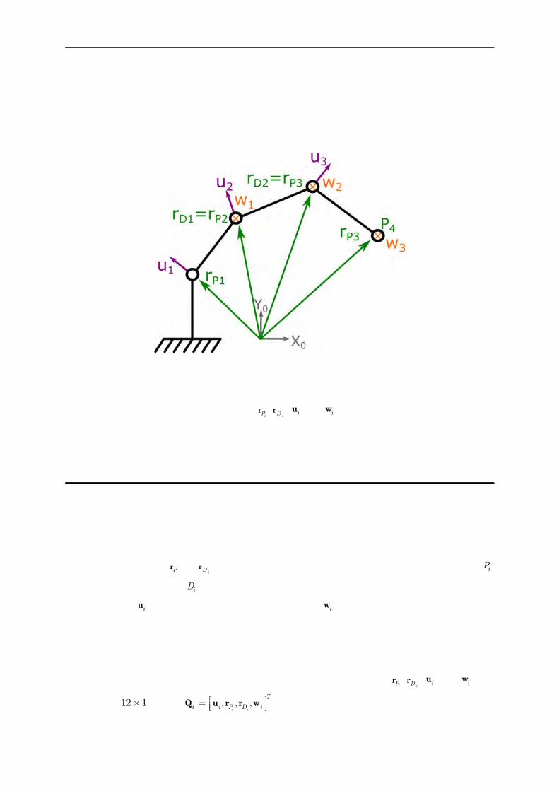
Theoretical background
34
optimisation process to increase the computation speed. Thirdly, natural coordinates allow simple expressions of joint constraints. Indeed, the equations defining a simple mechanical link rely only on points and vectors definitions and are always linear or quadratic which results again on a fast computation time, except when a complex geometry is integrated in the model as it will be seen later.
Figure 30: Plane mechanism parameterisation using natural coordinates
However, a post calculation is needed to obtain interpretable data for a clinical analysis that relies on classical Euler angles (even if
iPr ,
iDr , iu and iw can be associated directly to an
anatomical meaning). Yet, as the post processing of the data is less time consuming than the optimisation process, this latest problem should not be considered for the choice of a method for an optimisation procedure. Consequently, the natural coordinates will be used in this study.
2. Multibody system with natural coordinates The definition of the different body segments will be done through a multibody approach using natural coordinates. This will allow describing the position and orientation of a body segment using only two points
iPr et
iDr that will define the positions of the proximal joint centre iP
and the distal joint centre iD , and two unit directional vectors, the normal to the frontal plane
of the segment iu and the flexion axis of the distal joint iw (i being the number of the studied
segment in our model). This formulation has been proposed by Dumas and Cheze (2007) for studying the dynamics of the lower limb.
Each body segment position is reconstructed from motion capture data (i.e., 3D position of the cutaneous markers). The twelve parameters defining each segment (i.e.,
iPr ,
iDr , iu and iw ) are
held in the 12 1 vector , , ,i i
T
i i P D i
Q u r r w . Such a parameterisation allows defining a non-

Theoretical background
35
orthogonal segmental coordinate system (NSCS) with the non-orthogonal axes
, ,i ii i P D i
u v r r w and the origin at the proximal joint centre iP . It is thus possible to associate
the twelve parameters of iQ to the different anatomical planes or directions. In order to fully
define the segments, six rigid constraints are considered. For that, the distance iL between the
points iPr and
iDr , as well as the angles i , i and i between the 3 directions iu , iv and iw are
set constant. The geometric parameters , , ,i i i iL (Equation 2.1) can be determined from a
static image or using all the frames of a movement acquisition. In this latest case, mean value of
the geometric parameters , , ,i i i iL
are determined.
2
1
1
1
cos
cos
cos
i i
i i
i i
i P D
P D
i ii
i i i
P D
i ii
L
L
L
r r
r rw
u w
r ru
2.1
The kinematic chain can then be fully determined thanks to the vector 1, , , ,T
i n Q Q Q Q
containing the natural coordinates of the n body segments.
3. Upper limb model The upper limb system can be divided into seven bony structures: thorax, clavicle, scapula, humerus, ulna, radius and the hand (assumed rigid). As it has been described previously, the different SCSs are generally built using anatomical landmarks defined by the ISB recommendations (Figure 31 and Table 1). The definition of our different body segments using
natural coordinates , , ,i ii i P D i
Q u r r w can be found in the Figure 31 and the Table 2. As it can
be seen, the clavicle is not considered as a body segment in this MBO model. Indeed, it has been chosen to represent it as a kinematic constraint between the thorax and the scapula as it will be presented later in this chapter.

Theoretical background
36
Table 1 : The abbreviations of the different anatomical landmarks and their meaning (Wu et al., 2005)
Abbreviation Complete Name Localisation IJ Incisura Jugularis Deepest point of Incisura Jugularis PX Processus Xiphoideus Most Caudal point on the sternum C7 7th Cervical vertebra Processus Spinosus of the 7th cervical vertebra T8 8th Thoracic vertebra Processus Spinosus of the 8th thoracic vertebra SC Sternoclavicular joint Most ventral point on the sternoclavicular joint AC Acromioclavicular joint Most dorsal point on the acromioclavicular joint AA Angulus Acromialis Most laterodorsal point of the scapula TS Trigonum Spinae Scapulae Root of the scapula spine AI Angulus Inferior Most caudal point of the scapula EL Lateral epicondyle Most lateral point on lateral epicondyle EM Medial epicondyle Most medial point on medial epicondyle US Ulnar Styloid Most medial point on the ulnar styloid RS Radial Styloid Most lateral point on the radial styloid
MCP2 Metacarpophalangeal joint 2 (for the index/digitus secondus manus)
Most lateral point on the metacarpophalangeal joint of the digitus secondus manus
MCP5 Metacarpophalangeal joint 5 (pinky/digitus minimus manus)
Most medial point on the metacarpophalangeal joint of the digitus minimus manus
Figure 31 : The different upper limb bones and their associated landmarks (left) and parameters of the
upper limb using natural coordinates (right)

Theoretical background
37
Table 2: Upper limb construction of the parameters , , ,i ii i P D i
Q u r r w for each body segment
Segment Parameter Construction
Hand
1Pr
1 2P Dr r
1Dr Midpoint between the metacarpophalangeal (MCP) joints II and V
1u
1 1 1
11
P D r r w
uu
(note that 1 and 1 are equal to � 2� )
1w Vector pointing from MCP II to V.
Radius
2Pr Centre of the humeroradial joint (Head of the capitulum).
2Dr Centre of the wrist joint.
Midpoint between the ulnar styloid (US) and the radial styloid (RS)
2u
2 2 2
22
P D r r w
uu
(note that 2 and 2 are equal to � 2� )
2w Wrist flexion axis pointing laterally in anatomical position. ISB defines it as the vector pointing from the US to RS.
Ulna
4Pr
2Pr
3Dr Centre of the distal radioulnar joint
3u
3 3 3
33
P D r r w
uu
(note that 3 and 3 are equal to � 2� )
3w Elbow flexion extension axis pointing laterally in anatomical position
Humerus
4Pr Centre of the humeral head
4Dr
Centre of the elbow joint : The projection of the midpoint between the lateral epicondyle (EL) and the medial
epicondyle (EM) on the elbow flexion extension axis ( 4w )
4u
The vector pointing forward, perpendicular to the plane defined by the centre of the humeral head, EL and EM
4w Elbow flexion-extension axis pointing laterally in anatomical position. The direction of this axis can be obtained by functional method or by using EM and EL landmarks
Scapula
5Pr Most dorsal point of the AcromioClavicular joint (AC)
5Dr Centre of the glenoid fossa
5u
The vector pointing forward, perpendicular to the plane defined by the Angulus Acromialis (AA), the Trigonum Spinae Scapulae (TS) and the Angulus Inferior (AI). Note that 5 is equal to � 2�
5w The vector connecting TS to AA
Thorax
6Pr
Midpoint between Incisura Jugularis (IJ) and the spinous process of the 7th cervical vertebra (C7)
6Dr
Midpoint between the processus xiphoid (PX) and the spinous process of the 8th thoracic vertebra (T8)
6u
6 6 6
66
P D r r w
uu
(note that 6 and 6 are equal to � 2� )
6w The vector pointing to the right of the subject, perpendicular to the plane defined by IJ
C7, and 6Dr .
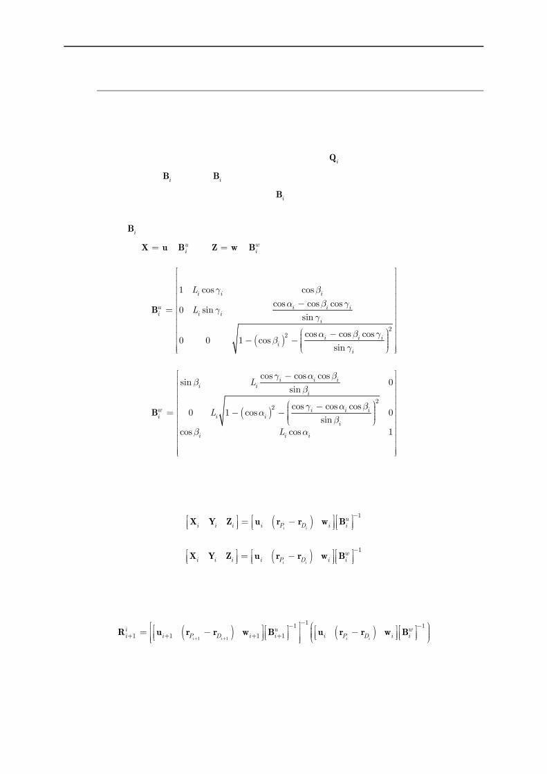
Theoretical background
38
3.1. Kinematics calculation
As it was described, the use of natural coordinates does not allow obtaining the definition of Euler angles directly interpretable in a clinical environment. However, the orthogonal segmental coordinate systems (SCS) defined by the ISB recommendations (Xi, Yi, Zi) can be easily reconstructed using a proper definition of the different iQ parameters and the following
transformation matrix iB . Matrix iB represents the orientation of the axes ui, vi, wi with respect
to the axes Xi, Yi, Zi of the SCS. Thus, matrix iB represents the choice made to align this SCS
with respect to the NSCS and which axes need to be redefined in an orthogonal way. In this way, two different iB matrices can be defined in function of the aligned vectors between SCS and
NSCS: assuming X u ( uiB ) or Z w ( w
iB )(Dumas et al., 2012; Duprey et al., 2010):
2
2
1 cos cos
cos cos cos0 sin
sin
cos cos cos0 0 1 cos
sin
i i i
u i i ii i i
i
i i ii
i
L
L
B 2.2
2
2
cos cos cossin 0
sin
cos cos cos0 1 cos 0
sin
cos cos 1
i i ii i
i
w i i ii i i
i
i i i
L
L
L
B 2.3
Each SCS can be then defined in order to perform further Euler angle calculations using one of the following relations:
1
i i
ui i i i P D i i
X Y Z u r r w B 2.4
1
i i
wi i i i P D i i
X Y Z u r r w B 2.5
Then, the rotation matrix from a proximal SCS to a distal SCS can be obtained using the following equation:
1 1
11 1
1 1 1 1i i i i
i u wi i P D i i i P D i i
R u r r w B u r r w B 2.6
Finally, the different rotation angles can be extracted from this rotation matrix using the adapted Euler sequence for each studied joint.

Theoretical background
39
3.2. Virtual marker and vector definition
The position of each marker (real markers placed on the skin or virtual markers representing the internal anatomy) can then be expressed using natural coordinates thanks to the previously defined NSCS and SCS. Indeed, the jiVi
un , jiVi
vn and jiVi
wn
coordinates of a marker j
iV in the
NSCS: , , ,i ii i i P D iP u v r r w can be obtained from a known position j
i
s
Vr expressed in the
SCS: , , ,i i i iP X Y Z thanks to the 1
ui
B matrix:
1
ji
ji
ji
ji
Vi
uV u si i VvVi
w
n
n B r
n
2.7
In a similar manner, it will be possible to define the components for any vector using the following formula:
1
ji
ji
ji
iu
u sji i i
v
iw
n
n
n
n
n B n
n
2.8
Where jiiu
nn , jii
v
nn and jii
w
nn are the components of the vector in the NCSC and sjin its
components in the SCS.
It is then possible to define the interpolation matrices jiViN and j
iniN allowing to obtain directly,
respectively the position of the point or the orientation of the vector, from the knowledge of iQ :
3 3 3 3 3 3 3 3 1j j j j ji i i i iV V V V Vi i i i i
u v v w
N n n n nE E E E 2.9
3 3 3 3 3 3 3 3
j j j j ji i i i in n n n ni i i i i
u v v w
N n n n nE E E E 2.10
Consequently, a virtual marker jiVr and a virtual direction sj
in can be expressed as a function of
the iQ parameters of their associated segment:
ji
ji
Vi iV
r N Q 2.11
jinj
i i in N Q 2.12
In order to differentiate the virtual markers (i.e., an internal point with a known position such as a joint centre) from the measured markers (i.e., the cutaneous markers positioned on the skin

Theoretical background
40
of the subject), two different namings will be used in the following chapters. Thus, jiVr and j
iViN
will be used for the virtual markers, while jiMr and j
iiMN will be used for the measured markers.
4. Multibody optimisation Once the SCS and the interpolation matrices of each segment are defined, an optimisation process can be applied to the multibody mechanism to take into account rigid body, kinematic and motor constraints. This optimisation consists in the minimisation of an objective function f x
depending on the design variables x under some inequality g x and/or equality h x
constraints:
min
0
0
f x
g x
h x
2.13
In this study, the rule of the function f x will be to minimise the distance between the measured
markers jiM
r and the model-determined corresponding markers jiM
i iN Q (i.e., f x represents the
so-called motor constraints). The design variables x correspond thus to the parameters
1 2 3 4 5 6, , , , ,T Q Q Q Q Q Q Q . The different equality constraints allow then defining the rigid body
constraints Φr and the kinematic constraints Φk representing completely our kinematic chain of the upper limb.
To solve this optimisation problem, the embedded function of Matlab, fmincon, has been chosen. The use of this function requires the definition of a cost function and constraint equations. Moreover, the value of the Jacobian of the different equations can also be given in order to decrease the calculation time. The following paragraphs aim thus defining the constraint equations Φ and their associated JacobianK .
4.1. Motor constraints
The objective function f x can be expressed as follows:
6 2
1 1
1
2
i ji
ji
mMi iM
i j
f
r N Q 2.14
where im is the number of cutaneous markers on the segment i . It would be possible to integrate
a weighting factor jiM
w in order to increase the influence of certain markers on which STA are
supposed to be less important. Initially, Lu and O Connor (1999) proposed to adapt the weighting factor based on the residual error artefact (difference between model determined and measured

Theoretical background
41
markers) which can correspond to the degree of STA. As shown by Begon et al. (2015), such a weighting should be adapted for each subject in order to improve the results, which is presently impossible without reference data such as imaging or intracortical pins. Consequently, it has been chosen to not use weighting factor in the objective function as its definition is still challenging. The factor ½ was used for an ease of use. It avoids to have factor after derivation when calculating the Jacobian. By introducing Φm , the vector of all the position errors of the cutaneous markers
jiM (i.e., the motor constraints), the objective function f can be rewritten as follows:
Φ Φ1
2
Tm mf 2.15
With :
Φ
11
11
11
11
16
16
66
66
1 1
1 1
6 6
6 6
m
m
m
m
M
M
M
Mm
M
M
M
M
r N Q
r N Q
r N Q
r N Q
2.16
For the motor constraints Φm , the associated Jacobian matrix mK depending on the iQ
parameters is:
11
11
12
22
55
1 3 12 3 12 3 12 3 12 3 12
1 3 12 3 12 3 12 3 12 3 12
3 12 2 3 12 3 12 3 12 3 12
3 12 2 3 12 3 12 3 12 3 12
3 12 3 12 3 12 3 12 5 3 12
3 12 3 12 3 12 3 12
0
m
m
m
M
M
M
Mm
M
N 0 0 0 0 0
N 0 0 0 0 0
0 N 0 0 0 0
K 0 N 0 0 0 0
0 0 0 0 N
0 0 0 0 0
16
66
3 12 6
3 12 3 12 3 12 3 12 3 12 6
m
M
M
N
0 0 0 0 0 N
2.17
4.2. Rigid body constraints
The rigid body constraints express the assumed non-deformability of the body segments. The rigid body constraints Φr
i of each body segment i is:

Theoretical background
42
Φ
2
22
2
2
1 0
cos 0
cos 0
0
cos 0
1 0
i i
i i
i i
i
i P D i i
i i iri
P D i
P D i i i
i
L
L
L
u
u r r
u w
r r
r r w
w
2.18
For the rigid body constraintsΦri , the associated Jacobian matrix r
iK depending on the iQ
parameters is:
3 1 3 1 3 1
3 1 3 1 3 1
3 1 3 1 3 1
3 1 3 1 3 1 3 1
2
2
2
i i
i i
i i
i i
i P D i
T i P D iri
i Pi D i
i P D
u r r w 0 0 0
0 u 0 r r w 0K
0 u 0 r r w 0
0 0 u 0 r r 0
2.19
4.3. Kinematic constraints
4.3.1. Scapulothoracic joint Different scapulothoracic models have been considered for this joint. Firstly, it has been considered that the scapula plane was tangent to an ellipsoid representing the thorax as it seemed that this constraint was the most physiological. The more classical model used for the scapulothoracic joint is a contact point model where one or multiple points of the scapula are in contact with the same ellipsoid. In order to compare our new joint model, tangential to an ellipsoid, with the contact point models, these last ones have been also integrated in the MBO.
4.3.1.1. Model tangent to an ellipsoid The full calculation of the constraint equation and Jacobian of this constraint can be found in Annexe 1. The scapula plane (displayed in cyan on Figure 32) will be constrained to have its normal unit vector equal to a normal unit vector of the ellipsoid at the tangent point (displayed in orange on Figure 32). The scapula plane can be defined thanks to two parameters: a point
belonging to this plane 15
15
5 5V
Vr N Q and the unit vector normal to the scapula plane, that is to
say 5u . The ellipsoid is defined thanks to the direction of the principal axes (A,B,C), the half
axis ellipsoid dimensions (a ,b ,c ) and the ellipsoid centre 26
26
6 6V
Vr N Q .
The associated kinematic constraint is then:
Φ2 16 5T
5 5 5 6 6 5 5* * * 0V Vk T
ST
u B u u N Q N Q 2.20

Theoretical background
43
Figure 32 : Scapulothoracic joint modelled as a plane tangent to an ellipsoid
Where B is the diagonal matrix containing the squared half axis ellipsoid dimensions (a ,b ,c ).
2
2
2
0 0
0 0
0 0
a
b
c
B 2.21
This equation is only valid when the different principal axes of the ellipsoid are parallel to those of the ICS. In order to be able to use any ellipsoid, it will thus be necessary to transfer this equation in the coordinate system of the ellipsoid.
Let us consider the rotation matrix R from the ellipsoid SCS to the ICS. A , B and C are the 3 directions of the principal axes of the ellipsoid and expressed by natural coordinates using the
three interpolation matrices 16
6nN
26
6nN and
36
6nN :
16
26
36
6 6
6 6
6 6
T
T
TT
T T
n
n
n
QA
R B Q
Q
N
N
NC
2.22
Consequently, the equation 2.20 can be rewritten:
Φ2 16 5
T
5 5 5 6 6 5 5* * * 0T V Vk
ST
Ru B Ru Ru R N Q N Q 2.23
Φ2 16 5T T
5 5 5 6 6 5 5* * * * * 0V Vk T
ST
u R B R u u N Q N Q 2.24
For the plane tangent to an ellipsoid, the associated Jacobian matrix kSTK depending on the Q
parameters associated to the joint constraint ΦkST is:

Theoretical background
44
Φ Φ Φ Φ Φ
1 12 1 12 1 12 1 125 5 5 5 6
k k k k kk ST ST ST ST STST
P D
K 0 0 0 0
u r r w Q 2.25
With:
Φ 26
1 1 15 5 5
53 3 6 6
5 5 5
5
5 5 5 3 3 5 (1:3,4:12) 51:3,1:3 1:3,1:3
5
* * **
* * * *
( ) * * *
k TVST
T
PV V VT
D
R B R uE N Q
u u R B R u
r
N N u E N r
w
2.26
Φ 1
55 5 (1:3,4:6)
5
kVTST
P
u N
r 2.27
Φ 1
55 5 (1:3,7:9)
5
kVTST
D
u N
r 2.28
Φ 1
55 5 (1:3,10:12)
5
kVTST
u N
w 2.29
Φγ
1 2 3 26 6 6 6
26 6 1 12 1 12
21 12 6 6 1 12
21 12 1 12 6 6
5 6 6 6 5 6T T6 65 5
1* * * *
2 * * * *
T
T
TkVTST
a
b
c
n n n
Q Q 0 0
0 Q Q 0
0 0 Q Qu N N N u N
Q Qu R B R u
2.30
With:
16
26
36
6
6 5
6
T
T T
T
n
n
n
N
U N u
N
2.31
γ
36 1 36 1 36 1 36 1
36 1 36 1 36 1 36 1
36 1 36 1 36 1 36 1
36 1 36 1
36 1 36 1 36 1 36 1 36 1
36 1 36 1 36 1 36 1 36 1 432 12
T
T
TT
T
T
U 0 0 0 0
0 U 0 0 0
0 0 U 0 0
0 0
0 0 0 0 U 0
0 0 0 0 0 U
2.32

Theoretical background
45
2 6 612 12 12 12
6
2 6 612 12 12 12
6
2 6 612 12 12 12
6
22 6 66 6 1 12 1 12
12 12 12 122 6
1 12 6 6 1 12
2 2 6 61 12 1 12 6 6 12 12
66
( * )
( * )
( * )
( * )
( * )
T
xT
xT
xTT
T yT
T
y
au
bu
cu
a aub
c bu
Q Q0 0
Q Q0 0
Q Q0 0
Q QQ Q 0 0 0 0
0 Q Q 0Q Q
0 0 Q Q 0 0
Q12 12
2 6 612 12 12 12
6
2 6 612 12 12 12
6
2 6 612 12 12 12
6
2 6 612 12 12 12
6
( * )
( * )
( * )
( * )
T
T
y
T
zT
zT
z
cu
aw
bw
cw
Q Q0 0
Q Q0 0
Q Q0 0
Q Q0 0
36 432
2.33
Each derivative 6 6* T
Q Q ( being the Xth parameter of 6Q ), corresponds to the addition of
two 12x12 matrices, the first one containing the vector 6TQ at the Xth row and the second one
containing 6Q at the Xth column. For example, the derivative associated with 6P xr (i.e., the 4th
parameter) is:
6
12 36 6
6 12 3 6 12 8
12 8
* T
T
P x
0Q Q
Q 0 Q 0r
0
2.34
4.3.1.2. Contact point model The scapulothoracic joint has been considered as a constraint imposing the plane of the scapula to be tangent to an ellipsoid representing the thorax but it can also be considered only as a
specific scapula point in contact with the same ellipsoid. Considering a scapula point 25
25
5 5V
Vr N Q
that is supposed to be in contact with the ellipsoid and the centre of the ellipsoid represented by 26
26
6 6V
Vr N Q , the associated kinematic constraint can be defined as:
Φ 2 2 2 25 6 5 6
1 0T
k TSC V V V V r r RAR r r 2.35
Φ2 2 2 25 6 5 6
5 5 6 6 5 5 6 6 1 0T
V V V Vk TSC N Q N Q RAR N Q N Q 2.36

Theoretical background
46
With
2
2
2
10 0
10 0
10 0
a
b
c
A and R being the rotation matrix from the ellipsoid coordinate system
to ICS. ellX ellY and ellZ are the 3 directions of the principal axes of the ellipsoid and can be
expressed by natural coordinates using the interpolation matrices 16
6nN
26
6nN and
36
6nN :
16
26
36
6 6
6 6
6 6
T
Tell TT
ell
T Tell
n
n
n
QX
R Y Q
Q
N
NZ
N
2.37
It is possible to extend the constraint to a model with two or three points in contact with an
ellipsoid by using the equation multiple times and modifying the point of contact 5
55 5
i
i
V
Vr N Q
used in the equation. For example for two contact points 25
25
5 5V
Vr N Q and
35
35
5 5V
Vr N Q , the
equation would become:
Φ
2 26 6
2 26 6
5 5 6 6 5 5 6 6
5 5 6 6 5 5 6 6
1 0
1 0
TV VT
kSC T
V VT
2 25 5
3 35 5
V V
V V
N Q N Q RAR N Q N Q
N Q N Q RAR N Q N Q
2.38
For the point in contact with an ellipsoid joint constraintΦkST , the associated Jacobian matrix
kSTK depending on the iQ is:
Φ Φ
12 1 12 1 12 1 12 15 6
T Tk SC SCSC
K 0 0 0 0
Q Q 2.39
With:
Φ 2 2 2
5 6 55 5 6 6 5
5
2T T
V V VTSC
N Q N Q RAR N
Q 2.40
Supposing being the Xth parameter of 6Q , the derivatives can be expressed as follows:
Φ 2 2 2 2 2 2 25 6 5 5 6 5 6
5 5 6 6 5 (1:3, ) 5 5 6 6 5 5 6 62 2T T T
V V V V V V VT T TSCX x
N Q N Q R ARN N Q N Q R AC N Q N Q
2.41

Theoretical background
47
61 12 1 12
61 12 1 12
61 12 1 12
Q0 0
QC 0 0
Q0 0
2.42
66 66 6 6 6P xy yx z zru wu u w
Q 2.43
So 6
Q is a matrix fully filled with 0 except for the parameter equal to . Consequently, it is
possible to obtain Φ
6
TSC
Q using the formula for each parameter.
Φ Φ Φ Φ Φ Φ Φ
66 6 6 6 6 6
T T T T T T TSC SC SC SC SC SC SC
x y z P x y zu u u r w w
Q
2.44
As for the constraint, the Jacobian for multiple contact points can be obtained by using the Jacobian associated with each contact point.
4.3.2. Clavicle Instead of considering the clavicle as a rigid segment connected by two spherical joints at the thorax and the scapula, it will be represented as a constant length between one point of the
thorax and one point of the scapula (Figure 33). Considering 16
16
6 6V
Vr N Q the centre of the
sternoclavicular joint, 25
25
5 5V
Vr N Q
the centre of the acromioclavicular joint and 1
Clavd the
constant length between the two centres, the kinematic constraint expressing the constant length between these two points is:
Φ1 16 5
6 6 5
2 2
15 0V Vk Clav
Clav d N NQ Q 2.45
For the constraint ΦkClav , the associated Jacobian matrix k
ClavK depending on the iQ is:
61 1 1 1
5 61 1
5 5 66 6 5 5 5 6 6 5 5 63 12 3 12 3 12 3 12 2 2V V V V V Vk
Clav 0 0 0 0 N N N N N NK Q Q Q Q 2.46

Theoretical background
48
Figure 33: Clavicle kinematic constraint modelled as a constant link between the thorax and the scapula
4.3.3. Glenohumeral joint Commonly, the glenohumeral joint is modelled as a spherical joint but it has been considered here as a link of constant length between the centre of the glenoid fossa and the humeral head centre in order to represent the translation movement that can exist between these structures (Figure 34).
Figure 34: Glenohumeral kinematic constraint modelled as a spherical joint (left) and as a constant link
between the centre of the humeral head and that of the glenoid fossa (right)
4.3.3.1. Case 1: Spherical joint When the glenohumeral joint is considered as a spherical joint (Figure 34), the associated kinematic constraint is then:

Theoretical background
49
Φ5 4
0kGH D P r r 2.47
In this equation, the distal point of a segment is assumed to be at the same position as the proximal point of the connected segment. The associated Jacobian matrix k
GHK depending on
the iQ is:
3 12 3 12 3 12 3 3 3 3 3 3 3 3 3 3 3 3 3 3 3 3 3 12kGH
0 0 0 0 0 0 0 0 0 0K E E 2.48
4.3.3.2. Case 2: Constant length When the glenohumeral joint is considered as a constant length between the glenoid fossa and the humeral head centres, if 1
5d is this constant length between the two centres (Figure 34), the
associated constraint equation is then:
Φ5 4
2
5
21 0k
GH D P d r r 2.49
The associated Jacobian matrix kGHK depending on the iQ is:
1 12 1 12 1 12 1 3 3 3 1 3 1 3 1 3 1 3 3 3 1 3 1 125 4 5 42 2
T T
D P DH P
k
G 0 0 0 0 r r 0 0 0 0 r r 0 0K E E
2.50
4.3.4. Forearm It has been chosen to model the forearm using the Pennestri et al.’s model (2007). Consequently, a spherical joint is used for the humeroradial joint, a hinge joint for the humeroulnar joint and a guide joint for the distal radioulnar joint.
4.3.4.1. Humeroradial joint The humeroradial joint is modelled as a spherical joint between a virtual marker attached to
humerus 14
14
4 4V
Vr N Q and the proximal point of the radius P2 (Figure 35).
The associated kinematic constraint is then:
Φ14
21 4 0Vk
HR P N Q r 2.51
The associated Jacobian matrix kHRK depending on the iQ is:
14
3 12 3 3 3 3 3 3 3 3 3 12 1 3 12 3 12Vk
HR E N
K 0 0 0 0 0 0 0 2.52
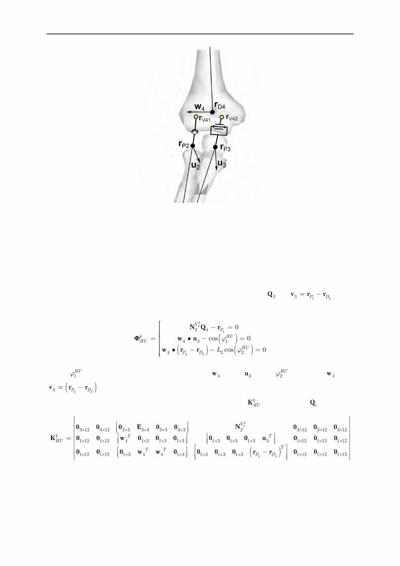
Theoretical background
50
Figure 35 : Elbow joint model comprising the humeroradial joint modelled as a spherical joint and the humeroulnar joint modelled as a hinge joint
4.3.4.2. Humeroulnar joint The humeroulnar is modelled as a hinge joint between the humerus and the ulna where the centre of the hinge joint will be positioned at P3 (Figure 35). It would be possible to use any point positioned on the rotation axis but this one is used in order to simplify the equation as it will allow having the direction of the pronosupination contained in the 3Q as
3 33 P D v r r . The
associated kinematic constraint is then:
Φ
24
3
3 3
2 4
4 3 1
4 3 2
0
cos 0
cos 0
VP
k HUHU
HUP D L
N Q r
w u
w r r
2.53
With 1HU being the constant angle between 4w and 3u and 2
HU between 4w and
3 33 P D v r r . These two angles can be defined from a static acquisition or from a complete
acquisition using mean value. The associated Jacobian matrix kHUK depending on iQ is:
24
3 3
3 12 3 12 3 3 3 3 3 3 3 3 2 3 12 3 12 3 12
1 12 1 12 4 1 3 1 3 1 3 1 3 1 3 1 3 3 1 12 1 12 1 12
1 12 1 12 1 3 4 4 1 3 1 3 1 3 1 3 1 12 1 12 1 12
V
k T THU
TT T
P D
0 0 0 E 0 0 N 0 0 0
K 0 0 w 0 0 0 0 0 0 u 0 0 0
0 0 0 w w 0 0 0 0 r r 0 0 0
2.54
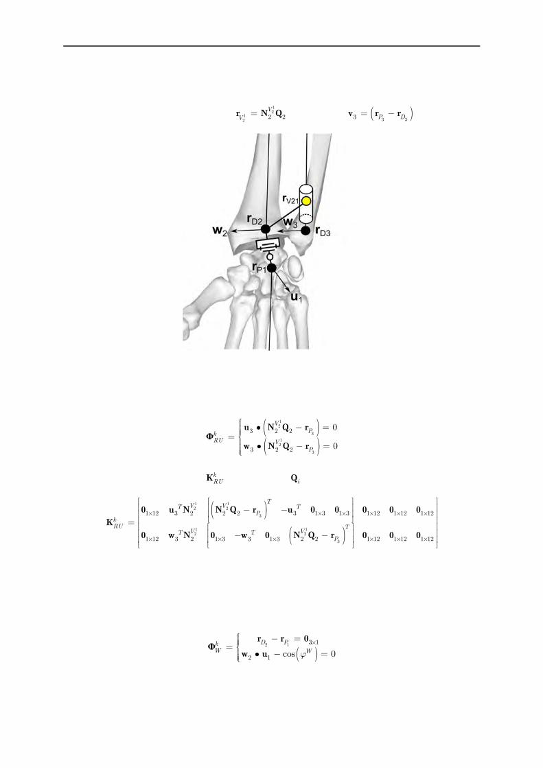
Theoretical background
51
4.3.4.3. Distal radioulnar joint The link connecting the proximal part of the ulna and the radius is considered as a guide joint
between a virtual marker of the radius 12
12
2 2V
Vr N Q and the axis
3 33 P D v r r (Figure 36).
Figure 36 : Distal radioulnar joint and wrist joint kinematic constraints recpectively considered as a guide joint and an universal joint
The associated kinematic constraint can be expressed as follows:
Φ
12
3
12
3
22
3 2
3
2
0
0
VPk
VU
P
R
N Q r
N Q r
u
w 2.55
The associated Jacobian matrix kRUK depending on iQ is:
1 12 2
3
1 12 2
3
1 12 3 2 2 2 3 1 3 1 3 1 12 1 12 1 12
1 12 3 2 1 3 3 1 3 2 2 1 12 1 12 1 12
TV VT T
PkRU T
V VT TP
0 u N N Q r u 0 0 0 0 0
K
0 w N 0 w 0 N Q r 0 0 0
2.56
4.3.5. Wrist The wrist connecting the radius and the hand is modelled as a universal joint (Figure 36). The associated kinematic constraint can be expressed as follows:
Φ 2 1 3 1
2 1 cos 0
D PkW W
r r 0
w u 2.57

Theoretical background
52
Where W being the constant angle between the two axes of the universal wrist joint. As for a
hinge joint, this angle can be fixed at 90°, but it can also be defined from the different Q parameters:
12 1cosW w u 2.58
In that case, the angle can be defined from a single static frame or by using the mean value W
obtained from a complete acquisition. The associated Jacobian matrix kWK depending on iQ is:
3 3 3 3 3 3 3 3 3 3 3 3 3 3 3 3 3 12 3 12 3 12 3 12
2 1 3 1 3 1 3 1 3 1 3 1 3 1 1 12 1 12 1 12 1 12
kW T T
0 E 0 0 0 0 E 0 0 0 0 0K
w 0 0 0 0 0 0 u 0 0 0 0 2.59
4.4. Final formulation
Finally our MBO problem can be written as follows :
Φ Φ Φ
Φ
ΦΦ
Φ
1min with
2
constrained to 0 with
Tm m m m
Q
r
kr r
k k
ff
KQ
K
Q K
2.60
With:
T
k k k k k k k kST clav GH HU HR RU W
K K K K K K K K 2.61
And:
1 6 12 6 12 6 12 6 12 6 12
6 12 2 6 12 6 12 6 12 6 12
6 12 6 12 3 6 12 6 12 6 12
6 12 6 12 6 12 4 6 12 6 12
6 12 6 12 6 12 6 12 5 6 12
6 12 6 12 6 12 6 12 6 12 6
r
r
rr
r
r
r
K 0 0 0 0 0
0 K 0 0 0 0
0 0 K 0 0 0K
0 0 0 K 0 0
0 0 0 0 K 0
0 0 0 0 0 K
2.62
We now dispose of an upper limb model that can be used in MBO in order to correct STA. In the next chapter, a cadaveric study will be conducted in order to validate this model.

53
Chapter 3
Cadaveric study
As it has been shown, the use of MultiBody Optimisation (MBO) should allow correcting Soft Tissue Artefact (STA)-related errors. One of the essential parameters for the correction efficiency is the joint kinematic models chosen. As a result, it will be necessary to test and validate the different models proposed and to determine the closest one to the bones kinematics. For this purpose, obtaining the true kinematics of the different body segments is necessary. One of the solutions is to avoid STA through the use of intracortical pins which can be done on cadaveric pieces (Fung et al., 2001; Kasten et al., 2004; Matsumura et al., 2013). The other parameters determinant for the model’s quality, and hypothetically for the correction level that can be obtained, are the geometric parameters of the different joints kinematic models (e.g., centres of rotation, axes position or the parameters defining the ellipsoid modelling the thorax). Accurate geometric parameters should also allow improving the definition of the kinematic constraints. Currently, in the literature, these parameters are extracted from different imaging technics or cadaveric studies, which means from different subjects or cadavers. Consequently, it could be difficult to obtain a complete and correct construction of a MBO model of the entire upper limb. In addition, when complete data from an entire body are available, such as in the Visible Human Project (Ackerman, 1998; Garner and Pandy, 1999, 2001), the posture of the body (from which the data should be extracted) can be problematic. Indeed, in this project, a cadaver was frozen in a gelatine and traverse sections of 1mm throughout the entire body were taken and compiled in order to construct a precise representation of the inside of the human body. For that, the cadaver was in a lying position on his back without any muscular passive resistance when he was immobilised which could result in a specific positioning of the different body segments. In that case, scapulae were pushed on the thorax which did not represent the position that would take these segments in a upright posture. This could have been avoided by positioning the body in the anatomical reference position. Consequently, based on a fresh cadaver immobilised in a vertical anatomical position, our experimentation aimed at:
1) Measuring precisely the true kinematics of the different body segments in order to validate the joint kinematics models and the ability of MBO to mimic human motion.
2) Obtaining geometric parameters of the complete upper limb kinematic chain and compare the results obtained from different scaling parameters construction methods
Intracortical pins associated with reflective markers can be used with a motion capture system based on optoelectronic cameras in order to obtain the bones kinematics of the upper limb. These data could then be used to fulfil the first aim of this study. In addition, motion capture can also be used to obtain geometric parameters through palpation methods for external landmarks, or

Cadaveric study
54
through functional methods for internal landmarks. As functional methods should be more accurate with intracortical pins as STA does not alter the recorded movements, they should allow obtaining more precise geometric parameters. However, all these parameters cannot be obtained using motion analysis. It is then necessary to use imaging technics to access other parameters. As a result, in order to validate the joint kinematic models and obtain the correct geometric parameters, an experimental protocol combining motion analysis on a cadaver with intracortical pins and a CT-scan has been achieved.
Contents 1. Experimental protocol ........................................................ 54
1.1. Cadaver preparation ......................................................................................... 54
1.2. Motion capture protocol ................................................................................... 57
1.3. CT-scan ............................................................................................................. 58
1.4. Model generation............................................................................................... 59
1.5. Models comparison ............................................................................................ 61
1.6. Contact point .................................................................................................... 62
2. Results ................................................................................ 65
2.1. Scapulothoracic joint ........................................................................................ 65
2.2. Forearm ............................................................................................................. 72
3. Discussion ........................................................................... 73
3.1. Scapulothoracic model ...................................................................................... 73
3.2. Forearm model .................................................................................................. 77
4. Limits ................................................................................. 77
5. Conclusion .......................................................................... 78
1. Experimental protocol
1.1. Cadaver preparation
One fresh frozen human cadaver (97 years old) was stored at -20°C and thawed 24 hours before experimentation in the anatomy laboratory of the CHU of Caen. Removal of the skin was necessary in order to reduce the rigor mortis limitation of the movement and facilitate the
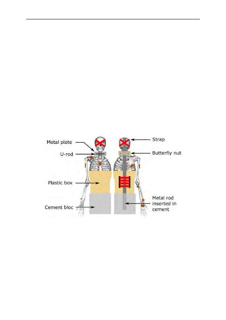
Cadaveric study
55
intracortical pins positioning. A full body was available but the lower limbs were removed due to technical constraints. In first guess, it would have been interesting to record the motion of the cutaneous markers in order to evaluate the ability of the model to correct STA. However, it was impossible to glue the cutaneous markers on the skin of the cadaver. Even if it would have been possible to sew the cutaneous markers on the skin, as a cadaver was used, the motion of the surrounding tissues would not represent the skin motion in an active movement of a normal subject. As a result, it was thus chosen not to measure STA on the cadaver.
The cadaver torso was rigidly fixed vertically (Figure 37). For this, a vertical metal rod locked in a cement bloc was used. The lower part of the cadaver torso was inserted in a plastic box which was rigidly fixed to the metal rod allowing to maintain this part of the cadaver motionless. The neck was maintained motionless using a fixation system composed of a U-threaded rod, a small metal plate with two holes and two butterfly nuts. The U-threaded rod was positioned around the cadaver neck with its two ends inserted in the metal plate. The metal plate was positioned in the other side of the metal rod to compress the threaded rod on the neck using the two butterfly nuts. In order to avoid any disturbing head movement, additional straps were used around the head to stabilise the cadaver.
Figure 37 : Fixation device allowing to maintain the cadaver during motion capture
Once the cadaver was positioned correctly on the fixation device, the clusters of reflective markers were fixed rigidly on the body segments. Several parameters have been considered when choosing the position of the clusters. Firstly, it has been chosen to position them as far as possible from joints. The aim was to avoid any imaging artefact when using the CT-Scan. Indeed, the metal contained in the screw could disturb the images obtained. Consequently, if screws were closed to a zone of interest, some information could have been erroneous or lost. Secondly, the bone resistance was taken into consideration. In order to ensure a good fixation of the screws in the bone, it has been chosen to implant them in the strongest part of the bone. The definition of these positions was validated by an experienced orthopaedic surgeon.

Cadaveric study
56
Finally, it has been avoided to position any cluster on the anterior part of the cadaver not to damage the clusters during transportation and CT-scan acquisition. Indeed, during these tasks, the cadaver was positioned lying on the anterior part of the thorax. If any cluster was damaged or moved during these tasks, it would have been impossible to use the data obtained from the CT-scan for the motion analysis as their position regarding to the associated bone would not be the same. This procedure has been respected for every bone except for the thorax and clavicle. For the thorax, the cluster was fixed in the sternum as mobility can exist between the different vertebrae. In order to protect the cluster during transportation and CT-Scan acquisition, a wood box has been made to protect the cluster from any contact. This box was larger and higher than the cluster in order to allow the thorax to be in support on the box instead of the cluster. For the clavicle, as the trunk was in contact with the wood box during transportation it was impossible for the clavicle cluster to be in contact with the surfaces and then be damaged.
The clusters on which the reflective markers were positioned had a size of 6.5×4.5×2.3cm. They were made of wood and fixed to the bones thanks to 2 screws that were positioned in their middle. Four reflective markers where fixed on them using a wooden glue (Figure 38).
Figure 38 : Triangular and rectangular clusters of reflective markers
A triangular version of the clusters, with only three markers, was also designed for the ulna and radius as less space was available for the cluster’s positioning (Figure 38). Considering the fixation constraints discussed previously, it was chosen to use the following clusters positioning (Figure 37) associated with the drilling described in Table 3.
As it can be seen (Table 3), the ulna cluster was positioned on the proximal part of the ulna. A triangular cluster was used in order not to restrict the pronosupination movement. This cluster was positioned in order to have a side aligned with the ulna and the apex pointing medially. Similarly, a triangle cluster was also used for the radius. It was positioned distally on the radius and the apex was pointing laterally. This positioning of the two forearm clusters avoided any contact between the two clusters and did not restrict pronosupination movements.
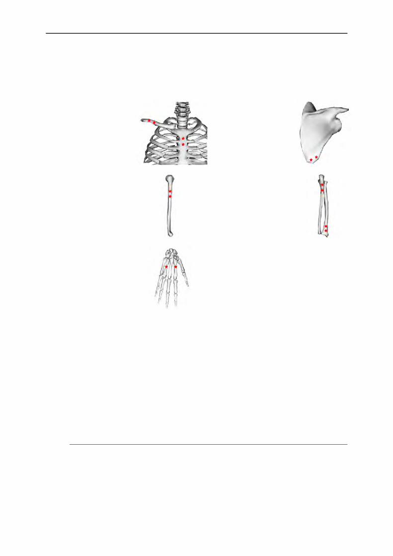
Cadaveric study
57
Table 3 : Drill points positioning on the different body segments
Body Segment
Position Drill Point (indicated by red
star)
Body Segment
Position Drill Point (indicated by red
star)
Thorax Below the manubrium
Scapula Inferior lateral border
Clavicle Distal part of the
clavicle
Humerus Laterally to the deltoid insertion
Ulna Proximal part of the ulna
Radius Distal part of
the radius
Hand In the metacarp in the back of the hand
The skin of the cadaver was completely removed of the whole body surface prior to fix the clusters. Then, the clusters were fixed to the body in two steps. Firstly, the surrounding tissues (e.g., muscles) were incised in order to have a direct access to the bones. This was done in order to avoid the drill bits to be stuck in the soft-tissues. Small holes were prepared in the bones in order to facilitate the screwing and avoid any bone fracture or degradation that could result in a movement between the bone and the cluster. In addition, wood screws were used to avoid bone fracture. The cadaver did not present any scars indicating probably no history of surgical procedure or damage on the upper limb susceptible to alter the kinematics. This was confirmed latter thanks to the CT-scan measurement.
1.2. Motion capture protocol
Movements of the right side of the cadaver were recorded using eight optoelectronic cameras (OQUS, Qualysis AB, Sweden) sampled at 100Hz. A static capture was performed in order to point the position of the different anatomical landmarks (including ISB landmarks locations (Wu et al., 2005)) in the corresponding SCSs. Indeed, it was not possible to stick the reflective markers on the skin during movements acquisition as the skin was removed, but the knowledge of the

Cadaveric study
58
landmarks position was essential to reconstruct the different SCSs from their position in the technical coordinate system (i.e., CAST method (Cappozzo et al., 2005)). The cadaver movements were generated by an experimenter who was moving the different body segments. Different movements have been chosen that can be divided in two categories: functional movements and validation movements. On one hand, functional movements were performed as they allow obtaining geometrical construction parameters that can be used for the definition of the MBO model. For the GH centre, the movement recommendations of Lempereur et al. (2010b) were followed. Then, three consecutive abduction-adduction, flexion-extension and circumduction movements were performed in an amplitude of 30° for all DoF. For the forearm, elbow flexion-extension and pronosupination (with the elbow flexed at 90°) movements were performed. On the other hand, validation movements were composed of a classical set of basic movements for the shoulder. Three repetitions of full flexion, extension, abduction and circumduction movements were thus performed. Moreover, three repetitions of reaching back movements were also added as a movement of the daily life. The functional movements used for the determination of the geometrical construction parameters were also considered as validation movements. The different movements performed are summarized below (Table 4).
Table 4 : Summary of the validation movements
Shoulder
Functional movements (Lempereur et al., 2010b)
Full flexion-extension
Full abduction-adduction
Full circumduction
Forearm Elbow Flexion-extension (functional movement)
Pronosupination (functional movement)
Daily life movement Reaching back
All data were transferred to Matlab R2011b using the Biomechanical ToolKit (BTK) (Barre and Armand, 2014) for computations. For each movement, the position of the landmarks were reconstructed in order to obtain the , , ,
i ii i P D i
Q u r r w parameters (Chapter 2 paragraph 2) for
the body segments.
1.3. CT-scan
The aim of this part was to obtain the geometrical construction parameters from a CT-scan acquisition in the anatomical reference posture. These parameters comprised the position of the
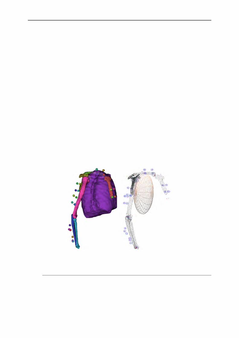
Cadaveric study
59
different joint centres, the functional axes and the position and shape of the ellipsoid modelling the thorax. As the different reflective markers were visible in the CT-scan, it was possible to position the geometric parameters and the anatomical markers in the clusters technical coordinate systems allowing thus a precise registration of the different body segments in the data obtained during the motion capture measurements.
The cadaver was frozen in the anatomical reference posture just after the motion analysis measurements to ensure the preservation of this position in the CT-scan in a lying posture. For that, the cadaver was kept in the posture thanks to the metal rod with straps and placed in the anatomical laboratory freezer during 24 hours prior to the CT-scan acquisition. For this acquisition, the cadaver was removed from the metal rod and put in a ventral position. A particular attention was paid on the clusters of markers in order to avoid any damage or displacement.
The radiographic images were acquired using a CT-scan (Scanner General Electric Health Care, Optima 660 pro, Milwaukee, USA) (120kvp, 245mA). The acquisition was performed using the helicoidal mode with a 0.625mm slice spacing, a 50 cm diameters field of view with a plane resolution of 0.977x0.977 mm, which was the highest resolution available. Bone geometries were then reconstructed using a semi-automatic segmentation freeware (TurtleSeg) and data were transferred to Matlab using the MeshLab toolbox to extract the geometry of interest (e.g., the spherical surfaces of the humeral head) (Figure 39).
Figure 39 : 3D reconstruction in TurtleSeg (left) and in Matlab (right)
1.4. Model generation
In clinical context, it is difficult to obtain the internal geometry using imaging technics in daily routines. Indeed, as it has been suggested in Chapter 1, these methods are time consuming and can be harmful for the subject. The definition of the geometric parameters can then be difficult. One of the method that can be used to obtain these parameters is thus to scale an internal

Cadaveric study
60
geometry known from several studies to the subject anatomy. In order to evaluate the errors that might appear during clinical routines when the model is not personalised, it was necessary to compare the results obtained considering a precise geometry (obtained by CT-scan) and a scaled one. As the Visible Human Project (National Library of Medecine) (Ackerman, 1998; Garner and Pandy, 1999, 2001) is one of the most precise cadaver reconstruction freely available and accessible to every single laboratory, it has been chosen to use it in this study.
The reconstructed body segments were the thorax, the clavicle, the scapula, the humerus, the ulna and the radius. Different geometric elements were then extracted from this 3D reconstruction. Firstly, all the centres of the reflective markers were reconstructed and positioned in order to define each SCS and then to be able to transfer the information extracted from the CT-scan in the motion capture data. Secondly, all the ISB anatomical landmarks were located on the reconstructed bones. All the geometrical construction parameters were then extracted using similar definitions as for the Garner and Pandy model (1999) except for the ellipsoid and the sternoclavicular joint :
- The ellipsoid representing the thorax was built using the superior dorsal part of the reconstructed thorax using an ellipsoid fitting method. Consequently, only the functional part (i.e., the one where the scapula is in contact with the thorax) was used instead of trying to fit the entire lateral part of the thorax.
- The centre of the sternoclavicular joint was defined as the centre between the middle of the two articular surfaces in contact. Indeed, it seemed difficult to fit a sphere on the end of each bone (particularly on the manubrium).
- This later approach was successfully used for the acromioclavicular joint where it was possible to apply a sphere fitting method on the bones extremity.
- The glenoid fossa and humeral head were obtained using a sphere fitting on the articular surfaces. The flexion-extension axis of the elbow was determined using a cylinder fitting method on the articular surfaces of the distal part of the humerus.
- The capitulum centre and the distal head of the ulna were finally defined as the centre of their respective articular surfaces.
Two MBO models were then generated. The first one was based on the geometry of the Visible Human Project scaled to model geometry (Garner and Pandy, 1999, 2001) scaled to our cadaver for the shoulder complex and based on functional methods for determining the parameters necessary to the forearm closed loop model. The second model was only based on the CT-scan data (Table 5). These models were applied for each recorded movement.

Cadaveric study
61
Table 5 : Origin of the different geometrical construction parameters used for the 2 compared models
Shoulder complex Joint Model 1: Scaling Model 2: CT Model Anatomical landmark Pointed using reflective marker Pointed on CT-scan data SternoClavicular (SC) Scaling from visible Human CT-scan data AcromioClavicular (AC) Scaling from visible Human CT-scan data GlenoHumeral (GH) Functional CT-scan data Ellipsoid Scaling from visible Human CT-scan data
Forearm Joint Model 1: Functional Model 2: CT Model Elbow flexion-extension axis Functional CT-scan data Capitulum centre Functional CT-scan data Distal ulna head centre (allows defining pronosupination axis) Functional CT-scan data
Wrist Marker-based Marker-based
Four scapulothoracic models of contact with an ellipsoid modelling the thorax were considered: 1) one contact point between AI and TS (ST1a), 2) one contact point which was the barycenter of AI, TS and AA (ST1b), 3) two contact points AI and TS (ST2) and 4) tangent to an ellipsoid (STT). Contact points positions were defined during a static acquisition where the previously listed points were projected on the ellipsoid modelling the thorax. A similar approach was used for the definition of the point belonging to the plane tangent to an ellipsoid. This point was chosen as the point of the ellipsoid where both the ellipsoid and the scapula plane (defined by AI, TS and AA) have the same normal vector in the static position, which allowed having initially this plane tangent to the ellipsoid.
Two forearm models were considered. The first one was the forearm closed loop model (Chapter 2 paragraph 4.3.4). The second one was composed of an universal joint connecting the forearm to the humerus (i.e., the simplest and commonly used model when estimating the elbow kinematics (Prokopenko et al., 2001; Roux et al., 2002; Schmidt et al., 1999; Wu et al., 2005)). As clusters were positioned on both ulna and radius, it was necessary to determine in the latter case from which cluster the forearm motor constraints would be defined. As only the radius is involved in the flexion-extension and the pronosupination movements, the radius was assimilated as the forearm. Consequently, the second model consisted in the humerus connected to the radius through a universal joint.
1.5. Models comparison
It has been chosen to compare the accuracy of the different models using the error existing between the bones kinematics (determined using intracortical pin markers) and the one obtained using MBO for different kinematic models for all the studied movements. Box plots of the error

Cadaveric study
62
were used to obtain a concise representation of the error distribution. They were completed with the Root Mean Square Error (RMSE) associated to the coefficient of determination (R2) as goodness-of-fit indicators (Figure 40). The correlation levels were defined as follows: 0≤R2<0.3 was defined as low correlation, 0.3≤R2<0.6 a medium correlation, 0.6≤R2<0.9 a high correlation and 0.9≤R2 a very high correlation.
Figure 40 : Box plot definition
To compare the scapulothoracic models, the kinematics in the three DoF (i.e., upward-downward rotation, protraction-retraction and anterior-posterior tilt) was used. For the forearm models, the elbow flexion-extension and pronosupination were considered. However, the universal model did not integrate the ulna in the optimisation procedure contrary to the closed loop forearm model. Consequently, the definition of the forearm kinematics (i.e., flexion-extension and pronosupination movements) had to be defined in a similar manner for both models. Thus, it has been chosen to use the radius as an equivalent forearm for the kinematic comparison. ISB recommendations were followed for all kinematic computations.
1.6. Contact point
1.6.1. Definition From here, a clear difference must be made between two concepts:
- Contact point,
- Constraint point.
In the Chapter 2, a model described as a contact point on an ellipsoid has been defined for representing the scapulothoracic joint. The point used in these constraints was not a point of the scapula plane but a projection of this point on the ellipsoid according to the normal to the scapula plane during the static acquisition in the reference anatomical posture. It was needed to project this point on the ellipsoid in order to obtain a physiological constraint. Indeed, it would have been impossible for the posterior part of the scapula (where the anatomical landmarks were located) to be in contact with the ellipsoid representing the thorax during a movement. Consequently, the points of the scapula were projected on the ellipsoid in order to represent the

Cadaveric study
63
anterior part of the scapula which can physiologically be in contact with the thorax ellipsoid (Figure 41). These constraint points are fixed in the scapula SCS and are used as kinematic constraints (i.e., constraint points). However, these constraint points are different from the contact points between the ellipsoid and the scapula.
From an anatomical point of view, defining the contact point between the thorax and the scapula could be difficult. From a mechanical point of view, this point could be considered as the point of minimal distance between the scapula and thorax bones. However, it was impossible to obtain such a precise representation and the two bony structures were simplified. Indeed, in our model, the thorax was assimilated to an ellipsoid and the scapula to a plane. As a result, the definition of a contact point between the two structures became the ellipsoid point of minimal distance between the scapula plane and the thorax ellipsoid. The plane tangent to the ellipsoid at this contact point has the same normal as the scapula plane. If a plane of similar normal was defined using the different constraint points (i.e., the specific scapula landmark projected on the ellipsoid), they would almost automatically intersect the ellipsoid as shown on Figure 41.
Figure 41 : Schema (left) of the projected point on the ellipsoid modelling the thorax and its associated plane and the representation extracted from the data (right)
Consequently, the constraint point corresponded to the point used as kinematic constraint and the contact point to the ellipsoid point of minimal distance between the scapula plane and the ellipsoid (Figure 42).
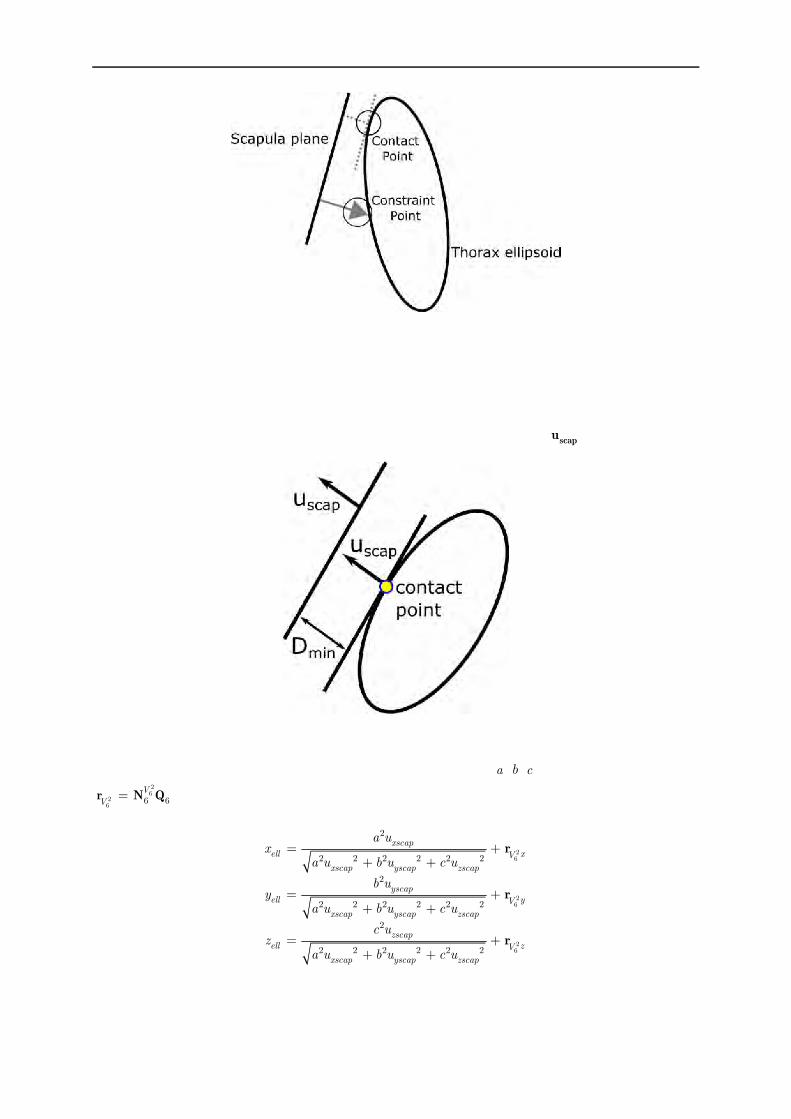
Cadaveric study
64
Figure 42 : Difference between the contact point and the constraint point
1.6.2. Equation The ellipsoid point of minimal distance between the scapula and the thorax, so called “contact point”, corresponded to the ellipsoid point where the normal is equal to scapu (Figure 43).
Figure 43 : Contact point definition
For an ellipsoid defined by the half axis ellipsoid dimensions (a ,b ,c ) and the ellipsoid centre 26
26
6 6V
Vr N Q , the contact point coordinates in the ISC were given by the following equations:
26
26
26
2
2 2 2 2 2 2
2
2 2 2 2 2 2
2
2 2 2 2 2 2
xscapell xV
xscap yscap zscap
yscapell yV
xscap yscap zscap
zscapell zV
xscap yscap zscap
a ux
a u b u c u
b uy
a u b u c u
c uz
a u b u c u
r
r
r
3.1

Cadaveric study
65
However, these equations were only valid when the different principal axes of the ellipsoid were parallel to those of the ICS. In order to be able to use any ellipsoid, it was thus necessary to transfer this equation in the ellipsoid SCS. Let thus consider the rotation matrix R from the ellipsoid SCS to the ICS. A , B and C are the 3 directions of the principal axes of the ellipsoid
expressed by natural coordinates using the three vector interpolation matrices 16
6nN ,
26
6nN , and
36
6nN :
16
26
36
6 6
6 6
6 6
T
T
TT
T T
n
n
n
QA
R B Q
Q
N
N
NC
3.2
So, instead of using the scapu vector in this equation, the vector uscapRu was used. This contact
point has then been plotted for each movement, for the reference data, and when using the different MBO models.
The contact point between the scapula plane defined by the three landmarks AA-AI-TS (normal vector scapu ) and the ellipsoid were then plotted in the scapula SCS for the different geometries
and movements previously described.
2. Results
2.1. Scapulothoracic joint
2.1.1. Kinematics The following paragraphs are related to the scapulothoracic kinematics obtained using intracortical clusters as motor constraints on the different scapulothoracic joint kinematic models with different geometries (Figures 44 to 49).
In the following part, the nomenclature of the name of the models follows the rule: Geometry-Model (e.g., CT-ST1a for a model constructed with the geometry extracted from the CT-scan using the scapulothoracic kinematic model ST1a, or Sca-ST2 for a model constructed with the scaling geometry using the scapulothoracic kinematic model ST2).

Cadaveric study
66
Figure 44 : Boxplots of the errors existing between the bones kinematics and the different models’ kinematics for the anterior-posterior tilt, the upward-downward rotation and the protraction-retraction
during an abduction movement.
Figure 45 : Boxplots of the errors existing between the bones kinematics and the different models’ kinematics for the anterior-posterior tilt, the upward-downward rotation and the protraction-retraction
during a circumduction movement.

Cadaveric study
67
Figure 46 : Boxplots of the errors existing between the bones kinematics and the different models’ kinematics for the anterior-posterior tilt, the upward-downward rotation and the protraction-retraction
during an extension movement.
Figure 47 : Boxplots of the errors existing between the bones kinematics and the different models’ kinematics for the anterior-posterior tilt, the upward-downward rotation and the protraction-retraction
during a flexion movement.

Cadaveric study
68
Figure 48 : Boxplots of the errors existing between the bones kinematics and the different models’ kinematics for the anterior-posterior tilt, the upward-downward rotation and the protraction-retraction during a functional movement of the shoulder (e.g., movement composed of flexion-abduction-rotation
and circumduction).
Figure 49 : Boxplots of the errors existing between the bones kinematics and the different models’ kinematics for the anterior-posterior tilt, the upward-downward rotation and the protraction-retraction
during a reaching back pocket movement.

Cadaveric study
69
The use of different joint kinematic models for the scapulothoracic joint did not seem impacting the results obtained when a similar geometry is used. Indeed, the RMSE between the scapulothoracic models with the same geometry was always below 3°. Lower errors between MBO and bones kinematics were found when the CT-scan geometry was used instead of the Scaling geometry for the protraction-retraction and the anterior-posterior tilt. When the Scaling geometry was used, the range of error for protraction-retraction was higher than for anterior-posterior tilt. For upward-downward rotation, no difference could be observed between the different models regardless of the model and the geometry.
2.1.1.1. Upward-downward rotation The error obtained for the upward-downward rotation was low with a maximum RMSE of 1.77° and a maximum error of 4°. Except for movements with a low range of motion of upward-downward rotation (e.g., extension or functional shoulder movements), the MBO kinematics was highly correlated to the bones one for upward-downward rotation. For extension movement, the correlation between the bones and MBO kinematics was low to medium and medium to high for the functional movement. Except for these two last specific movements, upward-downward rotation was the DoF with the highest range of motion with an amplitude up to 40.25°.
2.1.1.2. Protraction-retraction For the protraction-retraction, when Scaling geometry was used, RMSE values vary from 4.67° up to 8.51° and a maximum error value around 12° could be found. The use of the CT-scan geometry allowed reducing the RMSE range from 0.62° to 4.97° and the maximum error to 8°. If ST1b and ST2 models were not considered, the range of RMSE with Scaling geometry became [6.13°; 8.51°] with a maximum error of 9°. With CT-scan geometry, the RMSE range became [0.62°; 2.81°] with a maximum error of 5°. Indeed, these two models resulted in higher errors for specific cases (e.g., CT-ST1b model during the abduction movement or Sca-ST2 during functional shoulder movement). The correlation between the MBO and the reference kinematics was always high to very high except for three specific cases during abduction movement where the correlation was medium (i.e., CT-ST1a: R2=0.30, Sca-ST1a: R2=0.30, and Sca-ST2: R2=0.55).
2.1.1.3. Anterior-posterior tilt Considering anterior-posterior tilt, the use of the CT-scan geometry allowed reducing the RMSE range from [2.06°; 6.43°] to [0.43°; 3.52°] and the maximum error from 12° to 8°. If ST1a model was not considered, the range of RMSE with Scaling geometry became [0.43°; 2.46°] with a maximum error of 9° and the RMSE range with CT-scan geometry was [0.62°; 2.81°] with a maximum error of 5°. Except for the two movements with a low anterior-posterior tilt amplitude (i.e., abduction and flexion), the correlation between the MBO and the bones kinematics was always high to very high. For the abduction and flexion movements, the anterior-posterior tilt correlation was low to medium.

Cadaveric study
70
2.1.2. Contact point The following paragraphs are related to the contact point obtained using intracortical clusters as motor constraints on the different scapulothoracic joint kinematic models with different geometries (Figures 50 & 51). When using the CT-scan geometry, it seemed that there was a low difference between the bones and models kinematics when considering the position of the contact point (Figure 51). By contrast, when the Scaling geometry was used (Figure 50), a difference in the contact point position between the bones and MBO kinematics can be found. Globally, for some specific movements and for both geometries, different patterns might be found between the different MBO models. However, the contact point was globally positioned in the same area associated with a specific ellipsoid geometry: around the AI landmark for the CT-scan geometry, and around the barycentre of AI, TS and AA for the Scaling geometry. For the tangent to an ellipsoid constraint, all the points were contained in the same plane due to the constraint definition while a variation in the depth relative to the surface of the ellipsoid was found for all other models.
Figure 50 : Contact point trajectories obtained with the different scapulothoracic models in the scapula SCS for all the recorded movements with the scaling based geometric parameters (Posterior view only).

Cadaveric study
71
Figure 51 : Contact point trajectories obtained with the different scapulothoracic models in the scapula SCS for all the recorded movements with the CT-scan based geometric parameters
(posterior and medial views).

Cadaveric study
72
For all movements, the contact point trajectories in the scapula SCS seemed to be different and associated with a specific movement of the scapula. Indeed, the trajectory pattern for each movement seemed to be repeated for each repetition of the movement. This phenomenon was particularly visible for the data obtained from the model constructed with CT-scan data where the amplitude of the contact point’s trajectory was greater. In addition, the patterns found for basic movements could be observed in more complex movements. For example, the reaching back movement had a similar pattern than the extension, or the flexion and abduction movements’ also had a similar pattern than the circumduction movement. For some movements with high upward-downward rotation amplitude (i.e., abduction, circumduction and flexion), the contact might be found outside the scapula.
2.2. Forearm
The following paragraphs are related to the forearm kinematics obtained using intracortical clusters as motor constraints on the different forearm models with different geometries (Figures 52 & 53).
Figure 52 : Boxplots of the error existing between the bones kinematics and the different models kinematics for the flexion-extension of the radius and the pronosupination of the radius for a flexion-
extension movement of the elbow.

Cadaveric study
73
Figure 53 : Boxplots of the error existing between the bones kinematics and the different model kinematics for the flexion-extension of the radius and the pronosupination of the radius for a
pronosupination movement.
On the whole, except for the Universal model based on Scaling geometrics parameters, results were similar regardless of the scapulothoracic kinematic model and the geometrical construction parameters used.
Regarding the flexion-extension movement, RMSE was low with a maximal value of 1.48°, and the correlation was always very high. The maximum error was obtained for the forearm closed loop model with functional geometric parameters.
Regarding the pronosupination movement, RMSE was also low, except for the Universal model with functional based geometric construction parameters (4.63°). The correlation was always very high. However, the amplitude of the error was higher than during flexion-extension movement, with a maximum amplitude of +/- 10°. In particular, it could be observed that this amplitude was higher when CT-scan based geometric parameters were used.
3. Discussion
3.1. Scapulothoracic model
3.1.1. Kinematics It seems that the choice of the ellipsoid geometry has a low impact on the upward-downward rotation obtained. Constraining the scapula being tangent to the ellipsoid modelling the thorax,

Cadaveric study
74
or the projection of specific scapula points being in contact with the ellipsoid, mainly impacts the direction of the normal to the scapula. Consequently, the rotation around this axis, which corresponds to the upward-downward rotation, was mainly constrained by the motor constraints instead of the kinematic constraints. As motor constraints were not affected by the STA in our experiment, the reference upward-downward rotation could be respected in both cases. In addition, the upward-downward rotation was the main DoF as it had the greater amplitude. Consequently, the motor constraints might impact more the resulting kinematics for this DoF. For some movements, low R2 were found for the upward-downward rotation but they were always associated with a low amplitude. However, a good correlation rarely appeared when the amplitude was really low (i.e., below 6°), and these results should not be considered to evaluate the quality of the different models.
No important difference was obtained using the different scapulothoracic joint kinematic models. The main improvement in the ability of the model to mimic the bones kinematics was the use of CT-scan construction geometrical parameters. The use of a personalised geometry allows a better representation of the movement when using MBO (Andersen et al., 2009; Reinbolt et al., 2005). It was initially hypothesised that the use of more physiological joint constraints would allow better mimicking better the kinematics. However, the use of the tangent to an ellipsoid constraint allowed only obtaining similar results than the common scapulothoracic models.
3.1.2. Contact point As it can be seen, the contact point is moving in the scapula SCS regardless of the scapulothoracic kinematic model used. Which means that even with a constraint imposing the projection of a specific point of the scapula to be on the surface of the ellipsoid, the contact point is moving. In a first thought, it would have been expected to have a fixed contact point when using a fixed constraint point model. However, this was due to the confusion that can exist between the contact and constraints points concepts (paragraph 1.6.1).
The constraint points are then linked to the scapulothoracic kinematic model and are fixed in the scapula SCS, while the contact points are linked to the scapula kinematics and can move regardless of the scapulothoracic joint model used. It then explains the moving contact point in scapula SCS obtained with the fixed constraint points. As it can be seen on the formula 3.1, the position of the contact point on the ellipsoid is mainly defined by the normal to the scapula plane and the ellipsoid parameters. Different constraint points allowed obtaining similar kinematics and then similar normal vectors to the scapula. In that case, similar trajectories of contact points were obtained although different constraint points were used. However, the reason why the contact point trajectory was similar was not due to the fact that the constraint point was fixed but because the kinematics was correctly represented. Only one model allows merging the constraint and contact points: the plane tangent to an ellipsoid model (Figure 54). Indeed, for the constraint point kinematic models, the applied constraint was at the position of the projected point. Conversely, for the plane tangent to an ellipsoid, the constraint was at the contact between

Cadaveric study
75
the plane and ellipsoid which then also corresponded to the contact point between the two structures.
Anyway, the use of the tangent to an ellipsoid scapulothoracic model did not impact the ability of the model to mimic the bones kinematics. However, the model seemed more adapted for further developments such as musculoskeletal modelling. Indeed, in order to obtain a correct skeletal dynamics, the contact point must be correctly defined. By modifying the contact point, the different muscular lever arms and thus the musculo-tendon forces estimations could be altered. In addition, this model seemed more adaptable as it could be able to replicate potential pathological scapula movements such as winging scapula (i.e., the contact between specific point of the scapula and the thorax can be lost), which is not the case for the models with constraint points. It must be noted that this equivalence between the contact and constraint points was only due to the definition of the plane tangent to an ellipsoid constraint. Indeed, the formula used for the definition of the contact point was one of the basic formula for the definition of the plane tangent to an ellipsoid constraint equation. However, it seemed coherent to use the definition formula of the contact point as a base for the constraint in order to obtain a more realistic upper limb kinematic model.
Figure 54 : Difference between constraint and contact points for the “tangent to an ellipsoid” and “contact point” kinematic constraints
3.1.3. Ellipsoid definition The use of different ellipsoid geometries resulted in a difference in the contact point trajectory (i.e., global position, pattern and amplitude). The coordinates of this point were linked to the kinematics obtained (i.e., a similar kinematics induces a similar contact point) and were around the initial contact point defined in the static position. Indeed, for a determined ellipsoid, the direction of the normal to the scapula plane defines directly the position of contact. As the orientation of this vector varied around its initial position, the contact point also varied around its initial position. The difference in the initial position was mainly due to the difference in the ellipsoid parameters (i.e., size, centre and orientation) between the CT-scan and the Scaling-based ellipsoids (Figure 55).

Cadaveric study
76
Figure 55 : Ellipsoids obtained from scaling method (red) and from the CT-scan data (blue) for two different orientations of the right upper limb
The difference in amplitude of the contact point trajectory between the two geometries was due to the curvature of the ellipsoid around this initial contact point. A lower curvature radius resulted in a higher variation of the contact point position for a similar variation of the normal vector as illustrated in the Figure 56.
Figure 56 : Variation of the contact point between a plane and an ellipse for two different radii
As it can be seen on the Figure 57, the contact on the Scaling ellipsoid was located on the upper part of the ellipsoid whereas it was located on the lateral part for CT-Scan ellipsoid. The curvature was then more important for the scaling ellipsoid contact point area than for the CT-scan contact point area. It thus explained the wider movements of the contact point with the CT-scan model.
This difference in the ellipsoid parameters (i.e., centre, axes radius and orientation) was due to the fact that in the Visual Human Project, the ellipsoid aimed fitting the complete lateral part of the thorax (Garner and Pandy, 1999), whereas in our model it has been chosen to use only the functional part of the thorax. In this study, this functional part has been chosen to be the dorsal superior part of the thorax resulting then in a smaller ellipsoid. Consequently, it is not the same ellipsoid defined by scaling or imaging techniques that is compared, but two different definitions of the ellipsoid. Nevertheless, it seemed that the definition of the ellipsoid might be determinant for the validity of the kinematics and the contact point obtained with the different models and should then be investigated in more details.

Cadaveric study
77
Figure 57 : Contact point position in the thorax SCS during a circumduction for the Scaling based geometry (red) and the CT-scan based geometry (blue)
3.2. Forearm model
Contrary to the scapulothoracic models, the use of CT-scan did not improve the quality of the results obtained with the forearm models. It actually tended to give worst results than functional methods. The forearm closed loop model improved the ability of the model to replicate the bones kinematics as the errors were low for any geometry used. As the bones kinematics was well replicated in all cases, it could be considered as a good model for the forearm. Moreover, as both the kinematics of the ulna and radius were considered, this model was also interesting as a first step towards the definition of a musculoskeletal model. It must be highlighted that the universal model did not take into account the ulna movement in the optimisation procedure as the radius was directly considered as the forearm in the model. Consequently, more motor constraints were used when the optimisation was done using the forearm closed loop model as both the markers positioned on the ulna and the radius were considered. Indeed, in the closed loop model, two additional kinematic constraints and three additional motor constraints were considered resulting then in more equations to solve. In first thought, it would be more difficult to obtain better results with the forearm closed loop model. Indeed, with more constraints, it is more difficult for a defined a mechanism following any movements (i.e., all the cadaver movements admissible). But as the bone kinematics is well replicated with this closed loop model, the different constraints used are valid and are thus more likely to correct STA-related errors. Thus, having more constraints should allow obtaining a better correction of STA-related errors with MBO, as in the proposed closed loop model.
4. Limits This study was limited by the fact that only one cadaver has been used for the validation. It could have been interesting to experiment the model on more movements and more cadavers.

Cadaveric study
78
For example, the forearm model could have been evaluated for pronosupination at different flexion angles to test if a greater error could be found for specific cases. Having more daily activities movements for the scapulothoracic joint kinematic validation could also have been interesting in order to confront the different models to multiple cases. In addition, as the measurements have been made on a cadaver, the bones kinematics obtained might be erroneous as the scapulothoracic joint is mainly positioned thanks to muscle constraints. This is not true for the forearm as the humerus, ulna and radius are mainly constrained by bone shapes and ligaments. The scapulothoracic model definition and evaluation was also limited by the ellipsoid definition. It would have been interesting to investigate different thorax ellipsoid definitions and more particularly to use a similar approach than in the Visible Human Project (Garner and Pandy, 1999, 2001). Indeed, the different observed effects might be more related to the definition of the ellipsoid than to the personalisation.
5. Conclusion The first goal of this chapter was to evaluate the ability of different models to mimic the bones kinematics of the scapulothoracic and the forearm joints. The two models that were integrated (i.e., tangent to an ellipsoid for the scapulothoracic joint and closed loop model for the forearm) allowed obtaining equivalent results than the former models when the ability to mimic the bones kinematics for the upper arm was evaluated. It seemed that the scapulothoracic models were more sensible to the geometric parameters. However, although these two models did not improve (nor reduce) the ability to mimic the bones kinematics, they allowed obtaining more information in a clinical perspective, and seemed necessary for the development of advanced musculoskeletal models of the upper limb. The tangent to an ellipsoid scapulothoracic constraint allowed equivalence between contact and constraint points contrary to the other scapulothoracic joint kinematic models. Consequently, even if the bones kinematics was replicated equally for all scapulothoracic models, the tangent to an ellipsoid model seemed to be more anatomical and thus allows a more interesting definition of the contact point for further dynamic calculation. The improvement for the forearm was obvious as both ulna and radius were considered with the forearm closed loop model.
The ability of the different models to mimic the bones kinematics has been evaluated here and good results were obtained for the new scapulothoracic and forearm kinematic models. This is a first step toward the design and validation of an upper limb MBO model. The next step was to evaluate the ability of MBO based on these models to reduce STA-related errors. As it was impossible to evaluate this information during this cadaveric study, the upper limb model has been confronted to in vivo intracortical pins data on voluntary healthy subjects. This study is presented in the next chapter.

79
Chapter 4
In vivo intracortical experimentation
In the previous chapter, the ability of the different joint kinematic constraints to mimic the bones kinematics has been evaluated through a cadaveric study. This step was the first in the development and validation process of a MultiBody Optimisation (MBO) model that could be used for correcting Soft Tissue Artefact (STA) related errors. Indeed, the use of a kinematic model that could not mimic the movements of the different bones should result in an insufficient or erroneous correction of STA-related errors. It has been shown that the different scapulothoracic kinematic models, compared in Chapter 3, are equally able to reproduce the bones kinematics, but their ability to correct STA-related errors has not yet been evaluated. The bones kinematics can be obtained through different methods but collecting both the kinematics of the bones and the one perturbed by STA is challenging. Indeed, it is necessary to measure simultaneously the bones movements and the cutaneous landmarks displacements during a dynamic acquisition in order to properly assess STA movements. Consequently, the use of palpation methods or imaging technics is compromised.
One solution would be to use intracortical pins implanted into the bones, as it is considered as the gold standard for measuring the bones kinematics (Bourne et al., 2007; Ludewig et al., 2009). In the previous chapter, this method has been used on a cadaver without measuring the STA. Actually, even if it would have been possible to stick markers on the skin, the STA would not have been representative of those of a living being. Consequently, the validation data could only be obtained by using intracortical pins on a living subject. In addition, data collected for STA correction on living subjects allows obtaining a more realistic kinematics of the scapula as its position and rotation are mainly driven by muscular contractions (Terry and Chopp, 2000). In the previous chapter, the scapula kinematics was obtained from a cadaver animated by an experimenter which might lead to somewhat incorrect scapula kinematics.
The use of in vivo intracortical pins measures represents thus one of the best validation data available for such a MBO model. Access such data would yet allows:
- Evaluating more precisely the ability of the different scapulothoracic kinematic models to mimic the bones kinematics on a living subject.
- Evaluating the ability of the different MBO models to correct STA
- Defining and evaluating a simpler correction method that could also allow correcting STA

In-vivo intracortical experimentation
80
However, as using intracortical pins is highly invasive, justify its use to an ethical committee, even on a low number of subjects, can be difficult. Consequently, these data are rare and difficult to obtain. In order to get such validation data, a collaboration has been established with the S2M lab (Montréal, Canada). Data from in vivo intracortical pins experiments (performed in Sweden) were thus shared in order to be used as validation data in this study.
Contents
1. Validation data ................................................................... 81
1.1. Intracortical pins ............................................................................................... 81
1.2. Comparison method .......................................................................................... 83
2. Study 1: Ability of the different MBO models to mimic the bones kinematics ..................................................................... 84
2.1. Methods ............................................................................................................ 84
2.2. Results .............................................................................................................. 85
2.3. Discussion.......................................................................................................... 88
3. Study 2: Ability of the different MBO models to correct Soft Tissue Artefact ....................................................................... 88
3.1. Method .............................................................................................................. 88
3.2. Results: using ISB motor constraints ................................................................ 89
3.3. Results: using Jackson et al. motor constraints ................................................ 92
3.4. Discussion.......................................................................................................... 95
4. Study 3: Simpler STA correction method ........................... 96
4.1. The neglected-Degree of Freedom method ........................................................ 97
4.2. Results .............................................................................................................. 99
4.3. Discussion........................................................................................................ 102
5. Limits ............................................................................... 103
6. Conclusion ........................................................................ 104
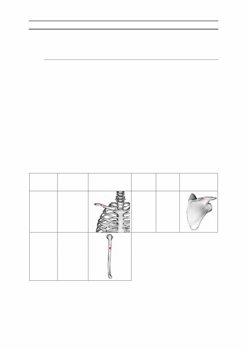
In-vivo intracortical experimentation
81
1. Validation data
1.1. Intracortical pins
The aim of this paragraph is to describe the protocol used by the S2M lab during their in vivo intracortical pins experiments.
In order to obtain validation data, motion captures were performed with the use of intracortical pins drilled in the bony segments (Dal Maso et al. 2014). As this method of validation is highly invasive, the protocol was thus only performed on two male volunteers (27/44 years old, 57/82 kg, 1.65/1.72 m) who signed an informed consent prior to the study. Both subjects obtained a score at the Disabilities of the Arm, Shoulder and Hand questionnaire (DASH) (Hudak et al., 1996) lower than 10.5, indicating no history of shoulder dysfunction, pain or injury. An experienced surgeon performed a local anaesthesia (AstraZeneca, Södertälje, Sweden) and inserted three self-drilling intracortical pins (Synthes, Bettlach, Switzerland) under normal and sterile surgery conditions. Pins (2.5mm of diameter) were positioned distal to the medial attachment of the deltoid on the humerus, on the scapula spine and on the superior part of the anterior concavity of the clavicle (Table 6).
Table 6 : Drill points positioning on the different body segments
Body Segment
Position Drill Point (indicated by red star)
Body Segment
Position Drill Point (indicated by red
star)
Clavicle
Superior part of the anterior concavity of the clavicle
Scapula Scapula spine
Humerus Medial
attachment of the deltoid
The position of the drill points were chosen to avoid any nerve, blood vessel and muscle, and not to have any modification in the muscle control strategy used by the subject during the movement. In addition, the intracortical pins position allowed the movements without any contact with the head or the neck of the subject. Clusters of 4 (scapula, clavicle) or 5 (humerus) markers were

In-vivo intracortical experimentation
82
finally connected firmly to the intracortical pins. After that, the rigidity of the montage was checked, insertion sites were sterilised and covered with sterile dressing. Pins were removed after the experiment and insertion sites were sterilised and covered again with new sterile dressing. The subjects were given pain relief (AstraZeneca, Södertälje, Sweden) and antibiotic to avoid any infection. Following the experiment, no clinical complication occurred for the subjects. Because STA were assumed to be small on the thorax compared to the distance between the markers, and because the intracortical pins fixation is difficult in the sternum, cutaneous markers were used on this segment. These markers were positioned on T1, T10, incisura jugularis (IJ) and processus xiphoid (PX) and completed by the set of 28 technical markers used by Jackson et al. (2012) on the whole upper limb (Figure 58 and Table 7).
All movements were recorded using a system of 18 optoelectronic VICONTM cameras (Oxford Metrics Ltd., Oxford, UK) at 100Hz. In order to follow ISB recommendations (Wu et al., 2005) for axes sequences and kinematics calculation, all ISB landmarks were pointed during a static record. The subjects then performed two repetitions of the three following tasks: abduction-adduction, flexion-extension, and internal-external rotation movements with a thoracohumeral abduction of 90° with the elbow flexed at 90°. These movements and the GH functional movements were used for the comparison of the MBO models. Optimisation and data processing were performed with Matlab after having imported the c3d files using the Biomechanical ToolKit (BTK) (Barre and Armand, 2014). For several movements, acquisition was split in two different trials (abduction-adduction and flexion-extension). For an ease of reading, as they were representative of the two trials, only the first is presented in the result part. The second can be found in the Appendix 2.
Figure 58: Landmarks and intracortical pins used in the experiment
(cutaneous markers with a red cross are not used in our study)

In-vivo intracortical experimentation
83
Table 7 : Markers abbreviation
Segment Abbreviation Name
Thorax
IJ Incisura jugularis IJp Projection of the incisura jugularis on the spine PX Processus Xiphoid PXp Projection of the processus Xiphoid on the back
Scapula Set Jackson et al.
AT Acromial Tip AA Angulus Acromialis SI Lateral point of the scapula spine Sm Medial point of the scapula spine
Scapula Set ISB
AT Acromial Tip AA Angulus acromialis TS Trigonum spinae AI Angulus Inferior
Humerus
Dlt Insertion of the deltoid Hl Humerus lateral Hm Humerus medial Hpu Humerus posterior up Hpd Humerus posterior down EM Medial Epicondyle
The experimental protocol was approved by the concerned local ethic committees of the Institut Karolinska (Sweden) and the University of Montréal (Canada).
1.2. Comparison method
For all the different studies of this chapter, similarly as in chapter 3, the accuracy of the different MBO models has been compared using the error between the kinematics obtained with the intracortical pins, which was considered as the reference, and the one obtained with applied MBO. These results were then plotted on boxplots and completed with RMSE and R2 as goodness-of-fit indicators (Figure 59). This comparison was performed for the three scapulothoracic Degrees of Freedom (DoF) (i.e., upward-downward rotation, protraction-retraction, and anterior-posterior tilt as defined by the ISB). The correlation levels were defined as follows: 0≤R2<0.3 was defined as a low correlation, 0.3≤R2<0.6 a medium correlation, 0.6≤R2<0.9 a high correlation and 0.9≤R2 a very high correlation.

In-vivo intracortical experimentation
84
Figure 59 : Box plot definition
2. Study 1: Ability of the different MBO models to mimic the bones kinematics
The aim of this study was to evaluate the ability of the different MBO models to mimic the bones kinematics similarly as the cadaveric study presented in Chapter 3.
2.1. Methods
The same MBO framework that was used for the cadaveric experiment (Chapter 3) was used for the optimisation except that the forearm model was not integrated. Thus, only the joint constraints of the shoulder complex were applied. The different geometric parameters were all defined thanks to functional methods using the intracortical pins. SC and AC centres – which define the clavicle constraint – were determined respectively by two functional movements: one maximising the movement of the clavicle relative to the thorax and one maximising the movement of the scapula relative to the clavicle. The functional movement used for the GH joint definition was composed of 3 flexions-extensions, 3 flexions in the scapular plane, 3 abduction-adduction and 6 circumductions. The SCoRE method (Ehrig et al., 2006) was then used to define GH, AC and SC joint centres. The thorax ellipsoid was also defined using a functional method. Its position was based on an ellipsoid fitting the trajectories of five markers positioned on the scapula (i.e., AA, TS, AI, Sl and Sm) during the 3 functional movements used for GH, AC and SC. The ellipsoid best minimising the distance between the ellipsoid surface and the different points trajectories was considered as the functional ellipsoid.
The same four scapulothoracic models that were studied based on the cadaveric experiment (Chapter 3) were compared here. Two models were defined by one contact point between this ellipsoid and the scapula defined as the midpoint between TS and AI (i.e., ST1a model) or as the centroid of TS, AI and AA (i.e., ST1b model), both projected on the ellipsoid during the static acquisition. Another model was defined with two contact points being TS and AI (i.e., ST2) as recommended by Garner and Pandy (1999). The last model constrained the scapula plane to be tangent to the ellipsoid (i.e., STT).

In-vivo intracortical experimentation
85
The ability of the different models to mimic the bones kinematics was then evaluated by using the different intracortical clusters as motor constraints (except for the thorax for which skin markers were used).
2.2. Results
The following paragraphs are related to the results obtained using intracortical clusters as motor constraints on the different scapulothoracic joint models (Figures 60 to 63).
Globally, the choice of the scapulothoracic joint model did not seem to impact importantly the results obtained. The subject 1 had a more mobile scapula since the range of motion for each DoF was always greater for all movements except for anterior-posterior tilt during the GH functional movements.
Figure 60 : Boxplots of the error existing between the bones kinematics and the different models kinematics using the intracortical pins as motor constraints for the anterior-posterior tilt, the upward-
downward rotation and the protraction-retraction during an abduction movement

In-vivo intracortical experimentation
86
Figure 61 : Boxplots of the error existing between the bones kinematics and the different models kinematics using the intracortical pins as motor constraints for the anterior-posterior tilt, the upward-
downward rotation and the protraction-retraction during a flexion movement.
Figure 62 : Boxplots of the error existing between the bones kinematics and the different models kinematics using the intracortical pins as motor constraints for the anterior-posterior tilt, the upward-
downward rotation and the protraction- retraction during the glenohumeral functional movement.
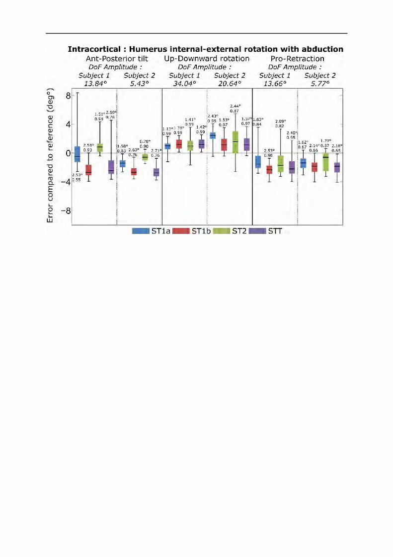
In-vivo intracortical experimentation
87
Figure 63 : Boxplots of the error existing between the bones kinematics and the different models kinematics using the intracortical pins as motor constraints for the anterior-posterior tilt, the upward-
downward rotation and the protraction-retraction during humerus internal-external rotation with abduction
2.2.1. Anterior-posterior tilt No marked difference was observed between the different models for anterior-posterior tilt except for movements implying abduction (i.e, abduction movement and humerus rotation with abduction). In those specific cases, ST1b and STT models presented greater RMSE. Similar ranges of error were found for subjects 1 and 2. During flexion movements, it was ST1a model that presents the highest range of error. The range of error was [-6.2°-8.4°] with a maximum RMSE of 3.94° for subject 1 and [-4.5°-5.8°] with a maximum RMSE of 2.89° for subject 2. The correlation between the MBO and bones kinematics was always high to very high except for specific cases generally associated with low anterior-posterior tilt amplitude.
2.2.2. Protraction-retraction Similarly to the anterior-posterior tilt, higher RMSE for ST1b and STT models were observed for protraction-retraction but only for pure abduction movements. The kinematics obtained with MBO presented generally a high to very high correlation with the bones kinematics. For some cases associated with low range of motion, the correlation could be low to medium. The errors obtained for both subjects were similar. The range of error was [-8.75° 3.58°] with a maximum RMSE of 4.39° for subject 1 and [-7.36° 1.64°] with a maximum RMSE of 3.32° for subject 2.

In-vivo intracortical experimentation
88
2.2.3. Upward-downward rotation No marked difference could be observed between the different models for upward-downward rotation. The correlation was always very high for all movements, subjects and constraint models. The use of MBO tended to slightly overestimate the upward-downward rotation for both subjects. The error obtained was greater for subject 2 but stayed relatively low compared to the upward-downward rotation amplitude [20.64° 43.77°]. The range of error was [-3.24° 3.58°] for subject 1 with a maximum RMSE of 2.20° and [-2.59° 6.77°] with a maximum RMSE of 4.40° for subject 2. ST2 seemed obtaining higher range of error than the other models on specific movements (i.e., GH functional movements and humerus internal-external rotation with abduction) for both subjects.
2.3. Discussion
Concerning the ability of the model to mimic bones kinematics, the results found in this in vivo intracortical pins study were similar to the ones obtained with the cadaveric studies (Chapter 3). Indeed, no important difference could be found between the different scapulothoracic models. Except for specific movements containing abduction, the results obtained for the different models were relatively similar. The remaining difference might be due to a poor definition of the ellipsoid. It has been shown in Chapter 3 that this ellipsoid might modify the ability of the different scapulothoracic kinematic models to mimic the bones kinematics. Consequently, the same conclusion could be used here. As a result, even if the different models were equally able to mimic the bones kinematics, the model tangent to an ellipsoid should be preferred since it should allow a more precise calculation for kinetics and further musculoskeletal development (cf Chapter 3).
3. Study 2: Ability of the different MBO models to correct Soft Tissue Artefact
As the ability of the different scapulothoracic joint kinematic models to mimic the bones kinematics has been evaluated in both a cadaveric and in vivo intracortical pins studies, it is now necessary to evaluate the ability of these models to correct STA-related errors.
3.1. Method
The same scapulothoracic joint models than for study 1 were compared here, except that the geometry of the models was obtained using the functional methods on the landmarks instead of the intracortical pins. This was done in order to replicate the results that could be obtained during daily clinical experiments where the intracortical pins would not be available for the definition of the model for evident ethical reasons.
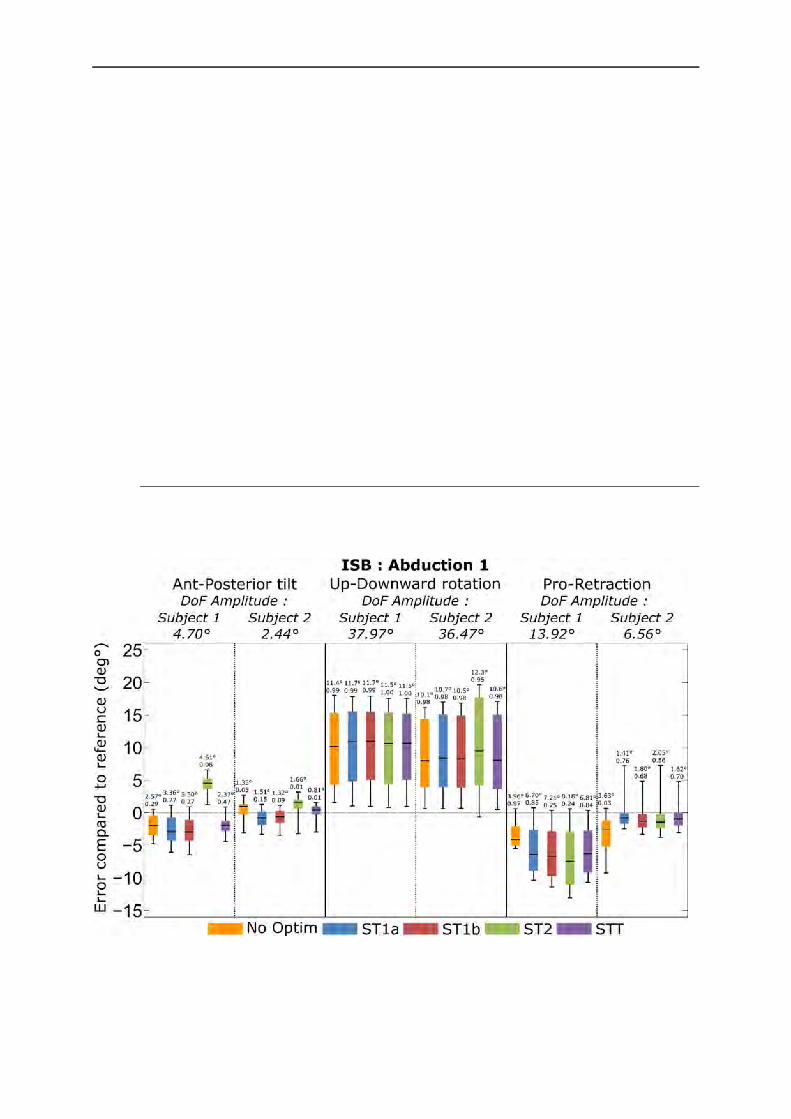
In-vivo intracortical experimentation
89
The ability of the models to correct the STA-related errors has been evaluated by using the cutaneous landmarks as motor constraints. As two sets of markers (i.e., ISB (Wu et al., 2005) and Jackson et al. (2012)) were available for the scapula and may induce different motor constraints (Lu and O’Connor, 1999; Roux et al., 2002), both were used in separated assessments to be compared. Then, it was assumed that understanding the effects of the different motor constraints on our models would allow a better definition of them. In order to assess the models ability to correct STA-related errors, a kinematic calculation without MBO (No-optim) was also performed. This was achieved by using the same optimisation procedure without any joint kinematic constraint. Consequently, the position of the different body segments was determined only by the motor and rigid constraints. The resulting position of each segment corresponds then to the position for which the associated cluster of cutaneous markers is less deformed (i.e., minimisation of the distance between the measured markers and the rigid cluster defined in static position). It then corresponds to a CAST method (Chiari et al., 2005) where the cluster shape was defined as the relative mean position of each constituting landmark during a static acquisition.
3.2. Results: using ISB motor constraints
The following paragraphs are related to the results obtained using ISB motor constraints on the different scapulothoracic joint kinematic models. (Figures 64 to 67)
Figure 64 : Boxplots of the error existing between the bones kinematics and the different models kinematics using the ISB marker set as motor constraints for the anterior-posterior tilt, the upward-
downward rotation and the protraction-retraction during an abduction movement

In-vivo intracortical experimentation
90
Figure 65 : Boxplots of the error existing between the bones kinematics and the different models kinematics using the ISB marker set as motor constraints for the anterior-posterior tilt, the upward-
downward rotation and the protraction-retraction during a flexion movement
Figure 66 : Boxplots of the error existing between the bones kinematics and the different models kinematics using the ISB marker set as motor constraints for the anterior-posterior tilt, the upward-
downward rotation and the protraction-retraction during the glenohumeral functional movement

In-vivo intracortical experimentation
91
Figure 67 : Boxplots of the error existing between the bones kinematics and the different models kinematics using the ISB marker set as motor constraints for the anterior-posterior tilt, the upward-downward rotation and the protraction-retraction during humerus internal-external rotation with
abduction
3.2.1. Upward-downward rotation No important difference in RMSE and range of error could be observed between the different models and the one not using any kinematic constraint when considering upward-downward rotation. The kinematics obtained was always highly correlated with the bones kinematics. The errors on subject 2 were lower than those of subject 1 but were also associated with lower movements’ amplitude. The range of error was [-0.25° 22.80°] for subject 1 with a maximum RMSE of 14.63° and [-0.63° 19.65°] with a maximum RMSE of 12.65° for subject 2. When no kinematic constraint was used, the range of error was [0.02° 21.88°] with a maximum RMSE of 13.60° for subject 1 and [-0.23° 16.20°] with a maximum RMSE of 11.06° for subject 2.
3.2.2. Protraction-retraction When considering protraction-retraction, no difference in RMSE and range of error could be observed between the different models. The correlation was always high to very high for all movements and models for both subjects when MBO was used, except for some specific cases associated with lower amplitude of protraction-retraction. In that later case, correlation from low to medium could be found. For subject 1, errors tended to be greater when MBO was used whereas the opposite result was observed for subject 2. The range of error was [-15.38° 1.22°] for subject 1 with a maximum RMSE of 8.62° and [-6.41° 7.29°] with a maximum RMSE of 12.65°

In-vivo intracortical experimentation
92
for subject 2. When no kinematic constraint was used the range of error was [-9.71 0.88] with a maximum RMSE 4.47° for subject 1 and [-9.27° 1.06°] with a maximum RMSE of 4.07°.
3.2.3. Anterior-posterior tilt No important difference could be observed between the different joint kinematic models except for the ST2 model when considering the anterior-posterior tilt. The range of error obtained with ST1a, ST1b and STT tended to be similar to the one without kinematic constraint. With or without kinematic constraint, the correlation tended to be low to medium. The range of error was [-6.59° 13.10°] with a maximum RMSE of 6.28° for subject 1, and a range of error of [-5.05° 6.62°] with a maximum RMSE of 3.56° was observed for subject 2. When the ST2 model was not considered, the range of error was [-6.59 5.93] with a maximum RMSE of 3.50° for subject 1, and [-5.05° 6.07°] with a maximum RMSE 2.84 ° for subject 2. When no kinematic constraint was used, the range of error was [-5.75° 3.21°] with a maximum RMSE of 2.90° for subject 1 and [-9.38° 7.19°] with a maximum RMSE of 3.88° for subject 2.
3.3. Results: using Jackson et al. motor constraints
The following paragraphs are related to the results obtained using Jackson et al. motor constraints on the different scapulothoracic joint kinematic models (Figures 68 to 71).
3.3.1. Upward-downward rotation The error using MBO tended to be higher or equivalent to the one without correction for upward-downward rotation. The correlation between the bones kinematics and the one obtained with MBO was always very high. The range of error was [-3.34° 8.46°] for subject 1 with a maximum RMSE of 4.64° and [-2.69° 6.24°] with a maximum RMSE of 3.34° for subject 2. When no kinematic constraint was used, the range of error was [-3.44° 15.65°] with a maximum RMSE of 4.46° for subject 1 and [-3.30° 4.39°] with a maximum RMSE of 1.93° for subject 2.
3.3.2. Protraction-retraction The use of MBO tended to increase importantly the error obtained with the protraction-retraction for the subject 2, except for the humerus internal-external rotation with abduction and GH functional movements. The protraction-retraction error obtained with and without kinematic constraint was similar for the subject 1. The correlation obtained was always high to very high. The range of error was [-7.90° 3.91°] for subject 1 with a maximum RMSE of 3.19° and [-1.46° 7.90°] with a maximum RMSE of 7.90° for subject 2. When no kinematic constraint was used, the range of error was [-7.27° 5.37°] with a maximum RMSE 3.52° for subject 1 and [-3.17° 11.06°] with a maximum RMSE of 2.25°.

In-vivo intracortical experimentation
93
3.3.3. Anterior-posterior tilt When considering anterior-posterior tilt, very high error, up to 80°, could be found if no correction was used. This was generally associated with the loss of the AT marker during the data collection. When no marker was lost, the errors were equivalent with and without kinematic constraints and no important difference was found between the different MBO models. The error found for the different MBO models seemed important considering the amplitude of anterior posterior tilt [2.41° 16.09°]. Indeed, the range of error was [-8.75° 12.05°] for subject 1 with a maximum RMSE of 5.09° and [-7.91° 4.12°] with a maximum RMSE of 2.36° for subject 2. When no kinematic constraint was used, the range of error was [-87.05° 7.14°] with a maximum RMSE 26.28° for subject 1 and [-30.54° 23.51°] with a maximum RMSE of 14.15° for subject 2.
Figure 68 : Boxplots of the error existing between the bones kinematics and the different models kinematics using the Jackson et al. marker set as motor constraints for the anterior-posterior tilt, the
upward-downward rotation and the protraction retraction during an abduction movement

In-vivo intracortical experimentation
94
Figure 69 : Boxplots of the error existing between the bones kinematics and the different models kinematics using the Jackson et al. marker set as motor constraints for the anterior-posterior tilt, the
upward-downward rotation and the protraction retraction during a flexion movement
Figure 70 : Boxplots of the error existing between the bones kinematics and the different models kinematics using the Jackson et al. marker set as motor constraints for the anterior-posterior tilt, the
upward-downward rotation and the protraction retraction during the glenohumeral functional movement

In-vivo intracortical experimentation
95
Figure 71 : Boxplots of the error existing between the bones kinematics and the different models kinematics using the Jackson et al. marker set as motor constraints for the anterior-posterior tilt, the
upward-downward rotation and the protraction retraction during the humerus internal-external rotation with abduction
3.4. Discussion
Concerning the ability of the model to correct STA-related errors, the results were mitigated. The choice of the joint kinematic model had a small influence on the level of correction obtained. Indeed, the results were far more influenced by the marker set than the kinematic constraints. Globally, the use of MBO seemed to have an impact mainly on the protraction-retraction and anterior-posterior tilt. However, the upward-downward was the scapula’s DoF the most affected by STA in term of amplitude (Matsui et al., 2006). Indeed, high errors were obtained in upward-downward rotation when the ISB marker set was used.
Considering the Jackson et al. marker set, marked errors have been observed when no correction was used. This was due to the loss of the AT marker during movements with high range of motion. In that case, the AT marker was likely to be hidden by the head/neck and/or the arm of the subject (in the Jackson et al. marker set, the AT marker was located on the anterior part of the scapula (AT) and three markers aligned on the scapula spine (AA Sl Sm)). When no kinematic constraint was used, the reconstruction was done only by minimising the distance between the reconstructed markers and the measured ones. Consequently, when the AT marker was lost, the reconstruction was done only on the 3 scapula spine aligned markers (i.e, AA, Sl, Sm). It results that the rotation of the reconstructed cluster around the scapula spine axis was free (Figure 72).

In-vivo intracortical experimentation
96
Figure 72 : Rotation of the scapula reconstructed SCS around the scapula spine axis when the AT marker is lost
This axis corresponded to the anterior-posterior tilt axis of rotation. It then explains the high errors obtained for this DoF. In those specific cases, the use of MBO allowed correcting importantly the error. Indeed, high anterior or posterior tilt were incompatible with the different scapulothoracic constraints used (i.e., point in contact or plan tangent to an ellipsoid). However, when no loss of marker was identified, the errors obtained with MBO were equivalent to the errors without correction. These errors due to the loss of one marker (AT) were not observed when the ISB marker set was used. Indeed, the ISB marker set integrates the use of the AI marker. This marker was less likely to be lost during movement, and then allowed a better definition of SCS in the anterior-posterior tilt DoF. Lower errors were then observed for the anterior-posterior tilt with the ISB marker set, but at the cost of far higher upward-downward rotation errors. This was due to the use of AI and TS for the motor constraints. Indeed, these two markers were more sensible to STA than the one near AA in this specific DoF (Matsui et al., 2006). However, in those cases, the upward-downward error was not corrected by the use of MBO as it was for the anterior-posterior tilt for the Jackson et al. marker set. The limitation of the different joint kinematic models used in MBO for correcting the upward-downward rotation were then highlighted again.
Consequently, according to this result, the MBO had small impact on the upward-downward rotation and was able to correct the other DoFs only if they were highly unphysiological (e.g., loss of a marker determinant for the anterior-posterior tilt). As suggested in the Chapter 3, the rotation around the upward-downward rotation axis was less constrained than the other DoFs with the different joint kinematic models. Indeed, these models impacted mainly the direction of the vector normal to the ellipsoid which was the upward-downward rotation axis.
4. Study 3: Simpler STA correction method MultiBody Optimisation (MBO) is a complex method implying long computation time and reliant on an important number of geometrical construction parameters that can be difficult to personalise. As shown in study 2, MBO did not allow correcting in a marked manner the Soft Tissue Artefact (STA). Only highly unphysiological kinematics, due to markers loss, was

In-vivo intracortical experimentation
97
corrected. When degrees of freedom (DoF) with small amplitude were considered, the results were very unsatisfying knowing the computation time and the complexity of the method involved. Consequently, considering the small benefice obtained, MBO did not seem viable in a clinical context for correcting STA-related errors. The initial aim of this thesis was to propose a method allowing to correct STA-related errors in a clinical context, which was thus not currently fulfilled. Nevertheless, in study 2, interesting results arose from the comparison between the ISB and Jackson et al. marker sets. Indeed, it has been observed that each marker set was giving access to accurate results for different DoF. The ISB marker set avoided the errors due to the AT marker loss in anterior-posterior tilt observed when the Jackson et al. marker set was used. Inversely, the Jackson et al. marker set allowed obtaining lower errors than the ISB marker set when considering the upward-downward rotation. Consequently, it seemed that accurate information were held in each markers set but were perturbed for specific DoFs. It would thus be interesting to investigate if there is a method that would allow to extract these informations, combining the different marker sets in order to obtain less STA-related error based only on the markers position instead of using complex MBO models. One first solution could then be to build the scapula SCS using a different set of markers. The next study then aimed to:
- Develop and present such a method involving less parameters than MBO and based exclusively on markers position
- Evaluate the capacity of this method to correct STA-related errors based on intracortical pins experiment data (see study 2)
4.1. The neglected-Degree of Freedom method
4.1.1. Equation Initially, the neglected-Degree of Freedom (n-DoF) method has been developed to solve the problem of the loss of the AT marker. Indeed, during some acquisitions, the loss of this marker resulted in wrong kinematics as the other markers were aligned along the scapula spine. Consequently, the scapula was free to rotate around this axis which corresponds to the anterior-posterior tilt axis. As a result, important errors were found for this specific DoF. It was first tested to use directly AI landmark as it is unlikely to be hidden during acquisition. However, this resulted in a high error in upward-downward rotation as large STA are generally associated with this marker on this specific DoF. Consequently, the idea of using this marker and neglecting its impact on the upward-downward rotation arose.
In order to eliminate the influence of a marker on one specific degree of rotation, we projected this point on the corresponding axis of rotation. Consequently, the difference between the
measured marker jiMr and the modelled marker j
iMi iN Q has to be projected on the axis of rotation
jii inN Q . As a result, the initial motor constraint that was 3 1
ji
ji
Mi iM r N Q 0 became:

In-vivo intracortical experimentation
98
3 1( )j ji i
ji
Mi i i iM nNr N Q Q 0 4.1
With the associated Jacobian:
( ) * ( ) *j j j ji i i i
ji
M MTi i i i i iM
mij n nQ N r N QK N N 4.2
These two new equations could be used directly in the cost function constraint formula:
Φ Φ1
2
Tm mf 4.3
With the associated Jacobian formula:
Φ*Tf m m
K K 4.4
The markers that were fully used are now called jiMr and the ones on which the rotation was
neglected jiM rotr .
4.1.2. Experimentation: definition of different marker sets
The evaluation of the new method was performed using the intracortical experimental protocol on the same subjects and set of movements than the different MBO models.
The n-DoF method was compared to the use of the classical marker set proposed by ISB (Wu et al., 2005) and Jackson et al. (Jackson et al., 2012). Four marker sets were then tested (Figure 73). In addition to the two marker sets that were used in the chapter 4 (i.e, Jackson et al. and ISB), the Jackson et al. marker set was completed with the marker AI with its effect on the upward-downward rotation axis (i.e., normal to the scapula plane) neglected (rMrotAI). Finally, for the last marker set, the AT marker was completely removed conserving the AI marker with its effect on the upward-downward rotation axis neglected (rMrotAInoAT).
Figure 73 : The different marker sets evaluated

In-vivo intracortical experimentation
99
4.2. Results
The following paragraphs are related to the results comparing the different marker sets integrating the n-DoF method to the ISB and Jackson et al. marker sets (Figures 74 to 77).
4.2.1. Anterior-posterior tilt For the anterior-posterior tilt, the ISB marker set allowed obtaining better results than the Jackson et al. marker set. Indeed, when the Jackson et al. marker set was considered, the range of error was [-87.05° 7.14°] with a maximum RMSE 26.28° for subject 1 and [-30.54° 23.51°] with a maximum RMSE of 14.15° for subject 2. The error decreased importantly when considering the ISB marker set. In that case, the range of error was [-5.75 3.21] with a maximum RMSE of 2.90° for subject 1 and [-9.38° 7.19°] with a maximum RMSE of 3.88° for subject 2.
No important difference can be observed between rMrotAI and rMrotAInoAT. The error levels were similar to the ones found when ISB marker set is used. Indeed, when considering both rMrotAI and rMrotAInoAT, the range of error was [-6.58° 4.46°] with a maximum RMSE 3.33° for subject 1 and [-7.91° 4.12°] with a maximum RMSE of 2.38° for subject 2. The correlation for the different marker sets could be low for movements involving a low anterior-posterior amplitude but tended to be generally medium to high.
4.2.2. Upward-downward rotation When the Jackson et al. marker set was used, the range of error is [-3.44° 15.65°] with a maximum RMSE of 4.46° for subject 1 and [-3.30° 4.39°] with a maximum RMSE of 1.93° for subject 2. In contrast to anterior-posterior tilt, errors obtained with the ISB marker set were higher for this DoF. Indeed, when the ISB marker set was used, the range of error was [0.02° 21.88°] with a maximum RMSE of 13.60° for subject 1 and [-0.23° 16.20°] with a maximum RMSE of 11.06° for subject 2.
For the upward-downward rotation, rMrotAI and rMrotAInoAT gave results with a similar range of error than the Jackson et al. marker set. The rMrotAInoAT seemed to furnish better results for this DoF than rMrotAI. Indeed, when considering rMrotAI, the range of error was [-4.48° 4.78°] with a maximum RMSE of 2.33° for subject 1 and [-5.11° 1.52°] with a maximum RMSE of 1.53° for subject 2. The error level dropped slightly when rMrotAInoAT was considered. Indeed, in that case, the range of error was [-3.36° 1.79°] with a maximum RMSE of 1.29° for subject 1 and [-2.6° 1.80°] with a maximum RMSE of 1.17° for subject 2. For this DoF, the rMrotAI and rMrotAINoAT correlation with the reference was always very high and always equivalent to the correlation obtained with the Jackson et al. and ISB marker sets.
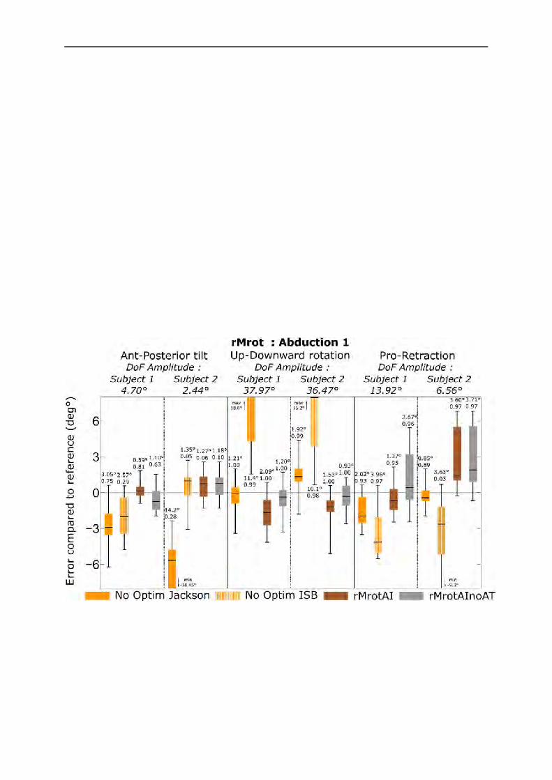
In-vivo intracortical experimentation
100
4.2.3. Protraction-retraction For protraction-retraction, the two marker sets were almost equivalent, the Jackson et al. marker set having a slightly lower error than the ISB marker set. Indeed, when the ISB marker set was used, the range of error was [-9.71° 0.88°] with a maximum RMSE 4.47° for subject 1 and a range of error of [-9.27° 1.06°] with a maximum RMSE of 4.07°. For the Jackson et al. marker set, the range of error was [-7.27° 5.37°] with a maximum RMSE 3.52° for subject 1 and [-3.17° 11.06°] with a maximum RMSE of 2.25°.
No important difference was observed between rMrotAI and rMrotAInoAT when considering the protraction-retraction DoF and the errors were similar than those observed using the Jackson et al. marker set. When considering both rMrotAI and rMrotAInoAT, the range of error was [-3.59° 6.94°] with a maximum RMSE 2.86° for subject 1 and [-2.31° 6.80°] with a maximum RMSE of 3.71° for subject 2. For this DoF, the rMrotAI and rMrotAInoAT correlation with the reference was always high to very high and always above the correlation level obtained with the Jackson et al. or ISB marker sets.
Figure 74 : Boxplots of the error existing between the bones kinematics and that obtained using different marker sets for the anterior-posterior tilt, the upward-downward rotation and the protraction-retraction
during an abduction movement
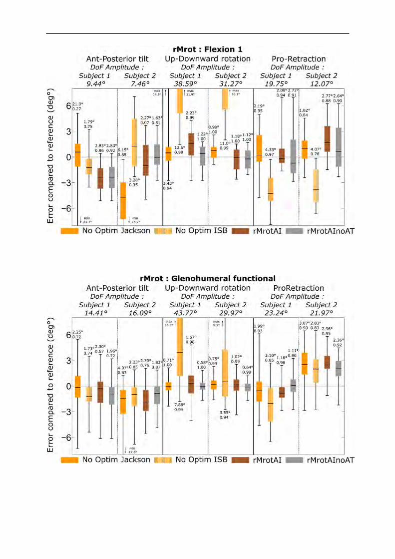
In-vivo intracortical experimentation
101
Figure 75 : Boxplots of the error existing between the bones kinematics and that obtained using different marker sets for the anterior-posterior tilt, the upward-downward rotation and the protraction-retraction
during a flexion movement
Figure 76 : Boxplots of the error existing between the bones kinematics and that obtained using different marker sets for the anterior-posterior tilt, the upward-downward rotation and the protraction-retraction
during the glenohumeral functional movement

In-vivo intracortical experimentation
102
Figure 77 : Boxplots of the error existing between the bones kinematics and that obtained using different marker sets for the anterior-posterior tilt, the upward-downward rotation and the protraction-
retraction during the humerus internal-external rotation with abduction
4.3. Discussion
On one hand, the use of the ISB marker set allowed avoiding markers loss problem during the acquisition, associated with higher errors on upward-downward rotation. In the other hand, the Jackson et al. marker set allowed lower errors on this DoF, but was more prone to markers losses for movements with high amplitude (mainly on AT marker).
As expected, the use of the n-DoF method allowed neglecting the effect of a marker on a specific axis of rotation. Indeed, as shown, when this method was used, it was possible to correct the error on the anterior-posterior tilt without increasing the error on the upward-downward rotation. This was not the case when the Jackson et al. marker set was replaced by the ISB marker set. It was thus possible to combine the accurate information of each marker set in the building of a single SCS.
The errors obtained when the n-DoF method was used are always equivalent or lower than when the classical marker sets were used, giving the best results for each DoF even if less satisfying for protraction-retraction DoF. As only one SCS should be defined in order to allow kinematics computation, the use of the n-DoF method combined to the Jackson et al. marker set (with and without AT marker) seemed allowing the global best results in all DoF. When the MBO models were used in the previous chapter, for some specific cases, lower error than with the n-DoF method were found. However, the result obtained with the n-DoF method seemed more consistent

In-vivo intracortical experimentation
103
than MBO. As an example, for the protraction-retraction DoF, the Jackson et al. marker set led to a low error for subject 1 but a high error for subject 2 when similar error levels were observed without corrections for both subject. The opposite phenomenon was observed when the ISB markers were used as motor constraints. Consequently, the comparison between these two subjects using MBO as a method for correcting STA-related errors could be erroneous. With the n-DoF method, the error level seemed similar regardless of the movement or the subject. As repeatability of data seem more important than trueness for comparison in a clinical context, the n-DoF method should then be preferred for its consistency.
In addition, the n-DoF method was directly based on markers position, making it adapted to each patient without any need for specific measurement or definition of geometric parameters adapted to their morphology. This method could then be used a posteriori. Indeed, generally, movement analysis laboratories had already performed an important number of data acquisitions with a specific marker set and constituted important database available for their research and medical activities. A change of marker sets could result in a protocol rupture and then a loss or incompatibility of data. In order to keep the same marker set, a posteriori methods for correcting STA-related error should be interesting. The n-DoF method could be used a posteriori and does not need any change in the marker set or new movement acquisitions as the neglected markers can be changed easily. MBO, in a certain way, can also be used a posteriori. However, the tuning of the geometric parameters can be difficult and may need specific functional movements data collect. Consequently, MBO, used as an a posteriori method, could be more difficult to apply than the n-DoF method.
In the end, this n-DoF method can also be associated with a MBO model as the fact of neglecting the impact of a marker relative to an axis may be defined as a motor constraint. It should then allow increasing the quality of the motor constraints used in MBO and thus improve the method precision. Consequently, the n-DoF method seems both adapted for a direct use in a clinical context and for further development of MBO models in a musculoskeletal approach.
5. Limits These studies, similarly to the cadaveric studies (see Chapter 3), were strongly limited by the number of subjects. Indeed, as the use of intracortical pins was very invasive, it was difficult to conduct the experiment on more than two subjects. However, the small sample of subjects was equivalent to similar studies based on intracortical pins (Arndt et al., 2004; Braman et al., 2010; Houck et al., 2015).
In addition, the geometry construction parameters, needed for MBO, remained a problem as all these parameters have been determined using functional methods. The quality of these methods should be investigated with a particular attention on the ellipsoid modelling the thorax. Indeed, as it has been seen in Chapter 3, the ellipsoid parameters used can change the results obtained in term of ability to mimic the bones kinematics.

In-vivo intracortical experimentation
104
The error obtained without correction for the Jackson et al. marker set in upward-downward rotation, with MBO or with the n-DoF method, is low and thus suspicious. It could be understand that the error was lower than the one obtained with the ISB marker set. Indeed, as the AI marker is known for being more impacted by STA than the markers close to the AA marker (Matsui et al., 2006), its use should result in an important error in the upward-downward rotation. However, obtaining such a small error seemed suspicious as, even with markers positioned on the scapula spine, higher errors were expected. However, it should be noted that the AA, Sl and Sm markers were located close to an intracortical pin which has been covered with sterile dressing maintained with tape (Figure 78).
Figure 78 : Intracortical pins and tape positioning near the scapula for Jackson et al. marker set
It meant that this skin in the area may have been affected, due to the tape, by the movement of the intracortical pin and thus that STA-related errors may have been reduced. As the upward-downward rotation is directly linked to the displacements of these 3 markers (i.e., AA, Sl, Sm markers), it might result that the error obtained on upward-downward rotation was reduced. The aim of the study 3 was to prove that the n-DoF method allowed effectively neglecting a specific DoF for a specific marker and the MBO method has been shown not to impact the upward-downward rotation. Consequently, this limitation does not impact the findings of the studies 2 and 3. However, it must be considered that higher upward-downward STA-related errors might be found when the Jackson et al. marker set is combined with the n-DoF or MBO methods without the intracortical pins and the tape maintaining the sterile dressing.
In the end, the use of intracortical pins might have also perturbed the scapula kinematics due to discomfort or pain of the subject. This seems more likely for subject 2 as its scapula range of motion was generally lower than that of subject 1.
6. Conclusion Similarly to the cadaveric studies, the different scapulothoracic models seemed equally able to mimic the bones kinematics obtained with in vivo intracortical pins experiments data. However, the STA-related errors correction obtained using MBO could be disappointing. Indeed, except for highly unphysiological errors, the correction obtained was not that marked. Consequently, the use of MBO for correcting STA-related errors in a clinical context seemed compromised.

In-vivo intracortical experimentation
105
Firstly, this method is complex and implies a non negligible computation time (i.e., around 0.3-0.5 sec per frame). In addition, the results can be dependent on an important number of geometrical construction parameters that can be difficult to obtain. The use of imaging technics allows a good definition of these parameters but, in a daily routine, it could be difficult and harmful for the patient due to radiation. Consequently, there remains a need for improving the correction of STA-related errors and to define a method that could be used in a simply manner during clinical routines. The use of the n-DoF method allowed to partially solve this problem. The aim of this method was to correct the anterior-posterior tilt introduced by the loss of the AT marker in the Jackson et al. marker set without introducing the high errors obtained in the ISB marker set in upward-downward rotation. The n-DoF method, used on the AI marker relative to the normal to the scapula plane, combined to the Jackson et al marker set, corrected this error. The n-DoF method allowed thus neglecting the effect of a specific marker around a defined DoF. This method was exclusively based on markers position which make it simpler than the MBO as less parameters are involved in its definition. In addition, the n-DoF method allowed also reducing effectively the STA-related errors. As a result, this method seemed well adapted for reducing STA-related errors in a clinical context. The next step would be to define, for each DoF, the markers that should be ignored in order to design the best marker set adapted for the scapula. As this method can be used on any markers and any axis, this approach should thus be adapted and extended to each measured body segment.

106
General conclusion
1. Thesis outcomes
1.1. MultiBody Optimisation as a tool for correcting Soft Tissue Artefact
The initial aim of this thesis was to develop a method allowing to correct Soft Tissue Artefact (STA)related errors in a clinical context. As it was shown in Chapter 1, the MultiBody Optimisation (MBO) approach has been chosen for multiple reasons. Firstly, MBO is based on the movements and morphology of each subject which is not the case with regression methods. Indeed, a personalisation of each joint kinematic model and geometry can be done using MBO whereas regression methods can only be used on the population they were defined on. Secondly, MBO can be used for complex movements investigation contrary to double calibration methods which are adapted only for one Degree of Freedom (DoF) movements. Thirdly, MBO avoids the segments dislocation that can be found when using simple optimisation methods which are based on the minimisation of the deformation of a cluster of markers. Finally, MBO has already been experienced and validated on the lower limb with promising results. In addition, this thesis was a first step toward the development of an upper limb musculoskeletal model, through the definition of reliable kinematic models.
1.2. Kinematic chain model development
A more physiological kinematic chain of the upper limb has been developed. This chain was based on more realistic constraints, defined through joint kinematic models, that were expected to allow obtaining better results similarly as for the lower limb. For example, the shoulder girdle was then not considered as a simple glenohumeral joint, but as a complex considering the thorax, the clavicle, the scapula and the humerus (i.e., the full shoulder complex). In addition, the shoulder complex was defined as a closed loop mechanism considering the scapulothoracic joint in addition to the sternoclavicular, acromioclavicular and glenohumeral joints. A new physiological definition of the scapulothoracic joint was also integrated. The associated constraint allowed positioning the scapula plane tangent to an ellipsoid modelling the thorax. This model was compared to existing joint kinematic models based on constraint points in contact with the thorax ellipsoid. In addition, the forearm was modelled as a closed loop integrating the behaviour of the radius and the ulna and based on the existing model of Pennestri et al. (2007). This later model was compared with a common model based on a universal joint between the humerus and the forearm.

General conclusion
107
1.3. Models validation: Intracortical pins
As data obtained through the use of intracortical pins are generally considered as a gold standard for kinematics, our model was confronted to two experiments based on this technic: a cadaveric study and an in vivo study. The ability of the different joint kinematic models to mimic the bones kinematics and to correct STA-related errors was evaluated. The forearm joint kinematic models were only assessed using the cadaveric study records whereas the scapulothoracic joint kinematic models were also evaluated using the in vivo study records. In addition to joint kinematic validation, the cadaveric study allowed investigating the effect of two different geometries on the model outcomes. Indeed, a CT-scan acquisition was performed on the frozen cadaver in the anatomical position and compared with the geometry obtained by scaling the model on the geometry provided by the Visible Human Project dataset.
Concerning the ability of the new joint kinematic models (i.e., tangent to an ellipsoid for the scapulothoracic joint and closed loop model for the forearm) to mimic the true upper limb kinematics, the results were similar to the former models. As suggested by the cadaveric study, it seems that the scapulothoracic joint kinematic model might be more sensible to the geometric parameters than the forearm model. However, these two new models allow obtaining additional information:
- The closed loop forearm joint kinematic model allows representing the existing movement between the ulna and the radius.
- The tangent to an ellipsoid scapulothoracic joint kinematic model allows a more physiological representation of the scapulothoracic joint with a moving constraint point.
Concerning the correction of STA-related errors, the use of MBO models does not seem well adapted. Indeed, the correction obtained was relevant only for highly unphysiological movements, while the results obtained for DoF with small amplitude were unsatisfying. As MBO is a complex method implying an important number of parameters that need to be personalised, its use in a clinical context seems compromised. As a result, it seems that MBO might not be the best solution for the correction of STA-related errors of upper limb in a clinical context. A simpler method was thus developed. This method, called n-DoF method (i.e., neglected degree of freedom), allowed neglecting the effect of a marker on a specific DoF. This method seems promising for the scapula, and could even be used with MBO or adapted to any other body segment.
1.4. Conclusion
Although the results were not as concluding as expected for the correction of STA-related errors, the joint kinematic models developed during this thesis may be relevant considering the development of a future upper limb musculoskeletal model. Indeed, for the forearm, it will be possible to integrate the different muscles connecting the ulna to the radius which would not

General conclusion
108
have been possible using the common universal joint model. Moreover, contrary to the former scapulothoracic joint kinematic models (i.e., based on constraint points), the tangent to an ellipsoid model allows the constraint point moving with respect to the scapula and to be equivalent to the contact point. As the position of this constraint point can change importantly the different muscular lever arms, obtaining a more realistic constraint point equivalent to the contact point should allow obtaining a more precise dynamic and musculoskeletal model.
Consequently, this thesis allowed building a complete anatomical upper limb kinematic chain expressed in natural coordinates for correcting STA through the use of a MBO framework. Although the correction of STA obtained was not as good as expected, the use of this approach for the development of a future musculoskeletal model has been validated.
2. Perspectives The different works proposed in this thesis might be completed by several studies in order to improve the proposed joint kinematic models:
Geometric parameters personalisation
The use of MBO implies using joint kinematic constraints associated to geometric parameters. As it has been shown during this thesis, these parameters can impact importantly the outcomes of the MBO. Consequently, in order to be able to use more anatomical models, personalisation possibility and precision should be investigated:
- Firstly, the use of simpler and less invasive imaging technics such as bi-planar low dose X-ray imaging system (e.g., EOS®) should be evaluated (Wybier and Bossard, 2013). Indeed, this technic is less ionising for the subject than traditional X-ray technics and should allow obtaining 3D geometric parameters. Its use for obtaining these personalised geometric parameters seems thus justified in a clinical context (McKenna et al., 2012).
- Secondly, as imaging technics are not available in all laboratories, the trueness and the precision of the different functional methods that have been presented and used in this thesis should be studied in more details. Indeed, the model personalisation through the use of functional methods seems currently the best compromise in a clinical context as it is completely harmless and allows obtaining geometrical construction parameters adapted to each subject (Ehrig et al., 2011, 2007).
- Last but not least, as some subjects might be unable to perform the movements needed for the different functional methods, scaling method should be preferred. Having a more detailed and precise generic model for scaling would then be useful. Indeed, it would allow obtaining a model geometry closer to the subject anatomy and then approaching a true personalised geometry. It could be done by extracting precisely all the geometrical

General conclusion
109
construction parameters that were obtained during our cadaveric study. It would combine both the 3D geometric parameters obtained with a CT-scan in the anatomical position and the ones obtained through the different functional methods that were performed during the motion capture acquisitions.
However, before being interested in the definition of a personalised model, the impact of the different geometrical construction parameters on the kinematics should be evaluated. Indeed, it would be useless to define precisely parameters that have no impact on the outcomes. Knowing the impact of each parameter would allow determining which parameter should be defined in priority in the personalisation procedure. This can be done through a sensivity analysis (Frey and Patil, 2002). A sensivity analysis gives the uncertainty on the outcomes of the model based on the uncertainty on the input used, in our case the geometric parameters (Ardestani et al., 2015; El Habachi et al., 2015b). Such a study would allow evaluating precisely the robustness of our model and having a correct understanding of the real error that could be expected using MBO.
New kinematic constraint models
New scapulothoracic joint kinematic models based on our tangent to an ellipsoid model could also be developed. Indeed, in this thesis the plane constrained to be tangent to the ellipsoid was automatically the plane defined by the vector scapu which was the scapula plane defined by the
AI TS AA markers (Figure 79).
Figure 79 : Scapulothoracic joint modelled as a plane tangent to an ellipsoid (left) and the different scapula and humerus bones landmarks (right)
Allowing to have a plane with a normal different from scapu could allow defining a further variety
of models. For example, a plane could be defined in a similar manner than the constraint point used in the scapulothoracic joint kinematic models. A point would thus be chosen on the scapula and projected on the ellipsoid according to the normal to the scapula plane. The tangent plane

General conclusion
110
at this point on the thorax ellipsoid would be defined as the plane that should be tangent to the thorax ellipsoid. In addition, it would also be possible to define multiple planes that should be tangent to the ellipsoid in order to define better the scapula geometry.
Obtaining the constraint equation is not difficult considering that natural coordinates were used.
Indeed we only have to replace the vector scapu in the equation by the vector1scap
scap scapnQN (
1scap
scapnN
being the interpolation matrix allowing to express a constant vector in scapula SCS in function of scapQ ).
However, obtaining the Jacobian, which can accelerate importantly the optimisation computation time or be used directly for dynamic computations, is more difficult. Indeed, as it has been seen in Chapter 2, the derivation of
12T
* * * scapthoraxT VV
scap scap scap thorax thorax scap scap
Ru B Ru Ru R N Q N Q by scapQ was simplified by the
fact that it was only scapu and then that its derivative by scapPr ,
scapDr , scapw were null. Replacing
scapu by 1scap
scap scapnQN would result in non-null derivative by
scapPr ,scapDr , scapw and would complexify
the Jacobian calculation.
Considering the current results on the correction of STA-related errors with the proposed tangent to an ellipsoid model, there is a high chance that these kind of models do not change the outcomes. However, they might change the effects on the dynamics and future musculoskeletal model which is important for further developments as they might change importantly the constact point position and thus the muscular lever arms.
Developing an upper limb musculoskeletal model
Developing an upper limb musculoskeletal model based on our kinematic chain should be the next important step. Integrating the dynamics is not that difficult considering the mathematical formalism used (similar models for the lower limb have already been developed in LBMC). The main problem at this step will be for the personalisation of the different inertia matrices used in order to adapt them to each subject (Dumas et al., 2007). Moreover, integrating the different muscles would be challenging. Indeed, the muscular structure of the upper limb is much more complex than the one of the lower limb. Important work might be needed in order to define a correct and realistic muscular geometry, involving new cadaveric studies.
Validation on more subjects
One of the main limitations of our validation is that the number of subjects remains very low. Indeed, performing intracortical pins studies both in vivo or on a cadaver are difficult. As such invasive protocols are not a problem on a cadaver, it would be interesting to perform a similar cadaveric study on more subjects or at least a woman in order to have both female and male geometries. This would allow having more validation data and more geometries available for model geometrical construction parameters definition.

General conclusion
111
Investigate in more details the n-DoF method
The n-DoF method that has been developed in the Chapter 4 should be investigated in more details. This method can be considered as an augmented CAST-method allowing to select for each marker the impact on specific elements of the kinematics. In a certain way, it could be considered similar as using weighting coefficients.
There is a high chance that, as for the use of weighting coefficients, the choice of the marker used and the DoF neglected would be subject and movement specific (Begon et al., 2015). However, as the method seems more mechanical in its approach (i.e., choosing the effect of a marker on specific element of the kinematics) and binary (i.e., the effect on an axis is considered or not), the tuning would be less subjective than weighting coefficients used directly on markers.
Moreover, this analysis should not be limited to the scapula as this method can be easily adapted for any markers and body segments. The n-DoF should be analysed in two perspectives: as a new motor constraint for MBO and as an a posteriori method suited for clinical daily routines.
Indeed, as n-DoF method is expressed as a motor constraint it can be used in MBO. Thus investigating the effect of the combination of the two methods on the correction of STA-related errors would be interesting for improving the correction quality.
In a clinical perspective, due to its definition exclusively based on markers position, there is no need for marker set modification or new movements acquisition. It is thus possible to use n-DoF method on existing data and avoid any protocol rupture which would result in data loss. This method is thus perfectly suited to be used as an a posteriori method on an existing patient database. Anyway, its reliability should be investigated in more details in order to be able to transfer it to clinical daily routines.
Clinical perspectives
Currently, the use of motion capture for the upper limb remains limited by STA in the clinical context. Indeed, clinical decision has to be based on a measurement procedure that has been proven reliable and sensitive to change (Jaspers et al., 2011). Currently, at least for the scapula kinematics, this is not the case due to STA-related errors. This thesis aimed at solving this problem in order to improve the quality of the measures and allow its use in a clinical context. However, currently there is no standardised upper limb clinical protocol as it exists for gait analysis (Jaspers et al., 2009). Indeed, as it has been suggested, the upper limb analysis is much more complex than gait analysis due to the absence of cyclic movements and an important number of functions and DoF. Consequently, even if motion capture is already used for upper limb in clinical research, the step to clinical routine is difficult due both to technical issues and lack of knowledge.
The first pathological population that should be studied with the definition of a standardised protocol are the paraplegic and tetraplegic patients. Indeed, they rely completely on upper limb for all their daily tasks but also for locomotion through wheel chair use or sitting transfers. As a

General conclusion
112
result, their quality of life is directly linked to their upper limb function and maintaining or improving it is determinant. A large survey on tetraplegic patients has shown that they consider the upper limb function has their most important function (over walk and sexual function)(Hamou et al., 2009). Consequently, the use of motion capture on tetraplegic upper limb should aim at helping the clinician to identify the right surgery/treatment (e.g., muscle transfer…) that could improve the tasks essential to their independency (e.g., grasping, transfer…)(Curtin et al., 2007). For paraplegic patients, in order to maintain their quality of life level, clinician has to ensure that the patients are not susceptible to be impacted by repetitive stress injuries due to a poor use of wheel chair or multiple transfers. Obviously, motion capture would be interesting also for neurological patients, such as hemiplegic patients. However, as they tend to use their healthy limb for daily activities, treating their impaired limb seem less important than for paraplegic or tetraplegic patients.

113
Bibliography
Ackerman, M.J., 1998. The visible human project. Proc. IEEE 86, 504–511.
Ambrósio, J., Quental, C., Pilarczyk, B., Folgado, J., Monteiro, J., 2011. Multibody biomechanical models of the upper limb. Procedia IUTAM 2, 4–17.
Andersen, M.S., Damsgaard, M., Rasmussen, J., 2009. Kinematic analysis of over-determinate biomechanical systems. Comput. Methods Biomech. Biomed. Engin. 12, 371–84.
Anglin, C., Wyss, U.P., 2000. Review of arm motion analyses. Proc. Inst. Mech. Eng. H. 214, 541–55.
Ardestani, M.M., Moazen, M., Jin, Z., 2015. Sensitivity analysis of human lower extremity joint moments due to changes in joint kinematics. Med. Eng. Phys. 37, 165–174.
Arndt, A., Westblad, P., Winson, I., Hashimoto, T., Lundberg, A., 2004. Ankle and subtalar kinematics measured with intracortical pins during the stance phase of walking. Foot Ankle Int. 25, 357–364.
Barre, A., Armand, S., 2014. Biomechanical ToolKit: Open-source framework to visualize and process biomechanical data. Comput. Methods Programs Biomed. 114, 80–87.
Begon, M., Dal Maso, F., Arndt, A., Monnet, T., 2015. Can optimal marker weightings improve thoracohumeral kinematics accuracy? J. Biomech. 48, 2019–25.
Bell, A.L., Brand, R.A., Pedersen, D.R., 1989. Prediction of hip joint centre location from external landmarks. Hum. Mov. Sci.
Berthonnaud, E., Herzberg, G., Zhao, K.D., An, K.N., Dimnet, J., 2005. Three-dimensional in vivo displacements of the shoulder complex from biplanar radiography. Surg. Radiol. Anat. 27, 214–222.
Bourne, D. a, Choo, A.M.T., Regan, W.D., MacIntyre, D.L., Oxland, T.R., 2007. Three-dimensional rotation of the scapula during functional movements: an in vivo study in healthy volunteers. J. Shoulder Elbow Surg. 16, 150–62.
Boyer, P.J., Massimini, D.F., Gill, T.J., Papannagari, R., Stewart, S.L., Warner, J.P., Li, G., 2008. In vivo articular cartilage contact at the glenohumeral joint: preliminary report. J. Orthop. Sci. 13, 359–65.
Braman, J., Thomas, B., LaPrade, R., Phadke, V., Ludewig, P., 2010. Three-dimensional in vivo kinematics of an osteoarthritic shoulder before and after total shoulder arthroplasty. Knee Surgery, Sport. Traumatol. Arthrosc. 18, 1774–1778.

Bibliography
114
Brochard, S., Lempereur, M., Mao, L., Rémy-Néris, O., 2012. The role of the scapulo-thoracic and gleno-humeral joints in upper-limb motion in children with hemiplegic cerebral palsy. Clin. Biomech. (Bristol, Avon) 27, 652–60.
Brochard, S., Lempereur, M., Rémy-Néris, O., 2011. Accuracy and reliability of three methods of recording scapular motion using reflective skin markers. Proc. Inst. Mech. Eng. Part H J. Eng. Med. 225, 100–105.
Cappello, A., Cappozzo, A., La Palombara, P.F., Lucchetti, L., Leardini, A., 1997. Multiple anatomical landmark calibration for optimal bone pose estimation. Hum. Mov. … 16, 259–274.
Cappello, A., Stagni, R., Fantozzi, S., Leardini, A., 2005. Soft tissue artifact compensation in knee kinematics by double anatomical landmark calibration: performance of a novel method during selected motor tasks. IEEE Trans. Biomed. Eng. 52, 992–8.
Cappozzo, A., 1984. Gait analysis methodology. Hum. Mov. Sci.
Cappozzo, A., Della Croce, U., Leardini, A., Chiari, L., 2005. Human movement analysis using stereophotogrammetry. Part 1: theoretical background. Gait Posture 21, 186–96.
Charbonnier, C., Chagué, S., Kolo, F.C., Chow, J.C.K., Lädermann, a, 2014. A patient-specific measurement technique to model shoulder joint kinematics. Orthop. Traumatol. Surg. Res. 100, 715–9.
Cheze, L., Fregly, B., Dimnet, J., 1995. A solidification procedure to facilitate kinematic analyses based on video system data. J. Biomech. 28, 879–884.
Chiari, L., Della Croce, U., Leardini, A., Cappozzo, A., 2005. Human movement analysis using stereophotogrammetry. Part 2: instrumental errors. Gait Posture 21, 197–211.
Curtin, C.M., Wagner, J.P., Gater, D.R., Chung, K.C., 2007. Opinions on the treatment of people with tetraplegia: contrasting perceptions of physiatrists and hand surgeons. J. Spinal Cord Med. 30, 256–262.
Dal Maso, F., Raison, M., Lundberg, A., Arndt, A., Begon, M., 2014. Coupling between 3D displacements and rotations at the glenohumeral joint during dynamic tasks in healthy participants. Clin. Biomech. (Bristol, Avon) 29, 1048–55.
de Groot, J.H., Brand, R., 2001. A three-dimensional regression model of the shoulder rhythm. Clin. Biomech. (Bristol, Avon) 16, 735–43.
De Leva, P., 1996. Joint center longitudinal positions computed from a selected subset of Chandler’s data. J. Biomech. 29, 1231–1233.

Bibliography
115
Dempster, W.T., 1965. Mechanism of shoulder movement. Arch. Phys. Med. Rehabil. 46, 49–70.
Duchenne, G.B.A., 1949. Physiology of Motion, Demonstrated by means of Electrical Stimulation and Clinical Observation and Applied to the Study of Paralysis and Deformities. Lippicott, Philadelphia.
Dumas, R., Camomilla, V., Bonci, T., Cheze, L., Cappozzo, a., 2014. Generalized mathematical representation of the soft tissue artefact. J. Biomech. 47, 476–481.
Dumas, R., Chèze, L., 2007. 3D inverse dynamics in non-orthonormal segment coordinate system. Med. Biol. Eng. Comput. 45, 315–322.
Dumas, R., Chèze, L., Verriest, J.P., 2007. Adjustments to McConville et al. and Young et al. body segment inertial parameters. J. Biomech. 40, 543–553.
Dumas, R., Robert, T., Pomero, V., Cheze, L., 2012. Joint and segment coordinate systems revisited. Comput. Methods Biomech. Biomed. Engin. 15, 183–185.
Duprey, S., Billuart, F., Sah, S., Ohl, X., Robert, T., Skalli, W., Wang, X., 2015. Three-Dimensional Rotations of the Scapula During Arm Abduction: Evaluation of the Acromion Marker Cluster Method in Comparison With a Model-Based Approach Using Biplanar Radiograph Images. J. Appl. Biomech. 31, 392–402.
Duprey, S., Cheze, L., Dumas, R., 2010. Influence of joint constraints on lower limb kinematics estimation from skin markers using global optimization. J. Biomech. 43, 2858–62.
Dwight, T., 1884. The movement of the ulna in rotation of the forearm. J. Anat. Physiol. 19, 186–189.
Ehrig, R.M., Heller, M.O., Kratzenstein, S., Duda, G.N., Trepczynski, A., Taylor, W.R., 2011. The SCoRE residual: a quality index to assess the accuracy of joint estimations. J. Biomech. 44, 1400–4.
Ehrig, R.M., Taylor, W.R., Duda, G.N., Heller, M.O., 2006. A survey of formal methods for determining the centre of rotation of ball joints. J. Biomech. 39, 2798–809.
Ehrig, R.M., Taylor, W.R., Duda, G.N., Heller, M.O., 2007. A survey of formal methods for determining functional joint axes. J. Biomech. 40, 2150–7.
El Habachi, A., Duprey, S., Cheze, L., Dumas, R., 2015a. A parallel mechanism of the shoulder—application to multi-body optimisation. Multibody Syst. Dyn. 33, 439–451.
El Habachi, A., Moissenet, F., Duprey, S., Cheze, L., Dumas, R., 2015b. Global sensitivity analysis of the joint kinematics during gait to the parameters of a lower limb multi-body

Bibliography
116
model. Med. Biol. Eng. Comput. 655–667.
Engin, A.E., Tümer, S.T., 1989. Three-dimensional kinematic modelling of the human shoulder complex--Part I: Physical model and determination of joint sinus cones. J. Biomech. Eng. 111, 107–112.
Ferrari, A., Benedetti, M.G., Pavan, E., Frigo, C., Bettinelli, D., Rabuffetti, M., Crenna, P., Leardini, A., 2008. Quantitative comparison of five current protocols in gait analysis. Gait Posture 28, 207–216.
Fick, R., 1904. Handbuch der Anatomie und der Mechanik unter Berücksichtigung der bewegenden Muskeln.
Frey, H.C., Patil, S.R., 2002. Identification and review of sensitivity analysis methods. Risk Anal. 22, 553–578.
Fung, M., Kato, S., Barrance, P.J., Elias, J.J., McFarland, E.G., Nobuhara, K., Chao, E.Y., 2001. Scapular and clavicular kinematics during humeral elevation: a study with cadavers. J. Shoulder Elbow Surg. 10, 278–85.
Gamage, S.S.H.U., Lasenby, J., 2002. New least squares solutions for estimating the average centre of rotation and the axis of rotation. J. Biomech. 35, 87–93.
Garner, B. a., Pandy, M.G., 1999. A Kinematic Model of the Upper Limb Based on the Visible Human Project (VHP) Image Dataset. Comput. Methods Biomech. Biomed. Engin. 2, 107–124.
Garner, B.P., Pandy, M.G., 2001. Musculoskeletal model of the upper limb based on the visible human male dataset. Comput. Methods Biomech. Biomed. Engin. 4, 93–126.
Gattamelata, D., Pezzuti, E., Valentini, P.P., 2007. Accurate geometrical constraints for the computer aided modelling of the human upper limb. Comput. Des. 39, 540–547.
Grewal, T.-J., Dickerson, C.R., 2013. A novel three-dimensional shoulder rhythm definition that includes overhead and axially rotated humeral postures. J. Biomech. 1–4.
Halvorsen, K., Lesser, M., Lundberg, a, 1999. A new method for estimating the axis of rotation and the center of rotation. J. Biomech. 32, 1221–7.
Hamou, C., Shah, N.R., DiPonio, L., Curtin, C.M., 2009. Pinch and Elbow Extension Restoration in People With Tetraplegia: A Systematic Review of the Literature. J. Hand Surg. Am. 34, 692–699.
Harryman, D.T., Sidles, J.A., Clark, J.M., McQuade, K.J., Gibb, T.D., Matsen, F.A., 1990. Translation of the humeral head on the glenoid with passive glenohumeral motion. J.

Bibliography
117
Bone Jt. Surg. 72, 1334–1343.
Heinberg, J., 1884. The movement of the ulna in rotation of the forearm. J. Anat. Physiol. 19, 237–340.
Hill, a M., Bull, a M.J., Dallalana, R.J., Wallace, a L., Johnson, G.R., 2007. Glenohumeral motion: review of measurement techniques. Knee surgery, Sport. Traumatol. Arthrosc. Off. J. ESSKA 15, 1137–43.
Hill, a M., Bull, a M.J., Wallace, a L., Johnson, G.R., 2008. Qualitative and quantitative descriptions of glenohumeral motion. Gait Posture 27, 177–88.
Högfors, C., Peterson, B., Sigholm, G., Herberts, P., 1991. Biomechanical model of the human shoulder joint—II. The shoulder rhythm. J. Biomech. 24, 699–709.
Houck, J., Yack, H.J., Cuddeford, T., 2015. Validity and comparisons of tibiofemoral orientations and displacement using a femoral tracking device during early to mid stance of walking. Gait Posture 19, 76–84.
Hudak, P.L., Amadio, P.C., Bombardier, C., 1996. Development of an upper extremity outcome measure: the DASH (disabilities of the arm, shoulder and hand) [corrected]. The Upper Extremity Collaborative Group (UECG). Am. J. Ind. Med. 29, 602–8.
Jackson, M., Michaud, B., Tétreault, P., Begon, M., 2012. Improvements in measuring shoulder joint kinematics. J. Biomech. 45, 2180–3.
Jalón, D., García, J., Unda, J., Avello, A., 1986. Natural coordinates for the computer analysis of multibody systems. Comput. Methods Appl. … 56, 309–327.
Jalón, J.G., 2007. Twenty-five years of natural coordinates. Multibody Syst. Dyn. 18, 15–33.
Jaspers, E., Desloovere, K., Bruyninckx, H., Molenaers, G., Klingels, K., Feys, H., 2009. Review of quantitative measurements of upper limb movements in hemiplegic cerebral palsy. Gait Posture 30, 395–404.
Jaspers, E., Feys, H., Bruyninckx, H., Cutti, A., Harlaar, J., Molenaers, G., Desloovere, K., 2011. The reliability of upper limb kinematics in children with hemiplegic cerebral palsy. Gait Posture 33, 568–75.
Kasten, P., Krefft, M., Hesselbach, J., Weinberg, A.-M., 2004. Kinematics of the ulna during pronation and supination in a cadaver study: implications for elbow arthroplasty. Clin. Biomech. 19, 31–35.
Kecskeméthy, A., Weinberg, A., 2005. An improved elasto-kinematic model of the human forearm for biofidelic medical diagnosis. Multibody Syst. Dyn. 1–21.

Bibliography
118
Kelkar, R., Wang, V.M., Flatow, E.L., Newton, P.M., Ateshian, G. a, Bigliani, L.U., Pawluk, R.J., Mow, V.C., 2001. Glenohumeral mechanics: a study of articular geometry, contact, and kinematics. J. Shoulder Elbow Surg. 10, 73–84.
Klopcar, N., Lenarcic, J., 2006. Bilateral and unilateral shoulder girdle kinematics during humeral elevation. Clin. Biomech. (Bristol, Avon) 21 Suppl 1, S20–6.
Lemay, M. a, Crago, P.E., 1996. A dynamic model for simulating movements of the elbow, forearm, an wrist. J. Biomech. 29, 1319–30.
Lempereur, M., Brochard, S., Burdin, V., Rémy-néris, O., 2010a. Difference between palpation and optoelectronics recording of scapular motion. Comput. Methods Biomech. Biomed. Engin. 13, 49–57.
Lempereur, M., Leboeuf, F., Brochard, S., Rousset, J., Burdin, V., Rémy-Néris, O., 2010b. In vivo estimation of the glenohumeral joint centre by functional methods: accuracy and repeatability assessment. J. Biomech. 43, 370–4.
Lenarčič, J., 1999. Basic kinematic characteristics of humanoid manipulators. Lab. Robot. Autom. 11, 272–278.
Lenarčič, J., Stanišić, M., 2003. A humanoid shoulder complex and the humeral pointing kinematics. IEEE Trans. Robot. Autom. 19, 499–506.
Lenarcic, J., Umek, A., 1994. Simple model of human arm reachable workspace. Syst. Man Cybern. IEEE Trans. 24, 1239–1246.
Lu, T.W., O’Connor, J.J., 1999. Bone position estimation from skin marker co-ordinates using global optimisation with joint constraints. J. Biomech. 32, 129–34.
Ludewig, P.M., Phadke, V., Braman, J.P., Hassett, D.R., Cieminski, C.J., LaPrade, R.F., 2009. Motion of the shoulder complex during multiplanar humeral elevation. J. Bone Joint Surg. Am. 91, 378–89.
Mackey, A.H., Walt, S.E., Lobb, G. a, Stott, N.S., 2005. Reliability of upper and lower limb three-dimensional kinematics in children with hemiplegia. Gait Posture 22, 1–9.
Malek, K.A., Yang, J., Marler, T., Beck, S., Mathai, A., Zhou, X., Patrick, A., Arora, J., 2006. Towards a new generation of virtual humans. Int. J. Hum. Factors Model. Simul. 1, 2.
Matsui, K., Shimada, K., Andrew, P.D., 2006. Deviation of skin marker from bone target during movement of the scapula. J. Orthop. Sci. 11, 180–4.
Matsumura, N., Nakamichi, N., Ikegami, H., Nagura, T., Imanishi, N., Aiso, S., Toyama, Y., 2013. The function of the clavicle on scapular motion: a cadaveric study. J. Shoulder

Bibliography
119
Elbow Surg. 22, 333–9.
Maurel, W., 1995. 3D modeling of the human upper limb including the biomechanics of joints, muscles and soft tissues. EPFL.
Maurel, W., Thalmann, D., 1999. A Case Study on Human Upper Limb Modelling for Dynamic Simulation. Comput. Methods Biomech. Biomed. Engin.
McClure, P.W., Michener, L. a, Sennett, B.J., Karduna, a R., 2011. Direct 3-dimensional measurement of scapular kinematics during dynamic movements in vivo. J. Shoulder Elbow Surg. 10, 269–77.
McKenna, C., Wade, R., Faria, R., Yang, H., Stirk, L., Gummerson, N., Sculpher, M., Woolacott, N., 2012. EOS 2D/3D X-ray imaging system: a systematic review and economic evaluation. Health Technol. Assess. 16, 1–188.
Meskers, C.G., van der Helm, F.C.T., Rozendaal, L. a, Rozing, P.M., 1998. In vivo estimation of the glenohumeral joint rotation center from scapular bony landmarks by linear regression. J. Biomech. 31, 93–6.
Moissenet, F., 2011. Modélisation musculo-squelettique : vers un modèle plus proche de la clinique. Université Claude bernard.
Netter, F., 2006. Atlas of Human Anatomy, 6th ed. Elsevier.
Nojiri, K., Matsunaga, N., Kawaji, S., 2008. Modeling of pro-supination for forearm skeleton based on MRI. … 17th World Congr. … 14767–14772.
Pennestrì, E., Stefanelli, R., Valentini, P.P., Vita, L., 2007. Virtual musculo-skeletal model for the biomechanical analysis of the upper limb. J. Biomech. 40, 1350–61.
Piazza, S.J., Okita, N., Cavanagh, P.R., 2001. Accuracy of the functional method of hip joint center location: Effects of limited motion and varied implementation. In: Journal of Biomechanics. pp. 967–973.
Prinold, J. a I., Shaheen, A.F., Bull, A.M.J., 2011. Skin-fixed scapula trackers: a comparison of two dynamic methods across a range of calibration positions. J. Biomech. 44, 2004–7.
Prokopenko, R. a, Frolov, a a, Biryukova, E. V, Roby-Brami, a, 2001. Assessment of the accuracy of a human arm model with seven degrees of freedom. J. Biomech. 34, 177–85.
Rab, G., Petuskey, K., Bagley, A., 2002. A method for determination of upper extremity kinematics. Gait Posture 15, 113–119.
Reinbolt, J. a, Schutte, J.F., Fregly, B.J., Koh, B. Il, Haftka, R.T., George, A.D., Mitchell, K.H., 2005. Determination of patient-specific multi-joint kinematic models through two-

Bibliography
120
level optimization. J. Biomech. 38, 621–6.
Roux, E., Bouilland, S., Godillon-Maquinghen, a-P., Bouttens, D., 2002. Evaluation of the global optimisation method within the upper limb kinematics analysis. J. Biomech. 35, 1279–83.
Sah, S., Wang, X., 2009. Determination of geometric constraints between the ribcage and scapula in the shoulder complex : a cadaver study. Comput. Methods Biomech. Biomed. Engin. 12, 223–224.
Sapio, V. De, Holzbaur, K., Khatib, O., 2006. The control of kinematically constrained shoulder complexes: Physiological and humanoid examples. Robot. Autom. … 2952–2959.
Schmidt, R., Disselhorst-Klug, C., Silny, J., Rau, G., 1999. A marker-based measurement procedure for unconstrained wrist and elbow motions. J. Biomech. 32, 615–21.
Terry, G.C., Chopp, T.M., 2000. Functional Anatomy of the Shoulder. J. Athl. Train. 35, 248–255.
Tondu, B., 2005. Modelling of the shoulder complex and application the design of upper extremities for humanoid robots. 5th IEEERAS Int. Conf. Humanoid Robot. 2005.
Tondu, B., 2007. Estimating shoulder-complex mobility. Appl. Bionics Biomech. 4, 19–29.
van der Helm, F.C.T., 1994. Analysis of the kinematic and dynamic behavior of the shoulder mechanism. J. Biomech. 27, 527–50.
Weinberg, a M., Pietsch, I.T., Helm, M.B., Hesselbach, J., Tscherne, H., 2000. A new kinematic model of pro- and supination of the human forearm. J. Biomech. 33, 487–91.
Wu, G., Siegler, S., Allard, P., Kirtley, C., Leardini, A., Rosenbaum, D., Whittle, M., D’Lima, D.D., Cristofolini, L., Witte, H., Schmid, O., Stokes, I., 2002. ISB recommendation on definitions of joint coordinate system of various joints for the reporting of human joint motion--part I: ankle, hip, and spine. J. Biomech. 35, 543–548.
Wu, G., van der Helm, F.C.T., Veeger, H.E.J., Makhsous, M., Van Roy, P., Anglin, C., Nagels, J., Karduna, A.R., McQuade, K., Wang, X., Werner, F.W., Buchholz, B., 2005. ISB recommendation on definitions of joint coordinate systems of various joints for the reporting of human joint motion—Part II: shoulder, elbow, wrist and hand. J. Biomech. 38, 981–992.
Wybier, M., Bossard, P., 2013. Musculoskeletal imaging in progress: The EOS imaging system. Jt. Bone Spine 80, 238–243.
Xu, X., Lin, J.H., McGorry, R.W., 2014. A regression-based 3-D shoulder rhythm. J. Biomech.

Bibliography
121
47, 1206–1210.
Yang, J., 2003. Swept volume: theory and implementations.
Yang, J., Abdel-Malek, K., Nebel, K., 2005. Reach envelope of a 9-degree-of-freedom model of the upper extremity RID A-1178-2007. Int. J. Robot. Autom. 20, 240–259.
Yang, J., Feng, X., Kim, J., Rajulu, S., 2010. Review of biomechanical models for human shoulder complex. Int. J. Hum. … 1, 271–293.

122
List of figures
Figure 1 : Difference between the position of some anatomical landmarks (i.e., TSp, AIp palpated in the current position) and associated cutaneous markers (i.e., TS, AI palpated in the resting position) (Senk and Chèze, 2010) ................................................................................... 4
Figure 2 : Double calibration for the scapula during elevation ................................................... 9
Figure 3: Multibody optimisation can be used to minimise the squared distance between measured and model-determined markers positions (Andersen et al., 2009) .............................. 11
Figure 4: Different parallel mechanisms for multibody optimisation for the knee and the ankle (Moissenet, 2011) ....................................................................................................................... 12
Figure 5 : Common upper limb model (adapted from Maurel & Thalmann 1999) .................... 12
Figure 6 : Glenohumeral joint illustration (adapted from Netter (2006)) .................................. 13
Figure 7 : Sternoclavicular and acromioclavicular joints (adapted from Netter (2006)) ............ 15
Figure 8 : ScapuloThoracic joint in a coronal view (T3-T4) (adapted from Netter (2006)) ....... 15
Figure 9 : Different equivalent shoulder girdle models (Lenarčič and Stanišić, 2003) (adapted from (Sapio et al., 2006)) ........................................................................................................... 16
Figure 10 : Example of an open-loop mechanism ....................................................................... 16
Figure 11: Shoulder girdle model considering scapulothoracic joint (Maurel, 1995) in (Yang et al., 2010) .................................................................................................................................... 17
Figure 12: Different contact models of the scapulothoracic joint (Maurel, 1995) in (Yang et al., 2010) .......................................................................................................................................... 17
Figure 13 : Scapula landmarks ................................................................................................... 18
Figure 14 : Forearm joints (adapted from Netter (2006)) .......................................................... 19
Figure 15: Fick’s pronosupination model (1904) ........................................................................ 20
Figure 16: Illustration of the unrealistic abduction of the hand during pronosupination with the Fick’s pronosupination model (Kecskeméthy and Weinberg, 2005) ........................................... 20
Figure 17 : Illustration of the abduction and translation movement of the ulna and the compensation of the tilting (Gattamelata et al., 2007; Kecskeméthy and Weinberg, 2005) ....... 21
Figure 18 : Lemay and Cargo’s (1996) forearm model ............................................................... 21
Figure 19: Weinberg’s (2000) pronosupination model ................................................................ 22
Figure 20 : Pennestri’s model (adapted from Netter (2006)) ..................................................... 22
Figure 21: Illustration of the carrying angle (adapted from Netter (2006)) ............................... 23
Figure 22 : Glenohumeral centre in the Mackey et al.’s method (2005) .................................... 24
Figure 23 : Example of a regression method for the upper limb (De Leva, 1996) ...................... 25
Figure 24 : Example of a 3D CT-scan images reconstruction (TurtelSeg) ................................. 27
Figure 25: MRI imaging of the forearm during a pronosupination movement (Nojiri et al., 2008) .......................................................................................................................................... 28
Figure 26: Double fluoroscopy techniques (Boyer et al., 2008) .................................................. 29
Figure 27: Scapula locator (Brochard et al., 2012) ..................................................................... 29
Figure 28 : Example of intracortical pin ((Ludewig et al., 2009) on the right) .......................... 30

List of figures
123
Figure 29 : Plane mechanism parameterisation using relative coordinates (left) and absolute coordinates (right) ...................................................................................................................... 33
Figure 30: Plane mechanism parameterisation using natural coordinates .................................. 34
Figure 31 : The different upper limb bones and their associated landmarks (left) and parameters of the upper limb using natural coordinates (right) ................................................ 36
Figure 32 : Scapulothoracic joint modelled as a plane tangent to an ellipsoid ........................... 43
Figure 33: Clavicle kinematic constraint modelled as a constant link between the thorax and the scapula ................................................................................................................................. 48
Figure 34: Glenohumeral kinematic constraint modelled as a spherical joint (left) and as a constant link between the centre of the humeral head and that of the glenoid fossa (right) ..... 48
Figure 35 : Elbow joint model comprising the humeroradial joint modelled as a spherical joint and the humeroulnar joint modelled as a hinge joint ................................................................. 50
Figure 36 : Distal radioulnar joint and wrist joint kinematic constraints recpectively considered as a guide joint and an universal joint ....................................................................................... 51
Figure 37 : Fixation device allowing to maintain the cadaver during motion capture ............... 55
Figure 38 : Triangular and rectangular clusters of reflective markers ........................................ 56
Figure 39 : 3D reconstruction in TurtleSeg (left) and in Matlab (right).................................... 59
Figure 40 : Box plot definition ................................................................................................... 62
Figure 41 : Schema (left) of the projected point on the ellipsoid modelling the thorax and its associated plane and the representation extracted from the data (right) ................................... 63
Figure 42 : Difference between the contact point and the constraint point ............................... 64
Figure 43 : Contact point definition ........................................................................................... 64
Figure 44 : Boxplots of the errors existing between the bones kinematics and the different models’ kinematics for the anterior-posterior tilt, the upward-downward rotation and the protraction-retraction during an abduction movement. ............................................................. 66
Figure 45 : Boxplots of the errors existing between the bones kinematics and the different models’ kinematics for the anterior-posterior tilt, the upward-downward rotation and the protraction-retraction during a circumduction movement. ........................................................ 66
Figure 46 : Boxplots of the errors existing between the bones kinematics and the different models’ kinematics for the anterior-posterior tilt, the upward-downward rotation and the protraction-retraction during an extension movement. .............................................................. 67
Figure 47 : Boxplots of the errors existing between the bones kinematics and the different models’ kinematics for the anterior-posterior tilt, the upward-downward rotation and the protraction-retraction during a flexion movement. .................................................................... 67
Figure 48 : Boxplots of the errors existing between the bones kinematics and the different models’ kinematics for the anterior-posterior tilt, the upward-downward rotation and the protraction-retraction during a functional movement of the shoulder (e.g., movement composed of flexion-abduction-rotation and circumduction). ..................................................................... 68
Figure 49 : Boxplots of the errors existing between the bones kinematics and the different models’ kinematics for the anterior-posterior tilt, the upward-downward rotation and the protraction-retraction during a reaching back pocket movement. .............................................. 68

List of figures
124
Figure 50 : Contact point trajectories obtained with the different scapulothoracic models in the scapula SCS for all the recorded movements with the scaling based geometric parameters (Posterior view only). ................................................................................................................. 70
Figure 51 : Contact point trajectories obtained with the different scapulothoracic models in the scapula SCS for all the recorded movements with the CT-scan based geometric parameters (posterior and medial views). ..................................................................................................... 71
Figure 52 : Boxplots of the error existing between the bones kinematics and the different models kinematics for the flexion-extension of the radius and the pronosupination of the radius for a flexion-extension movement of the elbow. ......................................................................... 72
Figure 53 : Boxplots of the error existing between the bones kinematics and the different model kinematics for the flexion-extension of the radius and the pronosupination of the radius for a pronosupination movement. ....................................................................................................... 73
Figure 54 : Difference between constraint and contact points for the “tangent to an ellipsoid” and “contact point” kinematic constraints ................................................................................. 75
Figure 55 : Ellipsoids obtained from scaling method (red) and from the CT-scan data (blue) for two different orientations of the right upper limb ...................................................................... 76
Figure 56 : Variation of the contact point between a plane and an ellipse for two different radii ................................................................................................................................................... 76
Figure 57 : Contact point position in the thorax SCS during a circumduction for the Scaling based geometry (red) and the CT-scan based geometry (blue) .................................................. 77
Figure 58: Landmarks and intracortical pins used in the experiment (cutaneous markers with a red cross are not used in our study) ........................................................................................ 82
Figure 59 : Box plot definition ................................................................................................... 84
Figure 60 : Boxplots of the error existing between the bones kinematics and the different models kinematics using the intracortical pins as motor constraints for the anterior-posterior tilt, the upward-downward rotation and the protraction-retraction during an abduction movement ................................................................................................................................... 85
Figure 61 : Boxplots of the error existing between the bones kinematics and the different models kinematics using the intracortical pins as motor constraints for the anterior-posterior tilt, the upward-downward rotation and the protraction-retraction during a flexion movement. ................................................................................................................................................... 86
Figure 62 : Boxplots of the error existing between the bones kinematics and the different models kinematics using the intracortical pins as motor constraints for the anterior-posterior tilt, the upward-downward rotation and the protraction- retraction during the glenohumeral functional movement. ................................................................................................................. 86
Figure 63 : Boxplots of the error existing between the bones kinematics and the different models kinematics using the intracortical pins as motor constraints for the anterior-posterior tilt, the upward-downward rotation and the protraction-retraction during humerus internal-external rotation with abduction ................................................................................................ 87
Figure 64 : Boxplots of the error existing between the bones kinematics and the different models kinematics using the ISB marker set as motor constraints for the anterior-posterior tilt,

List of figures
125
the upward-downward rotation and the protraction-retraction during an abduction movement ................................................................................................................................................... 89
Figure 65 : Boxplots of the error existing between the bones kinematics and the different models kinematics using the ISB marker set as motor constraints for the anterior-posterior tilt, the upward-downward rotation and the protraction-retraction during a flexion movement ...... 90
Figure 66 : Boxplots of the error existing between the bones kinematics and the different models kinematics using the ISB marker set as motor constraints for the anterior-posterior tilt, the upward-downward rotation and the protraction-retraction during the glenohumeral functional movement .................................................................................................................. 90
Figure 67 : Boxplots of the error existing between the bones kinematics and the different models kinematics using the ISB marker set as motor constraints for the anterior-posterior tilt, the upward-downward rotation and the protraction-retraction during humerus internal-external rotation with abduction ............................................................................................................. 91
Figure 68 : Boxplots of the error existing between the bones kinematics and the different models kinematics using the Jackson et al. marker set as motor constraints for the anterior-posterior tilt, the upward-downward rotation and the protraction retraction during an abduction movement .................................................................................................................. 93
Figure 69 : Boxplots of the error existing between the bones kinematics and the different models kinematics using the Jackson et al. marker set as motor constraints for the anterior-posterior tilt, the upward-downward rotation and the protraction retraction during a flexion movement ................................................................................................................................... 94
Figure 70 : Boxplots of the error existing between the bones kinematics and the different models kinematics using the Jackson et al. marker set as motor constraints for the anterior-posterior tilt, the upward-downward rotation and the protraction retraction during the glenohumeral functional movement ............................................................................................ 94
Figure 71 : Boxplots of the error existing between the bones kinematics and the different models kinematics using the Jackson et al. marker set as motor constraints for the anterior-posterior tilt, the upward-downward rotation and the protraction retraction during the humerus internal-external rotation with abduction .................................................................... 95
Figure 72 : Rotation of the scapula reconstructed SCS around the scapula spine axis when the AT marker is lost ....................................................................................................................... 96
Figure 73 : The different marker sets evaluated......................................................................... 98
Figure 74 : Boxplots of the error existing between the bones kinematics and that obtained using different marker sets for the anterior-posterior tilt, the upward-downward rotation and the protraction-retraction during an abduction movement ...................................................... 100
Figure 75 : Boxplots of the error existing between the bones kinematics and that obtained using different marker sets for the anterior-posterior tilt, the upward-downward rotation and the protraction-retraction during a flexion movement ............................................................. 101
Figure 76 : Boxplots of the error existing between the bones kinematics and that obtained using different marker sets for the anterior-posterior tilt, the upward-downward rotation and the protraction-retraction during the glenohumeral functional movement ............................... 101

List of figures
126
Figure 77 : Boxplots of the error existing between the bones kinematics and that obtained using different marker sets for the anterior-posterior tilt, the upward-downward rotation and the protraction-retraction during the humerus internal-external rotation with abduction....... 102
Figure 78 : Intracortical pins and tape positioning near the scapula for Jackson et al. marker set............................................................................................................................................. 104
Figure 79 : Scapulothoracic joint modelled as a plane tangent to an ellipsoid (left) and the different scapula and humerus bones landmarks (right) .......................................................... 109
Figure 79 : : Boxplots of the error existing between the bones kinematics and the different models kinematics using the intracortical pins as motor constraints for the anterior-posterior tilt, the upward-downward rotation and the protraction-retraction during an abduction movement ................................................................................................................................. 147
Figure 80 : Boxplots of the error existing between the bones kinematics and the different models kinematics using the intracortical pins as motor constraints for the anterior-posterior tilt, the upward-downward rotation and the protraction-retraction during a flexion movement ................................................................................................................................................. 148
Figure 81 : Boxplots of the error existing between the bones kinematics and the different models kinematics using the ISB markers set as motor constraints for the anterior-posterior tilt, the upward-downward rotation and the protraction-retraction during a abduction movement ................................................................................................................................................. 148
Figure 82 : Boxplots of the error existing between the bones kinematics and the different models kinematics using the ISB markers set as motor constraints for the anterior-posterior tilt, the upward-downward rotation and the protraction-retraction during a flexion movement .... 149
Figure 83 : Boxplots of the error existing between the bones kinematics and the different models kinematics using the Jackson et al. markers set as motor constraints for the anterior-posterior tilt, the upward-downward rotation and the protraction retraction during an abduction movement ................................................................................................................ 149
Figure 84 : Boxplots of the error existing between the bones kinematics and the different models kinematics using the Jackson et al. markers set as motor constraints for the anterior-posterior tilt, the upward-downward rotation and the protraction retraction during a flexion movement ................................................................................................................................. 150
Figure 85 : Boxplots of the error existing between the bones kinematics and that obtained using different markers set for the anterior-posterior tilt, the upward-downward rotation and the protraction retraction during an abduction movement ...................................................... 150
Figure 86 : Boxplots of the error existing between the bones kinematics and that obtained using different markers set for the anterior-posterior tilt, the upward-downward rotation and the protraction retraction during a flexion movement ............................................................. 151

127
List of tables
Table 1 : The abbreviations of the different anatomical landmarks and their meaning (Wu et al., 2005) .................................................................................................................................... 36
Table 2: Upper limb construction of the parameters , , ,i ii i P D i
Q u r r w for each body segment
................................................................................................................................................... 37
Table 3 : Drill points positioning on the different body segments ............................................. 57
Table 4 : Summary of the validation movements....................................................................... 58
Table 5 : Origin of the different geometrical construction parameters used for the 2 compared models ........................................................................................................................................ 61
Table 6 : Drill points positioning on the different body segments ............................................. 81
Table 7 : Markers abbreviation .................................................................................................. 83

128
Appendix
Appendix 1: Plane tangent to an ellipsoid equation
Constraint equation
Considering a surface with an equation expressed as �(�, �, �) = 0 for all (�, �, �) in R3, the plane tangent to the surface in �� = (��, ��, ��) , a point of the surfaces, is given by the following equation :
��
��(��)(� − ��) +
��
��(��)(� − ��) +
��
��(��)(� − ��) = 0
In our case, an ellipsoid can be described by the following equation:
��
��+��
��+��
��− 1 = 0
��
��(�, �, �) = 2
�
��
��
��(�, �, �) = 2
�
��
��
��(�, �, �) = 2
�
��
We obtain then:
2����(� − ��) + 2
����(� − ��) + 2
����(� − ��) = 0
����(� − ��) +
����(� − ��) +
����(� − ��) = 0
�����
+�����
+�����
− (��
�
��+��
�
��+��
�
��) = 0
As ��(�� �� ��) is a point of the ellipsoid:
���
�
��+��
�
��+��
�
��� − 1 = 0
���
�
��+��
�
��+��
�
��� = +1

Appendix
129
The equation of the tangent plane is then:
�����
+�����
+�����
− 1 = 0
The normal to the plane is then:
� =
⎝
⎜⎜⎛
������������⎠
⎟⎟⎞
With �� = (��, ��, ��) the point of the ellipsoid.
Considering the case where the ellipsoids’ centre is C (�������� �������� �������
� ), we obtain the following equation:
(� − �������� )�
��+(� − �������
� )�
��+(� − �������
� )�
��− 1 = 0
��
��(�, �, �) = 2
(� − �������� )
��
��
��(�, �, �) = 2
(� − �������� )
��
��
��(�, �, �) = 2
(� − �������� )
��
Integrating the different parameters in the equation of the plane tangent to the ellipsoid surface, we obtain:
2(�� − �������
� )
��(� − ��) + 2
(�� − �������� )
��(� − ��) + 2
(�� − �������� )
��(� − ��) = 0
2
������ − ��
� − �������� � + �������
� ���+2
������ − ��
� − �������� � + �������
� ���
+2
������ − ��
� − �������� � + �������
� ���= 0
���� − ��� − �������
� � + �������� ���
��+���� − ��
� − �������� � + �������
� ���
��
+���� − ��
� − �������� � + �������
� ���
��= 0
�� belongs to the ellipsoid surface equation so the ellipsoid surface equation is respected:
(�� − �������� )�
��+(�� − �������
� )�
��+(�� − �������
� )�
��− 1 = 0

Appendix
130
���
� − 2���������� + �������
� �
��+��
� − 2���������� + �������
� �
��+��
� − 2���������� + �������
� �
��� = 1
���
� − 2����������
��+��
� − 2����������
��+��
� − 2����������
��� = 1 −
�������� �
��−�������� �
��−�������� �
��
���
� − ����������
��+��
� − ����������
��+��
� − ����������
���
= 1 −�������� �
��−�������� �
��−�������� �
��+���������
�
��+���������
�
��+���������
�
��
Which finally gives:
���� − �������� ��
��+���� − �������
� ��
��+���� − �������
� ��
��− 1 +
�������� �
��+�������� �
��+�������� �
��
−���������
�
��−���������
�
��−���������
�
��= 0
��� − �������� �
��� +
��� − �������� �
��� +
��� − �������� �
��� − 1 +
�������� �
��+�������� �
��+�������� �
��
−���������
�
��−���������
�
��−���������
�
��= 0
� =
⎝
⎜⎜⎜⎛
(�� − �������� )
��
(�� − �������� )
��
(�� − �������� )
�� ⎠
⎟⎟⎟⎞
The next computations will be firstly developed for a centred ellipsoid and then adapted for any ellipsoid.
Centred ellipsoid: (�������� �������� �������
� ) = (� � �) The vector normal to the scapula plane is ����� . Consequently the equation of the scapula plane can be expressed as follow:
����� �� + ����� �� + ����� �� + � = 0

Appendix
131
Let’s consider A ������� ������ �����
� � a point of the contact plane between the ellipsoid and the scapula. We then obtain the following value for �:
� = −����� ������� − ����� ������
� − ����� �������
On the point of contact, if the plane of the scapula is tangent to the ellipsoid, we have ����� ����������� equal to the normal of the ellipsoid(�):
� =
⎝
⎜⎜⎛
������������⎠
⎟⎟⎞= �
�� ������ ������ ����
� = �����
����� is a normalised vector which is not the case for �. Consequently we have to normalise the � vector:
� =1
����
��+��
�
��+��
�
��⎝
⎜⎜⎛
������������⎠
⎟⎟⎞
We then obtain the 3 following equations:
�� ����=��
�����
�
�����
�
������
��
�� ����=��
�����
�
�����
�
������
��
�� ����=��
�����
�
�����
�
������
��
⎩⎪⎪⎨
⎪⎪⎧�� �����
����
�
��+
���
��+
���
��= ��
�� �������
���
��+
���
��+
���
��= ��
�� �������
���
��+
���
��+
���
��= ��
⎩⎪⎨
⎪⎧�� ����
���(��
�
��+
���
��+
���
��) = ��
�
�� �������(
���
��+
���
��+
���
��) = ��
�
�� �������(
���
��+
���
��+
���
��) = ��
�
���
���1 − �� ����
��= �� �����(��
�
��+��
�
��)
���
���1 − �� ����
��= �� �����(��
�
��+��
�
��)
��
�
��=
�� �����
�1 − �� ������(��
�
��+��
�
��)
���
��=
�� �����
�1 − �� ������(��
�
��+��
�
��)
��
�
��=
�� �����
�1 − �� ������(
�� �����
�1 − �� ������(��
�
��+��
�
��) +
���
��)
���
��=
�� �����
�1 − �� ������(
�� �����
�1 − �� ������(��
�
��+��
�
��) +
���
��)

Appendix
132
���
��(1 − �� ����
�) = �� �����(
�� �����
�1 − �� ������(��
�
��+��
�
��) +
���
��)
���
���1 − �� ����
��= �� �����(
�� �����
�1 − �� ������(��
�
��+��
�
��) +
���
��)
���
��(1 − �� ����
� −�� ����
��� �����
�1 − �� ������=��
�
���� ����
�(�� ����
�
�1 − �� ������+ 1)
���
���1 − �� ����
� −�� ����
��� �����
�1 − �� ������� =
���
�� �� ����
�(�� ����
�
�1 − �� ������+ 1)
���
��(1 − �� ����
� − �� ����� + �� ����
��� ����� − �� ����
��� �����
�1 − �� ������
=��
�
���� ����
�(�� ����
� + 1 − �� �����
�1 − �� ������
)
���
���1 − �� ����
� − �� ����� + �� ����
��� ����� − �� ����
��� �����
�1 − �� ������� =
���
�� �� ����
�(�� ����
� + 1 − �� �����
�1 − �� ������
���
��(1 − �� ����
� − �� �����
�1 − �� ������
=��
�
���� ����
�(1
�1 − �� ������)
���
���1 − �� ����
� − �� �����
�1 − �� ������� =
���
�� �� ����
�(1
�1 − �� ������
���
��=��
�
���� ����
�
1 − �� ����� − �� ����
�
���
��=��
�
��
�� �����
1 − �� ����� − �� ����
�
�� belongs to the ellipsoid so :
���
�
��+��
�
��+��
�
��� = 1
Then:
���
��=����
�
���� ����
�
1 − �� ����� − �� ����
�
���
��=����
�
��
�� �����
1 − �� ����� − �� ����
�
�����
�
���� ����
�
1 − �� ����� − �� ����
�+����
�
��
�� �����
1 − �� ����� − �� ����
�+��
�
��� = 1

Appendix
133
��� ����� ����
� + ���� ����� + ��(1 − �� ����
� − �� �����)
��(1 − �� ����� − �� ����
�)� = 1
��� =
��(1 − �� ����� − �� ����
�)
���� ����� + ���� ����
� + ��(1 − �� ����� − �� ����
�)
����� is a normalised vector so:
�1 − �� ����� − �� ����
��= �� �����
��� =
��(�� �����)
���� ����� + ���� ����
� + ��(�� �����)
���
��=
(1 − �� ����� − �� ����
�)
���� ����� + ���� ����
� + ��(�� �����)
���
��=
(1 − �� ����� − �� ����
�)
���� ����� + ���� ����
� + ��(�� �����)
�� �����
1 − �� ����� − �� ����
�
���
��=
(1 − �� ����� − �� ����
�)
���� ����� + ���� ����
� + ��(�� �����)
�� �����
1 − �� ����� − �� ����
�
���
��=
�� �����
���� ����� + ���� ����
� + ��(�� �����)
���
��=
�� �����
���� ����� + ���� ����
� + ��(�� �����)
��� =
���� �����
���� ����� + ���� ����
� + ���� �����
��� =
�� �� �����
���� ����� + ���� ����
� + ���� �����
��� =
���� �����
���� ����� + ���� ����
� + ���� �����

Appendix
134
We know that:
�� ����=��
�����
�
��+��
�
��+��
�
��
�� ����=��
�����
�
��+��
�
��+��
�
��
�� ����=��
�����
�
��+��
�
��+��
�
��
Consequently, �� ���� �� ���� �� ���� and �� �� �� have the same sign:
�� =���� ����
����� ����� + ���� ����
� + ���� �����
�� =�� �� ����
����� ����� + ���� ����
� + ���� �����
�� =���� ����
����� ����� + ���� ����
� + ���� �����
We are now able to express directly from the knowledge of �� ���� �� ���� �� ���� the position of the point Mo of the ellipsoid which has the same normal.
In order to constrain the plane to be tangent to the ellipsoid, we need the distance D to be null. Knowing the equation between a plan and a point, we obtain the following constraint equation:
� =�(�� ������ + �� ����∗�� + �� ����∗�� + �)�
�(�� ����� + �� ����
� + �� �����)
= 0
(�� ������ + �� ����∗�� + �� ����∗�� + �)� = 0
����� �����������
��
D
Appendix
135
�� �������� ����+ �� �����
� �� ����+ �� �������� ����
����� ����� + ���� ����
� + ���� �����
+ � = 0
���� ����� + ���� ����
� + ���� ����� + ������ ����
� + ���� ����� + ���� ����
� = �
Non-centred ellipsoid: (�������� �������� �������
� ) ≠ (0 0 0) From there, we consider that the direction of the vector u���� is inside the ellipsoid, so:
u������� = −u�������
For a non-centred ellipsoid we can apply the following substitution:
� = �� − ��������
� = �� − ��������
� = �� − ��������
� =��(�� ����)
����� ����� + ���� ����
� + ���� �����
� =�� (�� ����)
����� ����� + ���� ����
� + ���� �����
� =��(�� ����)
����� ����� + ���� ����
� + ���� �����
�� =���� ����
����� ����� + ���� ����
� + ���� �����
+ ��������
�� =�� �� ����
����� ����� + ���� ����
� + ���� �����
+ ��������
�� =���� ����
����� ����� + ���� ����
� + ���� �����
+ ��������
� =�(�� ������ + �� ����∗�� + �� ����∗�� + �)�
�(�� ����� + �� ����
� + �� �����)

Appendix
136
��� = � = 0
So:
⎝
⎛ �� ����
⎝
⎛���� ����
����� ����� + ���� ����
� + ���� �����
+ ��������
⎠
⎞
+ �� ����
⎝
⎛�� �� ����
����� ����� + ���� ����
� + ���� �����
+ ��������
⎠
⎞
+ �� ����
⎝
⎛���� ����
����� ����� + ���� ����
� + ���� �����
+ ��������
⎠
⎞ + �
⎠
⎞ = 0
��� ������ + �� ����∗�� + �� ����∗�� + ��= 0
⎝
⎛ �� ����
⎝
⎛���� ����
����� ����� + ���� ����
� + ���� �����
+ ��������
⎠
⎞
+ �� ����
⎝
⎛�� �� ����
����� ����� + ���� ����
� + ���� �����
+ ��������
⎠
⎞
+ �� ����
⎝
⎛���� ����
����� ����� + ���� ����
� + ���� �����
+ ��������
⎠
⎞ + �
⎠
⎞ = 0
⎝
⎛���� ����
� + ���� ����� + ���� ����
�
����� ����� + ���� ����
� + ���� �����
⎠
⎞ + �� ������������ + �� �����������
� + �� ������������ + �
= 0
⎝
⎛���� ����
� + ���� ����� + ���� ����
�
����� ����� + ���� ����
� + ���� �����
⎠
⎞ + �� ������������ + �� �����������
�
+ �� ������������ − ����� ������
� − ����� ������� − ����� ������
� = 0

Appendix
137
����� ����� + ���� ����
� + ���� �����
+ ��� ������������� − �����
� �+ �� ����(�������� − �����
� ) + �� ����(�������� − �����
� )�
= 0
We know that:
���������������
������� = �
��������
��������
��������
�
�����������������
��������= �
������
������
������
�
� = ��� 0 00 �� 00 0 ��
�
So the kinematic constraint can be expressed as follows:
���� = ������
� ∗� ∗�����+ ������� ∗(�������
��������
������� − ��������
���������
��������)�
This equation is only valid when the different principal axes of the ellipsoid are parallel to those of the ICS. In order to be able to use any ellipsoid, it will thus be necessary to transfer this equation in the coordinate system of the ellipsoid.
Let thus consider the rotation matrix � from the ellipsoid SCS to the ICS. � � and � are the 3 directions of the principal axes of the ellipsoid and expressed by natural coordinates using the
three interpolation matrices �������
���
�������
���
and �������
���
:
� = ��� ��
���=
⎣⎢⎢⎢⎢⎡��������
���
���������
��������
���
���������
��������
���
���������
⎦⎥⎥⎥⎥⎤
���� = ��� ������
�∗� ∗������+ ���������
�∗�(�������
��������
������� − ��������
���������
��������)�
���� = ������
� ∗�� ∗� ∗� ∗�����+ ������� ∗�� ∗�(�������
��������
������� − ��������
���������
��������)�
Appendix
138
We finally obtain the constraint equation of a plane tangent to any ellipsoid :
���� = ������
� ∗�� ∗� ∗� ∗�����+ ������� ∗(�������
��������
������� − ��������
���������
��������)�
Jacobian calculation: As ���
� depends only on ������� and �����, the derivations by the other parameters, corresponding to other body segments, are null. Consequently, only the derivation by ������� and �������� will be presented here.
The Jacobian can be expressed as follows:
���� = �
�����
������
�����
��������
�
Derivation by ����� ����
�
������= �
�����
������
�����
��� ����
�����
��� ����
�����
�������
��� = ������
� ∗�� ∗� ∗� ∗�����+ ������� ∗(�������
��������
������� − ��������
���������
��������)�=
������� ∗�� ∗� ∗� ∗�����+ ������
��������
��������
������� − �������
�������
���������
��������)�
Derivation by ����� :
� =
⎣⎢⎢⎢⎢⎡��������
���
���������
��������
���
���������
��������
���
���������
⎦⎥⎥⎥⎥⎤
consequently its derivative relative to ����� is constant.
From there, we will consider each term separately �������� ∗�� ∗� ∗� ∗������,
��������������
��������
�������� and �−��������������
���������
���������
Derivation of ������� ∗�� ∗� ∗� ∗����� :
�������� ∗�� ∗� ∗� ∗������
������= � ∗�� ∗� ∗� ∗�����

Appendix
139
So:
��������� ∗�� ∗� ∗� ∗������
������=
�� ∗� ∗� ∗�����
������� ∗�� ∗� ∗� ∗�����
Derivation of ��������������
��������
�������� :
� ��������������
��������
��������
������= �∗�������
��������
�������
Derivation of ���������������
���������
��������� :
������ ∗��
�������
���������
���������
=
⎣⎢⎢⎢⎢⎢⎡
������ ∗
⎣⎢⎢⎢⎢⎡�������� �,�
���������
�������� �,����������
�������� �,����������
�������� �,����������
�������� �,����������
�������� �,����������
�������� �,����������
�������� �,����������
�������� �,����������
⎦⎥⎥⎥⎥⎤
∗�����
+ ������
⎣⎢⎢⎢⎢⎡�������� �,�
���������
�������� �,����������
⋯ �������� �,�����������
�������� �,����������
�������� �,����������
⋯ �������� �,�����������
�������� �,����������
�������� �,����������
⋯ �������� �,�����������
⎦⎥⎥⎥⎥⎤
∗�
�� ������ ���������
�
⎦⎥⎥⎥⎥⎥⎤
= (� + �)
� = ������ ∗
⎣⎢⎢⎢⎢⎡�������� �,�
���������
�������� �,����������
�������� �,����������
�������� �,����������
�������� �,����������
�������� �,����������
�������� �,����������
�������� �,����������
�������� �,����������
⎦⎥⎥⎥⎥⎤
∗�����=
�� ������������� �,����������
�� ����+ �������� �,����������
�� ����+ �������� �,����������
�� �����
+ �� ������������� �,����������
�� ����+ �������� �,����������
�� ����+ �������� �,����������
�� �����
+ �� ������������� �,����������
�� ����+ �������� �,����������
�� ����+ �������� �,����������
�� �����

Appendix
140
Consequently:
��
������=
⎣⎢⎢⎢⎢⎢⎡
��
��� ������
��� ������
��� ����⎦⎥⎥⎥⎥⎥⎤
⎣⎢⎢⎢⎢⎡�2 �������� �,�
���������
�� ����+ �������� �,����������
�� ����+ �������� �,����������
�� ����+ �������� �,����������
�� ����+ �������� �,����������
�� �����
��������� �,����������
�� ����+ �������� �,����������
�� ����+ 2�������� �,����������
�� ����+ �������� �,����������
�� ����+ �������� �,����������
�� �����
��������� �,�
���������
�� ����+ �������� �,�
���������
�� ����+ �������� �,�
���������
�� ����+ �������� �,�
���������
�� ����+ 2�������� �,�
���������
�� �����⎦⎥⎥⎥⎥⎤
=
⎣⎢⎢⎢⎢⎡ 2�
������� �,�
���������
�������� �,�
���������
+ �������� �,�
���������
�������� �,�
���������
+ �������� �,�
���������
�������� �,�
���������
+ �������� �,�
���������
2�������� �,�
���������
�������� �,�
���������
+ �������� �,�
���������
�������� �,�
���������
+ �������� �,�
���������
�������� �,�
���������
+ �������� �,�
���������
2�������� �,�
���������
⎦⎥⎥⎥⎥⎤
=
⎝
⎜⎜⎛
⎣⎢⎢⎢⎢⎡�
������� �,�
���������
�������� �,�
���������
�������� �,�
���������
�������� �,����������
�������� �,����������
�������� �,����������
�������� �,����������
�������� �,����������
�������� �,����������
⎦⎥⎥⎥⎥⎤
+
⎣⎢⎢⎢⎢⎡�
������� �,�
���������
�������� �,�
���������
�������� �,�
���������
�������� �,����������
�������� �,����������
�������� �,����������
�������� �,����������
�������� �,����������
�������� �,����������
⎦⎥⎥⎥⎥⎤�
⎠
⎟⎟⎞�����
Then:
��
������= ��� + ����∗�����
With:
�� =
⎣⎢⎢⎢⎢⎡�������� �,�
���������
�������� �,����������
�������� �,����������
�������� �,����������
�������� �,����������
�������� �,����������
�������� �,����������
�������� �,����������
�������� �,����������
⎦⎥⎥⎥⎥⎤
So:
��
������= ��� + ����∗�����

Appendix
141
� = ������
⎣⎢⎢⎢⎢⎡�������� �,�
���������
�������� �,����������
⋯ �������� �,�����������
�������� �,����������
�������� �,����������
⋯ �������� �,�����������
�������� �,����������
�������� �,����������
⋯ �������� �,�����������
⎦⎥⎥⎥⎥⎤
∗�
�� ������ ���������
�
So:
��
������= �∗
⎣⎢⎢⎢⎢⎡�������� �,�
���������
�������� �,����������
⋯ �������� �,�����������
�������� �,����������
�������� �,����������
⋯ �������� �,�����������
�������� �,����������
�������� �,����������
⋯ �������� �,�����������
⎦⎥⎥⎥⎥⎤
∗�
�� ������ ���������
�
Reminder:
��������� ∗�� ∗� ∗� ∗������
������=
�� ∗� ∗� ∗�����
������� ∗�� ∗� ∗� ∗�����
� = ������ ∗
⎣⎢⎢⎢⎢⎡�������� �,�
���������
�������� �,����������
�������� �,����������
�������� �,����������
�������� �,����������
�������� �,����������
�������� �,����������
�������� �,����������
�������� �,����������
⎦⎥⎥⎥⎥⎤
∗�����
��
������= ��� + ����∗�����
� = ������
⎣⎢⎢⎢⎢⎡�������� �,�
���������
�������� �,����������
⋯ �������� �,�����������
�������� �,����������
�������� �,����������
⋯ �������� �,�����������
�������� �,����������
�������� �,����������
⋯ �������� �,�����������
⎦⎥⎥⎥⎥⎤
∗�
�� ������ ���������
�
��
������= �∗
⎣⎢⎢⎢⎢⎡�������� �,�
���������
�������� �,����������
⋯ �������� �,�����������
�������� �,����������
�������� �,����������
⋯ �������� �,�����������
�������� �,����������
�������� �,����������
⋯ �������� �,�����������
⎦⎥⎥⎥⎥⎤
∗�
�� ������ ���������
�
� ������� ��������
��������
���������
������= �∗�������
��������
�������
Appendix
142
Knowing that ����
�
������ is equal to:
�����
������=
��������� ∗�� ∗� ∗� ∗������
������+
� ������� ��������
��������
���������
������−
�(� )
������−
�(�)
������
We finally obtain:
�����
������=
�� ∗� ∗� ∗�����
������� ∗�� ∗� ∗� ∗�����
+ �∗�������
��������
�������
−
⎝
⎜⎜⎜⎛
(�� + ���) ∗�����+ �∗
⎣⎢⎢⎢⎢⎡�
������� �,�
���������
�������� �,�
���������
⋯ �������� �,��
���������
�������� �,����������
�������� �,����������
⋯ �������� �,�����������
�������� �,����������
�������� �,����������
⋯ �������� �,��
���������
⎦⎥⎥⎥⎥⎤
∗�
�� ������ ���������
�
⎠
⎟⎟⎟⎞
Derivation by �� ����:
�����
��� ����= −�����
�
⎣⎢⎢⎢⎢⎡�������� �,�
���������
�������� �,����������
�������� �,����������
�������� �,����������
�������� �,����������
�������� �,����������
�������� �,����������
�������� �,����������
�������� �,����������
⎦⎥⎥⎥⎥⎤
Derivation by �� ����:
�����
��� ����= −�����
�
⎣⎢⎢⎢⎢⎡�������� �,�
���������
�������� �,����������
�������� �,����������
�������� �,����������
�������� �,����������
�������� �,����������
�������� �,����������
�������� �,����������
�������� �,����������
⎦⎥⎥⎥⎥⎤
Derivation by �����:
�����
������= −�����
�
⎣⎢⎢⎢⎢⎡�������� �,��
���������
�������� �,�����������
�������� �,�����������
�������� �,�����������
�������� �,�����������
�������� �,�����������
�������� �,�����������
�������� �,�����������
�������� �,�����������
⎦⎥⎥⎥⎥⎤
We can fusion the last three derivatives in a unique equation for the ease of the programmation:

Appendix
143
�����
�
��� ����
�����
��� ����
�����
������
�= −������
⎣⎢⎢⎢⎢⎡�������� �,�
���������
�������� �,����������
⋯ �������� �,�����������
�������� �,����������
�������� �,����������
⋯ �������� �,�����������
�������� �,����������
�������� �,����������
⋯ �������� �,�����������
⎦⎥⎥⎥⎥⎤
Derivation by �������
Derivative of ������� ∗�� ∗� ∗� ∗����� :
� = �
(�� ��������������)�
(�� ��������������)�
(�� ��������������)�
� = �
���������� �������
�
���������� �������
�
���������� �������
�
�
= �
�������� [�..�] [�..�]
[�..�] �������� [�..�]
[�..�] [�..�] ��������
� �
�� ��������
�� ��������
�� ��������
�
�� = [���������������� ���������������� �� ��������������]
= [�� ������� �� ������� �� �������]�
�������
�������
�������
�
������ ∗�� ∗� ∗� ∗�����
= ������ ∗[�� ������� �� ������� �� �������]�
�������
�������
�������
�
∗� ∗�
�������� [�..�] [�..�]
[�..�] �������� [�..�]
[�..�] [�..�] ��������
� �
�� ��������
�� ��������
�� ��������
� ∗�����
All the following terms are constant relative to �������
- ������ ∗[�� ������� �� ������� �� �������]
- ��� �������
�
�� ��������
�� ��������
� ∗�����
So we can focus on the derivative of the following matrix:

Appendix
144
�
�������
�������
�������
� ∗� ∗�
�������� [�..�] [�..�]
[�..�] �������� [�..�]
[�..�] [�..�] ��������
� =
�
�������
�������
�������
� ∗��� 0 00 �� 00 0 ��
�∗�
�������� [�..�] [�..�]
[�..�] �������� [�..�]
[�..�] [�..�] ��������
� =
�
�������
�������
�������
� ∗�
����������
[�..�] [�..�]
[�..�] ���������� [�..�]
[�..�] [�..�] ����������
� =
�
��������� ∗��������
[�..�] [�..�]
[�..�] ��������� �������� [�..�]
[�..�] [�..�] ��������� ��������
�
The derivative of ������� ∗��������(symmetric matrix) is:
�(������� ∗��������)
��=�(�������)
��∗�������
� + ������� ∗��������
�
��=
Each derivative �(�������∗��������)
�� (� being the Xth parameter of �������), corresponds to the
addition of two 12x12 matrices, the first one containing the vector �������� at the Xth row and
the second one containing ������� at the Xth column. For example, the derivative associated with ��� (i.e., the 5th parameter) is:
�(�������)
����∗�������
� = �
�����������
����
�
������� ∗��������
�
����= ����� ������� �����
�(������� ∗��������)
����= �
�����������
����
�+ ����� ������� �����
Consequently, the complete derivation will be:

Appendix
145
� �
��������� ∗��������
[�..�] [�..�]
[�..�] ��������� �������� [�..�]
[�..�] [�..�] ��������� ��������
�
��������=
⎣⎢⎢⎢⎢⎢⎢⎢⎢⎢⎢⎢⎢⎢⎢⎢⎢⎢⎢⎢⎢⎢⎢⎢⎡��
�(������� ∗��������)
�������� �����
���×�� ���(������� ∗�������
�)
��������
���×�� ���×�� ���(������� ∗�������
�)
���
���(������� ∗�������
�)
�������� �����
���×�� ���(������� ∗�������
�)
��������
���×�� ���×�� ���(������� ∗�������
�)
���⋮ ⋮ ⋮⋮ ⋮ ⋮
���(������� ∗�������
�)
�������� �����
���×�� ���(������� ∗�������
�)
��������
���×�� ���×�� ���(������� ∗�������
�)
��� ⎦⎥⎥⎥⎥⎥⎥⎥⎥⎥⎥⎥⎥⎥⎥⎥⎥⎥⎥⎥⎥⎥⎥⎥⎤�
We obtain then:
�� = �
�� ��������
�� ��������
�� ��������
� ∗�����
�� =
⎣⎢⎢⎢⎢⎢⎡��
���� ����
���� ������
���� ���� ��
… ���×� ���×�
… ���×� ���×�
⋯ ���×� ���×�
⋮ ⋮ ⋮���×� ���×� ���×�
���� ���� ����
⋱ ⋮ ⋮… ��
����
… ���×� �� ⎦⎥⎥⎥⎥⎥⎤
�� has a size of 432×12
������� ∗�� ∗� ∗� ∗�����
��������
= ������ ∗[�� ������� �� ������� �� �������]
∗
� �
��������� ∗��������
[�..�] [�..�]
[�..�] ��������� �������� [�..�]
[�..�] [�..�] ��������� ��������
�
��������∗ ��

Appendix
146
Consequently
�������� ∗� ∗� ∗�� ∗�����
��������
=�
� ∗������� ∗� ∗� ∗�� ∗�����
������
∗[�� ������� �� ������� �� �������]
∗
� �
��������� ∗��������
[�..�] [�..�]
[�..�] ��������� �������� [�..�]
[�..�] [�..�] ��������� ��������
�
��������∗ ��
Derivative of �������������
��������
������� :
����������������������
�������
��������= �����
� ∗�������
��������
Complete derivation ����
��������
We finally obtain:
����
��������=
�
� ∗������� ∗� ∗� ∗�� ∗�����
������ ∗[�� ������� �� ������� �� �������]
∗
� �
��������� ∗��������
[�..�] [�..�]
[�..�] ��������� �������� [�..�]
[�..�] [�..�] ��������� ��������
�
��������∗ ��
+ ������ ∗�������
��������

Appendix
147
Appendix 2: Chapter 4 results During the intracortical study in Chapter 3, for several movements, acquisition were split in two different trials (abduction-adduction and flexion-extension). For an ease of reading, as they were representative of the two trials, only the first was presented in the result part. The second is presented here. Box plots of the error were used to obtain a concise representation of the error distribution. They were completed with the Root Mean Square Error (RMSE) associated to the coefficient of determination (R2) as goodness-of-fit indicators. The correlation levels were defined as follows: 0≤R2<0.3 low correlation, 0.3≤R2<0.6 medium correlation, 0.6≤R2<0.9 high correlation, 0.9≤R2 very high correlation.
Figure 80 : : Boxplots of the error existing between the bones kinematics and the different models kinematics using the intracortical pins as motor constraints for the anterior-posterior tilt, the upward-
downward rotation and the protraction-retraction during an abduction movement

Appendix
148
Figure 81 : Boxplots of the error existing between the bones kinematics and the different models kinematics using the intracortical pins as motor constraints for the anterior-posterior tilt, the upward-
downward rotation and the protraction-retraction during a flexion movement
Figure 82 : Boxplots of the error existing between the bones kinematics and the different models kinematics using the ISB markers set as motor constraints for the anterior-posterior tilt, the upward-
downward rotation and the protraction-retraction during a abduction movement

Appendix
149
Figure 83 : Boxplots of the error existing between the bones kinematics and the different models kinematics using the ISB markers set as motor constraints for the anterior-posterior tilt, the upward-
downward rotation and the protraction-retraction during a flexion movement
Figure 84 : Boxplots of the error existing between the bones kinematics and the different models kinematics using the Jackson et al. markers set as motor constraints for the anterior-posterior tilt, the
upward-downward rotation and the protraction retraction during an abduction movement
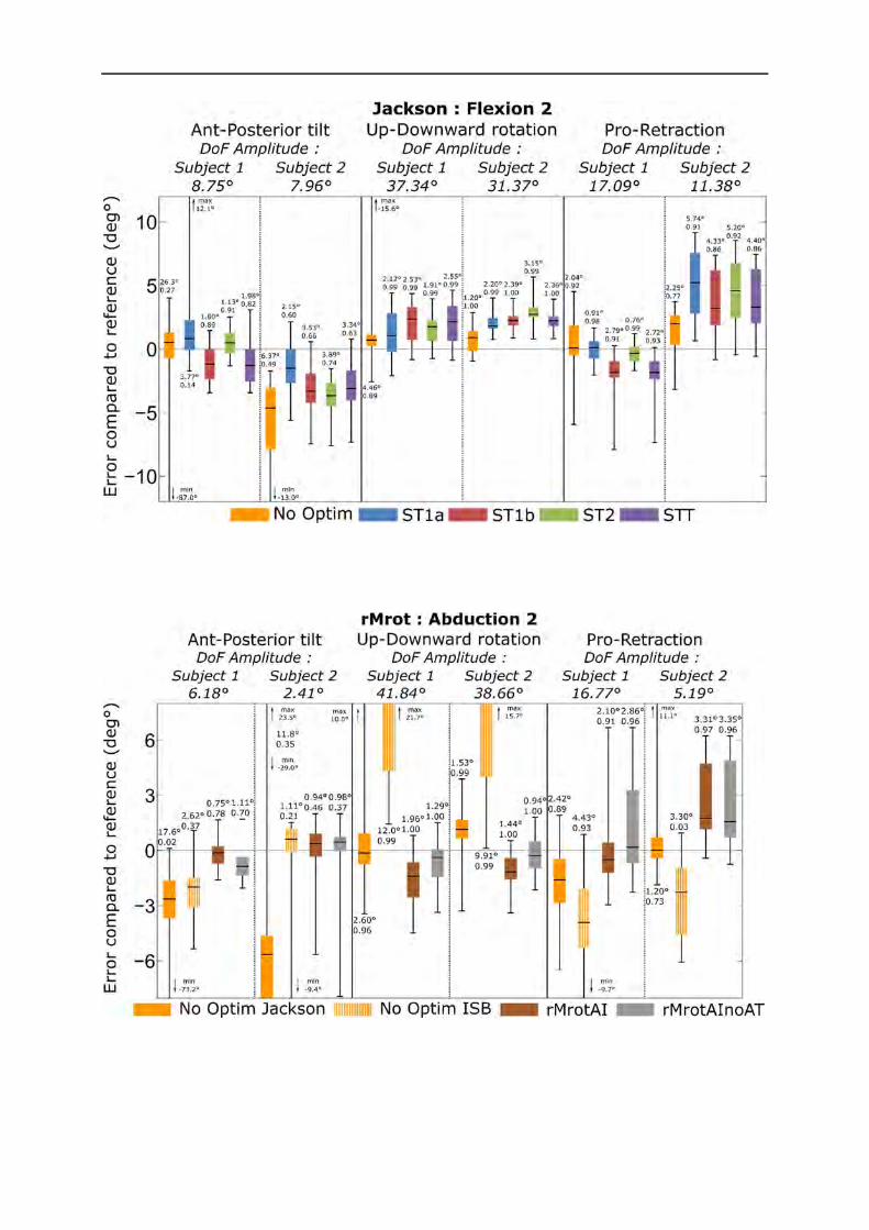
Appendix
150
Figure 85 : Boxplots of the error existing between the bones kinematics and the different models kinematics using the Jackson et al. markers set as motor constraints for the anterior-posterior tilt, the
upward-downward rotation and the protraction retraction during a flexion movement
Figure 86 : Boxplots of the error existing between the bones kinematics and that obtained using different markers set for the anterior-posterior tilt, the upward-downward rotation and the protraction retraction
during an abduction movement
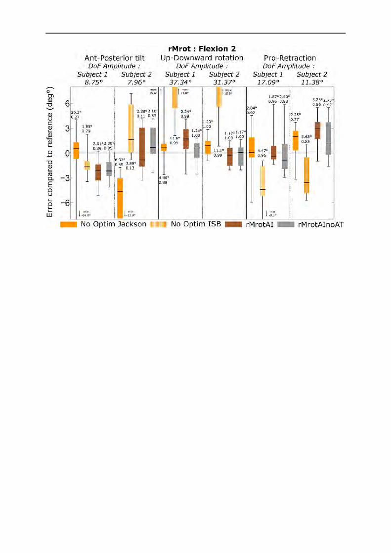
Appendix
151
Figure 87 : Boxplots of the error existing between the bones kinematics and that obtained using different markers set for the anterior-posterior tilt, the upward-downward rotation and the protraction retraction
during a flexion movement


