Advanced Foundation Engineering Prof. Kousik Deb

Department of Civil Engineering Indian Institute of Technology, Kharagpur

Lecture - 18

Pile Foundation- Load Carrying Capacity-II

In last class I have discussed about the how to calculate the pile load capacity by using

pile load test, so now in that class I have discussed about the total load carrying capacity

of the pile, I will calculate the total allowable load carrying capacity of the pile by using

pile load test.

Now, if we want to know the contribution from the tip resistance, and the friction

resistance friction part separately, then we have to go for the cyclic pile load test. Now,

in this section I will discuss about the cyclic pile load test, and how to determine the

frictional resistance of the pile, in the tip resistance of the pile based on this cyclic pile

load test.

(Refer Slide Time: 01:02)

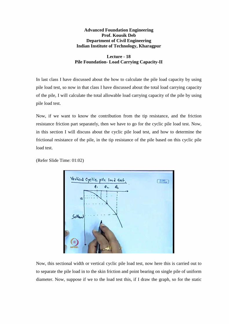
Now, this sectional width or vertical cyclic pile load test, now here this is carried out to

to separate the pile load in to the skin friction and point bearing on single pile of uniform

diameter. Now, suppose if we to the load test this, if I draw the graph, so for the static

load we will draw we will get say these are the different load Q 1, this is Q 2, and the say

this is Q 3, so these are the increment, different increment Q 1, Q 2, Q 3.

And there, because we are applying the load in 20 percent of increment, so there this is

the load corresponding settlement, that I will measure; similarly this is the load and

corresponding settlement that we will measure, so this is the value and this is the load

and corresponding settlement this will measure (Refer Slide Time: 02:15). So, this is our

if I join this point, so this will give us the static pile load test, and there so this will give

up the this is the load and this is the settlement; so this settlement this will give us the

static load pile load test curve.

Now, similarly here once we get this, this type of graph, so and then the others Q 4 and

Q 3, Q 5 then we will get the complete the graph, and then if we want to determine the

allowable load carrying capacity of the pile, then we have to apply those conditions.

Suppose, 1 is a 2 3 rd of the load by which the settlement attains a value of 12

millimeter, suppose this is 12 millimeter then we will calculate suppose this is the load

12 millimeter, then we will calculate the q value corresponding 12 millimeter, and then

we will take the 2 3 rd of that load (Refer Slide Time: 03:27).

Similarly, we go for the second condition, then we will go for 50 percent of pile

diameter, then we will get one settlement corresponding load 10 percent of the pile

diameter for the uniform loaded pile, and then we will go for the that Q and take the 50

percent of that. Then similarly, we have to consider the all the condition and the

minimum of that Q will consider that is the allowable load carrying capacity of the pile,

but there we cannot know what the contribution from the skin friction is, and what the

contribution from the tip resistance.

Where we there we are getting another total load carrying capacity or allowable load

carrying capacity of the pile. Now, here by the cyclic test, we will calculate, we will

know what would be the contribution from the friction resistance, and what would be the

contribution from the tip resistance.

(Refer Slide Time: 04:28)

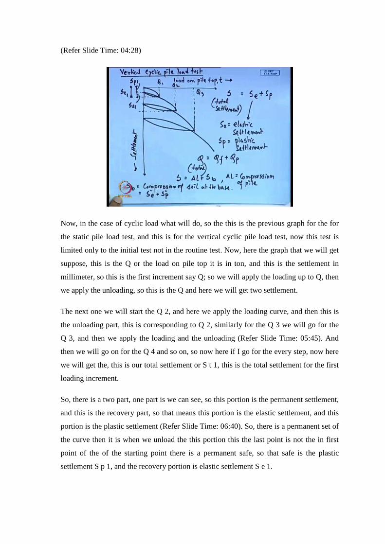
Now, in the case of cyclic load what will do, so the this is the previous graph for the for

the static pile load test, and this is for the vertical cyclic pile load test, now this test is

limited only to the initial test not in the routine test. Now, here the graph that we will get

suppose, this is the Q or the load on pile top it is in ton, and this is the settlement in

millimeter, so this is the first increment say Q; so we will apply the loading up to Q, then

we apply the unloading, so this is the Q and here we will get two settlement.

The next one we will start the Q 2, and here we apply the loading curve, and then this is

the unloading part, this is corresponding to Q 2, similarly for the Q 3 we will go for the

Q 3, and then we apply the loading and the unloading (Refer Slide Time: 05:45). And

then we will go on for the Q 4 and so on, so now here if I go for the every step, now here

we will get the, this is our total settlement or S t 1, this is the total settlement for the first

loading increment.

So, there is a two part, one part is we can see, so this portion is the permanent settlement,

and this is the recovery part, so that means this portion is the elastic settlement, and this

portion is the plastic settlement (Refer Slide Time: 06:40). So, there is a permanent set of

the curve then it is when we unload the this portion this the last point is not the in first

point of the of the starting point there is a permanent safe, so that safe is the plastic

settlement S p 1, and the recovery portion is elastic settlement S e 1.

Similarly, for the second set also this there is a two part one is the total, so from this is

the total, and then this is the plastic settlement, and this is the elastic settlement (Refer

Slide Time: 07:33). So, now every increment of loading will get one plastic settlement,

one elastic settlement that is for every increment.

Now, if I write the settlement of the total settlement if S is the total settlement, so that is

total settlement is the summation of elastic settlement plus summation of plastic

settlement, so S e is the elastic settlement, where S e is the elastic settlement and S p is

the plastic settlement. Similarly, the total Q that we are getting that is the combination of

friction resistance and the tip resistance. And we can write, so that elastic settlement and

the combination of the summation of elastic settlement, and plastic settlement is the, is

the total settlement, total load is the summation of friction resistance plus the tip

resistance.

In other hand, we can write the total settlement is the summation of del L plus S b, so

now where del L is equal to compression of pile material, pile or pile material. And S b

is compression of soil at the base (No audio from 09:43 to 09:56), so that this is also S b

have two component elastic part and plastic part, so this is the elastic part and the plastic

part.

So, we can say this is the S is the total settlement that is the elastic settlement total elastic

settlement and total plastic settlement, and here if that will get the compression of the

pile material, because that class the compression of the soil at the base (Refer Slide

Time: 10:21). So, at the base soil also so that means, the the total settlement it is due to

the summation of the, the soil settlement at the base, so base soil that will settle, because

of that we will get the settlement of the pile, and the pile material that may also

compress.

So, that is the summation of the compression of the pile material, and the compression of

the base soil, similar the base soil also there is two types of settlement, one is elastic

settlement, another is the plastic settlement. So, and in the pile material also we can

consider two types of settlement, one is the plastic settlement and the elastic settlement.

So, the total elastic settlement is the summation of elastic settlement of the pile material,

and the elastic settlement of the base soil. And total plastic settlement is the plastic

settlement of the pile material, and plus the plastic settlement of the base soil.

(Refer Slide Time: 11:47)

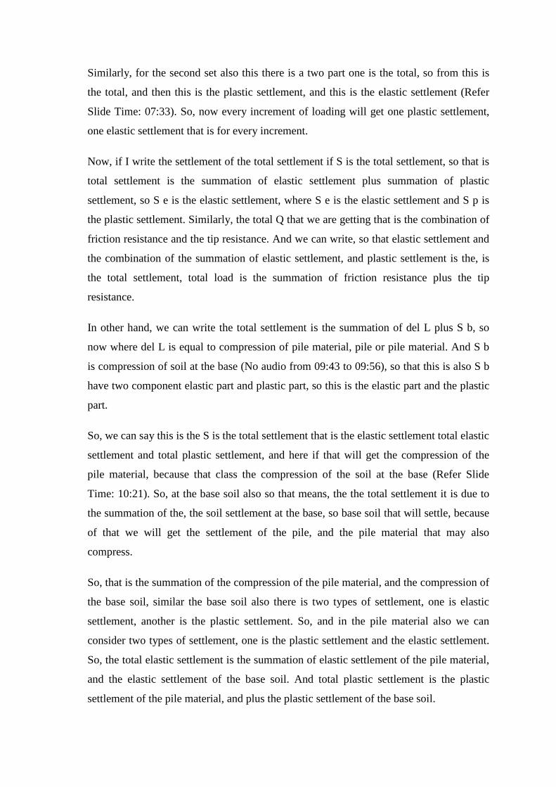
Now, here if I further write this expression in different form, then we will get that again

we can write this S p dash is the plastic compression of the soil at the base, S elastic

compression of the soil at base, and S p dash is the elastic compression of the soil, this is

the plastic compression of the soil at the base. So, finally we can write the total

settlement is del L plus S e dash plus S p dash, and again we have written that S is total

elastic settlement plus total plastic settlement.

So, if I compare this to expression, so S e plus S p that will be del L plus S e dash plus S

p dash. So, you can write that S e dash elastic settlement at the base is S p minus S p

dash plus S e minus del L, now this S p and S e that we can determine from the figure or

the pile load test that load versus settlement figure. And this if I this del L we can

calculate by this expression that Q minus Q f by 2 into L divided by A E, where Q is

equal to total load on the pile Q f, the frictional resistance, frictional load or resistance

(Refer Slide Time: 13:30).

This is the length of the pile (No audio from 14:14 to 14:21) (Refer Slide Time: 14:14),

this is the average cross section area of the pile, E is the modulus of elasticity of the pile

material of the pile material, so this is the is the modulus of elasticity of the pile material.

Now, if we consider that the plastic settlement of the pile material is negligible, because

the plastic settlement, total plastic settlement we are taking the summation of plastic

settlement of the pile material, and plastic settlement of the base soil.

So, here we assume the plastic settlement of the pile material is negligible, so we are

taking the all the settlement of the pile material is elastic, because the pile material is

very steep compare to the soil. So, the plastic settlement is, plastic settlement of the pile

material is negligible, so total settlement will be total plastic settlement will be plastic

settlement of the base soil, because plastic settlement of pile material is neglected as (No

audio from 15:59 to 16:13) is neglected, in that case S p will be S p dash.

So, from this expression, so if I write this is equation 1, so from equation 1 we can write,

or equation this is 1 we can write that S e bar is S e minus del L, so this is the expression

or the final expression. So, here del L we will calculate by this expression, and S e we

have to determine from the pile load load versus settlement graph, and then we will

calculate the S e part.

Now, the next step how to determine the Q f and Q p; the next step determination of Q f

and Q p…

(No audio from 17:20 to 17:36)

(Refer Slide Time: 17:20)

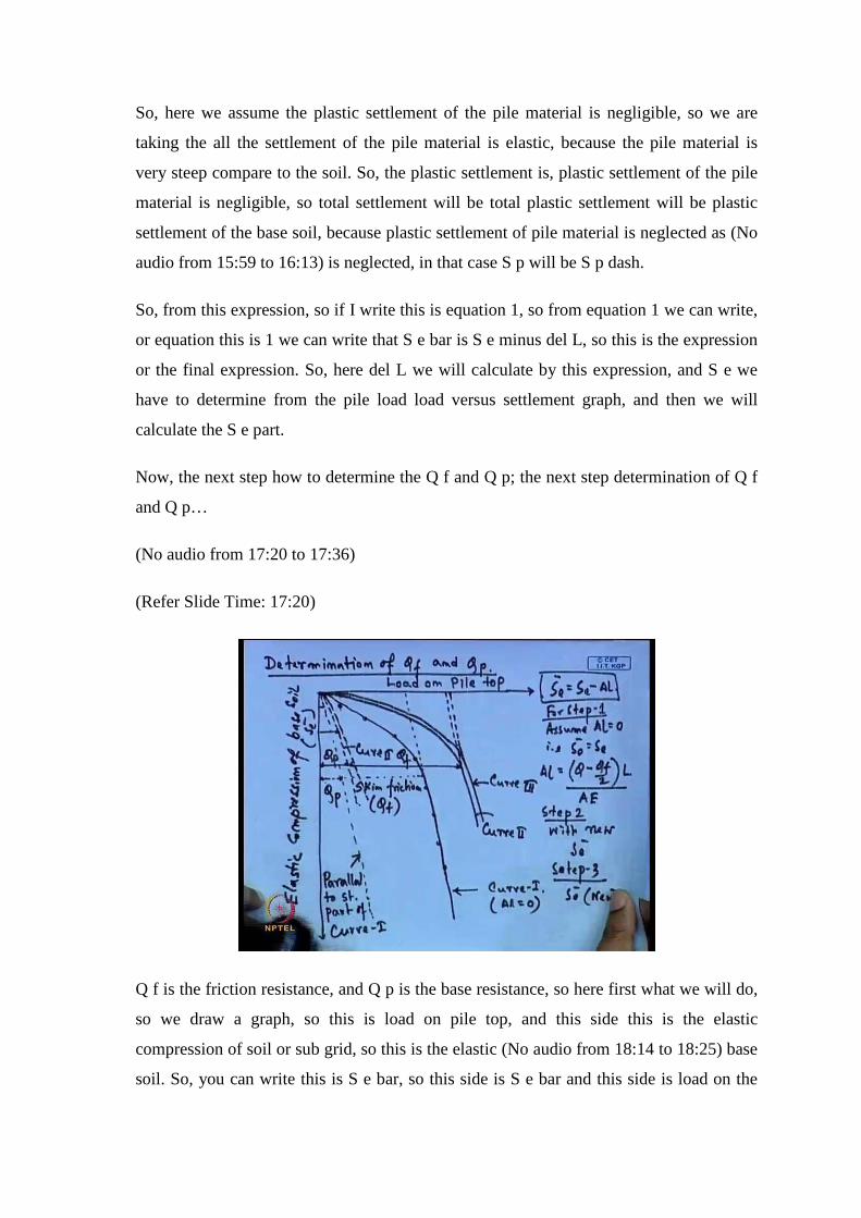
Q f is the friction resistance, and Q p is the base resistance, so here first what we will do,

so we draw a graph, so this is load on pile top, and this side this is the elastic

compression of soil or sub grid, so this is the elastic (No audio from 18:14 to 18:25) base

soil. So, you can write this is S e bar, so this side is S e bar and this side is load on the

pile, so first step we assume that del L is 0, so what we will get from this load versus

settlement curve or the first curve, so that I have drawn this for the pile.

So, from this first curve we will get what is the S e for a particular loading density, for a

particular loading density what is S e (Refer Slide Time: 19:01). Now, if we consider that

because the our expression is S e bar equal to S e minus del L, so that is the expression

and for the first step, for the step 1 assume del L is equal to 0, so this S e for any load

increment will get from the previous curve or load versus settlement curve, and then we

will get the S e.

So, in that case S e that is S e bar is equal to S e for the first step, this is for the first step

only, so what we will do now we will draw this graph, corresponding to different loading

point (No audio from 20:12 to 20:22), so we will draw this graph, so this is say curve I,

this is for the first step where we assume that del L is equal to 0 (Refer Slide Time:

20:00).

Under next step that what we will do that, we will draw one line which is parallel to this

straight portion, now this is the straight portion of the graph, so here we will get one non-

linear portion, then is a straight portion of the graph. And we draw one parallel line

which is passing through this origin, and parallel to this straight portion of this curve I

(Refer Slide Time: 21:16). So, which is passing through the origin, and this is this graph

is parallel to the straight line portion of curve I, so this is parallel parallel to straight part

of curve I.

Now, from this graph we will determine what would be the value of here, from this

graph, so this part will give you the point resistance of any loading increment for this

loading increment say (Refer Slide Time: 22:00). So, this will give the point resistance

and this part will give the friction resistance, this is the skin friction or Q f, and this is the

Q b part Q b or p part. So, or any loading position say from this portion, here this portion

is Q p and for this is the friction resistance part, so here that we will determine.

So, once we get this any loading condition will get the Q p and Q f, in the second step

once we know the Q a value, because that expression of del L, del L we are giving that is

the Q minus Q f divided by 2 into L divided by A E. So, E is material property L is the

length of the pile, and Q and Q is the total load at load or the load increment at any point,

and once we get the Q f from this part, because this step portion this step portion left

hand side will give you the Q p and this is the right hand side will give us the Q f (Refer

Slide Time: 23:29)

So, once we get the Q f at any loading increment from this graph, will get the del L, so

for the any loading increment we will calculate the del L, and that del L we will put here,

and S e is previously we can calculate from the load (( )) displacement curve and that is

the same as the step I. So, now we will get the new S e bar, so once we get a new S e bar

then we will draw another curve by using the new S e bar, suppose that is this curve is

the new S e bar or the step II (Refer Slide Time: 24:16).

So, this is our step II, how do we calculate new S e with new S e bar, so this is say curve

II similarly, this curve also we will get one straight portion we extend this, straight

portion of the curve, and again we will draw the parallel line of this straight portion, so

this is the parallel line for curve II (Refer Slide Time: 24:39). And similarly, we will

repeat the something here also we will get the Q p and Q f separately from this, the left

hand side of this part, so this portion is basically this portion is Q p, and this portion is Q

f.

So, this here also this is Q p, the Q f the Q p and Q f for the first part and this is this

portion is Q f and this portion that means, the right hand side of this straight line which is

passing through the origin straight parallel to the straight portion of the curve, right hand

side of this curve is Q f, and left hand side of this curve is Q p. So, once we get this value

then we will calculate the new del L, and then we will get the new again in the step 3, we

will get another S e bar or the new S e bar, then will get another we will calculate

another curve (Refer Slide Time: 25:59).

So, this is our curve III and again we will extend this the straight portion, and then we

will again draw this parallel line for the straight portion of this third curve, and again we

calculate the Q p and Q f, again we repeat the something, we will calculate new del L we

will calculate the new S e bar. And we will repeat the thing unless the two curves are ((

)) curve were matching each other, and generally it is observed the after the three trails

this curves are matching each other.

So, this so when this curves are matching say suppose curve III and curve IV are

matching each other, then we will stop there. And then from that curve itself, similarly

from this straight portion right left hand side will give us the contribution from the Q p

that means, this is left hand side. And the right hand side of this straight portion which is

passing of the of the line which is passing from this origin, right portion right hand side

of this curve up to the origin original curve that will give us the friction resistance.

So, one the so for this method we can determine, what is the contribution from the tip

resistance, and friction resistance separately. Now, this will give us the ultimate load

carrying capacity of the friction or contribution from the friction and the tip separately

(Refer Slide Time: 27:45). Now, if we want to find the safe pile capacity, then you have

to divide this thing by factor of safety.

Now, for the skin friction resistance, so that we if we divide this part by factor of safety,

we will get the safe friction resistance, and safety bearing resistance that we are getting

from this pile, by that we can determine from the pile load test. So, by this method the

cyclic pile load test, we can separately determine the contribution from the friction part

or friction resistance and from the tip resistance of the pile by this pile load test.

Now, the next section that on the, next section we will discuss about the pile load test for

the different dynamic pile formula, because this is the third method, because the first

method was static expression. Now, this second one data I have discussed from the pile

load test, now next one that we will discuss that I will discuss that is five dynamic pile

formula.

(Refer Slide Time: 29:02)

So, this is the (No audio from 29:01 to 29:12) over that one formula that will given, so

first one will giving the (No audio from 29:17 to 29:24) engineering news record or ENR

formula. So, these are the based one the pile driven energy or the weight that we are

using, based on that we are calculating this allowable load carrying capacity of the pile.

So, Q allowable or the allowable pile load that we can calculate by W into H into sigma

H into S plus C, where W is weight of the hammer (No audio from 30:22 to 30:37). And

H is the height of fall (No audio from 30:43 to 30:53) height of falling, S is the real set

per blow, C is the empirical factor, F is factor of safety usually taken as 6 and this is the

efficiency.

Now, for the drop hammer this value is 0.7 to 0.9, for steam hammer this value is 0.75 to

0.85. So, now, this equation of this expression is based on the energy that we are

applying to or to drew and drive a pile into the soil. So, this is the weight of the hammer

this is the free fall height this efficiency and this is a factor of safety, which is generally

taken of 6, S is the set real set per blow. Before we apply the load how much is the

amount of the real set per blow that is S and C is the empirical factor. Now, this

expression we can use for different hammer.

(Refer Slide Time: 32:48)

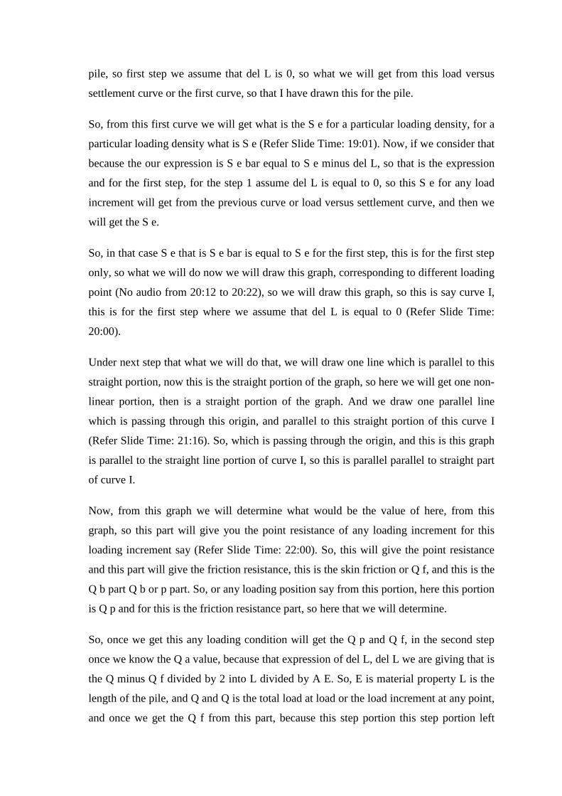
So, now, for the drop hammer (No audio from 32:46 to 32:55) this Q a is W into H and

this is the efficiency into 6 factor of safety and S plus 2.5. This is for the drop hammer

where q a, and w this is in k g, H in centimeter, S is equal to centimeter per blow that is

the final set or the real set or the final set (No audio from 33:34 to 33:45).

So, this final set S we can take, that S value that the average penetration, (No audio from

33:52 to 34:02) for the last 5 blows of a drop hammer or 20 blows of a steam hammer.

So, that means this S centimeter per blow, here the final set when last 5 blows average

that, we will consider as the S in case of drop hammer. And for last 20 blows of in case

of steam hammer, the average of last 20 blows penetration that we will consider the s

value in case of steam hammer.

So, similarly for the steam hammer or single acting steam hammer, this Q a is equal to W

into H into efficiency by 6 plus S into 0.25. So, here for the drop hammer c value is 2.5,

for the steam hammer this is 0.25. So, this again this W and Q a is in k g H is in

centimeter, S in centimeter per blow this is 0.25.

So, by using this expression also we can determine the pile load carrying capacity of the

pile. So, now, there is others other this type of expression are also available, but here I

am just giving one expression, which is very popular that is the a ENR formula and by

which we can also determine the pile load carrying capacity. The next one the fourth

method, that we can determine the pile load test by using the correlation with the

penetration test data.

(Refer Slide Time: 36:35)

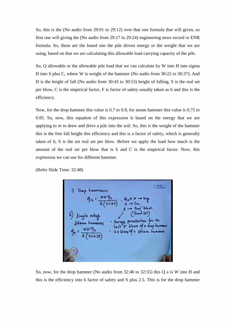
By using (No audio from 36:31 to 36:41) with penetration test value; that means, by SPT

or CPT value we can determine the pile load carrying capacity of the pile. Now first we

will given the for the driven pile in sand, so driven pile in sand. So, here q p u that

means, the it is the tip resistance ultimate tip resistance (No audio from 37:25 to 37:37).

That this 40 N into L by D which is in kilo Newton per meter square, but that should be

less than equal to 400 N kilo Newton per meter square. That means, this if we use this

expression, now that q u p cannot be greater than 400 N kilo Newton per meter square.

So that means, if it is coming more than 400 kilo Newton per meter square, N kilo

Newton per meter square, then we have to consider the 400 N kilo Newton per meter

square.

So, that means, so this will limited to this value that means, this is the ultimate tip

resistance. Similarly, for the driven pile we can find the q p u that is q c, which is based

on the SPT value, this is the SPT value. So, this is SPT value is observed value without

any correction. So, this N is observed value without any overburden correction

correction.

Now, again by the q c that means, the cone resistance, this is the cone resistance, we can

determine the tip ultimate tip resistance of the pile. Now, q c is taken as the average

value q c over a distance 3 D above and 1 D below the level of the pile tip. That means,

this q c value, suppose this is the pile tip portion and this diameter is say D. So, that we

can take the average value of this is 3 D and 1 D, then this is the tip.

So, the average value of this 4 D portion, the 3 D above the tip and 1 D below the tip that

average value of q c, that we have to consider as this q c. So, that means, for the pile to

attain the it is full bearing resistance it should be driven at least 5 D inside the bearing

strata. For the pile attain its full bearing resistance; that means, for the pile attains the full

bearing resistance it should be driven at least 5 D inside the bearing strata. Suppose, if

there is a bearing strata is there.

So, this is suppose the bearing strata inside this one is the bearing strata, bearing layer

then the pile this has to be penetrated inside the strata at least for the 5 D part. Then we

will get the full resistance this is the at least. See, if one pile is penetrated that this

bearing layer or the bearing strata at least for the 5 D length then we will give the full

resistance from this strata. Now that means, here the this q c value will take the average

of this 3 D above the tip and 1 D below the tip this average of this 4 D zone, we will get

the q c.

Average q c will give the q c and if we get the full resistance of this any bearing strata,

then this bearing strata this pile has to be penetrated at least 5 D below this within this

bearing strata. Now, the friction resistance this is the we are talking about the ultimate tip

resistance then how to get the friction resistance.

(Refer Slide Time: 42:08)

The friction resistance of the pile, (No audio from 42:08 to 42:17) so for the driven pile

here the same thing for the driven pile in sand. So, we are talking about the this pile in

sand, the friction resistance f s we can take the q c average by 2 that is in kilo Newton

per meter square.

And this is for the, this is displacement pile or this is for the displacement pile and f s is

equal to q c average by 4, this is kilo Newton per meter square this is for the H pile. This

expressions are given by the both the expressions given by the Meyerhof in 1956. Now,

q c average, is the average cone resistance (No audio from 43:35 to 43:45) along the

length of the pile, this is the average cone resistance along the length of the pile same

way.

Similarly this is in terms of cone resistance, similarly for the in terms of N value this q s

is equal to 2 N average this is also kilo Newton N meter square, this is for the

displacement pile or q s equal to N average that is in kilo Newton per meter square this is

for the H pile. Where N average this is the SPT value this is the average field value of N

this is the SPT along the length of the pile.

Now, another condition that, here the for the q p even that means, the tip resistance also

that that cannot be greater than 400 N value. Similarly, now for the displace q f s that is

less than equal to 100 kilo Newton per meter square, this is for the displacement pile and

that is less than equal to 50 kilo Newton per meter square that is for the H pile. So, this is

the another two condition, so these are the expression for the driven pile in the sand.

(Refer Slide Time: 46:04)

Next one we will give the expression for the bored and cast in situ pile in the sand. This

is the bored, (No audio from 46:05 to 46:27) now again we will get the q p u that is equal

to 1 3 rd of q p u that we will get of driven pile. And f s that is equal to half of the f s of

driven pile. So, first we will calculate the q q p u and f s for the driven pile, and then we

take the 1 3 rd for the bored and cast in situ piles in sand and f s is half of the f s of the

driven pile.

Next one is the driven and cast in situ pile. Now here for the case pile, case pile it is

same as driven pile. And for the uncased pile the f s as driven pile if a case f s is same as

driven pile. Now, if proper compaction is done or either we can take f s as bored cast in

situ pile, if proper compaction is not done. So, these are the condition or these are the

condition by which we can determine the pile load carrying capacity of the pile or as the

tip resistance of the pile or the friction resistance of the pile, based on the penetration test

data; that means the cone resistance or the n value or the SPT n value. We can determine

this for the driven pile, we can determine bored cast in situ pile, we can determine for the

driven cast in situ piles also. And that then in the different pile condition in the case pile

uncased pile on all this the cases, we can driven we can determine the pile load capacity

of the pile by using this penetration value.

So, there is four different methods by which we can determine the ultimate load carrying

capacity of the pile or allowable load carrying capacity of the pile, one first one is the

static method or static equation or the formulae. Next one, second one is the by the pile

load test, so for the for the static or the cyclic if I go for the for the cyclic pile load test

then we can determine separately the section resistance and the tip resistance. And third

one by using the dynamic equations or the formulae’s and formulae. And the next one in

the third expression is by using by using the penetration test data.

So, these are the all different methods by which we can determine the pile load,

ultimately pile load capacity of the pile different piles. And then in the in this section I

have also discussed, that when we go for the group analysis or group calculation, then

how we will calculate this group efficiency of the pile and group ultimate load carrying

capacity of the pile.

Now, this in the next section I will discuss about the settlement of the pile, then the how

to calculate the load bearing capacity of the under reamed pile in those things, I will

discuss in the next section.

Thank you.