Advanced Design for Mechanical System Pract10 1 Thermal analysis There is a resemblance between the...

Advanced Design for Mechanical System Pract10

1

Thermal analysis

•There is a resemblance between the thermal problem and the stress analysis.

•The same element types, even the same FE mesh, can be used for both analysis

•Thermal analysis means primarily calculation of temperature within a solid body

•A by-product of the temperature calculation is information about the magnitude and direction of heat flow in the body.

•The results of thermal analysis, nodal temperature, can be used to evaluate the distribution of stresses due to the presence of a thermal gradient within the body


2

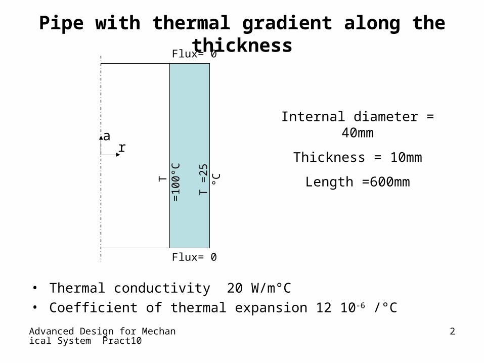
Pipe with thermal gradient along the thickness

T =

25 °

C

T =

100°

C

• Thermal conductivity 20 W/m°C• Coefficient of thermal expansion 12 10-6 /°C

Internal diameter = 40mm

Thickness = 10mm

Length =600mm

Flux= 0

Flux= 0

ra


3

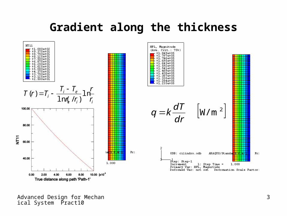
Gradient along the thickness

iie

eii r

r

rr

TTTrT ln

)/ln()(

2W/m dr

dTkq


4

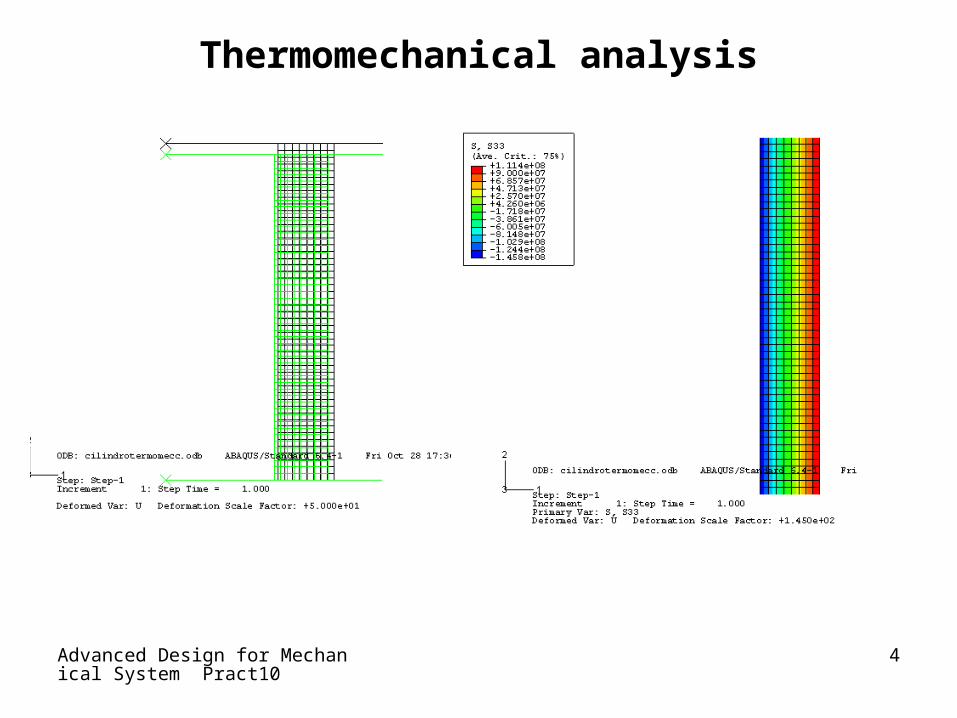
Thermomechanical analysis


5

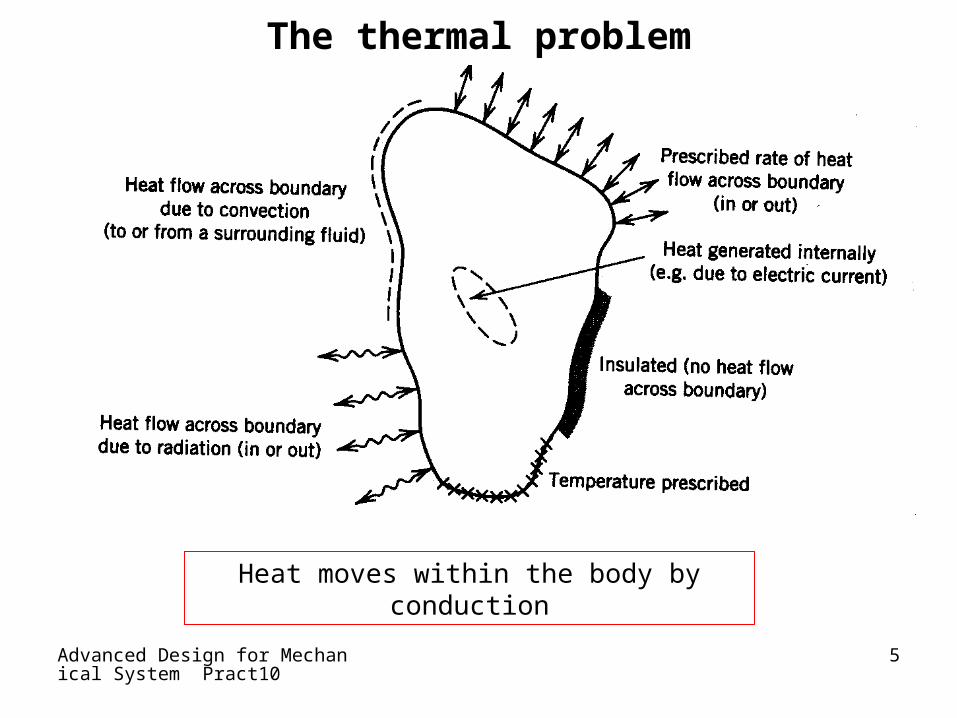
The thermal problem

Heat moves within the body by conduction


6

Fourier equation of heat flow

fx, heat flux for unit area (W/m2)

k thermal conductivity (W/m°C)

Negative sign means that heat flows is in a direction opposite to the direction of temperature increase

The temperature represents the potential for the heat flow.

Consider an isotropic material and image that exist a temperature gradient in the x direction

x

Tkf x


7

zT

yT

xT

f

f

f

x

Tkf

z

y

x

x κ

fx, fy, fz heat flux for unit area (W/m2)

matrix of thermal conductivity (W/m°C)

Boundary condition on surface with normal n

s

SnS

fn

TkTT

f

Hp: non isotropic material

the direction of the heat flow in general is not parallel to the direction of the temperature increase


8

Conductivity

•The matrix of conductivity is in general a full 3 by 3 matrix

•If x,y,z are principal axes of the material is a diagonal matrix

•In the special case of isotropy 11=22=33=


9

t

Tcq

f

f

f

v

z

y

x

zyx-

By considering a differential element of volume dV and writing the balance equation (rate in – rate out)= (rate of increase within), it is obtained:

where:

qv is the rate of internal heat generation for unit volume (W/m3)

c is the specific heat (J/kg °C)

is the density (kg/m3)

t is the time (s)


10

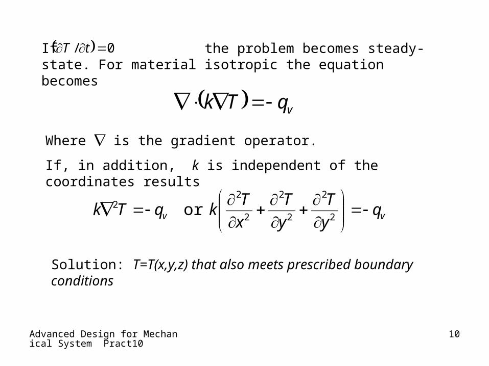
If the problem becomes steady-state. For material isotropic the equation becomes

vqTk

vv qy

T

y

T

x

TkqTk

2

2

2

2

2

22 or

0/ tT

Where is the gradient operator.

If, in addition, k is independent of the coordinates results

Solution: T=T(x,y,z) that also meets prescribed boundary conditions


11

• The heat flow trough the surface of the body is analogous to surface load in the stress analysis.

• A distributed internal source is analogous to body forces in stress analysis.

• Prescribed temperature are analogous to prescribed displacements• For a steady state problem, the mathematics of all this leads to the

global FE equation

QTKT

where:KT depends on the conductivity of the material ([W/°C])T is the vector of the nodal temperature ([°C])Q is the vector of the thermal loads ([W])

•Convection and radiation boundary conditions, if present, contribute term to both KT and Q.


12

Hypothesis for FE in thermal analysis

• In solid body the heat transfer occurs by conduction

• In fluid the transmission by mean of convection must be take into account

• In many structural problems the thermal problem and the mechanical problem are not coupled

• This hypothesis is no longer valid when the deformation can generate heat and cause a variation of the mechanical properties

• Thermal conductivity and other properties of the material must be considered dependent on the temperature

• The conductivity matrix can be generated by a direct method for very simple elements, otherwise a formal procedure is required


13

Thermal bar element

The rate of heat flow, q=Af, is constant and direct axially.

T1>0, T2=0 T2>0, T1=0

Nodal heat flow is positive when direct within the element

An actual bar can be modeled by several of these elements if temperature at several locations between its ends were required


14

2

1

2

1

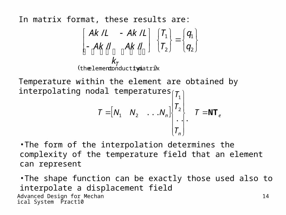
matrixty conductivielement the

//

//

q

q

T

T

k

lAklAk

LAkLAk

T

In matrix format, these results are:

Temperature within the element are obtained by interpolating nodal temperatures

e

n

n T

T

T

T

NNNT NT

...

... 2

1

21

•The form of the interpolation determines the complexity of the temperature field that an element can represent

•The shape function can be exactly those used also to interpolate a displacement field


15

NB BTT

y

x

T

T

T

yNyNyN

xNxNxN

yT

xT

n

n

n

/

/ where

.../...//

/...//

/

/ 2

1

21

21

volumeelement

dVk TT κBB

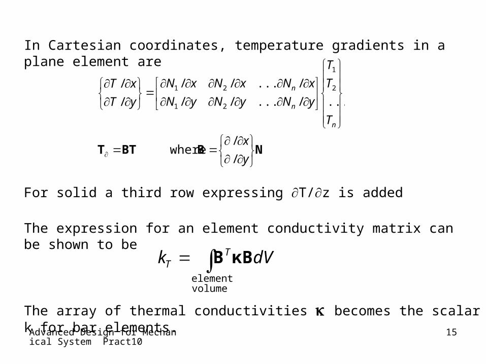
In Cartesian coordinates, temperature gradients in a plane element are

For solid a third row expressing T/z is added

The expression for an element conductivity matrix can be shown to be

The array of thermal conductivities becomes the scalar k for bar elements.


16

Remarks•The thermal problem is a scalar field problem

•A FE temperature field is continuous within elements and across interelement boundaries

•Temperature gradient, like strains in stress analysis, are typically not interelement continuous

•If radiation is not present, the rate of heat flow is proportional to temperature differences

•Upon assembly of elements, nodal rates of heat flow qi from separate elements are combined at shared nodes.

•Thus the net flow into node i of the structure:

except at nodes where Ti is prescribed, nodes on a structure boundary across which heat is transferred, or at internal nodes where Qi arise from qv

0 ii qQ


17

Where

f is the flux normal to the surface and positive inward

h is the heat transfer coefficient

Tf e T temperature of the fluid and of the surface of the body

For the increment, dS, of the element surface subjected to convection formal procedure gives

The matrix combine with the element conductivity matrix and hence contribute to KT the vector contribute to Q

Convection boundary conditions

)( TThf f

dShThdS fTT NNN :tor vec:matrix

If the material conductivity is dependent on temperature a nonlinearity is present


18

Radiation boundary conditions

44

44

fluxheat radiated

4

fluxheat received

4

1)/1()/1(TTf

TTTTf

rr

SB

rSBSBrSB

Consider two infinite parallel planes. Let the planes have temperature Tr and T , and each is a perfect absorber and perfect radiator (black body).

If SB is the Boltzman constant, the net heat flux received by the surface at temperature T is

If the emissivity (ratio of total emissive power to that of a blackbody at the same temperature) is introduced, than


19

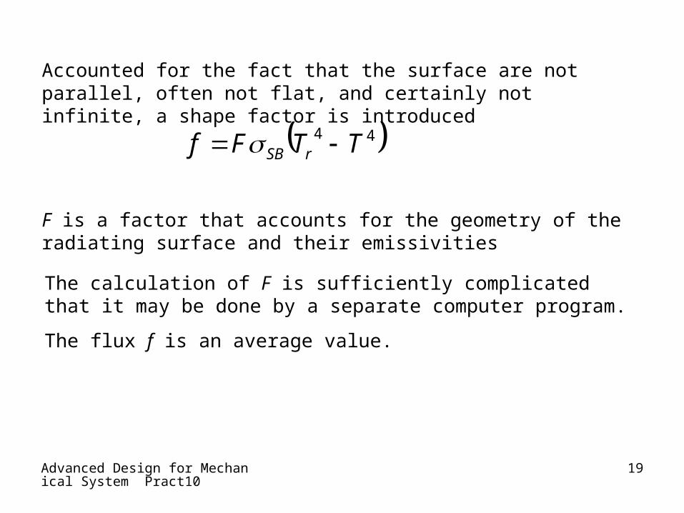
Accounted for the fact that the surface are not parallel, often not flat, and certainly not infinite, a shape factor is introduced

F is a factor that accounts for the geometry of the radiating surface and their emissivities

44 TTFf rSB

The calculation of F is sufficiently complicated that it may be done by a separate computer program.

The flux f is an average value.


20

TTTTFhTThf rrrrr 2244 dove

This equation can be written as

T is the absolute [K]

hr= hr(T) is a temperature dependent heat transfer coefficientThis makes the problem non linear and requires iterative solution

•The flux expressions have the same form for convection and radiation boundary conditions

•Accordingly, a radiation boundary condition leads to matrix and vector expressions having the same form as for convection, with h and Tf replaced by hr and Tr


21

Modeling considerations

• Element types, and shapes for a thermal analysis may be dictated less by thermal analysis than by an anticipated stress analysis based on the same mesh

• The mesh demands of stress analysis are usually more severe

• Also a modest temperature gradient may create forces of constraint that produce large strain gradients, especially near holes, grooves and other stress raisers.

• Also for thermal analysis the present symmetry must be considered: heat flux trough a plane of symmetry is zero

• Heat flux must be parallel to an insulate boundary or a plane of symmetry

• Temperature contours (isotherms) should be parallel to a boundary of constant temperature and normal to plane of symmetry


22

Non linearity

• If in the body there are appreciable difference of temperature, it is necessary to regard conductivity as temperature dependent

• If there is convection with a temperature dependent coefficient of heat transfer

• If is present radiation

)()(

)(

)(

TT

TQQ

TKK TT

QTKT

The problem is non linear


23

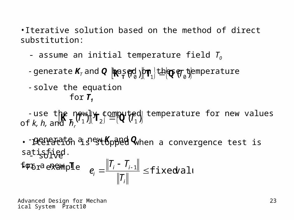
• Iteration is stopped when a convergence test is satisfied.

•For example

valuefixed1

i

iii T

TTe

•Iterative solution based on the method of direct substitution:

- assume an initial temperature field T0

- generate KT and Q based on these temperature

- solve the equation for T1

- use the newly computed temperature for new values of k, h, and hr

- generate a new KT and Q

- solve for a new T )()( 121 TT QTKT

)()( 010 TT QTKT


24

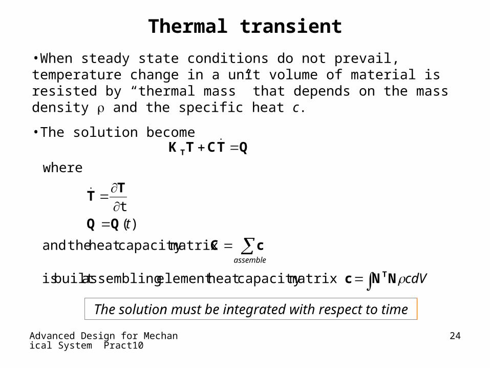
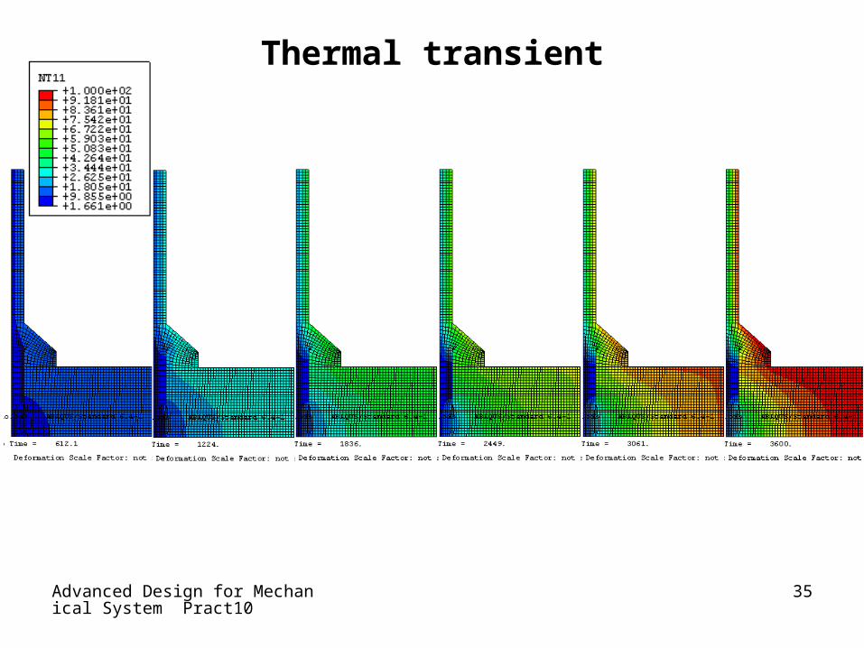
Thermal transient

cdV

t

assemble

NNc

cC

QQ

TT

QTCTK

T

T

matrix capacity heat element assembling built is

matrix capacity heat the and

t

where

)(

The solution must be integrated with respect to time

•When steady state conditions do not prevail, temperature change in a unit volume of material is resisted by “thermal mass” that depends on the mass density and the specific heat c.

•The solution become


25

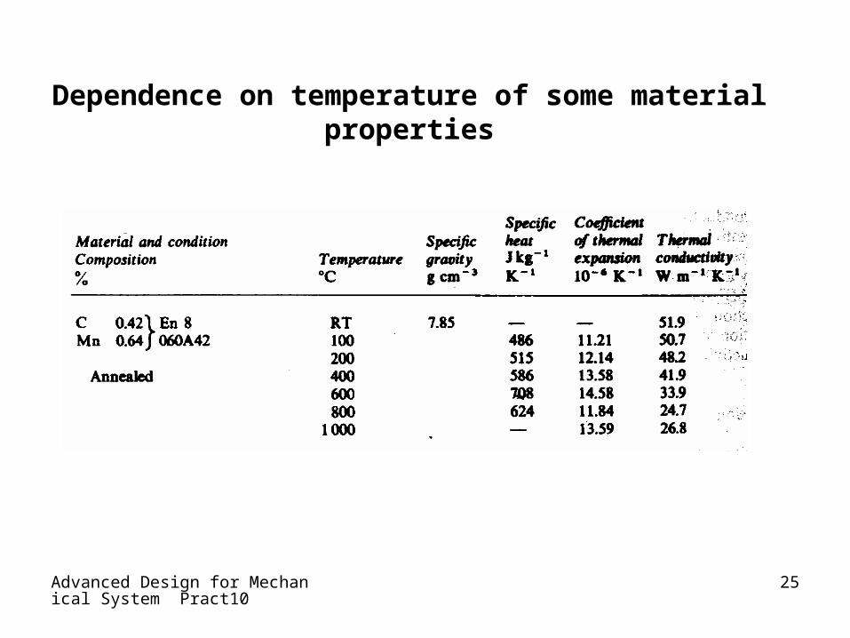
Dependence on temperature of some material properties


26

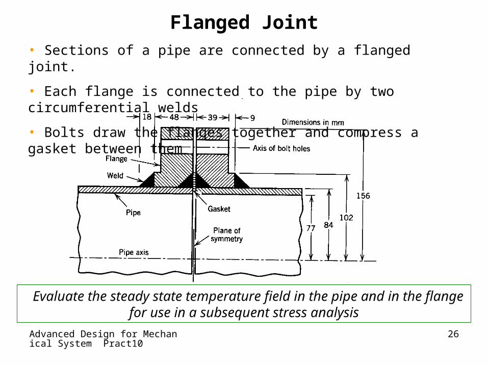
Flanged Joint• Sections of a pipe are connected by a flanged joint.

• Each flange is connected to the pipe by two circumferential welds

• Bolts draw the flanges together and compress a gasket between them

Evaluate the steady state temperature field in the pipe and in the flange for use in a subsequent stress analysis


27

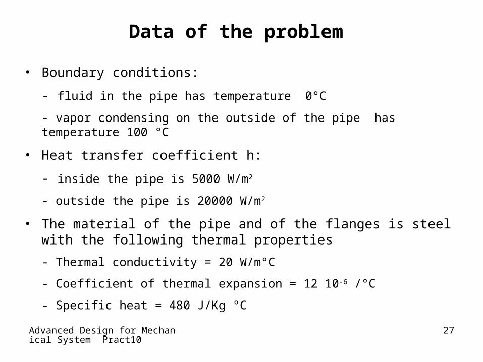
Data of the problem

• Boundary conditions:

- fluid in the pipe has temperature 0°C

- vapor condensing on the outside of the pipe has temperature 100 °C

• Heat transfer coefficient h:

- inside the pipe is 5000 W/m2

- outside the pipe is 20000 W/m2

• The material of the pipe and of the flanges is steel with the following thermal properties

- Thermal conductivity = 20 W/m°C

- Coefficient of thermal expansion = 12 10-6 /°C

- Specific heat = 480 J/Kg °C


28

Preliminary Analysis

• The maximum possible value of flux through the pipe wall is approximated by regarding the wall as plane and using the limiting surface temperature

• This is a maximum value because:

- the inside of the pipe must be warmer than 0°C

- the outside of the pipe must be cooler than 100 °C

2lim /286000

077.0084.0

010020 mW

r

Tkf


29

Axis of revolution

Model

Radial

Plane of symmetry

Plane of symmetry

Axisymmetric solid of revolution

Gap


30

Boundary conditions

• Between the welds, along IJ, pipe and flanges touch only at random and isolated point, if at all.

• Conductivity across this cylindrical surface is very low compared with solid metal and can be assumed equal zero

• This is a pessimistic assumption for eventual stress analysis, because it increase the thermal gradient and therefore increase stresses.


31

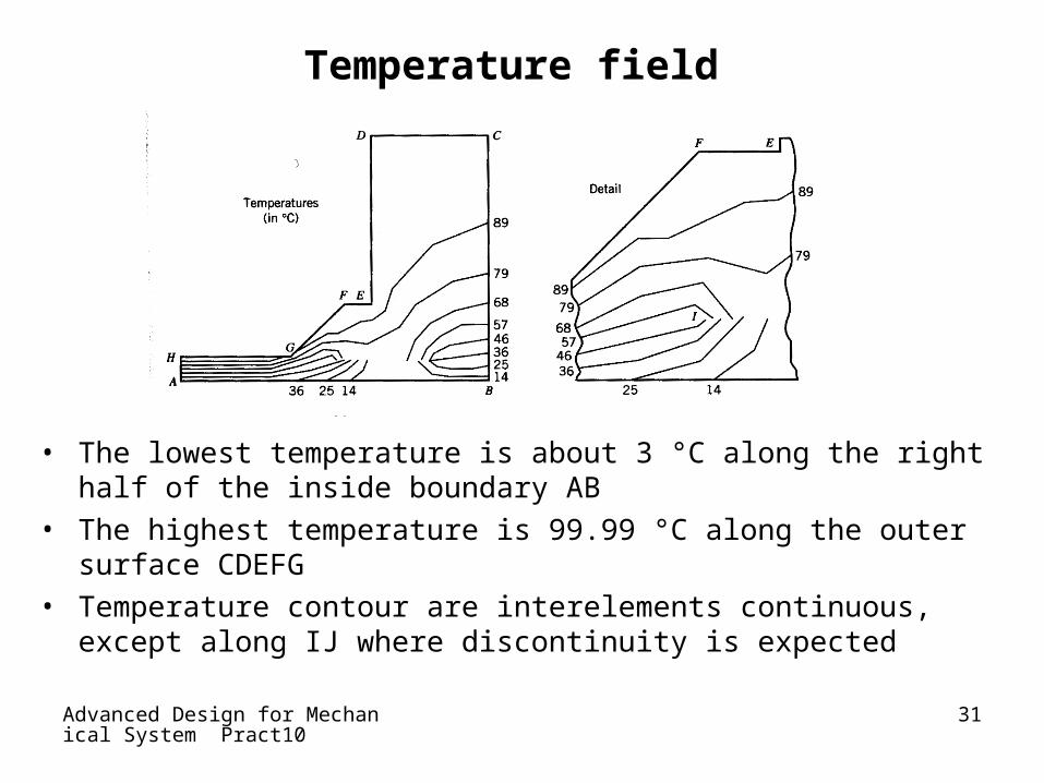
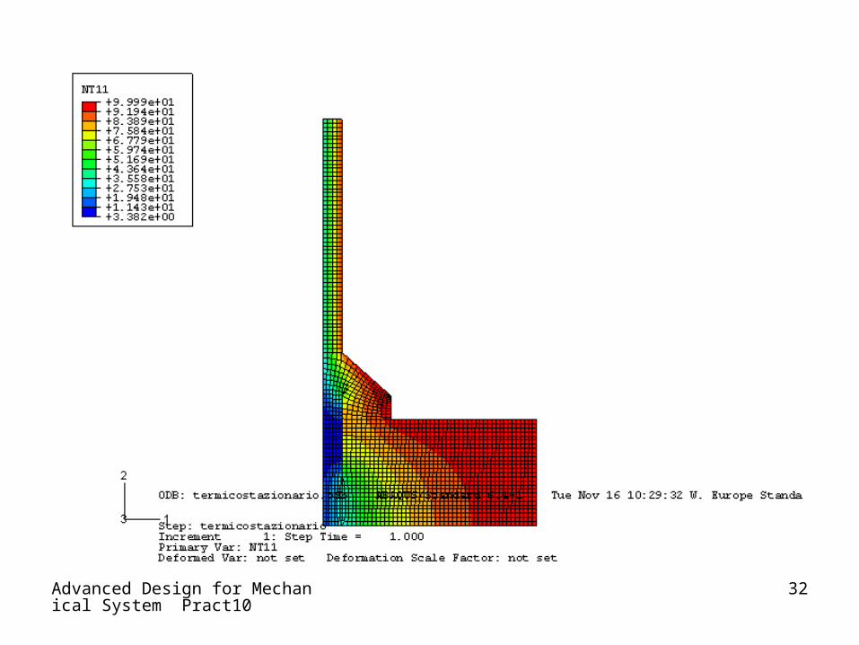
Temperature field

• The lowest temperature is about 3 °C along the right half of the inside boundary AB

• The highest temperature is 99.99 °C along the outer surface CDEFG• Temperature contour are interelements continuous, except along IJ

where discontinuity is expected


32


33

Thermal flux

• Flux arrows are perpendicular to the temperature contour because the material is isotropic

• Flux arrows agree with the expectation of preliminary analysis• Radial flux near AB is 170.000 W/m2 which, as expected is less that the

approximate limiting value.


34

Flux contour


35

Thermal transient


36

Thermomechanical analysis• The mesh used for the thermal analysis is used again, now with

computed nodal temperatures used to load the model.

• Two significant question about boundary arise:

- should nodes along BC be fixed against axial motion or not? Allowing movement gives no credit to resistance offered by the gasket and the bolts, while fixity gives too much credit.

We elect to run the stress analysis twice, first allowing motion along BC and second preventing it.

- is it proper to let nodes along IJ move independently?

If sides of the interface move apart, as the results shows, the answer is yes.


37

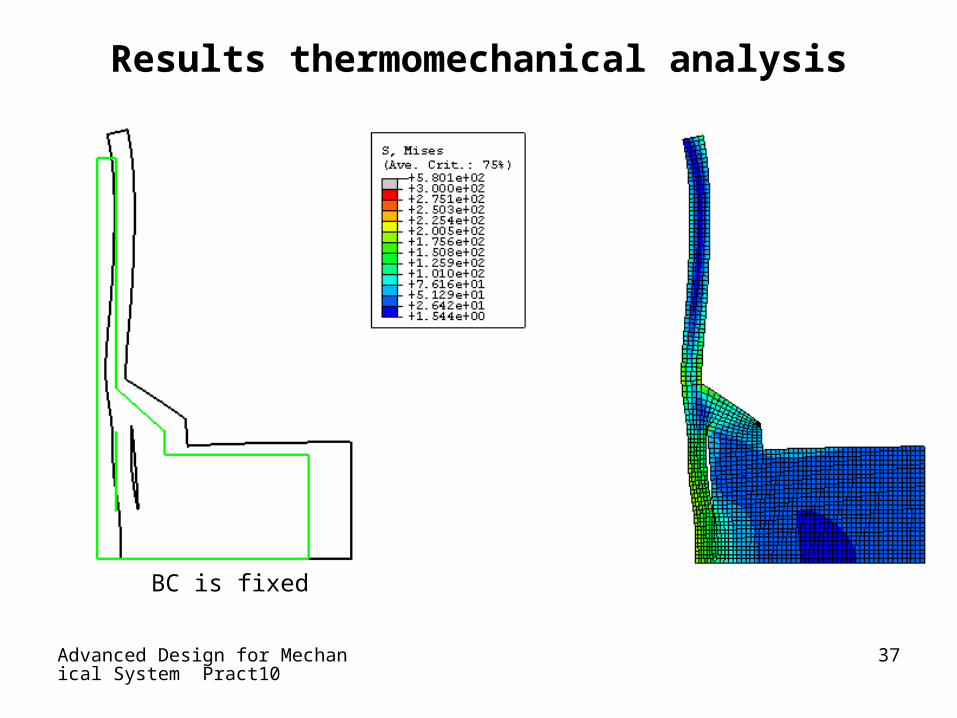
Results thermomechanical analysis

BC is fixed


38

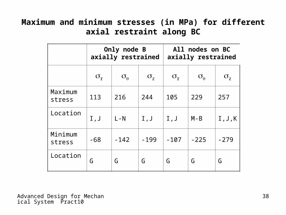
Maximum and minimum stresses (in MPa) for different axial restraint along BC

Only node B axially restrained

All nodes on BC axially restrained

r z r z

Maximum stress 113 216 244 105 229 257

LocationI,J L-N I,J I,J M-B I,J,K

Minimum stress -68 -142 -199 -107 -225 -279

LocationG G G G G G

Advanced Design for Mechanical System Pract10 1 Thermal analysis There is a resemblance between the...

Documents

Transcript of Advanced Design for Mechanical System Pract10 1 Thermal analysis There is a resemblance between the...