Advanced Data Structures for Games and Graphics Lecture 4 Advanced Programming for 3D Applications.
74
Advanced Data Structures Advanced Data Structures for Games and Graphics for Games and Graphics Lecture 4 Lecture 4 Advanced Programming for 3D Advanced Programming for 3D Applications Applications
-
date post
20-Dec-2015 -
Category
Documents
-
view
232 -
download
0
Transcript of Advanced Data Structures for Games and Graphics Lecture 4 Advanced Programming for 3D Applications.

Advanced Data StructuresAdvanced Data Structuresfor Games and Graphics for Games and Graphics
Lecture 4Lecture 4
Advanced Programming for 3D ApplicationsAdvanced Programming for 3D Applications
22
OverviewOverview
• Spatial Data StructuresSpatial Data Structures– Why care?Why care?– Octrees/QuadtreesOctrees/Quadtrees– Operations on tree-based spatial data structuresOperations on tree-based spatial data structures
• Kd-treesKd-trees• BSP treesBSP trees• BVHs (Bounding Volume Hierarchies)BVHs (Bounding Volume Hierarchies)• Cell Structures (Graph-Based)Cell Structures (Graph-Based)• VisibilityVisibility
– Portal basedPortal based– Occlusion cullingOcclusion culling

33
Spatial Data StructuresSpatial Data Structures
• Used to organize geometry in n-dimensional Used to organize geometry in n-dimensional space (2 and 3D) space (2 and 3D)
• For accelerating queries – culling, ray tracing For accelerating queries – culling, ray tracing intersection tests, collision detection intersection tests, collision detection
• They are mostly hierarchy (Tree-Based) by They are mostly hierarchy (Tree-Based) by naturenature
• Examples: Examples: – Bounding Volume Hierarchies (BVH)Bounding Volume Hierarchies (BVH)– Binary Space Partitioning Trees (BSP trees)Binary Space Partitioning Trees (BSP trees)– Octrees Octrees

44
Spatial Data StructuresSpatial Data Structures
• Spatial data structures store data indexed in Spatial data structures store data indexed in some way by their spatial locationsome way by their spatial location– For instance, store points according to their location, or For instance, store points according to their location, or
polygons, …polygons, …
• Multitude of uses in computer gamesMultitude of uses in computer games– Visibility - What can I see?Visibility - What can I see?– Ray intersections - What did the player just shoot?Ray intersections - What did the player just shoot?– Collision detection - Did the player just hit a wall?Collision detection - Did the player just hit a wall?– Proximity queries - Where is the nearest power-up?Proximity queries - Where is the nearest power-up?

55
Spatial DecompositionsSpatial Decompositions
• Focus on spatial data structures that partition Focus on spatial data structures that partition space into regions, or space into regions, or cellscells, of some type, of some type– Generally, cut up space with planes that separate Generally, cut up space with planes that separate
regionsregions– Almost always based on tree structuresAlmost always based on tree structures
• Octrees (Quadtrees)Octrees (Quadtrees): Axis aligned, regularly : Axis aligned, regularly spaced planes cut space into cubes (squares)spaced planes cut space into cubes (squares)
• Kd-treesKd-trees: Axis aligned planes, in alternating : Axis aligned planes, in alternating directions, cut space into rectilinear regionsdirections, cut space into rectilinear regions
• BSP TreesBSP Trees: Arbitrarily aligned planes cut space : Arbitrarily aligned planes cut space into convex regions into convex regions

66
OctreesOctrees
• Similar to Axis-Aligned BSP treesSimilar to Axis-Aligned BSP trees
• Each node has eight childrenEach node has eight children
• A parent has 8 (2x2x2) children
• Subdivide the space until the number of primitives within each leaf node is less than a threshold
• Objects are stored in the leaf nodes

77
OctreeOctree• Root node represents a cube containing the Root node represents a cube containing the
entire worldentire world• Then, recursively, the eight children of each Then, recursively, the eight children of each
node represent the eight sub-cubes of the node represent the eight sub-cubes of the parentparent
• Objects can be assigned to nodes in one of two Objects can be assigned to nodes in one of two common ways:common ways:– All objects are in leaf nodesAll objects are in leaf nodes– Each object is in the smallest node that fully contains Each object is in the smallest node that fully contains
itit– What are the benefits and problems with each What are the benefits and problems with each
approach?approach?

88
Octree Node Data Octree Node Data StructureStructure• What needs to be stored in a node?What needs to be stored in a node?
– Children pointers (at most eight)Children pointers (at most eight)– Parent pointer - useful for moving about the treeParent pointer - useful for moving about the tree– Extents of cube - can be inferred from tree structure, Extents of cube - can be inferred from tree structure,
but easier to just store itbut easier to just store it– Data associated with the contents of the cubeData associated with the contents of the cube
• Contents might be whole objects or individual polygons, Contents might be whole objects or individual polygons, or even something elseor even something else
– Neighbors are useful in some algorithmsNeighbors are useful in some algorithms

99
Building an OctreeBuilding an Octree
• Define a function, Define a function, buildNodebuildNode, that:, that:– Takes a node with its cube and set a list of Takes a node with its cube and set a list of
its contentsits contents– Creates the children nodes, divides the Creates the children nodes, divides the
objects among the children, and recurses on objects among the children, and recurses on the children, orthe children, or
– Sets the node to be a leaf nodeSets the node to be a leaf node• Find the root cube, create the root node Find the root cube, create the root node
and call and call buildNodebuildNode with all the objects with all the objects• When do we choose to stop creating When do we choose to stop creating
children?children?

1010
Example ConstructionExample Construction

1111
Frustum Culling With Frustum Culling With OctreesOctrees• We wish to eliminate objects that do not We wish to eliminate objects that do not
intersect the view frustumintersect the view frustum• Have a test that succeeds if a cell may be visibleHave a test that succeeds if a cell may be visible
– Test the corners of the cell against each clip plane. If all Test the corners of the cell against each clip plane. If all the corners are outside one clip plane, the cell is not the corners are outside one clip plane, the cell is not visiblevisible
– Otherwise, is the cell itself definitely visible?Otherwise, is the cell itself definitely visible?• Starting with the root node cell, perform the testStarting with the root node cell, perform the test
– If it fails, nothing inside the cell is visibleIf it fails, nothing inside the cell is visible– If it succeeds, something inside the cell might be visibleIf it succeeds, something inside the cell might be visible– Recurse for each of the children of a visible cellRecurse for each of the children of a visible cell
• This algorithm with quadtrees is particularly This algorithm with quadtrees is particularly effective for certain type of game. effective for certain type of game.

1212
Visibility Culling Visibility Culling
• Back face culling Back face culling
• View-frustrum culling View-frustrum culling
• Detail culling Detail culling
• Occlusion culling Occlusion culling

1313
View-Frustum CullingView-Frustum Culling
• Done in the application stage Done in the application stage
• Remove objects that are outside Remove objects that are outside the viewing frustumthe viewing frustum
• Can use BVH, BSP, OctreesCan use BVH, BSP, Octrees
1. Create hierarchy2. BV/V-F intersection tests

1414
View-Frustum CullingView-Frustum Culling
• Often done hierarchically to save Often done hierarchically to save time time
In-order, top-downtraversal and test
1515
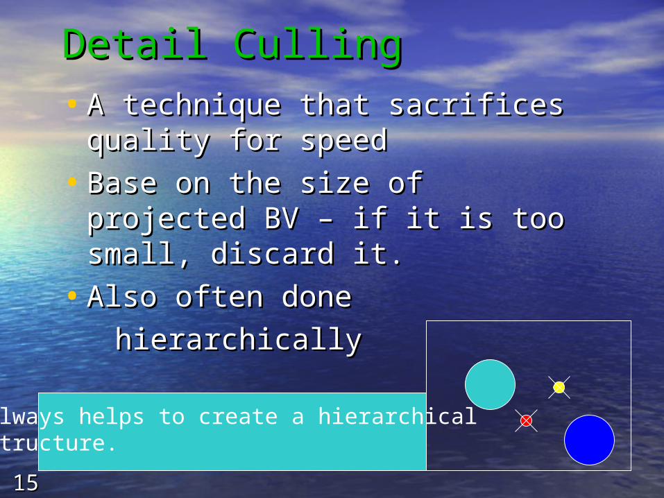
Detail Culling Detail Culling • A technique that sacrifices A technique that sacrifices
quality for speedquality for speed
• Base on the size of projected BV Base on the size of projected BV – if it is too small, discard it.– if it is too small, discard it.
• Also often done Also often done
hierarchically hierarchically
Always helps to create a hierarchical structure.

1616
Occlusion CullingOcclusion Culling
• Discard objects that are occludedDiscard objects that are occluded
• Z-buffer is not the smartest algorithm in Z-buffer is not the smartest algorithm in the world (particularly for high depth-the world (particularly for high depth-
complexity scenes)complexity scenes)
• We want to avoid processing invisible We want to avoid processing invisible objectsobjects
• Combine Spatial Data Structure and Z-Combine Spatial Data Structure and Z-BufferBuffer

1717
Occlusion Culling (2)Occlusion Culling (2)
OcclusionCulling (G) Or = empty For each object g in G if (isOccluded(g, Or))
skip g else
render (g) update (Or) end End
G: input graphics dataOr: occlusion hint
Things needed: 1. Algorithms for isOccluded()2. What is Or? 3. Fast update Or

1818
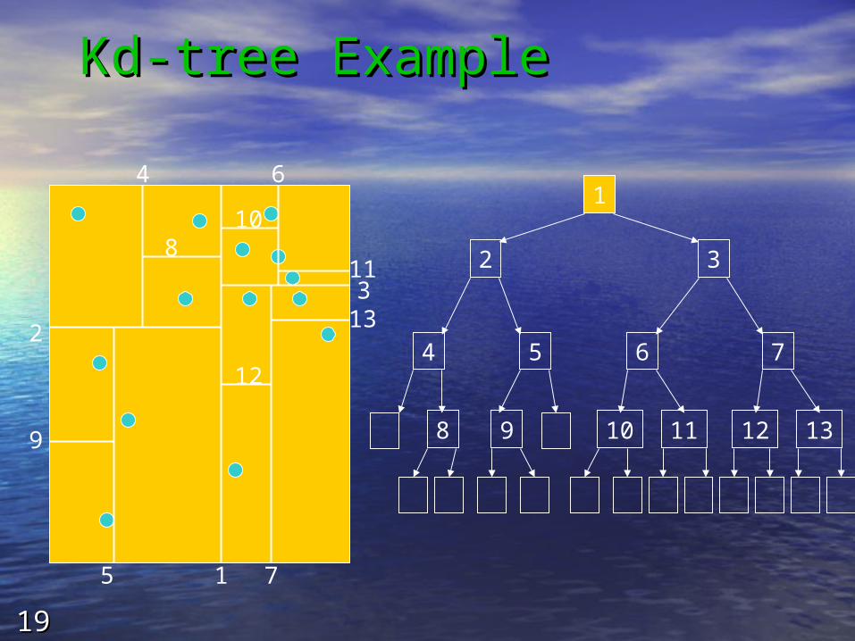
Kd-treesKd-trees• A kd-tree is a tree with the following propertiesA kd-tree is a tree with the following properties
– Each node represents a rectilinear region (faces aligned with Each node represents a rectilinear region (faces aligned with axes)axes)
– Each node is associated with an axis aligned plane that cuts Each node is associated with an axis aligned plane that cuts its region into two, and it has a child for each sub-regionits region into two, and it has a child for each sub-region
– The directions of the cutting planes alternate with depth – The directions of the cutting planes alternate with depth – height 0 cuts on x, height 1 cuts on height 0 cuts on x, height 1 cuts on yy, height 2 cuts on , height 2 cuts on zz, , height 3 cuts on height 3 cuts on xx, …, …
• Kd-trees generalize octrees by allowing splitting Kd-trees generalize octrees by allowing splitting planes at variable positionsplanes at variable positions– Note that cut planes in different sub-trees at the same level Note that cut planes in different sub-trees at the same level
need not be the sameneed not be the same
1919
Kd-tree ExampleKd-tree Example
1
1
2 3
2
3
4 5 6 7
4
5
6
7
8 9 10 11 12 13
8
9
10
11
12
13

2020
Kd-tree ExampleKd-tree Example
1
1
2 3
2
3
4 5 6 7
4
5
6
7
8 9 10 11 12 13
8
9
10
11
12
13

2121
Kd-tree ExampleKd-tree Example
1
1
2 3
2
3
4 5 6 7
4
5
6
7
8 9 10 11 12 13
8
9
10
11
12
13

2222
Kd-tree Node Data Kd-tree Node Data StructureStructure• What needs to be stored in a What needs to be stored in a
node?node?– Children pointers (always two)Children pointers (always two)– Parent pointer - useful for moving about the Parent pointer - useful for moving about the
treetree
– Extents of cell - xExtents of cell - xmaxmax, x, xminmin, y, ymaxmax, y, yminmin, z, zmaxmax, z, zminmin
– List of pointers to the contents of the cellList of pointers to the contents of the cell– Neighbors are complicated in kd-trees, so Neighbors are complicated in kd-trees, so
typically not storedtypically not stored

2323
Building a Kd-treeBuilding a Kd-tree
• Define a function, Define a function, buildNodebuildNode, that:, that:– Takes a node with its cell defined and a list of its Takes a node with its cell defined and a list of its
contentscontents– Sets the splitting plane, creates the children nodes, Sets the splitting plane, creates the children nodes,
divides the objects among the children, and recurses divides the objects among the children, and recurses on the children, oron the children, or
– Sets the node to be a leaf nodeSets the node to be a leaf node
• Find the root cell, create the root node and call Find the root cell, create the root node and call buildNodebuildNode with all the objects with all the objects
• When do we choose to stop creating children?When do we choose to stop creating children?

2424
Choosing a Splitting PlaneChoosing a Splitting Plane• Two common goals in selecting a splitting plane for Two common goals in selecting a splitting plane for
each celleach cell– Minimize the number of objects cut by the planeMinimize the number of objects cut by the plane– Balance the tree: Use the plane that equally divides the Balance the tree: Use the plane that equally divides the
objects into two sets (the objects into two sets (the median cutmedian cut plane) plane)– One possible global goal is to minimize the number of One possible global goal is to minimize the number of
objects cut throughout the entire tree objects cut throughout the entire tree
• One method (assuming splitting on plane One method (assuming splitting on plane perpendicular to x-axis):perpendicular to x-axis):– Sort all the vertices of all the objects to be stored according Sort all the vertices of all the objects to be stored according
to xto x– Put plane through median vertex, or locally search for low Put plane through median vertex, or locally search for low
cut planecut plane

2525
BSP TreesBSP Trees• Binary Space PartitionBinary Space Partition trees trees
– A sequence of cuts that divide a region of space into A sequence of cuts that divide a region of space into twotwo
• Cutting planes can be of any orientationCutting planes can be of any orientation– A generalization of kd-trees, and sometimes a kd-tree A generalization of kd-trees, and sometimes a kd-tree
is called an axis-aligned BSP treeis called an axis-aligned BSP tree
• Divides space into convex cellsDivides space into convex cells• The industry standard for spatial subdivision in The industry standard for spatial subdivision in
game environmentsgame environments– General enough to handle most common environmentsGeneral enough to handle most common environments– Easy enough to manage and understandEasy enough to manage and understand– Big performance gainsBig performance gains

2626
Binary Space Partitioning Binary Space Partitioning (BSP) Trees(BSP) Trees• Main purpose – depth sorting Main purpose – depth sorting
• Consisting of a dividing plane, and a BSP Consisting of a dividing plane, and a BSP tree on each side of the dividing plane tree on each side of the dividing plane (note the recursive definition)(note the recursive definition)
• The back to front traversal order can be The back to front traversal order can be decided right away according to where the decided right away according to where the eye is eye is
BSP A
BSP B
P back to front: A->P->B
back to front: A->P->B

2727
BSP Trees (cont’d) BSP Trees (cont’d)
• Two possible implementations: Two possible implementations:
Axis-Aligned BSP Polygon-Aligned BSP

2828
Axis-Aligned BSP Trees Axis-Aligned BSP Trees • Starting with an AABB Starting with an AABB
• Recursively subdivide into small boxes Recursively subdivide into small boxes
• One possible strategy: cycle through the One possible strategy: cycle through the axes (also called axes (also called k-d treesk-d trees) )
A
B
C
D E
0
1a1b
2
0
1a 1b
A B C 2
D E

2929
Polygon-Aligned BSP TreesPolygon-Aligned BSP Trees• The original BSP idea The original BSP idea
• Choose one divider at a time – any polygon Choose one divider at a time – any polygon intersect with the plane has to be split intersect with the plane has to be split
• Done recursively until all polygons are in the BSP Done recursively until all polygons are in the BSP trees trees
• The back to front traversal can be done exact The back to front traversal can be done exact
• The dividers need to be chosen carefully so that a The dividers need to be chosen carefully so that a balanced BSP tree is created balanced BSP tree is created
A
B
F
DE
result of split
C
A
B
D E
C
F

3030
BSP ExampleBSP Example
• Notes:Notes:– Splitting planes end when they Splitting planes end when they
intersect their parent node’s planesintersect their parent node’s planes– Internal node labeled with planes, leaf Internal node labeled with planes, leaf
nodes with regionsnodes with regions
1
42
3 75
BA out8
D out
6
C out
12
3
4
56
78
outA
outBC
D

3131
BSP Tree Node Data BSP Tree Node Data StructureStructure• What needs to be stored in a node?What needs to be stored in a node?
– Children pointers (always two)Children pointers (always two)– Parent pointer - useful for moving about the treeParent pointer - useful for moving about the tree– If a leaf node: Extents of cellIf a leaf node: Extents of cell
• How might we store it?How might we store it?
– If an internal node: The split planeIf an internal node: The split plane– List of pointers to the contents of the cellList of pointers to the contents of the cell– Neighbors are useful in many algorithmsNeighbors are useful in many algorithms
• Typically only store neighbors at leaf nodesTypically only store neighbors at leaf nodes
• Cells can have many neighboring cellsCells can have many neighboring cells
– Portals are also useful - holes that see into neighborsPortals are also useful - holes that see into neighbors

3232
Building a BSP TreeBuilding a BSP Tree• Define a function, buildNode, that:Define a function, buildNode, that:
– Takes a node with its cell defined and a list of its Takes a node with its cell defined and a list of its contentscontents
– Sets the splitting plane, creates the children nodes, Sets the splitting plane, creates the children nodes, divides the objects among the children, and recurses divides the objects among the children, and recurses on the children, oron the children, or
– Sets the node to be a leaf nodeSets the node to be a leaf node
• Create the root node and call buildNode with all Create the root node and call buildNode with all the objectsthe objects– Do we need the root node’s cell? What do we set it to?Do we need the root node’s cell? What do we set it to?
• When do we choose to stop creating children?When do we choose to stop creating children?

3333
Choosing Splitting PlanesChoosing Splitting Planes• Goals:Goals:
– Trees with few cellsTrees with few cells– Planes that are mostly opaque (best for visibility Planes that are mostly opaque (best for visibility
calculations)calculations)– Objects not split across cellsObjects not split across cells
• Some heuristics:Some heuristics:– Choose planes that are also polygon planesChoose planes that are also polygon planes– Choose large polygons firstChoose large polygons first– Choose planes that don’t split many polygonsChoose planes that don’t split many polygons– Try to choose planes that evenly divide the dataTry to choose planes that evenly divide the data– Let the user select or otherwise guide the splitting Let the user select or otherwise guide the splitting
processprocess– Random choice of splitting planes doesn’t do too Random choice of splitting planes doesn’t do too
badlybadly

3434
BSP in Current GamesBSP in Current Games• Use a BSP tree to partition space as you would Use a BSP tree to partition space as you would
with an octree or kd-treewith an octree or kd-tree– Leaf nodes are cells with lists of objectsLeaf nodes are cells with lists of objects– Cells typically roughly correspond to “rooms”, but Cells typically roughly correspond to “rooms”, but
don’t have todon’t have to• The polygons to use in the partitioning are The polygons to use in the partitioning are
defined by the level designer as they build the defined by the level designer as they build the spacespace

3535
Bounding Volume Bounding Volume HierarchiesHierarchies• So far, we have had subdivisions that break the world So far, we have had subdivisions that break the world
into cellinto cell
• General General Bounding Volume HierarchiesBounding Volume Hierarchies (BVHs) start with (BVHs) start with a bounding volume for each objecta bounding volume for each object– Many possibilities: Spheres, AABBs, OBBs,…Many possibilities: Spheres, AABBs, OBBs,…
• Parents have a bound that bounds their children’s Parents have a bound that bounds their children’s boundsbounds– Typically, parent’s bound is of the same type as the Typically, parent’s bound is of the same type as the
children’schildren’s– Can use fixed or variable number of children per Can use fixed or variable number of children per
nodenode
• No notion of cells in this structureNo notion of cells in this structure

3636
Bounding Volume Bounding Volume HierarchiesHierarchies• Bounding Volume (BV) – a volume that encloses a set of Bounding Volume (BV) – a volume that encloses a set of
objects objects • The idea is to use a much similar geometric shape for The idea is to use a much similar geometric shape for
quick tests (frustum culling for example)quick tests (frustum culling for example)• Easy to compute, as tight as possibleEasy to compute, as tight as possible
• AABB, Sphere – easy to compute, but poor fitAABB, Sphere – easy to compute, but poor fitAABB Sphere OBB

3737
Bounding Volume Bounding Volume HierarchiesHierarchies• Each node has a bounding volume that Each node has a bounding volume that
encloses the geometry in the entire encloses the geometry in the entire subtreesubtree
• The actual geometry is contained in the The actual geometry is contained in the leaf node leaf node
• Three types of methods: bottom-up, Three types of methods: bottom-up, insertion, and top-downinsertion, and top-down
root
leaves

3838
BVH ExampleBVH Example

3939
BVH ConstructionBVH Construction• Simplest to build top-downSimplest to build top-down
– Bound everythingBound everything– Choose a split plane (or more), divide objects into setsChoose a split plane (or more), divide objects into sets– Recurse on child setsRecurse on child sets
• Can also be built incrementallyCan also be built incrementally– Insert one bound at a time, growing as requiredInsert one bound at a time, growing as required– Good for environments where things are created Good for environments where things are created
dynamicallydynamically
• Can also build bottom upCan also build bottom up– Bound individual objects, group them into sets, create Bound individual objects, group them into sets, create
parent, recurseparent, recurse– What’s the hardest part about this?What’s the hardest part about this?

4040
BVH OperationsBVH Operations
• Some of the operations we’ve mentionned work Some of the operations we’ve mentionned work with BVHswith BVHs– Frustum cullingFrustum culling– Collision detectionCollision detection
• BVHs are good for moving objectsBVHs are good for moving objects– Updating the tree is easier than for other Updating the tree is easier than for other
methodsmethods– Incremental construction also helps (don’t need Incremental construction also helps (don’t need
to rebuild the whole tree if something changes)to rebuild the whole tree if something changes)• But, BVHs lack some convenient propertiesBut, BVHs lack some convenient properties
– For example, not all space is filled, so For example, not all space is filled, so algorithms that “walk” through cells won’t workalgorithms that “walk” through cells won’t work

4141
Hierarchical Visibility Hierarchical Visibility
• One example of occlusion culling One example of occlusion culling techniquestechniques
• Object-space octreeObject-space octree– Primitives in an octree node are hidden Primitives in an octree node are hidden
if the octree node (cube) is hiddenif the octree node (cube) is hidden– A octree cube is hidden if its 6 faces A octree cube is hidden if its 6 faces
are hidden polygons are hidden polygons – Hierarchical visibility test: Hierarchical visibility test:

4242
Hierarchical VisibilityHierarchical Visibility
From the root of octree: From the root of octree: • View-frustum culling View-frustum culling • Scan conversion each of the 6 faces and Scan conversion each of the 6 faces and
perform z-buffering perform z-buffering • If all 6 faces are hidden, discard the entire If all 6 faces are hidden, discard the entire
node and sub-branchesnode and sub-branches• Otherwise, render the primitives inside and Otherwise, render the primitives inside and
traverse the front-to-back children recursivelytraverse the front-to-back children recursively
A conservative algorithm –
4343
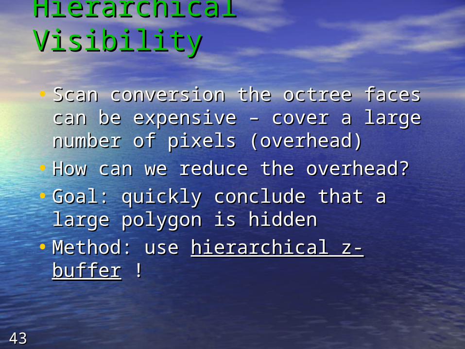
• Scan conversion the octree faces Scan conversion the octree faces can be expensive – cover a large can be expensive – cover a large number of pixels (overhead)number of pixels (overhead)
• How can we reduce the overhead? How can we reduce the overhead?
• Goal: quickly conclude that a large Goal: quickly conclude that a large polygon is hiddenpolygon is hidden
• Method: use Method: use hierarchical z-bufferhierarchical z-buffer ! !
Hierarchical VisibilityHierarchical Visibility
4444
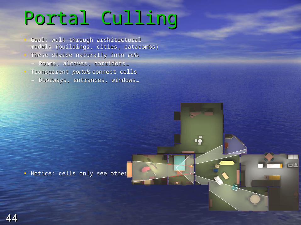
Portal Culling Portal Culling • Goal: walk through architectural Goal: walk through architectural
models (buildings, cities, catacombs)models (buildings, cities, catacombs)
• These divide naturally into These divide naturally into cellscells– Rooms, alcoves, corridors… Rooms, alcoves, corridors…
• Transparent Transparent portals portals connect cellsconnect cells– Doorways, entrances, windows… Doorways, entrances, windows…
• Notice: cells only see other cells through portalsNotice: cells only see other cells through portals

4545
PortalsPortals
• Subdivision of the world Subdivision of the world into into cellscells and and portalsportals
• Any region of space that Any region of space that cannot be seen through a cannot be seen through a sequence of portals is sequence of portals is never considered for never considered for renderingrendering
• Culling cells seen through Culling cells seen through a portal is done using a a portal is done using a frustum reduced in size frustum reduced in size by the portal boundaryby the portal boundary

4646
Cells & PortalsCells & Portals
• An example:An example:

4747
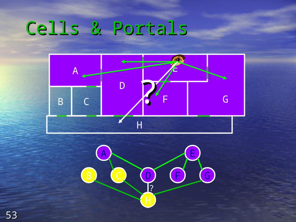
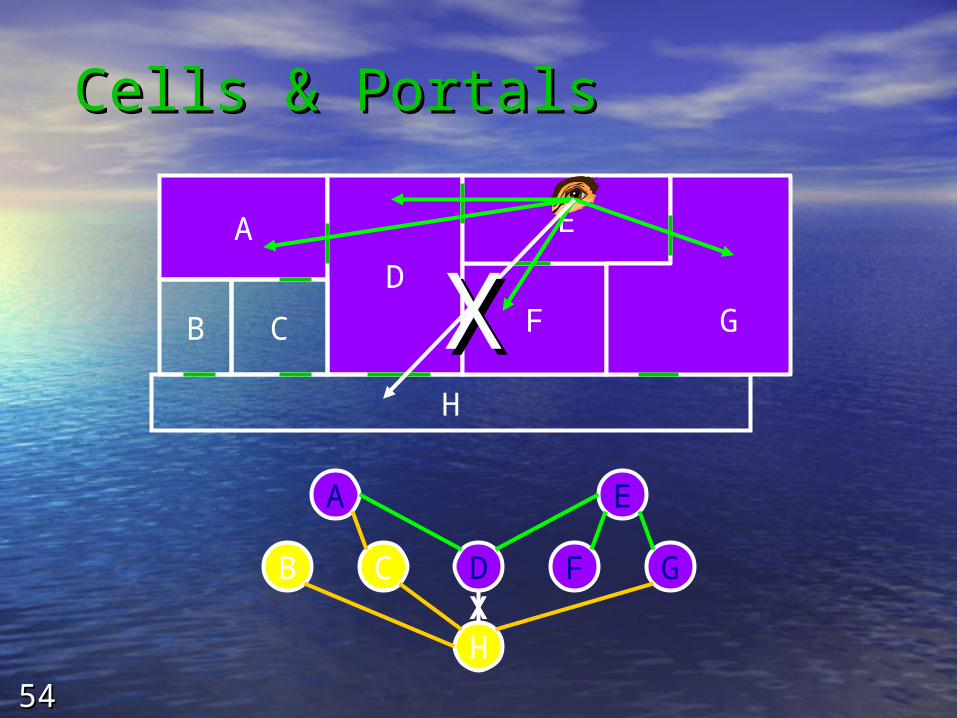
Cells & PortalsCells & Portals
• Idea: Idea: – Create an Create an adjacency graph adjacency graph of cellsof cells– Starting with cell containing eyepoint, Starting with cell containing eyepoint,
traverse graph, rendering visible cells traverse graph, rendering visible cells – A cell is only visible if it can be seen A cell is only visible if it can be seen
through a sequence of portalsthrough a sequence of portals• So cell visibility reduces to testing portal So cell visibility reduces to testing portal
sequences for a sequences for a line of sight…line of sight…

4848
Cells & PortalsCells & Portals
A
D
H
FCB
E
G
H
B C D F G
EA

4949
Cells & PortalsCells & Portals
A
D
H
FCB
E
G
H
B C D F G
EA

5050
Cells & PortalsCells & Portals
A
D
H
FCB
E
G
H
B C D F G
EA

5151
Cells & PortalsCells & Portals
A
D
H
FCB
E
G
H
B C D F G
EA

5252
Cells & PortalsCells & Portals
A
D
H
FCB
E
G
H
B C D F G
EA
5353
Cells & PortalsCells & Portals
A
D
H
FCB
E
G
H
B C D F G
EA
?
??
5454
Cells & PortalsCells & Portals
A
D
H
FCB
E
G
H
B C D F G
EA
X
XX

5555
Cells & PortalsCells & Portals
• View-independentView-independent solution: find all cells a particular solution: find all cells a particular cell could cell could possiblypossibly see: see:
C can C can onlyonly see A, D, E, and H see A, D, E, and H
A
D
H
FCB
E
G
A
D
H
E

5656
Cells & PortalsCells & Portals
• View-independentView-independent solution: find all cells a particular solution: find all cells a particular cell could cell could possiblypossibly see: see:
H will H will nevernever see F see F
A
D
H
FCB
E
G
A
D
CB
E
G

5757
Portal DefinitionsPortal Definitions
• A A cellcell is a region of space is a region of space
• A A portalportal is a transparent region that is a transparent region that connects cellsconnects cells– Portals are one-way (front faced)Portals are one-way (front faced)
• A portal is represented by a A portal is represented by a convex convex planarplanar polygon polygon
• Information on cells and the portals Information on cells and the portals connecting them are stored in an connecting them are stored in an adjacency graphadjacency graph

5858
Portal RenderingPortal Rendering1.1. Initialize the current frustum to the entire Initialize the current frustum to the entire
view frustumview frustum2.2. Set the active cell to be the cell in which the Set the active cell to be the cell in which the
camera resides and draw this cellcamera resides and draw this cell3.3. For each visible portal in the currently active For each visible portal in the currently active
cell do:cell do:1.1. Find the reduced view frustum due to the portalFind the reduced view frustum due to the portal2.2. Recursively draw the cell at the other side of the Recursively draw the cell at the other side of the
portal, using the reduced view frustumportal, using the reduced view frustum
A
D
H
FCB
E
G

5959
Cell-Portal StructuresCell-Portal Structures
• Cell-Portal data structures dispense with the Cell-Portal data structures dispense with the hierarchy and just store neighbor informationhierarchy and just store neighbor information– This make them graphs, not treesThis make them graphs, not trees
• Cells are described by bounding polygonsCells are described by bounding polygons• Portals are polygonal openings between cellsPortals are polygonal openings between cells• Good for visibility culling algorithms, OK for Good for visibility culling algorithms, OK for
collision detection and ray-castingcollision detection and ray-casting• Several ways to constructSeveral ways to construct
– By hand, as part of an authoring processBy hand, as part of an authoring process– Automatically, starting with a BSP tree or kd-tree and Automatically, starting with a BSP tree or kd-tree and
extracting cells and portalsextracting cells and portals– Explicitly, as part of an automated modeling processExplicitly, as part of an automated modeling process

6060
Cell-Portal VisibilityCell-Portal Visibility
• Keep track of which cell the viewer is inKeep track of which cell the viewer is in
• Somehow walk the graph to enumerate Somehow walk the graph to enumerate all the visible regionsall the visible regions
• Cell-based: Preprocess to identify the Cell-based: Preprocess to identify the potentially visible set (PVS) for each cellpotentially visible set (PVS) for each cell– Set may contain whole cells or Set may contain whole cells or
individual objectsindividual objects
• Point-based: Traverse the graph at Point-based: Traverse the graph at runtimeruntime– Granularity can be whole cells, Granularity can be whole cells,
regions, or objectsregions, or objects
• Trend is toward point-based, but cell-Trend is toward point-based, but cell-based is still very commonbased is still very common

6161
Runtime Portal VisibilityRuntime Portal Visibility• Define a procedure Define a procedure renderCellrenderCell::
– Takes a view frustum and a cellTakes a view frustum and a cell• Viewer not necessarily in the cellViewer not necessarily in the cell
– Draws the contents of the cell that are in the frustumDraws the contents of the cell that are in the frustum– For each portal out of the cell, clips the frustum to that For each portal out of the cell, clips the frustum to that
portal and recurses with the new frustum and the cell portal and recurses with the new frustum and the cell beyond the portalbeyond the portal• Make sure not to go to the cell you enteredMake sure not to go to the cell you entered
• Start in the cell containing the viewer, with the full Start in the cell containing the viewer, with the full viewing frustumviewing frustum
• Stop when no more portals intersect the view Stop when no more portals intersect the view frustumfrustum

6262
Potentially Visible SetsPotentially Visible Sets
• A Potentially Visible Set (PVS) is an array A Potentially Visible Set (PVS) is an array stored for each cell holding the visibility stored for each cell holding the visibility information of all other cells from that cellinformation of all other cells from that cell
• If cell A is not listed in cell Bs PVS, it cannot If cell A is not listed in cell Bs PVS, it cannot possibly be visible from inside cell B, and possibly be visible from inside cell B, and therefore doesn’t need to be considered for therefore doesn’t need to be considered for renderedrendered
• Unlike basic portal rendering, the cells used for Unlike basic portal rendering, the cells used for PVS calculations must be convex regionsPVS calculations must be convex regions
6363
Potentially Visible SetsPotentially Visible Sets
• PVS: The set of cells/regions/objects/polygons that can PVS: The set of cells/regions/objects/polygons that can be seen from a particular cellbe seen from a particular cell– Generally, choose to identify objects that can be Generally, choose to identify objects that can be
seenseen– Trade-off is memory consumption vs. accurate Trade-off is memory consumption vs. accurate
visibilityvisibility• Computed as a pre-processComputed as a pre-process
– Have to have a strategy to manage dynamic objectsHave to have a strategy to manage dynamic objects• Used in various ways:Used in various ways:
– As the only visibility computation - render everything As the only visibility computation - render everything in the PVS for the viewer’s current cellin the PVS for the viewer’s current cell
– As a first step - identify regions that are of interest As a first step - identify regions that are of interest for more accurate run-time algorithmsfor more accurate run-time algorithms

6464
Why not just Frustum Why not just Frustum Culling?Culling?• A PVS can be pre-A PVS can be pre-
calculated, thus at calculated, thus at runtime large runtime large portions of the scene portions of the scene can be culled without can be culled without any testing at allany testing at all
• A PVS can rule out A PVS can rule out cells that, although cells that, although inside the view inside the view frustum, cannot frustum, cannot possibly be visiblepossibly be visible

6565
Calculating the PVSCalculating the PVS• A cell A is potentially visible from cell B through a A cell A is potentially visible from cell B through a
portal sequence, if and only if there exists a portal sequence, if and only if there exists a straight line stabbing all portals in the sequencestraight line stabbing all portals in the sequence
• If a cell A is connected to cell B through a single If a cell A is connected to cell B through a single portal only, it is always part of cell Bs PVSportal only, it is always part of cell Bs PVS
• If a cell A is connected to cell B through a If a cell A is connected to cell B through a sequence of two portals, it is part of cell Bs PVS sequence of two portals, it is part of cell Bs PVS unless the two portals are coplanarunless the two portals are coplanar

6666
Cell-to-Cell PVSCell-to-Cell PVS• Cell A is in cell B’s PVS if there exist a Cell A is in cell B’s PVS if there exist a stabbing linestabbing line
that originates on a portal of B and reaches a that originates on a portal of B and reaches a portal of Aportal of A– A A stabbing linestabbing line is a line segment intersecting only portals is a line segment intersecting only portals– Neighbor cells are trivially in the PVSNeighbor cells are trivially in the PVS
I J
H
GA
CB E
F
D
PVS for I contains:B, C, E, F, H, J

6767
Direct Portal Rendering vs. Direct Portal Rendering vs. PVSPVS• Setup cost and preprocessing timeSetup cost and preprocessing time
– PVS calculation is a time consuming process, and is best done PVS calculation is a time consuming process, and is best done in a preprocessing step, however once it has been calculated, in a preprocessing step, however once it has been calculated, using it is practically for freeusing it is practically for free
– Direct portal rendering requires no preprocessing, however Direct portal rendering requires no preprocessing, however there is a run time cost as passing through a portal requires there is a run time cost as passing through a portal requires regenerating the viewing volumeregenerating the viewing volume
• Few or many portalsFew or many portals– PVS rendering is (nearly) unaffected by the number of portals PVS rendering is (nearly) unaffected by the number of portals
and cellsand cells– Because of the cost for passing a portal and regenerating the Because of the cost for passing a portal and regenerating the
viewing volume, direct portal rendering is best suited for viewing volume, direct portal rendering is best suited for scenes with a moderate number of portalsscenes with a moderate number of portals
• Automatic or manual portal placementAutomatic or manual portal placement– Currently, the only automatic portal placement algorithms Currently, the only automatic portal placement algorithms
produce a large number of portals. Automatic portal placement produce a large number of portals. Automatic portal placement is therefore currently only suited for PVS based systemsis therefore currently only suited for PVS based systems

6868
Direct Portal Rendering vs. Direct Portal Rendering vs. PVSPVS• Static or dynamic portalsStatic or dynamic portals
– As PVS calculations are slow, and moving a portal As PVS calculations are slow, and moving a portal requires recalculating the PVS, the portals in a requires recalculating the PVS, the portals in a PVS system must be staticPVS system must be static
– Direct portal rendering requires no pre-Direct portal rendering requires no pre-calculations, so a portal is free to move without calculations, so a portal is free to move without introducing a performance penaltyintroducing a performance penalty
• Underlying data structureUnderlying data structure– PVS rendering is well suited for leaf BSP trees, as PVS rendering is well suited for leaf BSP trees, as
the leafs are convex regions of space connected the leafs are convex regions of space connected through portalsthrough portals
– Direct portal rendering is not suitable for Direct portal rendering is not suitable for combination with leaf BSP trees due to the high combination with leaf BSP trees due to the high number of portals generated this waynumber of portals generated this way
6969
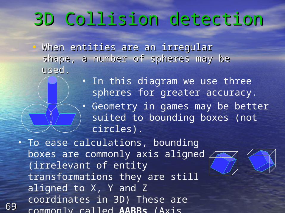
3D Collision detection3D Collision detection
• When entities are an irregular shape, a When entities are an irregular shape, a number of spheres may be used.number of spheres may be used.
• In this diagram we use three spheres for greater accuracy.
• Geometry in games may be better suited to bounding boxes (not circles).
• To ease calculations, bounding boxes are commonly axis aligned (irrelevant of entity transformations they are still aligned to X, Y and Z coordinates in 3D) These are commonly called AABBs (Axis Aligned Bounding Boxes).

7070
Recursive testing of Recursive testing of bounding boxesbounding boxes• We can build up a recursive hierarchy of bounding boxes We can build up a recursive hierarchy of bounding boxes
to determine quite accurate collision detection.to determine quite accurate collision detection.
• Here we use a sphere to test for course grain intersection.
• If we detect intersection of the sphere, we test the two sub bounding boxes.
• The lower bounding box is further reduced to two more bounding boxes to detect collision of the cylinders.

7171
Tree structure used to Tree structure used to model collision detectionmodel collision detection
• A recursive algorithm can be used to parse the tree structure A recursive algorithm can be used to parse the tree structure for detecting collisions.for detecting collisions.
• If a collision is detected and leaf nodes are not null then If a collision is detected and leaf nodes are not null then traverse the leaf nodes.traverse the leaf nodes.
• If a collision is detected and the leaf nodes are null then If a collision is detected and the leaf nodes are null then collision has occurred at the current node in the the structure.collision has occurred at the current node in the the structure.
• If no collision is detected at all nodes where leaf nodes are null If no collision is detected at all nodes where leaf nodes are null then no collision has occurred (in our diagram B, C or D must then no collision has occurred (in our diagram B, C or D must record collision).record collision).
A B
C
D
E
A
B C
D E

7272
Separating axisSeparating axis
• In 2D we can easily see if two AABBs overlap.In 2D we can easily see if two AABBs overlap.
• A pair of AABBs overlap only if their extents overlap in each axis.
• In our diagram we can see that overlap only occurs on Y axis, but not on X.
• To achieve the same for AABBs in a 3D environment we simply introduce another extent.

7373
Implementing sort and Implementing sort and sweep methodsweep method
• The tests for overlapping can be reduced to simple list The tests for overlapping can be reduced to simple list manipulation techniques.manipulation techniques.
• For each axis:For each axis:– Add the axis coordinates of the appropriate plane of each Add the axis coordinates of the appropriate plane of each
AABB in an ordered list (AABB in an ordered list (AA) (you can start at either end of the ) (you can start at either end of the plane). The result is an ordered list containing all AABBs under plane). The result is an ordered list containing all AABBs under test.test.
– Parse list Parse list AA, when you come across a start point add this to list , when you come across a start point add this to list BB. When you come across an end point remove the . When you come across an end point remove the corresponding start point from list corresponding start point from list BB..
– If when adding a start point to If when adding a start point to BB and and BB = = , no overlap is , no overlap is recorded. However, if recorded. However, if BB then all the AABBs that currently then all the AABBs that currently have start points in have start points in BB may be considered overlapping with the may be considered overlapping with the object that is currently been added. Record all these pairs of object that is currently been added. Record all these pairs of overlaps in list overlaps in list CC..
• If there occurs 2 repetitions in If there occurs 2 repetitions in CC of any particular pair then of any particular pair then these may be considered collided (this applies for 2D, you these may be considered collided (this applies for 2D, you need three repetitions for 3D).need three repetitions for 3D).

7474
3D Worked example3D Worked example
• S or E = start or end; S or E = start or end; • a, b or c = bounding box identifier; a, b or c = bounding box identifier; = axis coordinate = axis coordinate • For example - Sa2.For example - Sa2.
2
34
5
2 4 65
12
45
a
b
Xaxis – {Sa2, Sc3, Sb4, Ea5, Ec5, Eb6}
Yaxis – {Sa2, Sb3, Ea4, Sc4, Eb5, Ec6}
Zaxis – {Sa1, Ea2, Sc2, Sb4, Eb5, Ec5}
c
4
6
3 5
25
1) Step by step for Xaxis –
Add Sa2 = {Sa2} (no overlap)
Add Sc3 = {Sa2, Sc3} (overlap) C = {(a,c)}
Add Sb4 = {Sa2, Sc3, Sb4} (overlap) C = {(a,c), (a,b), (b,c)}
2) Step by step for Yaxis –
Add Sa2 = {Sa2} (no overlap)
Add Sb3 = {Sa2, Sb3} (overlap) C = {(a,c), (a,b), (b,c), (a,b)}
Add Ea4 = {Sb3} (remove Sa2)
Add Sc4 = {Sb3, Sc4} (overlap) C = {(a,c), (a,b), (b,c), (a,b), (b,c)}
3) Step by step for Zaxis –
Add Sa1 = {Sa1} (no overlap)
Add Ea2 = {} (remove Sa1)
Add Sc2 = {Sc2} (no overlap)
Add Sb4 = {Sc2, Sb4} (overlap) C = {(a,c), (a,b), (b,c), (a,b), (b,c), (b,c)} => Collision
Xaxis
YaxisZaxis